Final Year Project report “Multi-agents for Image Understanding” Group members: Alaa Sukarieh (ID: 200300509 Major: EE e-mail: [email protected] ) Abbas Darwish (ID: 200300207 Major: CCE e-mail: [email protected] ) Mohamad Darwish (ID: 200300208 Major: EE e-mail: [email protected] ) Advisors: Prof. Karim Kabalan (American University of Beirut) Prof. Walid Smari (University of Dayton) Report Date: May 23, 2006

Welcome message from author
This document is posted to help you gain knowledge. Please leave a comment to let me know what you think about it! Share it to your friends and learn new things together.
Transcript

Final Year Project report
“Multi-agents for Image Understanding”
Group members: Alaa Sukarieh (ID: 200300509 Major: EE e-mail: [email protected]) Abbas Darwish (ID: 200300207 Major: CCE e-mail: [email protected]) Mohamad Darwish (ID: 200300208 Major: EE e-mail: [email protected]) Advisors: Prof. Karim Kabalan (American University of Beirut) Prof. Walid Smari (University of Dayton)
Report Date: May 23, 2006

American University of Beirut-EECE 502-FYP report
ii
Table of contents:
List of Figures…………..…...…………………………………………………... iii
List of Tables ……...………………………………………………………..…... iv
Abstract …….…………………………………………………………………… v
Acknowledgement ………………………………………………………………. vi
Chapter 1: Introduction………………………………………………………...... 1
Chapter 2: Presented Approaches....…….….…………...……….……………… 5
Chapter 3: System Design..................................................................................... 16
3.1 Implementation Approach…………………………………………… 16
3.2 Detection Process ……………………………………………………. 19
3.3 Parameters Selection ………………………………………………... 24
Chapter 4: Software Description…………………………………………..….… 29
Chapter 5: Testing and Results………...…………………………………..…….. 32
Chapter 6: System Design Constraints ………………………………….……… 34
Conclusion……………………………………………………………………….. 37
List of references …………………….…………………………………….…… 38

American University of Beirut-EECE 502-FYP report
iii
List of figures
Fig 2.1: Image recognition engine ………………………………………………. 9
Fig. 2.2: Proposed block diagram to extract invariant feature ………………….. 10
Fig. 3.1: Multi-agents architecture ………………...……………………………. 18
Fig 3.2: Tree architecture ……………………………………………………….. 23
Fig 3.3: Network design ………………………………………………………… 25
Fig 4.1: Selection Panel…………………………………….…………………… 30
Fig 4.2: Software’s main page…………………………….…………………….. 31
Fig 4.3: Processing Stages ……………………………………………………… 32
Fig 5.1: Detecting mutated object ………….…………………………………… 34

American University of Beirut-EECE 502-FYP report
iv
List of Tables
Table 3.1: Software parameters (varying number of harris points) ……………… 27
Table 3.2: Software parameters (varying number of harris points) ..……………. 27
Table 3.3: Software parameters (varying number of harris points) ……………... 28
Table 3.4: Software parameters (varying Zernike order) ……….………………. 28
Table 3.5: Software parameters (varying Zernike order) …………………….…. 29
Table 3.6: Software parameters (varying number of pixels) ……………….….… 29
Table 5.1: Testing results ……………………………………………………..…. 33

American University of Beirut-EECE 502-FYP report
v
Abstract
This report includes the implementation procedures of our Final Year Project
of our fourth year in engineering at the American University of Beirut. This report
will include the software we used to implement our project; furthermore we will talk
about the various coding schemes that deal with object recognition. We will then talk
about the different stages of implementation of the project, will show some important
snippets of the code detailing their role, and then finally will show the interface of our
project and how it works; moreover will show the results that we have achieved in
terms of speed of execution, accuracy and stability.

American University of Beirut-EECE 502-FYP report
vi
Acknowledgements
First and foremost we would like to thank GOD for making this possible. We
also would like to thank our advisors Dr. Kabalan & Dr. Smari for their help and
support in this project without which we could not have done it. Moreover we would
like to thank Dr. Samer Abdallah for helping us in understanding some key aspects of
the project. Last but not least we would like to thank our families for their support and
funding of our project and of our education for that matter. Thank you all, we couldn’t
have done this without you.

American University of Beirut-EECE 502-FYP report
1
Chapter 1
Introduction
The goal of this project is to automatically detect and recognize some objects
in an image by using a multi-agents architecture. A knowledge database is thus
necessary and should contain an invariant description of known objects for the desired
application. An agent processes an area of the image, its goal is to detect an object and
check if this object belongs to the knowledge database.
To achieve the above goal, we have to build this multi-agent architecture and
the knowledge database. Regarding the architecture, we have many choices to
implement according to the already presented approaches in this field. Some of these
approaches depend on the extraction of data from the image in the form of vectors,
vectors indicating positions and vectors denoting intensity gradients for those
positions, in order to compare in a later stage with the images found in the database.
Another approach is related to neural networks where the architecture is designed of
many layers that consist of neurons to compare to the saved images, and this approach
will be used in our implementation.
On the other hand, there exist approaches that have the invariance properties
against image transformations including scale change, translation and rotation. Some
of these approaches compute the contour of the given object to compare to the saved
ones, and others compare according to the whole content of the object, depending on
pixels. The approaches that compute the contour of the object include the Fourier
Descriptors and the active contour approach that are boundary-based image features
which only compute the pixels along the image contours. The other type of invariant
approaches is recognizing objects by invariants. These invariants may be either the

American University of Beirut-EECE 502-FYP report
2
Hu's seven moment invariants that computes seven moment invariants based on the
normalized central moments, or the Zernike invariants, used in our implementation,
that use a number of moment invariants for describing the image.
After analyzing the above approaches, we present an accurate study of the
advantages and disadvantages of each one, to help us decide on the approach that we
are going to implement in our project. Doing this allowed us to prefer working with
the multi-agent systems approach that looks better than the other presented methods
due to its good performance, regarding the low probability of error, and its high
reliability from the time point of view.
This architecture helps us save time by using the MPI Library which can let
the program or the software we are going to build to process the image under
detection in a parallel manner. This can be done by building a network of computers
with one as server and the others as clients. Each client will process part of the image
and save the result in the server which in turn will accumulate all the results together
and give the final result.
Now we can move to the second step and define what we mean by processing
the image. The processing operation consists of two stages. The first stage is to find
the points of interests in the image or Harris Key points. After that, we have to find
the Zernike moments of the pixels at these points and around them.
The third component in our design is the one that we are going to use in the
recognition process, which is the neural networks component. This is done for the
purpose of training the data came from the analyzed figures with the desired output
via a network of neurons that consists of many layers. After the training procedure,
the result will be a set of “weights” that are used later as an input in the recognition

American University of Beirut-EECE 502-FYP report
3
process. These computed weights are then multiplied by the data of the used image
and give the output that refers to one of the images in the database.
Knowing all this theoretical part about the headlines of our design, allows us
to start the discussion about the software that is going to do all of this work. First of
all, the software is built using the MATLAB language and consists of three main
codes.
The first main code in the software is named by “create data”. This code takes
as input the images that we want to include in the database. The images are loaded
one by one via a loop. For each image, the procedure will be as follows. First, the
points of interest or the “Harris” points, which are based on statistics of the image and
rests on the detection of average changes of the autocorrelation function, are
computed. After that, we get the pixels at the Harris points and the ones around each
point by an area of 11x11 pixels. These pixel’s intensities are saved in a matrix for
later use. Then we input this matrix to the Zernike function of order 12 to compute the
Zernike moments. These moments are saved in a column matrix. For the first image,
we create a text file to write the computed Zernike matrix into it. The process is
repeated for the other images to be included in the database, but for the second image
and up, we append the Zernike matrices to the originally created text file named
“database”. At this stage, we have our database data saved in a text file.
Then, we come to the second main code, named by “Neural”, that is
responsible for training the database with the desired output. This code takes three
inputs; the first one is the database.txt file that contains the Zernike moments. The
second input is the desired output that represents a matrix of zeros and ones to be
matched to the input. And the third input is the shape of the tree that we want to use
(including the number of layers, input, hidden and output, and the number of neurons

American University of Beirut-EECE 502-FYP report
4
per layer). After running this code, the result will be a neural net that contains output
“weights” which through them we can match the input to the output. Here we have to
mention that initial weights are random numbers. These weights are used later to
simulate with the image data that we want to detect and give us a column vector with
ones and zeros which through it we can know which image of the database does this
data represent. So, at this stage, we have the database and the weights, then we are
ready to simulate and recognize.
The third main code, “simulate”, is responsible for simulating the image with
the previously obtained weights. It takes two inputs; the image and the saved neural
net. The image is processed to compute its Harris points and Zernike moments, and
then forward them as an input to the neural tree to multiply them with the weights and
give the desired matrix of ones and zeros. Then, we compare this column vector to
our database output vector, and the resulting image is the one corresponding to the
column vector, in the output matrix, that is similar to the computed vector.
Now, we have the index of the image in the database that represents the
nearest one to the image under detection. This allows us to match the index to an
output name.
The above stated codes represent the stages that we have to go through in the
detection process. Note that for detection test, we are running only the “simulate”
code because creating the database file and the training process are done only once as
long as there is no changes in the images that we want to include in the database.

American University of Beirut-EECE 502-FYP report
5
Chapter 2
Presented Approaches
In this chapter, we are going to discuss some of the previously presented
approaches regarding this domain and that can be helpful for us in terms of ideas and
design.
A method for recognizing images as vectors was introduced in [1]. Using this
procedure, an image is constructed from two types of vectors; vectors indicating
positions and vectors denoting intensity gradients for those positions. When
investigating the amount of difference between two images, similarities are evaluated
by calculating voting densities in the image space, using the vectors making up the
sample image in relation to the vectors expressing the reference image.
In this work, a 3-D approach representation is needed where the image is expressed in
terms of an image intensity Z and 2-D coordinates X and Y. Based on this approach,
an image is then constructed using N vectors each with an intensity component and
position components. Similarly, recognition data is constructed from two types of
vectors one denoting the starting point (origin) and the second representing the
intensity.
In preparation for image recognition, intensity gradient vectors and position vectors
are prepared as a recognition sample image, and intensity gradient vectors and voting
vectors are prepared as a reference image for recognition. In addition, 2-D memory,
sufficiently large to cover the size of the two images being compared, is prepared for
image recognition. This is referred to as a voting memory.
Proposed image recognition is based on many steps. First, to fit the sample image in
the voting memory, position alignment is carried out and the origin of the sample

American University of Beirut-EECE 502-FYP report
6
image is established. Next, intensities are compared for all points. If these intensities
are identical, one vote is added at the position in the voting memory, based on the
position. If the reference image and sample image are identical; then the point with
most votes becomes the origin and the number of votes is known. The number of
votes cast at the origin point of the sample image is checked and if the value is greater
than a predetermined threshold, the sample image and the reference image are judged
as being identical.
Another procedure using Artificial intelligence approach was presented in [2].
This approach aims at introducing an application of 2-Dimensional image recognition
using neural networks. So, an artificial intelligence system was designed to recognize
images, starts from images acquired by scanner. Then, it comes to images processing
which consists of converting color images to gray scale images, non square-to-square
images, scaling process with keeping the main features of these images and applying a
repeated rotational process according to certain angle values so that all positions of
the image could be scanned. Principal Component Analysis (PCA) was adopted to
extract and select the features from images. It is a fast and the most used approach in
image recognition using artificial neural networks. So it was necessary to convert
each image into a digital data matrix, and then find the covariance matrix to compute
the eigenvectors matrix, which is used to compute the features of the images.
The designed neural network for this application was according to back propagation
principle. The design consists of: input layer where the number of neurons was
determined according to the number of image features (20 features) which gave the
best results in recognition process, hidden layer that consists of (26) neurons which
was proved to give assurance to acceptable performance, output layer that consists of

American University of Beirut-EECE 502-FYP report
7
(8) neurons to get (256) possible combinations to meet the number of trained images.
Sigmoid activation function, binary encoding, bias input and supervised training with
error back propagation were used in order to minimize the error and to obtain the best
results. Training set of (256) vectors was used to train the artificial neural network by
applying pairs of input/output in forward direction and adjusting the weight in
backward direction in order to have minimum possible error between the calculated
output and target output, which was attained about 10-16. The results and weights are
stored in the recognition process later. The neural network was recalled, and then the
feature vector was applied for every image recognized.
The used neural network was trained for 31 iterations and by using (256) 2-
dimensional images. The result of recognition was accurate (99.9%) of the time, while
for the new images this network gave the result of recognition (85%).
A third approach for image recognizing using Fourier Descriptors and Hu's
Seven Moment Invariants was presented in [3]. This approach states that to have
good image recognition, the extracted image features should have the invariance
properties against image transformations including scale change, translation and
rotation (affine transformation). The image features with the invariance properties are
called image invariants. Fourier descriptors and Hu's seven moment invariants are the
most popular shape- based image invariants and have been used in image recognition,
indexing, and retrieval systems. Fourier descriptors are boundary-based image
features which only compute the pixels along the image contours. On the contrary,
Hu's seven moment invariants are region-based image features which take all of the
pixels of the image into account.
Fourier Descriptors:

American University of Beirut-EECE 502-FYP report
8
Given a shape in a 2D Cartesian plane, the boundaries of the shape can be traced and
re-sampled according to the counterclockwise direction, to obtain a uniformly
distributed K points. Each point's coordinates can be expressed as (xo, yo), (x1, y1),
…, (xk-1, yk-1). These coordinates can be expressed in the format of x(k) = xk and y(k)
= yk . Under this condition, the boundary can be expressed as a sequence of complex
numbers: s(k) = x(k) + j y(k) , k = 0, 1, 2, ..., K-1. Discrete Fourier Transform (DFT)
of this complex sequence z(u) is:
1
2 /
0
1( ) ( ) , 0,1, ..., 1k
j uk K
k
z u s k e u Kk
π−
−
=
= =∑ − (2.1)
The complex coefficients z(u) are called the Fourier descriptors of the boundary. To
get rid of the components caused by scaling, translation, rotation and starting point,
we can use:
| ( ) |( 2) , 2,3,..., 1| (1) |z uc u u Kz
− = = − (2.2)
Hu's seven moment invariants:
Hu first introduced a set of invariants using nonlinear combinations based on
regular moments. The central moments are computed using the centroid of the image,
which is equivalent to the regular moments of an image whose center has been shifted
to coincide with its centroid. The matrix for image scale change is:
0'
0'x
y
Sx xSy y
⎡ ⎤⎡ ⎤ ⎡= ⎢ ⎥
⎤⎢ ⎥ ⎢ ⎥⎣ ⎦ ⎣⎣ ⎦ ⎦
(2.3)
To obtain the scale invariance, we let f’(x’,y’) represents the image f(x,y) after scaling
the image by Sx = Sy = α, so f(x’,y’) = f’(α x, α y) = f(x,y).
Now we can compute the normalized central moments. Based on these normalized
central moments, Hu introduced seven moment invariants.

American University of Beirut-EECE 502-FYP report
9
Spatial Resolution:
According to the definition of affine transformation, for every input pixel,
there should be a correspondent output pixel. The total number of the pixels should
stay the same after the transformation. For digital images, however, the rendering
process for affine transformation is achieved by adjusting the image's spatial
resolution.
The two functions of the image recognition engine are as outlined in figure 2.1:
Fig 2.1: Image recognition engine
The following approach is about Texture-based Image Retrieval presented in
[4]. This method presents a texture descriptor invariant to translation, rotation and
scale changes. DFT transformation is used to extract a power spectral image to extract
the proposed descriptor for the translation invariance of a given texture. The three
steps of the extraction algorithm are expained in figure 2.2 according to the stated
block diagram:

American University of Beirut-EECE 502-FYP report
10
Fig. 2.2: Proposed block diagram to extract invariant feature
The algorithm works as follows:
1. DFT for a translation-invariant feature
DFT is applied into a whole texture and a translation invariant power spectral image is
obtained by taking out the phase component of the DFT coefficients.
2. Normalization for a scale-invariant feature
If the DFT of the original texture is F(i,j), then Spatial scale change (Sx,Sy) of a texture
in a 2-D spatial domain affects a frequency domain scale as F(i/Sx,j/Sy). A cut-off
frequency, fcut-off, is the radius of a circle in frequency domain that contains 80% of
the total AC energy, PAC, and is the minimum integer subject to Ek/EAC >0.8, where
Ek & EAC are specified by their given formulas. Then the normalized power spectrum
is obtained by interpolating or sub-sampling with the cut-off frequency.
3. Zernike moment for a rotation invariant feature
A texture invariant to rotation, scale and translation is obtained by calculating rotation
invariant Zernike moments extracted from the normalized DFT image that is invariant
to scale and translation.

American University of Beirut-EECE 502-FYP report
11
Another method is recognizing objects by invariants and presented in [5]. The
automatic recognition of an object in a given image invariant to its position, size, and
orientation is an important problem in computer vision systems. For this reason, we
should define a set of features for image representation and data reduction. Some
features are capable of capturing global information about the image and do not
require closed boundaries. Teaque has suggested the orthogonal moments based on
the theory of orthogonal polynomials to overcome the problems associated with the
regular moments. Zernike moments are a class of such orthogonal moments. Here we
are going to use a number of moment invariants to construct feature vector which is
used to classify five object types. We obtain binary matrix from gray-level images
with threshold technique. Up to 11 moment invariants are used for extracting features
from binary boundaries or shape.
Feature extraction: A feature extraction is a process by which an initial measurement
pattern is transformed into a new pattern feature vector. To extract features form
binary images, we used central moments according to Dudani et al formula:
1
1 ( ) ( )N
Ppq
iu u v v
Nμ
=
= − −∑ q (2.5)
After extracting the features, we have to construct a feature vector by using the 11
zernike moment invariants expressed in terms of central moments up to the 4-th order
(p+q <4).
Now we will present a study of image recognition system that was presented
in [6]. This approach introduces a study of image recognition system in which top-
down and bottom-up approaches are integrated. This system consists of a feature
extractor and an interpreter.

American University of Beirut-EECE 502-FYP report
12
Processing in the extractor is organized in two stages. In the first stage the
featured extractor obtains the feature primitives (such as brightness distribution or
edge) of the object through performing low level image processing. In the second
stage these primitives will be grouped into feature candidates (such as parallel border
or similar region) for recognition, referred as bottom-up approach. The difficulty here
is to extract only the features that are adequate for recognition from an image. For this
reason we can assume that this system has object-independent feature extraction. The
extractor uses the perceptional rule (rule 7) based on Gestalts principle, which
contains the principles of: proximity, similarity, common fate, good continuation,
closure, area and symmetry. The extractor gives certainty scores (such as area and
closure) to each feature candidate. The interpreter can then select intrinsic features
with high certainty scores from these feature candidates. The interpreter infers what
the object is using the intrinsic features and knowledge on the object. If there is any
ambiguity, the interpreter build up a hypothesis about the object and determines
missing features to be extracted. Then, the extractor is requested to verify the
hypothesis. This removes the problem of knowing which features are to be extracted.
This cycle repeats until the identification is completed. Thus, the object in the image
is recognized. The advantages of this system can be summarized as follows:
- Since it is object-independent it can be applied to a wider range of
applications.
- More reliable identification can be executed because the interpreter uses
more certain features.
- This system was applied to recognize 3-D polyhedral objects on the basis
of 2-D image, and confirmed the effectiveness of this system.

American University of Beirut-EECE 502-FYP report
13
Next, we are going to discuss detecting objects using the Automatic Edge
Detection approach that was presented in [7]. This approach presents a new technique
in image processing to provide rapid 3-dimensional objects. The stated technique
combines two methods: neural network technology and multi-scale analysis which
uses the Laplacian of a Gaussian edge detection operator.
The problem of neural networks is in its infancy when it is used in edge detection. On
the other hand, the multi-scale technique has a long execution time and very high
complexity cost. These disadvantages make such methods inapplicable solutions to
real life problems. So a combination of these two methods will lead to us to a new
technique which is Automatic Edge Detection Scheme (AEDS). The objectives of this
technique are:
- To reduce the high number of computation operations.
- To provide a fast system that recognizes 3D objects in high or low contrast
images.
- To be adaptable to noise and variance in scale.
- To offer practical implementation in different techniques: industrial
applications in medical field, or in military field.
All of these objectives were met in real life application [7]. A recognition time of
three seconds was achieved. Moreover, high computational costs were reduced
through using a fast edge detection operator that operates at one scale rather than on
multi-scale bases.
Another approach for object detection is using Accurate Localization of
Active Contour that is presented in [8]. This paper presents a study of discrete multi-

American University of Beirut-EECE 502-FYP report
14
stage decision process based on dynamic programming, Energy-minimizing active
contour. This model can be used in more than one application such as contour
extraction, image segmentation, motion-tracking, image matching, and edge
detection.
The basic active contour model was proposed by Kass in [8]; however the algorithm
used contained some problems. These problems were solved when Amini presented
the discrete multi-stage decision process by using a “time delayed” discrete dynamic
programming algorithm. In general active contour is controlled by two energies:
internal and external energy. The first one is divided into two parts. The first part acts
to shorten the active contour through iterating to get closer to the object while the
second part (curvature) enforces smoothness of the active contour through these
iterations. The second controlling energy, external energy, represents the distance
calculated between the previous point on the previous contour and the nearest edge of
underlying image. So, total energy of active contour is equal to the summation of
internal and external energies. The target in this process is to minimize the total
energy of active contour:
Total Energy = ∑ (Eint( i )+ Eext( i )) where i = 0, ….., n-1. (2.5)
Eint(i) = (α | Vi – Vi-1| 2 + β | Vi+1 - 2Vi + Vi-1| 2 ) / 2; (2.6)
Where Vi is the ith point of the active contour and α, β are the model parameters that
play an important role in the convergence to the desired solution.
Here, we are going to state the Consistency and stability of Active Contours
presented in [9]. This method talks about external energies of active contours and
their formulation as Euclidean arc length integrals; it goes on to show how
representing the external energies of active contours is a biased method. This bias is

American University of Beirut-EECE 502-FYP report
15
shown when the external energy does not occur at an image edge. Moreover the active
contours of these images are sometimes unstable when initialized at the true edge of
the image. An example of this is the external energy function0
|| ||L
I ds− ∇∫ . Thus, the
writers of this paper opted to use a non-Euclidean arc-length which remains
unaffected by changes in motion, in an attempt to solve this bias. To do this, they had
to create a new formulation of the active contours. In summary, they defined the arc
length in a way that the length of an infinitesimal piece of contour does not change
when being moved in the normal direction. Moreover, the contour is now an integral
curve of a vector field which is the gradient of a local energy function. In this manner,
the active contour turns out to have no global energy function which is why their
method is not biased.
In the following approach, we are going to present the image recognition using
Vector Valued Active Contours that is presented in [10]. In this paper, the author
presented a framework if active contours for object segmentation in vector valued
images. They used geodesic snakes and showed that the solution to deformable
contours approach for boundary detection is in fact given by a geodesic curve in
Riemann space. This curve is the result of a new metric which the author derived from
the vector image; this metric is based on the edges of vector valued images on
classical Riemannian geometry. The use of this technique is vast; since it can be used
to sample images at different scales thus allowing for better segmentation, Moreover
it could be used in combining different image modalities to produce a vector image.

American University of Beirut-EECE 502-FYP report
16
Chapter 3
System Design
In this chapter, we are going to discuss the design of our system including the
implementation approach that we are using in building the system. Also, we are going
to state the language used in the implementation.
3.1 Implementation approach:
After setting the available approaches in this domain, we have to choose one
of these approaches to implement in our project. The method that we decided on is
related to multi-agents system for image recognition. This stated approach came as a
solution for the problem of recognizing objects in a given image that are transposed to
scaling and translation. So, the main concept here is the automatic recognition of
objects in a given image invariant to its position, scale, and orientation.
This approach is based on the utilization of software agents where multi-agent
systems are developed for image segmentation and interpretation. To achieve the
desired goal, we need the agents to have some pre-knowledge about the object to
facilitate recognition. For this reason, we have to interpret the images using the multi-
agents system in a distributed architecture combined with neural networks. The
system could be implemented on a cluster computer with the MPICH2 Library.
Now we are going to present the architecture for the proposed pattern
recognition in images using multi-agents system with complemented neural networks.
This proposed multi-agents system (as in figure 3.1) consists of one server and many
clients. The server consists of a supervisor for the system responsible for management
of information. While each clients is composed of two parts; the first part includes a

American University of Beirut-EECE 502-FYP report
17
supervisor responsible for recognition module and management of local agents, and
the second part consists of agents that are responsible for object detection. Here, we
are going to use a blackboard architecture that allows us to keep some information
regarding the processing evolution. This means that we are going to have a back
ground about each pixel, in the specified image, that contains the pixel’s state (if
processed by other agents or not). In the next step, we are going to discuss the detailed
role of each part of the architecture.
Client nb. 1
- supervisor - agents
Client nb. N
- supervisor - agents
Server - supervisor of the system - Information Management
Fig. 3.1: multi-agents architecture
The main role of the server is to collect information from the clients regarding the
state of the processed pixels and update the blackboard according to those new states.
The collected information by the server from the clients can be the location of the
recognized objects in the given image, the regions processed by each agent, and the

American University of Beirut-EECE 502-FYP report
18
location of each agent. After collecting this information and updating the blackboard,
the new updated blackboard is sent back to each client. This step helps in telling each
client about the processed regions by the other agents for them not to work on these
pixels again.
The goal of the client is to collect local data (such as the location and the regions
processed by each agent) from the regional agents and send them to the main server.
This can be done with the help of the supervisor found in each client and that serves
as an intermediate point between the client and the server.
Analyzing the above background, we can see that the idea of this architecture
mainly originated from biological facts and especially using the procedure followed
by ants to recognize their way back home, which is a form of indirect communication
through the environment. As these ants move from the nest towards their desired
food, they deposit a volatile substance along their way called pheromone. The
quantity of the deposited pheromone depends on the distance and time expected to
finish the whole operation. Moreover, in later stages, this pheromone may present a
guide for new operations. Similar to the above stated procedure we have to design
cooperation between the different agents. In our case, each agent is responsible of
depositing two kinds of pheromone for other agents to check; repulsive and attractive
pheromones. The repulsive pheromones are used to tell other agents not to process the
specified region that is already processed by other agents. While the attractive
pheromones, are responsible for asking some help from other agents, inside or outside
the same client, on processing a given area.
The actions that should be taken by each agent, while processing a given area of
the image, are to move, locate, and mark pheromone, where each action will be
explained in details. The move action indicates that the action should move on to

American University of Beirut-EECE 502-FYP report
19
process pixels inside the specified image and that are not previously processed by
other agents. The locate action indicates that the agents are required to be positioned
on a given pixel inside the specified area. The pheromone marking can be divided into
two parts; attractive and repulsive pheromone marking. The attractive pheromones
can tell the agents about the pixels that should be processed first and that need a help
of other complementary detection method. While the repulsive marking gives
information on the blackboard about the pixels that are already processed by this
agent and that is located to.
3.2 Detection Process:
The recognition process is done in two steps. First, we describe an object by a set
of invariant features using Zernike Moments descriptors, explained above. Then these
parameters are used by a designed neural network to be matched to the closest image
in the database.
As stated previously, our implementation was based on Harris key points,
Zernike moments & Back-Propagation algorithms in Neural Networks so as to help us
out in implementing our FYP. Below is a short overview of these methods.
Zernike
In the implementation phase of our FYP we resorted to use the Zernike
polynomials and moments to extract certain features from the images.
There are 2 types of polynomials, even and odd Zernike polynomials.
• The odd Zernike polynomials are given by the following equation:
o ( , ) ( ) cos( )m mn nZ R mρ φ ρ= φ

American University of Beirut-EECE 502-FYP report
20
• While the even Zernike polynomials are given by the following equation
o ( , ) ( ) sin( )m mn nZ R mρ φ ρ− = φ
We should note that the above variables are defined below:
• m and n are nonnegative integers with , n m≥
• φ is the azimuth angle in radians 0 2φ π≤ <
• ρ is the normalized radial distance. 0 1ρ≤ <
• The radial polynomials mnR are defined as
o ( ) / 2
2
0
( 1) ( )!( )!(( / 2 )!(( ) / 2 )!
kn mm n kn
k
n kRK n m k n m k
ρ ρ−
−
=
− −=
+ − − −∑ if n-m is even
o if n-m is odd ( ) 0mnR ρ =
Neural networks:
In general, a neural network (NN) is made-up of a group of directly connected
neurons. A single neuron can be connected to as many other neurons; furthermore the
total number of neurons and connections in a network reach a very large number. In
this document, we should note that when we use terms like neuron, neural networks,
learning, or experience, they should be taken in the context of NNs. We preferred the
use of NNs because of their ability to learn by training, thus a NN can recognize the
image of an apple if it had been previously trained using examples of an apple, further
explanation of this will be done through explanation of the code.
We will start this chapter with an overview of the different components of a
neural network, i.e. we will be talking about the sigmoid function, neurons and Back
Propagation Neural networks.

American University of Beirut-EECE 502-FYP report
21
o Sigmoid Function
A sigmoid function is usually defined as:
1( )(1 )axf x
e−=+
Where “a” is a real constant number. The constant a is taken to be equal to a
value between 0.5 and 2. Usually when starting a NN from scratch a is taken as equal
to 1, and then the equivalent value of a is then updated to reflect the needed values of
the function, whichever meets our needs. The input of the sigmoid function is the
output of neurons.
o Neuron
We can think of a neuron as a black box that has one or many inputs but just
one output. The output of a neuron is calculated as follows:
1) First we multiply each input of the neuron by its specified weight
2) Add these numbers together and then scale their sum to a number between
0 and 1.
Fig 3.2: Tree architecture.

American University of Beirut-EECE 502-FYP report
22
Let
In general:
1 1 2 2 3 3( ) ( ) (d x w x w x w= ∗ + ∗ + ∗ )
w
)
1
n
i ii
d x=
= ∗∑
Let θ be a real number which we will call Threshold. The value of θ is usually taken
to vary between 0.25 and 1.
Thus the output of the Neuron is: (z s d θ= + .That is the output z is the result of
applying the sigmoid function on (d + θ). What we need to do is to find the right
value of the weights and threshold. As a starting point the weights are taken to be
equal to a random number between 0 and 1.
o Back Propagation:
Back-Propagation is a supervised learning1 technique that we will be using to
train our neural network.
A Pseudo Code of the technique is as follows:
1. Load the training set to the neural network.
2. Evaluate the network's output to the desired output from that sample.
a. Calculate the error in each output neuron.
3. For each neuron
a. Compute what the output should be. (Desired Output)
1 In supervised learning, we are given a set of example pairs ( , ), ,x y x X y Y∈ ∈ and the aim is to find a function f to infer the mapping implied by the data and the cost function is related to the mismatch between our mapping and the data.

American University of Beirut-EECE 502-FYP report
23
b. Compute the local error. The local error reflects the needed
number to add or subtract from the real output to make it match
the desired one.
4. Correct the weights of each neuron so that the local error is lowered.
5. Assign a coefficient k for the local error to neurons at the previous
level; k should be distributed according to the weights, where the
neurons connected by stronger weights are given a larger k.
6. Repeat the steps above on the neurons at the previous level, using k as
its error.
Thus the errors propagate backwards from the outer nodes to the inner nodes.
Back-Propagation usually allows quick convergence if it is run on networks which
have no feedback.
The following diagram shows a Back Propagation NN:
Fig 3.3: Network design

American University of Beirut-EECE 502-FYP report
24
This NN consists of three layers:
1. Input layer with three neurons.
2. Hidden layer with two neurons.
3. Output layer with two neurons.
The number of neurons in the input layer depends on the number of possible inputs
we have, while the number of neurons in the output layer depends on the number of
desired outputs. The number of hidden layers and how many neurons in each hidden
layer cannot be well defined in advance, and could change per network configuration
and type of data. In general the addition of a hidden layer could allow the network to
learn more complex patterns, but at the same time decreases its performance.
NNs are being used by many applications because of their ability to learn by
example. This ability makes them very attractive in environments where other
methods fail to do the job or the running time is very high. They have been
extensively used in the fields of image recognition, speech recognition, adaptive
control & computer vision.
3.3 Parameters Selection
As mentioned in the report there is three main stages in our design for object
detection. In every stage there are some parameters that affect the recognition rate.
Also we have to take care of complexity and execution time.
In the first stage, Harris Key points detection, we have to agree on the average
number of key points to be detected in the used images. The number of key points is
important because Zernike moments are to be computed on a neighborhood of each
detected key point. We found that we can’t know the number of key points needed

American University of Beirut-EECE 502-FYP report
25
until we test the software and know the effect of increasing or decreasing the number
of key points. In the second stage, we have to set the order of the Zernike moments to
be computed on the pixels around each key point. Also, here we need to fix the
number of pixels since it affects the detection accuracy, for example 11x11 pixels
gives result different than 19x19.
After certain number of experimentations we reached the best combination of
the parameters mentioned above and we are going to give samples of these results:
To know the number of Key points that maximize recognition rate, we
followed the following procedure: First we fixed the order of Zernike moments to 30
and we decided to compute these moments on a 9x9 pixels neighborhood of each
detected key point, but at the same time we varied the number of Key points.
Table 3.1: Software parameters (varying number of harris points)
Set 1 Set 2 Set 3 Set 4 Set 5 Set 6
Num. of Harris Key Points
40 35 30 25 20 15
Order of Zernike Moments
30 30 30 30 30 30
Range of Pixels 9x9 9x9 9x9 9x9 9x9 9x9 Recognition Rate 55% 62% 73% 79% 83% 81%
As we can see, the best result is when the number of key points is between 25
and 15. To be on the safe side, we thought that we need to vary the other parameters
to be surer about the correct number of key points. We decided to vary both order of
Zernike moments and Range of pixels but one at a time.
In the following table we are going to keep the same parameters as the above
table except the order of the Zernike moments. The order is changed from 30 to 20

American University of Beirut-EECE 502-FYP report
26
Table 3.2: Software parameters (varying number of harris points)
Set 1 Set 2 Set 3 Set 4 Set 5 Set 6
Num. of Harris Key Points
40 35 30 25 20 15
Order of Zernike Moments
20 20 20 20 20 20
Range of Pixels 9x9 9x9 9x9 9x9 9x9 9x9 Recognition Rate 60% 67% 77% 83% 85% 83%
Also, it is obvious that we get the highest rate when there are 20 key points in
the used images. But we still have to check the correctness of this number when we
vary the range of pixels. This is shown in the next table where we modified the range
of pixels to 11x11 rather than 9x9.
Table 3.3: Software parameters (varying number of harris points)
Set 1 Set 2 Set 3 Set 4 Set 5 Set 6
Num. of Harris Key Points
40 35 30 25 20 15
Order of Zernike Moments
30 30 30 30 30 30
Range of Pixels 11x11 11x11 11x11 11x11 11x11 11x11 Recognition Rate 57% 65% 74% 82% 85% 83%
Based on these results we found that the best number of key points in the
image is 20 as an average. So we fixed this number for finding the other parameters
(order of moments and range of pixels).
Now we have to agree on the order of Zernike moments. But as we can see
from the above tables that order 20 gave higher recognition rate than order 30;
moreover after some research we found that best order is 15, so we made this order as
the median of the tested orders.

American University of Beirut-EECE 502-FYP report
27
Table 3.4: Software parameters (varying Zernike order)
Set 1 Set 2 Set 3 Set 4 Set 5
Num. of Harris Key Points
20 20 20 20 20
Order of Zernike Moments
30 20 15 12 10
Range of Pixels 9x9 9x9 9x9 9x9 9x9 Recognition Rate 83% 85% 85% 86% 84%
Keeping the same parameters but varying the range of pixels:
Table 3.5: Software parameters (varying zernike order)
Set 1 Set 2 Set 3 Set 4 Set 5
Num. of Harris Key Points
20 20 20 20 20
Order of Zernike Moments
30 20 15 12 10
Range of Pixels 15x15 15x15 15x15 15x15 15x15 Recognition Rate 78% 79% 81% 83% 82%
In all cases we found that the Zernike moments from order 1 to 12 gives the best
result.
We still have to find the optimum range of pixels. Based on the above tables a
higher percentage is between 9x9 and 11x11 rather than 15x15.
Table 3.6: Software parameters (varying number of pixels)
Set 1 Set 2 Set 3 Set 4 Set 5
Num. of Harris Key Points 20 20 20 20 20
Order of Zernike Moments 12 12 12 12 12
Range of Pixels 9x9 11x11 15x15 17x17 19x19 Recognition Rate 86% 87% 83% 80% 75%

American University of Beirut-EECE 502-FYP report
28
After comparing the results shown above, we found that to maximize the
recognition rate we have to have around 20 key Points in the used images and
compute the Zernike moments from order 1 to 12 on an 11x11 pixels neighborhood
each key Point.

American University of Beirut-EECE 502-FYP report
29
Chapter4
Software Description
Knowing all of the design factors and creating all the needed codes, allowed
us to accumulate all of them into one main project and create the Graphical User
Interface that will do the required job.
The graphical User Interface (GUI) consists of one main page and two
secondary pages that can be reached from the main one. The main page, which is
entitled by the name of the project, includes four buttons, one edit text, and one axes.
Two buttons are used to reach the two secondary pages and the other two are used in
the recognition process. The first step in the recognition process is to load the image
that we want to detect using the “load image” button. Pressing this button leads us to a
panel where we have to select the “*.png” image that we want to recognize (see
fig.4.1).
Press this Button to Load an image
Fig 4.1: Selection Panel
After the selection operation, we have to start recognition by pressing the
“Recognize” button (as indicated in fig.4.2).The recognition result will appear in the

American University of Beirut-EECE 502-FYP report
30
edit text named by “Recognition result” that will include the name of the recognized
object in the used image.
Press this button to go to personal Info Page
Press this button to go to the Processing Details Page
Name of the detected object
Fig 4.2: Software’s main page
The first secondary page is the “Personal Info” page. This page includes some
personal information about the creators of this program. Also, includes a guide of how
to use the software.
The second secondary page, “Processing Stages”, is used to show the stages
through which the image passes in the detection process. These stages are shown in
figures where at the end of each stage we show the work done to the image.
When we load the image and the recognition process ends, we can press on the “Show
Details” push button in the main page and see the detected Harris key points in the
image, the range of pixels and one additional option which is a contour around the
object detected. This last option is very important for knowing the location of the
object in the image.
REMARK: Detecting the location of the object has nothing to do with recognition
process; it is just additional option for the user.

American University of Beirut-EECE 502-FYP report
31
Here we give an example; stages of detecting an airplane (see fig.4.3):
Fig 4.3: Processing Stages
The first figure to the left is the image with the detected Harris key points, white
squares, as we see the points are detected at the boundaries and specifically at the
corners. The second figure to the figure contains larger squares representing the
11x11 neighborhood pixels of each detected key point. The last figure gives us the
location of the detected object in the image, gray contour.

American University of Beirut-EECE 502-FYP report
32
Chapter 5
Testing and Results
The proposed approach can be viewed as an important step in moving forward
towards having outperforming approaches in the field of image recognition. The main
involvement in this method is the presence of a new architecture for processing
images using multi-agents system which benefits from the combination between
image understanding agents and the detection techniques such as the invariant
descriptors and neural networks.
Using the parameters (Num of Harris points, order of Zernike moments and
range of pixels) found in the system design, we tested our software using real objects
with different instances for each image. Our software is capable of detecting objects
with different orientation, scaling and transformation. The neural network was trained
on 50 % of the image database (4 views), knowing that the database consists of 8
views of each object. Table below represents the results obtained for different sets of
noise added to the image.
Table 5.1: Testing results
Set 1 Set 2 Set 3 Set 4 Set 5
Num. of Harris Key Points
20 20 20 20 20
Order of Zernike Moments
12 12 12 12 12
Range of Pixels 11x11 11x11 11x11 11x11 11x11 Number of Instances 4 4 4 4 4
Noise (σ) 0 5 10 15 20 Recognition Rate 87% 87% 87% 85% 83%
Comparing our implementation to other implementations done before, we can
say that we used less number of instances to train the network since we have used
American University of Beirut-EECE 502-FYP report
33
50% of the database for training where in previous implementations they have used
75 %, [18]. Also the recognition rate is higher since they reached an average 84%,
[18], based only on orientation of the object and addition of some noise while we
reached around 87% for objects with different orientation, scaling and transformation.
Also in previous implementations the range of pixels was 15x15, [18], around each
Harris key point and the order of Zernike moments was 15, [18]. This can result in
longer execution time than our implementation because we are taking 11x11 pixels
and compute Zernike moments from order 1 to 12. The execution time for our
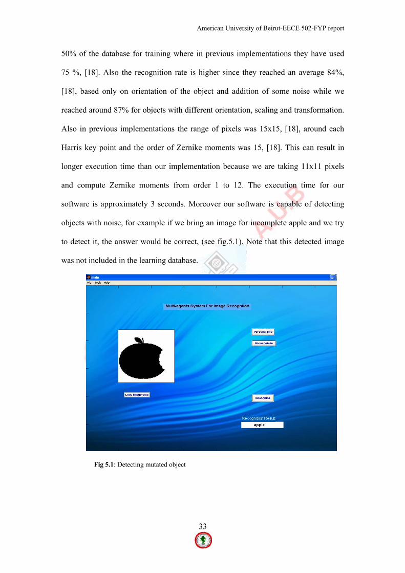
software is approximately 3 seconds. Moreover our software is capable of detecting
objects with noise, for example if we bring an image for incomplete apple and we try
to detect it, the answer would be correct, (see fig.5.1). Note that this detected image
was not included in the learning database.
Fig 5.1: Detecting mutated object

American University of Beirut-EECE 502-FYP report
34
Chapter 6
System Design Constraints Budget constraints:
Our FYP was done on a relatively small budget, since most of the work did
was coding. Thus we did not need any special hardware to buy. All that we needed
was our own laptops, some freely available software and MATLAB which is already
licensed by AUB. Further more the only cost that we incurred was to buy a switch for
20$ and a 2x10m CAT-5 cables to connect our laptops for about 20$. Thus the total
budget of our FYP is about 40$.
Device Cost
8-Port Switch 20$
Network Cables 20 $
Total 40 $
Environmental Aspect:
Our FYP is computer based, thus by itself it doesn’t cause any harm to the
environment directly. But one may take into account the energy needs of the project
in terms or processing power. This said the program does not require high processing
power; thus the system has an overall minimal Energy requirement.
Social Aspect:
Our FYP can really help people to recognize objects in images. Thus the use
of this technology is endless. It can be used in computer vision, medical imaging to
find certain abnormalities in medical images. Furthermore it can be used in military

American University of Beirut-EECE 502-FYP report
35
reconisense to recognize certain object from pictures taken from the satellite or
planes. Thus for example a high resolution photograph that is taken by a spy satellite
can be fed to our program, which in turn recognizes the objects that are shown in the
image. Missile launch pads, dams, airplanes, hangars, tanks, etc.
Ethical Aspect:
The code developed cannot be used in a malicious manner by itself, but if
modified it can be programmed to add certain commands over the network which can
render vulnerable computers unusable; on of these attacks could be SYN flooding or
any other packet, thus flooding the network with useless packets, thus we will have a
Denial of Service Attack. The use of switches decreases this, but this is still an issue
that should be tackled by the computer administrators and not our program. The ports
which we use to communicate over the network should be monitored for malicious
activity since infected computers can affect others on the network since they all are on
the same domain or workgroup; moreover they have write privileges on certain
directories on the main server (job manager). This FYP does not infringe on any
copyrights or the mental property of others unless stated in the references.
Health & Safety Aspects:
No harm can be done by this project, since it is a computer based program,
and thus no reason to cause harm to either humans or hardware. If properly used.
Manufacturability:
No manufacturing is required.

American University of Beirut-EECE 502-FYP report
36
Sustainability Aspects:
The program can definitely be improved and fine tweaked to achieve a better
recognition percentage. The trained database can be further enlarged to recognize
more objects. Thus in terms or sustainability it does not take a lot of effort or budget
to keep this process running.

American University of Beirut-EECE 502-FYP report
37
Conclusion
The need for better image understanding software is increasing since it can be
used in different fields such as medical, military, etc. According to the application of
this system, we are intending to apply complicated images for the detection process,
taking into account building the knowledge database that includes groups of images
for each class of objects. So, we are going to detect objects embedded in given images
regardless of the scale, translation, or rotation of the specified object. As a result, we
are going to implement this system for indoor 2-D processes; this may have benefits
regarding several applications such as robotics and security.

American University of Beirut-EECE 502-FYP report
38
List of references: [1] M. Hiramoto, T. Ogawa, and M. Haseyama, “A Novel Image Recognition Method
based on Feature-Extraction Vector Scheme”, 2004 International Conference on Image Processing (ICIP), pp. 3049-3052, Vol. 5, 2004.
[2] Dr. M.E.D Horani, Dr. F. Sukker, Eng. A. H. Horo, “Design and Implementation
of Artificial Intelligence system for 2-Dimensional Image Recognition”, pp. 465-466, IEEE, 2004
[3] Qing Chenl, Emil Petriul, Xiaoli Yang, “A Comparative Study of Fourier
Descriptors and Hu's Seven Moment Invariants for Image Recognition”, CCECE 2004, pp. 0103-0106, 2004.
[4] Dong-Gyu Sim, Hue-Kwang Kim and Due-I1 Oh, “Translation, Scale, and
Rotation Invariant Texture Descriptor for Texture-based Image Retrieval”, pp. 742-745, IEEE, 2000
[5] P. Pejnovic, Lj. Buturovic, Z. Stojiljkovic, “Object Recognition by Invariants”,
pp. 434-437, IEEE, 1992 [6] S Nishio H Takano T Maejima T Nakamura, “A study of image recognition
system”, pp. 112-116, NTT Data Communications Systems Corporation [7] A Khashman and KMCurtis, “Automatic Edge Detection Scheme”, pp. 535-538,
DSP 97, 1977 [8] Farahnaz Mohanna, Farzin Mokhtarian, “IMPROVED CURVATURE
ESTIMATION FOR ACCURATE LOCALISATION OF ACTIVE CONTOURS”, pp. 781-784, IEEE, 2001
[9] Tianyun Ma, Hemant D. Tagare, “Consistency and Stability of Active Contours with Euclidean and Non-Euclidean Arc Lengths”, pp. 1549-1559, IEEE TRANSACTIONS ON IMAGE PROCESSING, VOL. 8, NO. 11, NOVEMBER 1999 [10] Guillermo Sapiro, “Vector-Valued Active Contours”, pp. 680-685, IEEE,
1996 [11] Choksuriwong, Anant, Christophe Rosenberger, and Waleed W. Smari.
"Multi-agents System for Image Understanding." pp. 01-06. [12] "XITE."(2002) University of OSLO Retrieved Dec. 25, 2005 from
http://www.ifi.uio.no/forskning/grupper/dsb/Software/Xite/ftp/ [13] Mpich2. Retrieved Dec. 25, 2005, from http://www-
unix.mcs.anl.gov/mpi/mpich2/. [14] Habra, Abdul. "Neural Networks." *Neural Networks - An Introduction*.
2005.10.05. 22 May 2006 < http://www.tek271.com/articles/neuralNet/IntoToNeuralNets.html>.

American University of Beirut-EECE 502-FYP report
39
[15] Wikipedia contributors, 'Supervised learning', *Wikipedia, The Free
Encyclopedia,* 7 May 2006, 13:07 UTC, < http://en.wikipedia.org/w/index.php?title=Supervised_learning&oldid=51975666> [accessed 22 May 2006]
[16] Wikipedia contributors, 'Backpropagation', *Wikipedia, The Free
Encyclopedia,* 3 May 2006, 04:41 UTC, < http://en.wikipedia.org/w/index.php?title=Backpropagation&oldid=51316816> [accessed 22 May 2006]
[17] Abdallah, Samer. "Object Recognition via Invariance." *PhD. Thesis, *2000 [18] A.Choksuriwong, H.Laurent, C. Rosenberger, and C.Maaoui. “Object
Recognition using Local characterization and Zernike moments”. Laboratoire Vision et Bobotique-UPRES EA 2078 ENSI se Bourges- Université d’Orléans 10 boulevard Lahitolle. 18020 Bourger Cedex, France.
Related Documents