Final Term Paper Business Decision Method FORECASTING ...

1

Final Term Paper Business Decision Method

FORECASTING DEMAND OF MALAYSIAN

AUTOMOTIVE INDUSTRY & TRANSPORTATION PROBLEM ANALYSIS:

THE CASE OF PROTON

Instructor: Professor Jeh-Nan Pan

Group members:

Mohamad Rizal Abdul Hamid RA8967130

Iman Harymawan RA6967558

Hsu-Yuan Sun (Rebecca) RA7974011

NATIONAL CHENG KUNG UNIVERSITY INSTITUTE MASTER OF BUSINESS ADMINISTRATION

(IMBA) Fall Semester 2008

2

Content Abstract………………………………………………………………………... 3

Introduction…………………………………………………………………… 4

Literature Review………………………………………………………......... 6

Research Objectives………………………………………………………... 8

Research Hypotheses………………………………………………………. 8

Methodology…………………………………………………………………. 9

Result and Discussion……………………………………………………….. 12

Conclusion……………………………………………………………………. 20

References……………………………………………………………………. 21

Table 1: Fuel prices, inflation rate, and GDP per capita in Malaysia from 2000 to 2007……………………………………...

10

Table 2: Multiple regression analysis for fuel price, inflation rate and GDP per capita 2000-2007…………………………………

12

Table 3: Single regression for GDP per capita and Proton sales revenue 2000-2007………………………………………………..

13

Table 4: Vogel’s Approximation Method Result……………………….. 14

Figure 1: Study Framework…………………………………………………. 8

Figure 2: Malaysian fuel prices and inflation rate (2000-2007)……… 11

Figure 3: Malaysian GDP per capita (2000-2007)……………………… 11

3

Abstract

Malaysia is the tactics centre of automobile industry in the area of Southeast

Asia. Its national automobile manufacturer “Proton” plays an important role on

automobile industry development in the past ten years. This paper

investigates the correlation between the hike in fuel prices, inflation rate, and

GDP per capita with Proton’s sales revenue. Being the pillar of Malaysian

automotive industry, with the support by the government both in financial and

market wise, Proton seems to be formidable. Nevertheless, Proton has

recently reported to be suffering from shrinking sales. This recent decline has

been attributed to a number of factors, including mainly the rise in fuel prices.

For the purpose of forecasting Proton sales in successive year, casual

method, or the multiple Regression method is chosen in this study on

forecasting the sales revenue for the successive year. Key words: Malaysian automotive industry, Proton, fuel prices, GDP-per

capita, and Malaysian.

4

INTRODUCTION Industry Background The history of Malaysian automotive industry can be stretched back since the 1960’s. However, the manufacturing of Malaysian automotive industry was only visualized in the 1980’s. It was a giant leap for the Malaysian automobile industry (considering to the amount of investment involves) to manufacture the first Malaysian car, the Saga. The project was called the Malaysian National Car project and the company entrusted to undertake this project, Proton, was incorporated on 7 May 1983, under the name ‘Perusahaan Otomobil Nasional Berhad’. Established in 1983, Proton was the brain-child of Malaysia former Prime Minister. It is an ambition to turn Malaysia into Southeast Asia's new auto-making powerhouse. A shift intended by the government vying to be a high-tech player. Proton began its first operation in September 1985 at its first manufacturing plant in Shah Alam, Selangor. Initially the components of the car were entirely manufactured by Mitsubishi but slowly local parts were being used as technologies were transferred and skills were gained. As the pillar for Malaysian automotive industry, with the backing-up by the government in financially and market wise, Proton seems to be formidable. Sales rose tremendously, and by 2002 Proton held over 60 percent of the domestic market share. To date, there were at least 16 other manufacturing and assemblers companies operating in Malaysia—and almost identically competing for the same market. Despite being dominant, Proton is dubbed to be lacking in quality. Cheap materials, poor handling are among listed contributing to these factor. Proton exports cars to many other countries, and 14,706 Proton cars were exported in 2006, for instance, United Kingdom, South Africa, and Australia and in several other countries including the Middle East. Besides that, Proton cars has also been exporting a small volume of cars to Brunei, Indonesia, Nepal, Sri Lanka, Pakistan, Bangladesh, Taiwan , Cyprus and Mauritius. Capacity-wise, Proton is believed to be the largest and most modern automobile manufacturer in Southeast Asia, covering 862,000m2 employing 4,400 people (of which 2,400 are direct workers) with a production capacity of 150,000 units per year (two shift operation) at a production rate of 36 units per hour (Simpson, Sykes & Abdullah, 1998). Nevertheless, Proton has recently reported suffering from shrinking sales over the years (New Strait Times, 2006). This recent decline has been

5

attributed to a number of factors, including mainly the rise in fuel prices, tighter credit policies leading to less loans being approved as well as the fall in used car values which have affected trade-ins (Proton Annual Report, 2006). For the purpose of this study, I addition to the domestic fuel prices, we included the nation GDP per-capita (PPP) and also the inflation rate in predicting the sales revenue of Proton vehicles. Noteworthy, the full implementation of AFTA (ASEAN Free Trade Area) would subsequently push forward for more market liberalization. Currently, Malaysian market imposed a high tariff for vehicles crossing its boarders or CBU (complete built unit). Nonetheless, many manufactures and assembler opt for CKD (complete knocked-down) on making easy access to the Malaysian market. Reduction on taxes for imported cars combined with increase on consumer buying power might pose a threat for Proton prominence.

6

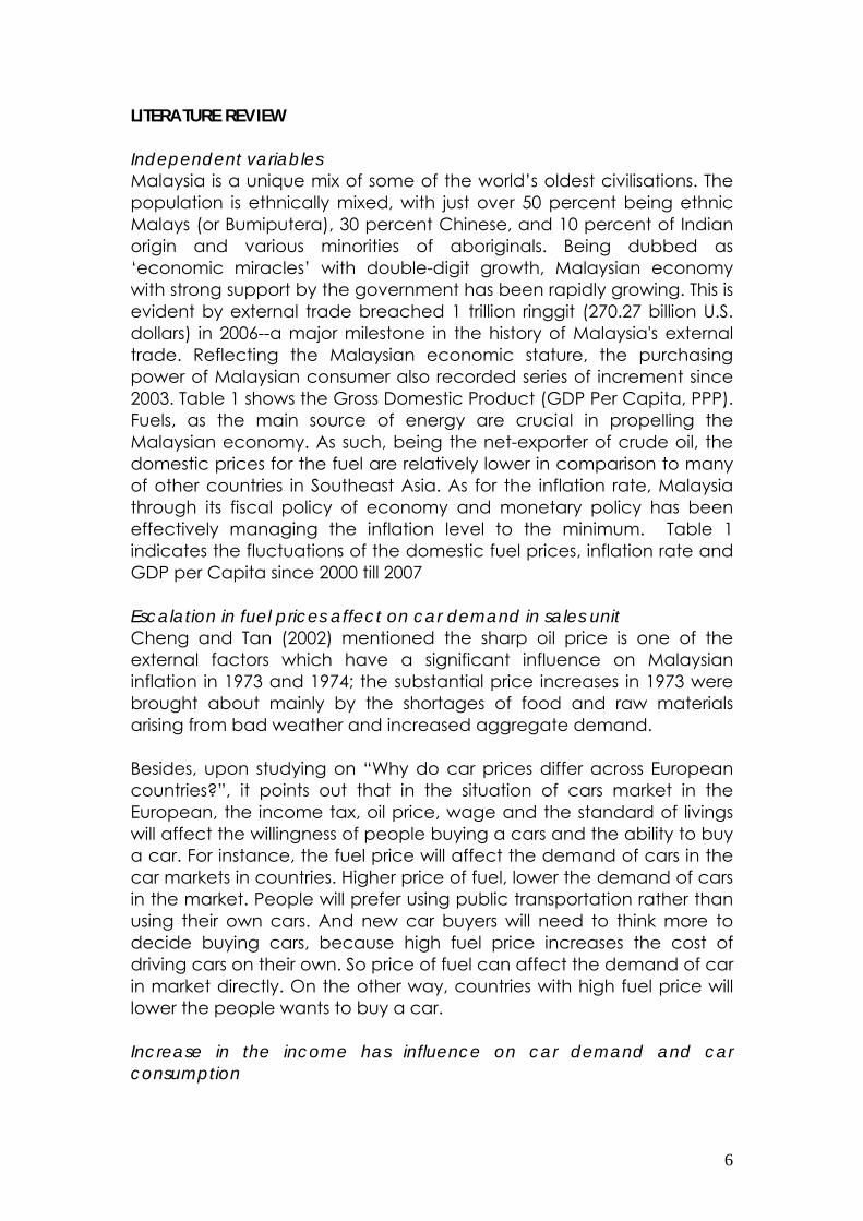
LITERATURE REVIEW Independent variables Malaysia is a unique mix of some of the world’s oldest civilisations. The population is ethnically mixed, with just over 50 percent being ethnic Malays (or Bumiputera), 30 percent Chinese, and 10 percent of Indian origin and various minorities of aboriginals. Being dubbed as ‘economic miracles’ with double-digit growth, Malaysian economy with strong support by the government has been rapidly growing. This is evident by external trade breached 1 trillion ringgit (270.27 billion U.S. dollars) in 2006--a major milestone in the history of Malaysia's external trade. Reflecting the Malaysian economic stature, the purchasing power of Malaysian consumer also recorded series of increment since 2003. Table 1 shows the Gross Domestic Product (GDP Per Capita, PPP). Fuels, as the main source of energy are crucial in propelling the Malaysian economy. As such, being the net-exporter of crude oil, the domestic prices for the fuel are relatively lower in comparison to many of other countries in Southeast Asia. As for the inflation rate, Malaysia through its fiscal policy of economy and monetary policy has been effectively managing the inflation level to the minimum. Table 1 indicates the fluctuations of the domestic fuel prices, inflation rate and GDP per Capita since 2000 till 2007 Escalation in fuel prices affect on car demand in sales unit Cheng and Tan (2002) mentioned the sharp oil price is one of the external factors which have a significant influence on Malaysian inflation in 1973 and 1974; the substantial price increases in 1973 were brought about mainly by the shortages of food and raw materials arising from bad weather and increased aggregate demand. Besides, upon studying on “Why do car prices differ across European countries?”, it points out that in the situation of cars market in the European, the income tax, oil price, wage and the standard of livings will affect the willingness of people buying a cars and the ability to buy a car. For instance, the fuel price will affect the demand of cars in the car markets in countries. Higher price of fuel, lower the demand of cars in the market. People will prefer using public transportation rather than using their own cars. And new car buyers will need to think more to decide buying cars, because high fuel price increases the cost of driving cars on their own. So price of fuel can affect the demand of car in market directly. On the other way, countries with high fuel price will lower the people wants to buy a car. Increase in the income has influence on car demand and car consumption

7

J. M. Dargay (2001) studies the effect of income on car ownership, and the results indicate that rising income leads to higher car ownership. Rising income makes it easier for households to own cars. Again J. Dargay (2007) continues to examine the effect of prices and income on car travel in the UK. It analyses the factors determining household car travel, and specifically the effects of household income and the prices of cars and motor fuels. The data shows the diffusion process: motoring has become more prevalent in successive generations. Car travel is more affected by car purchase costs than by fuel prices, implying that once obtained, cars are used despite rising variable costs for their use. On the other hand, car ownership is more sensitive to car purchase costs than to fuel prices as expected. Thus, car use responds more rapidly to changes in income and prices than car ownership. In a study on car demand in European countries also shows that the incomes of people will the main factor that affects the demand of cars in the market. The main income of people is wages, so high wages people with higher purchasing powers; they have higher demand for luxury goods, like cars, sport cars and houses. Graham and Glaister (2002) in survey about the response of motorists to fuel price changes and an assessment of the orders of magnitude of the relevant income and price effects. It means that the effect of price on fuel consumption and on motorists’ demand for road travel, and the demand for owning cars in heavily dependent on income. Also Eltony (1993) uses household data to quantify the behavioral responses that give rise to negative price elasticities of demand for gasoline. The result recognizes three main behavioral responses of households in Canada to changes in gasoline prices: drive fewer miles, purchase fewer cars and buy more efficient vehicles. Wetzel and Hoffer (1982) mentioned factors such as gasoline prices, styling changes, and demographic changes influenced the price elasticity of demand in each submarket differently using the disaggregated model. The models suggest that motor fuel price increases have a significant but temporary impact on consumer demand for the largest American car. Furthermore, as higher income individuals took delivery of previously ordered cars early in the model year. For this study, we found a close relation between these three main variables of the fuel prices, GDP per capita (PPP) and the inflation rate. As shown from Table 1, the relative increase in the GDP per capita is consistently followed with the increment in both the fuel and inflation rate. Chiefly, we believe these three variables are imperative in influencing the Proton sales revenue.

8

RESEARCH OBJECTIVES There are two main objectives of this study (1) the first objective is to develop and measure the strength of correlation between Proton sales with both the previous stated three variables of fuel price, the GDP per capita, and inflation rate. Noteworthy, as a national car manufacturer, consumers mainly choose Proton because of its cheaper prices in comparison with other imported vehicles. For that, we extended the analysis by separately measures the correlation using solely the GDP-per capita and the sales revenue. This, would provide us insight on how the Malaysian consumers behaviour or their selection on Proton product in relation with increase in the income. As for our second objective, this study seeks to answer the transportation problem in Proton distribution channel. As for now, Proton has three main facilities, separately located at Shah Alam, Tanjung Malim, and Cikarang with 10 different distributions channel throughout the nationwide located in Johor Bahru, Kedah, Kelantan, Kuala Lumpur, Pahang, Perak, Pulau Pinang, Sabah, Sarawak and Selangor. Using Vogel’s approximation method, we provide Proton with the optimal solution by taking into account the cost associated with each route alternatives.

RESEARCH HYPOTHESES In line with the objectives of the study, the null hypotheses were verified: Hypothesis 1: There is strong correlation between escalations in fuel prices, increment in GDP per capita, and inflation rate with Proton sales revenue. Hypothesis 2: Increase in GDP per-capita has strong effect on Proton sales revenue. THEORETICAL FRAMEWORK

Figure1: Study Framework

Proton sales revenue

Escalation in fuel prices

Increase in income

(GDP per capita)

Changes in

Inflation Rate

9

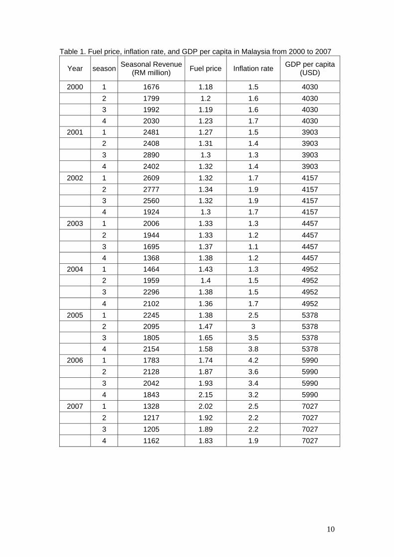
METHODOLOGY As for our first objective, the methodology chosen for this study is Multiple Regression. It is a causal method in which one variable, called a dependent variable, is related to one or more independent variables. The case study of Proton is seen to be corresponding with the method employed, bearing four elements for computation, the fuel prices (petrol price—in Ringgit Malaysia), The GDP per capita (PPP), inflation rate and sales revenue. Sales revenue is dependent variable which the manager wants to forecast, and petrol price, GDP per capita, and inflation rate are independent variables, assumed to affect the dependent variable. For our second objective, relating with the transportation distribution problem, we used Vogel’s approximation method. Vogel’s approximation method tackles the problem of finding an optimal initial solution by taking into account the cost associated with each route alternative. This is something contrary to that of northwest corner rule does include any regret or opportunity cost for its computation; thus, Vogel can be described as providing more accuracy in comparison to northwest corner. Collection of secondary data was obtained via numerous resources over the WWW and the company’s annual report, company newsletters, and local literature. It is also worth noting, the data collected concerning the annual unit of sales were varied from one resource to another. Nonetheless, for the sake of the study, the annual report published by Proton mainly will be used for its credibility. Microsoft Excel and QM software are used for the multiple regression computation and the transport method. Data Collected The data were quarterly recorded from 2000 to 2007 as table 1. Originally we wanted to collect 15 year records to analyze annually, but the sales revenue of Proton from 1993 to 1999 can not be acquired. GDP per capita is the annual record, so we offer the same value to each quarter of the year. There are totally 32 observations. The trend graphs of fuel prices, inflation rate and GDP per capita are as figure 2 and 3 respectively.

10

Table 1. Fuel price, inflation rate, and GDP per capita in Malaysia from 2000 to 2007

Year season Seasonal Revenue(RM million) Fuel price Inflation rate GDP per capita

(USD)

2000 1 1676 1.18 1.5 4030 2 1799 1.2 1.6 4030 3 1992 1.19 1.6 4030 4 2030 1.23 1.7 4030

2001 1 2481 1.27 1.5 3903 2 2408 1.31 1.4 3903 3 2890 1.3 1.3 3903 4 2402 1.32 1.4 3903

2002 1 2609 1.32 1.7 4157 2 2777 1.34 1.9 4157 3 2560 1.32 1.9 4157 4 1924 1.3 1.7 4157

2003 1 2006 1.33 1.3 4457 2 1944 1.33 1.2 4457 3 1695 1.37 1.1 4457 4 1368 1.38 1.2 4457

2004 1 1464 1.43 1.3 4952 2 1959 1.4 1.5 4952 3 2296 1.38 1.5 4952 4 2102 1.36 1.7 4952

2005 1 2245 1.38 2.5 5378 2 2095 1.47 3 5378 3 1805 1.65 3.5 5378 4 2154 1.58 3.8 5378

2006 1 1783 1.74 4.2 5990 2 2128 1.87 3.6 5990 3 2042 1.93 3.4 5990 4 1843 2.15 3.2 5990

2007 1 1328 2.02 2.5 7027 2 1217 1.92 2.2 7027 3 1205 1.89 2.2 7027 4 1162 1.83 1.9 7027

11

0

0.5

1

1.5

2

2.5

3

3.5

4

4.5

1 3 5 7 9 11 13 15 17 19 21 23 25 27 29 31

Fuel priceInflation rate

Fig. 2: Malaysian fuel prices and inflation rate (2000-2007)

0

1000

2000

3000

4000

5000

6000

7000

8000

2000 2001 2002 2003 2004 2005 2006 2007

GDP per capita

Fig. 3: Malaysian GDP per capita (2000-2007)

12

RESULTS AND DISCUSSION 1. The fuel price, inflation rate and GDP per capita with Proton sales

revenue (Multiple Regression Analysis) The result of the multiple regression analysis is as table 2. The r² value (0.54) for the model represents a middle strength of correlation, and the significance F value (6.4E-05) show there is a linear relationship. This value of r² implies 54 percent of variation in sales revenue is explained by these three variables of fuel price, GDP per capita and also inflation rate. There are three independent variables in the model. Three significance tests are performed to determine if fuel price, inflation rate and GDP per capita are significant. Using a 5% level of significance, the p-value of the fuel price is 0.54 greater than 0.05, so we cannot prove that the fuel prices have effect on sales revenue. From the literature review, the domestic fuel prices in Malaysia are relatively lower in comparison to many of other countries in Southeast Asia. And the price fluctuation has not been so large during the period from 2000 to 2007. In USA, the fuel price has only temporary effect on car purchasing. In European countries, people take public transportation instead of driving cars when the fuel prices are high. Therefore, it is possible the fuel prices in Malaysia have little effect on Proton sales revenue. Table 2. Multiple regression for fuel price, Inflation rate, and GDP per capita 2000-2007

Regression Statistics Multiple R 0.7341779R Square 0.5390172Adjusted R Square 0.4896262Standard Error 321.60817Observations 32

ANOVA

df SS MS F Significance F Regression 3 3386335.968 1128778.656 10.9132638 6.4E-05

Residual 28 2896090.751 103431.8125

Total 31 6282426.719

Coefficients Std. Error t Stat P-value Lower 95%

Upper 95%

Lower 95.0%

Upper 95.0%

Intercept 3342.5169 333.7792843 10.01415327 9.32887E-11 2658.801 4026.233 2658.801 4026.2328Fuel Price 337.48592 549.3538172 0.614332534 0.543955589 -787.8143 1462.786 -787.8143 1462.7862Inflation rate 200.48809 88.73806975 2.259324408 0.031837117 18.716394 382.2598 18.716394 382.25978GDP per capita -0.456826 0.133430989 -3.423687101 0.001921361 -0.730146 -0.1835 -0.730147 -0.183505

Nevertheless, the p-values of inflation rate and GDP per capita are both less than 0.05. Both of them have significant effect on Proton sales revenue. When the inflation rate is high, the sales revenue is also high. The high inflation rate generally comes from higher customer price

13

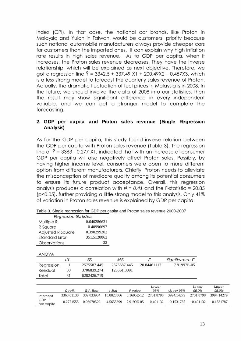
index (CPI). In that case, the national car brands, like Proton in Malaysia and Yulon in Taiwan, would be customers’ priority because such national automobile manufacturers always provide cheaper cars for customers than the imported ones. It can explain why high inflation rate results in high sales revenue. As to GDP per capita, when it increases, the Proton sales revenue decreases. They have the inverse relationship, which will be explained as next objective. Therefore, we got a regression line Ŷ = 3342.5 + 337.49 X1 + 200.49X2 – 0.457X3, which is a less strong model to forecast the quarterly sales revenue of Proton. Actually, the dramatic fluctuation of fuel prices in Malaysia is in 2008. In the future, we should involve the data of 2008 into our statistics, then the result may show significant difference in every independent variable, and we can get a stronger model to complete the forecasting. 2. GDP per capita and Proton sales revenue (Single Regression

Analysis) As for the GDP per capita, this study found inverse relation between the GDP per-capita with Proton sales revenue (Table 3). The regression line of Ŷ = 3363 - 0.277 X1, indicated that with an increase of consumer GDP per capita will also negatively affect Proton sales. Possibly, by having higher income level, consumers were open to more different option from different manufacturers. Chiefly, Proton needs to alleviate the misconception of mediocre quality among its potential consumers to ensure its future product acceptance. Overall, this regression analysis produces a correlation with r² = 0.41 and the F-statistic = 20.85 (p<0.05), further providing a little strong model to this analysis. Only 41% of variation in Proton sales revenue is explained by GDP per capita. Table 3. Single regression for GDP per capita and Proton sales revenue 2000-2007

Regression Statistics Multiple R 0.640286631R Square 0.40996697Adjusted R Square 0.390299202Standard Error 351.5128862Observations 32

ANOVA

df SS MS F Significance F Regression 1 2575587.445 2575587.445 20.84461117 7.91997E-05

Residual 30 3706839.274 123561.3091

Total 31 6282426.719

Coeff. Std. Error t Stat P-value Lower 95% Upper 95%

Lower 95.0%

Upper 95.0%

Intercept 3363.01130 309.033934 10.8823366 6.1605E-12 2731.8798 3994.14279 2731.8798 3994.14279GDP per capita -0.2771555 0.06070529 -4.5655899 7.9199E-05 -0.401132 -0.1531787 -0.401132 -0.1531787

14

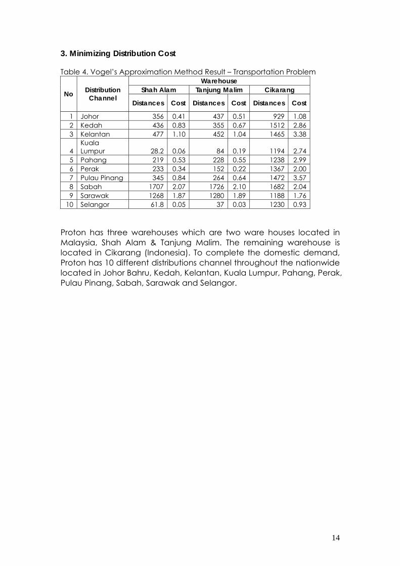
3. Minimizing Distribution Cost Table 4. Vogel’s Approximation Method Result – Transportation Problem

Warehouse Shah Alam Tanjung Malim Cikarang No Distribution

Channel Distances Cost Distances Cost Distances Cost

1 Johor 356 0.41 437 0.51 929 1.08 2 Kedah 436 0.83 355 0.67 1512 2.86 3 Kelantan 477 1.10 452 1.04 1465 3.38

4 Kuala Lumpur 28.2 0.06 84 0.19 1194 2.74

5 Pahang 219 0.53 228 0.55 1238 2.99 6 Perak 233 0.34 152 0.22 1367 2.00 7 Pulau Pinang 345 0.84 264 0.64 1472 3.57 8 Sabah 1707 2.07 1726 2.10 1682 2.04 9 Sarawak 1268 1.87 1280 1.89 1188 1.76

10 Selangor 61.8 0.05 37 0.03 1230 0.93 Proton has three warehouses which are two ware houses located in Malaysia, Shah Alam & Tanjung Malim. The remaining warehouse is located in Cikarang (Indonesia). To complete the domestic demand, Proton has 10 different distributions channel throughout the nationwide located in Johor Bahru, Kedah, Kelantan, Kuala Lumpur, Pahang, Perak, Pulau Pinang, Sabah, Sarawak and Selangor.

15

Initial solution We used VAM in calculating Proton Distribution cost for the ten states Iterations 1 To From

Johor Bahru Kedah Kelantan Kuala

Lumpur Pahang Perak Pulau Pinang Sabah Sarawak Selangor Dummy Supply

Shah Alam

0.41 15103

0.83 x

1.10 x

0.06 7639

0.53 x

0.34 x

0.84 x

2.07 x

1.87 x

0.05 x

0 177258

200000

Tanjung Malim

0.51 x

0.67 9254

1.04 7589

0.19 x

0.55 7247

0.22 11952

0.64 7214

2.10 14418

1.89 (-) 11847

0.03 23237

0 (+) 57242

150000

Cikarang 1.08 x

2.86 x

3.38 x

2.74 x

2.99 x

2.00 x

3.57

x

2.04 x

1.76 x (+)

0.93 x

0 40000 (-)

40000

Demand 15103 9254 7589 7639 7247 11952 7214 14418 11847 23237 274500 390000

Stepping-Stone Method: Least-cost solution

Closed path for ICikarang – Kelantan = 2.34

Closed path for ICikarang – Kuala Lumpur =

2.68

Closed path for ICikarang – Pahang = 2.44

Closed path for ICikarang – Perak = 1.78

Closed path for ICikarang – Pulau Pinang =

2.93

Closed path for ICikarang – Sabah = -0.06

Closed path for IShah Alam – Kedah

= +SAKe – SADummy + TMDummy – TMKe

= +0.83 – 0 + 0 – 0.67 = 0.16

Closed path for IShah Alam – Kelantan = 0.06

Closed path for IShah Alam – Pahang = -0.02

Closed path for IShah Alam – Perak = 0.12

Closed path for IShah Alam – Pulau Pinang =

0.2

Closed path for IShah Alam – Sabah = -0.03

Closed path for IShah Alam – Sarawak = -0.02

Closed path for IShah Alam – Selangor = 0.02

Closed path for ITanjung Malim – Johor = 0.1

Closed path for ITanjung Malim – Kuala Lumpur = 0.13

Closed path for ICikarang – Johor = 0.67

Closed path for ICikarang – Kedah = 2.19

16

Iteration 2 To From



Shah Alam

0.41 15103

0.83 x

1.10 x

0.06 7639

0.53 x

0.34 x

0.84 x

2.07 x

1.87 x

0.05 x

0 177258

200000

Tanjung Malim

0.51 x

0.67 9254

1.04 7589

0.19 x

0.55 7247

0.22 11952

0.64 7214

2.10 (-) 14418

1.89 x

0.03 23237

0 (+) 69089

150000

Cikarang 1.08 x

2.86 x

3.38 x

2.74 x

2.99 x

2.00 x

3.57

x

2.04 x (+)

1.76 11847

0.93 x

0 28153 (-)

40000

Demand 15103 9254 7589 7639 7247 11952 7214 14418 11847 23237 274500 390000






2.68




2.93

f i

Closed path for IShah Alam – Kedah


= +0.83 – 0 + 0 – 0.67 = 0.16




Closed path for IShah Alam – Pulau Pinang = 0.2

Closed path for IShah Alam – Sabah = -0.03

Closed path for IShah Alam – Sarawak = 0.11




Closed path for ITanjung Malim – Sarawak = 0.13

17

Iteration 3 To From



Shah Alam

0.41 15103

0.83 x

1.10 x

0.06 7639

0.53 (+) x

0.34 x

0.84 x

2.07 x

1.87 x

0.05 x

0 (-) 177258

200000

Tanjung Malim

0.51 x

0.67 9254

1.04 7589

0.19 x

0.55 (-) 7247

0.22 11952

0.64 7214

2.10 x

1.89 x

0.03 23237

0 (+) 83507

150000

Cikarang 1.08 x

2.86 x

3.38 x

2.74 x

2.99 x

2.00 x

3.57

x

2.04 14418

1.76 11847

0.93 x

0 13735

40000

Demand 15103 9254 7589 7639 7247 11952 7214 14418 11847 23237 274500 390000






2.68




Closed path for IShah Alam - Kedah


= +0.83 – 0 + 0 – 0.67 = 0.16




Closed path for IShah Alam – Pulau Pinang =

0.2

Closed path for IShah Alam – Sabah = 0.03




Closed path for ITanjung Malim – Kuala Lumpur =

0.13

Closed path for ITanjung Malim – Sabah = 0.06


18

Iteration 4 To From



Shah Alam

0.41 15103

0.83 x

1.10 x

0.06 7639

0.53 7247

0.34 x

0.84 x

2.07 x

1.87 x

0.05 x

0 170011

200000

Tanjung Malim

0.51 x

0.67 9254

1.04 7589

0.19 x

0.55 x

0.22 11952

0.64 7214

2.10 x

1.89 x

0.03 23237

0 90754

150000

Cikarang 1.08 x

2.86 x

3.38 x

2.74 x

2.99 x

2.00 x

3.57

x

2.04 14418

1.76 11847

0.93 x

0 13735

40000

Demand 15103 9254 7589 7639 7247 11952 7214 14418 11847 23237 274500 390000






2.68




Closed path for IShah Alam - Kedah


= +0.83 – 0 + 0 – 0.67 = 0.16



Closed path for IShah Alam – Pulau Pinang = 0.2

Closed path for IShah Alam – Sabah = 0.03





Closed path for ITanjung Malim – Pahang = 0.02

Closed path for ITanjung Malim – Sabah = 0.06


19

Total Cost Shah Alam to Johor Bahru = 15013 units x RM0.41 = RM6155.33 Shah Alam to Kuala Lumpur = 7639 units x RM0.06 = RM458.34 Shah Alam to Pahang = 7247 units x RM0.53 = RM3841 Tanjung Malim to Kedah = 9254 units x RM0.67 = RM6200.18 Tanjung Malim to Kelantan = 7589 units x RM1.04 = RM7892.56 Tanjung Malim to Perak = 11952 units x RM0.22 = RM2629.44 Tanjung Malim to Pulau Pinang = 7214 units x RM0.64 = RM4616.96 Tanjung Malim to Selangor = 23237 units x RM0.03 = RM697.11 Cikarang to Sabah = 14418 units x RM2.04 = RM29412.72 Cikarang to Sarawak = 11847 units x RM1.76 = RM20850.72 6155.33 + 458.34 + 3841 + 6200.18 + 7892.56 + 2629.44 + 4616.96 + 697.11 + 29412.72 + 20850.72 = RM82754.36 @ NTD774, 878.73 Optimal Solution We used Vogel’s approximation method to find the initial solution of this transportation problem. We found four iterations in order to arrive at the optimal solution. To derive the least-cost solution we opt to use the stepping stone method. The stepping stone method is an iterative technique for moving from an initial feasible solution to an optimal feasible solution. This process has two distinct parts: The first involves testing the current solution to determine if improvement is possible, and the second part involves making changes to the current solution in order to obtain an improved solution. This process continues until the optimal solution is reached. For the stepping stone method to be applied to a transportation problem, one rule about the number of shipping routes being used must first be observed: The number of occupied routes must always be equal to one less than the sum of the number of rows plus the number of columns. In Proton transportation problem, this means that the initial solution must have 10 + 3 – 1 = 12 squares used. In 4 initial feasible solution of this problem, we found that only 10 squares routes occupied. It means that degeneracy problem arise in this problem. To handle degeneracy problems we create artificially occupied cell in one of the unused squares and then treat that square as if it were occupied. The square chosen must be in such a position as to allow all stepping stone paths to be closed, although there is usually a good deal of flexibility in selecting the unused square that will receive the zero. In the iteration 1, we found that the biggest negative improvement index of closed path is from Cikarang to Sarawak, which is equal to -

20

0.13. It means that we can increase the cost saving by making use of the (currently unused) Cikarang to Sarawak route. Then we move the allocation distribution for 11847 cars from Tanjung Malim warehouse to Cikarang warehouse to complete the demand from Sarawak. In the iteration 2, we found that the biggest negative improvement index of closed path is from Cikarang to Sabah, which is equal to -0.06. It means that we can increase the cost saving by making use of the (currently unused) Cikarang to Sabah route. Then we move the allocation distribution for 14418 cars from Tanjung Malim warehouse to Cikarang warehouse to complete the demand from Sabah. In the iteration 3, we found that the biggest negative improvement index of a closed path is from Shah Alam to Pahang, which is equal to -0.02. It means that we can increase the cost saving by making use of the (currently unused) Shah Alam to Pahang route. Then we move the allocation distribution for 7247 cars from Tanjung Malim warehouse to Shah Alam warehouse to complete the demand from Pahang. In the iteration 4, we found that all improvement index of closed path shown positive number. It has meaning that there is no opportunity to minimize the cost, because this initial feasible solution achieve the optimal solution. Conclusion

Proton sales have been declining for recent years. The competition from local

manufacturers as well as foreign importers is increasing. The customers have

stronger purchasing power and more options in the car market. How to

enhance the production quality and recover the market share is a significant

issue for Proton. In 2008, Proton starts to cooperate with Detroit Electrics to

develop the electric cars, and plans to manufacture 100,000 electric cars by

2010. One of the major strategies of Proton in recent years is to produce fuel-

efficient and energy-saving cars to coordinate with market demand and

environmental protection. To capture a larger market in China is also an

opportunity for Proton to increase the sales volume.

References https://www.cia.gov/redirects/ciaredirect.html http://www.indexmundi.com/malaysia/

21

http://www.maa.org.my/info_summary.htm http://www.statoids.com/umy.html http://www.business-in-asia.com/asia/asia_inflation.html http://financialindependent.blogspot.com/2008/03/fd-savings-inflation-and-

epf-rates-in.html http://www.carstandard.com/blog/68/malaysia-petrol-fuel-price-increase-

historical-record.html http://www.proton.com/about_proton/investor_relations/financial_reports.ph

p http://investintaiwan.nat.gov.tw/zh-tw/env/stats Cheng, M.-Y., & Tan, H.-B. (2002). Inflation in Malaysia. International Journal of

Social Economics, 29(5). Correlation and Linear Regression: Retrieved on 16 November 2007 on

http://richardbowles.tripod.com/maths/correlation/corr.htm Dargay, J. (2007). The effect of prices and income on car travel in the UK.

Transportation Research Part A, 41, 949–960. Dargay, J. M. (2001). The effect of income on car ownership: evidence of

asymmetry. Transportation Research Part A, 35, 807-821. Eileen Ng, Malaysian New Auto Sales Fell in 2006, International Business Times,

January 25, 2007: Retrieved on 15 November 2007 from http://www.ibtimes.com/subsection/globalnews/asiapacific.htm

Graham, D. J., & Glaister, S. (2002). The demand for automobile fuel: A survey

of elasticities. Journal of Transport Economics and Policy, 36(1), 1-26. Linear Regression and Excel, Clemson University, 2000: Retrieved on 16

November 2007 from http://phoenix.phys.clemson.edu/tutorials/excel/regression.html

Malaysia Customer Satisfaction Index (CSI), J.D. Power and Associates, Mc-

Graw Hill Companies: Retrived on 17 November 2007 from http://www.jdpower.com/corporate/awards/industry/default.aspx

Malaysia's Proton waives 16.5 million pound Lotus debt, BizNewsDataBank:

Retrieved on 16 November 2007 on http://www.english.biznewsdb.com/

22

Malaysia's Proton pins hopes on new car to lift sales, return to profit, International Herald Tribune, Retrieved on 16 November 2007 from http://www.iht.com/pages/business/index.php

Proton Annual Report 2002 until 2003, Perusahaan Otomobil Nasional Sdn.

Bhd.: Retrieved on 17 November 2007 from http://media.proton.com/public/dl_annualreport.php

Proton bomb, Economist, Academic Search Premier, Vol. 371, August 2004, Proton (carmaker), Wikipedia: The free encyclopaedia: Retrieved on 13

November 2007 from http://en.wikipedia.org/wiki/Proton_%28carmaker%29

Ritzman, L.P, Krajewski, L.J, 2003, Foundations of Operation management,

Prentice Hall, New Jersey. Render, B., Ralph M. Stair, J., & Hanna, M. E. (2006). Quantitative Analysis for

Management (9 ed.). Upper Saddle River, New Jersey: Pearson Education Inc.

Simpson, M., Sykes, G. and Abdullah, A., Case study: transitory JIT at Proton

Cars, Malaysia, Sheffield University Management School, Sheffield, UK, International Journal of

Physical Distribution & Logistics Management, Vol. 28 No. 2, 1998, pp. 121-142.

Tamar Gabilaai, Malaysian Proton and AFTA: threat or advantage? TED Case

Studies Number, June 2001: Retrived on 14 November 2007 from http://www.american.edu/TED/proton.htm#r1

Wetzel, J., & Hoffer, G. (1982). Consumer demand for automobiles: A

disaggregated market approach. Journal of consumer research, 9, 195-199.

Zuraimi Abdullah, Poor sales prompt EON to offer VSS, New Strait Times, July 26,

2006: Retrieved on 14 November 2007 from http://www.highbeam.com

Final Term Paper Business Decision Method FORECASTING ...

Documents