Final SGRE paper-Heba-m

Smart Grid and Renewable Energy, 2013, *, **-**

doi:10.4236/sgre.2013.***** Published Online *** 2013 (http://www.scirp.org/journal/sgre)

Copyright © 2013 SciRes. SGRE

Sizing of STATCOM to Enhance Voltage Stability of

Power Systems for Normal and Contingency Cases

Heba A. Hassan1,2*

, Zeinab H. Osman2, Abd El-Aziz Lasheen

3

1 Electrical and Computer Engineering Department, Dhofar University, Salalah, Oman; 2 Electrical Power and Machines Department,

Cairo University, Giza, Egypt; 3 Electricity Holding Company, Ministry of Electricity and Energy, Cairo, Egypt

Email: [email protected]

Accepted December 10th, 2013.

ABSTRACT

The electric power infrastructure that has served huge loads for so long is rapidly running up against many limitations.

Out of many challenges is to operate the power system in secure manner such that the operation constraints are fulfilled

under both normal and contingency conditions. Smart grid technology offers valuable techniques that can be deployed

within the very near future or which are already deployed nowadays. Flexible AC Transmission Systems (FACTS)

devices have been introduced to solve various power system problems. In literature, most of the methods proposed for

sizing the FACTS devices consider only the normal operating conditions of power systems. Consequently, some

transmission lines are heavily loaded in contingency case and the system voltage stability becomes a power

transfer-limiting factor. This paper presents a technique for determining the proper rating/size of FACTS devices,

namely the Static Synchronous Compensator (STATCOM), while considering contingency cases. The paper also veri-

fies that the weakest bus determined by eigenvalue and eigenvectors method is the best location for STATCOM. The

rating of STATCOM is specified according to the required reactive power needed to improve voltage stability under

normal and contingency cases. Two case system studies are investigated; a simple 5-bus system and the IEEE 14-bus

system. The obtained results verify that the rating of STATCOM can be determined according to the worst contingency

case, and through proper control it can still be effective for normal and other contingency cases.

Keywords: STATCOM; Voltage Stability; Contingency; Eigenvalues and Eigenvectors; Newton-Raphson Load Flow.

1. Introduction

In a competitive energy market, the grid mostly operates

very close to its maximum capacity. Therefore,

congestions may occur due to unexpected line outage,

generator outage, sudden increase of demand, failures of

equipments, etc. Hence, network congestion has become

a major concern for smart grids. However, in the context

of the smart grid, it is possible to obtain measurements

from throughout the grid to identify and implement the

necessary control actions in sub-second time frames.

Thus, voltage instability and collapse that may lead to

the blackout can be avoided, if suitable monitoring is

used and application of a preventive control is taken. In

this context, FACTS devices can be applied to improve

the voltage stability of power systems.

One of the most recent technologies that has always

grasped the attention of researchers in power engineering

is the Flexible AC Transmission Systems (FACTS). This

technique appeared in literature for the first time in 1989

when Narian Hingorani defined FACTS as „The concept

of using solid-state power electronic devices mainly

thyristor for power flow control at transmission level‟,

[1]. Recent advances in the area of voltage source

converters (VSC) have added also to this area of

research. In addition, there is an increasing interest in

using FACTS devices in the operation and control of

power systems. These devices are characterized by fast

response, high reliability and wide operating range,

[2-5].

Voltage stability is a problem in power systems which

are heavily loaded, faulted or have a shortage of reactive

power. The nature of voltage stability can be analyzed by

examining the production, transmission and consumption

of reactive power. The problem of voltage stability

concerns the whole power system, although it usually has

a large involvement in one critical area of the power

system. The voltage stability can be improved by

allocating FACTS devices, [6-13].

The contingency ranking methods for voltage stability

Copyright © 2011 SciRes. POS

analysis are based on sensitivities of voltage stability

margin, the curve fitting method, simultaneous

computation of multiple contingency cases and

parallel/distributed computation algorithms, [14-17]. The

state of power system voltage stability can be described

in terms of reactive power losses, [18]. When the power

system is stressed, reactive power losses increase

compared to the operation point. In this case, the reactive

power losses of outages need to be calculated and the

ranking of contingencies can be directly based on them.

The minimum singular value of the load-flow Jacobian

matrix is zero at the voltage collapse point, [19-20]. It is

used as an indicator to quantify proximity to post

disturbance maximum loading point. The use of the

indicator requires the computation of post-disturbance

load flows for each outage. The value of the minimum

singular value of the load flow Jacobian matrix is also

sensitive to limitations and changes of the reactive power

output. Computing the minimum singular values at the

stressed operation point can increase the accuracy of the

method.

This paper presents an algorithm to determine the rated

capacity of STATCOM to improve the static voltage

stability of a power system under normal and

contingency conditions. This is achieved through

rescheduling the reactive power control variables of

STATCOM. The algorithm utilizes the method of the

eigenvalues and eigenvectors of the load flow Jacobian

which is a proximity indicator that determines the

weakest bus in the system. The rating of STATCOM is

proposed to be determined while taking into account its

suitability for both normal and contingency cases.

Section 2 overviews the basic structure and operation

theory of STATCOM. In Section 3, the saddle-node

bifurcation and system voltage instability are explained.

Section 4 presents the algorithm of the developed

technique and MATLAB package for the optimal

allocation of STATCOM. Results of two case-studies are

presented in Section 5 for a 5-bus system model and

IEEE 14-bus power system. The given results included

system study and load flow analysis under normal

operating conditions and in case of contingencies with

and without STATCOM after the implementation of the

developed device allocation technique. The main

conclusions and contribution of the paper are mentioned

in Section 6.

2. STATCOM Device

STATCOM is a static synchronous generator operated as

a shunt connected static VAR compensator whose

capacitive or inductive output current can be controlled

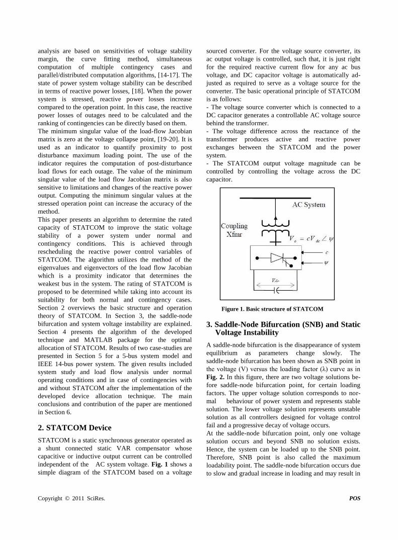
independent of the AC system voltage. Fig. 1 shows a

simple diagram of the STATCOM based on a voltage

sourced converter. For the voltage source converter, its

ac output voltage is controlled, such that, it is just right

for the required reactive current flow for any ac bus

voltage, and DC capacitor voltage is automatically ad-

justed as required to serve as a voltage source for the

converter. The basic operational principle of STATCOM

is as follows:

- The voltage source converter which is connected to a

DC capacitor generates a controllable AC voltage source

behind the transformer.

- The voltage difference across the reactance of the

transformer produces active and reactive power

exchanges between the STATCOM and the power

system.

- The STATCOM output voltage magnitude can be

controlled by controlling the voltage across the DC

capacitor.

Figure 1. Basic structure of STATCOM

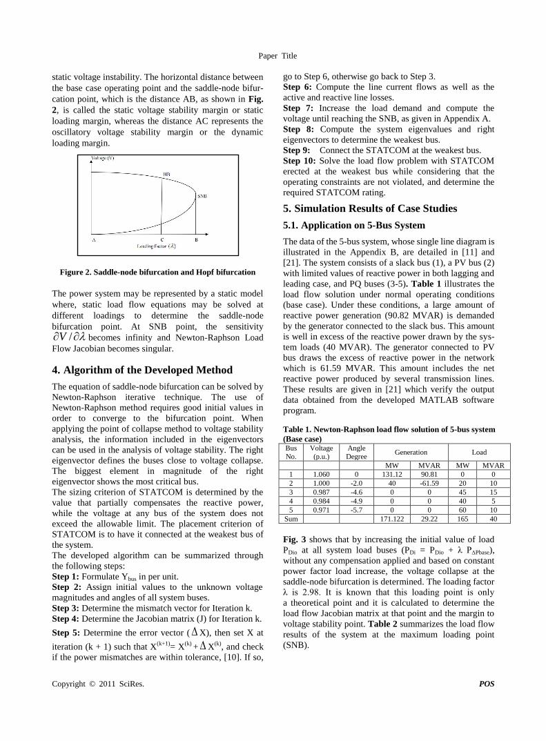
3. Saddle-Node Bifurcation (SNB) and Static Voltage Instability

A saddle-node bifurcation is the disappearance of system

equilibrium as parameters change slowly. The

saddle-node bifurcation has been shown as SNB point in

the voltage (V) versus the loading factor (λ) curve as in

Fig. 2. In this figure, there are two voltage solutions be-

fore saddle-node bifurcation point, for certain loading

factors. The upper voltage solution corresponds to nor-

mal behaviour of power system and represents stable

solution. The lower voltage solution represents unstable

solution as all controllers designed for voltage control

fail and a progressive decay of voltage occurs.

At the saddle-node bifurcation point, only one voltage

solution occurs and beyond SNB no solution exists.

Hence, the system can be loaded up to the SNB point.

Therefore, SNB point is also called the maximum

loadability point. The saddle-node bifurcation occurs due

to slow and gradual increase in loading and may result in

Paper Title


static voltage instability. The horizontal distance between

the base case operating point and the saddle-node bifur-

cation point, which is the distance AB, as shown in Fig.

2, is called the static voltage stability margin or static

loading margin, whereas the distance AC represents the

oscillatory voltage stability margin or the dynamic

loading margin.

Figure 2. Saddle-node bifurcation and Hopf bifurcation

The power system may be represented by a static model

where, static load flow equations may be solved at

different loadings to determine the saddle-node

bifurcation point. At SNB point, the sensitivity

/V becomes infinity and Newton-Raphson Load

Flow Jacobian becomes singular.

4. Algorithm of the Developed Method

The equation of saddle-node bifurcation can be solved by

Newton-Raphson iterative technique. The use of

Newton-Raphson method requires good initial values in

order to converge to the bifurcation point. When

applying the point of collapse method to voltage stability

analysis, the information included in the eigenvectors

can be used in the analysis of voltage stability. The right

eigenvector defines the buses close to voltage collapse.

The biggest element in magnitude of the right

eigenvector shows the most critical bus.

The sizing criterion of STATCOM is determined by the

value that partially compensates the reactive power,

while the voltage at any bus of the system does not

exceed the allowable limit. The placement criterion of

STATCOM is to have it connected at the weakest bus of

the system.

The developed algorithm can be summarized through

the following steps:

Step 1: Formulate Ybus in per unit.

Step 2: Assign initial values to the unknown voltage

magnitudes and angles of all system buses.

Step 3: Determine the mismatch vector for Iteration k.

Step 4: Determine the Jacobian matrix (J) for Iteration k.

Step 5: Determine the error vector (X), then set X at

iteration (k + 1) such that X(k+1)

= X(k)

+X(k)

, and check

if the power mismatches are within tolerance, [10]. If so,

go to Step 6, otherwise go back to Step 3.

Step 6: Compute the line current flows as well as the

active and reactive line losses.

Step 7: Increase the load demand and compute the

voltage until reaching the SNB, as given in Appendix A.

Step 8: Compute the system eigenvalues and right

eigenvectors to determine the weakest bus.

Step 9: Connect the STATCOM at the weakest bus.

Step 10: Solve the load flow problem with STATCOM

erected at the weakest bus while considering that the

operating constraints are not violated, and determine the

required STATCOM rating.

5. Simulation Results of Case Studies

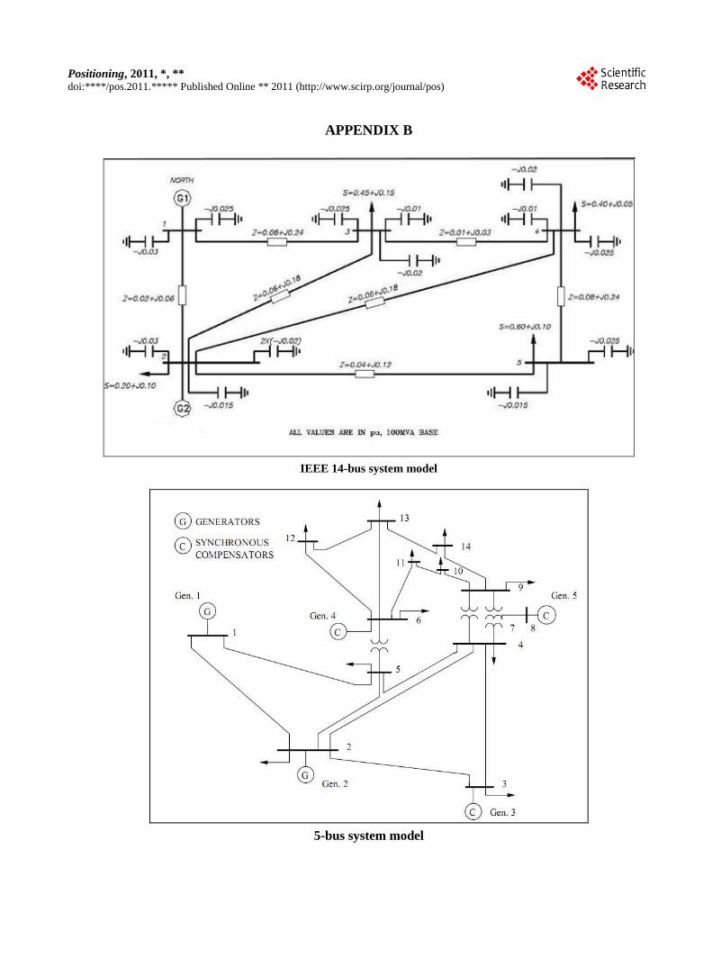
5.1. Application on 5-Bus System

The data of the 5-bus system, whose single line diagram is

illustrated in the Appendix B, are detailed in [11] and

[21]. The system consists of a slack bus (1), a PV bus (2)

with limited values of reactive power in both lagging and

leading case, and PQ buses (3-5). Table 1 illustrates the

load flow solution under normal operating conditions

(base case). Under these conditions, a large amount of

reactive power generation (90.82 MVAR) is demanded

by the generator connected to the slack bus. This amount

is well in excess of the reactive power drawn by the sys-

tem loads (40 MVAR). The generator connected to PV

bus draws the excess of reactive power in the network

which is 61.59 MVAR. This amount includes the net

reactive power produced by several transmission lines.

These results are given in [21] which verify the output

data obtained from the developed MATLAB software

program.

Table 1. Newton-Raphson load flow solution of 5-bus system

(Base case)

Load Generation Angle

Degree

Voltage

(p.u.)

Bus

No.

MVAR MW MVAR MW

0 0 90.81 131.12 0 1.060 1

10 20 -61.59 40 -2.0 1.000 2

15 45 0 0 -4.6 0.987 3

5 40 0 0 -4.9 0.984 4

10 60 0 0 -5.7 0.971 5

40 165 29.22 171.122 Sum

Fig. 3 shows that by increasing the initial value of load

PDio at all system load buses (PDi = PDio + λ P∆Pbase),

without any compensation applied and based on constant

power factor load increase, the voltage collapse at the

saddle-node bifurcation is determined. The loading factor

λ is 2.98. It is known that this loading point is only

a theoretical point and it is calculated to determine the

load flow Jacobian matrix at that point and the margin to

voltage stability point. Table 2 summarizes the load flow

results of the system at the maximum loading point

(SNB).


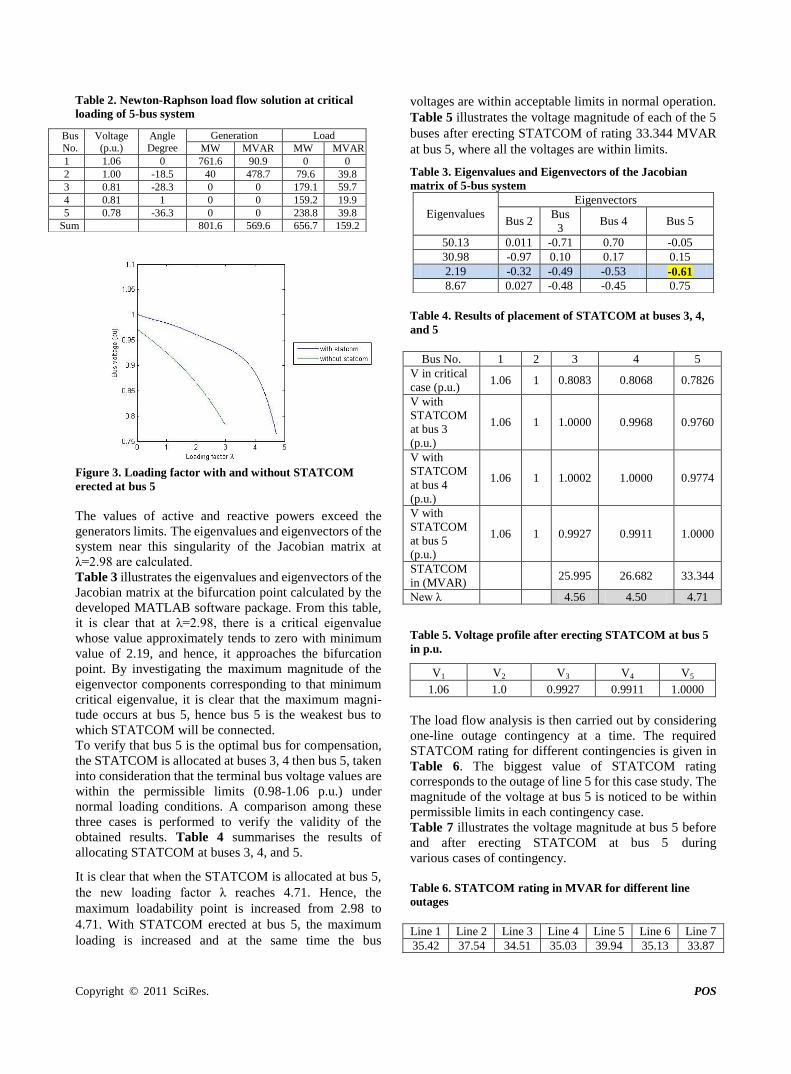
Table 2. Newton-Raphson load flow solution at critical

loading of 5-bus system

Figure 3. Loading factor with and without STATCOM

erected at bus 5

The values of active and reactive powers exceed the

generators limits. The eigenvalues and eigenvectors of the

system near this singularity of the Jacobian matrix at

λ=2.98 are calculated.

Table 3 illustrates the eigenvalues and eigenvectors of the

Jacobian matrix at the bifurcation point calculated by the

developed MATLAB software package. From this table,

it is clear that at λ=2.98, there is a critical eigenvalue

whose value approximately tends to zero with minimum

value of 2.19, and hence, it approaches the bifurcation

point. By investigating the maximum magnitude of the

eigenvector components corresponding to that minimum

critical eigenvalue, it is clear that the maximum magni-

tude occurs at bus 5, hence bus 5 is the weakest bus to

which STATCOM will be connected.

To verify that bus 5 is the optimal bus for compensation,

the STATCOM is allocated at buses 3, 4 then bus 5, taken

into consideration that the terminal bus voltage values are

within the permissible limits (0.98-1.06 p.u.) under

normal loading conditions. A comparison among these

three cases is performed to verify the validity of the

obtained results. Table 4 summarises the results of

allocating STATCOM at buses 3, 4, and 5.

It is clear that when the STATCOM is allocated at bus 5,

the new loading factor λ reaches 4.71. Hence, the

maximum loadability point is increased from 2.98 to

4.71. With STATCOM erected at bus 5, the maximum

loading is increased and at the same time the bus

voltages are within acceptable limits in normal operation.

Table 5 illustrates the voltage magnitude of each of the 5

buses after erecting STATCOM of rating 33.344 MVAR

at bus 5, where all the voltages are within limits.

Table 3. Eigenvalues and Eigenvectors of the Jacobian

matrix of 5-bus system

Table 4. Results of placement of STATCOM at buses 3, 4,

and 5

5 4 3 2 1 Bus No.

0.7826 0.8068 0.8083 1 1.06 V in critical

case (p.u.)

0.9760 0.9968 1.0000 1 1.06

V with

STATCOM

at bus 3

(p.u.)

0.9774 1.0000 1.0002 1 1.06

V with

STATCOM

at bus 4

(p.u.)

1.0000 0.9911 0.9927 1 1.06

V with

STATCOM

at bus 5

(p.u.)

33.344 26.682 25.995 STATCOM

in (MVAR)

4.71 4.50 4.56 New λ

Table 5. Voltage profile after erecting STATCOM at bus 5

in p.u.

V1 V2 V3 V4 V5

1.06 1.0 0.9927 0.9911 1.0000

The load flow analysis is then carried out by considering

one-line outage contingency at a time. The required

STATCOM rating for different contingencies is given in

Table 6. The biggest value of STATCOM rating

corresponds to the outage of line 5 for this case study. The

magnitude of the voltage at bus 5 is noticed to be within

permissible limits in each contingency case.

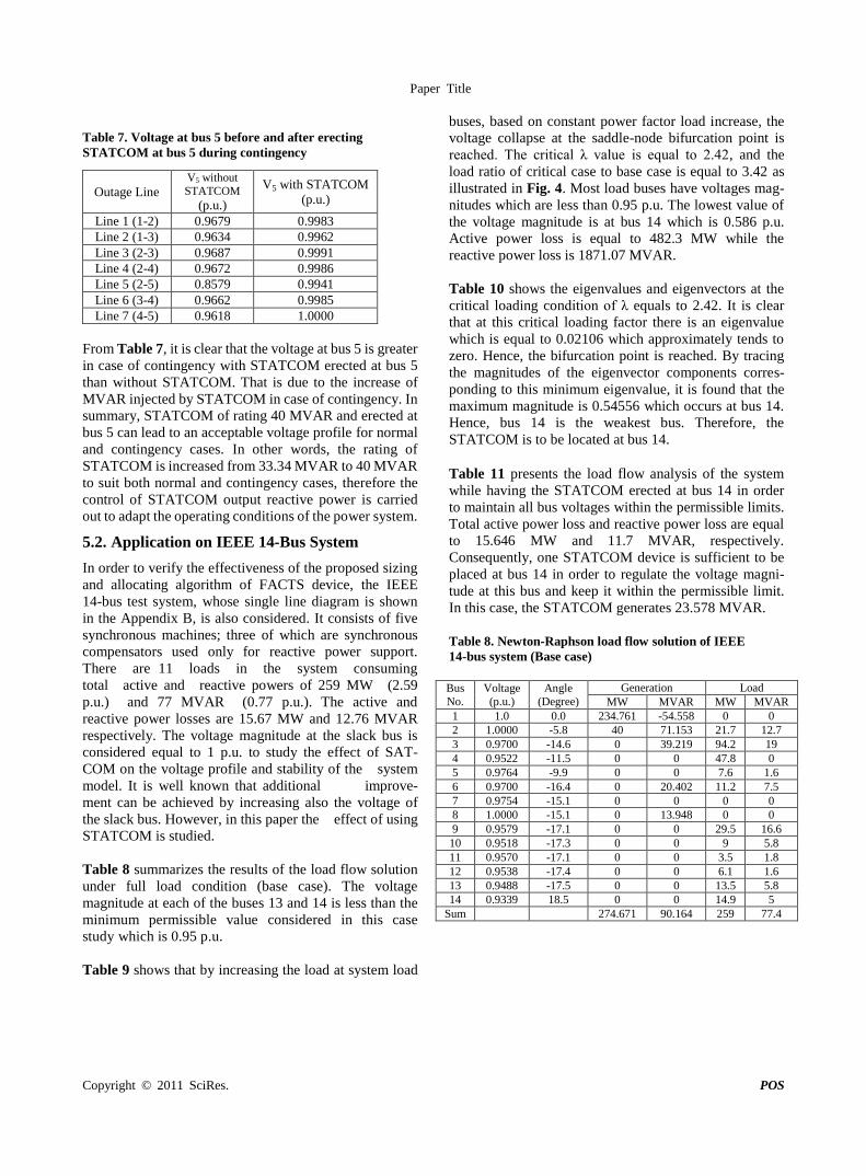
Table 7 illustrates the voltage magnitude at bus 5 before

and after erecting STATCOM at bus 5 during

various cases of contingency.

Table 6. STATCOM rating in MVAR for different line

outages

Line 1 Line 2 Line 3 Line 4 Line 5 Line 6 Line 7

35.42 37.54 34.51 35.03 39.94 35.13 33.87

Load Generation Angle Degree

Voltage (p.u.)

Bus No. MVAR MW MVAR MW

0 0 90.9 761.6 0 1.06 1

39.8 79.6 478.7 40 -18.5 1.00 2

59.7 179.1 0 0 -28.3 0.81 3

19.9 159.2 0 0 1 0.81 4

39.8 238.8 0 0 -36.3 0.78 5

159.2 656.7 569.6 801.6 Sum Eigenvalues

Eigenvectors

Bus 2 Bus

3 Bus 4 Bus 5

50.13 0.011 -0.71 0.70 -0.05

30.98 -0.97 0.10 0.17 0.15

2.19 -0.32 -0.49 -0.53 -0.61

8.67 0.027 -0.48 -0.45 0.75

Paper Title


Table 7. Voltage at bus 5 before and after erecting

STATCOM at bus 5 during contingency

From Table 7, it is clear that the voltage at bus 5 is greater

in case of contingency with STATCOM erected at bus 5

than without STATCOM. That is due to the increase of

MVAR injected by STATCOM in case of contingency. In

summary, STATCOM of rating 40 MVAR and erected at

bus 5 can lead to an acceptable voltage profile for normal

and contingency cases. In other words, the rating of

STATCOM is increased from 33.34 MVAR to 40 MVAR

to suit both normal and contingency cases, therefore the

control of STATCOM output reactive power is carried

out to adapt the operating conditions of the power system.

5.2. Application on IEEE 14-Bus System

In order to verify the effectiveness of the proposed sizing

and allocating algorithm of FACTS device, the IEEE

14-bus test system, whose single line diagram is shown

in the Appendix B, is also considered. It consists of five

synchronous machines; three of which are synchronous

compensators used only for reactive power support.

There are 11 loads in the system consuming

total active and reactive powers of 259 MW (2.59

p.u.) and 77 MVAR (0.77 p.u.). The active and

reactive power losses are 15.67 MW and 12.76 MVAR

respectively. The voltage magnitude at the slack bus is

considered equal to 1 p.u. to study the effect of SAT-

COM on the voltage profile and stability of the system

model. It is well known that additional improve-

ment can be achieved by increasing also the voltage of

the slack bus. However, in this paper the effect of using

STATCOM is studied.

Table 8 summarizes the results of the load flow solution

under full load condition (base case). The voltage

magnitude at each of the buses 13 and 14 is less than the

minimum permissible value considered in this case

study which is 0.95 p.u.

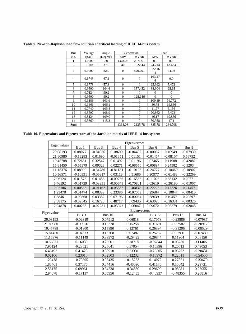
Table 9 shows that by increasing the load at system load

buses, based on constant power factor load increase, the

voltage collapse at the saddle-node bifurcation point is

reached. The critical λ value is equal to 2.42, and the

load ratio of critical case to base case is equal to 3.42 as

illustrated in Fig. 4. Most load buses have voltages mag-

nitudes which are less than 0.95 p.u. The lowest value of

the voltage magnitude is at bus 14 which is 0.586 p.u.

Active power loss is equal to 482.3 MW while the

reactive power loss is 1871.07 MVAR.

Table 10 shows the eigenvalues and eigenvectors at the

critical loading condition of λ equals to 2.42. It is clear

that at this critical loading factor there is an eigenvalue

which is equal to 0.02106 which approximately tends to

zero. Hence, the bifurcation point is reached. By tracing

the magnitudes of the eigenvector components corres-

ponding to this minimum eigenvalue, it is found that the

maximum magnitude is 0.54556 which occurs at bus 14.

Hence, bus 14 is the weakest bus. Therefore, the

STATCOM is to be located at bus 14.

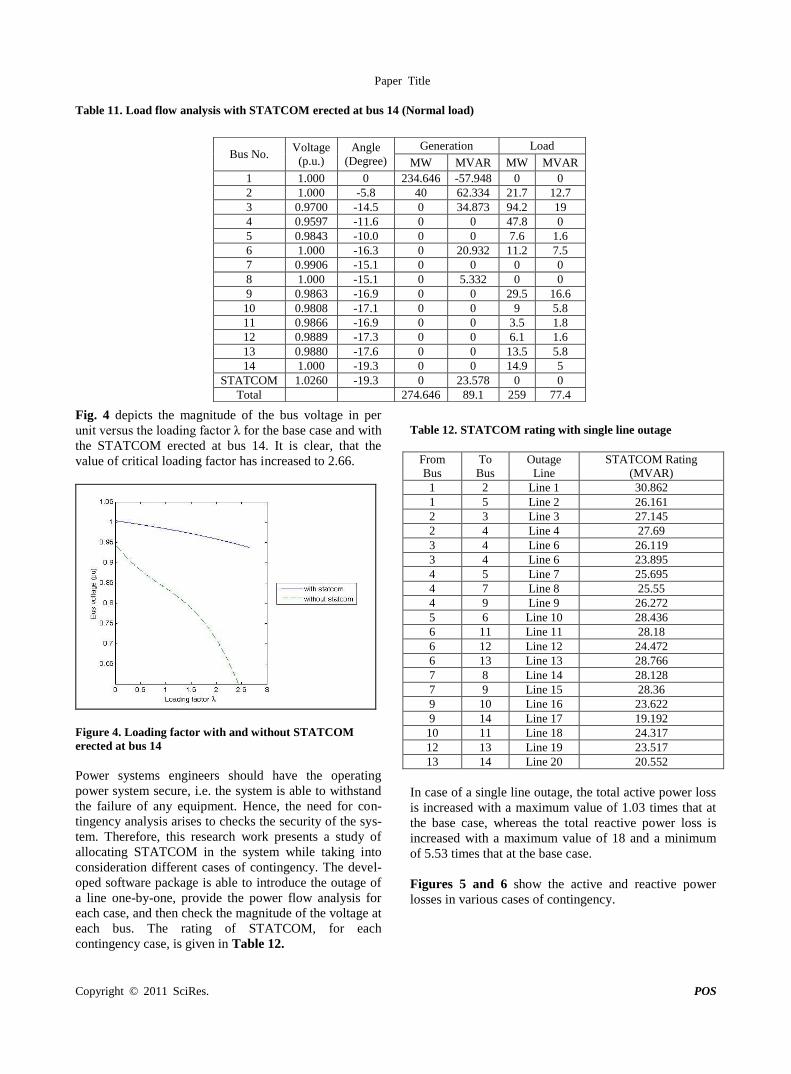
Table 11 presents the load flow analysis of the system

while having the STATCOM erected at bus 14 in order

to maintain all bus voltages within the permissible limits.

Total active power loss and reactive power loss are equal

to 15.646 MW and 11.7 MVAR, respectively.

Consequently, one STATCOM device is sufficient to be

placed at bus 14 in order to regulate the voltage magni-

tude at this bus and keep it within the permissible limit.

In this case, the STATCOM generates 23.578 MVAR.

Table 8. Newton-Raphson load flow solution of IEEE

14-bus system (Base case)


(Degree)

Voltage

(p.u.)

Bus

No. MVAR MW MVAR MW

0 0 -54.558 234.761 0.0 1.0 1

12.7 21.7 71.153 40 -5.8 1.0000 2

19 94.2 39.219 0 -14.6 0.9700 3

0 47.8 0 0 -11.5 0.9522 4

1.6 7.6 0 0 -9.9 0.9764 5

7.5 11.2 20.402 0 -16.4 0.9700 6

0 0 0 0 -15.1 0.9754 7

0 0 13.948 0 -15.1 1.0000 8

16.6 29.5 0 0 -17.1 0.9579 9

5.8 9 0 0 -17.3 0.9518 10

1.8 3.5 0 0 -17.1 0.9570 11

1.6 6.1 0 0 -17.4 0.9538 12

5.8 13.5 0 0 -17.5 0.9488 13

5 14.9 0 0 18.5 0.9339 14

77.4 259 90.164 274.671 Sum

V5 with STATCOM

(p.u.)

V5 without

STATCOM (p.u.)

Outage Line

0.9983 0.9679 Line 1 (1-2)

0.9962 0.9634 Line 2 (1-3)

0.9991 0.9687 Line 3 (2-3)

0.9986 0.9672 Line 4 (2-4)

0.9941 0.8579 Line 5 (2-5)

0.9985 0.9662 Line 6 (3-4)

1.0000 0.9618 Line 7 (4-5)


Table 9. Newton-Raphson load flow solution at critical loading of IEEE 14-bus system


(Degree)

Voltage

(p.u.)

Bus

No. MVAR MW MVAR MW

0.0 0.0 207.061 1328.08 0.0 1.0000 1

43.434 74.214 1022.44 40 -37.0 1.000 2

64.98 322.16

4 420.691 0 -82.0 0.9500 3

0.0 163.47

6 0 0 -67.1 0.6743 4

5.472 25.992 0 0 -57.3 0.6778 5

25.65 38.304 357.452 0 -104.6 0.9500 6

0 0 0 0 -90.2 0.7124 7

0 0 128.146 0 -90.2 0.9500 8

56.772 100.89 0 0 -103.6 0.6189 9

19.836 30.78 0 0 -106.1 0.6361 10

6.156 11.97 0 0 -105.8 0.7740 11

5.472 20.862 0 0 -108.9 0.8597 12

19.836 46.17 0 0 -109.0 0.8124 13

17.1 50.958 0 0 -115.3 0.5860 14

264.708 885.78 2135.78 1368.08 Sum

Table 10. Eigenvalues and Eigenvectors of the Jacobian matrix of IEEE 14-bus system

Eigenvalues Eigenvectors

Bus 1 Bus 3 Bus 4 Bus 5 Bus 6 Bus 7 Bus 8

29.08193 0.08077 -0.84936 0.18699 -0.04492 -0.00067 0.10949 -0.07930

21.80980 -0.13283 0.01690 -0.01851 0.01151 -0.01457 -0.08107 0.58752

19.45788 0.72681 0.32547 0.01492 0.01196 0.02465 0.11908 -0.42082

15.81450 -0.65379 0.09323 0.02271 -0.08550 -0.00897 0.24582 -0.52034

11.15376 0.08909 -0.34786 -0.81181 -0.10108 -0.24777 -0.10460 -0.10902

10.56571 -0.10331 -0.06817 0.03113 0.51685 0.20977 -0.61483 -0.22269

7.96124 0.01573 0.01458 -0.00766 -0.16586 -0.11023 0.35132 0.20771

6.46192 -0.01729 -0.03351 -0.00645 -0.70801 0.02619 -0.26190 -0.01007

0.02106 0.00533 -0.01162 -0.05582 0.40832 -0.22226 0.47226 0.21457

1.23478 -0.01474 0.08333 0.23386 -0.07053 0.29684 -0.18847 -0.08410

1.88461 -0.00868 0.03382 0.07196 -0.00064 0.58039 0.19457 0.20597

2.58175 -0.02545 0.16725 0.48717 0.09435 -0.63020 -0.16331 -0.00326

2.94878 0.00263 -0.02231 -0.05943 0.06047 0.09672 0.05279 -0.02048

Eigenvalues Eigenvectors

Bus 9 Bus 10 Bus 11 Bus 12 Bus 13 Bus 14

29.08193 -0.02319 0.07912 0.06818 0.17078 -0.23886 -0.07987

21.80980 -0.00956 0.16378 0.15258 0.31691 -0.52587 -0.20917

19.45788 -0.01900 0.15890 0.12761 0.26394 -0.31206 -0.08529

15.81450 -0.04633 0.13268 0.07487 0.25257 -0.27931 -0.07489

11.15376 -0.11149 0.33972 -0.29429 0.29844 0.11904 0.08150

10.56571 0.16039 0.25501 0.38718 -0.07844 0.08730 0.11405

7.96124 -0.23521 0.25641 0.57054 -0.15396 0.26613 0.49053

6.46192 0.41423 0.30910 0.23331 -0.25505 0.06772 -0.28431

0.02106 0.23015 0.32503 0.12232 -0.18972 0.22511 -0.54556

1.23478 -0.70805 0.33435 -0.15233 0.14072 0.27871 -0.33670

1.88461 0.37176 0.34416 -0.40090 0.41175 0.15842 0.29731

2.58175 0.09961 0.34238 -0.34550 0.29690 0.08081 0.23055

2.94878 -0.17137 0.35950 -0.12433 -0.48937 -0.48355 0.20816

Paper Title


Table 11. Load flow analysis with STATCOM erected at bus 14 (Normal load)

Fig. 4 depicts the magnitude of the bus voltage in per

unit versus the loading factor λ for the base case and with

the STATCOM erected at bus 14. It is clear, that the

value of critical loading factor has increased to 2.66.

Figure 4. Loading factor with and without STATCOM

erected at bus 14

Power systems engineers should have the operating

power system secure, i.e. the system is able to withstand

the failure of any equipment. Hence, the need for con-

tingency analysis arises to checks the security of the sys-

tem. Therefore, this research work presents a study of

allocating STATCOM in the system while taking into

consideration different cases of contingency. The devel-

oped software package is able to introduce the outage of

a line one-by-one, provide the power flow analysis for

each case, and then check the magnitude of the voltage at

each bus. The rating of STATCOM, for each

contingency case, is given in Table 12.

Table 12. STATCOM rating with single line outage

STATCOM Rating

(MVAR)

Outage

Line

To

Bus

From

Bus

30.862 Line 1 2 1

26.161 Line 2 5 1

27.145 Line 3 3 2

27.69 Line 4 4 2

26.119 Line 6 4 3

23.895 Line 6 4 3

25.695 Line 7 5 4

25.55 Line 8 7 4

26.272 Line 9 9 4

28.436 Line 10 6 5

28.18 Line 11 11 6

24.472 Line 12 12 6

28.766 Line 13 13 6

28.128 Line 14 8 7

28.36 Line 15 9 7

23.622 Line 16 10 9

19.192 Line 17 14 9

24.317 Line 18 11 10

23.517 Line 19 13 12

20.552 Line 20 14 13

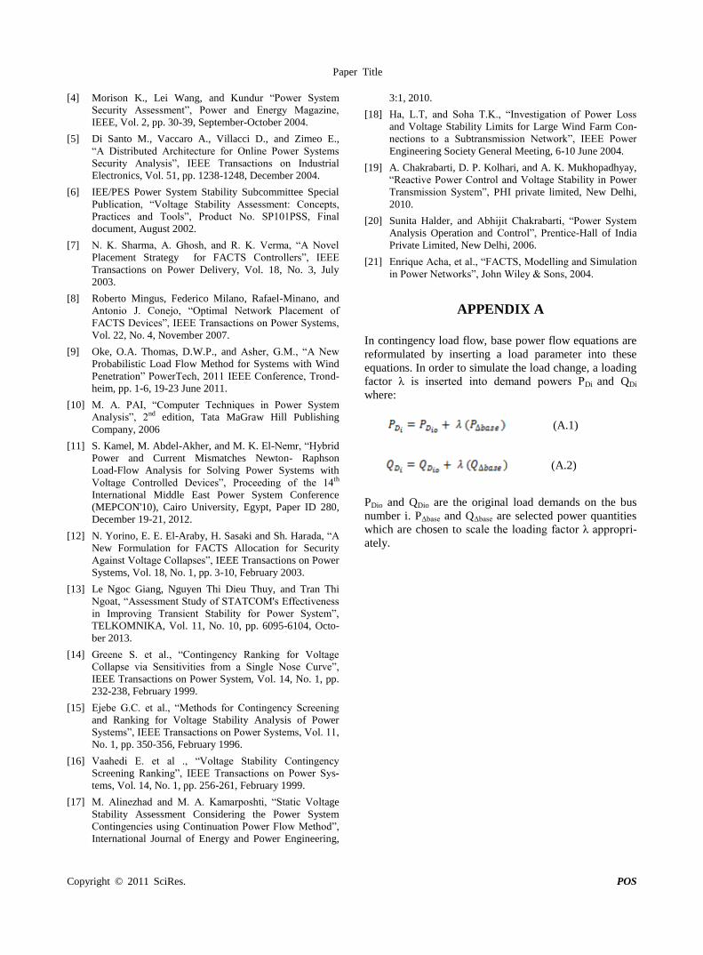
In case of a single line outage, the total active power loss

is increased with a maximum value of 1.03 times that at

the base case, whereas the total reactive power loss is

increased with a maximum value of 18 and a minimum

of 5.53 times that at the base case.

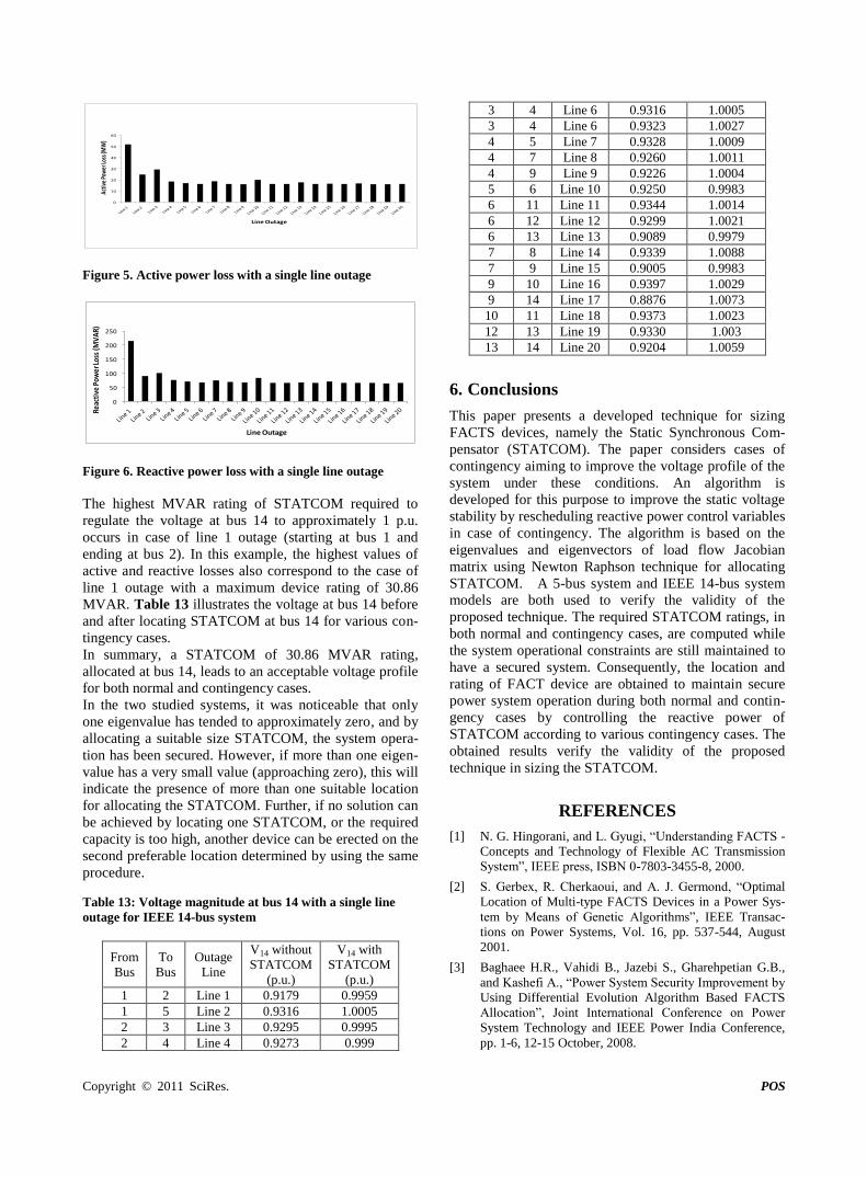
Figures 5 and 6 show the active and reactive power

losses in various cases of contingency.


(Degree)

Voltage

(p.u.) Bus No.

MVAR MW MVAR MW

0 0 -57.948 234.646 0 1.000 1

12.7 21.7 62.334 40 -5.8 1.000 2

19 94.2 34.873 0 -14.5 0.9700 3

0 47.8 0 0 -11.6 0.9597 4

1.6 7.6 0 0 -10.0 0.9843 5

7.5 11.2 20.932 0 -16.3 1.000 6

0 0 0 0 -15.1 0.9906 7

0 0 5.332 0 -15.1 1.000 8

16.6 29.5 0 0 -16.9 0.9863 9

5.8 9 0 0 -17.1 0.9808 10

1.8 3.5 0 0 -16.9 0.9866 11

1.6 6.1 0 0 -17.3 0.9889 12

5.8 13.5 0 0 -17.6 0.9880 13

5 14.9 0 0 -19.3 1.000 14

0 0 23.578 0 -19.3 1.0260 STATCOM

77.4 259 89.1 274.646 Total


0

10

20

30

40

50

60

Activ

e Po

wer

Loss

(MW

)

Line Outage

Figure 5. Active power loss with a single line outage

0

50

100

150

200

250

Reac

tive

Pow

er Lo

ss (M

VA

R)

Line Outage

Figure 6. Reactive power loss with a single line outage

The highest MVAR rating of STATCOM required to

regulate the voltage at bus 14 to approximately 1 p.u.

occurs in case of line 1 outage (starting at bus 1 and

ending at bus 2). In this example, the highest values of

active and reactive losses also correspond to the case of

line 1 outage with a maximum device rating of 30.86

MVAR. Table 13 illustrates the voltage at bus 14 before

and after locating STATCOM at bus 14 for various con-

tingency cases.

In summary, a STATCOM of 30.86 MVAR rating,

allocated at bus 14, leads to an acceptable voltage profile

for both normal and contingency cases.

In the two studied systems, it was noticeable that only

one eigenvalue has tended to approximately zero, and by

allocating a suitable size STATCOM, the system opera-

tion has been secured. However, if more than one eigen-

value has a very small value (approaching zero), this will

indicate the presence of more than one suitable location

for allocating the STATCOM. Further, if no solution can

be achieved by locating one STATCOM, or the required

capacity is too high, another device can be erected on the

second preferable location determined by using the same

procedure.

Table 13: Voltage magnitude at bus 14 with a single line

outage for IEEE 14-bus system

V14 with

STATCOM

(p.u.)

V14 without

STATCOM

(p.u.)

Outage

Line

To

Bus

From

Bus

0.9959 0.9179 Line 1 2 1

1.0005 0.9316 Line 2 5 1

0.9995 0.9295 Line 3 3 2

0.999 0.9273 Line 4 4 2

1.0005 0.9316 Line 6 4 3

1.0027 0.9323 Line 6 4 3

1.0009 0.9328 Line 7 5 4

1.0011 0.9260 Line 8 7 4

1.0004 0.9226 Line 9 9 4

0.9983 0.9250 Line 10 6 5

1.0014 0.9344 Line 11 11 6

1.0021 0.9299 Line 12 12 6

0.9979 0.9089 Line 13 13 6

1.0088 0.9339 Line 14 8 7

0.9983 0.9005 Line 15 9 7

1.0029 0.9397 Line 16 10 9

1.0073 0.8876 Line 17 14 9

1.0023 0.9373 Line 18 11 10

1.003 0.9330 Line 19 13 12

1.0059 0.9204 Line 20 14 13

6. Conclusions

This paper presents a developed technique for sizing

FACTS devices, namely the Static Synchronous Com-

pensator (STATCOM). The paper considers cases of

contingency aiming to improve the voltage profile of the

system under these conditions. An algorithm is

developed for this purpose to improve the static voltage

stability by rescheduling reactive power control variables

in case of contingency. The algorithm is based on the

eigenvalues and eigenvectors of load flow Jacobian

matrix using Newton Raphson technique for allocating

STATCOM. A 5-bus system and IEEE 14-bus system

models are both used to verify the validity of the

proposed technique. The required STATCOM ratings, in

both normal and contingency cases, are computed while

the system operational constraints are still maintained to

have a secured system. Consequently, the location and

rating of FACT device are obtained to maintain secure

power system operation during both normal and contin-

gency cases by controlling the reactive power of

STATCOM according to various contingency cases. The

obtained results verify the validity of the proposed

technique in sizing the STATCOM.

REFERENCES

[1] N. G. Hingorani, and L. Gyugi, “Understanding FACTS -

Concepts and Technology of Flexible AC Transmission

System”, IEEE press, ISBN 0-7803-3455-8, 2000.

[2] S. Gerbex, R. Cherkaoui, and A. J. Germond, “Optimal

Location of Multi-type FACTS Devices in a Power Sys-

tem by Means of Genetic Algorithms”, IEEE Transac-

tions on Power Systems, Vol. 16, pp. 537-544, August

2001.

[3] Baghaee H.R., Vahidi B., Jazebi S., Gharehpetian G.B.,

and Kashefi A., “Power System Security Improvement by

Using Differential Evolution Algorithm Based FACTS

Allocation”, Joint International Conference on Power

System Technology and IEEE Power India Conference,

pp. 1-6, 12-15 October, 2008.

Paper Title


[4] Morison K., Lei Wang, and Kundur “Power System

Security Assessment”, Power and Energy Magazine,

IEEE, Vol. 2, pp. 30-39, September-October 2004.

[5] Di Santo M., Vaccaro A., Villacci D., and Zimeo E.,

“A Distributed Architecture for Online Power Systems

Security Analysis”, IEEE Transactions on Industrial

Electronics, Vol. 51, pp. 1238-1248, December 2004.

[6] IEE/PES Power System Stability Subcommittee Special

Publication, “Voltage Stability Assessment: Concepts,

Practices and Tools”, Product No. SP101PSS, Final

document, August 2002.

[7] N. K. Sharma, A. Ghosh, and R. K. Verma, “A Novel

Placement Strategy for FACTS Controllers”, IEEE

Transactions on Power Delivery, Vol. 18, No. 3, July

2003.

[8] Roberto Mingus, Federico Milano, Rafael-Minano, and

Antonio J. Conejo, “Optimal Network Placement of

FACTS Devices”, IEEE Transactions on Power Systems,

Vol. 22, No. 4, November 2007.

[9] Oke, O.A. Thomas, D.W.P., and Asher, G.M., “A New

Probabilistic Load Flow Method for Systems with Wind

Penetration” PowerTech, 2011 IEEE Conference, Trond-

heim, pp. 1-6, 19-23 June 2011.

[10] M. A. PAI, “Computer Techniques in Power System

Analysis”, 2nd edition, Tata MaGraw Hill Publishing

Company, 2006

[11] S. Kamel, M. Abdel-Akher, and M. K. El-Nemr, “Hybrid

Power and Current Mismatches Newton- Raphson

Load-Flow Analysis for Solving Power Systems with

Voltage Controlled Devices”, Proceeding of the 14th

International Middle East Power System Conference

(MEPCON'10), Cairo University, Egypt, Paper ID 280,

December 19-21, 2012.

[12] N. Yorino, E. E. El-Araby, H. Sasaki and Sh. Harada, “A

New Formulation for FACTS Allocation for Security

Against Voltage Collapses”, IEEE Transactions on Power

Systems, Vol. 18, No. 1, pp. 3-10, February 2003.

[13] Le Ngoc Giang, Nguyen Thi Dieu Thuy, and Tran Thi

Ngoat, “Assessment Study of STATCOM's Effectiveness

in Improving Transient Stability for Power System”,

TELKOMNIKA, Vol. 11, No. 10, pp. 6095-6104, Octo-

ber 2013.

[14] Greene S. et al., “Contingency Ranking for Voltage

Collapse via Sensitivities from a Single Nose Curve”,

IEEE Transactions on Power System, Vol. 14, No. 1, pp.

232-238, February 1999.

[15] Ejebe G.C. et al., “Methods for Contingency Screening

and Ranking for Voltage Stability Analysis of Power

Systems”, IEEE Transactions on Power Systems, Vol. 11,

No. 1, pp. 350-356, February 1996.

[16] Vaahedi E. et al ., “Voltage Stability Contingency

Screening Ranking”, IEEE Transactions on Power Sys-

tems, Vol. 14, No. 1, pp. 256-261, February 1999.

[17] M. Alinezhad and M. A. Kamarposhti, “Static Voltage

Stability Assessment Considering the Power System

Contingencies using Continuation Power Flow Method”,

International Journal of Energy and Power Engineering,

3:1, 2010.

[18] Ha, L.T, and Soha T.K., “Investigation of Power Loss

and Voltage Stability Limits for Large Wind Farm Con-

nections to a Subtransmission Network”, IEEE Power

Engineering Society General Meeting, 6-10 June 2004.

[19] A. Chakrabarti, D. P. Kolhari, and A. K. Mukhopadhyay,

“Reactive Power Control and Voltage Stability in Power

Transmission System”, PHI private limited, New Delhi,

2010.

[20] Sunita Halder, and Abhijit Chakrabarti, “Power System

Analysis Operation and Control”, Prentice-Hall of India

Private Limited, New Delhi, 2006.

[21] Enrique Acha, et al., “FACTS, Modelling and Simulation

in Power Networks”, John Wiley & Sons, 2004.

APPENDIX A

In contingency load flow, base power flow equations are

reformulated by inserting a load parameter into these

equations. In order to simulate the load change, a loading

factor λ is inserted into demand powers PDi and QDi

where:

(A.1)

(A.2)

PDio and QDio are the original load demands on the bus

number i. PΔbase and QΔbase are selected power quantities

which are chosen to scale the loading factor λ appropri-

ately.

Positioning, 2011, *, **

doi:****/pos.2011.***** Published Online ** 2011 (http://www.scirp.org/journal/pos)

APPENDIX B

IEEE 14-bus system model

5-bus system model

Final SGRE paper-Heba-m

Documents