Transitions of income support recipients with Incapacity Exemptions Hielke Buddelmeyer, Yin King Fok, and Ha Vu Melbourne Institute of Applied Economic and Social Research Acknowledgements This research was commissioned by the Australian Government Department of Education, Employment and Workplace Relations (DEEWR) under the Social Policy Research Services Agreement (2005–09) with the Melbourne Institute of Applied Economic and Social Research. The views expressed in this report are those of the authors alone and do not represent those of DEEWR. March 2010 Final Report

Welcome message from author
This document is posted to help you gain knowledge. Please leave a comment to let me know what you think about it! Share it to your friends and learn new things together.
Transcript
Transitions of income support recipients with Incapacity Exemptions
Hielke Buddelmeyer, Yin King Fok, and Ha Vu Melbourne Institute of Applied Economic and Social Research
Acknowledgements This research was commissioned by the Australian Government Department of Education, Employment and Workplace Relations (DEEWR) under the Social Policy Research Services Agreement (2005–09) with the Melbourne Institute of Applied Economic and Social Research. The views expressed in this report are those of the authors alone and do not represent those of DEEWR.
March 2010
Final Report

2
Table of Contents Summary ........................................................................................................................ 3
1. Introduction ............................................................................................................ 6
2. Background ............................................................................................................ 6
2.1. Activity Agreements ........................................................................................ 6
2.2. Activity Test Exemptions ................................................................................ 7
2.3. Temporary Incapacity – Activity Test Exemptions ......................................... 8
2.4. Exemption greater than 26 weeks or medical condition exceeds 13 weeks .... 9
2.5. Continuation of exemption from Activity Test/participation requirements .... 9
2.6. Welfare to Work changes for parents ............................................................ 10
3. Data and definitions ............................................................................................. 11
4. Descriptive Results .............................................................................................. 13
4.1. Time trend in use of TIEs .............................................................................. 13
4.2. The Spell Patterns of UB and TIEs ................................................................ 17
4.3. Distribution of the number of UB and TIE spells per individual .................. 22
4.4. Transitions in Income Support Receipt for Individuals granted TIEs ........... 29
5. Modelling approach ............................................................................................. 37
5.1. The multinomial logit model ......................................................................... 40
5.2. Estimation Results ......................................................................................... 43
6. Concluding remarks ............................................................................................. 50
Appendix ...................................................................................................................... 51
Summary
There are circumstances when a job seeker can be exempt from the Activity Test for a
specified period of time. The use of Temporary Incapacity Exemptions (TIEs) by
unemployment benefit (UB) recipients is the focus of this report, but we also look at the use
of TIEs among individuals on Parenting Payments that are subjected to activity tests. UB
recipients in this report consist of NewStart Allowance (NSA) and Youth Allowance –other
(YAO) recipients.
We find that the main driving force for the time trends of TIE prevalence are the time trends
for NSA recipients with TIEs, as the number of NSA recipients is much larger than the
number of YAO recipients.
The number of UB recipients with TIEs is, overall, declining over time. Four distinct periods
are identified:
July 2002 to July 2003 : number of UB recipients with TIEs is declining
July 2003 to May 2006 : number of UB recipients with TIEs is stable
May 2006 to May 2008 : number of UB recipients with TIEs declines again
May 2008 – onwards : number of UB recipients with TIEs is increasing
The upward trend from May 2008 reflects the impact of the Global Financial Crisis (GFC)
and the subsequent global economic slowdown.
The proportion of UB recipients with a TIE follows the same pattern as the number of UB
recipients with a TIE, with one important exception: the proportion of UB recipients with a
TIE keeps declining uninterrupted from May 2006 onwards. That is, there is no increase in
the proportion of UB recipients with a TIE despite the increase in the number of UB
recipients with a TIE from May 2008 onwards.
The official rule set by Centrelink is that the maximum duration of a TIE is 13 weeks. To
investigate the incidence of consecutively granted TIEs (“extensions”), we combine such
consecutive spells and treat them as a single TIE spell.
4
The distribution of TIE spells is dominated by short spells. More than 80% of all spells last 6
months or less. About 12% of spells last between 6 months and one year with a further 5%
lasting more than one year. The proportion of TIEs lasting one year or more peaked in 2003
and has since declined. TIE spells with durations of 6 months or more, too, declined after
peaking in 2005.
As for timing of TIEs, a high proportion of the TIE spells starts at the beginning of the UB
spell (around 25-30%) with another 10% of spells starting fairly close to the commencement
of the UB spell. There is also a large portion of TIE spells (around 30%) that start after the
recipient has been on UB for a year or more.
As for the TIE incidence, on average, around 20% of the UB spells are observed to have
received at least one TIE at some point. Furthermore, the greater the number of UB spells an
individual has the more likely the individual is observed to have received a TIE.
A comparison of characteristics between UB recipients with and without a TIE showed there
are no major differences between the two groups, except for gender, age and partner status.
▪ A higher proportion of men have had multiple TIE spells, relative to women
▪ UB recipients without TIEs are overrepresented by individuals 25 years of age
or younger, compared to UB recipients with at least one TIE
▪ Among those with multiple TIE spells, singles are overrepresented.
We track UB customers’ benefit receipt status at 6 months, 12 months, and then every year up
to 4 years and distinguish those outcomes by the number of TIE spells customers have within
the first 6 months of their UB spell. The main insights that we find are:
▪ Customers with no TIE experience leave income support at a higher rate than
those with a TIE experience. For example, at the 6-month follow-up point,
36% of the former group have left income support, compared to the equivalent
figure of 27% for the latter group.
▪ The lower rate of leaving income support for the latter group is not translated
into their rate of remaining on UB: the rates of staying on UB for both groups
are fairly similar. Rather, the difference is observed in the rate of transferring
5
to other payments, especially to the DSP program. Those who had received a
TIE were much more likely to have transferred to DSP, compared to those who
did not.
Economic modelling described the probability, at the one-year follow-up mark, to be
observed on UB, on DSP, on any other income support payment, or off income support. It
showed:
▪ Experiencing a TIE in the first 6 months of an UB spell is associated with a
reduction of 10 percentage points in the probability of having left income
support one year later.
▪ Having one TIE spell (relative to none) in the first 6 months of an UB spell
increases the probability of being observed on DSP at the 12 month follow-up
by 3 percentage points. Having multiple TIE spells increases the probability of
remaining on UB by 7.3%.
▪ When we restrict our sample for the analysis to UB spells that lasted 12
months or more, having a TIE spell during the initial 12 month since UB spell
commencement reduced the probability of being off income support at the one-
year follow-up by about 6 percentage points. This is significantly smaller than
the comparable effects for the case of the initial UB spell period of 6 months.
6
1. Introduction
Income support recipients on activities-tested payments are able to obtain an exemption from
Centrelink if they are unable to meet their participation (i.e. activity test) requirements. While
each income support payment may have specific types of exemptions, the research presented
in this report is restricted to temporary incapacity exemptions (TIEs) granted to income
support customers on the following payment types: Unemployment Benefit (UB) and
Parenting Payments (PP) that are subject to activity tests. UB includes Newstart Allowance
(NSA) and Youth Allowance Other (YAO) and Parenting Payments (PP) that are subject to
activity tests include Parenting Payment Single (PPS) and Parenting Payment Partnered
(PPP).
Specifically, this report answers the following three questions:
[1] What are the characteristics of recipients that are granted TIEs?
[2] What is the likelihood of recipients granted a TIE ending up more isolated because of
transfers to income support payment with no participation requirements?
[3] What are the time trends in relation to TIE prevalence?
The report proceeds as follows. Section 2 outlines the background information on activity
agreements and temporary incapacity exemptions, and discusses the welfare to work changes
for parents in relation to participation requirements. In section 3, we provide a brief
description on how the RED data is used in the research and our approach to sample selection.
Section 4 present descriptive results and Section 5 outlines our modelling approach and
presents findings from the estimations. Section 6 concludes.
2. Background
2.1. Activity Agreements
Up until 1 July 2009, certain customers were required to enter into an Activity Agreement
(AA) with an employment service provider in order to continue to receive their payments.1
1 The AA has since been replaced by the Employment Pathway Plan (EPP). Since our time span of the data in this report is pre-1 July 2009 we will limit our discussion to the role of the AA.
7
Customers were expected to undertake the compulsory activities included in their AA. If they
failed to undertake the activities as outlined in the agreement, a participation failure or serious
failure may have been committed.
The AA contained both compulsory activities that the job seeker had to complete as well as
voluntary activities that the job seeker chose to undertake. When the AA was negotiated, all
activities were considered to ensure that the final agreement was appropriate for the customer.
All activities selected for inclusion in the AA were presented to the customer in a consistent
format, which clearly identifies compulsory and voluntary requirements. The AA was printed,
signed and given to the customer each time it was negotiated or updated. The key features of
an AA were:
o Centrelink added activities that a job seeker must complete to satisfy the Activity Test
or their participation requirements
o Job Network Members (JNMs) added activities to assist the job seeker in finding work
o Community Work Coordinators (CWCs) added Work for the Dole (WFD) and
Community Work requirements
o Disability Employment Network (DEN) providers added activities relating to
disability
o Providers of other programs such as Personal Support Programme (PSP), Vocational
Rehabilitation Services (VRS) and Job Placement, Employment and Training (JPET)
2.2. Activity Test Exemptions
Job seekers in receipt of NSA, Youth Allowance (YA) or Parenting Payment (PP) with a
participation requirement are required to participate in the Activity Test to remain qualified
for payments. There are circumstances when a job seeker can be exempt from the Activity
Test for a specified period of time. The full details of different customers being exempt based
on specific circumstances will not be discussed here2
2 The Social Security Guide, section 3.2.12, provides specific details on the various types of activity test exemptions, but the exemptions are granted for: Temporary Incapacity; Pregnancy; Remote Areas; Special
, with one exception (as it is the focus of
this report): Temporary Incapacity.

8
2.3. Temporary Incapacity – Activity Test Exemptions
A job seeker claiming or receiving NSA, YA, PP, or in some cases Special Benefit (SpB),
may request an exemption from the Activity Test/participation requirements by lodging an
'approved' medical certificate. For the purposes of an exemption from the Activity Test, a
person has a temporary incapacity for work or study if they have an illness, injury or
disability that is, or is likely to be, of a temporary3
o undertaking work of eight hours or more in a week at or above the relevant minimum
wage, which the person could reasonably be expected to do if they were not
incapacitated, or
nature and which prevents them from:
o unable to continue the course of study they were doing before they became
incapacitated
And:
o they are unable to undertake another activity deemed suitable by the Secretary, and
o they provide a medical certificate that states
o the medical practitioner's diagnosis,
o the medical practitioner's prognosis that they are incapacitated for work or
study, and
o the period of the incapacity
And:
o The incapacity was not brought about with the view to obtaining an exemption from
the activity test.
Circumstances; Principal Carer Parents with Special Family Circumstances (Automatic and Case-by-Case); and Partial Capacity to Work 3 An incapacity for work or study is considered to be temporary if it is likely that the customer will be able to return to work or study within the next two years. However, it is generally expected that a customer will be able to return to work, or look for work, in a shorter period of time.

9
Where the customer meets the eligibility criteria for a temporary incapacity exemption, the
incapacity exemption period will be for the duration stated on the medical certificate or 13
weeks from the start date of the medical certificate (whichever is shorter).
Note that lodgement of a medical certificate does not automatically result in an exemption
being granted. If the customer's capacity to work is eight hours or more per week, but less
than 30 hours per week, an incapacity exemption is not granted. This is because they can
satisfy Activity Test/participation requirements, but may have required a modified AA that
takes into account their current circumstances. Similarly, a customer may be unable to work at
least 8 hours, yet not qualify for an incapacity exemption because they are still able to
participate in a suitable activity, i.e. take part in services or other activities to help them
prepare for a job. Where an exemption is not granted (despite the medical certificate
lodgement) the customer will be subject to Activity Test/participation requirements, taking
the customer's current work capacity into consideration.
2.4. Exemption greater than 26 weeks or medical condition exceeds 13 weeks
If a customer is about to reach more than 26 weeks on an incapacity exemption or their
medical condition will exceed 13 weeks, and they are:
o undergoing or recovering from radiotherapy or chemotherapy
o about to undergo major surgery such as joint replacement, organ transplant or heart
surgery
o recovering from major surgery such as joint replacement, organ transplant or heart
surgery,
the conversation had with the customer will be documented as to the expected date for
surgery or the date when the surgery took place; anticipated recovery time frame and dates for
follow-up as necessary.
2.5. Continuation of exemption from Activity Test/participation requirements

10
The period of exemption from Activity Test/participation requirements can be extended if
there are no changes to the customer's circumstances on which the initial period of exemption
was granted. That is:
o the new medical certificate must show that the job seeker is temporarily incapacitated
for all work (8 hours per week or more), and
o The job seeker is still unable to undertake any suitable activity that will increase their
level of participation.
Customers who lodge a medical certificate will not automatically have an exemption from
Activity Test/participation requirements approved; rather their capacity to work or participate
in a suitable activity is re-assessed. An assessment of the customer's work capacity is required
to inform appropriate intervention and support necessary to address the person's barriers to
participation if a further exemption based on the new medical certificate would mean that the
job seeker will have a total of more than 26 weeks incapacity exemption in a 12-month period
(including future periods). If available, a current and valid JCA should be used for this. If
there is no current and valid assessment, a referral for a JCA must be made.
2.6. Welfare to Work changes for parents
Building on the previous policy changes introduced as part of Australians Working Together
and information gathered from consultations and pilot programs, the Australian Government
in July 2006 introduced comprehensive changes to the welfare system for working age
Australians, to bring it more in line with community norms and the changed economic
conditions. Parenting Payment remained available to eligible parents with children aged up to
6 years of age. Parents with a youngest child aged less than 6 years of age did not have any
job search requirements. However, once their youngest child was school-aged parents were
generally considered to have capacity to engage with the labour market on a part-time basis.
Under Welfare to Work, principal carer parents who claimed PP on or after 1 July 2006
received this payment until their youngest child turned 6 (if partnered) or 8 (if single). After
this time, they needed to apply for another income support payment (typically NSA or
Austudy) and meet part-time participation requirements. Both single and partnered parents
had part-time participation requirements once their youngest child turned 6.
11
Parents who were receiving PP before 1 July 2006 continued to receive their payment until
their youngest child turned 16, as long as they remained eligible. From 1 July 2007, parents
from this ‘grandfathered’ group with a youngest child 7 and over were required to meet part-
time participation requirements.4
Parents with participation requirements did not have to accept jobs that were unsuitable. For a
job to be considered suitable, parents required access to appropriate care and supervision for
their children at the times when they would be required to undertake the work. Further, they
were not required to accept or continue in a job if the principal carer parent was not at least
$50 a fortnight better off after the costs of employment such as child care were taken into
account (compared to not working), or if travel time to work was more than 60 minutes each
way (including the time to drop a child at child care or school) or was too expensive.
To summarise, principle carers whose child is less than 6 years of age never have a
participation requirement. Customers who came onto PP on or after 1 July 2006 had a
participation requirement as soon as their youngest child turned 6 years of age. Furthermore,
single customers would transfer to another income support payment (typically NSA or
Austudy) once their youngest child turned 8 years of age. Partnered customers would transfer
to another income support payment (typically NSA or Austudy) once their youngest child
turned 6 (in effect their participation requirement when their youngest child turns 6 coincides
with their ineligibility for PP).
Customers who were receiving PP before 1 July 2006 could stay on PP until their youngest
child turned 16 years of age. However, from 1 July 2007 (a year after the changes) this
grandfathered group had a part time requirement once their youngest child turned 7 years of
age.
3. Data and definitions
The data used in this report come from the Research and Evaluation Dataset (RED), extracted
in August 2009. The data period ends in 30 June 2009 and in this paper, we focus our analysis
on the period from 1 July 2002 to 30 June 2009 for the UB sample and 1 July 2006 to 30 June 4 Protections were in place for parents in certain groups who did not have the capacity to engage with the labour market. Exemptions were available for registered and active foster carers, relatives caring for a child under the family law order, those undertaking home schooling, distance education or those with a large family (four or more children aged under 16). All single parents on NSA who were exempt from participation requirements due to the above reasons received a maximum allowance rate equivalent to the Parenting Payment single rate.

12
2009 for the PP sample. We will first discuss the UB sample before discussing the
construction of the PP sample.
The main tables used are the BENHIST and MEDICAL_DETAILS tables. As a first step, and
in order to focus on the first main research question outlined in Section 1, we took a 1%
random sample of the pool of customers who, at some point during the time span from July
2002 to June 2009, were in receipt of UB. This resulted in a sample of 28,934 individuals
denoted as the ‘1% UB Sample’. Next, using the table MEDICAL_DETAILS, we constructed
episodes of TIEs using the start and end dates of the medical certificates denoted by
‘smedc_cert_start_date’ and ‘smedc_cert_end_date’, respectively. Both the UB episodes and
TIE episodes were merged into a single file so that for each fortnight that a customer was in
receipt of UB, it would be known if he/she was also granted a TIE or not. In a final step some
personal characteristics from the CUSTOMER, PARTNER, ISS CHILDREN, and
POSTCODE tables were merged into this file for the descriptive and multivariate analyses.
All tables, figures and results from economic modelling are based on this 1% UB Sample.
For our PP sample we use data from the post Welfare to Work (WtW) period 1 July 2006 to
30 June 2009. Information on whether individuals on parenting payments are subject to
activity tests or not is derived from the TARGPCAR table using the variable pc_subcat_code.
This variable identifies, for each spell of parenting payment, the two aspects that determine
whether the individual has an activity test requirement or not: whether the individual was a
new entrant on this type of welfare after the implementation of the WtW policy and the age
group that their youngest belong to.
Similar to the procedure used for UB recipients, but catering for the fact that a much lower
number of individuals would have been on activity tested Parenting Payments (ATPP) relative
to UB, we took a 10% random sample of primary care applicants who had been on either
Parenting Payment Single (PPS) or Parenting Payment Partnered (PPP) at some point during
the period 1 July 2006 to 30 June 2009. This resulted in a sample of 83,884 individuals,
among which 32,237 individuals had been subjected to activity tests at some point during the
observation window. The rest of the data construction procedure proceeded in an identical
manner to that already discussed for the UB section. That is, details from the BENHIST,
MEDICAL_DETAILS, CUSTOMER, PARTNER, ISS CHILDREN, and POSTCODE tables
were merged into the file containing PP episodes to create a dataset containing fortnightly
information on individuals’ characteristics, income support and TIE status.
13
4. Descriptive Results
4.1. Time trend in use of TIEs
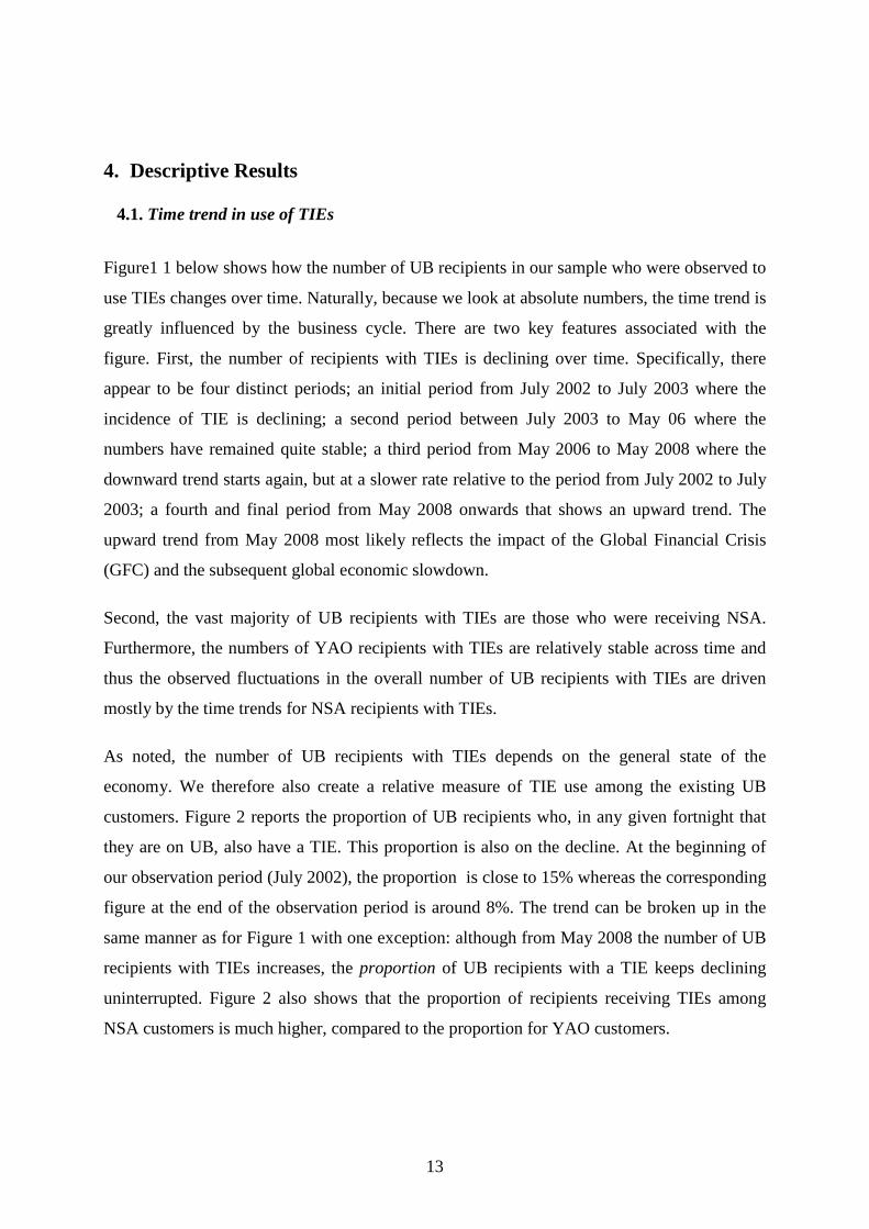
Figure1 1 below shows how the number of UB recipients in our sample who were observed to
use TIEs changes over time. Naturally, because we look at absolute numbers, the time trend is
greatly influenced by the business cycle. There are two key features associated with the
figure. First, the number of recipients with TIEs is declining over time. Specifically, there
appear to be four distinct periods; an initial period from July 2002 to July 2003 where the
incidence of TIE is declining; a second period between July 2003 to May 06 where the
numbers have remained quite stable; a third period from May 2006 to May 2008 where the
downward trend starts again, but at a slower rate relative to the period from July 2002 to July
2003; a fourth and final period from May 2008 onwards that shows an upward trend. The
upward trend from May 2008 most likely reflects the impact of the Global Financial Crisis
(GFC) and the subsequent global economic slowdown.
Second, the vast majority of UB recipients with TIEs are those who were receiving NSA.
Furthermore, the numbers of YAO recipients with TIEs are relatively stable across time and
thus the observed fluctuations in the overall number of UB recipients with TIEs are driven
mostly by the time trends for NSA recipients with TIEs.
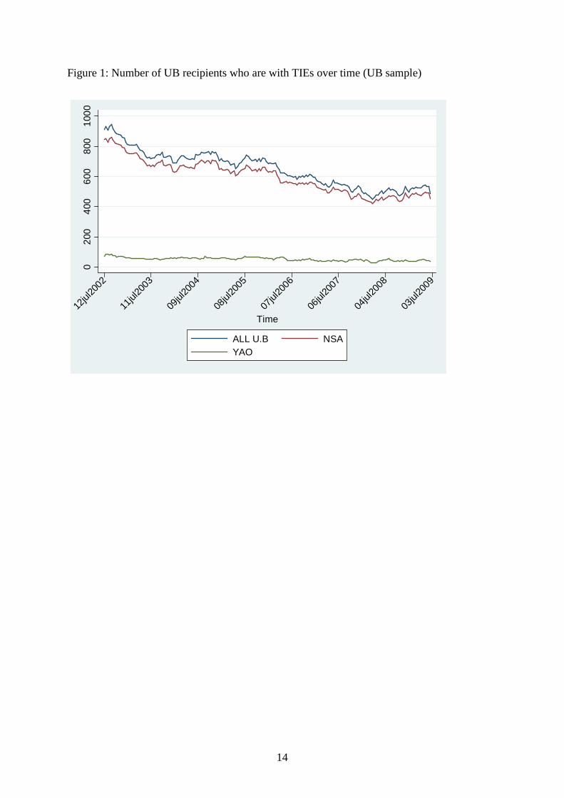
As noted, the number of UB recipients with TIEs depends on the general state of the
economy. We therefore also create a relative measure of TIE use among the existing UB
customers. Figure 2 reports the proportion of UB recipients who, in any given fortnight that
they are on UB, also have a TIE. This proportion is also on the decline. At the beginning of
our observation period (July 2002), the proportion is close to 15% whereas the corresponding
figure at the end of the observation period is around 8%. The trend can be broken up in the
same manner as for Figure 1 with one exception: although from May 2008 the number of UB
recipients with TIEs increases, the proportion of UB recipients with a TIE keeps declining
uninterrupted. Figure 2 also shows that the proportion of recipients receiving TIEs among
NSA customers is much higher, compared to the proportion for YAO customers.
14
Figure 1: Number of UB recipients who are with TIEs over time (UB sample) 0
200
400
600
800
1000
12jul
2002
11jul
2003
09jul
2004
08jul
2005
07jul
2006
06jul
2007
04jul
2008
03jul
2009
Time
ALL U.B NSAYAO
15
Figure 2: Proportion of all existing UB recipients with TIEs over time (UB sample) .0
5.1
.15
12jul
2002
11jul
2003
09jul
2004
08jul
2005
07jul
2006
06jul
2007
04jul
2008
03jul
2009
Time
ALL U.B NSAYAO
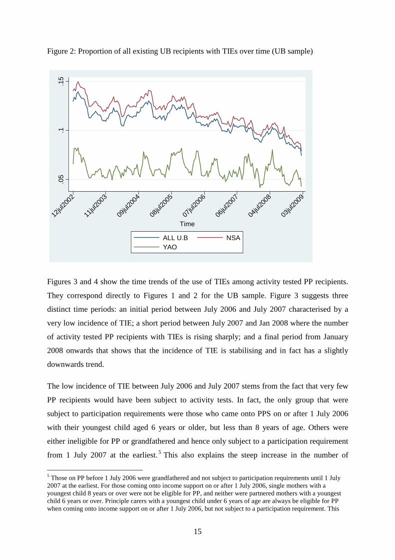
Figures 3 and 4 show the time trends of the use of TIEs among activity tested PP recipients.
They correspond directly to Figures 1 and 2 for the UB sample. Figure 3 suggests three
distinct time periods: an initial period between July 2006 and July 2007 characterised by a
very low incidence of TIE; a short period between July 2007 and Jan 2008 where the number
of activity tested PP recipients with TIEs is rising sharply; and a final period from January
2008 onwards that shows that the incidence of TIE is stabilising and in fact has a slightly
downwards trend.
The low incidence of TIE between July 2006 and July 2007 stems from the fact that very few
PP recipients would have been subject to activity tests. In fact, the only group that were
subject to participation requirements were those who came onto PPS on or after 1 July 2006
with their youngest child aged 6 years or older, but less than 8 years of age. Others were
either ineligible for PP or grandfathered and hence only subject to a participation requirement
from 1 July 2007 at the earliest. 5
5 Those on PP before 1 July 2006 were grandfathered and not subject to participation requirements until 1 July 2007 at the earliest. For those coming onto income support on or after 1 July 2006, single mothers with a youngest child 8 years or over were not be eligible for PP, and neither were partnered mothers with a youngest child 6 years or over. Principle carers with a youngest child under 6 years of age are always be eligible for PP when coming onto income support on or after 1 July 2006, but not subject to a participation requirement. This
This also explains the steep increase in the number of
16
recipients with TIEs from 1 July 2007 onwards as those PP recipients with children aged 6 or
over that were grandfathered now become subject to participation requirements. However, the
overall pattern of TIE incidences over time is very much driven by PPS.
Figure 4 shows the proportion of TIE use among all ATPP recipients. Because the ATPP is
dominated by PPS the lines for all PP and PPS are very close. Note that they do (and should)
overlap for the period 1 July 2006 and 1 July 2007 because no PPP recipient could be subject
to participation requirements during that time frame as explained when discussing Figure 3
(specifically in footnote 5). However, one has to keep in mind that during this period there are
only very few PPS recipients that are subject to activity tests and that as a result the
proportion with a TIE can be quite volatile.
Figure 3: Number of activity tested PP recipients who are with TIEs over time (ATPP sample)
050
010
0015
00
07jul
2006
05jan
2007
06jul
2007
04jan
2008
04jul
2008
02jan
2009
03jul
2009
Time
ALL activity tested PP PPPPPS
leaves single mothers on PPS with a child between 6 and 8 years of age, and who were not grandfathered, as the only group on PP subject to participation requirements for the period 1 July 2006 to 1 July 2007.

17
Figure 4: Proportion of all existing activity tested PP recipients with TIEs over time (ATPP
sample) 0
.02
.04
.06
.08
07jul
2006
05jan
2007
06jul
2007
04jan
2008
04jul
2008
02jan
2009
03jul
2009
Time
ALL activity tested PP PPPPPS
4.2. The Spell Patterns of UB and TIEs
Table 1 describes the distribution of the UB spells commenced within the period starting from
July 2002 to December 2008. We produce this distribution of spell lengths by year of spell
commencement. It is important to note that for some of the UB spells starting in 2006 or
later, it is not possible to determine their duration since the individuals are still receiving UB
at the end of the observation window. These spells are identified by the missing cells in the
table. They are termed right censored spells in which the outcome, exit from unemployment
benefits in this case, is not yet observed.
As it is shown in the table, the spell distribution is very stable across the years. The
distribution is dominated by short spells, with close to three quarters of all spells lasting 6
months or less. About 12% of spells last between 1 and 2 years with a further 10% lasting
more than 2 years.

18
Table 1: Distribution of UB spell durations by year spell started (UB sample)
UB spell started in Duration 2002 2003 2004 2005 2006 2007 2008 less one month 10.55 9.42 9.14 9.33 9.52 10.59 10.51 1-3 months 24.00 24.42 23.04 23.65 24.4 23.52 21.33 3-6 months 23.34 25.04 25.59 24.86 26.26 26.33 22.58 half to one year 19.83 19.14 19.99 20.26 18.29 17.82 - 1-2 years 12.01 12.42 12.23 12.28 (a)- - - 2years+ 10.27 9.56 10.02 9.62 - - - Total 3,904 6,942 6,609 6,432 6,062 5,864 6,062
Notes: (a) the missing cells relate to those spells starting later in the observation period for which the duration interval cannot be determined due to right censoring (i.e. they were still ongoing when the observation period ended).
Multiple spells for the same customer are treated as individual spells.
Table 2 below describes the distribution of the TIE spells commenced between July 2002 and
December 2008 for the UB sample. It is important to note that a single UB spell can have
multiple TIE spells, and where there are multiple TIEs granted consecutively they are treated
as a single continuous TIE spell for the purpose of duration determination. This allows us to
obtain an estimate of the extent to which customers make use of consecutive exemptions.
Hence, the duration of a TIE spell can be much larger than the maximum duration of 13
weeks.
Table 2 shows that there are a significant number of individuals who have TIE spells with
durations that are greater than 13 weeks, suggesting that many of them have applied for
multiple TIEs (extensions). The distribution of the TIE spells that commenced within our
observation window is dominated by short spells, with around 80% of all spells lasting 6
months or less. About 12% of spells last between 6 months and one year with a further 5%
lasting more than one year. With regard to time trends, the spell distribution across years is
more or less constant, albeit that the proportion of TIEs with a duration of one year or more
peaked in 2003 and has since declined. Similarly, spells lasting 6 months or more have
declined after peaking in 2005.

19
Table 2: Distribution of TIE spell durations by year TIE spell started (UB sample)
TIE spell started in Duration 2002 2003 2004 2005 2006 2007 2008
Less then one
fortnights 11.22 10.55 10.05 8.33 8.42 10.35 10.4 2 fortnights 13.82 11.86 13.73 12.65 13.76 13.3 14.02 3 fortnights 12.3 11.71 11.2 11.91 12.24 13.41 11.37 4 fortnights 6.73 7.47 7.66 7.84 7.8 8.34 8.88 5 fortnights 6.37 6.92 7.85 7.94 8.22 8.45 7.26 6 fortnights 5.83 4.8 4.59 5.83 6.02 5.89 7.2 7 fortnights 9.25 10.25 9.47 9.71 10.05 10.41 10.5 8 fortnights 6.55 7.32 7.08 7.3 7.17 6.92 7.31 9 fortnights 2.24 2.78 2.49 2.6 2.51 1.69 2.98
10 fortnights 2.06 2.47 1.91 2.4 2.15 2.56 2.65 11 fortnights 1.71 1.31 1.53 1.52 2.09 1.42 1.68 12 fortnights 2.33 1.82 2.25 1.72 2.15 2.23 1.95 13 fortnights 1.71 2.07 1.96 2.16 2.51 2.18 (a)-
half to one year 12.12 11.96 12.39 13.58 11.15 10.52 - one year+ 5.75 6.71 5.84 4.51 3.77 2.34 - Total number of spells 1,114 1,981 2,090 2,040 1,911 1,835 1,847
Notes: (a) the missing cells relate to those spells starting later in the observation period for which the duration cannot be determined due to right censoring (i.e. they were still ongoing when the observation period ended).
Consecutive TIE spells (i.e. extensions) are treated as a single TIE spell (hence durations that exceed 13 weeks).
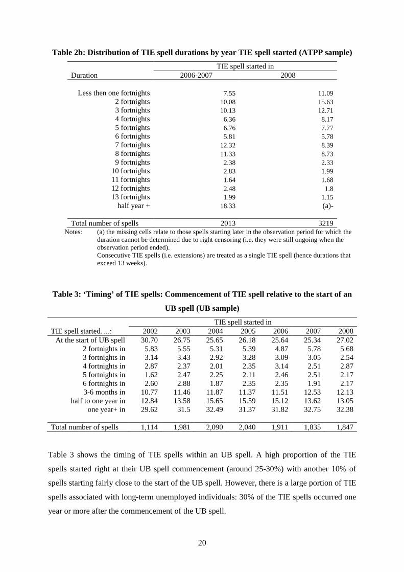
Table 2b describes the distribution of the TIE spells commenced between July 2006 and
December 2008 for our ATPP sample. Due to the low numbers of ATPP recipients (and hence
TIEs) in 2006 we combine the TIE spells that start in 2006 and 2007. For those TIE spells the
most common durations are 2 or 3, 7 or 8, or more than 13 fortnights.
20
Table 2b: Distribution of TIE spell durations by year TIE spell started (ATPP sample)
TIE spell started in Duration 2006-2007 2008
Less then one fortnights 7.55 11.09 2 fortnights 10.08 15.63 3 fortnights 10.13 12.71 4 fortnights 6.36 8.17 5 fortnights 6.76 7.77 6 fortnights 5.81 5.78 7 fortnights 12.32 8.39 8 fortnights 11.33 8.73 9 fortnights 2.38 2.33
10 fortnights 2.83 1.99 11 fortnights 1.64 1.68 12 fortnights 2.48 1.8 13 fortnights 1.99 1.15
half year + 18.33 (a)- Total number of spells 2013 3219
Notes: (a) the missing cells relate to those spells starting later in the observation period for which the duration cannot be determined due to right censoring (i.e. they were still ongoing when the observation period ended).
Consecutive TIE spells (i.e. extensions) are treated as a single TIE spell (hence durations that exceed 13 weeks).
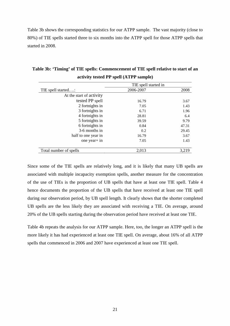
Table 3: ‘Timing’ of TIE spells: Commencement of TIE spell relative to the start of an
UB spell (UB sample)
TIE spell started in TIE spell started….: 2002 2003 2004 2005 2006 2007 2008
At the start of UB spell 30.70 26.75 25.65 26.18 25.64 25.34 27.02 2 fortnights in 5.83 5.55 5.31 5.39 4.87 5.78 5.68 3 fortnights in 3.14 3.43 2.92 3.28 3.09 3.05 2.54 4 fortnights in 2.87 2.37 2.01 2.35 3.14 2.51 2.87 5 fortnights in 1.62 2.47 2.25 2.11 2.46 2.51 2.17 6 fortnights in 2.60 2.88 1.87 2.35 2.35 1.91 2.17 3-6 months in 10.77 11.46 11.87 11.37 11.51 12.53 12.13
half to one year in 12.84 13.58 15.65 15.59 15.12 13.62 13.05 one year+ in 29.62 31.5 32.49 31.37 31.82 32.75 32.38
Total number of spells 1,114 1,981 2,090 2,040 1,911 1,835 1,847
Table 3 shows the timing of TIE spells within an UB spell. A high proportion of the TIE
spells started right at their UB spell commencement (around 25-30%) with another 10% of
spells starting fairly close to the start of the UB spell. However, there is a large portion of TIE
spells associated with long-term unemployed individuals: 30% of the TIE spells occurred one
year or more after the commencement of the UB spell.
21
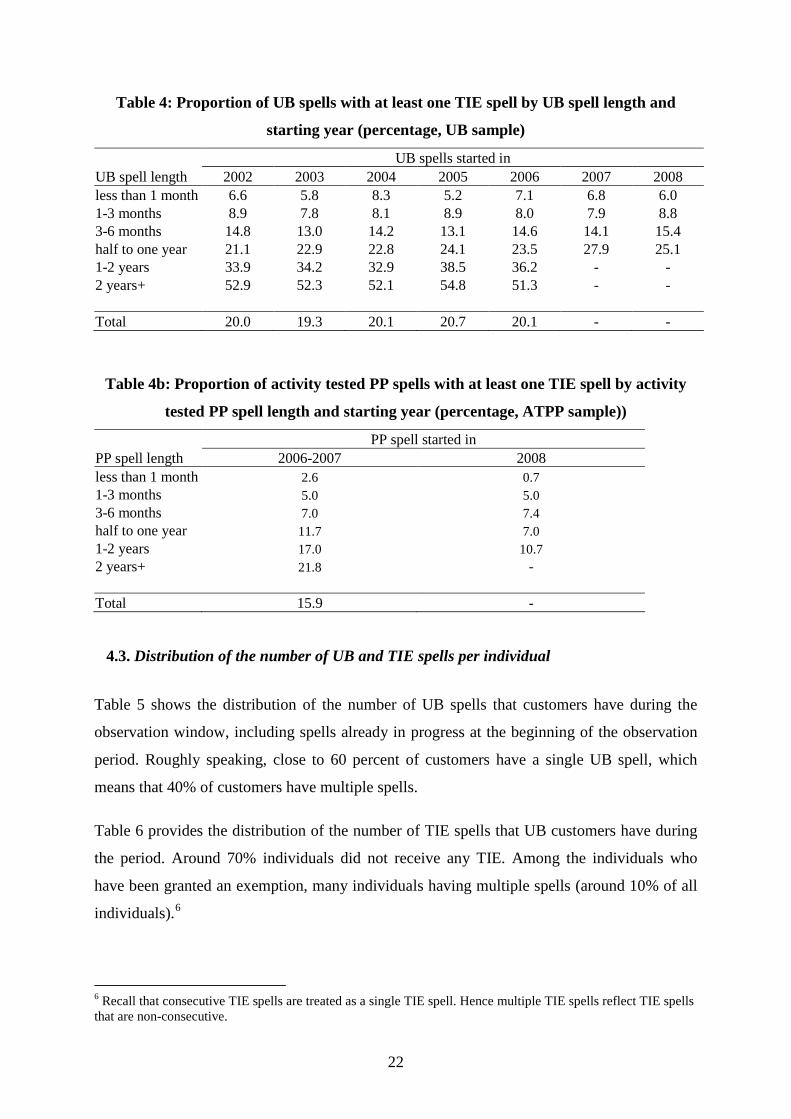
Table 3b shows the corresponding statistics for our ATPP sample. The vast majority (close to
80%) of TIE spells started three to six months into the ATPP spell for those ATPP spells that
started in 2008.
Table 3b: ‘Timing’ of TIE spells: Commencement of TIE spell relative to start of an
activity tested PP spell (ATPP sample)
TIE spell started in TIE spell started….: 2006-2007 2008
At the start of activity tested PP spell 16.79 3.67
2 fortnights in 7.05 1.43 3 fortnights in 6.71 1.96 4 fortnights in 28.81 6.4 5 fortnights in 39.59 9.79 6 fortnights in 0.84 47.31 3-6 months in 0.2 29.45
half to one year in 16.79 3.67 one year+ in 7.05 1.43
Total number of spells 2,013 3,219
Since some of the TIE spells are relatively long, and it is likely that many UB spells are
associated with multiple incapacity exemption spells, another measure for the concentration
of the use of TIEs is the proportion of UB spells that have at least one TIE spell. Table 4
hence documents the proportion of the UB spells that have received at least one TIE spell
during our observation period, by UB spell length. It clearly shows that the shorter completed
UB spells are the less likely they are associated with receiving a TIE. On average, around
20% of the UB spells starting during the observation period have received at least one TIE.
Table 4b repeats the analysis for our ATPP sample. Here, too, the longer an ATPP spell is the
more likely it has had experienced at least one TIE spell. On average, about 16% of all ATPP
spells that commenced in 2006 and 2007 have experienced at least one TIE spell.
22
Table 4: Proportion of UB spells with at least one TIE spell by UB spell length and
starting year (percentage, UB sample)
UB spells started in UB spell length 2002 2003 2004 2005 2006 2007 2008 less than 1 month 6.6 5.8 8.3 5.2 7.1 6.8 6.0 1-3 months 8.9 7.8 8.1 8.9 8.0 7.9 8.8 3-6 months 14.8 13.0 14.2 13.1 14.6 14.1 15.4 half to one year 21.1 22.9 22.8 24.1 23.5 27.9 25.1 1-2 years 33.9 34.2 32.9 38.5 36.2 - - 2 years+ 52.9 52.3 52.1 54.8 51.3 - -
Total 20.0 19.3 20.1 20.7 20.1 - -
Table 4b: Proportion of activity tested PP spells with at least one TIE spell by activity
tested PP spell length and starting year (percentage, ATPP sample))
PP spell started in PP spell length 2006-2007 2008 less than 1 month 2.6 0.7 1-3 months 5.0 5.0 3-6 months 7.0 7.4 half to one year 11.7 7.0 1-2 years 17.0 10.7 2 years+ 21.8 -
Total 15.9 -
4.3. Distribution of the number of UB and TIE spells per individual
Table 5 shows the distribution of the number of UB spells that customers have during the
observation window, including spells already in progress at the beginning of the observation
period. Roughly speaking, close to 60 percent of customers have a single UB spell, which
means that 40% of customers have multiple spells.
Table 6 provides the distribution of the number of TIE spells that UB customers have during
the period. Around 70% individuals did not receive any TIE. Among the individuals who
have been granted an exemption, many individuals having multiple spells (around 10% of all
individuals).6
6 Recall that consecutive TIE spells are treated as a single TIE spell. Hence multiple TIE spells reflect TIE spells that are non-consecutive.

23
Table 6b reports the distribution of the number of TIE spells that activity tested PP customers
have. There are very few individuals having multiple TIE spells and a larger proportion, close
to 85%, have no TIE at all.
Table 5: Distribution of the number of spells per individual (UB sample): UB spells
Number of spells observed during the observation period Proportion (%)
Just 1 spell 57.06
2 spells 22.2
3 spells 10.64
4 spells or more 10.1
Total number of individuals 28,934
Table 6: Distribution of the number of spells per individual (UB sample): TIE spells
Number of spells observed during the observation period Proportion (%)
0 spell 69.81
1 spells 18.77
2 spells 6.53
3 spells 2.56
4 spells or more 2.32
Total number of individuals 28,934
Note: Consecutive TIE spells are treated as a single TIE spell. Hence multiple TIE spells reflect TIE spells that are non-consecutive.
Table 6b: Distribution of the number of spells per individual (ATPP sample): TIE spells
Number of spells observed during the observation period Proportion (%)
0 spell 84.65 1 spells 11.57 2 spells
2.92 3 spells
0.66
4 spells or more 0.19
Total number of individuals 32 237
Note: Consecutive TIE spells are treated as a single TIE spell. Hence multiple TIE spells reflect TIE spells that are non-consecutive.
24
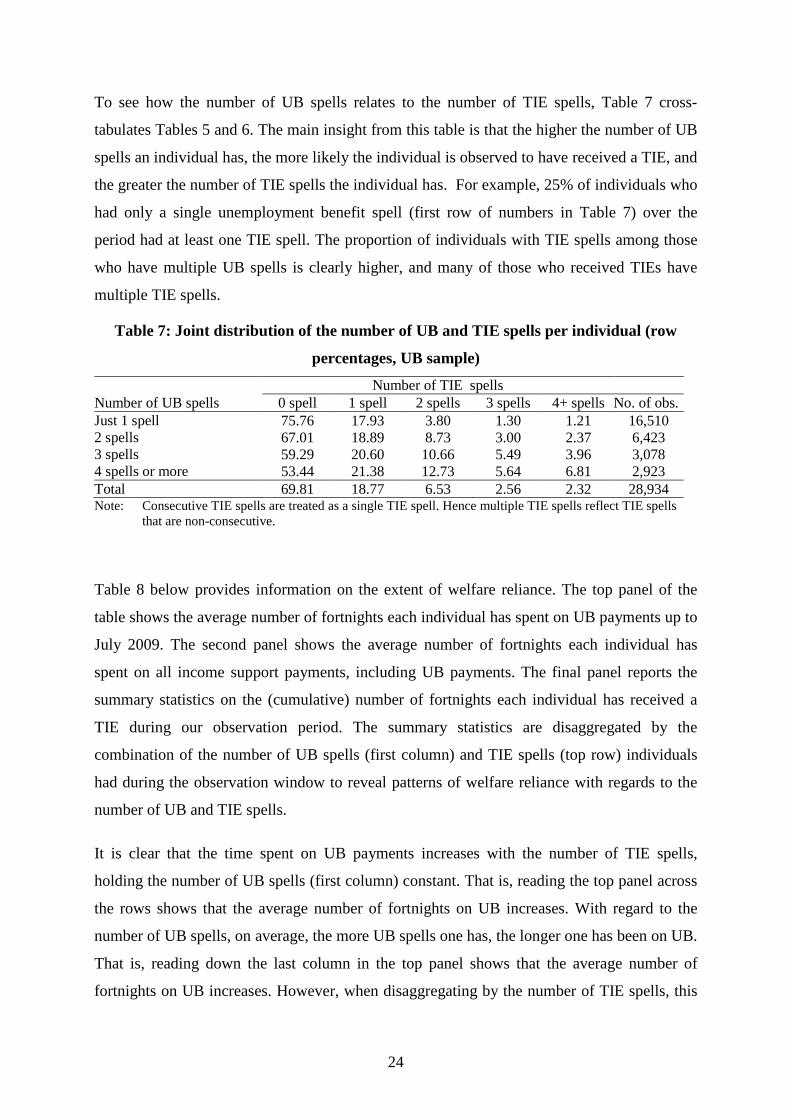
To see how the number of UB spells relates to the number of TIE spells, Table 7 cross-
tabulates Tables 5 and 6. The main insight from this table is that the higher the number of UB
spells an individual has, the more likely the individual is observed to have received a TIE, and
the greater the number of TIE spells the individual has. For example, 25% of individuals who
had only a single unemployment benefit spell (first row of numbers in Table 7) over the
period had at least one TIE spell. The proportion of individuals with TIE spells among those
who have multiple UB spells is clearly higher, and many of those who received TIEs have
multiple TIE spells.
Table 7: Joint distribution of the number of UB and TIE spells per individual (row
percentages, UB sample)
Number of TIE spells Number of UB spells 0 spell 1 spell 2 spells 3 spells 4+ spells No. of obs. Just 1 spell 75.76 17.93 3.80 1.30 1.21 16,510 2 spells 67.01 18.89 8.73 3.00 2.37 6,423 3 spells 59.29 20.60 10.66 5.49 3.96 3,078 4 spells or more 53.44 21.38 12.73 5.64 6.81 2,923 Total 69.81 18.77 6.53 2.56 2.32 28,934 Note: Consecutive TIE spells are treated as a single TIE spell. Hence multiple TIE spells reflect TIE spells
that are non-consecutive.
Table 8 below provides information on the extent of welfare reliance. The top panel of the
table shows the average number of fortnights each individual has spent on UB payments up to
July 2009. The second panel shows the average number of fortnights each individual has
spent on all income support payments, including UB payments. The final panel reports the
summary statistics on the (cumulative) number of fortnights each individual has received a
TIE during our observation period. The summary statistics are disaggregated by the
combination of the number of UB spells (first column) and TIE spells (top row) individuals
had during the observation window to reveal patterns of welfare reliance with regards to the
number of UB and TIE spells.
It is clear that the time spent on UB payments increases with the number of TIE spells,
holding the number of UB spells (first column) constant. That is, reading the top panel across
the rows shows that the average number of fortnights on UB increases. With regard to the
number of UB spells, on average, the more UB spells one has, the longer one has been on UB.
That is, reading down the last column in the top panel shows that the average number of
fortnights on UB increases. However, when disaggregating by the number of TIE spells, this

25
positive correlation only holds for those who have at most one TIE spell. In particular, the
groups that have 2 or 3 TIE spells do not show any clear patterns, while the pattern is actually
reversed for the group that have 4 or more TIE spells. That is, for the group with 4 or more
TIE spells (second last column, top panel) more UB spells is associated with less total
fortnights on UB. The average time on all income support payments (including UB) (the
second panel) reveals similar patterns as the results above. Very similar patterns are also
found for the case of the total number of fortnights with a TIE, which are reported in the third
(and last) panel of the table.

26
Table 8: The extent of welfare reliance, and time with a TIE by the number of UB and
TIE spells an individual experienced between 2002 and 2009 (UB sample)
Number of TIE spells*
Number of UB spells 0 spell 1 spell 2 spells 3 spells 4+ spells All Total of time (fortnights) on UB payments(a)
Just 1 spell mean 38.8 66.0 127.4 172.1 222.5 51.0 std. err. (61.7) (82.0) (102.5) (111.7) (102.5) (75.5) no. of obs. 12508 2960 628 215 199 16510 2 spells mean 60.8 86.4 111.9 139.1 210.1 76.0 std. err. (69.9) (84.0) (89.1) (84.6) (105.6) (81.3) no. of obs. 4304 1213 561 193 152 6423 3 spells mean 83.0 107.3 116.1 135.1 193.3 98.8 std. err. (78.4) (86.7) (78.9) (81.7) (91.4) (84.7) no. of obs. 1825 634 328 169 122 3078 4 spells or more mean 106.2 133.3 131.8 159.0 172.5 122.8 std. err. (73.9) (80.2) (82.1) (76.7) (80.2) (79.6) no. of obs. 1562 625 372 165 199 2923 All mean 52.7 83.1 121.7 152.2 199.6 68.9 std. err. (69.4) (85.9) (91.2) (92.2) (97.1) (81.9) no. of obs. 20199 5432 1889 742 672 28934 Total of time (fortnights) on all IS payments(b)
Just 1 spell mean 80.0 152.1 220.8 266.6 301.1 103.4 std. err. (113.2) (141.0) (141.5) (139.3) (134.3) (129.2) 2 spells mean 94.2 139.4 175.7 218.1 267.1 117.6 std. err. (105.7) (121.2) (124.2) (126.3) (123.6) 118.4 3 spells mean 110.2 143.2 162.0 187.7 248.6 132.2 std. err. (103.9) (111.5) (106.7) (112.9) (119.8) (112.0) 4 spells or more mean 126.0 162.2 165.3 202.7 214.2 149.1 std. err. (90.1) (98.7) (107.6) (99.6) (106.2) (100.1) All mean 89.3 149.4 186.2 221.8 258.1 114.2 std. err. (110.1) (129.3) (126.8) (125.5) (125.8) (123.3) Total of time (fortnights) on TIE (c)
Just 1 spell mean - 10.0 21.3 29.0 42.7 14.4 std. err. - (11.7) (19.4) (21.0) (27.5) (17.2) 2 spells mean - 7.2 17.0 26.0 32.8 13.3 std. err. - (7.8) (14.3) (19.2) (20.3) (14.8) 3 spells mean - 6.2 14.8 24.9 33.7 13.7 std. err. - (6.8) (12.7) (16.0) (21.8) (15.2) 4 spells or more mean - 5.4 11.5 19.4 30.5 12.4 std. err. - (5.2) (7.7) (10.7) (17.5) (12.8) All mean - 8.4 17.0 25.2 35.2 13.7 std. err. - (10.0) (15.4) (17.8) (22.7) (15.7) Note: (a) Total of fortnights on UB payments observed in the RED data up to July 2009.
(b) Total of fortnights on IS payments observed in the RED data up to July 2009. (c) Total of fortnights on TIE during July 2002- July 2009. (*) Consecutive TIE spells are treated as a single TIE spell. Hence multiple TIE spells reflect TIE spells that are non-consecutive.

27
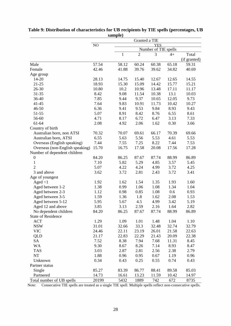
Table 9 below provides a comparison of means for two groups: UB recipients with (very last
column) and without a TIE (very first column). In addition, it also reveals how the
characteristics of UB customers who have received an exemption differ, depending on the
number of exemptions that they have received in total during the observation window. That is,
the very last column of Table 9 is split by the number of TIE spells. The unit of observation in
Table 9 is the individual and the numbers are percentages. To give an example, amongst those
UB recipients not granted a TIE, 57.54% is male (top left number). Amongst those UB
recipients granted four TIEs, 65.18% was male (same row). The personal characteristics for
individuals who had been granted TIEs are taken at the starting fortnight of the first TIE
granted to them, whereas for individuals who had never been granted a TIE the personal
characteristics relate to the starting fortnight of their first UB spell.
There are no major differences between individual characteristics across the columns, except
for gender, age and partner status. A higher proportion of males have had multiple TIE spells,
relative to women. Furthermore, the age distribution for UB recipients without TIEs is
overrepresented by individuals 25 years of age or younger when compared to the age
distribution for UB recipients with at least one TIE (i.e. last column); the age group 26 to 30
years seems to be the tipping point. In broad terms (comparing first and last columns) there
are no differences between the proportion of UB recipients with partners for those with or
without TIEs, but among those with multiple TIE spells singles are overrepresented.
Table 9b is the equivalent of Table 9 using the ATPP sample and provides a comparison of
means for activity tested PP recipients with (very last column) and without a TIE (very first
column). We find that those with a TIE, compared to those without a TIE, are more likely to
be in the age group 46 to 64 years old and less likely to be in the age group 25 to 25 years old.
Furthermore they are also more likely to have been born overseas in a non-English-speaking
country and more likely to have only one dependent child. Their youngest child is also more
likely to be more than 12 years of age.
28
Table 9: Distribution of characteristics for UB recipients by TIE spells (percentages, UB sample)
Granted a TIE NO YES Number of TIE spells 1 2 3 4+ Total
(if granted) Male 57.54 58.12 60.24 60.38 65.18 59.31 Female 42.46 41.88 39.76 39.62 34.82 40.69 Age group
14-20 28.13 14.75 15.40 12.67 12.65 14.55 21-25 18.93 15.30 15.09 14.42 15.77 15.21 26-30 10.80 10.2 10.96 13.48 17.11 11.17 31-35 8.42 9.08 11.54 10.38 13.1 10.03 36-40 7.85 9.44 9.37 10.65 12.05 9.73 41-45 7.64 9.83 10.91 11.73 10.42 10.27 46-50 6.36 9.41 9.53 9.84 8.93 9.43 51-55 5.07 8.91 8.42 8.76 6.55 8.61 56-60 4.71 8.17 6.72 6.47 3.13 7.33 61-64 2.08 4.92 2.06 1.62 0.30 3.66
Country of birth Australian born, non ATSI 70.32 70.07 69.61 66.17 70.39 69.66 Australian born, ATSI 6.55 5.63 5.56 5.53 4.61 5.53 Overseas (English speaking) 7.44 7.55 7.25 8.22 7.44 7.53 Overseas (non-English speaking) 15.70 16.75 17.58 20.08 17.56 17.28
Number of dependent children 0 84.20 86.25 87.67 87.74 88.99 86.89 1 7.10 5.82 5.29 4.85 3.57 5.45 2 5.07 4.22 4.24 4.99 3.72 4.25 3 and above 3.62 3.72 2.81 2.43 3.72 3.41
Age of youngest Aged <1 1.92 1.62 1.54 1.35 1.93 1.60 Aged between 1-2 1.38 0.99 1.06 1.08 1.34 1.04 Aged between 2-3 1.12 0.98 0.85 1.08 0.6 0.93 Aged between 3-5 1.59 1.36 1.8 1.62 2.08 1.53 Aged between 5-12 5.95 5.67 4.5 4.99 3.42 5.19 Aged 12 and above 3.85 3.13 2.59 2.16 1.64 2.82 No dependent children 84.20 86.25 87.67 87.74 88.99 86.89
State of Residence ACT 1.29 1.09 1.01 1.48 1.04 1.10 NSW 31.01 32.66 33.3 32.48 32.74 32.79 VIC 24.46 22.11 23.19 26.01 21.58 22.63 QLD 21.17 22.83 22.29 21.43 20.09 22.38 SA 7.52 8.38 7.94 7.68 11.31 8.45 WA 9.30 8.67 8.26 7.14 8.93 8.47 TAS 3.03 2.87 2.81 2.56 2.38 2.79 NT 1.88 0.96 0.95 0.67 1.19 0.96 Unknown 0.34 0.43 0.25 0.55 0.74 0.43
Partner status Single 85.27 83.39 86.77 88.41 89.58 85.03 Partnered 14.73 16.61 13.23 11.59 10.42 14.97
Total number of UB spells 20199 5432 1889 742 672 8735 Note: Consecutive TIE spells are treated as a single TIE spell. Multiple spells reflect non-consecutive spells.

29
Table 9b: Distribution of characteristics for activity tested PP recipients by TIE spells (percentages, ATPP sample)
Granted a TIE NO YES Number of TIE spells 1 2 3+ Total
(if granted) Male 9.16 8.96 7.81 7.69 8.67 Female 90.84 91.04 92.19 92.31 91.33 Age group
14-20 0.07 0.03 0.00 0.00 0.02 21-35 32.02 24.54 24.28 24.91 24.51 36-45 49.37 49.38 48.02 54.95 49.43 46-64 18.54 26.05 27.70 20.15 26.03
Country of birth Australian born, non ATSI 66.88 64.06 64.71 62.64 64.10 Australian born, ATSI 6.44 5.71 5.78 3.66 5.61 Overseas (English speaking) 7.97 7.75 7.06 7.33 7.60 Overseas (non-English speaking) 18.71 22.48 22.46 26.37 22.69
Number of dependent children 1 48.07 55.72 53.37 56.78 55.34 2 34.53 31.61 32.83 32.60 31.90 3 and above 17.40 12.67 13.80 10.62 12.76
Age of youngest Aged between 6-12 73.51 64.48 65.24 61.90 64.49 Aged 12 and above 26.49 35.62 34.76 38.10 35.51
State of Residence ACT 1.05 1.21 1.39 2.20 1.30 NSW 32.53 33.26 33.69 35.16 33.45 VIC 24.1 24.54 26.52 22.34 24.8 QLD 20.26 19.8 21.07 18.68 19.98 SA 7.92 9.58 8.02 11.72 9.4 WA 9.58 7.97 5.88 6.96 7.52 TAS 2.95 2.92 3.1 1.47 2.88 NT 1.55 0.67 0.21 1.10 0.61 Unknown 0.06 0.05 0.11 0.37 0.08
Partner status Single 86.40 88.06 87.38 89.38 88.01 Partnered 13.60 11.94 12.62 10.62 11.99
Total number of ATPP spells 27,226 3,728 935 273 4,936 Note: Consecutive TIE spells are treated as a single TIE spell. Multiple spells reflect non-consecutive spells.
4.4. Transitions in Income Support Receipt for Individuals granted TIEs
To assess how UB recipients who have been granted TIEs fare we follow them over time.
Specifically, we select UB spells commenced within our observation window that last longer
than 6 months and measure the number of TIE spells and the total of TIE fortnights within the
initial 6 months of these UB spells. Next, we follow those recipients up at 6 months, 12
months, and then every year up to 4 years from the end of the initial 6 month period (on UB).

30
At each follow-up point we check to see if they are still on UB, have transited to DSP, have
transited to an income support payment other than DSP, or have left income support
altogether. Table 10 reports our analysis statistics of this follow-up group. Also, because some
TIE spells occur much later into the UB spell (as observed in Table 3), we repeat the follow-
up analysis but condition on individuals who start an UB spell that lasts longer than 12
months and measure the number of TIE spells and the total of TIE fortnights they have within
the first 12 months of their UB spell. The statistics for this group are reported in Table 11.
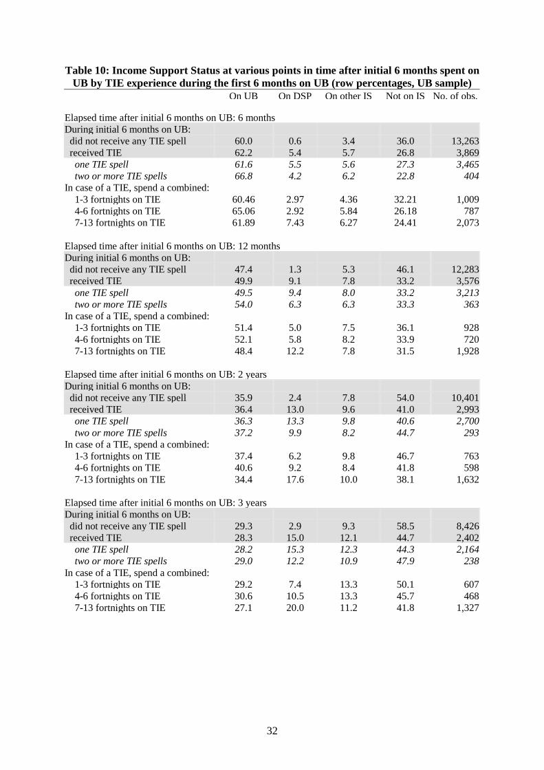
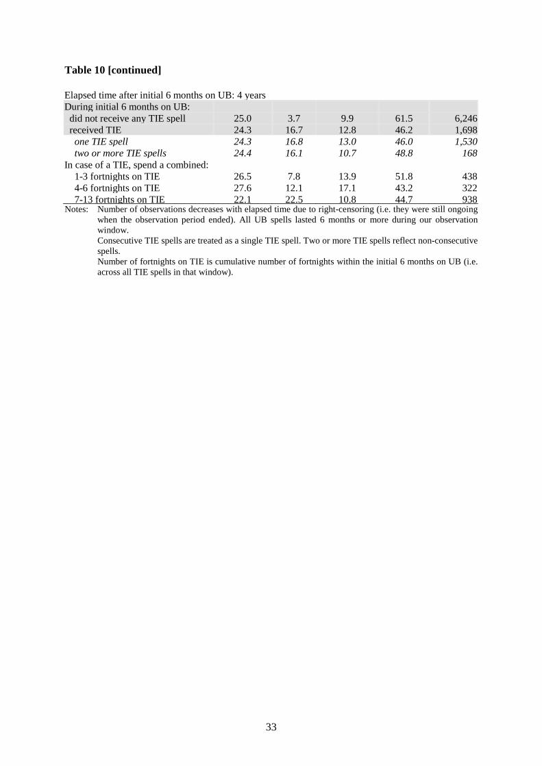
Table 10 shows that the proportion of individuals that has left income support 6 months after
the end of the first 6 months on UB differs by TIE receipt status. For those who did not
receive a TIE this proportion is 36%. For those who received TIEs, it is about a quarter. As
for subsequent follow-up points, the rate of leaving income support still differs by whether or
not an individual has ever been granted TIEs to the same extent as it did at the 6 month
follow-up point. In addition, the rate of leaving income support also differs within the group
of customers that received TIEs, although differences by the number of TIE spells and the
total number of fortnights with a TIE are both small. The proportion leaving income support
is negatively correlated with the total number of fortnights with a TIE.
As for the outcome of being on UB, the proportion does not differ substantially between TIE
receipt statuses. However, when disaggregating by the number of TIE spells, recipients with
multiple TIE spells are more likely to stay on UB, compared to those with one single spell, for
the follow-up points of 6 months and 12 months. This pattern, however, does not hold for the
subsequent follow-up points.
There are substantial differences in the proportions transferring to DSP and other payments
with respect to TIE receipt status. Individuals who received TIEs are much more likely to
transfer to DSP compared to those who did not. By the end of year 4 (after the initial 6
months), 16% of individuals with TIEs are found to be receiving DSP, compared to 3.7%
among those who did not have a TIE. The rate of transferring to DSP also differs among those
with TIEs. Individuals who received TIE for a longer duration are much more likely to
transfer to DSP, when compared to those who had short TIE spells, and this pattern holds for
every follow-up point. On the contrary, recipients with multiple TIE spells are less likely to
transfer to DSP, compared to those with a single TIE spell and this pattern is true for every
follow-up point. Similar conclusions are also found for the outcome of transferring to other
payments, but to a lesser extent.

31
Overall, the key patterns with respect to the receipt of TIE are as follows. Those who had no
TIE spell are more likely to leave the income support system whereas those who had a TIE
spell are more likely to transfer to DSP and other income support payments. Furthermore, the
probability of transferring to DSP is positively related to the amount of time customers
received a TIE.
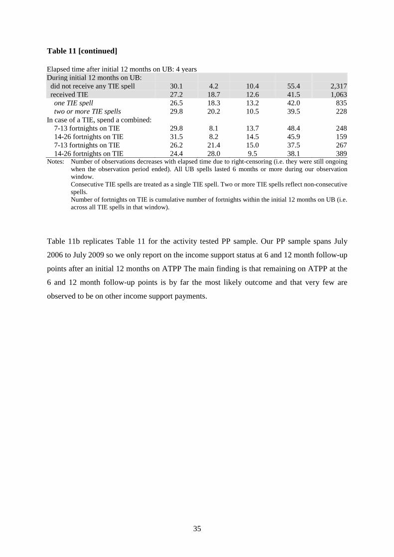
The results in Table 11 replicates those in Table 10 for the case where we condition on
individuals who start an UB spell that lasts at least 12 months and where we measure the
number of TIE spells and the number of TIE fortnights within their first 12 months on UB. In
other words, we have changed our population- we now capture those individuals who have
very long episodes of continuous unemployment (by construction, at least 12 months). This is
reflected, for instance, in the proportion of those who were still on UB at the first follow-up 6
months later - around 70% is still on UB as opposed to the 60% in Table 10.
With respect to the differences in terms of TIE experiences, the patterns are quite similar to
those shown in Table 10. For example, as the length between follow-ups increases more
individuals move off income support or transfer to other payments. Similarly, for those who
had TIEs, a common transition is to DSP and the rate of transition increases with the number
of fortnights with a TIE. With respect to transfers to income support payments (other than
DSP), the patterns do not seem to differ substantially by whether or not an individual was
granted a TIE or not. However, there is a different pattern between Tables 10 and 11. While
Table 10 shows there is a difference in the outcomes at various follow-up points by the
number of TIE spells, the outcomes at various follow-up points for recipients with multiple
TIE spells and single TIE spells in Table 11 are quite similar to each other.
32
Table 10: Income Support Status at various points in time after initial 6 months spent on UB by TIE experience during the first 6 months on UB (row percentages, UB sample)
On UB On DSP On other IS Not on IS No. of obs. Elapsed time after initial 6 months on UB: 6 months During initial 6 months on UB: did not receive any TIE spell 60.0 0.6 3.4 36.0 13,263 received TIE 62.2 5.4 5.7 26.8 3,869 one TIE spell 61.6 5.5 5.6 27.3 3,465 two or more TIE spells 66.8 4.2 6.2 22.8 404 In case of a TIE, spend a combined: 1-3 fortnights on TIE 60.46 2.97 4.36 32.21 1,009 4-6 fortnights on TIE 65.06 2.92 5.84 26.18 787 7-13 fortnights on TIE 61.89 7.43 6.27 24.41 2,073 Elapsed time after initial 6 months on UB: 12 months During initial 6 months on UB: did not receive any TIE spell 47.4 1.3 5.3 46.1 12,283 received TIE 49.9 9.1 7.8 33.2 3,576 one TIE spell 49.5 9.4 8.0 33.2 3,213 two or more TIE spells 54.0 6.3 6.3 33.3 363 In case of a TIE, spend a combined: 1-3 fortnights on TIE 51.4 5.0 7.5 36.1 928 4-6 fortnights on TIE 52.1 5.8 8.2 33.9 720 7-13 fortnights on TIE 48.4 12.2 7.8 31.5 1,928 Elapsed time after initial 6 months on UB: 2 years During initial 6 months on UB: did not receive any TIE spell 35.9 2.4 7.8 54.0 10,401 received TIE 36.4 13.0 9.6 41.0 2,993 one TIE spell 36.3 13.3 9.8 40.6 2,700 two or more TIE spells 37.2 9.9 8.2 44.7 293 In case of a TIE, spend a combined: 1-3 fortnights on TIE 37.4 6.2 9.8 46.7 763 4-6 fortnights on TIE 40.6 9.2 8.4 41.8 598 7-13 fortnights on TIE 34.4 17.6 10.0 38.1 1,632 Elapsed time after initial 6 months on UB: 3 years During initial 6 months on UB: did not receive any TIE spell 29.3 2.9 9.3 58.5 8,426 received TIE 28.3 15.0 12.1 44.7 2,402 one TIE spell 28.2 15.3 12.3 44.3 2,164 two or more TIE spells 29.0 12.2 10.9 47.9 238 In case of a TIE, spend a combined: 1-3 fortnights on TIE 29.2 7.4 13.3 50.1 607 4-6 fortnights on TIE 30.6 10.5 13.3 45.7 468 7-13 fortnights on TIE 27.1 20.0 11.2 41.8 1,327
33
Table 10 [continued] Elapsed time after initial 6 months on UB: 4 years During initial 6 months on UB: did not receive any TIE spell 25.0 3.7 9.9 61.5 6,246 received TIE 24.3 16.7 12.8 46.2 1,698 one TIE spell 24.3 16.8 13.0 46.0 1,530 two or more TIE spells 24.4 16.1 10.7 48.8 168 In case of a TIE, spend a combined: 1-3 fortnights on TIE 26.5 7.8 13.9 51.8 438 4-6 fortnights on TIE 27.6 12.1 17.1 43.2 322 7-13 fortnights on TIE 22.1 22.5 10.8 44.7 938 Notes: Number of observations decreases with elapsed time due to right-censoring (i.e. they were still ongoing
when the observation period ended). All UB spells lasted 6 months or more during our observation window. Consecutive TIE spells are treated as a single TIE spell. Two or more TIE spells reflect non-consecutive spells. Number of fortnights on TIE is cumulative number of fortnights within the initial 6 months on UB (i.e. across all TIE spells in that window).

34
Table 11: Income Support Status at various points in time after initial 12 months spent on UB by TIE experience during first 12 months on UB (row percentages, UB sample)
On UB On DSP On other IS Not on IS No. of obs. Elapsed time after initial 12 months on UB: 6 months During initial 12 months on UB: did not receive any TIE spell 70.0 0.9 2.8 26.3 5,601 received TIE 71.8 5.1 4.8 18.3 2,694 one TIE spell 71.3 5.2 4.8 18.7 2,055 two or more TIE spells 73.4 5.0 4.5 17.1 639 In case of a TIE, spend a combined: 1-3 fortnights on TIE 71.4 2.5 3.5 22.6 601 4-6 fortnights on TIE 72.1 2.4 4.4 21.2 458 7-13 fortnights on TIE 72.8 3.8 6.7 16.7 731 14-26 fortnights on TIE 71.1 9.3 4.2 15.4 904 Elapsed time after initial 12 months on UB: 12 months During initial 12 months on UB: did not receive any TIE spell 57.1 1.9 4.8 36.3 5,145 received TIE 57.2 8.3 6.6 27.9 2,472 one TIE spell 56.8 7.9 6.9 28.4 1,890 two or more TIE spells 58.4 9.5 5.7 26.5 582 In case of a TIE, spend a combined: 7-13 fortnights on TIE 57.8 3.5 5.5 33.3 547 14-26 fortnights on TIE 59.2 3.9 7.7 29.2 414 7-13 fortnights on TIE 57.9 7.6 8.3 26.3 662 14-26 fortnights on TIE 55.2 14.1 5.5 25.1 849 Elapsed time after initial12 months on UB: 2 years During initial 12 months on UB: did not receive any TIE spell 43.2 2.9 7.7 46.2 4,253 received TIE 42.2 13.6 9.1 35.1 2,043 one TIE spell 42.8 12.8 9.0 35.4 1,557 two or more TIE spells 40.3 16.1 9.5 34.2 486 In case of a TIE, spend a combined: 7-13 fortnights on TIE 45.1 5.1 8.5 41.3 448 14-26 fortnights on TIE 44.9 5.4 8.4 41.3 332 7-13 fortnights on TIE 45.4 13.4 10.4 30.7 537 14-26 fortnights on TIE 36.9 22.6 8.8 31.7 726 Elapsed time after initial 12 months on UB: 3 years During initial 12 months on UB: did not receive any TIE spell 35.3 3.8 8.9 52.0 3,288 received TIE 33.0 16.4 11.7 38.9 1,559 one TIE spell 33.3 15.6 11.9 39.3 1,187 two or more TIE spells 32.3 18.8 11.3 37.6 372 In case of a TIE, spend a combined: 7-13 fortnights on TIE 39.9 5.0 11.7 43.4 341 14-26 fortnights on TIE 37.0 5.6 11.7 45.8 249 7-13 fortnights on TIE 32.9 17.6 13.9 35.6 404 14-26 fortnights on TIE 27.3 27.1 10.3 35.4 565
35
Table 11 [continued] Elapsed time after initial 12 months on UB: 4 years During initial 12 months on UB: did not receive any TIE spell 30.1 4.2 10.4 55.4 2,317 received TIE 27.2 18.7 12.6 41.5 1,063 one TIE spell 26.5 18.3 13.2 42.0 835 two or more TIE spells 29.8 20.2 10.5 39.5 228 In case of a TIE, spend a combined: 7-13 fortnights on TIE 29.8 8.1 13.7 48.4 248 14-26 fortnights on TIE 31.5 8.2 14.5 45.9 159 7-13 fortnights on TIE 26.2 21.4 15.0 37.5 267 14-26 fortnights on TIE 24.4 28.0 9.5 38.1 389 Notes: Number of observations decreases with elapsed time due to right-censoring (i.e. they were still ongoing
when the observation period ended). All UB spells lasted 6 months or more during our observation window. Consecutive TIE spells are treated as a single TIE spell. Two or more TIE spells reflect non-consecutive spells. Number of fortnights on TIE is cumulative number of fortnights within the initial 12 months on UB (i.e. across all TIE spells in that window).
Table 11b replicates Table 11 for the activity tested PP sample. Our PP sample spans July
2006 to July 2009 so we only report on the income support status at 6 and 12 month follow-up
points after an initial 12 months on ATPP The main finding is that remaining on ATPP at the
6 and 12 month follow-up points is by far the most likely outcome and that very few are
observed to be on other income support payments.

36
Table 11b: Income Support Status at various points in time after initial 12 months spent on ATPP by TIE experience during the first 12 months on ATPP (row percentages)
On ATPP On other IS Not on IS No. of obs. Elapsed time after initial 12 months on ATPP: 6 months During initial 6 months on ATPP: did not receive any TIE spell 84.4 1.4 14.1 15735 received TIE 81.6 2.4 16.1 2364 In case of a TIE, spend a combined: 1-3 fortnights on TIE 83.3 2.3 14.4 750 4-6 fortnights on TIE 82.9 1.9 15.1 463 7-13 fortnights on TIE 79.8 2.4 17.7 739 14-26 fortnights on TIE 79.9 2.9 17.2 412 Elapsed time after initial 12 months on ATPP: 12 months During initial 6 months on ATPP: did not receive any TIE spell 73.5 0.7 25.8 14332 received TIE 68.4 0.9 30.7 2299 In case of a TIE, spend a combined: 7-13 fortnights on TIE 69.4 1.0 29.6 731 14-26 fortnights on TIE 70.6 0.9 28.5 449 7-13 fortnights on TIE 67.0 0.3 32.7 716 14-26 fortnights on TIE 66.8 1.4 31.8 403 Notes: Number of observations decreases with elapsed time because of right censoring (i.e. they were still
ongoing when the observation period ended). All ATPP spells lasted 12 months or more during our observation window. Number of fortnights on TIE is cumulative number of fortnights within the initial 6 or 12 months on ATPP (i.e. across all TIE spells in that window).

37
5. Modelling approach
In this section, we aim to examine the impact of receiving TIEs on the individual’s future use
of income support payments. In particular, we want to investigate whether the use of TIEs is
associated with a higher chance of moving to non-activity tested payments, especially DSP.
So far, from the descriptive analysis, we learned that for the UB sample
• Individuals with TIEs on average spend more time on income support payments
• Individuals with TIEs also spend a longer time on unemployment benefits, in
other words, many of those individuals are long-term unemployed.
• Individuals with TIEs tend to be older compared to individuals without TIEs.
Compared to descriptive analysis, models have the advantage that a multitude of factors can
be incorporated simultaneously. To do the same with descriptive analysis is much less
straight-forward. For example, descriptive analysis on the relationship between age and the
use of TIEs and, say, country of birth and the use of TIEs could be expanded by using cross
tabulations of age and country of birth if there is a concern that most migrants are
overrepresented among certain age groups. In the descriptive analysis in the previous section
we often used cross tabulations of the number of UB and TIE spells. However, when the
number of characteristics becomes larger these cross tabulations become impractical due to
the number of possible combinations. This is where models are useful. We will briefly
describe our modelling approach, which is used to estimate two models. Model 1 corresponds
to the second block of numbers in Table 10. Model 2 corresponds to the second block of
numbers in Table 11. We also estimate a variation of model 2 for the PP sample.
There are several important points about our estimation approach. First, by including
demographic and income support history, we are able to control in part for differences
between the groups of individuals with TIEs and the group of individuals without TIEs.
Second, by restricting the sample to UB spells that lasted a certain period and derived the
TIE-related variables for that period, we attempt to reduce the differences between the two
groups of individuals. The model results should really be interpreted as an alternative
representation of a multi-dimensional cross tabulation. That is, our objective is to establish
correlations and general patterns, not strictly causal relationships.

38
Model 1
For the first estimation, we restrict the UB spells commenced within the data period to have
lasted at least 6 months. We derive variables that capture the use of TIEs within the initial 6
months of the UB spells. Our dependent variable is the status of income support receipt at 12
months after the initial 6 months on UB (i.e. 18 months since the UB spell commencement).
We distinguish four outcomes for the dependent variable: (Still or again) on UB, on DSP, on
other payments, and off income support.
We model these four potential outcomes using a multinomial logit model. To measure the
impact of the use of TIEs within the initial 6 months of the UB spell on the outcome
variables, we include:
o The use of TIEs
o Did not received any TIE (omitted category)
o Received one TIE spell
o Received two or more TIE spells
o Time spent on TIEs within the initial 6 months UB spell (in fortnights).
In addition to these TIE related variables, we also control for the following factors
o Age
o Aged 20 years and under (omitted category)
o Aged 21-25 years
o Aged 26-30 years
o Aged 31-35 years
o Aged 36-40 years
o Aged 41-45 years
o Aged 46-50 years
o Aged 51-55 years
o Aged 56+ years
o Gender (male is omitted category)
o Country of birth and ATSI status
o Non ATSI Australian born (omitted category)
o ATSI
39
o ESB ( foreign born; born in a major English speaking country)
o NESB (foreign born; born in a non-English speaking country)
o Partner status (at spell entry)
o Presence of dependent child(ren) (at spell entry)
o Region of residence (at spell entry)
o Sydney (omitted category)
o Balance of New South Wales (NSW)
o Brisbane
o Balance of Queensland (QLD)
o Adelaide
o Balance of South Australia (SA)
o Perth
o Balance of Western Australia (WA)
o Tasmania (TAS)
o Northern Territory, Australian Capital Territory (NT/ACT)
o Year of spell entry
o 2002 (omitted category)
o 2003
o 2004
o 2005
o 2006
o 2007
o 2008
o Income support history in the 2 years prior to the start of the (minimum 6 month) UB
spell
o Indicator for receiving UB
o Indicator for receiving other income support payments
Model 2
Model 2 is identical in set up to Model 1 except that, instead of restricting the UB spells
commenced within the data period to have lasted at least 6 months we now restrict them to
have lasted at least 12 months. We derive the same variables that capture the use of TIEs
within the initial 12 months of the UB spell. The dependent variable is again the status of

40
income support receipt at the 12-month follow-up (i.e. 2 years since the UB spell
commencement).
Samples for Models 1 and 2 correspond to the second block of numbers in Table 10 and Table
11, respectively. It is important to point out that both samples have excluded short-term
unemployment spells that lasted less than 6 months, which make up the bulk of all spells. The
sample for the latter model excludes individuals who left UB from month 7 to month 12 since
spell commencement and hence is smaller than the sample used in model 1. However, the
smaller sample for model 2 does have the advantage of observing more TIEs, since TIEs are
often granted later on into an UB spell (see Table 3).
Before presenting and discussing the estimation results, we first describe our econometric
model – the multinomial logit model.
5.1. The multinomial logit model
We present the multinomial logit model, using the first estimation as the illustration. The
probability an UB recipient is in outcome state j 18 months after commencement of the UB
spell is modelled as a function of the individual’s characteristics and other factors denoted by
X, i.e.,
( , )j jP P X β=
where jβ is a vector of parameters. The multinomial logit model is defined by letting P(.) take
a logit probability function. It is identified by normalising the parameters β to zero for one
outcome (the base category) and is described by the system of equations:
( )
( )
2
2
1Pr 11
Pr , 2,...,1
j
m
j
J
j
J
j
ye
ey m m Je
=
=
= =+
= = =+
∑
∑
Xβ
Xβ
Xβ
where X is a vector of explanatory variables, βj is the coefficient vector for outcome J and y is
the outcome of interest that can take on J distinct values. In our case y can take on the value 1
(being on UB), 2 (being on DSP), 3 (being on income support, but not UB or DSP), and 4

41
(being off income support). We normalise the β1 to be zero, that is, we take being on UB as
the reference outcome. What one chooses as the reference outcome is completely
inconsequential. It only affects for which outcomes estimated coefficients are presented. The
coefficient estimates are not intuitively interpretable in any event, as the model is non-linear
and the effects of individual explanatory variables depend on the values of the explanatory
variables at which they are evaluated. Consequently, rather than focussing on coefficient
estimates, ‘mean marginal effects’ of the explanatory variables are reported and analysed.
These marginal effects are available for all the outcomes of the dependent variable and do not
require a normalisation as is the case for the βs.
The marginal effect of continuous explanatory variable xk on the probability that outcome m
occurs for a person with characteristics ix is given by:
( ) ( ) ( ), , | , |
1
Pr |Pr | Pr |
i Ji i im k k m J k j Ji
j
y mME y m y j
xβ β
=
∂ = = = = − = ∂
∑x
x x
while the mean marginal effect is given by:
( ), ,1
1/n
im k m k
iMME n ME
=
= ∑
where ,m kMME is the mean marginal effect of variable kx on the predicted probability
( )Pr |y m x= , and the summation is over the n individuals in the sample. This is, as the name
suggests, the mean marginal effect of the explanatory variable on the predicted probability a
person has outcome m, is evaluated over all individuals in the sample, and holding all other
explanatory variables constant at their actual values. To put the maths in plain language, the
mean marginal effect is ‘the average effect on the probability of outcome m per unit of
increase in kx ’.
For a binary explanatory variable, the marginal effect of explanatory variable kx on the
probability outcome m occurs for a person with characteristics ix is given by:
( ) ( ), Pr | , 1 Pr | , 0i i im k k k k kME y m x y m x− −= = = − = =x x
42
where ik−x represents the vector of characteristics of person i for all variables other than kx .
That is, the marginal effect is obtained by changing the explanatory variable kx from zero to
one. When doing this for every individual, holding all other explanatory variables at their
actual values, and calculating the mean change in the predicted probability one obtains the
mean marginal effect for kx .
For related sets of binary variables, such as those for age groups, we also take account of the
dependencies between these variables in calculating mean marginal effects. Specifically, we
first set all of the interdependent dummy variables equal to zero before calculating the effect
of changing the specific dummy variable from zero to one for each individual. For example,
to calculate the mean marginal effect for the ‘age 36-40’ dummy, we first set all age dummies
to zero for each individual before setting the ‘age 36-40’ dummy to 1, thereby giving us the
effect of changing a person’s age from “ 20 or less” (the omitted dummy) to 36-40.
The correspondingly modified version of the marginal effect (ME) equation is therefore:
( ) ( ), Pr | , 0, 1 Pr | , 0, 0i i im k o g k o g kME y m x y m x= = = = − = = =x x x x
where iox comprises a vector of characteristics of person i for all variables other than those in
the group of dummy variables to which variable kx belongs, and gx is the vector of other
dummy variables in the group to which kx belongs.
Note that the mean marginal effect of a variable sums to zero across the J possible outcome
categories, i.e. ,1
0J
j kj
MME=
=∑ . The logic behind this is simple. If a characteristic ‘x’ makes
someone more likely to have exited income support, then it must make them less likely to be
in any of the remaining outcomes, since they have to be, and can only be, in one of the 4
outcomes.
Rather than attempt to derive analytic standard errors, standard errors for the estimates of
mean marginal effects are derived using bootstrapping. The standard error of any statistic M
can be computed as:
2
1 1
1 1ˆ ˆ1
B Bi i
Mi i
SE M MB B= =
= − − ∑ ∑
43
where B is the number of bootstrap iterations (we choose 400 iterations) and ˆ iM is the value
of M in the ith bootstrap sample. Of course, one can also simply refer to the significance level
of the raw coefficient estimates to see which variables are statistically significant.
5.2. Estimation Results
Tables 12 and 13 report the mean marginal effects for Models 1 and 2, respectively, for the
UB sample. The estimated coefficients, which do not have straightforward interpretation, are
reported in the Appendix (Tables A1 and A2) and not discussed here. We instead focus on the
mean marginal effects, which have a more intuitive interpretation.
We are primarily interested in the role of TIEs. We include indicators for having had “one
TIE spell” and “two or more TIE spells” during the initial months of the UB spell (either 6 or
12 months). We further include the number of fortnights with a TIE in the initial 6 or 12
months of the UB spell to account for the fact that a single TIE spell can be quite long, since
consecutive renewals/extensions are treated as a single spell. As is apparent from Tables 12
and 13, having received a TIE has a substantial impact on the four outcomes. For instance,
focusing on Table 12, the impacts of “one TIE spell” and “two or more TIE spells” on the
probability of leaving income support are substantial and similar to each other. Both are
around 10 percentage points. Having received one TIE spell increases the probability of being
on UB by almost 4 percentage points and around 3 percentage points for the remaining
outcomes (on DSP and on other payment). As for the case of having received two or more
TIE spells, its negative impact of 10% on the outcome of leaving income support is mostly
translated into its positive impact on the probability of staying on UB (7.3%).
The effects of having received TIEs (by the number of spells) have been consistent with the
implied patterns reported in Table 10. With respect to the number of fortnights with a TIE, the
estimated effects are not significant- only the effect on DSP is statistically significant but
small in magnitude. This finding is in contrast with the implied pattern in Table 10. This
difference highlights that the fact that these estimated effects are conditional on a series of
control variables while the effects implied in the cross tabulations in Table 10 did not control
for any mitigating factors.
When we expand the initial UB spell period to 12 months (Table 13) the effects of having
received TIEs are still qualitatively similar. In terms of magnitude, the marginal effects of

44
time with a TIE are similar but the estimated effects of TIE receipt (by the number of TIE
spells) are smaller. Specifically, having a TIE spell reduces the probability of being off
income support by about 6 percentage points (compared to 9.4 percentage points previously)
and in the case of two or more TIE spells by about 8 percentage points (compared to 10.2
percentage points previously). It is important to keep in mind that we compare the impacts of
TIEs to the reference cases of not having any TIEs. Such reference cases for UB spells of 12
months or more are long-term unemployed individuals who already have a lower propensity
to move off income support and a higher propensity to transfer to other payments when
compared to the reference cases for UB spells of 6 months or more. The relative differences
in the impacts of TIEs between the two models highlight the possibility of the impacts of TIEs
differing across the population.
The remaining variables are primarily used as control variables and we shall briefly discuss
the main findings. Focusing on Model 1 results (Table 12), the probability of remaining on
UB is U-shaped with respect to age while the probability of transferring to DSP consistently
increases with age. The patterns in age effects for the outcomes of “on other IS” and “off IS”
are almost the mirror images of outcomes of “on UB” and “on DSP” respectively.
Female recipients are found to be much more likely to transfer to other payments but less
likely to be on UB or off income support payment compared to male recipients. Married
individuals are less likely to stay on UB and slightly more likely to transfer to DSP and much
more likely to transfer to other payments, compared to individuals without a partner. Having
dependent children, however, does not appear to have any effect.
As for the country of birth and ethnicity effects, individuals with an ATSI background are less
likely to be “Off Income Support” and more likely to “on UB” and “other IS”. Being born in a
non-English speaking country is associated with a lower (higher) probability of being off
income support (on UB).
In terms of customers’ previous experience with the income support system, having received
UB within two years prior to current spell commencement is associated with a lower (higher)
probability of being off income support (on UB). Similarly, having received other payments
increases the probabilities for the outcomes of “on UB”, “on DSP” and “other IS”, and hence
decreases the probability of being “off Income Support”.

45
Model 2 results (Table 13) are qualitatively similar to those of Model 1. In terms of
magnitude, the age effects are very similar. However, for the remaining variables, the effects
are consistently smaller in Model 2.

46
Table 12: Multinomial logit Mean Marginal Effects: Income Support Receipt Status at 12 month follow-up after initial 6 months on UB (UB sample)
On U.B On DSP On other IS Off IS M.E S.E M.E S.E M.E S.E M.E S.E TIE history within initial 6 months since entry Have one TIE spell 0.038** 0.017 0.028** 0.006 0.028** 0.008 -0.094** 0.017 Have 2+ TIE spells 0.073** 0.031 0.015* 0.008 0.014 0.015 -0.102** 0.030 No. of fortnights with TIE -0.000 0.002 0.003** 0.000 0.000 0.001 -0.003 0.002 Age at spell entry Age 21-25 -0.055** 0.012 0.002 0.003 -0.006 0.008 0.059** 0.011 Age 26-30 -0.026* 0.015 0.004 0.004 -0.020** 0.008 0.041** 0.014 Age 31-35 0.008 0.015 0.012** 0.005 -0.021** 0.008 0.001 0.015 Age 36-40 0.000 0.016 0.021** 0.005 -0.043** 0.007 0.022 0.016 Age 41-45 0.005 0.016 0.026** 0.005 -0.056** 0.007 0.025 0.015 Age 46-50 0.034** 0.017 0.030** 0.005 -0.056** 0.007 -0.008 0.017 Age 51-55 0.093** 0.019 0.045** 0.007 -0.054** 0.007 -0.084** 0.018 Age 56+ 0.077** 0.018 0.057** 0.008 0.051** 0.012 -0.185** 0.016 Female -0.035** 0.008 -0.004 0.003 0.071** 0.004 -0.032** 0.007 family status (at spell entry) Married -0.069** 0.012 0.008** 0.004 0.044** 0.006 0.016 0.013 Have dependent child 0.023 0.014 -0.005 0.004 -0.001 0.006 -0.017 0.014 ATSI and country of birth ATSI 0.105** 0.016 0.013 0.008 0.021** 0.008 -0.139** 0.015 ESB -0.019 0.017 -0.006 0.004 0.005 0.008 0.021 0.017 NESB 0.058** 0.012 0.000 0.003 0.007 0.006 -0.065** 0.011 Region of Residence (at spell entry) Balance of NSW 0.011 0.014 0.009* 0.005 -0.007 0.007 -0.013 0.014 Melbourne -0.001 0.014 0.000 0.005 -0.019** 0.006 0.019 0.014 Balance of VIC 0.058** 0.018 -0.005 0.006 -0.007 0.009 -0.046** 0.017 Brisbane -0.043** 0.017 0.003 0.006 -0.016** 0.008 0.056** 0.017 Balance of QLD -0.027* 0.015 -0.011** 0.004 -0.006 0.007 0.044** 0.014 Adelaide 0.007 0.019 0.002 0.006 -0.017* 0.009 0.008 0.018 Balance of SA 0.032 0.025 -0.008 0.007 0.010 0.013 -0.034 0.023 Perth -0.080** 0.019 0.004 0.008 -0.021** 0.008 0.097** 0.020 Balance of WA 0.010 0.024 -0.007 0.008 -0.009 0.011 0.006 0.024 TAS 0.068** 0.024 -0.013* 0.007 -0.012 0.012 -0.043* 0.023 NT/ACT 0.037 0.029 -0.011 0.008 -0.013 0.013 -0.013 0.028 Spell cohorts spells started in 2003 -0.013 0.014 0.008 0.005 -0.027** 0.007 0.031** 0.014 spells started in 2004 -0.011 0.015 0.001 0.005 -0.026** 0.007 0.036** 0.014 spells started in 2005 -0.032** 0.015 0.000 0.005 -0.029** 0.007 0.062** 0.014 spells started in 2006 -0.021 0.015 0.010** 0.005 -0.037** 0.008 0.048** 0.015 spells started in 2007 0.009 0.017 0.015** 0.005 -0.025** 0.008 0.001 0.016 spells started in 2008 0.048 0.037 0.022 0.014 -0.024 0.016 -0.046 0.035 IS history in 2 years prior to entry Received UB 0.076** 0.008 -0.004 0.003 -0.003 0.004 -0.069** 0.008 Received other payments 0.069** 0.012 0.014** 0.004 0.047** 0.007 -0.130** 0.011 Notes: S.E: standard errors derived from 400 bootstrap samples. ***, **, and * indicate the coefficient estimate
being significant at 1%; 5%; 10% respectively. Consecutive TIE spells are treated as a single TIE spell. Two or more TIE spells reflect non-consecutive spells. Number of fortnights on TIE is cumulative number of fortnights within the initial 6 months on UB (i.e. across all TIE spells in that window).
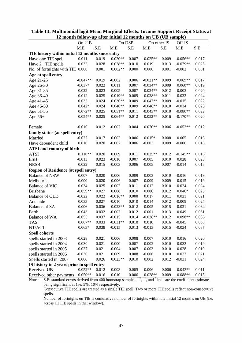
47
Table 13: Multinomial logit Mean Marginal Effects: Income Support Receipt Status at 12 month follow-up after initial 12 months on UB (UB sample)
On U.B On DSP On other IS Off IS M.E S.E M.E S.E M.E S.E M.E S.E TIE history within initial 12 months since entry Have one TIE spell 0.011 0.019 0.020** 0.007 0.025** 0.009 -0.056** 0.017 Have 2+ TIE spells 0.032 0.028 0.028** 0.010 0.019 0.013 -0.079** 0.025 No. of fortnights with TIE 0.000 0.001 0.002** 0.000 0.000 0.001 -0.002 0.001 Age at spell entry Age 21-25 -0.047** 0.019 -0.002 0.006 -0.021** 0.009 0.069** 0.017 Age 26-30 -0.037* 0.022 0.011 0.007 -0.034** 0.009 0.060** 0.019 Age 31-35 0.022 0.023 0.005 0.007 -0.024** 0.012 -0.003 0.020 Age 36-40 -0.012 0.025 0.019** 0.009 -0.038** 0.011 0.032 0.024 Age 41-45 0.032 0.024 0.030** 0.009 -0.047** 0.009 -0.015 0.022 Age 46-50 0.042* 0.024 0.040** 0.009 -0.048** 0.010 -0.034 0.023 Age 51-55 0.072** 0.025 0.051** 0.011 -0.043** 0.010 -0.080** 0.022 Age 56+ 0.054** 0.025 0.064** 0.012 0.052** 0.016 -0.170** 0.020 Female -0.010 0.012 -0.007 0.004 0.070** 0.006 -0.052** 0.012 family status (at spell entry) Married -0.022 0.017 0.002 0.006 0.015* 0.008 0.005 0.016 Have dependent child 0.016 0.020 -0.007 0.006 -0.003 0.009 -0.006 0.018 ATSI and country of birth ATSI 0.110** 0.020 0.009 0.011 0.025** 0.012 -0.145** 0.016 ESB -0.013 0.023 -0.010 0.007 -0.005 0.010 0.028 0.023 NESB 0.022 0.015 -0.003 0.006 -0.005 0.007 -0.014 0.015 Region of Residence (at spell entry) Balance of NSW 0.007 0.020 0.006 0.009 0.003 0.010 -0.016 0.019 Melbourne 0.000 0.020 -0.006 0.007 -0.009 0.009 0.015 0.019 Balance of VIC 0.034 0.025 0.002 0.011 -0.012 0.010 -0.024 0.024 Brisbane -0.059** 0.027 0.008 0.010 0.006 0.012 0.046* 0.025 Balance of QLD -0.022 0.022 -0.016** 0.008 0.017 0.011 0.021 0.021 Adelaide 0.033 0.027 -0.010 0.010 -0.014 0.012 -0.009 0.025 Balance of SA 0.006 0.036 -0.023** 0.012 -0.005 0.015 0.021 0.034 Perth -0.043 0.032 -0.007 0.012 0.001 0.013 0.049 0.031 Balance of WA -0.055 0.037 -0.015 0.014 -0.028** 0.012 0.098** 0.036 TAS 0.067** 0.033 -0.031** 0.010 0.010 0.016 -0.045 0.030 NT/ACT 0.063* 0.038 -0.015 0.013 -0.013 0.015 -0.034 0.037 Spell cohorts spells started in 2003 -0.028 0.021 0.006 0.008 0.007 0.010 0.016 0.020 spells started in 2004 -0.030 0.021 0.000 0.007 -0.002 0.010 0.032 0.019 spells started in 2005 -0.027 0.021 -0.004 0.007 0.003 0.010 0.028 0.019 spells started in 2006 -0.030 0.021 0.009 0.008 -0.006 0.010 0.027 0.021 Spells started in 2007 0.006 0.026 0.023** 0.010 0.002 0.012 -0.031 0.024 IS history in 2 years prior to spell entry Received UB 0.052** 0.012 -0.003 0.005 -0.006 0.006 -0.043** 0.011 Received other payments 0.050** 0.016 0.010 0.006 0.028** 0.009 -0.088** 0.015 Notes: S.E: standard errors derived from 400 bootstrap samples. ***, **, and * indicate the coefficient estimate
being significant at 1%; 5%; 10% respectively. Consecutive TIE spells are treated as a single TIE spell. Two or more TIE spells reflect non-consecutive spells. Number of fortnights on TIE is cumulative number of fortnights within the initial 12 months on UB (i.e. across all TIE spells in that window).
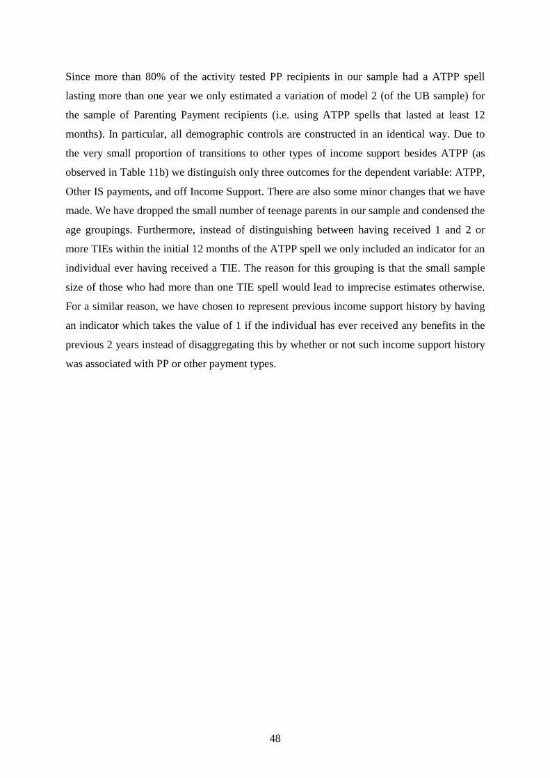
48
Since more than 80% of the activity tested PP recipients in our sample had a ATPP spell
lasting more than one year we only estimated a variation of model 2 (of the UB sample) for
the sample of Parenting Payment recipients (i.e. using ATPP spells that lasted at least 12
months). In particular, all demographic controls are constructed in an identical way. Due to
the very small proportion of transitions to other types of income support besides ATPP (as
observed in Table 11b) we distinguish only three outcomes for the dependent variable: ATPP,
Other IS payments, and off Income Support. There are also some minor changes that we have
made. We have dropped the small number of teenage parents in our sample and condensed the
age groupings. Furthermore, instead of distinguishing between having received 1 and 2 or
more TIEs within the initial 12 months of the ATPP spell we only included an indicator for an
individual ever having received a TIE. The reason for this grouping is that the small sample
size of those who had more than one TIE spell would lead to imprecise estimates otherwise.
For a similar reason, we have chosen to represent previous income support history by having
an indicator which takes the value of 1 if the individual has ever received any benefits in the
previous 2 years instead of disaggregating this by whether or not such income support history
was associated with PP or other payment types.
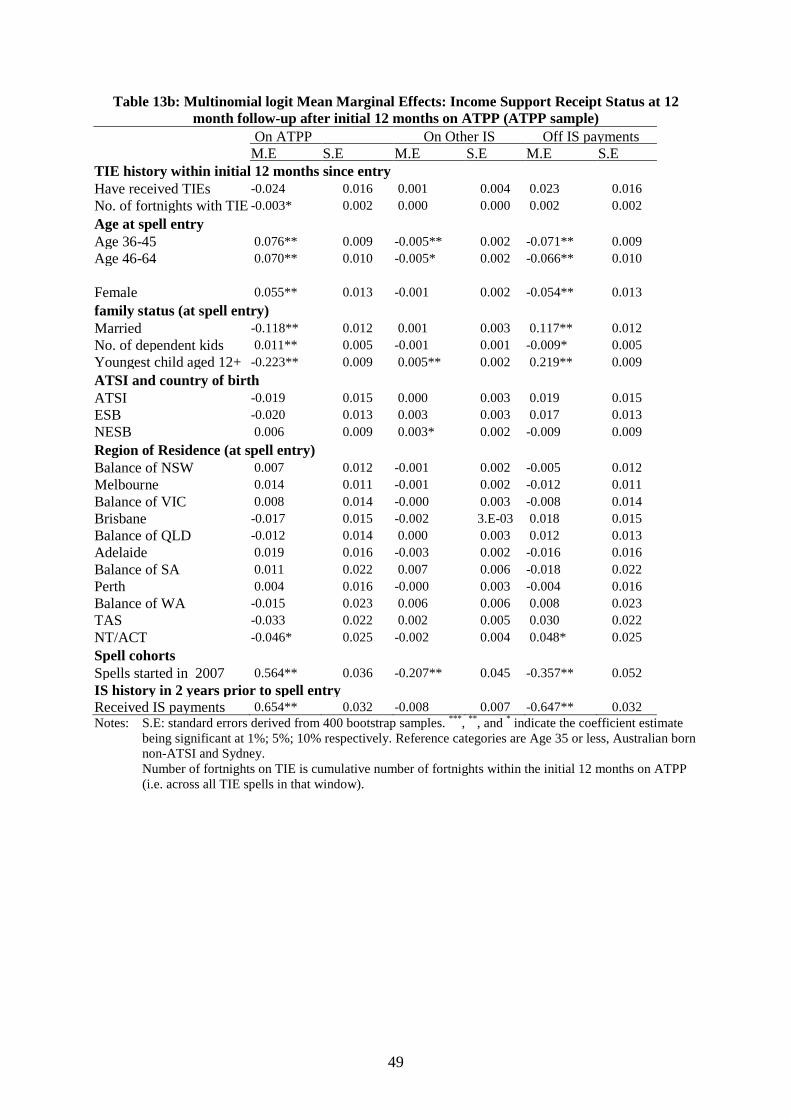
49
Table 13b: Multinomial logit Mean Marginal Effects: Income Support Receipt Status at 12 month follow-up after initial 12 months on ATPP (ATPP sample)
On ATPP On Other IS Off IS payments M.E S.E M.E S.E M.E S.E TIE history within initial 12 months since entry Have received TIEs -0.024 0.016 0.001 0.004 0.023 0.016 No. of fortnights with TIE -0.003* 0.002 0.000 0.000 0.002 0.002 Age at spell entry Age 36-45 0.076** 0.009 -0.005** 0.002 -0.071** 0.009 Age 46-64 0.070** 0.010 -0.005* 0.002 -0.066** 0.010 Female 0.055** 0.013 -0.001 0.002 -0.054** 0.013 family status (at spell entry) Married -0.118** 0.012 0.001 0.003 0.117** 0.012 No. of dependent kids 0.011** 0.005 -0.001 0.001 -0.009* 0.005 Youngest child aged 12+ -0.223** 0.009 0.005** 0.002 0.219** 0.009 ATSI and country of birth ATSI -0.019 0.015 0.000 0.003 0.019 0.015 ESB -0.020 0.013 0.003 0.003 0.017 0.013 NESB 0.006 0.009 0.003* 0.002 -0.009 0.009 Region of Residence (at spell entry) Balance of NSW 0.007 0.012 -0.001 0.002 -0.005 0.012 Melbourne 0.014 0.011 -0.001 0.002 -0.012 0.011 Balance of VIC 0.008 0.014 -0.000 0.003 -0.008 0.014 Brisbane -0.017 0.015 -0.002 3.E-03 0.018 0.015 Balance of QLD -0.012 0.014 0.000 0.003 0.012 0.013 Adelaide 0.019 0.016 -0.003 0.002 -0.016 0.016 Balance of SA 0.011 0.022 0.007 0.006 -0.018 0.022 Perth 0.004 0.016 -0.000 0.003 -0.004 0.016 Balance of WA -0.015 0.023 0.006 0.006 0.008 0.023 TAS -0.033 0.022 0.002 0.005 0.030 0.022 NT/ACT -0.046* 0.025 -0.002 0.004 0.048* 0.025 Spell cohorts Spells started in 2007 0.564** 0.036 -0.207** 0.045 -0.357** 0.052 IS history in 2 years prior to spell entry Received IS payments 0.654** 0.032 -0.008 0.007 -0.647** 0.032 Notes: S.E: standard errors derived from 400 bootstrap samples. ***, **, and * indicate the coefficient estimate
being significant at 1%; 5%; 10% respectively. Reference categories are Age 35 or less, Australian born non-ATSI and Sydney. Number of fortnights on TIE is cumulative number of fortnights within the initial 12 months on ATPP (i.e. across all TIE spells in that window).

50
6. Concluding remarks
This report has mainly investigated the use of Temporary Incapacity Exemptions (TIEs) by
income support customers receiving unemployment benefits, i.e. Newstart or Youth
Allowance (Other) during the period from 1 July 2002 to 30 June 2009. Overall, the majority
of TIEs lasted less than the maximum 13 weeks. However, we do find evidence that usage of
consecutive exemptions is not trivial- over 15% of TIEs lasted 6 months or longer, which are
longer than the duration that typical conditions giving rise to granting a TIE are expected to
last. This is not necessarily a failure of the TIE instrument, but rather signifies that even if a
condition is expected to last less than 6 months the incapacity has its own dynamic.
Furthermore, granting a TIE for at most 13 weeks builds in automatic and periodic
stocktaking moments that allow fine-tuning of the Activity Agreement.
When following a cohort of customers who started an unemployment benefit episode, we
found that those with a TIE history were associated with having a higher probability of
transferring to DSP and a lower probability of being off income support. Although this result
in itself might be expected, it is not clear whether this reflects the health conditions of
individual customers (since some reasons for granting TIEs indicate severe impairment), or
prolonged reliance on income support as a result of exemptions being granted (i.e. interrupted
job search). In all likelihood, it is a combination of both.
The report has also looked at TIE use by individuals on Parenting Payment who were subject
to activity tests. The analysis was undertaken for a much condensed window between 1 July
2006 and 30 June 2009. Overall, the incidence of TIE use is much lower among this group
when compared with those on UB. About 15% of the sampled ATPP recipients had received a
TIE during the observation window, whereas the equivalent for UB recipients is 30%.

51
Appendix Table A1: Multinomial logit coefficient estimates: Income Support Receipt Status at 12-
month follow-up after initial 6 months on UB (UB sample) On DSP On Other IS Off IS Coef. S.E Coef. S.E Coef. S.E TIE history within initial 6 months since spell entry Have one TIE spell 0.906*** 0.174 0.389*** 0.141 -0.332*** 0.078 Have 2+ TIE spells 0.483* 0.277 0.125 0.267 -0.419*** 0.141 No. of fortnights with TIE 0.107*** 0.016 0.002 0.016 -0.008 0.009 Age at spell entry Age 21-25 0.297 0.277 0.035 0.114 0.260*** 0.055 Age 26-30 0.363 0.288 -0.253* 0.143 0.153** 0.064 Age 31-35 0.728*** 0.269 -0.354** 0.148 -0.014 0.067 Age 36-40 1.073*** 0.262 -0.822*** 0.172 0.053 0.071 Age 41-45 1.232*** 0.257 -1.309*** 0.192 0.050 0.073 Age 46-50 1.271*** 0.253 -1.368*** 0.194 -0.090 0.075 Age 51-55 1.522*** 0.252 -1.389*** 0.206 -0.407*** 0.083 Age 56+ 1.807*** 0.244 0.430*** 0.131 -0.743*** 0.083 Female -0.047 0.106 1.337*** 0.080 -0.012 0.037 family status (at spell entry) Married 0.444*** 0.120 0.849*** 0.093 0.186*** 0.053 Have dependent child -0.236 0.152 -0.058 0.122 -0.090 0.062 ATSI and country of birth ATSI 0.229 0.206 0.169 0.122 -0.596*** 0.065 ESB -0.221 0.194 0.125 0.148 0.093 0.071
NESB -0.087 0.132 0.012 0.108 -0.284*** 0.052 Region of Residence (at spell entry) Balance of NSW 0.254 0.168 -0.132 0.128 -0.059 0.062 Melbourne 0.000 0.161 -0.355*** 0.129 0.051 0.059 Balance of VIC -0.283 0.241 -0.225 0.164 -0.236*** 0.079 Brisbane 0.168 0.202 -0.203 0.161 0.230*** 0.075 Balance of QLD -0.406** 0.198 -0.051 0.130 0.167** 0.065 Adelaide 0.040 0.230 -0.326* 0.191 0.008 0.083 Balance of SA -0.350 0.358 0.081 0.206 -0.155 0.111 Perth 0.262 0.241 -0.228 0.195 0.407*** 0.085 Balance of WA -0.301 0.359 -0.179 0.216 -0.001 0.109 TAS -0.729* 0.412 -0.348 0.230 -0.242** 0.111 NT/ACT -0.550 0.418 -0.313 0.248 -0.103 0.119 Spell cohorts spells started in 2003 0.316 0.200 -0.387*** 0.129 0.107* 0.064 spells started in 2004 0.045 0.207 -0.385*** 0.128 0.119* 0.065 spells started in 2005 0.028 0.206 -0.407*** 0.130 0.225*** 0.065 spells started in 2006 0.401** 0.201 -0.589*** 0.137 0.167** 0.067 spells started in 2007 0.504** 0.198 -0.402*** 0.132 -0.016 0.068 spells started in 2008 0.623 0.400 -0.446 0.320 -0.226 0.167 IS history in 2 years prior to spell entry Received UB -0.279*** 0.106 -0.210*** 0.076 -0.328*** 0.036 Received non-UB payments 0.348*** 0.123 0.590*** 0.096 -0.499*** 0.055 constant -4.719*** 0.296 -2.379*** 0.160 0.175** 0.078 Pseudo R2 0.077 Number of obs. 15,859 Notes: ***, **, and * indicate the coefficient estimate being significant at 1%; 5%; 10% respectively.
Consecutive TIE spells are treated as a single TIE spell. Two or more TIE spells reflect non-consecutive spells. Number of fortnights on TIE is cumulative number of fortnights within the initial 6 months on UB (i.e. across all TIE spells in that window).

52
Table A2: Multinomial logit coefficient estimates: Income Support Receipt Status at 12 month follow-up after initial 12 months on UB (UB sample)
On DSP On Other IS Off IS Coef. S.E Coef. S.E Coef. S.E TIE history within initial 12 months since spell entry Have one TIE spell 0.558*** 0.195 0.451*** 0.161 -0.205** 0.086 Have 2+ TIE spells 0.696*** 0.235 0.315 0.248 -0.325** 0.132 No. of fortnights with TIE 0.064*** 0.010 -0.004 0.012 -0.007 0.006 Age at spell entry Age 21-25 -0.014 0.339 -0.264 0.181 0.281*** 0.085 Age 26-30 0.554* 0.314 -0.575** 0.230 0.239** 0.096 Age 31-35 0.222 0.333 -0.443** 0.219 -0.045 0.101 Age 36-40 0.752** 0.316 -0.744*** 0.251 0.116 0.106 Age 41-45 0.960*** 0.299 -1.099*** 0.259 -0.098 0.109 Age 46-50 1.138*** 0.294 -1.150*** 0.267 -0.178 0.112 Age 51-55 1.291*** 0.295 -1.028*** 0.267 -0.395*** 0.119 Age 56+ 1.520*** 0.290 0.513*** 0.187 -0.806*** 0.124 Female -0.154 0.134 1.366*** 0.120 -0.155*** 0.056 Family status (at spell entry) Married 0.083 0.161 0.323** 0.142 0.051 0.078 Have dependent child -0.245 0.200 -0.096 0.189 -0.044 0.091 ATSI and country of birth ATSI 0.079 0.264 0.265 0.176 -0.738*** 0.100 ESB -0.304 0.256 -0.089 0.229 0.107 0.106 NESB -0.124 0.172 -0.141 0.168 -0.078 0.077 Region of Residence (at spell entry) Balance of NSW 0.121 0.209 0.040 0.194 -0.066 0.093 Melbourne -0.170 0.201 -0.188 0.199 0.049 0.087 Balance of VIC 0.001 0.261 -0.318 0.257 -0.138 0.117 Brisbane 0.272 0.253 0.207 0.236 0.247** 0.114 Balance of QLD -0.453* 0.250 0.331* 0.195 0.107 0.100 Adelaide -0.340 0.308 -0.369 0.293 -0.080 0.125 Balance of SA -0.791 0.541 -0.116 0.338 0.062 0.162 Perth -0.106 0.328 0.081 0.280 0.228* 0.130 Balance of WA -0.376 0.494 -0.663 0.427 0.388** 0.160 TAS -1.360** 0.611 0.063 0.298 -0.262 0.160 NT/ACT -0.549 0.500 -0.395 0.377 -0.213 0.181 Spell cohorts spells started in 2003 0.221 0.240 0.172 0.200 0.097 0.092 spells started in 2004 0.058 0.247 0.006 0.205 0.153* 0.092 spells started in 2005 -0.077 0.251 0.109 0.205 0.136 0.093 spells started in 2006 0.293 0.244 -0.071 0.211 0.136 0.095 spells started in 2007 0.553** 0.258 0.037 0.234 -0.123 0.113 IS history in 2 years prior to spell entry Received UB -0.177 0.133 -0.203* 0.114 -0.225*** 0.054 Received other payments 0.181 0.158 0.423*** 0.140 -0.393*** 0.079 constant -4.041*** 0.351 -3.031*** 0.256 -0.203* 0.117 Pseudo R2 0.072 Number of obs. 7,617 Notes: ***, **, and * indicate the coefficient estimate being significant at 1%; 5%; 10% respectively.
Consecutive TIE spells are treated as a single TIE spell. Two or more TIE spells reflect non-consecutive spells. Number of fortnights on TIE is cumulative number of fortnights within the initial 12 months on UB (i.e. across all TIE spells in that window).

53
Table A2b: Multinomial logit coefficient estimates: Income Support Receipt Status at 12 month follow-up after initial 12 months on ATPP (ATPP sample)
On other IS Off IS payments Coef. S.E Coef. S.E TIE history within initial 12 months since spell entry Have one TIE spell 0.221 0.398 0.129 0.080 No. of fortnights with TIE 0.035 0.036 0.014* 0.008 Age at spell entry Age 36-45 -0.868*** 0.236 -0.400*** 0.046 Age 46-64 -0.765** 0.299 -0.366*** 0.057 Female -0.317 0.336 -0.289*** 0.067 Family status (at spell entry) Married 0.490 0.329 0.604*** 0.057 No. of dependent kids -0.241 0.150 -0.056** 0.027 Youngest child aged 12+ 1.168*** 0.248 1.109*** 0.043 ATSI and country of birth ATSI 0.131 0.434 0.105 0.082 ESB 0.516 0.340 0.101 0.069 NESB 0.479* 0.266 -0.044 0.053 Region of Residence (at spell entry) Balance of NSW -0.227 0.365 -0.033 0.067 Melbourne -0.234 0.325 -0.073 0.062 Balance of VIC -0.059 0.434 -0.045 0.081 Brisbane -0.233 0.444 0.097 0.079 Balance of QLD 0.056 0.370 0.066 0.072 Adelaide -0.563 0.563 -0.097 0.089 Balance of SA 0.706 0.526 -0.085 0.126 Perth -0.066 0.452 -0.024 0.087 Balance of WA 0.693 0.489 0.061 0.125 TAS 0.396 0.565 0.169 0.111 NT/ACT -0.189 0.769 0.252* 0.131 Spell cohorts Spells started in 2007 -5.471*** 0.364 -2.520*** 0.267 IS history in 2 years prior to spell entry Received IS -3.422*** 0.563 -3.689*** 0.400 constant 4.481*** 0.742 5.313*** 0.481 Pseudo R2 0.074 Number of obs. 16,563 Notes: ***, **, and * indicate the coefficient estimate being significant at 1%; 5%; 10% respectively.
Number of fortnights on TIE is cumulative number of fortnights within the initial 12 months on ATPP (i.e. across all TIE spells in that window).
Related Documents