FINAL REPORT New Cost-Effective Method for Long-Term Groundwater Monitoring Programs SERDP Project ER-1601 May 2013 Charles J. Newell David Adamson Thomas E. McHugh Michal Rysz GSI Environmental Inc.

Welcome message from author
This document is posted to help you gain knowledge. Please leave a comment to let me know what you think about it! Share it to your friends and learn new things together.
Transcript

FINAL REPORT New Cost-Effective Method for Long-Term Groundwater
Monitoring Programs
SERDP Project ER-1601
May 2013
Charles J. Newell David Adamson Thomas E. McHugh Michal Rysz GSI Environmental Inc.

This report was prepared under contract to the Department of Defense Strategic Environmental Research and Development Program (SERDP). The publication of this report does not indicate endorsement by the Department of Defense, nor should the contents be construed as reflecting the official policy or position of the Department of Defense. Reference herein to any specific commercial product, process, or service by trade name, trademark, manufacturer, or otherwise, does not necessarily constitute or imply its endorsement, recommendation, or favoring by the Department of Defense.

REPORT DOCUMENTATION PAGE Form Approved
OMB No. 0704-0188 Public reporting burden for this collection of information is estimated to average 1 hour per response, including the time for reviewing instructions, searching existing data sources, gathering and maintaining the data needed, and completing and reviewing this collection of information. Send comments regarding this burden estimate or any other aspect of this collection of information, including suggestions for reducing this burden to Department of Defense, Washington Headquarters Services, Directorate for Information Operations and Reports (0704-0188), 1215 Jefferson Davis Highway, Suite 1204, Arlington, VA 22202-4302. Respondents should be aware that notwithstanding any other provision of law, no person shall be subject to any penalty for failing to comply with a collection of information if it does not display a currently valid OMB control number. PLEASE DO NOT RETURN YOUR FORM TO THE ABOVE ADDRESS.
1. REPORT DATE (03-01-2013)
2. REPORT TYPE Technical
3. DATES COVERED (From - To) September 2008 – present
4. TITLE AND SUBTITLE
5a. CONTRACT NUMBER W912HQ-08-C-0057
New Cost-Effective Method for Long-Term Groundwater Monitoring Programs
5b. GRANT NUMBER
5c. PROGRAM ELEMENT NUMBER
6. AUTHOR(S) Newell, Charles J., Adamson, David T., McHugh, Thomas E., Rysz, Michal W.
5d. PROJECT NUMBER ER-1601
5e. TASK NUMBER
5f. WORK UNIT NUMBER
7. PERFORMING ORGANIZATION NAME(S) AND ADDRESS(ES)
8. PERFORMING ORGANIZATION REPORT
GSI Environmental Inc 2211 Norfolk Houston, TX 77098
1
9. SPONSORING / MONITORING AGENCY NAME(S) AND ADDRESS(ES) 10. SPONSOR/MONITOR’S ACRONYM(S) SERDP
11. SPONSOR/MONITOR’S REPORT
NUMBER(S)
12. DISTRIBUTION / AVAILABILITY STATEMENT
13. SUPPLEMENTARY NOTES
14. ABSTRACT This project involved basic research on an alternative groundwater sampling approach—vapor-phase groundwater monitoring—that relies on a different set of physical processes and analytical instruments to provide the Department of Defense (DoD) with reliable and accurate long-term monitoring for volatile organic compounds (VOCs). The overall goal of this research project is to evaluate the utility of on-site vapor-phase analysis of samples from a groundwater monitoring well as an alternative to off-site analysis of groundwater samples. Current approaches for long-term groundwater monitoring programs rely on water sampling and analysis using traditional decades-old protocols that are time-consuming and costly. Complying with the requirements of these monitoring programs comprise a significant portion of life-cycle remediation costs the for Department of Defense (DoD). There is an opportunity to use existing vapor-phase based technologies as part of a new approach that generates monitoring data more rapidly at a lower overall cost.
15. SUBJECT TERMS Long-term monitoring, optimization, cost-effectiveness, vapor-phase monitoring, groundwater monitoring, in-well mixing, stratification, passive vapor diffusion samplers
16. SECURITY CLASSIFICATION OF:
17. LIMITATION OF ABSTRACT
18
19a. NAME OF RESPONSIBLE PERSON
a. REPORT
b. ABSTRACT
c. THIS PAGE
19b. TELEPHONE NUMBER (include area code)
Standard Form 298 (Rev. 8-98)Prescribed by ANSI Std. Z39.18
May 2013
SERDP ER-1601 ii Final Report
TABLE OF CONTENTS
TABLE OF CONTENTS ............................................................................................................. ii LIST OF FIGURES ...................................................................................................................... v
LIST OF TABLES ..................................................................................................................... viii LIST OF ACRONYMS ................................................................................................................ x KEYWORDS ................................................................................................................................ xi ACKNOWLEDGEMENTS ....................................................................................................... xii ABSTRACT ........................................................................................................................... …....1
1. OBJECTIVE ............................................................................................................................ 4
2. BACKGROUND ...................................................................................................................... 6
2.1 SERDP Relevance .............................................................................................................. 6 2.2 Technical Rationale ........................................................................................................... 7 2.3 Monitoring Approaches Tested During Laboratory Validation Study ...................... 10 2.3.1 Vapor-Phase Monitoring Equipment ............................................................................... 10
2.3.2 Vapor-Phase Sampling Methods ..................................................................................... 11 2.4 Monitoring Approaches for Field Testing ..................................................................... 13 2.4.1 Vapor-Phase Sampling Methods ..................................................................................... 13
2.4.2 Water-Phase Sampling Methods ..................................................................................... 17 2.5 Potential Influence of Temperature Gradients on Monitoring ................................... 19
3. MATERIALS AND METHODS .......................................................................................... 22
3.1 Laboratory Validation Study .......................................................................................... 23 3.1.1 Portable Field Instrument Validation .............................................................................. 24
3.1.2 Validation of Headspace Analysis Method ..................................................................... 24
3.1.3 Validation of Vapor-Phase Sampling Methods ............................................................... 26
3.2 Temperature Study .......................................................................................................... 29 3.3 Field Programs (Preliminary, Expanded, and Supplemental) ..................................... 31 3.3.1 Site Selection ................................................................................................................... 31
3.3.2 Sampling Methods ........................................................................................................... 31
3.3.3 Analytical Methods ......................................................................................................... 38
3.3.4 Sampling and Analysis Plans .......................................................................................... 39
3.4 Data Analysis ................................................................................................................... 45

May 2013
SERDP ER-1601 iii Final Report
3.4.1 Conversion of Vapor Concentration to Groundwater Concentration .............................. 45
3.4.2 Data Transformations ...................................................................................................... 46
3.4.3 Linear Regression Analysis ............................................................................................. 47
3.4.4 Two Sample Tests ........................................................................................................... 47
3.4.5 Relative Percent Difference and Relative Standard Deviation (Coefficient of Variation) .................................................................................................................................................. 48
3.4.6 Analysis of Variance (ANOVA) ..................................................................................... 49
4. RESULTS AND DISCUSSION ............................................................................................ 51
4.1 Laboratory Validation Study .......................................................................................... 52 4.1.1 Portable Field Instrument Validation Results ................................................................. 52 4.1.2 Headspace Sampling Method Validation Results ........................................................... 55
4.1.3 Vapor-Phase Sampling Method Validation Results ........................................................ 57
4.2 Temperature Study ......................................................................................................... 60 4.2.1 Temperature Data ............................................................................................................ 60
4.2.2 VOC Concentration Data ................................................................................................ 61
4.3 Preliminary Field Program ............................................................................................ 66 4.3.1 Well Characteristics and Sampling Data ......................................................................... 67 4.3.2 Comparison of Vapor-Phase Based Methods to Low-Flow and Passive Groundwater Sampling .................................................................................................................................. 70 4.3.3 Field Analysis of Groundwater Samples (Field Equilibration Method) ......................... 78 4.3.4 Evaluation of Precision and Accuracy for Field and Lab Analyses ................................ 80 4.3.5 Summary of Factors Contributing to Bias and Variability .............................................. 84 4.3.6 Project Implications for Further Field Testing ................................................................ 87 4.4 Expanded Field Program ................................................................................................ 90 4.4.1 Well Characteristics and Sampling Data ......................................................................... 90 4.4.2 Comparison of Passive Vapor Diffusion Sampling to Low-Flow Groundwater Sampling .................................................................................................................................................. 91 4.4.3 Field Analysis of Groundwater Samples (Field Equilibration Method) ....................... 100 4.4.4 Comparison of Individual Vapor-Phase Based Sampling Methods .............................. 102 4.4.5 Evaluation of Precision and Accuracy for Field and Lab Analyses .............................. 103 4.4.6 Summary of Factors Contributing to Bias and Variability ............................................ 107 4.5 Supplemental Field Program ....................................................................................... 116 4.5.1 Well Characteristics and Sampling Data ....................................................................... 116 4.5.2 Variability Associated with Vapor-Phase Based Sampling Methods .......................... 118
May 2013
SERDP ER-1601 iv Final Report
4.5.3 Variablity of Vapor-Phase Based Sampling Methods Relative to Groundwater Sampling Methods .................................................................................................................................. 119 4.5.4 Comparison of Concentrations Obtained using Vapor-Phase Based Sampling Methods vs. Groundwater Sampling Methods ...................................................................................... 122 4.5.5 Influence of Spatial and Temporal Variablity in Monitoring Data ............................... 129 4.6 Assessment of Cost-Effectiveness ................................................................................. 135 4.6.1 Cost Elements ................................................................................................................ 136 4.6.2 Cost Model .................................................................................................................... 137 4.6.3 Results ........................................................................................................................... 138 4.6.4 Sensitivity Analysis ....................................................................................................... 142
5. CONCLUSIONS AND IMPLICATIONS FOR FUTURE RESEARCH/ IMPLEMENTATION .............................................................................................................. 144
5.1 Key Conclusions ............................................................................................................ 144 5.2 Discussion ....................................................................................................................... 145
6. LITERATURE CITED ....................................................................................................... 154
APPENDIX A: SUPPORTING DATA APPENDIX B: LIST OF SCIENTIFIC/TECHNICAL PUBLICATIONS APPENDIX C: OTHER SUPPORTING MATERIALS
May 2013
SERDP ER-1601 v Final Report
LIST OF FIGURES
Figure 2.1. Technical Approach for Vapor-Phase Based Groundwater Monitoring. ................ 7
Figure 2.2. Well Vapor Sampling Approaches Tested During Laboratory Validation Study 12
Figure 2.3. Guidance for Determining if Pressure Adjustments are Necessary for Various Vapor-Phase Based Groundwater Monitoring Methods. ...................................... 16
Figure 3.1. Portable field instruments used for the detection of vapor-phase volatile organic compounds. ........................................................................................................... 24
Figure 3.2. Reactors constructed for the validation of the sampling tube technique validation............................................................................................................................... 27
Figure 3.3. Passive vapor diffusion (PVD) samplers and reactors used for passive technique validation............................................................................................................... 28
Figure 3.4. Simplified cross-section for monitoring wells included in temperature study ..... 30
Figure 3.5. Sampling Methods Tested During Preliminary Field Program ............................ 34
Figure 3.6. Sampling Protocol During Preliminary Field Program ........................................ 34
Figure 3.7. Passive Vapor Diffusion (PVD) Sampler ............................................................. 36
Figure 3.8. Field Equilibration Method (On-Site Analysis of Vapor in Equilibrium with Low-Flow Groundwater Sample Collected from Well Screen) .................................... 36
Figure 4.1. VOC Concentration vs. Time in Headspace of Equilibration Reactor ................. 55
Figure 4.2. TCE Concentration Inside PVD Samplers During Laboratory Validation Study ............................................................................................................................... 59
Figure 4.3. Measured and Predicted Groundwater Temperature Over Monitoring Period During Temperature Study ................................................................................... 61
Figure 4.4. TCE Concentration Data Collected from Two Monitoring Wells During Temperature Study ................................................................................................ 63
Figure 4.5. Predicted Vertical Temperature Gradients and Resulting Mixing Conditions in Groundwater Monitoring Wells During Temperature Study ................................ 65
Figure 4.6. Example of Groundwater In-Well Mixing Samplers ............................................ 66
Figure 4.7. Passive Vapor Diffusion (PVD) Samplers vs. Low-Flow Groundwater Samples During Preliminary Field Program ....................................................................... 71
Figure 4.8. Passive Diffusion Bags at Screen vs. Low-Flow Groundwater Samples During Preliminary Field Program .................................................................................... 71
May 2013
SERDP ER-1601 vi Final Report
Figure 4.9. Passive Vapor Diffusion (PVD) Samplers vs. Passive Diffusion Bags at Screen During Preliminary Field Program ....................................................................... 72
Figure 4.10a. Headspace Samples from Water-Vapor Interface (GC Analysis) vs. Low-Flow Groundwater Samples During Preliminary Field Program ................................... 73
Figure 4.10b. Headspace Samples from Water-Vapor Interface (PID Analysis) vs. Low-Flow Groundwater Samples During Preliminary Field Program ................................... 74
Figure 4.11a. Passive Diffusion Bags at Water-Vapor Interface vs. Low-Flow Groundwater Samples During Preliminary Field Program ......................................................... 75
Figure 4.11b. Headspace Samples from Water-Vapor Interface (GC Analysis) vs. Passive Diffusion Bags at Water-Vapor Interface During Preliminary Field Program ..... 76
Figure 4.12a. Headspace Samples from Upper Portion of Well (GC Analysis) vs. Low-Flow Groundwater Samples During Preliminary Field Program ................................... 77
Figure 4.12b. Headspace Samples from Upper Portion of Well (PID Analysis) vs. Low-Flow Groundwater Samples During Preliminary Field Program ................................... 77
Figure 4.13. Headspace Samples from Upper Portion of Well vs. Headspace Samples from Water-Vapor Interface (GC Analysis) During Preliminary Field Program .......... 78
Figure 4.14. Field GC Analysis of Vapor in Equilibrum with Groundwater Samples vs. Lab Analysis of Groundwater Samples During Preliminary Field Program ............... 79
Figure 4.15. Field PID Analysis vs. Field GC Analysis of Headspace Samples During Preliminary Field Program .................................................................................... 81
Figure 4.16a. Field GC Analysis vs. Laboratory Analysis of Headspace Samples .................... 82
Figure 4.16b. Field PID Analysis vs. Laboratory Analysis of Headspace Samples ................... 83
Figure 4.17. Laboratory Analysis of Headspace Samples from Upper Portion of Well vs. Headspace Samples from Water-Vapor Interface ................................................. 83
Figure 4.18. Passive Diffusion Bags at Water-Vapor Interface vs. Passive Diffusion Bags at Screen During Preliminary Field Program .......................................................... 86
Figure 4.19. Correlation between Normalized Concentration During Preliminary Field Program vs. A) Distance from Top of Aquifer to Screen; and B) Depth to Top of Aquifer ................................................................................................................. 87
Figure 4.20. Overview of Bias (Slope) and Variability (R2) Observed in Sampling Methods During Preliminary Field Program ....................................................................... 88
Figure 4.21. Short Passive Vapor Diffusion (PVD) Samplers vs. Low-Flow Groundwater Samples During Expanded Field Program ............................................................ 92
Figure 4.22. GSI Extended-Length Passive Vapor Diffusion (PVD) Samplers (GC Analysis) vs. Low-Flow Groundwater Samples During Expanded Field Program .............. 94
May 2013
SERDP ER-1601 vii Final Report
Figure 4.23. GSI Extended-Length Passive Vapor Diffusion (PVD) Samplers (PID Analysis) vs. Low-Flow Groundwater Samples During Expanded Field Program .............. 95
Figure 4.24. GSI Extended-Length Passive Vapor Diffusion (PVD) Samplers (HAPSITE Analysis) vs. Low-Flow Groundwater Samples During Expanded Field Program............................................................................................................................... 96
Figure 4.25. Haas Balloon Passive Vapor Diffusion (PVD) Samplers (GC Analysis) vs. Low-Flow Groundwater Samples During Expanded Field Program ............................ 98
Figure 4.26. Haas Balloon Passive Vapor Diffusion (PVD) Samplers (PID Analysis) vs. Low-Flow Groundwater Samples During Expanded Field Program ............................ 99
Figure 4.27. Haas Balloon Passive Vapor Diffusion (PVD) Samplers (HAPSITE Analysis) vs. Low-Flow Groundwater Samples During Expanded Field Program .................. 100
Figure 4.28. Field GC Analysis of Vapor in Equilibrium with Groundwater Samples vs. Lab Analysis of Groundwater Samples During Expanded Field Program ................ 101
Figure 4.29. Field HAPSITE Analysis of Vapor in Equilibrium with Groundwater Samples vs. Lab Analysis of Groundwater Samples During Expanded Field Program ......... 101
Figure 4.30. Field PID Analyses vs. Field GC Analyses of Samples Collected During Expanded Field Program ..................................................................................... 106
Figure 4.31. HAPSITE Analyses vs. Field GC Analyses of Samples Collected During Expanded Field Program ..................................................................................... 107
Figure 4.32. Variability Associated with Vapor-Phase Based Sampling Methods Relative to Groundwater Sampling Methods During Supplemental Field Program ............. 121
Figure 4.33. Relative Percent Difference Between Vapor-Phase Based Sampling Methods and Groundwater Method During Supplemental Field Program. .............................. 127
Figure 4.34. All Concentration Data from PVD Samplers During Supplemental Field Program............................................................................................................................. 131
Figure 4.35. Concentration Data from PVD Samplers During Supplemental Field Program Grouped by Event ............................................................................................... 132
Figure 4.36. Cost Scenarios ..................................................................................................... 137
Figure 4.37. Summary of Cost Sensitivity Analysis ............................................................... 141
May 2013
SERDP ER-1601 viii Final Report
LIST OF TABLES
Table 3.1. Test Conditions for Headspace Sampling Method .................................................. 26
Table 3.2. Primary Site Selection Criteria ................................................................................ 31
Table 3.3. Sites and Wells Selected for Field Programs ........................................................... 32
Table 3.4. Summary of Sampling Method Used During Field Programs ................................. 32
Table 3.5. Sampling Events for Preliminary Field Program ..................................................... 40
Table 3.6. Sampling and Analysis Plan for Preliminary Field Program ................................... 40
Table 3.7. Sampling Events for Expanded Field Program ........................................................ 41
Table 3.8. Sampling and Analysis Plan for Expanded Field Program ...................................... 42
Table 3.9. Summary of Supplemental Field Program: Joint Field Program with SERDP ER-1705.......................................................................................................................... 44
Table 4.1. Accuracy, Precision, and Sensitivity of ppb RAE 3000 PID ................................... 53
Table 4.2. Accuracy, Precision, and Sensitivity of Voyager GC P503 ..................................... 54
Table 4.3. Accuracy, Precision, and Sensitivity of Voyager GC P505 ..................................... 55
Table 4.4. Accuracy and Precision of Headspace Analysis Method Using Voyager GC During Laboratory Validation Study (Single VOC Reactors) ............................................. 56
Table 4.5. Accuracy and Precision of Headspace Analysis Method Using Voyager GC During Laboratory Validation Study (VOC Mixture Reactors) ........................................... 56
Table 4.6. Evaluation of Tube with Membrane Sampling Method During Laboratory Validation Study ...................................................................................................... 58
Table 4.7. Accuracy of PVD Sampling Method During Laboratory Validation Study ............ 59
Table 4.8. Summary of Samples Collected and Analyzed During Preliminary Field Program.................................................................................................................................. 68
Table 4.9. Calculated and Measured Groundwater Concentrations for Samples Collected During Preliminary Field Study ............................................................................... 69
Table 4.10. Precision of Laboratory vs. Field Analyses of Duplicate Samples During Preliminary Field Program ....................................................................................... 80
Table 4.11. Precision of Replicate Field Analyses of All Samples ............................................ 80
Table 4.12. Summary of Data Evaluation for All Sampling Methods Used During Preliminary Field Program........................................................................................................... 89
Table 4.13. Summary of Samples Collected and Analyzed During Expanded Field Program .. 90

May 2013
SERDP ER-1601 ix Final Report
Table 4.14. Summary of Data Evaluation for All Sampling Methods Used During Expanded Field Program......................................................................................................... 104
Table 4.15. Precision of Laboratory vs. Field Analyses of Duplicate Samples During Expanded Field Program......................................................................................................... 103
Table 4.16. Precision of Replicate Field Analyses of All Samples During Expanded Field Program .................................................................................................................. 105
Table 4.17. Precision of Inter-Event Monitoring Data from Same Wells During Expanded Field Program .................................................................................................................. 105
Table 4.18. Effect of Aquifer Characteristics on Variability Between Calculated and Measured Groundwater Concentrations During Expanded Field Study ................................ 112
Table 4.19. Effect of Aquifer Characteristics on Bias Between Calculated and Measured Groundwater Concentrations During Expanded Field Study ................................ 113
Table 4.20. Summary of Data Evaluation for All Sampling Methods Used During Expanded Field Study: Wells in Confined Aquifers ............................................................... 114
Table 4.21. Summary of Data Evaluation for All Sampling Methods Used During Expanded Field Study: Wells in Unconfined Aquifers ........................................................... 115
Table 4.22. Datasets Generated During Supplemental Field Program: Joint Program with SERDP ER-1705 .................................................................................................... 117
Table 4.23. Variability Associated with Vapor-Phase Based Sampling Methods During Supplemental Field Program .................................................................................. 118
Table 4.24. Variability Associated with Vapor-Phase Based Sampling Methods Relative to Groundwater Sampling Methods During Supplemental Field Program ................ 120
Table 4.25. Summary of Data Evaluation for All Sampling Methods Used During Supplemental Field Program......................................................................................................... 126
Table 4.26. Variability Associated with Individual Wells Included in Supplemental Field Program .................................................................................................................. 129
Table 4.27. Evaluation of Stratification in Wells Included in Supplemental Field Program ... 134
Table 4.28. Cost Elements Associated with Long-Term Groundwater Monitoring ................. 136
Table 4.29. Summary of Cost Modeling Results ...................................................................... 140
May 2013
SERDP ER-1601 x Final Report
LIST OF ACRONYMS
AFCEE ............................................................. Air Force Center for Environmental Excellence ANOVA ........................................................................................................ Analysis of Variance CV ................................................................................................... Coefficient of Variation CVOC ........................................................................ Chlorinated Volatile Organic Compound DCE ................................................................................................................. Dichloroethene DoD .................................................................................................... Department of Defense ECD ............................................................................................... Electron Capture Detector EDQW ......................................................................... Environmental Data Quality Workgroup EPA ................................................................................... Environmental Protection Agency ESTCP .................................... Environmental Security and Technology Certification Program GC ......................................................................................................... Gas Chromatograph gpm ............................................................................................................ gallons per minute GSI ................................................................................................... GSI Environmental Inc. GW .................................................................................................................... Groundwater HDPE .............................................................................................. High-Density Polyethylene ITRC ............................................................... Interstate Technology and Regulatory Council LDPE .............................................................................................. Low-Density Polyethylene LF ........................................................................................................................ Low-Flow MCL ......................................................................................... Maximum Contaminant Level MDL .................................................................................................. Method Detection Limit MS ........................................................................................................... Mass Spectrometer PCE ............................................................................................................ Tetrachloroethene ppbv ................................................................................................... parts per billion volume PDB ..................................................................................... Passive Diffusion Bag [Sampler] PID ................................................................................................. Photoionization Detector PPS ............................................................................................ Purge to Parameter Stability PVA ................................................................................................. Portable Vapor Analyzer PVC ........................................................................................................... Polyvinyl Chloride PVD ................................................................................. Passive Vapor Diffusion [Sampler] QA/QC ................................................................................. Quality Assurance/Quality Control RPD ............................................................................................. Relative Percent Difference RSD ............................................................................................ Relative Standard Deviation SERDP ....................................... Strategic Environmental Research and Development Program TCE ................................................................................................................ Trichloroethene USGS ........................................................................................ United States Geologic Survey VC ................................................................................................................. Vinyl Chloride VOC ............................................................................................ Volatile Organic Compound WVI ..................................................................................................... Water-Vapor Interface
May 2013
SERDP ER-1601 xi Final Report
KEYWORDS
Long-term monitoring, optimization, cost-effectiveness, vapor-phase monitoring, groundwater monitoring, in-well mixing, stratification, passive vapor diffusion samplers
May 2013
SERDP ER-1601 xii Final Report
ACKNOWLEDGEMENTS
GSI Environmental, Inc. (GSI) has completed a combination of laboratory and field studies as part of the SERDP-funded environmental restoration project SERDP ER-1601. Results and conclusions from this work are presented as part of this final project report. The main goal of this project is to determine whether vapor-phase measurements of headspace in a monitoring well conducted using field-portable equipment can serve as a reliable and accurate long-term method for monitoring volatile organic compounds (VOCs) in groundwater. Investigators at GSI for this project included Dr. Charles Newell (Principal Investigator), Dr. David Adamson, Dr. Tom McHugh, Dr. Michal Rysz, Roberto Landazuri, and Dr. Ahmad Seyedabbasi. Dr. Adamson served as the project manager, and Dr. Rysz and Mr. Landazuri of GSI were responsible for designing field equipment and implementing the program. Laboratory work was completed at Rice University in cooperation with Dr. Pedro Alvarez, chair of the Civil and Environmental Engineering Department. The majority of field studies were performed at a number of commercial/industrial sites in the greater Houston, Texas area, and the authors gratefully acknowledge the participation and cooperation of the respective site managers. Technical support and sampling equipment for a portion of the project came from Patrick Haas (P.E. Haas & Associates, LLC).
May 2013
SERDP ER-1601 1 Final Report
ABSTRACT
What We Learned
1. Existing commercially available field-portable vapor-phase monitoring equipment are sufficiently accurate, precise, and sensitive for calculating equivalent VOC concentrations in groundwater down to part per billion levels.
2. VOC groundwater concentrations can be reasonably and reliably estimated using submerged passive vapor samplers. Both a simple passive vapor sampler constructed of a 40-mL vial in plastic and the Haas Balloon Sampler worked well. Field equilibration of conventional collected groundwater samples followed by on-site vapor analysis using a field GC also worked well.
3. A field-portable GC demonstrated the highest performance of the analytical devices that were tested. Simple PID instruments did not work well for this application.
4. Vapor-phase sampling and analysis methods are easy to implement and can be tailored to site-specific needs.
What Doesn’t Work
5. Collecting vapor samples from a sealed monitoring well headspace was not an effective method for determining groundwater concentrations under the tested conditions due to stratification in wells (see Result 8).
6. Vapor-phase based monitoring methods are no more variable than conventional groundwater monitoring methods, including low flow sampling.
Key Things to Watch Out For
7. Although not a strong factor in this study, seasonal temperature gradients have the potential to significantly alter monitoring data, including both conventional and vapor-phase based methods.
8. Vertical stratification can be important contributing factor to variability and limits the utility of the well-headspace vapor-phase-based monitoring approach.
9. Other well and aquifer-specific factors can contribute to variability and influence the performance of vapor-phase based monitoring methods.
Key Conclusions
10. Passive vapor sampling methods represent a very promising approach for field-based estimation of groundwater concentrations.
11. Vapor-phase based methods represent a significant cost savings (36% or more) relative to conventional groundwater monitoring approaches.
May 2013
SERDP ER-1601 2 Final Report
OBJECTIVE: This project involved basic research on an alternative groundwater sampling approach—vapor-phase groundwater monitoring—that relies on a different set of physical processes and analytical instruments to provide the Department of Defense (DoD) with reliable and accurate long-term monitoring for volatile organic compounds (VOCs). The overall goal of this research project is to evaluate the utility of on-site vapor-phase analysis of samples from a groundwater monitoring well as an alternative to off-site analysis of groundwater samples. Current approaches for long-term groundwater monitoring programs rely on water sampling and analysis using traditional decades-old protocols that are time-consuming and costly. Complying with the requirements of these monitoring programs comprise a significant portion of life-cycle remediation costs the for Department of Defense (DoD). There is an opportunity to use existing vapor-phase based technologies as part of a new approach that generates monitoring data more rapidly at a lower overall cost.
TECHNICAL APPROACH: All investigations completed as part of this project were designed to test the principle that the VOC concentration measured in a vapor-phase sample in equilibrium with affected groundwater can be used to accurately determine the VOC concentration in the associated groundwater at or below maximum contaminant levels (MCLs). Two key hypotheses were developed to support this principle: (1) Portable vapor-phase monitoring instruments can be used to accurately determine VOC concentrations in water under equilibrium conditions; (2) In-well mixing is sufficient in some or all groundwater monitoring wells to establish equilibrium partitioning conditions between affected groundwater and in-well headspace vapors. These hypotheses were tested through a series of laboratory and field-based programs, consisting of: i) a laboratory-based study to validate analytical equipment and to identify promising methods; ii) three distinct phases of field-based studies to test various sampling and collection methods and to examine design and well-specific factors that influenced performance; and iii) a combined modeling-field study that focused on the influence of seasonal temperature gradients on vertical stratification of concentration within monitoring wells. A variety of vapor-phase sampling and/or analysis techniques were tested, including: i) direct sampling and analysis from the headspace of a capped monitoring well; ii) several different permutations of submerged passive vapor diffusion samplers, all of which are gas-permeable but water tight; and iii) “field equilibration” of groundwater (collected using low-flow techniques) in a vial, followed by on-site analysis of the equilibrated headspace. A combination of quantitative methods was used to evaluate vapor-phase based concentration data to more conventional (baseline) groundwater concentration data. These evaluation methods and metrics included linear regression, relative percent difference, coefficient of variation, ANOVA, and parametric and non-parametric statistical tests for significance. The vast majority of the validation data were collected in the field, with approximately 1100 concentration datapoints collected during the various field programs.
RESULTS: The project findings confirmed that existing field-portable vapor-phase monitoring equipment are sufficiently accurate, precise, and sensitive for calculating equivalent VOC concentrations in groundwater. Specifically, a field-portable gas chromatograph (GC) demonstrated the highest performance of the analytical devices that were tested. Alternative field instruments for vapor-phase analysis—a simple PID-based handheld meter and the HAPSITE with GC/MS capabilities—were also tested during one or more of the field programs. These

May 2013
SERDP ER-1601 3 Final Report
instruments did not perform as strongly as the field GC with respect to accuracy and precision, although the HAPSITE did prove useful in terms of identifying a higher number of constituents at lower detection limits. Vapor-phase sampling and analysis methods proved easy to implement and can be tailored to site-specific needs, including multi-level sampling. Collecting vapor samples from the well headspace was not an effective method for determining groundwater concentrations under the tested conditions. In part, this was due to the influence of some degree of vertical stratification of concentrations within the well network, such that the vapor sample that was collected from the well headspace was in equilibrium with water that was typically not representative of the water collected for low-flow sampling. Instead, low-flow groundwater concentrations could be most reasonably estimated by using submerged passive vapor diffusion samplers or field equilibration of collected groundwater. Because these latter two methods collect samples within the screened interval of the well, they are not as reliant on in-well mixing to overcome stratification as is the simpler headspace method. A combination of modeling and field data were used to show that seasonal temperature gradients have the potential to contribute significant variability to monitoring data, including both conventional and vapor-phase based methods. In particular, they can promote or diminish vertical stratification within the well during different periods. Of the other well and aquifer-specific factors that were investigated, only the presence of a confining aquifer significantly contributed (negatively) to variability. A year-long, multi-event evaluation demonstrated that vapor-phase based monitoring methods are no more variable than conventional groundwater monitoring methods, with both types subject to similar spatial and temporal variability that can be difficult to reduce.
BENEFITS: The development of reliable vapor-phase-based monitoring approaches is designed to aid the DoD with several key goals in long-term monitoring optimization. First, it entails a less cost and time-intensive method for analyzing specific contaminants of concern, including most chlorinated hydrocarbons. Further, it can utilize inexpensive and cost-effective tools during the data collection process. Finally, it represents a simple approach that would be easy to implement at a majority of DoD sites nationwide. All of these factors work to significantly reduce the cost liabilities associated with groundwater monitoring while providing a more sustainable long-term approach. Extensive cost modeling demonstrated that groundwater monitoring could be completed at a cost savings of at least 36% when on-site vapor-based monitoring was completed using a rented GC. This represents a savings of several hundred dollars per sample for typical monitoring programs (depending on whether monitoring was completed at an in-town or out-of-town site). Sensitivity analysis was used to examine the impact of the number of samples per event and per well on overall cost. In particular, using passive vapor samplers to perform multi-level monitoring (i.e., increasing the number of samples per location) shifts the economics sharply in the favor of vapor-phase based methods. The vapor-phase monitoring methods are straightforward and can be implemented by DoD and other stakeholders with limited additional training and expense. Consequently, there are no technical limitations for its larger-scale use.
May 2013
SERDP ER-1601 4 Final Report
1. OBJECTIVE
The overall goal of this research project was to evaluate the utility of on-site vapor-phase analysis of well vapor samples as an alternative to off-site analysis of groundwater samples. Current approaches for long-term monitoring groundwater monitoring programs rely on water sampling and analysis using traditional protocols, and complying with the requirements of these monitoring programs comprise a significant portion of life-cycle remediation costs the for Department of Defense (DoD). There is an opportunity to use existing technologies as part of a new approach that generates monitoring data more rapidly at a lower overall cost. The project was designed to test a two-part hypothesis:
Hypothesis 1: Portable vapor-phase monitoring instruments can be used to accurately determine VOC concentrations in water under equilibrium conditions: Currently available field-portable photo-ionization detectors (PID) and/or gas chromatograph (GC) instruments are sufficiently sensitive and accurate to measure vapor-phase volatile organic compounds (VOCs) in the ppbv (part per billion volume) concentration range. For vapor samples in equilibrium with affected groundwater, the VOC concentration measured in a vapor-phase headspace sample can be used to accurately determine the VOC concentration in the associated groundwater at or below maximum contaminant levels (MCLs). The sensitivity and accuracy of field-portable vapor-phase monitoring instruments for measurement of VOC concentrations in water were evaluated in a laboratory study, and these instruments are being tested during an on-going field program for their utility in collecting representative data from monitoring wells.
Hypothesis 2: In-well mixing is sufficient in some or all groundwater monitoring wells to establish equilibrium partitioning conditions between affected groundwater and in-well headspace vapors. Equilibrium partitioning of VOCs between affected groundwater and associated well-headspace vapors will occur when the time scale for mixing and partitioning is significantly less than the time scale of i) changes in VOC concentration within groundwater and ii) depletion of VOCs from the water-phase and/or the vapor-phase within the monitoring well. While literature reports suggest that equilibrium partitioning between well water and headspace vapors can be reliably achieved in some monitoring wells, alternative vapor collection methods may be necessary in other wells if there is evidence of vertical stratification. The field component of this study will identify i) the extent to which equilibrium partitioning occurs between groundwater and monitoring well headspace, and specific field conditions that contribute to reliable equilibrium partitioning, and ii) specific vapor collection schemes that are best suited for determining the concentration in the affected groundwater.
If both parts of the hypothesis are validated, then in-field vapor-phase monitoring of well headspace samples will provide an accurate measurement of VOC concentrations within groundwater at these monitoring well locations.
May 2013
SERDP ER-1601 5 Final Report
To test these hypotheses and validate the use of in-field vapor-phase groundwater monitoring techniques, the specific technical objectives of the project are as follows:
Validate the use of field-portable vapor phase monitoring equipment to determine VOC concentration in water samples by conducting a detailed laboratory study.
Evaluate several different sampling methods to obtain vapor-phase samples in equilibrium with groundwater at the monitoring well.
Evaluate the accuracy, precision, and sensitivity of field-based, vapor-phase groundwater monitoring compared to existing groundwater monitoring technologies.
Identify conditions where equilibrium partitioning occurs between groundwater and well head space vapors by performing statistical evaluations of the contribution of a variety of aquifer and well construction characteristics to sampling variability.
Develop practical guidelines for the selection of appropriate vapor-phase groundwater monitoring strategies for various settings and applications (aquifer type, detection monitoring programs, natural attenuation monitoring programs, etc.), including cost-effectiveness.
May 2013
SERDP ER-1601 6 Final Report
2. BACKGROUND
The purpose of this project is to evaluate utility of using field portable analytical instruments to obtain real-time groundwater monitoring results for long-term groundwater monitoring programs. The rational for this project is discussed below. 2.1 SERDP Relevance New approaches for groundwater monitoring are needed to alleviate the long-term cost burdens that current programs represent for DoD facilities. At present, groundwater monitoring programs, involving water sampling and analysis using traditional protocols, comprise a significant portion of life-cycle remediation costs. As illustrated below, current estimates of the size of these financial burdens can be demonstrated in the following examples: The U.S. Air Force has approximately 35,000 wells in its world-wide groundwater
monitoring network (Hunter, 2004), with an estimated cost of $24.8 million per year devoted to sampling and analysis, corresponding to an annual cost of $750 per well.
The U.S. Army has groundwater monitoring networks at 1300 sites, with a 10-year estimated life-cycle cost for monitoring of $500 million (Minsker, 2003).
The U.S. Navy is reported to spend an estimated $80 million annually for long-term groundwater monitoring programs (Van Duren, 2003, as reported in Taggart, 2003).
In total, these groundwater monitoring programs represent liabilities of $150 to $160 million annually. Currently, these DoD groundwater monitoring systems principally entail use of 25 to 30-year old techniques, and must go through multiple steps of collection, handling, lab analysis, and data transfer before reaching its intended audience. The opportunity for significant cost savings exists if alternative long-term monitoring approaches are developed that can reduce the number of steps in traditional sampling programs by making use of improved knowledge and technologies for sample analysis. An evaluation of the vapor-phase monitoring approach described below addresses all of the key goals stated in the original SERDP statement of need, specifically:
It represents a more cost-effective method for analyzing specific contaminants of concern, including all chlorinated hydrocarbons
It uses inexpensive and cost-effective tools during this data collection process
It represents a simple approach that would be easy to implement at a majority of DoD sites nationwide.
All of these factors work to significantly reduce the cost liabilities associated with groundwater monitoring while providing a more sustainable long-term approach.
May 2013
SERDP ER-1601 7 Final Report
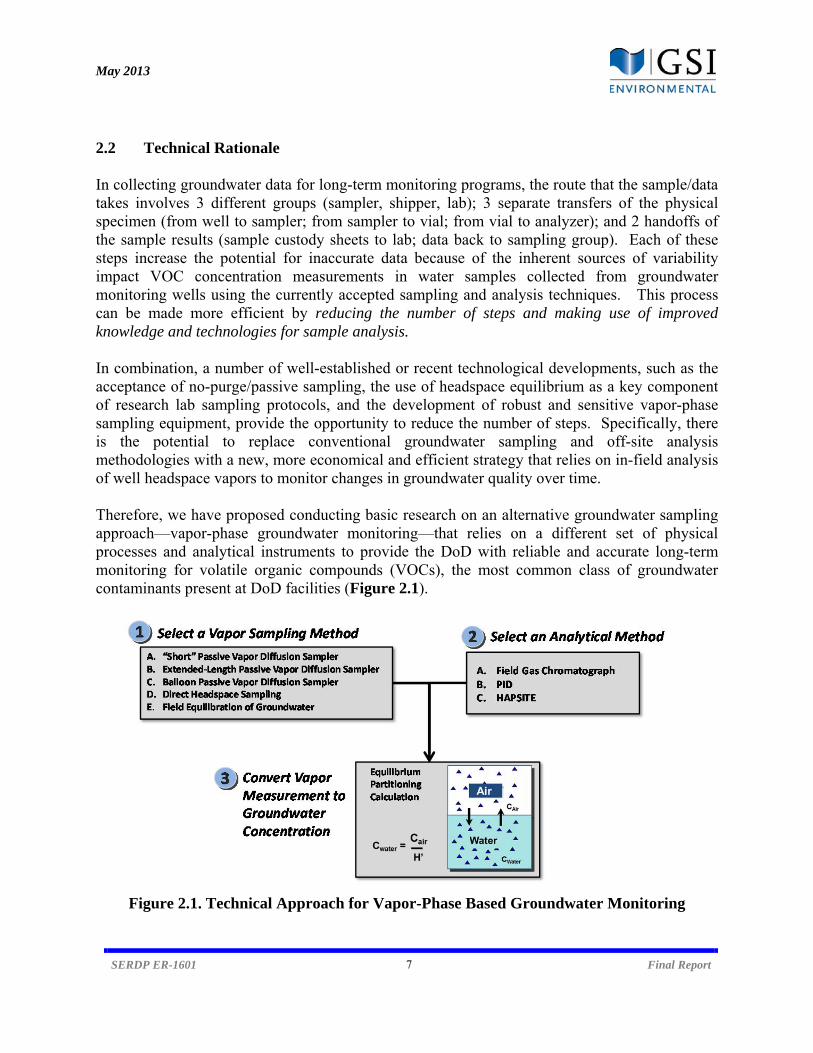
2.2 Technical Rationale In collecting groundwater data for long-term monitoring programs, the route that the sample/data takes involves 3 different groups (sampler, shipper, lab); 3 separate transfers of the physical specimen (from well to sampler; from sampler to vial; from vial to analyzer); and 2 handoffs of the sample results (sample custody sheets to lab; data back to sampling group). Each of these steps increase the potential for inaccurate data because of the inherent sources of variability impact VOC concentration measurements in water samples collected from groundwater monitoring wells using the currently accepted sampling and analysis techniques. This process can be made more efficient by reducing the number of steps and making use of improved knowledge and technologies for sample analysis. In combination, a number of well-established or recent technological developments, such as the acceptance of no-purge/passive sampling, the use of headspace equilibrium as a key component of research lab sampling protocols, and the development of robust and sensitive vapor-phase sampling equipment, provide the opportunity to reduce the number of steps. Specifically, there is the potential to replace conventional groundwater sampling and off-site analysis methodologies with a new, more economical and efficient strategy that relies on in-field analysis of well headspace vapors to monitor changes in groundwater quality over time. Therefore, we have proposed conducting basic research on an alternative groundwater sampling approach—vapor-phase groundwater monitoring—that relies on a different set of physical processes and analytical instruments to provide the DoD with reliable and accurate long-term monitoring for volatile organic compounds (VOCs), the most common class of groundwater contaminants present at DoD facilities (Figure 2.1).
Figure 2.1. Technical Approach for Vapor-Phase Based Groundwater Monitoring
May 2013
SERDP ER-1601 8 Final Report
A key part of our original hypothesis was that in-well mixing will support equilibrium partitioning between the water and air phases in the monitoring well. For cases where this is true, in-field vapor-phase monitoring of well headspace samples will provide an accurate measurement of VOC concentrations within groundwater at these monitoring wells. Conventional groundwater sampling historically involved purging a large volume of water from the monitoring well prior to sample collection in order to ensure that VOC concentrations in the water sample were representative of aquifer conditions. However, an improved understanding of both aquifer and well dynamics has led to several important shifts in the way groundwater sampling is now performed. First, low-flow purging at rates which prevent drawdown became accepted as a way to ensure that water being sampled was more representative of water in the adjacent formation. Low-flow sampling is now the sampling method of choice at most sites (Barcelona et al., 2005). Second, there is growing recognition that VOC concentrations in the aquifer can be more variable and stratified than previously thought. A large number of studies have demonstrated that VOC concentrations in groundwater can vary by orders-of-magnitude over short vertical distances (e.g., Church and Granato, 1996; Powell and Puls, 1993; Martin-Hayden, 2000; Martin-Hayden and Wolfe, 2000; Guilbeault et al., 2005). Because of aquifer heterogeneity, it is perhaps unrealistic to expect a single water sample to provide a comprehensive characterization of concentrations in the aquifer in the immediate vicinity of the well. Instead, samples from monitoring wells via pumping typically provide an approximately flow-weighted average measurement from the portion of the aquifer screened by the well, even when low-flow purging is employed (Martin-Hayden et al., 1991; Hutchins and Acree, 2000; McDonald and Smith, 2009). There is a push towards using shorter screened intervals to generate higher-resolution data that better delineates contaminant stratification, but it is our experience that long (10-ft) screens are still (by far) the most commonly implemented screen length for monitoring well. Further, studies of in-well groundwater flow indicate that ambient well bore mixing of groundwater within a monitoring well can strongly influence monitoring results (e.g.; Martin-Hayden, 2000; Elci, 2001). Vertical ambient flow within a well would mask any heterogeneity in contaminant concentrations. However, it would minimize the need for purging prior to collection of water samples because similar concentrations could be expected regardless of the vertical locations where the samples were collected. Work by Church and Granato (1996), Elci (2001), Britt (2005), and others suggest that vertical flow and in-well mixing occur in a large percentage of all monitoring wells, and may be induced even during low-flow purging. This understanding of well dynamics is consistent with the finding that low-flow purge sampling methods (Barcelona et al., 2005) and no-purge sample collection methods (e.g., Vroblesky, 2001) tend to yield results comparable to traditional high-volume purge methods. Because of this mixing, no-purge methods are gaining increasing acceptance over time (Newell et al., 2000; ITRC, 2004; Verreydt, 2010; Britt et al., 2010).
May 2013
SERDP ER-1601 9 Final Report
Several researchers have started to examine the influence of these well dynamics factors on monitoring results, with a focus on the impact of vertical flow caused by density or head difference within the monitoring well. Martin-Hayden (2000b) found that in-well flow dynamics associated with extremely small density gradients (associated with either temperature gradients or solute concentration gradients) could alter the flow induced by low-flow purging and can thereby change the sample results. Vroblesky et al. (2006, 2007) demonstrated that vertical temperature gradients could result in convective transport of dissolved oxygen from the atmosphere inside the screened interval of the well during thermally unstable conditions, but this convective process did not occur during thermally stable conditions. Mayo (2010) showed in wells screened across a heterogeneous formation, head differences as small as 0.01 m could cause well bore mixing that resulted in significant vertical redistribution of contaminants. Regardless of their origin, these gradients can influence the degree to which concentrations estimated using vapor samples from various locations in a monitoring well can be correlated to groundwater concentrations. For example, the potential for seasonally-changing stable or unstable conditions based on temperature gradients should be a factor when selecting appropriate sampling dates. The growing acceptance of no purge and passive sampling methods is consistent with the position that water within the well bore is largely representative of aquifer water (or alternatively, that quantifying this difference may not be relevant for site-specific monitoring objectives). Enhanced understanding how contaminant concentrations measured in a well using passive sampling devices (or in-situ sensors) relate to contaminant concentrations in the surrounding formation is a focus of another on-going SERDP project (ER-1704). In cases where there is little vertical stratification, or where this stratification is eliminated through ambient vertical flow within the borehole, there should be minimal difference between data collected either low-flow and no-purge methods. Consequently, a vapor-phase measurement of this well water may also be representative of concentrations in groundwater. Assuming equilibrium partitioning occurs, this sample can be collected from the well headspace. It should be clear that passive methods—including those based on vapor analysis—would not be able identify stratification in wells where vertical flow was present (Metcalf and Robins, 2007; MacDonald and Smith, 2009). For those wells installed in formations with significant vertical stratification and there is poor in-well mixing, a vapor sample from the well headspace may not be representative of groundwater concentrations. If a correlation is to be attempted in these cases, attention must be paid to the vertical location where the corresponding groundwater sample is collected. For a low-flow groundwater sample that is typically (but not always) collected near the center of the well screen, a vapor sample from the same vertical location would likely yield more comparable results. In these cases, passive methods for collecting vapor samples—such as the use of a semi-permeable bag submerged in the water column—may be a better option for determining the groundwater concentration. However, the degree of mixing induced even by low-flow purging may result in differences with data collected using passive methods. As a result, in wells with significant stratification (and minimal vertical flow), the concentrations obtained using passive samplers are
May 2013
SERDP ER-1601 10 Final Report
likely to be more representative of the depth at which they are employed (Divine et al., 2005). For multi-level sampling, this means that passive sampling methods should be an improvement over low-flow purging methods. This discussion is consistent with the increasing realization in the environmental community that when designing a monitoring program, it is important to have an understanding of what type of data will be generated by the chosen sampling and analysis method. In developing alternative monitoring strategies, the data are generally compared to current methods, and low flow groundwater data are the typical baseline due to widespread use (Divine et al., 2005). Comparisons with low-flow groundwater data were used extensively for these comparative purposes during the current project, but with the realization that low-flow groundwater data are not necessarily the most representative of formation conditions in all cases. Understanding the sources of variability (and methods for mitigating that variability) in groundwater monitoring data are the focus of several other DoD-sponsored efforts (e.g., SERDP ER-1705) 2.3 Monitoring Approaches Tested During Laboratory Validation Study 2.3.1 Vapor-Phase Monitoring Equipment To collect vapor-phase samples, there are a variety of commercially-available vapor monitoring equipment that are field-ready and highly functional. Recent advances have resulted in instruments capable of detecting and quantifying gas-phase VOCs in the low ppbv concentration range. These instruments are commonly used for exposure monitoring in industrial and environmental clean-up settings. However, several devices have potential utility in monitoring VOCs in water, and have been successfully tested as part of the U.S. EPA’s Environmental Technology Verification Program through the Advanced Monitoring Systems Center (USEPA, 2012) (http://www.epa.gov/nrmrl/std/etv/vt-ams.html#wmtfmoc). An objective of the laboratory-based study will be to verify that these instruments can be used to accurately determine the VOC concentration in water samples through the measurement of VOC concentration in head space vapors in equilibrium with the water samples. Consequently, validation within the laboratory study is necessary prior to the start of a larger field demonstration program. Field instruments that are available range from those that are intended for simple screening-level investigations to more expensive devices that are capable of definitively identifying and measuring concentrations in the part-per-trillion range. While the latter may be equipped with advanced detection capabilities (such as GC/MS) and data processing methods, they require a higher level of training to use and to interpret results. Typically, simpler vapor instruments known generically as portable vapor analyzers (PVAs) are used for general surveying and site investigation, when identification of specific compounds is unnecessary. These devices are often labeled as a “PID” (photoionization detector), even if the device is equipped with some other type of general-purpose detector.
May 2013
SERDP ER-1601 11 Final Report
The laboratory study for the current project evaluated the accuracy, precision, and sensitivity of two types of instruments: i) a PID, specifically the “ppbRAE” from RAE Systems; and ii) a portable GC, specifically the Voyager Portable GC from Photovac. These two types of instruments were selected based on a combination of functionality (i.e., their appropriateness for measuring desired vapor-phase concentrations) and cost. A typical PID is small, relatively cheap (< $10,000), and easy to use. These devices are often capable of measuring total VOC concentrations as low as 1 ppbv but do not have the ability to differentiate between individual compounds. Consequently, the PID is likely limited to sites where single compounds are present or where knowledge of bulk concentration is sufficient. In addition, the PID requires a higher volume per sample analyzed. The portable GC is larger and has a higher cost (approximately $30,000), but it does have the capability of identifying and quantifying the contribution from individual compounds within a mixture. Manufacturers report detection limits as low as 6 ppbv for compounds such as TCE. Under equilibrium conditions, this sensitivity corresponds to TCE concentrations in water of 0.2 g/L or less. The portable GC selected for this project has both PID and ECD (electron capture detector) for measuring a wide range of contaminants (e.g., chlorinated ethenes, chlorinated ethanes, hydrocarbons). The results of a laboratory evaluation of instrument performance (submitted as part of the Interim Report in August 2009) showed that the GC and PID achieved the project criteria for accuracy, precision, and sensitivity. The ppbRAE 3000 PID achieved the accuracy and precision criteria for 100% of measurements. The instrument method detection limit (MDL) corresponds to a water-phase concentration of 1.3 g/L benzene, less than the MCL of 5 g/L. The Voyager GCs achieved the accuracy criteria for 94% of measurements and the precision criteria for 100%. For each of the three VOCs, the instrument MDL corresponds to a water-phase concentration of less than 0.5 g/L, less than the MCL of 5 to 7 g/L. Based on these findings, we recommend that both instruments be retained for the field portion of the study. 2.3.2 Vapor-Phase Sampling Methods In addition to relying on the performance of these field instruments, the utility of the proposed monitoring approach is a function of the degree of equilibrium partitioning that takes place (i.e., the method by which a vapor sample can be correlated to a liquid sample) and the ability to collect a representative vapor sample from a monitoring well (i.e., the sampling technique). Both of these latter components are important parts of the validation procedure. As part of the laboratory study, a method validation was completed using a series of bench-top reactors to determine if headspace equilibration provides an accurate method for determining the corresponding aqueous-phase concentration. At least three different types of sampling methods
May 2013
SERDP ER-1601 12 Final Report
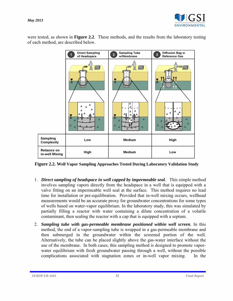
were tested, as shown in Figure 2.2. These methods, and the results from the laboratory testing of each method, are described below.
Figure 2.2. Well Vapor Sampling Approaches Tested During Laboratory Validation Study
1. Direct sampling of headspace in well capped by impermeable seal. This simple method involves sampling vapors directly from the headspace in a well that is equipped with a valve fitting on an impermeable well seal at the surface. This method requires no lead time for installation or pre-equilibration. Provided that in-well mixing occurs, wellhead measurements would be an accurate proxy for groundwater concentrations for some types of wells based on water-vapor equilibrium. In the laboratory study, this was simulated by partially filling a reactor with water containing a dilute concentration of a volatile contaminant, then sealing the reactor with a cap that is equipped with a septum.
2. Sampling tube with gas-permeable membrane positioned within well screen. In this method, the end of a vapor-sampling tube is wrapped in a gas-permeable membrane and then submerged in the groundwater within the screened portion of the well. Alternatively, the tube can be placed slightly above the gas-water interface without the use of the membrane. In both cases, this sampling method is designed to promote vapor-water equilibrium with fresh groundwater passing through a well, without the possible complications associated with stagnation zones or in-well vapor mixing. In the
May 2013
SERDP ER-1601 13 Final Report
laboratory study, this is simulated by placing a long tube in sealed reactor that is partially filled with water containing a dilute concentration of water, and then sampling from this tube. Following equilibration, samples are collected from the tubes, with the lab study focusing on the importance of purging and diffusion rates in collecting a representative sample.
3. Diffusion sampler filled with reference gas. This approach is very similar to existing diffusion bags, which are submerged in the groundwater in the screened portion of the well, except that, in this case, the diffusion bag would be filled with a reference gas (air) rather than a liquid. This method for collecting vapors in equilibrium with water has been described previously for quantifying dissolved gases (Sanford et al., 1996; Spalding and Watson, 2006, 2008; MacLeish et al., 2007; Gardner and Solomon, 2009) and volatile contaminants in soil gas (Kerfoot and Mayer, 1986), sediment pore water (Vroblesky et al., 1996; Vroblesky and Campbell, 2001; USGS, 2002), and lab-scale systems (Divine and McCray, 2004). However, they are largely untested in groundwater monitoring wells. In several USGS-led studies (2002), the samplers consisted of 40-mL sampling vials wrapped in layers of gas-permeable membrane. The lab study (and all of the field studies) that were completed as part of the current project utilized the same USGS-based configuration in constructing the passive vapor diffusion (PVD) samplers. These samplers are submerged in water within sealed reactors and contaminants diffuse across the plastic membrane based on the concentration gradient. They are allowed to equilibrate prior to removal, a process that typically takes days to several weeks (although more precise predictions on equilibration times are presented in Sanford et al., 1996 and Divine and McCray, 2004 using calculation based on Fick’s law of diffusion). Vapors from the equilibrated samplers can then be analyzed. In the field, this approach is slightly more complicated than the other methods because the diffusion sampler must be removed from the well for analysis. However, this approach maximizes the potential for attainment of equilibrium between the water and vapor phases and minimizes number of variables that could affect the correlation of VOC concentration in the vapor phase to that of the groundwater phase.
2.4 Monitoring Approaches for Field Testing 2.4.1 Vapor-Phase Sampling Methods The design of the field programs—which are described in detail in Section 3—was intended to test the importance of field factors that could not easily be simulated in a laboratory setting (i.e., monitoring wells with long-screens and ambient flow). The following techniques were included in the various field programs:
Direct Headspace Sampling: This method relies on sampling vapors directly from the headspace in a well that is equipped with a valve fitting on an impermeable well seal at the surface. Conventional compression-type screw-caps are suitable for this method,
May 2013
SERDP ER-1601 14 Final Report
with the primary modification being the installation of a valve and sampling line that can be connected to a sampling syringe. The well headspace sample can be collected with a small-volume, gas-tight syringe (< 1 mL) and injected directly into the field-portable GC. Alternatively, the well headspace sample can be collected with a larger syringe (> 15 mL) and then transferred to a Tedlar bag. Samples from the bag are then injected to the field-portable GC or direct to the influent line of the PID. Note that direct headspace sampling is the simplest method and requires no lead time for installation or pre-equilibration.
Passive Vapor Diffusion (PVD) Sampling: PVD samplers are gas-filled containers submerged in the water column that can be used for monitoring the concentration of water in equilibration with a gas phase. By incorporating a semi-permeable membrane into the design, these devices permit diffusion of VOC vapors across the membrane and into the samplers while preventing water from entering the vials. The PVD sampler design included in most of the field programs in the current study is identical to that used by the USGS during previous validation studies (USGS, 2002) for sediment sampling. Specifically, the samplers consist of a 40-mL VOA glass vial sealed in two layers of gas-permeable LDPE tubing. Alternative designs that were also tested were based on longer samplers (2.5 to 5-ft) that provided more cross-sectional area for diffusion and covered a greater portion of the screened interval (Note that increasing the area-to-volume ratio decreases the required equilibration time). PVD samplers can be positioned in the wells by affixing them to support tubing with self-locking nylon ties or string. The tubing or string extends from the wellhead caps at a length to allow for complete submersion of the samplers at the midpoint of the screened interval of the well. Weights attached to the base of the samplers are used to overcome buoyancy within the well.
In the field, this approach is slightly more complicated than direct headspace sampling because the diffusion sampler must be (i) installed in advance to allow for equilibrium conditions to be attained (approximately 2 to 3 weeks based on the lab validation study and USGS guidance; additional guidance on site-specific equilibration times can be found in Devine and McCray, 2004)); and (ii) removed from the well for analysis, such that disturbance of equilibrium conditions may influence subsequent samples collected during the same monitoring event (Divine and McCray, 2004). Further, the concentration result is time-integrated average due to the extended deployment periods (Divine and McCray, 2004). However, this approach maximizes the potential for attainment of equilibrium between the water and vapor phases and minimizes number of variables that could affect the correlation of VOC concentration in the vapor phase to that of the groundwater phase. Furthermore, methods for installing samplers are similar to those for the passive water diffusion bag, and results from the PVD sampler can be compared directly to those obtained using the passive water diffusion bag for further validation. A key consideration when using passive vapor diffusion samplers is the impact of pressure within the monitoring well on the concentration estimated using on-site vapor-phase analysis. For example, samplers installed within monitoring wells where there is a
May 2013
SERDP ER-1601 15 Final Report
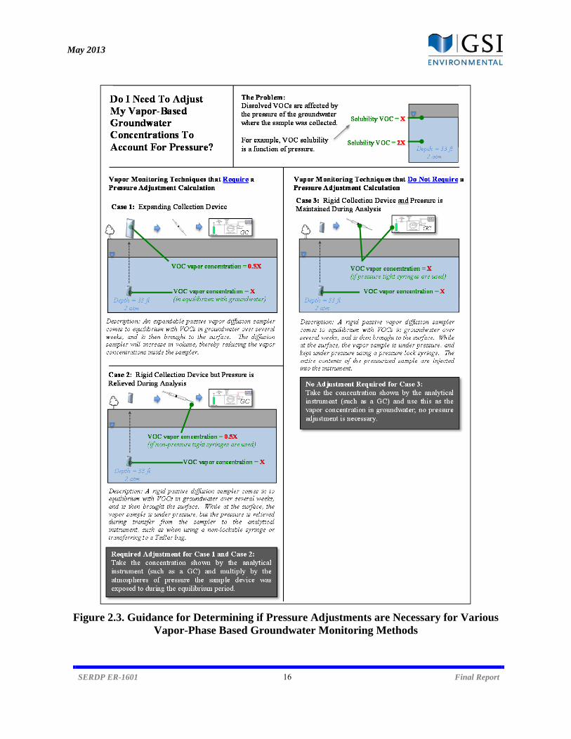
thick water column above the sampler can be subject to considerable hydrostatic pressure during the equilibrium process. The sampler design and analytical procedure can dictate whether that in situ pressure is maintained or relieved prior to sample analysis. If pressure is not maintained, then a pressure adjustment is necessary to convert the vapor-phase concentration to an equivalent groundwater concentration. Guidance for determining whether pressure adjustments are necessary is provided in Figure 2.3 on the following page, while the correction procedure is detailed in Section 3.4.1.
May 2013
SERDP ER-1601 16 Final Report
Figure 2.3. Guidance for Determining if Pressure Adjustments are Necessary for Various Vapor-Phase Based Groundwater Monitoring Methods
May 2013
SERDP ER-1601 17 Final Report
2.4.2 Water-Phase Sampling Methods Comparisons of vapor-based sampling methods to more conventional groundwater monitoring methods are an important part of the field programs. There are two primary methods for collecting groundwater samples that were judged suitable for comparison:
Low-Flow Sampling: Low-flow sampling is a low stress method of purging and sampling a monitoring well that has gained widespread regulatory acceptance over the past 15 years. Standard practices for conducting low-flow sampling are outlined in ASTM D 6771 (2002), and further information is provided in multiple guidance documents published by federal agencies (e.g., Puls and Barcelona, 1996). The key procedure involves pumping small volumes of groundwater from the well screen at flow rates (typically 100 to 500 mL/min) that prevent drawdown. This is intended to minimize i) the disturbance of potentially-stagnant water from above or below the well screen; ii) the movement of groundwater from the formation to the well that is normally induced by high volume purging; and iii) the amount of purge water that must be handled as waste. As a result, the groundwater sampled during low-flow purging is thought to be more representative of the groundwater adjacent to the screen. Samples are collected using either pumps placed at the well screen, or surface pumps (e.g., peristaltic) with an intake line that terminates at the center of the screen. Pumping continues until stabilization of specific geochemical parameters (e.g., pH, conductivity) is attained, and samples are transferred to 40-mL VOA vials suitable for lab analysis.
For this project, samples were typically collected using peristaltic pumps, which represent an accepted low-flow technique but, like many pumping techniques, can result in slight low bias when collecting gas-charged groundwater samples (Barker and Dickhout, 1988; Parker, 1994; MacLeish et al., 2007). This is due to degassing that occurs when a pressurized sample (i.e., under hydrostatic pressure within a well) is brought to the surface, particularly with a suction lift techniques employed by a peristaltic pump where a vacuum is imposed on the sample (Barker and Dickhout, 1988). The result is that dissolved gases are stripped via effervescence (Roy and Ryan, 2010), contributing to losses of any VOCs in the water This process has been reported to decrease the VOC concentration in the water by varying degrees. Barker and Dickhout (1988) reported losses of 9 to 33% using peristaltic pumps. Regardless of the low-flow sampling method, the exact amount of VOC loss is site-specific because it is highly dependent on the level of gas saturation (total dissolved gas pressure), which is a function of the depth of the water column and the groundwater geochemistry.
Field Equilibration of Vapor from Low-Flow Samples: An alternative to direct analysis of the water collected during low-flow sampling involves field analysis of the vapor in equilibration with the same low-flow groundwater sample. The water is collected identically but the sampling container (e.g., 40-mL vial) is only partially filled instead of completely. After sealing the container, shaking, and allowing for suitable equilibration (minutes to hours depending on the compound and level of mixing), the headspace vapor

May 2013
SERDP ER-1601 18 Final Report
is then analyzed on-site using appropriate field equipment. While this method requires collection (and disposal) of groundwater, it has the advantage that the VOC concentration is estimated based on water that is identical to the low-flow groundwater sample (and presumably equally representative of the groundwater adjacent to the screen). Similar methodology (headspace equilibration of groundwater) is used for other common environmental analyses (e.g., dissolved gases via RSK-175, Kampbell and Vandegrift, 1998). The primary difference is that the equilibration and analysis is done in the field with partially-filled containers instead of displacement of liquid volume and subsequent headspace analysis at a fixed lab.
Passive Diffusion Bags: Passive diffusion samplers is a term used to describe a number of different “no-purge” sampling techniques that rely on diffusion of groundwater contaminants across a semi-permeable membrane to permit equilibration between water within the sampling device and surrounding groundwater. A full description of a number of many commercially-available devices and protocols for their use are outlined in a series of recently-published guidance documents (e.g., ITRC, 2004, 2006, 2007). This guidance has facilitated their regulatory acceptance, although their use in long-term monitoring programs is typically approved on a case-by-case basis (ITRC, 2007). Passive/no-purge sampling methods described in these documents and/or otherwise in development include the Snap sampler (from ProHydro Inc.), HydraSleeve (from GeoInsight), the Gore Module (from W.L. Gore), and the IS2 method (being tested as part of ESTCP ER-201122). The most commonly-used are passive diffusion bags (PDBs) that generally consist of a rigid or collapsible “bag” that is filled with water and then deployed within the well for several weeks to allow for diffusion across the gas-permeable bag. The required duration to ensure equilibration varies due to site-specific and compound-specific factors but a minimum of two weeks is generally recommended (ITRC, 2004). In practice, this duration matters little because the devices are often installed for several months, i.e., between quarterly monitoring events. Following retrieval, groundwater from the passive samplers can be transferred to method-appropriate vials and sent for lab analysis. The resulting groundwater concentration represents a time-averaged concentration during the period of deployment, with the understanding that results are generally biased towards the latter deployment period. As with low-flow sampling, a key advantage of passive sampling relative to high-volume purging is that minimal or no waste is generated. While passive devices are often installed at the well screen to provide results comparable to low-flow sampling, they are ideally suited for sampling discrete intervals within the well. Consequently, they can be used in locations where vertical stratification within the water-bearing unit is suspected.
The inclusion of passive water sampling methods within the current field study provided a means for comparing depth-discrete sampling data collected by different analytical techniques (i.e., vapor analysis vs. water analysis) and passive vs. low-flow methods.
May 2013
SERDP ER-1601 19 Final Report
2.5 Potential Influence of Temperature Gradients on Monitoring
Vertical temperature gradients are created in shallow soils (i.e., <15 m) due to seasonal changes in air temperature and solar radiation (Wu and Nofziger, 1999). As the surface soil warms and cools, the change in temperature propagates downward by thermal diffusion. As a result, temperatures in shallow soils generally decrease with depth in late summer and increase with depth in late winter. During other times of the year, mixed temperature profiles exist with very shallow soils reflecting recent changes in surface soil temperature and deeper soils reflecting temperature gradients associated with the prior season Accurate predictions of the vertical temperature profile over time in shallow soil can be made based on a knowledge of soil clay content, soil water content, and maximum and minimum seasonal surface soil temperature (Wu and Nofziger, 1999). Clay content and water content affect thermal diffusivity, which in turn affects the shape of the vertical temperature profile. The difference between maximum and minimum seasonal soil temperature defines the magnitude of the temperature gradient, but does not affect the shape of the profile. Because the density of water changes with temperature, a vertical temperature gradient yields a corresponding vertical density gradient. When groundwater temperature increases with depth, the density decreases with depth and vice versa. Temperature gradients of less than 0.01°C per meter (0.003°C per foot) that increase with depth are sufficient to support thermal convection resulting in mixing between depths within monitoring wells (Sammel, 1968); however significantly higher temperature gradients are needed to induce vertical flow within the aquifer formation due to the flow resistance associated with the porous medium. As a result, vertical temperature gradients that do not affect the vertical flow within an aquifer can have a dramatic effect on the flow dynamics and mixing of dissolved contaminants within a monitoring well. Specifically, increasing temperature with depth below ground surface causes thermally unstable conditions and promotes convective mixing within the well. Decreasing temperatures, on the other hand, cause thermally stable conditions that serve to inhibit mixing and may counteract other forces that would normally result in mixing. Within shallow aquifers (i.e., <15 m bgs), the magnitude and direction of the vertical temperature gradient change from season to season.
• Late winter: Formation temperatures generally increase with depth causing thermally mixed conditions within the well;
• Late summer: Formation temperatures generally decrease with depth causing thermally stabilized conditions within the well;
• Other times of the year: Formation temperatures may increase with depth over one portion of the well (for example the upper half) and increase with depth over another portion (for example the lower half), resulting in a complex pattern of temperature induced mixing and stratification.
May 2013
SERDP ER-1601 20 Final Report
With traditional high-volume sampling methods that were widely employed in the 1980s and early 1990s, vertical temperature gradients likely had a minimal impact on sampling results. Traditional sampling methods require removal of at least three casing volumes of water from a well prior to sampling. The commonly used methods for purging this water from the well (e.g., bailer, Waterra pump, downhole pump operated at high flowrates) result in significant mixing of the water within the well. For example, pumping a 2-inch monitoring well at 3 gallons per minute (gpm) results in a Reynolds number of 4850, which is well within the turbulent region for moving water. As a result, any stratification that occurred under ambient flow conditions was most likely disrupted prior to sample collection. However, the now widely-accepted low-flow and no-purge sampling methods appear to be extremely vulnerable to mixing effects from seasonal changes in temperature gradients, and these effects may significantly impact sample results. This can be visualized by recognizing that one goal of low-flow and no-purge sampling methods is to avoid turbulent conditions during sample collection (ASTM, 2002; Vroblesky, 2001). For example, pumping a 2-inch monitoring well at a commonly-used low-flow rate of 400 mL per minute (or ~0.1 gpm) results in a Reynolds number of 170, which is well within the laminar region for moving water. By maintaining laminar flow conditions during purging and sample collection, the sampling process does not mobilize sediment from the bottom of the well or stagnant water present above the screened interval. For the same reason, low-flow and no-purge sampling methods maintain laminar flow conditions and are unlikely to disrupt the naturally-occurring ambient flow conditions created by the presence of vertical temperature gradients in many wells. In the absence of hydraulically-induced or solute-induced vertical pressure gradients (i.e., gradients associated with recharge conditions or other non-temperature vertical gradients) within the portion of the aquifer penetrated by a monitoring well, flow within a shallow monitoring well is likely to be most strongly influenced by the vertical temperature gradient.
• In late winter, when increasing temperature with depth results in convective mixing, water within the screened interval of the well is likely to be well mixed. As a result, samples collected by either low-flow or no- purge sampling methods will reflect a flow-weighted average of the contaminant concentrations within the screened portion of the aquifer. Under these conditions, any sample collected from any portion of the screened interval by a low-flow or no purge sampling method will yield this flow-weighted average concentration.
• In late summer, when decreasing temperature with depth inhibits mixing, contaminant concentrations at a specific depth within the screened interval will be representative of the contaminant concentrations within the aquifer at this depth. If contaminant concentrations in the aquifer are highly stratified, then these stratified conditions will also be present within the well. Under these conditions, the contaminant concentrations measured using either low-flow or no-purge sampling methods will be highly dependent on the exact vertical location of sample collection device intake, where even a few tens of centimeters can result in orders-of-magnitude changes in concentration.
May 2013
SERDP ER-1601 21 Final Report
As a result of these seasonally changing temperature gradients, the water sample collected using low flow and no purge sampling methods can yield very different results at different times of year for shallow monitoring wells even if the sampling is conducted in a highly reproducible manner (i.e., consistent sample depth and purge volume).

May 2013
SERDP ER-1601 22 Final Report
3. MATERIALS AND METHODS
The program described herein consisted of the collection of a series of vapor and groundwater samples from a lab-scale reactors or existing monitoring wells, followed by analyses of data to establish relevant correlations between each of the sampling and analysis methods. A brief summary of the project tasks described in this report are provided below.
1. Laboratory Validation of Vapor-Phase Monitoring: Two portable field instruments (PID and portable GC) were tested under controlled conditions to assess accuracy, precision, and sensitivity. In addition, validation of three methods for collecting headspace vapor samples and correlating the resulting vapor concentrations to groundwater concentrations was performed.
2. Temperature Study: Because the accuracy of vapor-phase monitoring of a monitoring well sampling relies on equilibration of VOCs between groundwater and the well headspace, the study was designed to test the hypothesis that temperature-driven density gradients in monitoring wells may have a seasonal impact on in-well mixing.
3. Preliminary Field Study: The goal of the initial phase of field testing was to assess the performance of the field-portable instruments and several proposed sample collection methods under real field conditions. For this task, data collected using vapor-phase based methods were evaluated in terms of accuracy relative to more conventional groundwater sampling and analyses methods.
4. Expanded Field Study: Several modifications of the passive sampling methods identified as promising during the preliminary phase of field testing were further examined in a larger-scale study, with additional field equipment (HAPSITE) included to demonstrate potential advantages.
5. Supplemental Field Testing: A longer-term field program was implemented to assess the amount of event-to-event or site-to-site variability associated with the most promising vapor-phase based methods. In addition, the impact of various groundwater collection methods was tested to determine if these methods reduce the variability in vapor and/or groundwater concentrations and improved correlations.
6. Assessment of Cost-Effectiveness: Direct comparisons between monitoring alternatives were evaluated based on “cost per sample” and other applicable metrics. This includes a the development of an appropriate cost model and projection of costs over the lifetime of a sampling program, including any potential cost savings that could be reasonably anticipated based on scale-up costs, local subcontractors, or other factors.
The report is organized such that methods and results for each of the tasks are described in separate sections, with the understanding that early results were used to refine the experimental design of subsequent tasks. The collective results were used to develop the User’s Manual for vapor-based groundwater monitoring methods that is Appendix C of this report.
May 2013
SERDP ER-1601 23 Final Report
Further, the objectives of this project also evolved over the course of the project based on findings during the early stages. Significant modifications include i) the addition of a study on the potential effects of temperature on in-well mixing and relationships between vapor and groundwater concentration in a monitoring well; and ii) performing several smaller-scale field programs in lieu of one larger-scale program. Also, one of the original project objectives was to identify aquifer and well conditions that contributed to sampling variability when applying these methods. While this objective was still a component of the current study, the bulk of the work to address this objective is being completed as part of a parallel project (SERDP ER-1705) that has a broader goal of understanding variability in all groundwater monitoring programs. 3.1 Laboratory Validation Study The laboratory validation study consisted of: 1) validation of two portable field instruments (PID and portable GC), 2) validation of headspace analysis as a method to measure the concentration of a VOC in water, and 3) validation of the three methods for collection of headspace vapor samples. Two types of field instruments were been selected for this phase of the project:
1. Gas Chromatograph (GC): Voyager (Photovac, Inc.) equipped with a 10.6 eV photoionization lamp detector and an electron capture detector (ECD).
2. Photoionization Detector (PID): ppbRAE 3000 (RAE Systems Inc.) equipped with a 10.6 eV photoionization lamp detector.
Three VOCs, 1,1-dichloroethene (1,1-DCE), benzene, and trichloroethene (TCE), were selected for the laboratory validation study based on: i) the availability of pure and gas-phase standards for these VOCs; ii) the common occurrence of these VOCs as groundwater contaminants at DoD facilities; and iii) the low MCLs for these VOCs in drinking water (i.e., 5 g/L for TCE and benzene, 7 g/L for 1,1-DCE). Other common volatile groundwater contaminants (e.g., tetrachloroethene, vinyl chloride, etc.) have similar chemical properties and would be expected to yield similar laboratory validation results. For the laboratory validation study, we evaluated the accuracy, precision, and sensitivity of the field instruments and headspace analysis method, and the accuracy and precision of the three sample collection methods. The quantitative objectives for accuracy and precision are based on standard environmental data quality objectives.
Accuracy: the agreement between a measured value and a known value. The accuracy objective was a relative percent difference (RPD) of +/- 30% between the measured and known values for 75% of measurements.

May 2013
SERDP ER-1601 24 Final Report
Precision: the agreement between replicate measured values. The precision objective was a relative standard deviation (RSD) for the replicate sample set of 30% for 75% of measurements.
Sensitivity: the lowest concentration at which accuracy and precision goals can be achieved. The two primary sensitivity objectives included i) Instrument MDLs less than the federal drinking water standard (i.e., the MCL - 5 g/L for many VOCs; and ii) attainment of accuracy and precision goals at VOC concentrations in water less than MCLs.
3.1.1 Portable Field Instrument Validation Single VOC and mixed VOC standard gases were used for the instrument validation. The gases were: benzene at 1.04 ppm (Scott Specialty Gases) and 5 ppm (Spec Air Specialty Gases), and an equal mixture of 1,1-dichloroethene (1,1-DCE), benzene, and trichloroethene (TCE) at 0.33 ppm, 3.06 ppm, and 31.20 ppm total concentrations (Spectra Gases). During the laboratory study, the instruments were calibrated according to manufacturers’ protocols. Isobutylene was used as the calibration standard for the PID. The standard gas mixtures were used for 3-point calibrations of the Voyager GCs. Following calibration, the accuracy, precision, and sensitivity of each instrument was determined using the standard gases and operating the instruments in accordance with the manufacturers’ instructions. Two of the same model of Voyager GC were tested.
Figure 3.1. Portable field instruments used for the detection of vapor-phase volatile organic
compounds. (A) ppbRAE 3000 PID; and (B) Photovac Voyager GC. 3.1.2. Validation of Headspace Analysis Method Following instrument validation, the use of vapor-phase headspace analysis to determine the VOC concentration in water was validated through a series of equilibrium partitioning experiments. For each experiment, a known mass of one or more VOCs was added to a vial partially filled with water and also containing air-phase headspace. Immediately after the
May 2013
SERDP ER-1601 25 Final Report
addition of the stock VOC solution the vials were shaken briefly to ensure uniform distribution of the VOCs in the aqueous phase and then left undisturbed for the duration of the experiment. An initial experiment was conducted to determine the time required to ensure equilibrium partitioning between the water and air phases, and this time was used as the minimum equilibration time for the remaining experiments. Following equilibration, the VOC concentration in the headspace was measured using the field GC operated in accordance with manufacturers’ instructions. The measured headspace VOC concentration was used to calculate a “measured” VOC concentration in water based on Henry’s law equilibrium partitioning relationship:
'H
CC a
w
Where Cw = VOC concentration in water (μg/L), Ca = VOC concentration in air ( converted to μg/L), and H’ = Dimensionless Henry’s law constant Henry’s law constants were adjusted for temperature as follows:
293
11
20,
' 10 TB
CccHH
Where Hcc,20°C is the Henry’s constant at 20°C (9.75 x 10⁻¹ for 1,1-DCE, 1.91 x 10⁻¹ for benzene, and 3.14 x 10⁻¹ for TCE), B is a fitting parameter (1586 for 1,1-DCE, 1693 for benzene, 1871 for TCE), and T (°K) is the experimental temperature (Staudinger and Roberts, 2001). The accuracy of the method was evaluated by comparing the VOC concentration in water measured using the vapor-phase analysis to the known VOC concentration in water (calculated based on the known mass of VOC added to the vial). The precision was evaluated by comparing the VOC concentration measured by the field GC in replicate vials containing the same known VOC concentration. The use of headspace analysis to measure VOC concentrations in groundwater was validated through a series of experiments (see Table 3.1). Note that these experiments were all conducted using the field GC. The PID was not used because the bench-scale reactors contained limited headspace volumes that were not sufficient to support analysis by PID.
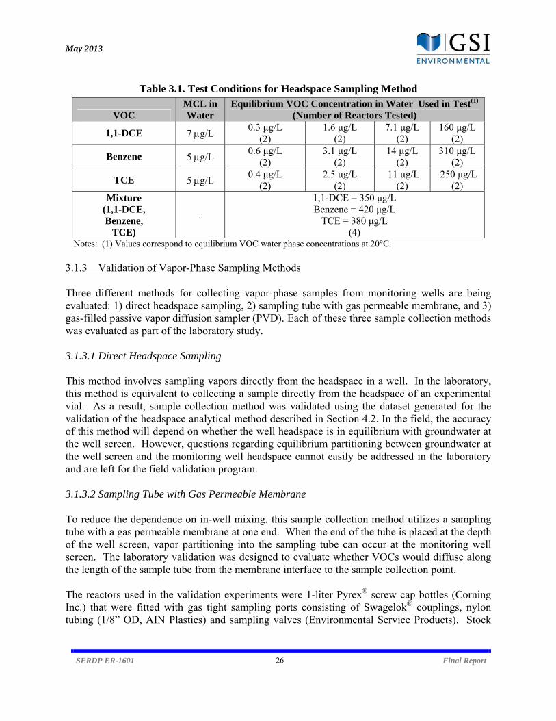
May 2013
SERDP ER-1601 26 Final Report
Table 3.1. Test Conditions for Headspace Sampling Method
VOC MCL in Water
Equilibrium VOC Concentration in Water Used in Test(1) (Number of Reactors Tested)
1,1-DCE 7 g/L 0.3 μg/L
(2) 1.6 μg/L
(2) 7.1 μg/L
(2) 160 μg/L
(2)
Benzene 5 g/L 0.6 μg/L
(2) 3.1 μg/L
(2) 14 μg/L
(2) 310 μg/L
(2)
TCE 5 g/L 0.4 μg/L
(2) 2.5 μg/L
(2) 11 μg/L
(2) 250 μg/L
(2) Mixture
(1,1-DCE, Benzene,
TCE)
-
1,1-DCE = 350 μg/L Benzene = 420 μg/L
TCE = 380 μg/L (4)
Notes: (1) Values correspond to equilibrium VOC water phase concentrations at 20°C. 3.1.3 Validation of Vapor-Phase Sampling Methods Three different methods for collecting vapor-phase samples from monitoring wells are being evaluated: 1) direct headspace sampling, 2) sampling tube with gas permeable membrane, and 3) gas-filled passive vapor diffusion sampler (PVD). Each of these three sample collection methods was evaluated as part of the laboratory study. 3.1.3.1 Direct Headspace Sampling This method involves sampling vapors directly from the headspace in a well. In the laboratory, this method is equivalent to collecting a sample directly from the headspace of an experimental vial. As a result, sample collection method was validated using the dataset generated for the validation of the headspace analytical method described in Section 4.2. In the field, the accuracy of this method will depend on whether the well headspace is in equilibrium with groundwater at the well screen. However, questions regarding equilibrium partitioning between groundwater at the well screen and the monitoring well headspace cannot easily be addressed in the laboratory and are left for the field validation program. 3.1.3.2 Sampling Tube with Gas Permeable Membrane To reduce the dependence on in-well mixing, this sample collection method utilizes a sampling tube with a gas permeable membrane at one end. When the end of the tube is placed at the depth of the well screen, vapor partitioning into the sampling tube can occur at the monitoring well screen. The laboratory validation was designed to evaluate whether VOCs would diffuse along the length of the sample tube from the membrane interface to the sample collection point. The reactors used in the validation experiments were 1-liter Pyrex® screw cap bottles (Corning Inc.) that were fitted with gas tight sampling ports consisting of Swagelok® couplings, nylon tubing (1/8” OD, AIN Plastics) and sampling valves (Environmental Service Products). Stock
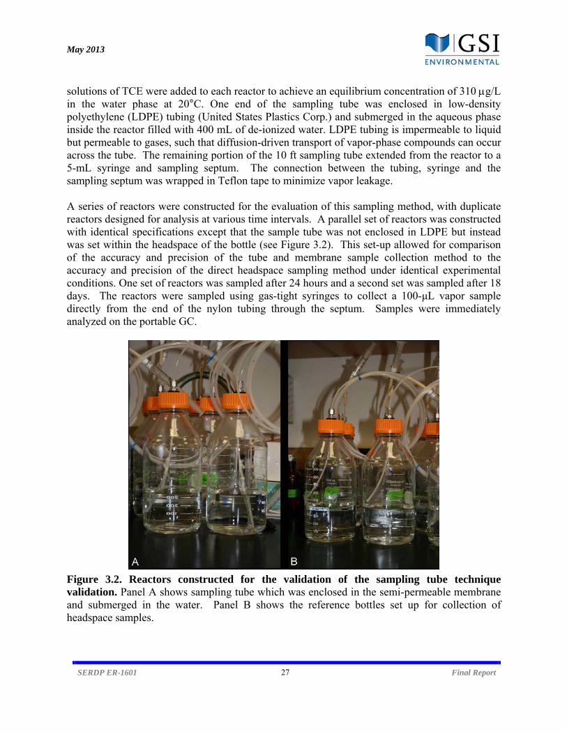
May 2013
SERDP ER-1601 27 Final Report
solutions of TCE were added to each reactor to achieve an equilibrium concentration of 310 g/L in the water phase at 20°C. One end of the sampling tube was enclosed in low-density polyethylene (LDPE) tubing (United States Plastics Corp.) and submerged in the aqueous phase inside the reactor filled with 400 mL of de-ionized water. LDPE tubing is impermeable to liquid but permeable to gases, such that diffusion-driven transport of vapor-phase compounds can occur across the tube. The remaining portion of the 10 ft sampling tube extended from the reactor to a 5-mL syringe and sampling septum. The connection between the tubing, syringe and the sampling septum was wrapped in Teflon tape to minimize vapor leakage. A series of reactors were constructed for the evaluation of this sampling method, with duplicate reactors designed for analysis at various time intervals. A parallel set of reactors was constructed with identical specifications except that the sample tube was not enclosed in LDPE but instead was set within the headspace of the bottle (see Figure 3.2). This set-up allowed for comparison of the accuracy and precision of the tube and membrane sample collection method to the accuracy and precision of the direct headspace sampling method under identical experimental conditions. One set of reactors was sampled after 24 hours and a second set was sampled after 18 days. The reactors were sampled using gas-tight syringes to collect a 100-μL vapor sample directly from the end of the nylon tubing through the septum. Samples were immediately analyzed on the portable GC.
Figure 3.2. Reactors constructed for the validation of the sampling tube technique validation. Panel A shows sampling tube which was enclosed in the semi-permeable membrane and submerged in the water. Panel B shows the reference bottles set up for collection of headspace samples.
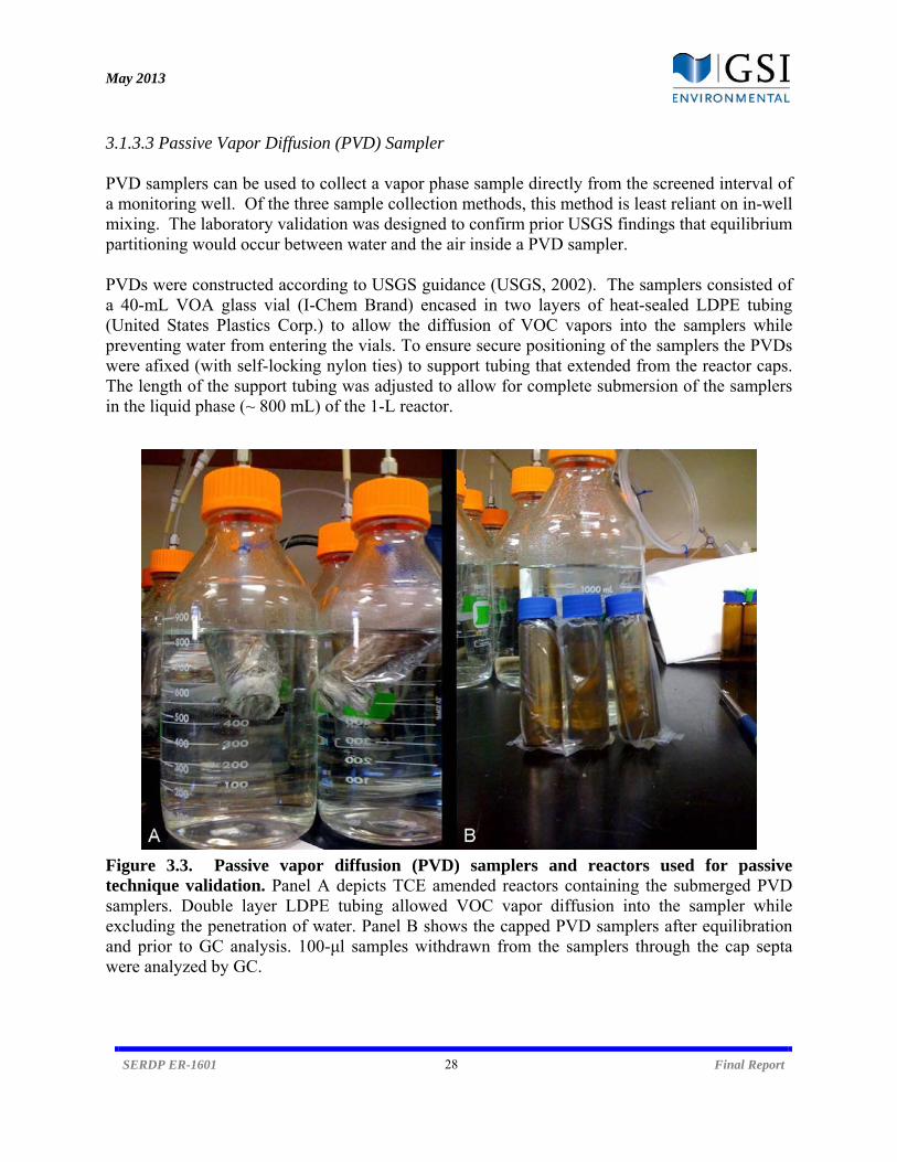
May 2013
SERDP ER-1601 28 Final Report
3.1.3.3 Passive Vapor Diffusion (PVD) Sampler PVD samplers can be used to collect a vapor phase sample directly from the screened interval of a monitoring well. Of the three sample collection methods, this method is least reliant on in-well mixing. The laboratory validation was designed to confirm prior USGS findings that equilibrium partitioning would occur between water and the air inside a PVD sampler. PVDs were constructed according to USGS guidance (USGS, 2002). The samplers consisted of a 40-mL VOA glass vial (I-Chem Brand) encased in two layers of heat-sealed LDPE tubing (United States Plastics Corp.) to allow the diffusion of VOC vapors into the samplers while preventing water from entering the vials. To ensure secure positioning of the samplers the PVDs were afixed (with self-locking nylon ties) to support tubing that extended from the reactor caps. The length of the support tubing was adjusted to allow for complete submersion of the samplers in the liquid phase (~ 800 mL) of the 1-L reactor.
Figure 3.3. Passive vapor diffusion (PVD) samplers and reactors used for passive technique validation. Panel A depicts TCE amended reactors containing the submerged PVD samplers. Double layer LDPE tubing allowed VOC vapor diffusion into the sampler while excluding the penetration of water. Panel B shows the capped PVD samplers after equilibration and prior to GC analysis. 100-μl samples withdrawn from the samplers through the cap septa were analyzed by GC.
May 2013
SERDP ER-1601 29 Final Report
Four experimental bottles were prepared to determine the time necessary to achieve equilibration of the VOCs between the reactor aqueous phase and the PVD sampler, and to validate this sampling method. A USGS study (2002) previously determined that equilibration time of the PVD is 1 to 3 weeks in similar settings. An aliquot of a methanol-based stock solution of TCE was delivered to each reactor to achieve an equilibrium water phase TCE concentration of 440 μg/L at 20°C. Analyses were conducted at approximately 3, 8, 16, and 23 days after the initial setup, with a bottle sacrificed for each analysis. At the time of sampling, the headspace of the 1-L reactor was evacuated into a Tedlar bag and analyzed with the portable GC instrument. The reactor was then opened and the PVD sampler was removed from the aqueous phase. The protective outer LDPE membrane layer was cut open and the vial (sealed in the inner LDPE membrane) was immediately capped by screwing the original cap (with Teflon/silicone septa) onto the vial. The vapor concentration of the PVD was analyzed in triplicate (100 μL samples) with the portable GC. The final aqueous phase VOC concentrations were also measured with laboratory gas chromatographs to provide additional validation parameters. 3.2 Temperature Study Vertical temperature gradients and effect on volatile organic compound (VOC) concentrations measured by low flow and passive diffusion bag samples were evaluated at two shallow monitoring wells at a site in Houston, Texas (the same site labeled as Site 3 during subsequent field programs described in the next section) . At each well, temperatures were measured hourly at four elevations for more than one year. Temperatures were measured using Model DS1921G iButton temperature data loggers in a Model DS9107 protective case from Maxim. This device operates without external power, can be placed in a monitoring well, and records temperature with a resolution of 0.5°C. The four measurement elevations covered the interval from the water surface to the bottom of the well screen in one well (MW-53) and from the water surface to the top of the well screen in the other well (MW-51; see Figure 1). In Well MW-51, silt or some other obstruction prevented access the lower portions of the screened interval. In order to characterize the vertical distribution of VOCs within the two wells, VOC concentrations were measured in November 2009 and May 2010 at same four elevations using passive diffusion samplers and at the lowest elevation using low flow sampling. At each well, VOC concentrations were also measured at one or more elevations on six other dates between 2006 and 2010. During the two primary monitoring events in November 2009 and May 2010, sample collection methods for analyzing groundwater VOC concentrations included passive diffusion bags placed at four different depth intervals (roughly corresponding to the middle of the screen and the other three depths where iButtons were placed) as well as a low-flow sample. All analyses were completed at a commercial laboratory (TestAmerica, Houston, Texas).

May 2013
SERDP ER-1601 30 Final Report
Figure 3.4. Simplified cross-section for monitoring wells included in temperature study. Bar indicates well screened interval, (x) indicates elevation of temperature probes, water elevation symbols indicate observed range of water elevation in wells, GL = ground elevation, TD = total depth.
The observed temperatures were compared to expected temperatures using the following equation for uniform soils (Hillel, 1982):
( ,t) = + − / 2( − /365− − /2 Where T(z,t) is the soil temperature at time t (days from the start of the year) and depth z (m), Ta is the average soil temperature (°C), A0 is the annual amplitude of the surface soil temperature (i.e., the difference between the maximum and minimum surface soil temperature, °C), d is the damping depth (m) of annual fluctuation and t0 is the time lag (days) from the start of the year to the occurrence of the minimum temperature in a year. The damping depth is given by d = (2Dh/w)0.5, where Dh is the thermal diffusivity and w, the frequency of the temperature variation, is 2π/365 d-1. Thermal diffusivity was assumed to be 0.07 m2/d, a value recommended by Nofziger and Wu, 2003 for soils with high clay content and high water content, representative of our site. Although the actual thermal diffusivity will vary with depth due to changes in soil saturation (i.e., above vs. below the water table), this simple model only supports use of a single value for thermal diffusivity. As recommended by Nofziger and Wu, 2003, the maximum and minimum surface soil temperatures were initially assumed to 2°C warmer than the maximum
May 2013
SERDP ER-1601 31 Final Report
(33.7°C) and minimum (4.3°C) daily average air temperature (Nofziger and Wu, 2003) at the site during this period. However, the final maximum and minimum soil temperature values of 37°C and 9°C, respectively, were adjusted from the recommended values to improve model fit. 3.3 Field Programs (Preliminary, Expanded, and Supplemental) 3.3.1 Site Selection The objective of the site selection process was to identify a large number wells that were suitable for the proposed field tests using a set of pre-established criteria. The primary criterion was to select sites located within 100 miles of the GSI office to ensure that excessive travel would not be required to collect data. After identifying a set of sites that met this primary criterion, the following criteria were used for further screening (Table 3.2):
Table 3.2. Primary Site Selection Criteria. Parameter Preferred Value(s)
Constituent Type(s) At least 1 volatile constituent
Concentration (aqueous-phase) At least 1 well with concentration below or near MCL
Site Access No restrictions
Well Diameter > 2 in.
Availability of Long-Term Monitoring Data Yes This screening process was repeated for each of the project phases, with one to five sites chosen depending on the phase. These sites—which are referred to by number to maintain confidentiality—meet the majority of the criteria, including all of those with the highest relevant importance. For the sites that were not selected, the primary reason was due to access limitations. In general, these eliminated sites required advance notice or special permission in order to enter the property, such that delays or refusals may have occurred if these were selected for individual field programs. Further, Site 1 was not included beyond the first phase of field testing because GSI’s work obligations at the site ended during the course of the project.
The number of wells selected for each of the field programs is listed in Table 3.3. This list includes several wells from each of the selected sites, as well as a number of different volatile constituents and well characteristics. A full list of all wells, with corresponding construction details and aquifer characteristics, are included in Appendix A. 3.3.2 Sampling Methods Table 3.4 summarizes the various sampling methods used during each phase of the project. Additional details on sampling procedures are provided in the following subsections as a reference.
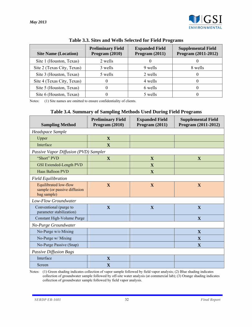
May 2013
SERDP ER-1601 32 Final Report
Table 3.3. Sites and Wells Selected for Field Programs
Site Name (Location) Preliminary Field Program (2010)
Expanded Field Program (2011)
Supplemental Field Program (2011-2012)
Site 1 (Houston, Texas) 2 wells 0 0
Site 2 (Texas City, Texas) 3 wells 9 wells 8 wells
Site 3 (Houston, Texas) 5 wells 2 wells 0
Site 4 (Texas City, Texas) 0 4 wells 0
Site 5 (Houston, Texas) 0 6 wells 0
Site 6 (Houston, Texas) 0 5 wells 0 Notes: (1) Site names are omitted to ensure confidentiality of clients.
Table 3.4. Summary of Sampling Methods Used During Field Programs
Sampling Method Preliminary Field Program (2010)
Expanded Field Program (2011)
Supplemental Field Program (2011-2012)
Headspace Sample Upper X Interface X
Passive Vapor Diffusion (PVD) Sampler “Short” PVD X X X GSI Extended-Length PVD X Haas Balloon PVD X
Field Equilibration Equilibrated low-flow sample (or passive diffusion bag sample)
X X X
Low-Flow Groundwater Conventional (purge to parameter stabilization)
X X X
Constant High-Volume Purge X No-Purge Groundwater
No-Purge w/o Mixing X No-Purge w/ Mixing X No-Purge Passive (Snap) X
Passive Diffusion Bags Interface X Screen X
Notes: (1) Green shading indicates collection of vapor sample followed by field vapor analysis; (2) Blue shading indicates collection of groundwater sample followed by off-site water analysis (at commercial lab); (3) Orange shading indicates collection of groundwater sample followed by field vapor analysis.
May 2013
SERDP ER-1601 33 Final Report
3.3.2.1 Preliminary Field Program The primary objective was of this phase of field testing was to assess whether the simple headspace methods provided reasonable results by collecting groundwater and vapor samples from various vertical locations within the well as a basis for comparison and to determine the extent of stratification. A total of seven different sampling methods were included as part of the field program. These methods are displayed in Figure 3.5 and described below. Note that to collect such a large number of samples within the same well, special well caps had to be designed and installed in advance of the first monitoring event. These were constructed by project personnel using modified compression caps and tested prior to use to ensure the seal integrity (Figure 3.6).
1. Upper Headspace: A vapor sample was collected from a port that terminated immediately below the sealed well cap. The port consisted of a short piece of rigid tubing that was installed through a small hole drilled in the cap and then held in place using silicon caulking. The port exited the top of the cap and was connected to a three-way valve via flexible tubing. The vapor sample was collected by connecting a disposal plastic syringe (60-mL) to the tubing and then opening the valve. Vapor samples were transferred to a Tedlar bag and allowed to equilibrate for several minutes. A 100-L vapor sample was then injected into the field GC for analysis. This represents the simplest method for collecting and analyzing vapor samples. Factors that contribute to accuracy include the presence of a suitable well seal and a uniformly-mixed air column above the water level.
2. Water-Vapor Interface: A second vapor sample was collected by drilling a second hole in the well cap and installing a vapor port that extended to a location immediately above the water-vapor interface. Like the upper headspace sampling method, this sample was collected using a short piece of tubing that connected the port with a three-way valve, and the vapor samples were transferred to a Tedlar bag prior to analysis with the field GC. The objective of collecting samples at the interface was to determine if poor mixing and/or limited diffusion within the air column was impacting accuracy, such that interface samples provide a more representative method of determining equilibrium groundwater concentrations.

May 2013
SERDP ER-1601 34 Final Report
Figure 3.5. Sampling Methods Tested During Preliminary Field Program .
Figure 3.6. Sampling Protocol During Preliminary Field Program
Well cap and sampling tubing with 60-mL syringes used for collecting separate vapor from the well upper headspace and water-vapor interface.
Vapor samples from the well upper headspace and water-vapor interface evacuated into Tedlar bags and analyzed by PID and a field GC. Separate vapor samples sent for lab analysis. .
Demonstrating the well assembly of the PVD (top) and PDB installed at screen (PDB installed at interface not shown). Low-flow groundwater samples collected as final step.
May 2013
SERDP ER-1601 35 Final Report
3. Passive Vapor Diffusion (PVD) Sampler at Screen: The final vapor sampling method involved placing a 40-mL VOA vial nylon-tied to a piece of support tubing at the center of the screened interval (see Figure 3.7). The vial was sealed in two layers of gas-permeable LDPE membrane. Following submersion below the water surface, this configuration prevents water from entering the vial but permits passive diffusion of vapor-phase contaminants across the membrane. Extended deployment within a well allowed for equilibration to occur, and the samplers were retrieved and then crimp-capped. A 100-L vapor sample from the vial was then collected and transferred to the field GC for analysis of organic constituents. Because the sampler body is rigid and the plastic outer layers are tight, there is minimal opportunity for the vapor within the sampler to expand once it is retrieved from a well. As such, in situ pressures can be maintained at the surface. However, additional pressure corrections were necessary because the syringes used in transferring vapor from the samplers to the analytical instruments were not pressure tight, such that the samples depressurized prior to analysis.
These PVD samplers were constructed in a manner identical to that described by USGS (2002). The notable difference is that the current project deployed them within a monitoring well at the screen to determine groundwater concentrations at equilibrium, as opposed to the USGS’s focus on the sediment-surface water interface. Note that in later phases of field testing, these were referred to as “short” PVDs to differentiate them from longer passive samplers (2.5-ft or greater).
4. Passive Diffusion Bag (PDB) at Water-Vapor Interface: Passive diffusion bags—consisting of 24-in long and 1.25-in diameter sealed LDPE bags filled with deionized water—were installed at the water-vapor interface using a string that connected the top of the bag with a loop on the underside of the well cap. Using static water level data collected prior to deployment, string lengths for individual wells were chosen that ensured complete water submersion of bag samplers. Similar to the PVD samplers, diffusion of organic contaminants across the gas-permeable membrane permits equilibration of the concentration in the monitoring well with the concentration of the water inside the sampler. Following retrieval of the PDB samplers from monitoring wells, water was transferred to 40-mL VOA vials using a screw-cap located at the top of the bags. Vials were then shipped to a commercial lab for analysis. PDB samples from the interface were collected in an attempt to demonstrate potential impacts of vertical stratification on correlations between headspace and groundwater samples.
5. Passive Diffusion Bag (PDB) at Screen: PDB bags were also installed at the screened interval using the same stringing technique with a weight attached to the bottom to minimize movement. Samples were collected in a manner identical to that described previously, and then shipped for off-site analysis at a commercial lab. Because these samples were collected from the middle of the screened interval, they were intended to provide a direct basis for comparison to low-flow groundwater samples and PVD samples.
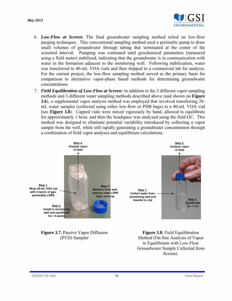
May 2013
SERDP ER-1601 36 Final Report
6. Low-Flow at Screen: The final groundwater sampling method relied on low-flow purging techniques. This conventional sampling method used a peristaltic pump to draw small volumes of groundwater through tubing that terminated at the center of the screened interval. Pumping was continued until geochemical parameters (measured using a field meter) stabilized, indicating that the groundwater is in communication with water in the formation adjacent to the monitoring well. Following stabilization, water was transferred to 40-mL VOA vials and then shipped to a commercial lab for analysis. For the current project, the low-flow sampling method served as the primary basis for comparison to alternative vapor-phase based methods for determining groundwater concentrations.
7. Field Equilibration of Low-Flow at Screen: In addition to the 3 different vapor sampling methods and 3 different water sampling methods described above (and shown on Figure 3.6), a supplemental vapor analysis method was employed that involved transferring 20-mL water samples (collected using either low-flow or PDB bags) to a 40-mL VOA vial (see Figure 3.8). Capped vials were mixed vigorously by hand, allowed to equilibrate for approximately 1 hour, and then the headspace was analyzed using the field GC. This method was designed to eliminate potential variability introduced by collecting a vapor sample from the well, while still rapidly generating a groundwater concentration through a combination of field vapor analyses and equilibrium calculations.
Figure 3.7. Passive Vapor Diffusion (PVD) Sampler
Figure 3.8. Field Equilibration Method (On-Site Analysis of Vapor
in Equilibrium with Low-Flow Groundwater Sample Collected from
Screen).
May 2013
SERDP ER-1601 37 Final Report
3.3.2.2 Expanded Field Program The expanded field program retained several of the methods that were shown to be promising during the previous field program, specifically the passive vapor diffusion (PVD) sampler and the field equilibration method. Low-flow groundwater samples were again included to serve as a baseline to vapor-based groundwater concentration estimates. Two additional passive vapor sampling methods were employed in an effort to develop better correlations with concentrations based on groundwater concentrations:
1. “Extended-Length” Passive Vapor Diffusion (PVD) Samplers: To overcome one potential shortcoming of the standard “short” PVD samplers (i.e., 40-mL vials), an extended-length PVD sampler was fabricated using a modified bailer wrapped in layered gas-permeable membrane that is heat-sealed to prevent water intrusion. By increasing the length of the sampler to approximately 60 inches, a larger surface area was available for diffusion (see Appendix C). This design also ensures that the sampler will coincide with a larger portion of the screen, in a manner similar to passive water diffusion bags. A similar equilibration period is needed. Following retrieval from the well, sufficient volume is available (> 500 mL) such that vapor samples can be transferred from the sampler to the field GC via syringe, or to a Tedlar bag for analyses via the PID or HAPSITE.
Because these samplers are not rigid, they are allowed to expand once they are removed from a well and hydrostatic pressure is relieved. As such, additional pressure corrections were necessary when calculating the equivalent groundwater concentration to account for the lower mass-per-volume ratios at the surface relative to in situ conditions.
2. Haas/AFCEE “Balloon” Samplers: An alternative passive sampling device developed by P.E. Haas & Associates LLC and AFCEE was also tested in cooperation with Patrick Haas. The design used for this project consisted of a flexible membrane polyethylene sealed bag measuring approximately 30 inches in length (see Appendix C). The sampler is pressurized with nitrogen during installation and then allowed to equilibrate within the well (Note that nitrogen was selected as opposed to air to avoid introducing oxygen to the well). When ready to be sampled, vapor was collected by depressurizing the bag using tubing that connects the bag to the surface. This procedure can eliminate the sampler retrieval step, although samplers were retrieved during the current study to confirm that they were holding pressure and that there were no leakage issues.
Similar to the “extended-length” PVDs, these balloon samplers are allowed to expand once they are removed from a well and hydrostatic pressure is no longer an influence. This necessitates a pressure correction step when calculating the equivalent groundwater concentration. If the samplers are left in the well during the sample collection process (i.e., not retrieved), then pressure corrections are not necessary if a pressure-lock syringe is used to transfer the vapor sample to the analytical equipment.
May 2013
SERDP ER-1601 38 Final Report
3.3.2.3 Supplemental Field Program The supplemental field program again used the passive vapor diffusion (PVD) sampler and the field equilibration method for estimating groundwater concentrations. Low-flow groundwater samples were also included to serve as a baseline to vapor-based groundwater concentration estimates. Because a primary objective was to demonstrate if the variability associated with vapor-based concentration estimates is similar to that associated with measured groundwater concentrations, the program also included several additional low-flow and no-purge groundwater samples during selected events. These groundwater samples were part of the SERDP ER-1705 monitoring program that was conducted jointly with the SERDP ER-1601 program, and provided a basis for comparing monitoring data variability and methods to reduce that variability:
1. Low-Flow Purge with Constant Purge Volume: Groundwater samples were collected in accordance with standard low-flow purge procedures. However, rather than sampling to purge parameter stability, a constant purge volume of 24L was used. This purge volume is equal to four screen volumes and should be sufficient to achieve steady-state flow conditions within the monitoring well screened interval.
2. No Purge Passive Sampling: Groundwater sample was collected using Snap passive sampling system during selected events. The Snap sampling system provides very consistent sample collection between sample events (e.g., consistent sample depth). In addition, the groundwater sample is not exposed to the atmosphere during sample collection, eliminating variability associated with loss of volatiles to the atmosphere.
3. No Purge Low-Flow Sampling with In-well Mixing: Groundwater samples were collected using low flow sampling procedures. However, the screened interval was isolated from the well casing using a baffle installed at least three weeks prior to sample collection. Prior to sample collection, the water within the screened interval was physically mixed. Following mixing, the sample was then collected without purging.
4. No Purge Low-Flow Sampling without In-Well Mixing: Groundwater samples were collected in accordance with standard low-flow purge procedures but without purging to parameter stability (i.e., immediate collection of the sample). The results obtained using this sample collection method provided an improved understanding of the effect of in-well mixing on the sample results.
3.3.3 Analytical Methods Two devices described previously—the field-portable GC and the PID—were used extensively during field testing. The field-portable GC was used during all phases, while the PID was used during the preliminary field program and the expanded field program. A third device was added to the expanded field program, the HAPSITE ER Chemical Identification System (manufactured by INFICON). This device has been used extensively in environmental monitoring applications, typically for emergency response and vapor intrusion. It

May 2013
SERDP ER-1601 39 Final Report
is well-suited for on-site applications, and uses a combination of gas chromatography and mass spectrometry to identify and quantify a variety of constituents of concern. It also has a survey mode for real-time quantification of single constituents. The HAPSITE has been tested as part of the USEPA’s Environmental Technology Verification Program for simple wellhead applications (i.e., groundwater-based analyses). The manufacturer sells a headspace sampling system for field equilibration of water samples (aided by sample heating), though this system was not tested as part of this project. Sampling requirements for the various devices varied. The volume for the field GC was typically 100 L; larger or smaller volumes can be used (assuming that they are compatible with the internal volume of the sampling loop). The PID and HAPSITE require significantly higher volumes, on the order of 250 mL per sample. The PID provides a continuous signal, and the higher volume is designed to provide sufficient time for the user to get a consistent reading. The HAPSITE requires a high volume to flush through the entire sampling loop. In general, 250 mL of sample were transferred to large-volume Tedlar bags (1 L) prior to measuring with either the PID or the HAPSITE. In cases where limited sample volume was available, samples were diluted with equal volumes of nitrogen gas. All analytical equipment were calibrated daily using standard gases composed of expected site constituents (e.g., VC, TCE, 1,1-DCE). A minimum of two-point calibrations were performed. Note that syringes used in transferring vapor samples to the analytical equipment were gas tight (i.e., prevented external air from entering syringe during sample collection) but not pressure tight. 3.3.4 Sampling and Analysis Plans 3.3.4.1 Preliminary Field Program The intensive monitoring program was conducted in 10 monitoring wells in the Houston area over the course of approximately 6 weeks (Table 3.5). At each site, well materials (caps, passive sampling devices) were installed in a single mobilization in December 2009 at the onset of the study. A monitoring event was then completed in January 2010, approximately 3 weeks after this installation event, at an interval that is appropriate for passive diffusion samplers based on technology guidance documents. At the conclusion of this monitoring event, well materials were replaced, and then a second monitoring event was completed in February 2010 after another 3-week period had elapsed. The sampling and analysis plan included the methods outlined in Section 3.3.2.1 and summarized in Table 3.6: 3 different vapor sampling methods and 3 different water sampling methods, as well as a supplemental vapor analysis method that involves transferring water samples (collected using either low-flow or PDB bags) to a small vial and then analyzing the vapor in equilibrium with that water. Following receipt and review of data from the first
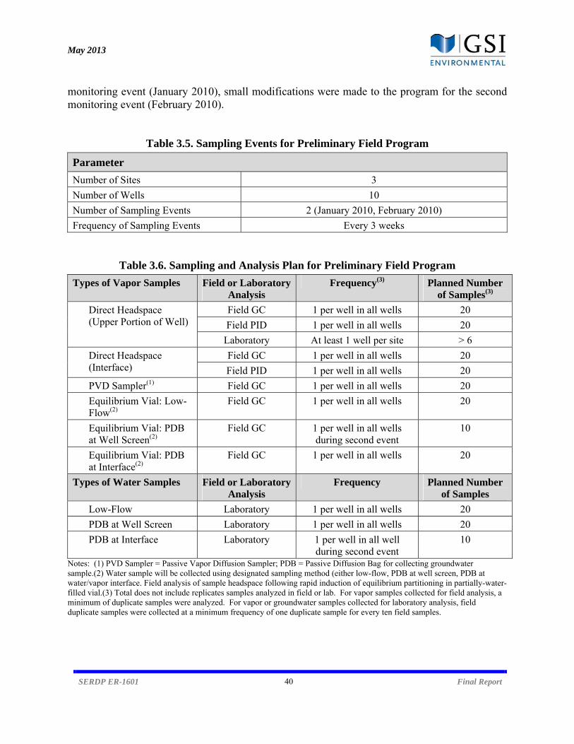
May 2013
SERDP ER-1601 40 Final Report
monitoring event (January 2010), small modifications were made to the program for the second monitoring event (February 2010).
Table 3.5. Sampling Events for Preliminary Field Program
Parameter Number of Sites 3
Number of Wells 10
Number of Sampling Events 2 (January 2010, February 2010)
Frequency of Sampling Events Every 3 weeks
Table 3.6. Sampling and Analysis Plan for Preliminary Field Program Types of Vapor Samples Field or Laboratory
Analysis Frequency(3) Planned Number
of Samples(3) Direct Headspace (Upper Portion of Well)
Field GC 1 per well in all wells 20
Field PID 1 per well in all wells 20
Laboratory At least 1 well per site > 6
Direct Headspace (Interface)
Field GC 1 per well in all wells 20
Field PID 1 per well in all wells 20
PVD Sampler(1) Field GC 1 per well in all wells 20
Equilibrium Vial: Low-Flow(2)
Field GC 1 per well in all wells 20
Equilibrium Vial: PDB at Well Screen(2)
Field GC 1 per well in all wells during second event
10
Equilibrium Vial: PDB at Interface(2)
Field GC 1 per well in all wells 20
Types of Water Samples Field or Laboratory Analysis
Frequency Planned Number of Samples
Low-Flow Laboratory 1 per well in all wells 20
PDB at Well Screen Laboratory 1 per well in all wells 20
PDB at Interface Laboratory 1 per well in all well during second event
10
Notes: (1) PVD Sampler = Passive Vapor Diffusion Sampler; PDB = Passive Diffusion Bag for collecting groundwater sample.(2) Water sample will be collected using designated sampling method (either low-flow, PDB at well screen, PDB at water/vapor interface. Field analysis of sample headspace following rapid induction of equilibrium partitioning in partially-water-filled vial.(3) Total does not include replicates samples analyzed in field or lab. For vapor samples collected for field analysis, a minimum of duplicate samples were analyzed. For vapor or groundwater samples collected for laboratory analysis, field duplicate samples were collected at a minimum frequency of one duplicate sample for every ten field samples.

May 2013
SERDP ER-1601 41 Final Report
Field analysis of vapor samples was completed using the field instruments (both the field-portable GC and the PID), with a low-flow purge groundwater sample collected as the primary basis for comparison. The VOC concentration in low-flow groundwater samples was completed at a commercial analytical lab (TestAmerica, Houston, Texas). In addition, lab analyses of samples from passive water diffusion bags installed at both the well screen and at the water-vapor interface were completed at a subset of wells to compare to samples from the PVD samplers as well as low-flow samples. At select wells, an additional vapor analysis was conducted by placing the water sample in a sealed container containing a headspace and agitating the sample for a sufficient period of time to achieve equilibrium partitioning. A field measurement of the headspace was then used to determine the VOC concentration in the water sample (Figure 3.8). A final sample type consisted of lab analysis of vapor samples collected with a Tedlar bag from the well headspace. Independent commercial laboratories (TestAmerica or Columbia Analytical) were used for all off-site analyses. In order to minimize the effect of sample collection on the sample results, the samples were collected from each well in sequential order with the samples most likely to be affected by short-term mixing/disturbance collected first. The sample collection order was as follows:
1) Vapor analysis of well headspace samples from top of well 2) Vapor analysis of well headspace samples from close to water table 3) Removal of passive diffusion samplers from monitoring well; transfer of water to 40-mL
VOA vials for lab analysis 4) Removal of passive water diffusion samplers; transfer of water to 40-mL VOA vials for
lab analysis 5) Collection of low-flow water samples for lab analysis 6) Vapor analysis of water samples in equilibration vials
3.3.4.2 Expanded Field Program The expanded field program was conducted in a larger set of monitoring wells (26) selected based on the same screening criteria described previously. It again included two monitoring events at each well (Table 3.7).
Table 3.7. Sampling Events for Expanded Field Program Parameter Number of Sites 5
Total Number of Wells 26
Number of Sampling Events 2 (April 2011, May 2011)
Frequency of Sampling Events Every 3 weeks
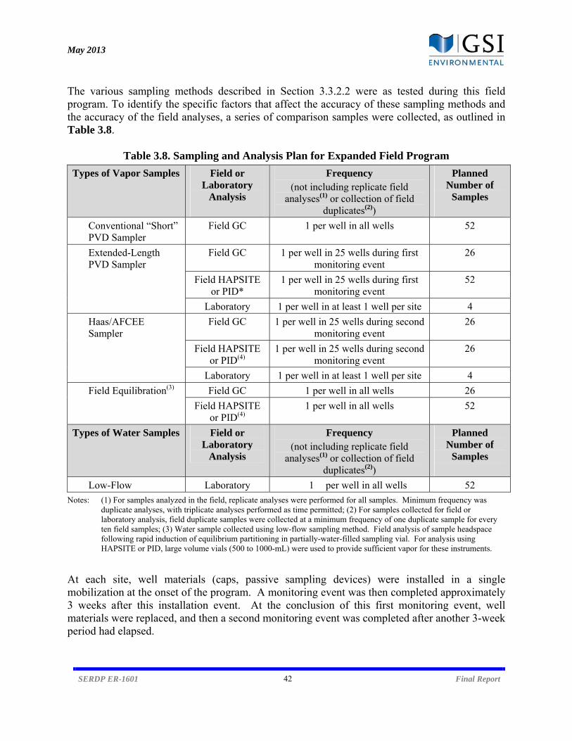
May 2013
SERDP ER-1601 42 Final Report
The various sampling methods described in Section 3.3.2.2 were as tested during this field program. To identify the specific factors that affect the accuracy of these sampling methods and the accuracy of the field analyses, a series of comparison samples were collected, as outlined in Table 3.8.
Table 3.8. Sampling and Analysis Plan for Expanded Field Program Types of Vapor Samples Field or
Laboratory Analysis
Frequency (not including replicate field
analyses(1) or collection of field duplicates(2))
Planned Number of
Samples
Conventional “Short” PVD Sampler
Field GC 1 per well in all wells 52
Extended-Length PVD Sampler
Field GC 1 per well in 25 wells during first monitoring event
26
Field HAPSITE or PID*
1 per well in 25 wells during first monitoring event
52
Laboratory 1 per well in at least 1 well per site 4
Haas/AFCEE Sampler
Field GC 1 per well in 25 wells during second monitoring event
26
Field HAPSITE or PID(4)
1 per well in 25 wells during second monitoring event
26
Laboratory 1 per well in at least 1 well per site 4
Field Equilibration(3) Field GC 1 per well in all wells 26
Field HAPSITE or PID(4)
1 per well in all wells 52
Types of Water Samples Field or Laboratory
Analysis
Frequency (not including replicate field
analyses(1) or collection of field duplicates(2))
Planned Number of
Samples
Low-Flow Laboratory 1 per well in all wells 52 Notes: (1) For samples analyzed in the field, replicate analyses were performed for all samples. Minimum frequency was
duplicate analyses, with triplicate analyses performed as time permitted; (2) For samples collected for field or laboratory analysis, field duplicate samples were collected at a minimum frequency of one duplicate sample for every ten field samples; (3) Water sample collected using low-flow sampling method. Field analysis of sample headspace following rapid induction of equilibrium partitioning in partially-water-filled sampling vial. For analysis using HAPSITE or PID, large volume vials (500 to 1000-mL) were used to provide sufficient vapor for these instruments.
At each site, well materials (caps, passive sampling devices) were installed in a single mobilization at the onset of the program. A monitoring event was then completed approximately 3 weeks after this installation event. At the conclusion of this first monitoring event, well materials were replaced, and then a second monitoring event was completed after another 3-week period had elapsed.
May 2013
SERDP ER-1601 43 Final Report
The size of several of the samplers precluded their simultaneous deployment, meaning that they would have to be installed at different depths and would collect groundwater from different sections of the screened interval. Due to the potential for vertical stratification, this would introduce unnecessary variability into the datasets. Instead, the devices were tested in phases. The extended-length PVD was used during the first monitoring event, while the Haas/AFCEE balloon sampler was used during the second follow-up monitoring event. The short PVD sampler was installed in all wells during both events, immediately above whichever of the other PVD samplers was also installed during that monitoring phase. Field analysis of all vapor samples will be conducted using the field GC, and the HAPSITE and/or a PID meter. Note that since the minimum volume requirements for these latter two instruments (typically 250 mL) was large relative to the volume of the in-well sampling devices, the use of both instruments at the same well was frequently precluded. Low-flow groundwater samples were collected at all wells and sent to an off-site commercial lab, with the data serving as a basis for comparison with concentrations determined using vapor-phase field analyses. As documented in the previous phase of field testing, there are occasions when low-flow groundwater and passive groundwater samples return different results. However, as noted above, the dimensions of the various sampling devices preclude the co-deployment of passive water bags and the longer of the passive vapor samplers. As noted in Table 3.8, field equilibration of low-flow groundwater samples was also performed at select wells, followed by field analysis of the equilibrated vapor. A final sample type consisted of lab analysis of vapor collected with the extended-length PVD sampler or the Hass/AFCEE balloon sampler and then transferred to Tedlar bags. Data from these analyses was used to assess the accuracy and precision of the field equipment. Independent commercial laboratories (TestAmerica, Houston, Texas; Columbia Analytical Services, Simi Valley, California) were used for all off-site analyses of groundwater and vapor samples. In order to minimize the effect of sample collection on the sample results, the samples were collected from each well in sequential order with the samples most likely to be affected by short-term mixing/disturbance collected first. The sample collection order was as follows: 3.3.4.2 Supplemental Field Program The program involved the implementation of these sampling methods multiple times in a series of 8 wells over the course of 43 weeks. Sampling events were completed approximately every 3 weeks during this period. Various vapor and groundwater sampling methods were used during individual events to determine the impact of particular modifications on sampling variability over time. Using the SERDP ER-1705 sampling plan as a basis, the following program was developed:

May 2013
SERDP ER-1601 44 Final Report
Table 3.9. Summary of Supplemental Field Program: Joint Program with SERDP ER-1705 SERDP ER-1705 Sample Method (groundwater methods)
Supplemental SERDP ER-1601 Sample Method(s) (vapor-based methods)
Preparatory Activities for Next Sampling Event
Completion Schedule
Low-Flow Sampling with Purge to Parameter Stability
1) Field equilibration with low flow sample collected prior to purge
2) Field equilibration with low flow sample collected after purge
3) Short PVDs at 3 different depths 4) Low-flow sample prior to purge
Install new set of PVDs. Leave dedicated low-flow collection tubing in well.
Weeks 11, 16, 31
Low-Flow Sampling with Constant Volume Purge (24 L)
1) Field equilibration with low flow sample collected prior to purge
2) Field equilibration with low flow sample collected after purge
3) Short PVDs at 3 different depths 4) Low-flow sample prior to purge
Install new set of PVDs. Leave dedicated low-flow collection tubing in well.
Weeks 4, 19, 34
No Purge Low Flow Sampling without In-Well Mixing
1) Field equilibration with low-flow sample prior to purging or mixing
2) Field equilibration with low-flow sample collected after purge
3) Short PVDs at 3 different depths 4) Low-flow sample following purge
Install new set of PVDs. Remove low-flow collection tubing. Install Snap sampler system.
Weeks 7, 22, 37
No purge passive sampling (Snap sampler)
1) Short PVDs at 3 different depths Remove Snap sampler system. Install mixing/sampling system.
Weeks 10, 25, 40
No Purge Low-Flow Sampling with In-Well Mixing
1) Field equilibration with low-flow sample after mixing
Remove mixing/sampling system. Install dedicated low-flow sample collection tubing. Install new set of PVDs.
Weeks 13, 28, 43
Notes: (1) Short PVD was not installed for Week 1 sampling
As indicated in Table 3.9, the field equilibration method and the PVD samplers are not compatible with all of the sampling methods/approaches being utilized for the SERDP ER-1705 program. For example, the short PVDs proved difficult to include in the system envisioned for in-well mixing. Similarly, as a time-savings measure, field equilibration of purged samples were not included if purging was not otherwise specified for the SERDP ER-1705 program. Regardless, each of the SERDP ER-1601 sampling methods was employed during at least 3 distinct events, ensuring that adequate data was generated for evaluation.
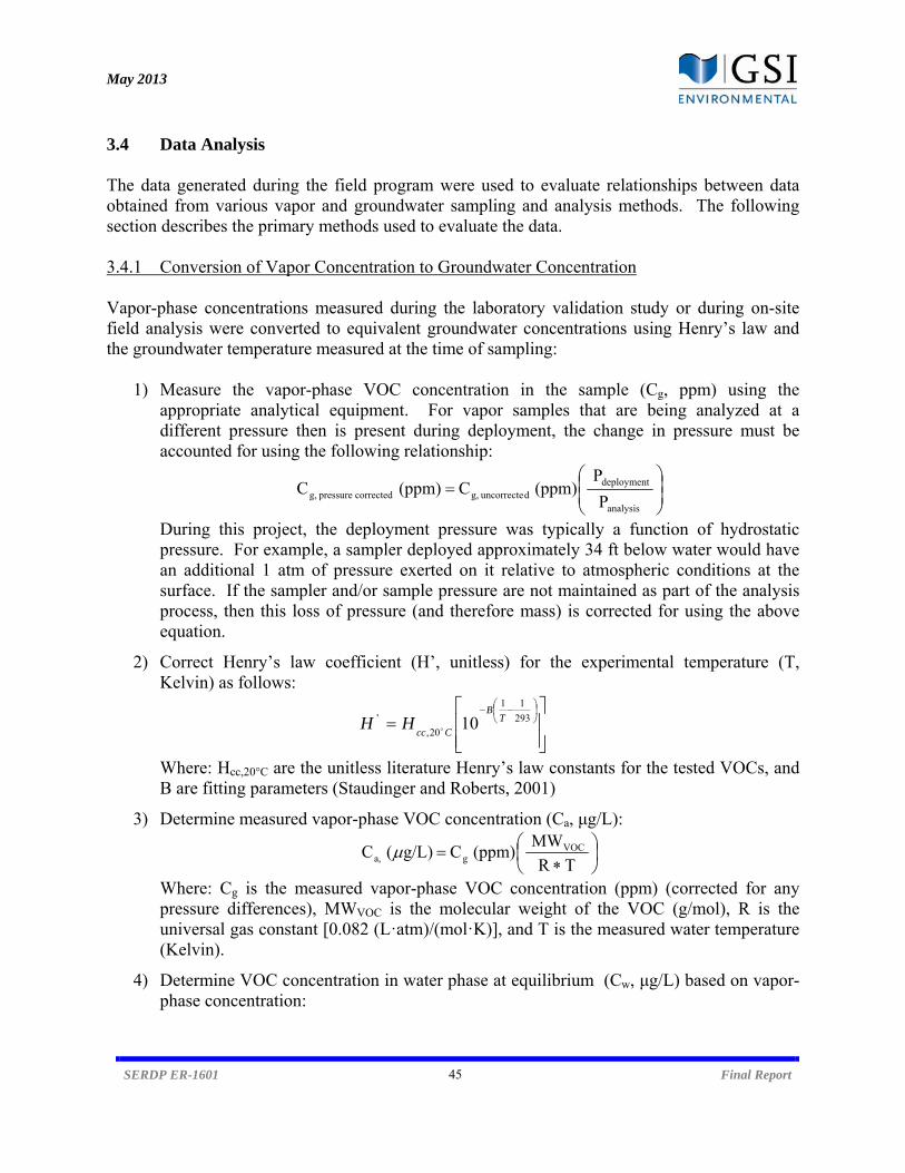
May 2013
SERDP ER-1601 45 Final Report
3.4 Data Analysis The data generated during the field program were used to evaluate relationships between data obtained from various vapor and groundwater sampling and analysis methods. The following section describes the primary methods used to evaluate the data. 3.4.1 Conversion of Vapor Concentration to Groundwater Concentration Vapor-phase concentrations measured during the laboratory validation study or during on-site field analysis were converted to equivalent groundwater concentrations using Henry’s law and the groundwater temperature measured at the time of sampling:
1) Measure the vapor-phase VOC concentration in the sample (Cg, ppm) using the appropriate analytical equipment. For vapor samples that are being analyzed at a different pressure then is present during deployment, the change in pressure must be accounted for using the following relationship:
analysis
deploymentduncorrecte g,corrected pressure g, P
P(ppm) C (ppm) C
During this project, the deployment pressure was typically a function of hydrostatic pressure. For example, a sampler deployed approximately 34 ft below water would have an additional 1 atm of pressure exerted on it relative to atmospheric conditions at the surface. If the sampler and/or sample pressure are not maintained as part of the analysis process, then this loss of pressure (and therefore mass) is corrected for using the above equation.
2) Correct Henry’s law coefficient (H’, unitless) for the experimental temperature (T, Kelvin) as follows:
293
11
20,
' 10 TB
CccHH
Where: Hcc,20°C are the unitless literature Henry’s law constants for the tested VOCs, and B are fitting parameters (Staudinger and Roberts, 2001)
3) Determine measured vapor-phase VOC concentration (Ca, μg/L):
TR
MW(ppm) C g/L)( C VOC
ga,
Where: Cg is the measured vapor-phase VOC concentration (ppm) (corrected for any pressure differences), MWVOC is the molecular weight of the VOC (g/mol), R is the universal gas constant [0.082 (L·atm)/(mol·K)], and T is the measured water temperature (Kelvin).
4) Determine VOC concentration in water phase at equilibrium (Cw, μg/L) based on vapor-phase concentration:
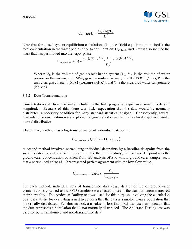
May 2013
SERDP ER-1601 46 Final Report
'a
W
g/L)( C g/L)( C
H
Note that for closed-system equilibrium calculations (i.e., the “field equilibration method”), the total concentration in the water phase (prior to equilibration; CW,Total, μg/L) must also include the mass that has partitioned into the vapor phase:
'
WWaTotalW,
V*g/L)( CV*g/L)( C g/L)( C
W
g
V
Where: Vg is the volume of gas present in the system (L), VW is the volume of water present in the system, and MWVOC is the molecular weight of the VOC (g/mol), R is the universal gas constant [0.082 (L·atm)/(mol·K)], and T is the measured water temperature (Kelvin).
3.4.2 Data Transformations Concentration data from the wells included in the field programs ranged over several orders of magnitude. Because of this, there was little expectation that the data would be normally distributed, a necessary condition for many standard statistical analyses. Consequently, several methods for normalization were explored to generate a dataset that more closely approximated a normal distribution. The primary method was a log-transformation of individual datapoints:
wed transformW, C LOG g/L)( C
A second method involved normalizing individual datapoints by a baseline datapoint from the same monitoring well and sampling event. For the current study, the baseline datapoint was the groundwater concentration obtained from lab analysis of a low-flow groundwater sample, such that a normalized value of 1.0 represented perfect agreement with the low-flow value.
flow-low w,
wed transformW, C
C g/L)( C
For each method, individual sets of transformed data (e.g., dataset of log of groundwater concentrations obtained using PVD samplers) were tested to see if the transformation improved their normality. The Anderson-Darling test was used for this purpose, involving the calculation of a test statistic for evaluating a null hypothesis that the data is sampled from a population that is normally distributed. For this method, a p-value of less than 0.05 was used an indicator that the data represents a population that is not normally distributed. The Anderson-Darling test was used for both transformed and non-transformed data.

May 2013
SERDP ER-1601 47 Final Report
3.4.3 Linear Regression Analysis Regression analysis was the primary means for examining relationships between the various concentration datasets generated in each of the phases of field testing. A linear trend between two (log-transformed) datasets generated from the same population (i.e., the same set of wells) was assumed, and this standard parametric test was employed. Simple linear regression analysis between two datasets that are expected to be similar provides two primary metrics:
R2 as an indicator of variability: The R2 value (or the squared correlation coefficient) demonstrates the “goodness-of-fit”, with higher values (near one) indicating a better fit. Because low values of R2 represent a large degree of scatter in the residuals, they are a strong indicator of variability.
Slope as an indicator of bias: The slope of the regression line can be used to evaluate a predictive relationship between the independent variable and the dependent variable. Since data used in the linear regression are collected from the same set of wells but using different methods, a slope near one would indicate that the datasets are similar. A slope of less than one would indicate under-prediction or low bias relative to the baseline case (e.g., groundwater concentration from a low-flow sample), and a slope greater than one suggests over-prediction or high bias.
Linear regressions were performed on log-transformed data using the Excel data analysis tool, with the origin of the regression line set as zero to correspond to the absence of the measured constituent in the analyzed media. When two datasets were compared, the regression generally included only those data points for which both methods resulted in a measurement above reporting limits. 3.4.4 Two-Sample Tests Simple two-sample tests were used as a statistical tool to evaluate potential differences between concentration datasets collected with the various sampling and analysis methods. These tests were employed during each of the phases of field testing since data were obtained from the same population (i.e., the same set of wells) and thus facilitated a paired comparison. For all cases, the low-flow groundwater sample was used as the baseline for comparison. In the current study, both non-parametric and parametric two-sample tests were conducted:
1. Wilcoxon Rank-Sum Test or Wilcoxon Signed-Rank Test (non-parametric): These tests take paired data, calculates the differences between each individual data pair, and then ranks the differences. The ranked data is sorted by sign, summed, and then used to
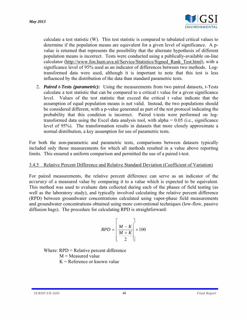
May 2013
SERDP ER-1601 48 Final Report
calculate a test statistic (W). This test statistic is compared to tabulated critical values to determine if the population means are equivalent for a given level of significance. A p-value is returned that represents the possibility that the alternate hypothesis of different population means is incorrect. Tests were conducted using a publically-available on-line calculator (http://www.fon.hum.uva.nl/Service/Statistics/Signed_Rank_Test.html), with a significance level of 95% used as an indicator of differences between two methods. Log-transformed data were used, although it is important to note that this test is less influenced by the distribution of the data than standard parametric tests.
2. Paired t-Tests (parametric): Using the measurements from two paired datasets, t-Tests calculate a test statistic that can be compared to a critical t value for a given significance level. Values of the test statistic that exceed the critical t value indicate that the assumption of equal population means is not valid. Instead, the two populations should be considered different, with a p-value generated as part of the test protocol indicating the probability that this condition is incorrect. Paired t-tests were performed on log-transformed data using the Excel data analysis tool, with alpha = 0.05 (i.e., significance level of 95%). The transformation results in datasets that more closely approximate a normal distribution, a key assumption for use of parametric tests.
For both the non-parametric and parametric tests, comparisons between datasets typically included only those measurements for which all methods resulted in a value above reporting limits. This ensured a uniform comparison and permitted the use of a paired t-test. 3.4.5 Relative Percent Difference and Relative Standard Deviation (Coefficient of Variation) For paired measurements, the relative percent difference can serve as an indicator of the accuracy of a measured value by comparing it to a value which is expected to be equivalent. This method was used to evaluate data collected during each of the phases of field testing (as well as the laboratory study), and typically involved calculating the relative percent difference (RPD) between groundwater concentrations calculated using vapor-phase field measurements and groundwater concentrations obtained using more conventional techniques (low-flow, passive diffusion bags). The procedure for calculating RPD is straightforward:
100
2
KMKM
RPD
Where: RPD = Relative percent difference
M = Measured value K = Reference or known value
May 2013
SERDP ER-1601 49 Final Report
The RPD can be used to compare individual data points as well as entire datasets. For the latter case, the median RPD for the dataset was used. The median RPD can be expressed as either non-directional (e.g., ignoring the sign) as an indicator of variability, or as directional (including the sign) as an indicator of bias. Similarly, a quantitative indicator of precision is the relative standard deviation (RSD) between two datapoints obtained using the same sampling technique or analytical method. The RSD can also be labeled the Coefficient of Variation (CV). The RSD (or CV) can be calculated for any dataset when replicates are collected using the following procedure:
100x
SRSD
Where: S is the variance of the replicate data set, and
x is the arithmetic mean of the replicate measurements.
3.4.6 Analysis of Variance (ANOVA) During the supplemental field program, data were collected from the same set of wells repeatedly but using different sampling/analysis methods. The primary method used to evaluate these datasets was ANOVA:
Analysis of Variance (ANOVA) using Coefficient of Variation: The variability in VOC concentrations between samples collected from the same well using the same method will be characterized using the coefficient of variation:
CV = S / x
Where CV = coefficient of variation for results from a single well
S = standard deviation for results from a single well
x = arithmetic mean for results from a single well
Based on the number of sample collection/analysis methods outlined in Table 4.8, this yielded 11 CV values per well. ANOVA was employed to determine if there was a difference in the average CVs between the different sampling methods. The objective was to determine if there is a statistically significant difference between the average CV for the baseline method (low-flow groundwater following purge to parameter stability) relative to average CVs associated with each of the alternative methods.
Analysis of Variance (ANOVA) using Mean: The potential bias in VOC concentrations between samples collected from the same well using the same method was characterized by calculating the mean concentration obtained using each individual method. This
May 2013
SERDP ER-1601 50 Final Report
yielded 11 mean values per well, or one for each of the sample collection/analysis methods outlined in Table 3.9. ANOVA was used to determine if the different sampling methods yield statistically-significant differences between the mean values obtained for the baseline method (low-flow groundwater following purge to parameter stability) relative to the mean values obtained using each of the alternative methods.
May 2013
SERDP ER-1601 51 Final Report
4. RESULTS AND DISCUSSION
Results obtained during this project are described in separate sections for each of the primary project tasks. These tasks are listed below along with key findings:
1. Laboratory Validation of Vapor-Phase Monitoring (Section 4.1): Both the field-portable GC and PID instruments achieved the target criteria for accuracy, precision, and sensitivity, such that these instruments were retained for further field testing. In terms of methods for collecting vapor-phase samples, direct headspace sampling and passive vapor diffusion (PVD) samplers also met performance objectives and were retained for field testing. Results of the lab study were published in Adamson et al. (2009).
2. Temperature Study (Section 4.2): The influence of seasonal temperature gradients on mixing within monitoring wells was demonstrated using a combination of model and field data. These effects contribute to vertical stratification of VOC concentrations during periods that were thermally stable (late summer), limiting the potential application of headspace methods in estimating groundwater concentration (which rely on flow-weighted averaging) while increasing the viability of depth-discrete sampling. A better understanding of prevailing thermal mixing conditions should be incorporated into the development of monitoring programs as well as interpretation of monitoring data. Results of the temperature study were published in McHugh et al. (2012).
3. Preliminary Field Study (Section 4.3): Strong correlations with groundwater concentrations were obtained using on-site analysis of samples collected from the screened interval of monitoring wells, either using passive vapor diffusion samplers or equilibrated vapor from groundwater samples. Correlations were relatively poor using the simple headspace collection method due to the presence of vertical stratification within the well, such that this method is not recommended except as a bulk indicator of groundwater concentrations. Results of the preliminary field study were published in Adamson et al. (2012).
4. Expanded Field Study (Section 4.4): Three different passive vapor diffusion sampler designs were tested at a larger number of wells, and the simplest design—a short sampler for collecting depth-discrete data—performed nearly identically to longer samplers. The similarly strong performance for sampler types that cover much different portions of the screened interval suggested that well-mixed conditions were prevalent during this sampling period. The field GC provided more accurate and less variable on-site results than other analytical equipment included in the study (PID and HAPSITE). Results will be combined with data from subsequent tasks for a guidance-focused manuscript to be submitted to a peer-reviewed journal in Spring 2013.
5. Supplemental Field Testing (Section 4.5): A longer-term field program was implemented to assess the amount of variability associated with the most promising vapor-phase based methods. The variability of concentration data obtained using passive vapor diffusion samplers and the field equilibration method were evaluated during several events completed over the course of nearly a year. No statistically significant

May 2013
SERDP ER-1601 52 Final Report
differences in variability were obtained when comparing the vapor-phase based data with data obtained using low-flow groundwater sampling (including no-purge samples, samples collected after in-well mixing, samples collected after purging fixed volumes, and samples collected after purging to parameter stability) or Snap samplers (i.e., passive groundwater samplers). In general, methods designed to reduce variability had little or no significant benefit. Results of the study will be combined with data from other tasks for a guidance-focused manuscript to be submitted to a peer-reviewed journal in Spring 2013.
6. Assessment of Cost-Effectiveness (Section 4.6): Direct comparisons between monitoring alternatives were evaluated based on “cost per sample” and other applicable metrics using extensive cost modeling. Various scenarios were developed and tested, showing that groundwater monitoring could be completed at a cost savings of at least 36% when on-site vapor-based monitoring was completed using a rented GC. This represents a savings of several hundred dollars per sample for typical monitoring programs (depending on whether monitoring was completed at an in-town or out-of-town site). Cost information will be included in the guidance-focused manuscript to be submitted to a peer-reviewed journal in Spring 2013.
The collective results were used to develop the guidance document for vapor-based groundwater monitoring methods that is Appendix C of this report. 4.1 Laboratory Validation Study The laboratory study was designed to validate the use of the instruments and vapor sampling methods based on a combination of accuracy, precision, and sensitivity. The following objectives were used to evaluate performance:
Accuracy: Target of RPD of +/-30% between paired data Precision: Target of RSD of +/-30% between paired data Sensitivity: Method detection limit (MDL) < Maximum Contaminant Level (MCL) for
all VOCs tested; ii) accuracy and precision objectives achieved at lowest concentration tested
4.1.1 Portable Field Instrument Validation Results 4.1.1.1 PID Validation The performance of the hand-held ppbRAE 3000 PID was evaluated through the measurement of pure gases and gas mixtures of known concentrations. As shown in Table 4.1, all measurements achieved the target accuracy and precision objectives of a RPD of +/-30% and a RSD of 30%. In addition, the calculated MDLs corresponded to dissolved VOC concentrations of < 5 g/L. The PID exhibited a consistent low bias of 10 to 20%, however, this low bias did not prevent attainment of the accuracy and precision objective.

May 2013
SERDP ER-1601 53 Final Report
Table 4.1. Accuracy, Precision, and Sensitivity of ppbRAE 3000 PID
VOC
Standard Concentration
(ppmv)
Number of Replicate
Measurements Accuracy Range
(RPD) Precision
(RSD) Sensitivity:
MDL (ppmv)
Benzene 1.04 7 -17.0% to -9.7% 2.7% 0.077
5 7 -20.2% to -15.6% 1.5% N/A(1) Mixture of 1,1-DCE, Benzene,
TCE
0.33 7 -22.5% to -5.3% 5.3% 0.079 3.06 7 -21.6% to -15.9% 2.3% N/A(1) 31.2 7 -17.3% to -14.5% 1.1% N/A(1)
Notes: (1) Method detection limit calculation applies only to the lowest concentration tested. Finding: The ppbRAE 3000 PID achieved the accuracy and precision criteria for 100% of measurements. The instrument MDL corresponds to a water-phase concentration of 1.3 ug/L benzene, less than the MCL 5 g/L. Based on these results, the PID was retained for the field portion of the study. 4.1.1.2 Gas Chromatograph (GC) Validation The performance of the two Photovac Voyager GCs was evaluated through the measurements of standard mixtures of 1,1-DCE, benzene, and TCE of known concentrations. Three concentrations of the standard gas mixture were obtained from Spectra gas (i.e., 0.11 ppmv, 1.0 ppmv, and 10 ppmv concentrations of each of the three VOCs). Laboratory dilution was used to obtain the remaining test concentrations. As shown in Tables 5.2 and 5.3, the accuracy objective (RPD of +/-30%) and precision objective (RSD of 30%) were achieved for 100% of measurements of undiluted standard gas mixtures. In addition, for the diluted standard gas samples, the accuracy objective was achieved for 81% of the measurements and the precision objective was achieved for 100% of the measurements. The lower accuracy associated with test concentrations that required laboratory dilutions most likely reflect variability associated with the dilution process rather than the actual instrument performance. The calculated MDLs corresponded to dissolved VOC concentrations of 0.04 μg/L, (1,1-DCE), 0.16 μg/L, (benzene), and 0.19 μg/L (TCE), less than the MCL for each VOC.
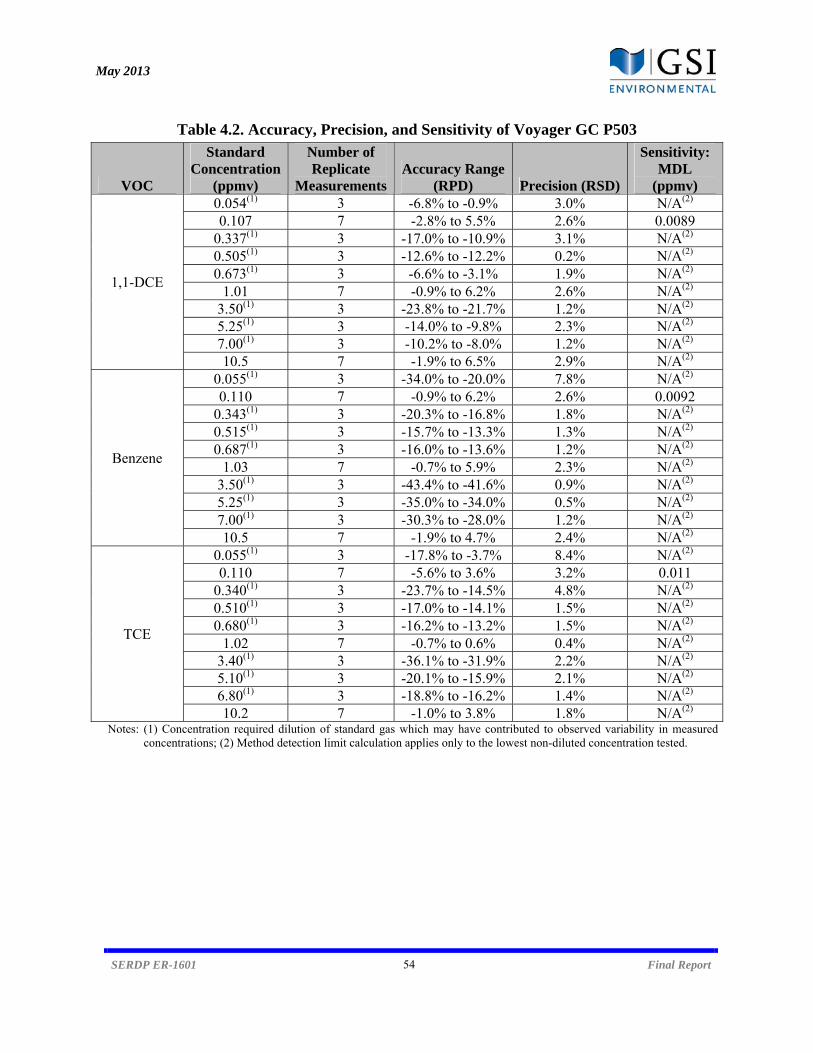
May 2013
SERDP ER-1601 54 Final Report
Table 4.2. Accuracy, Precision, and Sensitivity of Voyager GC P503
VOC
Standard Concentration
(ppmv)
Number of Replicate
MeasurementsAccuracy Range
(RPD) Precision (RSD)
Sensitivity: MDL
(ppmv)
1,1-DCE
0.054(1) 3 -6.8% to -0.9% 3.0% N/A(2)
0.107 7 -2.8% to 5.5% 2.6% 0.0089 0.337(1) 3 -17.0% to -10.9% 3.1% N/A(2) 0.505(1) 3 -12.6% to -12.2% 0.2% N/A(2) 0.673(1) 3 -6.6% to -3.1% 1.9% N/A(2)
1.01 7 -0.9% to 6.2% 2.6% N/A(2) 3.50(1) 3 -23.8% to -21.7% 1.2% N/A(2) 5.25(1) 3 -14.0% to -9.8% 2.3% N/A(2) 7.00(1) 3 -10.2% to -8.0% 1.2% N/A(2) 10.5 7 -1.9% to 6.5% 2.9% N/A(2)
Benzene
0.055(1) 3 -34.0% to -20.0% 7.8% N/A(2) 0.110 7 -0.9% to 6.2% 2.6% 0.0092
0.343(1) 3 -20.3% to -16.8% 1.8% N/A(2) 0.515(1) 3 -15.7% to -13.3% 1.3% N/A(2) 0.687(1) 3 -16.0% to -13.6% 1.2% N/A(2)
1.03 7 -0.7% to 5.9% 2.3% N/A(2) 3.50(1) 3 -43.4% to -41.6% 0.9% N/A(2) 5.25(1) 3 -35.0% to -34.0% 0.5% N/A(2) 7.00(1) 3 -30.3% to -28.0% 1.2% N/A(2) 10.5 7 -1.9% to 4.7% 2.4% N/A(2)
TCE
0.055(1) 3 -17.8% to -3.7% 8.4% N/A(2) 0.110 7 -5.6% to 3.6% 3.2% 0.011
0.340(1) 3 -23.7% to -14.5% 4.8% N/A(2) 0.510(1) 3 -17.0% to -14.1% 1.5% N/A(2) 0.680(1) 3 -16.2% to -13.2% 1.5% N/A(2)
1.02 7 -0.7% to 0.6% 0.4% N/A(2) 3.40(1) 3 -36.1% to -31.9% 2.2% N/A(2) 5.10(1) 3 -20.1% to -15.9% 2.1% N/A(2) 6.80(1) 3 -18.8% to -16.2% 1.4% N/A(2) 10.2 7 -1.0% to 3.8% 1.8% N/A(2)
Notes: (1) Concentration required dilution of standard gas which may have contributed to observed variability in measured concentrations; (2) Method detection limit calculation applies only to the lowest non-diluted concentration tested.

May 2013
SERDP ER-1601 55 Final Report
Table 4.3. Accuracy, Precision, and Sensitivity of Voyager GC P505
VOC
Standard Concentration
(ppmv)
Number of Replicate
Measurements Accuracy
Range (RPD) Precision (RSD) Sensitivity:
MDL (ppmv)
1,1-DCE 0.107 7 -7.8% to 4.6% 4.7% 0.0159 1.01 7 -5.6% to 1.8% 2.7% N/A(1) 10.5 7 -4.9% to 10.5% 1.8% N/A(1)
Benzene 0.110 7 -2.8% to 2.7% 1.9% 0.0065 1.03 7 -4.9% to 1.1% 2.4% N/A(1) 10.5 7 -6.8% to 10.5% 2.5% N/A(1)
TCE 0.110 7 -8.5% to 8.7% 5.9% 0.0209 1.02 7 -4.7% to 2.4% 2.8% N/A(1) 10.2 7 -7.7% to 10.2% 3.0% N/A(1)
Notes: (1) Method detection limit calculation applies only to the lowest non-diluted concentration tested. Finding: The Voyager GCs achieved the accuracy criteria for 94% of measurements and the precision criteria for 100%. For each of the three VOCs, the instrument MDL corresponds to a water-phase concentration of less than 0.5 g/L, less than the MCL of 5 to 7 g/L. Based on these results, the Voyager GCs was retained for the field portion of the study. 4.1.2 Headspace Sampling Method Validation Results The ability of the field GC to determine the VOC concentration in water through the measurement of headspace VOC concentration was evaluated with a series of partitioning experiments. An initial experiment to determine the time required for equilibration found that equilibrium partitioning between the water and air phases occurred in less than 100 minutes (see Figure 4.1). Based on this finding, subsequent experiments used an equilibration time of 100 minutes or more.
Figure 4.1. VOC Concentration vs. Time in Headspace of Equilibration Reactor.
0.0
0.5
1.0
1.5
2.0
2.5
3.0
3.5
4.0
0 50 100 150 200 250 300 350 400 450
Equilibration Time (minutes)
Hea
dsp
ace
Co
nce
ntr
atio
n (
ug
/L)
DCE
TCE
Benzene
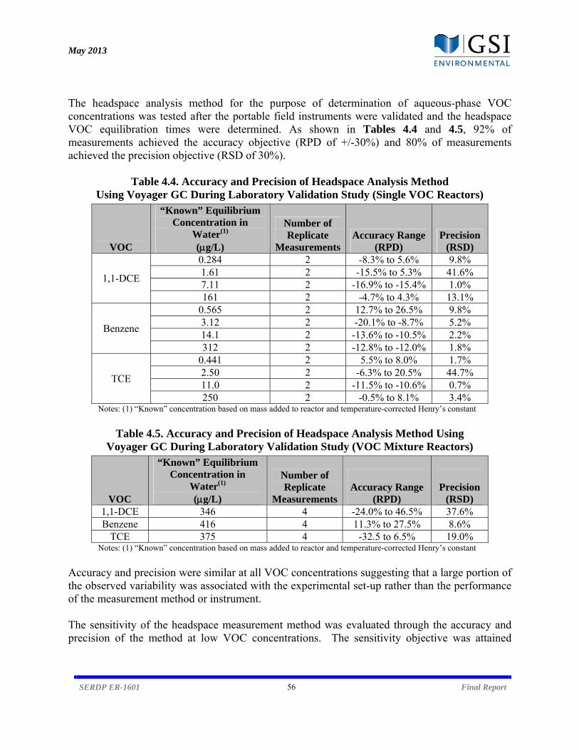
May 2013
SERDP ER-1601 56 Final Report
The headspace analysis method for the purpose of determination of aqueous-phase VOC concentrations was tested after the portable field instruments were validated and the headspace VOC equilibration times were determined. As shown in Tables 4.4 and 4.5, 92% of measurements achieved the accuracy objective (RPD of +/-30%) and 80% of measurements achieved the precision objective (RSD of 30%).
Table 4.4. Accuracy and Precision of Headspace Analysis Method Using Voyager GC During Laboratory Validation Study (Single VOC Reactors)
VOC
“Known” Equilibrium Concentration in
Water(1) (g/L)
Number of Replicate
MeasurementsAccuracy Range
(RPD) Precision
(RSD)
1,1-DCE
0.284 2 -8.3% to 5.6% 9.8% 1.61 2 -15.5% to 5.3% 41.6% 7.11 2 -16.9% to -15.4% 1.0% 161 2 -4.7% to 4.3% 13.1%
Benzene
0.565 2 12.7% to 26.5% 9.8% 3.12 2 -20.1% to -8.7% 5.2% 14.1 2 -13.6% to -10.5% 2.2% 312 2 -12.8% to -12.0% 1.8%
TCE
0.441 2 5.5% to 8.0% 1.7% 2.50 2 -6.3% to 20.5% 44.7% 11.0 2 -11.5% to -10.6% 0.7% 250 2 -0.5% to 8.1% 3.4%
Notes: (1) “Known” concentration based on mass added to reactor and temperature-corrected Henry’s constant
Table 4.5. Accuracy and Precision of Headspace Analysis Method Using
Voyager GC During Laboratory Validation Study (VOC Mixture Reactors)
VOC
“Known” Equilibrium Concentration in
Water(1) (g/L)
Number of Replicate
Measurements
Accuracy Range
(RPD)
Precision
(RSD) 1,1-DCE 346 4 -24.0% to 46.5% 37.6% Benzene 416 4 11.3% to 27.5% 8.6%
TCE 375 4 -32.5 to 6.5% 19.0% Notes: (1) “Known” concentration based on mass added to reactor and temperature-corrected Henry’s constant
Accuracy and precision were similar at all VOC concentrations suggesting that a large portion of the observed variability was associated with the experimental set-up rather than the performance of the measurement method or instrument. The sensitivity of the headspace measurement method was evaluated through the accuracy and precision of the method at low VOC concentrations. The sensitivity objective was attained
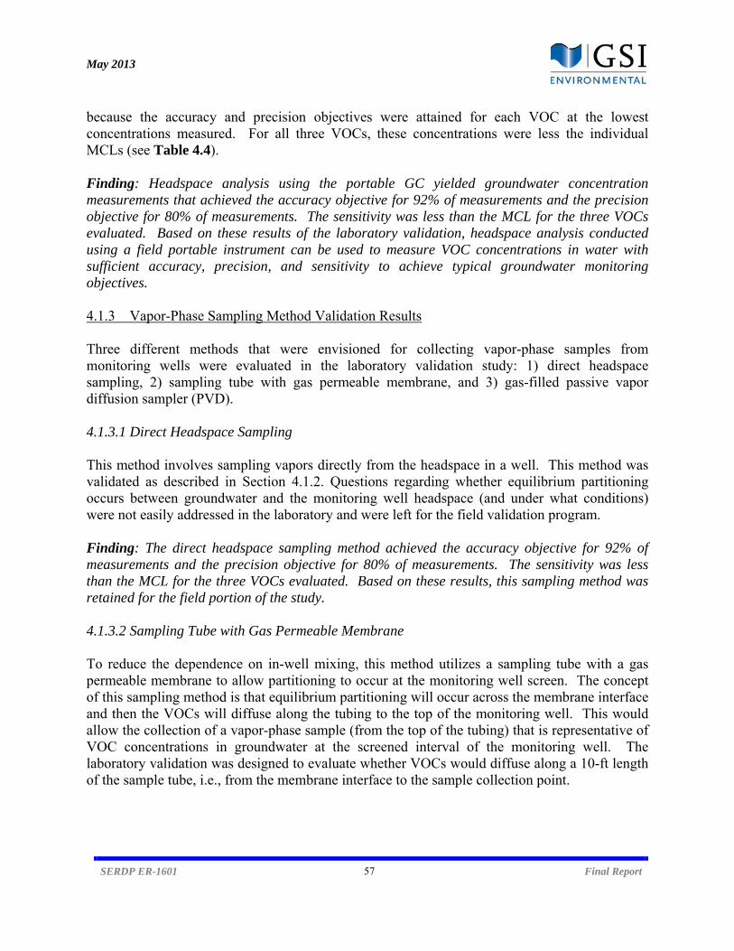
May 2013
SERDP ER-1601 57 Final Report
because the accuracy and precision objectives were attained for each VOC at the lowest concentrations measured. For all three VOCs, these concentrations were less the individual MCLs (see Table 4.4). Finding: Headspace analysis using the portable GC yielded groundwater concentration measurements that achieved the accuracy objective for 92% of measurements and the precision objective for 80% of measurements. The sensitivity was less than the MCL for the three VOCs evaluated. Based on these results of the laboratory validation, headspace analysis conducted using a field portable instrument can be used to measure VOC concentrations in water with sufficient accuracy, precision, and sensitivity to achieve typical groundwater monitoring objectives. 4.1.3 Vapor-Phase Sampling Method Validation Results Three different methods that were envisioned for collecting vapor-phase samples from monitoring wells were evaluated in the laboratory validation study: 1) direct headspace sampling, 2) sampling tube with gas permeable membrane, and 3) gas-filled passive vapor diffusion sampler (PVD). 4.1.3.1 Direct Headspace Sampling This method involves sampling vapors directly from the headspace in a well. This method was validated as described in Section 4.1.2. Questions regarding whether equilibrium partitioning occurs between groundwater and the monitoring well headspace (and under what conditions) were not easily addressed in the laboratory and were left for the field validation program. Finding: The direct headspace sampling method achieved the accuracy objective for 92% of measurements and the precision objective for 80% of measurements. The sensitivity was less than the MCL for the three VOCs evaluated. Based on these results, this sampling method was retained for the field portion of the study. 4.1.3.2 Sampling Tube with Gas Permeable Membrane To reduce the dependence on in-well mixing, this method utilizes a sampling tube with a gas permeable membrane to allow partitioning to occur at the monitoring well screen. The concept of this sampling method is that equilibrium partitioning will occur across the membrane interface and then the VOCs will diffuse along the tubing to the top of the monitoring well. This would allow the collection of a vapor-phase sample (from the top of the tubing) that is representative of VOC concentrations in groundwater at the screened interval of the monitoring well. The laboratory validation was designed to evaluate whether VOCs would diffuse along a 10-ft length of the sample tube, i.e., from the membrane interface to the sample collection point.
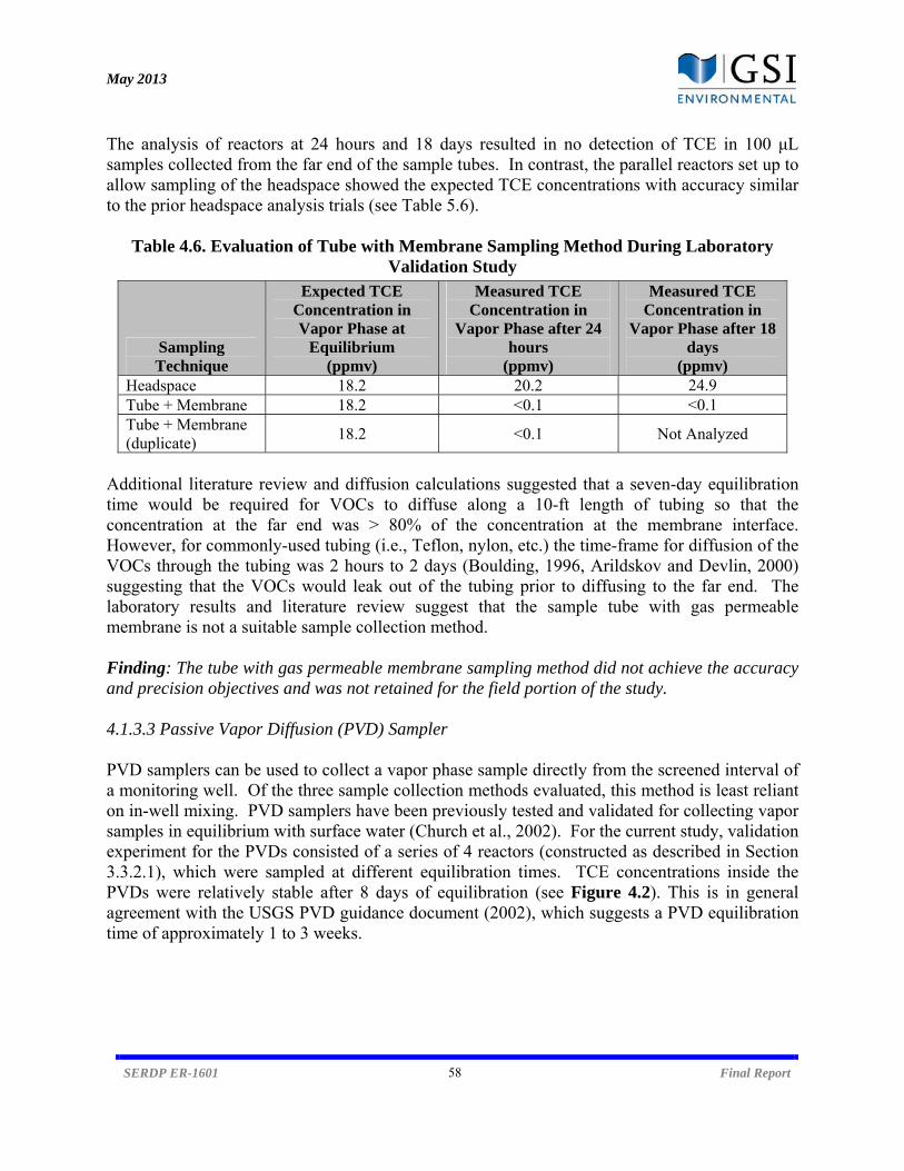
May 2013
SERDP ER-1601 58 Final Report
The analysis of reactors at 24 hours and 18 days resulted in no detection of TCE in 100 μL samples collected from the far end of the sample tubes. In contrast, the parallel reactors set up to allow sampling of the headspace showed the expected TCE concentrations with accuracy similar to the prior headspace analysis trials (see Table 5.6).
Table 4.6. Evaluation of Tube with Membrane Sampling Method During Laboratory Validation Study
Sampling Technique
Expected TCE Concentration in Vapor Phase at
Equilibrium (ppmv)
Measured TCE Concentration in
Vapor Phase after 24 hours
(ppmv)
Measured TCE Concentration in
Vapor Phase after 18 days
(ppmv) Headspace 18.2 20.2 24.9 Tube + Membrane 18.2 <0.1 <0.1 Tube + Membrane (duplicate) 18.2 <0.1 Not Analyzed
Additional literature review and diffusion calculations suggested that a seven-day equilibration time would be required for VOCs to diffuse along a 10-ft length of tubing so that the concentration at the far end was > 80% of the concentration at the membrane interface. However, for commonly-used tubing (i.e., Teflon, nylon, etc.) the time-frame for diffusion of the VOCs through the tubing was 2 hours to 2 days (Boulding, 1996, Arildskov and Devlin, 2000) suggesting that the VOCs would leak out of the tubing prior to diffusing to the far end. The laboratory results and literature review suggest that the sample tube with gas permeable membrane is not a suitable sample collection method. Finding: The tube with gas permeable membrane sampling method did not achieve the accuracy and precision objectives and was not retained for the field portion of the study. 4.1.3.3 Passive Vapor Diffusion (PVD) Sampler PVD samplers can be used to collect a vapor phase sample directly from the screened interval of a monitoring well. Of the three sample collection methods evaluated, this method is least reliant on in-well mixing. PVD samplers have been previously tested and validated for collecting vapor samples in equilibrium with surface water (Church et al., 2002). For the current study, validation experiment for the PVDs consisted of a series of 4 reactors (constructed as described in Section 3.3.2.1), which were sampled at different equilibration times. TCE concentrations inside the PVDs were relatively stable after 8 days of equilibration (see Figure 4.2). This is in general agreement with the USGS PVD guidance document (2002), which suggests a PVD equilibration time of approximately 1 to 3 weeks.
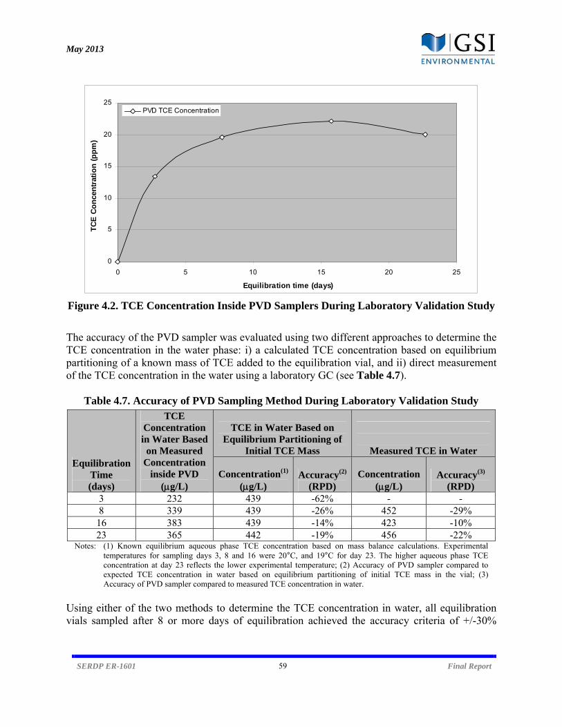
May 2013
SERDP ER-1601 59 Final Report
Figure 4.2. TCE Concentration Inside PVD Samplers During Laboratory Validation Study
The accuracy of the PVD sampler was evaluated using two different approaches to determine the TCE concentration in the water phase: i) a calculated TCE concentration based on equilibrium partitioning of a known mass of TCE added to the equilibration vial, and ii) direct measurement of the TCE concentration in the water using a laboratory GC (see Table 4.7).
Table 4.7. Accuracy of PVD Sampling Method During Laboratory Validation Study
Equilibration Time (days)
TCE Concentration in Water Based
on Measured Concentration
inside PVD (g/L)
TCE in Water Based on
Equilibrium Partitioning of Initial TCE Mass
Measured TCE in Water
Concentration(1) (g/L)
Accuracy(2) (RPD)
Concentration (g/L)
Accuracy(3) (RPD)
3 232 439 -62% - - 8 339 439 -26% 452 -29%
16 383 439 -14% 423 -10% 23 365 442 -19% 456 -22%
Notes: (1) Known equilibrium aqueous phase TCE concentration based on mass balance calculations. Experimental temperatures for sampling days 3, 8 and 16 were 20°C, and 19°C for day 23. The higher aqueous phase TCE concentration at day 23 reflects the lower experimental temperature; (2) Accuracy of PVD sampler compared to expected TCE concentration in water based on equilibrium partitioning of initial TCE mass in the vial; (3) Accuracy of PVD sampler compared to measured TCE concentration in water.
Using either of the two methods to determine the TCE concentration in water, all equilibration vials sampled after 8 or more days of equilibration achieved the accuracy criteria of +/-30%
0
5
10
15
20
25
0 5 10 15 20 25
Equilibration time (days)
TC
E C
on
cen
trat
ion
(p
pm
)
PVD TCE Concentration

May 2013
SERDP ER-1601 60 Final Report
RPD. Although the replicate vials were not analyzed on the same day, precision was evaluated by calculating the RSD for the three vials analyzed after the TCE concentration inside the PVDs had stabilized (i.e., days 8, 16, and 23). The RSD (between the water phase TCE concentrations determined from the measured TCE concentrations inside the PVDs) for these three vials was 6.2%, below the 30% objective. The results from this limited laboratory validation support the previous work done by the USGS that demonstrated by suitability of PVD samplers for measuring VOC concentrations in water. Finding: The PVD sampling method achieved the accuracy and precision objectives for 100% of measurements and was retained for the field portion of the study. 4.2 Temperature Study Vertical temperature gradients and effect on volatile organic compound (VOC) concentrations measured by low flow and passive diffusion bag samples were evaluated as part of a limited field program at two shallow monitoring wells. The results were used to understand the potential effect on concentrations estimated using the vapor-phase based approach, as well as to help design appropriate sampling strategies. 4.2.1 Temperature Data Temperatures were recorded hourly at four elevations at each well for the period from December 2008 to April 2010 (Figure 4.3). Some gaps in the temperature measurements occurred due to i) failure to download temperature readings from 17 January 2009 to 7 March 2009 before they were overwritten by more recent measurements, ii) failure of individual iButton at various times, and iii) removal of the iButtons from the wells from during various periods to allow installation of passive diffusion samplers and other equipment. In both wells, the largest seasonal variation in temperature was observed at the shallowest elevation. Less seasonal variation was observed at the deeper elevations and at these elevations, the maximum and minimum temperatures occurred later in the season.

May 2013
SERDP ER-1601 61 Final Report
Figure 4.3. Measured and Predicted Groundwater Temperature Over Monitoring Period During Temperature Study. Y-axis shows temperature (degrees Celsius). Blue diamonds show measured groundwater temperatures and green lines show predicted temperatures using model (Hillel, 1982) and input values listed in Section 3.2. The soil temperature model described in Section 3.2 (Hillel, 1982) was used to generate temperature predictions based on well and environmental conditions. These data are also shown in Figure 4.3, and demonstrate that the measured groundwater temperature patterns in both wells were generally consistent with the predicted soil temperature profiles in terms of both magnitudes of temperature variation and timing of observed minimum and maximum temperatures. At depths greater than 6 m, the model-predicted magnitude of temperature variation matched the observations, but the maximum temperature occurred earlier than predicted. This comparison indicates that a simple model of soil temperature model can be used to estimate the approximate time and depth intervals during which the groundwater within study wells were expected to exhibit thermal convective mixing or thermally-induced stratification. 4.2.2 VOC Concentration Data In order to characterize the vertical distribution of VOCs within the two wells, groundwater concentrations were measured in November 2009 and May 2010 at same four elevations using passive diffusion samplers and at the lowest elevation using low flow sampling. The November 2009 event was scheduled during a period which is consistent with “late summer” conditions for the region (Houston), when the target sampling intervals were expected to be thermally stabilized. The May 2010 event was scheduled during a period which is consistent with “late
17
19
21
23
25
27
29
Jun‐08
Dec‐0
8
Jul‐0
9
Jan‐10
Aug‐1
0
MW‐51 (2.7 m)
17
19
21
23
25
27
29
Jun‐08
Dec‐0
8
Jul‐0
9
Jan‐10
Aug‐1
0
MW‐51 (3.5 m)
17
19
21
23
25
27
29
Jun‐08
Dec‐0
8
Jul‐0
9
Jan‐10
Aug‐1
0
MW‐51 (4.4 m)
17
19
21
23
25
27
29
Jun‐08
Dec‐0
8
Jul‐0
9
Jan‐10
Aug‐1
0
MW‐51 (5.4 m)
19
20
21
22
23
24
25
26
27
Jun‐08
Dec‐0
8
Jul‐0
9
Jan‐10
Aug‐1
0
MW‐53 (4.2 m)
19
20
21
22
23
24
25
26
27
Jun‐08
Dec‐0
8
Jul‐0
9
Jan‐10
Aug‐1
0
MW‐53 (6.3 m)
19
20
21
22
23
24
25
26
27
Jun‐08
Dec‐0
8
Jul‐0
9
Jan‐10
Aug‐1
0
MW‐53 (8.3 m)
19
20
21
22
23
24
25
26
27
Jun‐08
Dec‐0
8
Jul‐0
9
Jan‐10
Aug‐1
0
MW‐53 (10.4 m)
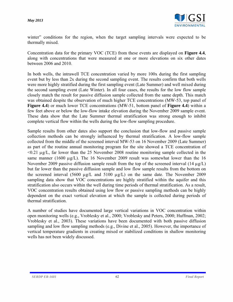
May 2013
SERDP ER-1601 62 Final Report
winter” conditions for the region, when the target sampling intervals were expected to be thermally mixed. Concentration data for the primary VOC (TCE) from these events are displayed on Figure 4.4, along with concentrations that were measured at one or more elevations on six other dates between 2006 and 2010. In both wells, the intrawell TCE concentration varied by more 100x during the first sampling event but by less than 2x during the second sampling event. The results confirm that both wells were more highly stratified during the first sampling event (Late Summer) and well mixed during the second sampling event (Late Winter). In all four cases, the results for the low flow sample closely match the result for passive diffusion sample collected from the same depth. This match was obtained despite the observation of much higher TCE concentrations (MW-53, top panel of Figure 4.4) or much lower TCE concentrations (MW-51, bottom panel of Figure 4.4) within a few feet above or below the low-flow intake elevation during the November 2009 sample event. These data show that the Late Summer thermal stratification was strong enough to inhibit complete vertical flow within the wells during the low-flow sampling procedure. Sample results from other dates also support the conclusion that low-flow and passive sample collection methods can be strongly influenced by thermal stratification. A low-flow sample collected from the middle of the screened interval MW-53 on 16 November 2009 (Late Summer) as part of the routine annual monitoring program for the site showed a TCE concentration of <0.21 g/L, far lower than the 25 November 2008 routine monitoring sample collected in the same manner (1600 g/L). The 16 November 2009 result was somewhat lower than the 16 November 2009 passive diffusion sample result from the top of the screened interval (14 g/L) but far lower than the passive diffusion sample and low flow sample results from the bottom on the screened interval (5600 g/L and 5100 g/L) on the same date. The November 2009 sampling data show that VOC concentrations are highly stratified within the aquifer and this stratification also occurs within the well during time periods of thermal stratification. As a result, VOC concentration results obtained using low flow or passive sampling methods can be highly dependent on the exact vertical elevation at which the sample is collected during periods of thermal stratification. A number of studies have documented large vertical variations in VOC concentration within open monitoring wells (e.g., Vroblesky et al., 2000; Vroblesky and Peters, 2000; Huffman, 2002; Vroblesky et al., 2003). These variations have been documented with both passive diffusion sampling and low flow sampling methods (e.g., Divine et al., 2005). However, the importance of vertical temperature gradients in creating mixed or stabilized conditions in shallow monitoring wells has not been widely discussed.
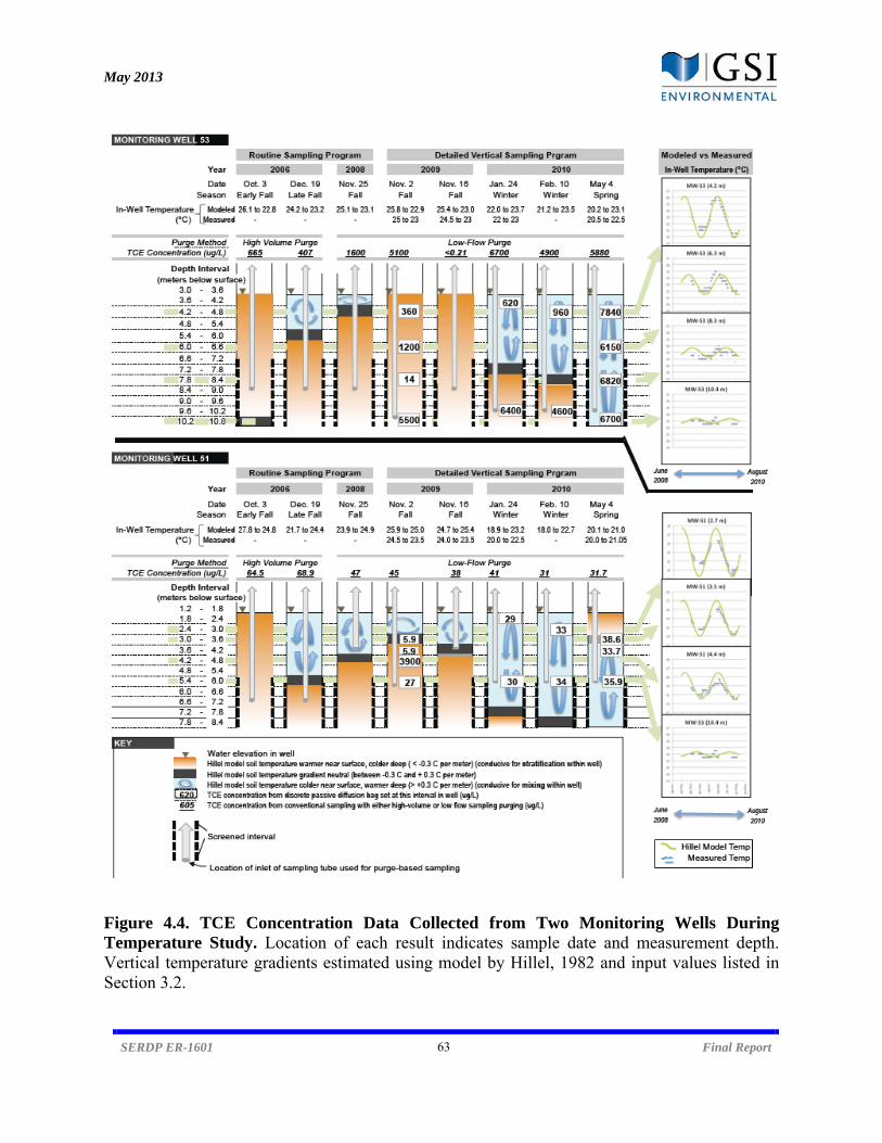
May 2013
SERDP ER-1601 63 Final Report
Figure 4.4. TCE Concentration Data Collected from Two Monitoring Wells During Temperature Study. Location of each result indicates sample date and measurement depth. Vertical temperature gradients estimated using model by Hillel, 1982 and input values listed in Section 3.2.
May 2013
SERDP ER-1601 64 Final Report
Theoretical considerations and site data suggest vertical temperature gradients within shallow aquifers can have a significant effect on groundwater monitoring results obtained using low flow and passive sampling methods. Other researchers have evaluated the impact of temperature gradients on oxygen transport within a monitoring well (Vroblesky et al., 2007) and mixing of water from above and within the screened interval during the low flow purging process (Martin-Hayden, 2000). However, we are not aware of any studies on effect of temperature gradients on stratification in VOC concentrations within a monitoring well. In fact, out of 11 studies we reviewed that have used passive diffusion samplers to determine vertical VOC concentration gradients, none consider the effect of vertical temperature gradients on well dynamics. Temperature gradients of less than 0.01°C per meter (0.003°C per foot) that increase with depth are sufficient to support thermal convection resulting in mixing between depths within monitoring wells (Sammel, 1968). When temperature gradients are reversed so that temperatures decrease with depth (e.g., in Late Summer), the resulting density gradient will inhibit mixing within the well. In the absence of other forces such as naturally occurring hydrogeologic vertical gradients driving vertical flow, the thermal stratification will result in constituent concentration profiles within a monitoring well that are similar to those within the adjacent aquifer. When constituent concentrations are stratified, then the results obtained by passive or low flow sample collection methods will be highly dependent on the depth at which the sample is collected. In the absence of vertical pressure gradients within the screened portion of the aquifer, low flow sampling is commonly assumed to draw water from the entire screened interval of the well yielding a flow-weighted average sample (Varljen et al., 2006). However, under thermally stabilized conditions (typically expected in late Summer and early Fall), the resulting density gradient inhibits the vertical flow of water within the well (and in the adjacent aquifer), narrowing the interval from which water is obtained. Because both low flow and passive sampling methods are extremely sensitive to thermal stratification in shallow monitoring wells, the results obtained using these sampling methods will potentially be significantly more variable than those obtained using high volume purge methods. Proper consideration of the effects of temperature gradients on well dynamics provides a previously unrecognized opportunity to gain additional information from traditional monitoring wells. During time periods of thermal mixing, a sample collected using low flow or passive methods will provide a flow-weighted average concentration for the screened interval. In contrast, during periods of thermal stratification, samples collected from different depths within the open monitoring well can be used to characterize the degree of concentration stratification within the aquifer. Figure 4.5 shows temperature gradients and predicted mixing conditions as a function of season and depth for a variety of climates (e.g., Houston, TX and San Francisco, CA). The temperature gradients were calculated using the soil temperature model and input values described in Section 3.2 except that A0 was 7.5°C for San Francisco. Low-flow or no-purge samples collected from traditional monitoring wells during periods of strong thermal mixing should be representative of flow-weighted conditions within the aquifer regardless of the specific sample depth within the screened interval of the well. Low-flow or no-purge samples
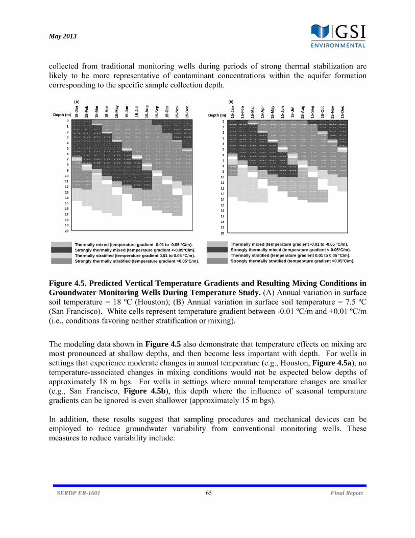
May 2013
SERDP ER-1601 65 Final Report
collected from traditional monitoring wells during periods of strong thermal stabilization are likely to be more representative of contaminant concentrations within the aquifer formation corresponding to the specific sample collection depth.
Figure 4.5. Predicted Vertical Temperature Gradients and Resulting Mixing Conditions in Groundwater Monitoring Wells During Temperature Study. (A) Annual variation in surface soil temperature = 18 ºC (Houston); (B) Annual variation in surface soil temperature = 7.5 ºC (San Francisco). White cells represent temperature gradient between -0.01 ºC/m and +0.01 ºC/m (i.e., conditions favoring neither stratification or mixing).
The modeling data shown in Figure 4.5 also demonstrate that temperature effects on mixing are most pronounced at shallow depths, and then become less important with depth. For wells in settings that experience moderate changes in annual temperature (e.g., Houston, Figure 4.5a), no temperature-associated changes in mixing conditions would not be expected below depths of approximately 18 m bgs. For wells in settings where annual temperature changes are smaller (e.g., San Francisco, Figure 4.5b), this depth where the influence of seasonal temperature gradients can be ignored is even shallower (approximately 15 m bgs). In addition, these results suggest that sampling procedures and mechanical devices can be employed to reduce groundwater variability from conventional monitoring wells. These measures to reduce variability include:
(A)
Depth (m) 15
-Jan
15-F
eb
15-M
ar
15-A
pr
15-M
ay
15-J
un
15-J
ul
15-A
ug
15-S
ep
15-O
ct
15-N
ov
15-D
ec
2.77 0.85 1.1 3 4 3.9 2.9 0.9 1.22 3 4.01 3.932.89 1.13 0.7 2.6 3.7 3.8 3 1.2 0.84 2.62 3.75 3.842.85 1.34 0.4 2.1 3.3 3.6 2.9 1.4 0.46 2.16 3.32 3.572.78 1.49 0 1.7 2.9 3.3 2.8 1.6 0.13 1.74 2.92 3.292.68 1.59 0.22 1.3 2.5 3 2.7 1.7 0.1 1.36 2.54 3.022.55 1.66 0.45 1 2.1 2.7 2.6 1.7 0.4 1.03 2.19 2.742.42 1.69 0.63 0.7 1.8 2.5 2.4 1.7 0.6 0.73 1.86 2.472.27 1.7 0.77 0.5 1.5 2.2 2.3 1.7 0.7 0.47 1.56 2.212.19 1.74 0.91 0.2 1.3 2 2.2 1.8 0.9 0.26 1.34 2.031.94 1.63 0.96 0 1 1.7 1.9 1.7 0.9 0.05 1.03 1.711.78 1.57 1.01 0.12 0.8 1.5 1.8 1.6 1 0.1 0.81 1.491.61 1.5 1.04 0.26 0.6 1.3 1.6 1.5 1 0.2 0.61 1.281.46 1.42 1.05 0.36 0.4 1.1 1.4 1.4 1 0.4 0.44 1.081.3 1.33 1.04 0.45 0.2 0.9 1.3 1.3 1 0.4 0.28 0.911.15 1.24 1.02 0.51 0.1 0.7 1.1 1.2 1 0.5 0.15 0.751.01 1.15 0.99 0.56 0 0.6 1 1.1 1 0.5 0.04 0.60.88 1.05 0.95 0.59 0.08 0.5 0.9 1 0.9 0.6 0.1 0.470.76 0.96 0.9 0.61 0.16 0.3 0.7 1 0.9 0.6 0.1 0.350.65 0.86 0.85 0.62 0.22 0.2 0.6 0.9 0.8 0.6 0.2 0.250.54 0.77 0.8 0.61 0.27 0.2 0.5 0.8 0.8 0.6 0.3 0.160.45 0.68 0.74 0.6 0.31 0.1 0.4 0.7 0.7 0.6 0.3 0.080.36 0.6 0.68 0.58 0.34 0 0.3 0.6 0.7 0.6 0.3 0.020.28 0.52 0.62 0.56 0.35 0.05 0.3 0.5 0.6 0.6 0.3 00.21 0.45 0.56 0.53 0.36 0.09 0.2 0.4 0.6 0.5 0.4 0.10.15 0.38 0.5 0.5 0.37 0.13 0.1 0.4 0.5 0.5 0.4 0.10.1 0.32 0.45 0.47 0.36 0.16 0.1 0.3 0.5 0.5 0.4 0.20.05 0.27 0.4 0.44 0.36 0.18 0 0.3 0.4 0.4 0.4 0.20.01 0.22 0.35 0.4 0.35 0.2 0 0.2 0.4 0.4 0.3 0.20 0.17 0.3 0.37 0.33 0.21 0.03 0.2 0.3 0.4 0.3 0.20 0.13 0.26 0.33 0.32 0.21 0.06 0.1 0.3 0.3 0.3 0.20.1 0.09 0.22 0.3 0.3 0.22 0.08 0.1 0.2 0.3 0.3 0.20.1 0.06 0.18 0.27 0.28 0.21 0.1 0.1 0.2 0.3 0.3 0.20.1 0.03 0.15 0.24 0.26 0.21 0.11 0 0.2 0.2 0.3 0.20.1 0.01 0.12 0.21 0.24 0.2 0.12 0 0.1 0.2 0.2 0.20.1 0 0.09 0.18 0.22 0.2 0.12 0.02 0.1 0.2 0.2 0.20.1 0 0.07 0.15 0.2 0.19 0.13 0.03 0.1 0.2 0.2 0.20. 0 0.05 0. 3 0. 8 0. 8 0. 3 0.05 0. 0. 0. 0.0.1 0.1 0.03 0.11 0.16 0.16 0.13 0.06 0 0.1 0.2 0.20.1 0.1 0.01 0.09 0.14 0.15 0.13 0.06 0 0.1 0.1 0.20. 0. 0 0.07 0. 0. 4 0. 0.07 0 0. 0. 0.0.1 0.1 0 0.06 0.11 0.13 0.12 0.07 0.01 0.1 0.1 0.10.1 0.1 0 0.04 0.09 0.12 0.11 0.07 0.02 0 0.1 0.10. 0. 0 0.03 0.08 0. 0. 0.08 0.03 0 0. 0.0.1 0.1 0 0.02 0.06 0.09 0.1 0.08 0.03 0 0.1 0.10.1 0.1 0 0.01 0.05 0.08 0.09 0.07 0.04 0 0.1 0.10. 0. 0 0 0.04 0.07 0.08 0.07 0.04 0 0 0.0.1 0.1 0 0 0.03 0.06 0.08 0.07 0.04 0.01 0 0.10.1 0.1 0 0 0.02 0.05 0.07 0.07 0.04 0.01 0 0.10. 0. 0 0 0.0 0.05 0.06 0.06 0.04 0.0 0 00. 0. 0 0 0.0 0.04 0.06 0.06 0.04 0.0 0 00 0.1 0 0 0 0.03 0.05 0.05 0.04 0.02 0 00 0 0 0 0 0.03 0.04 0.05 0.04 0.0 0 00 0 0 0 0 0.0 0.04 0.05 0.04 0.03 0 00 0 0 0 0 0.01 0.03 0.04 0.04 0.03 0.01 00 0 0 0 0 0.0 0.03 0.04 0.04 0.03 0.0 00 0 0 0 0 0.0 0.0 0.03 0.03 0.03 0.0 00 0 0 0 0 0 0.02 0.03 0.03 0.03 0.01 00 0 0 0 0 0 0.01 0.03 0.03 0.03 0.01 00 0 0 0 0 0 0.0 0.0 0.03 0.0 0.0 00 0 0 0 0 0 0.01 0.02 0.02 0.02 0.02 00 0 0 0 0 0 0.01 0.02 0.02 0.02 0.02 0.010 0 0 0 0 0 0 0.0 0.0 0.0 0.0 0.00 0 0 0 0 0 0 0.01 0.02 0.02 0.02 0.010 0 0 0 0 0 0 0.01 0.02 0.02 0.02 0.010 0 0 0 0 0 0 0.0 0.0 0.0 0.0 0.00 0 0 0 0 0 0 0.01 0.01 0.01 0.01 0.010 0 0 0 0 0 0 0 0.01 0.01 0.01 0.010 0 0 0 0 0 0 0 0.0 0.0 0.0 0.00 0 0 0 0 0 0 0 0.01 0.01 0.01 0.010.01 0 0 0 0 0 0 0 0.01 0.01 0.01 0.010.0 0 0 0 0 0 0 0 0 0.0 0.0 0.00.01 0 0 0 0 0 0 0 0 0.01 0.01 0.010.01 0 0 0 0 0 0 0 0 0.01 0.01 0.010.0 0 0 0 0 0 0 0 0 0.0 0.0 0.00.01 0 0 0 0 0 0 0 0 0 0.01 0.010.01 0 0 0 0 0 0 0 0 0 0.01 0.010.0 0 0 0 0 0 0 0 0 0 0.0 0.00.01 0 0 0 0 0 0 0 0 0 0 0.010 0 0 0 0 0 0 0 0 0 0 00 0 0 0 0 0 0 0 0 0 0 0
Thermally mixed (temperature gradient -0.01 to -0.05 °C/m). Strongly thermally mixed (temperature gradient <-0.05°C/m). Thermally stratified (temperature gradient 0.01 to 0.05 °C/m). Strongly thermally stratified (temperature gradient >0.05°C/m).
17
18
19
14
15
16
11
12
13
8
9
10
5
6
7
0
20
1
2
3
4
(B)
Depth (m) 15
-Jan
15-F
eb
15-M
ar
15-A
pr
15-M
ay
15-J
un
15-J
ul
15-A
ug
15-S
ep
15-O
ct
15-N
ov
15-D
ec
1.26 0.5 0.3 1.1 1.6 1.7 1.3 0.5 0.36 1.14 1.63 1.671.3 0.61 0.2 1 1.5 1.6 1.3 0.6 0.21 0.98 1.51 1.621.26 0.68 0 0.8 1.3 1.5 1.3 0.7 0.06 0.79 1.33 1.51.22 0.72 0.1 0.6 1.1 1.4 1.2 0.8 0.1 0.62 1.16 1.371.16 0.75 0.2 0.5 1 1.2 1.2 0.8 0.2 0.47 1 1.251.1 0.77 0.28 0.3 0.8 1.1 1.1 0.8 0.3 0.33 0.85 1.121.03 0.77 0.35 0.2 0.7 1 1 0.8 0.3 0.22 0.71 10.96 0.76 0.4 0.1 0.6 0.9 1 0.8 0.4 0.12 0.59 0.890.92 0.77 0.45 0 0.5 0.8 0.9 0.8 0.4 0.03 0.49 0.810.81 0.72 0.46 0.06 0.4 0.7 0.8 0.7 0.4 0 0.37 0.680.73 0.68 0.47 0.12 0.3 0.6 0.7 0.7 0.5 0.1 0.28 0.580.66 0.65 0.48 0.16 0.2 0.5 0.7 0.7 0.5 0.2 0.2 0.490.59 0.61 0.47 0.2 0.1 0.4 0.6 0.6 0.5 0.2 0.13 0.410.53 0.56 0.46 0.23 0.1 0.3 0.5 0.6 0.5 0.2 0.07 0.340.46 0.52 0.45 0.25 0 0.3 0.5 0.5 0.4 0.2 0.02 0.270.4 0.48 0.43 0.27 0.04 0.2 0.4 0.5 0.4 0.3 0 0.210.35 0.43 0.41 0.28 0.07 0.2 0.3 0.4 0.4 0.3 0.1 0.160.29 0.39 0.39 0.28 0.1 0.1 0.3 0.4 0.4 0.3 0.1 0.110.25 0.35 0.36 0.28 0.12 0.1 0.2 0.3 0.4 0.3 0.1 0.070.2 0.31 0.34 0.27 0.14 0 0.2 0.3 0.3 0.3 0.1 0.040.16 0.27 0.31 0.27 0.15 0 0.2 0.3 0.3 0.3 0.1 0.010.13 0.24 0.28 0.25 0.16 0.02 0.1 0.2 0.3 0.3 0.2 00.1 0.21 0.26 0.24 0.17 0.04 0.1 0.2 0.3 0.2 0.2 00.07 0.18 0.23 0.23 0.17 0.06 0.1 0.2 0.2 0.2 0.2 0.10.05 0.15 0.2 0.21 0.17 0.07 0 0.1 0.2 0.2 0.2 0.10.02 0.12 0.18 0.2 0.16 0.08 0 0.1 0.2 0.2 0.2 0.10.01 0.1 0.16 0.18 0.16 0.09 0 0.1 0.2 0.2 0.2 0.10 0.08 0.14 0.17 0.15 0.09 0.01 0.1 0.1 0.2 0.1 0.10 0.06 0.12 0.15 0.14 0.1 0.03 0.1 0.1 0.2 0.1 0.10 0.04 0.1 0.14 0.14 0.1 0.04 0 0.1 0.1 0.1 0.10 0.03 0.08 0.12 0.13 0.1 0.04 0 0.1 0.1 0.1 0.10 0.02 0.07 0.11 0.12 0.1 0.05 0 0.1 0.1 0.1 0.10.1 0 0.05 0.09 0.11 0.09 0.05 0 0.1 0.1 0.1 0.10.1 0 0.04 0.08 0.1 0.09 0.06 0.01 0 0.1 0.1 0.10.1 0 0.03 0.07 0.09 0.09 0.06 0.01 0 0.1 0.1 0.10.1 0 0.02 0.06 0.08 0.08 0.06 0.02 0 0.1 0.1 0.10.1 0 0.01 0.05 0.07 0.08 0.06 0.03 0 0.1 0.1 0.10.1 0 0.01 0.04 0.06 0.07 0.06 0.03 0 0 0.1 0.10.1 0 0 0.03 0.06 0.06 0.06 0.03 0 0 0.1 0.10.1 0 0 0.03 0.05 0.06 0.05 0.03 0 0 0 0.10.1 0 0 0.02 0.04 0.05 0.05 0.03 0.01 0 0 0.10 0 0 0.01 0.04 0.05 0.05 0.03 0.01 0 0 00 0 0 0.01 0.03 0.04 0.04 0.03 0.01 0 0 00 0 0 0 0.02 0.04 0.04 0.03 0.02 0 0 00 0 0 0 0.02 0.03 0.04 0.03 0.02 0 0 00 0 0 0 0.01 0.03 0.03 0.03 0.02 0 0 00 0 0 0 0.01 0.02 0.03 0.03 0.02 0.01 0 00 0 0 0 0.01 0.02 0.03 0.03 0.02 0.01 0 00 0 0 0 0.01 0.02 0.03 0.03 0.02 0.01 0 00 0 0 0 0 0.01 0.02 0.02 0.02 0.01 0 00 0 0 0 0 0.01 0.02 0.02 0.02 0.01 0 00 0 0 0 0 0.01 0.02 0.02 0.02 0.01 0 00 0 0 0 0 0.01 0.01 0.02 0.02 0.01 0 00 0 0 0 0 0 0.01 0.02 0.02 0.01 0 00 0 0 0 0 0 0.01 0.02 0.02 0.01 0.01 00 0 0 0 0 0 0.01 0.01 0.01 0.01 0.01 00 0 0 0 0 0 0.01 0.01 0.01 0.01 0.01 00 0 0 0 0 0 0.01 0.01 0.01 0.01 0.01 00 0 0 0 0 0 0 0.01 0.01 0.01 0.01 00 0 0 0 0 0 0 0.01 0.01 0.01 0.01 00 0 0 0 0 0 0 0.01 0.01 0.01 0.01 00 0 0 0 0 0 0 0.01 0.01 0.01 0.01 00 0 0 0 0 0 0 0 0.01 0.01 0.01 00 0 0 0 0 0 0 0 0.01 0.01 0.01 00 0 0 0 0 0 0 0 0.01 0.01 0.01 00 0 0 0 0 0 0 0 0 0.01 0.01 00 0 0 0 0 0 0 0 0 0.01 0.01 00 0 0 0 0 0 0 0 0 0.01 0.01 00 0 0 0 0 0 0 0 0 0 0.01 00 0 0 0 0 0 0 0 0 0 0 00 0 0 0 0 0 0 0 0 0 0 00 0 0 0 0 0 0 0 0 0 0 00 0 0 0 0 0 0 0 0 0 0 00 0 0 0 0 0 0 0 0 0 0 00 0 0 0 0 0 0 0 0 0 0 00 0 0 0 0 0 0 0 0 0 0 00 0 0 0 0 0 0 0 0 0 0 00 0 0 0 0 0 0 0 0 0 0 00 0 0 0 0 0 0 0 0 0 0 00 0 0 0 0 0 0 0 0 0 0 0
Thermally mixed (temperature gradient -0.01 to -0.05 °C/m). Strongly thermally mixed (temperature gradient <-0.05°C/m). Thermally stratified (temperature gradient 0.01 to 0.05 °C/m). Strongly thermally stratified (temperature gradient >0.05°C/m).
0
1
2
3
4
5
6
7
8
9
10
11
12
13
14
18
19
20
15
16
17
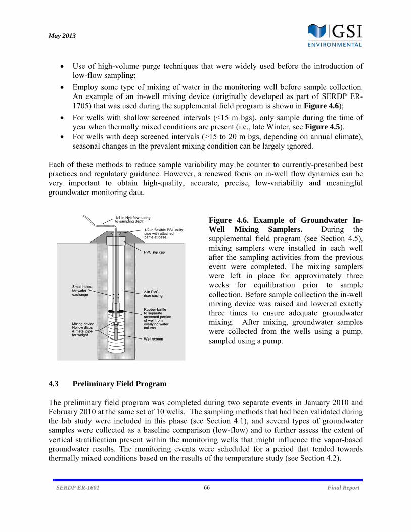
May 2013
SERDP ER-1601 66 Final Report
Use of high-volume purge techniques that were widely used before the introduction of low-flow sampling;
Employ some type of mixing of water in the monitoring well before sample collection. An example of an in-well mixing device (originally developed as part of SERDP ER-1705) that was used during the supplemental field program is shown in Figure 4.6);
For wells with shallow screened intervals (<15 m bgs), only sample during the time of year when thermally mixed conditions are present (i.e., late Winter, see Figure 4.5).
For wells with deep screened intervals (>15 to 20 m bgs, depending on annual climate), seasonal changes in the prevalent mixing condition can be largely ignored.
Each of these methods to reduce sample variability may be counter to currently-prescribed best practices and regulatory guidance. However, a renewed focus on in-well flow dynamics can be very important to obtain high-quality, accurate, precise, low-variability and meaningful groundwater monitoring data.
Figure 4.6. Example of Groundwater In-Well Mixing Samplers. During the supplemental field program (see Section 4.5), mixing samplers were installed in each well after the sampling activities from the previous event were completed. The mixing samplers were left in place for approximately three weeks for equilibration prior to sample collection. Before sample collection the in-well mixing device was raised and lowered exactly three times to ensure adequate groundwater mixing. After mixing, groundwater samples were collected from the wells using a pump. sampled using a pump.
4.3 Preliminary Field Program The preliminary field program was completed during two separate events in January 2010 and February 2010 at the same set of 10 wells. The sampling methods that had been validated during the lab study were included in this phase (see Section 4.1), and several types of groundwater samples were collected as a baseline comparison (low-flow) and to further assess the extent of vertical stratification present within the monitoring wells that might influence the vapor-based groundwater results. The monitoring events were scheduled for a period that tended towards thermally mixed conditions based on the results of the temperature study (see Section 4.2).
May 2013
SERDP ER-1601 67 Final Report
4.3.1 Well Characteristics and Sampling Data Table A.1 in Appendix A summarizes pertinent characteristics for the wells included in the field program. Monitoring was completed at 3 wells installed in unconfined aquifers and 7 wells installed in confined aquifers. The total depth of these wells ranged from approximately 18 ft to 69 ft, with a depth to water of between 4.5 and 38 feet. The majority of wells (8 of 10) had screens that were 10 ft in length, with the remainder (2 of 10) containing 5-ft long screens. In 17 of the 19 instances when the depth to water was measured (encompassing both sampling events), the water level was higher than the top of the screen interval. During the field program, groundwater and vapor samples were collected from each monitoring well using a series of different methods and analyzed either in the field or following shipment to a commercial laboratory. Table 4.8 summarizes the total number of samples collected using each of these methods. A total of 198 sample analyses were performed as part of the field program, not including replicates. For the six primary methods (bolded in Table 4.8), the objective was to collect 20 individual samples per method. This goal was not achievable for a variety of reasons:
One well was inadvertently opened prior to the start of the first sampling event, disturbing equilibrium conditions. No samples were collected from this well.
One or more pieces of equipment were compromised (e.g., obstructed tubing, pump failure) in several wells during the first sampling event.
The water level rose above the depth where the tubing for collecting a vapor sample terminated. During the first sampling event, this prevented the collection of vapor interface samples at two locations. When this condition was encountered during the second sampling event, the tubing was raised slightly above the water level and a vapor sample was collected.
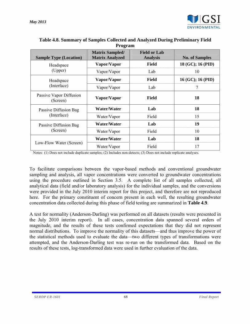
May 2013
SERDP ER-1601 68 Final Report
Table 4.8. Summary of Samples Collected and Analyzed During Preliminary Field Program
Sample Type (Location) Matrix Sampled/ Matrix Analyzed
Field or Lab Analysis No. of Samples
Headspace (Upper)
Vapor/Vapor Field 18 (GC); 16 (PID)
Vapor/Vapor Lab 10
Headspace (Interface)
Vapor/Vapor Field 16 (GC); 16 (PID)
Vapor/Vapor Lab 7
Passive Vapor Diffusion (Screen)
Vapor/Vapor Field 18
Passive Diffusion Bag (Interface)
Water/Water Lab 18
Water/Vapor Field 15
Passive Diffusion Bag (Screen)
Water/Water Lab 19
Water/Vapor Field 10
Low-Flow Water (Screen) Water/Water Lab 18
Water/Vapor Field 17 Notes: (1) Does not include duplicate samples; (2) Includes non-detects; (3) Does not include replicate analyses.
To facilitate comparisons between the vapor-based methods and conventional groundwater sampling and analysis, all vapor concentrations were converted to groundwater concentrations using the procedure outlined in Section 3.5. A complete list of all samples collected, all analytical data (field and/or laboratory analysis) for the individual samples, and the conversions were provided in the July 2010 interim report for this project, and therefore are not reproduced here. For the primary constituent of concern present in each well, the resulting groundwater concentration data collected during this phase of field testing are summarized in Table 4.9. A test for normality (Anderson-Darling) was performed on all datasets (results were presented in the July 2010 interim report). In all cases, concentration data spanned several orders of magnitude, and the results of these tests confirmed expectations that they did not represent normal distributions. To improve the normality of this datasets—and thus improve the power of the statistical methods used to evaluate the data—two different types of transformations were attempted, and the Anderson-Darling test was re-run on the transformed data. Based on the results of these tests, log-transformed data were used in further evaluation of the data.
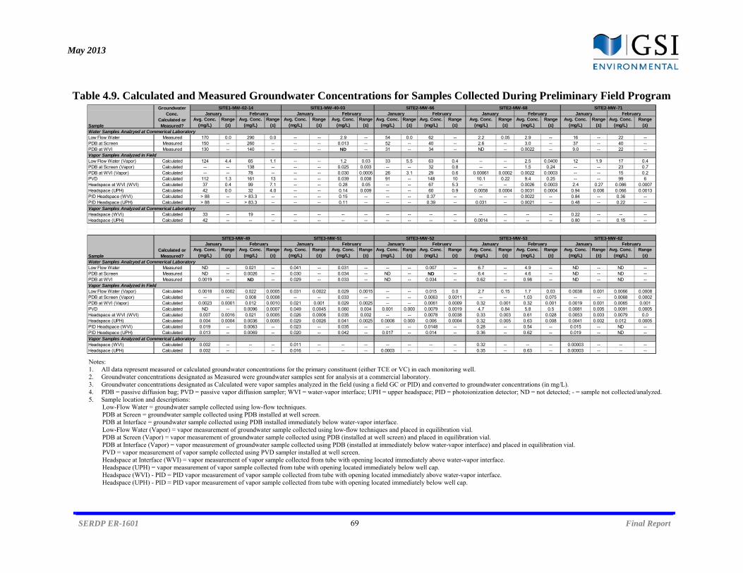
May 2013
SERDP ER-1601 69 Final Report
Table 4.9. Calculated and Measured Groundwater Concentrations for Samples Collected During Preliminary Field Program
Notes: 1. All data represent measured or calculated groundwater concentrations for the primary constituent (either TCE or VC) in each monitoring well. 2. Groundwater concentrations designated as Measured were groundwater samples sent for analysis at a commercial laboratory. 3. Groundwater concentrations designated as Calculated were vapor samples analyzed in the field (using a field GC or PID) and converted to groundwater concentrations (in mg/L). 4. PDB = passive diffusion bag; PVD = passive vapor diffusion sampler; WVI = water-vapor interface; UPH = upper headspace; PID = photoionization detector; ND = not detected; - = sample not collected/analyzed. 5. Sample location and descriptions:
Low-Flow Water = groundwater sample collected using low-flow techniques. PDB at Screen = groundwater sample collected using PDB installed at well screen. PDB at Interface = groundwater sample collected using PDB installed immediately below water-vapor interface. Low-Flow Water (Vapor) = vapor measurement of groundwater sample collected using low-flow techniques and placed in equilibration vial. PDB at Screen (Vapor) = vapor measurement of groundwater sample collected using PDB (installed at well screen) and placed in equilibration vial. PDB at Interface (Vapor) = vapor measurement of groundwater sample collected using PDB (installed at immediately below water-vapor interface) and placed in equilibration vial. PVD = vapor measurement of vapor sample collected using PVD sampler installed at well screen. Headspace at Interface (WVI) = vapor measurement of vapor sample collected from tube with opening located immediately above water-vapor interface. Headspace (UPH) = vapor measurement of vapor sample collected from tube with opening located immediately below well cap. Headspace (WVI) - PID = PID vapor measurement of vapor sample collected from tube with opening located immediately above water-vapor interface. Headspace (UPH) - PID = PID vapor measurement of vapor sample collected from tube with opening located immediately below well cap.
Avg. Conc. (mg/L)
Range(±)
Avg. Conc. (mg/L)
Range(±)
Avg. Conc. (mg/L)
Range(±)
Avg. Conc. (mg/L)
Range(±)
Avg. Conc. (mg/L)
Range(±)
Avg. Conc. (mg/L)
Range(±)
Avg. Conc. (mg/L)
Range(±)
Avg. Conc. (mg/L)
Range(±)
Avg. Conc. (mg/L)
Range(±)
Avg. Conc. (mg/L)
Range(±)
Water Samples Analzyed at Commerical LaboratoryLow Flow Water Measured 170 0.0 290 0.0 -- -- 2.9 -- 54 0.0 62 -- 2.2 0.05 2.9 -- 16 -- 22 --PDB at Screen Measured 150 -- 260 -- -- -- 0.013 -- 52 -- 40 -- 2.6 -- 3.0 -- 37 -- 40 --PDB at WVI Measured 130 -- 140 -- -- -- ND -- 31 -- 34 -- ND -- 0.0022 -- 9.0 -- 22 --Vapor Samples Analyzed in FieldLow Flow Water (Vapor) Calculated 124 4.4 65 1.1 -- -- 1.2 0.03 33 5.5 63 0.4 -- -- 2.5 0.0400 12 1.9 17 0.4PDB at Screen (Vapor) Calculated -- -- 138 -- -- -- 0.025 0.003 -- -- 32 0.8 -- -- 1.5 0.24 -- -- 23 0.7PDB at WVI (Vapor) Calculated -- -- 78 -- -- -- 0.030 0.0005 26 3.1 29 0.6 0.00061 0.0002 0.0022 0.0003 -- -- 15 0.2PVD Calculated 112 1.3 161 13 -- -- 0.039 0.008 91 -- 148 10 10.1 0.22 9.4 0.25 -- -- 99 6Headspace at WVI (WVI) Calculated 37 0.4 99 7.1 -- -- 0.28 0.05 -- -- 67 5.3 -- -- 0.0026 0.0003 2.4 0.27 0.086 0.0007Headspace (UPH) Calculated 42 0.0 32 4.0 -- -- 0.14 0.009 -- -- 60 0.9 0.0058 0.0004 0.0031 0.0004 0.94 0.006 0.066 0.0013PID Headspace (WVI) Calculated > 88 -- > 83.3 -- -- -- 0.15 -- -- -- 0.37 -- -- -- 0.0022 -- 0.84 -- 0.36 --PID Headspace (UPH) Calculated > 88 -- > 83.3 -- -- -- 0.11 -- -- -- 0.39 -- 0.031 -- 0.0021 -- 0.48 -- 0.22 --Vapor Samples Analyzed at Commerical LaboratoryHeadspace (WVI) Calculated 33 -- 19 -- -- -- -- -- -- -- -- -- -- -- -- -- 0.22 -- -- --Headspace (UPH) Calculated 42 -- -- -- -- -- -- -- -- -- -- -- 0.0014 -- -- -- 0.80 -- 0.15 --
Avg. Conc. (mg/L)
Range(±)
Avg. Conc. (mg/L)
Range(±)
Avg. Conc. (mg/L)
Range(±)
Avg. Conc. (mg/L)
Range(±)
Avg. Conc. (mg/L)
Range(±)
Avg. Conc. (mg/L)
Range(±)
Avg. Conc. (mg/L)
Range(±)
Avg. Conc. (mg/L)
Range(±)
Avg. Conc. (mg/L)
Range(±)
Avg. Conc. (mg/L)
Range(±)
Water Samples Analzyed at Commerical LaboratoryLow Flow Water Measured ND -- 0.021 -- 0.041 -- 0.031 -- -- -- 0.007 -- 6.7 -- 4.9 -- ND -- ND --PDB at Screen Measured ND -- 0.0026 -- 0.030 -- 0.034 -- ND -- ND -- 6.4 -- 4.6 -- ND -- ND --PDB at WVI Measured 0.0019 -- ND -- 0.029 -- 0.033 -- ND -- 0.034 -- 0.62 -- 0.98 -- ND -- ND --Vapor Samples Analyzed in FieldLow Flow Water (Vapor) Calculated 0.0018 0.0002 0.022 0.0005 0.031 0.0022 0.029 0.0015 -- -- 0.015 0.0 2.7 0.15 1.7 0.03 0.0038 0.001 0.0066 0.0008PDB at Screen (Vapor) Calculated -- -- 0.008 0.0008 -- -- 0.033 -- -- -- 0.0063 0.0011 -- -- 1.03 0.075 -- -- 0.0068 0.0002PDB at WVI (Vapor) Calculated 0.0023 0.0001 0.012 0.0010 0.021 0.001 0.029 0.0025 -- -- 0.0061 0.0009 0.32 0.001 0.32 0.001 0.0019 0.001 0.0065 0.001PVD Calculated ND -- 0.0096 0.0007 0.049 0.0045 0.060 0.004 0.001 0.000 0.0079 0.0019 4.7 0.84 5.8 0.5 0.0081 0.005 0.0091 0.0005Headspace at WVI (WVI) Calculated 0.007 0.0016 0.021 0.0005 0.026 0.0006 0.035 0.002 -- -- 0.0078 0.0038 0.33 0.003 0.61 0.028 0.0053 0.003 0.0079 0.0Headspace (UPH) Calculated 0.004 0.0004 0.0036 0.0005 0.029 0.0026 0.041 0.0025 0.0008 0.000 0.006 0.0004 0.32 0.005 0.63 0.008 0.0041 0.002 0.012 0.0005PID Headspace (WVI) Calculated 0.019 -- 0.0063 -- 0.023 -- 0.035 -- -- -- 0.0148 -- 0.28 -- 0.54 -- 0.015 -- ND --PID Headspace (UPH) Calculated 0.013 -- 0.0069 -- 0.020 -- 0.042 -- 0.017 -- 0.014 -- 0.36 -- 0.62 -- 0.019 -- ND --Vapor Samples Analyzed at Commerical LaboratoryHeadspace (WVI) Calculated 0.002 -- -- -- 0.011 -- -- -- -- -- -- -- 0.32 -- -- -- 0.00003 -- -- --Headspace (UPH) Calculated 0.002 -- -- -- 0.016 -- -- -- 0.0003 -- -- -- 0.35 -- 0.63 -- 0.00003 -- -- --
February January FebruarySITE3-MW-51
January February January February January
Groundwater Conc.
Calculated or Measured?
Calculated or Measured?
January FebruarySITE1-MW-02-14
January FebruarySITE3-MW-49
SITE2-MW-68January
SITE1-MW-40-03February
SITE3-MW-62
JanuarySITE2-MW-71
January February January February
SITE3-MW-52
Sample
February
Sample
SITE2-MW-66
SITE3-MW-53

May 2013
SERDP ER-1601 70 Final Report
4.3.2 Comparison of Vapor-Phase Based Methods to Low-Flow and Passive Groundwater Sampling
Comparisons were performed between groundwater concentration data calculated using field measurements of equilibrium vapor samples and groundwater concentration data measured using lab analysis of i) low-flow groundwater samples; and ii) groundwater samples collected using passive diffusion bags. Results of these comparisons are presented for the following evaluations:
i) Linear regression, using the correlation coefficient (R2) as an indicator of variability and the slope as an indicator of bias. Note that in addition to being presented and discussed in the following section, all linear regression plots from this phase of field testing are included in Figure A.1 of Appendix A for easy comparison.
ii) Two-sample tests (parametric and non-parametric) to determine if there is a statistically-significant difference between the means of the low-flow groundwater data and the groundwater data calculated using the vapor-phase based methods.
iii) Relative percent difference (RPD) between individual data pairs (e.g., low-flow vs. vapor-phase based concentration).
Data for these comparisons are presented in the following sub-sections. 4.3.2.1 Passive Vapor Diffusion Samplers Passive vapor diffusion samplers were installed at the screened interval for the monitoring well, at approximately the same depth interval where low-flow groundwater samples were collected. All vapor measurements were completed using the field GC (Figure 4.7) because insufficient sample volume was available for PID analysis. Collectively, the PVD data correlate well with the low-flow data, with no bias and only moderate variability. Because two samples were collected from the same vertical location in each well, there was unlikely to be any influence from in-well factors such as stratification. Note that a portion of these PVD results were presented in Adamson et al. (2012) without performing the pressure corrections on the concentration data (see Figure 2.3 for more information on the necessity of pressure corrections for certain scenarios). The wells included in this phase of field testing had relatively thin water columns above the samplers (median = 7 ft, maximum = 18 ft). This means that the hydrostatic pressure exerted only a marginal influence on the estimated groundwater concentration values. Passive diffusion bags installed at the well screen were also used to collect groundwater samples that were sent for off-site lab analysis, and a similar comparison can be made to measured concentrations from low-flow groundwater samples (Figure 4.8).
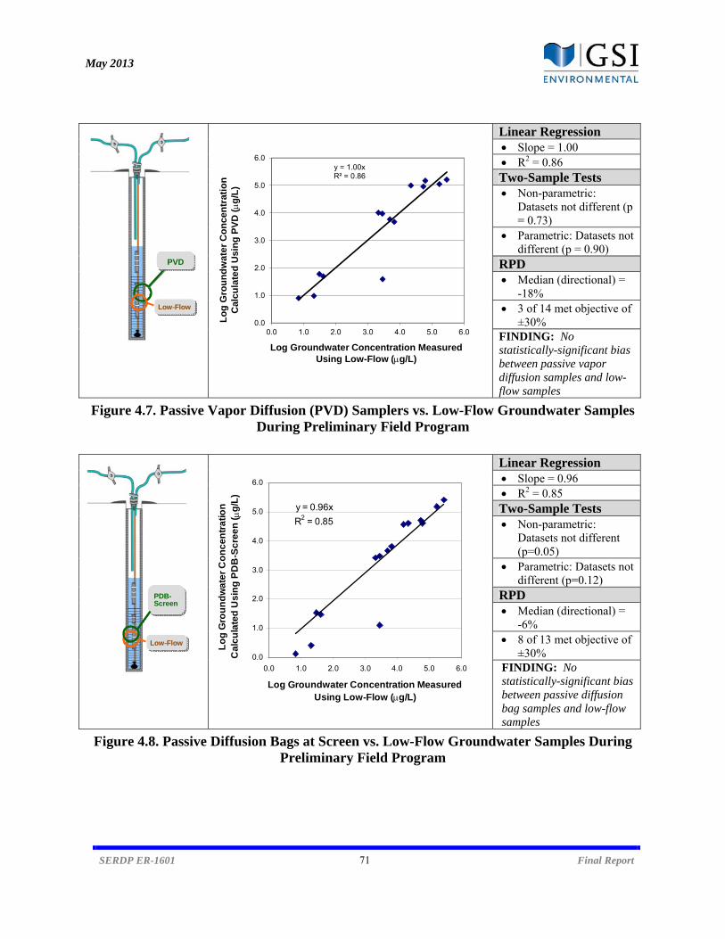
May 2013
SERDP ER-1601 71 Final Report
Linear Regression Slope = 1.00 R2 = 0.86 Two-Sample Tests Non-parametric:
Datasets not different (p = 0.73)
Parametric: Datasets not different (p = 0.90)
RPD Median (directional) =
-18% 3 of 14 met objective of
±30% FINDING: No statistically-significant bias between passive vapor diffusion samples and low-flow samples
Figure 4.7. Passive Vapor Diffusion (PVD) Samplers vs. Low-Flow Groundwater Samples During Preliminary Field Program
Linear Regression Slope = 0.96 R2 = 0.85 Two-Sample Tests Non-parametric:
Datasets not different (p=0.05)
Parametric: Datasets not different (p=0.12)
RPD Median (directional) =
-6% 8 of 13 met objective of
±30% FINDING: No statistically-significant bias between passive diffusion bag samples and low-flow samples
Figure 4.8. Passive Diffusion Bags at Screen vs. Low-Flow Groundwater Samples During Preliminary Field Program
y = 1.00xR² = 0.86
0.0
1.0
2.0
3.0
4.0
5.0
6.0
0.0 1.0 2.0 3.0 4.0 5.0 6.0
Lo
g G
rou
nd
wat
er C
on
cen
trat
ion
C
alc
ula
ted
Usi
ng
PV
D (g
/L)
Log Groundwater Concentration Measured Using Low-Flow (g/L)
y = 0.96x
R2 = 0.85
0.0
1.0
2.0
3.0
4.0
5.0
6.0
0.0 1.0 2.0 3.0 4.0 5.0 6.0
Log Groundwater Concentration Measured Using Low-Flow (g/L)
Lo
g G
rou
nd
wa
ter
Co
nc
en
tra
tio
n
Ca
lcu
late
d U
sin
g P
DB
-Sc
ree
n (g
/L)
PVD
Low-Flow
Low-Flow
PDB-Screen
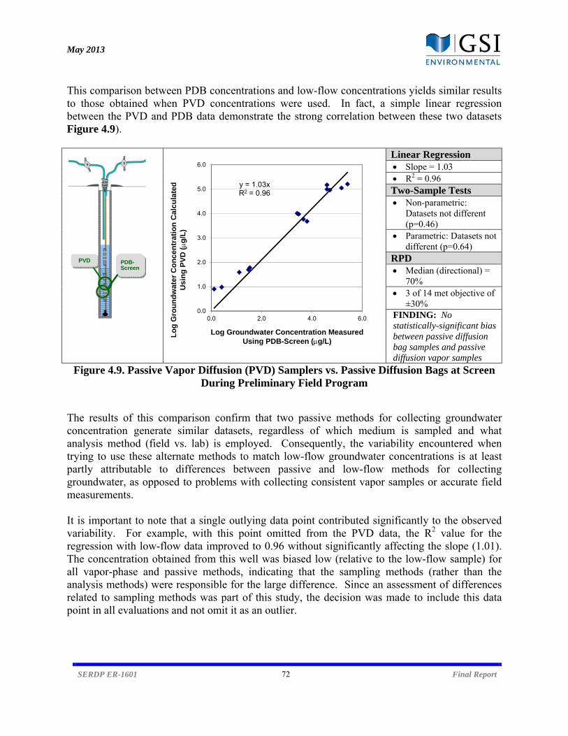
May 2013
SERDP ER-1601 72 Final Report
This comparison between PDB concentrations and low-flow concentrations yields similar results to those obtained when PVD concentrations were used. In fact, a simple linear regression between the PVD and PDB data demonstrate the strong correlation between these two datasets Figure 4.9).
Linear Regression Slope = 1.03 R2 = 0.96 Two-Sample Tests Non-parametric:
Datasets not different (p=0.46)
Parametric: Datasets not different (p=0.64)
RPD Median (directional) =
70% 3 of 14 met objective of
±30% FINDING: No statistically-significant bias between passive diffusion bag samples and passive diffusion vapor samples
Figure 4.9. Passive Vapor Diffusion (PVD) Samplers vs. Passive Diffusion Bags at Screen During Preliminary Field Program
The results of this comparison confirm that two passive methods for collecting groundwater concentration generate similar datasets, regardless of which medium is sampled and what analysis method (field vs. lab) is employed. Consequently, the variability encountered when trying to use these alternate methods to match low-flow groundwater concentrations is at least partly attributable to differences between passive and low-flow methods for collecting groundwater, as opposed to problems with collecting consistent vapor samples or accurate field measurements. It is important to note that a single outlying data point contributed significantly to the observed variability. For example, with this point omitted from the PVD data, the R2 value for the regression with low-flow data improved to 0.96 without significantly affecting the slope (1.01). The concentration obtained from this well was biased low (relative to the low-flow sample) for all vapor-phase and passive methods, indicating that the sampling methods (rather than the analysis methods) were responsible for the large difference. Since an assessment of differences related to sampling methods was part of this study, the decision was made to include this data point in all evaluations and not omit it as an outlier.
y = 1.03xR2 = 0.96
0.0
1.0
2.0
3.0
4.0
5.0
6.0
0.0 2.0 4.0 6.0
Lo
g G
rou
nd
wat
er C
on
cen
trat
ion
Cal
cu
late
d
Us
ing
PV
D (g
/L)
Log Groundwater Concentration Measured Using PDB-Screen (g/L)
PDB-Screen
PVD
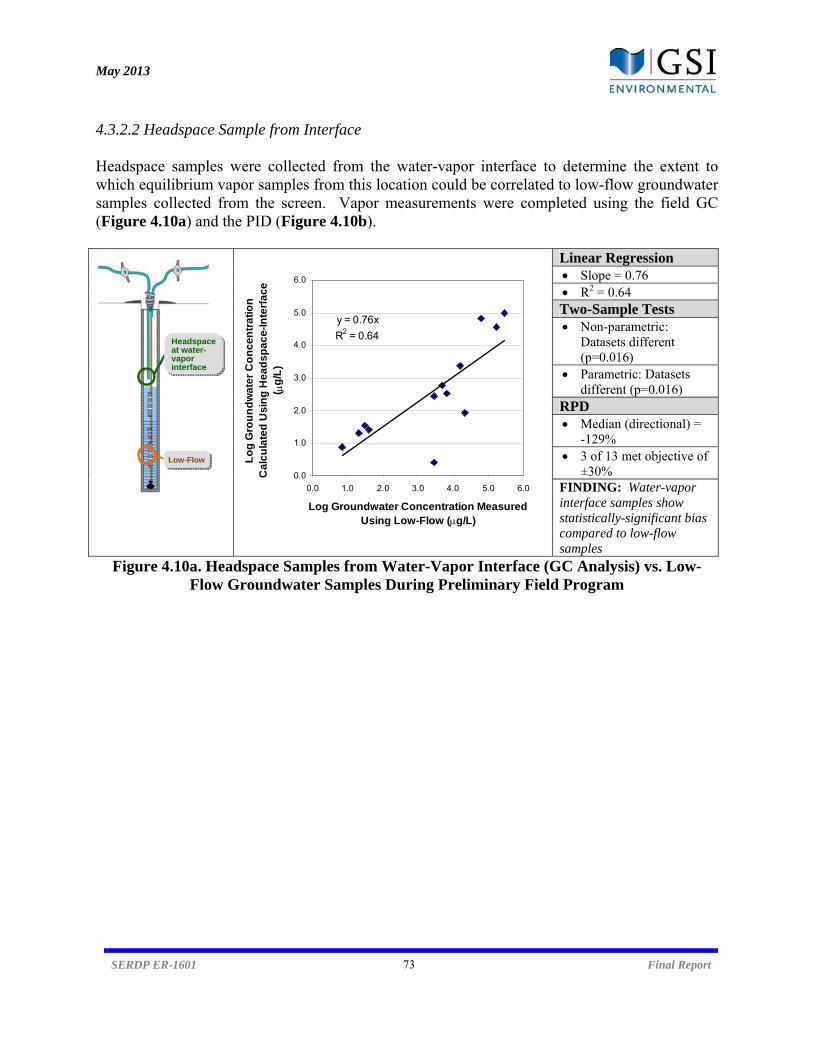
May 2013
SERDP ER-1601 73 Final Report
4.3.2.2 Headspace Sample from Interface Headspace samples were collected from the water-vapor interface to determine the extent to which equilibrium vapor samples from this location could be correlated to low-flow groundwater samples collected from the screen. Vapor measurements were completed using the field GC (Figure 4.10a) and the PID (Figure 4.10b).
Linear Regression Slope = 0.76 R2 = 0.64 Two-Sample Tests Non-parametric:
Datasets different (p=0.016)
Parametric: Datasets different (p=0.016)
RPD Median (directional) =
-129% 3 of 13 met objective of
±30% FINDING: Water-vapor interface samples show statistically-significant bias compared to low-flow samples
Figure 4.10a. Headspace Samples from Water-Vapor Interface (GC Analysis) vs. Low-Flow Groundwater Samples During Preliminary Field Program
y = 0.76x
R2 = 0.64
0.0
1.0
2.0
3.0
4.0
5.0
6.0
0.0 1.0 2.0 3.0 4.0 5.0 6.0
Log Groundwater Concentration Measured Using Low-Flow (g/L)
Lo
g G
rou
nd
wat
er
Co
nce
ntr
ati
on
C
alc
ula
ted
Usi
ng
Hea
dsp
ac
e-In
terf
ace
(
g/L
)
Headspace at water-vapor interface
Low-Flow
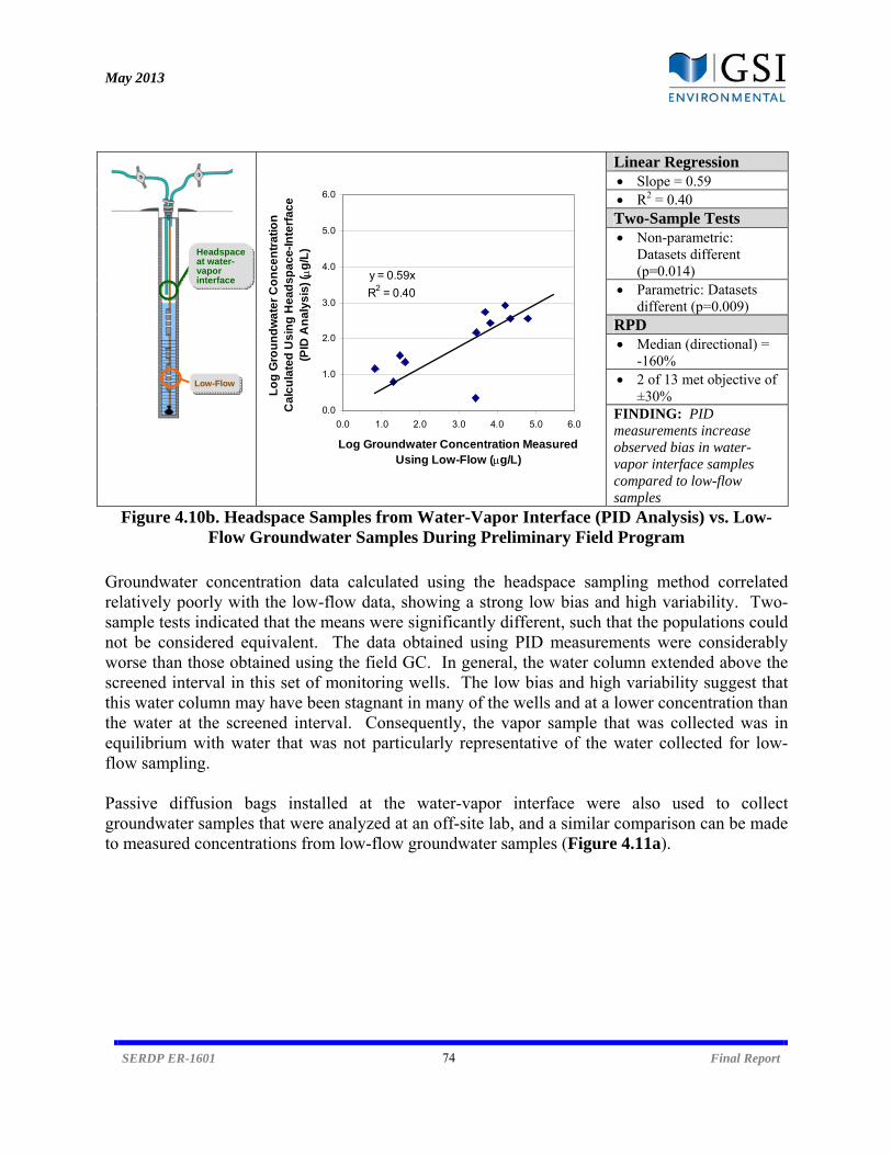
May 2013
SERDP ER-1601 74 Final Report
Linear Regression Slope = 0.59 R2 = 0.40 Two-Sample Tests Non-parametric:
Datasets different (p=0.014)
Parametric: Datasets different (p=0.009)
RPD Median (directional) =
-160% 2 of 13 met objective of
±30% FINDING: PID measurements increase observed bias in water-vapor interface samples compared to low-flow samples
Figure 4.10b. Headspace Samples from Water-Vapor Interface (PID Analysis) vs. Low-Flow Groundwater Samples During Preliminary Field Program
Groundwater concentration data calculated using the headspace sampling method correlated relatively poorly with the low-flow data, showing a strong low bias and high variability. Two-sample tests indicated that the means were significantly different, such that the populations could not be considered equivalent. The data obtained using PID measurements were considerably worse than those obtained using the field GC. In general, the water column extended above the screened interval in this set of monitoring wells. The low bias and high variability suggest that this water column may have been stagnant in many of the wells and at a lower concentration than the water at the screened interval. Consequently, the vapor sample that was collected was in equilibrium with water that was not particularly representative of the water collected for low-flow sampling. Passive diffusion bags installed at the water-vapor interface were also used to collect groundwater samples that were analyzed at an off-site lab, and a similar comparison can be made to measured concentrations from low-flow groundwater samples (Figure 4.11a).
y = 0.59x
R2 = 0.40
0.0
1.0
2.0
3.0
4.0
5.0
6.0
0.0 1.0 2.0 3.0 4.0 5.0 6.0
Log Groundwater Concentration Measured Using Low-Flow (g/L)
Lo
g G
rou
nd
wa
ter
Co
nce
ntr
atio
n
Ca
lcu
late
d U
sin
g H
ead
spa
ce-
Inte
rfac
e
(PID
An
aly
sis
) (
g/L
)
Low-Flow
Headspace at water-vapor interface

May 2013
SERDP ER-1601 75 Final Report
Linear Regression Slope = 0.82 R2 = 0.60 Two-Sample Tests Non-parametric:
Datasets different (p=0.019)
Parametric: Datasets different (p=0.049)
RPD Median (directional) =
-73% 3 of 12 met objective of
±30% FINDING: Statistically-significant difference between passive diffusion bag samples collected at water-vapor interface and low-flow samples
Figure 4.11a. Passive Diffusion Bags at Water-Vapor Interface vs. Low-Flow Groundwater Samples During Preliminary Field Program
This comparison between PDB concentrations and low-flow concentrations yielded slightly better results than those obtained when headspace-based concentrations were used, but the correlation remained relatively poor. Considerable variability was apparent in both datasets, suggesting an apparent difficulty in obtaining a consistent sample from the water-vapor interface in a monitoring well. This is further illustrated by a direct comparison between concentrations from the PDB at the interface and concentrations calculated using the headspace sampled at the interface (Figure 4.11b). There was less bias between the two datasets (slope = 0.87), as would be expected from their similar sampling location near the interface. The two-sample tests indicated that there was no statistically significant difference between the datasets. However, the R2 value remained low (0.60), confirming that sampling near the interface introduced a considerable amount of variability into the monitoring data.
y = 0.82x
R2 = 0.60
0.0
1.0
2.0
3.0
4.0
5.0
6.0
0.0 1.0 2.0 3.0 4.0 5.0 6.0
Log Groundwater Concentration Measured Using Low-Flow (g/L)
Lo
g G
rou
nd
wa
ter
Co
nc
en
tra
tion
C
alc
ula
ted
Us
ing
PD
B-I
nte
rfa
ce
(g
/L)
Low-Flow
PDB-Interface

May 2013
SERDP ER-1601 76 Final Report
Linear Regression Slope = 0.87 R2 = 0.60 Two-Sample Tests Non-parametric:
Datasets not different (p=0.62)
Parametric: Datasets not different (p=0.93)
RPD Median (directional) =
-40% 3 of 12 met objective of
±30% FINDING: No statistically-significant difference between passive diffusion bag and headspace samples collected at water-vapor interface, but sample location introduces variability
Figure 4.11b. Headspace Samples from Water-Vapor Interface (GC Analysis) vs. Passive Diffusion Bags at Water-Vapor Interface During Preliminary Field Program
4.3.2.3 Upper Headspace Sample Headspace samples were collected from the upper portion of the well to determine the extent to which equilibrium vapor samples in this location could be correlated to low-flow groundwater samples collected from the screen. Vapor measurements were completed using the field GC (Figure 4.12a) and the PID (Figure 4.12b). As with the headspace-interface dataset, the groundwater concentration data calculated using the upper headspace sampling method correlated relatively poorly with the low-flow data. The vapor-phase measurements were consistently biased low with high variability, and two-sample tests indicated that the means were significantly different. The data obtained using PID measurements again were again worse than those obtained using the field GC.
y = 0.87x
R2 = 0.60
0.0
1.0
2.0
3.0
4.0
5.0
6.0
0.0 1.0 2.0 3.0 4.0 5.0 6.0
Log Groundwater Concentration Measured Using PDB-Interface (g/L)
GW
Co
nc
en
tra
tio
n C
alc
ula
ted
Us
ing
H
ea
ds
pa
ce
-In
terf
ac
e (
g/L
)Headspace at water-vapor interface
PDB-Interface
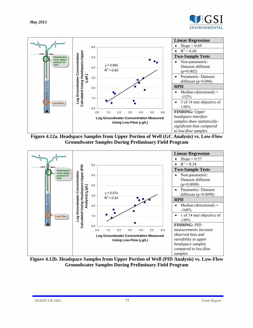
May 2013
SERDP ER-1601 77 Final Report
Linear Regression Slope = 0.69 R2 = 0.60 Two-Sample Tests Non-parametric:
Datasets different (p=0.002)
Parametric: Datasets different (p=0.006)
RPD Median (directional) =
-152% 3 of 14 met objective of
±30% FINDING: Upper headspace interface samples show statistically-significant bias compared to low-flow samples
Figure 4.12a. Headspace Samples from Upper Portion of Well (GC Analysis) vs. Low-Flow Groundwater Samples During Preliminary Field Program
Linear Regression Slope = 0.57 R2 = 0.34 Two-Sample Tests Non-parametric:
Datasets different (p=0.0098)
Parametric: Datasets different (p=0.0098)
RPD Median (directional) =
-168% 1 of 14 met objective of
±30% FINDING: PID measurements increase observed bias and variability in upper headspace samples compared to low-flow samples
Figure 4.12b. Headspace Samples from Upper Portion of Well (PID Analysis) vs. Low-Flow Groundwater Samples During Preliminary Field Program
y = 0.69x
R2 = 0.60
0.0
1.0
2.0
3.0
4.0
5.0
6.0
0.0 1.0 2.0 3.0 4.0 5.0 6.0
Log Groundwater Concentration Measured Using Low-Flow (g/L)
Lo
g G
rou
nd
wa
ter
Co
nc
entr
atio
n
Ca
lcu
late
d U
sin
g H
ea
dsp
ac
e-U
pp
er
( g
/L)
y = 0.57x
R2 = 0.34
0.0
1.0
2.0
3.0
4.0
5.0
6.0
0.0 1.0 2.0 3.0 4.0 5.0 6.0
Log Groundwater Concentration Measured Using Low-Flow (g/L)
Lo
g G
rou
nd
wa
ter
Co
nc
en
tra
tio
n
Ca
lcu
late
d U
sin
g H
ea
ds
pa
ce
-Up
pe
r (P
ID
An
aly
sis
) (
g/L
)
Low-Flow
Low-Flow
Headspace from upper portion of well
Headspace from upper portion of well
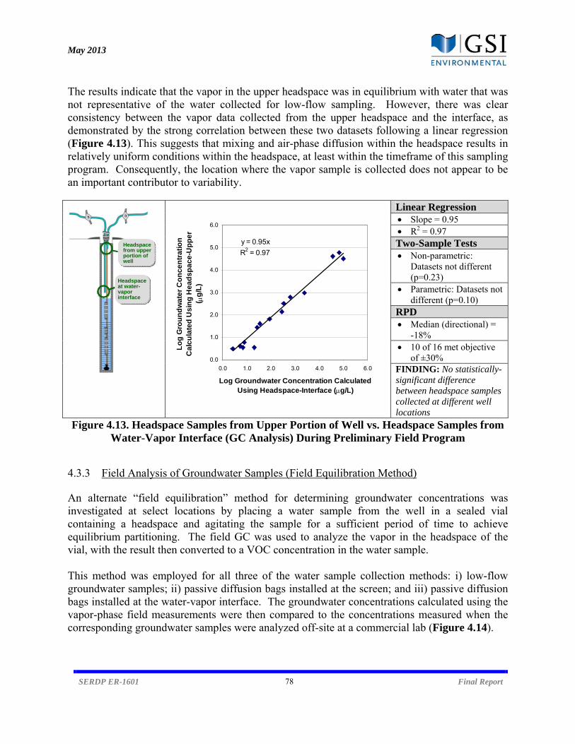
May 2013
SERDP ER-1601 78 Final Report
The results indicate that the vapor in the upper headspace was in equilibrium with water that was not representative of the water collected for low-flow sampling. However, there was clear consistency between the vapor data collected from the upper headspace and the interface, as demonstrated by the strong correlation between these two datasets following a linear regression (Figure 4.13). This suggests that mixing and air-phase diffusion within the headspace results in relatively uniform conditions within the headspace, at least within the timeframe of this sampling program. Consequently, the location where the vapor sample is collected does not appear to be an important contributor to variability.
Linear Regression Slope = 0.95 R2 = 0.97 Two-Sample Tests Non-parametric:
Datasets not different (p=0.23)
Parametric: Datasets not different (p=0.10)
RPD Median (directional) =
-18% 10 of 16 met objective
of ±30% FINDING: No statistically-significant difference between headspace samples collected at different well locations
Figure 4.13. Headspace Samples from Upper Portion of Well vs. Headspace Samples from Water-Vapor Interface (GC Analysis) During Preliminary Field Program
4.3.3 Field Analysis of Groundwater Samples (Field Equilibration Method) An alternate “field equilibration” method for determining groundwater concentrations was investigated at select locations by placing a water sample from the well in a sealed vial containing a headspace and agitating the sample for a sufficient period of time to achieve equilibrium partitioning. The field GC was used to analyze the vapor in the headspace of the vial, with the result then converted to a VOC concentration in the water sample. This method was employed for all three of the water sample collection methods: i) low-flow groundwater samples; ii) passive diffusion bags installed at the screen; and iii) passive diffusion bags installed at the water-vapor interface. The groundwater concentrations calculated using the vapor-phase field measurements were then compared to the concentrations measured when the corresponding groundwater samples were analyzed off-site at a commercial lab (Figure 4.14).
y = 0.95x
R2 = 0.97
0.0
1.0
2.0
3.0
4.0
5.0
6.0
0.0 1.0 2.0 3.0 4.0 5.0 6.0
Log Groundwater Concentration Calculated Using Headspace-Interface (g/L)
Lo
g G
rou
nd
wa
ter
Co
nc
en
tra
tio
n
Ca
lcu
late
d U
sin
g H
ea
ds
pa
ce
-Up
pe
r (
g/L
)
Headspace from upper portion of well
Headspace at water-vapor interface
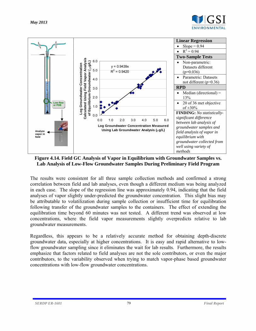
May 2013
SERDP ER-1601 79 Final Report
Linear Regression Slope = 0.94 R2 = 0.94 Two-Sample Tests Non-parametric:
Datasets different (p=0.036)
Parametric: Datasets not different (p=0.36)
RPD Median (directional) =
13% 20 of 36 met objective
of ±30% FINDING: No statistically-significant difference between lab analysis of groundwater samples and field analysis of vapor in equilibrium with groundwater collected from well using variety of methods
Figure 4.14. Field GC Analysis of Vapor in Equilibrium with Groundwater Samples vs. Lab Analysis of Low-Flow Groundwater Samples During Preliminary Field Program
The results were consistent for all three sample collection methods and confirmed a strong correlation between field and lab analyses, even though a different medium was being analyzed in each case. The slope of the regression line was approximately 0.94, indicating that the field analyses of vapor slightly under-predicted the groundwater concentration. This slight bias may be attributable to volatilization during sample collection or insufficient time for equilibration following transfer of the groundwater samples to the containers. The effect of extending the equilibration time beyond 60 minutes was not tested. A different trend was observed at low concentrations, where the field vapor measurements slightly overpredicts relative to lab groundwater measurements. Regardless, this appears to be a relatively accurate method for obtaining depth-discrete groundwater data, especially at higher concentrations. It is easy and rapid alternative to low-flow groundwater sampling since it eliminates the wait for lab results. Furthermore, the results emphasize that factors related to field analyses are not the sole contributors, or even the major contributors, to the variability observed when trying to match vapor-phase based groundwater concentrations with low-flow groundwater concentrations.
y = 0.9439x
R2 = 0.9420
0.0
1.0
2.0
3.0
4.0
5.0
6.0
0.0 1.0 2.0 3.0 4.0 5.0 6.0
Log Groundwater Concentration Measured Using Lab Groundwater Analysis (g/L)
Lo
g G
rou
nd
wa
ter
Co
nc
en
tra
tio
n
Ca
lcu
late
d U
sin
g F
ield
Va
po
r A
na
lys
is
of
Eq
uil
ibri
um
Gro
un
dw
ate
r (g
/L)
Low-flow or PDB
Analyze vapor in field
May 2013
SERDP ER-1601 80 Final Report
4.3.4 Evaluation of Precision and Accuracy for Field and Lab Analyses In addition to the results presented in Section 4.3.3, several other methods were employed to investigate the precision and accuracy of the various sampling and analyses methods. 4.3.4.1 Laboratory and Field Analyses of Replicate Samples Both groundwater and vapor duplicate samples were collected for analysis at (separate) commercial laboratories. A small set of duplicate vapor samples were also collected for field analysis. For each set of duplicates, the relative standard deviation (RSD) was calculated as a metric for assessing precision (Table 4.10).
Table 4.10. Precision of Laboratory vs. Field Analyses of Duplicate Samples
Analysis Type No. of Duplicate
Sample Sets RSD (%)
Range Mean Groundwater (Lab) 5(1) 0.0 – 12.4 % 3.7 %
Vapor (Lab) 2 2.5 – 6.4 % 4.4 % Vapor (Field) 2 0.16 – 0.5 % 0.3 %
Notes: (1) Does not include two additional duplicate sample sets where concentration was below lab reporting limit.
While the sample set was relatively small, the level of precision for field analyses of duplicates was equal to or better than that for lab analyses. Note that the RSD values in Table 4.10 reflect variability associated with the sampling steps as well as the analysis steps. 4.3.4.2 Replicate Field Analyses of Vapor Samples Replicate analyses of all vapor samples were completed in the field to provide a more focused assessment of the precision of the equipment under field conditions. The data in Table 4.11 represent RSD values calculated from duplicate or triplicate analyses using the field GC (note that insufficient sample volume was available to complete replicate analyses with the PID).
Table 4.11. Precision of Replicate Field Analyses of All Samples
Analysis Type No. of Replicate
Analysis Sets RSD (%)
Range Mean Median Vapor (Field) 96 0.4 – 112 % 11.9 % 7.9 %
Because of the large sample size, the RSD values for this set of measurements are likely to be a more representative indicator of the precision of the field instruments. Greater than 90% of the RSD values met the general performance objective of < 30% RSD. There was no evidence that any particular sample type (e.g., upper headspace sample, PVD, etc.) contributed to higher RSD values following replicate analyses. The median RSD value for the instrument under field conditions (7.9%) was only slightly higher than the median RSD value for the same instrument during the laboratory validation study (2.0%).
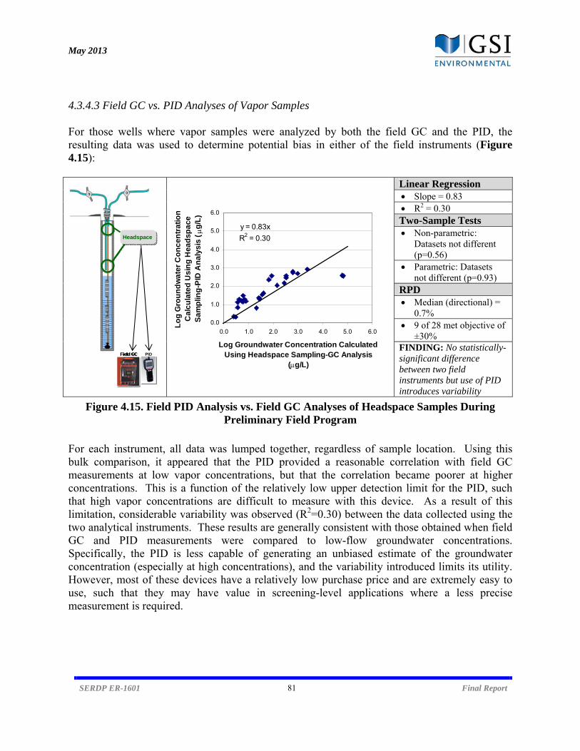
May 2013
SERDP ER-1601 81 Final Report
4.3.4.3 Field GC vs. PID Analyses of Vapor Samples For those wells where vapor samples were analyzed by both the field GC and the PID, the resulting data was used to determine potential bias in either of the field instruments (Figure 4.15):
Linear Regression Slope = 0.83 R2 = 0.30 Two-Sample Tests Non-parametric:
Datasets not different (p=0.56)
Parametric: Datasets not different (p=0.93)
RPD Median (directional) =
0.7% 9 of 28 met objective of
±30% FINDING: No statistically-significant difference between two field instruments but use of PID introduces variability
Figure 4.15. Field PID Analysis vs. Field GC Analyses of Headspace Samples During Preliminary Field Program
For each instrument, all data was lumped together, regardless of sample location. Using this bulk comparison, it appeared that the PID provided a reasonable correlation with field GC measurements at low vapor concentrations, but that the correlation became poorer at higher concentrations. This is a function of the relatively low upper detection limit for the PID, such that high vapor concentrations are difficult to measure with this device. As a result of this limitation, considerable variability was observed (R2=0.30) between the data collected using the two analytical instruments. These results are generally consistent with those obtained when field GC and PID measurements were compared to low-flow groundwater concentrations. Specifically, the PID is less capable of generating an unbiased estimate of the groundwater concentration (especially at high concentrations), and the variability introduced limits its utility. However, most of these devices have a relatively low purchase price and are extremely easy to use, such that they may have value in screening-level applications where a less precise measurement is required.
y = 0.83x
R2 = 0.30
0.0
1.0
2.0
3.0
4.0
5.0
6.0
0.0 1.0 2.0 3.0 4.0 5.0 6.0
Log Groundwater Concentration Calculated Using Headspace Sampling-GC Analysis
(g/L)
Lo
g G
rou
nd
wa
ter
Co
nc
entr
atio
n
Ca
lcu
late
d U
sin
g H
ead
spa
ce
Sa
mp
ling
-PID
An
aly
sis
(
g/L
)
PID
Headspace
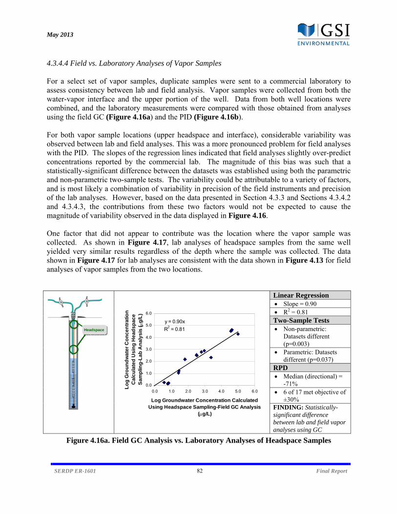
May 2013
SERDP ER-1601 82 Final Report
4.3.4.4 Field vs. Laboratory Analyses of Vapor Samples For a select set of vapor samples, duplicate samples were sent to a commercial laboratory to assess consistency between lab and field analysis. Vapor samples were collected from both the water-vapor interface and the upper portion of the well. Data from both well locations were combined, and the laboratory measurements were compared with those obtained from analyses using the field GC (Figure 4.16a) and the PID (Figure 4.16b). For both vapor sample locations (upper headspace and interface), considerable variability was observed between lab and field analyses. This was a more pronounced problem for field analyses with the PID. The slopes of the regression lines indicated that field analyses slightly over-predict concentrations reported by the commercial lab. The magnitude of this bias was such that a statistically-significant difference between the datasets was established using both the parametric and non-parametric two-sample tests. The variability could be attributable to a variety of factors, and is most likely a combination of variability in precision of the field instruments and precision of the lab analyses. However, based on the data presented in Section 4.3.3 and Sections 4.3.4.2 and 4.3.4.3, the contributions from these two factors would not be expected to cause the magnitude of variability observed in the data displayed in Figure 4.16. One factor that did not appear to contribute was the location where the vapor sample was collected. As shown in Figure 4.17, lab analyses of headspace samples from the same well yielded very similar results regardless of the depth where the sample was collected. The data shown in Figure 4.17 for lab analyses are consistent with the data shown in Figure 4.13 for field analyses of vapor samples from the two locations.
Linear Regression Slope = 0.90 R2 = 0.81 Two-Sample Tests Non-parametric:
Datasets different (p=0.003)
Parametric: Datasets different (p=0.037)
RPD Median (directional) =
-71% 6 of 17 met objective of
±30% FINDING: Statistically-significant difference between lab and field vapor analyses using GC
Figure 4.16a. Field GC Analysis vs. Laboratory Analyses of Headspace Samples
y = 0.90x
R2 = 0.81
0.0
1.0
2.0
3.0
4.0
5.0
6.0
0.0 1.0 2.0 3.0 4.0 5.0 6.0
Log Groundwater Concentration Calculated Using Headspace Sampling-Field GC Analysis
(g/L)
Lo
g G
rou
nd
wa
ter
Co
nc
en
tra
tio
n
Ca
lcu
late
d U
sin
g H
ea
ds
pa
ce
S
am
plin
g-L
ab
An
aly
sis
( g
/L)
Headspace
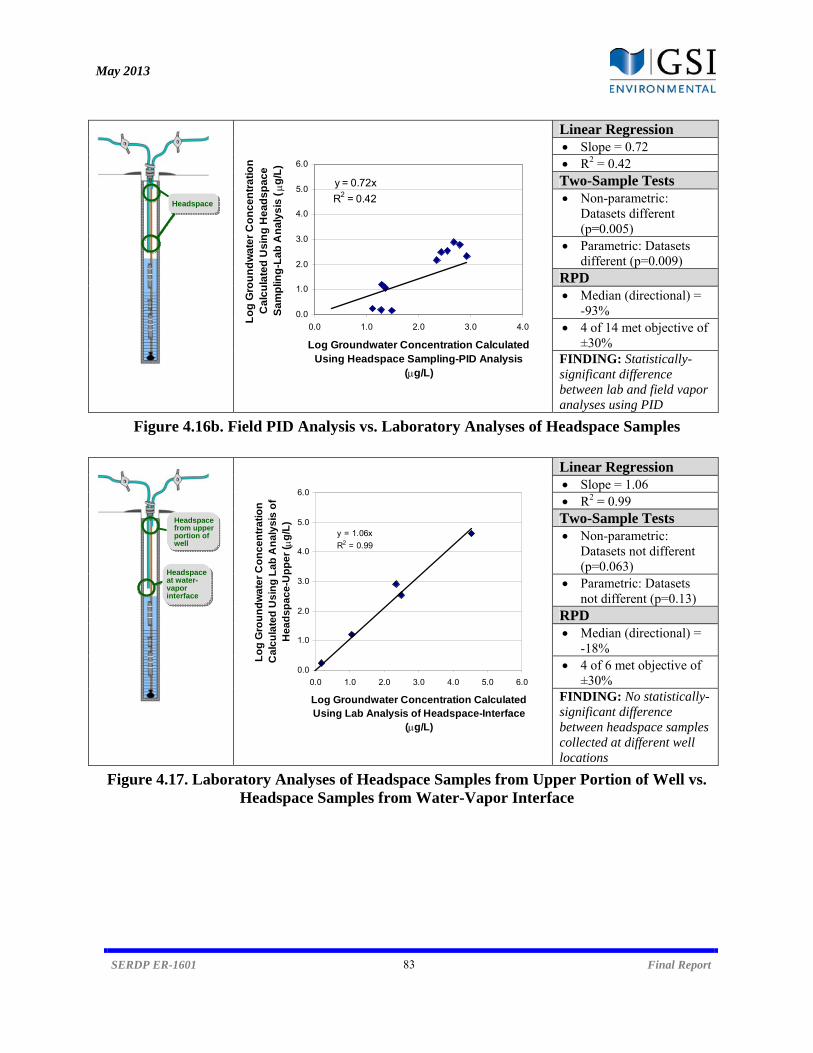
May 2013
SERDP ER-1601 83 Final Report
Linear Regression Slope = 0.72 R2 = 0.42 Two-Sample Tests Non-parametric:
Datasets different (p=0.005)
Parametric: Datasets different (p=0.009)
RPD Median (directional) =
-93% 4 of 14 met objective of
±30% FINDING: Statistically-significant difference between lab and field vapor analyses using PID
Figure 4.16b. Field PID Analysis vs. Laboratory Analyses of Headspace Samples
Linear Regression Slope = 1.06 R2 = 0.99 Two-Sample Tests Non-parametric:
Datasets not different (p=0.063)
Parametric: Datasets not different (p=0.13)
RPD Median (directional) =
-18% 4 of 6 met objective of
±30% FINDING: No statistically-significant difference between headspace samples collected at different well locations
Figure 4.17. Laboratory Analyses of Headspace Samples from Upper Portion of Well vs. Headspace Samples from Water-Vapor Interface
y = 0.72x
R2 = 0.42
0.0
1.0
2.0
3.0
4.0
5.0
6.0
0.0 1.0 2.0 3.0 4.0
Log Groundwater Concentration Calculated Using Headspace Sampling-PID Analysis
(g/L)
Lo
g G
rou
nd
wa
ter
Co
nc
en
tra
tio
n
Ca
lcu
late
d U
sin
g H
ea
ds
pa
ce
S
am
plin
g-L
ab
An
aly
sis
(
g/L
)
y = 1.06x
R2 = 0.99
0.0
1.0
2.0
3.0
4.0
5.0
6.0
0.0 1.0 2.0 3.0 4.0 5.0 6.0
Log Groundwater Concentration Calculated Using Lab Analysis of Headspace-Interface
(g/L)
Lo
g G
rou
nd
wa
ter
Co
nc
en
tra
tio
n
Ca
lcu
late
d U
sin
g L
ab
An
aly
sis
of
He
ad
sp
ac
e-U
pp
er
( g
/L)Headspace
from upper portion of well
Headspace
Headspace at water-vapor interface
May 2013
SERDP ER-1601 84 Final Report
4.3.5 Summary of Factors Contributing to Bias and Variability The data from the field program was sufficient to investigate a number of factors that may have contributed to bias and variability between datasets. A summary is provided below:
Vertical Stratification: Concentrations within the monitoring well water column did not appear to be uniform with depth within the majority of locations included in this program, as evidenced by the differences between samples collected from the well screen and the water-vapor interface (e.g., Figure 4.11a). Multi-level sampling data collected from two of the wells during an earlier period (November 2009) as part of the temperature study indicates the extent of stratification that can occur in at least a subset of the wells (Figure 4.5). During the expanded field program, further evidence of stratification is shown by the lack of strong correlation between passive water samples at the screen vs. passive water samples at the interface (Figure 4.19). Collectively, these data indicate that in-well mixing may have been limited, even though the data was collected during winter months when thermal instability (i.e., colder, denser water at the surface) would be expected to promote mixing. A lack of in-well mixing limits the ability to collect a well headspace sample that is representative of low-flow groundwater concentration because the air column is in equilibrium with a water concentration that is different from that at the screen. However, it also emphasizes that groundwater concentration data should not necessarily be taken at face value and proper interpretation must consider the well-specific effects of vertical stratification.
Sample Location: Because of the influence of vertical stratification, the location where
samples were collected was very important in minimizing bias. This is particularly evident in samples within the water column. Within the well headspace, sample location was not as important a factor (Figure 4.13, Figure 4.17), presumably due to the ability of compounds to diffuse rapidly in the vapor-phase. For the purposes of correlating vapor samples with groundwater concentrations, the data indicate that samples should be collected from the same vertical location of the well to minimize bias.
Sample Collection Method: Vapor samples from the headspace introduced a
considerable amount of variability into the datasets, as evidenced by the low R2 values in Figure 4.10 and Figure 4.11. Passive vapor samples resulted in less variability and no significant bias relative to low-flow groundwater samples. An even higher correlation was observed between concentrations obtained from passive vapor and those from passive groundwater samples (Figure 4.9). These data suggest that passive vapor methods result in a more consistent sample than headspace sampling, but they also emphasize that passive methods (both vapor and groundwater) occasionally yield different results than low-flow methods. Passive methods are thought to be less reliable for low permeability aquifers (ITRC, 2004), but the reasons for differences between low-flow and passive samples are generally not well-understood. Unlike passive methods, the process of low-flow purging may induce mixing, indicating that low-flow samples more
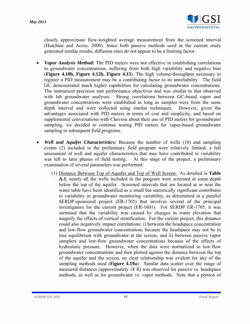
May 2013
SERDP ER-1601 85 Final Report
closely approximate flow-weighted average measurement from the screened interval (Hutchins and Acree, 2000). Since both passive methods used in the current study generated similar results, diffusion rates do not appear to be a limiting factor.
Vapor Analysis Method: The PID meters were not effective in establishing correlations
to groundwater concentrations, suffering from both high variability and negative bias (Figure 4.10b, Figure 4.12b, Figure 4.15). The high volume-throughput necessary to register a PID measurement may be a contributing factor to its unreliability. The field GC demonstrated much higher capabilities for calculating groundwater concentrations. The instrument precision met performance objectives and was similar to that observed with lab groundwater analyses. Strong correlations between GC-based vapor and groundwater concentrations were established as long as samples were from the same depth interval and were collected using similar techniques. However, given the advantages associated with PID meters in terms of cost and simplicity, and based on supplemental conversations with Chevron about their use of PID meters for groundwater sampling, we decided to continue testing PID meters for vapor-based groundwater sampling in subsequent field programs.
Well and Aquifer Characteristics: Because the number of wells (10) and sampling
events (2) included in the preliminary field program were relatively limited, a full assessment of well and aquifer characteristics that may have contributed to variability was left to later phases of field testing. At this stage of the project, a preliminary examination of several parameters was performed:
(1) Distance Between Top of Aquifer and Top of Well Screen: As detailed in Table A.1, nearly all the wells included in the program were screened at some depth below the top of the aquifer. Screened intervals that are located at or near the water table have been identified as a small but statistically significant contributor to variability in groundwater monitoring variability, as determined in a parallel SERDP-sponsored project (ER-1705) that involves several of the principal investigators for the current project (ER-1601). For SERDP ER-1705, it was surmised that the variability was caused by changes in water elevation that magnify the effects of vertical stratification. For the current project, this distance could also negatively impact correlations: i) between the headspace concentration and low-flow groundwater concentrations because the headspace may not be in true equilibrium with groundwater at the screen; and ii) between passive vapor samplers and low-flow groundwater concentrations because of the effects of hydrostatic pressure. However, when the data were normalized to low-flow groundwater concentrations and then plotted against the distance between the top of the aquifer and the screen, no clear relationship was evident for any of the sampling methods used (Figure 4.19a). Similar data scatter over the range of measured distances (approximately 18 ft) was observed for passive vs. headspace methods, as well as for groundwater vs. vapor methods. Note that a portion of

May 2013
SERDP ER-1601 86 Final Report
these results were presented in Adamson et al. (2012) without performing the pressure corrections on the concentration data obtained with the short PVD samplers. The wells included in this phase of field testing had relatively thin water columns above the samplers (again, 18 ft or less), such that the hydrostatic pressure did not exert a major influence on the estimated groundwater concentration values.
(2) Depth to Top of Aquifer: Shallow wells tend to more influenced by temperature gradients from the surface, and as a consequence, would be more prone to experience in-well mixing due to temperature changes. Based on data from the current study, shallow wells may be weakly correlated to over-predictions of the low-flow groundwater concentration (Figure 4.19b). This pattern appeared to be more prevalent for samples collected with passive methods.
(3) Length of Well Screen: The length of the well screen is likely to have a significant impact on concentrations in wells where vertical stratification occurs. Shorter screens are more appropriate for assessing depth-specific concentrations, and (all other factors being equal) would be expected to result in stronger correlations between vapor and groundwater concentrations. In the current field program, 8 of the 10 wells had 10-ft long screens, while only 2 of 10 had 5-ft long screens. Of the wells with 5-ft long screens, only one had a low-flow groundwater concentration greater than reporting limits. Consequently, the current dataset was insufficient to evaluate this parameter.
Linear Regression Slope = 0.86 R2 = 0.75 Two-Sample Tests Non-parametric:
Datasets different (p=0.01)
Parametric: Datasets not different (p=0.11)
RPD Median (directional) =
-59% 4 of 14 met objective of
±30% FINDING: Moderate bias between passive diffusion bag samples collected at different well locations
Figure 4.18. Passive Diffusion Bags at Water-Vapor Interface vs. Passive Diffusion Bags at Screen During Preliminary Field Program
y = 0.86x
R2 = 0.75
0.0
1.0
2.0
3.0
4.0
5.0
6.0
0.0 1.0 2.0 3.0 4.0 5.0 6.0
Log Groundwater Concentration Measured PDB-Screen (g/L)
Lo
g G
rou
nd
wat
er C
on
cen
trat
ion
M
easu
red
Usi
ng
PB
D-I
nte
rfac
e (g
/L)
PDB-Interface
PDB-Screen
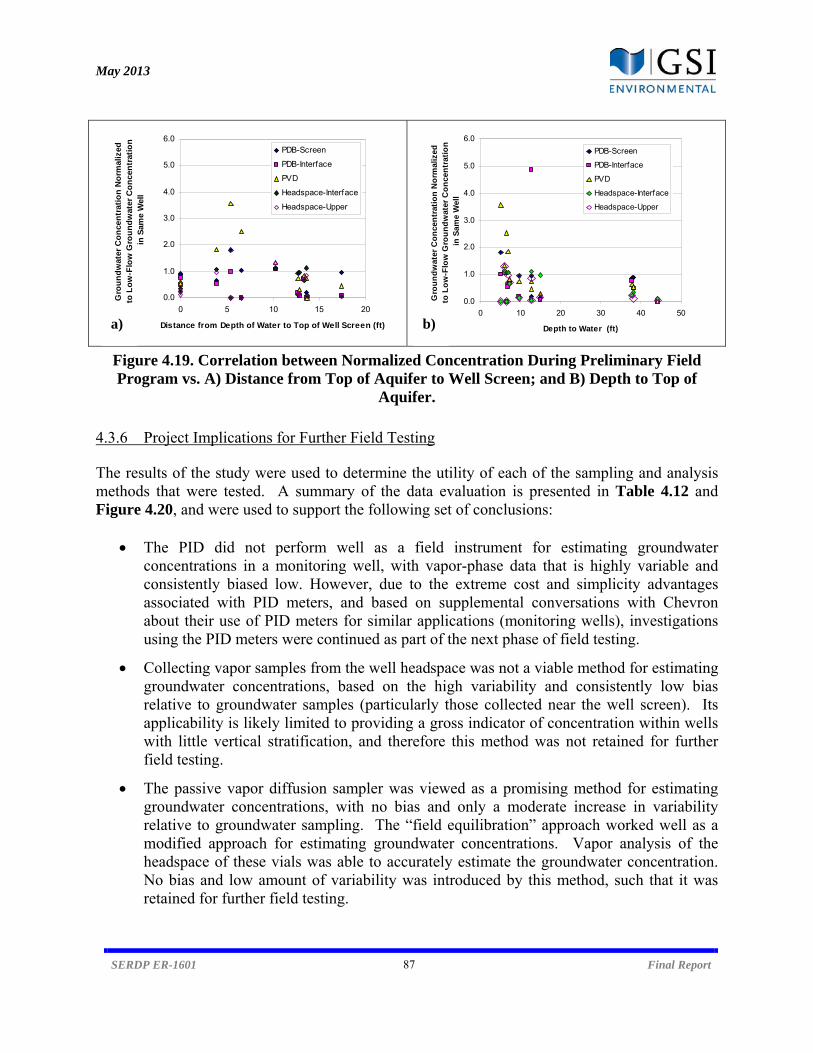
May 2013
SERDP ER-1601 87 Final Report
Figure 4.19. Correlation between Normalized Concentration During Preliminary Field Program vs. A) Distance from Top of Aquifer to Well Screen; and B) Depth to Top of
Aquifer. 4.3.6 Project Implications for Further Field Testing The results of the study were used to determine the utility of each of the sampling and analysis methods that were tested. A summary of the data evaluation is presented in Table 4.12 and Figure 4.20, and were used to support the following set of conclusions:
The PID did not perform well as a field instrument for estimating groundwater concentrations in a monitoring well, with vapor-phase data that is highly variable and consistently biased low. However, due to the extreme cost and simplicity advantages associated with PID meters, and based on supplemental conversations with Chevron about their use of PID meters for similar applications (monitoring wells), investigations using the PID meters were continued as part of the next phase of field testing.
Collecting vapor samples from the well headspace was not a viable method for estimating groundwater concentrations, based on the high variability and consistently low bias relative to groundwater samples (particularly those collected near the well screen). Its applicability is likely limited to providing a gross indicator of concentration within wells with little vertical stratification, and therefore this method was not retained for further field testing.
The passive vapor diffusion sampler was viewed as a promising method for estimating groundwater concentrations, with no bias and only a moderate increase in variability relative to groundwater sampling. The “field equilibration” approach worked well as a modified approach for estimating groundwater concentrations. Vapor analysis of the headspace of these vials was able to accurately estimate the groundwater concentration. No bias and low amount of variability was introduced by this method, such that it was retained for further field testing.
0.0
1.0
2.0
3.0
4.0
5.0
6.0
0 5 10 15 20
Distance from Depth of Water to Top of Well Screen (ft)
Gro
un
dw
ater
Co
nce
ntr
atio
n N
orm
aliz
ed
to L
ow
-Flo
w G
rou
nd
wat
er C
on
cen
trat
ion
in
Sam
e W
ell
PDB-Screen
PDB-Interface
PVD
Headspace-Interface
Headspace-Upper
0.0
1.0
2.0
3.0
4.0
5.0
6.0
0 10 20 30 40 50
Depth to Water (ft)
Gro
un
dw
ater
Co
nce
ntr
atio
n N
orm
aliz
ed
to L
ow
-Flo
w G
rou
nd
wat
er C
on
cen
trat
ion
in
Sam
e W
ell
PDB-Screen
PDB-Interface
PVD
Headspace-Interface
Headspace-Upper
a) b)

May 2013
SERDP ER-1601 88 Final Report
Figure 4.20. Overview of Bias (Slope) and Variability (R2) Observed in Sampling Methods During Preliminary Field Program.
A) Correlations with low-flow groundwater samples; and B) Inter-method correlations. PDB = passive diffusion bag (collecting groundwater); PVD = passive vapor diffusion sampler (collecting vapor).
A) B)
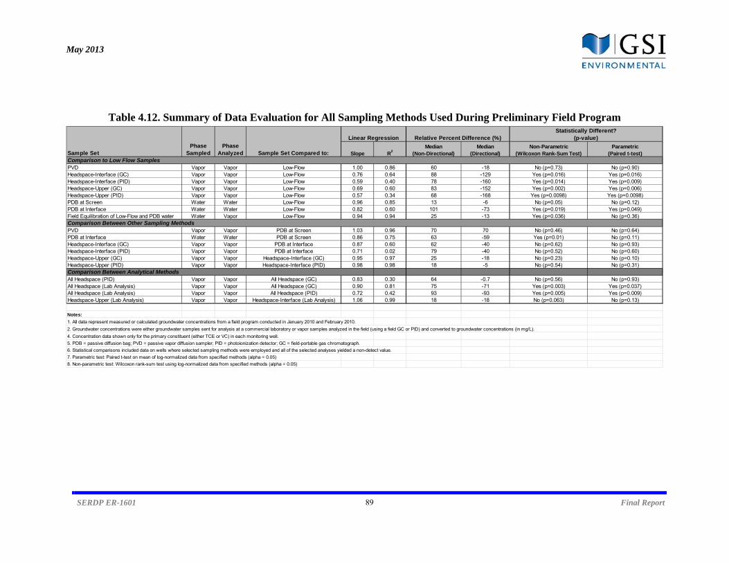
May 2013
SERDP ER-1601 89 Final Report
Table 4.12. Summary of Data Evaluation for All Sampling Methods Used During Preliminary Field Program
PVD Vapor Vapor Low-Flow 1.00 0.86 60 -18 No (p=0.73) No (p=0.90)Headspace-Interface (GC) Vapor Vapor Low-Flow 0.76 0.64 88 -129 Yes (p=0.016) Yes (p=0.016)Headspace-Interface (PID) Vapor Vapor Low-Flow 0.59 0.40 78 -160 Yes (p=0.014) Yes (p=0.009)Headspace-Upper (GC) Vapor Vapor Low-Flow 0.69 0.60 83 -152 Yes (p=0.002) Yes (p=0.006)Headspace-Upper (PID) Vapor Vapor Low-Flow 0.57 0.34 68 -168 Yes (p=0.0098) Yes (p=0.0098)PDB at Screen Water Water Low-Flow 0.96 0.85 13 -6 No (p=0.05) No (p=0.12)PDB at Interface Water Water Low-Flow 0.82 0.60 101 -73 Yes (p=0.019) Yes (p=0.049)Field Equilibration of Low-Flow and PDB water Water Vapor Low-Flow 0.94 0.94 25 -13 Yes (p=0.036) No (p=0.36)
PVD Vapor Vapor PDB at Screen 1.03 0.96 70 70 No (p=0.46) No (p=0.64)PDB at Interface Water Water PDB at Screen 0.86 0.75 63 -59 Yes (p=0.01) No (p=0.11)Headspace-Interface (GC) Vapor Vapor PDB at Interface 0.87 0.60 62 -40 No (p=0.62) No (p=0.93)Headspace-Interface (PID) Vapor Vapor PDB at Interface 0.71 0.02 79 -40 No (p=0.52) No (p=0.60)Headspace-Upper (GC) Vapor Vapor Headspace-Interface (GC) 0.95 0.97 25 -18 No (p=0.23) No (p=0.10)Headspace-Upper (PID) Vapor Vapor Headspace-Interface (PID) 0.98 0.98 18 -5 No (p=0.54) No (p=0.31)
All Headspace (PID) Vapor Vapor All Headspace (GC) 0.83 0.30 64 -0.7 No (p=0.56) No (p=0.93)All Headspace (Lab Analysis) Vapor Vapor All Headspace (GC) 0.90 0.81 75 -71 Yes (p=0.003) Yes (p=0.037)All Headspace (Lab Analysis) Vapor Vapor All Headspace (PID) 0.72 0.42 93 -93 Yes (p=0.005) Yes (p=0.009)Headspace-Upper (Lab Analysis) Vapor Vapor Headspace-Interface (Lab Analysis) 1.06 0.99 18 -18 No (p=0.063) No (p=0.13)
Notes:
1. All data represent measured or calculated groundwater concentrations from a field program conducted in January 2010 and February 2010.
2. Groundwater concentrations were either groundwater samples sent for analysis at a commercial laboratory or vapor samples analyzed in the field (using a field GC or PID) and converted to groundwater concentrations (in mg/L).
4. Concentration data shown only for the primary constituent (either TCE or VC) in each monitoring well.
5. PDB = passive diffusion bag; PVD = passive vapor diffusion sampler; PID = photoionization detector; GC = field-portable gas chromatograph.
6. Statistical comparisons included data on wells where selected sampling methods were employed and all of the selected analyses yielded a non-detect value.
7. Parametric test: Paired t-test on mean of log-normalized data from specified methods (alpha = 0.05)
8. Non-parametric test: Wilcoxon rank-sum test using log-normalized data from specified methods (alpha = 0.05)
Sample Set Sample Set Compared to:Phase
Sampled
Statistically Different?(p-value)Linear Regression
Non-Parametric(Wilcoxon Rank-Sum Test)
Parametric(Paired t-test)
Relative Percent Difference (%)
R2
Median (Directional)
Median(Non-Directional)Slope
Comparison to Low Flow Samples
Comparison Between Other Sampling Methods
Comparison Between Analytical Methods
Phase Analyzed
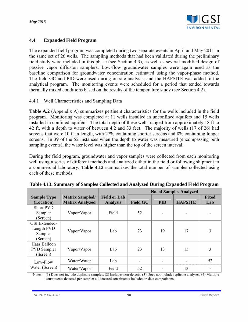
May 2013
SERDP ER-1601 90 Final Report
4.4 Expanded Field Program The expanded field program was completed during two separate events in April and May 2011 in the same set of 26 wells. The sampling methods that had been validated during the preliminary field study were included in this phase (see Section 4.3), as well as several modified design of passive vapor diffusion samplers. Low-flow groundwater samples were again used as the baseline comparison for groundwater concentration estimated using the vapor-phase method. The field GC and PID were used during on-site analysis, and the HAPSITE was added to the analytical program. The monitoring events were scheduled for a period that tended towards thermally mixed conditions based on the results of the temperature study (see Section 4.2). 4.4.1 Well Characteristics and Sampling Data Table A.2 (Appendix A) summarizes pertinent characteristics for the wells included in the field program. Monitoring was completed at 11 wells installed in unconfined aquifers and 15 wells installed in confined aquifers. The total depth of these wells ranged from approximately 18 ft to 42 ft, with a depth to water of between 4.2 and 33 feet. The majority of wells (17 of 26) had screens that were 10 ft in length, with 27% containing shorter screens and 8% containing longer screens. In 39 of the 52 instances when the depth to water was measured (encompassing both sampling events), the water level was higher than the top of the screen interval. During the field program, groundwater and vapor samples were collected from each monitoring well using a series of different methods and analyzed either in the field or following shipment to a commercial laboratory. Table 4.13 summarizes the total number of samples collected using each of these methods. Table 4.13. Summary of Samples Collected and Analyzed During Expanded Field Program
Sample Type (Location)
Matrix Sampled/ Matrix Analyzed
Field or Lab Analysis
No. of Samples Analyzed
Field GC PID HAPSITE Fixed Lab
Short PVD Sampler (Screen)
Vapor/Vapor Field 52 - - -
GSI Extended-Length PVD
Sampler (Screen)
Vapor/Vapor Lab 23 19 17 3
Haas Balloon PVD Sampler
(Screen) Vapor/Vapor Lab 23 13 15 3
Low-Flow Water (Screen)
Water/Water Lab - - - 52
Water/Vapor Field 52 - 13 - Notes: (1) Does not include duplicate samples; (2) Includes non-detects; (3) Does not include replicate analyses; (4) Multiple
constituents detected per sample; all detected constituents included in data comparisons.

May 2013
SERDP ER-1601 91 Final Report
A total of 285 sample analyses were performed as part of the field program, not including replicates. For the primary sampling methods, there were a small number of planned samples that were not collected for the following reasons:
One or more pieces of equipment were compromised (e.g., collapsed, leaking) in several wells during the first and second sampling events.
To facilitate comparisons between the vapor-based methods and conventional groundwater sampling and analysis, vapor concentrations of all detected constituents were converted to groundwater concentrations using the procedure outlined in Section 3.5. For this set of wells, this included TCE, PCE, vinyl chloride, and 1,1-DCE; one of more of these four constituents were present in each of the 26 wells included in the sampling program. The resulting groundwater concentration data are summarized in Table A.3 in Appendix A, and the raw vapor concentration data are included in Table A.4. A test for normality (Anderson-Darling) was performed on all datasets. In all cases, concentration data spanned several orders of magnitude, and the results of these tests confirmed expectations that they did not represent normal distributions. To improve the normality of this datasets—and thus improve the power of the statistical methods used to evaluate the data—log transformations were performed, and the Anderson-Darling test was re-run on the transformed data. Log transformation did not result in normally distributed data based on the test protocol (p < 0.05) except for select datasets. However, in all cases, log transformation improved the normality relative to non-transformed data (i.e., lowered the value of the test statistic). Therefore, log-transformed data were used in all subsequent evaluations of the data. 4.4.2 Comparison of Passive Vapor Diffusion Sampling to Low-Flow Groundwater Sampling Comparisons were performed between groundwater concentration data calculated using field measurements of equilibrium vapor samples and groundwater concentration data measured using lab analysis of low-flow groundwater samples. Results of these comparisons are presented for the following evaluations:
i) Linear regression, using the correlation coefficient (R2) as an indicator of variability and the slope as an indicator of bias. Paired data comparisons for all constituents present in each individual well were included in the regressions. Note that in addition to being presented and discussed in the following section, all linear regression plots from this phase of field testing are included in Figure A.2 of Appendix A for easy comparison.
ii) Two-sample tests (parametric and non-parametric) to determine if there is a statistically-significant difference between the means of the low-flow groundwater data and the groundwater data calculated using the vapor-phase based methods.
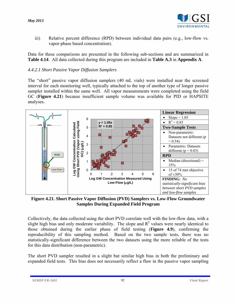
May 2013
SERDP ER-1601 92 Final Report
iii) Relative percent difference (RPD) between individual data pairs (e.g., low-flow vs. vapor-phase based concentration).
Data for these comparisons are presented in the following sub-sections and are summarized in Table 4.14. All data collected during this program are included in Table A.3 in Appendix A. 4.4.2.1 Short Passive Vapor Diffusion Samplers The “short” passive vapor diffusion samplers (40 mL vials) were installed near the screened interval for each monitoring well, typically attached to the top of another type of longer passive sampler installed within the same well. All vapor measurements were completed using the field GC (Figure 4.21) because insufficient sample volume was available for PID or HAPSITE analyses.
Linear Regression Slope = 1.05 R2 = 0.85 Two-Sample Tests Non-parametric:
Datasets not different (p = 0.54)
Parametric: Datasets different (p = 0.03)
RPD Median (directional) =
35% 15 of 74 met objective
of ±30% FINDING: No statistically-significant bias between short PVD samples and low-flow samples
Figure 4.21. Short Passive Vapor Diffusion (PVD) Samplers vs. Low-Flow Groundwater Samples During Expanded Field Program
Collectively, the data collected using the short PVD correlate well with the low-flow data, with a slight high bias and only moderate variability. The slope and R2 values were nearly identical to those obtained during the earlier phase of field testing (Figure 4.9), confirming the reproducibility of this sampling method. Based on the two sample tests, there was no statistically-significant difference between the two datasets using the more reliable of the tests for this data distribution (non-parametric). The short PVD sampler resulted in a slight but similar high bias in both the preliminary and expanded field tests. This bias does not necessarily reflect a flaw in the passive vapor sampling
y = 1.05xR² = 0.85
0
1
2
3
4
5
6
0 1 2 3 4 5 6Lo
g G
W C
on
cen
trat
ion
Cal
cula
ted
U
sin
g S
ho
rt P
VD
(V
apo
r u
sin
g F
ield
G
C)
(g
/L)
Log GW Concentration Measured Using Low-Flow (g/L)
PVD
Low-Flow
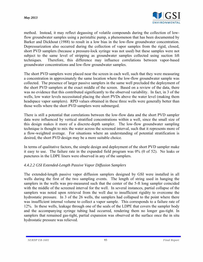
May 2013
SERDP ER-1601 93 Final Report
method. Instead, it may reflect degassing of volatile compounds during the collection of low-flow groundwater samples using a peristaltic pump, a phenomenon that has been documented by Barker and Dickhout (1988) to result in a low bias in the low-flow groundwater concentration. Depressurization also occurred during the collection of vapor samples from the rigid, closed, short PVD samplers (because a pressure-lock syringe was not used) but these samples were not subject to the same level of stripping as groundwater samples collected using suction lift techniques. Therefore, this difference may influence correlations between vapor-based groundwater concentrations and low-flow groundwater samples. The short PVD samplers were placed near the screen in each well, such that they were measuring a concentration in approximately the same location where the low-flow groundwater sample was collected. The presence of larger passive samplers in the same well precluded the deployment of the short PVD samplers at the exact middle of the screen. Based on a review of the data, there was no evidence that this contributed significantly to the observed variability. In fact, in 3 of the wells, low water levels necessitated placing the short PVDs above the water level (making them headspace vapor samplers). RPD values obtained in these three wells were generally better than those wells where the short PVD samplers were submerged. There is still a potential that correlations between the low-flow data and the short PVD sampler data were influenced by vertical stratified concentrations within a well, since the small size of this design makes it more of a discrete-depth sampler. The low-flow groundwater sampling technique is thought to mix the water across the screened interval, such that it represents more of a flow-weighted average. For situations where an understanding of potential stratification is desired, the short PVD design may be a more suitable choice. In terms of qualitative factors, the simple design and deployment of the short PVD sampler make it easy to use. The failure rate in the expanded field program was 0% (0 of 52). No leaks or punctures in the LDPE liners were observed in any of the samplers. 4.4.2.2 GSI Extended-Length Passive Vapor Diffusion Samplers The extended-length passive vapor diffusion samplers designed by GSI were installed in all wells during the first of the two sampling events. The length of string used in hanging the samplers in the wells was pre-measured such that the center of the 5-ft long sampler coincided with the middle of the screened interval for the well. In several instances, partial collapse of the samplers was noted upon retrieval from the well due to insufficient rigidity to overcome the hydrostatic pressure. In 3 of the 26 wells, the samplers had collapsed to the point where there was insufficient internal volume to collect a vapor sample. This corresponds to a failure rate of 12%. In these wells, leakage through one of the seals of the LDPE that covers the sampler body and the accompanying syringe tubing had occurred, rendering them no longer gas-tight. In samplers that remained gas-tight, partial expansion was observed at the surface once the in situ hydrostatic pressure was relieved.
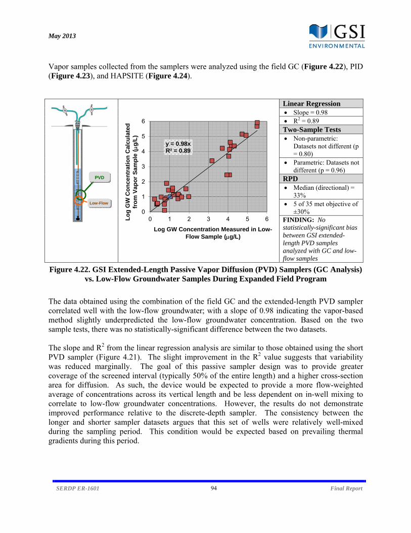
May 2013
SERDP ER-1601 94 Final Report
Vapor samples collected from the samplers were analyzed using the field GC (Figure 4.22), PID (Figure 4.23), and HAPSITE (Figure 4.24).
Linear Regression Slope = 0.98 R2 = 0.89 Two-Sample Tests Non-parametric:
Datasets not different (p = 0.80)
Parametric: Datasets not different (p = 0.96)
RPD Median (directional) =
33% 5 of 35 met objective of
±30% FINDING: No statistically-significant bias between GSI extended-length PVD samples analyzed with GC and low-flow samples
Figure 4.22. GSI Extended-Length Passive Vapor Diffusion (PVD) Samplers (GC Analysis) vs. Low-Flow Groundwater Samples During Expanded Field Program
The data obtained using the combination of the field GC and the extended-length PVD sampler correlated well with the low-flow groundwater; with a slope of 0.98 indicating the vapor-based method slightly underpredicted the low-flow groundwater concentration. Based on the two sample tests, there was no statistically-significant difference between the two datasets. The slope and R2 from the linear regression analysis are similar to those obtained using the short PVD sampler (Figure 4.21). The slight improvement in the R2 value suggests that variability was reduced marginally. The goal of this passive sampler design was to provide greater coverage of the screened interval (typically 50% of the entire length) and a higher cross-section area for diffusion. As such, the device would be expected to provide a more flow-weighted average of concentrations across its vertical length and be less dependent on in-well mixing to correlate to low-flow groundwater concentrations. However, the results do not demonstrate improved performance relative to the discrete-depth sampler. The consistency between the longer and shorter sampler datasets argues that this set of wells were relatively well-mixed during the sampling period. This condition would be expected based on prevailing thermal gradients during this period.
y = 0.98xR² = 0.89
0
1
2
3
4
5
6
0 1 2 3 4 5 6Lo
g G
W C
on
cen
trat
ion
Cal
cula
ted
fr
om
Vap
or
Sam
ple
(g
/L)
Log GW Concentration Measured in Low-Flow Sample (g/L)
PVD
Low-Flow

May 2013
SERDP ER-1601 95 Final Report
Based on its design, the extended-length PVD is allowed to expand after it is retrieved from a well and is no longer subject to hydrostatic pressure. Its strong performance demonstrated that the pressure corrections employed in calculating the equivalent groundwater concentration were sufficient to account for this factor.
Linear Regression Slope = 0.83 R2 = 0.55 Two-Sample Tests Non-parametric:
Datasets not different (p = 0.51)
Parametric: Datasets not different (p = 0.06)
RPD Median (directional) =
-82% 6 of 55 met objective of
±30% FINDING: Differences between GSI extended-length PVD samples analyzed with PID and low-flow samples (low bias), though not statistically significant
Figure 4.23. GSI Extended-Length Passive Vapor Diffusion (PVD) Samplers (PID Analysis) vs. Low-Flow Groundwater Samples During Expanded Field Program
The data obtained using PID analyses and the extended-length sampler were poor relative to those obtained using the field GC. The results were biased low with a higher level of variability, particularly at lower-end of the concentration range. The PID and low-flow datasets were not different based on the statistical significance tests using a 95% level of significance, though they would have been different if at the 90% level based on the parametric test. Because the PID uses a single signal response to represent all constituents present, it is more difficult to reliably convert this value to an estimated groundwater concentration. In effect, the expected ratio of the constituents must be known beforehand and used in conjunction with constituent-specific correction factors supplied by the instrument’s manufacturer. These factors likely contribute to the observed variability in the data, though they do not necessarily explain the low bias seen here. Linear regression analyses were repeated using data for individual constituents rather than datasets where all constituents were grouped together (as in Figure 4.23). The results of these comparisons (not shown), demonstrate a slight reduction in variability for most constituents. This includes a higher R2 values for VC, which was typically the
y = 0.83xR² = 0.55
0
1
2
3
4
5
6
-1 0 1 2 3 4 5 6Lo
g G
W C
on
cen
trat
ion
Cal
cula
ted
U
sin
g E
xten
ded
-Le
ng
th P
VD
(V
ap
or
usi
ng
PID
) (
g/L
)
Log GW Concentration Measured Using Low-Flow (g/L)
PVD
Low-Flow
May 2013
SERDP ER-1601 96 Final Report
dominant constituent (i.e., > 90% of the total VOC concentration) when it was detected in this set of monitoring wells. Consequently, the PID appears to generate slightly more reproducible data at wells where only one constituent is present, although the results indicate that it still consistently underpredicts the low-flow groundwater concentration in these situations. Linear Regression
Slope = 0.32 R2 = 0.19 Two-Sample Tests Non-parametric:
Datasets different (p < 0.0001)
Parametric: Datasets different (p < 0.0001)
RPD Median (directional) =
-117% 5 of 43 met objective of
±30% FINDING: Statistically-significant difference between GSI extended-length PVD samples analyzed with HAPSITE and low-flow samples
Figure 4.24. GSI Extended-Length Passive Vapor Diffusion (PVD) Samplers (HAPSITE Analysis) vs. Low-Flow Groundwater Samples During Expanded Field Program
The data obtained using the HAPSITE were consistently biased low relative to the low-flow groundwater dataset, and its overall performance was not as strong as either the field GC or the PID. A high degree of variability was observed (R2 = 0.19), as illustrated by the several order-of-magnitude spread of predicted concentrations observed near the upper-end of the low-flow concentration data. Conversely, significant scatter was also observed at the lower-end of the low-flow concentration range. In part, this latter observation was attributable to the low detection limits provided by the HAPSITE. The instrument is capable of reporting concentrations that are equivalent to much less than 1 g/L (with positive identification provided by its MS capabilities). As such, it generated a larger dataset of lower-end concentrations than either the field GC or PID, but there was an apparent difficulty in obtaining strong correlations with these additional datapoints. In addition, the HAPSITE consistently underpredicted the low-flow groundwater concentrations, often by one or more orders of magnitude. The sampling and analysis plan utilized for this field program likely contributed to this problem. Specifically, the HAPSITE analyses were not performed in the field but rather were performed after all field samples were collected (in a
y = 0.32xR² = 0.19
-1
0
1
2
3
4
5
6
-1 0 1 2 3 4 5 6
Lo
g G
W C
on
cen
trat
ion
Cal
cula
ted
U
sin
g E
xten
ded
-Len
gth
PV
D (
Vap
or
usi
ng
HA
PS
ITE
) (
g/L
)
Log GW Concentration Measured Using Low-Flow (g/L)
PVD
Low-Flow
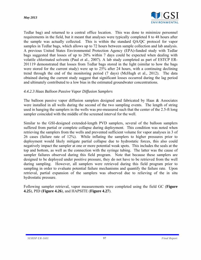
May 2013
SERDP ER-1601 97 Final Report
Tedlar bag) and returned to a central office location. This was done to minimize personnel requirements in the field, but it meant that analyses were typically completed 8 to 48 hours after the sample was actually collected. This is within the standard QA/QC protocol for vapor samples in Tedlar bags, which allows up to 72 hours between sample collection and lab analysis. A previous United States Environmental Protection Agency (EPA)-funded study with Tedlar bags suggested that losses of up to 20% within 7 days could be expected when dealing with volatile chlorinated solvents (Paul et al., 2007). A lab study completed as part of ESTCP ER-201119 demonstrated that losses from Tedlar bags stored in the light (similar to how the bags were stored for the current study) were up to 25% after 24 hours, with a continuing declining trend through the end of the monitoring period (7 days) (McHugh et al., 2012). The data obtained during the current study suggest that significant losses occurred during the lag period and ultimately contributed to a low bias in the estimated groundwater concentrations. 4.4.2.3 Haas Balloon Passive Vapor Diffusion Samplers The balloon passive vapor diffusion samplers designed and fabricated by Haas & Associates were installed in all wells during the second of the two sampling events. The length of string used in hanging the samplers in the wells was pre-measured such that the center of the 2.5-ft long sampler coincided with the middle of the screened interval for the well. Similar to the GSI-designed extended-length PVD samplers, several of the balloon samplers suffered from partial or complete collapse during deployment. This condition was noted when retrieving the samplers from the wells and prevented sufficient volume for vapor analyses in 3 of 26 cases (failure rate of 12%). While inflating the samplers to higher pressures prior to deployment would likely mitigate partial collapse due to hydrostatic forces, this also could negatively impact the sampler at one or more potential weak spots. This includes the seals at the top and bottom, as well as the connection with the syringe tubing. The latter was the cause of sampler failures observed during this field program. Note that because these samplers are designed to be deployed under positive pressure, they do not have to be retrieved from the well during sampling. However, all samplers were retrieved during this field program prior to sampling in order to evaluate potential failure mechanisms and quantify the failure rate. Upon retrieval, partial expansion of the samplers was observed due to relieving of the in situ hydrostatic pressure. Following sampler retrieval, vapor measurements were completed using the field GC (Figure 4.25), PID (Figure 4.26), and HAPSITE (Figure 4.27).
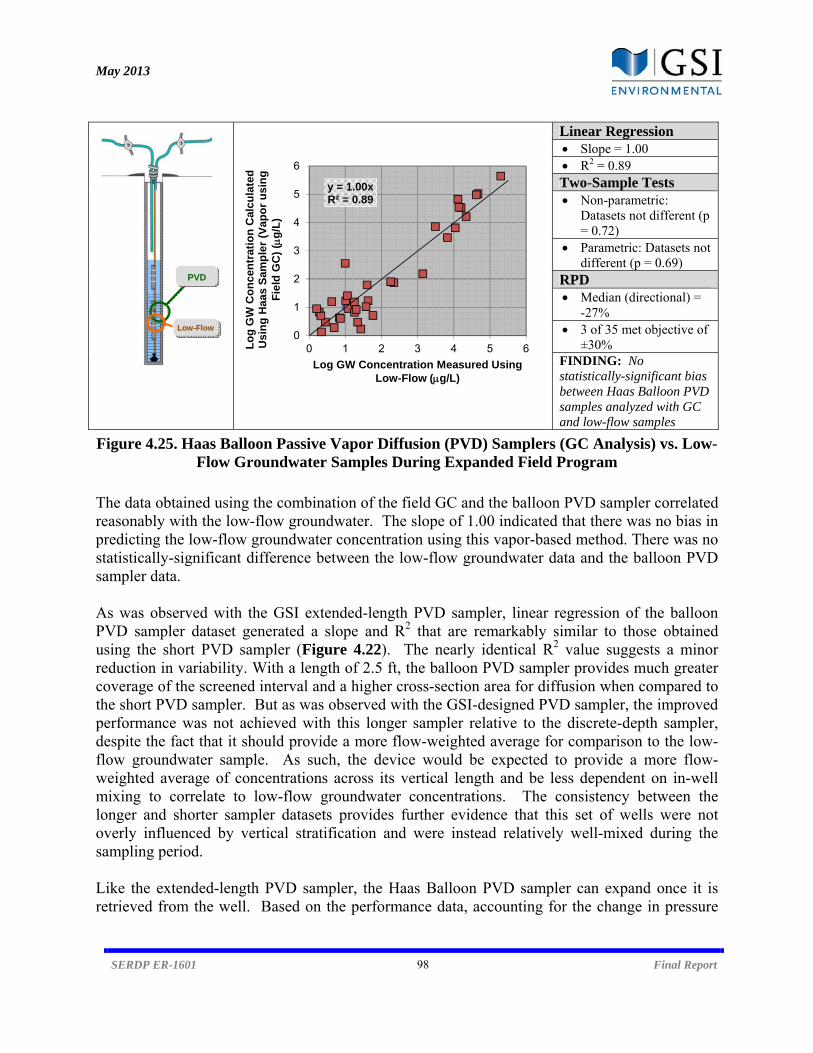
May 2013
SERDP ER-1601 98 Final Report
Linear Regression Slope = 1.00 R2 = 0.89 Two-Sample Tests Non-parametric:
Datasets not different (p = 0.72)
Parametric: Datasets not different (p = 0.69)
RPD Median (directional) =
-27% 3 of 35 met objective of
±30% FINDING: No statistically-significant bias between Haas Balloon PVD samples analyzed with GC and low-flow samples
Figure 4.25. Haas Balloon Passive Vapor Diffusion (PVD) Samplers (GC Analysis) vs. Low-Flow Groundwater Samples During Expanded Field Program
The data obtained using the combination of the field GC and the balloon PVD sampler correlated reasonably with the low-flow groundwater. The slope of 1.00 indicated that there was no bias in predicting the low-flow groundwater concentration using this vapor-based method. There was no statistically-significant difference between the low-flow groundwater data and the balloon PVD sampler data. As was observed with the GSI extended-length PVD sampler, linear regression of the balloon PVD sampler dataset generated a slope and R2 that are remarkably similar to those obtained using the short PVD sampler (Figure 4.22). The nearly identical R2 value suggests a minor reduction in variability. With a length of 2.5 ft, the balloon PVD sampler provides much greater coverage of the screened interval and a higher cross-section area for diffusion when compared to the short PVD sampler. But as was observed with the GSI-designed PVD sampler, the improved performance was not achieved with this longer sampler relative to the discrete-depth sampler, despite the fact that it should provide a more flow-weighted average for comparison to the low-flow groundwater sample. As such, the device would be expected to provide a more flow-weighted average of concentrations across its vertical length and be less dependent on in-well mixing to correlate to low-flow groundwater concentrations. The consistency between the longer and shorter sampler datasets provides further evidence that this set of wells were not overly influenced by vertical stratification and were instead relatively well-mixed during the sampling period. Like the extended-length PVD sampler, the Haas Balloon PVD sampler can expand once it is retrieved from the well. Based on the performance data, accounting for the change in pressure
y = 1.00xR² = 0.89
0
1
2
3
4
5
6
0 1 2 3 4 5 6Lo
g G
W C
on
cen
trat
ion
Cal
cula
ted
U
sin
g H
aas
Sam
ple
r (V
apo
r u
sin
g
Fie
ld G
C)
(g
/L)
Log GW Concentration Measured Using Low-Flow (g/L)
PVD
Low-Flow
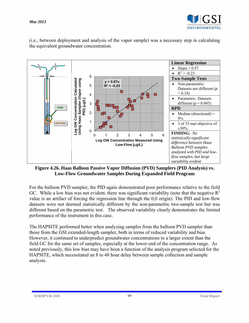
May 2013
SERDP ER-1601 99 Final Report
(i.e., between deployment and analysis of the vapor sample) was a necessary step in calculating the equivalent groundwater concentration.
Linear Regression Slope = 0.97 R2 = -0.23 Two-Sample Tests Non-parametric:
Datasets not different (p = 0.18)
Parametric: Datasets different (p = 0.045)
RPD Median (directional) =
9% 3 of 33 met objective of
±30% FINDING: No statistically-significant difference between Haas Balloon PVD samples analyzed with PID and low-flow samples, but large variability evident
Figure 4.26. Haas Balloon Passive Vapor Diffusion (PVD) Samplers (PID Analysis) vs. Low-Flow Groundwater Samples During Expanded Field Program
For the balloon PVD sampler, the PID again demonstrated poor performance relative to the field GC. While a low bias was not evident, there was significant variability (note that the negative R2 value is an artifact of forcing the regression line through the 0,0 origin). The PID and low-flow datasets were not deemed statistically different by the non-parametric two-sample test but was different based on the parametric test. The observed variability clearly demonstrates the limited performance of the instrument in this case. The HAPSITE performed better when analyzing samples from the balloon PVD sampler than those from the GSI extended-length sampler, both in terms of reduced variability and bias. However, it continued to underpredict groundwater concentrations to a larger extent than the field GC for the same set of samples, especially at the lower-end of the concentration range. As noted previously, this low bias may have been a function of the analysis program selected for the HAPSITE, which necessitated an 8 to 48 hour delay between sample collection and sample analysis.
y = 0.97xR² = -0.23
0
1
2
3
4
5
6
0 1 2 3 4 5 6Lo
g G
W C
on
cen
trat
ion
Cal
cula
ted
U
sin
g H
aas
Sam
ple
r (V
apo
r u
sin
g
PID
) (
g/L
)
Log GW Concentration Measured Using Low-Flow (g/L)
PVD
Low-Flow
May 2013
SERDP ER-1601 100 Final Report
Linear Regression Slope = 0.82 R2 = 0.84 Two-Sample Tests Non-parametric:
Datasets different (p=0.015)
Parametric: Datasets different (p < 0.0001)
RPD Median (directional) =
-100% 3 of 28 met objective of
±30% FINDING: Statistically-significant difference between Haas Balloon PVD samples analyzed with HAPSITE and low-flow samples
Figure 4.27. Haas Balloon Passive Vapor Diffusion (PVD) Samplers (HAPSITE Analysis) vs. Low-Flow Groundwater Samples During Expanded Field Program
4.4.3 Field Analysis of Groundwater Samples (Field Equilibration Method) The alternate “field equilibration” method for determining groundwater concentrations was investigated at all locations by placing a water sample from the well in a sealed vial (for small volume analyses) or Tedlar bag (for larger volume analyses) containing a headspace and agitating the sample for a sufficient period of time to achieve equilibrium partitioning. The field GC was used to analyze the vapor in the headspace of 40-mL vials, while the HAPSITE required higher volumes and used the vapor in the partially-filled Tedlar bags. For all instruments, the vapor result was converted to a VOC concentration in the water sample. This method was employed for all low-flow groundwater samples collected during the expanded field program. The groundwater concentrations calculated using the vapor-phase field measurements were then compared to the concentrations measured when the corresponding groundwater samples were analyzed off-site at a commercial lab (Figure 4.28).
y = 0.82xR² = 0.84
0
1
2
3
4
5
6
0 1 2 3 4 5 6Lo
g G
W C
on
cen
trat
ion
Cal
cula
ted
U
sin
g H
aas
Sam
ple
r (V
apo
r u
sin
g
HA
PS
ITE
) (
g/L
)
Log GW Concentration Measured Using Low-Flow (g/L)
PVD
Low-Flow

May 2013
SERDP ER-1601 101 Final Report
Linear Regression Slope = 1.01 R2 = 0.97 Two-Sample Tests Non-parametric:
Datasets not different (p=0.78)
Parametric: Datasets not different (p=0.98)
RPD Median (directional) =
3% 34 of 74 met objective
of ±30% FINDING: No statistically-significant difference between lab analysis of groundwater samples and field GC analysis of vapor in equilibrium with low-flow groundwater sample
Figure 4.28. Field GC Analysis of Vapor in Equilibrium with Groundwater Samples vs. Lab Analysis of Groundwater Samples During Expanded Field Program
Linear Regression Slope = 0.74 R2 = 0.71 Two-Sample Tests Non-parametric:
Datasets different (p < 0.0001)
Parametric: Datasets different (p < 0.0001)
RPD Median (directional) =
-135% 0 of 29 met objective of
±30% FINDING: Statistically-significant difference between lab analysis of groundwater samples and field HAPSITE analysis of vapor in equilibrium with low-flow groundwater sample
Figure 4.29. Field HAPSITE Analysis of Vapor in Equilibrium with Groundwater Samples vs. Lab Analysis of Groundwater Samples During Expanded Field Program
y = 1.01xR² = 0.97
0
1
2
3
4
5
6
0 1 2 3 4 5 6
Lo
g G
W C
on
cen
trat
ion
Cal
cula
ted
U
sin
g F
ield
Vap
or
An
alys
is o
f E
qu
ilib
riu
m G
rou
nd
wat
er (
Vap
or
usi
ng
Fie
ld G
C)
(g
/L)
Log GW Concentration Measured Using Low-Flow (g/L)
y = 0.74xR² = 0.71
0
1
2
3
4
5
6
0 1 2 3 4 5 6
Lo
g G
W C
on
cen
trat
ion
Cal
cula
ted
U
sin
g F
ield
Vap
or
An
alys
is o
f E
qu
ilib
riu
m G
rou
nd
wat
er (
Vap
or
usi
ng
HA
PS
ITE
) (
g/L
)
Log GW Concentration Measured Using Low-Flow (g/L)
Low-flow or PDB
Analyze vapor in field
Low-flow or PDB
Analyze vapor in field

May 2013
SERDP ER-1601 102 Final Report
The results obtained using the field GC demonstrated that this sampling and analysis method was consistently able to match expected groundwater concentrations, with no bias and very little variability. Because the method involves collecting a low-flow groundwater sample, it is not influenced by well and aquifer characteristics in the same way that the passive vapor samplers are. Instead, it serves as a good representation of the bias and/or variability associated with the field analysis. This includes any bias or variability introduced during i) transfer of the water sample to the 40-mL vial; ii) the equilibrium period; iii) the analysis of the vapor using the GC; and iv) conversion of the vapor concentration to an equivalent groundwater concentration. Given the strong agreement between the field equilibration dataset obtained using the field GC and the low-flow dataset, it appears that none of these steps significantly impact the comparison. Using the HAPSITE to analyze these samples, a low bias was evident along with a significant level of variability (Figure 4.29). This trend is consistent with that obtained when HAPSITE data was collected using passive vapor diffusion samplers. Overall, the data are similar to those obtained during the preliminary field program and confirm the utility of the field equilibration approach for estimating groundwater concentrations. 4.4.4 Comparison of Individual Vapor-Phase Based Sampling Methods To compare data obtained using each of the individual vapor-phase based sampling methods, the same quantitative approaches were used: i) linear regression; ii) two sample tests; and iii) relative percent difference. The following paired datasets were compared:
GSI Extended-Length PVD to Short PVD (GC analysis) Haas Balloon PVD to Short PVD (GC analysis) Field Equilibration of Low-Flow Groundwater to GSI Extended-Length PVD (GC
Analysis) Field Equilibration of Low-Flow Groundwater to Haas Balloon PVD (GC Analysis) Field Equilibration of Low-Flow Groundwater to Short PVD (GC Analysis)
The results of these comparisons are summarized in Table 4.14, with the regression analyses shown in Figure A.3 of Appendix A. Note that a direct comparison between the GSI extended-length PVD dataset and the Haas balloon PVD dataset could not be made because these devices were deployed during different sampling events. Given the significant inter-event differences between concentrations obtained using low-flow groundwater sampling (see Section 4.4.5), this would not have been a true “apples-to-apples” comparison. In general, there was a strong degree of correlation between each of the paired datasets obtained with the field GC, with little or no bias evident (slope = 0.89 to 1.00). The range of variability was low (R2 = 0.85 to 0.95) and was similar to the range obtained when the datasets were

May 2013
SERDP ER-1601 103 Final Report
compared with low-flow groundwater concentration data. In addition, there were few indications that any of the datasets were statistically significantly different from each other (particularly using the non-parametric tests). The consistency between the datasets supports the argument that any of the vapor-phase based methods would be expected to perform similarly when estimating low-flow groundwater concentrations. 4.4.5 Evaluation of Precision and Accuracy for Field and Lab Analyses Several other methods were employed to investigate the precision and accuracy of the various sampling and analyses methods.
4.4.5.1 Laboratory and Field Analyses of Replicate Samples Groundwater replicate (duplicate) samples were collected for analysis at commercial laboratories as part of this phase of field testing. For each set of duplicates, the relative standard deviation (RSD) was calculated as a metric for assessing precision (Table 4.15).
Table 4.15. Precision of Laboratory vs. Field Analyses of Duplicate Samples During Expanded Field Program
Analysis Type No. of Duplicate
Sample Sets RSD (%)
Range Median Groundwater (Lab) 17 0.0 – 38 % 5.3 %
The level of precision for lab analyses of duplicates was similar to that obtained during the earlier phase of field testing. Note that the RSD values in Table 4.15 reflect variability associated with the sampling steps as well as the analysis steps.
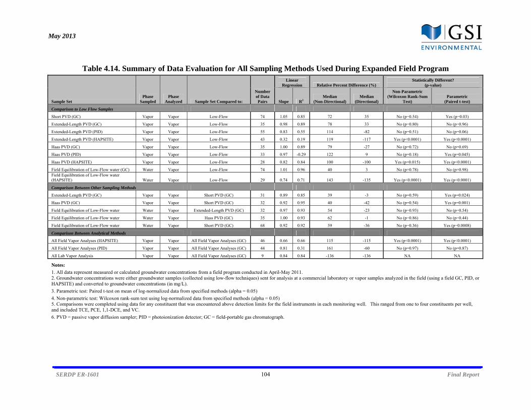
May 2013
SERDP ER-1601 104 Final Report
Table 4.14. Summary of Data Evaluation for All Sampling Methods Used During Expanded Field Program
Sample Set Phase
Sampled Phase
Analyzed Sample Set Compared to:
Number of Data Pairs
Linear Regression Relative Percent Difference (%)
Statistically Different? (p-value)
Slope R2 Median
(Non-Directional) Median
(Directional)
Non-Parametric (Wilcoxon Rank-Sum
Test) Parametric
(Paired t-test)
Comparison to Low Flow Samples
Short PVD (GC) Vapor Vapor Low-Flow 74 1.05 0.85 72 35 No (p=0.54) Yes (p=0.03)
Extended-Length PVD (GC) Vapor Vapor Low-Flow 35 0.98 0.89 78 33 No (p=0.80) No (p=0.96)
Extended-Length PVD (PID) Vapor Vapor Low-Flow 55 0.83 0.55 114 -82 No (p=0.51) No (p=0.06)
Extended-Length PVD (HAPSITE) Vapor Vapor Low-Flow 43 0.32 0.19 119 -117 Yes (p<0.0001) Yes (p<0.0001)
Haas PVD (GC) Vapor Vapor Low-Flow 35 1.00 0.89 79 -27 No (p=0.72) No (p=0.69)
Haas PVD (PID) Vapor Vapor Low-Flow 33 0.97 -0.29 122 9 No (p=0.18) Yes (p=0.045)
Haas PVD (HAPSITE) Vapor Vapor Low-Flow 28 0.82 0.84 100 -100 Yes (p=0.015) Yes (p<0.0001)
Field Equilibration of Low-Flow water (GC) Water Vapor Low-Flow 74 1.01 0.96 40 3 No (p=0.78) No (p=0.98) Field Equilibration of Low-Flow water (HAPSITE) Water Vapor Low-Flow 29 0.74 0.71 143 -135 Yes (p<0.0001) Yes (p<0.0001)
Comparison Between Other Sampling Methods
Extended-Length PVD (GC) Vapor Vapor Short PVD (GC) 31 0.89 0.85 39 -3 No (p=0.59) Yes (p=0.024)
Haas PVD (GC) Vapor Vapor Short PVD (GC) 32 0.92 0.95 40 -42 No (p=0.54) Yes (p=0.001)
Field Equilibration of Low-Flow water Water Vapor Extended-Length PVD (GC) 32 0.97 0.93 54 -23 No (p=0.93) No (p=0.54)
Field Equilibration of Low-Flow water Water Vapor Hass PVD (GC) 35 1.00 0.93 62 -1 No (p=0.86) No (p=0.44)
Field Equilibration of Low-Flow water Water Vapor Short PVD (GC) 68 0.92 0.92 59 -36 No (p=0.36) Yes (p=0.0008)
Comparison Between Analytical Methods
All Field Vapor Analyses (HAPSITE) Vapor Vapor All Field Vapor Analyses (GC) 46 0.66 0.66 115 -115 Yes (p<0.0001) Yes (p<0.0001)
All Field Vapor Analyses (PID) Vapor Vapor All Field Vapor Analyses (GC) 44 0.81 0.31 161 -60 No (p=0.97) No (p=0.87)
All Lab Vapor Analysis Vapor Vapor All Field Vapor Analyses (GC) 9 0.84 0.84 -136 -136 NA NA
Notes: 1. All data represent measured or calculated groundwater concentrations from a field program conducted in April-May 2011. 2. Groundwater concentrations were either groundwater samples (collected using low-flow techniques) sent for analysis at a commercial laboratory or vapor samples analyzed in the field (using a field GC, PID, or HAPSITE) and converted to groundwater concentrations (in mg/L).
3. Parametric test: Paired t-test on mean of log-normalized data from specified methods (alpha = 0.05)
4. Non-parametric test: Wilcoxon rank-sum test using log-normalized data from specified methods (alpha = 0.05) 5. Comparisons were completed using data for any constituent that was encountered above detection limits for the field instruments in each monitoring well. This ranged from one to four constituents per well, and included TCE, PCE, 1,1-DCE, and VC.
6. PVD = passive vapor diffusion sampler; PID = photoionization detector; GC = field-portable gas chromatograph.
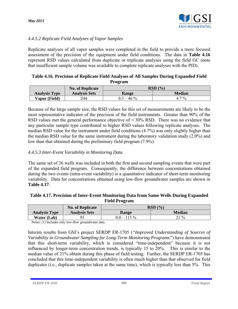
May 2013
SERDP ER-1601 105 Final Report
4.4.5.2 Replicate Field Analyses of Vapor Samples Replicate analyses of all vapor samples were completed in the field to provide a more focused assessment of the precision of the equipment under field conditions. The data in Table 4.16 represent RSD values calculated from duplicate or triplicate analyses using the field GC (note that insufficient sample volume was available to complete replicate analyses with the PID).
Table 4.16. Precision of Replicate Field Analyses of All Samples During Expanded Field Program
Analysis Type No. of Replicate
Analysis Sets RSD (%)
Range Median Vapor (Field) 244 0.3 – 46 % 4.7 %
Because of the large sample size, the RSD values for this set of measurements are likely to be the most representative indicator of the precision of the field instruments. Greater than 90% of the RSD values met the general performance objective of < 30% RSD. There was no evidence that any particular sample type contributed to higher RSD values following replicate analyses. The median RSD value for the instrument under field conditions (4.7%) was only slightly higher than the median RSD value for the same instrument during the laboratory validation study (2.0%) and low than that obtained during the preliminary field program (7.9%). 4.4.5.3 Inter-Event Variability in Monitoring Data The same set of 26 wells was included in both the first and second sampling events that were part of the expanded field program. Consequently, the difference between concentrations obtained during the two events (intra-event variability) is a quantitative indicator of short-term monitoring variability. Data for concentrations obtained using low-flow groundwater samples are shown in Table 4.17: Table 4.17. Precision of Inter-Event Monitoring Data from Same Wells During Expanded
Field Program
Analysis Type No. of Replicate
Analysis Sets RSD (%)
Range Median Water (Lab) 93 0.0 – 113 % 21 %
Notes: (1) Includes only low-flow groundwater data.
Interim results from GSI’s project SERDP ER-1705 (“Improved Understanding of Sources of Variability in Groundwater Sampling for Long-Term Monitoring Programs”) have demonstrated that this short-term variability, which is considered “time-independent” because it is not influenced by longer-term concentration trends, is typically 15 to 20%. This is similar to the median value of 21% obtain during this phase of field testing. Further, the SERDP ER-1705 has concluded that this time-independent variability is often much higher than that observed for field duplicates (i.e., duplicate samples taken at the same time), which is typically less than 5%. This

May 2013
SERDP ER-1601 106 Final Report
is consistent with the variability observed for field duplicates during the expanded field study (4.7%). Collectively, these data illustrate that short-term variability is an inherent limitation in interpreting monitoring data, regardless of whether it is collected using conventional or innovative (e.g., vapor-phase based) methods. Reducing this short-term variability was an objective of the supplemental field program that was conducted in conjunction with subsequent SERDP ER-1705 field testing (see Section 4.5) 4.4.5.4 Field GC vs. PID Analyses of Vapor Samples For those wells where vapor samples were analyzed by both the field GC and the PID, the resulting data was used to determine potential bias in either of the field instruments (Figure 4.30, Table 4.14). For each instrument, all data was lumped together, regardless of which sampling device was used to collect the data.
Figure 4.30. Field PID Analyses vs. Field GC Analyses of Samples Collected During
Expanded Field Program
Using this bulk comparison, it appeared that the PID provided a relatively good correlation with field GC measurements at high vapor concentrations (albeit with a low bias), but that the correlation became poorer at low concentrations. For example, there were a large number of detections in the lower-end of the field GC dataset that were biased high when analyzed by the PID. This differed from the relationship seen in the results of the preliminary field program (i.e., better correlation at low concentrations), but was aided by the fact that PID samples were frequently diluted prior to analyses to avoid the relatively low upper detection limit for the instrument. Regardless, considerable variability was again observed (R2=0.31) between the data collected using the two analytical instruments. This variability is generally consistent with that
y = 0.81xR² = 0.31
0
1
2
3
4
5
6
0 1 2 3 4 5 6
Lo
g G
W C
on
cen
trat
ion
Cal
cula
ted
U
sin
g V
apo
r A
nal
yzed
wit
h P
ID
(g
/L)
Log GW Concentration Calcuated Using Vapor Analyzed with Field GC (g/L)
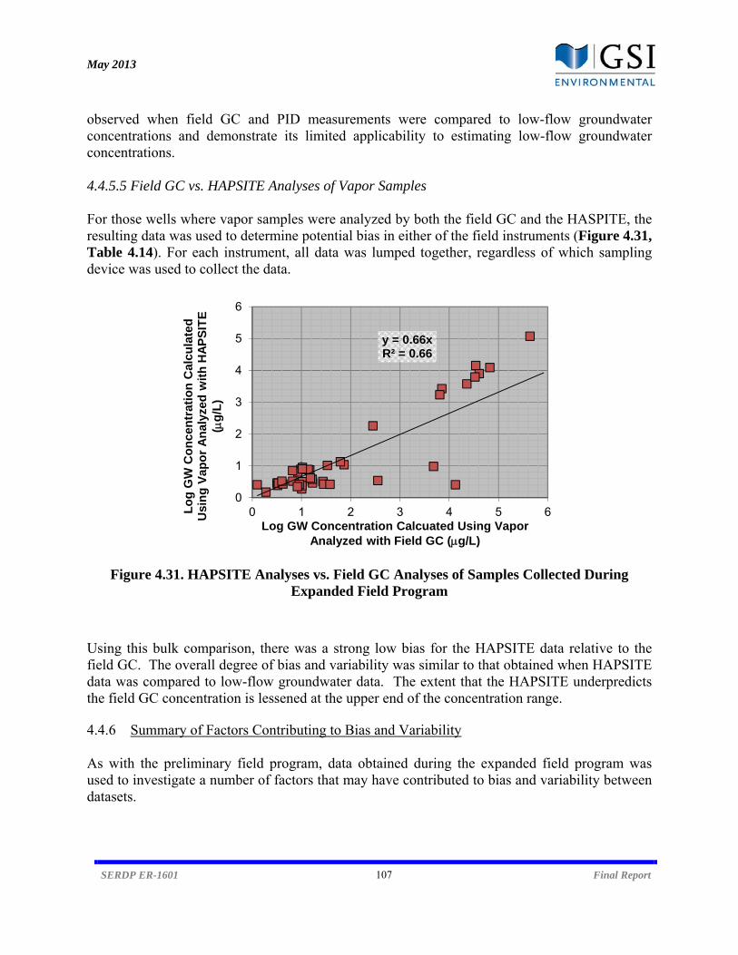
May 2013
SERDP ER-1601 107 Final Report
observed when field GC and PID measurements were compared to low-flow groundwater concentrations and demonstrate its limited applicability to estimating low-flow groundwater concentrations. 4.4.5.5 Field GC vs. HAPSITE Analyses of Vapor Samples For those wells where vapor samples were analyzed by both the field GC and the HASPITE, the resulting data was used to determine potential bias in either of the field instruments (Figure 4.31, Table 4.14). For each instrument, all data was lumped together, regardless of which sampling device was used to collect the data.
Figure 4.31. HAPSITE Analyses vs. Field GC Analyses of Samples Collected During
Expanded Field Program Using this bulk comparison, there was a strong low bias for the HAPSITE data relative to the field GC. The overall degree of bias and variability was similar to that obtained when HAPSITE data was compared to low-flow groundwater data. The extent that the HAPSITE underpredicts the field GC concentration is lessened at the upper end of the concentration range. 4.4.6 Summary of Factors Contributing to Bias and Variability As with the preliminary field program, data obtained during the expanded field program was used to investigate a number of factors that may have contributed to bias and variability between datasets.
y = 0.66xR² = 0.66
0
1
2
3
4
5
6
0 1 2 3 4 5 6Lo
g G
W C
on
cen
trat
ion
Cal
cula
ted
U
sin
g V
apo
r A
nal
yzed
wit
h H
AP
SIT
E
(g
/L)
Log GW Concentration Calcuated Using Vapor Analyzed with Field GC (g/L)
May 2013
SERDP ER-1601 108 Final Report
4.4.6.1 Factors Associated with Sampling and Analysis
Sampling Date: This portion of field testing was completed in April-May 2011, and the data suggested that concentrations within the monitoring wells were generally less vertically stratified than what was observed during the preliminary phase of field testing in January-February 2010. This assumption is based on the similarity between data obtained with a depth-discrete sampler (short PVD) versus data obtained with longer samplers (GSI and Haas balloon PVDs). The prevalence of mixed water columns within the wells is consistent with thermal gradients that would be expected during early spring period in this setting (see Figure 4.5). Consequently, it is unlikely that vertical stratification was a major contributor to variability in this set of field data due to the selected sampling date.
Sample Location: All samples were collected from the middle (or near the middle) of the screened interval during this phase of field testing. Therefore, no additional evaluation of this factor was attempted.
Sample Collection Method: The data quality obtained by the three different passive samplers was very similar, indicating that there was no benefit to be gained from the longer samplers. The short PVD is easier to fabricate and less prone to failure, such that its strong performance during this field program validates its overall utility. However, the ability to correlate vapor samples from the short PVD samplers to groundwater concentration was likely enhanced by temperature gradients that favored mixing within the monitoring wells. If the program were completed during a period with less favorable mixing conditions, the longer PVD samplers may have performed better relative to the short PVD sampler. The field equilibration method continued to exhibit the highest correlation of any of the vapor-based methods for estimating groundwater concentrations.
Vapor Analysis Method: The field GC exhibited the best performance of the three instruments testing during this program. The PID continued to be relatively ineffective in predicting groundwater concentrations, introducing high variability and negative bias. Dilutions were used to minimize detector overload, but variability was still considerable at lower-end concentration range. Some improvement was noted when single constituents were modeled, indicating that the instrument has higher utility in wells dominated by one constituent. The HAPSITE also suffered from high variability and consistently underpredicted concentrations. This may have been a function of the delay between sample collection and sample analysis. The instrument’s low detection limit means it is not prone to false negatives, but given the extent of variability, it appears that it is best suited for screening purposes.
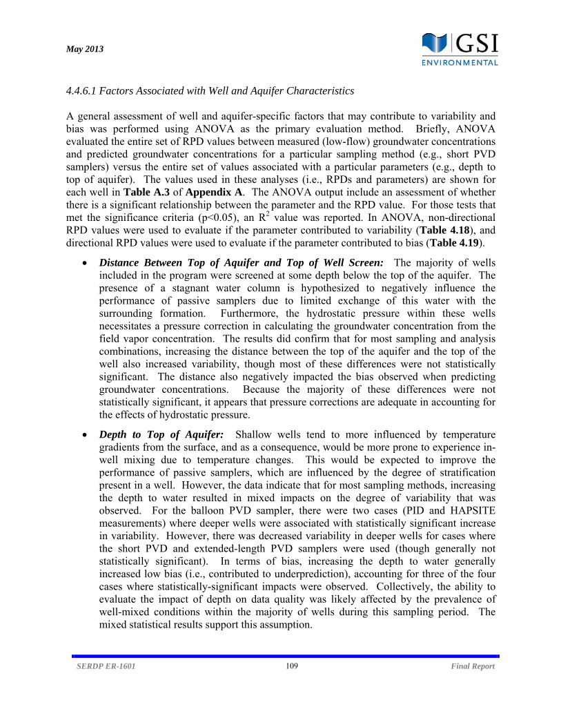
May 2013
SERDP ER-1601 109 Final Report
4.4.6.1 Factors Associated with Well and Aquifer Characteristics
A general assessment of well and aquifer-specific factors that may contribute to variability and bias was performed using ANOVA as the primary evaluation method. Briefly, ANOVA evaluated the entire set of RPD values between measured (low-flow) groundwater concentrations and predicted groundwater concentrations for a particular sampling method (e.g., short PVD samplers) versus the entire set of values associated with a particular parameters (e.g., depth to top of aquifer). The values used in these analyses (i.e., RPDs and parameters) are shown for each well in Table A.3 of Appendix A. The ANOVA output include an assessment of whether there is a significant relationship between the parameter and the RPD value. For those tests that met the significance criteria (p<0.05), an R2 value was reported. In ANOVA, non-directional RPD values were used to evaluate if the parameter contributed to variability (Table 4.18), and directional RPD values were used to evaluate if the parameter contributed to bias (Table 4.19).
Distance Between Top of Aquifer and Top of Well Screen: The majority of wells included in the program were screened at some depth below the top of the aquifer. The presence of a stagnant water column is hypothesized to negatively influence the performance of passive samplers due to limited exchange of this water with the surrounding formation. Furthermore, the hydrostatic pressure within these wells necessitates a pressure correction in calculating the groundwater concentration from the field vapor concentration. The results did confirm that for most sampling and analysis combinations, increasing the distance between the top of the aquifer and the top of the well also increased variability, though most of these differences were not statistically significant. The distance also negatively impacted the bias observed when predicting groundwater concentrations. Because the majority of these differences were not statistically significant, it appears that pressure corrections are adequate in accounting for the effects of hydrostatic pressure.
Depth to Top of Aquifer: Shallow wells tend to more influenced by temperature gradients from the surface, and as a consequence, would be more prone to experience in-well mixing due to temperature changes. This would be expected to improve the performance of passive samplers, which are influenced by the degree of stratification present in a well. However, the data indicate that for most sampling methods, increasing the depth to water resulted in mixed impacts on the degree of variability that was observed. For the balloon PVD sampler, there were two cases (PID and HAPSITE measurements) where deeper wells were associated with statistically significant increase in variability. However, there was decreased variability in deeper wells for cases where the short PVD and extended-length PVD samplers were used (though generally not statistically significant). In terms of bias, increasing the depth to water generally increased low bias (i.e., contributed to underprediction), accounting for three of the four cases where statistically-significant impacts were observed. Collectively, the ability to evaluate the impact of depth on data quality was likely affected by the prevalence of well-mixed conditions within the majority of wells during this sampling period. The mixed statistical results support this assumption.
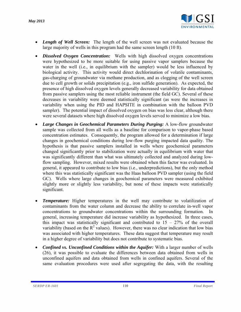
May 2013
SERDP ER-1601 110 Final Report
Length of Well Screen: The length of the well screen was not evaluated because the large majority of wells in this program had the same screen length (10 ft).
Dissolved Oxygen Concentration: Wells with high dissolved oxygen concentrations were hypothesized to be more suitable for using passive vapor samplers because the water in the well (i.e., in equilibrium with the sampler) would be less influenced by biological activity. This activity would direct dechlorination of volatile contaminants, gas-charging of groundwater via methane production, and as clogging of the well screen due to cell growth or solids precipitation (e.g., iron sulfide generation). As expected, the presence of high dissolved oxygen levels generally decreased variability for data obtained from passive samplers using the most reliable instrument (the field GC). Several of these decreases in variability were deemed statistically significant (as were the increases in variability when using the PID and HAPSITE in combination with the balloon PVD sampler). The potential impact of dissolved oxygen on bias was less clear, although there were several datasets where high dissolved oxygen levels served to minimize a low bias.
Large Changes in Geochemical Parameters During Purging: A low-flow groundwater sample was collected from all wells as a baseline for comparison to vapor-phase based concentration estimates. Consequently, the program allowed for a determination if large changes in geochemical conditions during low-flow purging impacted data quality. The hypothesis is that passive samplers installed in wells where geochemical parameters changed significantly prior to stabilization were actually in equilibrium with water that was significantly different than what was ultimately collected and analyzed during low-flow sampling. However, mixed results were obtained when this factor was evaluated. In general, it appeared to contribute to low bias (i.e., underpredictions), but the only method where this was statistically significant was the Haas balloon PVD sampler (using the field GC). Wells where large changes in geochemical parameters were measured exhibited slightly more or slightly less variability, but none of these impacts were statistically significant.
Temperature: Higher temperatures in the well may contribute to volatilization of contaminants from the water column and decrease the ability to correlate in-well vapor concentrations to groundwater concentrations within the surrounding formation. In general, increasing temperature did increase variability as hypothesized. In three cases, this impact was statistically significant and contributed to 15 – 27% of the overall variability (based on the R2 values). However, there was no clear indication that low bias was associated with higher temperatures. These data suggest that temperature may result in a higher degree of variability but does not contribute to systematic bias.
Confined vs. Unconfined Conditions within the Aquifer: With a larger number of wells (26), it was possible to evaluate the differences between data obtained from wells in unconfined aquifers and data obtained from wells in confined aquifers. Several of the same evaluation procedures were used after segregating the data, with the resulting
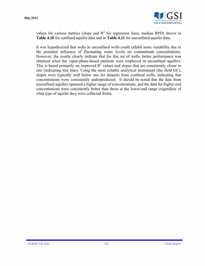
May 2013
SERDP ER-1601 111 Final Report
values for various metrics (slope and R2 for regression lines, median RPD) shown in Table 4.20 for confined aquifer data and in Table 4.21 for unconfined aquifer data. It was hypothesized that wells in unconfined wells could exhibit more variability due to the potential influence of fluctuating water levels on contaminant concentrations. However, the results clearly indicate that for this set of wells, better performance was obtained when the vapor-phase-based methods were employed in unconfined aquifers. This is based primarily on improved R2 values and slopes that are consistently closer to one (indicating less bias). Using the most reliable analytical instrument (the field GC), slopes were typically well below one for datasets from confined wells, indicating that concentrations were consistently underpredicted. It should be noted that the data from unconfined aquifers spanned a higher range of concentrations, and the data for higher-end concentrations were consistently better than those at the lower-end range (regardless of what type of aquifer they were collected from).
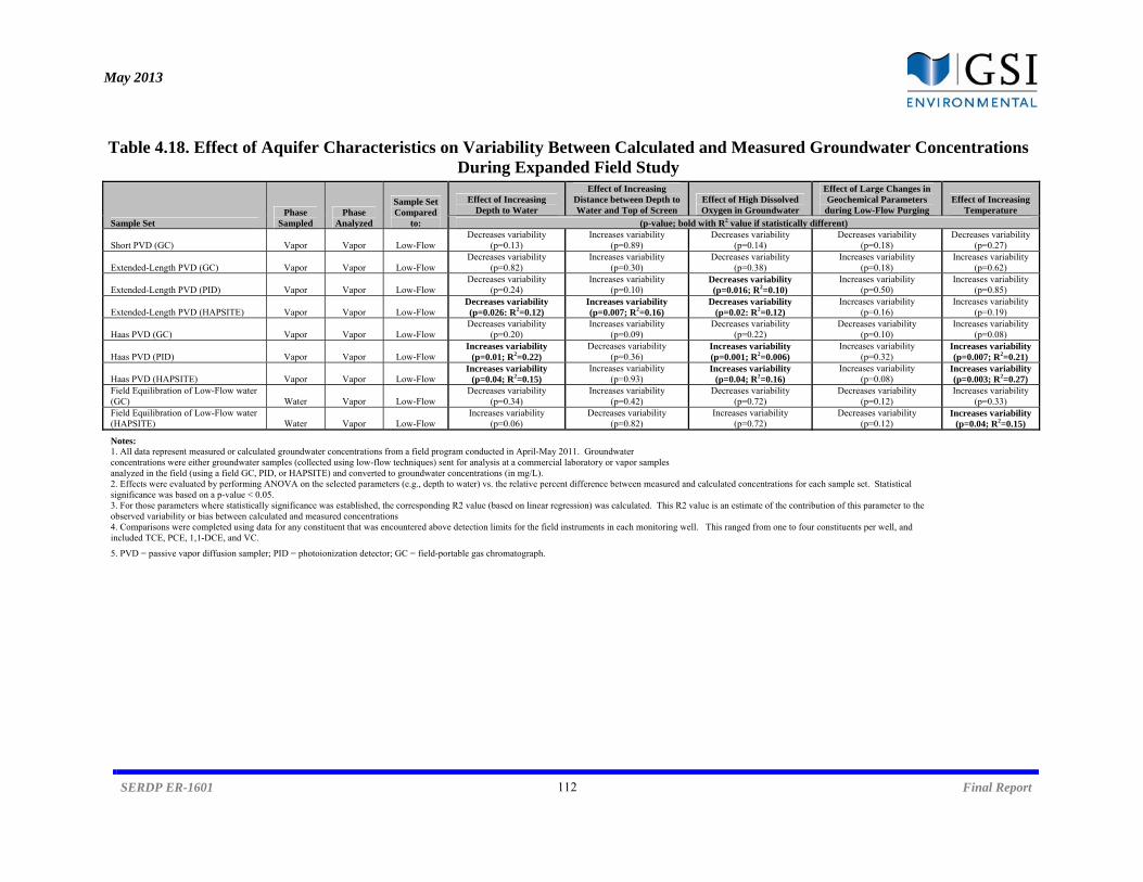
May 2013
SERDP ER-1601 112 Final Report
Table 4.18. Effect of Aquifer Characteristics on Variability Between Calculated and Measured Groundwater Concentrations During Expanded Field Study
Sample Set Phase
Sampled Phase
Analyzed
Sample Set Compared
to:
Effect of Increasing Depth to Water
Effect of Increasing Distance between Depth to Water and Top of Screen
Effect of High Dissolved Oxygen in Groundwater
Effect of Large Changes in Geochemical Parameters during Low-Flow Purging
Effect of Increasing Temperature
(p-value; bold with R2 value if statistically different)
Short PVD (GC) Vapor Vapor Low-Flow Decreases variability
(p=0.13) Increases variability
(p=0.89) Decreases variability
(p=0.14) Decreases variability
(p=0.18) Decreases variability
(p=0.27)
Extended-Length PVD (GC) Vapor Vapor Low-Flow Decreases variability
(p=0.82) Increases variability
(p=0.30) Decreases variability
(p=0.38) Increases variability
(p=0.18) Increases variability
(p=0.62)
Extended-Length PVD (PID) Vapor Vapor Low-Flow Decreases variability
(p=0.24) Increases variability
(p=0.10) Decreases variability (p=0.016; R2=0.10)
Increases variability (p=0.50)
Increases variability (p=0.85)
Extended-Length PVD (HAPSITE) Vapor Vapor Low-Flow Decreases variability (p=0.026: R2=0.12)
Increases variability (p=0.007; R2=0.16)
Decreases variability (p=0.02: R2=0.12)
Increases variability (p=0.16)
Increases variability (p=0.19)
Haas PVD (GC) Vapor Vapor Low-Flow Decreases variability
(p=0.20) Increases variability
(p=0.09) Decreases variability
(p=0.22) Decreases variability
(p=0.10) Increases variability
(p=0.08)
Haas PVD (PID) Vapor Vapor Low-Flow Increases variability
(p=0.01; R2=0.22) Decreases variability
(p=0.36) Increases variability (p=0.001; R2=0.006)
Increases variability (p=0.32)
Increases variability(p=0.007; R2=0.21)
Haas PVD (HAPSITE) Vapor Vapor Low-Flow Increases variability
(p=0.04; R2=0.15) Increases variability
(p=0.93) Increases variability
(p=0.04; R2=0.16) Increases variability
(p=0.08) Increases variability(p=0.003; R2=0.27)
Field Equilibration of Low-Flow water (GC) Water Vapor Low-Flow
Decreases variability (p=0.34)
Increases variability (p=0.42)
Decreases variability (p=0.72)
Decreases variability (p=0.12)
Increases variability (p=0.33)
Field Equilibration of Low-Flow water (HAPSITE) Water Vapor Low-Flow
Increases variability (p=0.06)
Decreases variability (p=0.82)
Increases variability (p=0.72)
Decreases variability (p=0.12)
Increases variability(p=0.04; R2=0.15)
Notes:
1. All data represent measured or calculated groundwater concentrations from a field program conducted in April-May 2011. Groundwater concentrations were either groundwater samples (collected using low-flow techniques) sent for analysis at a commercial laboratory or vapor samples analyzed in the field (using a field GC, PID, or HAPSITE) and converted to groundwater concentrations (in mg/L).
2. Effects were evaluated by performing ANOVA on the selected parameters (e.g., depth to water) vs. the relative percent difference between measured and calculated concentrations for each sample set. Statistical significance was based on a p-value < 0.05. 3. For those parameters where statistically significance was established, the corresponding R2 value (based on linear regression) was calculated. This R2 value is an estimate of the contribution of this parameter to the observed variability or bias between calculated and measured concentrations
4. Comparisons were completed using data for any constituent that was encountered above detection limits for the field instruments in each monitoring well. This ranged from one to four constituents per well, and included TCE, PCE, 1,1-DCE, and VC.
5. PVD = passive vapor diffusion sampler; PID = photoionization detector; GC = field-portable gas chromatograph.
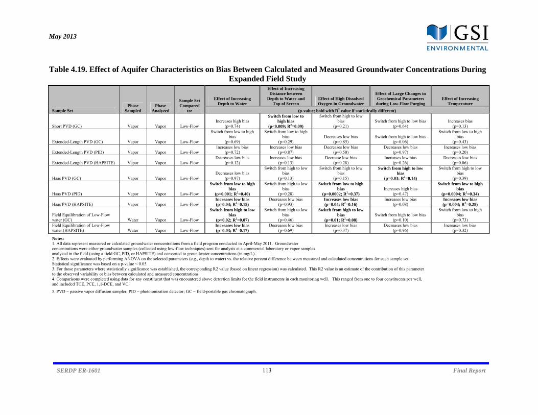
May 2013
SERDP ER-1601 113 Final Report
Table 4.19. Effect of Aquifer Characteristics on Bias Between Calculated and Measured Groundwater Concentrations During Expanded Field Study
Sample Set Phase
Sampled Phase
Analyzed
Sample Set Compared
to:
Effect of Increasing Depth to Water
Effect of Increasing Distance between
Depth to Water and Top of Screen
Effect of High Dissolved Oxygen in Groundwater
Effect of Large Changes in Geochemical Parameters during Low-Flow Purging
Effect of Increasing Temperature
(p-value; bold with R2 value if statistically different)
Short PVD (GC) Vapor Vapor Low-Flow Increases high bias
(p=0.74)
Switch from low to high bias
(p<0.009; R2=0.09)
Switch from high to low bias
(p=0.21) Switch from high to low bias
(p=0.64) Increases bias
(p=0.13)
Extended-Length PVD (GC) Vapor Vapor Low-Flow
Switch from low to high bias
(p=0.69)
Switch from low to high bias
(p=0.29) Decreases low bias
(p=0.85) Switch from high to low bias
(p=0.06)
Switch from low to high bias
(p=0.43)
Extended-Length PVD (PID) Vapor Vapor Low-Flow Increases low bias
(p=0.72) Increases low bias
(p=0.87) Decreases low bias
(p=0.50) Decreases low bias
(p=0.97) Increases low bias
(p=0.20)
Extended-Length PVD (HAPSITE) Vapor Vapor Low-Flow Decreases low bias
(p=0.12) Increases low bias
(p=0.13) Decrease low bias
(p=0.28) Increases low bias
(p=0.26) Decreases low bias
(p=0.06)
Haas PVD (GC) Vapor Vapor Low-Flow Decreases low bias
(p=0.97)
Switch from high to low bias
(p=0.13)
Switch from high to low bias
(p=0.15)
Switch from high to low bias
(p=0.03: R2=0.14)
Switch from high to low bias
(p=0.39)
Haas PVD (PID) Vapor Vapor Low-Flow
Switch from low to high bias
(p<0.001; R2=0.40)
Switch from high to low bias
(p=0.28)
Switch from low to high bias
(p=0.0002; R2=0.37) Increases high bias
(p=0.47)
Switch from low to high bias
(p=0.0004; R2=0.34)
Haas PVD (HAPSITE) Vapor Vapor Low-Flow Increases low bias (p=0.04; R2=0.15)
Decreases low bias (p=0.93)
Increases low bias (p=0.04; R2=0.16)
Increases low bias (p=0.08)
Increases low bias (p=0.004; R2=0.28)
Field Equilibration of Low-Flow water (GC) Water Vapor Low-Flow
Switch from high to low bias
(p=0.02; R2=0.07)
Switch from high to low bias
(p=0.46)
Switch from high to low bias
(p=0.01; R2=0.08) Switch from high to low bias
(p=0.10)
Switch from low to high bias
(p=0.73) Field Equilibration of Low-Flow water (HAPSITE) Water Vapor Low-Flow
Increases low bias (p=0.03; R2=0.17)
Decreases low bias (p=0.69)
Increases low bias (p=0.37)
Decreases low bias (p=0.96)
Increases low bias (p=0.32)
Notes:
1. All data represent measured or calculated groundwater concentrations from a field program conducted in April-May 2011. Groundwater concentrations were either groundwater samples (collected using low-flow techniques) sent for analysis at a commercial laboratory or vapor samples analyzed in the field (using a field GC, PID, or HAPSITE) and converted to groundwater concentrations (in mg/L).
2. Effects were evaluated by performing ANOVA on the selected parameters (e.g., depth to water) vs. the relative percent difference between measured and calculated concentrations for each sample set. Statistical significance was based on a p-value < 0.05. 3. For those parameters where statistically significance was established, the corresponding R2 value (based on linear regression) was calculated. This R2 value is an estimate of the contribution of this parameter to the observed variability or bias between calculated and measured concentrations.
4. Comparisons were completed using data for any constituent that was encountered above detection limits for the field instruments in each monitoring well. This ranged from one to four constituents per well, and included TCE, PCE, 1,1-DCE, and VC.
5. PVD = passive vapor diffusion sampler; PID = photoionization detector; GC = field-portable gas chromatograph.
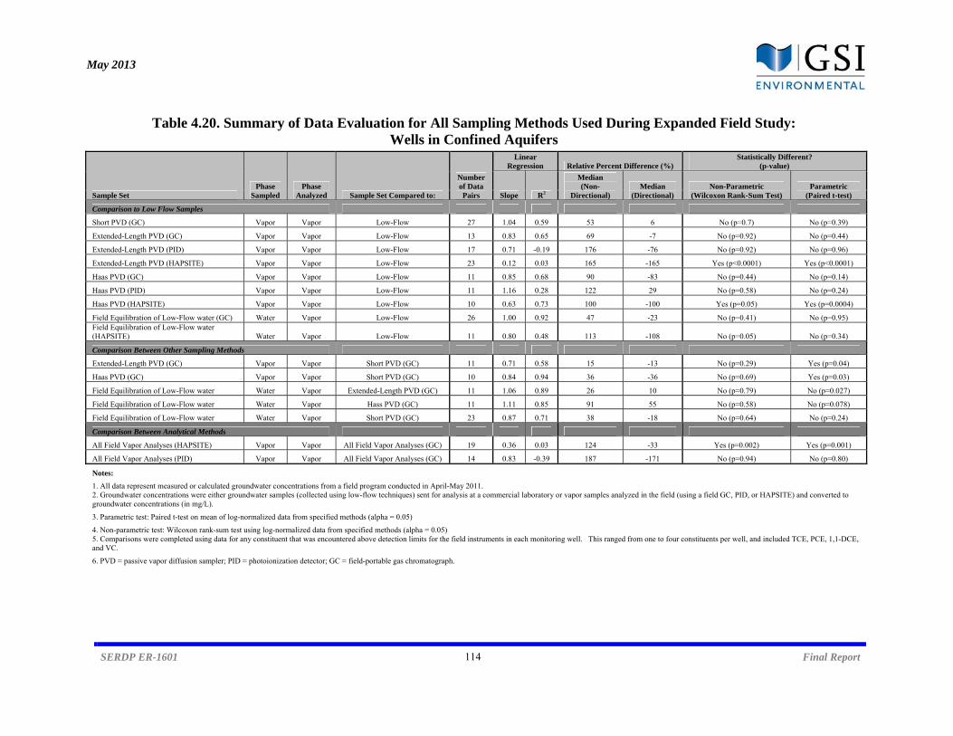
May 2013
SERDP ER-1601 114 Final Report
Table 4.20. Summary of Data Evaluation for All Sampling Methods Used During Expanded Field Study: Wells in Confined Aquifers
Sample Set Phase
Sampled Phase
Analyzed Sample Set Compared to:
Number of Data Pairs
Linear Regression Relative Percent Difference (%)
Statistically Different? (p-value)
Slope R2
Median (Non-
Directional) Median
(Directional) Non-Parametric
(Wilcoxon Rank-Sum Test) Parametric
(Paired t-test)
Comparison to Low Flow Samples
Short PVD (GC) Vapor Vapor Low-Flow 27 1.04 0.59 53 6 No (p=0.7) No (p=0.39)
Extended-Length PVD (GC) Vapor Vapor Low-Flow 13 0.83 0.65 69 -7 No (p=0.92) No (p=0.44)
Extended-Length PVD (PID) Vapor Vapor Low-Flow 17 0.71 -0.19 176 -76 No (p=0.92) No (p=0.96)
Extended-Length PVD (HAPSITE) Vapor Vapor Low-Flow 23 0.12 0.03 165 -165 Yes (p<0.0001) Yes (p<0.0001)
Haas PVD (GC) Vapor Vapor Low-Flow 11 0.85 0.68 90 -83 No (p=0.44) No (p=0.14)
Haas PVD (PID) Vapor Vapor Low-Flow 11 1.16 0.28 122 29 No (p=0.58) No (p=0.24)
Haas PVD (HAPSITE) Vapor Vapor Low-Flow 10 0.63 0.73 100 -100 Yes (p=0.05) Yes (p=0.0004)
Field Equilibration of Low-Flow water (GC) Water Vapor Low-Flow 26 1.00 0.92 47 -23 No (p=0.41) No (p=0.95) Field Equilibration of Low-Flow water (HAPSITE) Water Vapor Low-Flow 11 0.80 0.48 113 -108 No (p=0.05) No (p=0.34)
Comparison Between Other Sampling Methods
Extended-Length PVD (GC) Vapor Vapor Short PVD (GC) 11 0.71 0.58 15 -13 No (p=0.29) Yes (p=0.04)
Haas PVD (GC) Vapor Vapor Short PVD (GC) 10 0.84 0.94 36 -36 No (p=0.69) Yes (p=0.03)
Field Equilibration of Low-Flow water Water Vapor Extended-Length PVD (GC) 11 1.06 0.89 26 10 No (p=0.79) No (p=0.027)
Field Equilibration of Low-Flow water Water Vapor Hass PVD (GC) 11 1.11 0.85 91 55 No (p=0.58) No (p=0.078)
Field Equilibration of Low-Flow water Water Vapor Short PVD (GC) 23 0.87 0.71 38 -18 No (p=0.64) No (p=0.24)
Comparison Between Analytical Methods
All Field Vapor Analyses (HAPSITE) Vapor Vapor All Field Vapor Analyses (GC) 19 0.36 0.03 124 -33 Yes (p=0.002) Yes (p=0.001)
All Field Vapor Analyses (PID) Vapor Vapor All Field Vapor Analyses (GC) 14 0.83 -0.39 187 -171 No (p=0.94) No (p=0.80)
Notes: 1. All data represent measured or calculated groundwater concentrations from a field program conducted in April-May 2011. 2. Groundwater concentrations were either groundwater samples (collected using low-flow techniques) sent for analysis at a commercial laboratory or vapor samples analyzed in the field (using a field GC, PID, or HAPSITE) and converted to groundwater concentrations (in mg/L).
3. Parametric test: Paired t-test on mean of log-normalized data from specified methods (alpha = 0.05)
4. Non-parametric test: Wilcoxon rank-sum test using log-normalized data from specified methods (alpha = 0.05) 5. Comparisons were completed using data for any constituent that was encountered above detection limits for the field instruments in each monitoring well. This ranged from one to four constituents per well, and included TCE, PCE, 1,1-DCE, and VC.
6. PVD = passive vapor diffusion sampler; PID = photoionization detector; GC = field-portable gas chromatograph.

May 2013
SERDP ER-1601 115 Final Report
Table 4.21. Summary of Data Evaluation for All Sampling Methods Used During Expanded Field Study: Wells in Unconfined Aquifers
Sample Set Phase
Sampled Phase
Analyzed Sample Set Compared to:
Number of Data Pairs
Linear Regression Relative Percent Difference (%) Statistically Different?
(p-value)
Slope R2 Median
(Non-Directional) Median
(Directional)
Non-Parametric (Wilcoxon Rank-
Sum Test) Parametric
(Paired t-test)
Comparison to Low Flow Samples
Short PVD (GC) Vapor Vapor Low-Flow 47 1.06 0.94 78 57 No (p=0.41 Yes (p=0.007)
Extended-Length PVD (GC) Vapor Vapor Low-Flow 22 1.05 0.97 89 42 No (p=0.83) No (p=0.18)
Extended-Length PVD (PID) Vapor Vapor Low-Flow 38 0.84 0.90 96 -96 No (p=0.34) Yes (p<0.0001)
Extended-Length PVD (HAPSITE) Vapor Vapor Low-Flow 19 0.81 0.87 78 -78 Yes (p=0.02) Yes (p<0.0001)
Haas PVD (GC) Vapor Vapor Low-Flow 24 1.05 0.94 76 59 No (p=0.88) No (p=0.31)
Haas PVD (PID) Vapor Vapor Low-Flow 22 0.95 -2.8 133 -1 No (p=0.45) No (p=0.08)
Haas PVD (HAPSITE) Vapor Vapor Low-Flow 18 0.87 0.87 91 -91 Yes (p=0.008) Yes (p<0.0001)
Field Equilibration of Low-Flow water (GC) Water Vapor Low-Flow 48 1.02 0.98 34 5 No (p=0.70) No (p=0.98) Field Equilibration of Low-Flow water (HAPSITE) Water Vapor Low-Flow 18 0.72 0.77 165 -165 Yes (p=0.0003) Yes (p<0.0001)
Comparison Between Other Sampling Methods
Extended-Length PVD (GC) Vapor Vapor Short PVD (GC) 20 0.98 0.97 86 -46 No (p=0.78) No (p=0.26)
Haas PVD (GC) Vapor Vapor Short PVD (GC) 22 0.94 0.96 61 -24 No (p=0.47) Yes (p=0.012)
Field Equilibration of Low-Flow water Water Vapor Extended-Length PVD (GC) 21 0.94 0.95 65 -58 No (p=0.76) No (p=0.12)
Field Equilibration of Low-Flow water Water Vapor Hass PVD (GC) 24 0.97 0.95 40 -5 No (p=0.80) No (p=0.54)
Field Equilibration of Low-Flow water Water Vapor Short PVD (GC) 45 0.94 0.97 46 -39 No (p=0.24) Yes (p<0.0001)
Comparison Between Analytical Methods
All Field Vapor Analyses (HAPSITE) Vapor Vapor All Field Vapor Analyses (GC) 27 0.82 0.93 115 -115 Yes (p<0.0001) Yes (p<0.0001)
All Field Vapor Analyses (PID) Vapor Vapor All Field Vapor Analyses (GC) 30 0.81 0.54 173 -107 No (p=0.59) No (p=0.47)
Notes: 1. All data represent measured or calculated groundwater concentrations from a field program conducted in April-May 2011. 2. Groundwater concentrations were either groundwater samples (collected using low-flow techniques) sent for analysis at a commercial laboratory or vapor samples analyzed in the field (using a field GC, PID, or HAPSITE) and converted to groundwater concentrations (in mg/L).
3. Parametric test: Paired t-test on mean of log-normalized data from specified methods (alpha = 0.05)
4. Non-parametric test: Wilcoxon rank-sum test using log-normalized data from specified methods (alpha = 0.05) 5. Comparisons were completed using data for any constituent that was encountered above detection limits for the field instruments in each monitoring well. This ranged from one to four constituents per well, and included TCE, PCE, 1,1-DCE, and VC.
6. PVD = passive vapor diffusion sampler; PID = photoionization detector; GC = field-portable gas chromatograph.

May 2013
SERDP ER-1601 116 Final Report
4.5 Supplemental Field Program The supplemental field program was completed during 15 separate events between September 2011 and August 2012 in the same set of 8 wells. The sampling methods that had been validated during the preliminary field study were included in this phase (see Section 4.3), specifically the “short” PVD samplers (i.e., gas-filled 40-mL vials wrapped in LDPE and submerged below the water level) and the field equilibration method (i.e., 20 mL of groundwater transferred to sealed 40-mL vials, with the headspace analyzed in the field following 40 to 60 minutes of equilibration time). Low-flow groundwater samples were again used as the baseline comparison for groundwater concentration estimated using the vapor-phase method. The primary difference is that several variations on groundwater sampling were also completed during at least three of the fifteen events as part of the concurrent program for SERDP ER-1705. These variations included no-purge groundwater sampling, low-flow groundwater sampling with purging to parameter stability, low-flow groundwater sampling with purging of a fixed volume (24 L per well), low-flow groundwater sampling following in-well mixing, and groundwater sampling using the Snap samplers (without purging). The field GC was the only instrument used during on-site vapor analysis. The monitoring events were scheduled for a period that spanned nearly an entire calendar year, such that monitoring occurred during both periods that favored thermally mixed conditions (late spring) as well as periods that favored thermal stratification (late winter) based on the results of the temperature study (see Section 4.2). 4.5.1 Well Characteristics and Sampling Data Table A.5 (Appendix A) summarizes pertinent characteristics for the wells included in the field program. Monitoring was completed at 8 wells installed at the same site within an unconfined aquifer. Seven of the eight were 2-in diameter wells, with one 4-in diameter well. The total depth of these wells ranged from approximately 18 ft to 33 ft, with a depth to water that generally ranged between 4 and 13 feet. The majority of wells (7 of 8) had screens that were 10 ft in length. In 21 of the 24 instances when the depth to water was measured (encompassing both sampling events), the water level was higher than the top of the screen interval (well MW-8 was the consistent exception). Owing to the proximity of the site to a large bay, groundwater samples consistently exhibited high salinity during field measurements (electrical conductivity consistently between 10 and 40 mS/cm). The groundwater was also moderately reducing (low dissolved oxygen and negative oxidation-reduction potential) and acidic (pH frequently below 6). On-site pumping is believed to result in a relatively consistent hydraulic gradient, such that water from the bay is regularly pulled into the groundwater-bearing unit. During the field program, groundwater and vapor samples were collected from each monitoring well using a series of different methods and analyzed either in the field or following shipment to a commercial laboratory. Table 4.22 summarizes the total number of samples collected using each of these methods.

May 2013
SERDP ER-1601 117 Final Report
Table 4.22. Datasets Generated During Supplemental Field Program: Joint Program with
SERDP ER-1705 Sample Method No. of Datasets
Obtained1 No. of Datapoints
Obtained Short PVD2 334 264 Field Equilibration – No purge2 95 72 Field Equilibration – No purge with in-well mixing2 3 24 Field Equilibration – Following purge to parameter stability2 4 32 Field Equilibration – Following purge constant volume2 3 24 Low-Flow – No purge3 96 72 Low-Flow – No purge with in-well mixing3 3 24 Low-Flow – Purge to parameter stability3 5 40 Low-Flow- Purge constant volume3 3 24 No purge Snap groundwater sampler3 3 24 Notes: (1) Each dataset consists of VOC concentrations from the same 8 wells. See Table 3.8 for schedule; (2) Method
consists of groundwater concentration obtained from field vapor-phase analysis completed specifically for SERDP ER-1601; (3) Method consists of groundwater concentration obtained from laboratory water-phase analysis completed for SERDP ER-1705; (4) 11 datasets obtained for each depth at which a short PVD sampler was installed (top of screen, middle of screen, bottom of screen); (5) Includes field equilibration samples collected during no-purge groundwater sampling events (i.e., Weeks 7, 22, and 37 in Table 3.8) as well as field equilibration samples collected during the initial stages of purging (“pre-purge”) during low-flow groundwater sampling events; (6) Includes “pre-purge” groundwater samples collected during the initial stages of purging during low-flow groundwater sampling events.
A total of 600 vapor and groundwater sample analyses were performed as part of the field program, not including replicates. Vapor concentrations of all detected constituents were converted to groundwater concentrations using the procedure outlined in Section 3.5. The eight wells in the monitoring program had detectable concentrations of multiple constituents, including VC, 1,1-DCE, benzene, chlorobenzene, and ethyl benzene. To simplify comparisons between the vapor-based methods and conventional groundwater sampling and analysis (and in particular the variability associated with each method), only the vapor analytical results for VC were used. The resulting groundwater concentration data (both measured concentrations in groundwater samples and calculated concentrations based on conversion of the vapor data) are summarized in Table A.6 in Appendix A. The raw vapor-phase concentration data are included in Table A.7 of Appendix A. As with the concentration data from the previous field programs, the data from the supplemental field program was log-transformed to improve the normality of the data and the power of the statistical methods used to evaluate the data. Log transformation did not result in normally distributed data based on the protocol for the Anderson Darling test for normality (p < 0.05) except for select datasets. However, in all cases, log transformation improved the normality relative to non-transformed data (i.e., lowered the value of the test statistic). Therefore, log-transformed data were used in further evaluation of the data.
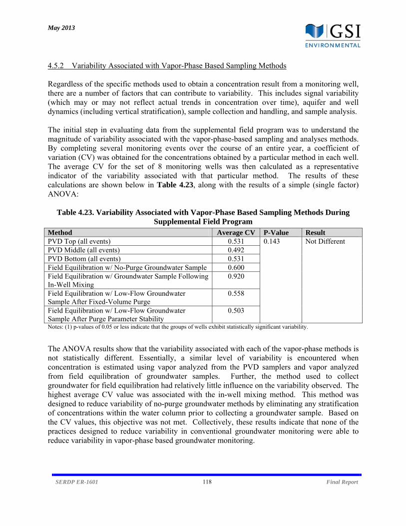
May 2013
SERDP ER-1601 118 Final Report
4.5.2 Variability Associated with Vapor-Phase Based Sampling Methods Regardless of the specific methods used to obtain a concentration result from a monitoring well, there are a number of factors that can contribute to variability. This includes signal variability (which may or may not reflect actual trends in concentration over time), aquifer and well dynamics (including vertical stratification), sample collection and handling, and sample analysis. The initial step in evaluating data from the supplemental field program was to understand the magnitude of variability associated with the vapor-phase-based sampling and analyses methods. By completing several monitoring events over the course of an entire year, a coefficient of variation (CV) was obtained for the concentrations obtained by a particular method in each well. The average CV for the set of 8 monitoring wells was then calculated as a representative indicator of the variability associated with that particular method. The results of these calculations are shown below in Table 4.23, along with the results of a simple (single factor) ANOVA:
Table 4.23. Variability Associated with Vapor-Phase Based Sampling Methods During Supplemental Field Program
Method Average CV P-Value Result PVD Top (all events) 0.531 0.143 Not Different PVD Middle (all events) 0.492 PVD Bottom (all events) 0.531 Field Equilibration w/ No-Purge Groundwater Sample 0.600 Field Equilibration w/ Groundwater Sample Following In-Well Mixing
0.920
Field Equilibration w/ Low-Flow Groundwater Sample After Fixed-Volume Purge
0.558
Field Equilibration w/ Low-Flow Groundwater Sample After Purge Parameter Stability
0.503
Notes: (1) p-values of 0.05 or less indicate that the groups of wells exhibit statistically significant variability.
The ANOVA results show that the variability associated with each of the vapor-phase methods is not statistically different. Essentially, a similar level of variability is encountered when concentration is estimated using vapor analyzed from the PVD samplers and vapor analyzed from field equilibration of groundwater samples. Further, the method used to collect groundwater for field equilibration had relatively little influence on the variability observed. The highest average CV value was associated with the in-well mixing method. This method was designed to reduce variability of no-purge groundwater methods by eliminating any stratification of concentrations within the water column prior to collecting a groundwater sample. Based on the CV values, this objective was not met. Collectively, these results indicate that none of the practices designed to reduce variability in conventional groundwater monitoring were able to reduce variability in vapor-phase based groundwater monitoring.
May 2013
SERDP ER-1601 119 Final Report
Additional ANOVA comparisons between smaller groups of data are presented in Table A.8 of Appendix A. In all cases, these tests showed that there was no statistical significant difference in the variability associated with any of these vapor-based methods. This includes comparisons when the PVD data from samplers installed at three different depths within the same well are averaged (generating a single CV value). In addition to simple ANOVA, a variety of parametric and non-parametric tests were used to compare the variability associated with the monitoring methods. These tests, which are presented in Table A.9 of Appendix A, take advantage of the fact that these are paired datasets (i.e., most vapor-phase based concentrations were obtained from the same set of wells on the same dates). In general, these tests were unable to demonstrate that there are statistically significant differences in variability associated with any of the vapor-phase based methods. The only two exceptions were associated with the field equilibration method, with data obtained using the in-well mixing approach more variable than data obtained from both the fixed-volume purge and the purge to parameter stability. Previous investigations have demonstrated that the variability associated with vapor analysis are very low (Median RSD < 5% in laboratory validation study. < 8% in preliminary field program, and < 6% in expanded field program). Further, the variability associated with sample collection and handling has been shown by this project and SERDP ER-1705 to be similarly small (RSD values on the order of 5%). Therefore, the majority of variability appears to be associated with well/aquifer factors and changes in the actual groundwater concentration (both time-dependent and time-independent changes). 4.5.3. Variability of Vapor-Phase Based Sampling Methods Relative to Groundwater Sampling
Methods This step in the evaluation was designed to answer two questions: 1) Is the variability associated with vapor-phase monitoring similar to that observed with direct groundwater monitoring methods?; and 2) Are methods designed to influence variability in groundwater sampling have any impact on vapor-phase-based methods? Because groundwater samples were collected and analyzed from the same set of monitoring wells during the same intervals, the program allowed for a direct comparison between the level of variability associated with groundwater sampling and the vapor-phase based methods. In particular, this approach means that the signal variability (associated with natural fluctuations or changes in groundwater concentrations over time) will be the same regardless of the method being employed to obtain the concentration result. Consequently, signal variability is removed as a confounding factor for understanding the relative variability associated with each method. The results of these calculations are shown below in Table 4.24, along with the results of a simple (single factor) ANOVA that considered all datasets. The entire range of data for each method are shown in Figure 4.32 as box plots.

May 2013
SERDP ER-1601 120 Final Report
Table 4.24. Variability Associated with Vapor-Phase Based Sampling Methods Relative to
Groundwater Sampling Methods During Supplemental Field Program Method Average
CV P-Value Result
Vapor-Phase Based
PVD Top (all events) 0.531 0.403 Not Different PVD Middle (all events) 0.492 PVD Bottom (all events) 0.531 Field Equilibration w/ No-Purge Groundwater Sample
0.600
Field Equilibration w/ Groundwater Sample Following In-Well Mixing
0.920
Field Equilibration w/ Low-Flow Groundwater Sample After Fixed-Volume Purge
0.558
Field Equilibration w/ Low-Flow Groundwater Sample After Purge to Parameter Stability
0.503
Groundwater Based
Low-Flow Groundwater Sampler After Purge to Parameter Stability
0.532
Low-Flow Groundwater Sample After Fixed-Volume Purge
0.684
No-Purge Low-Flow Groundwater Sample 0.572 Snap Sampler 0.625 In-Well Mixing Prior to No-Purge Low-Flow Groundwater Sampling
0.533
Notes: (1) P-values of 0.05 or less indicate that the groups of wells exhibit statistically significant variability; (2) Only vinyl chloride data included in calculation of average CV values for groundwater sampling methods.
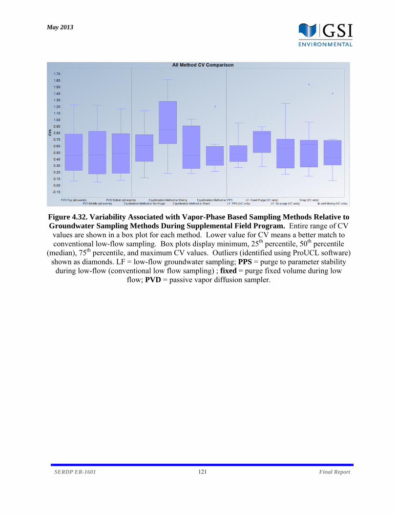
May 2013
SERDP ER-1601 121 Final Report
Figure 4.32. Variability Associated with Vapor-Phase Based Sampling Methods Relative to Groundwater Sampling Methods During Supplemental Field Program. Entire range of CV values are shown in a box plot for each method. Lower value for CV means a better match to conventional low-flow sampling. Box plots display minimum, 25th percentile, 50th percentile
(median), 75th percentile, and maximum CV values. Outliers (identified using ProUCL software) shown as diamonds. LF = low-flow groundwater sampling; PPS = purge to parameter stability
during low-flow (conventional low flow sampling) ; fixed = purge fixed volume during low flow; PVD = passive vapor diffusion sampler.
May 2013
SERDP ER-1601 122 Final Report
The ANOVA results demonstrate that the variability associated with each of the vapor-phase methods is not statistically different than the variability associated with groundwater-based methods. The level of variability was similar regardless of how the groundwater concentration was determined. Collectively, these results indicate that none of the practices designed to reduce variability in conventional groundwater monitoring were very effective at this goal. This finding applies to both vapor-phase based groundwater monitoring data and conventionally-collected (low-flow) groundwater monitoring data. While the vapor-based concentration dataset with the highest variability was associated with in-well mixing, groundwater data obtained after in-well mixing was very similar to the other groundwater datasets. There is no practical explanation for why this occurred since both relied on collecting and analyzing the same groundwater samples. The primary difference is that the vapor analyses for these samples were completed on-site with the field GC (while the groundwater analyses were completed off-site at a commercial lab). Additional ANOVA comparisons between smaller groups of vapor-phase-based and groundwater sampling data are presented in Table A.8 of Appendix A. To simplify the number of analyses, the focus was on comparisons where the PVD data from samplers installed at three different depths within the same well are averaged (generating a single CV value). In all cases, these tests showed that there was no statistical significant difference in the variability associated with any of the methods. 4.5.4 Comparison of Concentrations Obtained using Vapor-Phase Based Sampling Methods vs.
Groundwater Sampling Methods During the supplemental field program, the comparison of concentrations obtained using vapor-phase based methods to conventional groundwater monitoring followed the same methodology used during earlier project-related field programs. Specifically, linear regression, two-sample tests, ANOVA, and relative percent differences were employed in various comparisons. The results of these comparisons are summarized in Table 4.25. All linear regression plots are included in Figure A.4 of Appendix A. Box plots displaying differences in concentration by method are shown in Figure 4.33. A full discussion of each paired comparison is not presented here because the trends were consistent with those in previous phases of field testing. The following findings are highlighted:
The field equilibration method resulted in more accurate matching of groundwater concentrations than the PVD sampler-based method. This is based on uniformly higher R2 values during linear regression and lower median RPD values. Further, there were more instances where the field equilibration method results in concentration datasets that were not statistically significantly different than corresponding direct groundwater measurements. These findings are consistent with earlier field trials where the field equilibration method generated the strongest results, and this consistency is attributable to

May 2013
SERDP ER-1601 123 Final Report
the fact that the same groundwater being analyzed in a commercial lab (as a baseline) is being collected for on-site vapor analyses (following equilibration). This is particularly applicable for comparisons with post-purge groundwater, where the PVD samplers are at a disadvantage because they represent more of a time-weighted average of groundwater from the period when they were deployed. In fact, higher R2 values were achieved for the field equilibration method than for the PVD sampling method when regressions were attempted with the post-purge groundwater.
Of note is that the field equilibration method tended to slightly underpredict the actual groundwater concentration, based on the slopes of the regression lines and the negative RPD values. This directional bias was also observed during the one of the two other field trials (see Section 4.3.3). It is likely due to either incomplete water-vapor equilibration following sample collection or minor volatilization of contaminants from the half-filled equilibration vials in the short period between sample collection and analysis.
For the field equilibration method, there was no clear difference between the correlations obtained with no-purge groundwater datasets versus post-purge groundwater datasets. The latter had a higher overall R2 value (0.97 to 0.99) following linear regression, but similar or higher RPD values (depending on the purging endpoint). Of all the groundwater sampling methods utilized during this study, the data generated following in-well mixing was the least correlated to the data generated during field equilibration. However, the two datasets were not consistently different based on the various two-sample statistical tests that were run.
The PVD samplers still provided reasonable correlations with concentrations determined through direct measurement of groundwater. However, the R2 values obtained during this phase of field testing (range = 0.63 – 0.87) were generally lower than those during earlier phases (average = 0.85). The PVD samplers tended to overpredict the actual groundwater concentration slightly (based on the slope of the regression lines and the positive RPD values), regardless of what method was used to collect the groundwater sample. The bias was large enough to result in concentration datasets that were nearly all statistically significantly different than corresponding direct groundwater measurements. A similar bias towards overprediction was noted in earlier field trials, although not to the extent seen during this phase. The reason for this bias is unknown, but it may be related to deployment conditions that are not properly accounted for during conversion of the vapor-phase concentration to an equivalent groundwater concentration. For example, changes in pressure and/or temperature following retrieval may negatively impact equilibrium partitioning calculations. The influences of pressure can be accounted for by correcting for the hydrostatic pressure during deployment (relative to the pressure of the vapor sample analyzed by the GC), but the dynamic nature of the retrieval/sampling process means that some error may be introduced. Similar overpredictions of low-flow groundwater concentrations have been observed using Snap samplers (Britt et al., 2010), a sampling method that is similar to the PVD samplers in that no sample transfer step is required. These passive methods greatly reduce the opportunity for volatilization of

May 2013
SERDP ER-1601 124 Final Report
contaminants that is known to occur during filling of sampling bottles as part of low-flow groundwater sampling (Parker and Britt, 2012).
The PVD sampler datasets were largely similar regardless of whether they were compared to pre-purge (no purge) or post-purge groundwater datasets. Slightly higher R2 values were observed for no purge correlations, which matches expectations since the PVD sampling results are obtained prior to purging. Strong differences between no-purge and post-purge datasets would be expected if wells were vertically stratified or if the well water were stagnant or otherwise poorly representative of water in the surrounding formation. While the potential incidence of stratified concentrations are discussed in Section 4.5.5, a direct comparison of groundwater samples collected on the same day from the same well shows that the no-purge and post-purge groundwater datasets were relatively similar during the course of this monitoring program (Figure A.4). This supports the finding that PVD data were comparable to either no-purge or post-purge data with similar results. The same pattern was observed with the data collected using the field equilibration method.
When comparing PVD datasets with groundwater datasets, closer matches were obtained with fixed purge volumes than when samples were purged until parameters stabilized. Matches between PVD and Snap sampler data was even stronger, with though still generally statistically-significant different based on the two-sample tests. Similar patterns were observed with the field equilibration method, and again support the hypothesis that these groundwater-based methods (fixed volume purge and Snap) generate more reproducible monitoring results. The fact that the highest R2 values were obtained in the correlations with the Snap sampler data is expected based on the similarities of the PVD and Snap sampler designs. Both are depth-discrete samplers that are not influenced by purging during sample collection.
The PVD samplers generated relatively similar correlations with groundwater data regardless of whether they were deployed at the top, middle, or bottom of the screen interval. This finding was consistent with the lack of statistically-significant differences observed in the variability associated with the PVD sampler-generated datasets from different depths (Table A.9). This finding was also consistent with the low to moderate stratification observed in this set of wells (described in Section 4.5.5), which reflects that concentrations within the screen interval of most wells is relatively uniform. A further evaluation was conducted by averaging the three concentrations obtained from the three different PVD samplers installed in each well. In stratified wells, this averaging procedure could produce a more representative concentration to compare with groundwater concentrations, although it does not account for the flow-weighted averaging that likely occurs during low-flow sampling. However, comparisons between these averaged PVD concentrations and corresponding groundwater appeared to be only marginally better than those using depth-discrete PVD samplers. R2 values tended to fall within the same range, and statistically significant differences were still seen in the two-
May 2013
SERDP ER-1601 125 Final Report
sample tests. Again, this averaging method may have more utility at wells where a higher level of stratification was expected.
It is important to note that these comparisons rely on assumption that the concentration obtained using conventional low-flow groundwater sampling is the most representative concentration from a monitoring well, and that the accuracy of vapor-phase based methods can be assessed relative to this baseline.
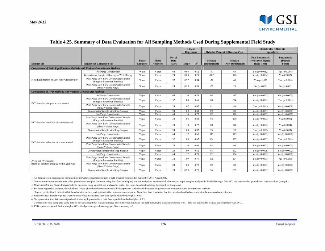
May 2013
SERDP ER-1601 126 Final Report
Table 4.25. Summary of Data Evaluation for All Sampling Methods Used During Supplemental Field Study
Sample Set Sample Set Compared to: Phase
Sampled Phase
Analyzed
No. of Data Pairs
Linear Regression Relative Percent Difference (%)
Statistically Different? (p-value)
Slope R2 Median
(Directional) Median
(Non-Directional)
Non-Parametric (Wilcoxon Signed
Rank Test)
Parametric (Paired t-test)
Comparison of Field Equilibration Methods with Various Groundwater Methods
Field Equilibration of Low-Flow Groundwater
No-Purge Groundwater Water Vapor 64 0.96 0.82 -39 65 Yes (p=0.0012) Yes (p=0.008)
Groundwater Sample Following In-Well Mixing Water Vapor 24 0.88 0.70 -107 116 Yes (p=0.0004) Yes (0.0002)
Post-Purge Low-Flow Groundwater Sample (Purge to Parameter Stability)
Water Vapor 32 0.97 0.94 -22 40 Yes (p=0.02) Yes (p=0.005)
Post-Purge Low-Flow Groundwater Sample (Fixed Volume Purge)
Water Vapor 24 0.99 0.98 -23 29 No (p=0.07) No (p=0.07)
Comparison of PVD Methods with Various Groundwater Methods
PVD installed at top of screen interval
No-Purge Groundwater Vapor Vapor 64 1.10 0.70 94 97 Yes (p<0.0001) Yes (p<0.0001) Post-Purge Low-Flow Groundwater Sample
(Purge to Parameter Stability) Vapor Vapor 32 1.08 0.68 88 94 Yes (p<0.0001) Yes (p=0.001)
Post-Purge Low-Flow Groundwater Sample (Fixed Volume Purge)
Vapor Vapor 24 1.07 0.67 81 86 Yes (p=0.001) Yes (p=0.0008)
Groundwater Sample with Snap Sampler Vapor Vapor 24 1.08 0.84 89 89 Yes (p<0.0001) Yes (p<0.0001)
PVD installed at middle of screen interval
No-Purge Groundwater Vapor Vapor 64 1.10 0.72 101 110 Yes (p<0.0001) Yes (p<0.0001) Post-Purge Low-Flow Groundwater Sample
(Purge to Parameter Stability) Vapor Vapor 32 1.08 0.82 94 100 Yes (p=0.0003) Yes (0.0006)
Post-Purge Low-Flow Groundwater Sample (Fixed Volume Purge)
Vapor Vapor 24 1.10 0.72 80 84 Yes (p=0.0002) Yes (0.0004)
Groundwater Sample with Snap Sampler Vapor Vapor 24 1.08 0.87 93 95 Yes (p=0.002) Yes (0.0003)
PVD installed at bottom of screen interval
No-Purge Groundwater Vapor Vapor 64 1.12 0.63 115 119 Yes (p<0.0001) Yes (p<0.0001)
Post-Purge Low-Flow Groundwater Sample (Purge to Parameter Stability)
Vapor Vapor 32 1.09 0.67 104 107 Yes (p<0.0001) Yes (p=0.002)
Post-Purge Low-Flow Groundwater Sample (Fixed Volume Purge)
Vapor Vapor 24 1.10 0.60 93 93 Yes (p<0.0001) Yes (p<0.0001)
Groundwater Sample with Snap Sampler Vapor Vapor 24 1.09 0.82 98 102 Yes (p=0.0008) Yes (p=0.0002)
Averaged PVD results (from all samplers installed within each well)
No-Purge Groundwater Vapor Vapor 64 1.12 0.70 103 104 Yes (p<0.0001) Yes (p<0.0001) Post-Purge Low-Flow Groundwater Sample
(Purge to Parameter Stability) Vapor Vapor 32 1.09 0.73 100 104 Yes (p=0.0001) Yes (p=0.002)
Post-Purge Low-Flow Groundwater Sample (Fixed Volume Purge)
Vapor Vapor 24 1.08 0.73 82 82 Yes (p<0.0001) Yes (p<0.0001)
Groundwater Sample with Snap Sampler Vapor Vapor 24 0.93 0.75 96 97 Yes (p<0.0001) Yes (p<0.0001)
1. All data represent measured or calculated groundwater concentrations from a field program conducted in September 2011-August 2012.
2. Groundwater concentrations were either groundwater samples (collected using low-flow techniques) sent for analysis at a commercial laboratory or vapor samples analyzed in the field (using a field GC) and converted to groundwater concentrations (in mg/L).
3. Phase Sampled and Phase Analyzed refer to the phase being sampled and analyzed as part of the vapor-based methodology developed for this project.
4. For linear regression analyses, the calculated (vapor-phase based) concentration is the independent variable and the measured groundwater concentration is the dependent variable.
Slope of greater than 1 indicates that the calculated method underestimates the measured concentration. Slope less than 1 indicates that the calculated method overestimates the measured concentration.
5. Parametric test: Simple or paired t-test on mean of log-normalized data from specified methods (alpha = 0.05)
6. Non-parametric test: Wilcoxon signed rank test using log-normalized data from specified methods (alpha = 0.05)
7. Comparisons were completed using data for any constituent that was encountered above detection limits for the field instruments in each monitoring well. This was confined to a single constituent per well (VC).
8. PVD = passive vapor diffusion sampler; GC = field-portable gas chromatograph; NA = not analyzed.
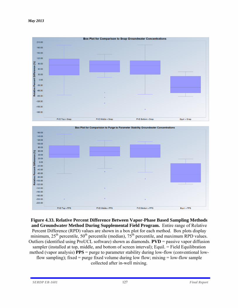
May 2013
SERDP ER-1601 127 Final Report
Figure 4.33. Relative Percent Difference Between Vapor-Phase Based Sampling Methods and Groundwater Method During Supplemental Field Program. Entire range of Relative Percent Difference (RPD) values are shown in a box plot for each method. Box plots display
minimum, 25th percentile, 50th percentile (median), 75th percentile, and maximum RPD values. Outliers (identified using ProUCL software) shown as diamonds. PVD = passive vapor diffusion
sampler (installed at top, middle, and bottom of screen interval); Equil. = Field Equilibration method (vapor analysis) PPS = purge to parameter stability during low-flow (conventional low-
flow sampling); fixed = purge fixed volume during low flow; mixing = low-flow sample collected after in-well mixing.
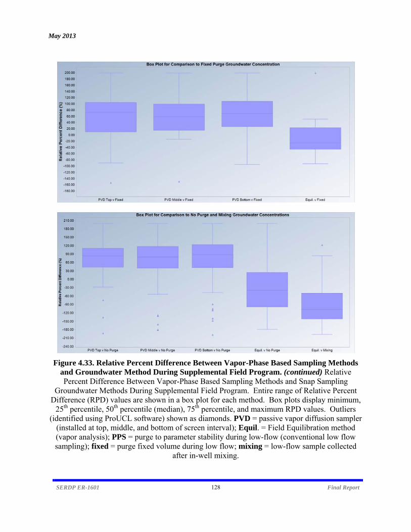
May 2013
SERDP ER-1601 128 Final Report
Figure 4.33. Relative Percent Difference Between Vapor-Phase Based Sampling Methods and Groundwater Method During Supplemental Field Program. (continued) Relative Percent Difference Between Vapor-Phase Based Sampling Methods and Snap Sampling
Groundwater Methods During Supplemental Field Program. Entire range of Relative Percent Difference (RPD) values are shown in a box plot for each method. Box plots display minimum,
25th percentile, 50th percentile (median), 75th percentile, and maximum RPD values. Outliers (identified using ProUCL software) shown as diamonds. PVD = passive vapor diffusion sampler
(installed at top, middle, and bottom of screen interval); Equil. = Field Equilibration method (vapor analysis); PPS = purge to parameter stability during low-flow (conventional low flow sampling); fixed = purge fixed volume during low flow; mixing = low-flow sample collected
after in-well mixing.
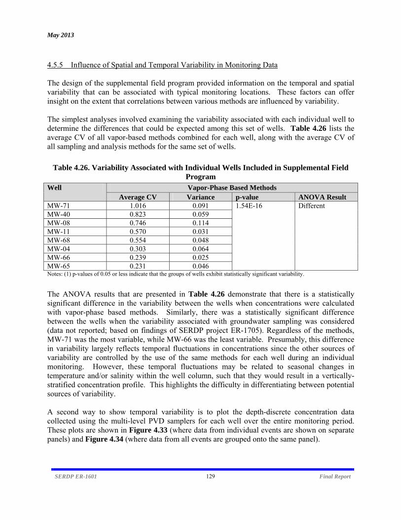
May 2013
SERDP ER-1601 129 Final Report
4.5.5 Influence of Spatial and Temporal Variability in Monitoring Data The design of the supplemental field program provided information on the temporal and spatial variability that can be associated with typical monitoring locations. These factors can offer insight on the extent that correlations between various methods are influenced by variability. The simplest analyses involved examining the variability associated with each individual well to determine the differences that could be expected among this set of wells. Table 4.26 lists the average CV of all vapor-based methods combined for each well, along with the average CV of all sampling and analysis methods for the same set of wells.
Table 4.26. Variability Associated with Individual Wells Included in Supplemental Field Program
Well Vapor-Phase Based Methods Average CV Variance p-value ANOVA Result
MW-71 1.016 0.091 1.54E-16 Different MW-40 0.823 0.059 MW-08 0.746 0.114 MW-11 0.570 0.031 MW-68 0.554 0.048 MW-04 0.303 0.064 MW-66 0.239 0.025 MW-65 0.231 0.046 Notes: (1) p-values of 0.05 or less indicate that the groups of wells exhibit statistically significant variability.
The ANOVA results that are presented in Table 4.26 demonstrate that there is a statistically significant difference in the variability between the wells when concentrations were calculated with vapor-phase based methods. Similarly, there was a statistically significant difference between the wells when the variability associated with groundwater sampling was considered (data not reported; based on findings of SERDP project ER-1705). Regardless of the methods, MW-71 was the most variable, while MW-66 was the least variable. Presumably, this difference in variability largely reflects temporal fluctuations in concentrations since the other sources of variability are controlled by the use of the same methods for each well during an individual monitoring. However, these temporal fluctuations may be related to seasonal changes in temperature and/or salinity within the well column, such that they would result in a vertically-stratified concentration profile. This highlights the difficulty in differentiating between potential sources of variability. A second way to show temporal variability is to plot the depth-discrete concentration data collected using the multi-level PVD samplers for each well over the entire monitoring period. These plots are shown in Figure 4.33 (where data from individual events are shown on separate panels) and Figure 4.34 (where data from all events are grouped onto the same panel).
May 2013
SERDP ER-1601 130 Final Report
Graphing the PVD data in this manner provides a visual indication of the extent of variability associated with each well. For example, Figure 4.35 clearly shows that the high variability associated with MW-71 (the most variable well based on the analysis presented in Table 4.26) is the result of large event-to-event changes in concentration, as opposed to stratified conditions that result in a wide range of concentrations across the sampling interval. Other wells such as MW-11 and MW-8 show evidence of spatial variability, where relatively higher concentrations are observed at one of the three depths during one or more events. Further, the shape of these concentration profiles at these wells changes over time.

May 2013
SERDP ER-1601 131 Final Report
Figure 4.34. All Concentration Data from PVD Samplers During Supplemental Field Program. Each box shows groundwater concentration (g/L) vs. location in the screen (PVD samplers were installed at the top, middle, and bottom of the screen interval). Boxes with three dots straight up and down represent near-uniform concentrations throughout the screened interval; boxes with staggered dots represent significant contaminant stratification. Blue-shaded cells represent events where conditions favor mixing (uniform concentrations) based on well-specific predictions by the soil temperature model. Overall, there did not seem to be a strong correlation between temperature stratification and contaminant stratification.
1/18/12
10/11/11
MW‐04 MW‐08 MW‐11 MW‐66 MW‐68 MW‐71
11/9/11
11/30/11
MW‐40 MW‐65
6/20/12
7/12/12
2/8/12
2/29/12
3/22/12
5/2/12
5/23/12
0 200,000 400,000 600,000
Depth
0 10,000 20,000
Depth
0 20,000 40,000 60,000
Depth
0 10,000 20,000
Depth
0 500,000 1,000,000
Depth
0 100,000 200,000 300,000
Depth
0 2,000 4,000 6,000
Depth
0 5,000 10,000
Depth
0 200,000 400,000 600,000
Depth
0 2,000 4,000
Depth
0 20,000 40,000 60,000
Depth
0 200 400
Depth
0 500,000 1,000,000
Depth
0 50,000 100,000 150,000
Depth
0 5,000 10,000
Depth
0 5,000 10,000
Depth
0 500,000 1,000,000
Depth
0 5,000 10,000
Depth
0 10,000 20,000 30,000
Depth
0 200 400
Depth
0 500,000 1,000,000
Depth
0 100,000 200,000 300,000
Depth
0 10,000 20,000
Depth
0 5,000 10,000
Depth
0 500,000 1,000,000
Depth
0 2,000 4,000 6,000
Depth
0 10,000 20,000
Depth
0 20 40Depth
0 500,000 1,000,000
Depth
0 100,000 200,000
Depth
0 5,000 10,000 15,000
Depth
0 50,000 100,000
Depth
0 500,000 1,000,000
Depth
0 2,000 4,000
Depth
0 10,000 20,000 30,000
Depth
0 2,000 4,000 6,000
Depth
0 500,000 1,000,000
Depth
0 100,000 200,000 300,000
Depth
0 5,000 10,000 15,000
Depth
0 50,000 100,000
Depth
0 500,000 1,000,000
Depth
0 1,000 2,000 3,000
Depth
0 50,000 100,000
Depth
0 20,000 40,000
Depth
0 500,000 1,000,000
Depth
0 500,000
Depth
0 50,000 100,000
Depth
0 200,000 400,000
Depth
0 200,000 400,000 600,000
Depth
0 2,000 4,000 6,000
Depth
0 20,000 40,000 60,000
Depth
0 5,000 10,000
Depth
0 200,000 400,000 600,000
Depth
0 100,000 200,000 300,000
Depth
0 10,000 20,000 30,000
Depth
0 50,000 100,000 150,000
Depth
0 500,000 1,000,000
Depth
0 5,000 10,000 15,000
Depth
0 20,000 40,000 60,000
Depth
0 500,000 1,000,000
Depth
0 100,000 200,000 300,000
Depth
0 10,000 20,000 30,000
Depth
0 10,000 20,000
Depth
0 100,000 200,000
Depth
0 500,000 1,000,000
Depth
0 20,000 40,000
Depth
0 50,000 100,000
Depth
0 10,000 20,000
Depth
0 500,000 1,000,000
Depth
0 200,000 400,000
Depth
0 20,000 40,000
Depth
0 100,000 200,000
Depth
0 500,000 1,000,000
Depth
0 10,000 20,000 30,000
Depth
0 50,000 100,000
Depth
0 5,000 10,000 15,000
Depth
0 200,000 400,000 600,000
Depth
0 200,000 400,000
Depth
0 20,000 40,000
Depth
0 50,000 100,000
Depth
0 500,000 1,000,000
Depth
0 20,000 40,000
Depth
0 50,000 100,000
Depth
0 5,000 10,000
Depth
0 200,000 400,000 600,000
Depth
0 100,000 200,000 300,000
Depth
0 10,000 20,000 30,000
Depth
0 10,000 20,000 30,000
Depth
Mixed
Stratified
Stratified
Stratified
Mixed
Mixed
Mixed
Mixed
Mixed
Mixed
Mixed
Stratified Stratified
Stratified Stratified Stratified Stratified Stratified
Stratified Stratified Stratified
Stratified
Stratified Stratified Stratified Stratified
Stratified Stratified Stratified Stratified
Stratified
Stratified Stratified
Stratified
Stratified Stratified Stratified
Stratified Stratified Stratified Stratified
Stratified
Stratified Stratified Stratified
Stratified Stratified Stratified
Stratified Stratified Stratified Stratified Stratified
Mixed Mixed Mixed Mixed Mixed
Mixed
Mixed
Mixed
Mixed Mixed
Mixed Mixed
Mixed Mixed
Mixed Mixed
Mixed Mixed Mixed
Mixed Mixed Mixed
Mixed Mixed
Mixed Mixed Mixed Mixed
Mixed Mixed
Stratified
Stratified
Stratified
Stratified
Stratified

May 2013
SERDP ER-1601 132 Final Report
Figure 4.35. Concentration Data from PVD Samplers During Supplemental Field Program Grouped by Event. Each box shows groundwater concentration (g/L) vs. location in the screen
(PVD samplers were installed at the top, middle, and bottom of the screen interval). Dates in the legend correspond to dates that individual monitoring events were completed.
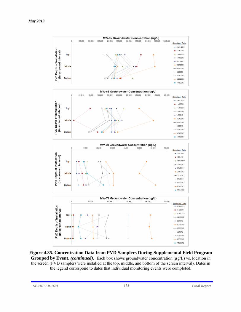
May 2013
SERDP ER-1601 133 Final Report
Figure 4.35. Concentration Data from PVD Samplers During Supplemental Field Program Grouped by Event. (continued). Each box shows groundwater concentration (g/L) vs. location in the screen (PVD samplers were installed at the top, middle, and bottom of the screen interval). Dates in
the legend correspond to dates that individual monitoring events were completed.

May 2013
SERDP ER-1601 134 Final Report
The presence of stratified concentrations within a monitoring well may result from poor in-well mixing. As described in Section 4.2, temperature-driven density gradients within a well can influence the degree of mixing that can be expected. Since these temperature gradients change seasonally, conditions favoring (or not favoring) mixing can exist at different periods within the same well. The expected mixing conditions within the set of wells used in the supplemental field program were determined using the soil temperature model presented in Section 3.2. In Figure 4.34, the shaded panels represent well and event combinations where mixing was favored based on the model predictions. The mixing predictions were then compared to variability associated with PVD-based concentrations in two ways:
1. The CVs for each well during each event were calculated to determine if the events where well-mixed conditions were predicted by the model were lower in variability than events where poorly-mixed (stratified) conditions were predicted by the model.
2. An index of stratification was calculated for each well for each event based on the ratio of the maximum depth-discrete concentration to the minimum depth-discrete concentration. The index of stratification for events where mixing was favored was then compared to the index of stratification for events where mixing was not favored.
The results of these analyses are presented in Table 4.27. For most wells, events where strong mixing was predicted were similar in terms of concentration stratification to events where stratification was favored. In about half the cases, wells were actually more stratified (i.e., higher values for the median CV and stratification index) during events where the prevailing temperature gradients would favor mixing.
Table 4.27. Evaluation of Stratification in Wells Included in Supplemental Field Program Well Median CV Median Stratification Index
(Higher is More Stratification) All
Events Events
Favoring Mixed
Conditions
Events Favoring Stratified
Conditions
All Events
Events Favoring
Mixed Conditions
Events Favoring Stratified
Conditions MW-71 0.09 0.04 0.13 1.2 1.1 1.4 MW-40 0.59 0.66 0.34 5.3 7.7 2.5 MW-08 0.78 0.57 0.97 5.4 4.8 16 MW-11 0.32 0.32 0.21 2.3 2.3 1.9 MW-68 0.12 0.10 0.15 1.3 1.3 1.3 MW-04 0.07 0.06 0.07 1.2 1.2 1.2 MW-66 0.19 0.24 0.15 1.6 1.8 1.4 MW-65 0.14 0.18 0.07 1.4 1.6 1.2 Notes: (1) A soil temperature model was used to predict whether conditions within each well during each event favored mixing
or stratification; (2) For each event and each well, a CV is calculated using the average and standard deviation of the three PVD concentrations. The median CV for each well over the course of all monitoring events is then reported; (3) For each event and each well, the Stratification Index is calculated as the ratio between the maximum and minimum concentration of the three PVD concentrations. The median CV for each well over the course of all monitoring events is then reported.
May 2013
SERDP ER-1601 135 Final Report
The calculated stratification indices for individual wells suggest that MW-40 and MW-08 exhibit the highest levels of stratification. However, this metric also demonstrates that—collectively—this set of wells displays relatively modest stratification. The difference between the maximum and minimum concentrations measured within a well was generally less than an order of magnitude (i.e., stratification index < 10). Out of the 88 concentration profiles obtained from this set of 8 wells, the stratification index exceeded 10 in only 7 instances (with 4 in MW-8 alone) and never exceeded 100.
The limited stratification observed during this field program may have resulted from relatively strong in-well mixing or may be a function of uniform concentrations within the depth intervals being targeted by the individual monitoring wells. The similarities between CVs for events that favored mixing with those that did not favor mixing would suggest that the latter is a more important factor for this set of wells. The finding that stratification was relatively limited provides supporting evidence for why relatively similar correlations were obtained when low-flow groundwater concentrations were compared with any of the PVD sampler-based concentrations. Regardless of where the sampler was installed, it was measuring water with similar concentration. At a site with less vertical uniformity in concentrations (or where conditions favoring in-well mixing were infrequent), the knowledge that a well tends towards spatial stratification during certain events may influence the selection of particular vapor-phase based monitoring methods (as well as groundwater-based methods). If depth-discrete concentration profiles are valuable components of a particular monitoring program, then multi-level passive samplers are the more appropriate choice. If the high concentration intervals of a stratified well are associated with less transmissive portions of an aquifer, then low-flow groundwater sampling (which tends to result in a flow-weighted average concentration) may not be representative. 4.6 Assessment of Cost-Effectiveness Relative to conventional groundwater sampling and testing methods currently in use at most DoD facilities, vapor-phase groundwater sampling methods represent a potentially large cost-savings because it eliminates several steps in the monitoring process (e.g., shipping of samples, analysis of samples at commercial laboratory). A preliminary estimate relative to standard groundwater sampling was prepared as part of the proposal, and it generated a savings of several hundred dollars per sample. Based on the greater than 100,000 groundwater samples estimated to be collected annually at Air Force, Army, and Navy installations in the U.S, savings of this magnitude correspond to a total savings of over $20 to 50 million per year. A more comprehensive assessment of the cost-effectiveness of this approach was prepared as part of the project. This includes comparisons between conventional groundwater monitoring and vapor-based methods, using unit costs (cost per sample) and total costs for various scenarios.
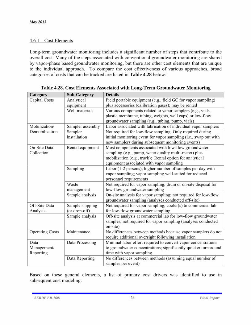
May 2013
SERDP ER-1601 136 Final Report
4.6.1 Cost Elements Long-term groundwater monitoring includes a significant number of steps that contribute to the overall cost. Many of the steps associated with conventional groundwater monitoring are shared by vapor-phase based groundwater monitoring, but there are other cost elements that are unique to the individual approach. To compare the cost effectiveness of various approaches, broad categories of costs that can be tracked are listed in Table 4.28 below:
Table 4.28. Cost Elements Associated with Long-Term Groundwater Monitoring Category Sub-Category Details Capital Costs Analytical
equipment Field portable equipment (e.g., field GC for vapor sampling) plus accessories (calibration gases); may be rented
Well materials Various components related to vapor samplers (e.g., vials, plastic membrane, tubing, weights, well caps) or low-flow groundwater sampling (e.g., tubing, pump, vials)
Mobilization/ Demobilization
Sampler assembly Labor associated with fabrication of individual vapor samplers Sampler installation
Not required for low-flow sampling; Only required during initial monitoring event for vapor sampling (i.e., swap out with new samplers during subsequent monitoring events)
On-Site Data Collection
Rental equipment Most components associated with low-flow groundwater sampling (e.g., pump, water quality multi-meter) plus mobilization (e.g., truck); Rental option for analytical equipment associated with vapor sampling
Sampling Labor (1-2 persons); higher number of samples per day with vapor sampling; vapor sampling well-suited for reduced personnel requirements
Waste management
Not required for vapor sampling; drum or on-site disposal for low-flow groundwater sampling
Sample analysis On-site analysis for vapor sampling; not required for low-flow groundwater sampling (analyses conducted off-site)
Off-Site Data Analysis
Sample shipping (or drop-off)
Not required for vapor sampling; cooler(s) to commercial lab for low-flow groundwater sampling
Sample analysis Off-site analysis at commercial lab for low-flow groundwater samples; not required for vapor sampling (analyses conducted on-site)
Operating Costs Maintenance No differences between methods because vapor samplers do not require additional oversight following installation
Data Management/ Reporting
Data Processing Minimal labor effort required to convert vapor concentrations to groundwater concentrations; significantly quicker turnaround time with vapor sampling
Data Reporting No differences between methods (assuming equal number of samples per event)
Based on these general elements, a list of primary cost drivers was identified to use in subsequent cost modeling:
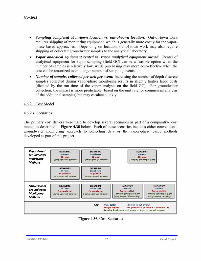
May 2013
SERDP ER-1601 137 Final Report
Sampling completed at in-town location vs. out-of-town location. Out-of-town work
requires shipping of monitoring equipment, which is generally more costly for the vapor-phase based approaches. Depending on location, out-of-town work may also require shipping of collected groundwater samples to the analytical laboratory.
Vapor analytical equipment rented vs. vapor analytical equipment owned. Rental of analytical equipment for vapor sampling (field GC) can be a feasible option when the number of samples is relatively low, while purchasing may more cost-effective when the cost can be amortized over a larger number of sampling events.
Number of samples collected per well per event: Increasing the number of depth-discrete samples collected during vapor-phase monitoring results in slightly higher labor costs (dictated by the run time of the vapor analysis on the field GC). For groundwater collection, the impact is more predictable (based on the unit rate for commercial analysis of the additional samples) but may escalate quickly.
4.6.2 Cost Model 4.6.2.1 Scenarios The primary cost drivers were used to develop several scenarios as part of a comparative cost model, as described in Figure 4.36 below. Each of these scenarios includes either conventional groundwater monitoring approach to collecting data or the vapor-phase based methods developed as part of this project.
Figure 4.36. Cost Scenarios
May 2013
SERDP ER-1601 138 Final Report
4.6.2.2 Assumptions Several assumptions were used to build the cost model. These assumptions include those that are directly related to the type of monitoring approach being employed (e.g., amount of time required to sample vapor vs. groundwater) as well as those that are shared by all approaches (e.g., number of wells sampled during each event).
All vapor-based sampling is completed using short PVDs, with associated costs for material and construction. Construction, assembly and installation of well materials can be completed by a technician (i.e., does not require engineer/geologist).
Vapor sampling requires an initial mobilization 3 weeks prior to the first event. New samplers are installed at the conclusion of monitoring events, such that separate mobilizations are not required for subsequent events. Samplers can be installed in 30 wells per 8 hour day.
Twenty wells are sampled during 15 different events (approximately 4 years of quarterly monitoring events).
Travel time to the site is 1 hour each way, with 8 hours available for on-site work. Groundwater sampling requires duplicates collected at a frequency of 1 in 10. Vapor
sampling requires duplicate analyses for every sample. Groundwater sampling requires two persons (entry-level field engineer/geologist plus
technician). Vapor sampling requires only one person (mid-level field engineer/geologist), though this person was assumed to have a slightly higher hourly rate (44%) than the entry-level field person required for conventional groundwater sampling. It is our experience that a mid-level field person can use the field GC with limited training, and that there is no need to contract an outside technical specialist to run the field GC.
Two gallons of water for disposal are generated per well per event for low-flow groundwater sampling.
GC analysis of vapor-phase samples requires 10 minutes per analyses (suitable for TCE with sufficient contingency for prepping instrument between analyses).
Out-of-town work necessitates shipping cooler(s) of groundwater samples to an analytical laboratory. For in-town work, coolers of groundwater samples could be dropped off at the analytical laboratory.
4.6.3 Results All of the scenarios examined under the cost model used a total of 20 sampling locations sampled for 15 discrete events, regardless of the sampling method. Results are presented in terms of total cost as well as cost per data point (i.e., concentration result from a single location or discrete depth). A summary of the results is provided in Table 4.29; complete results are presented in Table A.10 in Appendix A.

May 2013
SERDP ER-1601 139 Final Report
For all comparisons between relevant scenarios, the vapor-based monitoring method was less expensive than the groundwater monitoring method. This included the following:
Vapor-Based Sampling vs. Low-Flow Groundwater Sampling, In-Town with GC rental (Scenario 1 vs. 5): The vapor-based method cost $304 per sample while the groundwater method cost $473 per sample. This means that this program could be completed using vapor-phase monitoring at a discount of approximately 36% of the cost of conventional monitoring using low-flow groundwater sampling.
Vapor-Based Sampling vs. Low-Flow Groundwater Sampling, In-Town with GC purchase (Scenario 3 vs. 5): The vapor-based method cost $404 per sample while the groundwater method remained at $473 per sample. This means that for the monitoring program constructed for this modeling exercise, purchasing a dedicated GC for on-site vapor analyses increased costs by approximately 33% relatively to the rental option, but total costs for vapor-based monitoring remained well below those of conventional groundwater monitoring.
Vapor-Based Sampling vs. Low-Flow Groundwater Sampling, Out-of-Town with GC rental (Scenario 2 vs. 6): The vapor-based method cost $387 per sample while the groundwater method cost $617 per sample. The incremental costs of performing the vapor-phase method at an out-of-town location (e.g., equipment shipping) is outweighed by the additional expenses associated with two persons travelling for groundwater monitoring and shipping of sample coolers. Consequently, the vapor-based method remained approximately 37% cheaper.
Vapor-Based Sampling vs. Low-Flow Groundwater Sampling, Out-of-Town with GC purchase (Scenario 3 vs. 6): The vapor-based method cost $505 per sample while the groundwater method cost $617 per sample, meaning that purchasing a GC added approximately 30% to the cost of completing vapor-based monitoring at an out-of-town location (relative to GC rental) for this program.
Multi-Level Vapor-Based Sampling vs. Multi-Level Groundwater Sampling, In-Town with GC rental (Scenario 7 vs. 8 vs. 9): The vapor-based method cost $212 per sample to collect 3 depth-discrete samples per location. The groundwater methods cost $246 per sample using passive diffusion bags and $441 per sample using low-flow methods to collect the same number of groundwater samples per location. Therefore, the vapor-based method represents a cost savings of 14% relative to passive diffusion bags and 52% relative to low-flow methods for the same monitoring program.

May 2013
SERDP ER-1601 140 Final Report
Table 4.29. Summary of Cost Modeling Results Cost Element Scenario 1 Scenario 2 Scenario 3 Scenario 4 Scenario 5 Scenario 6 Scenario 7 Scenario 8 Scenario 9 Technology Type Vapor Vapor Vapor Vapor Low-Flow
GW Low-Flow
GW Vapor Passive Diffusion
Bag GW Low-Flow
GW
Travel Option In Town Out of Town
In Town Out of Town
In Town Out of Town
In-Town In-Town In-Town
On-site GC vs. Lab GC Rental GC Rental GC Buy GC Buy Lab Lab GC Rental Lab Lab
# of Samples per Location per event
1 1 1 1 1 1 3 3 3
Total Number of Samples (not including duplicates)
300 300 300 300 300 300 900 900 900
Prep and Sample Collection $53,850 $69,515 $53,850 $69,515 $77,210 $115,910 $114,415 $45,190 $204,540 Sample Analysis $11,440 $17,440 $37,640 $48,140 $44,515 $47,170 $24,640 $129,670 $134,970 Data Management and Reporting $13,980 $13,980 $13,980 $13,980 $13,980 $13,980 $26,980 $36,980 $36,980 Contingency (15%) $11,891 $15,140 $15,821 $19,745 $20,356 $26,559 $22,955 $31,776 $56,924 TOTAL COST $91,161 $116,075 $121,291 $151,380 $156,061 $203,619 $175,990 $243,616 $436,414 COST PER SAMPLE $304 $387 $404 $505 $473 $617 $212 $246 $441

May 2013
SERDP ER-1601 141 Final Report
(a) (b) (c)
Figure 4.37. Summary of Cost Sensitivity Analysis. (a) Sensitivity to number of samples per event; (b) Sensitivity to number of sampling events; and (c) Sensitivity to number of samples per location per event.
$‐
$200
$400
$600
$800
$1,000
$1,200
$1,400
$1,600
0 30 60 90 120
Cost per Sample
Number of Samples per Event
Scenario 1
Scenario 2
Scenario 3
Scenario 4
Scenario 5
Scenario 6
$‐
$500
$1,000
$1,500
$2,000
$2,500
$3,000
$3,500
0 30 60
Cost per Sample
Number of Sampling Events
Scenario 1
Scenario 2
Scenario 3
Scenario 4
Scenario 5
Scenario 6
$‐
$100
$200
$300
$400
$500
$600
$700
$800
$900
$1,000
0 2 4 6 8 10 12
Cost per Sample
Number of Samples Per Location Per Event
Scenario 7
Scenario 8
Scenario 9
May 2013
SERDP ER-1601 142 Final Report
4.6.4 Sensitivity Analysis The sensitivity of cost estimates to changes in the several of the cost elements was evaluated, with the results shown in chart form (Figure 4.37). In the context of the scenarios described in the previous section, this sensitivity exercise provides broader cost information that can be used for site-specific monitoring concerns. 4.6.4.1 Sensitivity to Total Number of Samples Groundwater sampling is cheaper than vapor-based sampling only for the case when the program is completed in town and the number of samples is exceedingly low (5 or less). This is due to the rental charge for the field GC (estimated as $400/day) outweighing the collection and analysis cost savings associated with the vapor-phase method. When the program is completed out-of-town, vapor-based monitoring is always cheaper than groundwater monitoring, regardless of the number of samples. Increasing the total number of samples included in a monitoring program (either through increasing the number of samples per event or the number of events) decreases the unit cost, regardless of the sampling and analysis methods. However, the unit costs decrease much more sharply for vapor-based methods than for groundwater methods in all cases. For in-town programs, vapor-phase sampling becomes cheaper than groundwater sampling once the number of samples per event is greater than 5. Once this number exceeds 15 samples per event, then purchasing a dedicated field GC (as opposed to renting) becomes more cost-effective than groundwater sampling. Once the number of samples per event reaches 100, then the GC purchase option becomes cheaper than the GC rental option. These limits are slightly smaller when out-of-town programs are considered. While a program with 100 wells is relatively large, it is certainly not uncommon to have more than 100 wells at sites with extensive long-term monitoring program and potentially multiple areas of concern. The cost charts demonstrate that the modeling results presented in Table 4.29 are generally representative of typical monitoring programs. The input values (i.e., 20 samples per event, 15 events) are generally near the point where most of the cost curves begin to level off. Beyond these points, unit costs decrease incrementally but the overall cost savings are relatively modest. 4.6.4.2 Sensitivity to Number of Samples Collected Per Well Per Event Vapor-based methods are well-suited for conducting multi-level sampling because the simplest samplers are small and can easily be strung with a monitoring well. The vapor-based methods (Scenario 7) proved to be cheaper than collecting groundwater samples using passive diffusion bags (Scenario 8) or low-flow techniques (Scenario 9) whether a single or multiple samples per well were required. The cost savings are largely attributable to reduced analytical costs associated with vapor-based methods, where all analyses are completed in the field at a relatively rapid rate. Therefore, increasing the number of samples per well does not increase the total cost

May 2013
SERDP ER-1601 143 Final Report
significantly and results in modest improvements in unit costs ($ per sample). A similar pattern is seen with passive groundwater diffusion bags, but for a different reason. These bags are easy to install, retrieve, and sample, such that the costs associated with sample collection are very low, regardless of the number of samples. Therefore, the unit costs for passive diffusion bags are relatively constant and largely tied to analytical costs. As the number of samples per well increases to 10, low-flow groundwater sampling becomes more cost-comparable to the other methods. However, this is a large number of depth-discrete samples for a single location and would require extensive well infrastructure (i.e., nested monitoring wells, packers) that is likely impractical at most sites. Consequently, using the vapor-based methods for multi-level sampling results in the lowest unit cost of any of the cost scenarios examined here ($150 to $300 per datapoint).
May 2013
SERDP ER-1601 144 Final Report
5. CONCLUSIONS AND IMPLICATIONS FOR FUTURE RESEARCH/IMPLEMENTATION
5.1 Key Conclusions
1. Existing commercially available field-portable vapor-phase monitoring equipment is sufficiently accurate, precise, and sensitive for calculating equivalent VOC concentrations in groundwater down to part per billion levels.
2. A field-portable GC demonstrated the highest performance of the analytical devices that were tested. Simple PID instruments did not work well for this application.
3. Vapor-phase sampling and analysis methods are easy to implement and can be tailored to site-specific needs.
4. Collecting vapor samples from a sealed monitoring well headspace was not an effective method for determining groundwater concentrations under the tested conditions due to stratification in wells (see #8).
5. VOC groundwater concentrations can be reasonably and reliably estimated using submerged passive vapor samplers. Both a simple passive vapor sampler constructed of a 40-mL vial in plastic and two longer samplers (including the Haas Balloon Sampler) worked well. Field equilibration of conventional collected groundwater samples followed by on-site vapor analysis using a field GC also worked well.
6. Vapor-phase based monitoring methods are no more variable than conventional groundwater monitoring methods, including low flow sampling.
7. Although not a strong factor in this study, seasonal temperature gradients have the potential to significantly alter monitoring data, including both conventional and vapor-phase based methods. These effects are much more pronounced in shallow wells but are likely minimal in wells deeper than approximately 15 to 20 m bgs.
8. Vertical stratification can be important contributing factor to variability and limits the utility of the well-headspace vapor-phase-based monitoring approach.
9. Other well and aquifer-specific factors can contribute to variability and influence the performance of vapor-phase based monitoring methods.
10. Passive vapor sampling methods represent a very promising approach for field-based estimation of groundwater concentrations.
11. Vapor-phase based methods represent a significant cost savings (36% or more) relative to conventional groundwater monitoring approaches.

May 2013
SERDP ER-1601 145 Final Report
5.2 Discussion The overall objective of this research project was to evaluate the utility of on-site analysis of well headspace and other vapor-phase samples as an alternative to off-site analysis of groundwater samples. Currently, monitoring programs employed by the DoD (and most non-federal stakeholders) rely heavily on 25 to 30-year old techniques, and must go through multiple steps of collection, handling, lab analysis, and data transfer before the results reach the intended audience. The opportunity for significant cost savings exists if alternative long-term monitoring approaches are developed that can reduce the number of steps in traditional sampling programs by making use of improved knowledge and technologies for sample analysis. The development of reliable vapor-phase-based monitoring approaches is designed to aid the DoD with several key goals in long-term monitoring optimization. First, it entails a less cost and time-intensive method for analyzing specific contaminants of concern, including all chlorinated hydrocarbons. Further, it can utilize inexpensive and cost-effective tools during the data collection process. Finally, it represents a simple approach that would be easy to implement at a majority of DoD sites nationwide. All of these factors work to significantly reduce the cost liabilities associated with groundwater monitoring while providing a more sustainable long-term approach. The principle driving this research is that the VOC concentration measured in a vapor-phase sample that is in equilibrium with affected groundwater can be used to accurately determine the VOC concentration in the associated groundwater at or below MCLs. Two key hypotheses were developed to support this principle: (1) Portable vapor-phase monitoring instruments can be used to accurately determine VOC concentrations in water under equilibrium conditions; (2) In-well mixing is sufficient in some or all groundwater monitoring wells to establish equilibrium partitioning conditions between affected groundwater and in-well headspace vapors. To test these hypotheses and validate the use of in-field vapor-phase groundwater monitoring techniques, the specific technical objectives of the project were as follows:
1. Validate the use of field-portable vapor phase monitoring equipment to determine VOC concentration in water samples by conducting a detailed laboratory study.
2. Evaluate several different sampling methods to obtain vapor-phase samples in equilibrium with groundwater at the monitoring well.
3. Evaluate the accuracy, precision, and sensitivity of field-based, vapor-phase groundwater monitoring compared to existing groundwater monitoring technologies.
4. Identify conditions where equilibrium partitioning occurs between groundwater and well head space vapors by performing statistical evaluations of the contribution of a variety of aquifer and well construction characteristics to sampling variability.
5. Develop practical guidelines for the selection of appropriate vapor-phase groundwater monitoring strategies for various settings and applications (aquifer type, detection
May 2013
SERDP ER-1601 146 Final Report
monitoring programs, natural attenuation monitoring programs, etc.), including cost-effectiveness.
Data to address these objectives were collected through a series of testing programs, consisting of: i) a laboratory-based study to validate analytical equipment and to identify promising methods; ii) three distinct phases of field-based studies (preliminary, expanded, and supplemental) to test various sampling and collection methods and to examine design and well-specific factors that influenced performance; and iii) a combined modeling-field study that focused on the influence of seasonal temperature gradients on vertical stratification of concentration within monitoring wells. The major findings of these studies are presented below, focusing on the specific project objectives which they were designed to address: Existing commercially available field-portable vapor-phase monitoring equipment are sufficiently accurate, precise, and sensitive for calculating equivalent VOC concentrations in groundwater down to part per billion levels (OBJECTIVE #1.) Vapor-phase analytical equipment was validated as part of the detailed laboratory study (see Section 4.1 for results). During these lab tests, both a field-portable GC and a PID met nearly all accuracy and precision goals for vapor sample analysis, including in the presence of a water phase where the concentration was calculated using equilibrium partitioning. For both instruments, sensitivity was less than the MCL for three different VOCs that were evaluated. Based on these results, vapor analysis conducted using a field portable instrument can be used to measure VOC concentrations in water with sufficient accuracy, precision, and sensitivity to achieve typical groundwater monitoring objectives. A field-portable GC demonstrated the highest performance of the analytical devices that were tested. Simple PID instruments did not work well for this application (OBJECTIVES #1 and #3). Using the field GC, strong correlations between vapor and groundwater concentrations were established during field testing as long as samples were from the same depth interval and were collected using similar techniques. The PID performed well during the laboratory study, but it proved unreliable during field testing in terms of both accuracy and precision (see Section 4.3 and 4.4 for results). While this instrument provides some benefits in terms of simplicity and familiarly (i.e., most personnel involved in environmental monitoring have used this type of device), these benefits did not outweigh the observed compromise in data quality (relative to the more reliable field GC). Determining the equivalent groundwater concentration from a PID vapor-phase measurement relies on several factors (e.g., instrument correction factors, some knowledge of relative ratios of constituents present in the sample, high volume requirements, overcoming influence of humidity). Collectively, these factors contributed significant variability and bias (specifically, underprediction of the actual groundwater concentration) when the PID was used in the field. Another alternative field instrument for vapor-phase analysis—the HAPSITE with GC/MS capabilities—was also tested (see Section 4.4 for results). This instrument did not perform as strongly as the simpler field GC with respect to accuracy and
May 2013
SERDP ER-1601 147 Final Report
precision, although it did prove useful in terms of identifying a higher number of constituents at lower detection limits. The field GC has the distinct advantage of requiring only very limited sample volumes (100 L or less), such that it can be used in conjunction with small (depth-discrete) vapor samples. Vapor-phase sampling and analysis methods are easy to implement and can be tailored to site-specific needs (OBJECTIVE #2). Several vapor-phase sampling approaches were initially tested during the lab study and then evaluated in a more comprehensive manner during one or more subsequent field trials. In all cases, the methods involved simple approaches with minimal equipment that was easily adaptable to existing monitoring wells. All methods rely on a cap that seals the vapors within the monitoring well, with the simplest method installing ports within the cap that allow for sampling the headspace above the water level. Several methods were tested that involved submerging a passive vapor sampling device below the water level, typically near the screened interval of the well. These water-tight samplers are filled with gas and wrapped with thin low-density polyethylene that permits gas—but not water—cross. As a result, the gas within the sampler reaches equilibrium with the surrounding groundwater, typically in less than a few weeks. Several passive sampler designs were tested, including short samplers based on 40-mL vials (for depth-discrete sampling) and longer devices designed to cover larger portions of the screened interval. These passive samplers were all easy to construct from readily available materials, with a common requirement being the use of a weighted line during deployment to ensure submersion. A final sampling method involved the field vapor analysis of a groundwater sample that had been equilibrated in the field (for 60 minutes or less). This represented a simple modification of typical low-flow groundwater sampling with the distinct advantage of generating the data on-site. While the performance of the various sampling and analysis methods that were tested differed somewhat, each had strong points that may lend themselves to certain monitoring applications more readily than others (see below for further discussion). Collecting vapor samples from a sealed monitoring well headspace was not an effective method for determining groundwater concentrations under the tested conditions due to stratification in wells (OBJECTIVE #3). Evaluating the performance of the various vapor-phase based methods for determining groundwater concentrations was the focus of the various phases of field testing., and the simple headspace method was tested during the preliminary field program (see Section 4.3 for results). Strong correlations between groundwater concentrations calculated using these headspace samples—from either the upper portion of the well or the water-vapor interface—and lab-analyzed groundwater samples could not be established. Vapor-phase measurements were consistently biased low with high variability. The results indicate that the vapor sample that was collected from the well headspace was in equilibrium with water that was typically not representative of the water collected for low-flow sampling. However, there was clear consistency between the data collected from the upper headspace and the interface, confirming that diffusion in the air column is rapid and that the headspace sampling location is not an important contributor to variability.

May 2013
SERDP ER-1601 148 Final Report
VOC groundwater concentrations could be most reasonably and reliably estimated using submerged passive vapor samplers. Both a simple passive vapor sampler constructed of a 40-mL vial in plastic and two longer samplers worked well. Field equilibration of conventional collected groundwater samples followed by on-site vapor analysis using a field GC also worked well (OBJECTIVE #3). The passive vapor diffusion (PVD) samplers consistently generated data that was strongly correlated with data from passive water samplers and low-flow groundwater samples. Correlations obtained during each of the phases of field testing were relatively similar (R2 from linear regression typically > 0.85), with some evidence of a slight high bias (e.g., overprediction of actual groundwater concentrations). The passive vapor samplers rely on diffusion to ensure equilibrium, and thus correlated most strongly with similar groundwater sampling approaches, including passive groundwater diffusion bags (see Section 4.3 for results) and Snap samplers (see Section 4.5 for results). Collecting vapor samplers within the screened interval of the monitoring well—as opposed to the well headspace—helped to minimize the influence of stratification. The field equilibration method correlated very strongly with low-flow groundwater sampling data, which was expected since both methods quantify contaminants derived from the same source (i.e., collected groundwater). In these cases, the field equilibration method generated R2 values of 0.94 to 0.99 (depending on the field program), with a slight low bias observed only during the last (supplemental) phase of field testing. Vapor-phase based monitoring methods are no more variable than conventional groundwater monitoring methods, including low-flow sampling (OBJECTIVES #3 and #4). The variability of concentration data obtained using passive vapor diffusion samplers and the field equilibration method were evaluated during the last (supplemental) phase of field testing (see Section 4.5 for results). During several events completed over the course of nearly a year, the vapor-based methods demonstrated similar variability as various methods based on direct groundwater sampling and analysis (median CV values typically 0.5 – 0.7). No statistically significant differences in variability were obtained when comparing the vapor-phase based data with data obtained using low-flow groundwater sampling (including no-purge samples, samples collected after in-well mixing, samples collected after purging fixed volumes, and samples collected after purging to parameter stability) or Snap samplers (i.e., passive groundwater samplers). In general, methods designed to reduce variability had little or no significant benefit. These results confirm that—for this set of wells—the temporal variability observed in the monitoring data is primarily associated with signal variability, and that the vapor-phase methods do not introduce significant additional variability that would hinder assessments of concentration trends. Although not a strong factor in this study, seasonal temperature gradients have the potential to significantly alter monitoring data, including both conventional and vapor-phase based methods (OBJECTIVES #4 and #5). A simple model was used to demonstrate the changing influence of temperature on the degree of mixing that can occur within a monitoring well (see Section 4.2 for results). During warmer periods, the temperature of water near the surface is higher than at deeper depths, meaning that less dense (warmer) water overlies more dense (cooler) water within the well. If contaminant concentrations in the aquifer are also stratified, then the thermally stratified conditions can help to maintain vertical stratification of

May 2013
SERDP ER-1601 149 Final Report
contaminants within the well. The opposite pattern occurs during cooler periods, when a reversed temperature gradient can promote in-well mixing. The influence of temperature gradients depends on the depth of the well screen, with the model showing that shallow wells are particularly susceptible. Depending on the local climate (specifically the difference between the annual mean temperatures during winter and summer), these temperature effects appear to be negligible in wells deeper than approximately 15 to 20 m bgs. The model predictions were validated in a limited-scale field study that showed that vertical stratification of concentration (i.e., 100x difference between depth-discrete concentrations) occurred in a period when the measured temperature profile favored stability and that uniform concentrations were observed during a period when the temperature profile favored in-well mixing. The fact that conditions within an individual well may shift over time—between conditions that favor in-well mixing and conditions that favor stratification—means that properly-designed monitoring programs must understand the level of expected stratification within their monitoring network. Without this knowledge, establishing long-term concentration trends may be difficult due to the variability associated with conventional monitoring approaches within stratified wells.
Vertical stratification can be important contributing factor to variability and limits the utility of well headspace vapor-phase-based monitoring approach (OBJECTIVE #4). The temperature study demonstrated that the monitoring wells that were part of the field programs were potentially subject to temperature gradients that could contribute to vertical stratification and/or in-well mixing. During the various phases of field testing, the clearest indication of the influence of vertical stratification came during the preliminary field program where concentrations measured in water samples collected from the interface were significantly different than those from samples collected from the screened interval. This indicated that the water column within the monitoring wells was poorly mixed in a significant number of wells included in the study. This stratified condition negatively influences the ability to collect a well headspace sample that is representative of low-flow groundwater concentration because the air column is in equilibrium with a water concentration that is different from that at the screen. As a result, the headspace method is generally deemed unreliable unless there is evidence that stratification is not an issue in the wells being monitored. It is important to note that during other phases of field testing, there was less evidence of vertical stratification within wells. For instance, the fact that passive vapor samplers of varying length (i.e., covering different portions of the screened interval) demonstrated similar performance during the expanded field program indicated that stratification was not strong during that particular monitoring period. Even stronger evidence was obtained during the supplemental field program where passive vapor samplers were placed at multiple depths within the screened interval of the 8 wells that were part of the program. The data from these depth-discrete samplers showed that the majority of wells exhibited fairly uniform concentrations with depth, as well as similar variability for events that favored mixing with those that did not favor mixing. As a result, relatively similar correlations were obtained when low-flow groundwater concentrations were compared with any of the PVD sampler-based concentrations because, regardless of where the sampler was installed, it was measuring water with similar concentration.
May 2013
SERDP ER-1601 150 Final Report
Other well and aquifer-specific factors can contribute to variability and influence the performance of vapor-phase based monitoring methods (OBJECTIVE #4). In addition to the potential for in-well mixing (driven by temperature or solute gradients that influence density), other well and aquifer-specific factors were investigated during the preliminary field program (see Section 4.3 for results) and the expanded field program (see Section 4.4 for results). Using an ANOVA-based approach to evaluate the data, the majority of these factors had little statistically significant impact on the performance of the vapor-phase based methods. This included the distance between the top of the aquifer and the well screen, the depth to the top of the aquifer, the dissolved oxygen concentration, and large changes in geochemical parameters during purging. One factor that appeared to have a significant influence was the presence or absence of confining conditions within the aquifer being monitored. It was hypothesized that wells in unconfined wells could exhibit more variability due to the potential influence of fluctuating water levels on contaminant concentrations. However, the results showed that for this set of wells, better performance was obtained when the vapor-phase-based methods were employed in unconfined aquifers. This is based primarily on improved R2 values and slopes that are consistently closer to one (indicating less bias). Using the most reliable analytical instrument (the field GC), slopes were typically well below one for datasets from confined wells, indicating that concentrations were consistently underpredicted. Passive methods represent a very promising approach for field-based estimation of groundwater concentrations (OBJECTIVE #5). Passive vapor sampling did not suffer from the same degree of bias or variability as direct headspace sampling. In particular, passive methods are not as reliant as headspace sampling on in-well mixing, and in fact are well-suited to examine vertical stratification within the well. Deployment is straightforward and based on the same protocol as conventional passive water samplers, while offering the distinct advantage of rapidly-generating data in the field. A correction for the difference in pressure between deployment (i.e., when subject to hydrostatic pressure) and sample analysis is necessary if the samplers are expandable or if pressure-lock syringes are not used. In addition to the simple “short” passive vapor diffusion sampler, several more advanced passive sampler designs were also tested. This included a 5-ft long sampler that covered a much larger portion of the screened interval, and a slightly shorter, 2.5-ft long “balloon” sampler that was inflated during installation so that it could be sampled without retrieving it from the well. However, both of these designs performed very similarly to the simpler short PVDs in terms of correlations to groundwater concentrations (R2 = 0.85 – 0.89), presumably because the wells were not particularly stratified. It is assumed that these longer PVD sampler designs would provide stronger correlations than short PVDs in certain scenarios. However, their higher failure rate (e.g., collapsing or leaking when deployed in the water column) means that the simpler short PVD samplers may be more appropriate in some cases. For example, the short PVD samplers can be installed in series along the entirety of the screened interval to provide information on vertical stratification at minimal additional cost. Vapor-phase based methods represent a significant cost savings relative to conventional groundwater monitoring approaches (OBJECTIVE #5). A cost model was developed to compare vapor-phase based monitoring to conventional groundwater-based monitoring. The
May 2013
SERDP ER-1601 151 Final Report
model was tested using several scenarios, and in all cases, the vapor-phase based methods proved cheaper than the conventional methods. This included a cost savings of at least 36% when on-site vapor-based monitoring was completed using a rented GC. For these scenarios, this represents a savings of $100 to $250 per sample (depending on whether monitoring was completed at an in-town or out-of-town site). Sensitivity analysis was used to examine the impact of the number of samples per event and per well on overall cost. In particular, using passive vapor samplers to perform multi-level monitoring (i.e., increasing the number of samples per location) shifts the economics sharply in the favor of vapor-phase based methods. The findings described above demonstrate that, collectively, the project met all of the stated objectives. Of the original hypotheses, the first hypothesis—that portable vapor-phase monitoring instruments can be used to accurately determine VOC concentrations in water under equilibrium conditions—was validated by the project findings. However, the second hypothesis—that in-well mixing occurs at a high enough frequency to merit the use of headspace sampling—was not validated. Instead, submerged passive samplers, or an alternative field equilibration method, are the most appropriate vapor-phase-based methods in most cases. These approaches can be tailored for sites where a typical flow-weighted average concentration is desired, or for sites where depth-discrete concentration data are preferred. Primary research questions that remain include the following:
Understanding the specific reasons why certain factors contributed to decreased performance of vapor-phase based methods. The vast majority of well and aquifer-specific factors had no apparent effect, or at least their contributions did not result in statistically significant differences. One exception that is of particular interest is the negative influence of confining conditions on calculated groundwater concentrations. This ran counter to the original hypothesis that unconfined aquifers would result in more variable data because of the influence of fluctuating water levels. The poorer performance within confined aquifers was identified during the expanded field program. Further investigations in controlled (lab) settings would be useful in determining the underlying contributing factors. In addition, there were several well and aquifer-specific factors that could not be evaluated more fully because of limitations in the set of monitoring wells included in the various field programs. This includes the potential impact of clogging within older cast-iron wells on the variability associated with vapor-phase monitoring methods (all of the wells were stainless steel or PVC/HDPE). In general, clogging was not an issue within this set of monitoring wells. Low dissolved oxygen levels can be used as a proxy of biofouling (i.e., due to excessive microbial growth and/or formation of reduced iron and sulfide precipitates). During the project-specific field trials, the dissolved oxygen levels in wells had no statistically significantly impact on the results.
Identify why the PID performed poorly in multiple field trials. The PID worked well during the lab study and demonstrated sufficient accuracy and precision for most
May 2013
SERDP ER-1601 152 Final Report
monitoring applications. It did not meet expectations during the two field testing phases where it was employed, and poor performance was noted even in wells where a single constituent dominated. While limited testing was performed during the lab study that was part of this project, additional systematic testing of various PID operating parameters could provide insight and improve the overall utility of the PID. This would include testing the impact of humidity (and various humidity filters), intake rates and volumes, and response tests over wider ranges to better understand calibration effectiveness. We are aware of PID applications for quantifying non-aqueous phase and dissolved phase petroleum hydrocarbons in monitoring wells at underground storage tank sites. This work has been performed by Chevron but has yet to be published in the scientific literature. In discussions with Chevron personnel, they found certain models seemed to work better for this purpose. If nothing else, these parallel studies show that the PID has value in certain cases (e.g., bulk hydrocarbon detection).
Expanding our understanding of the prevalence of vertical stratification within monitoring wells. There was considerable evidence that a significant number of wells included in some phases of field testing were vertically stratified. However, the most extensive investigation of stratification was performed as part of the final phase (i.e., the supplemental field program). In this set of wells, depth-discrete concentrations were generally uniform within the majority of wells, such that the predicted temperature gradients had little observable impact on the extent of stratification at various points in the monitoring period. It would be insightful to expand studies on well stratification to a larger and more diverse set of wells to further confirm if patterns matched expectations based on temperature (or solute) driven gradients. This phenomenon has significant implications for the accuracy of both conventional and vapor-phase based monitoring methods. In particular, it impacts how representative the sampling result is of conditions in the surrounding aquifer.
The vapor-phase monitoring methods are straightforward and can be implemented by DoD and other stakeholders with limited additional training and expense (particularly using the attached guidance in Appendix C). Consequently, there are no technical limitations for its larger-scale use. While the studies completed as part of this project were conducted under rigorous QA/QC methodologies, these efforts did not involve interaction between DoD workgroups and regulatory entities. Proposed field trials at DoD sites were ultimately not performed for several reasons: i) there was significant work entailed in identifying and testing various sampling and analysis methods (particularly once the simple headspace method proved to be less reliable) that made it difficult to design and implement technically-sound and cost-effective larger-scale field programs; and ii) it was more practical to plan several phases of smaller-scale field trials at local commercial sites than to attempt to coordinate field work at DoD sites that had the potential to temporarily interfere with on-going long-term monitoring programs. The principal investigators for this project feel that there is a good opportunity to bridge the vapor-based monitoring approach from an experimental technique to a validated and regulator
May 2013
SERDP ER-1601 153 Final Report
approved monitoring method through various processes that would involve participation of DoD’s Environmental Data Quality Workgroup (EDQW) as well as regulatory entities. Efforts would be aimed at developing a sampling strategy in line with input and recommendations from the EDQW to assure that data obtained during monitoring events conforms with the data quality objectives necessary for successful validation. These efforts are well-suited as a follow-on project for ESTCP.
May 2013
SERDP ER-1601 154 Final Report
6. LITERATURE CITED
Adamson, D.T., T.E. McHugh, M.R. Rysz, and C.J. Newell, 2009. “Laboratory Validation Study
of New Vapor-Phase-Based Approach for Groundwater Monitoring”, Remediation, Winter 2009, 20(1): 87-106.
Adamson, D.T., T.E. McHugh, M.R. Rysz, R.C. Landazuri, and C.J. Newell, 2012. “Field Investigation of Vapor-Phase-Based Groundwater Monitoring”, Ground Water Monitoring & Remediation , Winter 2012, 32(1): 59-72.
ASTM, 2002. ASTM D6771-02 Standard Practice for Low-Flow Purging and Sampling for Wells and Devices Used for Ground-Water Quality Investigations. American Society of Testing Materials, January 2002
Barcelona, M.J., M.D. Varljen, R.W. Puls, and D. Kaminski. 2005. “Ground Water Purging and Sampling Methods: History vs. Hysteria”. Ground Water Monitoring & Remediation. Vol. 25 (3): 73-81.
Barker, J.F., and R. Dickhout, 1988. An Evaluation of Some Systems for Sampling Gas-Charged Ground Water for Volatile Organic Analysis. Ground Water Monitoring & Remediation, Fall 1988, Vol. 8(4): 112-120.
Britt, S.L., 2005. “Testing the In-Well Horizontal Laminar Flow Assumption with a Sand-Tank Well Model”. Ground Water Monitoring & Remediation, Vol. 25 (3): 73-81.
Britt, S.L., B.L. Parker, and J.A. Cherry, 2010. “A Downhole Passive Sampling System to Avoid Bias and Error from Groundwater Sample Handling”. Environmental Science & Technology, Vol. 44 (13): 4917-4923.
Church, P. E. and G. E. Granato. 1996. “Bias in Ground-Water Data Caused by Well-Bore Flow in Long-Screen Wells”. Ground Water. Vol. 34(2): 262-273.
Divine, C.E., and J.E. McCray, 2004. “Estimation of Membrane Diffusion Coefficients and Equilibration Times for Low-Density Polyethylene Passive Diffusion Samplers”. Environmental Science & Technology, 38(6): 1849-1857.
Divine, C.E., L.L., Madsen, S.D. Andres, and T. Santangelo-Dreiling, 2005. “Passive Diffusion Ground Water Samplers at a Site with Heterogeneous Hydrostratigraphy: Pilot Study Results”. Ground Water Monitoring & Remediation, 25(1), 90-99.
Elci, A., F.J. Molz III, and W.R. Waldrop, W.R., 2001. “Implications of Observed and Simulated Ambient Flow in Monitoring Wells”. Ground Water, 39(6), 853-862.
Gardner, P., and D.K. Solomon, 2009. An advanced passive diffusion sampler for the determination of dissolved gas concentrations. Water Resources Research, Vol. 45(6).
Guilbeault, M.A., B. L. Parker, and J. A. Cherry. 2005. “Mass and Flux Distributions from DNAPL Zones in Sandy Aquifers”, Ground Water. Vol. 43(1): 70-86.
Huffman, R.L. 2002. Comparison of Passive Diffusion Bag Samplers and Submersible Pump Sampling Methods for Monitoring Volatile Organic Compounds in Ground Water at Area 6, Naval Air Station Whidbey Island, Washington, U.S. Geological Survey WRIR-02-4203.
May 2013
SERDP ER-1601 155 Final Report
Hunter, P., 2004. Overview of Air Force Long-Term Monitoring Optimization, Programs and Case Studies. U.S. Air Force Center for Environmental Excellence, Brooks AFB, Texas. www.clu-in.org/siteopt/proceedings_04/track_b/wed/18_hunter_philip.pdf
Hutchins, S.R. and S.D. Acree, 2000. “Ground Water Sampling Bias Observed in Shallow, Conventional Wells”, Ground Water Monitoring & Remediation, Vol. 20 (1): 86-93.
ITRC, 2004. Technical and Regulatory Guidance for Using Polyethylene Diffusion Bag Samplers to Monitor Volatile Organic Compounds in Groundwater. Interstate Technology and Regulatory Council, Washington, D.C.: Diffusion Sampler Team.
ITRC, 2006. Technology Overview of Passive Sampler Technologies. Interstate Technology and Regulatory Council, DSP-4, Washington, D.C.: Diffusion Sampler Team.
ITRC, 2007. Protocol for Use of Five Passive Samplers to Sample for a Variety of Contaminants in Groundwater. Interstate Technology and Regulatory Council, DSP-5, Washington, D.C.: Diffusion/Passive Sampler Team.
Kampbell, D.H., and S.A. Vandegrift, 1998. “Analysis of Dissolved Methane, Ethane, and Ethylene in Ground Water by a Standard Gas Chromatographic Technique”. Journal of Chromatographic Science, Vol. 36: 253-256.
Kerfoot, H.B., and C.L. Mayer, 1986. “The Use of Industrial Hygiene Sampler for Soil-Gas Surveying”. Ground Water Monitoring & Remediation, Vol 6(4): 74-78.Martin-Hayden, J.M., 2000. “Sample Concentration Response to Laminar Wellbore Flow: Implications to Ground Water Data Variability”. Ground Water, Vol 38(1): 12-19.
Martin-Hayden, J.M., and N. Wolfe, 2000. “Sample Concentration Response to Laminar Wellbore Flow: Implications to Ground Water Data Variability”. Ground Water Monitoring & Remediation, Vol 20(4): 121-128.
Mayo, A.L., 2010. “Ambient well-bore mixing, aquifer cross-contamination, pumping stress, and water quality from long-screened wells: What is sampled and what is not?”. Hydrogeology Journal, Vol 18: 823-837.
McDonald, J.P. and R.M. Smith, 2009. “Concentration Profiles in Screened Wells under Static and Pumped Conditions”. Ground Water Monitoring & Remediation, Vol. 29 (2): 78-86.
McHugh, T.E., C.J. Newell, R.C. Landazuri, L.J. Molofsky, and D.T. Adamson, 2012. “The Influence of Seasonal Temperature Gradients on No-Purge Sampling of Wells”, Remediation, Autumn 2012, 22(4): 21-36.
McLeish, K., M.C. Ryan, and A. Chu, 2007. “Integrated Sampling and Analytical Approach for Common Groundwater Dissolved Gases”. Environmental Science & Technology, Vol 41: 8388-8393.
Metcalf, M.J., and G.A. Robins, 2007. “Comparison of Water Quality Profiles from Shallow Monitoring Wells and Adjacent Multilevel Sampler”. Ground Water Monitoring & Remediation, Vol 27(1): 84-91.
Minsker, B., 2003. Long-Term Groundwater Monitoring – The State of the Art. American Society of Civil Engineers, 2003.
Newell, C.J., R.S. Lee, and A.H. Sexpet, 2000. No-Purge Groundwater Sampling: An Approach
May 2013
SERDP ER-1601 156 Final Report
for Long-Term Monitoring. American Petroleum Institute Bulletin No. 12, October 2000.
Nofziger, D.L. & Wu, J. (2003). Soil Temperature Changes with Time and Depth Software. 2005.05.04, Retrieved May 4, 2003, from http://soilphysics.okstate.edu/software/SoilTemperature/
Parker, L.V., 1994. The Effects of Ground Water Sampling Devices on Water Quality: A Literature Review. Ground Water Monitoring & Remediation, Vol. 14(2): 130-141.
Parker, L., and Britt, S.L., 2012. “The Effect of Bottle Fill Rate and Pour Technique on the Recovery of Volatile Organics”. Ground Water Monitoring & Remediation, Vol. 32 (4): 78-86.
Paul, C.J., J. Wilson, and K. Jewell, 2007. A New Passive Diffusion Sampler (PDS) for Soil Gas Sampling. 17th Annual Association for Environmental Health and Sciences (AEHS) Meeting, March 21-22, 2007
Powell, R.M. and R.W. Puls. 1993. “Passive Sampling of Groundwater Monitoring Wells Without Purging: Multilevel Well Chemistry and Tracer Disappearance”. Journal of Contaminant Hydrology. Vol. 12: 51-77.
Puls, R.W. and M.J. Barcelona, 1996. Low-Flow (Minimal Drawdown) Ground-Water Sampling Procedures. United States Environmental Protection Agency, Office of Research and Development/Office of Solid Waste and Emergency Response, EPA/540/S-95/504.
Sammel, E.A.. 968.”Convective Flow and Its Effect on Temperature Logging in Small-Diameter Wells”. Geophysics, 33, 1004; doi: 10.1190/1.1439977.
Sanford, W.E., R.G. Shropshire, and D.K. Solomon, 1996. “Dissolved gas tracers in groundwater: Simplified injection, sampling and analysis”. Water Resources Research. Vol. 32(6): 1635-1642.
Spalding, B.P., and Watson, D.B., 2006. “Measurement of Dissolved H2, O2, and CO2 in Groundwater Using Passive Samplers for Gas Chromatographic Analyses”. Environmental Science & Technology, Vol 40: 7861-7867.
Spalding, B.P., and Watson, D.B., 2008. “Passive Sampling and Analyses of Common Dissolved Fixed Gases in Groundwater”. Environmental Science & Technology, Vol 42: 3766-3772.
Staudinger, J., and P.V. Roberts, 2001. “A critical compilation of Henry’s law constant temperature dependence relations for organic compounds in dilute aqueous solutions”. Chemosphere. Vol. 44(4): 561-576.
Taggart, D.B., D.E. Splichal, L.J. Percifield, and D.K. MacMillan, 2003. U.S. Army Corps of Engineers Focus on Long Term Monitoring. www.el.erdc.usace.army.mil/ltm/pdfs/03jul-abstract.pdf
USEPA, 2012. Environmental Technology Verification Program, Advanced Monitoring Systems Center, http://www.epa.gov/nrmrl/std/etv/vt-ams.html#watersensor.
USGS, 2002. Guidance on the Use of Passive-Vapor-Diffusion Sampler to Detect Volatile Organic Compounds in Ground-Water-Discharge Areas, and Example Applications in New England. Church, P.E., D.A. Vroblesky, and F.P. Lyford, United States Geologic Survey, Water Resources Investigation Report 02-4186, Northborough, MA, 2002.
May 2013
SERDP ER-1601 157 Final Report
Van Duren, J., 2003. LTM Workshop. Sponsored by ERDC/AEC, January 14-16, 2003.
Varljen, M.D., M.J. Barcelona, J. Obereiner, and D. Kaminski, 2006. “Numerical Simulations to Assess the Monitoring Zone Achieved during Low-Flow Purging and Sampling”. Ground Water Monitoring & Remediation, 26(1), 44-52.
Verreydt, G., J. Bronders, I.V. Keer, L. Diels, and P. Vanderauwera, 2010. “Passive Samplers for Monitoring VOCs in Groundwater and the Prospects Related to Mass Flux Measurements”, Ground Water Monitoring & Remediation, Vol. 30 (2): 114-126.
Vroblesky, D.A., M.M. Lorah, and S.P. Trimble, 1991. “Mapping zones of contaminated ground-water discharge using creek-bottom-sediment vapor samplers”. Ground Water, 29(1), 7-12.
Vroblesky, D.A., L.C. Rhodes, J.F. Robertson, and J.A. Harrigan, 1996. “Locating VOC Contamination in a Fractured-Rock Aquifer at the Ground-Water/Surface-Water Interface Using Passive Vapor Collectors”. Ground Water, 34(2), 223-230.
Vroblesky, D.A., and B.C. Peters, 2000. Diffusion Sampler Testing at Naval Air Station North Island, San Diego County, California, November 1999 to January 2000, U.S. Geological Survey, WRIR-00-4182.
Vroblesky, D.A., J.W. Borchers, T.R. Campbell, and W. Kinsey, 2000. Investigation of Polyethylene Passive Diffusion Samplers for Sampling Volatile Organic Compounds in Ground Water at Davis Global Communications, Sacramento, California, August 1998 to February 1999, U.S. Geological Survey Open File Report 00-307.
Vroblesky, D. A., 2001. User’s Guide for Polyethylene-Based Passive Diffusion Bag Samplers to Obtain Volatile Organic Compounds Concentrations in Wells, Part 1 and 2. U.S. Geological Survey Water Resources Investigation Reports 01-4060 and 01-4061.
Vroblesky, D.A., and T.R. Campbell, 2001. “Equilibration times, compound selectivity, and stability of diffusion samplers for collection of ground-water VOC concentrations”. Advances in Environmental Research, Vol. 5(7): 1-12.
Vroblesky, D.A., M. Joshi, J. Morrell, and J.E. Peterson, 2003. Evaluation of passive diffusion bag and dialysis samplers and nylon-screen samplers in selected wells at Andersen Air Force Base, Guam, March-April 2002: U.S. Geological Survey WRIR-03-4157.
Vroblesky, D.A., C.C. Casey, and M.A. Lowery, 2006. Influence of In-Well Convection on Well Sampling. U.S. Geological Survey Scientific Investigations Report 2006-5247.
Vroblesky, D.A., C.C. Casey, and M.A. Lowery, 2007. “Influence of Dissolved Oxygen Convection on Well Sampling”. Ground Water Monitoring & Remediation, Vol. 27(3), 49-58.
Wu, J., and D.L. Nofziger, 1999. “Incorporating Temperature Effects on Pesticide Degradation into a Management Model”. Journal of Environmental Quality, Vol. 28: 92-100.
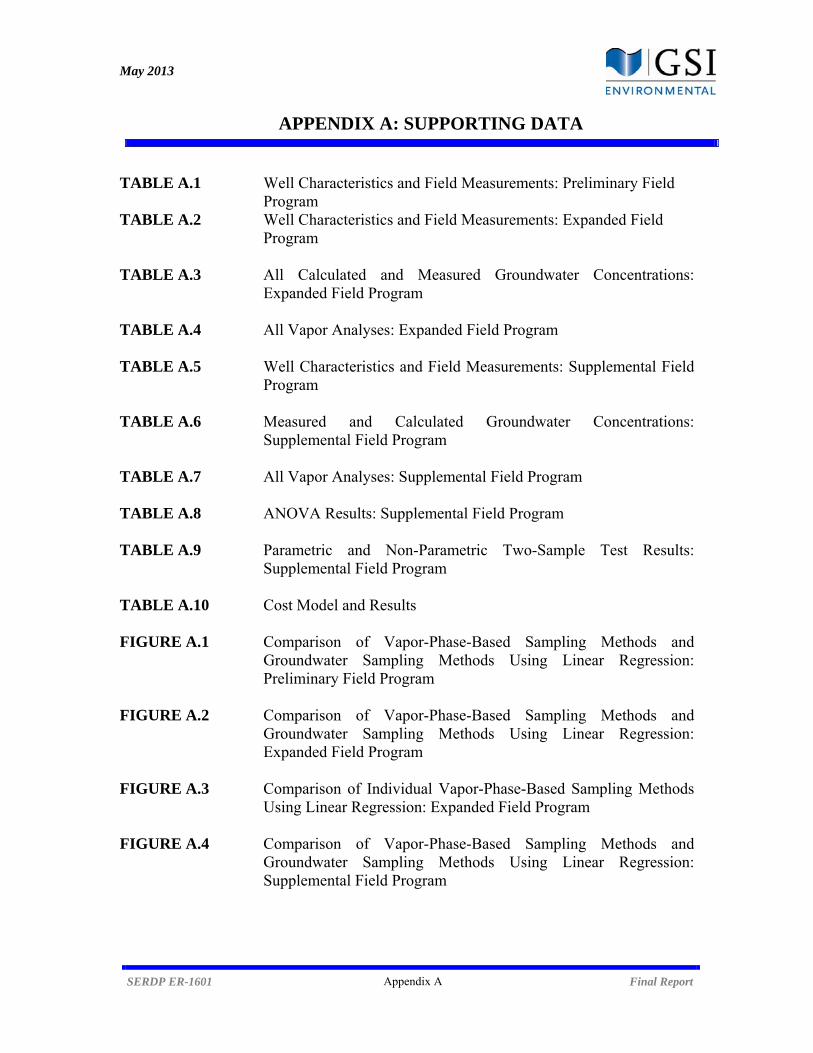
May 2013
SERDP ER-1601 Appendix A Final Report
APPENDIX A: SUPPORTING DATA
TABLE A.1 Well Characteristics and Field Measurements: Preliminary Field Program
TABLE A.2 Well Characteristics and Field Measurements: Expanded Field Program
TABLE A.3 All Calculated and Measured Groundwater Concentrations:
Expanded Field Program TABLE A.4 All Vapor Analyses: Expanded Field Program TABLE A.5 Well Characteristics and Field Measurements: Supplemental Field
Program TABLE A.6 Measured and Calculated Groundwater Concentrations:
Supplemental Field Program TABLE A.7 All Vapor Analyses: Supplemental Field Program TABLE A.8 ANOVA Results: Supplemental Field Program TABLE A.9 Parametric and Non-Parametric Two-Sample Test Results:
Supplemental Field Program TABLE A.10 Cost Model and Results FIGURE A.1 Comparison of Vapor-Phase-Based Sampling Methods and
Groundwater Sampling Methods Using Linear Regression: Preliminary Field Program
FIGURE A.2 Comparison of Vapor-Phase-Based Sampling Methods and
Groundwater Sampling Methods Using Linear Regression: Expanded Field Program
FIGURE A.3 Comparison of Individual Vapor-Phase-Based Sampling Methods
Using Linear Regression: Expanded Field Program FIGURE A.4 Comparison of Vapor-Phase-Based Sampling Methods and
Groundwater Sampling Methods Using Linear Regression: Supplemental Field Program
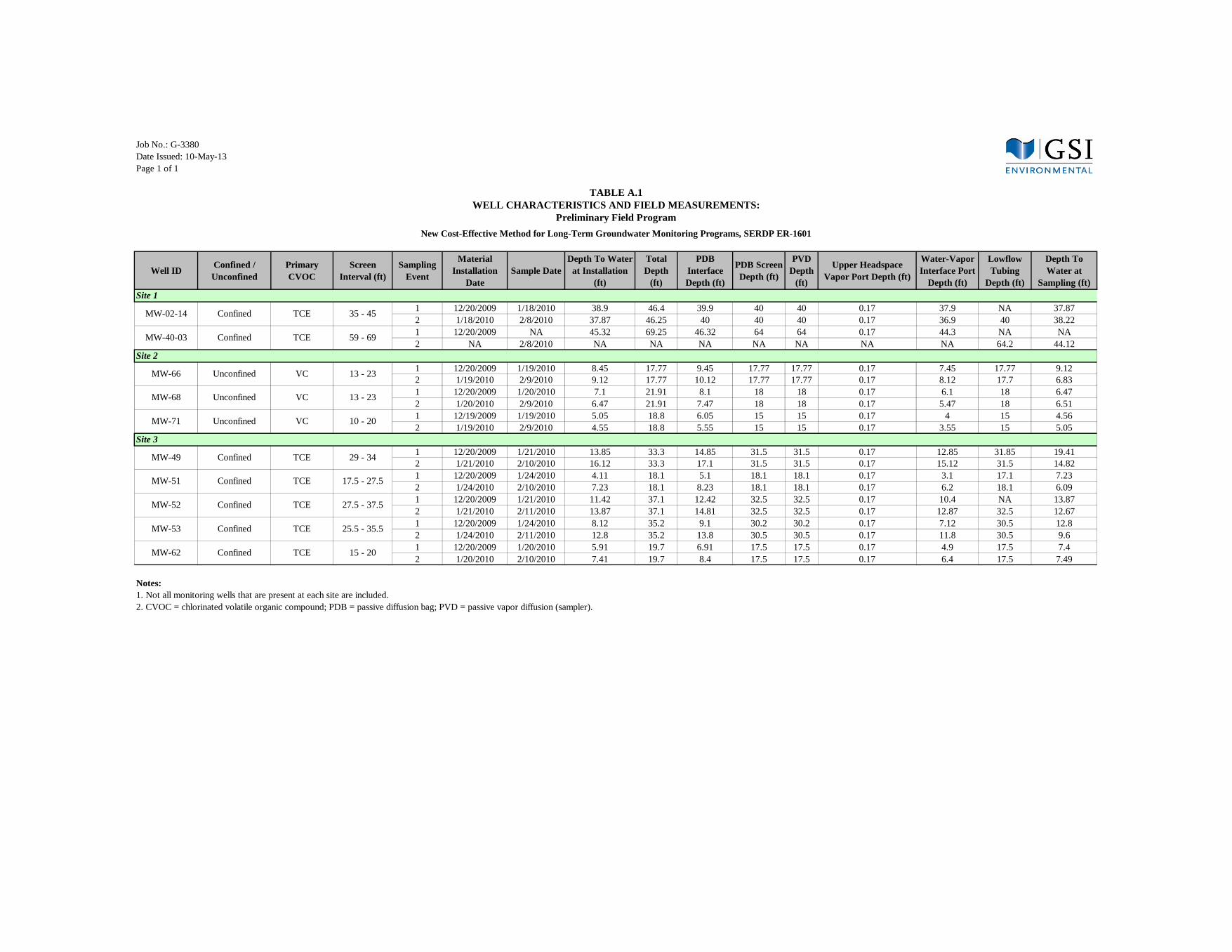
Job No.: G-3380Date Issued: 10-May-13Page 1 of 1
Well ID Confined / Unconfined
Primary CVOC
Screen Interval (ft)
Sampling Event
Material Installation
Date Sample Date
Depth To Water at Installation
(ft)
Total Depth
(ft)
PDB Interface Depth (ft)
PDB Screen Depth (ft)
PVD Depth
(ft)
Upper Headspace Vapor Port Depth (ft)
Water-Vapor Interface Port
Depth (ft)
Lowflow Tubing
Depth (ft)
Depth To Water at
Sampling (ft)
1 12/20/2009 1/18/2010 38.9 46.4 39.9 40 40 0.17 37.9 NA 37.872 1/18/2010 2/8/2010 37.87 46.25 40 40 40 0.17 36.9 40 38.221 12/20/2009 NA 45.32 69.25 46.32 64 64 0.17 44.3 NA NA2 NA 2/8/2010 NA NA NA NA NA NA NA 64.2 44.12
1 12/20/2009 1/19/2010 8.45 17.77 9.45 17.77 17.77 0.17 7.45 17.77 9.122 1/19/2010 2/9/2010 9.12 17.77 10.12 17.77 17.77 0.17 8.12 17.7 6.831 12/20/2009 1/20/2010 7.1 21.91 8.1 18 18 0.17 6.1 18 6.472 1/20/2010 2/9/2010 6.47 21.91 7.47 18 18 0.17 5.47 18 6.511 12/19/2009 1/19/2010 5.05 18.8 6.05 15 15 0.17 4 15 4.562 1/19/2010 2/9/2010 4.55 18.8 5.55 15 15 0.17 3.55 15 5.05
1 12/20/2009 1/21/2010 13.85 33.3 14.85 31.5 31.5 0.17 12.85 31.85 19.412 1/21/2010 2/10/2010 16.12 33.3 17.1 31.5 31.5 0.17 15.12 31.5 14.821 12/20/2009 1/24/2010 4.11 18.1 5.1 18.1 18.1 0.17 3.1 17.1 7.232 1/24/2010 2/10/2010 7.23 18.1 8.23 18.1 18.1 0.17 6.2 18.1 6.091 12/20/2009 1/21/2010 11.42 37.1 12.42 32.5 32.5 0.17 10.4 NA 13.872 1/21/2010 2/11/2010 13.87 37.1 14.81 32.5 32.5 0.17 12.87 32.5 12.671 12/20/2009 1/24/2010 8.12 35.2 9.1 30.2 30.2 0.17 7.12 30.5 12.82 1/24/2010 2/11/2010 12.8 35.2 13.8 30.5 30.5 0.17 11.8 30.5 9.61 12/20/2009 1/20/2010 5.91 19.7 6.91 17.5 17.5 0.17 4.9 17.5 7.42 1/20/2010 2/10/2010 7.41 19.7 8.4 17.5 17.5 0.17 6.4 17.5 7.49
Notes:1. Not all monitoring wells that are present at each site are included.2. CVOC = chlorinated volatile organic compound; PDB = passive diffusion bag; PVD = passive vapor diffusion (sampler).
Unconfined 13 - 23
MW-66
35 - 45
MW-40-03 Confined 59 - 69
MW-02-14 Confined TCE
TCE
MW-62 Confined 15 - 20
TCE
TCE
MW-53 Confined 25.5 - 35.5
TCE
17.5 - 27.5
MW-52 Confined 27.5 - 37.5
TCE
TCE
MW-49 Confined 29 - 34
MW-51 Confined
Site 1
Site 2
Site 3
TABLE A.1WELL CHARACTERISTICS AND FIELD MEASUREMENTS:
Preliminary Field ProgramNew Cost-Effective Method for Long-Term Groundwater Monitoring Programs, SERDP ER-1601
Unconfined
MW-71 10 - 20
VC
VC
VCUnconfined
13 - 23
MW-68
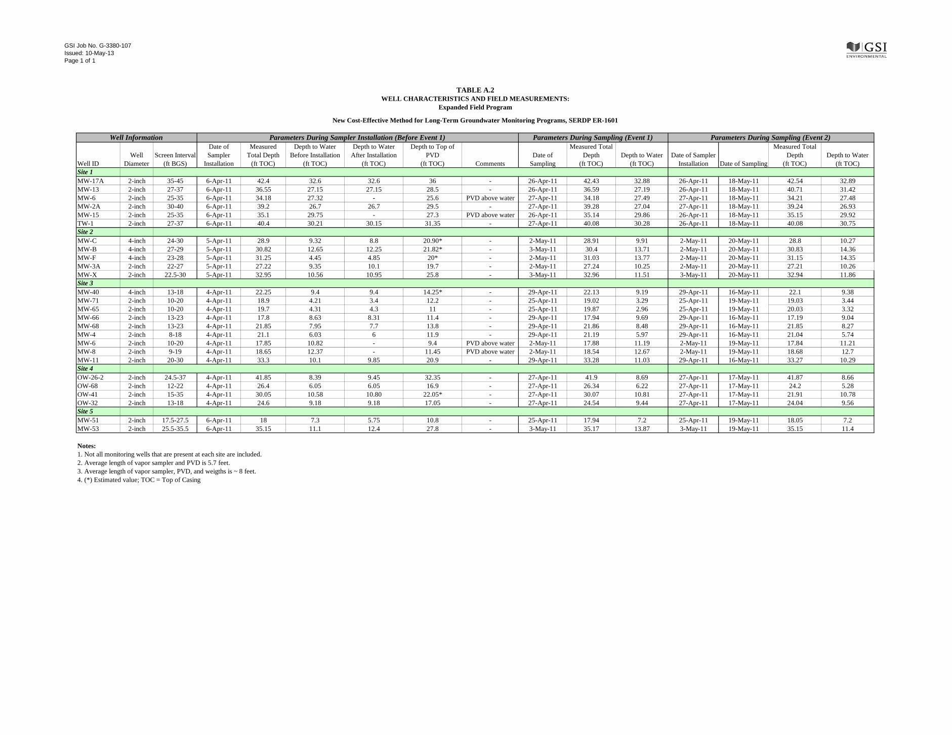
GSI Job No. G-3380-107Issued: 10-May-13Page 1 of 1
Well IDWell
DiameterScreen Interval
(ft BGS)
Date of Sampler
Installation
Measured Total Depth
(ft TOC)
Depth to Water Before Installation
(ft TOC)
Depth to Water After Installation
(ft TOC)
Depth to Top of PVD
(ft TOC) CommentsDate of
Sampling
Measured Total Depth
(ft TOC)Depth to Water
(ft TOC)Date of Sampler
Installation Date of Sampling
Measured Total Depth
(ft TOC)Depth to Water
(ft TOC)Site 1MW-17A 2-inch 35-45 6-Apr-11 42.4 32.6 32.6 36 - 26-Apr-11 42.43 32.88 26-Apr-11 18-May-11 42.54 32.89MW-13 2-inch 27-37 6-Apr-11 36.55 27.15 27.15 28.5 - 26-Apr-11 36.59 27.19 26-Apr-11 18-May-11 40.71 31.42MW-6 2-inch 25-35 6-Apr-11 34.18 27.32 - 25.6 PVD above water 27-Apr-11 34.18 27.49 27-Apr-11 18-May-11 34.21 27.48MW-2A 2-inch 30-40 6-Apr-11 39.2 26.7 26.7 29.5 - 27-Apr-11 39.28 27.04 27-Apr-11 18-May-11 39.24 26.93MW-15 2-inch 25-35 6-Apr-11 35.1 29.75 - 27.3 PVD above water 26-Apr-11 35.14 29.86 26-Apr-11 18-May-11 35.15 29.92TW-1 2-inch 27-37 6-Apr-11 40.4 30.21 30.15 31.35 - 27-Apr-11 40.08 30.28 26-Apr-11 18-May-11 40.08 30.75Site 2MW-C 4-inch 24-30 5-Apr-11 28.9 9.32 8.8 20.90* - 2-May-11 28.91 9.91 2-May-11 20-May-11 28.8 10.27MW-B 4-inch 27-29 5-Apr-11 30.82 12.65 12.25 21.82* - 3-May-11 30.4 13.71 2-May-11 20-May-11 30.83 14.36MW-F 4-inch 23-28 5-Apr-11 31.25 4.45 4.85 20* - 2-May-11 31.03 13.77 2-May-11 20-May-11 31.15 14.35MW-3A 2-inch 22-27 5-Apr-11 27.22 9.35 10.1 19.7 - 2-May-11 27.24 10.25 2-May-11 20-May-11 27.21 10.26MW-X 2-inch 22.5-30 5-Apr-11 32.95 10.56 10.95 25.8 - 3-May-11 32.96 11.51 3-May-11 20-May-11 32.94 11.86Site 3MW-40 4-inch 13-18 4-Apr-11 22.25 9.4 9.4 14.25* - 29-Apr-11 22.13 9.19 29-Apr-11 16-May-11 22.1 9.38MW-71 2-inch 10-20 4-Apr-11 18.9 4.21 3.4 12.2 - 25-Apr-11 19.02 3.29 25-Apr-11 19-May-11 19.03 3.44MW-65 2-inch 10-20 4-Apr-11 19.7 4.31 4.3 11 - 25-Apr-11 19.87 2.96 25-Apr-11 19-May-11 20.03 3.32MW-66 2-inch 13-23 4-Apr-11 17.8 8.63 8.31 11.4 - 29-Apr-11 17.94 9.69 29-Apr-11 16-May-11 17.19 9.04MW-68 2-inch 13-23 4-Apr-11 21.85 7.95 7.7 13.8 - 29-Apr-11 21.86 8.48 29-Apr-11 16-May-11 21.85 8.27MW-4 2-inch 8-18 4-Apr-11 21.1 6.03 6 11.9 - 29-Apr-11 21.19 5.97 29-Apr-11 16-May-11 21.04 5.74MW-6 2-inch 10-20 4-Apr-11 17.85 10.82 - 9.4 PVD above water 2-May-11 17.88 11.19 2-May-11 19-May-11 17.84 11.21MW-8 2-inch 9-19 4-Apr-11 18.65 12.37 - 11.45 PVD above water 2-May-11 18.54 12.67 2-May-11 19-May-11 18.68 12.7MW-11 2-inch 20-30 4-Apr-11 33.3 10.1 9.85 20.9 - 29-Apr-11 33.28 11.03 29-Apr-11 16-May-11 33.27 10.29Site 4OW-26-2 2-inch 24.5-37 4-Apr-11 41.85 8.39 9.45 32.35 - 27-Apr-11 41.9 8.69 27-Apr-11 17-May-11 41.87 8.66OW-68 2-inch 12-22 4-Apr-11 26.4 6.05 6.05 16.9 - 27-Apr-11 26.34 6.22 27-Apr-11 17-May-11 24.2 5.28OW-41 2-inch 15-35 4-Apr-11 30.05 10.58 10.80 22.05* - 27-Apr-11 30.07 10.81 27-Apr-11 17-May-11 21.91 10.78OW-32 2-inch 13-18 4-Apr-11 24.6 9.18 9.18 17.05 - 27-Apr-11 24.54 9.44 27-Apr-11 17-May-11 24.04 9.56Site 5MW-51 2-inch 17.5-27.5 6-Apr-11 18 7.3 5.75 10.8 - 25-Apr-11 17.94 7.2 25-Apr-11 19-May-11 18.05 7.2MW-53 2-inch 25.5-35.5 6-Apr-11 35.15 11.1 12.4 27.8 - 3-May-11 35.17 13.87 3-May-11 19-May-11 35.15 11.4
Notes:1. Not all monitoring wells that are present at each site are included.2. Average length of vapor sampler and PVD is 5.7 feet.3. Average length of vapor sampler, PVD, and weigths is ~ 8 feet.4. (*) Estimated value; TOC = Top of Casing
TABLE A.2WELL CHARACTERISTICS AND FIELD MEASUREMENTS:
New Cost-Effective Method for Long-Term Groundwater Monitoring Programs, SERDP ER-1601
Parameters During Sampling (Event 2)Parameters During Sampling (Event 1)Well Information Parameters During Sampler Installation (Before Event 1)
Expanded Field Program

GSI Job No. G-3380-107Issued: 10-May-13
ug/L log (ug/L) ug/L
Pressure Corrected
(ug/L) log (ug/L) RPD ABS RPD ug/L
Pressure Corrected
(ug/L) log (ug/L) RPD ABS RPD ug/L
Pressure Corrected
(ug/L) log (ug/L) RPD ABS RPDSITE 1 MW-17A 1 35 33 2.4 4.8 0.9 75.9 3 6 <2 - - 0.033 0.039 -1.41
Dup 1 35 33 2.4 4.8 0.9 75.9 3 6 <22 35 32.6 2.4 2.6 4.7 74.0 4.36 5.61 <1
Dup 2 35 32.6 2.4 2.6 4.7 74.0 4.36 5.61 <1SITE 1 MW-13 1 27 27.15 -0.1 1.7 3.5 75.6 1.31 3.81 <2 - -
2 27 27.15 -0.1 2.2 2.4 74.7 0 1 1.1 0.04SITE 1 MW-6 1 25 27.32 -2.3 5.8 0.5 77.4 0 0.61 6.5 0.81 1.3 1.3 0.11 134% 134% 1.667 1.697 0.23 117% 117%
2 25 27.32 -2.3 2.8 3.7 74.2 0 0.42 9.1 0.96SITE 1 MW-2A 1 30 26.7 3.3 2.1 1.1 78.9 1.46 3.96 3.7 0.57 8.744 9.764 0.99 -90% 90% 6.971 7.784 0.89 -71% 71%
2 30 26.7 3.3 2.6 0.5 76.9 3.82 5.07 2.2 0.34SITE 1 MW-15 1 25 29.75 -4.8 2.7 2.3 75.3 0 2.5 <2 - - 0.045 0.049 -1.31
2 25 29.75 -4.8 4.3 2.2 73.0 0 0.7 <1SITE 1 TW-1 1 27 30.21 -3.2 3.9 1.6 77.7 1.07 3.57 <2 - - 0.071 0.079 -1.10
2 27 30.21 -3.2 4.2 3.6 75.6 1.85 3.1 <1SITE 2 MW-C 1 24 8.8 15.2 0.8 1.2 77.7 10 12.5 0.74 -0.13 7.669 10.492 1.02 -174% 174% 2.311 3.163 0.50 -124% 124%
2 24 8.8 15.2 1.5 2.2 78.6 11.88 13.13 <0.85SITE 2 MW-B 1 27 12.25 14.8 0.9 2.6 70.5 8.1 10.6 46 1.66 0.297 0.389 -0.41 197% 197%
2 27 12.25 14.8 1.8 2.2 72.7 8.71 9.96 27 1.43SITE 2 MW-F 1 23 4.85 18.2 0.4 3.3 73.0 6.23 8.73 <0.11 8.373 10.526 1.02 - - 7.102 8.928 0.95
2 23 4.85 18.2 2.6 4.5 71.4 6.9 8.15 <0.85SITE 2 MW-3A 1 22 10.1 11.9 1.0 0.3 76.9 9.55 12.45 1500 3.18 1756.310 2400.377 3.38 -46% 46% 51.1 69.8 1.84 182% 182% 0.279 0.381 -0.42 200% 200%
2 22 10.1 11.9 1.8 3.8 76.5 10.69 11.94 1400 3.15SITE 2 MW-X 1 22.5 10.95 11.6 3.4 -0.1 74.4 14.29 16.79 0.99 0.00 0.18 0.27 -0.57 114% 114%
2 22.5 10.95 11.6 1.3 1.6 72.8 15.19 16.44 3.4 0.53SITE 3 MW-40 1 13 9.4 3.6 1.1 1.4 73.7 5.06 7.56 15000 4.18 18737.524 22910.003 4.36 -42% 42% 3071.482 3755.441 3.57 120% 120%
2 13 9.4 3.6 0.1 1.5 72.0 6.12 7.37 16000 4.20SITE 3 MW-71 1 10 3.4 6.6 1.0 1.5 74.4 8.91 11.41 53000 4.72 105921.653 141520.064 5.15 -91% 91% 6592 8807 3.94 143% 143%
2 10 3.4 6.6 0.3 0.9 73.4 10.01 11.26 22000 4.34SITE 3 MW-65 1 10 4.3 5.7 0.6 1.9 75.3 8.04 10.54 310000 5.49 359931.970 471675.210 5.67 -41% 41% 26216 34355 4.54 160% 160%
2 10 4.3 5.7 0.6 2.1 71.5 8.93 10.18 200000 5.30SITE 3 MW-66 1 13 8.31 4.7 0.9 7.8 72.7 1.71 4.21 85000 4.93 105211.352 118258.179 5.07 -33% 33% 14159 15915 4.20 137% 137%
2 13 8.31 4.7 0.4 0.5 72.5 3.61 4.86 47000 4.67SITE 3 MW-68 1 13 7.7 5.3 0.8 1.9 72.5 5.32 7.82 13000 4.11 33164.516 40803.589 4.61 -103% 103% 2186.1 2689.6 3.43 131% 131% 6368.202 7835.045 3.89 50% 50%
2 13 7.7 5.3 0.6 0.5 72.4 6.78 8.03 14000 4.15SITE 3 MW-4 1 8 6 2.0 1.0 2.2 73.7 5.93 8.43 320000 5.51 658109.794 821522.623 5.91 -88% 88% 19420 24242 4.38 172% 172%
2 8 6 2.0 0.4 0.7 73.3 7.41 8.66 220000 5.34SITE 3 MW-6 1 10 10.82 -0.8 0.9 2.1 71.5 0 2.2 21000 4.32 21793.827 23206.093 4.37 -10% 10% 3691.6 3930.9 3.59 137% 137%
2 10 10.82 -0.8 0.6 0.9 71.5 0 1 13000 4.11SITE 3 MW-8 1 9 12.37 -3.4 1.2 1.6 70.8 0 1.9 5100 3.71 15478.980 16345.256 4.21 -105% 105% 1136 1200 3.08 124% 124%
2 9 12.37 -3.4 0.0 1.1 71.6 0 1.25 3100 3.49SITE 3 MW-11 1 20 9.85 10.2 1.4 2.2 72.9 9.87 12.37 31000 4.49
2 20 9.85 10.2 1.1 0.5 71.8 11.86 13.11 42000 4.62Dup 2 20 9.85 10.2 1.1 0.5 71.8 11.86 13.11 35000 4.54
SITE 4 OW-26-2 1 24.5 9.45 15.1 1.3 3.6 76.9 23.66 26.16 12000 4.08 159.497 282.397 2.45 191% 191% 22 40 1.60 199% 199% 102.391 181.287 2.26 194% 194%Dup 1 24.5 9.45 15.1 1.3 3.6 76.9 23.66 26.16 8800 3.94 159.497 282.397 2.45 188% 188%
2 24.5 9.45 15.1 1.4 2.7 76.9 24.94 26.19 9800 3.99SITE 4 OW-68 1 12 6.05 6.0 1.9 1.7 77.6 10.68 13.18 7 0.85 56.065 77.830 1.89 -167% 167% 0.2 0.3 -0.50 183% 183% 0.247 0.343 -0.46 181% 181%
2 12 6.05 6.0 1.1 0.9 76.3 12.87 14.12 9.9 1.00SITE 4 OW-41 1 15 10.8 4.2 1.3 3.6 76.3 11.24 13.74 2400 3.38
2 15 10.8 4.2 1.1 2.2 73.7 12.52 13.77 2400 3.38SITE 4 OW-32 1 13 9.18 3.8 1.2 2.7 73.7 7.61 10.11 69 1.84 25.939 33.664 1.53 69% 69% 2212 2870 3.46 -191% 191% 7.899 10.252 1.01 148% 148%
2 13 9.18 3.8 0.9 1.2 73.4 8.74 9.99 220 2.34Dup 2 13 9.18 3.8 0.9 1.2 73.4 8.74 9.99 170 2.23
SITE 5 MW-51 1 17.5 5.75 11.8 1.7 0.9 74.8 3.6 6.1 <0.11 0.058 0.068 -1.17Dup 1 17.5 5.75 11.8 1.7 0.9 74.8 3.6 6.1 <0.11
2 17.5 5.75 11.8 1.3 2.0 71.7 4.85 6.1 <0.85SITE 5 MW-53 1 25.5 12.4 13.1 1.6 2.9 71.1 13.93 16.43 44 1.64 1.9 2.8 0.45 176% 176% 0.020 0.030 -1.52 200% 200%
2 25.5 12.4 13.1 1.4 3.1 73.4 17.65 18.9 <42
Expanded Field ProgramALL CALCULATED AND MEASURED GROUNDWATER CONCENTRATIONS:
TABLE A.3
New Cost-Effective Method for Long-Term Groundwater Monitoring Programs, SERDP ER-1601
Groundwater Concentration - Measured or Calculated (ug/L)
Change in Dissolved
Oxygen during purging (mg/L)
Constituent
HAPSITEGW
Temperature
Field PIDThickness of Water
Column above short PVD
VC
Sample Type
Thickness of Water Column above Longer
PVDs
Dissolved Oxygen (after
purging) (mg/L)
Site ID Well ID Sampling Date
Low-Flow GSI Extended Length PVD
Distance to Top of
Screen (ft)
Depth to Water (ft)
Distance from Depth of
Water to Top of Well Screen
(ft)
Laboratory Field GC

GSI Job No. G-3380-107Issued: 10-May-13
ug/L log (ug/L) ug/L
Pressure Corrected
(ug/L) log (ug/L) RPD ABS RPD ug/L
Pressure Corrected
(ug/L) log (ug/L) RPD ABS RPD ug/L
Pressure Corrected
(ug/L) log (ug/L) RPD ABS RPD
Expanded Field ProgramALL CALCULATED AND MEASURED GROUNDWATER CONCENTRATIONS:
TABLE A.3
New Cost-Effective Method for Long-Term Groundwater Monitoring Programs, SERDP ER-1601
Groundwater Concentration - Measured or Calculated (ug/L)
Change in Dissolved
Oxygen during purging (mg/L)
Constituent
HAPSITEGW
Temperature
Field PIDThickness of Water
Column above short PVD
Sample Type
Thickness of Water Column above Longer
PVDs
Dissolved Oxygen (after
purging) (mg/L)
Site ID Well ID Sampling Date
Low-Flow GSI Extended Length PVD
Distance to Top of
Screen (ft)
Depth to Water (ft)
Distance from Depth of
Water to Top of Well Screen
(ft)
Laboratory Field GC
SITE 1 MW-17A 1 35 33 2 4.8 0.9 75.9 3 6 4 0.60 4.4 5.1 0.71 -24% 24% 0.870 1.014 0.01 119% 119%Dup 1 35 33 2 4.8 0.9 75.9 3 6 4.2 0.62
2 35 32.6 2 2.6 4.7 74.0 4.36 5.61 4.2 0.62Dup 2 35 32.6 2 2.6 4.7 74.0 4.36 5.61 4.1 0.61
SITE 1 MW-13 1 27 27.15 0 1.7 3.5 75.6 1.31 3.81 31.5 1.50 10.530 11.712 1.07 92% 92% 7.0 7.7 0.89 121% 121%2 27 27.15 0 2.2 2.4 74.7 0 1 42.5 1.63
SITE 1 MW-6 1 25 27.32 -2 5.8 0.5 77.4 0 0.61 7.1 0.85 8.280 8.429 0.93 -17% 17% 13.3 13.6 1.13 -63% 63% 6.265 6.378 0.80 11% 11%2 25 27.32 -2 2.8 3.7 74.2 0 0.42 10.3 1.01
SITE 1 MW-2A 1 30 26.7 3 2.1 1.1 78.9 1.46 3.96 1.6 0.20 1.260 1.407 0.15 13% 13%2 30 26.7 3 2.6 0.5 76.9 3.82 5.07 1.9 0.28
SITE 1 MW-15 1 25 29.75 -5 2.7 2.3 75.3 0 2.5 2.6 0.41 0.624 0.670 -0.17 118% 118% 1.081 1.160 0.06 77% 77%2 25 29.75 -5 4.3 2.2 73.0 0 0.7 3 0.48
SITE 1 TW-1 1 27 30.21 -3 3.9 1.6 77.7 1.07 3.57 8.8 0.94 24.669 27.263 1.44 -102% 102% 19.03 21.03 1.32 -82% 82% 2.933 3.242 0.51 92% 92%2 27 30.21 -3 4.2 3.6 75.6 1.85 3.1 11.8 1.07
SITE 2 MW-C 1 24 8.8 15 0.8 1.2 77.7 10 12.5 <0.18 0.274 0.375 -0.432 24 8.8 15 1.5 2.2 78.6 11.88 13.13 <1.6
SITE 2 MW-B 1 27 12.25 15 0.9 2.6 70.5 8.1 10.6 2.8 0.45 1.651 2.167 0.34 25% 25%2 27 12.25 15 1.8 2.2 72.7 8.71 9.96 6.8 0.83
SITE 2 MW-F 1 23 4.85 18 0.4 3.3 73.0 6.23 8.73 <0.18 - - 0.923 1.160 0.062 23 4.85 18 2.6 4.5 71.4 6.9 8.15 <1.6
SITE 2 MW-3A 1 22 10.1 12 1.0 0.3 76.9 9.55 12.45 280 2.45 92.3 126.2 2.10 76% 76% 0.024 0.033 -1.48 200% 200%2 22 10.1 12 1.8 3.8 76.5 10.69 11.94 160 2.20
SITE 2 MW-X 1 22.5 10.95 12 3.4 -0.1 74.4 14.29 16.79 30 1.48 54.52 81.48 1.91 -92% 92% 17.712 26.472 1.42 12% 12%2 22.5 10.95 12 1.3 1.6 72.8 15.19 16.44 54 1.73
SITE 3 MW-40 1 13 9.4 4 1.1 1.4 73.7 5.06 7.56 <92 13 9.4 4 0.1 1.5 72.0 6.12 7.37 <32
SITE 3 MW-71 1 10 3.4 7 1.0 1.5 74.4 8.91 11.41 110 2.04 136 182 2.26 -49% 49%2 10 3.4 7 0.3 0.9 73.4 10.01 11.26 39
SITE 3 MW-65 1 10 4.3 6 0.6 1.9 75.3 8.04 10.54 660 2.82 549 720 2.86 -9% 9%2 10 4.3 6 0.6 2.1 71.5 8.93 10.18 740 2.87
SITE 3 MW-66 1 13 8.31 5 0.9 7.8 72.7 1.71 4.21 1300 3.11 2133 2398 3.38 -59% 59%2 13 8.31 5 0.4 0.5 72.5 3.61 4.86 1300 3.11
SITE 3 MW-68 1 13 7.7 5 0.8 1.9 72.5 5.32 7.82 <9 - - 12.746 15.682 1.202 13 7.7 5 0.6 0.5 72.4 6.78 8.03 <32
SITE 3 MW-4 1 8 6 2 1.0 2.2 73.7 5.93 8.43 1700 3.23 1027 1282 3.11 28% 28%2 8 6 2 0.4 0.7 73.3 7.41 8.66 1600 3.20
SITE 3 MW-6 1 10 10.82 -1 0.9 2.1 71.5 0 2.2 21 1.32 37.6 40.0 1.60 -62% 62%2 10 10.82 -1 0.6 0.9 71.5 0 1 <79
SITE 3 MW-8 1 9 12.37 -3 1.2 1.6 70.8 0 1.9 17 1.23 39 41 1.61 -82% 82%2 9 12.37 -3 0.0 1.1 71.6 0 1.25 <32
SITE 3 MW-11 1 20 9.85 10 1.4 2.2 72.9 9.87 12.37 780 2.892 20 9.85 10 1.1 0.5 71.8 11.86 13.11 1000 3.00
Dup 2 20 9.85 10 1.1 0.5 71.8 11.86 13.11 1000 3.00SITE 4 OW-26-2 1 24.5 9.45 15 1.3 3.6 76.9 23.66 26.16 <18 - - 0.313 0.554 -0.26
Dup 24.5 9.45 15 1.3 3.6 76.9 23.66 26.16 <182 24.5 9.45 15 1.4 2.7 76.9 24.94 26.19 81 1.91
SITE 4 OW-68 1 12 6.05 6 1.9 1.7 77.6 10.68 13.18 <3.6 - -2 12 6.05 6 1.1 0.9 76.3 12.87 14.12 <1.6
SITE 4 OW-41 1 15 10.8 4 1.3 3.6 76.3 11.24 13.74 150 2.182 15 10.8 4 1.1 2.2 73.7 12.52 13.77 200 2.30
SITE 4 OW-32 1 13 9.18 4 1.2 2.7 73.7 7.61 10.11 0.84 -0.08 267 346 2.54 -199% 199% 0.233 0.303 -0.52 94% 94%2 13 9.18 4 0.9 1.2 73.4 8.74 9.99 <1.6
Dup 2 13 9.18 4 0.9 1.2 73.4 8.74 9.99 <1.6SITE 5 MW-51 1 17.5 5.75 12 1.7 0.9 74.8 3.6 6.1 28 1.45 12.594 14.856 1.17 61% 61% 6.314 7.449 0.87 116% 116%
Dup 1 17.5 5.75 12 1.7 0.9 74.8 3.6 6.1 28 1.45 6.314 7.449 0.87 116% 116%2 17.5 5.75 12 1.3 2.0 71.7 4.85 6.1 40 1.60
SITE 5 MW-53 1 25.5 12.4 13 1.6 2.9 71.1 13.93 16.43 11000 4.04 3242.539 4811.756 3.68 78% 78% 4910.2 7286.4 3.86 41% 41% 6.446 9.565 0.98 200% 200%2 25.5 12.4 13 1.4 3.1 73.4 17.65 18.9 11000 4.04
TCE
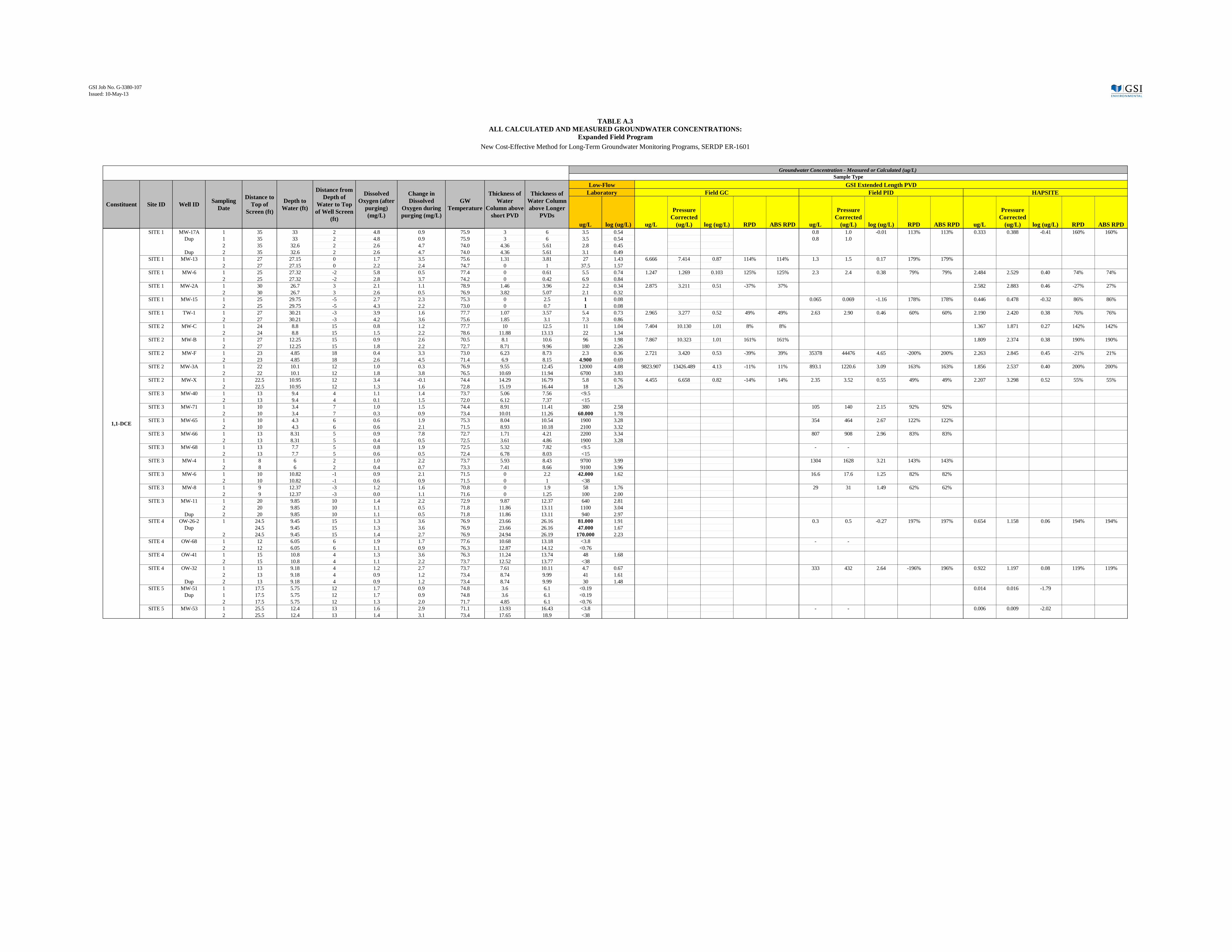
GSI Job No. G-3380-107Issued: 10-May-13
ug/L log (ug/L) ug/L
Pressure Corrected
(ug/L) log (ug/L) RPD ABS RPD ug/L
Pressure Corrected
(ug/L) log (ug/L) RPD ABS RPD ug/L
Pressure Corrected
(ug/L) log (ug/L) RPD ABS RPD
Expanded Field ProgramALL CALCULATED AND MEASURED GROUNDWATER CONCENTRATIONS:
TABLE A.3
New Cost-Effective Method for Long-Term Groundwater Monitoring Programs, SERDP ER-1601
Groundwater Concentration - Measured or Calculated (ug/L)
Change in Dissolved
Oxygen during purging (mg/L)
Constituent
HAPSITEGW
Temperature
Field PIDThickness of Water
Column above short PVD
Sample Type
Thickness of Water Column above Longer
PVDs
Dissolved Oxygen (after
purging) (mg/L)
Site ID Well ID Sampling Date
Low-Flow GSI Extended Length PVD
Distance to Top of
Screen (ft)
Depth to Water (ft)
Distance from Depth of
Water to Top of Well Screen
(ft)
Laboratory Field GC
SITE 1 MW-17A 1 35 33 2 4.8 0.9 75.9 3 6 3.5 0.54 0.8 1.0 -0.01 113% 113% 0.333 0.388 -0.41 160% 160%Dup 1 35 33 2 4.8 0.9 75.9 3 6 3.5 0.54 0.8 1.0
2 35 32.6 2 2.6 4.7 74.0 4.36 5.61 2.8 0.45Dup 2 35 32.6 2 2.6 4.7 74.0 4.36 5.61 3.1 0.49
SITE 1 MW-13 1 27 27.15 0 1.7 3.5 75.6 1.31 3.81 27 1.43 6.666 7.414 0.87 114% 114% 1.3 1.5 0.17 179% 179%2 27 27.15 0 2.2 2.4 74.7 0 1 37.5 1.57
SITE 1 MW-6 1 25 27.32 -2 5.8 0.5 77.4 0 0.61 5.5 0.74 1.247 1.269 0.103 125% 125% 2.3 2.4 0.38 79% 79% 2.484 2.529 0.40 74% 74%2 25 27.32 -2 2.8 3.7 74.2 0 0.42 6.9 0.84
SITE 1 MW-2A 1 30 26.7 3 2.1 1.1 78.9 1.46 3.96 2.2 0.34 2.875 3.211 0.51 -37% 37% 2.582 2.883 0.46 -27% 27%2 30 26.7 3 2.6 0.5 76.9 3.82 5.07 2.1 0.32
SITE 1 MW-15 1 25 29.75 -5 2.7 2.3 75.3 0 2.5 1 0.08 0.065 0.069 -1.16 178% 178% 0.446 0.478 -0.32 86% 86%2 25 29.75 -5 4.3 2.2 73.0 0 0.7 1 0.08
SITE 1 TW-1 1 27 30.21 -3 3.9 1.6 77.7 1.07 3.57 5.4 0.73 2.965 3.277 0.52 49% 49% 2.63 2.90 0.46 60% 60% 2.190 2.420 0.38 76% 76%2 27 30.21 -3 4.2 3.6 75.6 1.85 3.1 7.3 0.86
SITE 2 MW-C 1 24 8.8 15 0.8 1.2 77.7 10 12.5 11 1.04 7.404 10.130 1.01 8% 8% 1.367 1.871 0.27 142% 142%2 24 8.8 15 1.5 2.2 78.6 11.88 13.13 22 1.34
SITE 2 MW-B 1 27 12.25 15 0.9 2.6 70.5 8.1 10.6 96 1.98 7.867 10.323 1.01 161% 161% 1.809 2.374 0.38 190% 190%2 27 12.25 15 1.8 2.2 72.7 8.71 9.96 180 2.26
SITE 2 MW-F 1 23 4.85 18 0.4 3.3 73.0 6.23 8.73 2.3 0.36 2.721 3.420 0.53 -39% 39% 35378 44476 4.65 -200% 200% 2.263 2.845 0.45 -21% 21%2 23 4.85 18 2.6 4.5 71.4 6.9 8.15 4.900 0.69
SITE 2 MW-3A 1 22 10.1 12 1.0 0.3 76.9 9.55 12.45 12000 4.08 9823.907 13426.489 4.13 -11% 11% 893.1 1220.6 3.09 163% 163% 1.856 2.537 0.40 200% 200%2 22 10.1 12 1.8 3.8 76.5 10.69 11.94 6700 3.83
SITE 2 MW-X 1 22.5 10.95 12 3.4 -0.1 74.4 14.29 16.79 5.8 0.76 4.455 6.658 0.82 -14% 14% 2.35 3.52 0.55 49% 49% 2.207 3.298 0.52 55% 55%2 22.5 10.95 12 1.3 1.6 72.8 15.19 16.44 18 1.26
SITE 3 MW-40 1 13 9.4 4 1.1 1.4 73.7 5.06 7.56 <9.52 13 9.4 4 0.1 1.5 72.0 6.12 7.37 <15
SITE 3 MW-71 1 10 3.4 7 1.0 1.5 74.4 8.91 11.41 380 2.58 105 140 2.15 92% 92%2 10 3.4 7 0.3 0.9 73.4 10.01 11.26 60.000 1.78
SITE 3 MW-65 1 10 4.3 6 0.6 1.9 75.3 8.04 10.54 1900 3.28 354 464 2.67 122% 122%2 10 4.3 6 0.6 2.1 71.5 8.93 10.18 2100 3.32
SITE 3 MW-66 1 13 8.31 5 0.9 7.8 72.7 1.71 4.21 2200 3.34 807 908 2.96 83% 83%2 13 8.31 5 0.4 0.5 72.5 3.61 4.86 1900 3.28
SITE 3 MW-68 1 13 7.7 5 0.8 1.9 72.5 5.32 7.82 <9.5 - -2 13 7.7 5 0.6 0.5 72.4 6.78 8.03 <15
SITE 3 MW-4 1 8 6 2 1.0 2.2 73.7 5.93 8.43 9700 3.99 1304 1628 3.21 143% 143%2 8 6 2 0.4 0.7 73.3 7.41 8.66 9100 3.96
SITE 3 MW-6 1 10 10.82 -1 0.9 2.1 71.5 0 2.2 42.000 1.62 16.6 17.6 1.25 82% 82%2 10 10.82 -1 0.6 0.9 71.5 0 1 <38
SITE 3 MW-8 1 9 12.37 -3 1.2 1.6 70.8 0 1.9 58 1.76 29 31 1.49 62% 62%2 9 12.37 -3 0.0 1.1 71.6 0 1.25 100 2.00
SITE 3 MW-11 1 20 9.85 10 1.4 2.2 72.9 9.87 12.37 640 2.812 20 9.85 10 1.1 0.5 71.8 11.86 13.11 1100 3.04
Dup 2 20 9.85 10 1.1 0.5 71.8 11.86 13.11 940 2.97SITE 4 OW-26-2 1 24.5 9.45 15 1.3 3.6 76.9 23.66 26.16 81.000 1.91 0.3 0.5 -0.27 197% 197% 0.654 1.158 0.06 194% 194%
Dup 24.5 9.45 15 1.3 3.6 76.9 23.66 26.16 47.000 1.672 24.5 9.45 15 1.4 2.7 76.9 24.94 26.19 170.000 2.23
SITE 4 OW-68 1 12 6.05 6 1.9 1.7 77.6 10.68 13.18 <3.8 - -2 12 6.05 6 1.1 0.9 76.3 12.87 14.12 <0.76
SITE 4 OW-41 1 15 10.8 4 1.3 3.6 76.3 11.24 13.74 48 1.682 15 10.8 4 1.1 2.2 73.7 12.52 13.77 <38
SITE 4 OW-32 1 13 9.18 4 1.2 2.7 73.7 7.61 10.11 4.7 0.67 333 432 2.64 -196% 196% 0.922 1.197 0.08 119% 119%2 13 9.18 4 0.9 1.2 73.4 8.74 9.99 41 1.61
Dup 2 13 9.18 4 0.9 1.2 73.4 8.74 9.99 30 1.48SITE 5 MW-51 1 17.5 5.75 12 1.7 0.9 74.8 3.6 6.1 <0.19 0.014 0.016 -1.79
Dup 1 17.5 5.75 12 1.7 0.9 74.8 3.6 6.1 <0.192 17.5 5.75 12 1.3 2.0 71.7 4.85 6.1 <0.76
SITE 5 MW-53 1 25.5 12.4 13 1.6 2.9 71.1 13.93 16.43 <3.8 - - 0.006 0.009 -2.022 25.5 12.4 13 1.4 3.1 73.4 17.65 18.9 <38
1,1-DCE

GSI Job No. G-3380-107Issued: 10-May-13
ug/L log (ug/L) ug/L
Pressure Corrected
(ug/L) log (ug/L) RPD ABS RPD ug/L
Pressure Corrected
(ug/L) log (ug/L) RPD ABS RPD ug/L
Pressure Corrected
(ug/L) log (ug/L) RPD ABS RPD
Expanded Field ProgramALL CALCULATED AND MEASURED GROUNDWATER CONCENTRATIONS:
TABLE A.3
New Cost-Effective Method for Long-Term Groundwater Monitoring Programs, SERDP ER-1601
Groundwater Concentration - Measured or Calculated (ug/L)
Change in Dissolved
Oxygen during purging (mg/L)
Constituent
HAPSITEGW
Temperature
Field PIDThickness of Water
Column above short PVD
Sample Type
Thickness of Water Column above Longer
PVDs
Dissolved Oxygen (after
purging) (mg/L)
Site ID Well ID Sampling Date
Low-Flow GSI Extended Length PVD
Distance to Top of
Screen (ft)
Depth to Water (ft)
Distance from Depth of
Water to Top of Well Screen
(ft)
Laboratory Field GC
SITE 1 MW-17A 1 35 33 2 4.8 0.9 75.9 3 6 14.1 1.15 24.290 28.311 1.45 -67% 67% 8.6 10.0 1.00 34% 34% 2.272 2.648 0.42 137% 137%Dup 1 35 33 2 4.8 0.9 75.9 3 6 15.1 1.18
2 35 32.6 2 2.6 4.7 74.0 4.36 5.61 11.5 1.06Dup 2 35 32.6 2 2.6 4.7 74.0 4.36 5.61 12.4 1.09
SITE 1 MW-13 1 27 27.15 0 1.7 3.5 75.6 1.31 3.81 41.5 1.62 8.776 9.761 0.99 124% 124% 5.0 5.6 0.75 152% 152%2 27 27.15 0 2.2 2.4 74.7 0 1 58 1.76
SITE 1 MW-6 1 25 27.32 -2 5.8 0.5 77.4 0 0.61 15.7 1.20 13.526 13.769 1.14 13% 13% 16.3 16.6 1.22 -6% 6% 7.552 7.687 0.89 69% 69%2 25 27.32 -2 2.8 3.7 74.2 0 0.42 17.8 1.25
SITE 1 MW-2A 1 30 26.7 3 2.1 1.1 78.9 1.46 3.96 1.7 0.23 6.337 7.076 0.85 -123% 123% 0.744 0.831 -0.08 69% 69%2 30 26.7 3 2.6 0.5 76.9 3.82 5.07 1.6 0.20
SITE 1 MW-15 1 25 29.75 -5 2.7 2.3 75.3 0 2.5 2.4 0.38 3.437 3.690 0.57 -42% 42% 0.318 0.341 -0.47 150% 150% 0.736 0.790 -0.10 101% 101%2 25 29.75 -5 4.3 2.2 73.0 0 0.7 2.2 0.34
SITE 1 TW-1 1 27 30.21 -3 3.9 1.6 77.7 1.07 3.57 14.4 1.16 34.573 38.208 1.58 -91% 91% 17.18 18.99 1.28 -27% 27% 2.374 2.624 0.42 138% 138%2 27 30.21 -3 4.2 3.6 75.6 1.85 3.1 20 1.30
SITE 2 MW-C 1 24 8.8 15 0.8 1.2 77.7 10 12.5 <0.13 0.120 0.164 -0.792 24 8.8 15 1.5 2.2 78.6 11.88 13.13 <1.2
SITE 2 MW-B 1 27 12.25 15 0.9 2.6 70.5 8.1 10.6 8.5 0.93 0.129 0.169 -0.77 192% 192%2 27 12.25 15 1.8 2.2 72.7 8.71 9.96 6 0.78
SITE 2 MW-F 1 23 4.85 18 0.4 3.3 73.0 6.23 8.73 <0.13 - - 0.179 0.225 -0.652 23 4.85 18 2.6 4.5 71.4 6.9 8.15 <1.2
SITE 2 MW-3A 1 22 10.1 12 1.0 0.3 76.9 9.55 12.45 870 2.94 158.6 216.7 2.34 120% 120% 0.040 0.055 -1.26 200% 200%2 22 10.1 12 1.8 3.8 76.5 10.69 11.94 570 2.76
SITE 2 MW-X 1 22.5 10.95 12 3.4 -0.1 74.4 14.29 16.79 49 1.69 49.38 73.79 1.87 -40% 40% 7.420 11.089 1.04 126% 126%2 22.5 10.95 12 1.3 1.6 72.8 15.19 16.44 97 1.99
SITE 3 MW-40 1 13 9.4 4 1.1 1.4 73.7 5.06 7.56 <6.52 13 9.4 4 0.1 1.5 72.0 6.12 7.37 <25
SITE 3 MW-71 1 10 3.4 7 1.0 1.5 74.4 8.91 11.41 <13 - -2 10 3.4 7 0.3 0.9 73.4 10.01 11.26 <25
SITE 3 MW-65 1 10 4.3 6 0.6 1.9 75.3 8.04 10.54 210 2.32 97 127 2.10 49% 49%2 10 4.3 6 0.6 2.1 71.5 8.93 10.18 240 2.38
SITE 3 MW-66 1 13 8.31 5 0.9 7.8 72.7 1.71 4.21 240 2.38 227 255 2.41 -6% 6%2 13 8.31 5 0.4 0.5 72.5 3.61 4.86 230 2.36
SITE 3 MW-68 1 13 7.7 5 0.8 1.9 72.5 5.32 7.82 <6.5 - -2 13 7.7 5 0.6 0.5 72.4 6.78 8.03 <25
SITE 3 MW-4 1 8 6 2 1.0 2.2 73.7 5.93 8.43 380 2.58 127 159 2.20 82% 82%2 8 6 2 0.4 0.7 73.3 7.41 8.66 360 2.56
SITE 3 MW-6 1 10 10.82 -1 0.9 2.1 71.5 0 2.2 <6.5 - -2 10 10.82 -1 0.6 0.9 71.5 0 1 <62
SITE 3 MW-8 1 9 12.37 -3 1.2 1.6 70.8 0 1.9 <2.6 - -2 9 12.37 -3 0.0 1.1 71.6 0 1.25 <25
SITE 3 MW-11 1 20 9.85 10 1.4 2.2 72.9 9.87 12.37 <132 20 9.85 10 1.1 0.5 71.8 11.86 13.11 <250
Dup 2 20 9.85 10 1.1 0.5 71.8 11.86 13.11 <25SITE 4 OW-26-2 1 24.5 9.45 15 1.3 3.6 76.9 23.66 26.16 <13 - - 0.118 0.208 -0.68
Dup 24.5 9.45 15 1.3 3.6 76.9 23.66 26.16 <132 24.5 9.45 15 1.4 2.7 76.9 24.94 26.19 <62
SITE 4 OW-68 1 12 6.05 6 1.9 1.7 77.6 10.68 13.18 <2.6 - - 0.006 0.009 -2.072 12 6.05 6 1.1 0.9 76.3 12.87 14.12 <1.2
SITE 4 OW-41 1 15 10.8 4 1.3 3.6 76.3 11.24 13.74 <2.62 15 10.8 4 1.1 2.2 73.7 12.52 13.77 <62
SITE 4 OW-32 1 13 9.18 4 1.2 2.7 73.7 7.61 10.11 <0.13 - - 0.057 0.074 -1.132 13 9.18 4 0.9 1.2 73.4 8.74 9.99 <1.2
Dup 2 13 9.18 4 0.9 1.2 73.4 8.74 9.99 <1.2SITE 5 MW-51 1 17.5 5.75 12 1.7 0.9 74.8 3.6 6.1 <0.13 0.010 0.012 -1.91
Dup 1 17.5 5.75 12 1.7 0.9 74.8 3.6 6.1 <0.132 17.5 5.75 12 1.3 2.0 71.7 4.85 6.1 <1.2
SITE 5 MW-53 1 25.5 12.4 13 1.6 2.9 71.1 13.93 16.43 <2.6 - -2 25.5 12.4 13 1.4 3.1 73.4 17.65 18.9 <62
155 COUNT 35 35 COUNT 55 55 COUNT 43 43
PCE

GSI Job No. G-3380-107Issued: 10-May-13
ug/L
Pressure Corrected
(ug/L) log (ug/L) RPD ABS RPD ug/L
Pressure Corrected
(ug/L) log (ug/L) RPD ABS RPD ug/L
Pressure Corrected
(ug/L) log (ug/L) RPD ABS RPD ug/L
Corrected for Mass in
Vapor (ug/L) log (ug/L) RPD ABS RPD ug/L
Corrected for Mass in
Vapor (ug/L) log (ug/L) RPD ABS RPD
SITE 1 MW-17A 1Dup 1
2Dup 2
SITE 1 MW-13 12 0.21 0.22 -0.66 133% 133%
SITE 1 MW-6 1 1.38 2.654 0.423943598 84% 84%2 1.40 1.42 0.15 146% 146%
SITE 1 MW-2A 1 0.19 0.364 -0.438620554 164% 164%2 196.1 225.3 2.35 -196% 196%
SITE 1 MW-15 12
SITE 1 TW-1 1 0.32 0.620 -0.2075938472 - - 0.07 0.07 -1.13
SITE 2 MW-C 12 56188.98 75850.98 4.88
SITE 2 MW-B 1 2.01 2.49 0.40 179% 179% 15.922 30.619 1.49 40% 40%2 2.77 3.48 0.54 154% 154% 2.3 3.0 0.47 161% 161% 5.459 10.499 1.02 88% 88%
SITE 2 MW-F 12 - - 0.04 0.05 -1.30
SITE 2 MW-3A 1 1607.29 2059.42 3.31 -31% 31% 794.648 1528.170 3.18 -2% 2%2 1819.43 2392.32 3.38 -52% 52% 759.619 1460.805 3.16 -4% 4%
SITE 2 MW-X 12 1.69 2.51 0.40 30% 30% 0.76 1.13 0.05 100% 100%
SITE 3 MW-40 1 30929.95 35539.83 4.55 -81% 81% 9071.271 17444.751 4.24 -15% 15% 1507.82 2899.653 3.462346017 135% 135%2 35027.32 41341.53 4.62 -88% 88% 9477 11535 4.06 32% 32% 5093.35 6199.04 3.79 88% 88% 10683.424 20545.046 4.31 -25% 25% 2619.44 5037.383 3.702204988 104% 104%
SITE 3 MW-71 1 30766.744 59166.816 4.77 -11% 11%2 56738.85 73468.04 4.87 -108% 108% 17088.315 32862.145 4.52 -40% 40%
SITE 3 MW-65 1 367902.27 455028.46 5.66 -38% 38% 262146.007 504126.937 5.70 -48% 48%2 481854.87 608599.03 5.78 -101% 101% 8298.50 10786.83 4.03 180% 180% 90602.58 117770.01 5.07 52% 52% 224897.137 432494.494 5.64 -74% 74%
SITE 3 MW-66 1 78456.07 82407.76 4.92 3% 3% 45545.336 87587.185 4.94 -3% 3%2 141245.36 156264.38 5.19 -108% 108% 5557.7 6353.3 3.80 152% 152% 44635.162 85836.850 4.93 -58% 58%
SITE 3 MW-68 1 32960.57 38125.53 4.58 -98% 98% 4521.258 8694.726 3.94 40% 40% 622.75 1197.604 3.078313124 166% 166%2 30163.77 36187.64 4.56 -88% 88% 11428.00 14131.00 4.15 -1% 1% 9542.373 18350.717 4.26 -27% 27%
SITE 3 MW-4 1 680278.35 799101.64 5.90 -86% 86% 141801.067 272694.360 5.44 16% 16%2 536537.28 653643.06 5.82 -99% 99% 313147.149 602206.056 5.78 -93% 93%
SITE 3 MW-6 1 11371.83 11371.83 4.06 59% 59% 18033.212 34679.253 4.54 -49% 49%2 152682.80 152682.80 5.18 -169% 169% 4236.52 4361.30 3.64 100% 100% 11859.36 12208.68 4.09 6% 6% 23165.569 44549.171 4.65 -110% 110%
SITE 3 MW-8 1 28666.55 28666.55 4.46 -140% 140% 2101.665 4041.663 3.61 23% 23%2 15952.26 15952.26 4.20 -135% 135% 2044.22 2119.48 3.33 38% 38% 2543.85 2637.51 3.42 16% 16% 2676.723 5147.544 3.71 -50% 50%
SITE 3 MW-11 1 21355.99 27564.64 4.44 12% 12% 14706.391 28281.521 4.45 9% 9% 283.48 545.151 2.736517031 193% 193%2 17977.08 24257.15 4.38 54% 54% 8370 11602 4.06 113% 113% 16816.031 32338.522 4.51 26% 26% 2857.45 5495.105 3.739975962 154% 154%
Dup 2SITE 4 OW-26-2 1 2604.157 5007.994 3.70 82% 82% 780.81 1501.567 3.176544802 156% 156%
Dup 1 12247.90 20783.56 4.32 -81% 81%2 18909.380 36364.192 4.56 -115% 115%
SITE 4 OW-68 1 10642.54 13990.47 4.15 -200% 200% 40.684 78.238 1.89 -167% 167% 0.61 1.172 0.069007181 143% 143%2 344.53 475.14 2.68 -192% 192% 4.54 6.43 0.81 42% 42% 2.42 3.43 0.53 97% 97% 40.918 78.689 1.90 -155% 155% 1572.80 3024.613 3.480669841 -199% 199%
SITE 4 OW-41 1 502.16 668.41 2.83 113% 113% 987.929 1899.864 3.28 23% 23% 252.41 485.395 2.686095029 133% 133%2 2179.58 2983.36 3.47 -22% 22% 1672.902 3217.119 3.51 -29% 29%
SITE 4 OW-32 1 5750.89 7039.97 3.85 -196% 196% 14.625 28.124 1.45 84% 84% 12.73 24.472 1.388676683 95% 95%2 100.96 126.95 2.10 54% 54% 8.42 10.90 1.04 181% 181% 195.045 375.087 2.57 -52% 52%
Dup 2 157.21 197.68 2.30 -15% 15%SITE 5 MW-51 1
Dup 12 - - 0.14 0.17 -0.77
SITE 5 MW-53 12 4.46 6.95 0.84
VC
PVDField GC
Constituent Site ID Well ID Sampling Date
40-mL Equilibrium Vial 1-L Equilibration ContainerField PID HAPSITE Field GC HAPSITE
TABLE A.3ALL CALCULATED AND MEASURED GROUNDWATER CONCENTRATIONS:
Expanded Field ProgramNew Cost-Effective Method for Long-Term Groundwater Monitoring Programs, SERDP ER-1601
Groundwater Concentration - Measured or Calculated (ug/L)

GSI Job No. G-3380-107Issued: 10-May-13
ug/L
Pressure Corrected
(ug/L) log (ug/L) RPD ABS RPD ug/L
Pressure Corrected
(ug/L) log (ug/L) RPD ABS RPD ug/L
Pressure Corrected
(ug/L) log (ug/L) RPD ABS RPD ug/L
Corrected for Mass in
Vapor (ug/L) log (ug/L) RPD ABS RPD ug/L
Corrected for Mass in
Vapor (ug/L) log (ug/L) RPD ABS RPD
PVDField GC
Constituent Site ID Well ID Sampling Date
40-mL Equilibrium Vial 1-L Equilibration ContainerField PID HAPSITE Field GC HAPSITE
TABLE A.3ALL CALCULATED AND MEASURED GROUNDWATER CONCENTRATIONS:
Expanded Field ProgramNew Cost-Effective Method for Long-Term Groundwater Monitoring Programs, SERDP ER-1601
Groundwater Concentration - Measured or Calculated (ug/L)
SITE 1 MW-17A 1Dup 1
2 10.92 12.32 1.09 -98% 98% 3 3.420 0.53 20% 20%Dup 2
SITE 1 MW-13 1 69.82 72.51 1.86 -79% 79% 27 36.192 1.56 -14% 14%2 59.58 59.58 1.78 -33% 33% 2.79 2.87 0.46 175% 175% 33.1 44.130 1.64 -4% 4%
SITE 1 MW-6 1 4.73 4.73 0.68 40% 40% 8 10.313 1.01 -37% 37% 1.51 2.019 0.305034223 111% 111%2 12.88 12.88 1.11 -22% 22% 3.72 3.76 0.58 93% 93% 11 14.283 1.15 -32% 32%
SITE 1 MW-2A 1 0.06 0.082 -1.085468963 180% 180%2 6.29 6.99 0.84 -115% 115% 1633.4 1877.3 3.27 -200% 200% 1.6 2.067 0.32 -8% 8%
SITE 1 MW-15 12 2.92 2.92 0.46 3% 3% 2 2.815 0.45 6% 6%
SITE 1 TW-1 1 15.04 15.52 1.19 -55% 55% 6.6440 8.859 0.95 -1% 1% 0.28 0.374 -0.427428812 184% 184%2 630.9 688.5 2.84 -193% 193% 2.37 2.59 0.41 128% 128% 8.090 10.786 1.03 9% 9%
SITE 2 MW-C 12
SITE 2 MW-B 12 5.8 7.5 0.87 -9% 9%
SITE 2 MW-F 12 - - 0.05 0.06 -1.22
SITE 2 MW-3A 12
SITE 2 MW-X 12 17.54 25.39 1.40 72% 72% 268.78 398.94 2.60 -152% 152% 12.74 18.91 1.28 96% 96%
SITE 3 MW-40 12 - -
SITE 3 MW-71 12
SITE 3 MW-65 12 310.85 404.06 2.61 59% 59%
SITE 3 MW-66 12 1538.7 1758.9 3.25 -30% 30%
SITE 3 MW-68 12
SITE 3 MW-4 12
SITE 3 MW-6 12 - -
SITE 3 MW-8 12 - - 26.85 27.84 1.44
SITE 3 MW-11 12 2195 3042 3.48 -101% 101% 204.09 272.115 2.434752082 114% 114%
Dup 2SITE 4 OW-26-2 1 8.44 11.258 1.051470408
Dup2
SITE 4 OW-68 12 - -
SITE 4 OW-41 1 40.89 54.520 1.736556624 93% 93%2
SITE 4 OW-32 1 0.29 0.389 -0.409827145 73% 73%2 0.28 0.36 -0.45
Dup 2SITE 5 MW-51 1 14.39 15.92 1.20 55% 55% 16.158 21.543 1.33 26% 26%
Dup 12 52.86 60.41 1.78 -41% 41% 542.49 639.96 2.81 -176% 176% 11.34 13.37 1.13 100% 100% 36.608 48.810 1.69 -20% 20%
SITE 5 MW-53 1 5925.43 8356.69 3.92 27% 27% 4818.8226 6425.097 3.81 53% 53%2 17915.43 27229.34 4.44 -85% 85% 1099.59 1711.73 3.23 146% 146% 10075.0571 13433.409 4.13 -20% 20%
TCE

GSI Job No. G-3380-107Issued: 10-May-13
ug/L
Pressure Corrected
(ug/L) log (ug/L) RPD ABS RPD ug/L
Pressure Corrected
(ug/L) log (ug/L) RPD ABS RPD ug/L
Pressure Corrected
(ug/L) log (ug/L) RPD ABS RPD ug/L
Corrected for Mass in
Vapor (ug/L) log (ug/L) RPD ABS RPD ug/L
Corrected for Mass in
Vapor (ug/L) log (ug/L) RPD ABS RPD
PVDField GC
Constituent Site ID Well ID Sampling Date
40-mL Equilibrium Vial 1-L Equilibration ContainerField PID HAPSITE Field GC HAPSITE
TABLE A.3ALL CALCULATED AND MEASURED GROUNDWATER CONCENTRATIONS:
Expanded Field ProgramNew Cost-Effective Method for Long-Term Groundwater Monitoring Programs, SERDP ER-1601
Groundwater Concentration - Measured or Calculated (ug/L)
SITE 1 MW-17A 1 4.53 4.95 0.69 -34% 34%Dup 1
2 4.48 5.06 0.70 -57% 57% 1 1.722 0.24 48% 48%Dup 2
SITE 1 MW-13 1 29.09 30.21 1.48 -11% 11% 8 16.022 1.20 51% 51%2 25.92 25.92 1.41 37% 37% 7.69 7.91 0.90 130% 130% 9.6 19.675 1.29 62% 62%
SITE 1 MW-6 1 1.88 1.88 0.27 98% 98% 2 3.499 0.54 44% 44% 0.86 1.759 0.245307066 103% 103%2 3.95 3.95 0.60 54% 54% 2.64 2.67 0.43 88% 88% 2 4.215 0.62 48% 48%
SITE 1 MW-2A 1 2.53 2.64 0.42 -18% 18% 1 1.209 0.08 58% 58% 0.04 0.074 -1.130635576 187% 187%2 4.33 4.81 0.68 -78% 78% 408.2 469.2 2.67 -198% 198% 0.5 1.072 0.03 65% 65%
SITE 1 MW-15 12
SITE 1 TW-1 1 3.22 3.32 0.52 48% 48% 0.9602 1.960 0.29 93% 93% 0.14 0.294 -0.532107754 179% 179%2 5.60 5.90 0.77 21% 21% 87.3 95.2 1.98 -172% 172% 3.03 3.31 0.52 75% 75% 1.463 2.985 0.47 84% 84%
SITE 2 MW-C 1 8.45 10.94 1.04 1% 1% 5.586 11.400 1.06 -4% 4%2 5.058 10.323 1.01 72% 72%
SITE 2 MW-B 1 64.77 80.23 1.90 18% 18% 30.104 61.437 1.79 44% 44%2 49.63 62.37 1.79 97% 97% 33.8 43.7 1.64 122% 122% 35.497 72.443 1.86 85% 85%
SITE 2 MW-F 1 2.32 2.74 0.44 -18% 18% 1.270 2.593 0.41 -12% 12%2 1.39 1.68 0.22 98% 98% 63.5 78.8 1.90 -177% 177% 1.20 1.49 0.17 107% 107% 0.983 2.006 0.30 84% 84%
SITE 2 MW-3A 1 9428.61 12080.84 4.08 -1% 1% 7447.485 15198.950 4.18 -24% 24%2 11508.02 15131.61 4.18 -77% 77% 5279.657 10774.811 4.03 -47% 47%
SITE 2 MW-X 1 4.24 6.02 0.78 -4% 4% 1.803 3.679 0.57 45% 45%2 4.96 7.17 0.86 86% 86% 19.97 29.65 1.47 -49% 49% 4.77 7.08 0.85 87% 87% 4.796 9.787 0.99 59% 59%
SITE 3 MW-40 12 - -
SITE 3 MW-71 12
SITE 3 MW-65 12 194.94 253.40 2.40 157% 157% 794.17 1032.31 3.01 68% 68%
SITE 3 MW-66 12 499.5 571.0 2.76 108% 108%
SITE 3 MW-68 12
SITE 3 MW-4 12
SITE 3 MW-6 12 - -
SITE 3 MW-8 12 147.14 152.56 2.18 -42% 42% 41.99 43.53 1.64 79% 79%
SITE 3 MW-11 1 88.66 180.936 2.257524199 112% 112%2 5.03 6.79 0.83 198% 198% 495 687 2.84 46% 46%
Dup 2SITE 4 OW-26-2 1 6.36 12.982 1.113326095 145% 145%
Dup 6.36 12.982 1.113326095 113% 113%2
SITE 4 OW-68 12 - - 12.08 24.657 1.391940128
SITE 4 OW-41 1 6.98 14.242 1.153577213 108% 108%2
SITE 4 OW-32 1 1.57 3.200 0.505172613 38% 38%2 0.49 0.64 -0.20 194% 194%
Dup 2SITE 5 MW-51 1
Dup 12 - - 0.05 0.06 -1.21
SITE 5 MW-53 12 2.45 3.81 0.58
1,1-DCE
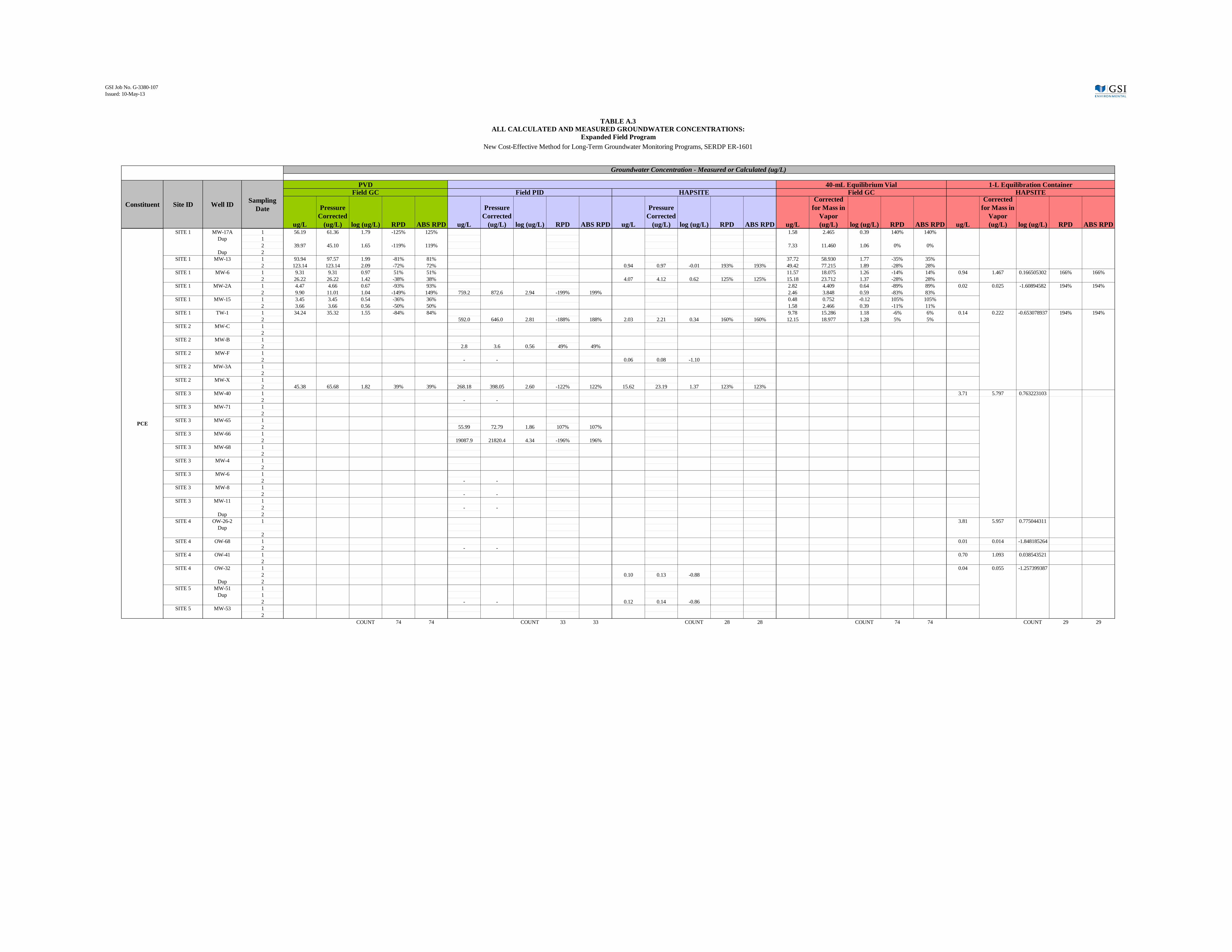
GSI Job No. G-3380-107Issued: 10-May-13
ug/L
Pressure Corrected
(ug/L) log (ug/L) RPD ABS RPD ug/L
Pressure Corrected
(ug/L) log (ug/L) RPD ABS RPD ug/L
Pressure Corrected
(ug/L) log (ug/L) RPD ABS RPD ug/L
Corrected for Mass in
Vapor (ug/L) log (ug/L) RPD ABS RPD ug/L
Corrected for Mass in
Vapor (ug/L) log (ug/L) RPD ABS RPD
PVDField GC
Constituent Site ID Well ID Sampling Date
40-mL Equilibrium Vial 1-L Equilibration ContainerField PID HAPSITE Field GC HAPSITE
TABLE A.3ALL CALCULATED AND MEASURED GROUNDWATER CONCENTRATIONS:
Expanded Field ProgramNew Cost-Effective Method for Long-Term Groundwater Monitoring Programs, SERDP ER-1601
Groundwater Concentration - Measured or Calculated (ug/L)
SITE 1 MW-17A 1 56.19 61.36 1.79 -125% 125% 1.58 2.465 0.39 140% 140%Dup 1
2 39.97 45.10 1.65 -119% 119% 7.33 11.460 1.06 0% 0%Dup 2
SITE 1 MW-13 1 93.94 97.57 1.99 -81% 81% 37.72 58.930 1.77 -35% 35%2 123.14 123.14 2.09 -72% 72% 0.94 0.97 -0.01 193% 193% 49.42 77.215 1.89 -28% 28%
SITE 1 MW-6 1 9.31 9.31 0.97 51% 51% 11.57 18.075 1.26 -14% 14% 0.94 1.467 0.166505302 166% 166%2 26.22 26.22 1.42 -38% 38% 4.07 4.12 0.62 125% 125% 15.18 23.712 1.37 -28% 28%
SITE 1 MW-2A 1 4.47 4.66 0.67 -93% 93% 2.82 4.409 0.64 -89% 89% 0.02 0.025 -1.60894582 194% 194%2 9.90 11.01 1.04 -149% 149% 759.2 872.6 2.94 -199% 199% 2.46 3.848 0.59 -83% 83%
SITE 1 MW-15 1 3.45 3.45 0.54 -36% 36% 0.48 0.752 -0.12 105% 105%2 3.66 3.66 0.56 -50% 50% 1.58 2.466 0.39 -11% 11%
SITE 1 TW-1 1 34.24 35.32 1.55 -84% 84% 9.78 15.286 1.18 -6% 6% 0.14 0.222 -0.653078937 194% 194%2 592.0 646.0 2.81 -188% 188% 2.03 2.21 0.34 160% 160% 12.15 18.977 1.28 5% 5%
SITE 2 MW-C 12
SITE 2 MW-B 12 2.8 3.6 0.56 49% 49%
SITE 2 MW-F 12 - - 0.06 0.08 -1.10
SITE 2 MW-3A 12
SITE 2 MW-X 12 45.38 65.68 1.82 39% 39% 268.18 398.05 2.60 -122% 122% 15.62 23.19 1.37 123% 123%
SITE 3 MW-40 1 3.71 5.797 0.7632231032 - -
SITE 3 MW-71 12
SITE 3 MW-65 12 55.99 72.79 1.86 107% 107%
SITE 3 MW-66 12 19087.9 21820.4 4.34 -196% 196%
SITE 3 MW-68 12
SITE 3 MW-4 12
SITE 3 MW-6 12 - -
SITE 3 MW-8 12 - -
SITE 3 MW-11 12 - -
Dup 2SITE 4 OW-26-2 1 3.81 5.957 0.775044311
Dup2
SITE 4 OW-68 1 0.01 0.014 -1.8481852642 - -
SITE 4 OW-41 1 0.70 1.093 0.0385435212
SITE 4 OW-32 1 0.04 0.055 -1.2573993872 0.10 0.13 -0.88
Dup 2SITE 5 MW-51 1
Dup 12 - - 0.12 0.14 -0.86
SITE 5 MW-53 12
COUNT 74 74 COUNT 33 33 COUNT 28 28 COUNT 74 74 COUNT 29 29
PCE

Job No.: G-3380Date Issued: 10-May-13
Sample ID Sample Date Analyte Sampling Method Analysis Method Vapor Result 1 Vapor Result 2 Vapor Result 3 unit Dilution Expected (Calculated) Groundwater Concentration (w/o Pressure Correction) unit
MW-4 4/29/2011 Vinyl Chloride Ext-Length PVD Field GC 12,732 12,491 13,000 ppmv 20 658,110 ug/LMW-4 4/29/2011 Vinyl Chloride PVD Field GC 12,843 13,525 13,169 ppmv 20 680,278 ug/LMW-4 4/29/2011 Vinyl Chloride VOA Vial Field GC 2,976 2,827 2,696 ppmv 20 141,801 ug/LMW-6 5/2/2011 Vinyl Chloride Ext-Length PVD Field GC 8,053 8,140 7,882 ppmv 1 21,794 ug/LMW-6 5/2/2011 Vinyl Chloride PVD Field GC 4,268 4,211 4,117 ppmv 1 11,372 ug/LMW-6 5/2/2011 Vinyl Chloride VOA Vial Field GC 7,331 7,497 7,483 ppmv 1 18,033 ug/LMW-8 5/2/2011 Vinyl Chloride Ext-Length PVD Field GC 5,458 6,112 5,506 ppmv 1 15,479 ug/LMW-8 5/2/2011 Vinyl Chloride PVD Field GC 5,795 5,986 5,936 ppmv 1 15,952 ug/LMW-8 5/2/2011 Vinyl Chloride VOA Vial Field GC 825 850 889 ppmv 1 2,102 ug/LMW-11 4/29/2011 Vinyl Chloride PVD Field GC 3,329 3,500 3,438 ppmv 2 17,977 ug/LMW-11 4/29/2011 Vinyl Chloride VOA Vial Field GC 5,947 5,965 6,283 ppmv 1 14,706 ug/LMW-40 4/29/2011 Vinyl Chloride Ext-Length PVD Field GC 3,780 3,559 3,669 ppmv 2 18,738 ug/LMW-40 4/29/2011 Vinyl Chloride PVD Field GC 5,965 6,142 6,100 ppmv 2 30,930 ug/LMW-40 4/29/2011 Vinyl Chloride VOA Vial Field GC 2,128 2,148 2,146 ppmv 2 9,071 ug/LMW-65 4/25/2011 Vinyl Chloride Ext-Length PVD Field GC 14,230 14,526 14,197 ppmv 10 359,932 ug/LMW-65 4/25/2011 Vinyl Chloride PVD Field GC 15,116 14,169 14,663 ppmv 10 367,902 ug/LMW-65 4/25/2011 Vinyl Chloride VOA Vial Field GC 11,125 12,066 11,340 ppmv 10 262,146 ug/LMW-66 4/29/2011 Vinyl Chloride Ext-Length PVD Field GC 8,260 8,285 8,446 ppmv 5 105,211 ug/LMW-66 4/29/2011 Vinyl Chloride PVD Field GC 6,220 6,116 6,306 ppmv 5 78,456 ug/LMW-66 4/29/2011 Vinyl Chloride VOA Vial Field GC 3,299 3,966 3,887 ppmv 5 45,545 ug/LMW-68 4/29/2011 Vinyl Chloride Ext-Length PVD Field GC 6,287 6,272 6,583 ppmv 2 33,165 ug/LMW-68 4/29/2011 Vinyl Chloride PVD Field GC 6,362 6,242 6,414 ppmv 2 32,961 ug/LMW-68 4/29/2011 Vinyl Chloride VOA Vial Field GC 1,780 2,010 2,104 ppmv 1 4,521 ug/LMW-71 4/25/2011 Vinyl Chloride Ext-Length PVD Field GC 4,145 4,232 4,283 ppmv 10 105,922 ug/LMW-71 4/25/2011 Vinyl Chloride PVD Field GC 5,858 6,031 6,360 ppmv 10 152,683 ug/LMW-71 4/25/2011 Vinyl Chloride VOA Vial Field GC 1,374 1,335 1,386 ppmv 10 30,767 ug/LMW-3A 5/2/2011 Vinyl Chloride Ext-Length PVD Field GC 712 690 709 ppmv 1 1,756 ug/LMW-3A 5/2/2011 Vinyl Chloride PVD Field GC 654 654 616 ppmv 1 1,607 ug/LMW-3A 5/2/2011 Vinyl Chloride VOA Vial Field GC 270 278 266 ppmv 1 795 ug/LMW-3A 5/2/2011 1,1-Dichloroethene Ext-Length PVD Field GC 2,894 2,901 2,924 ppmv 1 9,824 ug/LMW-3A 5/2/2011 1,1-Dichloroethene PVD Field GC 2,818 2,808 2,708 ppmv 1 9,429 ug/LMW-3A 5/2/2011 1,1-Dichloroethene VOA Vial Field GC 1,770 1,819 1,788 ppmv 1 7,447 ug/LMW-B 5/3/2011 Vinyl Chloride PVD Field GC 0.628 0.869 0.675 ppmv 1 2.01 ug/LMW-B 5/3/2011 Vinyl Chloride VOA Vial Field GC 6.280 5.826 5.801 ppmv 1 15.9 ug/LMW-B 5/3/2011 1,1-Dichloroethene Ext-Length PVD Field GC 1.988 2.004 2.050 ppmv 1 7.87 ug/LMW-B 5/3/2011 1,1-Dichloroethene PVD Field GC 16.6 17.0 16.3 ppmv 1 64.8 ug/LMW-B 5/3/2011 1,1-Dichloroethene VOA Vial Field GC 8.093 8.128 8.249 ppmv 1 30.1 ug/LMW-C 5/2/2011 Vinyl Chloride Ext-Length PVD Field GC 2.982 2.991 2.891 ppmv 1 7.67 ug/LMW-C 5/2/2011 1,1-Dichloroethene Ext-Length PVD Field GC 2.038 2.105 2.075 ppmv 1 7.40 ug/LMW-C 5/2/2011 1,1-Dichloroethene PVD Field GC 2.427 2.305 2.368 ppmv 1 8.45 ug/LMW-C 5/2/2011 1,1-Dichloroethene VOA Vial Field GC 1.691 1.408 1.360 ppmv 1 5.59 ug/LMW-F 5/2/2011 Vinyl Chloride Ext-Length PVD Field GC 3.281 3.113 3.462 ppmv 1 8.37 ug/LMW-F 5/2/2011 1,1-Dichloroethene Ext-Length PVD Field GC 0.708 0.525 1.094 ppmv 1 2.72 ug/LMW-F 5/2/2011 1,1-Dichloroethene PVD Field GC 0.719 0.598 0.639 ppmv 1 2.32 ug/LMW-F 5/2/2011 1,1-Dichloroethene VOA Vial Field GC 0.452 0.396 0.381 ppmv 1 1.27 ug/LMW-X 5/3/2011 1,1-Dichloroethene Ext-Length PVD Field GC 1.291 1.307 1.190 ppmv 1 4.45 ug/LMW-X 5/3/2011 1,1-Dichloroethene PVD Field GC 1.196 1.273 1.132 ppmv 1 4.24 ug/LMW-X 5/3/2011 1,1-Dichloroethene VOA Vial Field GC 0.475 0.497 0.547 ppmv 1 1.80 ug/LOW-26-2 4/28/2011 Vinyl Chloride Ext-Length PVD Field GC 61.7 63.9 67.9 ppmv 1 159 ug/LOW-26-2 4/28/2011 Vinyl Chloride PVD Field GC 5,174 4,996 4,689 ppmv 1 12,248 ug/LOW-26-2 4/28/2011 Vinyl Chloride VOA Vial Field GC 1,189 910 809 ppmv 1 2,604 ug/LOW-32 4/28/2011 Vinyl Chloride Ext-Length PVD Field GC 11.1 10.7 8.61 ppmv 1 25.9 ug/LOW-32 4/28/2011 Vinyl Chloride PVD Field GC 41.7 38.9 37.8 ppmv 1 101 ug/LOW-32 4/28/2011 Vinyl Chloride VOA Vial Field GC 6.31 ppmv 1 14.6 ug/LOW-41 4/28/2011 Vinyl Chloride PVD Field GC 967 807 910 ppmv 1 2,180 ug/LOW-41 4/28/2011 Vinyl Chloride VOA Vial Field GC 421 446 494 ppmv 1 988 ug/LOW-68 4/28/2011 Vinyl Chloride Ext-Length PVD Field GC 22.8 23.0 24.8 ppmv 1 56.1 ug/LOW-68 4/28/2011 Vinyl Chloride PVD Field GC 127 180 127 ppmv 1 345 ug/LOW-68 4/28/2011 Vinyl Chloride VOA Vial Field GC 18.5 20.5 20.6 ppmv 1 40.7 ug/LMW-51 4/25/2011 Trichloroethene Ext-Length PVD Field GC 0.817 0.983 ppmv 1 12.6 ug/LMW-51 4/25/2011 Trichloroethene PVD Field GC 1.189 0.968 0.928 ppmv 1 14.4 ug/LMW-51 4/25/2011 Trichloroethene VOA Vial Field GC 1.705 1.640 1.674 ppmv 1 16.2 ug/LMW-53 5/3/2011 Trichloroethene Ext-Length PVD Field GC 200 200 197 ppmv 1 3,243 ug/LMW-53 5/3/2011 Trichloroethene PVD Field GC 374 356 358 ppmv 1 5,925 ug/LMW-53 5/3/2011 Trichloroethene VOA Vial Field GC 300 293 288 ppmv 1 4,819 ug/LMW-2A 4/27/2011 Vinyl Chloride Ext-Length PVD Field GC 3.791 3.872 ppmv 1 8.74 ug/LMW-2A 4/27/2011 1,1-Dichloroethene Ext-Length PVD Field GC 0.976 0.914 ppmv 1 2.88 ug/LMW-2A 4/27/2011 1,1-Dichloroethene PVD Field GC 0.827 0.839 ppmv 1 2.53 ug/LMW-2A 4/27/2011 1,1-Dichloroethene VOA Vial Field GC 0.207 0.212 ppmv 1 0.593 ug/LMW-2A 4/27/2011 Benzene Ext-Length PVD Field GC 3.836 3.812 ppmv 1 47.0 ug/LMW-2A 4/27/2011 Benzene PVD Field GC 2.878 2.692 ppmv 1 34.2 ug/LMW-2A 4/27/2011 Benzene VOA Vial Field GC 1.886 2.063 ppmv 1 22.4 ug/LMW-2A 4/27/2011 Tetrachloroethene Ext-Length PVD Field GC 0.857 0.560 ppmv 1 6.34 ug/LMW-2A 4/27/2011 Tetrachloroethene PVD Field GC 0.546 0.453 ppmv 1 4.47 ug/LMW-2A 4/27/2011 Tetrachloroethene VOA Vial Field GC 0.320 0.372 ppmv 1 2.82 ug/LMW-6 4/27/2011 1,1-Dichloroethene Ext-Length PVD Field GC 0.379 0.394 ppmv 1 1.25 ug/LMW-6 4/27/2011 1,1-Dichloroethene PVD Field GC 0.565 0.600 ppmv 1 1.88 ug/LMW-6 4/27/2011 1,1-Dichloroethene VOA Vial Field GC 0.629 0.670 ppmv 1 1.71 ug/LMW-6 4/27/2011 Benzene Ext-Length PVD Field GC 1.581 1.604 ppmv 1 20.8 ug/LMW-6 4/27/2011 Benzene PVD Field GC 1.346 1.361 ppmv 1 17.7 ug/LMW-6 4/27/2011 Benzene VOA Vial Field GC 5.984 5.748 ppmv 1 62 ug/LMW-6 4/27/2011 Trichloroethene Ext-Length PVD Field GC 0.622 0.646 ppmv 1 8.28 ug/LMW-6 4/27/2011 Trichloroethene PVD Field GC 0.346 0.380 ppmv 1 4.73 ug/LMW-6 4/27/2011 Trichloroethene VOA Vial Field GC 0.755 0.746 ppmv 1 7.73 ug/LMW-6 4/27/2011 Tetrachloroethene Ext-Length PVD Field GC 1.372 1.445 ppmv 1 13.5 ug/LMW-6 4/27/2011 Tetrachloroethene PVD Field GC 1.000 0.943 ppmv 1 9.31 ug/LMW-6 4/27/2011 Tetrachloroethene VOA Vial Field GC 1.616 1.470 ppmv 1 11.6 ug/LMW-13 4/26/2011 1,1-Dichloroethene Ext-Length PVD Field GC 1.984 ppmv 1 6.67 ug/LMW-13 4/26/2011 1,1-Dichloroethene PVD Field GC 8.690 8.644 ppmv 1 29.1 ug/LMW-13 4/26/2011 1,1-Dichloroethene VOA Vial Field GC 2.676 2.638 ppmv 1 7.85 ug/LMW-13 4/26/2011 Benzene Ext-Length PVD Field GC 1.898 ppmv 1 25.9 ug/LMW-13 4/26/2011 Benzene PVD Field GC 7.769 7.422 ppmv 1 104 ug/LMW-13 4/26/2011 Benzene VOA Vial Field GC 4.542 4.755 ppmv 1 55.3 ug/LMW-13 4/26/2011 Trichloroethene Ext-Length PVD Field GC 0.769 ppmv 1 10.5 ug/LMW-13 4/26/2011 Trichloroethene PVD Field GC 5.079 5.128 ppmv 1 69.8 ug/LMW-13 4/26/2011 Trichloroethene VOA Vial Field GC 2.192 2.426 ppmv 1 27.1 ug/LMW-13 4/26/2011 Tetrachloroethene Ext-Length PVD Field GC 0.870 ppmv 1 8.78 ug/LMW-13 4/26/2011 Tetrachloroethene PVD Field GC 9.946 8.697 ppmv 1 93.9 ug/LMW-13 4/26/2011 Tetrachloroethene VOA Vial Field GC 4.579 4.193 ppmv 1 37.7 ug/LMW-15 4/26/2011 Benzene Ext-Length PVD Field GC 0.104 0.173 ppmv 1 1.87 ug/LMW-15 4/26/2011 Benzene PVD Field GC 0.128 0.234 ppmv 1 2.44 ug/LMW-15 4/26/2011 Benzene VOA Vial Field GC 0.109 0.119 ppmv 1 1.30 ug/LMW-15 4/26/2011 Tetrachloroethene Ext-Length PVD Field GC 0.350 0.342 ppmv 1 3.44 ug/LMW-15 4/26/2011 Tetrachloroethene PVD Field GC 0.358 0.338 ppmv 1 3.45 ug/LMW-15 4/26/2011 Tetrachloroethene VOA Vial Field GC 0.063 0.055 ppmv 1 0.481 ug/LMW-17A 4/26/2011 1,1-Dichloroethene PVD Field GC 1.378 1.351 1.377 ppmv 1 4.53 ug/LMW-17A 4/26/2011 Benzene PVD Field GC 1.405 1.756 1.478 ppmv 1 20.8 ug/LMW-17A 4/26/2011 Benzene VOA Vial Field GC 0.108 0.220 0.109 ppmv 1 1.40 ug/LMW-17A 4/26/2011 Tetrachloroethene Ext-Length PVD Field GC 2.405 2.501 2.439 ppmv 1 24.3 ug/LMW-17A 4/26/2011 Tetrachloroethene PVD Field GC 5.064 5.899 6.001 ppmv 1 56.2 ug/LMW-17A 4/26/2011 Tetrachloroethene VOA Vial Field GC 0.117 0.257 0.330 ppmv 1 1.58 ug/LTW-1 4/27/2011 1,1-Dichloroethene Ext-Length PVD Field GC 0.962 0.860 ppmv 1 2.97 ug/LTW-1 4/27/2011 1,1-Dichloroethene PVD Field GC 1.068 0.908 ppmv 1 3.22 ug/LTW-1 4/27/2011 1,1-Dichloroethene VOA Vial Field GC 0.375 0.334 ppmv 1 0.960 ug/LTW-1 4/27/2011 Benzene Ext-Length PVD Field GC 1.273 0.827 ppmv 1 13.9 ug/L
TABLE A.4ALL VAPOR ANALYSES:Expanded Field Program
New Cost-Effective Method for Long-Term Groundwater Monitoring Programs, SERDP ER-1601

Job No.: G-3380Date Issued: 10-May-13
Sample ID Sample Date Analyte Sampling Method Analysis Method Vapor Result 1 Vapor Result 2 Vapor Result 3 unit Dilution Expected (Calculated) Groundwater Concentration (w/o Pressure Correction) unit
TABLE A.4ALL VAPOR ANALYSES:Expanded Field Program
New Cost-Effective Method for Long-Term Groundwater Monitoring Programs, SERDP ER-1601
TW-1 4/27/2011 Benzene PVD Field GC 0.782 0.722 ppmv 1 9.9 ug/LTW-1 4/27/2011 Benzene VOA Vial Field GC 0.764 0.634 ppmv 1 7.6 ug/LTW-1 4/27/2011 Trichloroethene Ext-Length PVD Field GC 2.436 1.307 ppmv 1 24.7 ug/LTW-1 4/27/2011 Trichloroethene PVD Field GC 1.152 1.129 ppmv 1 15.0 ug/LTW-1 4/27/2011 Trichloroethene VOA Vial Field GC 0.673 0.578 ppmv 1 6.64 ug/LTW-1 4/27/2011 Tetrachloroethene Ext-Length PVD Field GC 4.420 2.714 ppmv 1 34.6 ug/LTW-1 4/27/2011 Tetrachloroethene PVD Field GC 3.564 3.497 ppmv 1 34.2 ug/LTW-1 4/27/2011 Tetrachloroethene VOA Vial Field GC 1.482 1.047 ppmv 1 9.78 ug/LMW-4 5/16/2011 Vinyl Chloride PVD Field GC 11,044 9,908 10,501 ppmv 20 536,537 ug/LMW-4 5/16/2011 Vinyl Chloride VOA Vial Field GC 7,922 7,743 8,142 ppmv 20 313,147 ug/LMW-6 5/16/2011 Vinyl Chloride Hass Sampler Field GC 25,388 25,060 23,191 ppmv 1 65,007 ug/LMW-6 5/19/2011 Vinyl Chloride PVD Field GC 11,289 10,118 11,012 ppmv 1 28,667 ug/LMW-6 5/19/2011 Vinyl Chloride VOA Vial Field GC 10,986 9,722 10,987 ppmv 1 23,166 ug/LMW-8 5/19/2011 Vinyl Chloride Hass Sampler Field GC 2,956 2,485 2,372 ppmv 1 6,836 ug/LMW-8 5/19/2011 Vinyl Chloride PVD Field GC 8,724 6,919 8,726 ppmv 1 21,356 ug/LMW-8 5/19/2011 Vinyl Chloride VOA Vial Field GC 1,142 1,238 1,195 ppmv 1 2,677 ug/LMW-11 5/16/2011 Vinyl Chloride Hass Sampler Field GC 12,749 12,709 12,638 ppmv 2 67,959 ug/LMW-11 5/16/2011 Vinyl Chloride PVD Field GC 10,494 10,624 10,380 ppmv 2 56,189 ug/LMW-11 5/16/2011 Vinyl Chloride VOA Vial Field GC 6,711 6,935 7,526 ppmv 1 16,816 ug/LMW-40 5/16/2011 Vinyl Chloride Hass Sampler Field GC 5,423 5,099 4,943 ppmv 2 27,431 ug/LMW-40 5/16/2011 Vinyl Chloride PVD Field GC 6,547 6,715 6,492 ppmv 2 35,027 ug/LMW-40 5/16/2011 Vinyl Chloride VOA Vial Field GC 4,832 4,897 4,888 ppmv 1 10,683 ug/LMW-65 5/19/2011 Vinyl Chloride Hass Sampler Field GC 13,904 11,708 12,062 ppmv 10 335,395 ug/LMW-65 5/19/2011 Vinyl Chloride PVD Field GC 17,466 15,264 21,468 ppmv 10 481,855 ug/LMW-65 5/19/2011 Vinyl Chloride VOA Vial Field GC 9,357 11,402 8,763 ppmv 10 224,897 ug/LMW-66 5/16/2011 Vinyl Chloride Hass Sampler Field GC 7,227 7,164 6,942 ppmv 5 91,497 ug/LMW-66 5/16/2011 Vinyl Chloride PVD Field GC 11,450 10,953 10,627 ppmv 5 141,245 ug/LMW-66 5/16/2011 Vinyl Chloride VOA Vial Field GC 4,051 4,326 4,091 ppmv 5 44,635 ug/LMW-68 5/16/2011 Vinyl Chloride Hass Sampler Field GC 10,932 10,648 10,972 ppmv 1 28,014 ug/LMW-68 5/16/2011 Vinyl Chloride PVD Field GC 11,903 11,598 11,595 ppmv 1 30,164 ug/LMW-68 5/16/2011 Vinyl Chloride VOA Vial Field GC 4,607 4,644 4,919 ppmv 1 9,542 ug/LMW-71 5/19/2011 Vinyl Chloride Hass Sampler Field GC 401 485 520 ppmv 10 12,043 ug/LMW-71 5/19/2011 Vinyl Chloride PVD Field GC 2,327 2,275 2,007 ppmv 10 56,739 ug/LMW-71 5/19/2011 Vinyl Chloride VOA Vial Field GC 877 778 659 ppmv 10 17,088 ug/LMW-3A 5/20/2011 Vinyl Chloride Hass Sampler Field GC 43.4 50.7 48.7 ppmv 1 112 ug/LMW-3A 5/20/2011 Vinyl Chloride PVD Field GC 753 757 801 ppmv 1 1,819 ug/LMW-3A 5/20/2011 Vinyl Chloride VOA Vial Field GC 390 357 381 ppmv 1 760 ug/LMW-3A 5/20/2011 1,1-Dichloroethene Hass Sampler Field GC 634 689 672 ppmv 1 2,150 ug/LMW-3A 5/20/2011 1,1-Dichloroethene PVD Field GC 3,483 3,554 3,632 ppmv 1 11,508 ug/LMW-3A 5/20/2011 1,1-Dichloroethene VOA Vial Field GC 2,008 2,009 1,967 ppmv 1 5,280 ug/LMW-B 5/20/2011 Vinyl Chloride Hass Sampler Field GC 0.565 0.486 0.455 ppmv 1 1.30 ug/LMW-B 5/20/2011 Vinyl Chloride PVD Field GC 1.03 1.06 1.15 ppmv 1 2.77 ug/LMW-B 5/20/2011 Vinyl Chloride VOA Vial Field GC 2.66 2.57 2.93 ppmv 1 5.46 ug/LMW-B 5/20/2011 1,1-Dichloroethene Hass Sampler Field GC 19.2 16.6 15.8 ppmv 1 61.4 ug/LMW-B 5/20/2011 1,1-Dichloroethene PVD Field GC 13.8 13.6 14.5 ppmv 1 49.6 ug/LMW-B 5/20/2011 1,1-Dichloroethene VOA Vial Field GC 13.1 13.0 15.3 ppmv 1 35.5 ug/LMW-C 5/20/2011 1,1-Dichloroethene Hass Sampler Field GC 0.741 0.622 0.694 ppmv 1 2.14 ug/LMW-C 5/20/2011 1,1-Dichloroethene PVD Field GC 1.78 1.55 2.05 ppmv 1 5.60 ug/LMW-C 5/20/2011 1,1-Dichloroethene VOA Vial Field GC 2.17 1.87 1.88 ppmv 1 5.06 ug/LMW-F 5/20/2011 1,1-Dichloroethene Hass Sampler Field GC 0.429 0.410 0.415 ppmv 1 1.54 ug/LMW-F 5/20/2011 1,1-Dichloroethene PVD Field GC 0.375 0.381 0.383 ppmv 1 1.39 ug/LMW-F 5/20/2011 1,1-Dichloroethene VOA Vial Field GC 0.399 0.350 0.383 ppmv 1 0.98 ug/LMW-X 5/20/2011 1,1-Dichloroethene Hass Sampler Field GC 1.24 1.25 1.25 ppmv 1 4.46 ug/LMW-X 5/20/2011 1,1-Dichloroethene PVD Field GC 1.47 1.37 1.39 ppmv 1 5.03 ug/LMW-X 5/20/2011 1,1-Dichloroethene VOA Vial Field GC 1.69 1.76 1.82 ppmv 1 4.80 ug/LOW-26-2 5/17/2011 Vinyl Chloride PVD Field GC 4,668 4,483 3,838 ppmv 1 10,643 ug/LOW-26-2 5/17/2011 Vinyl Chloride VOA Vial Field GC 8,389 8,789 6,880 ppmv 1 18,909 ug/LOW-32 5/17/2011 Vinyl Chloride Hass Sampler Field GC 18.0 22.7 25.4 ppmv 1 57.0 ug/LOW-32 5/17/2011 Vinyl Chloride PVD Field GC 57.6 65.0 60.0 ppmv 1 157 ug/LOW-32 5/17/2011 Vinyl Chloride VOA Vial Field GC 85.5 84.2 99.0 ppmv 1 195 ug/LOW-41 5/17/2011 Vinyl Chloride PVD Field GC 2,486 2,108 2,127 ppmv 1 5,751 ug/LOW-41 5/17/2011 Vinyl Chloride VOA Vial Field GC 745 645 806 ppmv 1 1,673 ug/LOW-68 5/17/2011 Vinyl Chloride Hass Sampler Field GC 101 103 105 ppmv 1 252 ug/LOW-68 5/17/2011 Vinyl Chloride PVD Field GC 206 194 215 ppmv 1 502 ug/LOW-68 5/17/2011 Vinyl Chloride VOA Vial Field GC 18.3 18.6 18.7 ppmv 1 40.9 ug/LMW-51 5/19/2011 Trichloroethene Hass Sampler Field GC 3.93 3.34 2.94 ppmv 1 52.2 ug/LMW-51 5/19/2011 Trichloroethene PVD Field GC 3.51 3.51 3.33 ppmv 1 52.9 ug/LMW-51 5/19/2011 Trichloroethene VOA Vial Field GC 2.74 2.76 2.93 ppmv 1 36.6 ug/LMW-53 5/19/2011 Trichloroethene Hass Sampler Field GC 271 283 299 ppmv 1 4,135 ug/LMW-53 5/19/2011 Trichloroethene PVD Field GC 1,234 1,299 1,165 ppmv 1 17,915 ug/LMW-53 5/19/2011 Trichloroethene VOA Vial Field GC 776 879 877 ppmv 1 10,075 ug/LMW-2A 5/18/2011 1,1-Dichloroethene Hass Sampler Field GC 1.37 1.28 ppmv 1 4.27 ug/LMW-2A 5/18/2011 1,1-Dichloroethene PVD Field GC 1.32 1.36 ppmv 1 4.33 ug/LMW-2A 5/18/2011 1,1-Dichloroethene VOA Vial Field GC 0.207 0.214 ppmv 1 0.525 ug/LMW-2A 5/18/2011 Benzene Hass Sampler Field GC 3.94 3.68 ppmv 1 49.9 ug/LMW-2A 5/18/2011 Benzene PVD Field GC 4.14 4.44 ppmv 1 56.2 ug/LMW-2A 5/18/2011 Benzene VOA Vial Field GC 1.92 1.84 ppmv 1 18.7 ug/LMW-2A 5/18/2011 Trichloroethene Hass Sampler Field GC 0.481 0.409 ppmv 1 5.82 ug/LMW-2A 5/18/2011 Trichloroethene PVD Field GC 0.489 0.471 ppmv 1 6.29 ug/LMW-2A 5/18/2011 Trichloroethene VOA Vial Field GC 0.135 0.186 ppmv 1 1.55 ug/LMW-2A 5/18/2011 Tetrachloroethene Hass Sampler Field GC 0.983 0.608 ppmv 1 7.65 ug/LMW-2A 5/18/2011 Tetrachloroethene PVD Field GC 0.940 1.12 ppmv 1 9.90 ug/LMW-2A 5/18/2011 Tetrachloroethene VOA Vial Field GC 0.393 0.310 ppmv 1 2.46 ug/LMW-6 5/18/2011 1,1-Dichloroethene Hass Sampler Field GC 0.965 1.40 ppmv 1 4.16 ug/LMW-6 5/18/2011 1,1-Dichloroethene PVD Field GC 1.12 1.13 ppmv 1 3.95 ug/LMW-6 5/18/2011 1,1-Dichloroethene VOA Vial Field GC 0.761 0.764 ppmv 1 2.07 ug/LMW-6 5/18/2011 Benzene Hass Sampler Field GC 2.78 4.22 ppmv 1 50.3 ug/LMW-6 5/18/2011 Benzene PVD Field GC 4.31 4.42 ppmv 1 62.4 ug/LMW-6 5/18/2011 Benzene VOA Vial Field GC 6.50 6.62 ppmv 1 71.1 ug/LMW-6 5/18/2011 Trichloroethene Hass Sampler Field GC 0.936 1.34 ppmv 1 16.4 ug/LMW-6 5/18/2011 Trichloroethene PVD Field GC 0.874 0.914 ppmv 1 12.9 ug/LMW-6 5/18/2011 Trichloroethene VOA Vial Field GC 0.990 1.03 ppmv 1 10.7 ug/LMW-6 5/18/2011 Tetrachloroethene Hass Sampler Field GC 1.24 1.58 ppmv 1 15.0 ug/LMW-6 5/18/2011 Tetrachloroethene PVD Field GC 2.24 2.69 ppmv 1 26.2 ug/LMW-6 5/18/2011 Tetrachloroethene VOA Vial Field GC 2.00 1.92 ppmv 1 15.2 ug/LMW-13 5/18/2011 1,1-Dichloroethene Hass Sampler Field GC 3.16 2.69 ppmv 1 10.1 ug/LMW-13 5/18/2011 1,1-Dichloroethene PVD Field GC 6.37 8.57 ppmv 1 25.9 ug/LMW-13 5/18/2011 1,1-Dichloroethene VOA Vial Field GC 3.38 3.56 ppmv 1 9.64 ug/LMW-13 5/18/2011 Benzene Hass Sampler Field GC 3.19 2.88 ppmv 1 42.7 ug/LMW-13 5/18/2011 Benzene PVD Field GC 4.79 6.15 ppmv 1 77.2 ug/LMW-13 5/18/2011 Benzene VOA Vial Field GC 4.99 5.17 ppmv 1 56.7 ug/LMW-13 5/18/2011 Trichloroethene Hass Sampler Field GC 1.22 1.10 ppmv 1 16.4 ug/LMW-13 5/18/2011 Trichloroethene PVD Field GC 3.69 4.70 ppmv 1 59.6 ug/LMW-13 5/18/2011 Trichloroethene VOA Vial Field GC 3.04 3.01 ppmv 1 33.1 ug/LMW-13 5/18/2011 Tetrachloroethene Hass Sampler Field GC 0.481 0.469 ppmv 1 4.96 ug/LMW-13 5/18/2011 Tetrachloroethene PVD Field GC 10.4 13.1 ppmv 1 123 ug/LMW-13 5/18/2011 Tetrachloroethene VOA Vial Field GC 6.68 5.70 ppmv 1 49.4 ug/LMW-15 5/18/2011 Benzene PVD Field GC 0.228 0.236 ppmv 1 3.41 ug/LMW-15 5/18/2011 Benzene VOA Vial Field GC 0.212 0.244 ppmv 1 2.70 ug/LMW-15 5/18/2011 Trichloroethene PVD Field GC 0.174 0.219 ppmv 1 2.92 ug/LMW-15 5/18/2011 Trichloroethene VOA Vial Field GC 0.168 0.193 ppmv 1 2.11 ug/LMW-15 5/18/2011 Tetrachloroethene Hass Sampler Field GC 0.139 0.096 ppmv 1 1.30 ug/LMW-15 5/18/2011 Tetrachloroethene PVD Field GC 0.318 0.349 ppmv 1 3.66 ug/LMW-15 5/18/2011 Tetrachloroethene VOA Vial Field GC 0.190 0.179 ppmv 1 1.58 ug/LMW-17A 5/18/2011 1,1-Dichloroethene Hass Sampler Field GC 0.705 ppmv 1 2.55 ug/L
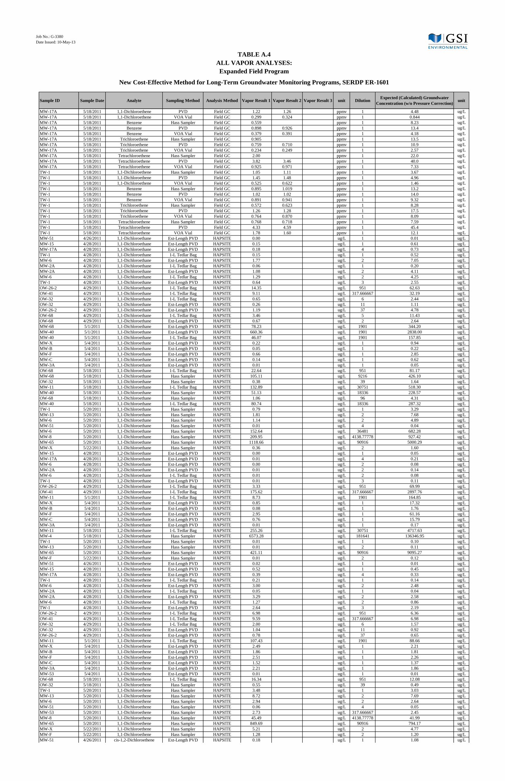
Job No.: G-3380Date Issued: 10-May-13
Sample ID Sample Date Analyte Sampling Method Analysis Method Vapor Result 1 Vapor Result 2 Vapor Result 3 unit Dilution Expected (Calculated) Groundwater Concentration (w/o Pressure Correction) unit
TABLE A.4ALL VAPOR ANALYSES:Expanded Field Program
New Cost-Effective Method for Long-Term Groundwater Monitoring Programs, SERDP ER-1601
MW-17A 5/18/2011 1,1-Dichloroethene PVD Field GC 1.22 1.26 ppmv 1 4.48 ug/LMW-17A 5/18/2011 1,1-Dichloroethene VOA Vial Field GC 0.299 0.324 ppmv 1 0.844 ug/LMW-17A 5/18/2011 Benzene Hass Sampler Field GC 0.559 ppmv 1 8.23 ug/LMW-17A 5/18/2011 Benzene PVD Field GC 0.898 0.926 ppmv 1 13.4 ug/LMW-17A 5/18/2011 Benzene VOA Vial Field GC 0.379 0.391 ppmv 1 4.18 ug/LMW-17A 5/18/2011 Trichloroethene Hass Sampler Field GC 0.905 ppmv 1 13.5 ug/LMW-17A 5/18/2011 Trichloroethene PVD Field GC 0.759 0.710 ppmv 1 10.9 ug/LMW-17A 5/18/2011 Trichloroethene VOA Vial Field GC 0.234 0.249 ppmv 1 2.57 ug/LMW-17A 5/18/2011 Tetrachloroethene Hass Sampler Field GC 2.00 ppmv 1 22.0 ug/LMW-17A 5/18/2011 Tetrachloroethene PVD Field GC 3.82 3.46 ppmv 1 40.0 ug/LMW-17A 5/18/2011 Tetrachloroethene VOA Vial Field GC 0.925 0.971 ppmv 1 7.33 ug/LTW-1 5/18/2011 1,1-Dichloroethene Hass Sampler Field GC 1.05 1.11 ppmv 1 3.67 ug/LTW-1 5/18/2011 1,1-Dichloroethene PVD Field GC 1.45 1.48 ppmv 1 4.96 ug/LTW-1 5/18/2011 1,1-Dichloroethene VOA Vial Field GC 0.525 0.622 ppmv 1 1.46 ug/LTW-1 5/18/2011 Benzene Hass Sampler Field GC 0.895 1.019 ppmv 1 13.2 ug/LTW-1 5/18/2011 Benzene PVD Field GC 1.02 1.02 ppmv 1 14.0 ug/LTW-1 5/18/2011 Benzene VOA Vial Field GC 0.891 0.941 ppmv 1 9.32 ug/LTW-1 5/18/2011 Trichloroethene Hass Sampler Field GC 0.572 0.623 ppmv 1 8.28 ug/LTW-1 5/18/2011 Trichloroethene PVD Field GC 1.26 1.28 ppmv 1 17.5 ug/LTW-1 5/18/2011 Trichloroethene VOA Vial Field GC 0.764 0.870 ppmv 1 8.09 ug/LTW-1 5/18/2011 Tetrachloroethene Hass Sampler Field GC 0.768 0.718 ppmv 1 7.59 ug/LTW-1 5/18/2011 Tetrachloroethene PVD Field GC 4.33 4.59 ppmv 1 45.4 ug/LTW-1 5/18/2011 Tetrachloroethene VOA Vial Field GC 1.78 1.60 ppmv 1 12.1 ug/LMW-51 4/26/2011 1,1-Dichloroethane Ext-Length PVD HAPSITE 0.00 ug/L 1 0.01 ug/LMW-15 4/28/2011 1,1-Dichloroethane Ext-Length PVD HAPSITE 0.15 ug/L 1 0.61 ug/LMW-17A 4/28/2011 1,1-Dichloroethane Ext-Length PVD HAPSITE 0.18 ug/L 4 0.73 ug/LTW-1 4/28/2011 1,1-Dichloroethane 1-L Tedlar Bag HAPSITE 0.15 ug/L 1 0.52 ug/LMW-6 4/28/2011 1,1-Dichloroethane Ext-Length PVD HAPSITE 1.77 ug/L 2 7.05 ug/LMW-2A 4/28/2011 1,1-Dichloroethane 1-L Tedlar Bag HAPSITE 0.06 ug/L 1 0.20 ug/LMW-2A 4/28/2011 1,1-Dichloroethane Ext-Length PVD HAPSITE 1.08 ug/L 2 4.11 ug/LMW-6 4/28/2011 1,1-Dichloroethane 1-L Tedlar Bag HAPSITE 1.29 ug/L 2 4.25 ug/LTW-1 4/28/2011 1,1-Dichloroethane Ext-Length PVD HAPSITE 0.64 ug/L 3 2.55 ug/LOW-26-2 4/29/2011 1,1-Dichloroethane 1-L Tedlar Bag HAPSITE 14.35 ug/L 951 62.63 ug/LOW-41 4/29/2011 1,1-Dichloroethane 1-L Tedlar Bag HAPSITE 9.11 ug/L 317.666667 32.19 ug/LOW-32 4/29/2011 1,1-Dichloroethane 1-L Tedlar Bag HAPSITE 0.65 ug/L 6 2.44 ug/LOW-32 4/29/2011 1,1-Dichloroethane Ext-Length PVD HAPSITE 0.26 ug/L 11 1.11 ug/LOW-26-2 4/29/2011 1,1-Dichloroethane Ext-Length PVD HAPSITE 1.19 ug/L 37 4.78 ug/LOW-68 4/29/2011 1,1-Dichloroethane 1-L Tedlar Bag HAPSITE 3.46 ug/L 5 11.43 ug/LOW-68 4/29/2011 1,1-Dichloroethane Ext-Length PVD HAPSITE 0.67 ug/L 2 2.64 ug/LMW-68 5/1/2011 1,1-Dichloroethane Ext-Length PVD HAPSITE 78.23 ug/L 1901 344.20 ug/LMW-40 5/1/2011 1,1-Dichloroethane Ext-Length PVD HAPSITE 660.36 ug/L 1901 2838.00 ug/LMW-40 5/1/2011 1,1-Dichloroethane 1-L Tedlar Bag HAPSITE 46.07 ug/L 1901 157.85 ug/LMW-X 5/4/2011 1,1-Dichloroethane Ext-Length PVD HAPSITE 0.22 ug/L 1 0.94 ug/LMW-B 5/4/2011 1,1-Dichloroethane Ext-Length PVD HAPSITE 0.05 ug/L 1 0.22 ug/LMW-F 5/4/2011 1,1-Dichloroethane Ext-Length PVD HAPSITE 0.66 ug/L 1 2.85 ug/LMW-C 5/4/2011 1,1-Dichloroethane Ext-Length PVD HAPSITE 0.14 ug/L 1 0.62 ug/LMW-3A 5/4/2011 1,1-Dichloroethane Ext-Length PVD HAPSITE 0.01 ug/L 1 0.05 ug/LOW-68 5/18/2011 1,1-Dichloroethane 1-L Tedlar Bag HAPSITE 22.64 ug/L 951 81.17 ug/LMW-68 5/18/2011 1,1-Dichloroethane Hass Sampler HAPSITE 105.11 ug/L 9216 426.10 ug/LOW-32 5/18/2011 1,1-Dichloroethane Hass Sampler HAPSITE 0.38 ug/L 39 1.64 ug/LMW-11 5/18/2011 1,1-Dichloroethane 1-L Tedlar Bag HAPSITE 132.89 ug/L 30751 518.30 ug/LMW-40 5/18/2011 1,1-Dichloroethane Hass Sampler HAPSITE 51.13 ug/L 18336 228.57 ug/LOW-68 5/18/2011 1,1-Dichloroethane Hass Sampler HAPSITE 1.06 ug/L 96 4.31 ug/LMW-40 5/18/2011 1,1-Dichloroethane 1-L Tedlar Bag HAPSITE 80.74 ug/L 18336 287.32 ug/LTW-1 5/20/2011 1,1-Dichloroethane Hass Sampler HAPSITE 0.79 ug/L 1 3.29 ug/LMW-13 5/20/2011 1,1-Dichloroethane Hass Sampler HAPSITE 1.81 ug/L 2 7.68 ug/LMW-6 5/20/2011 1,1-Dichloroethane Hass Sampler HAPSITE 1.14 ug/L 2 4.89 ug/LMW-51 5/20/2011 1,1-Dichloroethane Hass Sampler HAPSITE 0.01 ug/L 4 0.04 ug/LMW-6 5/20/2011 1,1-Dichloroethane Hass Sampler HAPSITE 152.64 ug/L 36481 682.28 ug/LMW-8 5/20/2011 1,1-Dichloroethane Hass Sampler HAPSITE 209.95 ug/L 4138.77778 927.42 ug/LMW-65 5/20/2011 1,1-Dichloroethane Hass Sampler HAPSITE 1118.66 ug/L 90916 5000.29 ug/LMW-X 5/22/2011 1,1-Dichloroethane Hass Sampler HAPSITE 0.36 ug/L 2 1.60 ug/LMW-15 4/28/2011 1,2-Dichloroethane Ext-Length PVD HAPSITE 0.00 ug/L 1 0.05 ug/LMW-17A 4/28/2011 1,2-Dichloroethane Ext-Length PVD HAPSITE 0.01 ug/L 4 0.21 ug/LMW-6 4/28/2011 1,2-Dichloroethane Ext-Length PVD HAPSITE 0.00 ug/L 2 0.08 ug/LMW-2A 4/28/2011 1,2-Dichloroethane Ext-Length PVD HAPSITE 0.01 ug/L 2 0.14 ug/LMW-6 4/28/2011 1,2-Dichloroethane 1-L Tedlar Bag HAPSITE 0.01 ug/L 2 0.08 ug/LTW-1 4/28/2011 1,2-Dichloroethane Ext-Length PVD HAPSITE 0.01 ug/L 3 0.11 ug/LOW-26-2 4/29/2011 1,2-Dichloroethane 1-L Tedlar Bag HAPSITE 3.33 ug/L 951 69.99 ug/LOW-41 4/29/2011 1,2-Dichloroethane 1-L Tedlar Bag HAPSITE 175.62 ug/L 317.666667 2897.76 ug/LMW-11 5/1/2011 1,2-Dichloroethane 1-L Tedlar Bag HAPSITE 8.73 ug/L 1901 164.85 ug/LMW-X 5/4/2011 1,2-Dichloroethane Ext-Length PVD HAPSITE 0.85 ug/L 1 17.32 ug/LMW-B 5/4/2011 1,2-Dichloroethane Ext-Length PVD HAPSITE 0.08 ug/L 1 1.76 ug/LMW-F 5/4/2011 1,2-Dichloroethane Ext-Length PVD HAPSITE 2.95 ug/L 1 61.16 ug/LMW-C 5/4/2011 1,2-Dichloroethane Ext-Length PVD HAPSITE 0.76 ug/L 1 15.79 ug/LMW-3A 5/4/2011 1,2-Dichloroethane Ext-Length PVD HAPSITE 0.01 ug/L 1 0.17 ug/LMW-11 5/18/2011 1,2-Dichloroethane 1-L Tedlar Bag HAPSITE 255.26 ug/L 30751 4717.63 ug/LMW-4 5/18/2011 1,2-Dichloroethane Hass Sampler HAPSITE 6573.28 ug/L 181641 136346.95 ug/LTW-1 5/20/2011 1,2-Dichloroethane Hass Sampler HAPSITE 0.01 ug/L 1 0.10 ug/LMW-13 5/20/2011 1,2-Dichloroethane Hass Sampler HAPSITE 0.01 ug/L 2 0.11 ug/LMW-65 5/20/2011 1,2-Dichloroethane Hass Sampler HAPSITE 421.11 ug/L 90916 9095.27 ug/LMW-F 5/22/2011 1,2-Dichloroethane Hass Sampler HAPSITE 0.01 ug/L 2 0.12 ug/LMW-51 4/26/2011 1,1-Dichloroethene Ext-Length PVD HAPSITE 0.02 ug/L 1 0.01 ug/LMW-15 4/28/2011 1,1-Dichloroethene Ext-Length PVD HAPSITE 0.52 ug/L 1 0.45 ug/LMW-17A 4/28/2011 1,1-Dichloroethene Ext-Length PVD HAPSITE 0.39 ug/L 4 0.33 ug/LTW-1 4/28/2011 1,1-Dichloroethene 1-L Tedlar Bag HAPSITE 0.21 ug/L 1 0.14 ug/LMW-6 4/28/2011 1,1-Dichloroethene Ext-Length PVD HAPSITE 3.00 ug/L 2 2.48 ug/LMW-2A 4/28/2011 1,1-Dichloroethene 1-L Tedlar Bag HAPSITE 0.05 ug/L 1 0.04 ug/LMW-2A 4/28/2011 1,1-Dichloroethene Ext-Length PVD HAPSITE 3.29 ug/L 2 2.58 ug/LMW-6 4/28/2011 1,1-Dichloroethene 1-L Tedlar Bag HAPSITE 1.27 ug/L 2 0.86 ug/LTW-1 4/28/2011 1,1-Dichloroethene Ext-Length PVD HAPSITE 2.64 ug/L 3 2.19 ug/LOW-26-2 4/29/2011 1,1-Dichloroethene 1-L Tedlar Bag HAPSITE 6.98 ug/L 951 6.36 ug/LOW-41 4/29/2011 1,1-Dichloroethene 1-L Tedlar Bag HAPSITE 9.59 ug/L 317.666667 6.98 ug/LOW-32 4/29/2011 1,1-Dichloroethene 1-L Tedlar Bag HAPSITE 2.00 ug/L 6 1.57 ug/LOW-32 4/29/2011 1,1-Dichloroethene Ext-Length PVD HAPSITE 1.04 ug/L 11 0.92 ug/LOW-26-2 4/29/2011 1,1-Dichloroethene Ext-Length PVD HAPSITE 0.78 ug/L 37 0.65 ug/LMW-11 5/1/2011 1,1-Dichloroethene 1-L Tedlar Bag HAPSITE 107.43 ug/L 1901 88.66 ug/LMW-X 5/4/2011 1,1-Dichloroethene Ext-Length PVD HAPSITE 2.49 ug/L 1 2.21 ug/LMW-B 5/4/2011 1,1-Dichloroethene Ext-Length PVD HAPSITE 1.86 ug/L 1 1.81 ug/LMW-F 5/4/2011 1,1-Dichloroethene Ext-Length PVD HAPSITE 2.51 ug/L 1 2.26 ug/LMW-C 5/4/2011 1,1-Dichloroethene Ext-Length PVD HAPSITE 1.52 ug/L 1 1.37 ug/LMW-3A 5/4/2011 1,1-Dichloroethene Ext-Length PVD HAPSITE 2.21 ug/L 1 1.86 ug/LMW-53 5/4/2011 1,1-Dichloroethene Ext-Length PVD HAPSITE 0.01 ug/L 1 0.01 ug/LOW-68 5/18/2011 1,1-Dichloroethene 1-L Tedlar Bag HAPSITE 16.34 ug/L 951 12.08 ug/LOW-32 5/18/2011 1,1-Dichloroethene Hass Sampler HAPSITE 0.55 ug/L 39 0.49 ug/LTW-1 5/20/2011 1,1-Dichloroethene Hass Sampler HAPSITE 3.48 ug/L 1 3.03 ug/LMW-13 5/20/2011 1,1-Dichloroethene Hass Sampler HAPSITE 8.72 ug/L 2 7.69 ug/LMW-6 5/20/2011 1,1-Dichloroethene Hass Sampler HAPSITE 2.94 ug/L 2 2.64 ug/LMW-51 5/20/2011 1,1-Dichloroethene Hass Sampler HAPSITE 0.06 ug/L 4 0.05 ug/LMW-53 5/20/2011 1,1-Dichloroethene Hass Sampler HAPSITE 2.73 ug/L 317.666667 2.45 ug/LMW-8 5/20/2011 1,1-Dichloroethene Hass Sampler HAPSITE 45.49 ug/L 4138.77778 41.99 ug/LMW-65 5/20/2011 1,1-Dichloroethene Hass Sampler HAPSITE 849.69 ug/L 90916 794.17 ug/LMW-X 5/22/2011 1,1-Dichloroethene Hass Sampler HAPSITE 5.21 ug/L 2 4.77 ug/LMW-F 5/22/2011 1,1-Dichloroethene Hass Sampler HAPSITE 1.28 ug/L 2 1.20 ug/LMW-51 4/26/2011 cis-1,2-Dichloroethene Ext-Length PVD HAPSITE 0.18 ug/L 1 1.08 ug/L
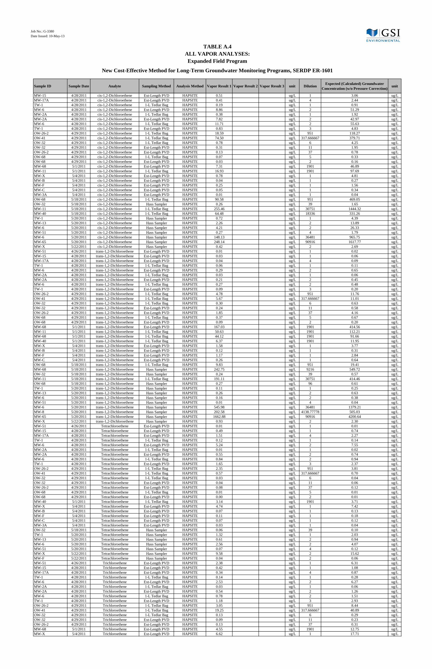
Job No.: G-3380Date Issued: 10-May-13
Sample ID Sample Date Analyte Sampling Method Analysis Method Vapor Result 1 Vapor Result 2 Vapor Result 3 unit Dilution Expected (Calculated) Groundwater Concentration (w/o Pressure Correction) unit
TABLE A.4ALL VAPOR ANALYSES:Expanded Field Program
New Cost-Effective Method for Long-Term Groundwater Monitoring Programs, SERDP ER-1601
MW-15 4/28/2011 cis-1,2-Dichloroethene Ext-Length PVD HAPSITE 0.51 ug/L 1 3.06 ug/LMW-17A 4/28/2011 cis-1,2-Dichloroethene Ext-Length PVD HAPSITE 0.41 ug/L 4 2.44 ug/LTW-1 4/28/2011 cis-1,2-Dichloroethene 1-L Tedlar Bag HAPSITE 0.19 ug/L 1 0.91 ug/LMW-6 4/28/2011 cis-1,2-Dichloroethene Ext-Length PVD HAPSITE 8.86 ug/L 2 51.29 ug/LMW-2A 4/28/2011 cis-1,2-Dichloroethene 1-L Tedlar Bag HAPSITE 0.38 ug/L 1 1.92 ug/LMW-2A 4/28/2011 cis-1,2-Dichloroethene Ext-Length PVD HAPSITE 7.82 ug/L 2 42.97 ug/LMW-6 4/28/2011 cis-1,2-Dichloroethene 1-L Tedlar Bag HAPSITE 11.71 ug/L 2 55.63 ug/LTW-1 4/28/2011 cis-1,2-Dichloroethene Ext-Length PVD HAPSITE 0.83 ug/L 3 4.83 ug/LOW-26-2 4/29/2011 cis-1,2-Dichloroethene 1-L Tedlar Bag HAPSITE 18.59 ug/L 951 118.27 ug/LOW-41 4/29/2011 cis-1,2-Dichloroethene 1-L Tedlar Bag HAPSITE 74.50 ug/L 317.666667 379.71 ug/LOW-32 4/29/2011 cis-1,2-Dichloroethene 1-L Tedlar Bag HAPSITE 0.78 ug/L 6 4.25 ug/LOW-32 4/29/2011 cis-1,2-Dichloroethene Ext-Length PVD HAPSITE 0.31 ug/L 11 1.95 ug/LOW-26-2 4/29/2011 cis-1,2-Dichloroethene Ext-Length PVD HAPSITE 0.13 ug/L 37 0.78 ug/LOW-68 4/29/2011 cis-1,2-Dichloroethene 1-L Tedlar Bag HAPSITE 0.07 ug/L 5 0.33 ug/LOW-68 4/29/2011 cis-1,2-Dichloroethene Ext-Length PVD HAPSITE 0.03 ug/L 2 0.16 ug/LMW-68 5/1/2011 cis-1,2-Dichloroethene Ext-Length PVD HAPSITE 7.31 ug/L 1901 46.89 ug/LMW-11 5/1/2011 cis-1,2-Dichloroethene 1-L Tedlar Bag HAPSITE 16.93 ug/L 1901 97.69 ug/LMW-X 5/4/2011 cis-1,2-Dichloroethene Ext-Length PVD HAPSITE 0.78 ug/L 1 4.81 ug/LMW-B 5/4/2011 cis-1,2-Dichloroethene Ext-Length PVD HAPSITE 0.04 ug/L 1 0.27 ug/LMW-F 5/4/2011 cis-1,2-Dichloroethene Ext-Length PVD HAPSITE 0.25 ug/L 1 1.56 ug/LMW-C 5/4/2011 cis-1,2-Dichloroethene Ext-Length PVD HAPSITE 0.05 ug/L 1 0.34 ug/LMW-3A 5/4/2011 cis-1,2-Dichloroethene Ext-Length PVD HAPSITE 0.01 ug/L 1 0.04 ug/LOW-68 5/18/2011 cis-1,2-Dichloroethene 1-L Tedlar Bag HAPSITE 90.58 ug/L 951 469.05 ug/LOW-32 5/18/2011 cis-1,2-Dichloroethene Hass Sampler HAPSITE 0.26 ug/L 39 1.65 ug/LMW-11 5/18/2011 cis-1,2-Dichloroethene 1-L Tedlar Bag HAPSITE 255.46 ug/L 30751 1444.32 ug/LMW-40 5/18/2011 cis-1,2-Dichloroethene 1-L Tedlar Bag HAPSITE 64.48 ug/L 18336 331.26 ug/LTW-1 5/20/2011 cis-1,2-Dichloroethene Hass Sampler HAPSITE 0.72 ug/L 1 4.39 ug/LMW-13 5/20/2011 cis-1,2-Dichloroethene Hass Sampler HAPSITE 2.26 ug/L 2 13.89 ug/LMW-6 5/20/2011 cis-1,2-Dichloroethene Hass Sampler HAPSITE 4.21 ug/L 2 26.33 ug/LMW-51 5/20/2011 cis-1,2-Dichloroethene Hass Sampler HAPSITE 0.27 ug/L 4 1.79 ug/LMW-6 5/20/2011 cis-1,2-Dichloroethene Hass Sampler HAPSITE 148.13 ug/L 36481 965.75 ug/LMW-65 5/20/2011 cis-1,2-Dichloroethene Hass Sampler HAPSITE 248.14 ug/L 90916 1617.77 ug/LMW-X 5/22/2011 cis-1,2-Dichloroethene Hass Sampler HAPSITE 0.42 ug/L 2 2.69 ug/LMW-51 4/26/2011 trans-1,2-Dichloroethene Ext-Length PVD HAPSITE 0.01 ug/L 1 0.02 ug/LMW-15 4/28/2011 trans-1,2-Dichloroethene Ext-Length PVD HAPSITE 0.03 ug/L 1 0.06 ug/LMW-17A 4/28/2011 trans-1,2-Dichloroethene Ext-Length PVD HAPSITE 0.04 ug/L 4 0.09 ug/LTW-1 4/28/2011 trans-1,2-Dichloroethene 1-L Tedlar Bag HAPSITE 0.06 ug/L 1 0.11 ug/LMW-6 4/28/2011 trans-1,2-Dichloroethene Ext-Length PVD HAPSITE 0.29 ug/L 2 0.65 ug/LMW-2A 4/28/2011 trans-1,2-Dichloroethene 1-L Tedlar Bag HAPSITE 0.03 ug/L 1 0.06 ug/LMW-2A 4/28/2011 trans-1,2-Dichloroethene Ext-Length PVD HAPSITE 0.21 ug/L 2 0.45 ug/LMW-6 4/28/2011 trans-1,2-Dichloroethene 1-L Tedlar Bag HAPSITE 0.27 ug/L 2 0.48 ug/LTW-1 4/28/2011 trans-1,2-Dichloroethene Ext-Length PVD HAPSITE 0.09 ug/L 3 0.20 ug/LOW-26-2 4/29/2011 trans-1,2-Dichloroethene 1-L Tedlar Bag HAPSITE 4.78 ug/L 951 11.76 ug/LOW-41 4/29/2011 trans-1,2-Dichloroethene 1-L Tedlar Bag HAPSITE 5.67 ug/L 317.666667 11.01 ug/LOW-32 4/29/2011 trans-1,2-Dichloroethene 1-L Tedlar Bag HAPSITE 0.30 ug/L 6 0.63 ug/LOW-32 4/29/2011 trans-1,2-Dichloroethene Ext-Length PVD HAPSITE 0.24 ug/L 11 0.58 ug/LOW-26-2 4/29/2011 trans-1,2-Dichloroethene Ext-Length PVD HAPSITE 1.85 ug/L 37 4.16 ug/LOW-68 4/29/2011 trans-1,2-Dichloroethene 1-L Tedlar Bag HAPSITE 0.37 ug/L 5 0.67 ug/LOW-68 4/29/2011 trans-1,2-Dichloroethene Ext-Length PVD HAPSITE 0.09 ug/L 2 0.20 ug/LMW-68 5/1/2011 trans-1,2-Dichloroethene Ext-Length PVD HAPSITE 167.03 ug/L 1901 414.56 ug/LMW-11 5/1/2011 trans-1,2-Dichloroethene 1-L Tedlar Bag HAPSITE 50.63 ug/L 1901 112.21 ug/LMW-68 5/1/2011 trans-1,2-Dichloroethene 1-L Tedlar Bag HAPSITE 44.12 ug/L 1901 91.66 ug/LMW-40 5/1/2011 trans-1,2-Dichloroethene 1-L Tedlar Bag HAPSITE 6.37 ug/L 1901 11.95 ug/LMW-X 5/4/2011 trans-1,2-Dichloroethene Ext-Length PVD HAPSITE 1.58 ug/L 1 3.77 ug/LMW-B 5/4/2011 trans-1,2-Dichloroethene Ext-Length PVD HAPSITE 0.12 ug/L 1 0.31 ug/LMW-F 5/4/2011 trans-1,2-Dichloroethene Ext-Length PVD HAPSITE 1.17 ug/L 1 2.84 ug/LMW-C 5/4/2011 trans-1,2-Dichloroethene Ext-Length PVD HAPSITE 0.26 ug/L 1 0.64 ug/LOW-68 5/18/2011 trans-1,2-Dichloroethene 1-L Tedlar Bag HAPSITE 9.83 ug/L 951 19.41 ug/LMW-68 5/18/2011 trans-1,2-Dichloroethene Hass Sampler HAPSITE 242.75 ug/L 9216 549.72 ug/LOW-32 5/18/2011 trans-1,2-Dichloroethene Hass Sampler HAPSITE 0.24 ug/L 39 0.57 ug/LMW-11 5/18/2011 trans-1,2-Dichloroethene 1-L Tedlar Bag HAPSITE 191.11 ug/L 30751 414.46 ug/LOW-68 5/18/2011 trans-1,2-Dichloroethene Hass Sampler HAPSITE 0.27 ug/L 96 0.61 ug/LTW-1 5/20/2011 trans-1,2-Dichloroethene Hass Sampler HAPSITE 0.11 ug/L 1 0.25 ug/LMW-13 5/20/2011 trans-1,2-Dichloroethene Hass Sampler HAPSITE 0.26 ug/L 2 0.63 ug/LMW-6 5/20/2011 trans-1,2-Dichloroethene Hass Sampler HAPSITE 0.16 ug/L 2 0.38 ug/LMW-51 5/20/2011 trans-1,2-Dichloroethene Hass Sampler HAPSITE 0.01 ug/L 4 0.04 ug/LMW-6 5/20/2011 trans-1,2-Dichloroethene Hass Sampler HAPSITE 545.98 ug/L 36481 1379.21 ug/LMW-8 5/20/2011 trans-1,2-Dichloroethene Hass Sampler HAPSITE 202.58 ug/L 4138.77778 505.03 ug/LMW-65 5/20/2011 trans-1,2-Dichloroethene Hass Sampler HAPSITE 1662.88 ug/L 90916 4200.64 ug/LMW-X 5/22/2011 trans-1,2-Dichloroethene Hass Sampler HAPSITE 0.93 ug/L 2 2.30 ug/LMW-51 4/26/2011 Tetrachloroethene Ext-Length PVD HAPSITE 0.01 ug/L 1 0.01 ug/LMW-15 4/28/2011 Tetrachloroethene Ext-Length PVD HAPSITE 0.49 ug/L 1 0.74 ug/LMW-17A 4/28/2011 Tetrachloroethene Ext-Length PVD HAPSITE 1.51 ug/L 4 2.27 ug/LTW-1 4/28/2011 Tetrachloroethene 1-L Tedlar Bag HAPSITE 0.12 ug/L 1 0.14 ug/LMW-6 4/28/2011 Tetrachloroethene Ext-Length PVD HAPSITE 5.24 ug/L 2 7.55 ug/LMW-2A 4/28/2011 Tetrachloroethene 1-L Tedlar Bag HAPSITE 0.01 ug/L 1 0.02 ug/LMW-2A 4/28/2011 Tetrachloroethene Ext-Length PVD HAPSITE 0.55 ug/L 2 0.74 ug/LMW-6 4/28/2011 Tetrachloroethene 1-L Tedlar Bag HAPSITE 0.84 ug/L 2 0.94 ug/LTW-1 4/28/2011 Tetrachloroethene Ext-Length PVD HAPSITE 1.65 ug/L 3 2.37 ug/LOW-26-2 4/29/2011 Tetrachloroethene 1-L Tedlar Bag HAPSITE 2.35 ug/L 951 3.81 ug/LOW-41 4/29/2011 Tetrachloroethene 1-L Tedlar Bag HAPSITE 0.57 ug/L 317.666667 0.70 ug/LOW-32 4/29/2011 Tetrachloroethene 1-L Tedlar Bag HAPSITE 0.03 ug/L 6 0.04 ug/LOW-32 4/29/2011 Tetrachloroethene Ext-Length PVD HAPSITE 0.04 ug/L 11 0.06 ug/LOW-26-2 4/29/2011 Tetrachloroethene Ext-Length PVD HAPSITE 0.08 ug/L 37 0.12 ug/LOW-68 4/29/2011 Tetrachloroethene 1-L Tedlar Bag HAPSITE 0.01 ug/L 5 0.01 ug/LOW-68 4/29/2011 Tetrachloroethene Ext-Length PVD HAPSITE 0.00 ug/L 2 0.01 ug/LMW-40 5/1/2011 Tetrachloroethene 1-L Tedlar Bag HAPSITE 3.14 ug/L 1901 3.71 ug/LMW-X 5/4/2011 Tetrachloroethene Ext-Length PVD HAPSITE 4.74 ug/L 1 7.42 ug/LMW-B 5/4/2011 Tetrachloroethene Ext-Length PVD HAPSITE 0.07 ug/L 1 0.13 ug/LMW-F 5/4/2011 Tetrachloroethene Ext-Length PVD HAPSITE 0.11 ug/L 1 0.18 ug/LMW-C 5/4/2011 Tetrachloroethene Ext-Length PVD HAPSITE 0.07 ug/L 1 0.12 ug/LMW-3A 5/4/2011 Tetrachloroethene Ext-Length PVD HAPSITE 0.03 ug/L 1 0.04 ug/LOW-32 5/18/2011 Tetrachloroethene Hass Sampler HAPSITE 0.06 ug/L 39 0.10 ug/LTW-1 5/20/2011 Tetrachloroethene Hass Sampler HAPSITE 1.32 ug/L 1 2.03 ug/LMW-13 5/20/2011 Tetrachloroethene Hass Sampler HAPSITE 0.61 ug/L 2 0.94 ug/LMW-6 5/20/2011 Tetrachloroethene Hass Sampler HAPSITE 2.56 ug/L 2 4.07 ug/LMW-51 5/20/2011 Tetrachloroethene Hass Sampler HAPSITE 0.07 ug/L 4 0.12 ug/LMW-X 5/22/2011 Tetrachloroethene Hass Sampler HAPSITE 9.58 ug/L 2 15.62 ug/LMW-F 5/22/2011 Tetrachloroethene Hass Sampler HAPSITE 0.04 ug/L 2 0.06 ug/LMW-51 4/26/2011 Trichloroethene Ext-Length PVD HAPSITE 2.38 ug/L 1 6.31 ug/LMW-15 4/28/2011 Trichloroethene Ext-Length PVD HAPSITE 0.42 ug/L 1 1.08 ug/LMW-17A 4/28/2011 Trichloroethene Ext-Length PVD HAPSITE 0.34 ug/L 4 0.87 ug/LTW-1 4/28/2011 Trichloroethene 1-L Tedlar Bag HAPSITE 0.14 ug/L 1 0.28 ug/LMW-6 4/28/2011 Trichloroethene Ext-Length PVD HAPSITE 2.53 ug/L 2 6.27 ug/LMW-2A 4/28/2011 Trichloroethene 1-L Tedlar Bag HAPSITE 0.03 ug/L 1 0.06 ug/LMW-2A 4/28/2011 Trichloroethene Ext-Length PVD HAPSITE 0.54 ug/L 2 1.26 ug/LMW-6 4/28/2011 Trichloroethene 1-L Tedlar Bag HAPSITE 0.78 ug/L 2 1.51 ug/LTW-1 4/28/2011 Trichloroethene Ext-Length PVD HAPSITE 1.18 ug/L 3 2.93 ug/LOW-26-2 4/29/2011 Trichloroethene 1-L Tedlar Bag HAPSITE 3.05 ug/L 951 8.44 ug/LOW-41 4/29/2011 Trichloroethene 1-L Tedlar Bag HAPSITE 19.25 ug/L 317.666667 40.89 ug/LOW-32 4/29/2011 Trichloroethene 1-L Tedlar Bag HAPSITE 0.13 ug/L 6 0.29 ug/LOW-32 4/29/2011 Trichloroethene Ext-Length PVD HAPSITE 0.09 ug/L 11 0.23 ug/LOW-26-2 4/29/2011 Trichloroethene Ext-Length PVD HAPSITE 0.13 ug/L 37 0.31 ug/LMW-68 5/1/2011 Trichloroethene Ext-Length PVD HAPSITE 4.55 ug/L 1901 12.75 ug/LMW-X 5/4/2011 Trichloroethene Ext-Length PVD HAPSITE 6.62 ug/L 1 17.71 ug/L
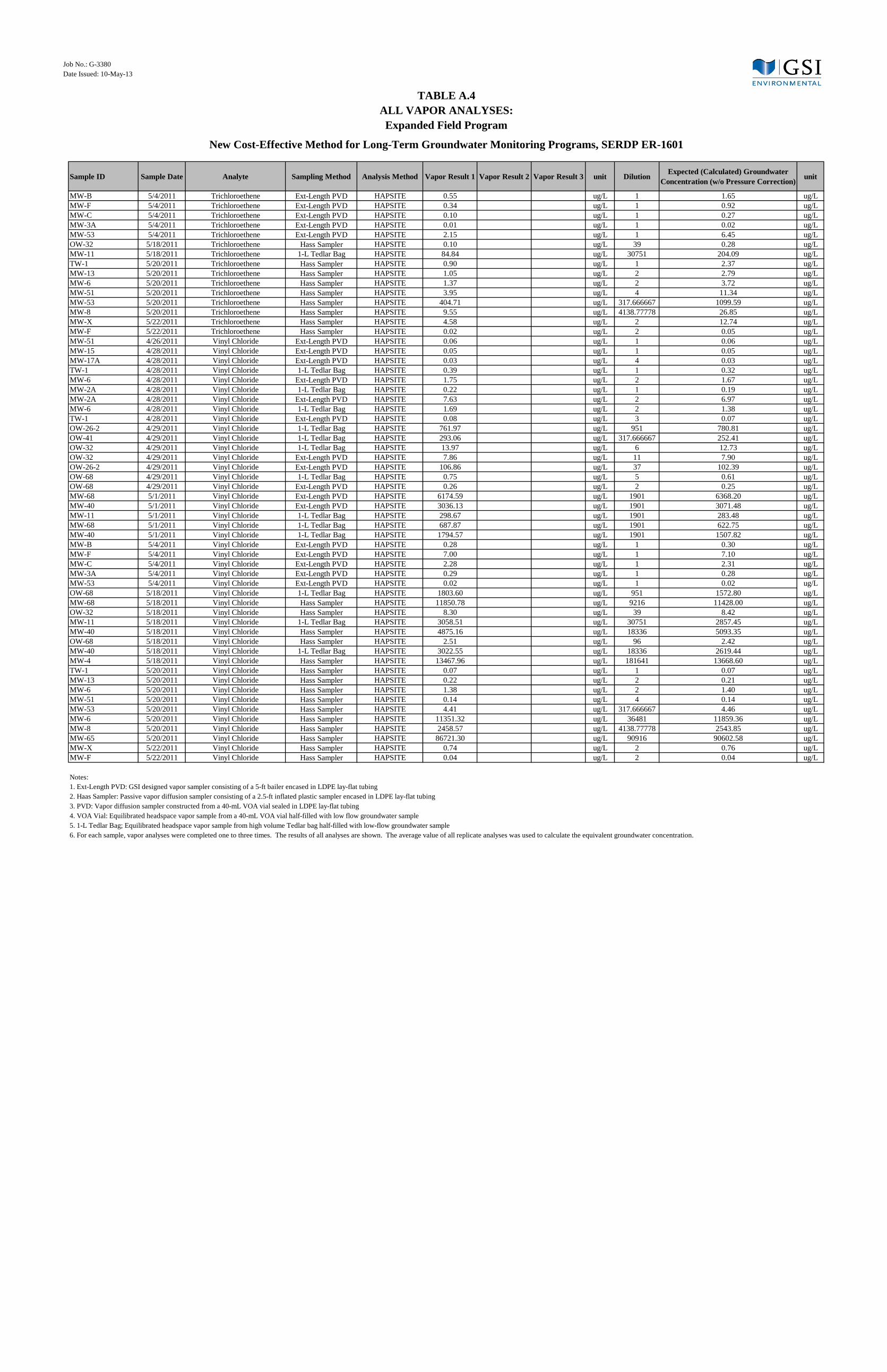
Job No.: G-3380Date Issued: 10-May-13
Sample ID Sample Date Analyte Sampling Method Analysis Method Vapor Result 1 Vapor Result 2 Vapor Result 3 unit Dilution Expected (Calculated) Groundwater Concentration (w/o Pressure Correction) unit
TABLE A.4ALL VAPOR ANALYSES:Expanded Field Program
New Cost-Effective Method for Long-Term Groundwater Monitoring Programs, SERDP ER-1601
MW-B 5/4/2011 Trichloroethene Ext-Length PVD HAPSITE 0.55 ug/L 1 1.65 ug/LMW-F 5/4/2011 Trichloroethene Ext-Length PVD HAPSITE 0.34 ug/L 1 0.92 ug/LMW-C 5/4/2011 Trichloroethene Ext-Length PVD HAPSITE 0.10 ug/L 1 0.27 ug/LMW-3A 5/4/2011 Trichloroethene Ext-Length PVD HAPSITE 0.01 ug/L 1 0.02 ug/LMW-53 5/4/2011 Trichloroethene Ext-Length PVD HAPSITE 2.15 ug/L 1 6.45 ug/LOW-32 5/18/2011 Trichloroethene Hass Sampler HAPSITE 0.10 ug/L 39 0.28 ug/LMW-11 5/18/2011 Trichloroethene 1-L Tedlar Bag HAPSITE 84.84 ug/L 30751 204.09 ug/LTW-1 5/20/2011 Trichloroethene Hass Sampler HAPSITE 0.90 ug/L 1 2.37 ug/LMW-13 5/20/2011 Trichloroethene Hass Sampler HAPSITE 1.05 ug/L 2 2.79 ug/LMW-6 5/20/2011 Trichloroethene Hass Sampler HAPSITE 1.37 ug/L 2 3.72 ug/LMW-51 5/20/2011 Trichloroethene Hass Sampler HAPSITE 3.95 ug/L 4 11.34 ug/LMW-53 5/20/2011 Trichloroethene Hass Sampler HAPSITE 404.71 ug/L 317.666667 1099.59 ug/LMW-8 5/20/2011 Trichloroethene Hass Sampler HAPSITE 9.55 ug/L 4138.77778 26.85 ug/LMW-X 5/22/2011 Trichloroethene Hass Sampler HAPSITE 4.58 ug/L 2 12.74 ug/LMW-F 5/22/2011 Trichloroethene Hass Sampler HAPSITE 0.02 ug/L 2 0.05 ug/LMW-51 4/26/2011 Vinyl Chloride Ext-Length PVD HAPSITE 0.06 ug/L 1 0.06 ug/LMW-15 4/28/2011 Vinyl Chloride Ext-Length PVD HAPSITE 0.05 ug/L 1 0.05 ug/LMW-17A 4/28/2011 Vinyl Chloride Ext-Length PVD HAPSITE 0.03 ug/L 4 0.03 ug/LTW-1 4/28/2011 Vinyl Chloride 1-L Tedlar Bag HAPSITE 0.39 ug/L 1 0.32 ug/LMW-6 4/28/2011 Vinyl Chloride Ext-Length PVD HAPSITE 1.75 ug/L 2 1.67 ug/LMW-2A 4/28/2011 Vinyl Chloride 1-L Tedlar Bag HAPSITE 0.22 ug/L 1 0.19 ug/LMW-2A 4/28/2011 Vinyl Chloride Ext-Length PVD HAPSITE 7.63 ug/L 2 6.97 ug/LMW-6 4/28/2011 Vinyl Chloride 1-L Tedlar Bag HAPSITE 1.69 ug/L 2 1.38 ug/LTW-1 4/28/2011 Vinyl Chloride Ext-Length PVD HAPSITE 0.08 ug/L 3 0.07 ug/LOW-26-2 4/29/2011 Vinyl Chloride 1-L Tedlar Bag HAPSITE 761.97 ug/L 951 780.81 ug/LOW-41 4/29/2011 Vinyl Chloride 1-L Tedlar Bag HAPSITE 293.06 ug/L 317.666667 252.41 ug/LOW-32 4/29/2011 Vinyl Chloride 1-L Tedlar Bag HAPSITE 13.97 ug/L 6 12.73 ug/LOW-32 4/29/2011 Vinyl Chloride Ext-Length PVD HAPSITE 7.86 ug/L 11 7.90 ug/LOW-26-2 4/29/2011 Vinyl Chloride Ext-Length PVD HAPSITE 106.86 ug/L 37 102.39 ug/LOW-68 4/29/2011 Vinyl Chloride 1-L Tedlar Bag HAPSITE 0.75 ug/L 5 0.61 ug/LOW-68 4/29/2011 Vinyl Chloride Ext-Length PVD HAPSITE 0.26 ug/L 2 0.25 ug/LMW-68 5/1/2011 Vinyl Chloride Ext-Length PVD HAPSITE 6174.59 ug/L 1901 6368.20 ug/LMW-40 5/1/2011 Vinyl Chloride Ext-Length PVD HAPSITE 3036.13 ug/L 1901 3071.48 ug/LMW-11 5/1/2011 Vinyl Chloride 1-L Tedlar Bag HAPSITE 298.67 ug/L 1901 283.48 ug/LMW-68 5/1/2011 Vinyl Chloride 1-L Tedlar Bag HAPSITE 687.87 ug/L 1901 622.75 ug/LMW-40 5/1/2011 Vinyl Chloride 1-L Tedlar Bag HAPSITE 1794.57 ug/L 1901 1507.82 ug/LMW-B 5/4/2011 Vinyl Chloride Ext-Length PVD HAPSITE 0.28 ug/L 1 0.30 ug/LMW-F 5/4/2011 Vinyl Chloride Ext-Length PVD HAPSITE 7.00 ug/L 1 7.10 ug/LMW-C 5/4/2011 Vinyl Chloride Ext-Length PVD HAPSITE 2.28 ug/L 1 2.31 ug/LMW-3A 5/4/2011 Vinyl Chloride Ext-Length PVD HAPSITE 0.29 ug/L 1 0.28 ug/LMW-53 5/4/2011 Vinyl Chloride Ext-Length PVD HAPSITE 0.02 ug/L 1 0.02 ug/LOW-68 5/18/2011 Vinyl Chloride 1-L Tedlar Bag HAPSITE 1803.60 ug/L 951 1572.80 ug/LMW-68 5/18/2011 Vinyl Chloride Hass Sampler HAPSITE 11850.78 ug/L 9216 11428.00 ug/LOW-32 5/18/2011 Vinyl Chloride Hass Sampler HAPSITE 8.30 ug/L 39 8.42 ug/LMW-11 5/18/2011 Vinyl Chloride 1-L Tedlar Bag HAPSITE 3058.51 ug/L 30751 2857.45 ug/LMW-40 5/18/2011 Vinyl Chloride Hass Sampler HAPSITE 4875.16 ug/L 18336 5093.35 ug/LOW-68 5/18/2011 Vinyl Chloride Hass Sampler HAPSITE 2.51 ug/L 96 2.42 ug/LMW-40 5/18/2011 Vinyl Chloride 1-L Tedlar Bag HAPSITE 3022.55 ug/L 18336 2619.44 ug/LMW-4 5/18/2011 Vinyl Chloride Hass Sampler HAPSITE 13467.96 ug/L 181641 13668.60 ug/LTW-1 5/20/2011 Vinyl Chloride Hass Sampler HAPSITE 0.07 ug/L 1 0.07 ug/LMW-13 5/20/2011 Vinyl Chloride Hass Sampler HAPSITE 0.22 ug/L 2 0.21 ug/LMW-6 5/20/2011 Vinyl Chloride Hass Sampler HAPSITE 1.38 ug/L 2 1.40 ug/LMW-51 5/20/2011 Vinyl Chloride Hass Sampler HAPSITE 0.14 ug/L 4 0.14 ug/LMW-53 5/20/2011 Vinyl Chloride Hass Sampler HAPSITE 4.41 ug/L 317.666667 4.46 ug/LMW-6 5/20/2011 Vinyl Chloride Hass Sampler HAPSITE 11351.32 ug/L 36481 11859.36 ug/LMW-8 5/20/2011 Vinyl Chloride Hass Sampler HAPSITE 2458.57 ug/L 4138.77778 2543.85 ug/LMW-65 5/20/2011 Vinyl Chloride Hass Sampler HAPSITE 86721.30 ug/L 90916 90602.58 ug/LMW-X 5/22/2011 Vinyl Chloride Hass Sampler HAPSITE 0.74 ug/L 2 0.76 ug/LMW-F 5/22/2011 Vinyl Chloride Hass Sampler HAPSITE 0.04 ug/L 2 0.04 ug/L
Notes:1. Ext-Length PVD: GSI designed vapor sampler consisting of a 5-ft bailer encased in LDPE lay-flat tubing2. Haas Sampler: Passive vapor diffusion sampler consisting of a 2.5-ft inflated plastic sampler encased in LDPE lay-flat tubing3. PVD: Vapor diffusion sampler constructed from a 40-mL VOA vial sealed in LDPE lay-flat tubing4. VOA Vial: Equilibrated headspace vapor sample from a 40-mL VOA vial half-filled with low flow groundwater sample5. 1-L Tedlar Bag; Equilibrated headspace vapor sample from high volume Tedlar bag half-filled with low-flow groundwater sample6. For each sample, vapor analyses were completed one to three times. The results of all analyses are shown. The average value of all replicate analyses was used to calculate the equivalent groundwater concentration.
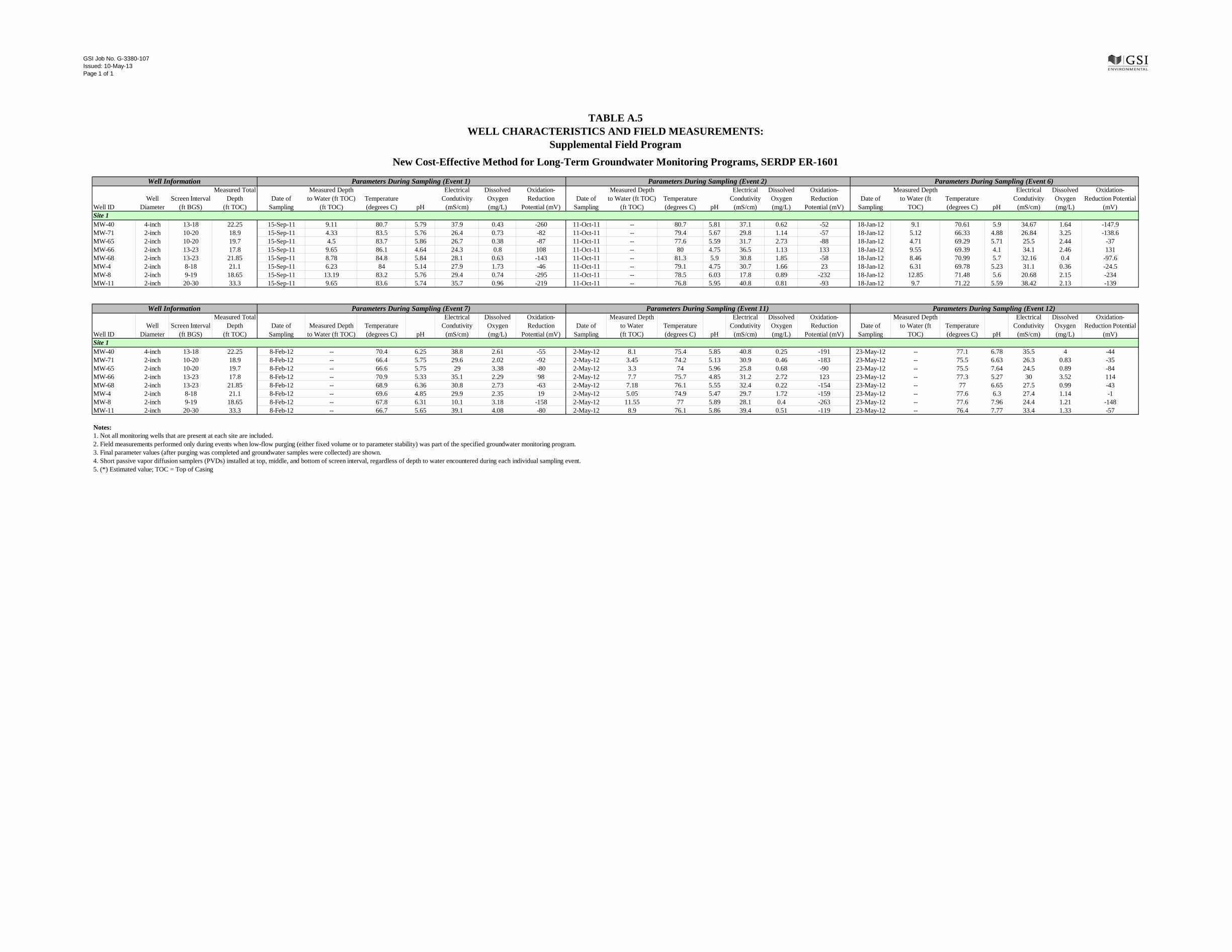
GSI Job No. G-3380-107Issued: 10-May-13Page 1 of 1
Well IDWell
DiameterScreen Interval
(ft BGS)
Measured Total Depth
(ft TOC)Date of
Sampling
Measured Depth to Water (ft TOC)
(ft TOC)Temperature (degrees C) pH
Electrical Condutivity
(mS/cm)
Dissolved Oxygen (mg/L)
Oxidation-Reduction
Potential (mV)Date of
Sampling
Measured Depth to Water (ft TOC)
(ft TOC)Temperature (degrees C) pH
Electrical Condutivity
(mS/cm)
Dissolved Oxygen (mg/L)
Oxidation-Reduction
Potential (mV)Date of
Sampling
Measured Depth to Water (ft
TOC)Temperature (degrees C) pH
Electrical Condutivity
(mS/cm)
Dissolved Oxygen (mg/L)
Oxidation-Reduction Potential
(mV)
MW-40 4-inch 13-18 22.25 15-Sep-11 9.11 80.7 5.79 37.9 0.43 -260 11-Oct-11 -- 80.7 5.81 37.1 0.62 -52 18-Jan-12 9.1 70.61 5.9 34.67 1.64 -147.9MW-71 2-inch 10-20 18.9 15-Sep-11 4.33 83.5 5.76 26.4 0.73 -82 11-Oct-11 -- 79.4 5.67 29.8 1.14 -57 18-Jan-12 5.12 66.33 4.88 26.84 3.25 -138.6MW-65 2-inch 10-20 19.7 15-Sep-11 4.5 83.7 5.86 26.7 0.38 -87 11-Oct-11 -- 77.6 5.59 31.7 2.73 -88 18-Jan-12 4.71 69.29 5.71 25.5 2.44 -37MW-66 2-inch 13-23 17.8 15-Sep-11 9.65 86.1 4.64 24.3 0.8 108 11-Oct-11 -- 80 4.75 36.5 1.13 133 18-Jan-12 9.55 69.39 4.1 34.1 2.46 131MW-68 2-inch 13-23 21.85 15-Sep-11 8.78 84.8 5.84 28.1 0.63 -143 11-Oct-11 -- 81.3 5.9 30.8 1.85 -58 18-Jan-12 8.46 70.99 5.7 32.16 0.4 -97.6MW-4 2-inch 8-18 21.1 15-Sep-11 6.23 84 5.14 27.9 1.73 -46 11-Oct-11 -- 79.1 4.75 30.7 1.66 23 18-Jan-12 6.31 69.78 5.23 31.1 0.36 -24.5MW-8 2-inch 9-19 18.65 15-Sep-11 13.19 83.2 5.76 29.4 0.74 -295 11-Oct-11 -- 78.5 6.03 17.8 0.89 -232 18-Jan-12 12.85 71.48 5.6 20.68 2.15 -234MW-11 2-inch 20-30 33.3 15-Sep-11 9.65 83.6 5.74 35.7 0.96 -219 11-Oct-11 -- 76.8 5.95 40.8 0.81 -93 18-Jan-12 9.7 71.22 5.59 38.42 2.13 -139
Well IDWell
DiameterScreen Interval
(ft BGS)
Measured Total Depth
(ft TOC)Date of
SamplingMeasured Depth
to Water (ft TOC)Temperature (degrees C) pH
Electrical Condutivity
(mS/cm)
Dissolved Oxygen (mg/L)
Oxidation-Reduction
Potential (mV)Date of
Sampling
Measured Depth to Water(ft TOC)
Temperature (degrees C) pH
Electrical Condutivity
(mS/cm)
Dissolved Oxygen (mg/L)
Oxidation-Reduction
Potential (mV)Date of
Sampling
Measured Depth to Water (ft
TOC)Temperature (degrees C) pH
Electrical Condutivity
(mS/cm)
Dissolved Oxygen (mg/L)
Oxidation-Reduction Potential
(mV)
MW-40 4-inch 13-18 22.25 8-Feb-12 -- 70.4 6.25 38.8 2.61 -55 2-May-12 8.1 75.4 5.85 40.8 0.25 -191 23-May-12 -- 77.1 6.78 35.5 4 -44MW-71 2-inch 10-20 18.9 8-Feb-12 -- 66.4 5.75 29.6 2.02 -92 2-May-12 3.45 74.2 5.13 30.9 0.46 -183 23-May-12 -- 75.5 6.63 26.3 0.83 -35MW-65 2-inch 10-20 19.7 8-Feb-12 -- 66.6 5.75 29 3.38 -80 2-May-12 3.3 74 5.96 25.8 0.68 -90 23-May-12 -- 75.5 7.64 24.5 0.89 -84MW-66 2-inch 13-23 17.8 8-Feb-12 -- 70.9 5.33 35.1 2.29 98 2-May-12 7.7 75.7 4.85 31.2 2.72 123 23-May-12 -- 77.3 5.27 30 3.52 114MW-68 2-inch 13-23 21.85 8-Feb-12 -- 68.9 6.36 30.8 2.73 -63 2-May-12 7.18 76.1 5.55 32.4 0.22 -154 23-May-12 -- 77 6.65 27.5 0.99 -43MW-4 2-inch 8-18 21.1 8-Feb-12 -- 69.6 4.85 29.9 2.35 19 2-May-12 5.05 74.9 5.47 29.7 1.72 -159 23-May-12 -- 77.6 6.3 27.4 1.14 -1MW-8 2-inch 9-19 18.65 8-Feb-12 -- 67.8 6.31 10.1 3.18 -158 2-May-12 11.55 77 5.89 28.1 0.4 -263 23-May-12 -- 77.6 7.96 24.4 1.21 -148MW-11 2-inch 20-30 33.3 8-Feb-12 -- 66.7 5.65 39.1 4.08 -80 2-May-12 8.9 76.1 5.86 39.4 0.51 -119 23-May-12 -- 76.4 7.77 33.4 1.33 -57
Notes:1. Not all monitoring wells that are present at each site are included.2. Field measurements performed only during events when low-flow purging (either fixed volume or to parameter stability) was part of the specified groundwater monitoring program.3. Final parameter values (after purging was completed and groundwater samples were collected) are shown.4. Short passive vapor diffusion samplers (PVDs) installed at top, middle, and bottom of screen interval, regardless of depth to water encountered during each individual sampling event.5. (*) Estimated value; TOC = Top of Casing
Site 1
Parameters During Sampling (Event 6)Parameters During Sampling (Event 1) Parameters During Sampling (Event 2)
Parameters During Sampling (Event 12)
TABLE A.5WELL CHARACTERISTICS AND FIELD MEASUREMENTS:
Supplemental Field Program
Site 1
Well Information
Well Information
New Cost-Effective Method for Long-Term Groundwater Monitoring Programs, SERDP ER-1601
Parameters During Sampling (Event 7) Parameters During Sampling (Event 11)
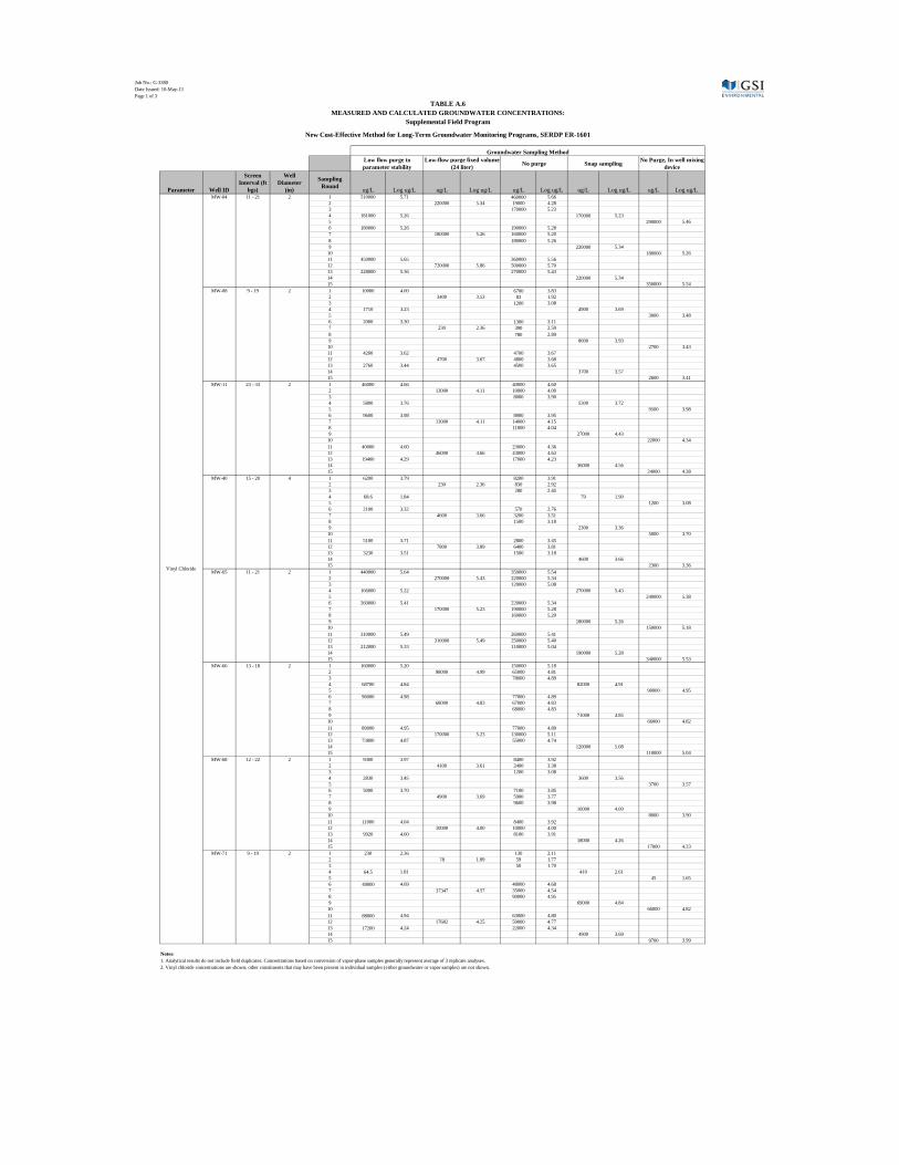
Job No.: G-3380Date Issued: 10-May-13Page 1 of 3
Parameter Well ID
Screen Interval (ft
bgs)
Well Diameter
(in)
Sampling Round ug/L Log ug/L ug/L Log ug/L ug/L Log ug/L ug/L Log ug/L ug/L Log ug/L
1 510000 5.71 460000 5.662 220000 5.34 19000 4.283 170000 5.234 181000 5.26 170000 5.235 290000 5.466 180000 5.26 190000 5.287 180000 5.26 160000 5.208 180000 5.269 220000 5.3410 180000 5.2611 450000 5.65 360000 5.5612 720000 5.86 500000 5.7013 228000 5.36 270000 5.4314 220000 5.3415 350000 5.541 10000 4.00 6700 3.832 3400 3.53 83 1.923 1200 3.084 1710 3.23 4900 3.695 3000 3.486 2000 3.30 1300 3.117 230 2.36 390 2.598 780 2.899 8600 3.9310 2700 3.4311 4200 3.62 4700 3.6712 4700 3.67 4800 3.6813 2760 3.44 4500 3.6514 3700 3.5715 2600 3.411 46000 4.66 40000 4.602 13000 4.11 10000 4.003 8000 3.904 5800 3.76 5300 3.725 9500 3.986 9600 3.98 8900 3.957 13000 4.11 14000 4.158 11000 4.049 27000 4.4310 22000 4.3411 40000 4.60 23000 4.3612 46000 4.66 43000 4.6313 19400 4.29 17000 4.2314 36000 4.5615 24000 4.381 6200 3.79 8200 3.912 230 2.36 830 2.923 280 2.454 68.6 1.84 79 1.905 1200 3.086 2100 3.32 570 2.767 4600 3.66 3200 3.518 1500 3.189 2300 3.3610 5000 3.7011 5100 3.71 2800 3.4512 7800 3.89 6400 3.8113 3230 3.51 1500 3.1814 4600 3.6615 2300 3.361 440000 5.64 350000 5.542 270000 5.43 220000 5.343 120000 5.084 166000 5.22 270000 5.435 240000 5.386 260000 5.41 220000 5.347 170000 5.23 190000 5.288 160000 5.209 180000 5.2610 150000 5.1811 310000 5.49 260000 5.4112 310000 5.49 250000 5.4013 212000 5.33 110000 5.0414 190000 5.2815 340000 5.531 160000 5.20 150000 5.182 98000 4.99 65000 4.813 78000 4.894 68700 4.84 82000 4.915 90000 4.956 96000 4.98 77000 4.897 68000 4.83 67000 4.838 68000 4.839 71000 4.8510 66000 4.8211 89000 4.95 77000 4.8912 170000 5.23 130000 5.1113 73800 4.87 55000 4.7414 120000 5.0815 110000 5.041 9300 3.97 8400 3.922 4100 3.61 2400 3.383 1200 3.084 2830 3.45 3600 3.565 3700 3.576 5000 3.70 7100 3.857 4900 3.69 5900 3.778 9600 3.989 10000 4.0010 8000 3.9011 11000 4.04 8400 3.9212 10000 4.00 10000 4.0013 9920 4.00 8100 3.9114 18000 4.2615 17000 4.231 230 2.36 130 2.112 78 1.89 59 1.773 50 1.704 64.5 1.81 410 2.615 45 1.656 49000 4.69 48000 4.687 37347 4.57 35000 4.548 90000 4.959 69000 4.8410 66000 4.8211 88000 4.94 63000 4.8012 17682 4.25 59000 4.7713 17200 4.24 22000 4.3414 4900 3.6915 9700 3.99
Notes:1. Analytical results do not include field duplicates. Concentrations based on conversion of vapor-phase samples generally represent average of 3 replicate analyses.2. Vinyl chloride concentrations are shown; other constituents that may have been present in individual samples (either groundwater or vapor samples) are not shown.
Groundwater Sampling Method
MW-66 13 - 18 2
MW-68 12 - 22 2
23 - 33 2
MW-40 15 - 20 4
Vinyl Chloride
MW-04 11 - 21 2
MW-08 9 - 19 2
MW-11
MW-65 11 - 21 2
MW-71 9 - 19 2
Low flow purge to parameter stability
Low-flow purge fixed volume (24 liter) No purge Snap sampling No Purge, In well mixing
device
TABLE A.6MEASURED AND CALCULATED GROUNDWATER CONCENTRATIONS:
Supplemental Field Program
New Cost-Effective Method for Long-Term Groundwater Monitoring Programs, SERDP ER-1601

Job No.: G-3380Date Issued: 10-May-13Page 2 of 3
Parameter Well ID
Screen Interval (ft
bgs)
Well Diameter
(in)
Sampling Round ug/L
Pressure Corrected Log ug/L ug/L
Pressure Corrected Log ug/L ug/L
Pressure Corrected Log ug/L
Pressure Corrected Log ug/L
12 565089 617298 5.79 496587 600975 5.78 473738 629139 5.80 615804 5.793 489025 534206 5.73 347556 420616 5.62 207064 274987 5.44 409937 5.614 637683 696599 5.84 653113 790405 5.90 581893 772772 5.89 753259 5.8856 581208 634906 5.80 703316 851161 5.93 210463 279501 5.45 588523 5.777 554888 606155 5.78 674863 816727 5.91 623389 827880 5.92 750254 5.888 886480 968383 5.99 889978 1077061 6.03 830500 1102930 6.04 1049458 6.029 542817 592968 5.77 523337 633348 5.80 498195 661619 5.82 629312 5.801011 668483 730245 5.86 633876 767124 5.88 556927 739617 5.87 745662 5.8712 762957 833447 5.92 778484 942130 5.97 685425 910266 5.96 895281 5.9513 721771 788456 5.90 727829 880827 5.94 671581 891881 5.95 853721 5.9314 635491 694205 5.84 595724 720952 5.86 531027 705221 5.85 706792 5.851512 14375 14375 4.16 4148 4328 3.64 5816 6753 3.83 8485 3.933 3318 3318 3.52 66 69 1.84 898 1043 3.02 1477 3.174 8495 8495 3.93 1961 2046 3.31 8555 9933 4.00 6825 3.8356 2712 2712 3.43 1220 1273 3.10 4231 4913 3.69 2966 3.477 511 511 2.71 482 503 2.70 2596 3014 3.48 1343 3.138 2620 2620 3.42 1966 2051 3.31 2739 3180 3.50 2617 3.429 4625 4625 3.67 1880 1961 3.29 877 1018 3.01 2535 3.401011 10680 10680 4.03 2711 2828 3.45 1479 1717 3.23 5075 3.7112 19274 19274 4.28 6921 7221 3.86 1860 2160 3.33 9551 3.9813 20705 20705 4.32 504 526 2.72 2779 3227 3.51 8153 3.9114 20563 20563 4.31 1288 1344 3.13 1571 1824 3.26 7910 3.901512 40327 54082 4.73 39309 57348 4.76 41338 65179 4.81 58870 4.773 40609 54460 4.74 40156 58584 4.77 42233 66590 4.82 59878 4.784 26104 35008 4.54 18321 26729 4.43 8814 13897 4.14 25211 4.4056 7042 9444 3.98 14931 21783 4.34 5506 8681 3.94 13303 4.127 10514 14100 4.15 21579 31482 4.50 23028 36309 4.56 27297 4.448 28142 37741 4.58 58229 84951 4.93 23737 37427 4.57 53373 4.739 10942 14674 4.17 50056 73027 4.86 22429 35364 4.55 41022 4.611011 42798 57396 4.76 56397 82278 4.92 54704 86253 4.94 75309 4.8812 77602 104071 5.02 48696 71043 4.85 78376 123578 5.09 99564 5.0013 27621 37042 4.57 64930 94727 4.98 54492 85919 4.93 72563 4.8614 36146 48475 4.69 57912 84488 4.93 24725 38985 4.59 57316 4.761512 3260 3762 3.58 2537 3040 3.48 9884 12280 4.09 6361 3.803 271 313 2.50 62 74 1.87 51 63 1.80 150 2.184 261 301 2.48 306 367 2.56 156 194 2.29 287 2.4656 12 14 1.14 31 37 1.57 4 5 0.70 19 1.277 621 717 2.86 675 809 2.91 4852 6028 3.78 2518 3.408 1663 1919 3.28 3349 4013 3.60 33038 41047 4.61 15660 4.199 944 1089 3.04 6943 8319 3.92 7943 9869 3.99 6426 3.811011 2699 3115 3.49 10394 12454 4.10 11830 14698 4.17 10089 4.0012 2967 3424 3.53 9499 11382 4.06 16219 20151 4.30 11652 4.0713 4570 5274 3.72 10133 12142 4.08 11407 14172 4.15 10529 4.0214 4937 5698 3.76 7834 9387 3.97 6749 8385 3.92 7823 3.891512 421512 506311 5.70 504990 666081 5.82 460310 661382 5.82 611258 5.793 516019 619831 5.79 728451 960826 5.98 684822 983965 5.99 854874 5.934 641934 771077 5.89 462260 609720 5.79 534897 768550 5.89 716449 5.8656 348595 418725 5.62 508389 670564 5.83 613348 881270 5.95 656853 5.827 477129 573117 5.76 559517 738002 5.87 673441 967613 5.99 759577 5.888 503310 604565 5.78 858886 1132869 6.05 875370 1257748 6.10 998394 6.009 375944 451576 5.65 368705 486321 5.69 491661 706428 5.85 548108 5.741011 388888 467124 5.67 328702 433557 5.64 582225 836552 5.92 579078 5.7612 430526 517138 5.71 522917 689727 5.84 645770 927855 5.97 711573 5.8513 440667 529320 5.72 474342 625656 5.80 480500 690391 5.84 615122 5.7914 449833 540330 5.73 484108 638538 5.81 445994 640813 5.81 606560 5.781512 210100 241249 5.38 210053 265943 5.42 210084 290735 5.46 265976 5.423 136800 157082 5.20 97623 123598 5.09 11889 16453 4.22 99044 5.004 228407 262270 5.42 274281 347261 5.54 246825 341581 5.53 317037 5.5056 91157 104672 5.02 158961 201257 5.30 176729 244575 5.39 183501 5.267 225089 258460 5.41 201423 255017 5.41 225602 312210 5.49 275229 5.448 241942 277812 5.44 354701 449079 5.65 429486 594365 5.77 440418 5.649 100583 115495 5.06 185479 234831 5.37 198135 274199 5.44 208175 5.321011 144993 166489 5.22 160585 203313 5.31 260078 359921 5.56 243241 5.3912 161949 185959 5.27 234698 297146 5.47 263558 364737 5.56 282614 5.4513 167041 191806 5.28 175627 222357 5.35 235405 325776 5.51 246647 5.3914 158997 182569 5.26 181986 230408 5.36 229611 317758 5.50 243579 5.391512 4844 5680 3.75 3620 4671 3.67 3593 5060 3.70 5137 3.713 8644 10136 4.01 4943 6379 3.80 7698 10841 4.04 9118 3.964 10640 12477 4.10 11431 14751 4.17 10378 14615 4.16 13947 4.1456 12613 14790 4.17 9415 12149 4.08 10976 15457 4.19 14132 4.157 10562 12385 4.09 5482 7074 3.85 5457 7685 3.89 9048 3.968 61797 72464 4.86 55134 71146 4.85 49832 70176 4.85 71262 4.859 20752 24334 4.39 21380 27589 4.44 22730 32009 4.51 27978 4.451011 27631 32400 4.51 25196 32514 4.51 25897 36469 4.56 33794 4.5312 11790 13825 4.14 19392 25024 4.40 27656 38946 4.59 25932 4.4113 30655 35946 4.56 25308 32658 4.51 30933 43561 4.64 37389 4.5714 23381 27417 4.44 8635 11143 4.05 11395 16047 4.21 18202 4.261512 5888 7050 3.85 6347 8347 3.92 5109 7321 3.86 7573 3.883 2948 3530 3.55 5585 7345 3.87 4046 5798 3.76 5558 3.744 4974 5956 3.77 396 521 2.72 6053 8674 3.94 5050 3.7056 67439 80748 4.91 72446 95279 4.98 70024 100344 5.00 92123 4.967 36970 44266 4.65 42348 55695 4.75 67663 96960 4.99 65640 4.828 210967 252601 5.40 207867 273380 5.44 204062 292419 5.47 272800 5.449 92585 110857 5.04 97507 128238 5.11 87470 125344 5.10 121479 5.081011 148598 177924 5.25 148993 195951 5.29 148479 212769 5.33 195548 5.2912 97709 116992 5.07 97378 128069 5.11 17125 24540 4.39 89867 4.9513 57596 68963 4.84 55278 72700 4.86 56756 81331 4.91 74331 4.8714 24830 29730 4.47 25220 33169 4.52 18566 26605 4.42 29835 4.4715
Notes:1. Analytical results do not include field duplicates. Concentrations based on conversion of vapor-phase samples generally represent average of 3 replicate analyses.2. Vinyl chloride concentrations are shown; other constituents that may have been present in individual samples (either groundwater or vapor samples) are not shown.
PVD Top PVD Middle PVD Bottom PVD Average
13 - 18 2
Vinyl Chloride
MW-04 11 - 21 2
MW-08 9 - 19 2
MW-11 23 - 33 2
MW-40 15 - 20 4
2
MW-65 11 - 21 2
MW-66
Vapor-Based Sampling Method
TABLE A.6MEASURED AND CALCULATED GROUNDWATER CONCENTRATIONS:
Supplemental Field Program
New Cost-Effective Method for Long-Term Groundwater Monitoring Programs, SERDP ER-1601
MW-68 12 - 22 2
MW-71 9 - 19
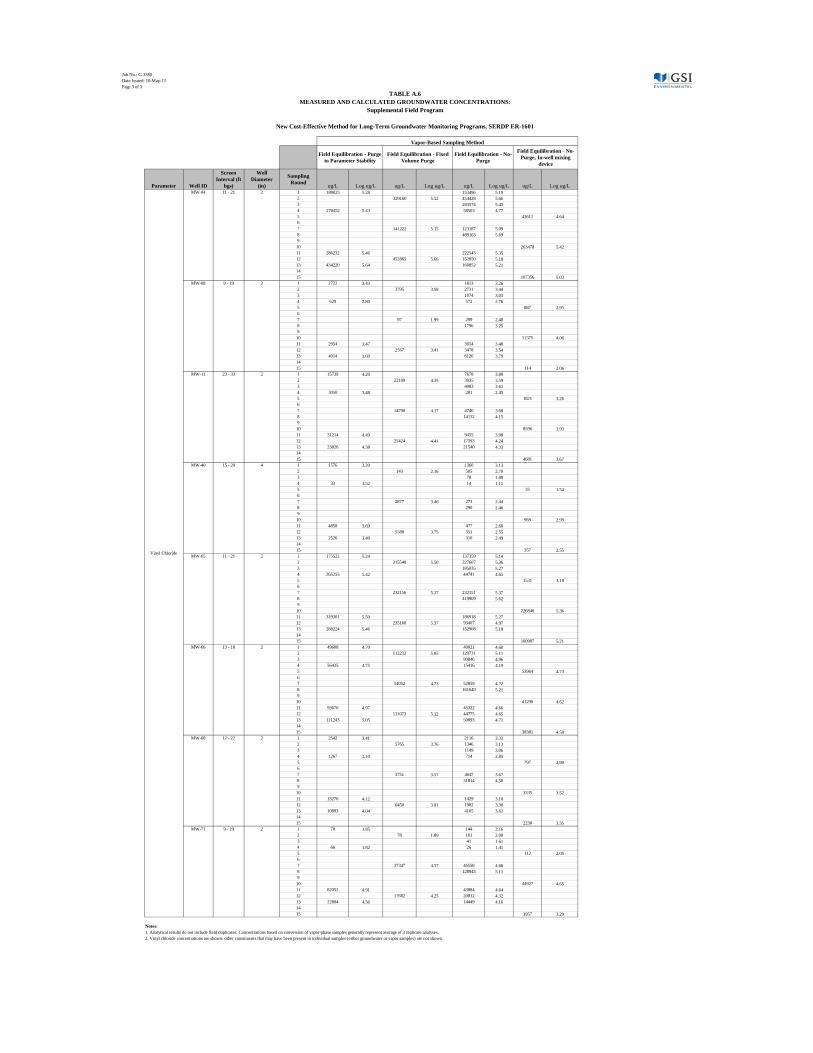
Job No.: G-3380Date Issued: 10-May-13Page 3 of 3
Parameter Well ID
Screen Interval (ft
bgs)
Well Diameter
(in)
Sampling Round ug/L Log ug/L ug/L Log ug/L ug/L Log ug/L ug/L Log ug/L
1 189025 5.28 153496 5.192 329160 5.52 454428 5.663 283574 5.454 270452 5.43 58503 4.775 43611 4.6467 141222 5.15 123187 5.098 489163 5.69910 263478 5.4211 286232 5.46 222543 5.3512 452865 5.66 152850 5.1813 434220 5.64 160852 5.211415 107356 5.031 2722 3.43 1813 3.262 3795 3.58 2731 3.443 1074 3.034 629 2.80 572 2.765 887 2.9567 97 1.99 299 2.488 1796 3.25910 11375 4.0611 2954 3.47 3054 3.4812 2567 3.41 3478 3.5413 4014 3.60 6126 3.791415 114 2.061 15739 4.20 7678 3.892 22189 4.35 3935 3.593 4083 3.614 3050 3.48 281 2.455 1821 3.2667 14790 4.17 4740 3.688 14132 4.15910 8596 3.9311 31214 4.49 9455 3.9812 25424 4.41 17393 4.2413 23826 4.38 21540 4.331415 4681 3.671 1576 3.20 1360 3.132 143 2.16 505 2.703 78 1.894 33 1.52 14 1.155 35 1.5467 2877 3.46 273 2.448 290 2.46910 969 2.9911 4858 3.69 477 2.6812 5588 3.75 351 2.5513 2526 3.40 310 2.491415 357 2.551 175522 5.24 137359 5.142 315548 5.50 227607 5.363 185035 5.274 265255 5.42 44741 4.655 1531 3.1867 232156 5.37 232151 5.378 419909 5.62910 226846 5.3611 319301 5.50 186918 5.2712 235160 5.37 93407 4.9713 288224 5.46 152908 5.181415 160987 5.211 49608 4.70 40021 4.602 112233 5.05 129731 5.113 90846 4.964 56435 4.75 15416 4.195 53964 4.7367 54052 4.73 52859 4.728 161649 5.21910 41290 4.6211 93670 4.97 45322 4.6612 131073 5.12 44775 4.6513 111243 5.05 50893 4.711415 38381 4.581 2542 3.41 2116 3.332 5765 3.76 1346 3.133 1149 3.064 1267 3.10 714 2.855 797 2.9067 3751 3.57 4647 3.678 31814 4.50910 3335 3.5211 13276 4.12 1429 3.1612 6450 3.81 1982 3.3013 10893 4.04 4105 3.611415 2230 3.351 70 1.85 144 2.162 78 1.89 101 2.003 41 1.614 66 1.82 26 1.415 112 2.0567 37347 4.57 45558 4.668 128943 5.11910 44927 4.6511 82052 4.91 43884 4.6412 17682 4.25 20812 4.3213 22804 4.36 14449 4.161415 1957 3.29
Notes:1. Analytical results do not include field duplicates. Concentrations based on conversion of vapor-phase samples generally represent average of 3 replicate analyses.2. Vinyl chloride concentrations are shown; other constituents that may have been present in individual samples (either groundwater or vapor samples) are not shown.
Field Equilibration - Fixed Volume Purge
Field Equilibration - No-Purge
Field Equilibration - No-Purge, In-well mixing
device
Vinyl Chloride
MW-04 11 - 21 2
MW-08 9 - 19 2
MW-11 23 - 33 2
MW-40 15 - 20 4
Field Equilibration - Purge to Parameter Stability
MW-68 12 - 22 2
MW-71 9 - 19 2
MW-65 11 - 21 2
MW-66 13 - 18 2
Vapor-Based Sampling Method
TABLE A.6MEASURED AND CALCULATED GROUNDWATER CONCENTRATIONS:
Supplemental Field Program
New Cost-Effective Method for Long-Term Groundwater Monitoring Programs, SERDP ER-1601
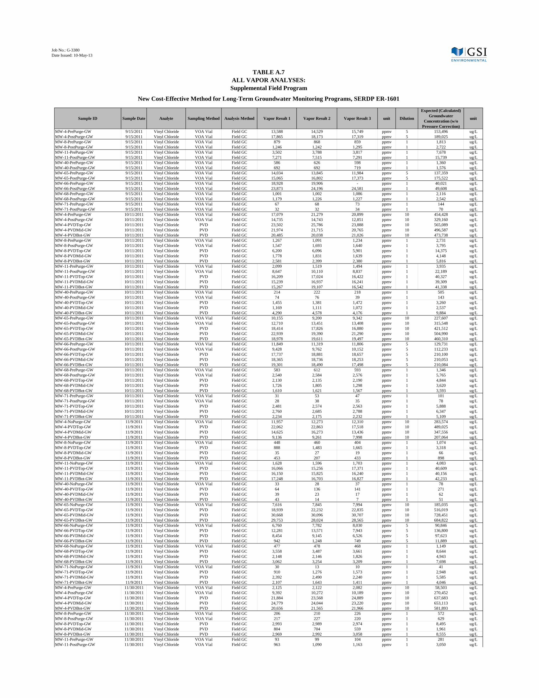
Job No.: G-3380Date Issued: 10-May-13
Sample ID Sample Date Analyte Sampling Method Analysis Method Vapor Result 1 Vapor Result 2 Vapor Result 3 unit Dilution
Expected (Calculated) Groundwater
Concentration (w/o Pressure Correction)
unit
MW-4-PrePurge-GW 9/15/2011 Vinyl Chloride VOA Vial Field GC 13,588 14,529 15,749 ppmv 5 153,496 ug/LMW-4-PostPurge-GW 9/15/2011 Vinyl Chloride VOA Vial Field GC 17,865 18,173 17,319 ppmv 5 189,025 ug/LMW-8-PrePurge-GW 9/15/2011 Vinyl Chloride VOA Vial Field GC 879 868 859 ppmv 1 1,813 ug/LMW-8-PostPurge-GW 9/15/2011 Vinyl Chloride VOA Vial Field GC 1,246 1,242 1,295 ppmv 1 2,722 ug/LMW-11-PrePurge-GW 9/15/2011 Vinyl Chloride VOA Vial Field GC 3,502 3,788 3,817 ppmv 1 7,678 ug/LMW-11-PostPurge-GW 9/15/2011 Vinyl Chloride VOA Vial Field GC 7,271 7,515 7,291 ppmv 1 15,739 ug/LMW-40-PrePurge-GW 9/15/2011 Vinyl Chloride VOA Vial Field GC 586 626 598 ppmv 1 1,360 ug/LMW-40-PostPurge-GW 9/15/2011 Vinyl Chloride VOA Vial Field GC 692 692 719 ppmv 1 1,576 ug/LMW-65-PrePurge-GW 9/15/2011 Vinyl Chloride VOA Vial Field GC 14,034 13,845 11,984 ppmv 5 137,359 ug/LMW-65-PostPurge-GW 9/15/2011 Vinyl Chloride VOA Vial Field GC 15,065 16,802 17,373 ppmv 5 175,522 ug/LMW-66-PrePurge-GW 9/15/2011 Vinyl Chloride VOA Vial Field GC 18,928 19,906 - ppmv 1 40,021 ug/LMW-66-PostPurge-GW 9/15/2011 Vinyl Chloride VOA Vial Field GC 23,873 24,196 24,581 ppmv 1 49,608 ug/LMW-68-PrePurge-GW 9/15/2011 Vinyl Chloride VOA Vial Field GC 1,001 1,002 1,086 ppmv 1 2,116 ug/LMW-68-PostPurge-GW 9/15/2011 Vinyl Chloride VOA Vial Field GC 1,179 1,226 1,227 ppmv 1 2,542 ug/LMW-71-PrePurge-GW 9/15/2011 Vinyl Chloride VOA Vial Field GC 67 68 73 ppmv 1 144 ug/LMW-71-PostPurge-GW 9/15/2011 Vinyl Chloride VOA Vial Field GC 32 32 34 ppmv 1 70 ug/LMW-4-PrePurge-GW 10/11/2011 Vinyl Chloride VOA Vial Field GC 17,079 21,279 20,899 ppmv 10 454,428 ug/LMW-4-PostPurge-GW 10/11/2011 Vinyl Chloride VOA Vial Field GC 14,735 14,743 12,851 ppmv 10 329,160 ug/LMW-4-PVDTop-GW 10/11/2011 Vinyl Chloride PVD Field GC 23,502 25,786 23,888 ppmv 10 565,089 ug/LMW-4-PVDMid-GW 10/11/2011 Vinyl Chloride PVD Field GC 21,974 21,715 20,765 ppmv 10 496,587 ug/LMW-4-PVDBot-GW 10/11/2011 Vinyl Chloride PVD Field GC 20,485 20,038 21,026 ppmv 10 473,738 ug/LMW-8-PrePurge-GW 10/11/2011 Vinyl Chloride VOA Vial Field GC 1,267 1,091 1,234 ppmv 1 2,731 ug/LMW-8-PostPurge-GW 10/11/2011 Vinyl Chloride VOA Vial Field GC 1,547 1,693 1,640 ppmv 1 3,795 ug/LMW-8-PVDTop-GW 10/11/2011 Vinyl Chloride PVD Field GC 6,200 6,096 5,901 ppmv 1 14,375 ug/LMW-8-PVDMid-GW 10/11/2011 Vinyl Chloride PVD Field GC 1,778 1,831 1,639 ppmv 1 4,148 ug/LMW-8-PVDBot-GW 10/11/2011 Vinyl Chloride PVD Field GC 2,581 2,399 2,380 ppmv 1 5,816 ug/LMW-11-PrePurge-GW 10/11/2011 Vinyl Chloride VOA Vial Field GC 2,099 1,519 1,494 ppmv 1 3,935 ug/LMW-11-PostPurge-GW 10/11/2011 Vinyl Chloride VOA Vial Field GC 8,647 10,110 8,837 ppmv 1 22,189 ug/LMW-11-PVDTop-GW 10/11/2011 Vinyl Chloride PVD Field GC 16,209 17,024 16,422 ppmv 1 40,327 ug/LMW-11-PVDMid-GW 10/11/2011 Vinyl Chloride PVD Field GC 15,239 16,937 16,241 ppmv 1 39,309 ug/LMW-11-PVDBot-GW 10/11/2011 Vinyl Chloride PVD Field GC 15,267 19,107 16,542 ppmv 1 41,338 ug/LMW-40-PrePurge-GW 10/11/2011 Vinyl Chloride VOA Vial Field GC 214 222 218 ppmv 1 505 ug/LMW-40-PostPurge-GW 10/11/2011 Vinyl Chloride VOA Vial Field GC 74 76 39 ppmv 1 143 ug/LMW-40-PVDTop-GW 10/11/2011 Vinyl Chloride PVD Field GC 1,455 1,381 1,472 ppmv 1 3,260 ug/LMW-40-PVDMid-GW 10/11/2011 Vinyl Chloride PVD Field GC 1,169 1,111 1,072 ppmv 1 2,537 ug/LMW-40-PVDBot-GW 10/11/2011 Vinyl Chloride PVD Field GC 4,290 4,578 4,176 ppmv 1 9,884 ug/LMW-65-PrePurge-GW 10/11/2011 Vinyl Chloride VOA Vial Field GC 10,155 9,200 9,342 ppmv 10 227,607 ug/LMW-65-PostPurge-GW 10/11/2011 Vinyl Chloride VOA Vial Field GC 12,710 13,451 13,408 ppmv 10 315,548 ug/LMW-65-PVDTop-GW 10/11/2011 Vinyl Chloride PVD Field GC 18,414 17,826 16,880 ppmv 10 421,512 ug/LMW-65-PVDMid-GW 10/11/2011 Vinyl Chloride PVD Field GC 22,939 19,390 21,290 ppmv 10 504,990 ug/LMW-65-PVDBot-GW 10/11/2011 Vinyl Chloride PVD Field GC 18,978 19,611 19,497 ppmv 10 460,310 ug/LMW-66-PrePurge-GW 10/11/2011 Vinyl Chloride VOA Vial Field GC 11,849 11,319 11,806 ppmv 5 129,731 ug/LMW-66-PostPurge-GW 10/11/2011 Vinyl Chloride VOA Vial Field GC 9,428 9,762 10,152 ppmv 5 112,233 ug/LMW-66-PVDTop-GW 10/11/2011 Vinyl Chloride PVD Field GC 17,737 18,881 18,657 ppmv 5 210,100 ug/LMW-66-PVDMid-GW 10/11/2011 Vinyl Chloride PVD Field GC 18,365 18,736 18,253 ppmv 5 210,053 ug/LMW-66-PVDBot-GW 10/11/2011 Vinyl Chloride PVD Field GC 19,301 18,490 17,498 ppmv 5 210,084 ug/LMW-68-PrePurge-GW 10/11/2011 Vinyl Chloride VOA Vial Field GC 583 612 593 ppmv 1 1,346 ug/LMW-68-PostPurge-GW 10/11/2011 Vinyl Chloride VOA Vial Field GC 2,540 2,584 2,576 ppmv 1 5,765 ug/LMW-68-PVDTop-GW 10/11/2011 Vinyl Chloride PVD Field GC 2,130 2,135 2,190 ppmv 1 4,844 ug/LMW-68-PVDMid-GW 10/11/2011 Vinyl Chloride PVD Field GC 1,726 1,805 1,298 ppmv 1 3,620 ug/LMW-68-PVDBot-GW 10/11/2011 Vinyl Chloride PVD Field GC 1,610 1,621 1,567 ppmv 1 3,593 ug/LMW-71-PrePurge-GW 10/11/2011 Vinyl Chloride VOA Vial Field GC 31 53 47 ppmv 1 101 ug/LMW-71-PostPurge-GW 10/11/2011 Vinyl Chloride VOA Vial Field GC 28 38 35 ppmv 1 78 ug/LMW-71-PVDTop-GW 10/11/2011 Vinyl Chloride PVD Field GC 2,481 2,574 2,563 ppmv 1 5,888 ug/LMW-71-PVDMid-GW 10/11/2011 Vinyl Chloride PVD Field GC 2,760 2,685 2,788 ppmv 1 6,347 ug/LMW-71-PVDBot-GW 10/11/2011 Vinyl Chloride PVD Field GC 2,234 2,175 2,232 ppmv 1 5,109 ug/LMW-4-NoPurge-GW 11/9/2011 Vinyl Chloride VOA Vial Field GC 11,957 12,273 12,310 ppmv 10 283,574 ug/LMW-4-PVDTop-GW 11/9/2011 Vinyl Chloride PVD Field GC 22,062 22,863 17,518 ppmv 10 489,025 ug/LMW-4-PVDMid-GW 11/9/2011 Vinyl Chloride PVD Field GC 14,625 16,273 13,436 ppmv 10 347,556 ug/LMW-4-PVDBot-GW 11/9/2011 Vinyl Chloride PVD Field GC 9,136 9,261 7,998 ppmv 10 207,064 ug/LMW-8-NoPurge-GW 11/9/2011 Vinyl Chloride VOA Vial Field GC 448 460 404 ppmv 1 1,074 ug/LMW-8-PVDTop-GW 11/9/2011 Vinyl Chloride PVD Field GC 888 1,483 1,665 ppmv 1 3,318 ug/LMW-8-PVDMid-GW 11/9/2011 Vinyl Chloride PVD Field GC 35 27 19 ppmv 1 66 ug/LMW-8-PVDBot-GW 11/9/2011 Vinyl Chloride PVD Field GC 453 207 433 ppmv 1 898 ug/LMW-11-NoPurge-GW 11/9/2011 Vinyl Chloride VOA Vial Field GC 1,628 1,596 1,703 ppmv 1 4,083 ug/LMW-11-PVDTop-GW 11/9/2011 Vinyl Chloride PVD Field GC 16,066 15,256 17,371 ppmv 1 40,609 ug/LMW-11-PVDMid-GW 11/9/2011 Vinyl Chloride PVD Field GC 16,150 15,825 16,240 ppmv 1 40,156 ug/LMW-11-PVDBot-GW 11/9/2011 Vinyl Chloride PVD Field GC 17,248 16,703 16,827 ppmv 1 42,233 ug/LMW-40-NoPurge-GW 11/9/2011 Vinyl Chloride VOA Vial Field GC 33 28 37 ppmv 1 78 ug/LMW-40-PVDTop-GW 11/9/2011 Vinyl Chloride PVD Field GC 64 136 141 ppmv 1 271 ug/LMW-40-PVDMid-GW 11/9/2011 Vinyl Chloride PVD Field GC 39 23 17 ppmv 1 62 ug/LMW-40-PVDBot-GW 11/9/2011 Vinyl Chloride PVD Field GC 43 14 7 ppmv 1 51 ug/LMW-65-NoPurge-GW 11/9/2011 Vinyl Chloride VOA Vial Field GC 7,616 7,845 7,994 ppmv 10 185,035 ug/LMW-65-PVDTop-GW 11/9/2011 Vinyl Chloride PVD Field GC 18,939 22,232 22,835 ppmv 10 516,019 ug/LMW-65-PVDMid-GW 11/9/2011 Vinyl Chloride PVD Field GC 30,668 30,096 30,707 ppmv 10 728,451 ug/LMW-65-PVDBot-GW 11/9/2011 Vinyl Chloride PVD Field GC 29,753 28,024 28,565 ppmv 10 684,822 ug/LMW-66-NoPurge-GW 11/9/2011 Vinyl Chloride VOA Vial Field GC 6,760 7,782 8,030 ppmv 5 90,846 ug/LMW-66-PVDTop-GW 11/9/2011 Vinyl Chloride PVD Field GC 12,281 13,571 7,943 ppmv 5 136,800 ug/LMW-66-PVDMid-GW 11/9/2011 Vinyl Chloride PVD Field GC 8,454 9,145 6,526 ppmv 5 97,623 ug/LMW-66-PVDBot-GW 11/9/2011 Vinyl Chloride PVD Field GC 942 1,248 749 ppmv 5 11,889 ug/LMW-68-NoPurge-GW 11/9/2011 Vinyl Chloride VOA Vial Field GC 477 478 468 ppmv 1 1,149 ug/LMW-68-PVDTop-GW 11/9/2011 Vinyl Chloride PVD Field GC 3,558 3,487 3,661 ppmv 1 8,644 ug/LMW-68-PVDMid-GW 11/9/2011 Vinyl Chloride PVD Field GC 2,148 2,146 1,826 ppmv 1 4,943 ug/LMW-68-PVDBot-GW 11/9/2011 Vinyl Chloride PVD Field GC 3,062 3,254 3,209 ppmv 1 7,698 ug/LMW-71-NoPurge-GW 11/9/2011 Vinyl Chloride VOA Vial Field GC 30 13 10 ppmv 1 41 ug/LMW-71-PVDTop-GW 11/9/2011 Vinyl Chloride PVD Field GC 910 1,276 1,573 ppmv 1 2,948 ug/LMW-71-PVDMid-GW 11/9/2011 Vinyl Chloride PVD Field GC 2,392 2,490 2,240 ppmv 1 5,585 ug/LMW-71-PVDBot-GW 11/9/2011 Vinyl Chloride PVD Field GC 2,107 1,643 1,411 ppmv 1 4,046 ug/LMW-4-PrePurge-GW 11/30/2011 Vinyl Chloride VOA Vial Field GC 2,125 2,122 2,082 ppmv 10 58,503 ug/LMW-4-PostPurge-GW 11/30/2011 Vinyl Chloride VOA Vial Field GC 9,392 10,272 10,189 ppmv 10 270,452 ug/LMW-4-PVDTop-GW 11/30/2011 Vinyl Chloride PVD Field GC 21,884 23,568 24,889 ppmv 10 637,683 ug/LMW-4-PVDMid-GW 11/30/2011 Vinyl Chloride PVD Field GC 24,779 24,044 23,220 ppmv 10 653,113 ug/LMW-4-PVDBot-GW 11/30/2011 Vinyl Chloride PVD Field GC 20,656 21,565 21,966 ppmv 10 581,893 ug/LMW-8-PrePurge-GW 11/30/2011 Vinyl Chloride VOA Vial Field GC 206 210 226 ppmv 1 572 ug/LMW-8-PostPurge-GW 11/30/2011 Vinyl Chloride VOA Vial Field GC 217 227 220 ppmv 1 629 ug/LMW-8-PVDTop-GW 11/30/2011 Vinyl Chloride PVD Field GC 2,993 2,989 2,974 ppmv 1 8,495 ug/LMW-8-PVDMid-GW 11/30/2011 Vinyl Chloride PVD Field GC 804 704 559 ppmv 1 1,961 ug/LMW-8-PVDBot-GW 11/30/2011 Vinyl Chloride PVD Field GC 2,969 2,992 3,058 ppmv 1 8,555 ug/LMW-11-PrePurge-GW 11/30/2011 Vinyl Chloride VOA Vial Field GC 93 99 104 ppmv 1 281 ug/LMW-11-PostPurge-GW 11/30/2011 Vinyl Chloride VOA Vial Field GC 963 1,090 1,163 ppmv 1 3,050 ug/L
TABLE A.7ALL VAPOR ANALYSES:Supplemental Field Program
New Cost-Effective Method for Long-Term Groundwater Monitoring Programs, SERDP ER-1601

Job No.: G-3380Date Issued: 10-May-13
Sample ID Sample Date Analyte Sampling Method Analysis Method Vapor Result 1 Vapor Result 2 Vapor Result 3 unit Dilution
Expected (Calculated) Groundwater
Concentration (w/o Pressure Correction)
unit
TABLE A.7ALL VAPOR ANALYSES:Supplemental Field Program
New Cost-Effective Method for Long-Term Groundwater Monitoring Programs, SERDP ER-1601
MW-11-PVDTop-GW 11/30/2011 Vinyl Chloride PVD Field GC 8,747 9,384 9,461 ppmv 1 26,104 ug/LMW-11-PVDMid-GW 11/30/2011 Vinyl Chloride PVD Field GC 6,305 6,529 6,532 ppmv 1 18,321 ug/LMW-11-PVDBot-GW 11/30/2011 Vinyl Chloride PVD Field GC 3,229 3,156 2,932 ppmv 1 8,814 ug/LMW-40-PrePurge-GW 11/30/2011 Vinyl Chloride VOA Vial Field GC 5 4 5 ppmv 1 14 ug/LMW-40-PostPurge-GW 11/30/2011 Vinyl Chloride VOA Vial Field GC 13 11 12 ppmv 1 33 ug/LMW-40-PVDTop-GW 11/30/2011 Vinyl Chloride PVD Field GC 92 91 98 ppmv 1 261 ug/LMW-40-PVDMid-GW 11/30/2011 Vinyl Chloride PVD Field GC 106 114 110 ppmv 1 306 ug/LMW-40-PVDBot-GW 11/30/2011 Vinyl Chloride PVD Field GC 57 55 56 ppmv 1 156 ug/LMW-65-PrePurge-GW 11/30/2011 Vinyl Chloride VOA Vial Field GC 1,507 1,582 1,602 ppmv 10 44,741 ug/LMW-65-PostPurge-GW 11/30/2011 Vinyl Chloride VOA Vial Field GC 9,302 9,566 9,540 ppmv 10 265,255 ug/LMW-65-PVDTop-GW 11/30/2011 Vinyl Chloride PVD Field GC 21,230 25,852 21,551 ppmv 10 641,934 ug/LMW-65-PVDMid-GW 11/30/2011 Vinyl Chloride PVD Field GC 17,056 17,975 14,392 ppmv 10 462,260 ug/LMW-65-PVDBot-GW 11/30/2011 Vinyl Chloride PVD Field GC 19,468 18,305 19,416 ppmv 10 534,897 ug/LMW-66-PrePurge-GW 11/30/2011 Vinyl Chloride VOA Vial Field GC 1,017 1,117 1,184 ppmv 5 15,416 ug/LMW-66-PostPurge-GW 11/30/2011 Vinyl Chloride VOA Vial Field GC 3,789 3,939 4,379 ppmv 5 56,435 ug/LMW-66-PVDTop-GW 11/30/2011 Vinyl Chloride PVD Field GC 15,899 17,213 15,971 ppmv 5 228,407 ug/LMW-66-PVDMid-GW 11/30/2011 Vinyl Chloride PVD Field GC 18,210 20,561 20,170 ppmv 5 274,281 ug/LMW-66-PVDBot-GW 11/30/2011 Vinyl Chloride PVD Field GC 17,370 18,264 17,407 ppmv 5 246,825 ug/LMW-68-PrePurge-GW 11/30/2011 Vinyl Chloride VOA Vial Field GC 225 247 262 ppmv 1 714 ug/LMW-68-PostPurge-GW 11/30/2011 Vinyl Chloride VOA Vial Field GC 425 453 477 ppmv 1 1,267 ug/LMW-68-PVDTop-GW 11/30/2011 Vinyl Chloride PVD Field GC 3,637 3,956 3,847 ppmv 1 10,640 ug/LMW-68-PVDMid-GW 11/30/2011 Vinyl Chloride PVD Field GC 4,179 4,101 4,011 ppmv 1 11,431 ug/LMW-68-PVDBot-GW 11/30/2011 Vinyl Chloride PVD Field GC 3,485 3,630 4,044 ppmv 1 10,378 ug/LMW-71-PrePurge-GW 11/30/2011 Vinyl Chloride VOA Vial Field GC 8 9 10 ppmv 1 26 ug/LMW-71-PostPurge-GW 11/30/2011 Vinyl Chloride VOA Vial Field GC 22 23 24 ppmv 1 66 ug/LMW-71-PVDTop-GW 11/30/2011 Vinyl Chloride PVD Field GC 1,757 1,764 1,723 ppmv 1 4,974 ug/LMW-71-PVDMid-GW 11/30/2011 Vinyl Chloride PVD Field GC 142 139 137 ppmv 1 396 ug/LMW-71-PVDBot-GW 11/30/2011 Vinyl Chloride PVD Field GC 2,061 2,203 2,118 ppmv 1 6,053 ug/LMW-4-PostMix-GW 12/20/2011 Vinyl Chloride VOA Vial Field GC 1,268 2,003 1,799 ppmv 10 43,611 ug/LMW-8-PostMix-GW 12/20/2011 Vinyl Chloride VOA Vial Field GC 323 405 321 ppmv 1 887 ug/LMW-11-PostMix-GW 12/20/2011 Vinyl Chloride VOA Vial Field GC 740 616 798 ppmv 1 1,821 ug/LMW-40-PostMix-GW 12/20/2011 Vinyl Chloride VOA Vial Field GC 34 5 4 ppmv 1 35 ug/LMW-65-PostMix-GW 12/20/2011 Vinyl Chloride VOA Vial Field GC 124 91 130 ppmv 5 1,531 ug/LMW-66-PostMix-GW 12/20/2011 Vinyl Chloride VOA Vial Field GC 5,375 2,818 4,380 ppmv 5 53,964 ug/LMW-68-PostMix-GW 12/20/2011 Vinyl Chloride VOA Vial Field GC 395 230 317 ppmv 1 797 ug/LMW-71-PostMix-GW 12/20/2011 Vinyl Chloride VOA Vial Field GC 75 29 25 ppmv 1 112 ug/LMW-4-PVDTop-GW 1/18/2012 Vinyl Chloride PVD Field GC 21,504 20,085 21,352 ppmv 10 581,208 ug/LMW-4-PVDMid-GW 1/18/2012 Vinyl Chloride PVD Field GC 25,091 26,671 24,377 ppmv 10 703,316 ug/LMW-4-PVDBot-GW 1/18/2012 Vinyl Chloride PVD Field GC 7,803 7,136 7,868 ppmv 10 210,463 ug/LMW-8-PVDTop-GW 1/18/2012 Vinyl Chloride PVD Field GC 827 1,082 1,121 ppmv 1 2,712 ug/LMW-8-PVDMid-GW 1/18/2012 Vinyl Chloride PVD Field GC 442 537 384 ppmv 1 1,220 ug/LMW-8-PVDBot-GW 1/18/2012 Vinyl Chloride PVD Field GC 1,655 1,724 1,350 ppmv 1 4,231 ug/LMW-11-PVDTop-GW 1/18/2012 Vinyl Chloride PVD Field GC 2,870 2,445 2,533 ppmv 1 7,042 ug/LMW-11-PVDMid-GW 1/18/2012 Vinyl Chloride PVD Field GC 5,983 7,184 3,472 ppmv 1 14,931 ug/LMW-11-PVDBot-GW 1/18/2012 Vinyl Chloride PVD Field GC 2,519 3,021 596 ppmv 1 5,506 ug/LMW-40-PVDTop-GW 1/18/2012 Vinyl Chloride PVD Field GC 7 2 4 ppmv 1 12 ug/LMW-40-PVDMid-GW 1/18/2012 Vinyl Chloride PVD Field GC 6 28 0 ppmv 1 31 ug/LMW-40-PVDBot-GW 1/18/2012 Vinyl Chloride PVD Field GC 1 3 1 ppmv 1 4 ug/LMW-65-PVDTop-GW 1/18/2012 Vinyl Chloride PVD Field GC 13,000 12,614 11,942 ppmv 10 348,595 ug/LMW-65-PVDMid-GW 1/18/2012 Vinyl Chloride PVD Field GC 18,795 19,133 16,734 ppmv 10 508,389 ug/LMW-65-PVDBot-GW 1/18/2012 Vinyl Chloride PVD Field GC 21,011 22,035 22,791 ppmv 10 613,348 ug/LMW-66-PVDTop-GW 1/18/2012 Vinyl Chloride PVD Field GC 6,223 2,254 11,177 ppmv 5 91,157 ug/LMW-66-PVDMid-GW 1/18/2012 Vinyl Chloride PVD Field GC 7,871 12,792 13,610 ppmv 5 158,961 ug/LMW-66-PVDBot-GW 1/18/2012 Vinyl Chloride PVD Field GC 15,040 13,766 9,298 ppmv 5 176,729 ug/LMW-68-PVDTop-GW 1/18/2012 Vinyl Chloride PVD Field GC 4,084 5,091 4,817 ppmv 1 12,613 ug/LMW-68-PVDMid-GW 1/18/2012 Vinyl Chloride PVD Field GC 2,882 3,661 3,901 ppmv 1 9,415 ug/LMW-68-PVDBot-GW 1/18/2012 Vinyl Chloride PVD Field GC 3,396 4,149 4,631 ppmv 1 10,976 ug/LMW-71-PVDTop-GW 1/18/2012 Vinyl Chloride PVD Field GC 21,290 22,147 25,250 ppmv 1 67,439 ug/LMW-71-PVDMid-GW 1/18/2012 Vinyl Chloride PVD Field GC 23,145 24,252 26,390 ppmv 1 72,446 ug/LMW-71-PVDBot-GW 1/18/2012 Vinyl Chloride PVD Field GC 23,213 24,508 23,599 ppmv 1 70,024 ug/LMW-4-PrePurge-GW 2/8/2012 Vinyl Chloride VOA Vial Field GC 4,054 3,719 4,935 ppmv 10 123,187 ug/LMW-4-PostPurge-GW 2/8/2012 Vinyl Chloride VOA Vial Field GC 5,270 5,196 4,721 ppmv 10 141,222 ug/LMW-4-PVDTop-GW 2/8/2012 Vinyl Chloride PVD Field GC 13,449 21,717 23,485 ppmv 10 554,888 ug/LMW-4-PVDMid-GW 2/8/2012 Vinyl Chloride PVD Field GC 24,794 22,858 23,729 ppmv 10 674,863 ug/LMW-4-PVDBot-GW 2/8/2012 Vinyl Chloride PVD Field GC 22,419 21,451 22,089 ppmv 10 623,389 ug/LMW-8-PrePurge-GW 2/8/2012 Vinyl Chloride VOA Vial Field GC 94 98 85 ppmv 1 299 ug/LMW-8-PostPurge-GW 2/8/2012 Vinyl Chloride VOA Vial Field GC 29 37 36 ppmv 1 97 ug/LMW-8-PVDTop-GW 2/8/2012 Vinyl Chloride PVD Field GC 245 57 232 ppmv 1 511 ug/LMW-8-PVDMid-GW 2/8/2012 Vinyl Chloride PVD Field GC 166 164 174 ppmv 1 482 ug/LMW-8-PVDBot-GW 2/8/2012 Vinyl Chloride PVD Field GC 1,000 924 792 ppmv 1 2,596 ug/LMW-11-PrePurge-GW 2/8/2012 Vinyl Chloride VOA Vial Field GC 1,635 1,847 1,668 ppmv 1 4,740 ug/LMW-11-PostPurge-GW 2/8/2012 Vinyl Chloride VOA Vial Field GC 4,430 5,411 5,302 ppmv 1 14,790 ug/LMW-11-PVDTop-GW 2/8/2012 Vinyl Chloride PVD Field GC 3,699 3,598 3,472 ppmv 1 10,514 ug/LMW-11-PVDMid-GW 2/8/2012 Vinyl Chloride PVD Field GC 6,800 6,693 8,616 ppmv 1 21,579 ug/LMW-11-PVDBot-GW 2/8/2012 Vinyl Chloride PVD Field GC 10,679 4,925 7,974 ppmv 1 23,028 ug/LMW-40-PrePurge-GW 2/8/2012 Vinyl Chloride VOA Vial Field GC 92 100 101 ppmv 1 273 ug/LMW-40-PostPurge-GW 2/8/2012 Vinyl Chloride VOA Vial Field GC 973 1,074 1,097 ppmv 1 2,877 ug/LMW-40-PVDTop-GW 2/8/2012 Vinyl Chloride PVD Field GC 163 234 282 ppmv 1 621 ug/LMW-40-PVDMid-GW 2/8/2012 Vinyl Chloride PVD Field GC 211 258 269 ppmv 1 675 ug/LMW-40-PVDBot-GW 2/8/2012 Vinyl Chloride PVD Field GC 1,834 1,754 1,723 ppmv 1 4,852 ug/LMW-65-PrePurge-GW 2/8/2012 Vinyl Chloride VOA Vial Field GC 7,461 8,482 8,452 ppmv 10 232,151 ug/LMW-65-PostPurge-GW 2/8/2012 Vinyl Chloride VOA Vial Field GC 8,583 8,205 6,935 ppmv 10 232,156 ug/LMW-65-PVDTop-GW 2/8/2012 Vinyl Chloride PVD Field GC 10,762 18,403 18,710 ppmv 10 477,129 ug/LMW-65-PVDMid-GW 2/8/2012 Vinyl Chloride PVD Field GC 18,523 19,148 18,490 ppmv 10 559,517 ug/LMW-65-PVDBot-GW 2/8/2012 Vinyl Chloride PVD Field GC 22,104 23,393 22,168 ppmv 10 673,441 ug/LMW-66-PrePurge-GW 2/8/2012 Vinyl Chloride VOA Vial Field GC 3,794 4,549 2,545 ppmv 5 52,859 ug/LMW-66-PostPurge-GW 2/8/2012 Vinyl Chloride VOA Vial Field GC 3,758 4,404 3,735 ppmv 5 54,052 ug/LMW-66-PVDTop-GW 2/8/2012 Vinyl Chloride PVD Field GC 16,550 16,315 16,062 ppmv 5 225,089 ug/LMW-66-PVDMid-GW 2/8/2012 Vinyl Chloride PVD Field GC 15,378 14,359 14,418 ppmv 5 201,423 ug/LMW-66-PVDBot-GW 2/8/2012 Vinyl Chloride PVD Field GC 17,006 18,397 14,286 ppmv 5 225,602 ug/LMW-68-PrePurge-GW 2/8/2012 Vinyl Chloride VOA Vial Field GC 1,658 1,674 1,519 ppmv 1 4,647 ug/LMW-68-PostPurge-GW 2/8/2012 Vinyl Chloride VOA Vial Field GC 1,320 1,433 1,233 ppmv 1 3,751 ug/LMW-68-PVDTop-GW 2/8/2012 Vinyl Chloride PVD Field GC 4,635 3,001 3,601 ppmv 1 10,562 ug/LMW-68-PVDMid-GW 2/8/2012 Vinyl Chloride PVD Field GC 775 2,923 2,131 ppmv 1 5,482 ug/LMW-68-PVDBot-GW 2/8/2012 Vinyl Chloride PVD Field GC 1,965 2,230 1,611 ppmv 1 5,457 ug/LMW-71-PrePurge-GW 2/8/2012 Vinyl Chloride VOA Vial Field GC 14,378 15,464 14,439 ppmv 1 45,558 ug/LMW-71-PostPurge-GW 2/8/2012 Vinyl Chloride VOA Vial Field GC 12,801 12,964 12,273 ppmv 1 37,347 ug/LMW-71-PVDTop-GW 2/8/2012 Vinyl Chloride PVD Field GC 12,425 13,465 11,726 ppmv 1 36,970 ug/LMW-71-PVDMid-GW 2/8/2012 Vinyl Chloride PVD Field GC 13,852 13,837 15,385 ppmv 1 42,348 ug/LMW-71-PVDBot-GW 2/8/2012 Vinyl Chloride PVD Field GC 21,889 22,367 24,658 ppmv 1 67,663 ug/L
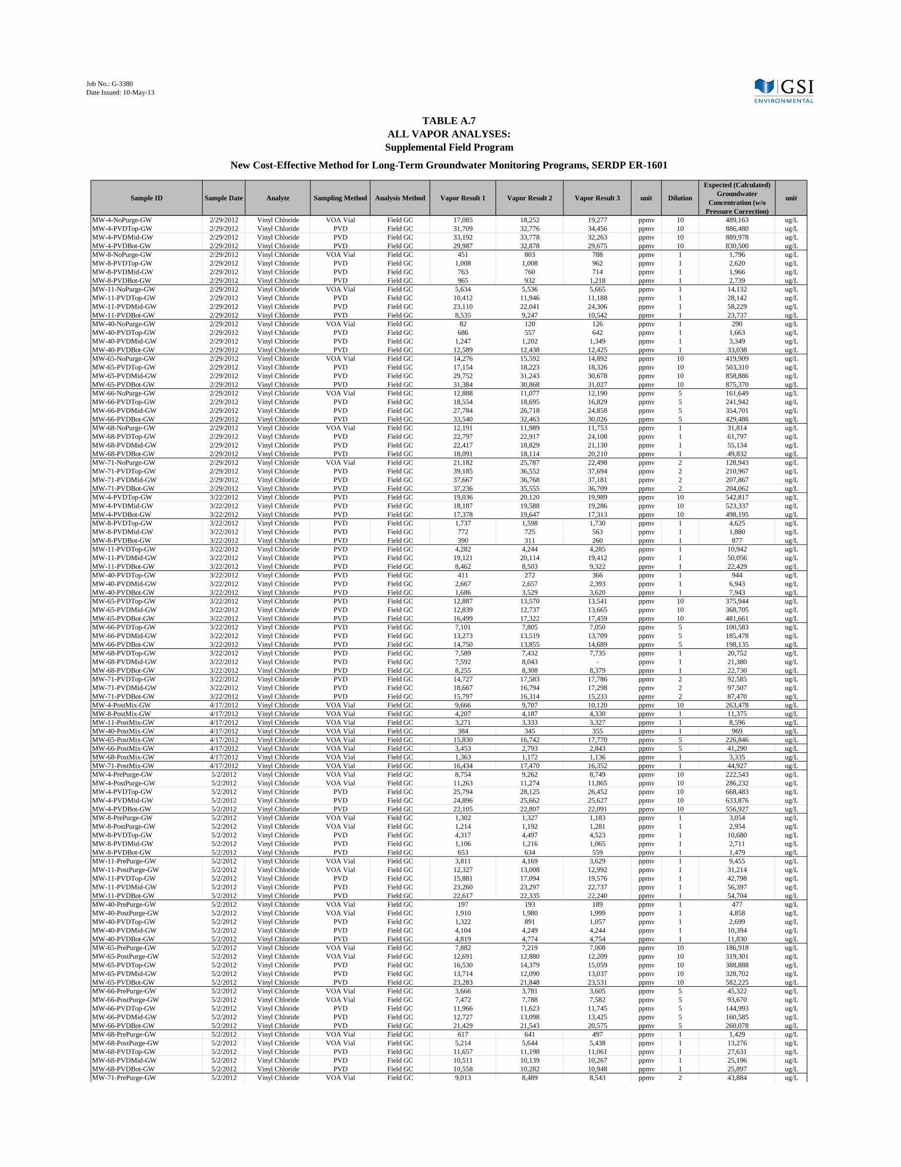
Job No.: G-3380Date Issued: 10-May-13
Sample ID Sample Date Analyte Sampling Method Analysis Method Vapor Result 1 Vapor Result 2 Vapor Result 3 unit Dilution
Expected (Calculated) Groundwater
Concentration (w/o Pressure Correction)
unit
TABLE A.7ALL VAPOR ANALYSES:Supplemental Field Program
New Cost-Effective Method for Long-Term Groundwater Monitoring Programs, SERDP ER-1601
MW-4-NoPurge-GW 2/29/2012 Vinyl Chloride VOA Vial Field GC 17,085 18,252 19,277 ppmv 10 489,163 ug/LMW-4-PVDTop-GW 2/29/2012 Vinyl Chloride PVD Field GC 31,709 32,776 34,456 ppmv 10 886,480 ug/LMW-4-PVDMid-GW 2/29/2012 Vinyl Chloride PVD Field GC 33,192 33,778 32,263 ppmv 10 889,978 ug/LMW-4-PVDBot-GW 2/29/2012 Vinyl Chloride PVD Field GC 29,987 32,878 29,675 ppmv 10 830,500 ug/LMW-8-NoPurge-GW 2/29/2012 Vinyl Chloride VOA Vial Field GC 451 803 788 ppmv 1 1,796 ug/LMW-8-PVDTop-GW 2/29/2012 Vinyl Chloride PVD Field GC 1,008 1,008 962 ppmv 1 2,620 ug/LMW-8-PVDMid-GW 2/29/2012 Vinyl Chloride PVD Field GC 763 760 714 ppmv 1 1,966 ug/LMW-8-PVDBot-GW 2/29/2012 Vinyl Chloride PVD Field GC 965 932 1,218 ppmv 1 2,739 ug/LMW-11-NoPurge-GW 2/29/2012 Vinyl Chloride VOA Vial Field GC 5,634 5,536 5,665 ppmv 1 14,132 ug/LMW-11-PVDTop-GW 2/29/2012 Vinyl Chloride PVD Field GC 10,412 11,946 11,188 ppmv 1 28,142 ug/LMW-11-PVDMid-GW 2/29/2012 Vinyl Chloride PVD Field GC 23,110 22,041 24,306 ppmv 1 58,229 ug/LMW-11-PVDBot-GW 2/29/2012 Vinyl Chloride PVD Field GC 8,535 9,247 10,542 ppmv 1 23,737 ug/LMW-40-NoPurge-GW 2/29/2012 Vinyl Chloride VOA Vial Field GC 82 120 126 ppmv 1 290 ug/LMW-40-PVDTop-GW 2/29/2012 Vinyl Chloride PVD Field GC 686 557 642 ppmv 1 1,663 ug/LMW-40-PVDMid-GW 2/29/2012 Vinyl Chloride PVD Field GC 1,247 1,202 1,349 ppmv 1 3,349 ug/LMW-40-PVDBot-GW 2/29/2012 Vinyl Chloride PVD Field GC 12,589 12,438 12,425 ppmv 1 33,038 ug/LMW-65-NoPurge-GW 2/29/2012 Vinyl Chloride VOA Vial Field GC 14,276 15,592 14,892 ppmv 10 419,909 ug/LMW-65-PVDTop-GW 2/29/2012 Vinyl Chloride PVD Field GC 17,154 18,223 18,326 ppmv 10 503,310 ug/LMW-65-PVDMid-GW 2/29/2012 Vinyl Chloride PVD Field GC 29,752 31,243 30,678 ppmv 10 858,886 ug/LMW-65-PVDBot-GW 2/29/2012 Vinyl Chloride PVD Field GC 31,384 30,868 31,027 ppmv 10 875,370 ug/LMW-66-NoPurge-GW 2/29/2012 Vinyl Chloride VOA Vial Field GC 12,888 11,077 12,190 ppmv 5 161,649 ug/LMW-66-PVDTop-GW 2/29/2012 Vinyl Chloride PVD Field GC 18,554 18,695 16,829 ppmv 5 241,942 ug/LMW-66-PVDMid-GW 2/29/2012 Vinyl Chloride PVD Field GC 27,784 26,718 24,858 ppmv 5 354,701 ug/LMW-66-PVDBot-GW 2/29/2012 Vinyl Chloride PVD Field GC 33,540 32,463 30,026 ppmv 5 429,486 ug/LMW-68-NoPurge-GW 2/29/2012 Vinyl Chloride VOA Vial Field GC 12,191 11,989 11,753 ppmv 1 31,814 ug/LMW-68-PVDTop-GW 2/29/2012 Vinyl Chloride PVD Field GC 22,797 22,917 24,108 ppmv 1 61,797 ug/LMW-68-PVDMid-GW 2/29/2012 Vinyl Chloride PVD Field GC 22,417 18,829 21,130 ppmv 1 55,134 ug/LMW-68-PVDBot-GW 2/29/2012 Vinyl Chloride PVD Field GC 18,091 18,114 20,210 ppmv 1 49,832 ug/LMW-71-NoPurge-GW 2/29/2012 Vinyl Chloride VOA Vial Field GC 21,182 25,787 22,498 ppmv 2 128,943 ug/LMW-71-PVDTop-GW 2/29/2012 Vinyl Chloride PVD Field GC 39,185 36,552 37,694 ppmv 2 210,967 ug/LMW-71-PVDMid-GW 2/29/2012 Vinyl Chloride PVD Field GC 37,667 36,768 37,181 ppmv 2 207,867 ug/LMW-71-PVDBot-GW 2/29/2012 Vinyl Chloride PVD Field GC 37,236 35,555 36,709 ppmv 2 204,062 ug/LMW-4-PVDTop-GW 3/22/2012 Vinyl Chloride PVD Field GC 19,036 20,120 19,989 ppmv 10 542,817 ug/LMW-4-PVDMid-GW 3/22/2012 Vinyl Chloride PVD Field GC 18,187 19,588 19,286 ppmv 10 523,337 ug/LMW-4-PVDBot-GW 3/22/2012 Vinyl Chloride PVD Field GC 17,378 19,647 17,313 ppmv 10 498,195 ug/LMW-8-PVDTop-GW 3/22/2012 Vinyl Chloride PVD Field GC 1,737 1,598 1,730 ppmv 1 4,625 ug/LMW-8-PVDMid-GW 3/22/2012 Vinyl Chloride PVD Field GC 772 725 563 ppmv 1 1,880 ug/LMW-8-PVDBot-GW 3/22/2012 Vinyl Chloride PVD Field GC 390 311 260 ppmv 1 877 ug/LMW-11-PVDTop-GW 3/22/2012 Vinyl Chloride PVD Field GC 4,282 4,244 4,285 ppmv 1 10,942 ug/LMW-11-PVDMid-GW 3/22/2012 Vinyl Chloride PVD Field GC 19,121 20,114 19,412 ppmv 1 50,056 ug/LMW-11-PVDBot-GW 3/22/2012 Vinyl Chloride PVD Field GC 8,462 8,503 9,322 ppmv 1 22,429 ug/LMW-40-PVDTop-GW 3/22/2012 Vinyl Chloride PVD Field GC 411 272 366 ppmv 1 944 ug/LMW-40-PVDMid-GW 3/22/2012 Vinyl Chloride PVD Field GC 2,667 2,657 2,393 ppmv 1 6,943 ug/LMW-40-PVDBot-GW 3/22/2012 Vinyl Chloride PVD Field GC 1,686 3,529 3,620 ppmv 1 7,943 ug/LMW-65-PVDTop-GW 3/22/2012 Vinyl Chloride PVD Field GC 12,887 13,570 13,541 ppmv 10 375,944 ug/LMW-65-PVDMid-GW 3/22/2012 Vinyl Chloride PVD Field GC 12,839 12,737 13,665 ppmv 10 368,705 ug/LMW-65-PVDBot-GW 3/22/2012 Vinyl Chloride PVD Field GC 16,499 17,322 17,459 ppmv 10 481,661 ug/LMW-66-PVDTop-GW 3/22/2012 Vinyl Chloride PVD Field GC 7,101 7,805 7,050 ppmv 5 100,583 ug/LMW-66-PVDMid-GW 3/22/2012 Vinyl Chloride PVD Field GC 13,273 13,519 13,709 ppmv 5 185,478 ug/LMW-66-PVDBot-GW 3/22/2012 Vinyl Chloride PVD Field GC 14,750 13,855 14,689 ppmv 5 198,135 ug/LMW-68-PVDTop-GW 3/22/2012 Vinyl Chloride PVD Field GC 7,589 7,432 7,735 ppmv 1 20,752 ug/LMW-68-PVDMid-GW 3/22/2012 Vinyl Chloride PVD Field GC 7,592 8,043 - ppmv 1 21,380 ug/LMW-68-PVDBot-GW 3/22/2012 Vinyl Chloride PVD Field GC 8,255 8,308 8,379 ppmv 1 22,730 ug/LMW-71-PVDTop-GW 3/22/2012 Vinyl Chloride PVD Field GC 14,727 17,583 17,786 ppmv 2 92,585 ug/LMW-71-PVDMid-GW 3/22/2012 Vinyl Chloride PVD Field GC 18,667 16,794 17,298 ppmv 2 97,507 ug/LMW-71-PVDBot-GW 3/22/2012 Vinyl Chloride PVD Field GC 15,797 16,314 15,233 ppmv 2 87,470 ug/LMW-4-PostMix-GW 4/17/2012 Vinyl Chloride VOA Vial Field GC 9,666 9,707 10,120 ppmv 10 263,478 ug/LMW-8-PostMix-GW 4/17/2012 Vinyl Chloride VOA Vial Field GC 4,207 4,187 4,330 ppmv 1 11,375 ug/LMW-11-PostMix-GW 4/17/2012 Vinyl Chloride VOA Vial Field GC 3,271 3,333 3,327 ppmv 1 8,596 ug/LMW-40-PostMix-GW 4/17/2012 Vinyl Chloride VOA Vial Field GC 384 345 355 ppmv 1 969 ug/LMW-65-PostMix-GW 4/17/2012 Vinyl Chloride VOA Vial Field GC 15,830 16,742 17,770 ppmv 5 226,846 ug/LMW-66-PostMix-GW 4/17/2012 Vinyl Chloride VOA Vial Field GC 3,453 2,793 2,843 ppmv 5 41,290 ug/LMW-68-PostMix-GW 4/17/2012 Vinyl Chloride VOA Vial Field GC 1,363 1,172 1,136 ppmv 1 3,335 ug/LMW-71-PostMix-GW 4/17/2012 Vinyl Chloride VOA Vial Field GC 16,434 17,470 16,352 ppmv 1 44,927 ug/LMW-4-PrePurge-GW 5/2/2012 Vinyl Chloride VOA Vial Field GC 8,754 9,262 8,749 ppmv 10 222,543 ug/LMW-4-PostPurge-GW 5/2/2012 Vinyl Chloride VOA Vial Field GC 11,263 11,274 11,865 ppmv 10 286,232 ug/LMW-4-PVDTop-GW 5/2/2012 Vinyl Chloride PVD Field GC 25,794 28,125 26,452 ppmv 10 668,483 ug/LMW-4-PVDMid-GW 5/2/2012 Vinyl Chloride PVD Field GC 24,896 25,662 25,627 ppmv 10 633,876 ug/LMW-4-PVDBot-GW 5/2/2012 Vinyl Chloride PVD Field GC 22,105 22,807 22,091 ppmv 10 556,927 ug/LMW-8-PrePurge-GW 5/2/2012 Vinyl Chloride VOA Vial Field GC 1,302 1,327 1,183 ppmv 1 3,054 ug/LMW-8-PostPurge-GW 5/2/2012 Vinyl Chloride VOA Vial Field GC 1,214 1,192 1,281 ppmv 1 2,954 ug/LMW-8-PVDTop-GW 5/2/2012 Vinyl Chloride PVD Field GC 4,317 4,497 4,523 ppmv 1 10,680 ug/LMW-8-PVDMid-GW 5/2/2012 Vinyl Chloride PVD Field GC 1,106 1,216 1,065 ppmv 1 2,711 ug/LMW-8-PVDBot-GW 5/2/2012 Vinyl Chloride PVD Field GC 653 634 559 ppmv 1 1,479 ug/LMW-11-PrePurge-GW 5/2/2012 Vinyl Chloride VOA Vial Field GC 3,811 4,169 3,629 ppmv 1 9,455 ug/LMW-11-PostPurge-GW 5/2/2012 Vinyl Chloride VOA Vial Field GC 12,327 13,008 12,992 ppmv 1 31,214 ug/LMW-11-PVDTop-GW 5/2/2012 Vinyl Chloride PVD Field GC 15,881 17,094 19,576 ppmv 1 42,798 ug/LMW-11-PVDMid-GW 5/2/2012 Vinyl Chloride PVD Field GC 23,260 23,297 22,737 ppmv 1 56,397 ug/LMW-11-PVDBot-GW 5/2/2012 Vinyl Chloride PVD Field GC 22,617 22,335 22,240 ppmv 1 54,704 ug/LMW-40-PrePurge-GW 5/2/2012 Vinyl Chloride VOA Vial Field GC 197 193 189 ppmv 1 477 ug/LMW-40-PostPurge-GW 5/2/2012 Vinyl Chloride VOA Vial Field GC 1,910 1,980 1,999 ppmv 1 4,858 ug/LMW-40-PVDTop-GW 5/2/2012 Vinyl Chloride PVD Field GC 1,322 891 1,057 ppmv 1 2,699 ug/LMW-40-PVDMid-GW 5/2/2012 Vinyl Chloride PVD Field GC 4,104 4,249 4,244 ppmv 1 10,394 ug/LMW-40-PVDBot-GW 5/2/2012 Vinyl Chloride PVD Field GC 4,819 4,774 4,754 ppmv 1 11,830 ug/LMW-65-PrePurge-GW 5/2/2012 Vinyl Chloride VOA Vial Field GC 7,882 7,219 7,008 ppmv 10 186,918 ug/LMW-65-PostPurge-GW 5/2/2012 Vinyl Chloride VOA Vial Field GC 12,691 12,880 12,209 ppmv 10 319,301 ug/LMW-65-PVDTop-GW 5/2/2012 Vinyl Chloride PVD Field GC 16,530 14,379 15,059 ppmv 10 388,888 ug/LMW-65-PVDMid-GW 5/2/2012 Vinyl Chloride PVD Field GC 13,714 12,090 13,037 ppmv 10 328,702 ug/LMW-65-PVDBot-GW 5/2/2012 Vinyl Chloride PVD Field GC 23,283 21,848 23,531 ppmv 10 582,225 ug/LMW-66-PrePurge-GW 5/2/2012 Vinyl Chloride VOA Vial Field GC 3,666 3,781 3,605 ppmv 5 45,322 ug/LMW-66-PostPurge-GW 5/2/2012 Vinyl Chloride VOA Vial Field GC 7,472 7,788 7,582 ppmv 5 93,670 ug/LMW-66-PVDTop-GW 5/2/2012 Vinyl Chloride PVD Field GC 11,966 11,623 11,745 ppmv 5 144,993 ug/LMW-66-PVDMid-GW 5/2/2012 Vinyl Chloride PVD Field GC 12,727 13,098 13,425 ppmv 5 160,585 ug/LMW-66-PVDBot-GW 5/2/2012 Vinyl Chloride PVD Field GC 21,429 21,543 20,575 ppmv 5 260,078 ug/LMW-68-PrePurge-GW 5/2/2012 Vinyl Chloride VOA Vial Field GC 617 641 497 ppmv 1 1,429 ug/LMW-68-PostPurge-GW 5/2/2012 Vinyl Chloride VOA Vial Field GC 5,214 5,644 5,438 ppmv 1 13,276 ug/LMW-68-PVDTop-GW 5/2/2012 Vinyl Chloride PVD Field GC 11,657 11,198 11,061 ppmv 1 27,631 ug/LMW-68-PVDMid-GW 5/2/2012 Vinyl Chloride PVD Field GC 10,511 10,139 10,267 ppmv 1 25,196 ug/LMW-68-PVDBot-GW 5/2/2012 Vinyl Chloride PVD Field GC 10,558 10,282 10,948 ppmv 1 25,897 ug/LMW-71-PrePurge-GW 5/2/2012 Vinyl Chloride VOA Vial Field GC 9,013 8,489 8,543 ppmv 2 43,884 ug/L
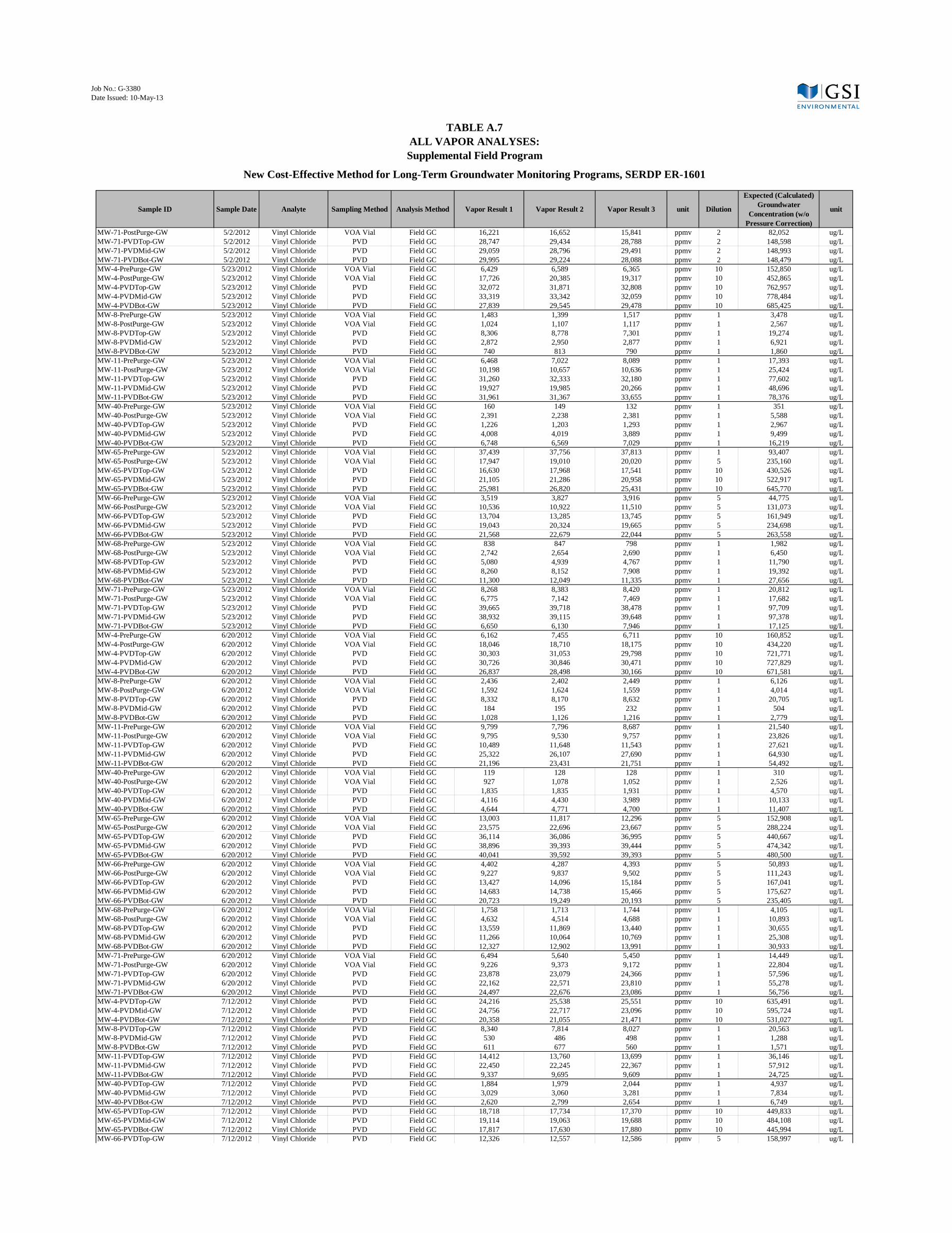
Job No.: G-3380Date Issued: 10-May-13
Sample ID Sample Date Analyte Sampling Method Analysis Method Vapor Result 1 Vapor Result 2 Vapor Result 3 unit Dilution
Expected (Calculated) Groundwater
Concentration (w/o Pressure Correction)
unit
TABLE A.7ALL VAPOR ANALYSES:Supplemental Field Program
New Cost-Effective Method for Long-Term Groundwater Monitoring Programs, SERDP ER-1601
MW-71-PostPurge-GW 5/2/2012 Vinyl Chloride VOA Vial Field GC 16,221 16,652 15,841 ppmv 2 82,052 ug/LMW-71-PVDTop-GW 5/2/2012 Vinyl Chloride PVD Field GC 28,747 29,434 28,788 ppmv 2 148,598 ug/LMW-71-PVDMid-GW 5/2/2012 Vinyl Chloride PVD Field GC 29,059 28,796 29,491 ppmv 2 148,993 ug/LMW-71-PVDBot-GW 5/2/2012 Vinyl Chloride PVD Field GC 29,995 29,224 28,088 ppmv 2 148,479 ug/LMW-4-PrePurge-GW 5/23/2012 Vinyl Chloride VOA Vial Field GC 6,429 6,589 6,365 ppmv 10 152,850 ug/LMW-4-PostPurge-GW 5/23/2012 Vinyl Chloride VOA Vial Field GC 17,726 20,385 19,317 ppmv 10 452,865 ug/LMW-4-PVDTop-GW 5/23/2012 Vinyl Chloride PVD Field GC 32,072 31,871 32,808 ppmv 10 762,957 ug/LMW-4-PVDMid-GW 5/23/2012 Vinyl Chloride PVD Field GC 33,319 33,342 32,059 ppmv 10 778,484 ug/LMW-4-PVDBot-GW 5/23/2012 Vinyl Chloride PVD Field GC 27,839 29,545 29,478 ppmv 10 685,425 ug/LMW-8-PrePurge-GW 5/23/2012 Vinyl Chloride VOA Vial Field GC 1,483 1,399 1,517 ppmv 1 3,478 ug/LMW-8-PostPurge-GW 5/23/2012 Vinyl Chloride VOA Vial Field GC 1,024 1,107 1,117 ppmv 1 2,567 ug/LMW-8-PVDTop-GW 5/23/2012 Vinyl Chloride PVD Field GC 8,306 8,778 7,301 ppmv 1 19,274 ug/LMW-8-PVDMid-GW 5/23/2012 Vinyl Chloride PVD Field GC 2,872 2,950 2,877 ppmv 1 6,921 ug/LMW-8-PVDBot-GW 5/23/2012 Vinyl Chloride PVD Field GC 740 813 790 ppmv 1 1,860 ug/LMW-11-PrePurge-GW 5/23/2012 Vinyl Chloride VOA Vial Field GC 6,468 7,022 8,089 ppmv 1 17,393 ug/LMW-11-PostPurge-GW 5/23/2012 Vinyl Chloride VOA Vial Field GC 10,198 10,657 10,636 ppmv 1 25,424 ug/LMW-11-PVDTop-GW 5/23/2012 Vinyl Chloride PVD Field GC 31,260 32,333 32,180 ppmv 1 77,602 ug/LMW-11-PVDMid-GW 5/23/2012 Vinyl Chloride PVD Field GC 19,927 19,985 20,266 ppmv 1 48,696 ug/LMW-11-PVDBot-GW 5/23/2012 Vinyl Chloride PVD Field GC 31,961 31,367 33,655 ppmv 1 78,376 ug/LMW-40-PrePurge-GW 5/23/2012 Vinyl Chloride VOA Vial Field GC 160 149 132 ppmv 1 351 ug/LMW-40-PostPurge-GW 5/23/2012 Vinyl Chloride VOA Vial Field GC 2,391 2,238 2,381 ppmv 1 5,588 ug/LMW-40-PVDTop-GW 5/23/2012 Vinyl Chloride PVD Field GC 1,226 1,203 1,293 ppmv 1 2,967 ug/LMW-40-PVDMid-GW 5/23/2012 Vinyl Chloride PVD Field GC 4,008 4,019 3,889 ppmv 1 9,499 ug/LMW-40-PVDBot-GW 5/23/2012 Vinyl Chloride PVD Field GC 6,748 6,569 7,029 ppmv 1 16,219 ug/LMW-65-PrePurge-GW 5/23/2012 Vinyl Chloride VOA Vial Field GC 37,439 37,756 37,813 ppmv 1 93,407 ug/LMW-65-PostPurge-GW 5/23/2012 Vinyl Chloride VOA Vial Field GC 17,947 19,010 20,020 ppmv 5 235,160 ug/LMW-65-PVDTop-GW 5/23/2012 Vinyl Chloride PVD Field GC 16,630 17,968 17,541 ppmv 10 430,526 ug/LMW-65-PVDMid-GW 5/23/2012 Vinyl Chloride PVD Field GC 21,105 21,286 20,958 ppmv 10 522,917 ug/LMW-65-PVDBot-GW 5/23/2012 Vinyl Chloride PVD Field GC 25,981 26,820 25,431 ppmv 10 645,770 ug/LMW-66-PrePurge-GW 5/23/2012 Vinyl Chloride VOA Vial Field GC 3,519 3,827 3,916 ppmv 5 44,775 ug/LMW-66-PostPurge-GW 5/23/2012 Vinyl Chloride VOA Vial Field GC 10,536 10,922 11,510 ppmv 5 131,073 ug/LMW-66-PVDTop-GW 5/23/2012 Vinyl Chloride PVD Field GC 13,704 13,285 13,745 ppmv 5 161,949 ug/LMW-66-PVDMid-GW 5/23/2012 Vinyl Chloride PVD Field GC 19,043 20,324 19,665 ppmv 5 234,698 ug/LMW-66-PVDBot-GW 5/23/2012 Vinyl Chloride PVD Field GC 21,568 22,679 22,044 ppmv 5 263,558 ug/LMW-68-PrePurge-GW 5/23/2012 Vinyl Chloride VOA Vial Field GC 838 847 798 ppmv 1 1,982 ug/LMW-68-PostPurge-GW 5/23/2012 Vinyl Chloride VOA Vial Field GC 2,742 2,654 2,690 ppmv 1 6,450 ug/LMW-68-PVDTop-GW 5/23/2012 Vinyl Chloride PVD Field GC 5,080 4,939 4,767 ppmv 1 11,790 ug/LMW-68-PVDMid-GW 5/23/2012 Vinyl Chloride PVD Field GC 8,260 8,152 7,908 ppmv 1 19,392 ug/LMW-68-PVDBot-GW 5/23/2012 Vinyl Chloride PVD Field GC 11,300 12,049 11,335 ppmv 1 27,656 ug/LMW-71-PrePurge-GW 5/23/2012 Vinyl Chloride VOA Vial Field GC 8,268 8,383 8,420 ppmv 1 20,812 ug/LMW-71-PostPurge-GW 5/23/2012 Vinyl Chloride VOA Vial Field GC 6,775 7,142 7,469 ppmv 1 17,682 ug/LMW-71-PVDTop-GW 5/23/2012 Vinyl Chloride PVD Field GC 39,665 39,718 38,478 ppmv 1 97,709 ug/LMW-71-PVDMid-GW 5/23/2012 Vinyl Chloride PVD Field GC 38,932 39,115 39,648 ppmv 1 97,378 ug/LMW-71-PVDBot-GW 5/23/2012 Vinyl Chloride PVD Field GC 6,650 6,130 7,946 ppmv 1 17,125 ug/LMW-4-PrePurge-GW 6/20/2012 Vinyl Chloride VOA Vial Field GC 6,162 7,455 6,711 ppmv 10 160,852 ug/LMW-4-PostPurge-GW 6/20/2012 Vinyl Chloride VOA Vial Field GC 18,046 18,710 18,175 ppmv 10 434,220 ug/LMW-4-PVDTop-GW 6/20/2012 Vinyl Chloride PVD Field GC 30,303 31,053 29,798 ppmv 10 721,771 ug/LMW-4-PVDMid-GW 6/20/2012 Vinyl Chloride PVD Field GC 30,726 30,846 30,471 ppmv 10 727,829 ug/LMW-4-PVDBot-GW 6/20/2012 Vinyl Chloride PVD Field GC 26,837 28,498 30,166 ppmv 10 671,581 ug/LMW-8-PrePurge-GW 6/20/2012 Vinyl Chloride VOA Vial Field GC 2,436 2,402 2,449 ppmv 1 6,126 ug/LMW-8-PostPurge-GW 6/20/2012 Vinyl Chloride VOA Vial Field GC 1,592 1,624 1,559 ppmv 1 4,014 ug/LMW-8-PVDTop-GW 6/20/2012 Vinyl Chloride PVD Field GC 8,332 8,170 8,632 ppmv 1 20,705 ug/LMW-8-PVDMid-GW 6/20/2012 Vinyl Chloride PVD Field GC 184 195 232 ppmv 1 504 ug/LMW-8-PVDBot-GW 6/20/2012 Vinyl Chloride PVD Field GC 1,028 1,126 1,216 ppmv 1 2,779 ug/LMW-11-PrePurge-GW 6/20/2012 Vinyl Chloride VOA Vial Field GC 9,799 7,796 8,687 ppmv 1 21,540 ug/LMW-11-PostPurge-GW 6/20/2012 Vinyl Chloride VOA Vial Field GC 9,795 9,530 9,757 ppmv 1 23,826 ug/LMW-11-PVDTop-GW 6/20/2012 Vinyl Chloride PVD Field GC 10,489 11,648 11,543 ppmv 1 27,621 ug/LMW-11-PVDMid-GW 6/20/2012 Vinyl Chloride PVD Field GC 25,322 26,107 27,690 ppmv 1 64,930 ug/LMW-11-PVDBot-GW 6/20/2012 Vinyl Chloride PVD Field GC 21,196 23,431 21,751 ppmv 1 54,492 ug/LMW-40-PrePurge-GW 6/20/2012 Vinyl Chloride VOA Vial Field GC 119 128 128 ppmv 1 310 ug/LMW-40-PostPurge-GW 6/20/2012 Vinyl Chloride VOA Vial Field GC 927 1,078 1,052 ppmv 1 2,526 ug/LMW-40-PVDTop-GW 6/20/2012 Vinyl Chloride PVD Field GC 1,835 1,835 1,931 ppmv 1 4,570 ug/LMW-40-PVDMid-GW 6/20/2012 Vinyl Chloride PVD Field GC 4,116 4,430 3,989 ppmv 1 10,133 ug/LMW-40-PVDBot-GW 6/20/2012 Vinyl Chloride PVD Field GC 4,644 4,771 4,700 ppmv 1 11,407 ug/LMW-65-PrePurge-GW 6/20/2012 Vinyl Chloride VOA Vial Field GC 13,003 11,817 12,296 ppmv 5 152,908 ug/LMW-65-PostPurge-GW 6/20/2012 Vinyl Chloride VOA Vial Field GC 23,575 22,696 23,667 ppmv 5 288,224 ug/LMW-65-PVDTop-GW 6/20/2012 Vinyl Chloride PVD Field GC 36,114 36,086 36,995 ppmv 5 440,667 ug/LMW-65-PVDMid-GW 6/20/2012 Vinyl Chloride PVD Field GC 38,896 39,393 39,444 ppmv 5 474,342 ug/LMW-65-PVDBot-GW 6/20/2012 Vinyl Chloride PVD Field GC 40,041 39,592 39,393 ppmv 5 480,500 ug/LMW-66-PrePurge-GW 6/20/2012 Vinyl Chloride VOA Vial Field GC 4,402 4,287 4,393 ppmv 5 50,893 ug/LMW-66-PostPurge-GW 6/20/2012 Vinyl Chloride VOA Vial Field GC 9,227 9,837 9,502 ppmv 5 111,243 ug/LMW-66-PVDTop-GW 6/20/2012 Vinyl Chloride PVD Field GC 13,427 14,096 15,184 ppmv 5 167,041 ug/LMW-66-PVDMid-GW 6/20/2012 Vinyl Chloride PVD Field GC 14,683 14,738 15,466 ppmv 5 175,627 ug/LMW-66-PVDBot-GW 6/20/2012 Vinyl Chloride PVD Field GC 20,723 19,249 20,193 ppmv 5 235,405 ug/LMW-68-PrePurge-GW 6/20/2012 Vinyl Chloride VOA Vial Field GC 1,758 1,713 1,744 ppmv 1 4,105 ug/LMW-68-PostPurge-GW 6/20/2012 Vinyl Chloride VOA Vial Field GC 4,632 4,514 4,688 ppmv 1 10,893 ug/LMW-68-PVDTop-GW 6/20/2012 Vinyl Chloride PVD Field GC 13,559 11,869 13,440 ppmv 1 30,655 ug/LMW-68-PVDMid-GW 6/20/2012 Vinyl Chloride PVD Field GC 11,266 10,064 10,769 ppmv 1 25,308 ug/LMW-68-PVDBot-GW 6/20/2012 Vinyl Chloride PVD Field GC 12,327 12,902 13,991 ppmv 1 30,933 ug/LMW-71-PrePurge-GW 6/20/2012 Vinyl Chloride VOA Vial Field GC 6,494 5,640 5,450 ppmv 1 14,449 ug/LMW-71-PostPurge-GW 6/20/2012 Vinyl Chloride VOA Vial Field GC 9,226 9,373 9,172 ppmv 1 22,804 ug/LMW-71-PVDTop-GW 6/20/2012 Vinyl Chloride PVD Field GC 23,878 23,079 24,366 ppmv 1 57,596 ug/LMW-71-PVDMid-GW 6/20/2012 Vinyl Chloride PVD Field GC 22,162 22,571 23,810 ppmv 1 55,278 ug/LMW-71-PVDBot-GW 6/20/2012 Vinyl Chloride PVD Field GC 24,497 22,676 23,086 ppmv 1 56,756 ug/LMW-4-PVDTop-GW 7/12/2012 Vinyl Chloride PVD Field GC 24,216 25,538 25,551 ppmv 10 635,491 ug/LMW-4-PVDMid-GW 7/12/2012 Vinyl Chloride PVD Field GC 24,756 22,717 23,096 ppmv 10 595,724 ug/LMW-4-PVDBot-GW 7/12/2012 Vinyl Chloride PVD Field GC 20,358 21,055 21,471 ppmv 10 531,027 ug/LMW-8-PVDTop-GW 7/12/2012 Vinyl Chloride PVD Field GC 8,340 7,814 8,027 ppmv 1 20,563 ug/LMW-8-PVDMid-GW 7/12/2012 Vinyl Chloride PVD Field GC 530 486 498 ppmv 1 1,288 ug/LMW-8-PVDBot-GW 7/12/2012 Vinyl Chloride PVD Field GC 611 677 560 ppmv 1 1,571 ug/LMW-11-PVDTop-GW 7/12/2012 Vinyl Chloride PVD Field GC 14,412 13,760 13,699 ppmv 1 36,146 ug/LMW-11-PVDMid-GW 7/12/2012 Vinyl Chloride PVD Field GC 22,450 22,245 22,367 ppmv 1 57,912 ug/LMW-11-PVDBot-GW 7/12/2012 Vinyl Chloride PVD Field GC 9,337 9,695 9,609 ppmv 1 24,725 ug/LMW-40-PVDTop-GW 7/12/2012 Vinyl Chloride PVD Field GC 1,884 1,979 2,044 ppmv 1 4,937 ug/LMW-40-PVDMid-GW 7/12/2012 Vinyl Chloride PVD Field GC 3,029 3,060 3,281 ppmv 1 7,834 ug/LMW-40-PVDBot-GW 7/12/2012 Vinyl Chloride PVD Field GC 2,620 2,799 2,654 ppmv 1 6,749 ug/LMW-65-PVDTop-GW 7/12/2012 Vinyl Chloride PVD Field GC 18,718 17,734 17,370 ppmv 10 449,833 ug/LMW-65-PVDMid-GW 7/12/2012 Vinyl Chloride PVD Field GC 19,114 19,063 19,688 ppmv 10 484,108 ug/LMW-65-PVDBot-GW 7/12/2012 Vinyl Chloride PVD Field GC 17,817 17,630 17,880 ppmv 10 445,994 ug/LMW-66-PVDTop-GW 7/12/2012 Vinyl Chloride PVD Field GC 12,326 12,557 12,586 ppmv 5 158,997 ug/L
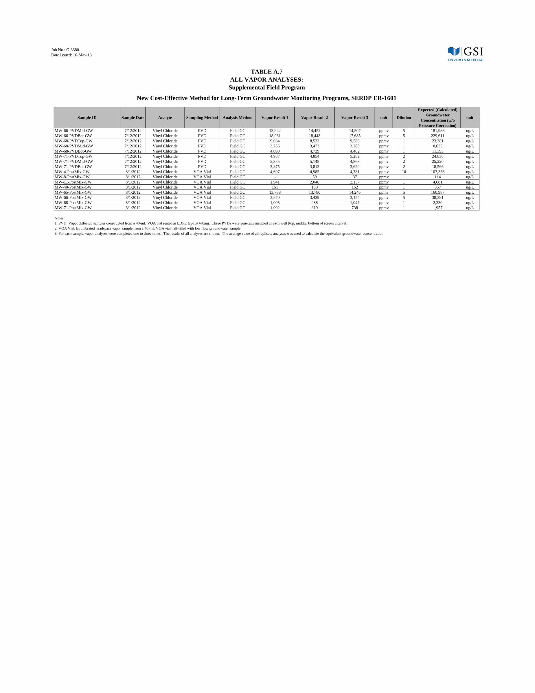
Job No.: G-3380Date Issued: 10-May-13
Sample ID Sample Date Analyte Sampling Method Analysis Method Vapor Result 1 Vapor Result 2 Vapor Result 3 unit Dilution
Expected (Calculated) Groundwater
Concentration (w/o Pressure Correction)
unit
TABLE A.7ALL VAPOR ANALYSES:Supplemental Field Program
New Cost-Effective Method for Long-Term Groundwater Monitoring Programs, SERDP ER-1601
MW-66-PVDMid-GW 7/12/2012 Vinyl Chloride PVD Field GC 13,942 14,452 14,507 ppmv 5 181,986 ug/LMW-66-PVDBot-GW 7/12/2012 Vinyl Chloride PVD Field GC 18,031 18,448 17,685 ppmv 5 229,611 ug/LMW-68-PVDTop-GW 7/12/2012 Vinyl Chloride PVD Field GC 9,034 8,533 9,589 ppmv 1 23,381 ug/LMW-68-PVDMid-GW 7/12/2012 Vinyl Chloride PVD Field GC 3,266 3,473 3,280 ppmv 1 8,635 ug/LMW-68-PVDBot-GW 7/12/2012 Vinyl Chloride PVD Field GC 4,090 4,739 4,402 ppmv 1 11,395 ug/LMW-71-PVDTop-GW 7/12/2012 Vinyl Chloride PVD Field GC 4,987 4,854 5,282 ppmv 2 24,830 ug/LMW-71-PVDMid-GW 7/12/2012 Vinyl Chloride PVD Field GC 5,355 5,148 4,863 ppmv 2 25,220 ug/LMW-71-PVDBot-GW 7/12/2012 Vinyl Chloride PVD Field GC 3,875 3,813 3,620 ppmv 2 18,566 ug/LMW-4-PostMix-GW 8/1/2012 Vinyl Chloride VOA Vial Field GC 4,697 4,985 4,781 ppmv 10 107,356 ug/LMW-8-PostMix-GW 8/1/2012 Vinyl Chloride VOA Vial Field GC - 59 37 ppmv 1 114 ug/LMW-11-PostMix-GW 8/1/2012 Vinyl Chloride VOA Vial Field GC 1,941 2,046 2,137 ppmv 1 4,681 ug/LMW-40-PostMix-GW 8/1/2012 Vinyl Chloride VOA Vial Field GC 151 150 152 ppmv 1 357 ug/LMW-65-PostMix-GW 8/1/2012 Vinyl Chloride VOA Vial Field GC 13,788 13,780 14,246 ppmv 5 160,987 ug/LMW-66-PostMix-GW 8/1/2012 Vinyl Chloride VOA Vial Field GC 3,870 3,439 3,154 ppmv 5 38,381 ug/LMW-68-PostMix-GW 8/1/2012 Vinyl Chloride VOA Vial Field GC 1,005 988 1,047 ppmv 1 2,230 ug/LMW-71-PostMix-GW 8/1/2012 Vinyl Chloride VOA Vial Field GC 1,002 819 738 ppmv 1 1,957 ug/L
Notes:1. PVD: Vapor diffusion sampler constructed from a 40-mL VOA vial sealed in LDPE lay-flat tubing. Three PVDs were generally installed in each well (top, middle, bottom of screen interval).2. VOA Vial: Equilibrated headspace vapor sample from a 40-mL VOA vial half-filled with low flow groundwater sample3. For each sample, vapor analyses were completed one to three times. The results of all analyses are shown. The average value of all replicate analyses was used to calculate the equivalent groundwater concentration.
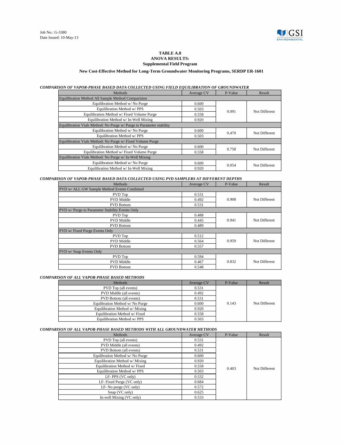
Job No.: G-3380Date Issued: 10-May-13
COMPARISON OF VAPOR-PHASE BASED DATA COLLECTED USING FIELD EQUILIBRATION OF GROUNDWATERMethods Average CV P-Value Result
Equilibration Method w/ No Purge 0.600Equilibration Method w/ PPS 0.503
Equilibration Method w/ Fixed Volume Purge 0.558Equilibration Method w/ In-Well Mixing 0.920
Equilibration Method w/ No Purge 0.600Equilibration Method w/ PPS 0.503
Equilibration Method w/ No Purge 0.600Equilibration Method w/ Fixed Volume Purge 0.558
Equilibration Method w/ No Purge 0.600Equilibration Method w/ In-Well Mixing 0.920
COMPARISON OF VAPOR-PHASE BASED DATA COLLECTED USING PVD SAMPLERS AT DIFFERENT DEPTHSMethods Average CV P-Value Result
PVD Top 0.531PVD Middle 0.492PVD Bottom 0.531
PVD w/ Purge to Parameter Stability Events OnlyPVD Top 0.488
PVD Middle 0.445PVD Bottom 0.489
PVD Top 0.512PVD Middle 0.564PVD Bottom 0.557
PVD Top 0.594PVD Middle 0.467PVD Bottom 0.548
COMPARISON OF ALL VAPOR-PHASE BASED METHODSMethods Average CV P-Value Result
PVD Top (all events) 0.531PVD Middle (all events) 0.492PVD Bottom (all events) 0.531
Equlibration Method w/ No Purge 0.600Equilibration Method w/ Mixing 0.920Equilibration Method w/ Fixed 0.558Equilibration Method w/ PPS 0.503
COMPARISON OF ALL VAPOR-PHASE BASED METHODS WITH ALL GROUNDWATER METHODSMethods Average CV P-Value Result
PVD Top (all events) 0.531PVD Middle (all events) 0.492PVD Bottom (all events) 0.531
Equlibration Method w/ No Purge 0.600Equilibration Method w/ Mixing 0.920Equilibration Method w/ Fixed 0.558Equilibration Method w/ PPS 0.503
LF- PPS (VC only) 0.532LF- Fixed Purge (VC only) 0.684
LF- No purge (VC only) 0.572Snap (VC only) 0.625
In-well Mixing (VC only) 0.533
0.403 Not Different
0.908 Not Different
0.941 Not Different
PVD w/ Fixed Purge Events Only
0.959 Not Different
PVD w/ Snap Events Only
0.832 Not Different
0.143 Not Different
0.091 Not Different
PVD w/ ALL GW Sample Method Events Combined
Equilibration Vials Method: No Purge w/ Purge to Parameter stability
0.470 Not Different
Equilibration Vials Method: No Purge w/ Fixed Volume Purge
0.758 Not Different
Equilibration Vials Method: No Purge w/ In-Well Mixing
0.054 Not Different
TABLE A.8ANOVA RESULTS:
Supplemental Field Program
New Cost-Effective Method for Long-Term Groundwater Monitoring Programs, SERDP ER-1601
Equilibration Method All Sample Method Comparision
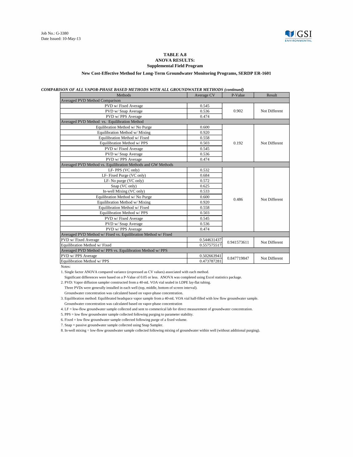
Job No.: G-3380Date Issued: 10-May-13
TABLE A.8ANOVA RESULTS:
Supplemental Field Program
New Cost-Effective Method for Long-Term Groundwater Monitoring Programs, SERDP ER-1601
COMPARISON OF ALL VAPOR-PHASE BASED METHODS WITH ALL GROUNDWATER METHODS (continued)Methods Average CV P-Value Result
PVD w/ Fixed Average 0.545PVD w/ Snap Average 0.536PVD w/ PPS Average 0.474
Equlibration Method w/ No Purge 0.600Equilibration Method w/ Mixing 0.920Equilibration Method w/ Fixed 0.558Equilibration Method w/ PPS 0.503
PVD w/ Fixed Average 0.545PVD w/ Snap Average 0.536PVD w/ PPS Average 0.474
LF- PPS (VC only) 0.532LF- Fixed Purge (VC only) 0.684
LF- No purge (VC only) 0.572Snap (VC only) 0.625
In-well Mixing (VC only) 0.533Equlibration Method w/ No Purge 0.600Equilibration Method w/ Mixing 0.920Equilibration Method w/ Fixed 0.558Equilibration Method w/ PPS 0.503
PVD w/ Fixed Average 0.545PVD w/ Snap Average 0.536PVD w/ PPS Average 0.474
PVD w/ Fixed Average 0.544631437Equilibration Method w/ Fixed 0.557575517
PVD w/ PPS Average 0.502663941Equilibration Method w/ PPS 0.473787281Notes:1. Single factor ANOVA compared variance (expressed as CV values) associated with each method. Significant differences were based on a P-Value of 0.05 or less. ANOVA was completed using Excel statistics package. 2. PVD: Vapor diffusion sampler constructed from a 40-mL VOA vial sealed in LDPE lay-flat tubing. Three PVDs were generally installed in each well (top, middle, bottom of screen interval). Groundwater concentration was calculated based on vapor-phase concentration.3. Equilibration method: Equilibrated headspace vapor sample from a 40-mL VOA vial half-filled with low flow groundwater sample. Groundwater concentration was calculated based on vapor-phase concentration4. LF = low-flow groundwater sample collected and sent to commerical lab for direct measurement of groundwater concentration. 5. PPS = low flow groundwater sample collected following purging to parameter stability.6. Fixed = low flow groundwater sample collected following purge of a fixed volume.7. Snap = passive groundwater sample collected using Snap Sampler.8. In-well mixing = low-flow groundwater sample collected following mixing of groundwater within well (without additional purging).
Averaged PVD Method Comparison
0.902 Not Different
Averaged PVD Method vs. Equilibration Method
0.192 Not Different
Averaged PVD Method w/ PPS vs. Equilibration Method w/ PPS
0.847719847 Not Different
Averaged PVD Method vs. Equilibration Methods and GW Methods
0.486 Not Different
Averaged PVD Method w/ Fixed vs. Equilibration Method w/ Fixed
0.941573611 Not Different

Job No.: G-3380Date Issued: 10-May-13
COMPARISON OF VAPOR-PHASE BASED DATA COLLECTED USING FIELD EQUILIBRATION OF GROUNDWATER
Method 1 Method 2 P-Value Result t-Value Result R Result BiasEquilibration Method w/ Fixed Volume Purge Equilibration Method w/ In-Well Mixing 0.101 Not Different 3.297 Different 2,34 Different Mixing is more variable than FixedEquilibration Method w/ Fixed Volume Purge Equilibration Method w/ Purge to Parameter Stability 0.743 Not Different -0.470 Not Different 17,19 Not Different -Equilibration Method w/ Fixed Volume Purge Equilibration Method w/ No Purge 0.758 Not Different -0.916 Not Different 10,26 Not Different -
Equilibration Method w/ In-Well Mixing Equilibration Method w/ Purge to Parameter Stability 0.058 Not Different* 2.630 Different 3,33 Different Mixing is more Variable than PPSEquilibration Method w/ In-Well Mixing Equilibration Method w/ No Purge 0.054 Not Different* - - - - -
Equilibration Method w/ Purge to Parameter Stability Equilibration Method w/ No Purge 0.47 Not Different -0.205 Not Different 16,20 Not Different -
COMPARISON OF VAPOR-PHASE BASED DATA COLLECTED USING PVD SAMPLERS AT DIFFERENT DEPTHS
Method 1 Method 2 P-Value Result t-Value Result R Result BiasPVD Top w/ Fixed Purge PVD Middle w/ Fixed Purge 0.795 Not Different 0.493 Not Different 18,18 Not Different -PVD Top w/ Fixed Purge PVD Bottom w/ Fixed Purge 0.813 Not Different 0.438 Not Different 17,19 Not Different -
PVD Middle w/ Fixed Purge PVD Bottom w/ Fixed Purge 0.973 Not Different -0.077 Not Different 16,20 Not Different -PVD Top w/ Snap PVD Middle w/ Snap 0.535 Not Different -1.521 Not Different 8,28 Not Different -PVD Top w/ Snap PVD Bottom w/ Snap 0.835 Not Different -0.523 Not Different 14,22 Not Different -
PVD Middle w/ Snap PVD Bottom w/ Snap 0.712 Not Different 0.646 Not Different 10,26 Not Different -PVD Top w/ PPS PVD Middle w/ PPS 0.781 Not Different -1.206 Not Different 10,26 Not Different -PVD Top w/ PPS PVD Bottom w/ PPS 0.997 Not Different 0.008 Not Different 16,20 Not Different -
PVD Middle w/ PPS PVD Bottom w/ PPS 0.755 Not Different 0.607 Not Different 24,12 Not Different -PVD Top w/ Fixed PVD Top w/ Snap 0.675 Not Different 0.851 Not Different 13,23 Not Different -PVD Top w/ Fixed PVD Top w/ PPS 0.886 Not Different -0.316 Not Different 15,21 Not Different - PVD Top w/ Snap PVD Top w/ PPS 0.568 Not Different -1.251 Not Different 12,24 Not Different -
PVD Middle w/ Fixed PVD Middle w/ Snap 0.642 Not Different -0.857 Not Different 14,22 Not Different -PVD Middle w/ Fixed PVD Middle w/ PPS 0.528 Not Different -1.409 Not Different 9,27 Not Different -PVD Middle w/ Snap PVD Middle w/ PPS 0.897 Not Different -0.189 Not Different 17,19 Not Different -PVD Bottom w/ Fixed PVD Bottom w/ Snap 0.965 Not Different -0.078 Not Different 15,21 Not Different -PVD Bottom w/ Fixed PVD Bottom w/ PPS 0.681 Not Different -0.530 Not Different 17,19 Not Different -PVD Bottom w/ Snap PVD Bottom w/ PPS 0.754 Not Different -0.424 Not Different 16,20 Not Different -
COMPARISON OF ALL VAPOR-PHASE BASED METHODS USING AVERAGED PVD DATA
Method 1 Method 2 P-Value Result t-Value Result R Result BiasPVD Avg. w/ PPS Equilibration Method w/ PPS 0.607 Not Different 1.238 Not Different 9,27 No Difference -
PVD Avg. w/ Fixed Equilibration Method w/ Fixed 0.666 Not Different 0.623 Not Different 14,22 No Difference -PVD Avg. w/ Fixed Equilibration Method w/ NP (before fixed) 0.188 Not Different 1.668 Not Different* 8,28 No Difference -PVD Avg. w/ PPS Equilibration Method w/ NP (before PPS) 0.554 Not Different 1.238 Not Different 9,27 No Difference -
Notes:1. Parametric (two-sample and paired t-tests) and non-parametric (Wilcoxson Signed Rank test) methods were used to compare variance (expressed as CV values) associated with each method. Tests were completed using Excel statistics package. 2. PVD: Vapor diffusion sampler constructed from a 40-mL VOA vial sealed in LDPE lay-flat tubing. Three PVDs were generally installed in each well (top, middle, bottom of screen interval). Groundwater concentration was calculated based on vapor-phase concentration.3. Equilibration method: Equilibrated headspace vapor sample from a 40-mL VOA vial half-filled with low flow groundwater sample. Groundwater concentration was calculated based on vapor-phase concentration.4. LF = low-flow groundwater sample collected and sent to commerical lab for direct measurement of groundwater concentration. 5. PPS = low flow groundwater sample collected following purging to parameter stability.6. Fixed = low flow groundwater sample collected following purge of a fixed volume.7. Snap = passive groundwater sample collected using Snap Sampler.8. In-well mixing = low-flow groundwater sample collected following mixing of groundwater within well (without additional purging).9. n=8 for Fixed, Mixing, PPS n=16 for NP
TABLE A.9PARAMETRIC AND NON-PARAMETRIC TWO-SAMPLE TEST RESULTS:
Supplemental Field Program
New Cost-Effective Method for Long-Term Groundwater Monitoring Programs, SERDP ER-1601
Equilibration Method Two Sample T Test Paired T Test Wilcoxon Signed Rank Test
PVD Method Two Sample T Test Paired T Test Wilcoxon Signed Rank Test
PVD Method Two Sample T Test Paired T Test Wilcoxon Signed Rank Test

Job No.: G-3380Date Issued: 10-May-13Page 1 of 1
INPUT PARAMETERS VAPOR-BASED LOW-FLOW VAPOR-BASED PASSIVE DIFFUSION BAG (GW) LOW-FLOWScenarios: 1-4 5-6 7 8 9 Supervising ESGH $155
# of Wells Sampled at each Sampling Event 20 20 20 20 20 ESGH III $130Total number of Sampling Events 15 15 15 15 15 ESGH II $105
Duplicate GW Samples %: - 10 - 10 10 ESGH I $90 # of PVD Samples Per Well: 1 - 3 - - Tech $75
# of Passive Diffusion Bags per Well: - - - 3 -# of GW Samples per Well (Multil-Level MW): - 1 - - 3
Time for each GC analysis (min): 10 - 10 - - *will vary based on VOCs monitored
Max expected GC analysis time (min/8-hrs): 360 - 360 - - *assumes 6-hour continuous analysis
Travel Time to Site (1-way: hrs): 1 1 1 1 1Max # of Wells Instrumented (per 8-hrs): 30 - 30 30 - *installation of PVD sampling assembly ~2 weeks before first sampling event; incorporated at end of subsequent sampling events
Max Number of Wells Sampled (per 8-hrs): - 8 - 29 3 *Calculated below if "-"
Scenarios: 1-4 5-6 7 8 9Sampler Installation Days Required: 15 - 15 15 -
Sampling Days Required: 17 38 50 10 100GC replicate analyses per PVD sampler: 1 - 1 - - *duplicate recommended for routine monitoring
Total GC analysis time per well (min): 20 - 60 - -Max Number of Wells Sampled (per 8-hrs): 18 - 6 - -
GW Dups Collected: - 30 - 90 90 *Assumes dups rounded to nearest sample #; i.e. 0-14 samples = 1 dup, 15-24 samples = 2 dups, 25-34 samples = 3 dups
Purge Water Generated (gals): - 600 - 450 1800 *Assumed 2-gallons per well for Low-Flow and 0.5 gallon for Passive Diffusion Bags
SCENARIO 1 SCENARIO 2 SCENARIO 3 SCENARIO 4 SCENARIO 5 SCENARIO 6 SCENARIO 7 SCENARIO 8 SCENARIO 9Technology type= Vapor-Based Vapor-Based Vapor-Based Vapor-Based Low-Flow GW Low-Flow GW Vapor-Based Passive Diffusion Bag GW Low-Flow GW
Travel option= In Town Out of Town In Town Out of Town In Town Out of Town In Town In Town In TownGC vs. Lab= GC Rental GC Rental GC Purchase GC Purchase Laboratory Laboratory GC Rental Laboratory Laboratory
# of samples per location= 1 1 1 1 1 1 3 3 3COST ELEMENT DATA TRACKEDTASK 1. Preparation and Sample CollectionProject management (Sup. ESGH and ESGH III) $1,140 $1,140 $1,140 $1,140 $1,140 $1,140 $1,140 $1,140 $1,140 LaborSampler Assembly (ESGH III) $6,500 $6,500 $6,500 $6,500 $0 $0 $19,500 $0 $0 Airfare, per diem, etc.Well Assemply Prep (ESGH III) $650 $650 $650 $650 $0 $0 $650 $650 $0 Material costProcure Materials (Tech) $150 $150 $150 $150 $0 $0 $150 $0 $0Installation Mobilization/Demobilization (Tech) $11,250 $11,250 $11,250 $11,250 $0 $0 $11,250 $11,250 $0Sampler Material ($2 per PVD or $20 per PDB) $600 $600 $600 $600 $0 $0 $1,800 $19,800 $0Well Caps $500 $500 $500 $500 $0 $0 $500 $0 $0Weights $500 $500 $500 $500 $0 $0 $500 $0 $0Pump $0 $0 $0 $0 $1,330 $1,330 $0 $0 $3,500Low-flow sampling equipment $0 $0 $0 $0 $3,610 $3,610 $0 $950 $9,500Level D PPE $960 $960 $960 $960 $2,280 $2,280 $1,950 $600 $6,000Purge Water Management $0 $0 $0 $0 $1,100 $1,100 $0 $900 $3,300Field Vehicle $2,400 $2,400 $2,400 $2,400 $2,850 $2,850 $4,875 $750 $7,500Sampler Assembly Installation (Tech) $6,000 $6,000 $6,000 $6,000 $0 $0 $6,000 $0 $0Sampling Mobilization/Demobilization
ESGH III $4,420 $4,420 $4,420 $4,420 $0 $0 $13,000 $0 $0ESGH I $0 $0 $0 $0 $6,840 $6,840 $0 $1,800 $18,000Tech $0 $0 $0 $0 $5,700 $5,700 $0 $1,500 $15,000
On-Site Sample Collection (ESGH III)ESGH III $17,680 $17,680 $17,680 $17,680 $0 $0 $52,000 $0 $0ESGH I $0 $0 $0 $0 $27,360 $27,360 $0 $7,200 $72,000Tech $0 $0 $0 $0 $22,800 $22,800 $0 $6,000 $60,000
Travel (ESGH III) $0 $11,250 $0 $11,250 $0 $22,500 $0 $0 $0Per Diem (ESGH III) $0 $3,415 $0 $3,415 $0 $15,200 $0 $0 $0Waste disposal $100 $100 $100 $100 $1,200 $1,200 $100 $900 $3,600Miscellaneous costs $1,000 $2,000 $1,000 $2,000 $1,000 $2,000 $1,000 $3,000 $5,000Task 1 Total $53,850 $69,515 $53,850 $69,515 $77,210 $115,910 $114,415 $56,440 $204,540
TASK 2. Sample AnalysisProject management $1,140 $1,140 $1,140 $1,140 $1,140 $1,140 $1,140 $1,140 $1,140 LaborGC rental $6,800 $6,800 $0 $0 $0 $0 $20,000 $0 $0 Material costGC Purchase $0 $0 $30,000 $30,000 $0 $0 $0 $0 $0Calibration Gas $1,000 $1,000 $1,000 $1,000 $0 $0 $1,000 $0 $0Carrier Gas $500 $500 $500 $500 $0 $0 $500 $0 $0Analytical $0 $0 $0 $0 $41,375 $41,375 $0 $123,875 $123,875Shipping $0 $6,000 $0 $10,500 $0 $1,655 $0 $1,655 $4,955Miscellaneous costs $2,000 $2,000 $5,000 $5,000 $2,000 $3,000 $2,000 $3,000 $5,000TASK 2 Total $11,440 $17,440 $37,640 $48,140 $44,515 $47,170 $24,640 $129,670 $134,970
TASK 3. Data Management and ReportingProject management $1,140 $1,140 $1,140 $1,140 $1,140 $1,140 $1,140 $1,140 $1,140 LaborData Analysis (ESGH III) $6,500 $6,500 $6,500 $6,500 $6,500 $6,500 $19,500 $19,500 $19,500Data Table/Letter Report (ESGH I, II) $5,340 $5,340 $5,340 $5,340 $5,340 $5,340 $5,340 $14,340 $14,340Miscellaneous costs $1,000 $1,000 $1,000 $1,000 $1,000 $1,000 $1,000 $2,000 $5,000TASK 3 Total $13,980 $13,980 $13,980 $13,980 $13,980 $13,980 $26,980 $36,980 $39,980
CONTINGENCY (15%) $11,891 $15,140 $15,821 $19,745 $20,356 $26,559 $24,905 $33,464 $56,924TOTAL COST $91,161 $116,075 $121,291 $151,380 $156,061 $203,619 $190,940 $256,554 $436,414COST PER WELL LOCATION $304 $387 $404 $505 $520 $679 $636 $855 $1,455COST PER SAMPLE $304 $387 $404 $505 $473 $617 $212 $259 $441
Vapor-based GW sampling using passive vapor diffusion (PVD) samplers:· Scenario 1: in town and GC rental· Scenario 2: out of town and GC rental· Scenario 3: in town and GC purchase· Scenario 4: out of town and GC purchase
Alternative Technology scenarios (conventional low-flow GW sampling):· Scenario 5: in town· Scenario 6: out of town
Multi-level sampling scenarios (all in town):· Scenario 7: 5 samples per location using passive vapor diffusin (PVD) samplers (vapor)· Scenario 8: 5 samples per location using passive diffusion bag (PDB) samplers (groundwater)· Scenario 9: 5 samples per location using low-flow groundwater from multi-level monitoring well network
CALCULATED PARAMETERS
TABLE A.10COST MODEL AND RESULTS:
New Cost-Effective Method for Long-Term Groundwater Monitoring Programs, SERDP ER-1601
Labor Hourly Rates
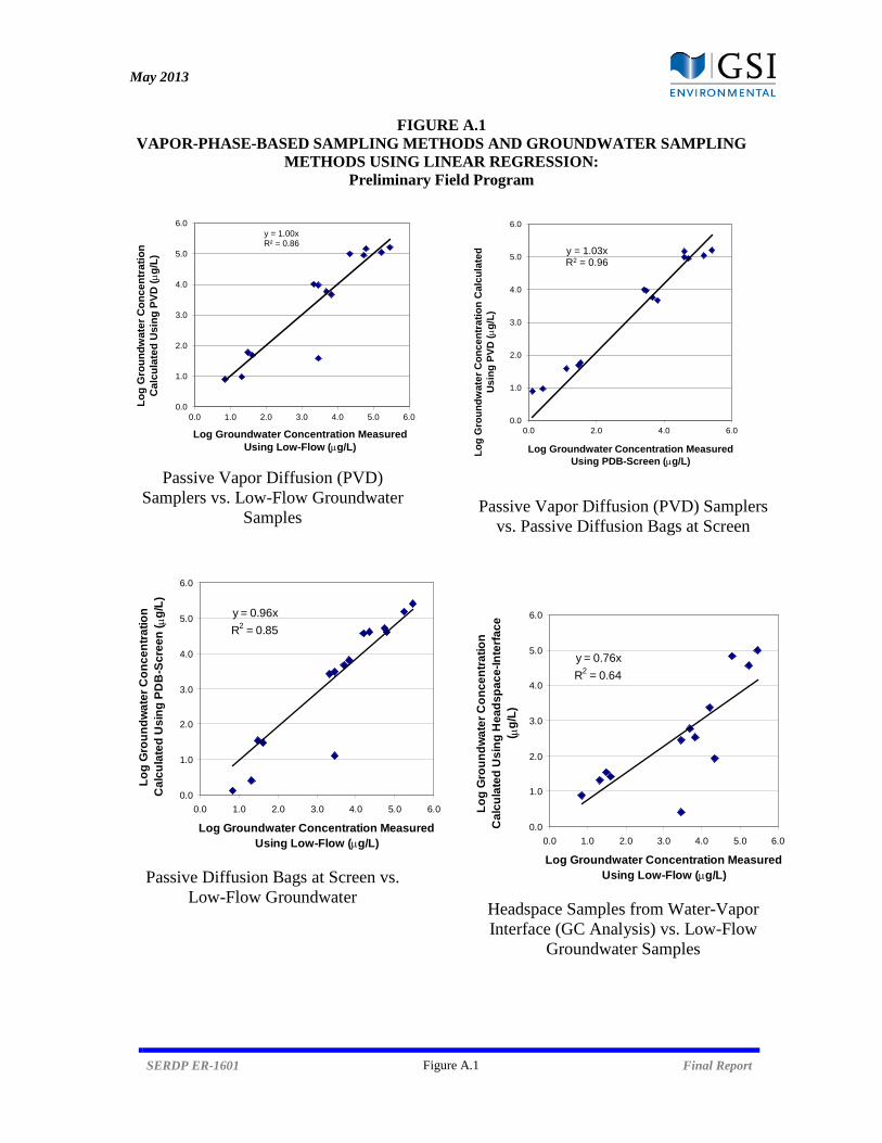
May 2013
FIGURE A.1 VAPOR-PHASE-BASED SAMPLING METHODS AND GROUNDWATER SAMPLING
METHODS USING LINEAR REGRESSION: Preliminary Field Program
SERDP ER-1601 Figure A.1 Final Report
Passive Vapor Diffusion (PVD)
Samplers vs. Low-Flow Groundwater Samples
Passive Diffusion Bags at Screen vs.
Low-Flow Groundwater
Passive Vapor Diffusion (PVD) Samplers vs. Passive Diffusion Bags at Screen
Headspace Samples from Water-Vapor Interface (GC Analysis) vs. Low-Flow
Groundwater Samples
y = 1.00xR² = 0.86
0.0
1.0
2.0
3.0
4.0
5.0
6.0
0.0 1.0 2.0 3.0 4.0 5.0 6.0
Lo
g G
rou
nd
wa
ter
Co
nc
en
tra
tio
n
Ca
lcu
late
d U
sin
g P
VD
(µg
/L)
Log Groundwater Concentration Measured Using Low-Flow (µg/L)
y = 0.96xR2 = 0.85
0.0
1.0
2.0
3.0
4.0
5.0
6.0
0.0 1.0 2.0 3.0 4.0 5.0 6.0
Log Groundwater Concentration Measured Using Low-Flow (µg/L)
Lo
g G
rou
nd
wa
ter
Co
nc
en
tra
tio
n
Ca
lcu
late
d U
sin
g P
DB
-Sc
ree
n (µg
/L)
y = 1.03xR2 = 0.96
0.0
1.0
2.0
3.0
4.0
5.0
6.0
0.0 2.0 4.0 6.0
Lo
g G
rou
nd
wa
ter
Co
nc
en
tra
tio
n C
alc
ula
ted
U
sin
g P
VD
(µg
/L)
Log Groundwater Concentration Measured Using PDB-Screen (µg/L)
y = 0.76xR2 = 0.64
0.0
1.0
2.0
3.0
4.0
5.0
6.0
0.0 1.0 2.0 3.0 4.0 5.0 6.0
Log Groundwater Concentration Measured Using Low-Flow (µg/L)
Lo
g G
rou
nd
wa
ter
Co
nc
en
tra
tio
n
Ca
lcu
late
d U
sin
g H
ea
ds
pa
ce
-In
terf
ac
e
( µg
/L)
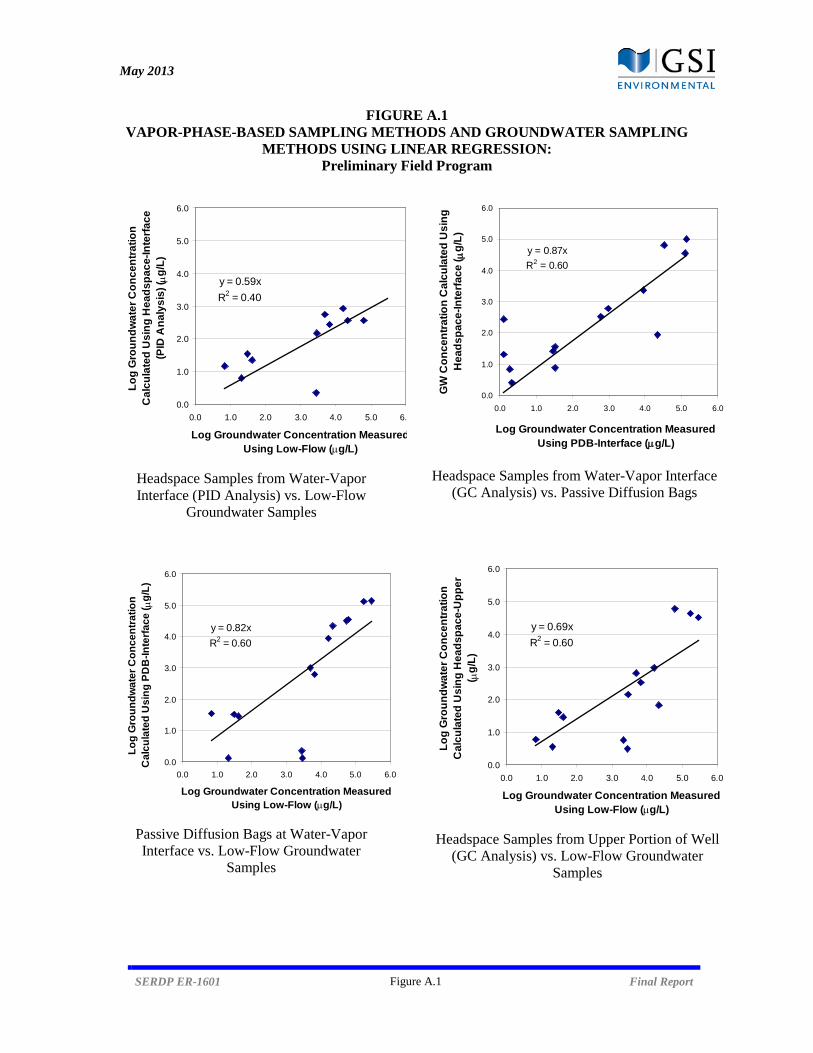
May 2013
FIGURE A.1 VAPOR-PHASE-BASED SAMPLING METHODS AND GROUNDWATER SAMPLING
METHODS USING LINEAR REGRESSION: Preliminary Field Program
SERDP ER-1601 Figure A.1 Final Report
Headspace Samples from Water-Vapor Interface (PID Analysis) vs. Low-Flow
Groundwater Samples
Passive Diffusion Bags at Water-Vapor Interface vs. Low-Flow Groundwater
Samples
Headspace Samples from Water-Vapor Interface (GC Analysis) vs. Passive Diffusion Bags
Headspace Samples from Upper Portion of Well
(GC Analysis) vs. Low-Flow Groundwater Samples
y = 0.59xR2 = 0.40
0.0
1.0
2.0
3.0
4.0
5.0
6.0
0.0 1.0 2.0 3.0 4.0 5.0 6.
Log Groundwater Concentration Measured Using Low-Flow (µg/L)
Lo
g G
rou
nd
wa
ter
Co
nc
en
tra
tio
n
Ca
lcu
late
d U
sin
g H
ea
ds
pa
ce
-In
terf
ac
e
(PID
An
aly
sis
) ( µ
g/L
)
y = 0.82xR2 = 0.60
0.0
1.0
2.0
3.0
4.0
5.0
6.0
0.0 1.0 2.0 3.0 4.0 5.0 6.0
Log Groundwater Concentration Measured Using Low-Flow (µg/L)
Lo
g G
rou
nd
wa
ter
Co
nc
en
tra
tio
n
Ca
lcu
late
d U
sin
g P
DB
-In
terf
ac
e (µg
/L)
y = 0.87xR2 = 0.60
0.0
1.0
2.0
3.0
4.0
5.0
6.0
0.0 1.0 2.0 3.0 4.0 5.0 6.0
Log Groundwater Concentration Measured Using PDB-Interface (µg/L)
GW
Co
nc
en
tra
tio
n C
alc
ula
ted
Us
ing
H
ea
ds
pa
ce
-In
terf
ac
e (µ
g/L
)
y = 0.69xR2 = 0.60
0.0
1.0
2.0
3.0
4.0
5.0
6.0
0.0 1.0 2.0 3.0 4.0 5.0 6.0
Log Groundwater Concentration Measured Using Low-Flow (µg/L)
Lo
g G
rou
nd
wa
ter
Co
nc
en
tra
tio
n
Ca
lcu
late
d U
sin
g H
ea
ds
pa
ce
-Up
pe
r ( µ
g/L
)
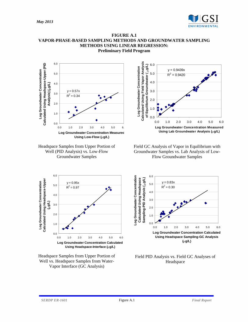
May 2013
FIGURE A.1 VAPOR-PHASE-BASED SAMPLING METHODS AND GROUNDWATER SAMPLING
METHODS USING LINEAR REGRESSION: Preliminary Field Program
SERDP ER-1601 Figure A.1 Final Report
Headspace Samples from Upper Portion of
Well (PID Analysis) vs. Low-Flow Groundwater Samples
Headspace Samples from Upper Portion of Well vs. Headspace Samples from Water-
Vapor Interface (GC Analysis)
Field GC Analysis of Vapor in Equilibrium with Groundwater Samples vs. Lab Analysis of Low-
Flow Groundwater Samples
Field PID Analysis vs. Field GC Analyses of Headspace
y = 0.57xR2 = 0.34
0.0
1.0
2.0
3.0
4.0
5.0
6.0
0.0 1.0 2.0 3.0 4.0 5.0 6.
Log Groundwater Concentration Measured Using Low-Flow (µg/L)
Lo
g G
rou
nd
wa
ter
Co
nc
en
tra
tio
n
Ca
lcu
late
d U
sin
g H
ea
ds
pa
ce
-Up
pe
r (P
ID
An
aly
sis
) ( µ
g/L
)
y = 0.95xR2 = 0.97
0.0
1.0
2.0
3.0
4.0
5.0
6.0
0.0 1.0 2.0 3.0 4.0 5.0 6.0
Log Groundwater Concentration Calculated Using Headspace-Interface (µg/L)
Lo
g G
rou
nd
wa
ter
Co
nc
en
tra
tio
n
Ca
lcu
late
d U
sin
g H
ea
ds
pa
ce
-Up
pe
r ( µ
g/L
)
y = 0.9439xR2 = 0.9420
0.0
1.0
2.0
3.0
4.0
5.0
6.0
0.0 1.0 2.0 3.0 4.0 5.0 6.0
Log Groundwater Concentration Measured Using Lab Groundwater Analysis (µg/L)
Lo
g G
rou
nd
wa
ter
Co
nc
en
tra
tio
n
Ca
lcu
late
d U
sin
g F
ield
Va
po
r A
na
lys
is
of
Eq
uil
ibri
um
Gro
un
dw
ate
r (µg
/L)
y = 0.83xR2 = 0.30
0.0
1.0
2.0
3.0
4.0
5.0
6.0
0.0 1.0 2.0 3.0 4.0 5.0 6.0
Log Groundwater Concentration Calculated Using Headspace Sampling-GC Analysis
(µg/L)
Lo
g G
rou
nd
wa
ter
Co
nc
en
tra
tio
n
Ca
lcu
late
d U
sin
g H
ea
ds
pa
ce
S
am
plin
g-P
ID A
na
lys
is (
µg
/L)
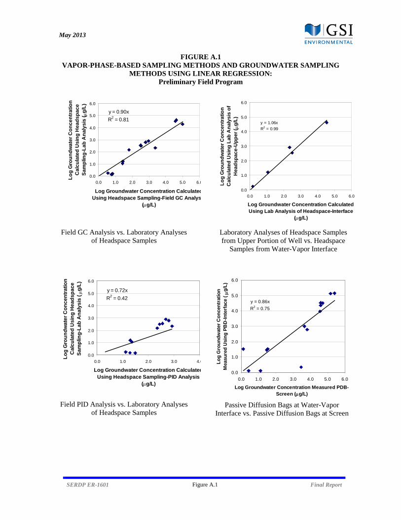
May 2013
FIGURE A.1 VAPOR-PHASE-BASED SAMPLING METHODS AND GROUNDWATER SAMPLING
METHODS USING LINEAR REGRESSION: Preliminary Field Program
SERDP ER-1601 Figure A.1 Final Report
Field GC Analysis vs. Laboratory Analyses of Headspace Samples
Field PID Analysis vs. Laboratory Analyses
of Headspace Samples
Laboratory Analyses of Headspace Samples from Upper Portion of Well vs. Headspace
Samples from Water-Vapor Interface
Passive Diffusion Bags at Water-Vapor
Interface vs. Passive Diffusion Bags at Screen
y = 0.90xR2 = 0.81
0.0
1.0
2.0
3.0
4.0
5.0
6.0
0.0 1.0 2.0 3.0 4.0 5.0 6.0
Log Groundwater Concentration Calculated Using Headspace Sampling-Field GC Analys
(µg/L)
Lo
g G
rou
nd
wa
ter
Co
nc
en
tra
tio
n
Ca
lcu
late
d U
sin
g H
ea
ds
pa
ce
S
am
plin
g-L
ab
An
aly
sis
( µg
/L)
y = 0.72xR2 = 0.42
0.0
1.0
2.0
3.0
4.0
5.0
6.0
0.0 1.0 2.0 3.0 4.0
Log Groundwater Concentration Calculated Using Headspace Sampling-PID Analysis
(µg/L)
Lo
g G
rou
nd
wa
ter
Co
nc
en
tra
tio
n
Ca
lcu
late
d U
sin
g H
ea
ds
pa
ce
S
am
plin
g-L
ab
An
aly
sis
( µ
g/L
)
y = 1.06xR2 = 0.99
0.0
1.0
2.0
3.0
4.0
5.0
6.0
0.0 1.0 2.0 3.0 4.0 5.0 6.0
Log Groundwater Concentration Calculated Using Lab Analysis of Headspace-Interface
(µg/L)L
og
Gro
un
dw
ate
r C
on
ce
ntr
ati
on
C
alc
ula
ted
Us
ing
La
b A
na
lys
is o
f H
ea
ds
pa
ce
-Up
pe
r ( µ
g/L
)
y = 0.86xR2 = 0.75
0.0
1.0
2.0
3.0
4.0
5.0
6.0
0.0 1.0 2.0 3.0 4.0 5.0 6.0
Log Groundwater Concentration Measured PDB-Screen (µg/L)
Lo
g G
rou
nd
wat
er C
on
cen
trat
ion
M
easu
red
Usi
ng
PB
D-I
nte
rfac
e (µg
/L)

May 2013
FIGURE A.2 COMPARISON OF VAPOR-PHASE-BASED SAMPLING METHODS AND
GROUNDWATER SAMPLING METHODS USING LINEAR REGRESSION: Expanded Field Program
SERDP ER-1601 Figure A.2 Final Report
Short Passive Vapor Diffusion (PVD) Samplers vs. Low-Flow Groundwater
Samples
GSI Extended-Length Passive Vapor Diffusion (PVD) Samplers (GC Analysis)
vs. Low-Flow Groundwater Samples
GSI Extended-Length Passive Vapor
Diffusion (PVD) Samplers (PID Analysis) vs. Low-Flow Groundwater Samples
GSI Extended-Length Passive Vapor Diffusion (PVD) Samplers (HAPSITE Analysis) vs. Low-Flow Groundwater
Samples
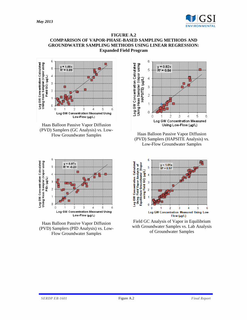
May 2013
FIGURE A.2 COMPARISON OF VAPOR-PHASE-BASED SAMPLING METHODS AND
GROUNDWATER SAMPLING METHODS USING LINEAR REGRESSION: Expanded Field Program
SERDP ER-1601 Figure A.2 Final Report
Haas Balloon Passive Vapor Diffusion
(PVD) Samplers (GC Analysis) vs. Low-Flow Groundwater Samples
Haas Balloon Passive Vapor Diffusion
(PVD) Samplers (PID Analysis) vs. Low-Flow Groundwater Samples
Haas Balloon Passive Vapor Diffusion
(PVD) Samplers (HAPSITE Analysis) vs. Low-Flow Groundwater Samples
Field GC Analysis of Vapor in Equilibrium
with Groundwater Samples vs. Lab Analysis of Groundwater Samples
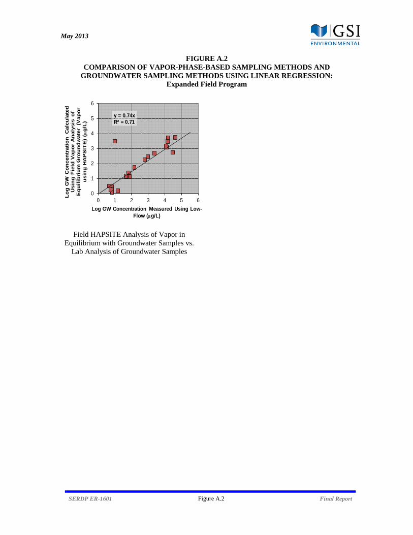
May 2013
FIGURE A.2 COMPARISON OF VAPOR-PHASE-BASED SAMPLING METHODS AND
GROUNDWATER SAMPLING METHODS USING LINEAR REGRESSION: Expanded Field Program
SERDP ER-1601 Figure A.2 Final Report
Field HAPSITE Analysis of Vapor in Equilibrium with Groundwater Samples vs.
Lab Analysis of Groundwater Samples
y = 0.74xR² = 0.71
0
1
2
3
4
5
6
0 1 2 3 4 5 6
Lo
g G
W C
on
cen
trati
on
C
alc
ula
ted
U
sin
g F
ield
Vap
or
An
aly
sis
of
Eq
uil
ibri
um
Gro
un
dw
ate
r (V
ap
or
usin
g H
AP
SIT
E)
(µg
/L)
Log GW Concentration Measured Using Low-Flow (µg/L)
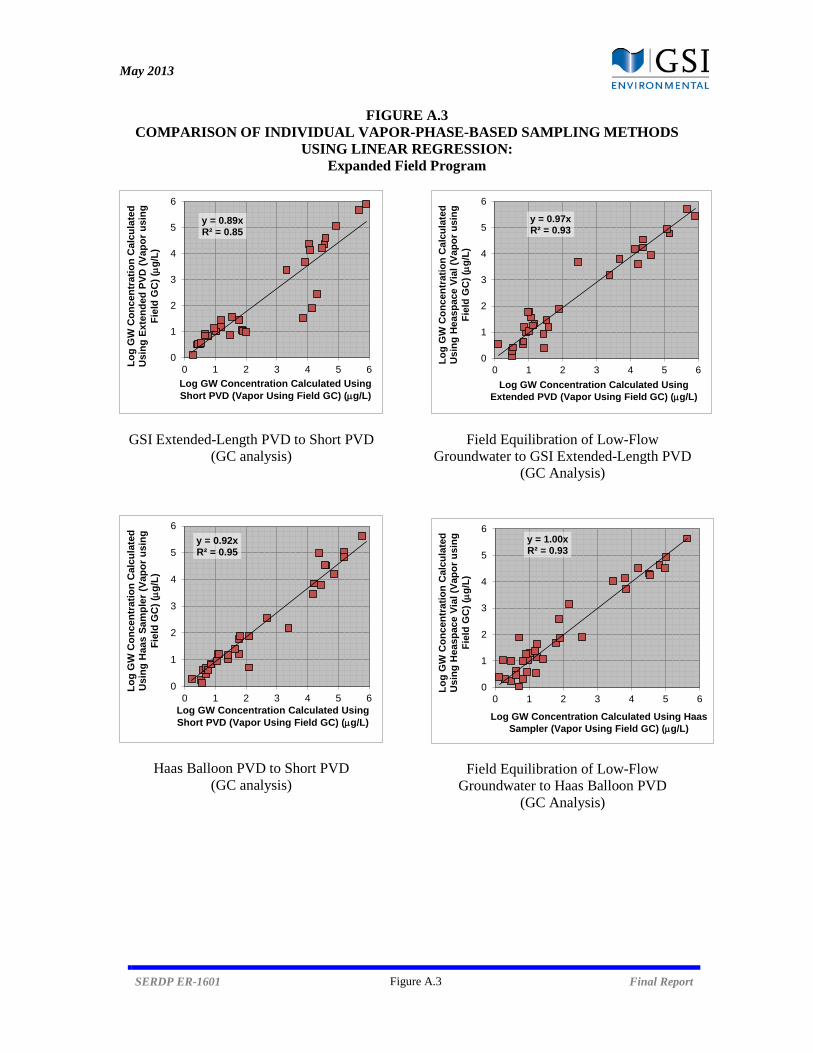
May 2013
FIGURE A.3 COMPARISON OF INDIVIDUAL VAPOR-PHASE-BASED SAMPLING METHODS
USING LINEAR REGRESSION: Expanded Field Program
SERDP ER-1601 Figure A.3 Final Report
GSI Extended-Length PVD to Short PVD (GC analysis)
Haas Balloon PVD to Short PVD (GC analysis)
Field Equilibration of Low-Flow Groundwater to GSI Extended-Length PVD
(GC Analysis)
Field Equilibration of Low-Flow Groundwater to Haas Balloon PVD
(GC Analysis)
y = 0.89xR² = 0.85
0
1
2
3
4
5
6
0 1 2 3 4 5 6Lo
g G
W C
on
cen
trat
ion
Cal
cula
ted
U
sin
g E
xten
ded
PV
D (
Vap
or
usi
ng
F
ield
GC
) (µ
g/L
)
Log GW Concentration Calculated Using Short PVD (Vapor Using Field GC) (µg/L)
y = 0.92xR² = 0.95
0
1
2
3
4
5
6
0 1 2 3 4 5 6
Lo
g G
W C
on
cen
trat
ion
Cal
cula
ted
U
sin
g H
aas
Sam
ple
r (V
apo
r u
sin
g
Fie
ld G
C)
(µg
/L)
Log GW Concentration Calculated Using Short PVD (Vapor Using Field GC) (µg/L)
y = 0.97xR² = 0.93
0
1
2
3
4
5
6
0 1 2 3 4 5 6
Lo
g G
W C
on
cen
trat
ion
Cal
cula
ted
U
sin
g H
easp
ace
Via
l (V
apo
r u
sin
g
Fie
ld G
C)
(µg
/L)
Log GW Concentration Calculated Using Extended PVD (Vapor Using Field GC) (µg/L)
y = 1.00xR² = 0.93
0
1
2
3
4
5
6
0 1 2 3 4 5 6
Lo
g G
W C
on
cen
trat
ion
Cal
cula
ted
U
sin
g H
easp
ace
Via
l (V
apo
r u
sin
g
Fie
ld G
C)
(µg
/L)
Log GW Concentration Calculated Using Haas Sampler (Vapor Using Field GC) (µg/L)
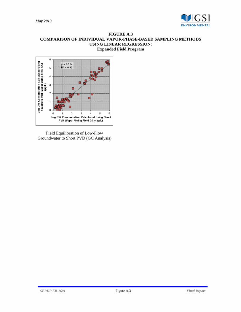
May 2013
FIGURE A.3 COMPARISON OF INDIVIDUAL VAPOR-PHASE-BASED SAMPLING METHODS
USING LINEAR REGRESSION: Expanded Field Program
SERDP ER-1601 Figure A.3 Final Report
Field Equilibration of Low-Flow Groundwater to Short PVD (GC Analysis)
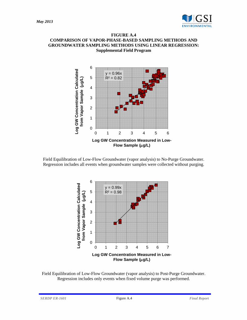
May 2013
FIGURE A.4 COMPARISON OF VAPOR-PHASE-BASED SAMPLING METHODS AND
GROUNDWATER SAMPLING METHODS USING LINEAR REGRESSION: Supplemental Field Program
SERDP ER-1601 Figure A.4 Final Report
Field Equilibration of Low-Flow Groundwater (vapor analysis) to No-Purge Groundwater. Regression includes all events when groundwater samples were collected without purging.
Field Equilibration of Low-Flow Groundwater (vapor analysis) to Post-Purge Groundwater. Regression includes only events when fixed volume purge was performed.
y = 0.96xR² = 0.82
0
1
2
3
4
5
6
0 1 2 3 4 5 6Lo
g G
W C
on
cen
trat
ion
Cal
cula
ted
fr
om
Vap
or
Sam
ple
(µ
g/L
)
Log GW Concentration Measured in Low-Flow Sample (µg/L)
y = 0.99xR² = 0.98
0
1
2
3
4
5
6
0 1 2 3 4 5 6 7Lo
g G
W C
on
cen
trat
ion
Cal
cula
ted
fr
om
Vap
or
Sam
ple
(µ
g/L
)
Log GW Concentration Measured in Low-Flow Sample (µg/L)

May 2013
FIGURE A.4 COMPARISON OF VAPOR-PHASE-BASED SAMPLING METHODS AND
GROUNDWATER SAMPLING METHODS USING LINEAR REGRESSION: Supplemental Field Program
SERDP ER-1601 Figure A.4 Final Report
Field Equilibration of Low-Flow Groundwater (vapor analysis) to Post-Purge Groundwater. Regression includes only events when purge to parameter stability (PPS) was performed.
Field Equilibration of Low-Flow Groundwater (vapor analysis) to Groundwater Collected following In-Well Mixing.
y = 0.97xR² = 0.94
0
1
2
3
4
5
6
0 1 2 3 4 5 6Lo
g G
W C
on
cen
trat
ion
Cal
cula
ted
fr
om
Vap
or
Sam
ple
(µg
/L)
Log GW Concentration Measured in Low-Flow Sample (µg/L)
y = 0.88xR² = 0.70
0
1
2
3
4
5
6
0 1 2 3 4 5 6Lo
g G
W C
on
cen
trat
ion
Cal
cula
ted
fr
om
Vap
or
Sam
ple
(µg
/L)
Log GW Concentration Measured in Low-Flow Sample (µg/L)
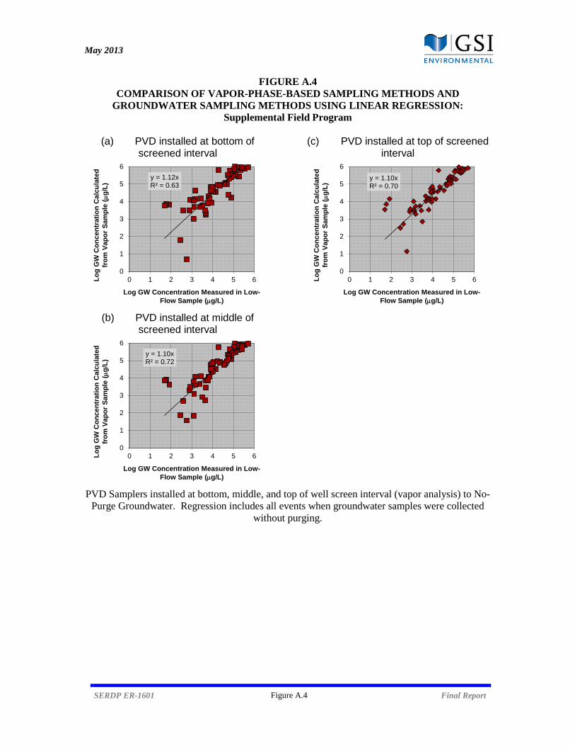
May 2013
FIGURE A.4 COMPARISON OF VAPOR-PHASE-BASED SAMPLING METHODS AND
GROUNDWATER SAMPLING METHODS USING LINEAR REGRESSION: Supplemental Field Program
SERDP ER-1601 Figure A.4 Final Report
(a) PVD installed at bottom of screened interval
(b) PVD installed at middle of
screened interval
(c) PVD installed at top of screened interval
PVD Samplers installed at bottom, middle, and top of well screen interval (vapor analysis) to No-Purge Groundwater. Regression includes all events when groundwater samples were collected
without purging.
y = 1.12xR² = 0.63
0
1
2
3
4
5
6
0 1 2 3 4 5 6Lo
g G
W C
on
cen
trat
ion
Cal
cula
ted
fr
om
Vap
or
Sam
ple
(µg
/L)
Log GW Concentration Measured in Low-Flow Sample (µg/L)
y = 1.10xR² = 0.72
0
1
2
3
4
5
6
0 1 2 3 4 5 6Lo
g G
W C
on
cen
trat
ion
Cal
cula
ted
fr
om
Vap
or
Sam
ple
(µg
/L)
Log GW Concentration Measured in Low-Flow Sample (µg/L)
y = 1.10xR² = 0.70
0
1
2
3
4
5
6
0 1 2 3 4 5 6Lo
g G
W C
on
cen
trat
ion
Cal
cula
ted
fr
om
Vap
or
Sam
ple
(µg
/L)
Log GW Concentration Measured in Low-Flow Sample (µg/L)

May 2013
FIGURE A.4 COMPARISON OF VAPOR-PHASE-BASED SAMPLING METHODS AND
GROUNDWATER SAMPLING METHODS USING LINEAR REGRESSION: Supplemental Field Program
SERDP ER-1601 Figure A.4 Final Report
(d) PVD installed at bottom of screened interval
(e) PVD installed at middle of
screened interval
(f) PVD installed at top of screened interval
PVD Samplers installed at bottom, middle, and top of well screen interval (vapor analysis) to
Post-Purge Groundwater. Regression includes only events when fixed volume purge was performed.
y = 1.10xR² = 0.60
0
1
2
3
4
5
6
0 1 2 3 4 5 6 7Lo
g G
W C
on
cen
trat
ion
Cal
cula
ted
fr
om
Vap
or
Sam
ple
(µg
/L)
Log GW Concentration Measured in Low-Flow Sample (µg/L)
y = 1.08xR² = 0.73
0
1
2
3
4
5
6
0 1 2 3 4 5 6 7Lo
g G
W C
on
cen
trat
ion
Cal
cula
ted
fr
om
Vap
or
Sam
ple
(µg
/L)
Log GW Concentration Measured in Low-Flow Sample (µg/L)
y = 1.07xR² = 0.67
0
1
2
3
4
5
6
0 1 2 3 4 5 6 7Lo
g G
W C
on
cen
trat
ion
Cal
cula
ted
fr
om
Vap
or
Sam
ple
(µg
/L)
Log GW Concentration Measured in Low-Flow Sample (µg/L)
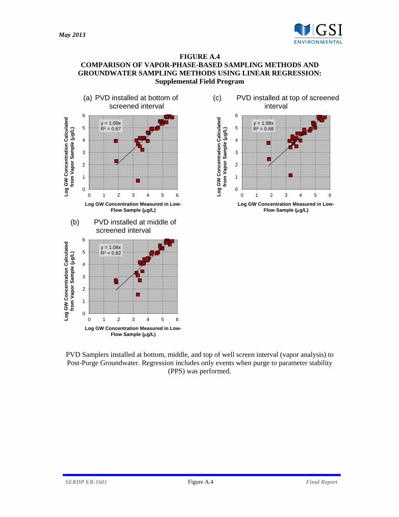
May 2013
FIGURE A.4 COMPARISON OF VAPOR-PHASE-BASED SAMPLING METHODS AND
GROUNDWATER SAMPLING METHODS USING LINEAR REGRESSION: Supplemental Field Program
SERDP ER-1601 Figure A.4 Final Report
(a) PVD installed at bottom of screened interval
(b) PVD installed at middle of
screened interval
(c) PVD installed at top of screened interval
PVD Samplers installed at bottom, middle, and top of well screen interval (vapor analysis) to Post-Purge Groundwater. Regression includes only events when purge to parameter stability
(PPS) was performed.
y = 1.09xR² = 0.67
0
1
2
3
4
5
6
0 1 2 3 4 5 6Lo
g G
W C
on
cen
trat
ion
Cal
cula
ted
fr
om
Vap
or
Sam
ple
(µg
/L)
Log GW Concentration Measured in Low-Flow Sample (µg/L)
y = 1.08xR² = 0.82
0
1
2
3
4
5
6
0 1 2 3 4 5 6Lo
g G
W C
on
cen
trat
ion
Cal
cula
ted
fr
om
Vap
or
Sam
ple
(µg
/L)
Log GW Concentration Measured in Low-Flow Sample (µg/L)
y = 1.08xR² = 0.68
0
1
2
3
4
5
6
0 1 2 3 4 5 6Lo
g G
W C
on
cen
trat
ion
Cal
cula
ted
fr
om
Vap
or
Sam
ple
(µg
/L)
Log GW Concentration Measured in Low-Flow Sample (µg/L)

May 2013
FIGURE A.4 COMPARISON OF VAPOR-PHASE-BASED SAMPLING METHODS AND
GROUNDWATER SAMPLING METHODS USING LINEAR REGRESSION: Supplemental Field Program
SERDP ER-1601 Figure A.4 Final Report
(a) PVD installed at bottom of screened interval
(b) PVD installed at middle of screened interval
(c) PVD installed at middle of screened interval
PVD Samplers installed at bottom, middle, and top of well screen interval (vapor analysis) to
Groundwater Collected using Snap samplers.
y = 1.09xR² = 0.82
0
1
2
3
4
5
6
0 1 2 3 4 5 6Lo
g G
W C
on
cen
trat
ion
Cal
cula
ted
fr
om
Vap
or
Sam
ple
(µg
/L)
Log GW Concentration Measured in Low-Flow Sample (µg/L)
y = 1.08xR² = 0.87
0
1
2
3
4
5
6
0 1 2 3 4 5 6Lo
g G
W C
on
cen
trat
ion
Cal
cula
ted
fr
om
Vap
or
Sam
ple
(µg
/L)
Log GW Concentration Measured in Low-Flow Sample (µg/L)
y = 1.08xR² = 0.84
0
1
2
3
4
5
6
0 1 2 3 4 5 6Lo
g G
W C
on
cen
trat
ion
Cal
cula
ted
fr
om
Vap
or
Sam
ple
(µg
/L)
Log GW Concentration Measured in Low-Flow Sample (µg/L)
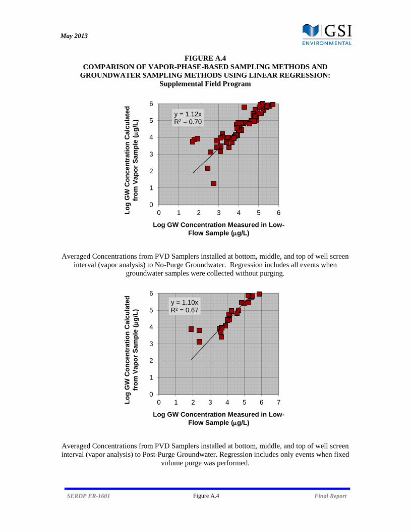
May 2013
FIGURE A.4 COMPARISON OF VAPOR-PHASE-BASED SAMPLING METHODS AND
GROUNDWATER SAMPLING METHODS USING LINEAR REGRESSION: Supplemental Field Program
SERDP ER-1601 Figure A.4 Final Report
Averaged Concentrations from PVD Samplers installed at bottom, middle, and top of well screen interval (vapor analysis) to No-Purge Groundwater. Regression includes all events when
groundwater samples were collected without purging.
Averaged Concentrations from PVD Samplers installed at bottom, middle, and top of well screen interval (vapor analysis) to Post-Purge Groundwater. Regression includes only events when fixed
volume purge was performed.
y = 1.12xR² = 0.70
0
1
2
3
4
5
6
0 1 2 3 4 5 6Lo
g G
W C
on
cen
trat
ion
Cal
cula
ted
fr
om
Vap
or
Sam
ple
(µg
/L)
Log GW Concentration Measured in Low-Flow Sample (µg/L)
y = 1.10xR² = 0.67
0
1
2
3
4
5
6
0 1 2 3 4 5 6 7Lo
g G
W C
on
cen
trat
ion
Cal
cula
ted
fr
om
Vap
or
Sam
ple
(µg
/L)
Log GW Concentration Measured in Low-Flow Sample (µg/L)
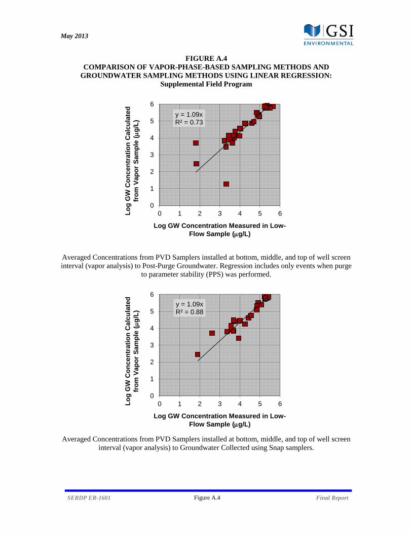
May 2013
FIGURE A.4 COMPARISON OF VAPOR-PHASE-BASED SAMPLING METHODS AND
GROUNDWATER SAMPLING METHODS USING LINEAR REGRESSION: Supplemental Field Program
SERDP ER-1601 Figure A.4 Final Report
Averaged Concentrations from PVD Samplers installed at bottom, middle, and top of well screen interval (vapor analysis) to Post-Purge Groundwater. Regression includes only events when purge
to parameter stability (PPS) was performed.
Averaged Concentrations from PVD Samplers installed at bottom, middle, and top of well screen
interval (vapor analysis) to Groundwater Collected using Snap samplers.
y = 1.09xR² = 0.73
0
1
2
3
4
5
6
0 1 2 3 4 5 6Lo
g G
W C
on
cen
trat
ion
Cal
cula
ted
fr
om
Vap
or
Sam
ple
(µg
/L)
Log GW Concentration Measured in Low-Flow Sample (µg/L)
y = 1.09xR² = 0.88
0
1
2
3
4
5
6
0 1 2 3 4 5 6Lo
g G
W C
on
cen
trat
ion
Cal
cula
ted
fr
om
Vap
or
Sam
ple
(µg
/L)
Log GW Concentration Measured in Low-Flow Sample (µg/L)
May 2013
SERDP ER-1601 Appendix B Final Report
APPENDIX B: LIST OF SCIENTIFIC/TECHNICAL PUBLICATIONS
McHugh, T.E., D.T. Adamson, C.J. Newell, and M. Rysz, 2009. “Vapor-Phase Monitoring of
Groundwater Monitoring Wells: Laboratory Validation”. The Tenth Annual In Situ and On-Site Bioremediation Symposium, Baltimore, MD, May 5, 2009.
Adamson, D.T., T.E. McHugh, M.R. Rysz, and C.J. Newell, 2009. “Laboratory Validation Study of New Vapor-Phase-Based Approach for Groundwater Monitoring”, Remediation, Winter 2009, 20(1): 87-106.
Newell, C.J., T.E. McHugh, D.T. Adamson, and M. Rysz, 2010. “Simplifying Groundwater Sampling: Implications for Long-Term Monitoring Strategies”. Remediation of Chlorinated and Recalcitrant Compounds, The Seventh International Conference, In Situ and On-Site Bioremediation Symposium, Monterey, CA, May 24, 2010.
Adamson, D.T., T.E. McHugh, M.R. Rysz, R.C. Landazuri, and C.J. Newell, 2012. “Field Investigation of Vapor-Phase-Based Groundwater Monitoring”, Ground Water Monitoring & Remediation, Winter 2012, 32(1): 59-72.
Adamson, D.T., C.J. Newell, T.E. McHugh, M. Rysz, R.C. Landazuri, and M.A. Seyedabbasi, 2012. “Field Testing of Vapor-Phase Based Approaches for Monitoring of Groundwater Wells”. Remediation of Chlorinated and Recalcitrant Compounds, The Eighth International Conference, In Situ and On-Site Bioremediation Symposium, Monterey, CA, May 21, 2012.
McHugh, T.E., C.J. Newell, R.C. Landazuri, L.J. Molofsky, and D.T. Adamson, 2012. “The Influence of Seasonal Temperature Gradients on No-Purge Sampling of Wells”, Remediation, Autumn 2012, 22(4): 21-36.
Adamson, D.T., T.E. McHugh, M.R. Rysz, R.C. Landazuri, M.A. Seyedabbasi, P.E. Haas, and C.J. Newell, 2013. “On-Site Vapor-Phase Analysis as a Novel Approach for Monitoring Groundwater Wells”, manuscript in preparation, Spring 2013.

May 2013
SERDP ER-1601 Appendix C Final Report
APPENDIX C: OTHER SUPPORTING MATERIALS
User's Manual
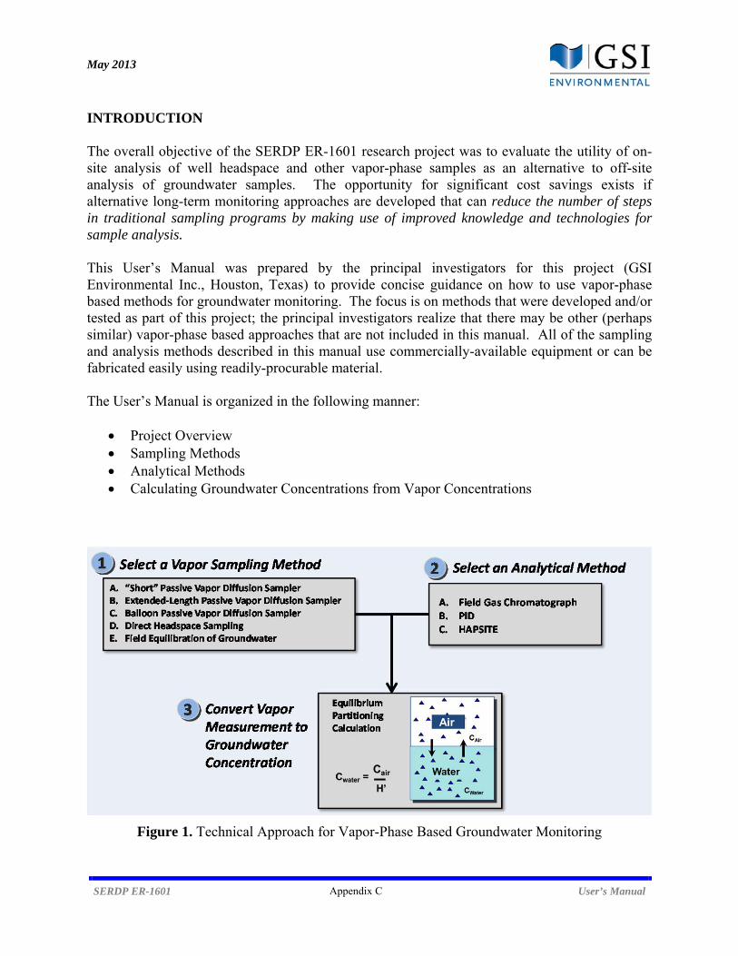
May 2013
SERDP ER-1601 Appendix C User’s Manual
INTRODUCTION The overall objective of the SERDP ER-1601 research project was to evaluate the utility of on-site analysis of well headspace and other vapor-phase samples as an alternative to off-site analysis of groundwater samples. The opportunity for significant cost savings exists if alternative long-term monitoring approaches are developed that can reduce the number of steps in traditional sampling programs by making use of improved knowledge and technologies for sample analysis. This User’s Manual was prepared by the principal investigators for this project (GSI Environmental Inc., Houston, Texas) to provide concise guidance on how to use vapor-phase based methods for groundwater monitoring. The focus is on methods that were developed and/or tested as part of this project; the principal investigators realize that there may be other (perhaps similar) vapor-phase based approaches that are not included in this manual. All of the sampling and analysis methods described in this manual use commercially-available equipment or can be fabricated easily using readily-procurable material. The User’s Manual is organized in the following manner:
Project Overview Sampling Methods Analytical Methods Calculating Groundwater Concentrations from Vapor Concentrations
Figure 1. Technical Approach for Vapor-Phase Based Groundwater Monitoring
May 2013
SERDP ER-1601 Appendix C User’s Manual
PROJECT OVERVIEW Currently, groundwater monitoring programs employed by the DoD (and most non-federal stakeholders) rely heavily on 25 to 30-year old techniques, and must go through multiple steps of collection, handling, lab analysis, and data transfer before the results reach the intended audience. The development of reliable vapor-phase-based monitoring approaches is designed to aid the DoD with several key goals in long-term monitoring optimization. First, it entails a less cost and time-intensive method for analyzing specific contaminants of concern, including all chlorinated hydrocarbons. Further, it can utilize inexpensive and cost-effective tools during the data collection process. Finally, it represents a simple approach that would be easy to implement at a majority of DoD sites nationwide. All of these factors work to significantly reduce the cost liabilities associated with groundwater monitoring while providing a more sustainable long-term approach. The principle driving this research is that the VOC concentration measured in a vapor-phase sample that is in equilibrium with affected groundwater can be used to accurately determine the VOC concentration in the associated groundwater at or below MCLs. Two key hypotheses were developed to support this principle: (1) Portable vapor-phase monitoring instruments can be used to accurately determine VOC concentrations in water under equilibrium conditions; (2) In-well mixing is sufficient in some or all groundwater monitoring wells to establish equilibrium partitioning conditions between affected groundwater and in-well headspace vapors. To test these hypotheses and validate the use of in-field vapor-phase groundwater monitoring techniques, the specific technical objectives of the project were as follows:
1. Validate the use of field-portable vapor phase monitoring equipment to determine VOC concentration in water samples by conducting a detailed laboratory study.
2. Evaluate several different sampling methods to obtain vapor-phase samples in equilibrium with groundwater at the monitoring well.
3. Evaluate the accuracy, precision, and sensitivity of field-based, vapor-phase groundwater monitoring compared to existing groundwater monitoring technologies.
4. Identify conditions where equilibrium partitioning occurs between groundwater and well head space vapors by performing statistical evaluations of the contribution of a variety of aquifer and well construction characteristics to sampling variability.
5. Develop practical guidelines for the selection of appropriate vapor-phase groundwater monitoring strategies for various settings and applications (aquifer type, detection monitoring programs, natural attenuation monitoring programs, etc.), including cost-effectiveness.
Data to address these objectives were collected through a series of testing programs, consisting of: i) a laboratory-based study to validate analytical equipment and to identify promising methods; ii) three distinct phases of field-based studies (preliminary, expanded, and supplemental) to test various sampling and collection methods and to examine design and well-specific factors that influenced performance; and iii) a combined modeling-field study that
May 2013
SERDP ER-1601 Appendix C User’s Manual
focused on the influence of seasonal temperature gradients on vertical stratification of concentration within monitoring wells. The findings (described fully in the SERDP ER-1601 final report) demonstrate that, collectively, the project met all of the stated objectives. Of the original hypotheses, the first hypothesis—that portable vapor-phase monitoring instruments can be used to accurately determine VOC concentrations in water under equilibrium conditions—was validated by the project findings. However, the second hypothesis—that in-well mixing occurs at a high enough frequency to merit the use of headspace sampling—was not entirely validated by the project data. Instead, submerged passive samplers, or an alternative field equilibration method, were demonstrated to be the most appropriate vapor-phase-based methods in most cases. Headspace sampling should be considered a more niche application. These approaches can be tailored for sites where a typical flow-weighted average concentration is desired, or for sites where depth-discrete concentration data are preferred. Any monitoring program that incorporates vapor-phase monitoring should be designed to address whichever of these objectives are appropriate for a given site and monitoring period. For example, the results of the temperature study demonstrated thattemperature gradients within wells can induce mixing or favor stratification, and the prevalent condition depends on the climate, season, and the depth of the well. Shallow wells are much more prone to these temperature effects, while they may be minimal in deeper wells (greater than approximately 15 to 20 m bgs).

May 2013
SERDP ER-1601 Appendix C User’s Manual
SAMPLING METHODS Five different sampling methods were tested as part of this project. The following tables provide an overview of each method, information on deployment, and the relative pros and cons.
1. SHORT PASSIVE VAPOR DIFFUSION (PVD) SAMPLER
Principle Diffusion and equilibrium partitioning
Description The short PVD samplers (based on an earlier USGS design (2002)) are gas-filled containers wrapped in a semi-permeable membrane that are submerged within an aqueous phase. Vapor-phase contaminants are quantified following equilibrium partitioning of contaminants that diffuse across the water-tight but gas permeable membrane that covers the opening of the containers. The short PVD samplers consist of an uncapped 40-mL VOA vial enclosed in an inner layer of heat-sealed lay-flat low-density polyethylene (LDPE). A second protective layer of heat-sealed LDPE should also be used as a protective layer for the sampler. During sampler preparation, care should be taken to evacuate air from inside of both layers to the extent possible.
How to Deploy and Sample
Deployment of the short PVD in groundwater monitoring wells can use either single depth or multi-level configurations. For single PVD installations, the sampler would typically be placed at a depth corresponding to the middle of the monitoring well screen. For multi-level deployment, the samplers can be installed at depth intervals of interest (e.g., top, middle, and/or bottom of the well screens). Sampler installation involves attaching a nylon string to a well cap and securing the PVD(s) to this string with standard 4” cable ties (“zip-ties”) at pre-determined depth targeting the monitoring well screen zone. To prevent the samplers from floating up to the water surface within the well, fisherman weight sinkers should be attached to the bottom of the nylon string (approximately 100 g was used at each well during SERDP ER-1601). Following installation, the PVD samplers equilibrate for a period of several weeks, after which they are collected by opening the well cap and slowly retrieving the nylon string to the surface. After retrieval of the PVD samplers from the wells, the outer protective LDPE membrane is removed and a Teflon-septa cap is placed on the vial neck over the inner LDPE diffusion membrane. This approach ensures that the vapor contents of the sampler are not compromised during retrieval (outer membrane) and that no dilution with ambient air occurs during the preparation of the sampler for analyses (inner membrane). Vapor samples are then collected into a gas-tight syringe by puncturing the Teflon-septa cap for on-site analysis.
Period of Deployment 1 – 4 weeks to allow equilibration (shorter times may be justifiable based on site-specific tests and detailed calculations)
New samplers can be installed immediately after analyzing previous set of samplers
Advantages Robust and not prone to failure
Simple and cheap to construct using readily-available materials
Small – can be installed at multiple depths within the same well
Relatively accurate and precise
Disadvantages Time required for equilibration
One extra mobilization is required at start of monitoring program to install first set of samplers (new samplers can be installed during subsequent monitoring events)
Small sample volume (40-mL) may limit type of analytical equipment that can be used to analyze sample
Small cross-sectional area for diffusion increases required equilibration time (only the vial opening allows diffusion across the membrane)
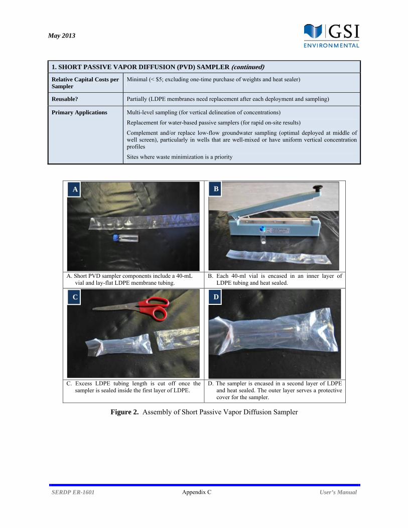
May 2013
SERDP ER-1601 Appendix C User’s Manual
1. SHORT PASSIVE VAPOR DIFFUSION (PVD) SAMPLER (continued)
Relative Capital Costs per Sampler
Minimal (< $5; excluding one-time purchase of weights and heat sealer)
Reusable? Partially (LDPE membranes need replacement after each deployment and sampling)
Primary Applications Multi-level sampling (for vertical delineation of concentrations)
Replacement for water-based passive samplers (for rapid on-site results)
Complement and/or replace low-flow groundwater sampling (optimal deployed at middle of well screen), particularly in wells that are well-mixed or have uniform vertical concentration profiles
Sites where waste minimization is a priority
A. Short PVD sampler components include a 40-mL vial and lay-flat LDPE membrane tubing.
B. Each 40-ml vial is encased in an inner layer of LDPE tubing and heat sealed.
C. Excess LDPE tubing length is cut off once the sampler is sealed inside the first layer of LDPE.
D. The sampler is encased in a second layer of LDPE and heat sealed. The outer layer serves a protective cover for the sampler.
Figure 2. Assembly of Short Passive Vapor Diffusion Sampler
A B
C D
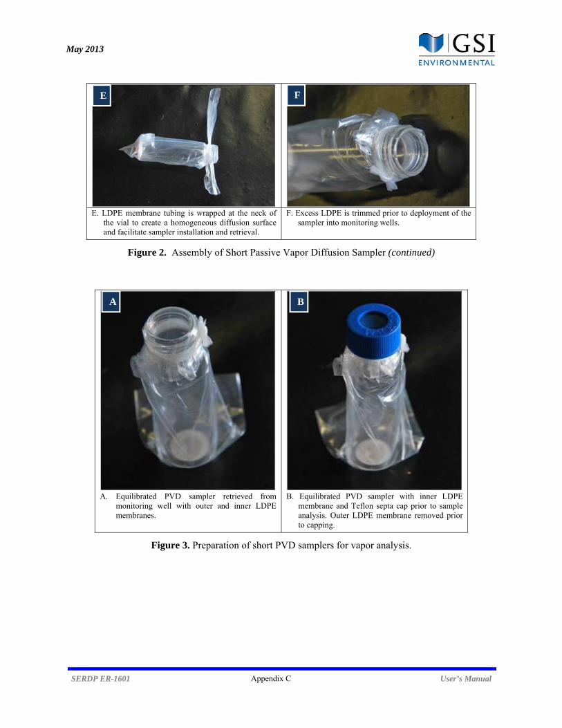
May 2013
SERDP ER-1601 Appendix C User’s Manual
E. LDPE membrane tubing is wrapped at the neck of the vial to create a homogeneous diffusion surface and facilitate sampler installation and retrieval.
F. Excess LDPE is trimmed prior to deployment of the sampler into monitoring wells.
Figure 2. Assembly of Short Passive Vapor Diffusion Sampler (continued)
A. Equilibrated PVD sampler retrieved from monitoring well with outer and inner LDPE membranes.
B. Equilibrated PVD sampler with inner LDPE membrane and Teflon septa cap prior to sample analysis. Outer LDPE membrane removed prior to capping.
Figure 3. Preparation of short PVD samplers for vapor analysis.
A B
E F
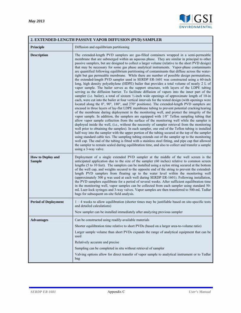
May 2013
SERDP ER-1601 Appendix C User’s Manual
2. EXTENDED-LENGTH PASSIVE VAPOR DIFFUSION (PVD) SAMPLER
Principle Diffusion and equilibrium partitioning
Description The extended-length PVD samplers are gas-filled containers wrapped in a semi-permeable membrane that are submerged within an aqueous phase. They are similar in principal to other passive samplers, but are designed to collect a larger volume (relative to the short PVD design) that may be necessary for some gas phase analytical instruments. Vapor-phase contaminants are quantified following equilibrium partitioning of contaminants that diffuse across the water-tight but gas permeable membrane. While there are number of possible design permutations, the extended-length PVD sampler used in SERDP ER-1601 was constructed using a 60-inch long, high density polyethylene (HDPE) bailer that provides a total volume of nearly 2 L of vapor sample. The bailer serves as the support structure, with layers of the LDPE tubing serving as the diffusion barrier. To facilitate diffusion of vapors into the inner part of the sampler (i.e. bailer), a total of sixteen ½-inch wide openings of approximate length of 10-in each, were cut into the bailer at four vertical intervals for the tested design (with openings were located along the 0°, 90°, 180°, and 270° positions). The extended-length PVD samplers are encased in three layers of lay-flat LDPE membrane tubing to prevent potential cracking/tearing of the membrane during deployment in the monitoring well, and protect the integrity of the vapor sample. In addition, the samplers are equipped with 1/8” Teflon sampling tubing that allow vapor sample collection from the surface of the monitoring well while the sampler is deployed inside the well, (i.e., without the necessity of sampler retrieval from the monitoring well prior to obtaining the samples). In each sampler, one end of the Teflon tubing is installed half-way into the sampler with the upper portion of the tubing secured at the top of the sampler using standard cable ties. The sampling tubing extends out of the sampler up to the monitoring well cap. The end of the tubing is fitted with a stainless steel fitting, and pipe cap that allowed the sampler to remain sealed during equilibration time, and also to collect and transfer a sample using a 3-way valve.
How to Deploy and Sample
Deployment of a single extended PVD sampler at the middle of the well screen is the anticipated application due to the size of the sampler (60 inches) relative to common screen lengths (5 to 10 feet). The samplers can be installed using a nylon string secured at the bottom of the well cap, and weights secured to the opposite end of the string to prevent the extended-length PVD samplers from floating up to the water level within the monitoring well (approximately 300 g was used at each well during SERDP ER-1601). Following installation, the PVD samplers equilibrate for a period of several weeks. After sufficient equilibration time in the monitoring well, vapor samples can be collected from each sampler using standard 50-mL Luer-lock syringes and 3-way valves. Vapor samples are then transferred to 500-mL Tedlar bags for subsequent on-site field analysis.
Period of Deployment 1 – 4 weeks to allow equilibration (shorter times may be justifiable based on site-specific tests and detailed calculations)
New sampler can be installed immediately after analyzing previous sampler
Advantages Can be constructed using readily-available materials
Shorter equilibration time relative to short PVDs (based on a larger area-to-volume ratio)
Larger sample volume than short PVDs expands the range of analytical equipment that can be used
Relatively accurate and precise
Sampling can be completed in situ without retrieval of sampler
Valving options allow for direct transfer of vapor sample to analytical instrument or to Tedlar bag

May 2013
SERDP ER-1601 Appendix C User’s Manual
2. EXTENDED-LENGTH PASSIVE VAPOR DIFFUSION (PVD) SAMPLER (continued)
Disadvantages Time required for equilibration
Not as robust as short PVDs and more prone to failure (e.g., leaking, collapse)
One extra mobilization is required at start of monitoring program to install first set of samplers (new samplers can be installed during subsequent monitoring events)
More complicated and time-consuming to construct than short PVDs
Too large for to allow installation at multiple depths in most wells
Relative Capital Costs per Sampler
Low (< $10; excluding one-time purchase of weights)
Reusable? Yes (assuming diffusion surface is relatively clean – otherwise outer plastic layer should be replaced; sampler retrieval and inspection is recommended if samplers are reused)
Primary Applications Replacement for water-based passive samplers (for rapid on-site results)
Complement and/or replace low-flow groundwater sampling (optimally deployed at middle of well screen), particularly in wells that are not well-mixed or have non-uniform vertical concentration profiles
Sites where waste minimization is a priority
A. 60-in HDPE bailer used as inner structure of the sampler.
B. Installation of Teflon tubing inside the 60-in HDPE bailer.
C. 10-in openings cut out along the four quadrants of the circumference of the bailer to increase cross-sectional area for diffusion.
D. Wrapping sampler with three layers of LDPE membrane.
Figure 4. Assembly of Extended-Length Passive Vapor Diffusion Sampler
A B
C D
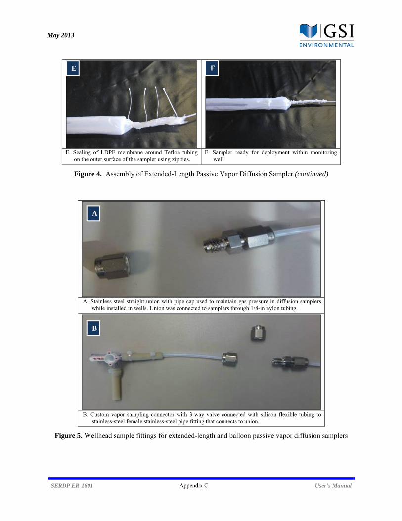
May 2013
SERDP ER-1601 Appendix C User’s Manual
E. Sealing of LDPE membrane around Teflon tubing on the outer surface of the sampler using zip ties.
F. Sampler ready for deployment within monitoring well.
Figure 4. Assembly of Extended-Length Passive Vapor Diffusion Sampler (continued)
A. Stainless steel straight union with pipe cap used to maintain gas pressure in diffusion samplers
while installed in wells. Union was connected to samplers through 1/8-in nylon tubing.
B. Custom vapor sampling connector with 3-way valve connected with silicon flexible tubing to
stainless-steel female stainless-steel pipe fitting that connects to union.
Figure 5. Wellhead sample fittings for extended-length and balloon passive vapor diffusion samplers
A
B
E F
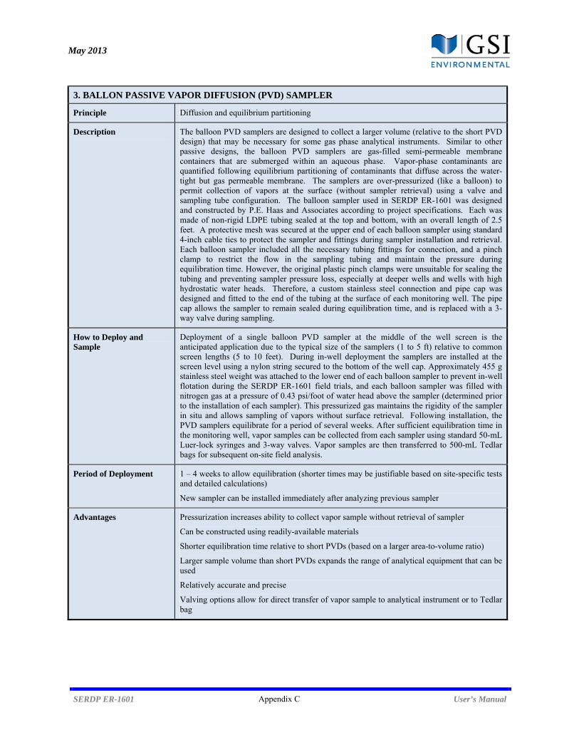
May 2013
SERDP ER-1601 Appendix C User’s Manual
3. BALLON PASSIVE VAPOR DIFFUSION (PVD) SAMPLER
Principle Diffusion and equilibrium partitioning
Description The balloon PVD samplers are designed to collect a larger volume (relative to the short PVD design) that may be necessary for some gas phase analytical instruments. Similar to other passive designs, the balloon PVD samplers are gas-filled semi-permeable membrane containers that are submerged within an aqueous phase. Vapor-phase contaminants are quantified following equilibrium partitioning of contaminants that diffuse across the water-tight but gas permeable membrane. The samplers are over-pressurized (like a balloon) to permit collection of vapors at the surface (without sampler retrieval) using a valve and sampling tube configuration. The balloon sampler used in SERDP ER-1601 was designed and constructed by P.E. Haas and Associates according to project specifications. Each was made of non-rigid LDPE tubing sealed at the top and bottom, with an overall length of 2.5 feet. A protective mesh was secured at the upper end of each balloon sampler using standard 4-inch cable ties to protect the sampler and fittings during sampler installation and retrieval. Each balloon sampler included all the necessary tubing fittings for connection, and a pinch clamp to restrict the flow in the sampling tubing and maintain the pressure during equilibration time. However, the original plastic pinch clamps were unsuitable for sealing the tubing and preventing sampler pressure loss, especially at deeper wells and wells with high hydrostatic water heads. Therefore, a custom stainless steel connection and pipe cap was designed and fitted to the end of the tubing at the surface of each monitoring well. The pipe cap allows the sampler to remain sealed during equilibration time, and is replaced with a 3-way valve during sampling.
How to Deploy and Sample
Deployment of a single balloon PVD sampler at the middle of the well screen is the anticipated application due to the typical size of the samplers (1 to 5 ft) relative to common screen lengths (5 to 10 feet). During in-well deployment the samplers are installed at the screen level using a nylon string secured to the bottom of the well cap. Approximately 455 g stainless steel weight was attached to the lower end of each balloon sampler to prevent in-well flotation during the SERDP ER-1601 field trials, and each balloon sampler was filled with nitrogen gas at a pressure of 0.43 psi/foot of water head above the sampler (determined prior to the installation of each sampler). This pressurized gas maintains the rigidity of the sampler in situ and allows sampling of vapors without surface retrieval. Following installation, the PVD samplers equilibrate for a period of several weeks. After sufficient equilibration time in the monitoring well, vapor samples can be collected from each sampler using standard 50-mL Luer-lock syringes and 3-way valves. Vapor samples are then transferred to 500-mL Tedlar bags for subsequent on-site field analysis.
Period of Deployment 1 – 4 weeks to allow equilibration (shorter times may be justifiable based on site-specific tests and detailed calculations)
New sampler can be installed immediately after analyzing previous sampler
Advantages Pressurization increases ability to collect vapor sample without retrieval of sampler
Can be constructed using readily-available materials
Shorter equilibration time relative to short PVDs (based on a larger area-to-volume ratio)
Larger sample volume than short PVDs expands the range of analytical equipment that can be used
Relatively accurate and precise
Valving options allow for direct transfer of vapor sample to analytical instrument or to Tedlar bag

May 2013
SERDP ER-1601 Appendix C User’s Manual
3. BALLON PASSIVE VAPOR DIFFUSION (PVD) SAMPLER (continued)
Disadvantages Time required for equilibration
Not as robust as short PVDs and more prone to failure (e.g., leaking, collapse)
One extra mobilization is required at start of monitoring program to install first set of samplers (new samplers can be installed during subsequent monitoring events)
More complicated and time-consuming to construct than short PVDs
Too large for to allow installation at multiple depths in most wells
Relative Capital Costs per Sampler
Low (< $20; excluding one-time purchase of weights)
Reusable? Yes (assuming diffusion surface is relatively clean; sampler retrieval and inspection is recommended if samplers are reused)
Primary Applications Replacement for water-based passive samplers (for rapid on-site results)
Complement and/or replace low-flow groundwater sampling (optimally deployed at middle of well screen), particularly in wells that are not well-mixed or have non-uniform vertical concentration profiles
Sites where waste minimization is a priority
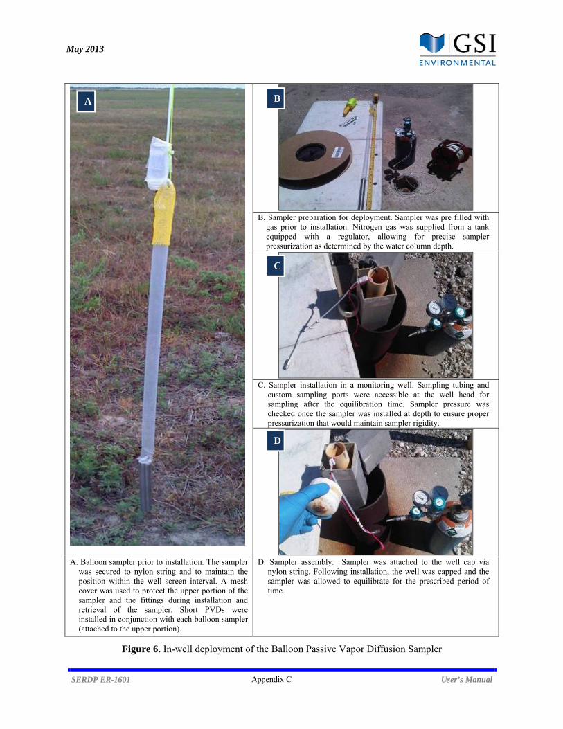
May 2013
SERDP ER-1601 Appendix C User’s Manual
B. Sampler preparation for deployment. Sampler was pre filled with gas prior to installation. Nitrogen gas was supplied from a tank equipped with a regulator, allowing for precise sampler pressurization as determined by the water column depth.
C. Sampler installation in a monitoring well. Sampling tubing and custom sampling ports were accessible at the well head for sampling after the equilibration time. Sampler pressure was checked once the sampler was installed at depth to ensure proper pressurization that would maintain sampler rigidity.
A. Balloon sampler prior to installation. The sampler was secured to nylon string and to maintain the position within the well screen interval. A mesh cover was used to protect the upper portion of the sampler and the fittings during installation and retrieval of the sampler. Short PVDs were installed in conjunction with each balloon sampler (attached to the upper portion).
D. Sampler assembly. Sampler was attached to the well cap via nylon string. Following installation, the well was capped and the sampler was allowed to equilibrate for the prescribed period of time.
Figure 6. In-well deployment of the Balloon Passive Vapor Diffusion Sampler
B
C
D
A
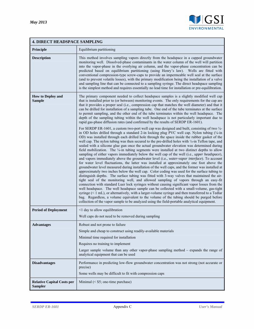
May 2013
SERDP ER-1601 Appendix C User’s Manual
4. DIRECT HEADSPACE SAMPLING
Principle Equilibrium partitioning
Description This method involves sampling vapors directly from the headspace in a capped groundwater monitoring well. Dissolved-phase contaminants in the water column of the well will partition into the vapor-phase in the overlying air column, and the vapor-phase concentration can be predicted based on equilibrium partitioning (using Henry’s law). Wells are fitted with conventional compression-type screw-caps to provide an impermeable well seal at the surface (and to prevent volatile losses), with the primary modification being the installation of a valve and sampling line that can be connected to a sampling syringe. The direct headspace sampling is the simplest method and requires essentially no lead time for installation or pre-equilibration.
How to Deploy and Sample
The primary component needed to collect headspace samples is a slightly modified well cap that is installed prior to (or between) monitoring events. The only requirements for the cap are that it provides a proper seal (i.e., compression cap that matches the well diameter) and that it can be drilled for installation of a sampling tube. One end of the tube terminates at the surface to permit sampling, and the other end of the tube terminates within the well headspace. The depth of the sampling tubing within the well headspace is not particularly important due to rapid gas-phase diffusion rates (and confirmed by the results of SERDP ER-1601).
For SERDP ER-1601, a custom two-port well cap was designed and built, consisting of two ⅛-in OD holes drilled through a standard 2-in locking plug PVC well cap. Nylon tubing (⅛-in OD) was installed through each drilled hole through the space inside the rubber gasket of the well cap. The nylon tubing was then secured to the pre-drilled holes with ¼-in Teflon tape, and sealed with a silicone glue gun once the actual groundwater elevation was determined during field mobilization. The ⅛-in tubing segments were installed at two distinct depths to allow sampling of either vapors immediately below the well cap of the well (i.e., upper headspace), and vapors immediately above the groundwater level (i.e., water-vapor interface). To account for water level fluctuations, the latter was installed at approximately one foot above the groundwater level measured during installation of the well caps, and the former was installed at approximately two inches below the well cap. Color coding was used for the surface tubing to distinguish depths. The surface tubing was fitted with 3-way valves that maintained the air-tight seal of the monitoring well, and allowed sampling of vapors through an easy-fit connection with standard Luer lock syringes without causing significant vapor losses from the well headspace. The well headspace sample can be collected with a small-volume, gas-tight syringe (< 1 mL), or alternatively, with a larger-volume syringe and then transferred to a Tedlar bag. Regardless, a volume equivalent to the volume of the tubing should be purged before collection of the vapor sample to be analyzed using the field-portable analytical equipment.
Period of Deployment <1 day to allow equilibration
Well caps do not need to be removed during sampling
Advantages Robust and not prone to failure
Simple and cheap to construct using readily-available materials
Minimal time required for installation
Requires no training to implement
Larger sample volume than any other vapor-phase sampling method – expands the range of analytical equipment that can be used
Disadvantages Performance in predicting low-flow groundwater concentration was not strong (not accurate or precise)
Some wells may be difficult to fit with compression caps
Relative Capital Costs per Sampler
Minimal (< $5; one-time purchase)
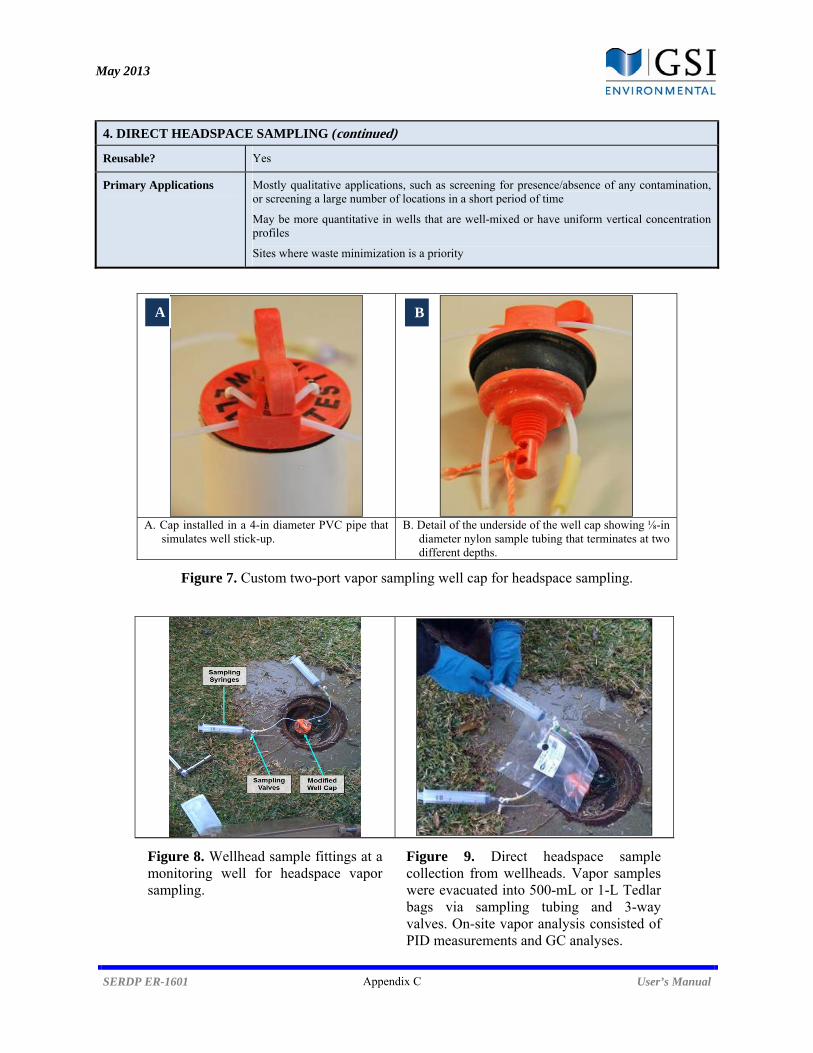
May 2013
SERDP ER-1601 Appendix C User’s Manual
4. DIRECT HEADSPACE SAMPLING (continued)
Reusable? Yes
Primary Applications Mostly qualitative applications, such as screening for presence/absence of any contamination, or screening a large number of locations in a short period of time
May be more quantitative in wells that are well-mixed or have uniform vertical concentration profiles
Sites where waste minimization is a priority
A. Cap installed in a 4-in diameter PVC pipe that
simulates well stick-up. B. Detail of the underside of the well cap showing ⅛-in
diameter nylon sample tubing that terminates at two different depths.
Figure 7. Custom two-port vapor sampling well cap for headspace sampling.
Figure 8. Wellhead sample fittings at a monitoring well for headspace vapor sampling.
Figure 9. Direct headspace sample collection from wellheads. Vapor samples were evacuated into 500-mL or 1-L Tedlar bags via sampling tubing and 3-way valves. On-site vapor analysis consisted of PID measurements and GC analyses.
A B
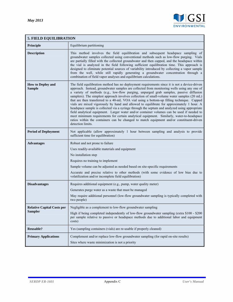
May 2013
SERDP ER-1601 Appendix C User’s Manual
5. FIELD EQUILIBRATION
Principle Equilibrium partitioning
Description This method involves the field equilibration and subsequent headspace sampling of groundwater samples collected using conventional methods such as low-flow purging. Vials are partially filled with the collected groundwater and then capped, and the headspace within the vial is analyzed in the field following sufficient equilibration time. This approach is designed to eliminate potential sources of variability introduced by collecting a vapor sample from the well, while still rapidly generating a groundwater concentration through a combination of field vapor analyses and equilibrium calculations.
How to Deploy and Sample
The field equilibration method has no deployment requirements since it is not a device-driven approach. Instead, groundwater samples are collected from monitoring wells using any one of a variety of methods (e.g., low-flow purging, unpurged grab samples, passive diffusion samplers). The simplest approach involves collection of small-volume water samples (20 mL) that are then transferred to a 40-mL VOA vial using a bottom-up filling technique. Capped vials are mixed vigorously by hand and allowed to equilibrate for approximately 1 hour. A headspace sample is collected via a syringe through the septum and analyzed using appropriate field analytical equipment. Larger water and/or container volumes can be used if needed to meet minimum requirements for certain analytical equipment. Similarly, water-to-headspace ratios within the containers can be changed to match equipment and/or constituent-driven detection limits.
Period of Deployment Not applicable (allow approximately 1 hour between sampling and analysis to provide sufficient time for equilibration)
Advantages Robust and not prone to failure
Uses readily-available materials and equipment
No installation step
Requires no training to implement
Sample volume can be adjusted as needed based on site-specific requirements
Accurate and precise relative to other methods (with some evidence of low bias due to volatilization and/or incomplete field equilibration)
Disadvantages Requires additional equipment (e.g., pump, water quality meter)
Generates purge water as a waste that must be managed
May require additional personnel (low-flow groundwater sampling is typically completed with two people)
Relative Capital Costs per Sampler
Negligible as a complement to low-flow groundwater sampling
High if being completed independently of low-flow groundwater sampling (extra $100 - $200 per sample relative to passive or headspace methods due to additional labor and equipment costs)
Reusable? Yes (sampling containers (vials) are re-usable if properly cleaned)
Primary Applications Complement and/or replace low-flow groundwater sampling (for rapid on-site results)
Sites where waste minimization is not a priority
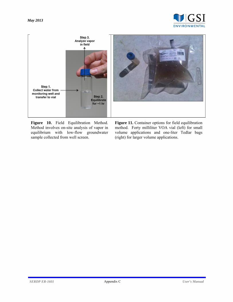
May 2013
SERDP ER-1601 Appendix C User’s Manual
Figure 10. Field Equilibration Method. Method involves on-site analysis of vapor in equilibrium with low-flow groundwater sample collected from well screen.
Figure 11. Container options for field equilibration method. Forty milliliter VOA vial (left) for small volume applications and one-liter Tedlar bags (right) for larger volume applications.
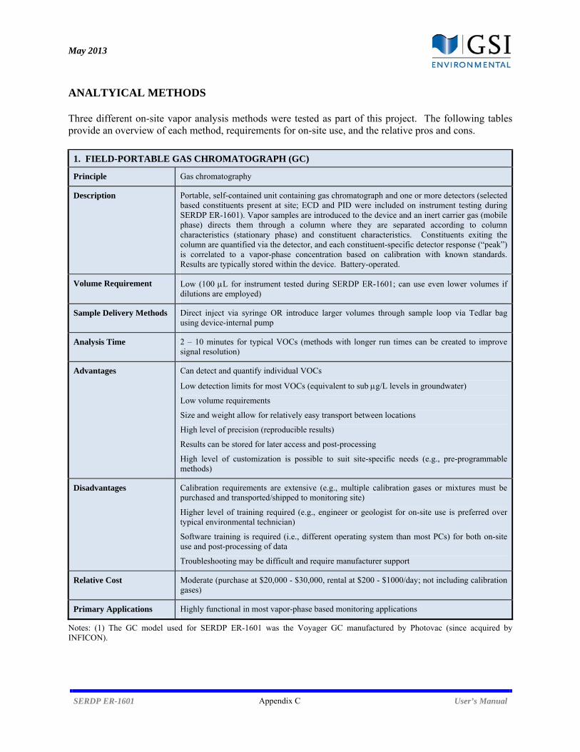
May 2013
SERDP ER-1601 Appendix C User’s Manual
ANALTYICAL METHODS Three different on-site vapor analysis methods were tested as part of this project. The following tables provide an overview of each method, requirements for on-site use, and the relative pros and cons.
1. FIELD-PORTABLE GAS CHROMATOGRAPH (GC)
Principle Gas chromatography
Description Portable, self-contained unit containing gas chromatograph and one or more detectors (selected based constituents present at site; ECD and PID were included on instrument testing during SERDP ER-1601). Vapor samples are introduced to the device and an inert carrier gas (mobile phase) directs them through a column where they are separated according to column characteristics (stationary phase) and constituent characteristics. Constituents exiting the column are quantified via the detector, and each constituent-specific detector response (“peak”) is correlated to a vapor-phase concentration based on calibration with known standards. Results are typically stored within the device. Battery-operated.
Volume Requirement Low (100 L for instrument tested during SERDP ER-1601; can use even lower volumes if dilutions are employed)
Sample Delivery Methods Direct inject via syringe OR introduce larger volumes through sample loop via Tedlar bag using device-internal pump
Analysis Time 2 – 10 minutes for typical VOCs (methods with longer run times can be created to improve signal resolution)
Advantages Can detect and quantify individual VOCs
Low detection limits for most VOCs (equivalent to sub g/L levels in groundwater)
Low volume requirements
Size and weight allow for relatively easy transport between locations
High level of precision (reproducible results)
Results can be stored for later access and post-processing
High level of customization is possible to suit site-specific needs (e.g., pre-programmable methods)
Disadvantages Calibration requirements are extensive (e.g., multiple calibration gases or mixtures must be purchased and transported/shipped to monitoring site)
Higher level of training required (e.g., engineer or geologist for on-site use is preferred over typical environmental technician)
Software training is required (i.e., different operating system than most PCs) for both on-site use and post-processing of data
Troubleshooting may be difficult and require manufacturer support
Relative Cost Moderate (purchase at $20,000 - $30,000, rental at $200 - $1000/day; not including calibration gases)
Primary Applications Highly functional in most vapor-phase based monitoring applications
Notes: (1) The GC model used for SERDP ER-1601 was the Voyager GC manufactured by Photovac (since acquired by INFICON).
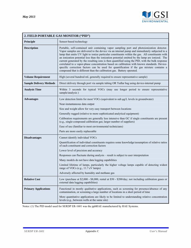
May 2013
SERDP ER-1601 Appendix C User’s Manual
2. FIELD-PORTABLE GAS MONITOR (“PID”)
Principle Sensor-based technology
Description Portable, self-contained unit containing vapor sampling port and photoionization detector. Vapor samples are delivered to the device via an internal pump and immediately subjected to a lamp that emits UV light to ionize particular constituents within the gas. All constituents with an ionization potential less than the ionization potential emitted by the lamp are ionized. The current generated by the resulting ions is then quantified using the PID, with the bulk response correlated to a vapor-phase concentration based on calibration with known standards. Device-specific correction factors can be used for quantification if the gas mixture contains a compound that is different than the calibration gas. Battery operated.
Volume Requirement High (several hundred mL generally required to ensure representative sample)
Sample Delivery Methods Direct delivery through port via sample tubing OR Tedlar bag using device-internal pump
Analysis Time Within 3 seconds for typical VOCs (may use longer period to ensure representative sample/analysis )
Advantages Low detection limits for most VOCs (equivalent to sub μg/L levels in groundwater)
Near-instantaneous data output
Size and weight allow for very easy transport between locations
Generally rugged (relative to more sophisticated analytical equipment)
Calibration requirements are generally less intensive than GC if single constituents are present (e.g., single-compound calibration gas; larger number of suppliers)
Ease of use (familiar to most environmental technicians)
Parts are more easily replaceable
Disadvantages Cannot identify individual VOCs
Quantification of individual constituents requires some knowledge/assumption of relative ratios of each constituent and correction factors
Lower level of precision and accuracy
Responses can fluctuate during analysis – result is subject to user interpretation
Many models do not have data logging capabilities
Limited lifetime of lamps, particularly the higher voltage lamps capable of detecting widest range of VOCs (e.g., 11.7 eV lamps)
Adversely affected by humidity and methane gas
Relative Cost Low (purchase at $2,000 - $8,000, rental at $50 - $200/day; not including calibration gases or external data logging capabilities)
Primary Applications Functional in mostly qualitative applications, such as screening for presence/absence of any contamination, or screening a large number of locations in a short period of time
More quantitative applications are likely to be limited to understanding relative concentration levels (e.g., between wells at the same site)
Notes: (1) The PID model used for SERDP ER-1601 was the ppbRAE manufactured by RAE Systems.
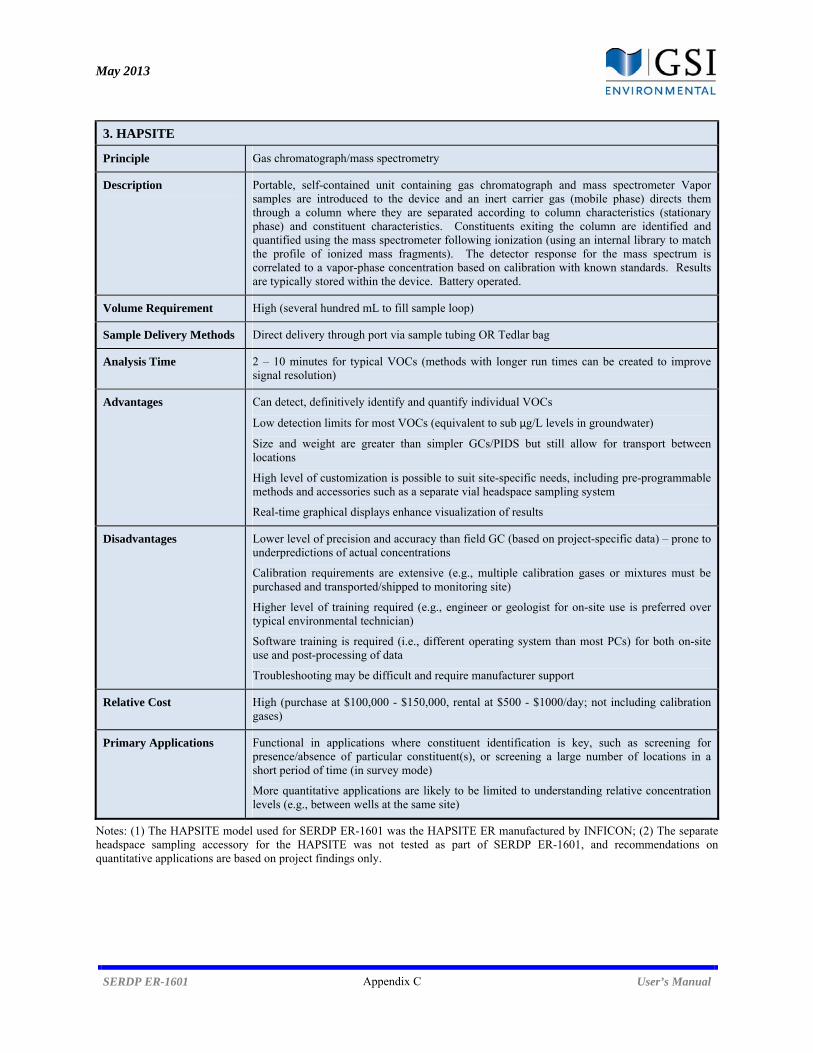
May 2013
SERDP ER-1601 Appendix C User’s Manual
3. HAPSITE
Principle Gas chromatograph/mass spectrometry
Description Portable, self-contained unit containing gas chromatograph and mass spectrometer Vapor samples are introduced to the device and an inert carrier gas (mobile phase) directs them through a column where they are separated according to column characteristics (stationary phase) and constituent characteristics. Constituents exiting the column are identified and quantified using the mass spectrometer following ionization (using an internal library to match the profile of ionized mass fragments). The detector response for the mass spectrum is correlated to a vapor-phase concentration based on calibration with known standards. Results are typically stored within the device. Battery operated.
Volume Requirement High (several hundred mL to fill sample loop)
Sample Delivery Methods Direct delivery through port via sample tubing OR Tedlar bag
Analysis Time 2 – 10 minutes for typical VOCs (methods with longer run times can be created to improve signal resolution)
Advantages Can detect, definitively identify and quantify individual VOCs
Low detection limits for most VOCs (equivalent to sub μg/L levels in groundwater)
Size and weight are greater than simpler GCs/PIDS but still allow for transport between locations
High level of customization is possible to suit site-specific needs, including pre-programmable methods and accessories such as a separate vial headspace sampling system
Real-time graphical displays enhance visualization of results
Disadvantages Lower level of precision and accuracy than field GC (based on project-specific data) – prone to underpredictions of actual concentrations
Calibration requirements are extensive (e.g., multiple calibration gases or mixtures must be purchased and transported/shipped to monitoring site)
Higher level of training required (e.g., engineer or geologist for on-site use is preferred over typical environmental technician)
Software training is required (i.e., different operating system than most PCs) for both on-site use and post-processing of data
Troubleshooting may be difficult and require manufacturer support
Relative Cost High (purchase at $100,000 - $150,000, rental at $500 - $1000/day; not including calibration gases)
Primary Applications Functional in applications where constituent identification is key, such as screening for presence/absence of particular constituent(s), or screening a large number of locations in a short period of time (in survey mode)
More quantitative applications are likely to be limited to understanding relative concentration levels (e.g., between wells at the same site)
Notes: (1) The HAPSITE model used for SERDP ER-1601 was the HAPSITE ER manufactured by INFICON; (2) The separate headspace sampling accessory for the HAPSITE was not tested as part of SERDP ER-1601, and recommendations on quantitative applications are based on project findings only.

May 2013
SERDP ER-1601 Appendix C User’s Manual
A. ppbRAE 3000 PID B. Photovac Voyager GC C. HAPSITE ER
Figure 12. Field-portable instruments used for the on-site analysis of vapor-phase VOCs.
Figure 13. Example of vapor sample transfer using the short PVDs. 100-µL vapor samples from the PVDs were removed with a gas-tight glass micro-syringe for subsequent analyses.
Figure 14. Example of vapor analyses using the field-portable GC. All analyses were conducted immediately after sample was collected.
A B C
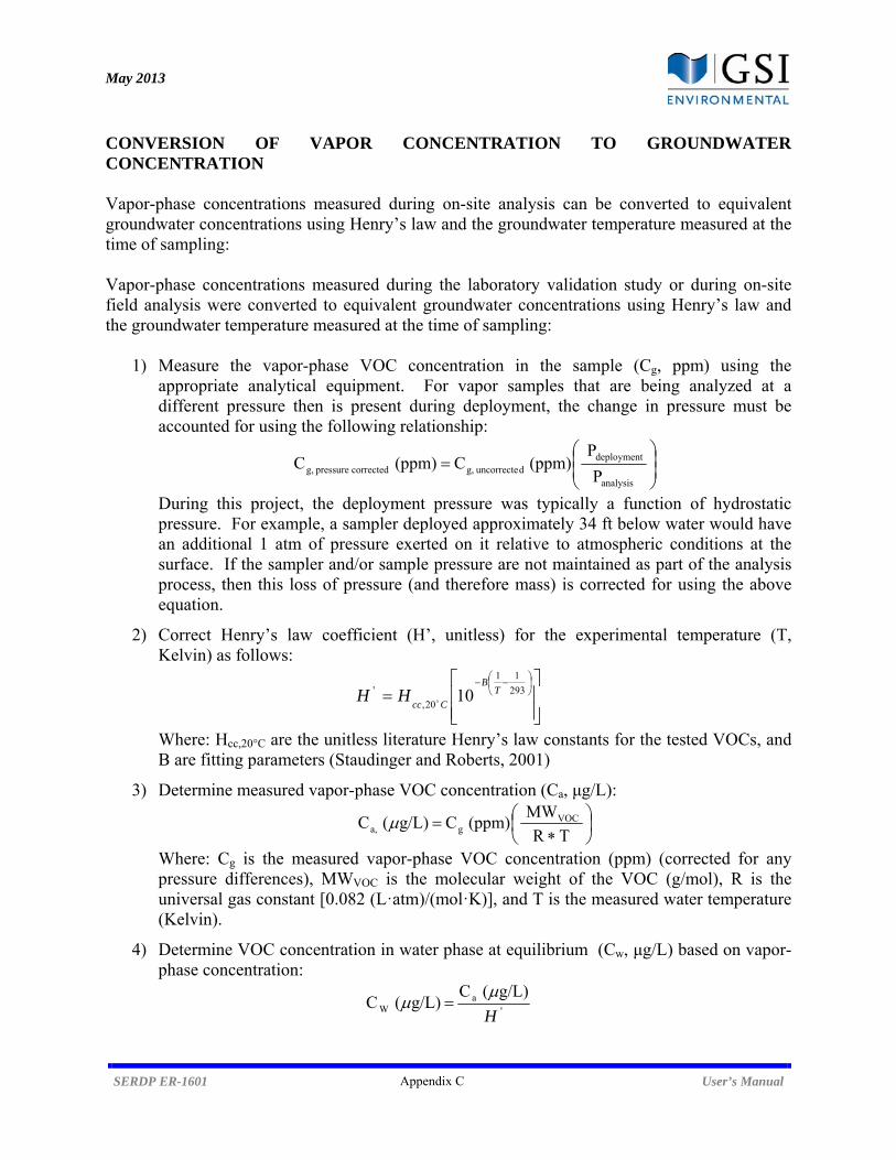
May 2013
SERDP ER-1601 Appendix C User’s Manual
CONVERSION OF VAPOR CONCENTRATION TO GROUNDWATER CONCENTRATION Vapor-phase concentrations measured during on-site analysis can be converted to equivalent groundwater concentrations using Henry’s law and the groundwater temperature measured at the time of sampling: Vapor-phase concentrations measured during the laboratory validation study or during on-site field analysis were converted to equivalent groundwater concentrations using Henry’s law and the groundwater temperature measured at the time of sampling:
1) Measure the vapor-phase VOC concentration in the sample (Cg, ppm) using the appropriate analytical equipment. For vapor samples that are being analyzed at a different pressure then is present during deployment, the change in pressure must be accounted for using the following relationship:
analysis
deploymentduncorrecte g,corrected pressure g, P
P(ppm) C (ppm) C
During this project, the deployment pressure was typically a function of hydrostatic pressure. For example, a sampler deployed approximately 34 ft below water would have an additional 1 atm of pressure exerted on it relative to atmospheric conditions at the surface. If the sampler and/or sample pressure are not maintained as part of the analysis process, then this loss of pressure (and therefore mass) is corrected for using the above equation.
2) Correct Henry’s law coefficient (H’, unitless) for the experimental temperature (T, Kelvin) as follows:
293
11
20,
' 10 TB
CccHH
Where: Hcc,20°C are the unitless literature Henry’s law constants for the tested VOCs, and B are fitting parameters (Staudinger and Roberts, 2001)
3) Determine measured vapor-phase VOC concentration (Ca, μg/L):
TR
MW(ppm) C g/L)( C VOC
ga,
Where: Cg is the measured vapor-phase VOC concentration (ppm) (corrected for any pressure differences), MWVOC is the molecular weight of the VOC (g/mol), R is the universal gas constant [0.082 (L·atm)/(mol·K)], and T is the measured water temperature (Kelvin).
4) Determine VOC concentration in water phase at equilibrium (Cw, μg/L) based on vapor-phase concentration:
'a
W
g/L)( C g/L)( C
H
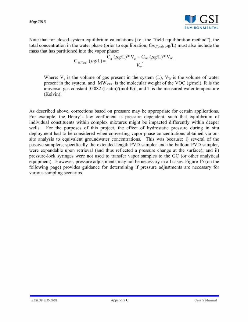
May 2013
SERDP ER-1601 Appendix C User’s Manual
Note that for closed-system equilibrium calculations (i.e., the “field equilibration method”), the total concentration in the water phase (prior to equilibration; CW,Total, μg/L) must also include the mass that has partitioned into the vapor phase:
'
WWaTotalW,
V*g/L)( CV*g/L)( C g/L)( C
W
g
V
Where: Vg is the volume of gas present in the system (L), VW is the volume of water present in the system, and MWVOC is the molecular weight of the VOC (g/mol), R is the universal gas constant [0.082 (L·atm)/(mol·K)], and T is the measured water temperature (Kelvin).
As described above, corrections based on pressure may be appropriate for certain applications. For example, the Henry’s law coefficient is pressure dependent, such that equilibrium of individual constituents within complex mixtures might be impacted differently within deeper wells. For the purposes of this project, the effect of hydrostatic pressure during in situ deployment had to be considered when converting vapor-phase concentrations obtained via on-site analysis to equivalent groundwater concentrations. This was because: i) several of the passive samplers, specifically the extended-length PVD sampler and the balloon PVD sampler, were expandable upon retrieval (and thus reflected a pressure change at the surface); and ii) pressure-lock syringes were not used to transfer vapor samples to the GC (or other analytical equipment). However, pressure adjustments may not be necessary in all cases. Figure 15 (on the following page) provides guidance for determining if pressure adjustments are necessary for various sampling scenarios.
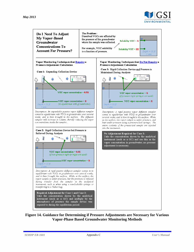
May 2013
SERDP ER-1601 Appendix C User’s Manual
Figure 14. Guidance for Determining if Pressure Adjustments are Necessary for Various Vapor-Phase Based Groundwater Monitoring Methods
Related Documents