Final Project Monte Carlo Markov Chain Simulation To Calculate Elevator’s Round Trip Time under incoming traffic conditions UNIVERSITY OF JORDAN Faculty of Engineering and Technology Mechatronics Engineering Department January, 2013 Supervisor Dr. Lutfi Rawhi Al-sharif By Hasan Shaban Algzawi Submitted as a report in the partial fulfillment for the award of degree of B.Sc. in Mechatronics

Welcome message from author
This document is posted to help you gain knowledge. Please leave a comment to let me know what you think about it! Share it to your friends and learn new things together.
Transcript
Final Project
Monte Carlo Markov Chain Simulation To Calculate Elevator’s Round Trip Time under incoming
traffic conditions
UNIVERSITY OF JORDAN Faculty of Engineering and Technology Mechatronics Engineering Department
January, 2013
Supervisor Dr. Lutfi Rawhi Al-sharif
By Hasan Shaban Algzawi
Submitted as a report in the partial fulfillment for the award of degree of B.Sc. in Mechatronics

DISCLAIMER This report was written by student(s) at the Mechatronics Engineering Department,
Faculty of Engineering and Technology, The University of Jordan. It has not been altered or corrected (other than editorial corrections) as a result of
assessment and it may contain errors. The views expressed in it together with any recommendations are those of the student(s). The University of Jordan
accepts no responsibility or liability for the consequences of this report being used for a purpose other than the purpose for which it was commissioned.

Certificate
Certifies that the work contained in this report entitled:
Was carried out by
Hasan Shaban Algzawi
Under my supervision and that in my opinion, it is fully adequate, in scope and quality, for the requirements of the graduation project in Mechatronics Engineering Department.
Supervisor
Dr. Lutfi Rawhi Al-sharif
Mechatronics Engineering Department
Faculty of Engineering and Technology
University of Jordan, Amman, Jordan

Acknowledgements
I would like to thank Dr. Lutfi Al-Sharif whose encouragement, guidance and support from the
initial to the final level helped me a lot in the accomplishment of this project.
And special thanks to Eng. Ahmed Taiseer who has made available his support in a number of
ways.
Hasan Al-Gzawi

i
TABLE OF CONTENTS
Page
Table of Contents……………………………………………………………………i List of figures…………………………………………………..................................iv List of Tables………………………………………………......................................viiNomenclature………………………………………………......................................viiiiAbstract………………………………………………………………………………x Dedication……………………………………………………………………...…….xi
Chapter 1: Introduction to the design of elevator systems…………………….......1
1.1 History of elevators………………………………………..………………………2 1.2 Elevator Traffic Analysis………………...…………………………….….............3
1.2.1 Elevator traffic analysis definition………………………………..………..31.2.2 Round trip time……………………………………………….……............4
1.2.2.1 Definition of Round trip time……………………............................41.2.2.1 Importance and uses of Round trip time…………………….……...5
Chapter 2: Introduction to Monte Carlo Markov Chain.……………………..….7
2.1 Markov Chains…………………………………………….………………………8
2.1.1 Markov Chain Formal definition…………………………………….…….9 2.1.2 Example of a Markov chain……………………………………………….102.1.3 Applications of Markov Chains……………………………………..…….11
2.2 Monte Carlo Markov Chains…………………………………………...................112.2.1 Applications of Monte Carlo Markov Chains………………………..........12
Chapter 3: Monte Carlo Markov Chain and Monte Carlo simulation methods to calculate Round trip time……………………………………………………...……...13 3.1 Introduction.………………………………………………………………………14

ii
3.2 Monte Carlo Markov Chain simulation method……………………………….14 3.2.1 The transition probability matrix…………………………………..…...14
3.2.1.1 The probability of elevator’s transition between any two floors……………………………………….............................................143.2.1.2 The probability of elevator’s transition from the main floor to any other floor…………………………………………………………...…..19
3.2.2 Random Scenario Generation…………………………………………..213.2.3 Calculation of the kinematics time…………………………………..…22 3.2.4 Calculation of the constant time………………..………………….…...24 3.2.5 Calculation of the round trip time………………………………….…..253.2.6 Trials of the procedure…………………………………………………25
3.3 Monte Carlo Simulation method………………………………………………25 3.3.1 Drawing the PDF and CDF graphs of the floor population percentage…………………….……………………………………………...26 3.3.2 Generation of the random journey scenario…………...........................27 3.3.3 Calculation of the round trip time…………………………………......27
3.3.4 Trials of the procedure………………………………………………...27 3.4 The analytical solution………………………………………………………..28 Chapter 4: Software Simulation………………………………….……………31
4.1 Introduction………………………………………………………………….324.2 The MATLAB GUI round trip time simulation tool…………………….….32 Chapter 5: Results, Conclusions and recommendations…..............................36 5.1 Case study 1…………………………………………………………………37 5.2 Case study 2…………………………………………………………………47 5.3 Conclusions and future work……………………………………..................60
References……………………………………………………………………....61 Appendix: MATLAB GUI Code for the software tool……………….........62

iii
LIST OF FIGURES
page
Figure 1.1: Elevator’s shaft…………………………………………………….…...2
Figure 1.2: An old and a new kind of elevators…………………………………….2
Figure 1.3: Waiting time…………………………………………………………....3
Figure 1.4: the round trip time timeline during up-peak traffic……………………..5
Figure 2.1. Markov Chain………………………………………………………......8
Figure 2.2. Markov chain for music notes………………………………………...10
Figure 3.1: PDF graph for the current floor i……………………………………...22
Figure 3.2: CDF graph for the current floor i………………………………….......22
Figure 3.3: Transition time and constant time…………………………………......23
Figure 3.4: PDF graph for the current floor i…………………………………...…27
Figure 3.5: CDF graph for the current floor i…………………………………..….27
Figure 4.1: The MATLAB GUI round trip time simulation tool……………….....32
Figure 4.2: Block diagram of the Monte Carlo Markov Chain round trip time
tool………………………………………………………………………………....34
Figure 4.3: Block diagram of the Monte Carlo round trip time simulation
tool……………………………………………………………………………..…..35
Figure 5.1: the probability density function of the floors population
percentage……………………………………………………………………….....38
Figure 5.2: The cumulative density function of the floors population
percentage……………………………………………………………………….....39
Figure 5.3: PDF of the ground floor…………………………………………….....41
Figure 5.4: CDF of the ground floor……………………………………………….41
Figure 5.5: PDF of the first floor…………………………………………….….....41
iv
Figure 5.6: CDF of the first floor………………………………………………......41
Figure 5.7: PDF of the second floor……………………………………………......42
Figure 5.8: CDF of the second floor…………………………………………….....42
Figure 5.9: PDF of the third floor…………………………………………….........42
Figure 5.10: CDF of the third floor…………………………………………….......42
Figure 5.11: PDF of the fourth floor……………………………………………….43
Figure 5.12: CDF of the fourth floor……………………………………………....43
Figure 5.13: PDF of the fifth floor………………………………………………...43
Figure 5.14: CDF of the fifth floor………………………………………………...43
Figure 5.15 : Percentage of error versus number of trials in log scale…….............46
Figure 5.16: The probability density function of the floors population
percentage……………………………………………………………………….….48
Figure 5.17: The Cumulative density function of the floors population
percentage…………………………………………………………………….…….49
Figure 5.18: PDF of the ground floor………………………………………………51
Figure 5.19: CDF of the ground floor……………………………………………...51
Figure 5.20: PDF of the first floor…………………………………………………52
Figure 5.21: CDF of the first floor………………………………………………....52
Figure 5.22: PDF of the second floor……………………………………………....52
Figure 5.23: CDF of the second floor……………………………………………...52
Figure 5.24: PDF of the third floor………………………………………………...53
Figure 5.25: CDF of the third floor………………………………………………...53
Figure 5.26: PDF of the fourth floor…………………………………………….....53
Figure 5.27: CDF of the fourth floor……………………………………………....53
Figure 5.28: PDF of the fifth floor…………………………………………….......54
Figure 5.29: CDF of the fifth floor…………………………………………….......54

v
Figure 5.30: PDF of the sixth floor…………………………………………….....54
Figure 5.31: CDF of the sixth floor…………………………………………….....54
Figure 5.32: PDF of the seventh floor…………………………………………….55
Figure 5.33: CDF of the seventh floor…………………………………………….55
Figure 5.34: PDF of the eighth floor……………………………………………...55
Figure 5.35: CDF of the eighth floor……………………………………………...55
Figure 5.36: PDF of the ninth floor..……………………………………………...56
Figure 5.37: CDF of the ninth floor………………………………………………56
Figure 5.38: PDF of the tenth floor……………………………………………….56
Figure 5.39: CDF of the tenth floor………………………………………………56
Figure 5.40 : Percentage of error versus number of trials in log scale…………....59

vi
LIST OF TABLES
page
Table2.1: transition probability matrix for the music notes A, C, E……….........10
Table 3.1: The elevator’s Transition probability matrix , G: ground floor, N:
highest floor……………………………………………………………..………20
Table 3.2: Normalization of the floor population, where U is the total
population……………………………………………………………….…….…26
Table5.1: the transition probability matrix of case study 1………….………….40
Table 5.2: the simulation software results for the values of round trip time using
MCMC and MC methods for different number of trials for case study 1…….....45
Table 5.3: percentage of error for Monte Carlo Markov chain method and Monte
Carlo method for case study 1…………………………………………………...46
Table 5.4: the transition probability matrix for case study 2……………..…….51
Table 5.5: the simulation software results for the values of round trip time using
MCMC and MC methods for different number of trials for case study 2……….58
Table 5.6: percentage of error for Monte Carlo Markov chain method and Monte
Carlo method for case study 2……………………………………………….…..59

vii
LIST OF NOMENCLATURE
RTT: Round Trip Time.
MCMC: Monte Carlo Markov Chain.
MC: Monte Carlo.
PDF: Probability Density Function.
CDF: cumulative Distribution function.
HC: Handling Capacity.
Int.: Interval.
CC: Car Capacity.
GUI: Graphical User Interface.
s: Seconds.
: round trip time.
L: number of elevators.
N: the total number of floors.
U: population of the building.
Ui : The ith floor population.
P: number of passengers inside the elevator.
S: Probable number of stops.
H: Highest reversal floor.
Pr: Probability.
Pij : The probability of going from state i to state j in n time steps.
J: journey. ijJP : The probability of the elevator’s making a journey between floor i and floor j
iSP : The probability of the elevator’s stopping at floor i

viii
d: distance traveled [ m]
: The rated speed [m/s] a: Acceleration [m/s2 ] j: Jerk [m/s3 ]
: Kinematics time [s].
: Time needed for the elevator’s transition between two floors [s] df: finished floor to finished floor level [m]
: Door opening time. [s]
: Door closing time. [s]
: Passenger’s boarding time. [s]
: Passenger’s alighting time. [s]
: theroundtriptimefoundinthei trial [s]
: The time spent at the ground floor [s]
: The time spent travelling to the upper destination floors and delivering the passengers [s]
: The time spent returning back to the ground terminal from the highest reversal floor [s] tsd: Motor start delay [s] tao: Advance door opening time [s] tacc : the time taken to accelerate up to the top speed from standstill [s] tdec : the time taken to decelerate down from the top speed down to standstill [s] e%: percentage of error.
ix
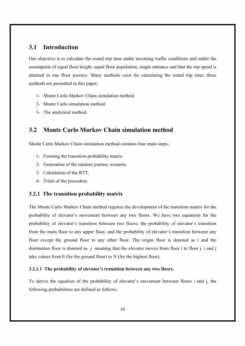
Abstract
Nowadays the challenge of the development of elevator systems involves the improvement of the
quality and quantity of service to provide the passengers the minimum waiting or travelling time,
or to reduce the consumption of power in a group of elevators system through elevator traffic
analysis. The design of elevator system is based on determining the number, speed and capacity
of elevators. Elevator traffic analysis depends mainly on the calculation of the Round trip time,
therefore in this report a Monte Carlo Markov Chain simulation method is introduced to
calculate the round trip time under incoming (up-peak) traffic conditions and with the
assumptions of equal number of floor population, equal floor heights and a top speed that is
attained in a one floor journey.
Monte Carlo Markov Chain simulation method is a numerical probabilistic method based on a
large number of trials to approach the exact value. The availability of powerful computing
programs that are easily accessed by computers and laptops, that is spread everywhere and exist
almost in every house, made it practical and easy to use the Monte Carlo Markov Chains
simulation in evaluating the round trip time value of elevator systems, where it is easy to run tens
of thousands of simulation runs within fractions of a second.
Another simulation method; Monte Carlo Simulation method, is also presented in this report,
where the results of this method is compared to the Monte Carlo Markov chains simulation
method. Results of the simulation show that the Monte Carlo Markov Chains method is better
than the Monte Carlo method where the Monte Carlo Markov chains method gives very accurate
value and with easiness of software simulation and a less number of trials compared to the
number of trials required for satisfactory result using the Monte Carlo Simulation method.
The power of the Monte Carlo Markov Chains simulation method is that it is easy to develop it
for calculating the round trip time if either one or more of the assumptions of equal floor heights,
equal floor population and that the top speed is attained in a one floor journey were dropped.

1
Chapter One
Introduction to the design of elevator systems

2
1.1 History of elevators
The elevator is a lifting device that is moved vertically to transport people or things up or down
along a vertical shaft. The shaft is usually made of cables, motor and the operating equipments.
See figure 1.1.
Figure 1.1: Elevator’s shaft
Elevators were developed through history from a simple lift powered by animals, water wheels
power or even by hand to a lift powered by hoist and afterwards powered by a steam. Then the
development of elevators continued to after that becomes powered by electricity. The
development of industries and the need for transporting of materials in factories was mainly the
reason of developing of elevators systems.[1]. Also, the production of Electrical elevators
revolutionized the use of elevators in industries and buildings up to this level that we have today,
see figure 1.2.
Figure 1.2: An old and a new kind of elevators

3
1.2 Elevator Traffic Analysis
1.2.1 Elevator traffic analysis definition
Elevator traffic analysis is studying and analyzing the performance of a group of elevators based
on assumptions about the expected traffic situation.
The objective of elevator traffic analysis is to find the suitable elevators that satisfy the
performance desired for a building; number, velocity and capacitance of elevators will be
determined.
The main performance measurements are quantity of service and quality of service, where the
quantity of service refers to the handling capacity and the quality of service refers to the interval.
Handling Capacity is the percentage of the building population that the group of elevators
can support in a given time period (usually in 5 minutes).
Interval is the average time between the arriving of tow elevators, and it can be a good
measure of the waiting time of the passengers at the main floor. see figure.1.3.
Figure 1.3: Waiting time
The elevator traffic analysis is based on assumptions about the movement of the building
population, for example when and where do they enter or leave and are there facilities like
restaurants, gyms…etc in the building that affects the usual passengers flowing in and out.
If the assumptions of population movement in the building were accurate, then the results of the
traffic analysis will be accurate too, because then we can make an accurate calculation of the
elevator performance.
The outputs of a traffic analysis will give an accurate indication of the quality and quantity of the
elevator service provided, like the calculation of waiting times and the percentage of the building
population that can be transported by the elevators in a given period of time.

4
Elevator traffic analysis is used in the design of new buildings or existing buildings. In new
buildings it is used in the design of elevators to know the size, speed and capacity of elevators
needed to provide the quantity and quality levels of service required.
For existing buildings elevator traffic analysis are used to predict the effect of changes in a
building’s population or configuration on the elevator service, because the population of building
is often increased and sometimes some features are added to it or changed like restaurants,
gyms…etc. These changes can affect the flow of people [2].
There are four main types of elevator traffic modes;
1- Up peak traffic.
2- Down peak traffic.
3- Lunch time (two way) traffic.
4- Inter-floor traffic.
In this research, we will focus on the incoming (up-peak) traffic, which states that the passengers
arrives at the main terminal and then being transported to the upper floors, then the elevator
returns to the terminal floor to pick up passengers again to the upper floors.
1.2.2 Round trip time
1.2.2.1 Definition of Round trip time
The round trip time (RTT) is the time needed for a single elevator to complete a closed path in a
building, or the time needed for the passengers to travel from the main floor (ground floor) to the
highest reversal floor and back to the main floor.
The round trip time starts from the door opening at main floor and ends with door opening, see
figure 1.4. The highest reversal floor is the highest floor that the elevator reaches in one journey.
The round trip time is the most important parameter in the design of modern elevator systems
and in elevator traffic analysis. Modern buildings are becoming more complicated and more
sophisticated. Therefore, it is an important task to develop accurate methods for the calculation
of the round trip time that catches up with the development of the modern buildings.

5
Figure 1.4: the round trip time timeline during up-peak traffic
It is clear from the graph that the round trip time in the up peak traffic contains four components;
the time needed to collect passengers at the main floor, the time needed to deliver passengers to
their destinations, the time spent in stopping at each destination floor and the time spent by the
elevator while returning to the main floor.
1.2.2.1 Importance and uses of Round trip time
The RTT is important because it is used to indicate the elevator’s performance, because it is
related to the handling capacity as shown in the following equation.
U
PLHC
300%
(1.1 )[10]
Where :
HC%: handling capacity.
L : number of elevators.
P: number of passengers inside the elevator.
: round trip time.
U: population of the building.
RTT

6
Also the round trip time is used to measure the interval [3], because the interval is calculated by
dividing the round trip time by the number of elevators , see the following equation.
(1.2)[10]
Where:
L : number of elevators.
: round trip time.
Usually the performance of elevator system is determined in the incoming traffic situation, where
passengers move from the ground floor to upper floors. That is because the incoming traffic is a
difficult traffic situation. There are many methods for calculating the RTT in the incoming traffic
situation. The simplest method is based on calculating the expected number of stops and the
expected highest reversal floor and substituting them in the RTT equation [3].
For more accurate result we should not just calculate the number of stops, but also we should
calculate the probability of flow between each pair of floors for incoming traffic. Hence we will
introduce another two methods for calculating round trip time which are the Markov Chain
method and Monte Carlo Markov Chain method. Before discussing these three methods
mentioned above we will give a brief description of the meaning of Markov chains and Monte
Carlo Markov Chains.

7
Chapter two
Introduction to Monte Carlo Markov Chain

8
2.1 Markov Chains
A Markov chain, is a mathematical system that undergoes transitions from one state to another,
see figure 2.1. The number of possible states is finite or countable. Markov chain is a random
process usually described as memoryless; meaning that the next state depends only on the current
state and does not depend on the sequence of events after it. This "memorylessness" is called the
Markov property. Therefore, a Markov chain can be described as a random process with the
Markov property. Markov chains are very useful and have many applications as statistical
models of real-world processes.
Figure 2.1: Markov Chain
Often, the term "Markov chain" is used to mean a Markov process which has a discrete state-
space, meaning that the number of states is finite or countable. Usually a Markov chain is
defined for a discrete set of times ( it is expressed as “ a discrete-time Markov chain” )[4]
although some authors use the same expression where "time" can take continuous values.[5,6] The
use of the term in Markov chain Monte Carlo method covers cases where the process is in
discrete time (discrete algorithm steps) with a continuous state space.
A discrete-time random process is a system which is in a certain state at each step, by going from
one discrete step to another the state changes. The steps are often moments in time, but they can
also refer to physical distance or any other discrete measurement; in other words, the steps are
the integers, and the random process is a mapping of these steps to states. The Markov property
means that the probability for the system at the next step depends only on the current state of the
system, and not on the state of the system at previous steps.

9
The changes of states of the system are called ‘transitions’, and the probabilities of the various
state-changes are called ‘transition probabilities’. The set of all states and transition probabilities
completely makes a Markov chain. By convention, we assume all possible states and transitions
have been included in the definition of the processes, so there is always a next state and the
process goes on forever.
The system changes randomly, therefore it is impossible to predict with certainty the state of a
Markov chain at a given point in the future. But the statistical properties of the system's future
can be predicted. It is these statistical properties that are important.
2.1.1 Markov Chain Formal definition
A Markov chain is a sequence of random variables X1, X2, X3, ... with the Markov property, such
that, given the present state, the future and past states are independent. Formally,
(2.1)
Where:
Pr: Probability.
The possible values of Xi form a countable set S called the state space of the chain. Markov
chains are often described by a directed graph, where the edges are labeled by the probabilities of
going from one state to the other states as seen before in figure 2.1. The probability of going
from state i to state j in n time steps is
(2.2)
Note: The superscript (n) is an index and not an exponent.
Where:
Pij : is the probability of going from state i to state j in n time steps.
The single-step transition is
(2.3)

10
2.1.2 Example of a Markov chain
Markov chains are used in music composition or making a song melody. The states of the system
are the note values and there’s a probability vector for each note, see figure2.2. Completing a
transition probability matrix, see Table 2.1. An algorithm is constructed to produce an output
note values based on the transition matrix probabilities. [7]
Figure 2.2: Markov chain for music notes
Table2.1: transition probability matrix for the music notes A, C, E

11
2.1.3 Applications of Markov Chains
Markov chains are applied to many different fields, some of them are:
Physics
Medicine
Information sciences
Queueing theory
Internet applications
Social sciences
Chemistry
Games
Music
Statistics
2.2 Monte Carlo Markov Chains
Markov chain Monte Carlo (MCMC) methods are a class of algorithms for sampling using
probability distributions. It is based on constructing a Markov chain that has the desired
distribution as its stationary distribution. The state of the chain after a large number of steps is
then used as a sample of the desired distribution. As the number of steps increases, the quality of
the sample improves.
It is not hard to construct a Markov chain with the desired properties. The difficult thing is to
determine how many steps are needed to get close to the stationary distribution with a small
error. A good chain will reach the stationary distribution quickly starting from any position.

12
2.2.1 Applications of Monte Carlo Markov Chains
MCMC methods are useful for simulating events with uncertainty in inputs and systems with a
large number of coupled degrees of freedom. Fields of application include:
Physical sciences
Engineering
Computational biology
Games
Design and visuals
Finance and business
Telecommunications
Applied statistics
In this paper the application of Markov chain methods used is statistics, because we will use
Markov chain Monte Carlo method to generate a sequence of random numbers to reflect the
probability distribution that is desired.

13
Chapter three
Monte Carlo Markov Chain and Monte Carlo simulation methods to calculate Round trip time
14
3.1 Introduction
Our objective is to calculate the round trip time under incoming traffic conditions and under the
assumption of equal floor height, equal floor population, single entrance and that the top speed is
attained in one floor journey. Many methods exist for calculating the round trip time; three
methods are presented in this paper;
1- Monte Carlo Markov Chain simulation method.
2- Monte Carlo simulation method.
3- The analytical method.
3.2 Monte Carlo Markov Chain simulation method
Monte Carlo Markov Chain simulation method contains four main steps;
1- Forming the transition probability matrix.
2- Generation of the random journey scenario.
3- Calculation of the RTT.
4- Trials of the procedure.
3.2.1 The transition probability matrix
The Monte Carlo Markov Chain method requires the development of the transition matrix for the
probability of elevator’s movement between any two floors. We have two equations for the
probability of elevator’s transition between two floors; the probability of elevator’s transition
from the main floor to any upper floor, and the probability of elevator’s transition between any
floor except the ground floor to any other floor. The origin floor is denoted as i and the
destination floor is denoted as j. meaning that the elevator moves from floor i to floor j. i and j
take values from 0 (for the ground floor) to N (for the highest floor).
3.2.1.1 The probability of elevator’s transition between any two floors.
To derive the equation of the probability of elevator’s movement between floors i and j, the
following probabilities are defined as follows.

15
ijJP is the probability of the elevator making a journey between floor i and floor j without
stopping at any of the floors in between.
iSP is the probability of the elevator stopping at floor i.
jSP is the probability of the elevator stopping at floor j.
1,2,...,2,1 jjiiSP is the probability of the elevator stopping at any of the floors between floors
i and j.
iSP is the probability of the elevator not stopping at floor i.
jSP is the probability of the elevator not stopping at floor j.
1,2,...,2,1 jjiiSP is the probability of the elevator not stopping at any of the floors between
floors i and j.
In order for an elevator to make a journey from floor i to floor j without stopping at any of the
middle floors in between, the following statement should be true:
The elevator stops at i
AND
The elevator stops at j
AND
The elevator does not stop at any of the in between floors (i+1, i+2, i+3….j-2, j-1)
This statement could be expressed mathematically as follows:
1,2....2,1 jjiijiij SPSPSPJP
(3.1) [8]
This could be rewritten as:
1,2....2,111 jjiijiij SPSPSPJP
(3.2) [8]
16
Expanding gives:
jijijjiiij SPSPSPSPSPJP 11,2....2,1 (3.3) [8]
jjjiii
jjjiijjiiijjiiij
SPSPSP
SPSPSPSPSPJP
1,2....2,1
1,2....2,11,2....2,11,2....2,1
(3.4) [8]
But:
1,2....2,1,1,2....2,1 jjiiijjiii SPSPSP
(3.5) [8]
And:
jjjiijjjii SPSPSP ,1,2....2,11,2....2,1
(3.6) [8]
And:
jjjiiijjjiii SPSPSPSP ,1,2....2,1,1,2....2,1
(3.7) [8]
Substituting (3.5), (3.6) and (3.7) in (3.4) gives the following result:
jjjiiijjjiijjiiijjiiij SPSPSPSPJP ,1,2....2,1,,1,2....2,11,2....2,1,1,2....2,1
(3.8) [8]
For the case of incoming traffic only and a single entrance, the probability of not stopping at a
number of floors can be derived as follows:
1,2.....2,1,1,21,1,2....2,1, /.....// jjiiijiiiiiijjjiii SSPSSPSSPSPSP
(3.9) [8]
Where the expression 1,2 / iii SSP
represents a conditional probability that stands for the
probability that a stop will not take place on floor i+2 given that no stops have taken place on
floors i and i+1.

17
Developing equation (3.9) further gives:
P
jii
j
P
ii
i
P
i
i
P
ijjjiii
UUUU
U
UUU
U
UU
U
U
USP
11
1
21,1,2....2,1,
........1........
.....111
(3.10) [8]
Where:
U: total building population.
Ui : ith floor population.
Developing equation (3.10) further gives:
P
jii
jjii
P
ii
iii
P
i
ii
P
ijjjiii
UUUU
UUUUU
UUU
UUUU
UU
UUU
U
UUSP
11
11
1
211,1,2....2,1,
........
................
.
(3.11) [8]
P
jii
jjii
ii
iii
i
iii
jjjiii
UUUU
UUUUU
UUU
UUUU
UU
UUU
U
UU
SP
11
11
1
211
,1,2....2,1,
........
................
.....
(3.12) [8]
P
jii
jjii
ii
iii
i
iii
jjjiii
UUUU
UUUUU
UUU
UUUU
UU
UUU
U
UU
SP
11
11
1
211
,1,2....2,1,
........
................
.....
(3.13) [8]

18
P
jjii
P
jjiijjjiii
U
UUUU
U
UUUUUSP
11
11,1,2....2,1,
........1
........
(3.14) [8]
This leads to the general formula:
Pj
ik
kjjjiii U
USP
1,1,2....2,1,
(3.15) [8]
Substituting (3.15) in (3.8) gives equation (3.16) which performs the probabilities of elevator
transitions between floor i and floor j when the current floor i is the ground floor (i=0):
Pj
ik
k
Pj
ik
k
Pj
ik
k
Pj
ik
kij U
U
U
U
U
U
U
UJP
11111
11
1 (3.16) [8]
But the probability that the elevator is stopping at floor i is:
1 1 (3.17) [8]
By dividing equation (3.16) by equation (3.17), we get equation (3.18) which performs the
probabilities of elevator transition from floor i to floor j when the elevator is stopping at floor i :
(3.18) [8]
Where:
i: current state (floor).
j: next state (floor).
P: number of passengers.
: each floor population.
U: total population.
J: journey.
19
3.2.1.2 The probability of elevator’s transition from the main floor to any other floor
For the special case where the journey’s origin is the ground floor, the probability of a journey
between the ground floor (floor 0) and floor j, can be developed as follows using equation (3.1)
and substituting 0 for the value of i:
1,2....3,2,100 jjjj SPSPSPJP
(3.19) [8]
But here the probability of stopping at the ground floor is 1 as the ground floor is the only
entrance and the elevator must stop at this floor in every journey to pick up the passengers. So
the equation above becomes:
1,2....3,2,11,2....3,2,10 1 jjjjjjj SPSPSPSPJP
(3.20) [8]
jjjjj SPSPJP ,1....3,2,11,2....3,2,10 (3.21) [8]
Substituting (3.15) in (3.21) gives:
Pj
k
k
Pj
k
kj U
U
U
UJP
1
1
10 11
(3.22) [8]
As long as the elevator is stopping at the ground floor and the elevator transition from the ground
floor to floor j is to be found, then:
1 1 1 (3.23) [8]
By dividing equation (3.22) by equation (3.23) we get the probabilities of elevator transitions
between the ground floor and floor j when the elevator is already stopping at the ground floor:
1111
1
10
Pj
k
k
Pj
k
kj U
U
U
UJP
(3.24)
[8]
By inserting the results obtained from equation (3.18) and equation (3.24) into a matrix, we have
the transition matrix that represents the probabilities of elevator’s transitions between any two
floors; the transition matrix is shown in Table 3.1.

20
Table 3.1: The elevator’s Transition probability matrix , G: ground floor, N: highest floor.
G
1
2
…
…
N-1
N
G
0
…
…
…
1
0
…
…
…
2
0
0
…
…
.
.
.
.
.
0
0
0
…
.
.
.
.
.
.
0
0
0
0
N-1
.
.
.
0
0
0
0
0
N
1
0
0
0
0
0
0
In the transition matrix, the rows represent the current states and the columns represent the future
states. One of the conditions of using Monte Carlo Markov Chain simulation is that the transition
matrix should be a square matrix and as seen from the transition matrix, that condition is
obtained where the transition matrix is an (( 1 1 ) matrix, where N+1 is the total
number of floors of the building. Also the Markov Chain theory states that the summation of
every row in the matrix should equal unity.
As expected the diagonal values are all zeros because the elevator’s probability of transition from
a floor to the same floor is zero as the elevator cannot move to any floor that it is already on
[( 0]. As indicated from the incoming traffic the elevator transfers passengers only in the
upper direction and while it moves down it only stops at the ground floor therefore the lower
triangle values in the transition matrix are all zeros except the first row. For example the

21
probability of elevator’s movement from the second floor to the first floor equals zero [
0]. While the values of the first row of the lower triangle are not zeros because this row
represents the probability of the elevator returning from its position to the ground floor.
Furthermore, the probability of the elevator’s returning from the last floor (N) to the ground floor
equals unity always, it is because at this position the elevator has no other options to move to
except the ground floor.
3.2.2 Random Scenario Generation
After deriving the probability equations and arranging them in the transition matrix we can
generate random scenarios for the elevator’s transition depending on the probability function.
The random scenario is the elevator’s journey from the ground floor up to the destination floors
and returning to the ground floor. The selection process of the destination floors depends on the
transition matrix.
Therefore we shall sketch the Probability Density Function (PDF) and the Cumulative
Distribution Function (CDF) for every current floor recalling that rows of the transition matrix
corresponds to current floors, i.e. first row corresponds to first floor and second row corresponds
to second floor,…etc.
Probability Density Function (PDF) is a function representing the relative distribution of
frequency of the elevator’s transition between two floors, see figure 3.1.The probability density
function is nonnegative everywhere, and its integral over the entire space is equal to one. PDF
has the property that its integral from a to b is the probability that the variable lies in this interval,
hence we also sketch the cumulative density function. Cumulative Distribution Function (CDF)
is the sum or integral function of the probability density function, see figure 3.2.

22
Figure 3.1: PDF graph for the current floor i.
Figure 3.2: CDF graph for the current floor i
We start the elevator’s journey at the ground floor as the passengers enter the elevator only at the
ground floor and then we take a random value between (0-1) and scan the CDF of the ground
floor to find which interval this number belongs to; hence we determine the destination floor
(future state). In the next step the previous future state floor becomes the current state floor so we
take another random value between (0-1) and scan the CDF of the corresponding current floor
and find the interval that this random value belongs to, to determine the future state floor. We
continue this procedure till we return to the ground floor again; and at the end of this procedure
we will have one random journey scenario.
3.2.3 Calculation of the kinematics time
The kinematics time is the time needed for the elevator to move between floors in the whole
journey; i.e. to move from the ground floor up to the destination floors and then return from the
highest reversal floor to the ground. To calculate the kinematics time we shall calculate the
transition time for each transition between two floors, see figure 3.3.

23
Figure 3.3: Transition time and constant time
The transition time is calculated using one of these equations:
If
aj
jvvad
22
then j
a
a
v
v
dt (3.25)
If
aj
jvvad
j
a2 22
2
3
then 2
j
a
a
d4
j
at
(3.26)
If 2
3
j
a2d then
3
1
j
d32t
(3.27)
Where :
d: distance traveled [ m]
v: velocity [m/s]
a: acceleration [m/s2 ]
j: Jerk [m/s3 ]
Constant time Transition time

24
And because we have assumed that top speed is attained in one floor journey; i.e.
aj
jvvad f
22
, then we use the first formula.
After calculating the transition times from the moment the elevator moves from the ground floor
till it returns to it, the transition times should be summed to give the total kinematics time.
(3.28)
Where:
: Kinematics time.
: Time needed for the elevator’s transition between two floors.
3.2.4 Calculation of the constant time
The constant time represents the time spent by the elevator while it is stopped. It includes the
time needed for the elevator’s door to open and close and the time needed for the passengers to
alight and board. It is calculated using this formula.
(3.29)
Where:
: Door opening time. [s]
: Door closing time. [s]
: Passenger’s boarding time. [s]
: Passenger’s alighting time. [s]
P : number of passengers boarding the car.
S: number of stops in one journey.
Since S is the number of times the elevator stops in each journey, the value of S equals the
number of random numbers we use to complete a whole journey.

25
3.2.5 Calculation of the round trip time
The summation of the kinematics time and the constant time gives the round trip time.
(3.30)
3.2.6 Trials of the procedure
To obtain a RTT value that is very close to the actual value we iterate this procedure for a very
large number of times and find the average of the RTTs found through this formula.
⋯
(3.31)
Where:
: is the number of trials
: theroundtriptimefoundinthe trial
The accuracy of the Monte Carlo Markov chain simulation method depends on the number of
trials. As the number of trials increases, the accuracy of the procedure increases and the round
trip time calculated becomes closer to the exact value which therefore minimizes the percentage
of error.
3.3 Monte Carlo Simulation method
The Monte Carlo method is quite similar to Monte Carlo Markov Chain method where both are
based on the generation of random journey scenarios. In the Monte Carlo Markov chains method
the random scenario generation was based on the transition probability matrix but in the Monte
Carlo method the random scenario generation will be based on both the percentage of floor
population and the number of passengers inside the car[9]. On the other hand, the two methods
differ where in the Monte Carlo Markov Chain method the number of stops was randomly found
and varies from a scenario to another. However, in the Monte Carlo method the number of stops
is constant.

26
The number of passengers is found as the effective capacity of the car based on 80% car-rated
capacity:
CCP 8.0 (3.32) [9]
Where
CC: car capacity.
The Monte Carlo simulation procedure includes four main steps;
1- Drawing the PDF, CDF graphs of the floor population percentage.
2- Generation of the random journey scenario.
3- Calculation of the RTT.
4- Trials of the procedure.
3.3.1 Drawing the PDF and CDF graphs of the floor population percentage
The probability of elevator’s transition between any two floors depends on the population
distribution upon floors. By normalization of each floor population we can calculate the floor
population percentage. Normalization of the floor population is shown in Table 3.2.
Table 3.2: Normalization of the floor population, where U is the total population.
Floor k Floor population Percentage of floor
population
1 u1
2 u2
.
.
.
.
.
.
.
.
.
N-1 uN-1
N uN
Thus, the floor population percentage equals:
…

27
But in our case, we have assumed equal floor population, which means that the floor population
percentage will be equal.
After calculating the population percentage and calculating the number of passengers, PDF and
CDF graphs of the floor population percentage are plotted, see figure3.4 and figure3.5.
Figure 3.4: PDF graph for the current floor i. Figure 3.5: CDF graph for the current floor i
3.3.2 Generation of the random journey scenario
Random numbers are all generated at once, it is necessary to generate (P) number of random
values for each scenario, and then these random numbers is taken and the CDF is being scanned
to find to which interval these numbers belong to, and thus the upper destination floors for all
passengers are generated. Then, as the car becomes empty, the elevator will return to the ground
floor.
3.3.3 Calculation of the round trip time
The procedure of calculating the value of the round trip time is the same as the procedure
previously explained in the Monte Carlo Markov chain simulation method, where the summation
of the kinematics time and constant time gives the round trip time of the random journey
scenario.
3.3.4 Trials of the procedure
After calculating the round trip time of the random journey scenario this procedure must be
repeated for a very large number of times, while the round trip time is found in each time. At the

28
end the average of the round trip times is found to get the round trip time of the system that will
be close to the exact value.
As the number of trials increases, the accuracy of this method increases. But, it is important to
mention that the Monte Carlo simulation method needs more trials to get close to the round trip
time exact value than the trials used in the Monte Carlo Markov chain simulation method.
3.4 The analytical solution
In this method the number of stops, the highest reversal floor and the number of passengers are
found using some equations and are taken as the average number that occurs in one trip journey.
The average number of stops in one trip journey is called the probable number of stops (S). For
equal floor population, the probable number of stops is calculated through this formula:
P
N
111NS (3.33) [10]
Where:
N: the total number of floors.
P:the number of passengers.
The number of passengers (P) is taken as the effective capacity of the car based on 80% car-rated
capacity, which is found in equation (15).
As already mentioned before, the highest reversal floor is the highest floor that the elevator
reaches in one trip journey. For equal floor population the highest reversal floor is found using
this formula:
P1N
1i N
iNH
(3.34) [10]
S, P and H do not need to be integers. These three parameters are then substituted in the RTT
general equation. The round trip time is made up of three main components; the time spent at the
ground floor collecting the passengers, the time needed for the elevator to travel to the upper

29
floors and deliver the passengers to their destinations, and the time needed for the elevator to
return from the highest reversal floor to the ground floor, this is expressed in equation (3.35).
HSG (3.35) [10]
Where:
: The time spent at the ground floor.
: The time spent travelling to the upper destination floors and delivering the passengers.
: The time spent returning back to the ground terminal from the highest reversal floor.
The time spent at the ground floor consists of the door opening time, the time needed for the
passengers to enter the elevator, the door closing time and the motor starting delay minus the
advanced door opening time, Therefore:
piaosddcdoG tPtttt (3.36) [10]
Where:
tdo : Door opening time
tdc: Door closing time
tsd:Motor start delay
tao: Advance door opening time
tpi: Passenger boarding time
P: number of passengers
The time spent delivering the passengers to their destinations consist of two parts; the kinematics
time and constant time. The kinematics time contains the time of transition from the ground floor
to the highest reversal floor, while the constant time is the time caused by all the stops of the
elevator. Each stop causes the elevator to decelerate, open its door, alight passengers, close its
door and then accelerates again, therefore we have this formula:
poaosddcdof
decaccS tPttttSv
dHttS
(3.37) [10]
Where:
S: probable number of stops.

30
H: highest reversal floor.
df: floor height.
tacc : the time taken to accelerate up to the top speed from standstill.
tdec : the time taken to decelerate down from the top speed down to standstill.
: the rated speed.
tpo: Passenger alighting time.
Rewriting the equation gives:
poaosddcdodecaccf
S tPttttttSv
dH
(3.38)
[10]
Since we have assumed that the top speed is attained in one floor journey, then:
j
a
a
vtt decacc
(3.39)
Therefore equation (3.35) becomes:
poaosddcdof
ff
S tPttttv
dtS
v
dH
(3.40) [10]
The third component of the round trip time is the time needed for the elevator to travel from the
highest reversal floor to the ground floor, therefore:
j
a
a
v
v
dH fH
(3.41) [10]
The summation of these three components gives the round trip time:
v
ddttPtttt
v
dtS
v
dH fG
popiaosddcdof
ff 212
(3.42)[10]
The analytical solution method is very accurate and easy. But, it only exists for the general four
assumptions or can be derived in the absence of one of these assumptions. However, if a
combination of these assumptions were absent, it is very difficult to derive analytical equations
for these cases as the problem becomes very complicated.

31
Chapter four
Software Simulation

32
4.1 Introduction
The use of Monte Carlo Markov Chain simulation has become practical only with the availability
of powerful and fast computing programs that are readily accessible within desktops and laptops.
This makes it easy to run tens of thousands of simulation runs in a fraction of a second.
In this section, I will discuss the software implementation of the Monte Carlo Markov Chain
simulation to calculate the elevator’s round trip time during up peak traffic conditions.
MATLAB GUI was used in the software implementation. The software tool finds the round trip
time using the Monte Carlo Markov chain method as well as Monte Carlo method and the
analytical method.
4.2 The MATLAB GUI round trip time simulation tool
MATLAB GUI refers to Graphical User Interface and it is a MATLAB tool that allows users to
perform tasks interactively through controls such as buttons and sliders. The MATLAB GUI
allows the user to enter the building data and obtain the value of the round trip time using any of
the three methods discussed before, with different levels of certainty chosen by the user by
choosing the number of trials. The MATLAB GUI round trip time simulation tool is shown
below in figure 4.1.
Figure 4.1: The MATLAB GUI round trip time simulation tool

33
The inputs of the MATLAB GUI round trip time simulation tool are:
1- The number of floors.
2- Floor population.
3- Number of passengers.
4- Floor height.
5- Speed of the elevator motor.
6- Acceleration of the elevator motor.
7- Jerk of the elevator motor.
8- Time needed for passengers to board and alight.
9- Time needed for car door to open and close.
10- Number of trials desired.
The outputs of the MATLAB GUI round trip time simulation tool are:
1- The round trip time value found using Monte Carlo Markov chain simulation.
2- The round trip time value found using Monte Carlo simulation.
3- The analytical round trip time value.
4- The transition probability matrix.
5- The transition percentage matrix “from Monte Carlo simulation results’.
The Monte Carlo Markov Chain simulation tool contains five main blocks;
1- The transition probability matrix generator.
2- The random journey scenario generator.
3- The kinematics time calculator.
4- The constant time calculator.
5- The round trip time calculator.
The block diagram of the Monte Carlo Markov Chain simulation round trip time tool is shown in
figure 4.2 below.

34
Figure 4.2: Block diagram of the Monte Carlo Markov Chain round trip time tool
The Monte Carlo simulation tool contains five main blocks;
1- The random journey scenario generator.
2- Kinematics time calculator.
3- The constant time calculator.
4- The round trip time calculator.
The block diagram of the Monte Carlo simulation round trip time tool is shown in figure 4.3
below.

35
Figure 4.3: Block diagram of the Monte Carlo round trip time simulation tool
The Monte Carlo simulation tool also produces the transition percentage from the Monte Carlo
simulation to compare it with the transition probability matrix used in Monte Carlo Markov
chain method. Results show that this transition percentage matrix is close to the transition
probabilities matrix of the Monte Carlo Markov chain method.
The simulation tool also calculates the round trip time using the analytical method, in order to
compare the results found using Monte Carlo Markov chain simulation method and Monte Carlo
simulation method with the analytical value.

36
Chapter Five
Results, Conclusions and recommendations

37
5.1 Case study 1
An example from a building is used to illustrate the use of Monte Carlo Markov chain
simulation. The parameters for a typical building with equal floor heights and equal floor
population are shown below.
1- Number of floors above the ground floor equals 5.
2- Car capacity is 6 persons.
3- Finished floor level to finished floor level (floor height) is 4.5 m.
4- Each floor population is 100 persons.
5- Rated speed is 1.6 m.s-1.
6- Rated acceleration is 1 m.s-2.
7- Rated jerk is 1 m.s-3.
8- Passenger alighting time equals 1.2 s.
9- Passenger boarding time equals 1.2 s.
10- Door opening time equals 2 s.
11- Door closing time equals 3 s.
12- Start delay is 0.
13- Advanced opening time is 0.
We will start with the exact solution; a check needs to be carried out to ensure that the elevator
will attain top speed in a one floor journey, as follows:
4.5
1 1.6 1.6 1
14.16
So the top speed of 1.6 m/s is attained in a one-floor journey. In this case the time taken to
complete a one-floor jump, tf will be:
4.51.6
1.61
11
5.4
The value of P based on 80% car-rated capacity is:
0.8 0.8 6 4.8
38
The values of the probable number of stops (S), highest reversal floor (H) are as follows:
1 11
5 1 115
.
3.29
55
.
4.56
Substituting in the round trip time equation gives:
2 1 .
2 4.56.
.3.29 1 5.4
.
.2 3 0 0 4.8 1.2 1.2 69.74
So, the value of the round trip time found using the exact value method equals 69.74 s.
Using the Monte Carlo method, the number of passengers P equals the 80% car-rated capacity,
hence P= 4.8.
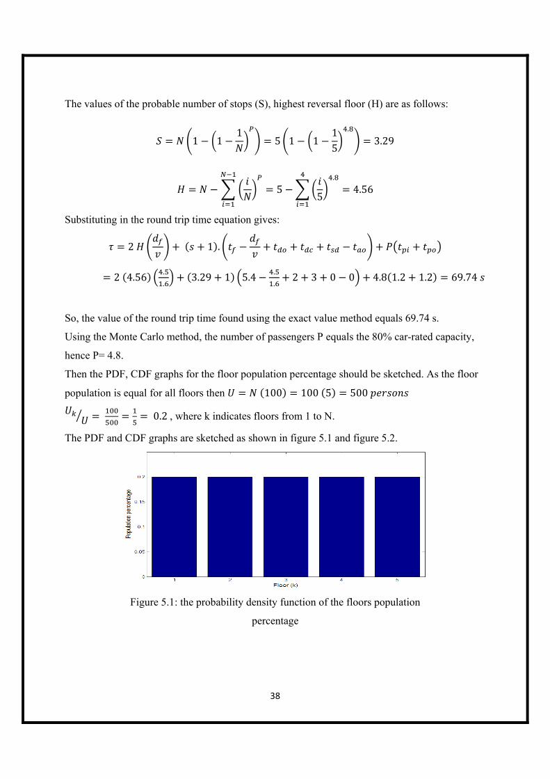
Then the PDF, CDF graphs for the floor population percentage should be sketched. As the floor
population is equal for all floors then 100 100 5 500
0.2, where k indicates floors from 1 to N.
The PDF and CDF graphs are sketched as shown in figure 5.1 and figure 5.2.
Figure 5.1: the probability density function of the floors population
percentage

39
Figure 5.2: The cumulative density function of the floors population
percentage
The next step is to generate five random numbers between (0-1), the random numbers generated
are: 0.391, 0.936, 0.12, 0.317, 0.081
By scanning the CDF, the random generated floors based on the floor population percentage are:
First floor, fifth floor, first floor, second floor and first floor. So there will be one stop on the first
floor, one stop on the second floor and one stop on the fifth floor. Therefore, the number of stops
equals three.
The kinematics time for this journey scenario is:
Where:
: is the transition time between the ground floor and the first floor.
: is the transition time between the first floor and the second floor.
: is the transition time between the second floor and the fifth floor.
: is the transition time between the fifth floor and the ground floor.
Since the top speed is attained in one floor journey the transition times are calculated as follows:
4.51.6
1.61
11
5.41
4.51.6
1.61
11
5.41
4.5 31.6
1.61
11
11.04
40
4.5 51.6
1.61
11
16.66
The kinematics time equals to:
5.41 5.41 11.04 16.66 38.52
The constant time for this journey scenario is calculated as follows:
3 2 3 4.8 1.2 1.2 26.52
The round trip time for one trial equal:
21.86 26.52 65.04
Using the Monte Carlo software tool, the round trip time found for one trial equal: 51.195 s
It is important to recall that the round trip time value found for one trial differ from trial to
another as the procedure is totally random and depends on the set of random numbers generated
each time.
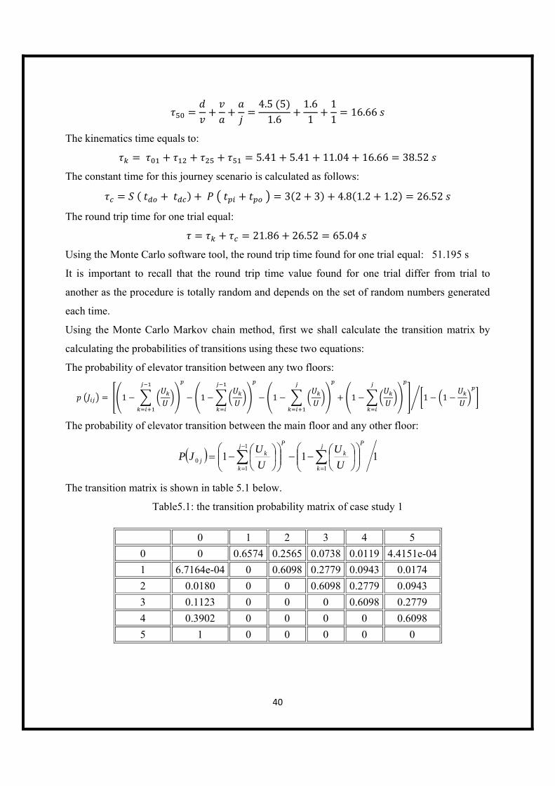
Using the Monte Carlo Markov chain method, first we shall calculate the transition matrix by
calculating the probabilities of transitions using these two equations:
The probability of elevator transition between any two floors:
1 1 1 1 1 1
The probability of elevator transition between the main floor and any other floor:
1111
1
10
Pj
k
k
Pj
k
kj U
U
U
UJP
The transition matrix is shown in table 5.1 below.
Table5.1: the transition probability matrix of case study 1
0 1 2 3 4 5
0 0 0.6574 0.2565 0.0738 0.0119 4.4151e-04
1 6.7164e-04 0 0.6098 0.2779 0.0943 0.0174
2 0.0180 0 0 0.6098 0.2779 0.0943
3 0.1123 0 0 0 0.6098 0.2779
4 0.3902 0 0 0 0 0.6098
5 1 0 0 0 0 0

41
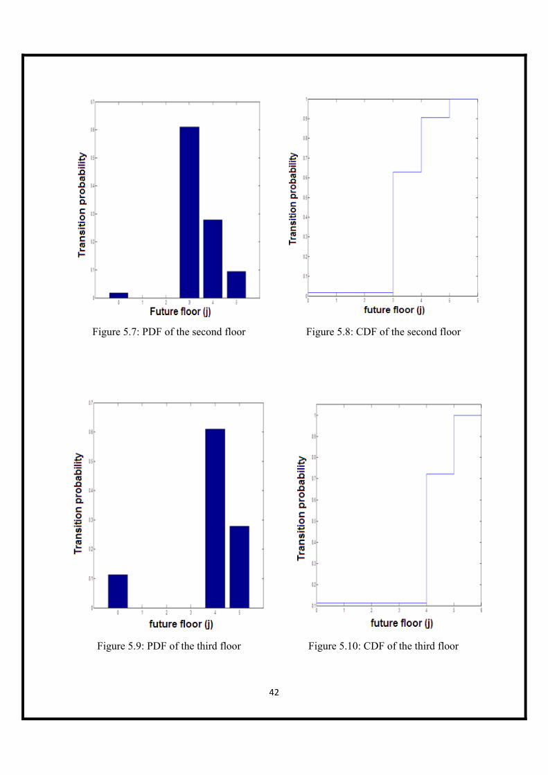
After that, PDF and CDF graphs should be sketched for each row of the matrix, they are shown
in figures below (figures 5.3- 5.14 ).
Figure 5.3: PDF of the ground floor Figure 5.4: CDF of the ground floor
Figure 5.5: PDF of the first floor Figure 5.6: CDF of the first floor
42
Figure 5.7: PDF of the second floor Figure 5.8: CDF of the second floor
Figure 5.9: PDF of the third floor Figure 5.10: CDF of the third floor

43
Figure 5.11: PDF of the fourth floor Figure 5.12: CDF of the fourth floor
Figure 5.13: PDF of the fifth floor Figure 5.14: CDF of the fifth floor

44
Afterwards, the first random number is generated, the first random number is 0.869. By scanning
the ground floor’s CDF we have the first random destination which is the second floor. Taking
another random number, we have 0.935, by scanning the second floor’s CDF we have the next
destination which is in this case is the fourth floor. Taking another random number we have
0.995 by scanning the fourth floor’s CDF we get the next destination which in this case is the
fifth floor. Taking another random number we have 0.691, by scanning the fifth floor CDF we
have the next destination which is the ground floor.
Now, the first journey scenario is generated; where the elevator will stop first at the second floor
then at the fourth floor then at the fifth floor before it turns back to the ground floor, hence we
number of stops for this journey equals three. Number of passengers equals three too.
The kinematics time for this journey scenario is:
Where:
: is the transition time between the ground floor and the second floor.
: is the transition time between the second floor and the fourth floor.
: is the transition time between the fourth floor and the fifth floor.
: is the transition time between the fifth floor and the ground floor.
Since the top speed is attained in one floor journey the transition times are calculated as follows:
4.5 21.6
1.61
11
8.225
4.5 21.6
1.61
11
8.225
4.5 11.6
1.61
11
5.41
4.5 51.6
1.61
11
16.66
The kinematics time equals to:
8.225 8.225 5.41 16.66 38.52
The constant time for this journey scenario is calculated as follows:
3 2 3 3 1.2 1.2 22.2

45
The round trip time for one trial equal:
38.52 22.2 60.72
Using the Monte Carlo Markov chain software tool, the round trip time found for one trial equal:
62.445 s. It is important to recall that the round trip time value found for one trial differ from
trial to another as the procedure is totally random and depends on the set of random numbers
generated each time.
Using the simulation software, we will get the results shown in the table 5.2 below.
Table 5.2: the simulation software results for the values of round trip time using MCMC and MC
methods for different number of trials
Number of Trials RTT using MCMC RTT using Monte Carlo
100 69.6813 65.4935
1000 69.7998 66.1725
10000 69.7188 67.6293
100000 69.736 68.9655
After that, the percentage of error for Monte Carlo Markov Chain method is calculated as
follows:
%
100%
Likewise, the percentage of error for Monte Carlo method is calculated as follows:
%
100%
The error percentage values are calculated and filled in table 5.3 below.

46
Table 5.3: percentage of error for Monte Carlo Markov chain method and Monte Carlo method
for case study 1
Number of Trials MCMC percentage of error Monte Carlo percentage of
error
100 0.086% 6.091%
1000 0.084% 5.117%
10000 0.032% 3.028%
100000 7.743 10 % 1.112%
The percentage of error functions is sketched and shown in figure 5.15 below.
Figure 5.15 : Percentage of error versus number of trials in log scale

47
5.2 Case study 2
Another example from a building is used to illustrate the use of Monte Carlo Markov chain
simulation. The parameters for a typical building with equal floor heights and equal floor
population are shown below.
1- Number of floors above the ground floor equals 10.
2- Car capacity is 8 persons.
3- Finished floor level to finished floor level (floor height) is 4.5 m.
4- Each floor population is 150 persons.
5- Rated speed is 1.6 m.s-1.
6- Rated acceleration is 1 m.s-2.
7- Rated jerk is 1 m.s-3.
8- Passenger alighting time equals 1.2 s.
9- Passenger boarding time equals 1.2 s.
10- Door opening time equals 2 s.
11- Door closing time equals 3 s.
12- Start delay is 0.
13- Advanced opening time is 0.
We will start with the exact solution; a check needs to be carried out to ensure that the elevator
will attain top speed in a one floor journey, as follows:
4.5
1 1.6 1.6 1
14.16
So the top speed of 1.6 m/s is attained in a one-floor journey. In this case the time taken to
complete a one-floor journey, tf will be:
4.51.6
1.61
11
5.4
The value of P based on 80% car-rated capacity is:
0.8 0.8 8 6.4

48
The values of the probable number of stops (S), highest reversal floor (H) are as follows:
1 11
10 1 1110
.
4.905
1010
.
9.096
Substituting in the round trip time equation gives:
2 1 .
2 9.096.
.4.905 1 5.4
.
.2 3 0 0 6.4 1.2 1.2
111.3996
So, the value of the round trip time found using the exact value method equals 111.3996 s.
Using the Monte Carlo method, the number of passengers P equals the 80% car-rated capacity,
hence P= 6.4.
Then the PDF, CDF graphs for the floor population percentage should be sketched. As the floor
population is equal for all floors then 150 150 10 1500
0.1, where k indicates floors from 1 to N.
The PDF and CDF graphs are sketched in figure 5.16 and figure 5.17 respectively.
Figure 5.16: The probability density function of the floors population percentage

49
Figure 5.17: The Cumulative density function of the floors population percentage
The next step is to generate five random numbers between (0-1), the random numbers generated
are: 0.093, 0.029, 0.455, 0.324, 0.113, 0.829, 0.845, 0.104, 0.466, 0.431
By scanning the CDF, the random generated floors based on the floor population percentage are:
First floor, first floor, fifth floor, fourth floor, second floor, ninth floor, ninth floor, second floor,
fifth floor and fifth floor. So there will be one stop on the first floor, one stop on the second
floor, one stop on the fourth floor, one stop on the fifth floor and one stop on the ninth floor.
Therefore, the number of stops equals five stops.
The kinematics time for this journey scenario is:
Where:
: is the transition time between the ground floor and the first floor.
: is the transition time between the first floor and the second floor.
: is the transition time between the second floor and the fourth floor.
: is the transition time between the fourth floor and the fifth floor.
: is the transition time between the fifth floor and the ninth floor.
: is the transition time between the ninth floor and the ground floor.
Since the top speed is attained in one floor journey the transition times are calculated as follows:
4.51.6
1.61
11
5.41

50
4.51.6
1.61
11
5.41
4.5 21.6
1.61
11
8.225
4.51.6
1.61
11
5.41
4.5 41.6
1.61
11
13.85
4.5 101.6
1.61
11
30.725
The kinematics time equals to:
5.41 5.41 8.225 5.41 13.85 30.725
69.03
The constant time for this journey scenario is calculated as follows:
5 2 3 6.4 1.2 1.2 40.36
The round trip time for one trial equal:
69.03 40.36 109.39
Using the Monte Carlo software tool, the round trip time found for one trial equal: 102.01 s
It is important to recall that the round trip time value found for one trial differ from trial to
another as the procedure is totally random and depends on the set of random numbers generated
each time.
Using the Monte Carlo Markov chain method, first we shall calculate the transition matrix by
calculating the probabilities of transitions using these two equations:
The probability of elevator transition between any two floors:
1 1 1 1 1 1
The probability of elevator transition between the main floor and any other floor:
Pj
k
k
Pj
k
kj U
U
U
UJP
1
1
10 11
The transition probabilities are calculated and filled in the transition matrix. The transition matrix
is shown in table 5.4 below.

51
Table 5.4: the transition probability matrix for case study 2
0 1 2 3 4 5 6 7 8 9 10
0 0 0.4905 0.2697 0.1378 0.0640 0.0262 0.0090 0.0024 4.1676e-04 3.3221e-05 3.9811e-07
1 8.1165e-07 0 0.4500 0.2691 0.1504 0.0770 0.0350 0.0135 0.0040 7.8194e-04 6.6919e-05
2 6.7731e-05 0 0 0.4500 0.2691 0.1504 0.0770 0.0350 0.0135 0.0040 7.8194e-04
3 8.4967e-04 0 0 0 0.4500 0.2691 0.1504 0.0770 0.0350 0.0135 0.0040
4 0.0049 0 0 0 0 0.4500 0.2691 0.1504 0.0770 0.0350 0.0135
5 0.0184 0 0 0 0 0 0.4500 0.2691 0.1504 0.0770 0.0350
6 0.0534 0 0 0 0 0 0 0.4500 0.2691 0.1504 0.0770
7 0.1304 0 0 0 0 0 0 0 0.4500 0.2691 0.1504
8 0.2808 0 0 0 0 0 0 0 0 0.4500 0.2691
9 0.5500 0 0 0 0 0 0 0 0 0 0.4500
10 1 0 0 0 0 0 0 0 0 0 0
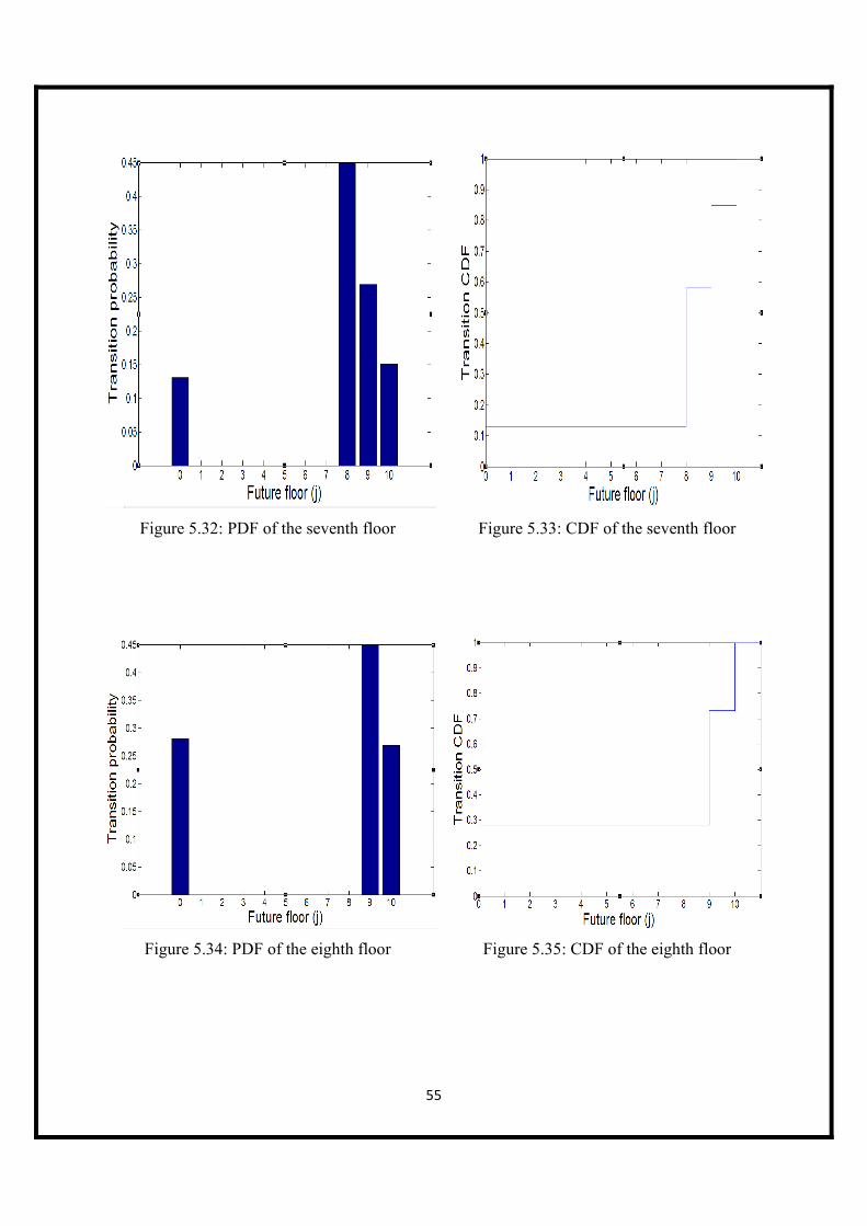
After that, PDF and CDF graphs should be sketched for each row of the matrix, they are shown
in figures below (figures 5.18- 5.39).
Figure 5.18: PDF of the ground floor Figure 5.19: CDF of the ground floor

52
Figure 5.20: PDF of the first floor Figure 5.21: CDF of the first floor
Figure 5.22: PDF of the second floor Figure 5.23: CDF of the second floor

53
Figure 5.24: PDF of the third floor Figure 5.25: CDF of the third floor
Figure 5.26: PDF of the fourth floor Figure 5.27: CDF of the fourth floor

54
Figure 5.28: PDF of the fifth floor Figure 5.29: CDF of the fifth floor
Figure 5.30: PDF of the sixth floor Figure 5.31: CDF of the sixth floor
55
Figure 5.32: PDF of the seventh floor Figure 5.33: CDF of the seventh floor
Figure 5.34: PDF of the eighth floor Figure 5.35: CDF of the eighth floor

56
Figure 5.36: PDF of the ninth floor Figure 5.37: CDF of the ninth floor
Figure 5.38: PDF of the tenth floor Figure 5.39: CDF of the tenth floor

57
Afterwards, the first random number is generated; the first random number is 0.684. By scanning
the ground floor’s CDF we have the first random destination which is the second floor. Taking
another random number, we have 0.492, by scanning the second floor’s CDF we have the next
destination which is in this case is the fourth floor. Taking another random number we have
0.999 by scanning the fourth floor’s CDF we get the next destination which in this case is the
tenth floor. Taking another random number we have 0.057, by scanning the tenth floor CDF we
have the next destination which is the ground floor.
Now, the first journey scenario is generated; where the elevator will stop first at the second floor
then at the fourth floor then at the tenth floor before it turns back to the ground floor, hence the
number of stops for this journey equals three. Number of passengers equals three too.
The kinematics time for this journey scenario is:
Where:
: is the transition time between the ground floor and the second floor.
: is the transition time between the second floor and the fourth floor.
: is the transition time between the fourth floor and the tenth floor.
: is the transition time between the tenth floor and the ground floor.
Since the top speed is attained in one floor journey the transition times are calculated as follows:
4.5 21.6
1.61
11
8.225
4.5 21.6
1.61
11
8.225
4.5 61.6
1.61
11
19.475
4.5 101.6
1.61
11
30.725
The kinematics time equals to:
8.225 8.225 19.475 30.725 66.65
The constant time for this journey scenario is calculated as follows:
3 2 3 3 1.2 1.2 22.2

58
The round trip time for one trial equal:
38.52 22.2 88.85
Using the Monte Carlo Markov chain software tool, the round trip time found for one trial equal:
109.61 s. It is important to recall that the round trip time value found for one trial differ from
trial to another as the procedure is totally random and depends on the set of random numbers
generated each time.
Using the simulation software, we will get the results shown in the table 5.5 below.
Table 5.5: the simulation software results for the values of round trip time using MCMC and MC
methods for different number of trials for case study 2
Number of Trials RTT using MCMC RTT using Monte Carlo
100 108.3428 s 106.0108 s
1000 110.3737 s 107.9322 s
10000 111.4742 s 109.5695 s
100000 111.381 s 110.3372 s
After that, the percentage of error for Monte Carlo Markov Chain method is calculated as
follows:
%
100%
Likewise, the percentage of error for Monte Carlo method is calculated as follows:
%
100%
The error percentage values are calculated and filled in table 5.6 below.
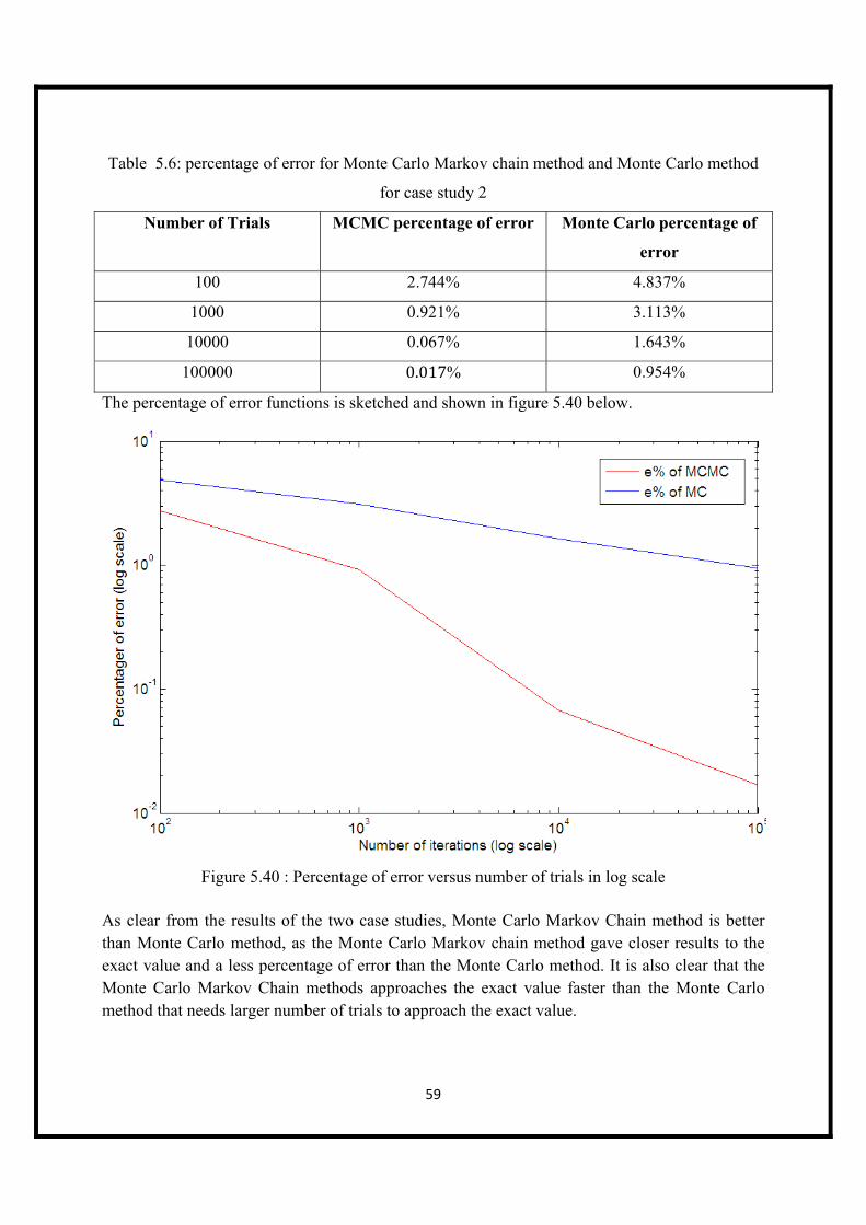
59
Table 5.6: percentage of error for Monte Carlo Markov chain method and Monte Carlo method
for case study 2
Number of Trials MCMC percentage of error Monte Carlo percentage of
error
100 2.744% 4.837%
1000 0.921% 3.113%
10000 0.067% 1.643%
100000 0.017% 0.954%
The percentage of error functions is sketched and shown in figure 5.40 below.
Figure 5.40 : Percentage of error versus number of trials in log scale
As clear from the results of the two case studies, Monte Carlo Markov Chain method is better than Monte Carlo method, as the Monte Carlo Markov chain method gave closer results to the exact value and a less percentage of error than the Monte Carlo method. It is also clear that the Monte Carlo Markov Chain methods approaches the exact value faster than the Monte Carlo method that needs larger number of trials to approach the exact value.

60
5.3 Conclusions and future work
The design of the elevator systems involves the selection of the number, capacity and speed of
the elevators to achieve the required performance, and it relies on the calculation of the round
trip time, as the round trip time gives a good measure for both the quantity and quality of service,
as both the interval and the handling capacity calculations depends on the round trip time value.
Therefore, it is important to derive accurate and easy methods to calculate the round trip time.
The Monte Carlo Markov chain simulation method was introduced as a methodology to arrive at
the value of the round trip time during incoming traffic conditions in the simplest case which
assumes equal floor population, equal floor heights, one entrance floor and a top speed that is
attained in a one floor journey. The advantages of the Monte Carlo Markov chain method is the
simplicity of programming and accuracy.
Also, the Monte Carlo simulation method was introduced as a simulation method for calculating
the round trip time. Monte Carlo Markov chain simulation method is better than Monte Carlo
simulation method as the first one is faster and needs less number of trials to approach the exact
value, and it also gives a less percentage or error.
Furthermore, If any or a combination of the general assumptions of; equal floor population, equal
floor height, single entrance and the top speed attained in a one floor journey, was dropped,
Monte Carlo Markov chain simulation method can be easily developed to cover all of these
cases. However, the analytical method cannot deal with a combination of these special cases as
the problem becomes very complicated. So, the development of the Monte Carlo Markov chain
simulation method can give a good alternative for the analytical method for calculating the round
trip time when any or all of the general four assumptions does not exist.
Likewise, in the future Monte Carlo Markov chain simulation method can be developed to a
Markov Chain method which only depends on the Markov chains to arrive at the value of the
round trip time depending only on the steady state probabilities.

61
References
[1] "Laying the foundation for today's skyscrapers". San Francisco Chronicle. August 23,
2008.
[2] N. A. Alexandris. “Statistical Models in Lift Systems”, Ph.D. Thesis, University of
Manchester, Institute of Science and Technology, 252 p., 1977.
[3] H. Hakonen. “Simulation of Building Traffic and Evacuation by Elevators”, Licentiate
Thesis, Helsinki University of Technology, 117 p., 2003.
[4] S. P. Meyn and R. L. Tweedie. Markov Chains and Stochastic Stability. London: Springer-
Verlag, 1993. ISBN 0-387-19832-6.
[5] Dodge, Y. (2003) The Oxford Dictionary of Statistical Terms, OUP. ISBN 0-19-920613-
9 (entry for "Markov chain")
[6] Usatenko, O. V.; Apostolov, S. S.; Mayzelis, Z. A.; Melnik, S. S. (2010) Random finite-
valued dynamical systems: additive Markov chain approach. Cambridge Scientific
Publisher. ISBN 978-1-904868-74-3
[7] Curtis Roads (ed.) (1996). The Computer Music Tutorial. MIT Press. ISBN 0-262-18158-
4.
[8] Lutfi Al-Sharif. Deriving the round trip time for the general case under incoming traffic
conditions. 2011; 6-9.
[9] Lutfi Al-Sharif, Husam M Aldahiyat, Laith M Alkurdi. The use of Monte Carlo simulation
in evaluating the elevator round trip time under up-peak traffic conditions and conventional
group control,2012, 319-328.
[10] http://www2.ju.edu.jo/sites/Academic/l.sharif/Material/0908589%20Elevator%20Traffic%20Anal
ysis%20Design%20and%20Control/02%20Calculating%20the%20Round%20Trip%20Time/3%20Ro
und%20Trip%20Time%20calculations%20revision%2010%20%20111010.pdf.

62
Appendix
Matlab GUI Code for the software tool
N = str2num(get(handles.edit1,'String')); u = str2num(get(handles.edit2,'String')); Pa = str2num(get(handles.edit3,'String')); tpi = str2num(get(handles.edit4,'String')); tpo = str2num(get(handles.edit5,'String')); tdo = str2num(get(handles.edit6,'String')); tdc = str2num(get(handles.edit7,'String')); U = u*N; set (handles.edit8,'String',num2str(U)); %--------------------------------------------------------------- %transition Matrix (A) Construction %--------------------------------------------------------------- A = zeros(N+1); A(N+1,1)= 1; for i=1:N for j = 1:N+1 if (i<j) if(i==1) c1=0;c2=0; for k=1:j-2 c1 = c1 + u/U; end for k=1:j-1 c2 = c2 + u/U; end A(i,j) = ((1-c1)^Pa - (1-c2)^Pa); else k1=0;k2=0;k3=0;k4=0; for k=i:j-2 k1 = k1 + u/U; end for k=i-1:j-2 k2 = k2 + u/U;

63
end for k=i:j-1 k3 = k3 + u/U; end for k=i-1:j-1 k4 = k4 + u/U; end A(i,j) = ((1-k1)^Pa - (1-k2)^Pa -(1-k3)^Pa +(1-k4)^Pa)/(1-(1-u/U)^Pa); end end end end for i = 2:N Row_sum = 0; for k = 2:N+1 Row_sum = Row_sum + A(i,k); end A(i,1) = 1- Row_sum ; end A set(handles.uitable1, 'Data', A); %--------------------------------------------------------------- %steady state Probability (pi) %--------------------------------------------------------------- IM = A-eye(N+1); IM(:,N+1)= ones(N+1,1); R = zeros(1,N+1); R(1,N+1) = 1; X = R*inv(IM); set(handles.uitable2, 'Data', X); %--------------------------------------------------------------- %Analytical Solution %--------------------------------------------------------------- df = str2num(get(handles.edit18,'String')); v =str2num(get(handles.edit19,'String')); a = str2num(get(handles.edit20,'String'));

64
je = str2num(get(handles.edit21,'String')); tf = df/v + v/a + a/je ; tv = df/v ; ts = tf - tv + tdo +tdc; S2 = N*(1-(1- (1/N))^Pa); set (handles.edit25,'String',num2str(S2)); im2=0; for k =1:N-1 im2 = im2 + (k/N)^Pa; end H = N - im2; T2 = 2*H*tv + ts*(S2+1) + Pa*(tpi +tpo); set (handles.edit26,'String',num2str( T2 )); %---------------------------------------------------------------%simulation #1 : MARKOV simulation %--------------------------------------------------------------- Nrpt = str2num(get(handles.edit31,'String')); Tau_sum = 0; for repeat = 1:Nrpt s=0; state1in = 0; state2 = 1948; Tk = 0; while(state2 ~= 0) s = s+1; state1 = state1in +1; rndm = rand(1); summ = 0; for k =1:size(A,1)+1 if summ >= rndm state2 = k-2 ; break; else

65
summ = summ + A(state1 , k); end end d = abs(state2 - state1in)*df; direction = (state2 - state1in); %------------------------------------------------------------ %time from floor to floor %------------------------------------------------------------ if d >= (((a^2)*v + (v^2)*je)/(a*je)) t_a2b = d/v + v/a + a/je; elseif d < (2*a^3/je^2) t_a2b = (32*d/je)^(1/3); else t_a2b = a/je + ((4*d/a + (a/je)^2)^(0.5)); end %------------------------------------------------------------ Tk = Tk + t_a2b; state1in = state2; end t_constant = Pa*(tpi + tpo) + (s)*(tdo+tdc); Tau = t_constant + Tk; Tau_sum = Tau_sum + Tau; end avg_Tau = Tau_sum / Nrpt set (handles.edit33,'String',num2str( avg_Tau )); %--------------------------------------------------------------- %simulation #2 :Monte Carlo %--------------------------------------------------------------- Tau2_sum = 0; B = zeros(N+1);% # Passengers matrix T = zeros(N+1);%# transitions matrix for repeat = 1:Nrpt Random = sort( rand(1,Pa) );

66
Randomx = 0; Floor = [0, floor(N*Random +1) ]; transition = 0; for k = 1:Pa if ( Floor(k+1) ~= Floor(k) ); transition(length(transition)+1) = Floor(k+1); end end d= [diff(transition),max(transition)]*df; %--------------------------------------------------------- %time from Floor to Floor %--------------------------------------------------------- Tk2 = 0; for ln = 1: size(d,2) d_ln = d(ln); if d_ln >= ((a^2)*v + (v^2)*je)/(a*je) t_a2b = d_ln/v + v/a + a/je ; elseif d_ln < (2*a^3/je^2) t_a2b = (32*d_ln/je)^(1/3); else t_a2b = a/je + ((4*d_ln/a + (a/je)^2)^(0.5)); end Tk2 = Tk2 + t_a2b; end %------------------------------------------------------------ Splus1 = size(transition,2); t_constant2 = Pa*(tpi + tpo) + (Splus1)*(tdo+tdc); Tau2 = t_constant2 + Tk2; Tau2_sum = Tau2_sum + Tau2; %------------------------------------------------------------ %Monte Carlo simulated Matrix %------------------------------------------------------------ %B = zeros(N+1); initially transition(length(transition)+1) = 0; %B is the number of passengers moved from floor =(row-1) to floor =(column-1) %T is the number of transitions from floor =(row-1) to floor =(column-1) for j=1:length(transition)-1

67
B(transition(j)+1,transition(j+1)+1) = B(transition(j)+1,transition(j+1)+1) + sum(Floor == transition(j+1)); T(transition(j)+1,transition(j+1)+1) = T(transition(j)+1,transition(j+1)+1) + 1; end %B %T %------------------------------------------------------------ %------------------------------------------------------------ end B T=T/Nrpt set(handles.uitable4, 'Data', T); %------------------------------------------------------------ %------------------------------------------------------------ avg_Tau2 = Tau2_sum / Nrpt set (handles.edit34,'String',num2str( avg_Tau2 )); set (handles.text44,'String','ATH'); %------------------------------------------------------------ %------------------------------------------------------------ %Markov from Monte Carlo %------------------------------------------------------------- %transition Matrix (P) Construction %------------------------------------------------------------- for i=1:N+1 Added(i)= sum(T(i,:)); %T(i,1)=T(i,1) + 1- sum(T(i,:)); end Production = 1/min(Added); T(2:N+1,:)=T(2:N+1,:)*Production; P = T %set(handles.uitable7, 'Data', A); %------------------------------------------------------------- %simulation #1 : MARKOV simulation %------------------------------------------------------------- Nrpt = str2num(get(handles.edit31,'String')); Tau_sum = 0; for repeat = 1:Nrpt

68
s=0; state1in = 0; state2 = 1948; Tk = 0; while(state2 ~= 0) s = s+1; state1 = state1in +1; rndm = rand(1); summ = 0; for k =1:size(P,1)+1 if summ >= rndm state2 = k-2; break; else summ = summ + P(state1 , k); end end d = abs(state2 - state1in)*df; direction = (state2 - state1in); %------------------------------------------------------------ %time from floor to floor %------------------------------------------------------------ if d >= (((a^2)*v + (v^2)*je)/(a*je)) t_a2b = d/v + v/a + a/je; elseif d < (2*a^3/je^2) t_a2b = (32*d/je)^(1/3); else t_a2b = a/je + ((4*d/a + (a/je)^2)^(0.5)); end %------------------------------------------------------------ Tk = Tk + t_a2b; state1in = state2; end t_constant = Pa*(tpi + tpo) + (s)*(tdo+tdc); Tau = t_constant + Tk; Tau_sum = Tau_sum + Tau; end avg_Tau = Tau_sum / Nrpt
Related Documents