Filtering, modulation and diffraction: an introduction to Fourier optics

CASEAN 2013, Phnom Penh 2013-11-12

FILTERING, MODULATION AND DIFFRACTION:

FROM SIGNAL PROCESSING TO FOURIER OPTICS

Roberto Coisson

a) Department of Physics and Earth Sciences, University of Parma

area delle Scienze 7/A, 43100 Parma, Italy

E-mail: [email protected]

Historically, the concepts of optical image processing were developed inanalogy with the processing of time signals. It is therefore of interest, from adidactic point of view, to present the various operations on one-dimensionaland two-dimensional signals in parallel, showing how “modulation”corresponds to “diffraction”, and “filtering” to “spatial filtering”. Thisapproach shows how the concepts related to the Fourier Transform canprovide a simple and coherent framework for processing of both time signalsand optical images.

INTRODUCTION

Diffraction, filtering, angular spectrum, spatial filtering, heterodyne,holography, are basic concepts in Signal Processing, Optics and in ImageProcessing, and in general in all wave phenomena. The commonmathematical background of all these phenomena is given by the FourierTransform: in on dimension in case of signal processing and radiocommunications, in two dimensions in the case of Image Processing,Diffraction and spatial filtering.

In the teaching to advanced students it is therefore useful to compare one-and two-dimensional phenomena, as the 1D case is more intutivelyunderstandable, and helps to make the further generalisation to the 2D case.In fact, historically, the concepts of “Fourier Optics” and Image Processinghave been developed in analogy with the already existing radiofrequencytechnologies.

Before the course it is necessary to give the students a bief practicalintroduction to the Fourier Transform, without too much formalism anddetailed demonstrations of theorems. This is briefly outlined in Appendix A.

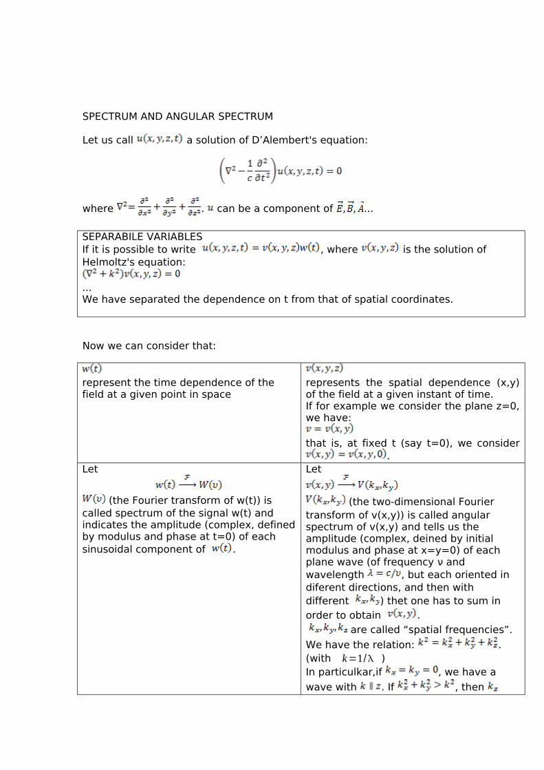
SPECTRUM AND ANGULAR SPECTRUM

Let us call a solution of D’Alembert's equation:

where . can be a component of ...

SEPARABILE VARIABLESIf it is possible to write , where is the solution of Helmoltz's equation:

...We have separated the dependence on t from that of spatial coordinates.

Now we can consider that:

represent the time dependence of the field at a given point in space

represents the spatial dependence (x,y)of the field at a given instant of time.If for example we consider the plane z=0,we have:

that is, at fixed t (say t=0), we consider.

Let

(the Fourier transform of w(t)) is called spectrum of the signal w(t) and indicates the amplitude (complex, definedby modulus and phase at t=0) of each sinusoidal component of .

Let

(the two-dimensional Fourier transform of v(x,y)) is called angular spectrum of v(x,y) and tells us the amplitude (complex, deined by initial modulus and phase at x=y=0) of each plane wave (of frequency ν and wavelength , but each oriented in diferent directions, and then with different ) thet one has to sum in order to obtain . are called “spatial frequencies”.

We have the relation: .(with k=1/ )In particulkar,if , we have a

wave with . If , then

turns out to be imaginary and then the dependence of is of the type

, which means that these waves which have a spatial frequency

are

exponentially attenuated in the direction z are called “evanescent waves”.

We call MODULATION the operation by which w(t) is multiplied by a function m(t)(in general complex). In this way the spectrum is modified: if and indicate the non-modulated functions :

where is the Fourier transform of, and * indicates the operation of

convolution..

DIFFRACTION. Let us consider now a wave with components with

(which means that they propagate in the positive z direction). If in the plane z=0 there is a screen which attenuates the amplitude by a factor (t compleX, |t|<1) (for example a transparency), the angular spectrum of the wave in the region z>0 will be modified:

where e

.

In particular, if is a monochromatic plane wave with , we have

and then

.The angular spectrum gives us the distribution of directions of the component plane waves. .

If we put a lens on a plane z = constant > 0 (that is, after the transparency), at each point of its focal plane will come to focus one of the component plane waves, having a given direction. The light intensity at that point will depend on the amplitude of the corresponding plane wave component.

Let us take for simplicity a wave such that, so that the angle formed with th z

axis is very small. That plane wave component will come to focus at a point

with y=0 and .

At each point of the focal plane , the amplitude of the wave will be proportional to the corresponding component of the angular spectrum:

.

Or (which is the same) we can take off the lens and observe the distribution of the wave at a large distance (how large

has to be defined) as a function of e .

This amplitude distribution resulting from the diffraction from the screen , observed on the focal plane of a lens or “at infinity” is called FRAUNHOFER. DIFFRACTION

FILTER. We call filter an instrument which multiplies the spectrum by a function (in general complex, and usually of modulus <1). This modifies the temporal dependence of the signal :

A particular case: an ideal narrowband filter has a monochromatic output of frequency (for any function containing that frequency).

SPATIAL FILTER (or“anguar filter): we call spatial filter an instrument which multiplies (by a given function )

the angular spectrum of a wave.This modifies the distrubution of component waves:

It can be realised, for example, in this way:

The screen, with attenuation

is placed on the

common focal plane of the two lenses.A particular case: the screen is opaque and with a pinhole at . Then

. The output wave is a

plane wave with .

EXAMPLES

SPECTRA of MODULATED SIGNALS FRAUNHOFER DIFFRACTION

In all following cases we consider a screen on the plane z=0, on which is incident a monochromatic plane wave with , and we will calculate the angular spectrum of the wave coming out of the screen , which is equivalent to say that we consider the Fraunhofer diffraction regime (and to find the observed intensity we do the modulus square).

1) Spectrum of sinusoidal signal of limited duration :

If we call “bandwidth” tghe frequency interval in which is appreciably different from zero, we have the indeterminacy relation : . This is valid in general, as a theorem on Fourier Transforms: in Quantum Mechanics this corresponds to the fact that a measurement of energy which lasts a time has an

uncertainty .

1) Fraunhofer Diffraction from a slit, having infinite length in the direction y and of width a in the direction x:

The functions are the same as in the temporal case (on the left column), except that the sinc function is centredaround

The narrower the slit, the wider is the diffraction pattern. Also in this case there is an indeterminacy relation : (in Quantum Mechanics complementarity position-momentum).In other words, if a plane wave encounters a slit of width , it comes

out with an angular divergence

(“diffraction angle”)).1’) Fraunhofer diffraction from a rectangular aperture:

1’’) Fraunhofer diffraction from a circular hole of radius :

2) Spectrum of a sequence of two sinusoidal trains, each of duration a and with an interval d between the centres of the two trains.Same problem as the diffraction from two slits (see right column), except that in

2) Fraunhofer Diffraction from two slits (infinite, parallel):

place of and the spectrum is centred around ν0 instead of zero.

Taking into account that the intensity of the diffraction pattern is and that the angle that a plane component of the angular spectrum forms with the z axis is (if )

, we find that the angle

formed by two successive maxima (angular “distance” between fringes) is

.3) If a signal is formed by an infinite series of short pulses, with interval , its spectrum is composed of an infinite number

of terms with frequencies all

with the same initial phase.

where is the “Dirac Comb”.On the other hand, we can say that if we take many sinusoidal signals with the same amplitude and frequencies and they start all with the same phase , we obtain a signal composed of pulses repeatedat intervals , each of very short duration: (the more components, the shorterthe pulses, as can be seen on point 4 below). This is the principle of “mode-locking” of lasers.

3) Diffraction from an ideal grating (infinite number of slits, with distances , and of width )

That means that from the grating, (illuminated with monochromatic light

, plane with perpendicular to

the grating ( ) comes out:1 plane wave which continues the incident one ( ) (diffraction of order zero)2 plane waves forming with z an angle

(diffracted waves of first order)

2 plane waves forming with z an angle

(2° order)

etc..4) -.. (to be done as an exercise, in analogy with the column on the right)

4) Grating

Remark the dependence from the

parameters ; also remark that for

, we obtain the previous

case.5) Spectrum of a sinusoidal signal (freq. ) amplitude modulated at freq. (i.e. multiplied by a real factor of type

):

5) Diffraction from a grating having a continuously variable attenuation, a sinusoid function of x (could be done for ex. With a photographic plate)).Analogous of the case on the left column. Conclusion: in such a grating there are only 3 diffracted waves: order zero and order +1 and -1.

6) Spectrum of a sinusoidal signal (freq. modulated in phase at freq. , that is with

( real constant):

Let us consider thel case ; then

It is like the previous case , only with instead of . The two “sidebands” are then

out of phase by with respect to the

“carrier” .

6) -Diffraction from a “phase grating”, i.e. A transparent sheet with thickness described by a sinusoidal function of x,so that is imaginary:

where is the period of the

gratingIf we can make the same approximation as in the case on the left column, and obtain the same result. .As on te diffraction pattern we see the intensity, we do not notice thatthe “sidebands” are out of phase, and then the pattern looks the same as in case 5 (amplitude sinusoidal grating).But if it is not true that , other sidebands (higher orders)appear.For a certain value of the modulation β it even happens that the order zero disappears.

Representing carrier and sidebands as rotating vectors, amplitude and phase modulation can be represented:

(the dotted lines represent the resulting modulation vector)HETERODYNE DEMODULATION. If a sinusoidal signal (“carrier”) is modulated by a function , and we want to find m(t) (or o a ), this operation is called “demodulation”. .

HOLOGRAPHYif a wavefront modulated in phase, the intensity that we see does not give us information about the modulation. It is therefore necessary to superimpose

1) If m(t) is real (amplitude modulation) we

can obtain averaged over times i

but where is the highest frequency

contained in .( ) We get

and, averaging, .

another wave, for example a plane wave, in order to “demodulate” and observe the “signal” (which is the formof the wavefront, giving us the form of the scattering object that constitutes the source of the wavefront).

Example:In-line Hologram of a point:Fresnel zones are formed on the recording plane.When illuminated by a plane wave, these converge or diverge and seem to come from the scatterinhg point [draw sketch].

PARTIAL COHERENCE

Signals, wavefronts and images are often not completely coherent, so it is convenient to give an idea of the effects of partial coherence. As a preliminary, a brief summary about Stochastic Functions is necessary, and a scheme is given in Appendix B.

Examples, just to give two suggestions:

Mode Locking

The FT of a “Dirac Comb” is a Dirac Comb: that means that if the spectrum of a signal is a sum of equally spaced narrow peaks, the signal is a series of short pulses. From the convolution theorem, the wider is the range of the spectrum, the shorter are the single pulses.

But if the phases of each frequency component are random, the signal is fluctuating with a constant average intensity. Only making the autocorrelation the periodicity is retrieved.

The “Mode Locking” of a laser is just the phase-locking of the various oscillating frequencies.

Diffraction from a grating:

In the simple case when the autocorrelation is “separable”, the incoming wavefront has an autocorrelation (or coherence function)

v(x,X;z=0-)=u(x)w(X)

the grating of width L and period d is g(x)=(rect(x/a)*Ш(x/d)) rect(x/L)

after the grating, v(x,X,z=0+)=g(x)u(x)w(X)

and then the angular autocorrelation

V(k,K)=W(k)(sinc(LK)*(sinc(aK)Ш(dK))*U(K)

A table of properties and particular cases of Fourier Transforms (adapted from Wikipedia)

properties

1 linearity

2 Shift in time

3 Shift in frequency

4 scaling

5 Inverse transform

6Derivative becomes

multiplication

7

8 Convolution Theorem

9 Convolution Theorem。

Useful functions (or generalised functions):

rect(x)=1 for -1/2<x<1/2, =0 elsewhere

sinc(x)=sin(πx)/(πx)

h(t)=1 for x>0, =0 for x<0 Heaviside's step function

δ(x) Dirac's delta function (a peak “very narrow and very tall”): it is the unity of convolution:

Ш(x)= (sum from -infinity to +infinity)

multiplication by Ш(x) results in a sampling, convolution with Ш(x) produces a periodic function

Appendix A

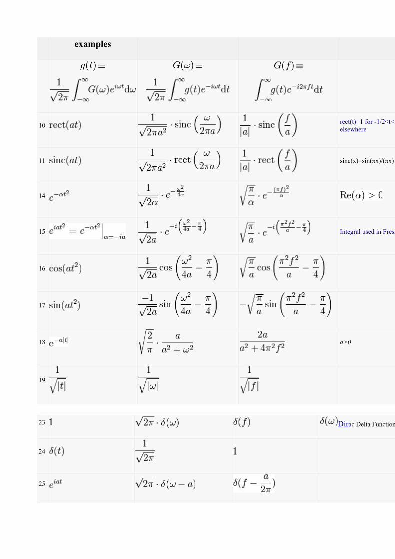
examples

10rect(t)=1 for -1/2<t<1/2, =0

elsewhere

11 sinc(x)=sin(πx)/(πx)

14

15 Integral used in Fresnel diffraction

16

17

18 a>0

19

23 Dirac Delta Function

24

25

26Remember that：

27

28 。

29

30 .

31 sgn(t)=-1 for t<0, =1 for t>0.

32 u(t) Heaviside step function

33 ，(a>0)

34 （Dirac comb）

Appendix B

Stochastic functionsa brief list of concepts

A stochastic function (SF) of a variable x is an ensemble of functions, each called a “realisation” of the SF.The FT F(u) of a SF f(x) is a SF where each realisation is the FT of a realisation of the SF.The modulus square of the FT is called “power spectrum”:The “ensemble average” m(x)=<f(x)> is the average of all the realisations at point x.“Autocorrelation” is Rf(x_1,x_2)=<f(x_1)'f(x_2)>A SF is “stationary” if Rf(x_1,x_2) is only a function of x_1-x_2=ξ, and “ergodic” if the ensemble average is = average in x.

In signal processing usually the variable is the time t, and we deal with stationary Sfs.image processing and diffraction with partially coherent light, we have usually non-stationary Sfs.

For stationary Sfs:Wiener-Khinchin theorem: FT(Rf(ξ))=PS(f(x) the power spectrum of f(x) is the FT ofits autocorrelation.

Generalisation for non-stationary Sfs:FTRf(x-ξ/2,x+ξ/2)=RFTf(u-v/2,u+v/2) where u is the transformed variable of ξ and vof x, explicitly:

∫∫−∞

+∞

f (x−ξ/2) ' f (x+ξ/2)exp (−i(xv+ξu))udxd ξ=∫∫−∞

+∞

F(u−v /2) ' F(u+v /2)du dv