FILM CONDENSATION OF LIQUID METALS PRECISION OF MEASUREMENT

FILM CONDENSATION OF LIQUIDMETALS - PRECISION OF MEASUREMENT

Stanley J. WilcoxWarren M. Rohsenow

Report No. DSR 71475-62

Contract No. GK 1113

Department of MechanicalEngineeringEngineering Projects LaboratoryMassachusetts Institute of Technology

April 1969

ENGINEERING PROJECTS LABORATORY,NGINEERING PROJECTS LABORATOR'

4GINEERING PROJECTS LABORATO'FINEERING PROJECTS LABORAT'

NEERING PROJECTS LABORK'EERING PROJECTS LABOR

ERING PROJECTS LABO'RING PROJECTS LAB'

ING PROJECTS LA-iG PROJECTS I3 PROJECTS

PROJECTFROJEC-

9JE(

TECHNICAL REPORT NO. 71475-62

FILM CONDENSATION OF LIQUID METALS - PRECISION OF

MEASUREMENT

by

Stanley J. Wilcox

Warren M. Rohsenow

Sponsored by

National Science Foundation

Contract No. GK 1113

APRIL 1969

Engineering Projects LaboratoryDepartment of Mechanical EngineeringMassachusetts Institute of Technology

-2-

FILM CONDENSATION OF LIQUID METALS - PRECISION OF MEASUREMENT

by

Stanley J. WilcoxWarren M. Rohsenow

ABSTRACT

Major differences exist in results published by investigatorsof film condensation of liquid metal vapors. In particular, thereported dependence of the condensation coefficient on pressure hasraised questions about both the precision of the reported data andthe validity of the basic interphase mass transfer analysis.

An error analysis presented in this investigation indicates thatthe reported pressure dependence of the condensation coefficient athigher pressures is due to an inherent limitation in the precision ofthe condensing wall temperature measurement. The magnitude of thislimitation in precision is different for the various test systemsused. The analysis shows, however, that the primary variable affectingthe precision of the wall temperature measurement is the thermal con-ductivity of the condensing block. To verify the analysis, potassiumwas condensed on a vertical surface of a copper condensing block.The copper block was protected from the potassium with nickel plating.Condensation coefficients near unity were obtained out to higher pres-sures than those previously reported for potassium condensed withstainless steel or nickel condensing blocks. These experimentalresults agree with the prediction of the error analysis.

In addition, a discussion of the precautions used to eliminatethe undesirable effects of both non-condensable gas and improperthermocouple technique is included.

It is concluded from the experimental data and the error analysisthat the condensation coefficient is equal to unity and that thepressure dependence reported by others is due to experimental error.

-3-

ACKNOWLEDGEMENTS

The authors are indebted to Professors P. Griffith, R.E.

Stickney, J.W. Rose and B.B. Mikic for many fruitful discussions.

This work was sponsored in part by the National Science

Foundation under Contract No. GK 1113 and sponsored by the Division

of Sponsored Research at M.I.T.

-4-

TABLE OF CONTENTS

Page

TITLE .....................

ABSTRACT ..................

ACKNOWLEDGMENTS ...........

TABLE OF CONTENTS ...-.....

LIST OF TABLES AND FIGURES

NOMENCLATURE .............

I. INTRODUCTION .........

II. THEORY ...............

III. EXPERIMENTAL APPARATUS

3.1 Test Condenser --

3.2 Second Condenser

3.3 Thermocoupls ...

IV. OPERATING PROCEDURE --

SAMPLE-DATA AND CALCUL

GENERAL-DATA AND CALCU

ERROR ANALYSIS .......

7.1 Sensitivity of a

.TED RESULTS.......

.ATED RESULTS.----

to errors in (T-

... ... .. ... ..

.. . . . .. . . .a

............--.... a

.......---------..

.. . . . .. . . .a

-- - - - -. - - -0

-. - - - -- . - -a

.. . . . .. . . .0

.. . . . .. . . .0

.........o........

7.2 Constant Error for each Assembly of a System ........

7.3 Distribution of Measured Temperatures inThermocouple Hole ..................................

7.4 Distribution of Possible Wall TemperatureMeasurements .......................................

7.5 Exclusion of Data Indicating T > T ; Calculationof E(T s) and E(a) .................................

VIII.EFFECT OF CONDENSING FLUID ..................- ---.--- .--.-

IX. EXPERIMENTS USING SECOND CONDENSER ...............---------

1

2

3

4

6

8

10

11

15

15

15

16

18

19

20

22

22

23

24

26

29

33

34

V.

VI.

VII.

-5-

Page

X. DISCUSSION ................... 35

XI. CONCLUSIONS ................................................ 37

REFERENCES ..................................................... 38

APPENDICES ..................................................... 41

A. Description of Equipment .................... 41

B. Tabulated Data and Results ............................ 48

C. Thermocouple Preparation and Use ...................... 52

D. Simplified Derivation of Temperature Distributionat Wall............................................. 61

E. Additional Analysis of Error ............ 70

F. Additional Information on Effect of Second Condenser .. 77

G. Listing of Computer Programs ...... ................... 78

H. Theoretical Effect of Non-Condensable Gas on theCondensation Coefficient .............................. 87

-_ - _-IM M M MINMIN IM11ililu 01llil

-6-

LIST OF TABLES AND FIGURES

Page

TABLE

I Tabulated Results 49

II Tabulated Data - Sheet 1 50

III Tabulated Data - Sheet 2 51

Figure

1 Fundamental Diagram for Film Condensation 93

2 Schematic of Natural Convection Loop 94

3 Sectional View of Test Condenser 95

4 Data and Results (Run 3 - Series 1) 96

5 Data and Results (Run 18 - Series 3) 97

6 Survey of Condensation Coefficient Data 98

7 Condensation Coefficient vs. (Tv T S) 99

8a Typical Hole of Radius "r" 100

8b Simplified, Linear Temperature Drop Impressed AcrossHole 100

8c Gaussian Distribution of Temperature Measurementsin Hole 100

9 Schematic Representation of Distribution in Holesand at Wall 101

10 Probability Density Function at Wall 102

11 Effect of Pressure on (T - T ) and (T - T ) 103v s S W

12 Distribution of Condensate Surface Temperature 104

13 Expected Value of {(T - T )/(q/A)] vs. Actual Value{(T - T )/(q/A)] v s 105

v S

14 E(r) and Data vs. Pv 106

15 Predicted Distribution of Data 107

-7-

Figure Page

16 Effect of Fluid on E(cX) 108

17 E(') vs. Pv for Water 109

18 Effect of 2nd Condenser at 11,0.02 atm. 110

Al Natural Convection Loop 111

A2 Loop During Construction 111

A3 Old and New Apparatus 111

A4 Elements for Test Section 111

A5 Test Section after Brazing 112

A6 Assembling of Top 112

A7 Loop with Auxiliaries 112

A8 Protective Drum in Place 112

Cl Immersion Test with Homogeneous Thermocouple 113

C2 Immersion Test with Inhomogeneous Thermocouples 114

C3 Heat Treatment of Chromel-Alumel Thermocouples 115

C4 Set-up Used in Tests of Homogeneity 116

El Effect of T Data-Series 1 117v

E2 Effect ot T Data-Series 2 118v

E3 Effect of T Data-Series 3 119v

Fl Effect of 2nd Condenser at '\O.06 atm. 120

-8-

NOMENCLATURE

A area

c heat capacity

E(z) Expected Value of z

f(z) density function for variable z

g gravitational acceleration

h latent heat of vaporization

h' latent heat which includes change of enthalpy due to the

subcooling of the liquid = h + 0.68 c (T - T )fg cA sT w~

k thermal conductivity of condensing block

k thermal conductivity of liquid

L condenser plate length

M molecular weight

P bulk saturation pressure of the vapor

P saturation pressure which corresponds to liquid surface

temperature TS

q/A measured heat flux for test condenser

r radius of thermocouple hole in condensing block

R universal gas constant

S standard deviation

T temperature (identified by subscripts)

W/A mass flux

x coordinate, normal to the wall

z dummy variable

p density

a condensation coefficient

-9-

y average distance of thermocouple holes from wall

yi dynamic viscosity

Subscripts

cu-ni copper-nickel boundary

i interface

s condensate surface

v vapor

w wall

9. liquid

1,2,..n thermocouple hole relative to condensing surface (1 is hole

closest to surface)

MWMIMIMIMfiI HIM A

-10-

I. INTRODUCTION

Condensation heat transfer has been studied since the original

work of Nusselt in 1916 [1]. Recent measurements for condensation of

liquid metals disagreed with the simple Nusselt theory. Although part

of the discrepancy may be due to the presence of non-condensable gases,

most of the experimenters seriously attempted to eliminate even traces

of suth gases. It has become clear for liquid metals that the resistance

to heat transfer at the liquid-vapor interface is significant, particu-

larly at low pressures. The analysis of this interphase resistance

as given by Schrage [2] has been applied to many condensation experi-

ments. The resulting condensation (or accomodation) coefficient is

unity at very low pressures but is reported to decrease as pressure in-

creases above some threshold value. This reported dependence of the

condensation coefficient on pressure has raised questions about both

the accuracy of the reported data and the validity of the basic inter-

phase mass transfer analysis.

Measurements of condensation and evaporation coefficients suggest

that as the system becomes successively cleaner, the magnitudes of the

coefficients rise toward unity. In the condensation process, the

liquid surface is continually being formed from clean condensing vapor.

This clean interface, therefore, could also have a condensation coef-

ficient of unity. The results of an error analysis presented here

suggest that the condensation coefficient is indeed unity and independent

of pressure. Data obtained in this investigation using a copper con-

densing block for increased precision of measurement substantiates this

finding. The previously reported decrease of the condensation coefficient

at higher pressure is explained on the basis of precision of measurement.

-11-

II. THEORY

Figure 1 shows schematically saturated vapor condensing on a

surface. From experiment, the temperatures of the cold wall (Tw), the

temperature of the saturated vapor far from the condensate (Tv), and

the heat flux (q/A) are determined. From these measured quantities,

the temperature at the free surface of the condensate (Ts), the

temperature of the subcooled vapor (T ), and the condensation coef-

ficient (a) can be calculated.

For vertical plates, Ts is obtained from a modified Nusselt

analysis as presented in [3]:

4 Pg g(Pg, -P)()3'g.7q/A = 0.943 vg (T - T )0.75 (1)

L(y ) s w

This analysis neglects momentum effects, shear stress on the liquid

surface assuming a stagnant vapor, and the curvature in the actual

temperature distribution through the film. Since consideration of these

effects would change the calculated value of (Ts - Tw) by less than 1%,

equation (1) was used without correction.

In addition to the heat transfer resistance through the film,

there is an interphase mass transfer resistance. The interphase mass

transfer resistance is the predominant resistance in the experiments

performed in this investigation. A kinetic theory analysis of this

resistance is presented by Schrage [2] and leads to the following

equation for the net mass flux toward the interface:

W/A = 2 v - (2)2 - 27rR T7

-12-

The derivation of this equation is based on a kinetic theory

estimation of both the mass flow of vapor at pressure Pv and temperature

T. toward the interface and also the mass flow due to evaporation from

the liquid surface at T . Under equilibrium conditions the evaporations

rate from the surface is calculated using the saturation pressure Ps

corresponding to T s. It is assumed in the Schrage analysis that this

same rate of evaporation does occur from the liquid at Ts even when

the vapor is at Pv and T .

The theory allows for the possibility of some of the molecules

being reflected; therefore, the mass of vapor which condenses is equal

to the mass of molecules which strike the surface multiplied by the

condensation (or accomodation) coefficient a. The mass of liquid which

evaporates is the amount estimated from kinetic theory multiplied by

the evaporation coefficient aE. At equilibrium a = E. It is further

assumed that at non-equilibrium, when net condensation occurs, a is

also equal to aE. These assumptions lead to Eq. (2).

A number of investigators [4], [5], [6], [7] have reviewed the

interphase mass transfer process, and some have attempted to eliminate

the simplifying assumptions embodied in the Schrage equation. The results

of these studies produce only small corrections and lead to the conclusion

that Eq. (2) adequately describes the process for condensation problems.

The results of the present investigation suggest that a, calculated

from Eq. (2), equals unity at all pressures during condensation.

By defining AP = P - P and AT = T. - T , the "driving force"V S 1 S

term in Eq. (2) may be rewritten as follows:

P AP AT 1/21 + (1+-)T

V5 5 Ts FTi

-13-

By expanding (1 + )1/2 in a binomial series and setting higher orderS

terms equal to zero, the following expression results:

Pv s s AP AT

[vTF- v'2

For most fluids and for liquid metals

small compared with AP/Ps and hence may be

AT/2T 1AP/P5s

Potassium 0.03 - 0.05

Sodium 0.03 - 0.05

Mercury 0.03 - 0.04

Water 0.03 - 0.04

in particular, AT/2Ts is

neglected.

P (ATM.)

0.001 - 1.0

0.001 - 1.0

0.001 - 1.0

0.006 - 1.0

In the above calculation, AT was taken as (Tv - T s) which is

greater than (T - T s); hence, the significance of AT/2Ts is even less

than shown above. Realizing that T. T ~ T, i/T in Eq. (2) may be

replaced with either Y or Ei7 as an excellent approximation.S v

The above simplification permits Eq. (2) to be written as:

W/A= 2 a V2ITRT v sv

A simple heat balance yields the relation between (W/A) and (q/A):

q/A = (W/A)(h' fg) (4)

Since the saturation pressures Pv and Ps are functions of Tv and

Ts respectively, Eq. (3) can be handled as a heat transfer resistance

=1110 1111011111111 W1 ki

-14-

by eliminating (W/A) using Eq. (4). The heat transfer resistance is

then the sum of the two series resistances represented by Eq. (1) and

Eqs. (3) and (4).

MI-mIll.,

-15-

III. EXPERIMENTAL APPARATUS

The natural convection loop (Fig. 2), containing 2.5 lbs. of

potassium, consists of a boiler, test condenser, second condenser,

and return line. The basic loop was fabricated from seamless, type

304 stainless steel tubing.

3.1 Test Condenser

The test condenser is the most critical element in the system.

The ability to measure with precision the temperature of the cold

condenser wall is critical and is a function of the test condenser de-

sign. The test condenser consists of copper and stainless steel elements

as shown in Fig. 3. After the elements were brazed together, the con-

densing surface was ground to a finish of 16AA and then plated with

0.0017 inches of nickel. This thickness of nickel plating was measured

with a Magne-Gage to a tolerance of ±10%. The six thermocouple holes

(Fig. 3) of 0.023 inch radius were drilled through the 2 inch wide,

copper condenser. The positions of these holes were measured on a

traversing microscope.

In operation, the test condenser was cooled by passing silicone oil

through a 1/4 inch copper tube which was welded to the 0.5 inch copper

block (Fig. 3). This copper block insured that the stainless steel re-

sistance block would see a heat sink of uniform temperature.

3.2 Second Condenser

The apparatus also included a second condenser (Fig. 2) with which

net velocities of various magnitudes could be generated over the test

surface. This second condenser consisted of a stainless steel tube

-16-

welded to the far leg of the loop. By varying the velocity over the

test surface as described in [8], one can determine whether non-condensable

gas is accumulating at the test surface and affecting the experimental

results. By measuring both the flow rate of silicone oil to the con-

denser as well as the inlet and outlet oil temperatures, the net heat

extracted by the second condenser was determined. The mass of potassium

vapor condensed was then determined by dividing the net heat extracted

by the latent heat. Since the vapor which condensed at this condenser

traveled through the test section region on its way from the boiler to

the second condenser, a net velocity was generated over the test surface.

3.3 Thermocouples

All temperatures were measured with chromel-alumel thermocouples.

All thermocouples were made from 28-gage wire from the same spool and

heat treated ct 750 *F for one hour to remove inhomogeneity due to cold

working of the wire. (Cold working recovery temperature range for

chromel-alumel is 500 *F to 1000 *F.) The thermocouple wire was con-

tinuous from the hot junction (chromel-alumel) to the cold junctions

(chromel-copper and alumel-copper). From the cold junctions, which

were in an ice bath, copper leads ran by means of a selector switch to

a Leeds and Northrup K-2 Potentiometer which is capable of reading to

±2 microvolts.

Vapor temperature was obtained by inserting a thermocouple into a

well which protruded into the vapor. The reported vapor temperature

(T V) was obtained by averaging the temperatures from the thermocouple

wells near the test section. Three thermocouple wells were used during

Series 1 and 2. Three additional wells were installed after Series 2;

therefore, six wells were used to obtain Tv in Series 3. Temperature

-17-

readings from all wells generally were within ±0.30 deg. F.

The temperature of the vertical, condensing wall (Tw) was obtained

indirectly by measuring the temperature at six locations in the con-

densing block. Tests showed that cooling of the chromel-alumel junction

by conduction along the thermocouple leads was negligible as long as

the junction was inserted at least 0.50 inches into the block. The six

thermocouples were inserted 1.1 inches for all experiments. Using the

position of the centerline of each hole and the temperature of the

thermocouple junction in each hole, a straight line was fit to these

data by the Method of Least Squares. From this line, the temperature

of the copper-nickel boundary was obtained, and then by considering the

thickness and conductivity of the nickel plating, the temperature of

the condensing wall was calculated. The temperature of the condensate

at the liquid-vapor interface was then calculated from Eq. (1).

From the slope of the line and the conductivity of copper, the

heat flux (q/A) was obtained. Heat leakage into the copper block from

the stainless steel mount was calculated using a conduction node method

and found to be negligible.

*MIrnEEIih,,,~

-18-

IV. OPERATING PROCEDURE

While the boiler was being brought up to temperature, the argon

atmosphere in the loop was evacuated by a mechanical vacuum pump.

Boiling occurred at approximately 600 *F. Since the vacuum pump was

connected via an external condenser to the loop, potassium vapor was

initially permitted to exit from the loop. After approximately 20

minut.s of boiling, the valve which isolated the loop from the vacuum

system was closed. After the system reached equilibrium, data were

taken. When two successive readings of the vapor and block tempera-

tures agreed within 3 microvolts, the data qualified as an acceptable

"Run". This is equivalent to less than 3 microvolts change in 2

minutes. Once a "Run" had been recorded, the boiler voltage was in-

creased and another test condition approached. Each "Run" took an

average of 1-1/2 hours.

mMEImMilihilIlh,

-19-

V. SAMPLE-DATA AND CALCULATED RESULTS

Figure 4 and Fig. 5 are graphical presentations of both experi-

mental data and calculated results for Run 3 and Run 18, respectively.

The calculations were performed using the properties of [9] and the

following saturation pressure-temperature relationship for potassium

from [10]:

log 10 P(atm) = 4.185 - 77976

One can note that both the temperature drop across the nickel plating

and the potassium film are small. Under the conditions shown, the main

temperature drop is associated with the interphase mass transfer re-

sistance. Since the overall temperature drop (T - T ) is small, pre-V W

cision in the determination of Tw is essential. Although a quantitative

error analysis will be presented toward the end of this paper, one should

note qualitatively the improved accuracy in the determination of Tw

due to the shallow slope of the line shown. If one used stainless steel

instead of copper, the slope would be approximately twenty times steeper

for the same heat flux. In addition, the number of thermocouples used

in determining the line as well as both the position and size of hole

into which these thermocouples are placed effect the precision of Tw'

-20-

VI. GENERAL-DATA AND CALCULATED RESULTS

Table I contains data and calculated results from this investiga-

tion. Figure 6 is a plot of Condensation Coefficient vs. Saturation

Pressure for these data and the data of others [11-19]. All results

were calculated using the properties found in [9]. One can note that at

low pressure the data is distributed around a condensation coefficient

of uni'y; whereas, at high pressure there is not only a great deal of

scatter but also a general decrease in most data with increasing pressure.

A closer analysis of Fig. 6 shows an effect of experimental accuracy.

Specifically, the condensation coefficients obtained both by Subbotin

[14] and in the present experiments maintain a value closerto unity out

to a higher pressure than do the data of others. Subbotin used a copper

block protected from his sodium by a thin layer of stainless steel: the

present experiments were run with a copper block protected with nickel

plating. Others used condensing blocks or condensing tubes made of

nickel or stainless steel. The error analysis presented in Section VII

predicts the pressure dependence shown in Fig. 6 and demonstrates, a

posteriori, that the condensation coefficient is actually unity at all

pressures.

When the interphase resistance is small compared to the Nusselt

film resistance, inaccuracies in the analysis of the film resistance will

have a very large effect on the calculated condensation coefficient.

For example, if condensate from the area immediately above the test

surface flows onto the test condenser, the film resistance will be

larger than predicted by the Nusselt analysis, and therefore the calcu-

lated condensation coefficient will be smaller than the actual coefficient.

-21-

To avoid concern over the effect of inaccuracies in the analysis of

the film resistance, experiments were curtailed in the present investi-

gation when the interphase and Nusselt resistances were of approximately

equal magnitude. However, the data of Subbotin [14] at Pv ~ 0.8 atm.

were obtained under conditions where the magnitude of the interphase

resistance is only 1/4 of the size of the Nusselt film resistance.

Although his calculated condensation coefficients at Pv ~ 0.8 atm. are

significantly higher than those obtained using nickel or stainless steel

condensing blocks, a precise study of the interphase resistance under

such conditions is not possible. Although this limitation applies to

all the data at Pv ~ 0.8 atm., precise determination of the condensation

coefficient using nickel or stainless steel condensing blocks is limited

to much lower pressures as will be discussed in Section VII. The relative

size of the interphase and film resistances does, however, represent a

limitation to the experimental determination of the condensation coef-

ficient from film condensation experiments performed on apparatus de-

signed for high precision.

-22-

VII. ERROR ANALYSIS

Although three quantities T , T , q/A are obtained from experiment

and are subject to measurement error, this error analysis considers only

errors in measurement of T . Unlike T which is measured directly, Tw v w

is obtained indirectly and is, therefore, subject to cumulative inac-

curacies. Error in q/A have comparatively little effect on the deduced

magnitude of the condensation coefficient.

7.1 Sensitivity of a to errors in (T - T )v S

Since the temperature at the surface of the condensate Ts is ob-

tained from T via Eq. (1), any error in T is reflected as an errorw w

in T . The effect on the calculated condensation coefficient from anS

error in T, can be realized using Fig. 7. The three curves shown in

Fig. 7 represent three differea.t pressure levels for potassium. As

the pressure increases from 0.0055 atm. to 0.22 atm., the value of

(T - T ) which gives a calculated value of a = 1.0 decreases fromv s

6.5 to 0.3 deg. F for the example shown. In addition, a comparison of

the slopes of the three curves shows that the effect on the deduced

condensation coefficient from a given temperature measurement error in-

creases with increasing pressure. Associated with each experimental

apparatus is a possible experimental error in the determination of

(T - T ). Note, that a 1 deg. F error has little effect at lowv s

pressure. At high pressure, a 1 deg. F error not only has a tremendous

effect on the value of the condensation coefficient but also injects the

possibility of obtaining negative value of (T - T ). Although it isv s

possbleto btai T T' all would recognize that such a result is

-23-

due to experimental error. The following analysis is based on the

assumption that any data which measures T > T will remain unreported.S V

Who could get such data published?

7.2 Constant Error for Each Assembly of a System

When a thermocouple is inserted into a condensing block, the exact

location and, therefore, the exact temperature of the junction is un-

known. It is reasonable to assume that the location of the junction

will not change once the thermocouple has been inserted. If a junction

of a homogeneous thermocouple is located such that its temperature is

greater than the undisturbed temperature at the centerline of the hole,

it will always read high. When a new set of thermocouples is inserted,

a different set of errors in readings results.

As shown in Table I, the experiments were divided into three

Series. Between each Series, all thermoc,,aples were replaced. For any

Series, the positions of the thermocouple readings relative to the line

obtained using the Least Square Method remained virtually unchanged.

For example in Series 1 (Fig. 4), thermocouples 2, 3, and 5 always read

below the line and thermocouple 4 always read above the line at all heat

fluxes and pressures. When all of the thermocouples were removed and

new ones assembled for the data in Fig. 5, a different system characteris-

tic is observed. Here thermocouples 1 and 4 are below and thermocouple

2 is above the Least Square Line.

Since at high temperatures the effect of thermocouple inhomogeneity

is always present to a small degree even if the thermocouples have been

heat treated, both position and inhomogeneity effects are present in

Fig. 4 and Fig. 5. For the copper block, both effects are estimated at

-24-

being of the same order of magnitude; however, the effect of position

for nickel and stainless steel blocks will be one to two orders of mag-

nitude larger than the effect of inhomogeneity. Since in general in-

homogeneity represents a small effect, all thermocouples are assumed

to be homogeneous in the following analysis. To analyze both the

magnitude of the possible experimental error in the wall temperature

and the effect of this error on the condensation coefficient, the

following steps will be performed:

(1) Estimate the distribution of possible thermocouple temperature

readings in a hole.

(2) Obtain the distribution of possible values of wall temperatures

obtained from these readings.

(3) Exclude data which indicate T > T and then obtain the ExpectedS V

Value of TI and Expected Value of a.

7.3 Distribution of Measured Temperatures in Thermocouple Hole

A typical hole of radius "r" is shown in Fig. 8a with an assumed

linear temperature gradient (Fig. 8b) impressed across the hole. The

actual position of the hole centerline is x and the undisturbed tempera-

ture at the centerline is T The bar over any symbol indicates the

actual value instead of a measured value. Using the linear temperature

gradient (Fig. 8b), the temperature may be related, for purpose of dis-

cussion, to position in the hole by the Fourier conduction equation:

T - T1x - x1 = (5)

k

Although the thermocouple reading must lie between the temperatures

at +r and -r, its exact magnitude is not known. Each experimenter

-25-

assumes, however, that the thermocouple junction lies on the centerline

xI and is, therefore, at the temperature T1 . The error resulting from

this assumption is determined by noting that the measured temperature

T may assume any of the values shown as T in Fig. 8b. The quantity

(T1 - Ti) is experimental error in the temperature reading at hole 1.

It follows that x1 is the position corresponding to the measured

temperature T1 . After inserting T, x1, and after making Eq. (5)

dimensionless by dividing both sides by r, one obtains:

x1 - x1 Ti - T__1_=___ 1 1 (6)

r /A rk

It follows that the limits on a1 rr

<x X1

-1 . , 1

In order to specify a distribution of measured temperatures at any

hole, a density function representing possible thermocouple locations

within the hole is first chosen. By definition, the integral of a

density function f(z) between any two limits (a,b) yields the probability

that the variable z lies in the interval (a,b). For example,

b

P(a 1 ) < b) f( 1 1) d( 1 1)r r r

a

may be interpreted as the probility that the thermocouple lies between

dimensionless positions a and b within thermocouple hole 1. With Eq. (6),x - x

P(a - 1 1 < b) may also be interpreted as the probability that ther

temperature reading lies between Ta and Tb'

Since the exact distribution of possible locations is not known,

111wildwillihi. I,

-26-

a Gaussian density function f(z) was chosen (Fig. 8c) with 99.9% of

its area falling between the dimensionless positions +1 and -1. The

Gaussian density function is given by:

-2(1 ~ 1 1-( r 2

x- x 1 1 2S

r SV27T e

where S is the standard deviation obtained from:

xy xy x -xif( ) d( ) = 0.999

-l

This integral is tabulated in terms of S [20] and yields S = 0.31.

The interpretation of this standard deviation is as follows: 68% of all

possible measurements lie in the range (x1 - x1)/r = ±0.31.

7.4 Distribution of Posslble Wall Temperature Measurements

The distribution of temperature measurement errors at each hole

and the distribution of error resulting around T are shown schematicallyw

in Fig. 9. The actual temperature profile in the block is known from

the Fourier conduction equation. Both in the holes and at the wall,

the experimental errors are symmetrical about the actual temperature

existing at that location. Using the same grouping of variables asT-T

given in Fig. 8c, the distribution of ( w w) is, according to [21],q/ rkGaussian with a mean value of zero and a standard deviation (S ) given

by:

S =S + 2(7)w n n - 2

E (x. - y)i=l1

where

y = - E x.n 1

-27-

n number of thermocouple holes

x= distance of "i"th. hole from wall.

The following data were used to evaluate the distribution of wall

temperature measurements for three typical systems. The "effective

radius" shown is taken equal to twice the actual radius; this larger

radius was assumed in an attempt to account conservatively for the

distortion of isotherms around a hole. For a hole across which no

heat is transferred, the distortion of isotherms causes a temperature

difference across the hole equal to twice the difference which would

exist if no distortion occurred. The "effective radius" is used in

all of the following calculations.

System Distance to Effective Radius(Material: k) Hole Wall-Inches Inches

Present 1 0.1675 0.046(Copper:210)

2 0.4169

3 0.6670

4 0.9176

5 1.1670

6 1.4183

Kroger [13] 1 0.0625 0.062(Nickel:28)

2 0.3750

3 0.6875

Meyrial [12] 1 0.125 0.062(St.Steel:12)

2 0.375

3 0.625

-28-

The standard deviation for ( is equal to the standard

deviation for , namely S. Both S , the standard deviationT -T rww W

of ( g/A r , and S are given below for the three systems.

k At Each Hole At the WallSystem S S (Eq.(7))

Present 0.31 0.26

Kroger [13] 0.31 0.31

Meyrial [12] 0.31 0.37

With the present system of 6 thermocouple holes the possible temperature

measurement error at the wall is less than the temperature measurement

error in any hole; however, the opposite is true for Meyrial's [12]

system of three thermocouple holes. As one would expect, a large

number of holes spaced far apart reduces the possible error in the

extrapolated temperature at the wall. The comparison shows less than

a 50% difference between the three systems from the effects of numberT - T

and position of holes. The variable wq/A w is, however, the meaning-

ful comparison of the three systems. The standard deviation for theT - T

variable ( wq/A w) is shown below:

T -TSystem Standard Deviation of ( wq/A

Present 4.8 x 10-6 (*F)/(BTU/hr ft )

Kroger [13] 5.8 x 10-5

Meyrial [12] 1.6 x 10~4

Figure 10 shows the resulting distributions for the three systems.

The profound differences between the systems are primarily due to

the conductivities of the material used in the condensing block. The

-29-

present system used copper (k = 210); Kroger used nickel (k = 28);

Meyrial used stainless steel (k = 12).

Figure 11 shows that the drop across the condensate (T - T ) isS w

a very weak function of pressure; therefore, the distribution of

temperature errors at the surface of the condensate is identical to the

distribution at the wall.

As the pressure increases, the magnitude of (T - T )/(q/A) de-

creases (Fig. 11). Clearly when the probable error in the determina-

tion of (T - T )/(q/A) and hence in (T - T )/(q/A) is equal to thew w s S

magnitude of (T - T )/(q/A), the limit of meaningful measurement hasV S

certainly been reached. Taking the standard deviation from Fig. 10

as the measure of probable error in (T - T )/(q/A) and eqating thisS S

to the magnitude of (T - T )/(q/A), the upper limit of P wherev sv

meaningful measurements can be made is read from Fig. 11. For the three

sets of experiments discussed, this limit is as follows:

Experimenter "Probable" Error (Fig. 10) Corresponding Pv (Fig. 11)

Wilcox 4.8 x 10-6 (OF)/(BTU/hr ft ) 0.27 atm.

Kroger 5.8 x 10-5 0.011

Meyrial 1.6 x 10~4 0.0034

Since Kroger [13] and Meyrial's [12] data falls above 0.01 atmospheres,

the accuracy of their data as well as any other data which was obtained

without exceptional concern with the measurement of Tw is very

questionable.

7.5 Exclusion of Data Indicating T > Tv; Calculation of E(Tw), E(G)

A value of unity is now assigned to the actual condensation coef-

ficient (57). This will be justified a posteriori. One could argue

NNIII

-30-

that the possible experimental error shown in Fig. 10 should simply

cause scatter in the data points around a condensation coefficient of

unity. However, if all data for which T > T is assumed to remainS V

unreported, the reported data will yield magnitudes of a which scatter

around a number less than unity. This is shown in Fig. 12 where the

magnitude of T lies within the range of possible magnitudes of T .V s

Then the Expected Value of T , E(T ) is not T but a value somewhat

less than Ts. E(T s) is determined by dividing the remaining area of

the density function below Tv in two equal parts as indicated by the

vertical line labelled E[T s/(q/A)] in Fig. 12. Associated with E(T )and T is an Expected Value of the condensation coefficient E(a). Itv

follows that the published data should scatter about E(a) even though

a = 1.

Figure 13 was formulated for the variables in Fig. 12 by using

the tabulated properties of a Gaussian density function. Note in Fig.

13 that the higher the precision of one's system (lower magnitude of

standard deviation), the closer E(T ) is to TS S

As pressure increases, (T - T )/(q/A) decreases rapidly. Inv s

general at low pressure T v T , and it is not possible to measure

T > T . At high pressure it is very possible to measure T > T .s v s v

The curves of Fig. 14 present the curves of Fig. 13 in terms of

the predicted Expected Value of a, E(a), for the three test systems.

E(a) is obtained by evaluating and equating the right hand side of

Eq. (3) for the following two sets of conditions: a = 1 at (P - P )v s

and a = E(a) at E(P - P ). This yields:v s

2E(r) E(P - P ) (P - P)2 - E(a) v s 2 - 1 v s

mii111

-31-

For small differences of (T - T )S S

V - T -T

v Ps -TV S

then T -T -T

rj~ V 5

E(a) _ v s _ q/A2 - E(a) E(T -T ) ~ T - T5)

q/A

The curves in Fig. 14 show a strong effect of pressure on E(C)

resulting simply from the assumption that data indicating T > TS V

remain unreported. It is interesting to note that the arguments which

have led to E(a) are essentially equivalent to claiming a fixed error

in (T - T )/(q/A) for an experimenter. This is readily seen from thev s

approximately horizontal lines shown for [12) and [13] in Fig. 13.

By considering both the distribution of possible wall temperature

measurements that remain after the area (Fig. 12) where T > T isS v

eliminated and the relationship between a and (T - T ), one can esti-V 5

mate where the condensation coefficient data should be concentrated.

Figure 15 shows this result for Meyrial's [12] system at two pressures.

The probability that data will fall between any two given values of the

condensation coefficient is given by the area under the curve between

the two values of interest. It follows that the total area under the

curve must equal unity. A unit area results for the curves shown if

a unit distance on the abscissa is taken as the linear distance between

a = 1 and a = 2. Note that at high pressures one should not expect

the remaining data to yield a condensation coefficient close to unity.

For example, the curve shown at P = 0.3 atm. has only 10% of its area

-32-

in the range 0.35 3 a 5 2.0. A comparison shows that Meyrial's data

(Fig. 14) in the vicinity of Pv = 0.3 atm. appear to be concentrated

as one would expect using the distribution of Fig. 15.

0 10 - IjI1 ,,Ill . ,

-33-

VIII. EFFECT OF CONDENSING FLUID

A similar error analysis leading to E(a) vs. Pv curves (Fig. 16)

for various liquid metals was made for the condensing block geometry

and material of Fig. 3 and those of Kroger [13] and of Meyrial [12].

It is observed that the differences between the liquid metals are not

very great. Note also that the curves for nickel and stainless steel

for the various liquid metals group together as do the data in Fig. 6

taken with stainless steel and nickel blocks. The effect of the hole

size and spacing used by the various experimenters would move the pre-

dicted curves somewhat; however, the effect of variation in hole size

and spacing used by various experimenters would probably not be large

compared with the effect of block conductivity.

Since many experimenters are interested in the condensation coef-

ficient of water, this analysis was also run for water. Even with a

copper condensing block, Fig. 17 shows the available precision to be

marginal. Considering the fact that with water the Nusselt film re-

sistance is approximately 10 to 100 times greater than the interphase

resistance for the range and systems shown in Fig. 16, meaningful

measurements of the condensation coefficient for water using a standard

film condensation experiment appear to be almost impossible to obtain.

-34-

IX. EXPERIMENTS USING SECOND CONDENSER

It has been shown (Kroger 122]) that traces of non-condensable

gas in a condensing test system tend to collect at the cold surface

and drastically reduce the heat transfer at the condensing surface.

Experiments were run to determine whether minute quantities of non-

condensable gas were accumulating at the tcst surface and affecting

the experimental results. In these experiments, the second condenser

(Fig. 2) was cooled with silicone oil and the net heat extracted was

calculated. Since this vapor passed through the test section on its

way from the boiler to the second condenser, a net velocity was generated

over the test surface. This velocity would tend to sweep away the non-

condensable gas and minimize its accumulation at the test surface. If

the results with and without this net vapor flow are the same, one may

conclude that there is probably no non-condensable gas collected at

the test surface.

A similar method of preventing accumulation of non-condensable gas

was used successfully by Citakoglu and Rose [8] in the study of drop

condensation. In the present investigation, data were taken at a Pv

of approximately 0.02 atm as shown in Fig. 18. For the data shown at

approximately 900 BTU/hr, the "average" velocity through the test section

is calculated to be approximately 15 feet/second. No measured effect

of vapor flow and hence of non-condensable gas was observed.

-35-

X. DISCUSSION

The error analysis presented here is limited to errors resulting

in the determination of T (and hence T and (T - T )) deduced fromw S V S

extrapolation of the readings of thermocouples placed in the cold block

at various distances from the condensing surface. It shows clearly the

requirement for high precision in the determination of Ts at higher

pressures. As pressure is increased the actual magnitude of T - TV 5

decreases and above some limiting pressure for any system becomes less

than the measuring precision of the particular system. The magnitude of

this measuring precision is affected by the thermal conductivity of the

condensing block material and the thermocouple hole size and spacing.

Since hole size and spacing do not vary greatly among test systems, the

major effect is that of thermal conductivity.

The analysis shows that above the precision 1mited pressure, it

is possible that T can be determined from the measurements to be greaterS

than T . Assuming that such data would not be reported, the ExpectedV

Value of a, E(G), should be less than unity even though the actual value

a = 1.0. Reliance, therefore, should be placed only on those data ob-

tained below the precision limited pressure.

It is interesting to note that the actual magnitude of the heat

flux has practically no effect on the precision of the determination of

a. Since for small differences (Pv - P s) is approximately linear with

(T - T ), then from Eq. (3) and Eq. (4) (T - T ) varies linearly withv s v s

(q/A). In Section 7.4, it is shown that the error (T - T )/(q/A) is

a function of only the condenser block design; therefore, the error

(T5 - T ) is linear in (q/A) for a given design. The ratio ofS5

-36-

(T - T )/(T - T ) is, therefore, independent of q/A. It follows thatS S V S

E() is independent of q/A for this analysis.

Although all of the experimenters of Fig. 6 did not determine

the wall or condensate surface temperature by placing thermocouples in

holes drilled in a condensing block, the requirement of high precision

in the determination of the temperature Ts and hence Tw are just as

stringent. While the details of the error analysis would differ for

the various systems, the results would all suggest curves for E(G)

vs. Pv similar to those of Fig. 14.

-37-

XI. CONCLUSIONS

1. An error analysis suggests that for each condensing test system

there exists an upper limit of pressure above which the precision of

measurement required to determine the condensation coefficient (a)

exceeds that of the apparatus.

2. For systems in which the wall surface temperature is determined

from measurements within the condensing block, such as in Fig. 3, the

precision of measurement depends on the thermal conductivity of the

block and the thermocouple hole size and spacing. For the various

test systems used, the strongest effect on precision is the thermal

conductivity of the test block with high precision resulting from the

use of a high thermal conductivity material.

3. Assuming that the actual value of the condensation coefficient

is unity (a = 1.0) and assuning that any data indicating the condensate

surface temperature to be higher than the vapor temperature would not

be reported, an error analysis of any condensing system would lead to

a curve of Expected Value of a vs. vapor pressure (P v) which would be

unity at low pressures and decreasing below unity at increasing pressures.

4. Experimental data for potassium presented here for a copper con-

densing block and data previously obtained for a stainless steel block

[12] and a nickel block [13] scatter around the curves of E(a) vs. P

(Fig. 14) predicted by the error analysis which uses an actual value of

the condensation coefficient of unity at all pressures.

5. The actual value of the condensation coefficient equals unity for

liquid metals at all pressures.

-38-

REFERENCES

1. Nusselt, W., Zeitsch. d. Ver. deutsch. Ing., 60, 541 (1916).

2. Schrage, R. W., A Theoretical Study of Interphase Mass Transfer,Columbia University Press, New York (1953).

3. Rohsenow, W. M. and Choi, H. Y., Heat, Mass and Momentum Transfer,Prentice-Hall Inc. (1961).

4. Adt, R. R., "A Study of the Liquid-Vapor Phase Change of MercuryBased on Irreversible Thermodynamics", Ph.D. Thesis, M.I.T.,Cambridge, Massachusetts (1967).

5. Bornhorst, W. J., and Hatsopoulos, G. N., "Analysis of a LiquidVapor Phase Change by the Methods of Irreversible Thermodynamics",ASME Journal of Applied Mechanics, 34E, p. 840, December (1967).

6. Wilhelm, Donald J., "Condensation of Metal Vapors: Mercury andthe Kinetic Theory of Condensation", Argonne National Report#6948 (1964).

7. Mills, A. F., "The Condensation of Steam at Low Pressures", Ph.D.Thesis, Technical Report Series No. 6, Issue No. 39, Space ScienceLaboratory, University of California, Berkeley (1965).

8. Citakoglu, E. and Rose, J. W., "Dropwise Condensation - Some FactorsInfluencing the Validity of Heat-Transfer Measurements", Int. J.Heat Mass Transfer, 2, p. 523 (1968).

9. Weatherford, W. D., Tyler, J. C., Ku, P. M., Properties of InorganicEnergy-Conversion and Heat-Transfer Fluids for Space Applications,Wadd Technical Report 61-96 (1961).

10. Lemmon, A. W., Deem, H. W., Hall, E. H., and Walling, J. P., "TheThermodynamic and Transport Properties of Potassium," BattelleMemorial Institute.

11. Subbotin, V. I., Ivanovskii, M. N., Sorokin, V. P., and Chulkov,V. A., Teplophizika Vysokih Temperatur, No. 4, p. 616 (1964).

12. Meyrial, P. M., Morin, M. L., and Rohsenow, W. M., "Heat TransferDuring Film Condensation of Potassium Vapor on a Horizontal Plate",Report No. 70008-52, Engineering Projects Laboratory, Mass. Inst.of Technology, Cambridge, Mass. (1968).

13. Kroger, D. G., and Rohsenow, W. M., "Film Condensation of SaturatedPotassium Vapor", Int. Journal of Heat and Mass Transfer, 10,December (1967).

14. Subbotin, V. I., Bakulin, N. V., Ivanoskii, M. N., and Sorokin,V. P., Teplofizika Vysokih Temperatur, Vol. 5 (1967).

-39-

15. Subbotin, V. I., Ivanovskii, M. N., and Milovanov, A. I., "Con-densation Coefficient for Mercury", Atomnaya Energia, Vol. 24,No. 2 (1968).

16. Sukhatme, S. and Rohsenow, W. M., "Film Condensation of a LiquidMetal", ASME Journal of Heat Transfer, Vol. 88c, pp. 19-29,February (1966).

17. Misra, B., and Bonilla, C. F., "Heat Transfer in the Condensationof Metal Vapors: Mercury and Sodium up to Atmospheric Pressure",Chem. Engr. Prog. Sym., Ser. 18 52(7) (1965).

18. Barry, R. E., and Balzhiser, R. E., "Condensation of Sodium atHigh Heat Fluxes", in the Proceedings of 3rd Int. Heat TransferConference, Vol. 2, p. 318, Chicago, Illinois (1966).

19. Aladyev, I. T., Kondratyev, N. S., Mukhin, V. A., Mukhin, M. E.,Kipshidze, M. E., Parfentyev, I. and Kisselev, J. V., "FilmCondensation of Sodium and Potassium Vapor", 3rd Int. Heat TransferConference, Chicago, Illinois, Vol. 2, p. 313 (1966).

20. C. R. C. Standard Mathematical Tables, Chemical Rubber PublishingCompany, (1961).

21. Hald, A., Statistical Theory with Engineering Application, JohnWiley & Sons, Inc., p. 536 (1952).

22. Kroger, D. G., and Rohsenow, W. M., "Condensation Heat Transferin the Presence of a Non-Condensable Gas", Int. J. Heat MassTransfer, Vol. 10 (1967).

23. Technical Survey-OFHC Brand Copper, American Metal Climax, Inc.(1961).

24. Kroger, D. G., Mech. E. Thesis, M.I.T. (1965).

25. Roeser, W. F., "Thermoelectric Thermometry," Temperature-ItsMeasurement and Control in Science and Industry Vol. 1, AmericanInstitute of Physics (1941).

26. Potts, J. F. and McElroy, D. L., "The Effects of Cold Working,Heat Treatment, and Oxidation on the Thermal emf of Nickel-BaseThermoelements", Temperature-Its Measurement and Control inScience and Industry Vol. 3-Pt. 2, American Institute of Physics(1941).

27. Potts, J. F. and McElroy, D. L., "Thermocouple Research to 1000 *C-Final Report", Oak Ridge National Laboratory, Oak Ridge, Tenn.(Available from Clearinghouse for Federal Scientific and TechnicalInformation under ORNL #2773).

-40-

28. Dahl, A. I., "The Stability of Base-Metal Thermocouples in Airfrom 800 to 2200 *F", Temperature-Its Measurement and Controlin Science and Industry-Vol. 1, American Institute of Physics(1941).

29. Wadsworth, G. P. and Bryan, J. G., Introduction to Probility andRandom Variables, McGraw Hill Book Company, Inc., p. 154 (1960).

30. Kreith, F., Principles of Heat Transfer, International TextbookCompany, p. 49 (1959).

-41-

APPENDIX A

Description of Equipment

A new apparatus was designed and fabricated for this thesis. The

apparatus previously used for film condensation experiments with potassium

at M.I.T. is described in [12] and [13]. The design objectives for the

new apparatus were:

1. increase the accuracy of the condensing wall temperature

measurement by one order of magnitude,

2. reduce both the size of the apparatus and the quantity of

potassium required thereby making the equipment more manageable

and safer, and

3. include the ability to generate a net vapor velocity through

the test section. This velocity permitted studies on the

possible existence of non-condensable gas in the system.

Basic Loop-General

The final design is shown schematically in Fig. 2 and photographi-

cally in Fig. Al. Figure A2 shows the "loop" in an early stage of develop-

ment. As shown, the natural convection loop consists of a boiler, super-

heater (in photographs only), test section, second condenser, and return

line. The superheater was not used in any of the experiments and will,

therefore, not be discussed. Figure A3 shows the relative sizes of the

old and new apparatus. The new apparatus requires only 2.5 lbs. of

potassium vs. 20 lbs. for the apparatus described in [12]. The basic loop

was fabricated from seamless, type 304 stainless steel tubing by Atomic

Welding and Fabricating of Cambridge. All welds were made using the

-42-

Heliarc Welding Technique. The flanges shown in Fig. 2 could be opened

by grinding through the weld. This technique had previously been demon-

strated to produce an inexpensive, leak-tight joint. Where it was

necessary to use fittings, Swagelok fittings of type 316 stainless steel

were employed.

Boiler

The boiler consisted of 6 Watlow, cartridge heaters each rated at

2500 watts at 240 volts. As shown in Fig. 2, the heaters were arranged

in two rows with three per row. The three heaters in each row were con-

nected in parallel and connected via a switch to a Variac power supply.

Since only one Variac was used for both rows, one could not vary the

voltage independently for each row but merely control which row or rows

received power. The author, however, always supplied power to both rows.

During operation, the maximum voltage required was 80 volts.

A layer of weld metal was deposited on the top of the tube holders

as shown in Fig. 2 to promote nucleation. This weld distorted the tubes

making it difficult to obtain a good fit between the cartridge heaters

and the tubes. Although no problems were encountered with the heaters,

future designs should substitute a "sand blast" or other roughening

technique for the weld metal approach.

Test Condenser

The test condenser is the most critical element in the system. As

discussed in the main part of the thesis, the ability to accurately

measure the temperature of the condensing wall is of critical importance

and a function of the design of the test section.

The elements making up the test condenser are shown in Fig. 3 and

-43-

Fig. A4. The OFHC brand copper and the 304 stainless steel elements

were brazed together in a vacuum furnace. The one inch thick block of

stainless steel was used to obtain a reasonable heat flux. Figure A5

shows the test section after brazing. The front surface was then ground

to a finish of 16AA. The positions of the holes into which the six

thermocouples were inserted were measured on a traversing microscope

both before brazing and again after the grinding. The positions of

the holes relative to the ground, copper surface are given below:

Hole Number

1

Distance to Ground Copper Surface

0.1675 (inches)

0.4169

0.6670

0.9176

1.1670

1.4183

The thermal conductivity of OFHC bi

is as follows:

Temperature (*F)

775.

890.

1042.

-and copper, obtained from [23],

k(BTU/hr ft *F)

213.

207.

203.

A curve was fit to this data. "k" was then evaluated for each "Run"

at the mean temperature of the condensing block and used in calculating

the heat flux (q/A).

The test section was plated with nickel; however, only the thickness

of the nickel plate on the front, copper surface was specified as

-44-

critical. This was measured at 0.0017 inches with a Magne-Gage. The

Magne-Gage had been calibrated against standards, and the measurement

is considered to be accurate within ±10%. The nickel plate was required

only to prevent corrosion of the copper by the potassium. The plating

of the additional copper in the test section eliminated oxidation of

the copper at high temperatures. Hydrogen was outgassed from the nickel

plating by heating the test section in air to a level of 600 *F at the

rate of 100 deg. F/hour. The thermal conductivity of the nickel plating

was obtained from [24]. Thermal conductivity of Nickel = 17.58 +

0.01278(T *F) where T > 690 *F. The nickel conductivity was evaluated

at the temperature of the copper-nickel interface. The test section

was mounted by welding the stainless steel holder to the stainless steel

loop. In operation, the test condenser was cooled by passing silicone

oil through a 1/4 inch copper tube which was copper welded to the short

copper block shown in Fig. 3. The short copper block insured that the

stainless steel resistance block would see a heat sink of uniform

temperature. Flow rate of the silicone oil was measured with a 1/2"

Fisher-Porter Rotameter, and the inlet and outlet oil temperatures were

recorded with thermocouples. These data were used as a rough check on

the heat flux obtained from the gradient in the copper block.

A tube was mounted in the loop directly opposite the condensing

surface. This tube could be opened with a tubing cutter thus allowing

one to visually inspect the condition of the nickel plating. This in-

spection could be performed with potassium in the loop by maintaining

a net flow of argon out the open tube. Upon completion of the inspection,

the tube was then welded closed. The nickel plating was inspected after

each "Series" and found in excellent condition.

-45-

Second Condenser

In order to generate a net velocity of potassium vapor over the

condensing surface, a second condenser was employed. This condenser

consisted simply of a stainless steel tube welded to the far leg of

the loop. When silicone oil was passed through the tube, condensation

resulted. The potassium vapor required for the second condenser was

generated in the boiler and passed over the test condenser on its way

to the second condenser. The flow rate of silicone oil was measured

with a 1/4" Fisher-Porter Rotameter. The inlet and outlet temperatures

of the silicone oil were obtained from thermocouples. With the proper-

ties of the silicone oil, one could calculate the net heat being ex-

tracted through the second condenser and thereby obtain the net condensa-

tion rate of potassium at the second condenser.

Thermocouple Wells

All thermocouple wells were fabricated from 3/16 0.D. x 0.042 inch

wall or 3/32 0.D. x 0.020 inch wall, type 304 stainless steel tubing.

The lengths varied as shown in EPL drawing 20119-2.

Argon Supply

Except during experiments, the loop was maintained under 20 psig

of dry argon. 99.996% argon (welding grade) was dried by passing it

through a molecular sieve bed containing pellets of alkali metal alumina-

silicate maintained at liquid nitrogen temperature before exposing it

to the loop.

Vacuum System

Before running an experiment, it was necessary to evacuate the

M11Mill iM iMIMI1M1li

-46-

loop. This was accomplished with a Duo Seal, mechanical vacuum pump

capable of yielding an absolute pressure of less than 0.1 microns.

Inert gas which was being evacuated from the loop passed through a Hoke

Bellows Valve-Type 4333V8Y and through a water cooled condenser to the

vacuum pump. To avoid plugging problems encountered by other experi-

menters, a 3/4 inch 0.D. x .049 inch wall exhaust line was used between

the loop and external condenser. The Bellows Valve had a 5/16 inch

orifice and was capable of operation at 1200 *F. Plugging of both

smaller orifice valves and valves sealed with Teflon (max. temperature

limit of 500 'F) caused previous investigators many problems.

The water cooled condenser condensed any potassium vapor that was

drawn out of the loop. Since the valve remained open while the system

was being brought up to temperature, potassium vapor did enter the

external condenser.

Approach to Auxiliary Equipment

All auxiliary equipment lines were supplied to the loop through a

stationary top as shown in Fig. A6. This approach significantly im-

proved the flexibility of the equipment. After all heaters, thermo-

couples, insulation, etc. were in place (Fig. A7), a protective drum

was hoisted into position and bolted to the stationary top (Fig. A8).

In addition to protecting against any leakage of potassium, the drum

permitted an environment of argon to be charged between the drum and

loop. The argon would be useful in eliminating oxidation of the loop

at high temperatures.

Cleaning the System

The original system was cleaned as described in [12].

-47-

Charging the Apparatus with Potassium

In order to charge the apparatus, the supply port of a potassium

supply reservoir was connected through a feed line to the supply port

at the base of the apparatus. The apparatus was heated to 400 *F. The

feed line was heated to 300 *F by wrapping it with heating tapes. The

reservoir was heated to 240 *F with band heaters. During the heating

period, the apparatus was maintained under vacuum, and the reservoir

was held under 5 psig of argon. After these temperatures were obtained,

the supply port valve on the reservoir was opened. Thermocouple #1 of

Fig. 2 was monitored. When the potassium, which was 160 deg. F colder

than the apparatus, reached the level of thermocouple #1, the reading

from this thermocouple dropped quickly. Thermocouple #2 was then

monitored until the same phenomena occurred. When the potassium reached

the level of thermocouple #6, the valve was closed. I: took 3 hours to

reach the desired temperatures and 5 minutes to supply the 2.5 lbs. of

potassium desired.

The loop was then charged with argon. After the system had reached

room temperature, the reservoir was disconnected from the apparatus and

the supply port on the apparatus was capped.

11h1MI W

-48-

APPENDIX B

Tabulated Data and Results

TABLE I

TABULATED RESULTS

Series RunNo. No.

TV

TS

Tw cu-ni q/A 2

(*F) BTU/hr ft_Pv

(atm)

s 2nd cond(atm) (BTU/hr)

851.66 851.41841.01 840.77853.81 853.46987.15 986.68962.87 962.44979.98 979.54976.60861.99843.57850.09848.56850.38785.18756.55913.65971.71852.35839.89920.83989.88988.56

976.16861.67843.28849.82848.28850.00784.85756.25913.21971.23852.07839.60920.51989.52

12345678910111213141516171819202122

853.76843.01856.57988.32963.94981.19977.61864.23846.02852.45850.71853.04789.11761.31915.53973.07854.57842.26922.60990.94989.38

1098.18988.20 987.96

1097.301096.871096.61

851.21840.58853.21986.39962.16979.26975.88861.43843.06849.61848.07849.73784.60756.01912.93970.93851.85839.37920.27989.28

39,94138,18551,68762,91559,38859,75459,60248,79944,63343,10043,08454,88449,43147,01759,81563,91744,30145,42448,65451,71951,72557,992

0.8730.9200.8550.8820.9810.8640.9640.8970.8850.8590.9120.9170.9590.9750.8820.8670.8940.9260.7850.8250.9570.655

0.01780.01590.01830.06330.05120.05950.05770.01980.01640.01750.01720.01760.00880.00630.03280.05540.01790.01570.03510.06470.06380.1516

0.01740.01550.01780.06260.05070.05890.05720.01930.01600.01710.01680.01720.00840.00600.03220.05480.01750.01540.03450.06410.06340.1506

0.818.959.0.

940.0.

1523.0.0.

752.1010.

0.0.0.0.0.0.0.0.0.

1091.0.

(OF) (OF) (0 F)

TABLE II

TABULATED DATA - SHEET I

Series Run

No. No. TClData From Test Condenser (*F)

TC2 TC3 TC4 TC5 TC6 TC7Data From Vapor (*F)

TC8 TC9

112345678

2 91011121314151617

3 18192021

848.60 844.39 840.61838.19 834.02 830.32850.00 844.31 839.21982.53 975.35 969.19958.53 951.78 945.96975.61 968.81 962.91972.25 965.50 959.55858.59 852.94 848.26840.06 835.13 831.60846.82 841.89 838.40845.20 840.35 836.91846.09 840.06 835.51781.47 775.81 771.86752.97 747.70 744.00909.03 902.15 897.30966.77 959.34 954.07848.98 843.88 840.40836.02 832.31 827.26916.74 912.49 907.14985.52 980.93 975.17984.09 979.71 973.91

836.83 832.11826.96 822.29834.79 828.45963.12 955.81940.35 933.29957.17 950.21953.82 946.89843.63 837.97827.05 822.29834.15 829.56832.75 828.03829.98 823.99766.97 761.69739.32 734.30891.23 884.82947.57 940.60835.89 831.21822.42 818.38902.05 897.51969.70 964.86968.40 963.52

828.75819.18824.20950.67928.58945.40942.17834.28817.44824.88823.26818.42756.59729.41878.4433.89

826.45813.58892.37959.40958.05

22 1092.31 1087.18 1080.50 1074.40 1068.86 1062.63Distance** 0.1675 0.4169 0.6670 0.9176 1.1670 1.4183

* Additional vapor thermocouples installed after Run 17

** Distance from copper-nickel interface (inches)

854.00 854.00 853.28843.29 843.29 842.44856.81 856.85 856.04988.65 988.52 987.80964.27 964.14 963.42981.51 981.39 980.66977.95 977.82 977.05864.41 864.41 863.86845.33 845.75 846.99851.79 852.21 853.36849.92 850.39 851.83852.30 852.85 853.96788.44 788.87 790.01760.63 761.10 762.20914.81 915.32 916.47972.25 972.85 974.12853.96 854.26 855.49842.33 842.29 841.95922.92 922.84 922.38991.03 991.07 990.65989.47 989.47 989.09

TC10 TC11 TC12842.50 842.04 842.42922.71 922.16 922.42991.15 990.61 991.15989.55 989.18 989.51

1098.32 1098.03 1097.86 1098.36 1097.82 1098.66

TABLE III

TABULATED DATA - SHEET 2

Data from Second Condenser (Silicone Oil Coolant)

Outlet Temperature(*F)

238.5137.5

280.0

187.0

247.5124.5

185.5

Inlet Temperature Flow Rate

(*F) lbm/hr

71.571.5

74.0

74.0

71.572.5

-9 n

0.14.41.50.

14.00.

38.50.0.

12.255.50.0.0.0.0.0.0.0.0.

27.20.

Specific HeatBTU/lbm deg.F

0.35

RunNumber

12345678910111213141516171819202122

qBTU/hr

0.818.959.

0.940.0.

1523.0.0.

752.1010.

0.0.0.0.0.0.0.0.0.

1091.0.

-52-

APPENDIX C

Thermocouple Preparation and Use

The voltage developed by a thermocouple of homogeneous metals is

a function of the temperature of its junctions. It is important, there-

fore, that the "hot junction" and the "cold (reference) junction"

actually be at the temperature of the environment to be measured and that

the thermocouple be homogeneous.

Depth of Immersion of Junctions

All thermocouples were made by spot welding Leeds & Northrup, 28

gage chromel-alumel thermocouple wire. Each individual wire was insu-

lated with asbestos, and the two wires were jacketed together with glass

braid. Since chromel and alumel have high thermal conductivities, it

is necessary to insure that conduction down the leads doesn't signifi-

cantly cool (or heat) the junctions. If conduction down the leads is

a problem, the temperature of the junction will be seriously affected

by the depth of immersion of the thermocouple. A test was first run

to determine if cooling of the hot junction would be a problem in the

2 inch wide test condenser.

A copper block (l" x 2" x 5") was used for this test. A 0.046 inch

diameter hole was drilled through the 2 inch wide block. The copper

block was then insulated on all but one side, and the non-insulated

side was exposed to the inside of a high temperature oven. After

heating the block to 750 *F, the output of a homogeneous thermocouple

was recorded as the thermocouple was traversed through the hole in the

block. If conduction down the leads was a problem, the recorded thermo-

couple temperature would increase as the thermocouple was traversed

-53-

deeper into the block. Figure Cl shows that the effect of conduction

cooling of the hot junction is insignificant except within 1/2 inch of

the edge of the block. The six thermocouples used in the test condenser

were, therefore, inserted 1.1 inches for all experiments.

The "hot junctions" used to measure the vapor temperature were

inserted in wells which varied in length from 1.6 to 4.5 inches. Based

on the previously described test with the copper block, no immersion

problem was anticipated. Since no consistent difference was observed

between temperature readings from the 1.6 and 4.5 inch wells, no im-

mersion problem existed.

The "cold junctions" were maintained at the melting temperature of

ice. The "cold junctions" were inserted tightly in glass tubes which

were then inserted 9 inches into a bath of crushed ice and distilled

water. No immersion problem was encountered with the "cold junctions".

Homogeneity

A homogeneous thermocouple is one whose emf output is only a

function of the temperature of its junctions; whereas, the emf output

for an inhomogeneous thermocouple depends also on the temperature

distribution encountered by the inhomogeneous portion of the wires.

Figure C2 shows the response obtained for two "as received" chromel-

alumel thermocouples which were simultaneously traversed through two

neighboring holes in the previously described copper block. The thermo-

couples were stationary in the 750 *F block for several hours before

being traversed. Note in Fig. C2 that the deeper the thermocouples

were traversed into the block, the lower the temperature reading that

resulted! In addition, analysis of Fig. C2 implies that two temperature

-54-

profiles existed simultaneously in the well insulated, copper block!

The basic explanation for this anomaly is that the "as received"

wires were not homogeneous. The portion of the wire that remained

above approximately 500 *F received a stabilizing heat treatment which

made it homogeneous. When the thermocouples were traversed in the block,

the composition of the wire in the temperature gradient changed and,

therefore, the emf output also changed. The wire always passes through

a temperature gradient since it must go from the hot, copper block to

the ice bath. Although the data is not included here, similar inhomo-

genities were encountered with tests on Conax, sheathed thermocouples.

One can visualize an inhomogeneous wire as one that is composed

of short sections of wires of different compositions. Each junction

between these hypothetical wires acts like a thermocouple. As long as

all the junctions are at the same temperature, no emf is generated.

Once the junctions assume different temperatures, an emf is generated.

Both a temperature gradient and inhomogeneous wire are required to

cause a spurious emf. Since corrections for inhomogeneities are im-

practical, it is necessary to minimize or eliminate the inhomogeneities.

Much work has been performed in this general area. Some of the results

of these studies as well as some general information which the author

found particularly helpful are presented below.

Fundamental Laws of Thermoelectric Thermometry from [25]:

"1. The Law of the Homogeneous Circuit. An electric current cannot

be sustained in a circuit of a single homogeneous metal, however varying

in section, by the application of heat alone.

2. Law of Intermediate Metals. If in any circuit of solid conductors

-55-

the temperature is uniform from any point P through all the conducting

matter to a point Q, the algebraic sum of the thermoelectromotive forces

in the entire circuit is totally independent of this intermediate matter,

and is the same as if P and Q were put in contact.

3. Law of Successive or Intermediate Temperatures. The thermal

emf developed by any thermocouple of homogeneous metals with its junctions

at any two temperatures T and T3 is the algebraic sum of the emf of

the thermocouple with one junction at T1 and the other at any other

temperature T2 and the emf of the same thermocouple with its junctions

at T2 and T3'

Effect of Cold Working

An extensive study on the effect of cold working was undertaken

by Potts and McElroy [26]. The following are quotations for [26]:

"An inhomogeneity may be due to a variation of the mechanical

state or of the chemical composition of a wire along its length."

"Commercial thermocouple wire in the as-received state was found

to be cold worked to the extent of 2 to 5%, causing an error of 3 *C

at 300 *C."

"Proper heat treatment of Chromel-P-Alumel will yield thermo-

couples stable to within ±1/2 *C at 400 *C."

"These results indicate that the heat-treated wire is stable at

a maximum temperature not exceeding the heat-treating temperature..."

"The temperature ranges for recovery and recrystallization were

found to be 250 to 450 *C and 500 to 750 *C, respectively, for the

alloys studied."

"In the temperature range of interest for the alloys under study,

IN

-56-

both recovery and recrystallization of cold-worked metal occur. Both

phenomena are nucleation and growth processes and their completion is

dependent on time, temperature, and the original amount of cold work

for each material."

"Effects attributable to cold working, recovery, recrystallization

and alloying were studied by measuring hardness, electrical resistivity,

and thermal emf."

The following quotations are from a more detailed report [27]

written by Potts and McElroy on the same work described in [26]:

"Two notable metallurgical processes involved in producing a

homegeneous mechanical state in a metal in the temperature range of

interest are the recovery and recrystallization of the cold worked metal.

Recovery is characterized by a restoration of the electrical and magnetic

propertief- of the cold-worked metal to those of an anneated metal, with

no observed change in the metal microstructure or other mechanical

properties."

"The recrystallization of a cold-worked metal begins at a higher

temperature than recovery does. It is characterized by the growth of

new strain-free grains in partially recovered metal with a restoration

of the mechanical properties characteristic of the annealed metal."

"Heat treatment designed to produce the recovered state in originally

cold worked material causes a recovery of nearly 90% of the error induced

by cold working in Chromel-P and somewhat less in Alumel, principally

because the initial change in Alumel is less."

Effect of Oxidation

According to data presented by Dahl [28], oxidation of chromel-

nM M IMIMIIi1rn1,

-57-

alumel thermocouples at temperatures below 1000 *F for exposures of 24

hours is insignificant; however, Dahl shows that higher temperatures

and longer exposures can cause changes in the calibration of chromel-

alumel thermocouples. The following quotations are from [28]:

"All base metal thermocouples become inhomogeneous with use at

high temperatures."

"The results of the immersion tests emphasize the importance of

never decreasing the depth of immersion of a thermocouple after it has

once been placed in service. The practice of using a single base-metal

thermocouple for high-temperature measurements in a number of different

installations should be avoided. It is even difficult to obtain con-

sistent and accurate results by using a thermocouple in a single instal-

lation if the couple is withdrawn and replaced between periods of service.

The results obtained by removing a used base-rtal couple from an instal-

lation to determine the corrections to the original calibration by

testing it in a laboratory furnace are unreliable. The temperature

gradients in the two furnaces usually differ widely, and hence the results

will not be applicable to the actual service conditions."

Based on information available in the literature and on testing,

all chromel-alumel thermocouples were heat treated at 750 *F in air for

1 to 1-1/2 hours. The 750 *F temperature is well within the recovery

range (480-840 *F) for chromel-alumel. The objective of obtaining

thermocouples which were homogeneous was approached by:

(1) taking all thermocouple wire from the same roll thus obtaining

uniform chemical composition,

(2) giving all thermocouples the same recovery heat treatment,

-58-

(3) handling all thermocouples carefully to avoid additional cold

working of the wires, and

(4) avoiding aging (oxidation) effects by replacing thermocouples

after each test series. Each of the three series lasted 24 hours;

therefore, exposure time was short.

Since most of the data was to be taken between 700 *F and 1000 *F,

a "crude" test was run to insure that chromel-alumel wires heat treated

at 750 *F for 1 hour were homogeneous at 1000 *F. As shown on the

abscissa in Fig. C3, a series of wires were heat treated in air for

1 hour at various temperatures. The wires were then checked for homo-

geneity at 1000 *F using the test arrangement shown in Fig. C4. Note

in Fig. C4 that although the thermocouple passes through the 1000 *F

furnace, all junctions are in ice baths. Since with a homogeneous thermo-

couple the emf developed is a function of the temperature of the junctions

and not of the gradients through which the wire passes, the potentiometer

would, with a homogeneous thermocouple, always read zero.

Each wire was left as shown in Fig. C4 for approximately 1/2 hour.

The wires at Point 1 were then pulled out of the furnace a distance of

3 inches. This replaced the original wires which were in the temperature

gradient at Point 1 with wires which had been exposed to 1000 *F. The

emf measured after pulling the wires a distance of 3 inches minus the

emf measured immediately before pulling the wires is a measure of the

inhomogeneity of the original wires. This difference is plotted on

the ordinate of Fig. C3. The emf recorded before pulling the wire

always corresponded to less than 1/2 deg. F. Due to the symmetry of

the temperature gradients at Points 1 and 2, one would not expect a

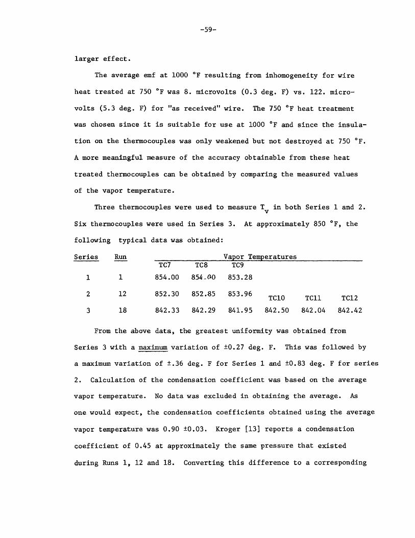
-59-

larger effect.

The average emf at 1000 *F resulting from inhomogeneity for wire

heat treated at 750 *F was 8. microvolts (0.3 deg. F) vs. 122. micro-

volts (5.3 deg. F) for "as received" wire. The 750 *F heat treatment

was chosen since it is suitable for use at 1000 *F and since the insula-

tion on the thermocouples was only weakened but not destroyed at 750 *F.

A more meaningful measure of the accuracy obtainable from these heat

treated thermocouples can be obtained by comparing the measured values

of the vapor temperature.

Three thermocouples were used to measure Tv in both Series 1 and 2.

Six thermocouples were used in Series 3. At approximately 850 *F, the

following typical data was obtained:

Series Run Vapor TemperaturesTC7 TC8 TC9

1 1 854.00 854-00 853.28

2 12 852.30 852.85 853.96 TC10 TC11 TC12

3 18 842.33 842.29 841.95 842.50 842.04 842.42

From the above data, the greatest uniformity was obtained from

Series 3 with a maximum variation of ±0.27 deg. F. This was followed by

a maximum variation of ±.36 deg. F for Series 1 and ±0.83 deg. F for series

2. Calculation of the condensation coefficient was based on the average

vapor temperature. No data was excluded in obtaining the average. As

one would expect, the condensation coefficients obtained using the average

vapor temperature was 0.90 ±0.03. Kroger [13) reports a condensation

coefficient of 0.45 at approximately the same pressure that existed

during Runs 1, 12 and 18. Converting this difference to a corresponding

Urn,.IIW I Wau

-60-

temperature, the average vapor temperature reported for Runs 1, 12 and

18 would have to be in error by approximately 4. deg. F to account for

the difference.

It is the author's opinion that Series 2 thermocouples did not

receive a complete heat treatment. Whereas the insulation on wires

from Series 1 and 3 was uniformly white after the heat treatment, the

insulation on wires for Series 2 was not. The exposure time in the

furnace was increased to 1-1/2 hours for Series 3.

Extra thermocouples were heat treated and sent to Conax Corporation

for calibration. The resulting correction was of the order of 7 deg. F

at 850 *F. Since this correction was to be applied to all thermocouples,

it had a small effect on the calculated value of the condensation

coefficient; however, the correction was included for completeness.

-61-

APPENDIX D

Simplified Derivation of Temperature Distribution at Wall

In the body of this thesis, the distribution of possible wall

temperature measurements for the condensing block is presented assuming

a Gaussian distribution of temperature measurements at each thermocouple

hole. To demonstrate the steps required to obtain the wall temperature

distribution, the following solution was derived for a condensing block

with two holes. A cosine function, with its finite limits, was assumed

for the distribution of possible temperature measurements in each hole.

The cosine function was chosen because it is easier to handle than the

Gaussian function.

Equation for Tw as a function of (Tl, T2, '1, '2)

AT

'Tw

HOLE #1T

HOLE #2

T 2

xy x 2

Knowing that the equation for the line shown must be of the form

T = Tw + mx, one can solve for Tw

T = T x 2 - 2 x1 (D-1)w x2 ~ 1

MIMMIIWII 10 "1111

-62-

Density Function of Possible Errors in Hole #1

By assuming both a linear temperature drop across hole #1 and a

cosine density function for the temperature readings at hole #1, one

obtains the density function f1 (T1 ) as given by (D-2). This density

function will also be referred to as the marginal density function of

T The limits were obtained by applying the well known Fourier Equation

with T equal to the undisturbed temperature at the centerline of hole

#1. r( if (T1) = Cos L I (D-2)

1 1 4( A)(R)r 2( -)r

k . k .

- )r 0 ( )r

Marginal Density Function of Possible Error at Wall

Setting x1 and x2 equal to the known locations of the hole center-

lines, the density function f3 (Tw) is obtained by using the approach

of [29]. With x1 and x2 as constants and T1 and T2 as independent

variates with known marginal density functions, one imagines T2 to be

(q/A)r - (/~held fixed while T varies from T - k to T + k .The

conditional probability of Tw given T2, #(Tw I T2), is given by:

(T IT2 f1 (1 (D-3)w

From (D-1): Tw (x2 - x1+ T2 1 (D-4)1 2

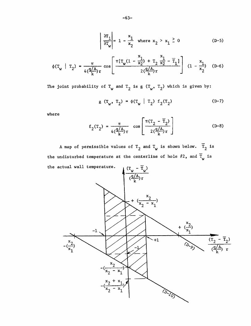
MllgiIhIIIMII, I~hl~i IIN n Ila ,

-63-

aT ~x11 11 where x >x 0

w 22 1

xl1 xl 1

[Tw(1 - ) + T2 2 11

) [(q[Tlr 2 (gIA) r -Tk -/ k

1

(1 )x2

The joint probability of Tw and T2 is g (Tw, T2) which is given by:

g (Tw, T2) = $(Tw I T2 f2 (T2)

where

(D-5)

(D-6)

(D-7)

f (T ) = /Ak )r

Tr(T2 - T2)cos 22( k)r

A map of permissible values of T2 and Tw is shown below.

the undisturbed temperature at the centerline of hole #2, and Tw is

the actual wall temperature.

-l.

X2

2

x

+1x 2x-

x 2 + x1

X2 1

#(T w I T 2)

(D-8)

T2 is

T2 )

-64-

(T -Tw 2 1 2 2)=I -x ( ) g (D-9)

( )r 2 1 2 1 ( )rk k

(Tw Tw 2 1 2 - T2)

( )r 2 1 x2 1 (Ck)rk k

(D-9) was obtained by inserting the maximum permissible value of

T, namely Y + (VA )r, in (D-1) and noting that T = T )1'1 k 1 w k 1

and that T2 w A) x2 . Likewise, (D-10) represents the minimum

Yl- (_q/ A)permissible value of TI, namely - k.

To obtain the marginal density function f3 (Tw), one integrates

the joint density function g(Tw, T2) with respect to T2 '

(T max.

f3 (T ) = g(Tw, T2) dT2 (D-ll)

(T2 ) min.

As can be seen from the previous map of permissible values of

T2 and T , f3 (T ) can be obtained by performing two integrations and

recognizing that f3 (Tw) must be symmetrical about T Yw

For the following range of (Tw - T )

2 +x)(/A)r (T -T) - ( )rx2 ~ 1 k w w k

the limits on the integration are

(,/r x2 x2 ~ xl T - T (T T) - + (A)rk /x 1 x w w 2 2 k

and the results of the integration yield:

-65-

f (T ) = [-7cos { + w3 w 8r (k )(1 + ) 2 x 2 /Ar x2

(D-12)

1 T "2 w - w 1l-- - cos (WW)(1 )x ___s2x /Af

2 2 x1 k r 12.. k

For the following range of (Tw - Tw)

-A r '_' (Tw ~ w 0

k w w

the limits on the integration are

- (/A)r < (T - T2 ) +( )rk 2 2 k

and the results of the integration yield:

f (T ) = cos ( ) cos T (1 1)(w_-T (D-13)3 w ___ l j x 1 2 x 2 x 2 q/A r

4r(k)(1 + )k2

It is very interesting to note that wherever Tw appears in (D-12)T -T

and (D-13) it appears as part of the dimensionless group ( w

krThis same group results from the analysis used in the body of this

thesis. The following figures show the marginal density function

assumed at hole #1 and the resulting marginal density function at the

wall. Both are plotted using dimensionless groups. Simply by multi-

plying (D-12) and (D-13) by ( r), these equations were converted

from a function of the variable T to a function of the variableT -T ww w

(/A rkr

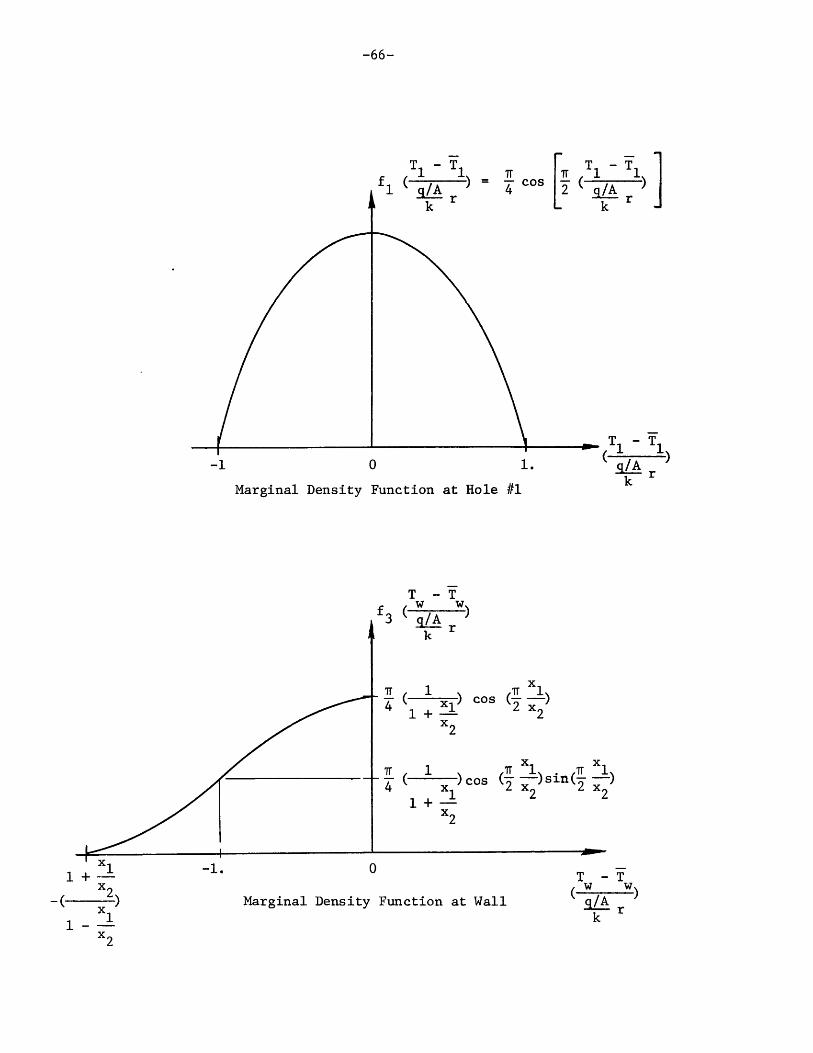
-66-

T - TT

1 /A r 4 2k r

T -T

q/A rk

-1 0 1.

Marginal Density Function at Hole #1

T T

k rk

T -Tf w wy

k

7r 1 7 1) Cos( )

1 +- 22x2

- ( 1 )co ( )sin(-1 x+ 2 x 2 x2

+x2

+, xl0

Marginal Density Function at Wall

T -Tw w

g/A rk

- 2-)

x2

-67-

From the previous limits, one gets:

T -T 1+w W x2 (D-14)q/A rxik max. x2

From (D-2), one gets:

Ty - T1 1 (D-15)

r/A rk max.

x1Unless (-) = o, the maximum error in temperature measurement at

x2

the wall is greater than that assumed in a hole at x1 or x2. It follows

that the first thermocouple hole should be as close to the wall as pos-

sible (x1 + 0) and that the last thermocouple hole should be as far

from the wall as possible (x2 -+ c). By rewriting (D-14) as follows,

the powerful effects of material conductivity and hole .Ladius are seen.x.I

T -Tw w 2_ _ (D-16)qIA max. 1

2

For example, simply by converting to copper (k = 210) from stainless

steel (k = 12), one can reduce the possible error in the wall tempera-

ture measurement by 1650. %.

Knowing the marginal density function at the wall, one can obtain

any statistical parameters of interest. If one had been concerned only

with the standard deviation at the wall, this could have been obtained

for this linear case without calculating f3 (T ).

Standard Deviation at the Wall

For the linear case, it is easier to obtain the standard deviation

-68-

at the wall indirectly by obtaining the standard deviation in a hole

and then applying the formula for the variance of a linear function

than to obtain it directly by making the necessary integrations usingT1 - T1

(D-12) and (D-13). The variance of ( 1 ) is obtained as follows:krk

1 12T1 - T Tf T, T T, T,- T,

Variance of TiJ= - [ T/ j cos - /A -lJ d =/A J 0.19

-k -1 - k _ k k

By rewriting (D-1) as follows:

T -] x2 Tl - T x TT2 1

_r 2 1 r 2 1 / r- k - k J k

the variance at the wall is easily obtained using the formula for the

variance of a linear function [29]. This yields:

T - Ti xF

Variance of r 2 2 (Variance 1[ /A r [x 2 x1j Hole 1k

+ ( (VarianceHole 2x2 x1 Hl

xl1 + (-)

x2= 2 (0.19)

(1 -)x2 21x2 xTw- 1+ (r)

The standard deviation off q/A x (0.436) (D-17)

L wj (1--)x2

This result could have been obtained using Eq. (7) from the main

body of this thesis with S = 0.436. To apply (D-17) to a condensing

block with more than two holes, set x1 of (D-17) equal to x min. for the

-69-

block of interest and set x2 = x . Using the information tabulated2max.

in Section 7.4 of the body of the thesis, (D-17) was evaluated for the

present system and the systems of [12] and [13]. Once again, the

"effective radius", which is equal to twice the actual radius, was

used to correct for the distortion of isotherms around the hole. The

results from (D-17) are compared to the complete results as given in

the body of the thesis in the following table. As shown in the table,

(D-17) is an excellent approximation to the complete result and is an

acceptable estimate of the possible experimental error in wall tempera-

ture measurement.

System

Wilcox

Kroger [13]

Meyrial [12]

T -T

q/A )at 1 St. Dev.

2 Hole Result All Hole Result(D-17) (Eq. 7)

9-1 x 10-6 *F/(BTU/hr ft 2) 4.8 x 10-6

9.2 x 10-5 5.8 x 10-5

2.4 x 10~4 1.6 x 10~4

-70-

APPENDIX E

Additional Analysis of Error

From experiment, the temperature of the cold wall (T ), the tempera-

ture of the saturated vapor far from the condensate (TV), and the heat

flux (q/A) are determined. From these measured quantities, the tempera-

ture at the free surface of the condensate (T ) and the condensation

coefficient (a) are calculated. It has been stated that Tw, which is

measured by extrapolation, is generally subject to the greatest experi-

mental error. Since measured temperature differences (Tv - T w) are very

small, errors in Tw have a large effect on the calculated condensation

coefficient.

Error in Vapor Temperature Measurement Due to Fin Effect

It obviously follows ,hat errors in Tv also have a large effect

on the calculated condensation coefficient. Since Tv was measured by

inserting a thermocouple into a well which protruded into the vapor,

the recorded Tv is actually the temperature of the far end of the well.

To compare the temperature at the far end of the well with the tempera-

ture of the vapor, the thermocouple well can be modeled as a pin fin

protruding from a surface. Neglecting the heat transfer from the end

of the fin, [30] gives the following relation between the pertinent

variables:

T - Tv v 1T - T cosh(mk)w.w. v

where Tv = measured temperature from thermocouple in the well

Tv = actual vapor temperature

-71-

T wow = temperature of wall at

m2 = (h' P') / (k' A')

h' = heat transfer coefficient

P' = perimeter of well

k' = conductivity of well

A' = cross-sectional area of we

k = length of well

base of thermocouple well

between vapor and well

Thermocouples were spot welded to the outside surface of the loop.

These thermocouples were located at the base of thermocouple wells which

were used to measure the vapor temperature. From these readings,

(T - T ) < 2 deg. F. For this case (E-1) can therefore bev w.w. max.

written as follows:

(T - T )'y vimax< 2

cosh(mk) - 1

Since no auxiliary heaters were present in the test section, con-

densation did take place on the stainless steel wells and, therefore,

the applicable h' is that associated with condensation (h' % 20,000

BTU/hr ft2 *F). Applying (E-2) to the thermocouple wells used in the

measurement of the vapor temperature, one obtains a measure of the

error (T - T ) associated with the fin effect:v v

Stainless Steel Thermocouple Wells

3/16 0.D. x 0.042 wall x 1.6 inches

3/32 0.D. x 0.020 wall x 4.0 inches

(T v- T v) deg. Fv v

10-43

10-162

One obviously concludes that the ends of both thermocouple wells

are at the actual vapor temperature. This is consistent with the fact

(E-2)

-72-

that measured vapor temperatures from the two designs are the same.

For the work reported in this thesis, the error in the vapor temperature

measurement due to the "fin effect" is completely negligible.

If the walls of the test section had been heated with auxiliary

heaters to a temperature above Tv, the applicable h' to use in (E-1)

would not have been that associated with condensation. The applicable

h' would have been 02. BTU/hr ft2 *F. Using (E-1), a significant wall

temperature influence would have been calculated, and a meaningful

difference would exist between the two designs.

(q/A) Error - Condensing Block

The actual temperature profile in the block in terms of the

formulation of Eq. (7) is:

T -T -V.x

q/A r rk

-lwhere the slope is (-). A distribution of "measured slopes" will resultr

from the uncertainty of the temperature measured in a hole as described

in Section 7.3. Analysis of the distribution of possible measured

slopes resulting from this uncertainty yields, according to [21], that

the standard deviation of the slope =

SnZ (x - y)2

i=1

where y&=- E x.n. i

x = distance of "i" the hole from wall

n = number of holes

S = standard deviation of distribution in hole.

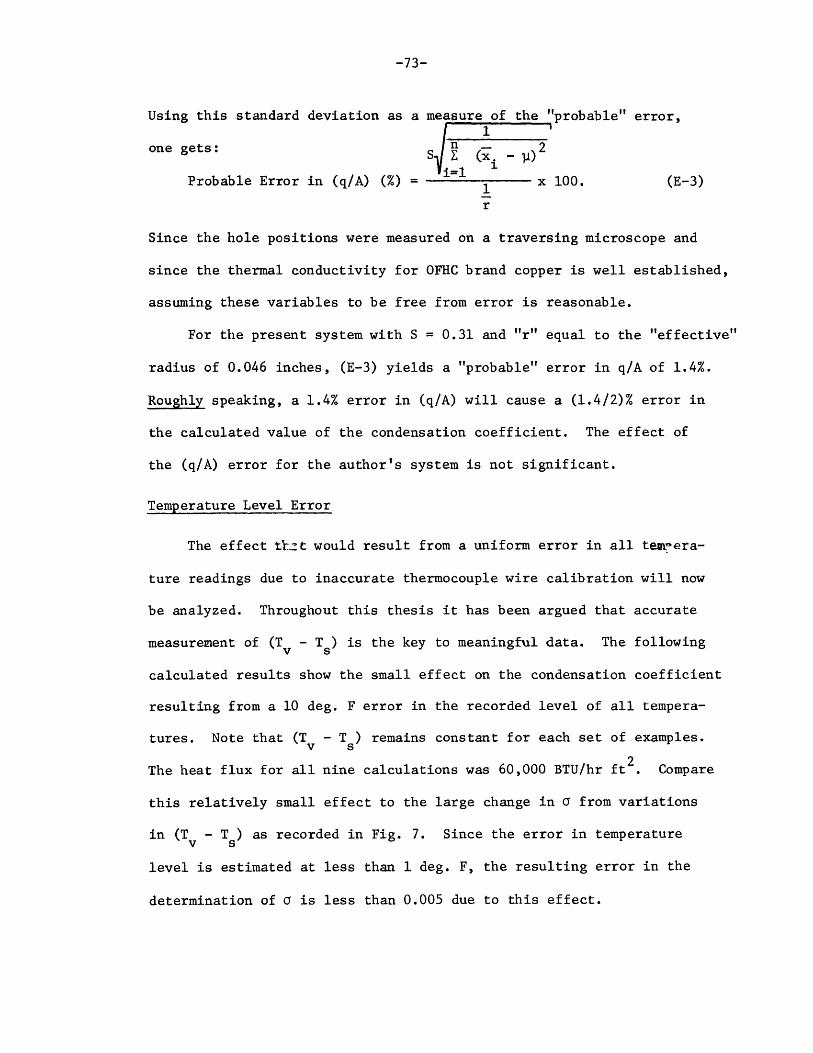
-73-

Using this standard deviation as a measure of the "probable" error,

one gets: - 2S (x. Wi=1

Probable Error in (q/A) (%) = x 100. (E-3)

r

Since the hole positions were measured on a traversing microscope and

since the thermal conductivity for OFHC brand copper is well established,

assuming these variables to be free from error is reasonable.

For the present system with S = 0.31 and "r" equal to the "effective"

radius of 0.046 inches, (E-3) yields a "probable" error in q/A of 1.4%.

Roughly speaking, a 1.4% error in (q/A) will cause a (1.4/2)% error in

the calculated value of the condensation coefficient. The effect of

the (q/A) error for the author's system is not significant.

Temperature Level Error

The effect thzt would result from a uniform error in all temwera-

ture readings due to inaccurate thermocouple wire calibration will now

be analyzed. Throughout this thesis it has been argued that accurate

measurement of (T - T ) is the key to meaningful data. The followingv S

calculated results show the small effect on the condensation coefficient

resulting from a 10 deg. F error in the recorded level of all tempera-

tures. Note that (T - T ) remains constant for each set of examples.v s

2The heat flux for all nine calculations was 60,000 BTU/hr ft2. Compare

this relatively small effect to the large change in a from variations

in (T - T ) as recorded in Fig. 7. Since the error in temperaturev s

level is estimated at less than 1 deg. F, the resulting error in the

determination of a is less than 0.005 due to this effect.

MkI IMMlu.",,

-74-

T (*F) T (*F) (T -T) a

740.00 733.47 6.53 1.05

750.00 743.47 6.53 1.00

760.00 753.47 6.53 0.95

890.00 888.32 1.68 1.04

900.00 898.32 1.68 1.00

910.00 908.32 1.68 0.96

1140.00 1139.67 0.33 1.03

1150.00 1149.67 0.33 1.00

1160.00 1159.67 0.33 0.97

Nusselt Analysis-Errors

As can be seen from Fig. 11, the resistance of the liquid film

is small compared to the interphase resistance except at the highest

pressure (0.15 atm.) considered in the author's experiments. At 0.15

atm., the two resistances are equivalent. It follows that minor in-

accuracies in the Nusselt analysis will have a very small effect when

the Nusselt resistance is small compared to the interphase resistance.

Minor modifications of the Nusselt analysis are possible. For example,

the effect of momentum and shear stress evaluated according to [3]

would increase the resistance of the film by mi%. Although this and

other modifications are possible, the greatest uncertainty appears to

be the correct boundary condition to apply at the top of the condensing

surface. The Nusselt analysis assumes the film thickness to be zero at

the top of the condensing surface. Since in the present equipment

-75-

condensation does take place on the walls, the film thickness is not

zero at the top of the condensing surface. To avoid having such inac-

curacies in the film analysis seriously affect the calculated condensa-

tion coefficient, experiments were curtailed at 0.15 atm.

Effect of Variation of T on the Condensation CoefficientV

As is discussed in Appendix C, there was some variation in the

individual vapor temperature readings for each "Run". The magnitude

of this variation, which is probably due primarily to the remaining

inhomogeneity of the thermocouple wire, seemed to depend on the effective-

ness of the heat treatment given to the wires. New thermocouples were

fabricated, heat treated and installed for each of the three Series

which were run. To show the effect of these variations in Tv, a was

calculated using the individual readings of T . The temperature atv

the surface of the liquid film obtained for the Run-was used in the

calculations. Figures El, E2, and E3 show the results from these cal-

culations and the result obtained using the average T.. The "circled"

points in the figures are individual data points, and the "slash"

represents the average vapor temperature for the Run. The average vapor

temperature was used in the results reported in the body of the thesis.

The three figures refer to the three Series which were run.

The sensitivity to accurate determination of T or (T - T ) isv v S

very evident in the figures. To obtain high confidence in experimental

data, one should use the average from a number of thermocouples which

measure T . In addition, one should have the ability to replace all

thermocouples between Series. The variations in a shown in Fig. E-2

cause little concern because the averaged results agree with the higher

- - inEImErnmI~Iim.ii.rn

-76-

precision results shown in Fig. El and E3. Three thermocouple wells

were used to measure T for Series #1 and #2. Three additional wells

were installed after Series #2, and therefore six values of T were

obtained in Series #3. The resulting a obtained using the average T

agree for all three Series.

General Comment on Error

Of all errors, those associated with the measurement of Tw are,

in general, predominate. For the author's system, the uncertainty due

to the effect of inhomogeneities in the thermocouples is of the same

order of magnitude as the uncertainty in the wall temperature measure-

ment (neglecting inhomogeneity). For others who used nickel or stainless

steel condensing blocks, the lack of precision in the measurement of Tw

dwarfs the inhomogeneity effect; therefore, the effect of inhomogeneity

was not discussed in general in the body of the thesis.

-77-

APPENDIX F

Additional Information on Effect of Second Condenser

The second condenser (Fig. 2) was used as described in the main

body of this thesis to determine whether non-condensable gas was ac-

cumulating at the test condenser and significantly affecting the experi-

mental data. In addition to the data taken at 'V0.02 atm. (Fig. 18),

data were also taken at 00.06 atm. (Fig. Fl). Note in Fig. Fl that as

the heat extracted at the second condenser increased, the condensation

coefficient increased from %0.86 to 10.96. For the "Runs" shown this

corresponds to a change in (T - T ) of less than 0.25 deg. F. SinceV S

the effect shown in Fig. Fl is small and since no effect is shown in

Fig. 18, it is simply concluded that the effect of non-condensable gas

in these experiments was not significant.

110111111911,

-78-

APPENDIX G

Listing of Coaluter Programs

-79-

PAGE 2 DATA ANALYSIS PROGRAM NO. 1 (WILCOX)

THIS PROGRAM WRITTEN TO PERFORM THE FOLLOWING JOBSCONVERT MILLIVOLT TC OUTPUT TO DEGREE FMAKE LEAST SQUARES FIT STRAIGHT LINE OF TEMP IN BLOCK.COMPUTE HEAT FLUX, SURFACE TEMPtHEAT TRANS COEFF.

REAL MVLT(40)DIMENSION DEV(40DIMENSION Y(40)IR=2IW=3

).POTC(40) TMP(40),DATA(40) CALB(40) DIST(40)

C DATA INPUT

READ(IR#91) NOPTNO91 FORMAT(212)

DO 10 I=loNOPT10 DIST(I)=O.

READ(IR99) (DIST(I)91=1NO)5 READ(IR99) (MVLT(I),1=1NOPT)9 FORMAT (7F10.0)

IF(MVLT(1)) 99,99988 CONTINUE

C CONVERSION OF MILLIVOLT TC OUTPUT TO DEGREE F

DO 15 Iz1gNOPTDATA(I)=MVLT(I)MUNITuMVLT(I)/10.VLTz(MVLT(I)/10.)-MUNITCORFs-0.101E- 02+0.100E- 01*VLT-O.272E- 03*VLT**21 +0.315E-03*VLT**3-0.126E- 03*VLT**4

C POTC IS CORRECTION FOR SLIDE WIRE CALIBRATION ON POTENTIONMETERPOTC(I)=CORF*10.MVLT(I)=(MVLT:I)/10. + CORF)*10.TMP(I)= 55.40606 + 42.55409*MVLT(I) -0.00515*(MVLT(I)**2.)

C NEXT CARD CORRECTS FOR CALIBRATION OF WIRECALB(I)= -1.*(1.7768594 + 0.0063321*TMP(I)TMP(I)=TMP(I) + CALB(I)

15 CONTINUE

C LEAST SQUARES FIT OF STRAIGHT LINE TEMP GRADIENT

DO 18 I=lsNOPT18 Y(I)=TMP(I)

CALL JSHLS(NO#DIST#Y#POIN#SLEP)DO 20 I=19NOPTDEV(I) = TMP(I) - (POIN + SLEP*DIST(I))

20 CONTINUE

C COMPUTAYION OF HEAT FLUX. SURFACE TEMPtHEAT TRANS COEFF

DATA ANALYSIS PROGRAM NO. 1 (WILCOX)

COND=230.42105 - 0.026316*TMP(3)HTFX= -12.*COND*SLEP

C CALCULATES TWALL AND TSAS(SURFACE TEMPERATURE)XNCON=(211. + 0.1534*POIN )/12.TWALL= POIN - SLEP*0.0017*COND/XNCONDENL=52.1666 - 0.007666*TWALLDENVA=2.71828**(.00768*TWALL-13.82)VISL=0.80197 - O.0003733*TWALLCONDL= 29.2094 - O.008066*TWALLCPLW0. 183XLEN=0.0825HFG=991.2854-0.101428*TWALLTSAS=TWALL+((HTFX /0.943)**1.333)*((XLEN*VIS1(DENL-DENVA)*(CONDL**3.)*HFG))**.333)HFGC=HFG+CPLW*(TSAS-TWALL)*0*375TSAS=TWALL+((HTFX /0.943)**1.333)*((XLEN*VIS1(DENL-DENVA)*(CONDL**3.)*HFGC))**.333)DTMP= TMP(NO + 1) - TWALLHTC=HTFX/DTMP

L/(DENL*4.17312E8*

L/(DENL*4.17312E8*

C DATA OUTPUT

WRITE(IW933) HTFX9DTMP9HTC33 FORMAT (lHl940X'RUN NO ' //

1F4.291OX'HEAT TRANS COEFF='#F92X'DATA' 7X'CORRECTION'3X'IMILL3 DEVIATION')DO 31 I=1NOPT

31 WRITE(IW,34) IgDIST(I)*DATA(I)ii)

10X'HEAT FLUX=.1 // 1X'POSITIVOLT' 8X'CALB

I PF9.110XION NO'.5X(F) '.3X'

TEMP DIF=DISTANCE'TEMP(F)

OPOTC(I) .MVLT(I),CALB(I),TMP(I) DEV(

34 FORMAT(I7,1F16.4,3(7X,1F7.3) 6X.F8.2,6X,F8.2,6XF8.2)WRITE(IW#35) SLEP#POIN

35 FORMAT (//10X'TEMP = ',F8.29' X DIST + ',F8.2)WRITE(IW936) TWALL#XNCONtCOND

36 FORMAT(/10X'TWALL= ',F8.2,10X'INICKEL CONDUCTIVITY=',F8.2,10X'COPPE1R CONDUCTIVITY='.F8.2)WRITE(IW#37) TSAS ,DENVADENLCONDLVISL,HFGHFGCCPLW

37 FORMAT(/10X'TSAS='FB.2lOX'VAPOR DENSITY=',F8.5,1OX'LIQUID DENSITlYz 'tF8.29//10X'CONDUCTIVITY LIQUID=',F5.2,31X'VISCOSITY LIQUID=',2F5.3,//10X'HFG=',F8.2,12X'HFG+CP EFFECT=',F8.2,10X'CP LIQUID=',F8.35)GO TO 5

99 CALL EXITEND

FEATURES SUPPORTEDIOCS

PAGE 3

-80-

-81-

PAGE 2 DATA ANALYSIS PROGRAM NO. 2 (WILCOX)

C THIS PROGRAM WRITTEN TO PERFORM THE FOLLOWING JOBSC CALCULATE CONDENSATION COEFFICIENT USING PSAV AND PSASC AND ALSO CALCULATE A 'COEFFICIENT' USING PSAI AND PSAS.

C TSAV=TEMP. OF SAT. VAPOR AT 'V'(F)--PSAV=ABS. PRES. OF SAT. VAPOR AT 'V'(ATM)C TSAI=TEMP. OF SAT. VAPOR AT *I'(F)--PSAI=ABS. PRES. OF SAT. VAPOR AT 'I'(ATM)C TSAS=TEMP. OF SAT. VAPOR AT 'S'(F)--PSAS=ABS. PRES. OF SAT. VAPOR AT 'S'(ATM)C CONDQ=BTU/(HR FT**2) CONDW=LBM/(HR FT**2) HFG=BTU/LBMC CPSAV=BTU/(LBM F) VSAV=LBM/(FT HR) XKSAV=BTU/(HR FT F)C GSAI=DIMENSIONLESS XMSAI=MOLECULAR WEIGHT AT IC PATH=PATH LENGTH AT 'I' IN CENTIMETERS DFET AND DTHEO ARE IN CENTIMETERSC SIGMA-KROG=SIGMA CALCULATED WITH PV AND PS.C SIGMA=SIGMA CALCULATED WITH PI AND PS.C ALL VAPOR PROPERTIES ARE FROM WEATHERFORD. PATH IS FROM HIRSCHFELDER.

IR=2. 1130IW=3. 1130

9 READ(IR910) TSASTSAVCONDQRUN10 FORMAT(4F10.3)

IF(TSAV) 898,898,1111 CONTINUE

PSAS=10O.**(4.185-(7797.6/(TSAS+460.))) KPSAV=10.**(4.185-(7797.6/(TSAV+460.))) KCPSAV=0.01463061+O.0002701871*TSAV-8.979*TSAV*TSAV*(1.E-8) K

XKSAV=0.00457429 + (0.00000252857*TSAV) KXMSAV=37.00084+0.003154*TSAV KVSAV=0.0261286 + (0.0000148571*TSAV) KHFG=991.2854-0.101428*TSAV KCONDW=CONDQ/HFGSIGMA=(8.527009E5)*(PSAV-PSAS)*((XMSAV/(TSAV+460.))**0.5)/CONDW 1 OF 2SIGMA=2./(1.+SIGMA)DPVSS=(PSAV-PSAS)/PSASWRITE(IW,19)

19 FORMAT(///,' RUN TSAV TSAS CONDO')WRITE(IW,20) RUNTSAVTSASsCONDO

20 FORMAT(lF5.0,2F10.3,1F10.1,/)WRITE(IW,21)

21 FORMAT(9X,4HPSAV,6X,4HPSAS.6X.5HCPSAV,5X.4HVSAV96X95HXKSAV,4X,3HHF1G,6X,5HCONDW,4X,1OHSIGMA-KROG,3X,5HDPVSS)WRITE(IW,22) PSAVPSASCPSAVVSAVXKSAVHFGCONDWSIGMADPVSS

22 FORMAT(5X,5F10.5,1F1O.2.3F10.5,//)

C IF DATA SWITCH 1 IS UP. THE PROGRAM ALSO CALCULATES USING PSAI AND PSAS.C XN= NUMBER OF PATH LENGTHS IN TEMPERATURE JUMP EQUATION.

XN=10.TSAI=TSASCALL DATSW(1,IEXIT)IF(IEXIT-1.5)1029102,9

102 CONTINUECPSAI=0.01463061+0.0002701871*TSAI-8.979*TSAI*TSAI*(1.E-8) K

Im~ililliki

-82-

PAGE 3 DATA ANALYSIS PROGRAM NO. 2 (WILCOX)

XKSAI=0.00457429+ (0.00000252857*TSAI)PSAI=l0.**(4.185-(7797.6/(TSAI+460.)))XMSAI=37.00084+0.003154*TSAIVSAIO.0261286+ (0.0000148571*TSAI)GSAI=l.718142-0.00007571&*TSAIXNOMOa(1.320497E22)*(PSAI)/(TSAI+460.)AMOL=((1.51000E-18)*(XMSAI*(TSAI+460.))**o.5)/VSAIPATH=0.707/(AMOL*XNOMO)DFET=XN*PATHDTHEO=2.*GSAI*PATH*XKSAI/(CPSAI*VSAI*(GSAI+1.))TI=CONDW*CPSAI*(DTHEO+DFET)*(O.03281)/XKSAITI=(TSAV)*(1./(1.+(1./TI)))+(TSAS)*(1./(1.+TI))IF( ABS(TI - TSAI) - 0.01)300,200,200

200 TSAI=TIGO TO 102

300 TSAI=TISIGMAS(8.527009E5)*(PSAI-PSAS)*((XMSAI/(TSAI+460.))**0.5)/CONDWSIGMA=2./(1.+SIGMA)DPISS=(PSAI-PSAS)/PSASWRITE(IW,30)

30 FORMAT(' XN SIGMA TSAI PSAI DFET DTHEO1 PATH DPISS')WRITE(IW,31) XNSIGMA.TSAIPSAI DFET.DTHEO,PATHDPISS

31 FORMAT(lF5.le2F10.3.1F1O.5.3F10.6.1F1O.5,/)WRITE(IW,32)

32 FORMAT(10X,5HCPSAI,4X,4HVSAI,6X,5HXKSAI,5X,4HGSAI,5X,5HXMSAI)WRITE(IW,33) CPSAIVSAIXKSAIGSAIXMSAI

33 FORMAT(5X,5F10.5,//)GO TO 9

898 CALL EXITEND

FEATURES SUPPORTEDIOCS

TIME USED- 3 TIME LEFT-

KKKKK

1 OF 22 OF 2

1 OF 22 OF 2

LOGGED OUT 387 LOGIN- 8

-83-

PAGE 2 CALCULATION OF EXPECTED VALUE OF SIGMA

CALCULATION PERFORMED FORDATA REQD.--RADIUS OF HOLEDIMENSION F(35)IR=2.IW=3.READ(IR96) (F(I)tIul932)FORMAT(7F10.0)READ(IR98) R#SDFORMAT(7F10.3)IF(R) 900,900.9

9 CONTINUEXLEN=0.0825CPLW0. 183TSAV=550.WRITE(IW913)

13 FORMAT(lH14X'TSAV10*(C) FXEE FXFF FXGG

K=129 289 210.AND DIMENSIONLESS STD.

PSAVTE

(TV-TS)/Q/ATF

DEV. AT WALL.

D 12*(C) 28*(C) 21TG SIGME SIGMF SIGMG')

50 TSAV=TSAV+50.PSAV=10.**(4.185-(7797.6/(XMSAV=37.00084+0*003154*TSAHFGa991.2854-0.101428*TSAVDENL=52.1666 - 0.007666*TSADENVAa2*71828**(.00768*TSAVVISL=0.80197 - 0.0003733*TSCONDL= 29.2094 - 0.008066*T

'DO IS NUSSULT RESISTANCE.CLAUSIUS CLAPERON EQUATIONONLY 'C' (NOT D) IS USED TO

'I

US0

TSAV+460.)))V

V13.82)

AVSAV

C' IS INTERPHASE RESISTANCE.ED TO OBTAIN FORMAT OF 'C'.BTAIN EXPECTED VALUE OF SIGMA.

Du(1./O.943)*((XLEN*VISL/(DENL*4.17312E8*(DENL-DENVA)*(CONDL**3.)*1HFG))**.25)Cu(1.986*(TSAV+460.)*(TSAV+460.)*SQRTU(TSAV+460.)/(XMSAV)))/(HFG*H1FG*PSAV*8.527009E5*XMSAV)

E=12.*(C)FFFF=28.*(C)Gu210.*(C)HuSD*(R/12.)EE=E/HFF=FFFF/HGG=G/H

C CALCULATIONS FOR K=12.IF(EE-3.1) 20921.21

20 N=EE*10.+1.FXEExF(N) + (F(N+1)GO TO 22

(STAINLESS STEEL)

- F(N))*((EE*10. + 1.)-N)

CC

678

-84-

PAGE 3 CALCULATION OF EXPECTED VALUE OF

FXEE=1.RTEE=O*5*FXEENO0.

23 NzN+1.IF(RTEE-(1.-F(N))) 23.23,24

24 TE= (((N-1.)/10.) - 0.1*((RTEE+F(N)SEuTE/12.SIGME=2./((SE/C)+2.)

C CALCULATIONS FOR K=2IF(FF-3.1) 30.31,3

?0 N=FF*10.+1.FXFFaF(N)+(F(N+1)

3132

GO TO 32FXFF..RTFF=0.5*FXFFNz0.

8. (NICKEL)1

-F(N))*((FF*10.+1.)-N)

33 N=N+1.IF(RTFF-(1.-F(N))) 33,33,34

34 TF= (((N-1.)/10.) - 0.l*((RTFF+F(N)SF=TF/28.SIGMF=2./((SF/C)+2.)

C CALCULATIONSIFIGG-3.1)

40 N=GG*10.+1.

FO40

FXGG=F(N) +GO TO 42FXGG=1.RTGG=0.5*FXGG

R K=210.941,41

F(N+1)

(COPPER)

-w F(N))*((GG*10.+1.)-N)

N=0.43 NuN+1.

IF(RTGG-(1.-F(N))) 43,43,4444 TG= (((N-1.)/10.) - 0.l*((RTGG+F(N)

SG=TG/210.SIGMG=2./((SG/C)+2.)

WRITE(IW,14)1SIGMFoSIGMG

-1.)/(F(N)-F(N-1))))*H

TSAVPSAV.CDEFFFFGFXEEFXFFFXGGTETFTGSIGME,

14 FORMAT(3XF7.2,F8.5,2F10.7,3F8.5,3F5.2,3F8.5,3F6.3)IF(1400.-TSAV) 800,50,50

800 WRITE(IW,12) SDtR.HtXLEN12 FORMAT(//3X'ST. DEV. INPUT =',F9.7,3X'RADIUS OF HOLE=',F5.3,'INCHE

iS STD DEV FOR SURFACE=',F8.6,'FEET LENGTH=',F6.4,'FEET')GO TO 7

900 CALL EXITEND

FEATURES SUPPORTED

2122

SIGMA

4142

-1.)/(F(N)-F(N-1))))*H

-le)/(F(N)-F(N-1))))*H

-85-

Values of F(I) for "Calculation of Expected Value of Sigma" are

as follows:

() F(I) (I) F(I)

1 .5000 17 .9452

2 .5398 18 .9554

3 .5793 19 .9641

4 .6179 20 .9713

5 .6554 21 .9772

6 .6915 22 .9821

7 .7257 23 .9861

8 .7580 24 .9893

9 .7881 25 .9918

10 .8159 26 .9938

11 .841' 27 .9953

12 .8643 28 .9965

13 .8849 29 .9974

14 .9032 30 .9981

15 .9192 31 .9987

16 .9332 32 1.0000

-86-

PAGE 2 THIS SUBROUTINE FITS A FIRST ORDER CURVE

SUBROUTINE JSHLSDIMENSION X(1),

C SET SUMS TO ZEROYY=0.OXX=0.0XY=0.0X2=0.0

C FORM SUMSDO 1 IzleNXX=XX +X(I)YY=YY+ Y(I)XY=XY+X(I)*Y(I)X2=X2+ X(I)**2

1 CONTINUEC SETUP THE INPUT

AA(1)=YYAA(2)=XYBB(191)=NBB( 1,2) =XXBB(2,1)=XXBB( 2,2) =X2

C SOLVE MATRIXC SIMQ IS A IBM SC

CALL SIMQ(BB#AA9A=AA(1)S=AA(2)RETURNEND

NtXYAB)1) ,AA(2) BB(292)

FOR SIMQ

IEN.SUB.29K)

PACKAGE WHICH SOLVES SIM. LIN. EQS.

-87-

APPENDIX H

Theoretical Effect of Non-Condensable Gas on the Condensation Coefficient

It is shown in this appendix that the pressure dependence of the

condensation coefficient reported by some investigators cannot be ex-

plained as due to non-condensable gas. The effect of a constant mass

of non-condensable gas in a system is shown to reduce the measured con-

densation coefficient (a) to a value which is dependent only on the mass

of gas present and on the molecular properties of the diffusing gases.

The effect on the measured condensation coefficient is independent of

vapor pressure and heat flux!

The analysis requires the following steps:

a) Obtain an expression for the partial pressure of the non-

condensable gas.

b) Assuming that the actual condensation is unity (as would be

measured when no non-condensable gas is present), obtain an

expression for the measured condensation coefficient including

the effect of the partial pressure of the non-condensable gas.

c) Combine results from (a) and (b) to obtain the effect of non-

condensable gas on the measured condensation coefficient.

Expression for Partial Pressure of Non-Condensable Gas

P-

Diffusion of the condensinga2

gas "a" through the stationary

gas "b"P - -

b 1

-88-

A one-dimensional, steady process at constant total pressure P

and at constant temperature T is assumed. In addition, if the gases are

assumed to obey the perfect gas law and if the diffusion coefficient is

constant, Equation (15.41) of [3] yields:

P ~ Nab (a) R T k2 A abs(y = exp LP j(H-1)b

where P = the partial pressure of the non-condensable gas

at x = 0

N a W/A

3-)abs = absolute molar flux of "a" Ma

W/A = condensation rate

M = molecular weight of "a"

R = universal gas constant

D = diffusion coefficient

= position as shown in figure

Since the temperature is assumed constant, (H-1) can be rewritten

as

e-cix

2

where c, = (W/A) R TM D Pa

The total mass (4) of non-condensable gas "b" present in the system is

obtained as follows: b A0 0 P b 2 A

b = PbAdx = c20

-89-

Applying the perfect gas law, the expression for the partial pressure

of the non-condensable gas "b" at x = 0 (the liquid-vapor interface)

is obtained:

$ R T (W/A) (H-2)b2 A Ma Mb D P

The non-condensable gas is concentrated very close to the liquid vapor

interface. For example, evaluation of (H-1) for typical data shows

that (Pb /b) 0 0 for k > 0.1 inches.

Expression for Condensation Coefficient

Next an expression is obtained for the measured condensation

coefficient showing the effect of the partial pressure of the non-

condensable gas at x = 0. Consider a data point for which the determined

condensation coefficient (a) is less than unity, and assume that the

cause of a being < 1.0 is due to the presence of non-condensable gas.

PP

a2P'

If non-condensable gas is present, the partial pressure of the

vapor at the liquid interface will be reduced to Pa as shown above.a2

However, most experimenters obtain the total pressure in the system

by measuring the vapor temperature at a distance far from the interface

-90-

and relating this temperature to the saturation pressure of the con-

dendable gas. For small quantities of non-condensable gas, the partial

pressure of the non-condensable gas far from the interface is negligible.

Ignoring the presence of the non-condensable gas, the experimenter will

obtain the calculated condensation coefficient using the total pressure:

2a M 'W/A = 2- - (P s) (H-3)2-a 27TRT 5

S

If it is assumed that the actual magnitude of the condensation

coefficient is unity and that the interphase mass transfer is determined

by the pressure difference (P - P ), then:

a2 s

MW/A = 2 a (P P )H-4)

2 - 1 27RT a ss 2

To show the effect of the non-condensable gas on the determined magnitude

of a, equate (H-3) and (H-4) and set P =P + P ; then:a2 + b2thn

22

=Y Pb (11-5)

2 + (P - )a2 s

Combination of Resulting Expressions

Using Equation (14.9) of [3], the diffusion coefficient in gaseous

mixtures takes the form:

32D = C2 P (H-6)

where C2 is a function of the molecular properties of the diffusing

gases.

-91-

Substituting (H-2), (H-4) and (H-6) into (H-5), one obtains:

1

= R (H-7)

A{~M Mb C 2 2

This equation shows that for a particular non-condensing gas and

a particular condensing vapor, a is a function of only the total mass

of non-condensable gas present. If in a particular apparatus it is

assumed that when the total pressure is changed the mass of non-condensable

gas present remains constant, then the a vs. P curve should be horizontal

(a independent of P). Since this is not generally observed in Fig. 6,

the fall off of a at the higher pressures should not be attributed to

non-condensable gas. The uniformly low value of the condensation coef-

ficient reported by Sukhatme [16) could, however, be explained on the

basis of non-condensable gas.

Example

To show that the mass of non-condensable gas needed to reduce the

condensation coefficient is minute, (H-7) will be evaluated for the

following hypothetical example:

Given: (1) a = 0.5

(2) non-condensable gas is argon (Mb = 39.9)

(3) condensing gas is potassium (Ma = 39.1)

(4) C2= 0.091 lbf/hr(*R)3/2 from [22

(5) A = 2.0 square inches

From (H-7),

-92-

S= iA'R 3/2a( M)ab C2 ~T

1 - 0.5

(0.5) (1545) 32(3600)f39.1' (39.9) (0 .091){Fn-'r {32.T

2.0t144t

$ ~ 10-8 lbm

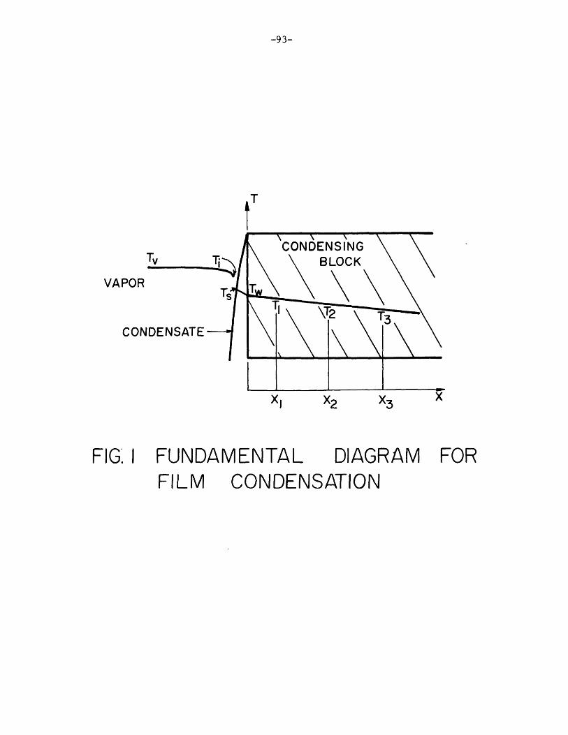
-93-

POR

CONDENSATE-

FIG. I

CONDENSINGCONDENSING

BLOCK

TT

________I________ __________

X2

FUNDAMENTAL

X3

DIAGRAM FORCONDENSATION

VA

FILM

-94-

FROM ARGONSUPPLY CONDENSiNG

SURFACE

VACUUMPUMP

-SECONDCONDENSER

W IIO 2 4

INCHES

FIG 2 SCHEMATICCONVECTION

OF NATURALLOOP

COOLINGTUBE,

1.0

NICKEL BRAZE

FIG. 3 SECTIONAL VIEW OF TESTCONDENSER

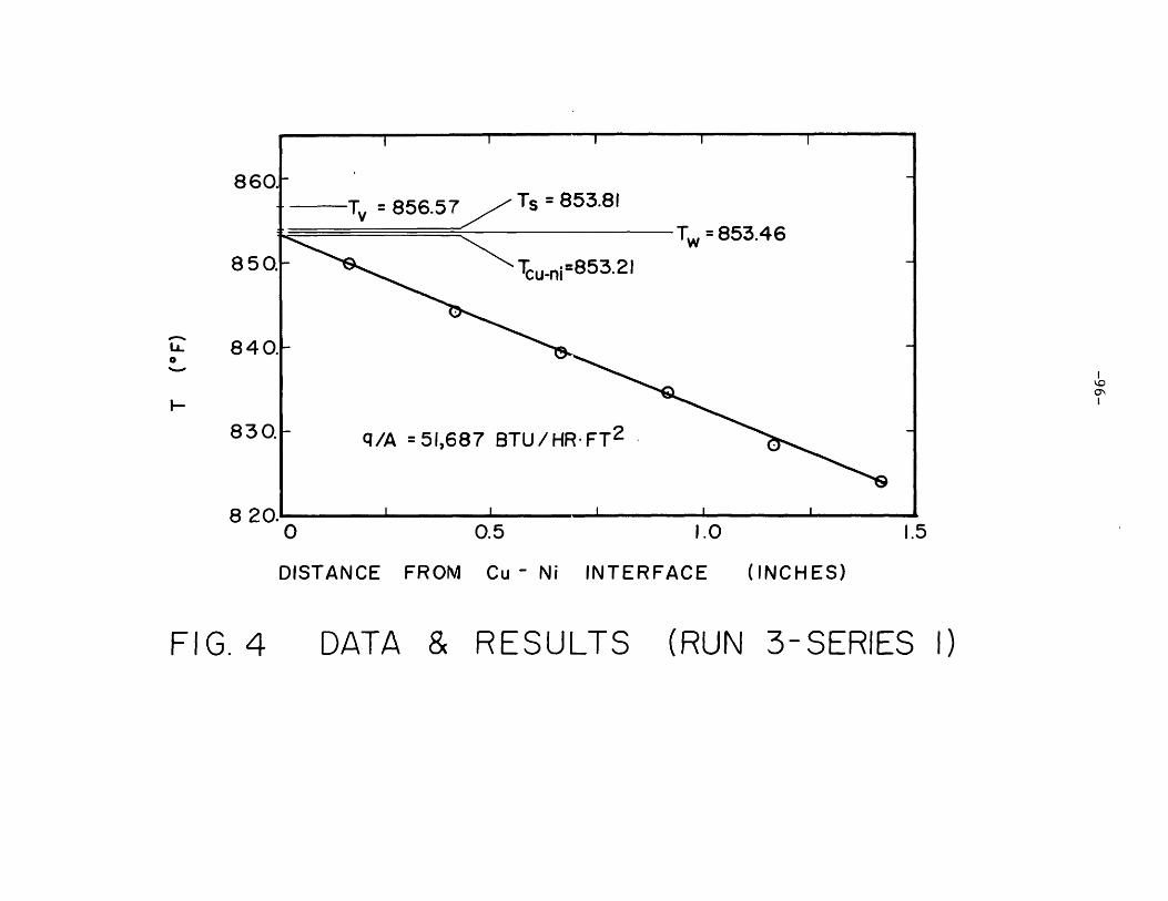
0 0.5 1.0

DISTANCE FROM Cu - Ni INTERFACE (INCHES)

(RUN 3- SERIES

86

85

84

83,

8211.5

FIG. 4 DATA & RESULTS

S0.5 1.0

FIG. 5

DISTANCE

DATA

FROM Cu - Ni INTERFACE

RESULTS

(INCHES)

(RUN 18- SERIES 3)

15

2.0

zJ 1.0 4 AA jA AA M fi- ! A A AAA AA

0 1.0

0+ A~j

oe

0) * PRESENT INVESTIGATION, Kx SUBBOTIN et. al., K [11 t

Z SUBBOTIN et. al., Na 01 O+

o .- + MORIN, MEYRIAL, ROHS ENOW, K [121 0

I KROGER, ROHSENOW, K [13]A SUBBOTIN, et. al., Na 14] 6< SUBBOTIN, et. al., Hg 0J +o b-o SUKHATME, ROHSENOW, Hg 06]

C) > MISRA, BONILLA, Hg [7]Z 4 MISRA, BONILLA, No 07]o o BARRY, Na 081

0.01 o ALADYEV, et. al. K [9]

.0001 .001 .01 0.1 1.0

Pv (ATM)

FIG. 6 SURVEY OF CONDENSATION COEFFICIENTDATA

-99-

0 2 4 6 8 10

(Tv - Ts)CONDENSATIONVS. (Tv - Ts)

COEFFICIENT

b

wF-

-JD0-j

0

0.1L-1

FIG.7

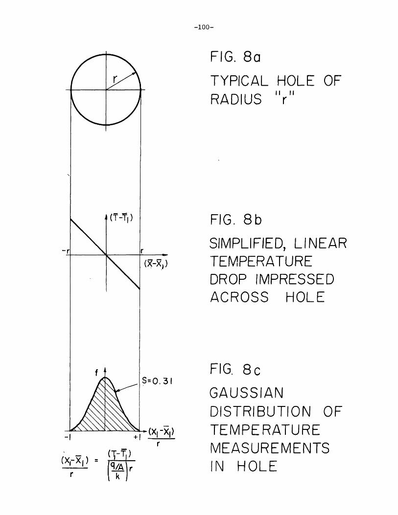
-100-

FIG. 8a

TYPICAL HOLE OFRADIUS r

FIG. 8b

SIMPLIFIED, LINEARTEMPERATUREDROP IMPRESSEDACROSS HOLE

I -xgr

(X-R 1 )

kIr

FIG. 8 c

GAUSSIANDISTRIBUTION OFTEMPERATUREMEASUREMENTSIN HOLE

-101-

(TW - W

f

FI G. 9

TI)

(T q /A

(T2 (- -2)

S(T3-Tf3 )

x x 2 xR3 X

SCHEMATIC REPRESENTATIONOF DISTRIBUTIONS INHOLES AND AT WALL

I I

B-

6-

4

2KROGERST. DEV.

0-5 -2

=53-5.8

Tw -Two/A

Ts - Tslq /AJ

PRESENT SST DEV.

MEYRIALST. DEV =

I I

YSTEM4.8x1O6

[123I.6xlO -

2 5

x 10 /FBTUI/HR-FT2

FIG. 10 PROBABILITY DENSITY FUNCTIONWALL

V~-

10

x

I-

zwZ

AT

........................... I .... I

21 I I I I

(Tv -Ts)(q /A) ,C-4

(* F)

(BTU/HR-FT 2 )10-5

FOR 0-= 1.0

(Ts -Tw)V(q /A)

(*F) 0.75(BTU/HR-FT 2 )

LENGTH=

.001

Pv

1.0"

I I 111111 I I I 11111 I I 11111

.01

(ATM)

FIG. I I EFFECT OF Pv ON (Tv-Ts) & (Ts -Tw)POTASSIUM

FOR

I I I II

II I I . . I II

I

l

-104-

FIG. 12

f Ts(

Ts >Tv

'! ' '1 ' '',% "n TTv (4/A)

(q /A)

OF CONDENSATE

Ts(q /A)

v -Ts)(q/A)

DISTRIBUTIONSURFACE TEMPERATURE

0-6

TV - Tsq/A

ic-4

* F T2)BTU/HiR-FT2

FIG.13 vs. (Tv-Ts)/(q/A)

-105-

10

LL

ILl

106

E [(TV -Ts) / (q/A) I

- I I I I 11111 I I I 111111 I I I 111111 I I 111111 I I I I I IL~

e PRESENT SYSTEMCOPPER (k=210)

- A SUBBOTINCOPPER (k=210)

- 4 KROGER [13- NICKEL (k=28)

- +MEYRIAL 12]S. STEEL (k=12)

.0001 .001

E[a'] FORA PRESENT4L. SYSTEM

E[Oc]KRO

I I liii I i I I till I I I I I till

FORGER

E[O') FORMEYRIAL

I I I lE

.01

Pv (ATM)

& DATA

1.0

05

w0.1

0.01

E[0')F IG. 14

I I 1 1

I I I I I I I I II I I I 1 1 1 1 1

I I I I I I I I I

v S. Pv

I0.

1.0-

0"0

E ['O.I _ MYRIAL [2

)STEEL (k =12)0.5

0.011 Pv =0.3

.0001 .001 .01 0.1 1.0 10.

Pv (ATM)

FIG. 15 PREDICTED DISTRIBUTION OF DATA

I I I I I liii I I I I I liii I I I I III'

I I 11111111

-- - MERCURY

POTASSIUM

SODIUM

I I I I li II I I I II i

.001III I I I I 11111 I i I Iii lu l

.01

PRESENTSYSTEMk = 210

KROGER[13k'=28

MEYRIAL [12k= 12

I0.

(ATM)

FIG. 16 EFFECT OF FLUID ON

1.0

0.I

0.01.0001

Pv

E ']

. . . . . . . . .I I I I I II I I I I I 1 1

I I I i I i I I I I I I I I I I I I I I I I I

- - - -0

1.0

E[ICY] 0.1 r'-

FLUID: WATER

MEYRIAL KROGER [131k=28

k= 120.010.001 0.01 0.1 1.0 10

Pv (ATM)

FIG.17 E [cr VS. Pv FOR WATER

-110-

10

0.91

TV~8 5 0 OFPy : O.Ol7 ATM

qTEST COND. r 600 BTU/HR

I I I I I I ~ ___ I___

500 1000

CONDENSER (BTU/HR)

FIG. 18 EFFECT OF SECONDCONDENSER

/1/0.02 ATM

0.8 ~

0.7 _

0.0

SECOND

AT

I I I I I I I I I L-

-111-

FIG. Al. NATURAL CONVECTION LOOP FIG. A2. LOOP DURING CONSTRUCTION

FIG. A4.ELEMENTS FOR TEST SECTION

FIG. A3. OLD AND NEW APPARATUS

-112-

FIG. A5. TEST SECTION AFTER BRAZING

FIG. A6. ASSEMBLING OF TOP

FIG. A8. PROTECTIVE DRUM IN PLACEFIG. A7. LOOP WITH AUXILIARIES

-113-

750[-

T.C. FROMLEFT SIDE

--w Cu

POSITION

FIG. C-I

BLOCK 2" WIDE

1.0OF T.C. JUNCTION

IMMERSION

20(INCHES)

TEST WITHHOMOGENEOUS T.C.

751

749

-114-

T.C.- LEFT

FROMSIDE

Cu

POSITION

TC. FROMRIGHT SIDE-

BLOCK

IOF TC.

2" WIDE

.0JUNCTION

2.0(INCHES)

FIG. C-2 IMMERSION TEST WITHINHOMOGENEOUS

'F

T C.

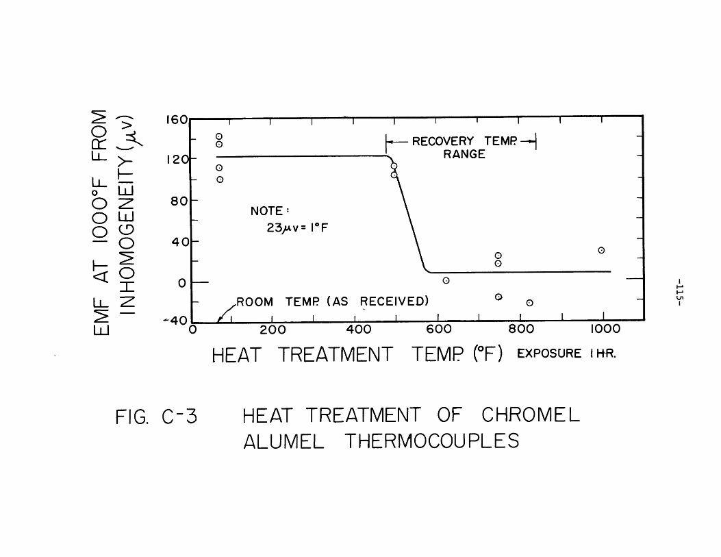
160

|2 0- 0

NOTE:23*v= l*F

0 >H-

o LJ

- Oz

-I-

LLZ

LLJ

TEMP (AS

200

RECOVERY TEMP -HI I I

RECOVERY TEMPRANGE

0O

RECEIVED)

600

TEMP (*F)800

EXPOSURE

1000

IHR.

400

HEAT TREATMENT

FIG. C-3 HEAT TREATMENT OF CHROMELTHERMOCOUPLES

ROOM

Z. ROOM I

80

401

ALUMEL

-116-

FURNACE

FURNACEAT 1000*F

POINT I 1U1POINT

CHROMEL ALUMEL

ICEBATHS

Cu u

POTENTIOMETER

FIG. C-4 SET-UP USED IN TESTSOF HOMOGENEITY

I -I1 1 I 1

I I

SERIES I

I I I I0.01

PV (ATM)

FIG. E-l EFFECT OF Tv DATA -SERIES I

Q I I

0

2.

1.0

0.1 I I ~0.1I ' I

I I I I I I I I I I I

-I

SERIES

| I I I I I I |0.01

Pv (ATM)

FIG. E-2 EFFECT OF Tv DATA -SERIES 2

1.0

0(Y

0.10.II I I l l I I I I I I l l

I I 1 I i I I i I I I I

Er

0.1

Pv (A TM)

FIG. E -3 EFFECT OF Tv DATA - SERIES

-120-

I I I 1

Pv -0.06 ATMTv ~980 0 FqT EST COND.2 850 BTU/HR

I I600

I I1200

qSECOND CONDENSER (BTU/HR)

FIG. .F -I E FFECT OF SECONDCONDENSER AT

I I1.0

0.9

0.8

0

I I1800

I I I I I I I I

I I

0.06 ATM