FII and Its Impact on Stock Market: A Study on Lead-Lag ...

Asian Journal of Finance & Accounting ISSN 1946-052X

2012, Vol. 4, No. 2

www.macrothink.org/ajfa 18

FII and Its Impact on Stock Market: A Study on

Lead-Lag and Volatility Spillover

Dr Namita Rajput (Corresponding Author)

Associate Prof in Commerce

Sri Aurobindo College (m), University Of Delhi

E-mail: [email protected]

Ms Parul Chopra

Research Scholar

Department of management, CMJ, Shilong


Mr Ajay Rajput

Director Marketing, Patil Rail Infrastructure Pvt Ltd


Received: May 30, 2012 Accepted: June 26, 2012 Published: December 1, 2012

doi:10.5296/ajfa.v4i2.1874 URL: http://dx.doi.org/10.5296/ajfa.v4i2.1874

Abstract

In this paper we examine the information spillover and volatility spill-over relationship for Indian stock market. We cover data during 1992-2011. We examine if there has been an increase in volatility persistence in the Indian stock market on after the process of financial liberalization initiated in India. Further, we examine the shifts in stock price volatility and the nature of events that apparently cause the shifts in volatility. We examine if there has been an increase in volatility persistence in the Indian stock market on after the process of financial liberalization initiated in India. This paper explores to develop alternative models from cointegration, VECM, Variance De-composition Analysis, Granger causality, Block Exogeneity wald test, Impulse Response Analysis and alternative forms of the Autoregressive Conditional Heteroscedasticity (ARCH) or its generalisation, the Generalised ARCH (GARCH) family, to estimate volatility in the Indian equity market return. Bidirectional informational spillover is confirmed. The bidirectional volatility spill-over, persistence and


2012, Vol. 4, No. 2


clustering is also confirmed in the sample series. Our findings have implications for policy makers, hedgers and investors. The research contributes to present investment literature for emerging markets such as India.

Keywords: Price discovery, Granger Causality, VECM, EGARCH, Volatility spill over

JEL: G13; G14; G 15; G18; C32; F30


2012, Vol. 4, No. 2


1. Introduction

There are important implications in economics and finance, as regards estimation of volatility in the equity market. There are adverse effects in the economy because of high volatility in the stock prices and can also change the investment decisions by investors due to high volatility, which may lead to a fall in the long-term capital flows from foreign as well as domestic investors. In the last decade financial crisis have exposed that financial asset price volatility has the potential to undermine financial stability. There is empirical evidence to this context that financial stability is in danger more by abrupt shifts in volatility rather than by a sustained increase in the level of volatility. Hence there is an intense need to have the understanding of volatility for risk management in an economy. Indian stock market was opened to Foreign Institutional Investors on 14th September 1992.

The movements in the stock prices are influenced by the flow of market information are well known to everyone and movement in other stock market can be one source. In contemporary world of today because of trading mechanism and investment patterns there can be information spillover of one market to another. Hence return patterns of two different markets might affect each other. Economies are becoming increasingly interrelated and integrating themselves to the world economy because of higher degree of openness in the economies (vide John et. al. (1995).All the decisions of portfolio investment are taken embedding the information relating to these price movements and volatility as regards assets traded. This can lead to reducing or gaining out of diversification across border investment in portfolios. The market traders have to formulate hedging, regulatory and portfolio strategies, for this they have to completely understand the behaviour of the market in the global context. This scenario has led to increased capital flows from FIIs to emerging economies like India with expanding stock market. There are many factors which have led to the growth of financial integration of Indian capital market into world economy like communication technology, computerization of trading system, increased pace of multinational corporations etc. There is a tremendous change in the nature, extent and magnitude of the investment done by theses FIIs. There are diverse view of FIIs investment in emerging economies in general and India in particular; one view is that FIIs are believed to improve market efficiency and helps in lowering the cost of capital the other view holds FIIs responsible for increasing the volatility in stock markets.

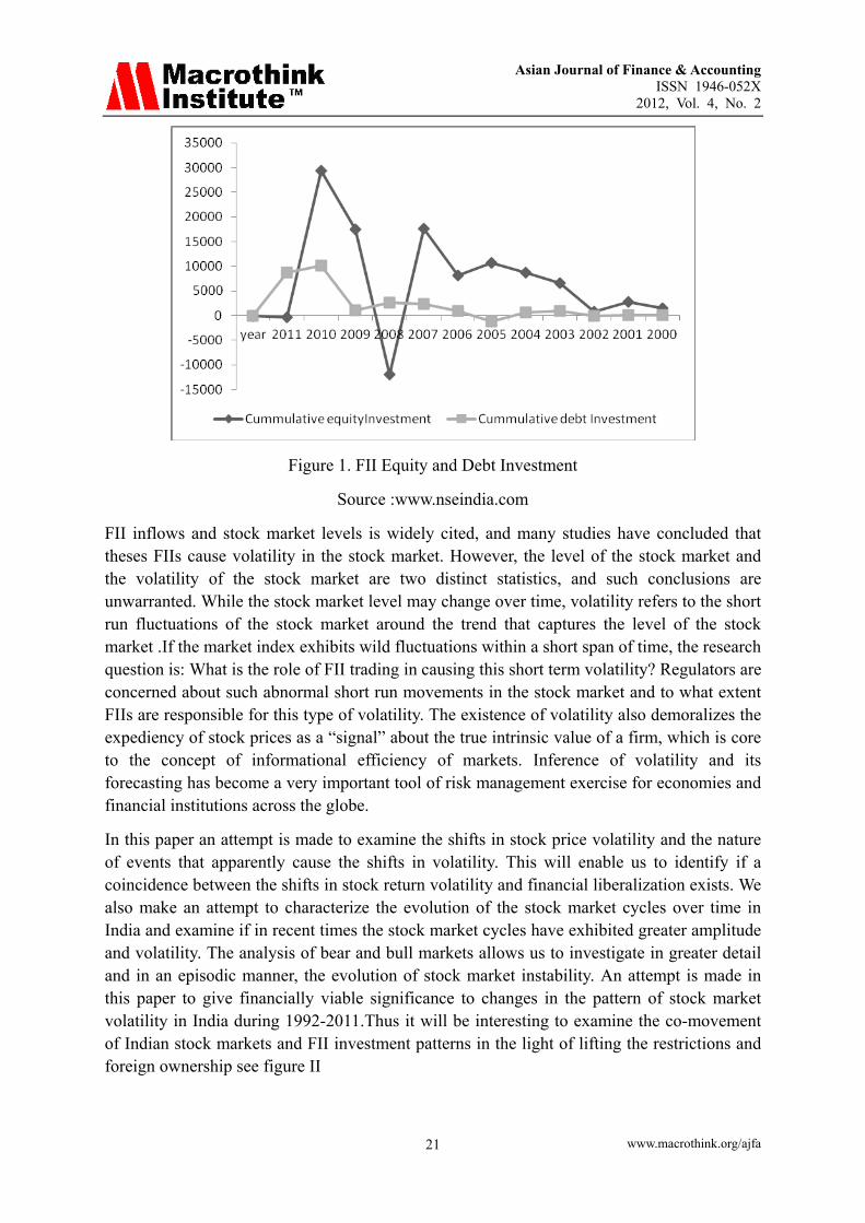
India is considered as a good investment centre after the restrictions are lifted in a liberalised regime. There has been increase in the capital flows into the country which is strong evidence to this context see, figure 1 below.


2012, Vol. 4, No. 2


Figure 1. FII Equity and Debt Investment

Source :www.nseindia.com

FII inflows and stock market levels is widely cited, and many studies have concluded that theses FIIs cause volatility in the stock market. However, the level of the stock market and the volatility of the stock market are two distinct statistics, and such conclusions are unwarranted. While the stock market level may change over time, volatility refers to the short run fluctuations of the stock market around the trend that captures the level of the stock market .If the market index exhibits wild fluctuations within a short span of time, the research question is: What is the role of FII trading in causing this short term volatility? Regulators are concerned about such abnormal short run movements in the stock market and to what extent FIIs are responsible for this type of volatility. The existence of volatility also demoralizes the expediency of stock prices as a “signal” about the true intrinsic value of a firm, which is core to the concept of informational efficiency of markets. Inference of volatility and its forecasting has become a very important tool of risk management exercise for economies and financial institutions across the globe.

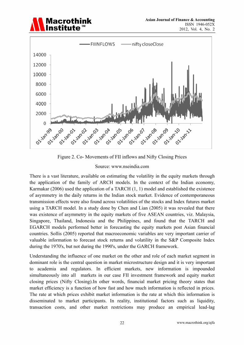
In this paper an attempt is made to examine the shifts in stock price volatility and the nature of events that apparently cause the shifts in volatility. This will enable us to identify if a coincidence between the shifts in stock return volatility and financial liberalization exists. We also make an attempt to characterize the evolution of the stock market cycles over time in India and examine if in recent times the stock market cycles have exhibited greater amplitude and volatility. The analysis of bear and bull markets allows us to investigate in greater detail and in an episodic manner, the evolution of stock market instability. An attempt is made in this paper to give financially viable significance to changes in the pattern of stock market volatility in India during 1992-2011.Thus it will be interesting to examine the co-movement of Indian stock markets and FII investment patterns in the light of lifting the restrictions and foreign ownership see figure II


2012, Vol. 4, No. 2


Figure 2. Co- Movements of FII inflows and Nifty Closing Prices

Source: www.nseindia.com

There is a vast literature, available on estimating the volatility in the equity markets through the application of the family of ARCH models. In the context of the Indian economy, Karmakar (2006) used the application of a TARCH (1, 1) model and established the existence of asymmetry in the daily returns in the Indian stock market. Evidence of contemporaneous transmission effects were also found across volatilities of the stocks and Index futures market using a TARCH model. In a study done by Chen and Lian (2005) it was revealed that there was existence of asymmetry in the equity markets of five ASEAN countries, viz. Malaysia, Singapore, Thailand, Indonesia and the Philippines, and found that the TARCH and EGARCH models performed better in forecasting the equity markets post Asian financial countries. Sollis (2005) reported that macroeconomic variables are very important carrier of valuable information to forecast stock returns and volatility in the S&P Composite Index during the 1970's, but not during the 1990's, under the GARCH framework.

Understanding the influence of one market on the other and role of each market segment in dominant role is the central question in market microstructure design and it is very important to academia and regulators. In efficient markets, new information is impounded simultaneously into all markets in our case FII investment framework and equity market closing prices (Nifty Closing).In other words, financial market pricing theory states that market efficiency is a function of how fast and how much information is reflected in prices. The rate at which prices exhibit market information is the rate at which this information is disseminated to market participants. In reality, institutional factors such as liquidity, transaction costs, and other market restrictions may produce an empirical lead-lag


2012, Vol. 4, No. 2


relationship between price changes in investment scenario or investment behaviour. Besides being of academic interest, understanding information flow across markets is also important for hedge funds, portfolio managers and hedgers for hedging and devising cross-market investment strategies.

Volatility is yet another area of interest both for regulators and for market participants who prefer less volatility to more volatility. A meaningful interpretation of volatility will give us important information and will act as a measure to know as to how far the current prices of an asset deviate from its average past prices. At a fundamental level, volatility specifies the strength or confidence behind a price move. Instinctively, we can argue that the measurement issues of volatility can also be useful to comprehend the market assimilation, co-movement and spill over effect. The existence of volatility spillover between the two markets specifies that the volatility of returns in one market has an important effect on the volatility of returns in the other market. Considerable amount of research work has been conducted in the field of volatility of stock market and FII investment regime and its spillover, but the results of which are mixed. Issues like lead-lag and volatility spillover have been extensively researched for mature markets .Emerging markets in general and India in particular, the work is very limited. In this backdrop, an attempt has been made to revisit the debate on lead-lag, causality and volatility spillover in Indian stock market. Specifically the present study covers empirical analysis both for fairly long study period compared to prior research of the subject and also analysis how the lead-lag, causality and volatility spillover relationships are in Indian context. The study addresses the following question

1. To examine if FII investment are useful in impacting stock market and vice-versa, i.e. a lead lag relationship?

2. Is there a volatility spill over from FII investment patterns to Nifty closing prices and vice-versa?

The remainder of the paper proceeds as follows. Section one describes the theoretical aspect of Indian stock market its importance, relevance, rationale followed by a Section (II) that deals with reviews of the relevant research studies connected with the objectives. Section three entails Data and Methodology describing the nature and sources from which relevant data has been collected and the various statistical tools and techniques employed in the study .Section IV exhibits analysis and interpretation of the data through a variety of tables into which relevant details have been compressed and summarized under appropriate heads and presented in the tables. Section IV briefs the summary and conclusion of the main findings along with the policy implications that emerged from the findings of the study, along with limitations of the study and directions for future research. Section V will list the references cited while undertaking the research.

2. Review of Literature

There are numerous studies that have been explored so far in the ascertainment of whether the FII investment behaviour is reflected in the stock market (closing prices), at various interval of time. Many studies done across the globe are done mainly in context of


2012, Vol. 4, No. 2


transmission of volatility across economies and the contagion effects of a financial crisis which include the work done by Forbes and Rigobon (2002), Bekaert, Harvey and Lumsdaine (2002a,b), Edwards (2000) and others. Rogobon (2003) focus his study on alternative measures of volatility in the equity and bond markets in the period adjacent the financial crises. Bekaert and Harvey (2000) analyse equity returns in a group of emerging economies before and after financial reforms in a group of emerging markets and find mixed results. During 1985-95 in a study done by Aggarwal, Inclan and Leal (1999) analyze volatility in emerging stock markets. ICSS algorithm was used to identify the points of abrupt changes in the variance of returns they examine the nature of events that cause large shifts in stock return volatility in these economies. Local events jumps were held responsible for stock market volatility of the emerging markets by a study done by Aggarwal et al. They find no systematic effect of liberalisation after studying the behaviour of stock prices after the economy was opened to foreigners or large foreign inflows Kim and Singal (1997) & De Santis and Imorohoroglu (1994). The results of this study corroborate Bekaert’s findings that volatility in emerging markets is unrelated to his measure of market integration. Richards (1996) use two sets of data and three types of methodologies to estimate volatility of emerging markets and find no increase in volatility following the process of liberalisation. Levine and Zervos (1995) find results contrary to Richards (1996) that there may increase volatility after liberalisation.

No systematic evidence that foreign trading tends to increase market volatility more than trading by domestic groups was revealed by Hamao and Mei (2001) who examined the impact of foreign and domestic trading on market volatility for Japan. The period of time study mainly relates to the time period during which the foreign portfolio investment in Japan was rather small. The study done by Folkerts – Landau and Ito (1995) on volatility of emerging markets in periods that differ in their intensity of portfolio flows generated mixed results with Mexican stock prices being least volatile when flows are most volatile and vice versa for Hong Kong. Excess volatility was reported by Nilsson (2002) following the process of liberalisation using the Markov regime-switching model. He finds evidence of higher expected return, higher volatility and stronger links with international stock markets characteristic of the deregulated period in all Nordic stock markets. Studies analyzing the behaviour of stock prices over financial cycles have been undertaken in the recent years. It was confirmed in the study that owing to liberalisation the stock markets tend to become more stable. Time varying patterns of financial cycles before and after financial liberalization was examined by Kaminsky and Schumkler (2001, 2002) in 28 countries. The results indicate that more liberalisation cause financial extremes in the short-run and also brings a change in the institutional set up of which will have a supporting and better functioning of financial markets. A temporary rise in volatility was observed in all countries immediately after the liberalisation. In a study done by Edwards et al (2003) ,the stock price behaviour in six emerging economies is analyzed .The results they find exhibit that emerging economies like Korea are in the process of recuperating their stability where as more stable relatively.

2.1 Stock Market Volatility

A study (MT Raju et al (2004) find that the volatility is less in mature markets and provide


2012, Vol. 4, No. 2


very high returns. India and China exhibit high returns where as all other emerging economies exhibit low returns. A study is done on spot price indices of BSE Sensex and S&P CNX Nifty to explain the extent and patterns of stock return volatility. The results exhibits rise in volatility in the period 1990-2000, with a sharp fall in 1992 till 1995, after which there was a sharp rise, however the volatility in the portfolio into India was very small in comparison to other emerging markets, (Gordan J and P Gupta (2003), Harivinder Kaur’s (2004).Stock market volatility plays an imperative role in the financial development as well as growth. Daily volatility is calculated as a standard deviation of the natural log of daily returns on the indices for the respective months. Volatility in stock prices in India, by and large has shown a flagging drift except in few certain months. The market may have turned riskier, messy politics could resurface, and oil prices are at a new high (but at present low); but nothing seems to worry local investors, who feel the index can go up further. Anand Bansal and J.S. Pasricha (2009) studied the impact of market opening to FIIs on Indian stock market behaviour. They empirically analyze the change of market return and volatility after the entry of FIIs to Indian capital market and found that there is no significant change in the Indian stock market average returns; volatility is significantly reduced after India unlocked its stock market to foreign investors.

In the next section we are discussing the data sources and methodology of the study Understanding volatility is therefore central to risk management in an economy. Asymmetry in stock market volatility has its own significance, which implies volatility rises after negative shock than positive shock of similar magnitude. If the stock market is efficient, then the volatility of stock returns should be related to the volatility of the variables that affect asset prices. Stock market volatility tends to be persistent; that is, periods of high volatility as well as low volatility tend to last for months. In particular, periods of high volatility tend to occur when stock prices are falling and during recessions. The relationship of Stock market volatility with that of economic variables like inflation, Industrial production and debt levels in the Indian corporate sector also is positively related to volatility in economic variables, such as inflation, industrial production, and debt levels in the corporate sector (Schwert 1989).

After review the literature, it is quite evident that this issue of volatility of stock returns owing to liberalisation in emerging economies has been studied and examined extensively in the recent years. India is not included in the sample of countries for which liberalization and volatility is analyzed as it was mainly limited to Latin America and East Asia. As mentioned above, empirical literature on lead-lag and volatility spillover mainly deals with developed markets like US and UK. In India significant and relevant literature in this context is thin This paper examines the case for India i.e., the FII investment patterns effectively serves the price discovery function and impacts the Nifty closing prices and vice-versa, and that the introduction of FII equity investment has resulted in volatility in the Nifty closing prices and vice-versa .This study is a modest attempt to fill this gap through our analysis.

3. Data and Methodology

Period of Study :The study spans the period January 1992 to March 2011.This period is very


2012, Vol. 4, No. 2


important as major changes took place in these years and also , major changes were brought about in the structure as well as functioning of the Indian stock markets during this period. Major regulatory changes were made in the light of the scam of 1992 and the information, communication, and entertainment (ICE) meltdown of 2001 like circuit filters were introduced by the NSE, paperless trading was introduced and made compulsory, rolling settlements were introduced in a partial manner, index based futures were introduced ,carry forward of trades was abolished. Hence this period for study is quiet significant owing to these changes ,to have a deep understanding of the volatility patterns .The daily stock price data on Nifty have been taken from PROWESS, the online database maintained by the Centre for Monitoring of Indian Economy (CMIE).CMIE maintains this database for calculating its various indices. The database contains all the actively traded stocks at any given time on the NSE. Daily opening, high, low, and closing prices have been taken for NSE indices for the period of study. These prices have been adjusted for bonus and right issues. Daily stock prices have been converted to daily returns. The present study uses the logarithmic difference of prices of two successive periods for the calculation of rate of return. The logarithmic difference is symmetric between up and down movements and is expressed in percentage terms for ease of comparability with the straightforward idea of a percentage change. If I t be the closing level of nifty on date t and I t-1 be the same for its previous business day, i.e., omitting intervening weekend or stock exchange holidays, then the one day return on the market portfolio is calculated as:

Rt = ln (I t /I t-1) x100

Where, ln (z) is the natural logarithm of ‘z.’

3.1 Econometric Methodology

Given the nature of the problem and the quantum of data, we first study the data properties from an econometric perspective and find that co-integration and error correction models are required to establish the equilibrium relationship between the markets. Further, to quantify and study volatility spill over, we use bivariate EGARCH framework which is covered in the next section. To test the causality block Exogeneity Test is performed the results of which are entailed in Result Section. The regression analysis would yield efficient and time invariant estimates provided that the variables are stationary over time. However, many financial and macroeconomic time series behave like random walk. We first test whether or not the spot and futures price series are co-integrated. The concept of co-integration becomes relevant when the time series being analysed are non stationary. The time series stationarity of sample price series has been tested using Augmented Dickey Fuller (ADF) 1981. The ADF test uses the existence of a unit root as the null hypothesis. To double check the robustness of the results, Phillips and Perron (1988) test of stationarity has also been performed for the series.

4. Analysis and Interpretation of Results

4.1 Lag Relationship of FIIs and Nifty (Information Spillover and Price Discovery)

4.1.1 Tests of Stationarity

The results of stationarity tests are given in Table 1. It confirms non stationarity of Nifty price data & FII equity investment series; hence we repeat stationarity tests on return series


2012, Vol. 4, No. 2


(estimated as first difference of log prices) which are also provided in Table 1. The table describes the sample price series that have been tested using Augmented Dickey Fuller (ADF) 1981. The ADF test uses the existence of a unit root as the null hypothesis. To double check the robustness of the results, Phillips and Perron (1988) test of stationarity has also been performed for the Nifty closing Prices and FII Equity Investment and then both the test are performed on return series also as shown in Panel-A (price series) and Panel B (Return series) are integrated to I (1). The sample return series exhibit stationarity thus conforming that both variables in the sample series are integrated to the first order see Table 1

4.1.2 Tests of Cointegration

If two or more series are themselves non-stationary, but a linear combination of them is stationary, then the series is said to be co-integrated. Given that sample series are integrated of the same order, co-integration techniques are used to determine the existence of a stable long-run relationship between the series. Arrival of new information results in lead-lag, causal relationship for short intervals of time between them due to communication cost. The price linkage between futures market and spot market is examined using cointegration (Johansen, 1991) analysis that has several advantages. First, cointegration analysis reveals the extent to which two markets have moved together towards long run equilibrium. Secondly, it allows for divergence of respective markets from long-run equilibrium in the short run. The co -integrating vector identify the existence of long run equilibrium while error correction dynamics describes the price discovery process that helps the markets to achieve equilibrium (Schreiber and Schwartz, 1986).

Co-integrating methodology fundamentally proceeds with non-stationary nature of level series and minimizes the discrepancy that arises from the deviation of long-run equilibrium. The observed deviations from long-run equilibrium are not only guided by the stochastic process and random shocks in the system but also by other forces like arbitrage process. As a result, the process of arbitrage possesses dominant power in the commodity future market to minimize the very likelihood of the short run disequilibrium. Moreover, it is theoretically claimed that if futures and spot price are coinetgrated, then it implies presence of causality at least in one direction. On the other hand, if some level series are integrated of the same order, it does not mean that both level series are coinetgrated. Cointegration implies linear combinations of both level series cancelling the stochastic trend, thereby producing a stationary series.

Johansen’s cointegration test is more sensitive to the lag length employed. Besides, inappropriate lag length may give rise to problems of either over parameterization or underparametrisation. The objective of the estimation is to ensure that there is no serial correlation in the residuals. Here, Akaike information criterion (AIC) is used to select the optimal lag length and all related calculations have been done embedding that lag length. The cointegration results are reported in Table 2.

Maximal Eigen value and trace test statistics are used to interpret whether null hypothesis of r =0 is rejected at 5% level and not rejected when r =1. Rejection of null hypothesis implies that there exists at least one co-integrating vector which confirms a long run equilibrium


2012, Vol. 4, No. 2


relationship between the two variables, FII equity investment and nifty closing prices in our case. The null hypothesis is rejected Which reveals that one cointegration relationship exists between , FII equity investment and nifty closing prices ,thus they share a share common long-run information.

Despite determining a co integrating vector for each commodity /index, it is customary to produce the diagnostic checking criterions before estimating the ECM model. Diagnostic tests are performed only for those series for which there is a long run relationship confirmed by Johnson cointegration test. Vector Auto Regression (VAR) estimated with various lags selected by AIC is used to check whether the model satisfies the stability, normality test as well as no serial correlation criterion among the variables in the VAR Adequacy model. Testing the VAR adequacy of the sample series as shown in Table 3, it was revealed that all the sample series are satisfying the stability test. In normality test all the sample commodities are found to be normal. In verifying the VAR Residual Serial Correlation LM Tests it was found that in sample series no serial correlation was present. Therefore, it leads us to take the position that our model fulfils the adequacy criterion for sample series which exhibit a long run relationship between the sample series as exhibited by Johansson Cointegration Test. The error correction model takes into account the lag terms in the technical equation that invites the short run adjustment towards the long run. This is the advantage of the error correction model in evaluating price discovery. The presence of error correction dynamics in a particular system confirms the price discovery process that enables the market to converge towards equilibrium. In addition, the model shows not only the degree of disequilibrium from one period that is corrected in the next, but also the relative magnitude of adjustment that occurs in both markets in achieving equilibrium. Moreover, cointegration analysis delivers the message saying how two markets (such as futures and spot commodity markets) reveal pricing information that are identified through the price difference between the respective markets. The implication of cointegration is that the commodities in two separate markets respond disproportionately to the pricing information in the short run, but they converge to equilibrium in the long run under the condition that both markets are innovative and efficient. In other words, the root cause of disproportionate response to the market information is that a particular market is not dynamic in terms of accessing the new flow of information and adopting better technology. Therefore, there is a consensus that price change in one market generates price change in the other market with a view to bring a long run equilibrium relation is:

ttt SF (1)

Equation (1) can be expressed as in the residual form as: ệ

FtSt ệ t (2)

In the above equations Ft and St are FII and stock prices of a commodity in the respective market at time t. Both α and β are intercept and coefficient terms, where as ệt is estimated white noise disturbance term. The main advantage of cointegration is that each series can be


2012, Vol. 4, No. 2


represented by an error correction model which includes last period’s equilibrium error with adding intercept term as well as lagged values of first difference of each variable. Therefore, casual relationship can be gauged by examining the statistical significance and relative magnitude of the error correction coefficient and coefficient on lagged variable. Hence, the error correction model is:

fttftftfft SYFeF 11^

1 (3)

Sttftftsst FYSeS 11^

1 (4)

In the above two equations, the first part et1^

is the equilibrium error which measures how

the dependent variable in one equation adjusts to the previous period’s deviation that arises from long run equilibrium. The remaining part of the equation is lagged first difference which represents the short run effect of previous period’s change in price on current period’s deviation. The coefficients of the equilibrium error, αf and αs signify the speed of adjustment coefficients in FII Equity Investment and Nifty closing prices that claim significant implication in an error correction model. At least one coefficient must be non zero for the model to be an error correction model (ECM). The coefficient acts as an evidence of direction of casual relation and reveals the speed at which discrepancy from equilibrium is corrected or minimized. If, αf is statistically insignificant, the current period’s change in FII investment pattern does not respond to last period’s deviation from long run equilibrium. If both, αf and βf are statistically insignificant; the closing stock price does not Granger cause FIIs. The justification of estimating ECM is to know which sample markets play a crucial role in lead-lag relationship and information flow.

The VECM results are reported in Table IV. It shows that short run dynamics in the price series and price movements in the two markets. The lag length of the series is selected in Vector Error Correction Model (VECM) on the basis of Akaike’s Information Criteria. The residual diagnostics tests; indicate existence of Heteroscedasticity, in the sample series which exhibit cointegration. Thus, t-statistics are adjusted, as well as the Wald test statistics which are employed to test for Granger causality, by the White (1980) heteroscedasticity correction. After correction, we reestimate VECM and from empirical results and it is noticed that in the VECM model, error correction coefficients are significant in both equations (1) and (2) with correct signs, suggesting a bidirectional error correction in sample series. Error Correction Terms (ECTS) also known as mean- reverting price process, provide some insights into the adjustment process of spot and future prices towards long run equilibrium. For the entire period, coefficients of the ECTs are statistically significant between one to two lags, in both equations of Nifty and FIIs as suggested by Akaike Information Criterion (AIC). This implies that once the price relationship of FIIs and nifty closing prices deviates away from the long-run coinetgrated equilibrium, both markets will make adjustments to re-establish the equilibrium condition. The results reveal that error correction terms of FIIs are greater in magnitude than that of Nifty closing prices, which means FIIs makes greater adjustment in order to re-establish


2012, Vol. 4, No. 2


the equilibrium. In other words, Nifty leads the FIIs.

In addition, the empirical results of VEC Granger Causality/Bloc Exogeneity Wald test between the sample series have been examined to check the direction of causality. The results of VEC Granger causality test are also provided in Table 4. There are bi-directional Granger lead relationships between the two markets which are significant at 5% level. These empirical results are consistent with the co-integrating relationships above.

To reconfirm the empirical results of which market whether spot or futures markets have the ability of price discovery and validate the dominant role of the FIIs in price discovery, Variance Decomposition Analysis is done. The Variance Decomposition Analysis measures the percentage of the forecast error of a variable that is explained by another variable. It indicates the relative impact that one variable has upon another variable within the VECM system. The variance decomposition enables us to assess the economic significance of these impacts as the percentages of the forecast error for a variable sum to one. This structure of result showing the information share shows that most of the price changes of FIIs are because of Nifty closing, and more information flows from Nifty to FIIs. The information share and variance decomposition confirms the dominant role of Nifty in information dissemination, the results of which are also shown in Table 4.

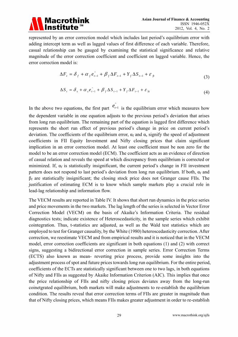
4.1.3 Impulse Response Analysis

The ARMA impulse response view traces the response of the ARMA part of the estimated equation to shocks in the innovation. An impulse response function traces the response to a one-time shock in the innovation. The accumulated response is the accumulated sum of the impulse responses. It can be interpreted as the response to step impulse where the same shock occurs in every period from the first. It gives a graphical view as exhibited by variance Decomposition Analysis.

-10

0

10

20

30

40

50

60

70

1 2 3 4 5 6 7 8 9 10

Response of ENCL to ENCL

-10

0

10

20

30

40

50

60

70

1 2 3 4 5 6 7 8 9 10

Response of ENCL to FIIEQ

0

100

200

300

400

500

600

1 2 3 4 5 6 7 8 9 10

Response of FIIEQ to ENCL

0

100

200

300

400

500

600

1 2 3 4 5 6 7 8 9 10

Response of FIIEQ to FIIEQ

Response to Generalized One S.D. Innovations ± 2 S.E.

It shows a lead role of nifty and FII respond to changes in the movement of Nifty, as is shown in the graph of Response of FIIs to Nifty close. The responses correspond with the result of Variance Decomposition Analysis.


2012, Vol. 4, No. 2


4.2 Volatility Spillover

Volatility is yet another area of interest both for regulators and for market participants who prefer less volatility to more volatility. A meaningful interpretation of volatility will give us important information and will act as a measure to know as to how far the current prices of an asset deviate from its average past prices.

At a fundamental level, volatility specifies the strength or confidence behind a price move. Instinctively, we can argue that the measurement issues of volatility can also be useful to comprehend the market assimilation, co-movement and spill over effect.

The existence of volatility spillover between the two markets specifies that the volatility of returns in one market has an important effect on the volatility of returns in the other market. First the stationarity of data is analysed using Augmented Dickey-Fuller test (ADF) and the results of which are entailed in Table V.

Before estimating the EGARCH model, it is necessary to check the model adequacy by performing the diagnostic tests that involve serial correlation, normally distributed error and goodness of fit measures. All diagnostic tests are primarily carried on the standardized residuals via OLS and it is found that all are significant at 5% level. The diagnostic statistics with respect to EGARCH model are not reported here to conserve space. The results of Volatility spill over relationships between FIIs and Nifty using bivariate E-Garch model are reported in table 6 for entire sample series. The coefficient βsf indicates the volatility spillover from FIIs to Nifty and βfs means reverse direction. The coefficients βss βff show the volatility clustering, while the coefficients Ƴs (stock market) &Ƴf (FIIs) measure the degree of volatility persistence. The residuals of the model are tested for additional ARCH effects using ARCH LM test.

The coefficients of β sf and β fs are very important and reveal volatility spill over from the stock market to fiis or fiis to stock. Results support the bidirectional volatility spillover process with significant coefficients. Volatility persistence is tested for sample series to test the effect of shocks, which is an indicator of market efficiency. It means Persistence of volatility that today’s volatility is due to information that arrived today and will affect tomorrow’s volatility and volatility of days to come. γf and γs measure the persistence of volatility in spot and futures market. The smaller the absolute value of the coefficient, the less persistent volatility is after a shock. Volatility persistence is significant for both stock market (nifty) and fiis for sample series, as p (value) is coming less than 0.05.

Volatility estimation is important for several reasons and for different people in the market pricing of securities is supposed to be dependent on volatility of each asset. Market prices tend to exhibit periods of high and low volatility. This sort of behaviour is called volatility clustering. Volatility clustering is tested for the sample, which means as noted by Mandelbrot (1963), “large changes tend to be followed by large changes, of either sign, and small changes tend to be followed by small changes.” A quantitative manifestation of this fact is that, while returns themselves are uncorrelated, absolute returns |rt| or their squares display a positive, significant and slowly decaying autocorrelation function: corr (|rt|,|rt+τ |) > 0 for τ


2012, Vol. 4, No. 2


ranging from a few minutes to a several weeks. The market-specific volatility clustering

coefficients are all positively significant at 5% level in the fiis and stock

markets. Of course, we can understand the efficiency degree in stock-fiis market from one side according to the magnitude of correlative coefficients. Therefore, the Bivariate EGARCH model indicates that past innovations in fiis significantly influence stock market volatility and vice versa. Finally ARCH Lagrange Multiplier (LM) tests are used to test whether the standardized residuals of bivariate E-Garch model exhibit additional ARCH. The results reveal that EGARCH (1, 1) capture the entire volatility dynamics see Table VII.

5. Summary and Conclusions

Foreign institutional investors have gained a significant role in Indian stock markets. The dawn of 21st century has shown the real dynamism of stock market and the various benchmarking of Nifty index in terms of its highest peaks and sudden falls. The literature relating to information spillover and volatility spillover is not adequately researched in India and is mainly confined to developed economies. Empirical Studies on the subject will reduces informational asymmetries in the market. The present study evaluates informational spillover and volatility spillover effects in Indian stock market to bridge the important gap in the literature. We find that stock market and FIIs prices of all sample commodities and indices are non stationary, and in fact integrated to order one and the Long run equilibrium relationship is confirmed using Johansson cointegration procedure. These cointegration results are supported by VAR adequacy test. Short term dynamics in the series are examined using VECM. The results show that once price relationship of stock and FIIs market deviates away from the long run coinetgrated equilibrium, both markets will make adjustments to re-establish the equilibrium with FIIs is greater in magnitude than that of stock market which implies that FIIs makes greater adjustment in order to re-establish the equilibrium. The results of VEC Granger causality test show bi-directional Granger lead relationships between the sample series. The Variance Decomposition and Impulse responses results reconfirm the dominant role of Nifty in information flow for these series. Next, we examine the volatility spillover effects for sample series to verify whether any risk transfer mechanism can work between stock market and FIIs. E-Garch results confirm bivariate volatility spillover. Thus efficient hedging as well as speculation strategies can be formed for theses commodities. Our results are in conformity to the studies like Levine and Zervos (1995), ,Nilsson (2002), Edwards et al (2003), Gordan J and P Gupta (2003), MT Raju et al (2004) Harivinder Kaur’s (2004) which find that there may increase volatility after liberalisation and in contrary to the studies like De Santis and Imorohoroglu (1994), Richards (1996) .Kim and Singal (1997), Hamao and Mei (2001), Kaminsky and Schumkler (2001, 2002), Anand Bansal and J.S. Pasricha (2009) in which no systematic evidence was found in increasing of volatility in emerging markets i.e. unrelated to the measure of market integration. We conclude that Indian stock market is still not perfectly competitive. Hence there is an urgent need that the policy makers support these trading platforms with infrastructure development, fiscal incentives, encouraging product innovation, widening investor base and investor education so that they are able to realise their true potential.


2012, Vol. 4, No. 2


References

Aggarwal, R., C.Inclan, & R. Leal (1999). Volatility in Emerging Stock Markets. Journal of Financial and Quantitative Analysis, 34(1), 33-35. http://dx.doi.org/10.2307/2676245

Andreou Elena, & Eric Ghysels (2002). Detecting Multiple Breaks in Financial Market volatility Dynamics. Discussion Paper 2002-02, Department of Economics, University of Cyprus.

Anand Bansal, & J. S. Pasricha(2009), Foreign Institutional Investors Impact On Stock Prices in India. Journal of Academics Research in Economics, 1(2), 181-189

Bai, Jushan, & Pierre Perron, (1998). Estimating and Testing Linear Models with Multiple Structural Changes. Econometrica, Econometric Society, 66(1), 47-78. http://dx.doi.org/10.2307/2998540

Bai, Jushan, & Pierre Perron (2003). Critical Values for Multiple Structural change Tests. Econometrics Journal, 6, 72-78. http://dx.doi.org/10.1111/1368-423X.00102

Bekaert, Geert, & Campbell R. Harvey (2000). Foreign Speculators and Emerging Equity Markets. The Journal of Finance, 55 (2), 565-613. http://dx.doi.org/10.1111/0022-1082.00220

Bekaert, G., Harvey, C.R., & R.L. Lumsdaine (2002). The Dynamics of Emerging Market Equity Flows. Journal of International Money and Finance, 21, 295-350. http://dx.doi.org/10.1016/S0261-5606(02)00001-3

Bekaert, G., Harvey, C.R., & R.L. Lumsdaine (2002). Dating the Integration of World Capital Markets. Journal of Financial Economics, 65, 203-249. http://dx.doi.org/10.1016/S0304-405X(02)00139-3

Bekaert, G., Harvey, C.R., & A. Ng (2002). Market Integration and Contagion. Mimeo. Journal of Development Economics, 66, 465-504. http://dx.doi.org/10.1016/S0304-3878(01)00171-7

Biscarri, Javier Gómez, & Fernando Pérez de Gracia (2003). Stock Market Cycles and Stock Market Development in Spain. Facultad de Ciencias Económicas y Empresariales Universidad de Navarra, Working Paper.

Black, Fischer. (1976). Studies of Stock Price Volatility changes. Proceedings of the American Statistical Association Annual Meetings.

Cecchetti, S. P.Lam, & N. Mark (1990). Mean Reversion in Equilibrium Asset Prices. American Economic Review, 80(3), 398 – 418.

Chen, W.Y., & Lian, K.K. (2005). A comparison of forecasting models for ASEAN equity markets. Sunway Academic Journal. 2, 1-12.

De Santis, Giorgio, & S. Imrohoroglu (1997). Stock Returns and Volatility in Emerging Financial Markets. Journal of International Money and Finance, 16(4), 561-579.


2012, Vol. 4, No. 2


http://dx.doi.org/10.1016/S0261-5606(97)00020-X

Edwards, Sebastian, Javier Gómez Biscarri, & Fernando Pérez de Gracia. (2003). Stock market cycles, Financial liberalization and volatility. Journal of International Money and Finance, 22, 925–955. http://dx.doi.org/10.1016/j.jimonfin.2003.09.011

Edwards, Sebastian, Javier Gómez Biscarri, & Fernando Pérez de Gracia. (2003). Stock Market Cycles, Financial Liberalization and Volatility. National Bureau for Economic Research Working Paper No. 9817.33.

Edwards, Sebastian, & Raul Susmel. (2000). Interest Rate Volatility and Contagion in Emerging Markets: Evidence from the 1990s. National Bureau for Economic Research Working Paper No. 7813.

Engle, Robert, & C. Mustafa. (1992). Implied ARCH Models from Options Prices. Journal of Econometrics, 52. 289-311. http://dx.doi.org/10.1016/0304-4076(92)90074-2

Folkerts-Landau, D., & T. Ito. (1995). International Capital markets: Developments, Prospects and Policy Issues. International Monetary Fund, Chapter I and Chapter VII in I. Background papers.

Forbes, Kristin J., & Roberto Rigobon. (2002). No Contagion, Only Interdependence: Measuring Stock Market Co movements. Journal of Finance, 57(5), 2223-2261. http://dx.doi.org/10.1111/0022-1082.00494

Hamilton J.D., & R. Susmel. (1994). Autoregressive Conditional Heteroscedasticity and Changes in Regime. Journal of Econometrics, 64(1-2), 307-333. http://dx.doi.org/10.1016/0304-4076(94)90067-1

Inclan, Carla, & George C. Tiao. (1994). Use of Cumulative Sums of Squares for Retrospective Detection of Changes of Variance. Journal of the American Statistical Association, 89(427), 913-923.

Kaminsky Graciela Laura, & Sergio L. Schmukler. (2002). Short-Run Pain, Long-Run Gain: The Effects of Financial Liberalization. NBER Working Paper 9787 (Cambridge, MA: National Bureau for Economic Research).

Kaminsky, G., Reinhart, C. (2002). Financial Markets in Times of Stress. Journal of Development Economics, 69(2), 451–470. http://dx.doi.org/10.1016/S0304-3878(02)00096-2

Kaminsky, Graciela, & Sergio Schmuckler. (1999). On Booms and Crashes: Stock Market Cycles and Financial Liberalization. Working paper, George Washington University.

Karmakar, M. (2006). Stock Market Volatility in the Long-run, 1961- 2005. Economic and Political Weekly, 41(18), 1796- 1802. http://www.jstor.org/stable/4418179

Kim, E.H., & V. Singal (1994). Opening up of Stock Markets: Lessons from Emerging Economies. Mitsui Life Financial Research Center, Working Paper No 93-18. http://ssrn.com/abstract=5429


2012, Vol. 4, No. 2


Kwan, B.F., & M.G. Reyes. (1997). Price Effects of Stock market Liberalization in Taiwan. The Quarterly Review of Economics and Finance, 37(2), 511-522. http://dx.doi.org/10.1016/S1062-9769(97)90040-5

Lamoureux, Christopher G., & William D. Lastrapes. (1990). Persistence in Variance, Structural Change and the GARCH Model. Journal of Business and Economic Statistics, 8(2), 225-234. http://dx.doi.org/10.2307/1391985

Lastrapes, W.D. (1989). Exchange Rate Volatility and US Monetary Policy: An ARCH Application. Journal of Money, Credit and Banking, 21(1), 66-77. http://dx.doi.org/10.2307/1992578

Lanne, M., & Saikkonen Pentti (2005). Nonlinear GARCH Models for Highly Persistent Volatility. Econometrics Journal, 8, 251–276. http://dx.doi.org/10.1111/j.1368-423X.2005.00163.x

Levine, Ross, & Sara J. Zervos (1998). Capital Control Liberalization and Stock Market Development. World Development, 26(7), 1169–83. http://dx.doi.org/10.1016/S0305-750X(98)00046-1

Maekawa, Koichi, Sangyeol Lee, & Yasuyoshi Tokutso. (2005). A Note on Volatility Persistence and Structural Changes in GARCH Models. Technical report, University of Hiroshima, Faculty of Economics.

Maekawa, Koichi, Sangyeol Lee, & Yasuyoshi Tokutso. (2003). Structural Change and Spurious Volatility Persistence. Discussion Paper, Faculty of Economics, Hiroshima University.

Nilsson, Birger. (2002). Financial Liberalization and the Changing Characteristics of Nordic Stock Returns. Working Papers 2002:4, Lund University, Department of Economics.

Pagian, Adrian, R., & Kirill A. Sossounav. (2003). A Simple Framework for Analyzing Bull and Bear Markets. Journal of Applied Econometrics, 18(1), 23–46. http://dx.doi.org/10.1002/jae.664

Rigobon, R. (2003). On the Measurement of International Propagation of Shocks: Is it Stable? Journal of International Economics, 61, 261-283. http://dx.doi.org/10.1016/S0022-1996(03)00007-2

Shenbagaraman, Premalata. (2003). Do Futures and Options Trading Increase Stock Market Volatility. NSE Research Initiative. http://www.nseindia.com/content/research/Paper60.pdf

Sollis, R. (2005). Predicting returns and volatility with macro-economic variables: evidence from tests of encompassing. John Wiley & Sons Ltd. Journal of Forecasting. 24(3), 221-231. http://dx.doi.org/10.1002/for.956

Shiller, R.J. (1989). Market Volatility. MIT Press, Cambridge, MA.

Tauchen, George E., & Mark Pitts. (1983). The Price Variability – Volume Relationship on Speculative Markets. Econometrica, 51(2), 485- 505. http://dx.doi.org/10.2307/1912002


2012, Vol. 4, No. 2


Wang, Shiyun. (2011). High Frequency Returns - Mean Reversion and Volatility Persistence. Research at the ICMA Centre, Discussion Papers, University of Manchester.

Yardeni, Edward, Joseph Abbott, & Amalia F. Quintana. (2002). Earnings Month. Prudential Financial Research

Table 1. Stationarity Test for Sample series

NAME Panel-A

Panel-B

(ADF) Test Phillips-Perron Test (ADF) Test Phillips-Perron Test

T-Statistics T-Statistics T-Statistics** T- Satistics**

Total FII INVESTMENT -1.09 -0.51 -41.98 ** -41.98 **

NIFTY CLOSING PRICE 1.12 -1.38 -41.35 ** -41.32 **

The table describes the sample price series that have been tested using Augmented Dickey Fuller (ADF) 1981. The

ADF test uses the existence of a unit root as the null hypothesis. To double check the robustness of the results,

Phillips and Perron (1988) test of stationarity has also been performed for the price series and then both the test

are performed on return series also as shown in Panel-A (price series) and Panel B (Return series) are integrated

to I(1). All tests are performed using 5%level of significance (**).

Table 2. Johansen’s Cointegration Test

NAME Hypothesis Lag

Length

Trace Critical

Value**

R=0,

Accept

R=1

Reject

Null Alternate Criterion

(Sc)

Max Eigen

value

Statistic 5 % Sig

Level

FII Equity Investment & Nifty

Closing Price

r =0 r ≥1 4 lags* 0.1249 362.5 15.49 Reject

The table provides the Johansen’s co-integration test, maximal Eigen value and Trace test statistics are used to

interpret whether null hypothesis of r=0 is rejected at 5 % level and not rejected where r=1. Rejection of null

hypothesis implies that there exists at least one co-integrating vector which confirms a long run equilibrium

relationship between the two variables


2012, Vol. 4, No. 2


Table 3. Adequacy Test for VAR Model

Name of Series Var Adequacy Test Critical Values Lags

FII Equity Investment &Nifty

Closing Prices 1

Stability (modulus values of roots of

characteristics polynomials

0.94,.89, 0.24, 0.081

(Stable) 4*

2 Normality Chi-Square values

4.81 (Jarque-Bera) P Val

(0.0900)( Normal) 4*

3 Serial Correlation LM-Test

18.55( p val 0.0806) (no

serial correlation) 4*

The asterisk (*) shows significance at 1, 2, 3 and 4 lags. Diagnostic tests are performed for sample series. Vector Auto

Regression (VAR) estimated with various lags selected by AIC is used to check whether the model satisfies the stability,

normality test as well as no serial correlation criterion among the variables in the VAR Adequacy model. Results

reveal that the sample series are satisfying the stability In normality test the sample series are found to be normal. In

verifying the VAR Residual Serial Correlation LM Tests it was found that in all sample series no serial correlation was

present. Therefore, it leads us to take the position that our model fulfils the adequacy criterion

Table 4. Results of VECM, Variance Decomposition Analysis and Block Exogeneity Tests

Panel (1) Vecm

Indexes Fiis Nifty Close

Error Correction: ∆Ft ∆St

7.12** -1.05**

Cointeq1 (0.48) (0.05)

[ 14.62] [-20.17]

Panel (1 A) : Causality Test

Variables Nifty Close Fii S

Variance Decomposition Analysis 64.01% 35.9%

Block Exogenity Tests Dependent Variable: Dependent Variable:

Var Granger Causality/Block Exogeneity Wald Tests FII Nifty Close

P(0.00) P(0.00)

T-statistics values which are indicated in the parenthesis. A (**) is significant at 5%. This table exhibits short run

dynamics using VECM Model in the price series and price movements in the two markets using Akaike’s

Information Criteria. After correction residuals it was noticed that in the VECM model, error correction

coefficients are significant in both equations, suggesting a bidirectional error correction and Nifty price leads the

FIIs .The results are reconfirmed by Variance Decomposition Analysis confirming the lead role of Nifty. There are

bi-directional Granger lead relationships between Nifty closing and FIIs.


2012, Vol. 4, No. 2


Table 5. Results of Unit root statistics

Name Panel-A Panel-B

(ADF) Test Phillips-Perron

Test

(ADF) Test Phillips-Perron

Test

T-Statistics T-Statistics T-Statistics** T- Satistics**

Total FII Investment -1.09 -0.51 -41.98 ** -41.98 **

Nifty Closing Price 1.12 -1.38 -41.35 ** -41.32 **

Nifty Turnover 0.78 0.65 -32.96 ** -42.7 **

Note: ** statistics significant at 5 % level and are i(1)as regards fii,nifty closing,turnover .

Table 6. Results of Volatility Relationships

Name dependent variable: stdstock

fiis &nifty coefficient std. Err z-stat prob.

a.βss (volatility clustering) Lagstockest -0.01 0.13 -0.10 0**

b.βsf (volitiity spillover) Lagstockest 0.0 0.13 0.03 0**

c.ʏs (volatility persistence) Lagstdstock 0.10 0.02 7.39 0**

dependent variable: stdfiis

a.βff (volitiity clustering) Lagfiiest 0.01 0.13 0.09 0**

b.βfs (volitiity spillover) Lagfiiest -0.00 0.13 -0.05 0**

c.ʏ f (volatility persistence) Lagstdfii 0.10 0.02 7.41 0**

Note: Table describes volatility spillover (βsf and βfs ) volatility persistence (Ƴf and Ƴs) and volatility clustering (βff

and βss) from the stock market(nifty) to fiis or fiis to stock respectively. Volatility spill over is observed .Volatility

persistence is significant for both stock market and fiis for sample series , as p (value) is coming less than 0.05.

The market-specific volatility clustering coefficients βff and βss are all positively significant at 5% level in the

sample series.

Table 7. Arch LM-Test

Commodity coefficient std. error t-statistic prob.

1.comdex

dependent variable: std stock(nifty) std_resid^2(-1) 0.04 0.02 2.11e+00 [0.23]

dependent variable: stdfiis std_resid^2(-1) 0.05 0.02 2.15 [0.3]

FII and Its Impact on Stock Market: A Study on Lead-Lag ...

Documents