Field-Site Prototype for HABIT (FSP-HABIT) Characterizing Martian salts prior to the ExoMars 2020 mission Johannes Milan Güttler Space Engineering, masters level (120 credits) 2016 Luleå University of Technology Department of Computer Science, Electrical and Space Engineering

Welcome message from author
This document is posted to help you gain knowledge. Please leave a comment to let me know what you think about it! Share it to your friends and learn new things together.
Transcript

Field-Site Prototype for HABIT
(FSP-HABIT)
Characterizing Martian salts prior to the ExoMars 2020 mission
Johannes Milan Güttler
Space Engineering, masters level (120 credits)
2016
Luleå University of Technology
Department of Computer Science, Electrical and Space Engineering

Abstract
One of the major remaining question about Mars is its habitability - if the requirements necessary to allowfor life are presently fulfilled. One of the most relevant ingredients for life, as we know it, is water. Indirectevidence of transient liquid water on Mars has been retrieved from both rover [Martın-Torres et al., 2015]and orbiter [Ojha et al., 2015].
[Martın-Torres et al., 2015] inferred the existence of an active water cycle, driven by chlorate and per-chlorate salts, which are commonly found on the Martian surface, and absorb atmospheric water to formstable hydrated compounds and liquid solutions. This happens through a process called deliquescence(absorption of moisture from the atmosphere by the salts and dissolving into a liquid solution). One ofthe goals of HABIT is to confirm the hypothesis about the water cycle on Mars. HABIT will recordthe behavior of a selection of salts on Mars, and will also record Martian environmental conditions (UVdose, air and ground temperatures).
The Field-Site Prototype for HABIT (FSP-HABIT) was the first prototype of HABIT deployed dur-ing field-site campaigns. Three campaigns took place during summer 2016: First, a short preparatorycampaign in Abisko, Sweden, was carried out. The second campaign took place in Iceland, within theEU COST Action TD1308 ORIGINS (Origins and evolution of life on Earth and in the Universe), andthe third campaign was conducted within the NASA Spaceward Bound India Program in Ladakh. Afterproviding the corresponding background on the mission framework and the scientific background, thisdocument covers the mechanical, electrical, and software design of the instrument. Afterwards, the stepstaken to test the instrument and their results are covered, followed by a rating of the instrument and ideasfor future improvements. Instruments like FSP-HABIT will enable the characterization of hygroscopicsalts by their conductivity as liquid brines are good conductors, hydrated salts are poor conductors, anddehydrated salts are insulators. During the field-site campaigns, the measurements of FSP-HABIT wereused to characterize the near surface environment by its temperature, pressure and relative humidity.Now, these measurements are available for comparison with microbiological studies of the water, iceand soils to characterize the habitability of the explored site. The lessons learned while designing andbuilding FSP-HABIT can be used to inform the development of further prototypes for space missionssuch as HABIT.
II

Contents
Abstract II
Contents III
List Of Figures V
List Of Tables VII
Acronyms VIII
Disclosure X
Acknowledgements XI
I INTRODUCTION 1
1 ExoMars 2020, HABIT, And FSP-HABIT 2
2 Scientific Background 42.1 Water On Mars . . . . . . . . . . . . . . . . . . . . . . . . . . . . . . . . . . . . . . . . . . 6
2.1.1 Relative Humidity (RH) . . . . . . . . . . . . . . . . . . . . . . . . . . . . . . . . . 72.2 The Water-Chlorine Correlation . . . . . . . . . . . . . . . . . . . . . . . . . . . . . . . . . 82.3 Brines And Transient Liquid Water . . . . . . . . . . . . . . . . . . . . . . . . . . . . . . . 92.4 Conductivity . . . . . . . . . . . . . . . . . . . . . . . . . . . . . . . . . . . . . . . . . . . 11
3 Instrument Overview 143.1 Mission Statement . . . . . . . . . . . . . . . . . . . . . . . . . . . . . . . . . . . . . . . . 143.2 Instrument Objectives . . . . . . . . . . . . . . . . . . . . . . . . . . . . . . . . . . . . . . 143.3 Instrument Concept . . . . . . . . . . . . . . . . . . . . . . . . . . . . . . . . . . . . . . . 15
II INSTRUMENT DESCRIPTION 17
4 Mechanical Design 184.1 Brines Container Assembly (BCA) Overview . . . . . . . . . . . . . . . . . . . . . . . . . 184.2 Brines Container Assembly (BCA) Detail . . . . . . . . . . . . . . . . . . . . . . . . . . . 19
4.2.1 Brines Container . . . . . . . . . . . . . . . . . . . . . . . . . . . . . . . . . . . . . 194.2.2 Cable Canal And ATS Mount (CCAM) . . . . . . . . . . . . . . . . . . . . . . . . 214.2.3 Filter Fixation And Mount, Filters . . . . . . . . . . . . . . . . . . . . . . . . . . . 224.2.4 Lid . . . . . . . . . . . . . . . . . . . . . . . . . . . . . . . . . . . . . . . . . . . . . 22
4.3 Electrodes . . . . . . . . . . . . . . . . . . . . . . . . . . . . . . . . . . . . . . . . . . . . . 234.4 Electronics Box Assembly (EBox) Overview . . . . . . . . . . . . . . . . . . . . . . . . . . 284.5 Electronics Box Assembly (EBox) Detail . . . . . . . . . . . . . . . . . . . . . . . . . . . . 29
4.5.1 EBox Main . . . . . . . . . . . . . . . . . . . . . . . . . . . . . . . . . . . . . . . . 294.5.2 EBox Lid . . . . . . . . . . . . . . . . . . . . . . . . . . . . . . . . . . . . . . . . . 304.5.3 ARDUINO And Battery Lids; Legs . . . . . . . . . . . . . . . . . . . . . . . . . . . 31
4.6 Material . . . . . . . . . . . . . . . . . . . . . . . . . . . . . . . . . . . . . . . . . . . . . . 32
III
5 Electrical Design 335.1 ARDUINO . . . . . . . . . . . . . . . . . . . . . . . . . . . . . . . . . . . . . . . . . . . . 335.2 Electric Conductivity Sensor . . . . . . . . . . . . . . . . . . . . . . . . . . . . . . . . . . 34
5.2.1 AC Signal Generator . . . . . . . . . . . . . . . . . . . . . . . . . . . . . . . . . . . 345.2.2 Analog Switches . . . . . . . . . . . . . . . . . . . . . . . . . . . . . . . . . . . . . 365.2.3 Voltage Divider . . . . . . . . . . . . . . . . . . . . . . . . . . . . . . . . . . . . . . 375.2.4 Voltage Follower . . . . . . . . . . . . . . . . . . . . . . . . . . . . . . . . . . . . . 395.2.5 Rectifier . . . . . . . . . . . . . . . . . . . . . . . . . . . . . . . . . . . . . . . . . . 395.2.6 Combined Circuit . . . . . . . . . . . . . . . . . . . . . . . . . . . . . . . . . . . . 40
5.3 Environmental Sensors . . . . . . . . . . . . . . . . . . . . . . . . . . . . . . . . . . . . . . 425.3.1 Ground Temperature Sensor (GTS) . . . . . . . . . . . . . . . . . . . . . . . . . . 425.3.2 Relative Humidity Sensor (RHS) . . . . . . . . . . . . . . . . . . . . . . . . . . . . 435.3.3 Pressure Sensor (PS) . . . . . . . . . . . . . . . . . . . . . . . . . . . . . . . . . . . 445.3.4 Air Temperature Sensor (ATS) . . . . . . . . . . . . . . . . . . . . . . . . . . . . . 45
5.4 Power System . . . . . . . . . . . . . . . . . . . . . . . . . . . . . . . . . . . . . . . . . . . 465.5 GSM Cellular Connectivity . . . . . . . . . . . . . . . . . . . . . . . . . . . . . . . . . . . 475.6 SD Card Reader . . . . . . . . . . . . . . . . . . . . . . . . . . . . . . . . . . . . . . . . . 48
6 Software 49
III RESULTS 51
7 Prototype Development 52
8 Testing 558.1 Laboratory Salt Tests . . . . . . . . . . . . . . . . . . . . . . . . . . . . . . . . . . . . . . 55
8.1.1 Preparation . . . . . . . . . . . . . . . . . . . . . . . . . . . . . . . . . . . . . . . . 558.1.2 Corrosion Tests, June 2016 . . . . . . . . . . . . . . . . . . . . . . . . . . . . . . . 55
8.2 Abisko Preparatory Campaign, May 1-4 . . . . . . . . . . . . . . . . . . . . . . . . . . . . 578.3 Iceland Campaign . . . . . . . . . . . . . . . . . . . . . . . . . . . . . . . . . . . . . . . . 588.4 India Campaign . . . . . . . . . . . . . . . . . . . . . . . . . . . . . . . . . . . . . . . . . . 64
8.4.1 Hunder Dunes, 12.08.2016 . . . . . . . . . . . . . . . . . . . . . . . . . . . . . . . . 658.4.2 Kardung La, 13.08.2016 . . . . . . . . . . . . . . . . . . . . . . . . . . . . . . . . . 688.4.3 Sundo Lake, 15.08.2016 . . . . . . . . . . . . . . . . . . . . . . . . . . . . . . . . . 718.4.4 Tso Kar Village, 16.08.2016 . . . . . . . . . . . . . . . . . . . . . . . . . . . . . . . 748.4.5 Taglang La, 17.08.2016 . . . . . . . . . . . . . . . . . . . . . . . . . . . . . . . . . . 77
8.5 Assessment . . . . . . . . . . . . . . . . . . . . . . . . . . . . . . . . . . . . . . . . . . . . 80
9 Prototype Success Rate 83
10 Conclusions And Outlook 87
Bibliography 90
Appendix A India Campaign: ENVPACK data 94A.1 Hunder Dunes, 12.08.2016 . . . . . . . . . . . . . . . . . . . . . . . . . . . . . . . . . . . . 94A.2 Kardung La, 13.08.2016 . . . . . . . . . . . . . . . . . . . . . . . . . . . . . . . . . . . . . 95A.3 Sundo Lake, 15.08.2016 . . . . . . . . . . . . . . . . . . . . . . . . . . . . . . . . . . . . . 96A.4 Tso Kar Village, 16.08.2016 . . . . . . . . . . . . . . . . . . . . . . . . . . . . . . . . . . . 97A.5 Taglang La, 17.08.2016 . . . . . . . . . . . . . . . . . . . . . . . . . . . . . . . . . . . . . . 98
Appendix B FSP-HABIT/HOBO Data Side-By-Side 99B.1 Relative Humidity . . . . . . . . . . . . . . . . . . . . . . . . . . . . . . . . . . . . . . . . 99B.2 Temperatures . . . . . . . . . . . . . . . . . . . . . . . . . . . . . . . . . . . . . . . . . . . 100
Appendix C FSP-HABIT Flyer 102
Appendix D FSP-HABIT Code 103
IV

List of Figures
1.1 ExoMars Surface Platform overview . . . . . . . . . . . . . . . . . . . . . . . . . . . . . . 3
2.1 Phase diagram of water . . . . . . . . . . . . . . . . . . . . . . . . . . . . . . . . . . . . . 42.2 Equatorial and mid-latitude distribution of chlorine . . . . . . . . . . . . . . . . . . . . . . 52.3 Water-equivalent hydrogen content of the Martian surface . . . . . . . . . . . . . . . . . . 62.4 Relative Humidity behavior . . . . . . . . . . . . . . . . . . . . . . . . . . . . . . . . . . . 82.5 Cl concentrations on Mars . . . . . . . . . . . . . . . . . . . . . . . . . . . . . . . . . . . . 82.6 Phase diagram for a single generic salt . . . . . . . . . . . . . . . . . . . . . . . . . . . . . 92.7 Phase diagram of Ca-perchlorate . . . . . . . . . . . . . . . . . . . . . . . . . . . . . . . . 102.8 Phase diagram for different hydration states of CaCl2 . . . . . . . . . . . . . . . . . . . . 112.9 Different examples of the conductivity of water . . . . . . . . . . . . . . . . . . . . . . . . 122.10 Temperature dependence of conductivity measurements . . . . . . . . . . . . . . . . . . . 13
3.1 The FSP-HABIT block diagram . . . . . . . . . . . . . . . . . . . . . . . . . . . . . . . . 15
4.1 Brines Container Assembly (BCA) overview . . . . . . . . . . . . . . . . . . . . . . . . . . 184.2 Brines Container detail . . . . . . . . . . . . . . . . . . . . . . . . . . . . . . . . . . . . . . 194.3 The first brines container concept that was 3D printed . . . . . . . . . . . . . . . . . . . . 204.4 Electrode mount . . . . . . . . . . . . . . . . . . . . . . . . . . . . . . . . . . . . . . . . . 204.5 Cable Canal and ATS Mount detail . . . . . . . . . . . . . . . . . . . . . . . . . . . . . . . 214.6 Filter Mount and Fixation detail . . . . . . . . . . . . . . . . . . . . . . . . . . . . . . . . 224.7 Lid detail . . . . . . . . . . . . . . . . . . . . . . . . . . . . . . . . . . . . . . . . . . . . . 224.8 Old electrode pin concept and solid plate concept . . . . . . . . . . . . . . . . . . . . . . . 234.9 Final electrode design . . . . . . . . . . . . . . . . . . . . . . . . . . . . . . . . . . . . . . 244.10 Noble metals . . . . . . . . . . . . . . . . . . . . . . . . . . . . . . . . . . . . . . . . . . . 254.11 Summary of corrosion test results for tested finishes . . . . . . . . . . . . . . . . . . . . . 274.12 The finalized electrodes. Here with ENIG surface finish. . . . . . . . . . . . . . . . . . . . 274.13 The Electronics Box assembly (EBox) overview . . . . . . . . . . . . . . . . . . . . . . . . 284.14 EBox Main detail . . . . . . . . . . . . . . . . . . . . . . . . . . . . . . . . . . . . . . . . . 294.15 EBox details . . . . . . . . . . . . . . . . . . . . . . . . . . . . . . . . . . . . . . . . . . . 304.16 EBox Lid detail . . . . . . . . . . . . . . . . . . . . . . . . . . . . . . . . . . . . . . . . . . 314.17 ARDUINO and Battery Lid detail . . . . . . . . . . . . . . . . . . . . . . . . . . . . . . . 324.18 Legs detail . . . . . . . . . . . . . . . . . . . . . . . . . . . . . . . . . . . . . . . . . . . . . 32
5.1 Voltage converter configuration for the ADM660 . . . . . . . . . . . . . . . . . . . . . . . 355.2 The electrolyte/electrode interface . . . . . . . . . . . . . . . . . . . . . . . . . . . . . . . 355.3 Voltage and frequency measurements using a Fluke 8060A multimeter . . . . . . . . . . . 365.4 Functional diagram of the MAX4678 analog switch . . . . . . . . . . . . . . . . . . . . . . 375.5 A simple voltage divider circuit . . . . . . . . . . . . . . . . . . . . . . . . . . . . . . . . . 375.6 Scheme of the electrical conductivity circuit of the TECP . . . . . . . . . . . . . . . . . . 385.7 Voltage divider example . . . . . . . . . . . . . . . . . . . . . . . . . . . . . . . . . . . . . 395.8 Circuit for a precision full-wave rectifier . . . . . . . . . . . . . . . . . . . . . . . . . . . . 405.9 Combined circuit for the FSP-HABIT conductivity sensor. . . . . . . . . . . . . . . . . . . 415.10 The configuration used for the MLX90614 GTS . . . . . . . . . . . . . . . . . . . . . . . . 425.11 The configuration used for the SHT75 RHS . . . . . . . . . . . . . . . . . . . . . . . . . . 435.12 The BMP180 breakout board . . . . . . . . . . . . . . . . . . . . . . . . . . . . . . . . . . 445.13 Electrical circuit of the ATS . . . . . . . . . . . . . . . . . . . . . . . . . . . . . . . . . . . 465.14 Temperature effects on NiMH-battery capacity . . . . . . . . . . . . . . . . . . . . . . . . 47
V
5.15 Temperature effects on Li-battery capacity . . . . . . . . . . . . . . . . . . . . . . . . . . . 47
6.1 FSP-HABIT’s data format as seen in MATLAB . . . . . . . . . . . . . . . . . . . . . . . . 50
7.1 FSP-HABIT preliminary AC circuit for conductivity probe, April 2016 . . . . . . . . . . . 527.2 First 3D print of the salt vessel assembly . . . . . . . . . . . . . . . . . . . . . . . . . . . . 537.3 Iterations of the BCA. . . . . . . . . . . . . . . . . . . . . . . . . . . . . . . . . . . . . . . 547.4 FSP-HABIT during preparation for the India campaign . . . . . . . . . . . . . . . . . . . 54
8.1 Laboratory salt tests: Sodium Chloride . . . . . . . . . . . . . . . . . . . . . . . . . . . . 568.2 Laboratory salt tests: Perchlorates . . . . . . . . . . . . . . . . . . . . . . . . . . . . . . . 568.3 FSP-HABIT during the Abisko test campaign . . . . . . . . . . . . . . . . . . . . . . . . . 578.4 Abisko conductivity sensor and RHS data . . . . . . . . . . . . . . . . . . . . . . . . . . . 588.5 Abisko PS and GTS data . . . . . . . . . . . . . . . . . . . . . . . . . . . . . . . . . . . . 588.6 Areas traveled to in Iceland and FSP-HABIT in Iceland . . . . . . . . . . . . . . . . . . . 598.7 CaCl2 conductivity values for all used reference resistors from the Vıti field-site. . . . . . 608.8 KOH conductivity values for all used reference resistors from the Vıti field-site. . . . . . . 618.9 NaOH conductivity values for all used reference resistors from the Vıti field-site. . . . . . 628.10 Temperature and RH data recorded by FSP-HABIT’s ENVPACK at the Vıti field-site. . 628.11 Pressure data recorded by FSP-HABIT’s ENVPACK at the Vıti field-site. . . . . . . . . . 638.12 The BCA after filling with salts . . . . . . . . . . . . . . . . . . . . . . . . . . . . . . . . . 638.13 Hunder Dunes, Na-perchlorate, vessel 1 (left) and 2 (right) . . . . . . . . . . . . . . . . . 658.14 Hunder Dunes, Ca-perchlorate, vessel 3 (left) and 4 (right) . . . . . . . . . . . . . . . . . 668.15 Hunder Dunes, Ca-chloride, vessel 5 (left) and 6 (right) . . . . . . . . . . . . . . . . . . . 678.16 Kardung La, Na-perchlorate, vessel 1 (left) and 2 (right) . . . . . . . . . . . . . . . . . . . 688.17 Kardung La, Ca-perchlorate, vessel 3 (left) and 4 (right) . . . . . . . . . . . . . . . . . . . 698.18 Kardung La, Ca-chloride, vessel 5 (left) and 6 (right) . . . . . . . . . . . . . . . . . . . . . 708.19 Sundo Lake, Na-perchlorate, vessel 1 (left) and 2 (right) . . . . . . . . . . . . . . . . . . . 718.20 Sundo Lake, Ca-perchlorate, vessel 3 (left) and 4 (right) . . . . . . . . . . . . . . . . . . . 728.21 Sundo Lake, Ca-chloride, vessel 5 (left) and 6 (right) . . . . . . . . . . . . . . . . . . . . . 738.22 Tso Kar Village, Na-perchlorate, vessel 1 (left) and 2 (right) . . . . . . . . . . . . . . . . . 748.23 Tso Kar Village, Ca-perchlorate, vessel 3 (left) and 4 (right) . . . . . . . . . . . . . . . . . 758.24 Tso Kar Village, Ca-chloride, vessel 5 (left) and 6 (right) . . . . . . . . . . . . . . . . . . . 768.25 Taglang La, Na-perchlorate, vessel 1 (left) and 2 (right) . . . . . . . . . . . . . . . . . . . 778.26 Taglang La, Ca-perchlorate, vessel 3 (left) and 4 (right) . . . . . . . . . . . . . . . . . . . 788.27 Taglang La, Ca-chloride, vessel 5 (left) and 6 (right) . . . . . . . . . . . . . . . . . . . . . 798.28 RH and T in comparison with the CaCl2 phase diagram . . . . . . . . . . . . . . . . . . . 818.29 RH and T in comparison with the NaClO4 phase diagram . . . . . . . . . . . . . . . . . . 818.30 RH and T in comparison with the CaClO4 phase diagram . . . . . . . . . . . . . . . . . . 82
A.1 ENVPACK data Hunder Dunes. . . . . . . . . . . . . . . . . . . . . . . . . . . . . . . . . 94A.2 ENVPACK data Kardung La . . . . . . . . . . . . . . . . . . . . . . . . . . . . . . . . . . 95A.3 ENVPACK data Sundo Lake . . . . . . . . . . . . . . . . . . . . . . . . . . . . . . . . . . 96A.4 ENVPACK data Tso Kar Village . . . . . . . . . . . . . . . . . . . . . . . . . . . . . . . . 97A.5 ENVPACK data Taglang La . . . . . . . . . . . . . . . . . . . . . . . . . . . . . . . . . . 98
B.1 RH data from HOBO and FSP-HABIT. Iceland and Hunder Dunes . . . . . . . . . . . . . 99B.2 RH data from HOBO and FSP-HABIT. Kardung La and Sundo Lake . . . . . . . . . . . 99B.3 RH data from HOBO and FSP-HABIT. Tso Kar Village . . . . . . . . . . . . . . . . . . . 100B.4 Temperatures from HOBO and FSP-HABIT. Iceland and Hunder Dunes . . . . . . . . . . 100B.5 Temperatures from HOBO and FSP-HABIT. Kardung La and Sundo Lake . . . . . . . . 100B.6 Temperatures from HOBO and FSP-HABIT. Tso Kar Village and Taglang La . . . . . . 101
C.1 FSP-HABIT flyer . . . . . . . . . . . . . . . . . . . . . . . . . . . . . . . . . . . . . . . . . 102
VI

List of Tables
2.1 Atmospheric compositions of Mars and Earth . . . . . . . . . . . . . . . . . . . . . . . . . 7
4.1 Corrosion resistance of selected metals . . . . . . . . . . . . . . . . . . . . . . . . . . . . . 264.2 Summary of surface finish specifications . . . . . . . . . . . . . . . . . . . . . . . . . . . . 26
5.1 Key differences between the different ARDUINOs . . . . . . . . . . . . . . . . . . . . . . . 345.2 Humidity and temperature compensation coefficients . . . . . . . . . . . . . . . . . . . . . 44
9.1 Functional requirements . . . . . . . . . . . . . . . . . . . . . . . . . . . . . . . . . . . . . 839.2 Performance requirements . . . . . . . . . . . . . . . . . . . . . . . . . . . . . . . . . . . . 849.3 Design requirements . . . . . . . . . . . . . . . . . . . . . . . . . . . . . . . . . . . . . . . 859.4 Operational requirements . . . . . . . . . . . . . . . . . . . . . . . . . . . . . . . . . . . . 86
VII

Acronyms
AC Alternating Current.ADC Analog-to-Digital Converter.ATS Air Temperature Sensor.BCA Brines Container Assembly.BEXUS Balloon Experiments for University Students.BOTTLE Brine Observation Transition To Liquid Experiment.CAD Computer Aided Design.CCAM Cable Canal and ATS Mount.CEO Chief Executive Officer.CMOS Complementary Metal-Oxide-Semiconductor.DC Direct Current.DLR German Aerospace Center (Deutsches Zentrum fur Luft- und Raumfahrt).EBox Electronics Box Assembly.ECTS European Credit Transfer and Accumulation System.EDL Electrical Double Layer.EDM Entry, Descent and landing Demonstrator.ENEPIG Electroless Nickel Electroless Palladium Immersion Gold.ENIG Electroless Nickel Immersion Gold.ENVPACK Environmental Package.ESA European Space Agency.FMI Finnish Meteorological Institute.FSP-HABIT Field-Site Prototype for HABIT.GND Chassis Ground.GPRS General Packet Radio Service.GSM Global System for Mobile Communications.GTS Ground Temperature Sensor.HABIT HAbitability, Brines, Irradiation and Temperature.HTTP Hypertext Transfer Protocol.I/O Input/Output.I2C Inter-Integrated Circuit.IDE Integrated Development Environment.IKI Space Research Institute of the Russian Academy of Sciences.IPHT Institute for Physical High Technologies.IR Infra-Red light.IRF Swedish Institute for Space Physics (Institutet for Rymdfysik).ISRU In-Situ Resource Utilization.LKAB Luossavaara-Kiirunavaara AB mining company.LTU Lulea University of Technology.MECA Microscopy, Electrochemistry and Conductivity Analyzer.METEO Meteorological package.MSDS Material Data Safety Sheet.MSL Mars Science Laboratory.NASA National Aeronautics and Space Administration.ORIGINS EU COST Action TD1308 Origins and Evolution of Life on Earth and in the
Universe.PCB Printed Circuit Board.
VIII
PI Principal Investigator.PLA polylactic acid.PTAT Positive Temperature Coefficient Sensor.PTC Proportional To Absolute Temperature Sensor.PVDF hydrophilic polyvinylidene fluoride.PWM Pulse Width Modulation.REMS Rover Environmental Monitoring Station.REXUS Rocket Experiments for University Students.RH Relative Humidity.RHS Relative Humidity Sensor.RSL Recurring Slope Lineae.SALACIA SAline Liquids and Conductivity In the Atmosphere.SB NASA Spaceward Bound.SCL Serial Clock Line.SD Synchronous Demodulation.SDA Serial Data Line.SEK Swedish Krona.SI International System of Units (Systeme international d’unites).SIM Subscriber Identity Module.SIR Surface Insulation Resistance Test.SMS Short Message Service.SNSB Swedish National Space Board.SP Surface Platform.SSIE Special Studies in Engineering.TCP/IP Transmission Control Protocol/Internet Protocol.TECP Thermal and Electrical Conductivity Probe.TGO Trace Gas Orbiter.TTOpen Thinking Things Open.USL Unified Sensor Library.UV Ultra Violet light.UVS Ultra Violet Sensor.Vcc Voltage Common Collector.VMS Volume Mixing Ratio.
IX
Disclosure
The student has been credited for work on the REXUS/BEXUS project SALACIA which also charac-terizes Martian salts in the Cr 7.5 course “Introduction to Satellite Technology” (R7022R). Namely, thestudent has analyzed
the thermal subsystem
the power subsystem
The student has also been credited for work on FSP-HABIT during a Cr 7.5 “Special Studies in Engi-neering” (R7007E) course during which the design of the prototype was brought to a level where thestudent could begin building the instrument in the following Master’s thesis. This was done to allow forenough time to build and test the instrument within the time-frame of a Master’s thesis. The work doneduring the special studies in engineering course was documented in a design document. Chapter 3 hasbeen copied from a report that was handed in on April 19, 2016 for the subject ”SpecialStudies in Engineering”. The chapter provides a great overview of the initial goals under which thethesis has been started.
X

Acknowledgements
I would like to thank my supervisor, Prof. Maria-Paz Zorzano Mier and the HABIT Principal Investigator(PI), Javier Martın-Torres, for their support and guidance during the development of FSP-HABIT. Mysincere thanks also to Philipp Wittmann with whom I shared the work bench inside the LTU project laband who had many helpful comments during the development of the prototype. Further thanks go toLKAB Kimit AB which gave valuable insights in the handling of oxidizers and to Olle Persson of LTU,who made that possible. A heartfelt thanks goes to the people of the LTU Atmospheric Science Groupwho have been excellent colleagues and friends, and provided many useful tips. Especially to VeronikaWolf who drove me back home from the campus in the middle of the night on several occasions duringthe weeks of assembly. Further thanks go to my family members Laura, Edith, Bernd, and Maria, whoseencouragement and support helped me tremendously in my studies. I would like to thank the lovelyJasmin Spieß who somehow thought it was wise to stick with a person crazy enough to leave for twoyears to go study above the polar cycle. I couldn’t be happier about that! Finally, I would like to thankall of the unnamed teachers, friends, colleagues, and fellow studies who made the time here special.Thank you all.
XI

Part I
INTRODUCTION
1
Chapter 1
ExoMars 2020, HABIT, AndFSP-HABIT
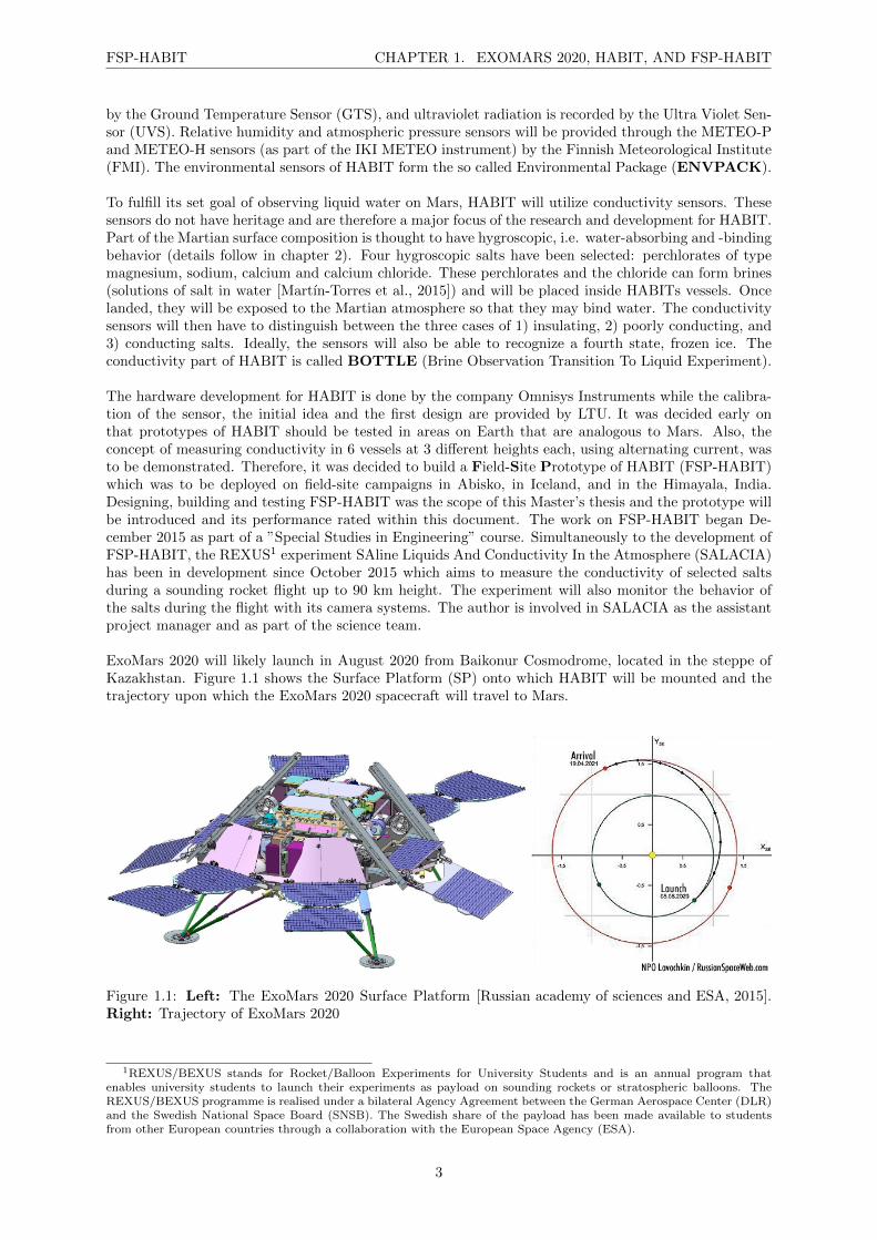
HAbitability, Brines, Irradiation and Temperature (HABIT) has been selected to be part of the Exo-Mars 2020 payload and as such will embark towards Mars in 2020. ExoMars is a joint program by theEuropean Space Agency (ESA) and the Space Research Institute of the Russian Academy of Sciences(IKI) which consists of two missions, in 2016 and 2020. The 2016 mission includes the Trace Gas Orbiter(TGO) and an Entry, Descent and landing Demonstrator (EDM). The 2020 mission will bring the firstEuropean/Russian rover to the surface of Mars and the Surface Platform (SP) will be used to safely landthe rover. The SP will also contain a suite of instruments, including HABIT.
HABIT will be the first Swedish instrument to be deployed on the surface of Mars and is currently underdevelopment by the Lulea University of Technology (LTU) and Omnisys Instruments, both located inSweden. HABIT is a Principal Investigator(PI)-led instrument by PI F. Javier Martın-Torres and Co-PIMaria-Paz Zorzano Mier, both from Lulea University of Technology. It has a suite of sensors chosen tofulfill its specific scientific goals (from HABIT proposal):
To assess the present day habitability of the upper meters of the Martian regolith.
Direct in-situ observation of liquid water production at Martian environmental conditions.
Derivation of the UV irradiation biological dose at the surface and subsurface.
Measurement of the surface temperature diurnal and seasonal range, and derivation of the sub-surface regolith behavior and the windows of time when the regolith can allow for replication andmetabolism.
To provide information about the environment, the water cycle, the dust cycle and climate at theboundary layer.
Derivation of the windows of time when the surface and subsurface allow for frost and/or liquidwater formation, and its role in mineral alteration.
HABIT will also provide critical information for future In-Situ Resource Utilization (ISRU) technologies.In particular the BOTTLE investigation package, which encompasses the salt conductivity experiments,will serve as a demonstrator of ISRU technology. Other goals of HABIT are therefore:
The quantification of the maximal amount of water available for life and future exploration.
In-situ validation of thermal regeneration strategies.
HABIT has heritage as both PI’s were Co-Investigators of the Mars Science Laboratory / Rover Environ-mental Monitoring Station (MSL-REMS) instrument. NASAs MSL, commonly known as the ”Curiosity”rover, has been operating at Gale Crater on Mars since August 2012 and REMS has been recording at-mospheric parameters ever since. HABIT will, together with the Meteorological package (METEO)instrument, monitor the same atmospheric parameters as REMS: Wind speed/direction and air temper-ature will be monitored by the Air Temperature Sensor (ATS), ground temperature will be determined
2
FSP-HABIT CHAPTER 1. EXOMARS 2020, HABIT, AND FSP-HABIT
by the Ground Temperature Sensor (GTS), and ultraviolet radiation is recorded by the Ultra Violet Sen-sor (UVS). Relative humidity and atmospheric pressure sensors will be provided through the METEO-Pand METEO-H sensors (as part of the IKI METEO instrument) by the Finnish Meteorological Institute(FMI). The environmental sensors of HABIT form the so called Environmental Package (ENVPACK).
To fulfill its set goal of observing liquid water on Mars, HABIT will utilize conductivity sensors. Thesesensors do not have heritage and are therefore a major focus of the research and development for HABIT.Part of the Martian surface composition is thought to have hygroscopic, i.e. water-absorbing and -bindingbehavior (details follow in chapter 2). Four hygroscopic salts have been selected: perchlorates of typemagnesium, sodium, calcium and calcium chloride. These perchlorates and the chloride can form brines(solutions of salt in water [Martın-Torres et al., 2015]) and will be placed inside HABITs vessels. Oncelanded, they will be exposed to the Martian atmosphere so that they may bind water. The conductivitysensors will then have to distinguish between the three cases of 1) insulating, 2) poorly conducting, and3) conducting salts. Ideally, the sensors will also be able to recognize a fourth state, frozen ice. Theconductivity part of HABIT is called BOTTLE (Brine Observation Transition To Liquid Experiment).
The hardware development for HABIT is done by the company Omnisys Instruments while the calibra-tion of the sensor, the initial idea and the first design are provided by LTU. It was decided early onthat prototypes of HABIT should be tested in areas on Earth that are analogous to Mars. Also, theconcept of measuring conductivity in 6 vessels at 3 different heights each, using alternating current, wasto be demonstrated. Therefore, it was decided to build a Field-Site Prototype of HABIT (FSP-HABIT)which was to be deployed on field-site campaigns in Abisko, in Iceland, and in the Himayala, India.Designing, building and testing FSP-HABIT was the scope of this Master’s thesis and the prototype willbe introduced and its performance rated within this document. The work on FSP-HABIT began De-cember 2015 as part of a ”Special Studies in Engineering” course. Simultaneously to the development ofFSP-HABIT, the REXUS1 experiment SAline Liquids And Conductivity In the Atmosphere (SALACIA)has been in development since October 2015 which aims to measure the conductivity of selected saltsduring a sounding rocket flight up to 90 km height. The experiment will also monitor the behavior ofthe salts during the flight with its camera systems. The author is involved in SALACIA as the assistantproject manager and as part of the science team.
ExoMars 2020 will likely launch in August 2020 from Baikonur Cosmodrome, located in the steppe ofKazakhstan. Figure 1.1 shows the Surface Platform (SP) onto which HABIT will be mounted and thetrajectory upon which the ExoMars 2020 spacecraft will travel to Mars.
Figure 1.1: Left: The ExoMars 2020 Surface Platform [Russian academy of sciences and ESA, 2015].Right: Trajectory of ExoMars 2020
1REXUS/BEXUS stands for Rocket/Balloon Experiments for University Students and is an annual program thatenables university students to launch their experiments as payload on sounding rockets or stratospheric balloons. TheREXUS/BEXUS programme is realised under a bilateral Agency Agreement between the German Aerospace Center (DLR)and the Swedish National Space Board (SNSB). The Swedish share of the payload has been made available to studentsfrom other European countries through a collaboration with the European Space Agency (ESA).
3

Chapter 2
Scientific Background
Could Mars harbor life? This question has fascinated humanity throughout the ages and we are closerto getting an answer than ever before. The main condition for Earth-type life is the presence of liquidwater [McKay, 2006]. However, typical atmospheric parameters found on the Martian surface should notallow liquid water to exist at all. The Martian average temperature is about 215− 218 K [Catling, 2014]and its pressure is usually found between 4-8.7 mbar [NASA/NSSDC, 2014], depending on the season. Acomparison with the phase diagram of water (figure 2.1) clearly shows that these conditions would onlyallow water as either ice or directly sublimated into water vapor. Since Mars exhibits diurnal temperaturechanges that can be as strong as 90-100 K (e.g. data recorded at Gale crater, [Martın-Torres et al., 2015])during a single Martian day, surface temperatures can range from about 140 to 310 K [Catling, 2014].As can be seen in figure 2.1, the typical Martian conditions provide only an extremely narrow windowwere liquid water could exist. Temperatures above freezing are typically found only in a thin layer atthe interface between the soil and the atmosphere [Catling, 2014]. Since the surface air pressure is belowthe triple point of water over much of the planet, any liquid water would immediately boil away attemperatures above freezing [Catling, 2014].
Figure 2.1: Phase diagram of water. The typical Martian conditions have been marked and are foundbetween 4-8.7 mbar and 140-310 K. Source for diagram: Wikimedia commons
4

FSP-HABIT CHAPTER 2. SCIENTIFIC BACKGROUND
Despite this, recent research by [Martın-Torres et al., 2015] inferred that an active water cycle existson present day Mars. Furthermore, indirect evidence of transient liquid water has been retrievedfrom rover[Martın-Torres et al., 2015], lander [Renno et al., 2009] and orbiter [Ojha et al., 2015]. Geo-chemical data and models support the view that Mars once was warm enough to support widespreadliquid water. However, the data and models further support the view that much of the original atmo-spheric inventory was lost to space long ago. For the last 3.7 billion years, Mars is thought to have beenin a cold and dry state, therefore geologically recent outflow channels must have been formed by fluidrelease mechanisms that do not depend upon a warm climate. This is expected to also be valid for veryrecent gullies and summertime dark lineae that form on steep slopes [Catling, 2014].
Certain types of salt can offer a possible explanation as they show hygroscopic behavior, i.e. they absorbatmospheric water [Ojha et al., 2015]. It is likely that the bound water does not freeze immediatelyas perchlorate salts can lower the freezing point of water [Mohlmann and Thomsen, 2011]. Moreover,perchlorates can form stable hydrated compounds and liquid solutions by absorbing atmospheric watervapour through deliquescence [Nuding et al., 2014a] [Zorzano et al., 2009]. Deliquescence occurs on Marsduring night time when the temperatures are low and the humidity is high [Martın-Torres et al., 2015].Atmospheric parameters monitored by MSL-REMS suggest that deliquescence could occur at Gale craterthroughout a Martian year with the exception of summer, when the temperatures are high and the hu-midity low [Martın-Torres et al., 2015]. Chloride and perchlorate salts are widespread in the regolithof present day Mars. Figure 2.2 shows observations of the Mars Odyssey Gamma Ray Spectrometerwhich detected that chlorine distributions range from 0.2 to 0.8 wt%, with a mean concentration of0.49 wt% over the planet excluding high-latitude regions [Keller et al., 2006]. Wet chemistry analy-sis of Martian soil at the Phoenix landing site showed that perchlorate salts made up 0.4 - 0.6 wt%[Hecht et al., 2009]. The following salts have been indentified to be of interest and were selected forHABIT ([Martın-Torres et al., 2013] and references therein):
Calcium Perchlorate Ca(ClO4)2, Te = 196 K
Magnesium Perchlorate Mg(ClO4)2, Te = 206 K
Calcium Chloride CaCl2, Te = 226 K
Sodium Perchlorate NaClO4, Te = 236 K
The salts are sorted after their eutectic temperature Te. To allow for liquid water, the ambient tempera-ture has to be above the eutectic temperature and, at the same time, the relative humidity must be withina suitable range. Considering the average Martian temperature of Tavg = 215 − 218 K [Catling, 2014],it can be seen that the Te for two of the salts lies below the average.
Figure 2.2: Equatorial and mid-latitude distribution of chlorine within the top 1 meter,measured by Mars Odyssey Gamma Ray Spectrometer. The global concentration of Cl issimilar to the measured concentration of ClO−
4 at the Phoenix and Curiosity landing sites, suggestingthat ClO−
4 could be globally distributed. Credit: [Keller et al., 2006]
5
FSP-HABIT CHAPTER 2. SCIENTIFIC BACKGROUND
2.1 Water On Mars
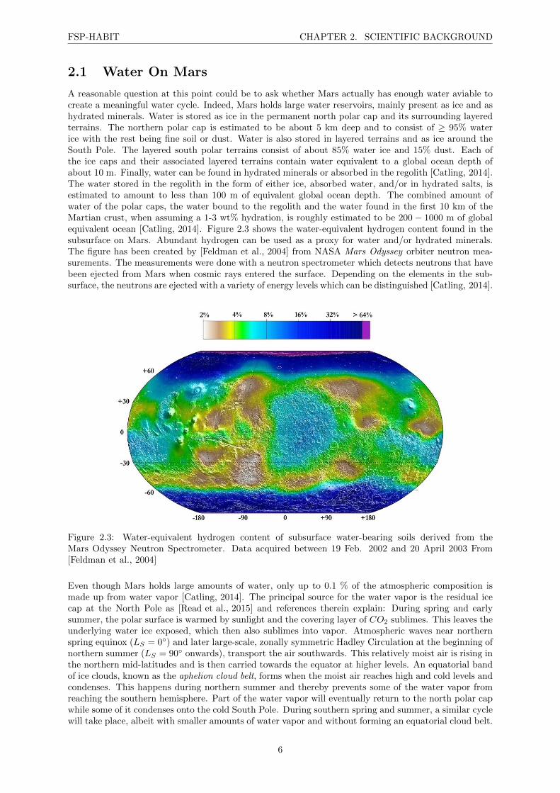
A reasonable question at this point could be to ask whether Mars actually has enough water aviable tocreate a meaningful water cycle. Indeed, Mars holds large water reservoirs, mainly present as ice and ashydrated minerals. Water is stored as ice in the permanent north polar cap and its surrounding layeredterrains. The northern polar cap is estimated to be about 5 km deep and to consist of ≥ 95% waterice with the rest being fine soil or dust. Water is also stored in layered terrains and as ice around theSouth Pole. The layered south polar terrains consist of about 85% water ice and 15% dust. Each ofthe ice caps and their associated layered terrains contain water equivalent to a global ocean depth ofabout 10 m. Finally, water can be found in hydrated minerals or absorbed in the regolith [Catling, 2014].The water stored in the regolith in the form of either ice, absorbed water, and/or in hydrated salts, isestimated to amount to less than 100 m of equivalent global ocean depth. The combined amount ofwater of the polar caps, the water bound to the regolith and the water found in the first 10 km of theMartian crust, when assuming a 1-3 wt% hydration, is roughly estimated to be 200 − 1000 m of globalequivalent ocean [Catling, 2014]. Figure 2.3 shows the water-equivalent hydrogen content found in thesubsurface on Mars. Abundant hydrogen can be used as a proxy for water and/or hydrated minerals.The figure has been created by [Feldman et al., 2004] from NASA Mars Odyssey orbiter neutron mea-surements. The measurements were done with a neutron spectrometer which detects neutrons that havebeen ejected from Mars when cosmic rays entered the surface. Depending on the elements in the sub-surface, the neutrons are ejected with a variety of energy levels which can be distinguished [Catling, 2014].
Figure 2.3: Water-equivalent hydrogen content of subsurface water-bearing soils derived from theMars Odyssey Neutron Spectrometer. Data acquired between 19 Feb. 2002 and 20 April 2003 From[Feldman et al., 2004]
Even though Mars holds large amounts of water, only up to 0.1 % of the atmospheric composition ismade up from water vapor [Catling, 2014]. The principal source for the water vapor is the residual icecap at the North Pole as [Read et al., 2015] and references therein explain: During spring and earlysummer, the polar surface is warmed by sunlight and the covering layer of CO2 sublimes. This leaves theunderlying water ice exposed, which then also sublimes into vapor. Atmospheric waves near northernspring equinox (LS = 0) and later large-scale, zonally symmetric Hadley Circulation at the beginning ofnorthern summer (LS = 90 onwards), transport the air southwards. This relatively moist air is rising inthe northern mid-latitudes and is then carried towards the equator at higher levels. An equatorial bandof ice clouds, known as the aphelion cloud belt, forms when the moist air reaches high and cold levels andcondenses. This happens during northern summer and thereby prevents some of the water vapor fromreaching the southern hemisphere. Part of the water vapor will eventually return to the north polar capwhile some of it condenses onto the cold South Pole. During southern spring and summer, a similar cyclewill take place, albeit with smaller amounts of water vapor and without forming an equatorial cloud belt.
6
FSP-HABIT CHAPTER 2. SCIENTIFIC BACKGROUND
Mars is also closer to the Sun and slightly warmer on average during these seasons. The atmosphericcomposition on present day Mars can be seen in table 2.1.
Constituent Mars EarthCO2 0.953 399.41 ppmN2 0.027 0.7808O2 0.0013 0.2095CH4 <1 ppbv 2 ppmH2O <100 ppm <0.03Ar 0.016 0.009CO 700 ppm 0.2 ppmO3 0.01 ppm 10 ppm
Table 2.1: Atmospheric compositions of Mars and Earth. Adapted from [de Pater and Lissauer, 2013];the CO2-value for Earth is from [NOAA ESRL/GMD, 2015]; The CH4-value for Mars is from[Catling, 2014] and references therein.
2.1.1 Relative Humidity (RH)
A major factor for the creation of brines is the available atmospheric water vapor on the atmosphere-surface interface. The absolute amount of water in the ambient air is typically expressed through thevolume mixing ratio (VMR), given in ppm (parts per million) while the amount of water currently heldby the air as compared to the amount of water the air could hold at maximal saturation is expressed asrelative humidity (RH), given in %. Relative humidity is defined by
RH =e
eS(T )(2.1)
where e is the partial pressure of water vapor, related to the VMR by
VMR =e
p(2.2)
with p being the total air pressure. The saturation pressure eS(T ) is given by
eS(T ) = eS(T0)expL
RV
( 1
T0− 1
T
)(2.3)
where L is the the latent heat of vaporization per unit mass (also called the specific enthalpy of vapor-ization), given by L = TδS, with S being the entropy. RV is the specific gas constant for the vapor, T0is a constant reference temperature, and T is the ambient temperature [Andrews, 2010].
Measurements by the REMS-H sensor on board MSL recorded the relative humidity for a whole Mar-tian year (about 2 Earth years). Figure 2.4 shows the diurnal maximum RH-values from LS = 0 toLS = 360 at Gale crater (4.6S, 137.4E, at 4.5 km below the datum). These maxima are usuallyrecorded in the early morning prior to sunrise when the air temperatures reach their minimum. HereLS = 90 (winter), LS = 180 (spring), LS = 270 (summer) and LS = 360 = 0 (autumn). RHmax
a , dottedin blue, has been recorded by REMS-H which is mounted to the MSL camera mast at 1.6 m height.As can be seen, the relative humidity is maximized at the beginning of winter and is anti-correlatedwith the ambient temperature [Martın-Torres et al., 2015]. After two years, a smooth transition can beseen between LS = 360 and LS = 0, increasing the confidence in the measured data. The values forthe surface RHmax
g have been calculated by evaluating the temperatures recorded by the IR groundtemperature sensor [Martın-Torres et al., 2015]. According to the calculated values, the maximum rel-ative humidity on the ground reaches saturation for half of the Martian year. This finding has beendeemed especially meaningful since Gale crater is located at the equator which marks the driest andwarmest region on the planet. The environmental conditions allow for transiently stable liquid brinesand define a threshold condition for their presence [Martın-Torres et al., 2015]. The scattered variationsfor RHmax
g are due to differing thermal properties of the 8 km of soil that has been explored by the rover.
7

FSP-HABIT CHAPTER 2. SCIENTIFIC BACKGROUND
Figure 2.4: Left: Relative Humidity seasonal behavior. Right: The diurnal RHg and Tg cycle duringsol 551 (LS = 93). Notably, both parameters are anti-correlated with each other. Both figures from[Martın-Torres et al., 2015] supplementary material.
2.2 The Water-Chlorine Correlation
Prior to the inferring of a chloride- and perchlorate-driven water cycle by [Martın-Torres et al., 2015], acorrelation between the distribution of chlorine (Cl) and hydrogen has been noted by [Boynton et al., 2007].As visible in figure 2.5, a similarity is found among the patterns in the maps of Cl and H2O distribu-tions. Both maps show enrichments in Arabia Terra and near Apollinaris Patera while the most obviousdifference between the two is found at Medusae Fossae. Here, a significant enrichment of Cl can benoted while no such increase in H2O is found. [Boynton et al., 2007] stated that this observation pointsto a different source of Cl for the Medusae Fossae Formation than for the rest of Mars where H2O andCl are highly correlated. This extra enrichment is suspected to be due to volcanism associated withthe Tharsis Montes. At the time, the researchers concluded that the close relationship between Cl andH2O in other areas was probably caused by a weathering-related process, suggesting that both elementsmoved together.
Figure 2.5: Top: Map of Cl concentrations and their uncertainties in the low and mid latitudes of Mars.Bottom: Map of H2O concentrations and their uncertainties in the low and mid latitudes of Mars.Both: Data acquired between 8 Jun. 2002 and 2 April 2005 From [Boynton et al., 2007]
[Keller et al., 2006] and references therein proposed mechanisms which could account for the enrichmentof Cl at the surface. They include: volatile release associated with volcanic activity, chemical weatheringof igneous rocks, and concentration through the processes of water transport, hydrothermal alterationevaporation, and wind. [Keller et al., 2006] reported a positive correlation of Cl with H, a negative
8
FSP-HABIT CHAPTER 2. SCIENTIFIC BACKGROUND
correlation of Cl with Si, and a less pronounced negative correlation of Cl with thermal inertia. Together,these three correlations account to about 40 % of the variation seen in the analyzed Cl data set.
2.3 Brines And Transient Liquid Water
As stated previously, the pressure found on present day Mars is of the same magnitude as the pressureat the triple point of water (about 6 mbar). Therefore, liquid water would be theoretically possiblein regions with higher pressure than the triple point. Due to low surface temperatures, however, thepresence of pure liquid water is inhibit even in the lowest regions of Mars such as the Phoenix landingsite (7-8 mbar, 180-250 K) [Renno et al., 2009]. Nonetheless, observations of possible evidence for liquidwater have been made on several occasions. [Renno et al., 2009] reported spheroid structures, behavingsimilar to water droplets, on one of the struts of the Phoenix lander. These spheriods are thought tohave been created after the touchdown of the Phoenix lander when the hot plumes of the hydrazinecombustion engines removed the topsoil, exposed the subsurface ice, and splashed sticky brines onto thelanding struts. The brines would then bind water to themselves through deliquescence over the timescaleof a few days. Other reports of transient liquid water include the already mentioned observations fromrover[Martın-Torres et al., 2015], lander [Renno et al., 2009] and orbiter [Ojha et al., 2015]. All publica-tions have in common that they consider brines (solutions of salt in water) to be possible explanationsfor the observed phenomena.
As evaluated by [Renno et al., 2009] and references therein, many salts depress the freezing temperatureand by doing so could enable the existence of liquid saline water below water freezing temperatures. Also,by depressing the freezing point temperature, the salts reduce the vapor pressure of aqueous solutions,lowering their boiling point pressure. Salts are deliquescent materials which absorb water when exposedto the atmosphere, and form liquid solutions when the relative humidity is above a threshold valueknown as the deliquescence relative humidity, RHD. These solutions usually remain liquid until therelative humidity falls below a much lower value known as the efflorescence relative humidity, RHEF
[Seinfeld and Pandis, 2006].
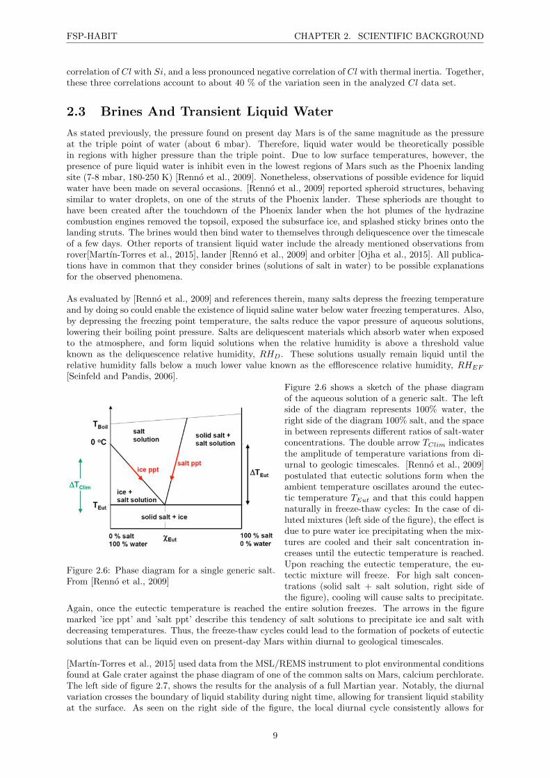
Figure 2.6: Phase diagram for a single generic salt.From [Renno et al., 2009]
Figure 2.6 shows a sketch of the phase diagramof the aqueous solution of a generic salt. The leftside of the diagram represents 100% water, theright side of the diagram 100% salt, and the spacein between represents different ratios of salt-waterconcentrations. The double arrow TClim indicatesthe amplitude of temperature variations from di-urnal to geologic timescales. [Renno et al., 2009]postulated that eutectic solutions form when theambient temperature oscillates around the eutec-tic temperature TEut and that this could happennaturally in freeze-thaw cycles: In the case of di-luted mixtures (left side of the figure), the effect isdue to pure water ice precipitating when the mix-tures are cooled and their salt concentration in-creases until the eutectic temperature is reached.Upon reaching the eutectic temperature, the eu-tectic mixture will freeze. For high salt concen-trations (solid salt + salt solution, right side ofthe figure), cooling will cause salts to precipitate.
Again, once the eutectic temperature is reached the entire solution freezes. The arrows in the figuremarked ’ice ppt’ and ’salt ppt’ describe this tendency of salt solutions to precipitate ice and salt withdecreasing temperatures. Thus, the freeze-thaw cycles could lead to the formation of pockets of eutecticsolutions that can be liquid even on present-day Mars within diurnal to geological timescales.
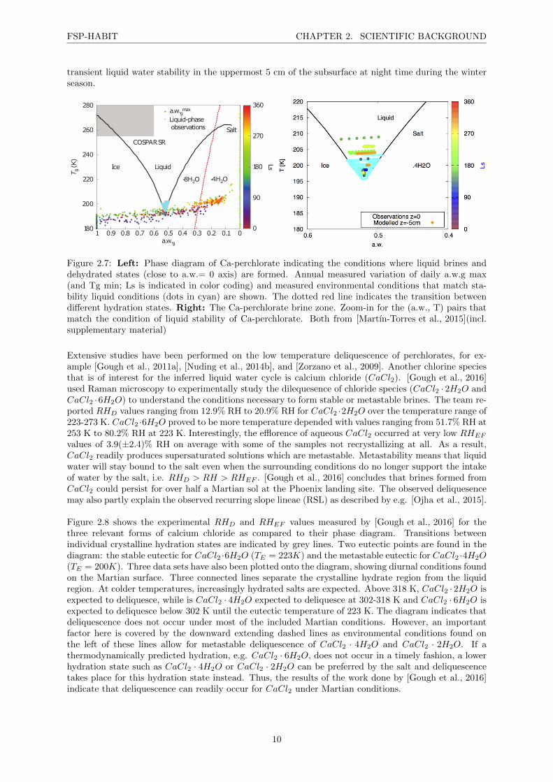
[Martın-Torres et al., 2015] used data from the MSL/REMS instrument to plot environmental conditionsfound at Gale crater against the phase diagram of one of the common salts on Mars, calcium perchlorate.The left side of figure 2.7, shows the results for the analysis of a full Martian year. Notably, the diurnalvariation crosses the boundary of liquid stability during night time, allowing for transient liquid stabilityat the surface. As seen on the right side of the figure, the local diurnal cycle consistently allows for
9
FSP-HABIT CHAPTER 2. SCIENTIFIC BACKGROUND
transient liquid water stability in the uppermost 5 cm of the subsurface at night time during the winterseason.
180
200
220
240
260
280
00.10.20.30.40.50.60.70.80.91a.w.g
LiquidIce
Salt
⋅8H2O ⋅4H2O
COSPAR SR
a.w.gmax
Liquid-phase observations
0
90
180
270
360
Ls
T g(K
)
Figure 2.7: Left: Phase diagram of Ca-perchlorate indicating the conditions where liquid brines anddehydrated states (close to a.w.= 0 axis) are formed. Annual measured variation of daily a.w.g max(and Tg min; Ls is indicated in color coding) and measured environmental conditions that match sta-bility liquid conditions (dots in cyan) are shown. The dotted red line indicates the transition betweendifferent hydration states. Right: The Ca-perchlorate brine zone. Zoom-in for the (a.w., T) pairs thatmatch the condition of liquid stability of Ca-perchlorate. Both from [Martın-Torres et al., 2015](incl.supplementary material)
Extensive studies have been performed on the low temperature deliquescence of perchlorates, for ex-ample [Gough et al., 2011a], [Nuding et al., 2014b], and [Zorzano et al., 2009]. Another chlorine speciesthat is of interest for the inferred liquid water cycle is calcium chloride (CaCl2). [Gough et al., 2016]used Raman microscopy to experimentally study the dilequesence of chloride species (CaCl2 · 2H2O andCaCl2 ·6H2O) to understand the conditions necessary to form stable or metastable brines. The team re-ported RHD values ranging from 12.9% RH to 20.9% RH for CaCl2 ·2H2O over the temperature range of223-273 K. CaCl2 ·6H2O proved to be more temperature depended with values ranging from 51.7% RH at253 K to 80.2% RH at 223 K. Interestingly, the efflorence of aqueous CaCl2 occurred at very low RHEF
values of 3.9(±2.4)% RH on average with some of the samples not recrystallizing at all. As a result,CaCl2 readily produces supersaturated solutions which are metastable. Metastability means that liquidwater will stay bound to the salt even when the surrounding conditions do no longer support the intakeof water by the salt, i.e. RHD > RH > RHEF . [Gough et al., 2016] concludes that brines formed fromCaCl2 could persist for over half a Martian sol at the Phoenix landing site. The observed deliquesencemay also partly explain the observed recurring slope lineae (RSL) as described by e.g. [Ojha et al., 2015].
Figure 2.8 shows the experimental RHD and RHEF values measured by [Gough et al., 2016] for thethree relevant forms of calcium chloride as compared to their phase diagram. Transitions betweenindividual crystalline hydration states are indicated by grey lines. Two eutectic points are found in thediagram: the stable eutectic for CaCl2 ·6H2O (TE = 223K) and the metastable eutectic for CaCl2 ·4H2O(TE = 200K). Three data sets have also been plotted onto the diagram, showing diurnal conditions foundon the Martian surface. Three connected lines separate the crystalline hydrate region from the liquidregion. At colder temperatures, increasingly hydrated salts are expected. Above 318 K, CaCl2 · 2H2O isexpected to deliquesce, while is CaCl2 · 4H2O expected to deliquesce at 302-318 K and CaCl2 · 6H2O isexpected to deliquesce below 302 K until the eutectic temperature of 223 K. The diagram indicates thatdeliquescence does not occur under most of the included Martian conditions. However, an importantfactor here is covered by the downward extending dashed lines as environmental conditions found onthe left of these lines allow for metastable deliquescence of CaCl2 · 4H2O and CaCl2 · 2H2O. If athermodynamically predicted hydration, e.g. CaCl2 · 6H2O, does not occur in a timely fashion, a lowerhydration state such as CaCl2 · 4H2O or CaCl2 · 2H2O can be preferred by the salt and deliquescencetakes place for this hydration state instead. Thus, the results of the work done by [Gough et al., 2016]indicate that deliquescence can readily occur for CaCl2 under Martian conditions.
10

FSP-HABIT CHAPTER 2. SCIENTIFIC BACKGROUND
Figure 2.8: Phase diagram for different hydration states of CaCl2. The RHD and RHEF values attainedthrough experimentation are overlaid onto the theoretical phase transition boundaries (stable: solid lines;metastable: dashed lines). From [Gough et al., 2016]
2.4 Conductivity
Salts are electrolytes and as such can conduct when in contact with water [EMERSON, 2010]. Elec-trical conductivity is directly linked to the electrical resistivity which is a key physical property of anygiven material and indicates how well the current is transmitted. As [Heaney, 2004] explains, electricalresistivity ρ is the inverse of the electrical conductivity σ with:
σ ≡ 1
ρ(2.4)
As the resistivity ρ describes how strongly a given material opposes the flow of electric current, it can bedefined as a proportionality coefficient which relates a local applied electric field to the resultant currentdensity:
E ≡ ρJ (2.5)
where E is the electric field [V/m] and J is the current density [A/m2]. Both E and J are vectors whileρ is generally a tensor. However, when the material under test is isotropic and homogeneous, ρ becomesa scalar. If one considers a bar-shaped sample with a length l, the electric field E is given by
E ≡ V
l(2.6)
where V is the voltage over the sample. Combining equation 2.5 and equation 2.6, with the equation forthe current density,
J ≡ I
A(2.7)
where I is the current and A is the cross sectional area of the sample, gives:
V =Iρl
A= I · ρ ·K (2.8)
where K is the so called cell constant, given in [cm−1]. Together with the resistance R, given by
R ≡ ρl
A≡ ρ ·K (2.9)
one arrives at Ohm’s law:
I =V
R(2.10)
11
FSP-HABIT CHAPTER 2. SCIENTIFIC BACKGROUND
Another commonly used quantity is the electrical conductance which is defined as the reciprocal of theelectrical resistance R of a salty solution between two electrodes in FSP-HABIT’s case. [Analytical, 2004]states that:
G =1
R(2.11)
with G being given in the unit Siemens [1 S]. The conductivity of a salty solution can then be calculatedby
σ = G ·K (2.12)
and the conductivity σ is given in [S/m].
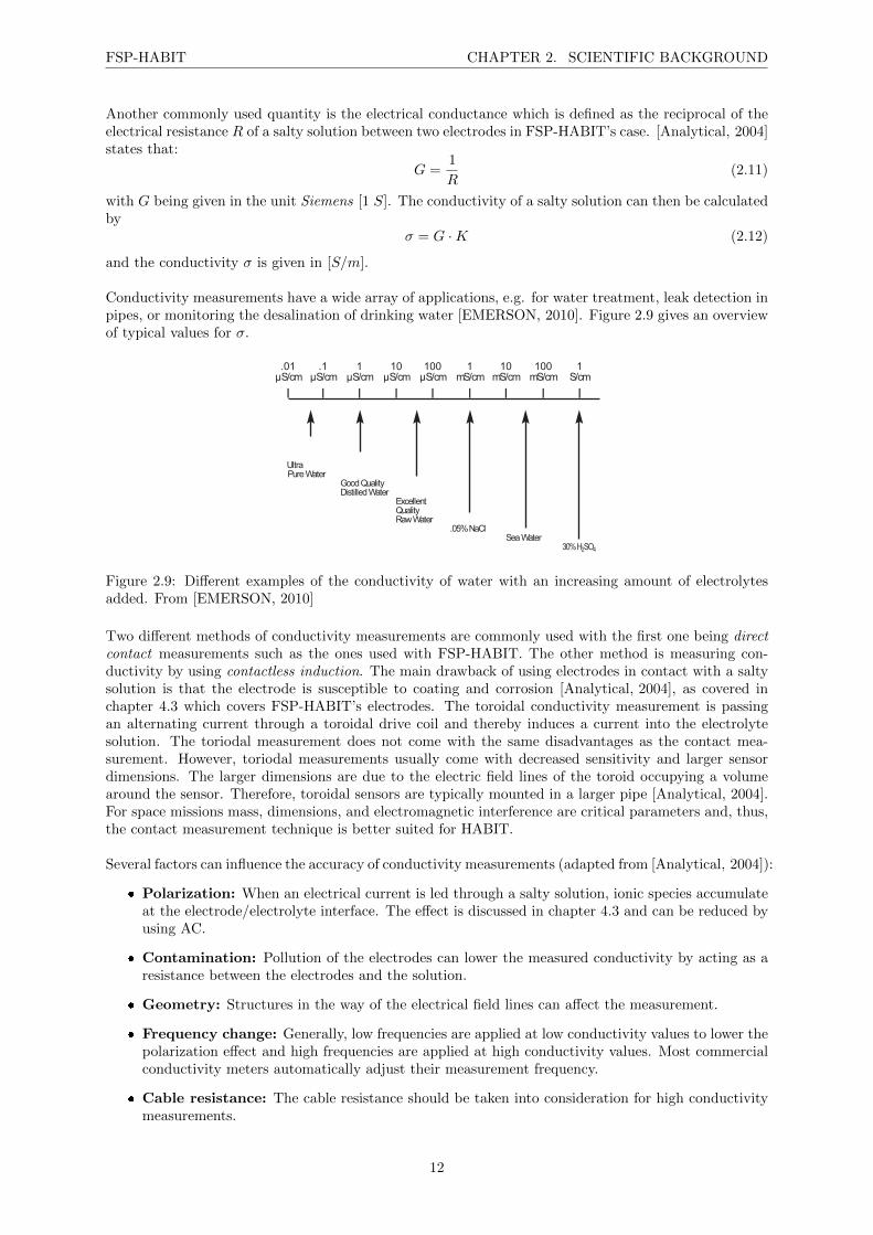
Conductivity measurements have a wide array of applications, e.g. for water treatment, leak detection inpipes, or monitoring the desalination of drinking water [EMERSON, 2010]. Figure 2.9 gives an overviewof typical values for σ.
.01 .1 1 10 100 1 10 100 1µS/cm µS/cm µS/cm µS/cm µS/cm mS/cm mS/cm mS/cm S/cm
I I I I I I I I I
UltraPureWater
GoodQualityDistilledWater
ExcellentQualityRawWater
.05%NaClSeaWater
30%H2SO4
Figure 2.9: Different examples of the conductivity of water with an increasing amount of electrolytesadded. From [EMERSON, 2010]
Two different methods of conductivity measurements are commonly used with the first one being directcontact measurements such as the ones used with FSP-HABIT. The other method is measuring con-ductivity by using contactless induction. The main drawback of using electrodes in contact with a saltysolution is that the electrode is susceptible to coating and corrosion [Analytical, 2004], as covered inchapter 4.3 which covers FSP-HABIT’s electrodes. The toroidal conductivity measurement is passingan alternating current through a toroidal drive coil and thereby induces a current into the electrolytesolution. The toriodal measurement does not come with the same disadvantages as the contact mea-surement. However, toriodal measurements usually come with decreased sensitivity and larger sensordimensions. The larger dimensions are due to the electric field lines of the toroid occupying a volumearound the sensor. Therefore, toroidal sensors are typically mounted in a larger pipe [Analytical, 2004].For space missions mass, dimensions, and electromagnetic interference are critical parameters and, thus,the contact measurement technique is better suited for HABIT.
Several factors can influence the accuracy of conductivity measurements (adapted from [Analytical, 2004]):
Polarization: When an electrical current is led through a salty solution, ionic species accumulateat the electrode/electrolyte interface. The effect is discussed in chapter 4.3 and can be reduced byusing AC.
Contamination: Pollution of the electrodes can lower the measured conductivity by acting as aresistance between the electrodes and the solution.
Geometry: Structures in the way of the electrical field lines can affect the measurement.
Frequency change: Generally, low frequencies are applied at low conductivity values to lower thepolarization effect and high frequencies are applied at high conductivity values. Most commercialconductivity meters automatically adjust their measurement frequency.
Cable resistance: The cable resistance should be taken into consideration for high conductivitymeasurements.
12
FSP-HABIT CHAPTER 2. SCIENTIFIC BACKGROUND
Cable capacitance: Shielded cables with a given length have some capacity. The measurementshould be compensated when measuring low conductivity values.
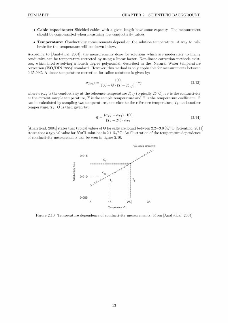
Temperature: Conductivity measurements depend on the solution temperature. A way to cali-brate for the temperature will be shown below.
According to [Analytical, 2004], the measurements done for solutions which are moderately to highlyconductive can be temperature corrected by using a linear factor. Non-linear correction methods exist,too, which involve solving a fourth degree polynomial, described in the ’Natural Water temperaturecorrection (ISO/DIN 7888)’ standard. However, this method is only applicable for measurements between0-35.9C. A linear temperature correction for saline solutions is given by:
σTref =100
100 + Θ · (T − Tref )· σT (2.13)
where σTref is the conductivity at the reference temperature Tref (typically 25C), σT is the conductivityat the current sample temperature, T is the sample temperature and Θ is the temperature coefficient. Θcan be calculated by sampling two temperatures, one close to the reference temperature, T1, and anothertemperature, T2. Θ is then given by:
Θ =(σT2 − σT1) · 100
(T2 − T1) · σT1(2.14)
[Analytical, 2004] states that typical values of Θ for salts are found between 2.2−3.0 %/C. [Scientific, 2011]states that a typical value for NaCl-solutions is 2.1 %/C. An illustration of the temperature dependenceof conductivity measurements can be seen in figure 2.10.
0.005
0.010
0.015
Con
duct
ivity
S/c
m
Temperature ˚C
5 15 25 35
Real sample conductivity
T2
T1
ΚT1
ΚT2
Figure 2.10: Temperature dependence of conductivity measurements. From [Analytical, 2004]
13

Chapter 3
Instrument Overview
The goal of this thesis was to design and build a portable prototype where several sensors are connectedto an ARDUINO to get the sensor readings and to save them to a data storage device. This includeddefining the basic setup, acquiring the components and implementing at least 1 of them with success.It further included the mechanical configuration/batteries and data-saving/sending protocols that maybe required for operation outdoors. The measurements, uncertainties and sources of errors were to beanalyzed in the context of the science objectives of the HABIT instrument for the Surface Platform ofExoMars.
As explained in the disclosure, the rest of this chapter has already been used in another report for thesubject ”Special Studies in Engineering” and is included in this thesis as it gives a good overview of theinitial goals for the prototype.
3.1 Mission Statement
Chloride and perchlorate salts are widely distributed on Mars. Their hygroscopic behavior has beenstudied thoroughly under laboratory conditions and has been correlated to data from Mars and Earthbased measurements. This field-site prototype will now enable scientists to directly study the behaviorof these salts in-situ in cold, arid, and dry environments on Earth. The results can then be compared toother on-going research, e.g. the study of perchlorate salts in the Atacama desert [H. N. Farris, 2016].The prototype will further act as a demonstrator for the upcoming HABIT instrument which will testthe salts on the Martian surface.
3.2 Instrument Objectives
FSP-HABIT has the following primary objectives:
1. Measure the changes in conductivity of selected brines (solutions of water in salt) when subjectedto ambient conditions of cold and dry environments on Earth. The selected brines stem from thefollowing salts which are commonly found on Mars:
1.1. Magnesium Perchlorate Mg(ClO4)2
1.2. Sodium Perchlorate NaClO4
1.3. Calcium Perchlorate Ca(ClO4)2
1.4. Calcium Chloride CaCl2
2. Measure environmental parameters to quantify the changes in conductivity:
2.1. air temperature at three points such that a hotter object in the instruments field of view canbe detected
2.2. ground temperature
2.3. ambient air pressure
2.4. Relative Humidity (RH)
14

FSP-HABIT CHAPTER 3. INSTRUMENT OVERVIEW
3. Do all of the above autonomously, with an own, re-chargeable, power source
Apart from that, the following secondary objective has been identified for FSP-HABIT:
1. Establish connection to the cellular network such that remote operation and data retrieval arepossible
3.3 Instrument Concept
FSP-HABIT will consist of two main parts. The Brines Container Assembly (BCA) will include thebrines container and corresponding conductivity sensors (at least one per vessel), an air pressure, relativehumidity (RH) and temperature sensor, and a remote temperature sensor for the ground temperature.The ambient RH can be converted with the ambient pressure, air and surface temperature, into surfaceRH, and this will permit to extrapolate the conditions expected on the soil surface without direct contact.This set-up will mimic sensors to be implemented on the Surface Platform in HABIT’s ENVPACK andalso include the relative humidity and pressure sensors provided by METEO-H and METEO-P. TheUV irradiance will be monitored independently since this experiment is focused on validating if thecontainer and surface soil can permit the formation of transient liquid water due to deliquescence. TheElectronics Box assembly (EBox) will be physically separated from the BCA to reduce thermalemissions of the included electronics influencing the conductivity measurements of the brine behavior.The electronics box assembly will contain the ARDUINO as a controlling unit and a battery for power.It will also contain a data storage device and a GSM solution (if the secondary objective is to be fulfilled)which works together with an antenna to connect to a remote station. The concept of FSP-HABIT canbe seen in figure 3.1.
ARDUINOBatteryBrine Container 6
32
1Conductivity
Sensor 1ConductivitySensor 2Conductivity
Sensor 3
ATS 1
ATS 2
ATS 3
RH
GTS
Brines containerassembly
RemoteControl
Telefónica orGSM Shield
solution
Electronics boxassembly
Environmental Sensors
Data Storage
Antenna Pressure
4
5
Figure 3.1: The FSP-HABIT block diagram. ATS - Air Temperature Sensor; GTS - Ground TemperatureSensor; RH - Relative Humidity Sensor
15

Part II
INSTRUMENT DESCRIPTION
17

Chapter 4
Mechanical Design
The mechanical design of FSP-HABIT can be broadly divided into two parts: the brines containerassembly (BCA) and the electronics box assembly (EBox). The idea was to physically separatethe two parts in order to thermally decouple the tested salts from the electronics that would generateheat and therefore alter the experiment outcome. Connecting screws would then hold the two partstogether. The brines container assembly was the first part to be developed and has been the main focuswhile the EBox was done several weeks prior to FSP-HABITs first deployment in Iceland.
4.1 Brines Container Assembly (BCA) Overview
Figure 4.1: Brines ContainerAssembly (BCA) overview
The brines container assembly fulfills several functions: 1)Store salts in six vessels and protect them from contami-nation through dust or other particles. 2) Allow for airto flow freely over the salts so that atmospheric water va-por can be absorbed by them. 3) Provide protrusions forthe three air temperature sensors so that they are thermallydecoupled from the rest of the assembly. 4) Incorporatethe electrodes so that they are in direct contact with thesalts. Figure 4.1 shows the brines container assembly of FSP-HABIT. From top to bottom: Lid, filter fixation, filter mount,brines container, cable canal and air temperature sensor (ATS)mount.
Lid: The lid has the double function of keeping the salt ves-sels save from the surrounding weather (e.g. rain, strong winds)while permitting air to flow freely over the salt vessel filtersthrough gaps of 3 mm between the lid and the filter fixa-tion.
Filter fixation: The fixation will press the filter onto the filter mount,keeping the filter in place. The fixation has eight cutouts which, to-gether with eight brackets from the filter holder, will aid in the assem-bly.
Filter mount: The 0.2 µm filter will be placed onto the filter mount.A grating will provide mechanical stability to the otherwise fragile fil-ter.
Brines container: the container holds the five salt vessels and the ref-erence vessel. Each vessel has electrodes at three measurement heights,as discussed in chapter 4.3. The volume of each vessel is about 9 cm3
and will be covered by the 0.2 µm membrane filter. Towards the out-side walls, twelve pockets (two per brine vessel) are found which doubleas electrode mounts and cable canals. They allow for quick and easy
18
FSP-HABIT CHAPTER 4. MECHANICAL DESIGN
replacement of the electrodes in case of corrosion and protect the wires, which lead from the electrodestowards the electronics box assembly, from changing environmental conditions. Six mounting spots allowfor screws to connect the brines container with the other parts of the brines container assembly. Nearthe open reference vessel of the brines container, two mounting spots are used to connect the BCA withthe EBox.
Cable canal and ATS mount: Used to protect cables from the environment and provides protrusionsfor the Air Temperature Sensor (ATS). The ATS protrusions are used to measure the air temperature ata distance of 40.0 mm from the rest of the BCA and thus reduce the thermal impact on the temperaturesensors. The Pt1000 temperature sensors have been placed at the end of the sticks and glued in place.
4.2 Brines Container Assembly (BCA) Detail
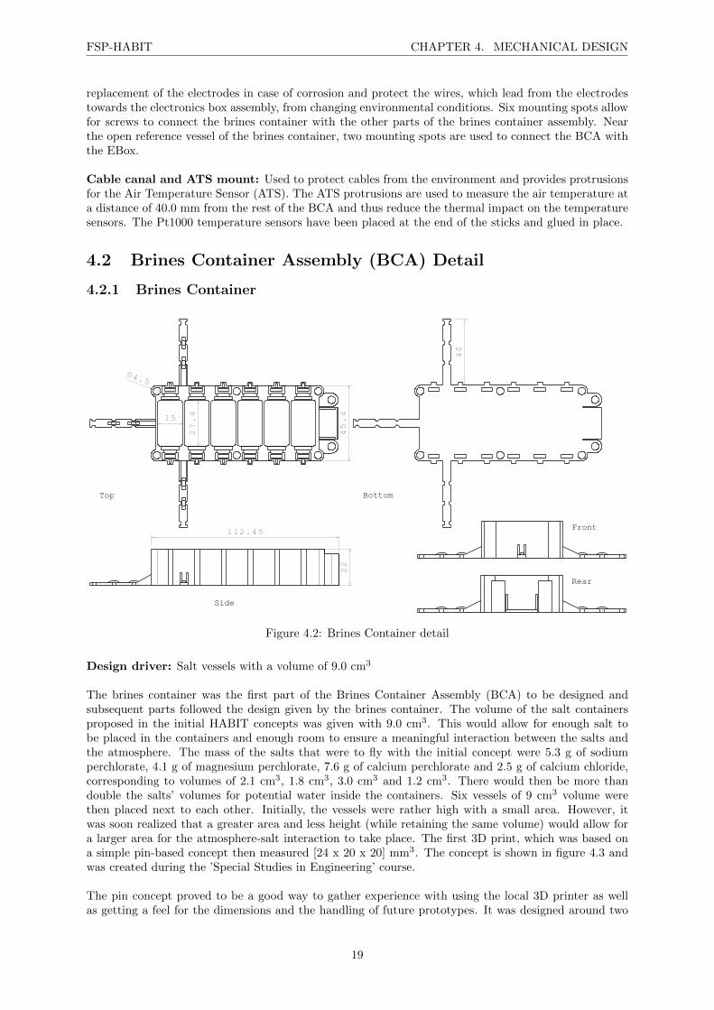
4.2.1 Brines Container
15
Top
27.4
45.4
4 .5
Bottom
40
Side
22
112.45 Front
Rear
Figure 4.2: Brines Container detail
Design driver: Salt vessels with a volume of 9.0 cm3
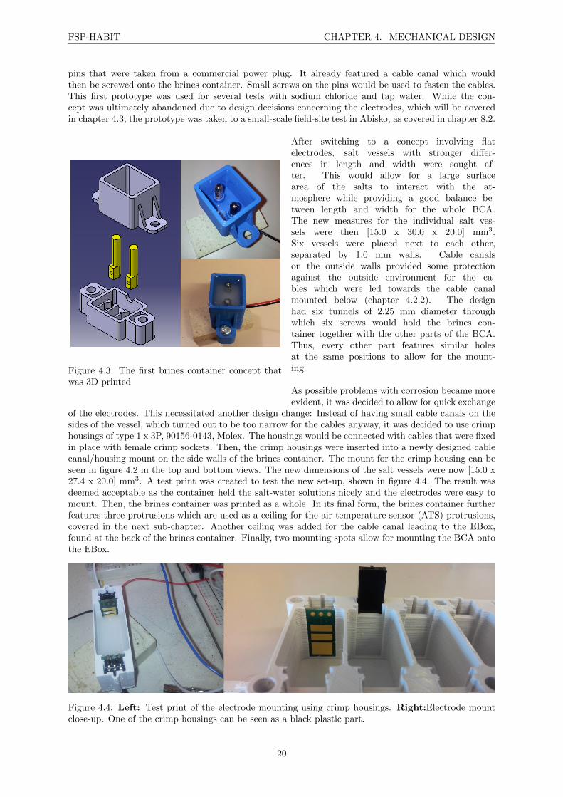
The brines container was the first part of the Brines Container Assembly (BCA) to be designed andsubsequent parts followed the design given by the brines container. The volume of the salt containersproposed in the initial HABIT concepts was given with 9.0 cm3. This would allow for enough salt tobe placed in the containers and enough room to ensure a meaningful interaction between the salts andthe atmosphere. The mass of the salts that were to fly with the initial concept were 5.3 g of sodiumperchlorate, 4.1 g of magnesium perchlorate, 7.6 g of calcium perchlorate and 2.5 g of calcium chloride,corresponding to volumes of 2.1 cm3, 1.8 cm3, 3.0 cm3 and 1.2 cm3. There would then be more thandouble the salts’ volumes for potential water inside the containers. Six vessels of 9 cm3 volume werethen placed next to each other. Initially, the vessels were rather high with a small area. However, itwas soon realized that a greater area and less height (while retaining the same volume) would allow fora larger area for the atmosphere-salt interaction to take place. The first 3D print, which was based ona simple pin-based concept then measured [24 x 20 x 20] mm3. The concept is shown in figure 4.3 andwas created during the ’Special Studies in Engineering’ course.
The pin concept proved to be a good way to gather experience with using the local 3D printer as wellas getting a feel for the dimensions and the handling of future prototypes. It was designed around two
19
FSP-HABIT CHAPTER 4. MECHANICAL DESIGN
pins that were taken from a commercial power plug. It already featured a cable canal which wouldthen be screwed onto the brines container. Small screws on the pins would be used to fasten the cables.This first prototype was used for several tests with sodium chloride and tap water. While the con-cept was ultimately abandoned due to design decisions concerning the electrodes, which will be coveredin chapter 4.3, the prototype was taken to a small-scale field-site test in Abisko, as covered in chapter 8.2.
Figure 4.3: The first brines container concept thatwas 3D printed
After switching to a concept involving flatelectrodes, salt vessels with stronger differ-ences in length and width were sought af-ter. This would allow for a large surfacearea of the salts to interact with the at-mosphere while providing a good balance be-tween length and width for the whole BCA.The new measures for the individual salt ves-sels were then [15.0 x 30.0 x 20.0] mm3.Six vessels were placed next to each other,separated by 1.0 mm walls. Cable canalson the outside walls provided some protectionagainst the outside environment for the ca-bles which were led towards the cable canalmounted below (chapter 4.2.2). The designhad six tunnels of 2.25 mm diameter throughwhich six screws would hold the brines con-tainer together with the other parts of the BCA.Thus, every other part features similar holesat the same positions to allow for the mount-ing.
As possible problems with corrosion became moreevident, it was decided to allow for quick exchange
of the electrodes. This necessitated another design change: Instead of having small cable canals on thesides of the vessel, which turned out to be too narrow for the cables anyway, it was decided to use crimphousings of type 1 x 3P, 90156-0143, Molex. The housings would be connected with cables that were fixedin place with female crimp sockets. Then, the crimp housings were inserted into a newly designed cablecanal/housing mount on the side walls of the brines container. The mount for the crimp housing can beseen in figure 4.2 in the top and bottom views. The new dimensions of the salt vessels were now [15.0 x27.4 x 20.0] mm3. A test print was created to test the new set-up, shown in figure 4.4. The result wasdeemed acceptable as the container held the salt-water solutions nicely and the electrodes were easy tomount. Then, the brines container was printed as a whole. In its final form, the brines container furtherfeatures three protrusions which are used as a ceiling for the air temperature sensor (ATS) protrusions,covered in the next sub-chapter. Another ceiling was added for the cable canal leading to the EBox,found at the back of the brines container. Finally, two mounting spots allow for mounting the BCA ontothe EBox.
Figure 4.4: Left: Test print of the electrode mounting using crimp housings. Right:Electrode mountclose-up. One of the crimp housings can be seen as a black plastic part.
20

FSP-HABIT CHAPTER 4. MECHANICAL DESIGN
4.2.2 Cable Canal And ATS Mount (CCAM)
4.5
Top
45.4
Bottom
40
FrontSide
6112.45
Rear
Figure 4.5: Cable Canal and ATS Mount detail
Design driver: Storage of cables; 40.0 mm protrusions for air temperature sensors
The Cable Canal and ATS Mount (CCAM) has two functions: First, to provide room to lead the cablescoming from the electrode mounts in the brines container towards the EBox while providing some pro-tection from the outside environment. Second, to mount Pt1000 temperature sensors at the tips of thethree protrusions, keeping the temperature sensors 40.0 mm away from the rest of the BCA. This is doneto thermally decouple the sensors from the main body. The CCAM is connected to the brines containervia six screws, just like the rest of the BCA parts. Twelve supports in the middle of the CCAM werethought to be used for some simple cable management and to provide mechanical stability for the brinescontainer. When assembling FSP-HABIT, however, it became clear that they were more in the way ofthe cables than anticipated and that the brines container was stable enough without the supports. Thiswas especially true since the cables just so fit into the CCAM and very little spare room was presentbetween the brines container and the cable canal floor. Therefore, the supports were printed but thenlater removed with a grinding tool.
The ATS Mount was originally planned as separate pins that would be glued to the Cable Canal. Adesign was created that would be placed onto much shorter protrusions on the Cable Canal. An issuewith this approach was that the protrusions would then come with larger dimensions than with theincluded approach. Further, the precision of the 3D-printer would not be high enough to create partsthat then could be seamlessly pushed together so that the protrusions could be unplugged and stowedaway for transport. Printing the protrusions directly with the Cable Canal made the dimensions ofthe protrusions smaller and would mean that three parts less would needed to be printed. Six smallhalf-cylinders per protrusion span the protrusions of the brines container, which comes with respectivecut-outs, to them, creating a tight fit held in place by tension. Finally, the CCAM has a cable outlet atthe back that is covered on top by the brines container. From this spot, the cables are let into the EBox.
21

FSP-HABIT CHAPTER 4. MECHANICAL DESIGN
4.2.3 Filter Fixation And Mount, Filters
Filter Fixation
45.4
27.41 5
Filter Mount
Filter Mount and Fixation Side
2
Filter Mount andFixation Front
Filter Mount andFixation Rear
2 103.9
Figure 4.6: Filter Mount and Fixation detail
Design driver: Mounting thin, exchangeable, filters.
A small membrane filter with a pore size of 0.2 µm has been used for FSP-HABIT. Using membranefilters with a 0.2 µm or smaller pore size was recommended by Gerhard Kminek, an ESA planetaryprotection officer via Petra Rettberg, lead of the Astrobiology Group of the Institute of AerospaceMedicine, integrated in the German Aerospace Center (DLR). The filter for FSP-HABIT were madefrom hydrophilic polyvinylidene fluoride (PVDF) from supplier Pall Laboratoty. These filters are usuallyused for aqueous filtration, sample preparation and mobile phase filtration/degassing and were alreadyin the possession of the LTU atmospheric science group. The filter mount was inspired by one of thefiltration systems for water samples, used during field-site campaigns of the group. The idea was toplace the filter onto a grid to provide mechanical stability while still letting through a major part ofthe air surrounding the filter. In the second step, a filter fixation was designed which would hold thefilter in place between the mount and the fixation. Since the prototype would always operate in a moreor less horizontal orientation, the grid of the filter fixation was much more coarse as it didn’t need toprovide mechanical stability. Both parts followed the design of the brines container and thus feature thesame six mounting points and also cover the electrode mounts. The later was necessary to avoid dust orpollution blocking the crimp housings. The filter mount has eight cylindrical protrusions that are usedto create a tight fit of the mount and the fixation. The filter mount has eight corresponding holes forthis purpose. With this fixation method, the filters could be exchanged when needed without a needfor more permanent ways of holding the filters in place. The six screws that hold together the BCAwould then create enough pressure on the two parts so that the filters were held firmly. Finally, the lastvessel towards the back does not have a filter mount or fixation as it is the reference vessel which alwaysremains opened.
4.2.4 Lid
Top
15
27.4
4 .5
55.4
Bottom
Side
11
113.9
Front Rear
Figure 4.7: Lid detail
Design driver: Air slid to allow interaction between atmosphere and salts.
The lid was designed to allow air to flow freely over the filters so that a meaningful interaction betweenthe atmosphere and the salts is possible. The six mounting spots are enclosed by hollow cylinders thatraise the level of the ceiling 3.0 mm above the filters. On the sides, a continuous 4.0 mm slid is foundbetween the inner wall of the lid and the outer wall of the salt vessel. The higher level of the ceiling,together with the slid allows for air to flow over the filters while preventing strong turbulence outside
22
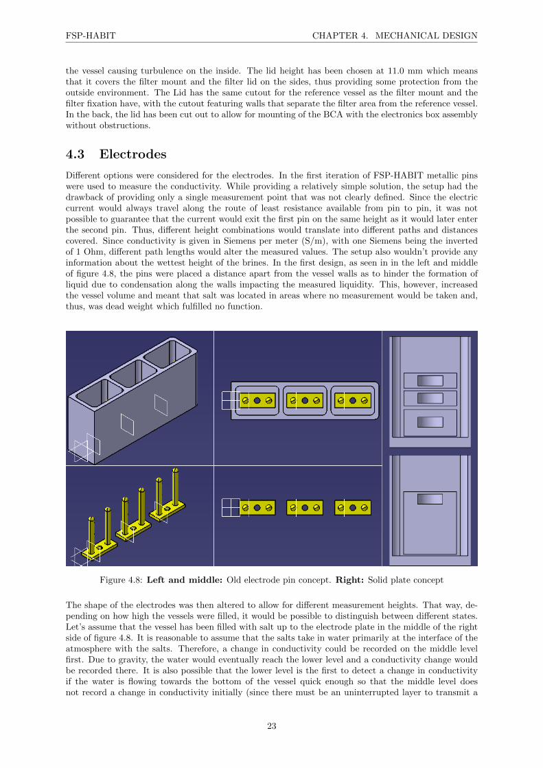
FSP-HABIT CHAPTER 4. MECHANICAL DESIGN
the vessel causing turbulence on the inside. The lid height has been chosen at 11.0 mm which meansthat it covers the filter mount and the filter lid on the sides, thus providing some protection from theoutside environment. The Lid has the same cutout for the reference vessel as the filter mount and thefilter fixation have, with the cutout featuring walls that separate the filter area from the reference vessel.In the back, the lid has been cut out to allow for mounting of the BCA with the electronics box assemblywithout obstructions.
4.3 Electrodes
Different options were considered for the electrodes. In the first iteration of FSP-HABIT metallic pinswere used to measure the conductivity. While providing a relatively simple solution, the setup had thedrawback of providing only a single measurement point that was not clearly defined. Since the electriccurrent would always travel along the route of least resistance available from pin to pin, it was notpossible to guarantee that the current would exit the first pin on the same height as it would later enterthe second pin. Thus, different height combinations would translate into different paths and distancescovered. Since conductivity is given in Siemens per meter (S/m), with one Siemens being the invertedof 1 Ohm, different path lengths would alter the measured values. The setup also wouldn’t provide anyinformation about the wettest height of the brines. In the first design, as seen in in the left and middleof figure 4.8, the pins were placed a distance apart from the vessel walls as to hinder the formation ofliquid due to condensation along the walls impacting the measured liquidity. This, however, increasedthe vessel volume and meant that salt was located in areas where no measurement would be taken and,thus, was dead weight which fulfilled no function.
Figure 4.8: Left and middle: Old electrode pin concept. Right: Solid plate concept
The shape of the electrodes was then altered to allow for different measurement heights. That way, de-pending on how high the vessels were filled, it would be possible to distinguish between different states.Let’s assume that the vessel has been filled with salt up to the electrode plate in the middle of the rightside of figure 4.8. It is reasonable to assume that the salts take in water primarily at the interface of theatmosphere with the salts. Therefore, a change in conductivity could be recorded on the middle levelfirst. Due to gravity, the water would eventually reach the lower level and a conductivity change wouldbe recorded there. It is also possible that the lower level is the first to detect a change in conductivityif the water is flowing towards the bottom of the vessel quick enough so that the middle level doesnot record a change in conductivity initially (since there must be an uninterrupted layer to transmit a
23
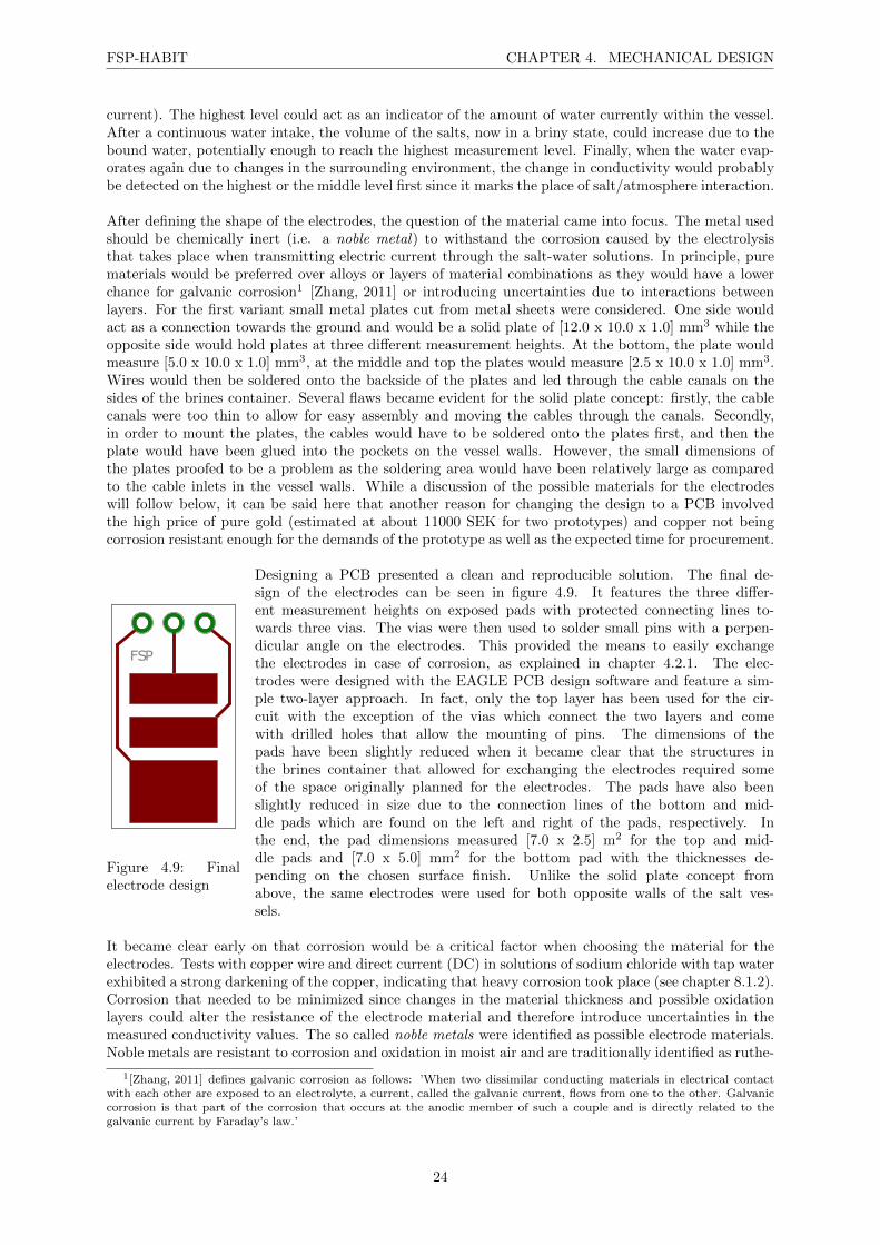
FSP-HABIT CHAPTER 4. MECHANICAL DESIGN
current). The highest level could act as an indicator of the amount of water currently within the vessel.After a continuous water intake, the volume of the salts, now in a briny state, could increase due to thebound water, potentially enough to reach the highest measurement level. Finally, when the water evap-orates again due to changes in the surrounding environment, the change in conductivity would probablybe detected on the highest or the middle level first since it marks the place of salt/atmosphere interaction.
After defining the shape of the electrodes, the question of the material came into focus. The metal usedshould be chemically inert (i.e. a noble metal) to withstand the corrosion caused by the electrolysisthat takes place when transmitting electric current through the salt-water solutions. In principle, purematerials would be preferred over alloys or layers of material combinations as they would have a lowerchance for galvanic corrosion1 [Zhang, 2011] or introducing uncertainties due to interactions betweenlayers. For the first variant small metal plates cut from metal sheets were considered. One side wouldact as a connection towards the ground and would be a solid plate of [12.0 x 10.0 x 1.0] mm3 while theopposite side would hold plates at three different measurement heights. At the bottom, the plate wouldmeasure [5.0 x 10.0 x 1.0] mm3, at the middle and top the plates would measure [2.5 x 10.0 x 1.0] mm3.Wires would then be soldered onto the backside of the plates and led through the cable canals on thesides of the brines container. Several flaws became evident for the solid plate concept: firstly, the cablecanals were too thin to allow for easy assembly and moving the cables through the canals. Secondly,in order to mount the plates, the cables would have to be soldered onto the plates first, and then theplate would have been glued into the pockets on the vessel walls. However, the small dimensions ofthe plates proofed to be a problem as the soldering area would have been relatively large as comparedto the cable inlets in the vessel walls. While a discussion of the possible materials for the electrodeswill follow below, it can be said here that another reason for changing the design to a PCB involvedthe high price of pure gold (estimated at about 11000 SEK for two prototypes) and copper not beingcorrosion resistant enough for the demands of the prototype as well as the expected time for procurement.
FSP
Figure 4.9: Finalelectrode design
Designing a PCB presented a clean and reproducible solution. The final de-sign of the electrodes can be seen in figure 4.9. It features the three differ-ent measurement heights on exposed pads with protected connecting lines to-wards three vias. The vias were then used to solder small pins with a perpen-dicular angle on the electrodes. This provided the means to easily exchangethe electrodes in case of corrosion, as explained in chapter 4.2.1. The elec-trodes were designed with the EAGLE PCB design software and feature a sim-ple two-layer approach. In fact, only the top layer has been used for the cir-cuit with the exception of the vias which connect the two layers and comewith drilled holes that allow the mounting of pins. The dimensions of thepads have been slightly reduced when it became clear that the structures inthe brines container that allowed for exchanging the electrodes required someof the space originally planned for the electrodes. The pads have also beenslightly reduced in size due to the connection lines of the bottom and mid-dle pads which are found on the left and right of the pads, respectively. Inthe end, the pad dimensions measured [7.0 x 2.5] m2 for the top and mid-dle pads and [7.0 x 5.0] mm2 for the bottom pad with the thicknesses de-pending on the chosen surface finish. Unlike the solid plate concept fromabove, the same electrodes were used for both opposite walls of the salt ves-sels.
It became clear early on that corrosion would be a critical factor when choosing the material for theelectrodes. Tests with copper wire and direct current (DC) in solutions of sodium chloride with tap waterexhibited a strong darkening of the copper, indicating that heavy corrosion took place (see chapter 8.1.2).Corrosion that needed to be minimized since changes in the material thickness and possible oxidationlayers could alter the resistance of the electrode material and therefore introduce uncertainties in themeasured conductivity values. The so called noble metals were identified as possible electrode materials.Noble metals are resistant to corrosion and oxidation in moist air and are traditionally identified as ruthe-
1[Zhang, 2011] defines galvanic corrosion as follows: ’When two dissimilar conducting materials in electrical contactwith each other are exposed to an electrolyte, a current, called the galvanic current, flows from one to the other. Galvaniccorrosion is that part of the corrosion that occurs at the anodic member of such a couple and is directly related to thegalvanic current by Faraday’s law.’
24
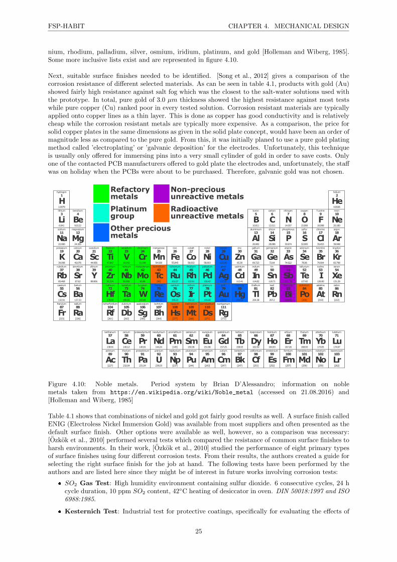
FSP-HABIT CHAPTER 4. MECHANICAL DESIGN
nium, rhodium, palladium, silver, osmium, iridium, platinum, and gold [Holleman and Wiberg, 1985].Some more inclusive lists exist and are represented in figure 4.10.
Next, suitable surface finishes needed to be identified. [Song et al., 2012] gives a comparison of thecorrosion resistance of different selected materials. As can be seen in table 4.1, products with gold (Au)showed fairly high resistance against salt fog which was the closest to the salt-water solutions used withthe prototype. In total, pure gold of 3.0 µm thickness showed the highest resistance against most testswhile pure copper (Cu) ranked poor in every tested solution. Corrosion resistant materials are typicallyapplied onto copper lines as a thin layer. This is done as copper has good conductivity and is relativelycheap while the corrosion resistant metals are typically more expensive. As a comparison, the price forsolid copper plates in the same dimensions as given in the solid plate concept, would have been an order ofmagnitude less as compared to the pure gold. From this, it was initially planed to use a pure gold platingmethod called ’electroplating’ or ’galvanic deposition’ for the electrodes. Unfortunately, this techniqueis usually only offered for immersing pins into a very small cylinder of gold in order to save costs. Onlyone of the contacted PCB manufacturers offered to gold plate the electrodes and, unfortunately, the staffwas on holiday when the PCBs were about to be purchased. Therefore, galvanic gold was not chosen.
nitrogen
14.007
N7
helium
He4.0026
2
neon
Ne20.180
10f uorine
F18.998
9oxygen
O15.999
8carbon
C12.011
6boron
B10.811
5
argon
Ar39.948
18chlorine
Cl35.453
17sulfur
S32.065
16phosphorus
P30.974
15silicon
Si28.086
14aluminium
Al26.982
13
krypton
Kr83.798
36bromine
Br79.904
35selenium
Se78.96
34arsenic
As74.922
33germanium
Ge72.64
32gallium
Ga69.723
31zinc
Zn65.38
30copper
Cu63.546
29nickel
Ni58.693
28cobalt
Co58.933
27iron
Fe55.845
26manganese
Mn54.938
25chromium
Cr51.996
24vanadium
V50.942
23titanium
Ti47.867
22scandium
Sc44.956
21calcium
Ca40.078
20potassium
K39.098
19
magnesium
Mg24.305
12sodium
Na22.990
11
beryllium
Be9.0122
4lithium
Li6.941
3
hydrogen
H1.0079
1
xenon
Xe131.29
54iodine
I126.90
53tellurium
Te127.60
52antimony
Sb121.76
51tin
Sn118.71
50indium
In114.82
49cadmium
Cd112.41
48silver
Ag107.87
47palladium
Pd106.42
46rhodium
Rh102.91
45ruthenium
Ru101.07
44technetium
Tc[98]
43molybdenum
Mo95.96
42niobium
Nb92.906
41zirconium
Zr91.224
40yttrium
Y88.906
39strontium
Sr87.62
38rubidium
Rb85.468
37
radon
Rn[222]
86astatine
At[210]
85polonium
Po[209]
84bismuth
Bi208.98
83lead
Pb207.2
82
dysprosium
Dy162.50
66terbium
Tb158.93
65gadolinium
Gd157.25
64europium
Eu151.96
63samarium
Sm150.36
62promethium
Pm[145]
61neodymium
Nd144.24
60praseodymium
Pr140.91
59cerium
Ce140.12
58lanthanum
La138.91
57
barium
Ba137.33
56caesium
Cs132.91
55
roentgenium
Rg[272]
111darmstadtium
Ds[271]
110meitnerium
Mt[268]
109hassium
Hs[277]
108bohrium
Bh[264]
107seaborgium
Sg[266]
106dubnium
Db[262]
105rutherfordium
Rf[261]
104radium
Ra[226]
88francium
Fr[223]
87
lutetium
Lu174.97
71ytterbium
Yb173.05
70thulium
Tm168.93
69erbium
Er167.26
68holmium
Ho164.93
67
thallium
Tl204.38
81mercury
Hg200.59
80gold
Au196.97
79platinum
Pt195.08
78iridium
Ir192.22
77osmium
Os190.23
76rhenium
Re186.21
75tungsten
W183.84
74tantalum
Ta180.95
73hafnium
Hf178.49
72
berkelium
Bk[247]
97lawrencium
Lr[262]
103nobelium
No[259]
102mendelevium
Md[258]
101fermium
Fm[257]
100einsteinium
Es[252]
99californium
Cf[251]
98curium
Cm[247]
96americium
Am[243]
95plutonium
Pu[244]
94neptunium
Np[237]
93uranium
U238.03
92protactinium
Pa231.04
91thorium
Th232.04
90actinium
Ac[227]
89
Refactorymetals
Platinumgroup
Other preciousmetals
Non-preciousunreactive metals
Radioactiveunreactive metals
Figure 4.10: Noble metals. Period system by Brian D’Alessandro; information on noblemetals taken from https://en.wikipedia.org/wiki/Noble_metal (accessed on 21.08.2016) and[Holleman and Wiberg, 1985]
Table 4.1 shows that combinations of nickel and gold got fairly good results as well. A surface finish calledENIG (Electroless Nickel Immersion Gold) was available from most suppliers and often presented as thedefault surface finish. Other options were available as well, however, so a comparison was necessary:[Ozkok et al., 2010] performed several tests which compared the resistance of common surface finishes toharsh environments. In their work, [Ozkok et al., 2010] studied the performance of eight primary typesof surface finishes using four different corrosion tests. From their results, the authors created a guide forselecting the right surface finish for the job at hand. The following tests have been performed by theauthors and are listed here since they might be of interest in future works involving corrosion tests:
SO2 Gas Test: High humidity environment containing sulfur dioxide. 6 consecutive cycles, 24 hcycle duration, 10 ppm SO2 content, 42C heating of desiccator in oven. DIN 50018:1997 and ISO6988:1985.
Kesternich Test: Industrial test for protective coatings, specifically for evaluating the effects of
25

FSP-HABIT CHAPTER 4. MECHANICAL DESIGN
Material H2S SO2 Cl2/4 d NO2 NH3 air/120C Salt fogAu, 3 µm 1 1 2 1 1 1 1AuCo1, 3 µm 1 1 3 1 1 3 1AuNi10, 3 µm 2 2 1 1 1 2 1Au, 0.2 µm 1 3 3 3 1 3 2Ni, 3 µm/Au, 1 µm 3 1 3 1 1 1 1Ni, 3 µm/Au, 3 µm 1 1 3 1 1 1 1Ag, 10 µm 2 1 2 3 1 1 2Ni/Pd, 3 µm 2 2 3 1 1 1 1Chem. Sn, 0.5 µm 2 2 3 3 1 3 2electroplated Sn, dull, 15 µm 1 3 1 1 1 1 2electroplated Sn, bright, 15 µm 1 2 3 1 1 1 2PbSn 40/60, 6 µm 1 1 2 1 1 1 2hot dip tin, 6 µm 1 1 3 1 1 1 2Ni, 3 µm 3 3 3 2 2 2 2Cu 3 3 3 3 3 3 3
Table 4.1: Corrosion resistance of selected metals: 1 = high; 2 = fair; 3 = poor. From [Song et al., 2012]
acid rain. 6 consecutive cycles, 24 h cycle duration, 8 h of heating at 40C and 100% RH, followedby 16 h of ventilation at <75% RH, 200 ml SO2 content in a 300 l chamber. DIN EN ISO 6988.
Salt Spray Test: Accelerated corrosion tests, simulating a corrosive attack in a harsh marineclimate. Test solution: 50 g/l NaCl, pH = 6.0-7.5, 35C, 1.5 ml/h spray volume (16 h average).DIN 50021/ISO 9227.
Surface Insulation Resistance Test (SIR): Assess the potential failure of PCB assembliesthrough corrosion and/or ionic contamination by measuring the electrical resistance between twoconductors. Checks for connections/short circuits caused by electrolytes. 7 days of testing at 85C,85% RH, 50 V bias.
The tested surface finishes can be seen in table 4.2.
Surface Finish ThicknessENIG (7-9.5 w% P) Med P Ni 5 µm / Au 0.07 µmENIG (10-13 w% P) High P Ni 5 µm / Au 0.07 µmENEPIG (Ni-P / Pd / Au) Ni 5 µm / Pd 0.1 µm / Au 0.03 µmENEPIG (Ni-P / Pd-P / Au) Ni 5 µm / Pd-P 0.1 µm / Au 0.03 µmImmersion Sn Sn 0.8-0.9 µmImmersion Ag Ag 0.3-0.5 µmOSP Organic Surface
Table 4.2: Summary of surface finish specifications. From [Ozkok et al., 2010]
Figure 4.11 shows the corrosion resistance of all tested surface finishes on average, i.e. as combinedresults of the tests described before. The clear winner appears to be immersion tin. Immersion tin wasno viable choice for the electrodes, however. This is due to the special nature of the conductivity sensor:since the conductivity sensor is using alternating current (AC) for its measurements, the phenomenonthat causes the immersion tin to be so corrosion resistant in most cases does not work for FSP-HABITsmeasurements. The effect, known as passivity, is defined as follows: ’A condition in which a piece ofmetal, because of an impervious covering of oxide or other compound, has a potential that is much morepositive than that of the metal in the active state.’ [Roberge, 2000]. Simply put, this means that an oxidelayer protects the metal underneath it from further corrosion. As can be taken from the definition, themetal retains its corrosion protection due to the higher potential it has compared to the surrounding me-dia. However, [Brenna et al., 2011] remarks that AC causes the local breakdown of the nanosized passivelayer. It is likely that the oscillations cause the corrosion, probably due to the different time constantsassociated with metal2 dissolution (fast) and the formation of the passive layer (slower) [Nielsen, 2005].
2[Nielsen, 2005] performed their research on iron
26

FSP-HABIT CHAPTER 4. MECHANICAL DESIGN
In effect, immersion tin was not suitable for the protection of the electrodes since a passive layer wasundesirable as it could affect the measurement.
The next best choice found in figure 4.11 is ENIG (Electroless Nickel Immersion Gold) with a highphosphor content (as described in table 4.2). This would have been the preferred choice for the electrodes.When contacting manufacturers, however, the nickel content was usually found in the medium regime (7-9.5 wt%). Since the electrode procurement was done fairly late in the creation of the FSP-HABIT, highphosphor ENIG was not a viable choice. In the end, the next best choice, ENEPIG (Electroless NickelElectroless Palladium Immersion Gold), was chosen. The difference between ENIG and ENEPIG is alayer of the noble metal palladium between the nickel and the gold layer. Also, since it was comparativelycheap, medium phosphor ENIG was ordered to have a base for comparison. The ENEPIG electrodeswere ordered from LeitOn GmbH and the ENIG electrodes from Wurth Elektronik.
OSPDeficient 0
1
Poor 2
3
Adequate 4
5
Satisfactory 6
7
Good 8
9
Excellent 10
ENIGMedium
Phosphor
ENIGHigh
Phosphor
ENEPIGPure Pd
ENEPIGPd-
Phosphor
ImmersionSilver
ImmersionTin
Figure 4.11: Summary of corrosion test results for tested finishes. From [Ozkok et al., 2010]
Figure 4.12: Thefinalized electrodes.Here with ENIG sur-face finish.
Since the electrodes were relatively small for printed circuit boards, several elec-trodes were created on each PCB and then pre-milled for easy break out. Whenthe electrodes arrived at campus, the individual electrodes were broken out fromthe PCB and then the predetermined breaking points were rasped smooth. Theelectrodes were then cleaned with water and dried with tissues and pressuredair. To prepare the electrodes for easy mounting, small pins were then solderedonto the electrodes. Before using the electrodes with FSP-HABIT, the resistancefrom each measurement plate to the end of the corresponding connection pin wasmeasured. The resistance between the points was measured as well to ensurethat their resistance was indicated as open loop by the multimeter. The finishedelectrodes can be seen in figure 4.12.
27
FSP-HABIT CHAPTER 4. MECHANICAL DESIGN
4.4 Electronics Box Assembly (EBox) Overview
The Electronics Box assembly (EBox) fulfills several functions: 1) Hold the electronics of the AC con-ductivity meter, mounted on an Euro-Card. 2) hold the electronics of six environmental sensors (relativehumidity, pressure, ground temperature, 3 x air temperature). 3) Hold the controlling ARDUINO. 4)Hold the battery and 5) the SD-Card reader. 6) Protect all of the above from the outside environmentwhile providing access to it for the environmental sensors. Figure 4.13 shows the electronics box assemblyof FSP-HABIT. From top to bottom: Lids, ARDUINO and Battery/SD housing, the main electronicscompartment (EBox Main), four legs.
Legs (4x)
EBox Main:Electronics, RH and GTS
EBox Lid:ARDUINO and Battery/SD housing
ARDUINO and Battery/SD Lids
Figure 4.13: The Electronics Box assembly (EBox) overview
28
FSP-HABIT CHAPTER 4. MECHANICAL DESIGN
Lids: The lids have the function of keeping the ARDUINO, the batteries and the SD-Card reader, aswell as the DC-DC power converter save from the surrounding weather (e.g. rain, strong winds). Theyare mounted to the EBox Lid using two screws each.
Ebox Lid: The EBox Lid is placed on top of the EBox Main and connected using six screws. Itholds the ARDUINO, the batteries and the SD-Card reader, as well as the DC-DC power converter.Cutouts are used to move cables from the EBox Lid to the EBox Main. The EBox Lid also featuresa compartment for the pressure sensor. Two mounting spots are found in the front that are used toconnect the EBox Lid, Main, and the BCA using two screws.
EBox Main: The EBox holds the main circuit board and the relative humidity and ground temperaturesensors. It features six mounting spots for the EBox Lid, two mountings spots for the BCA and fourmounting spots for the legs. It also has a cutout to lead the cables from the BCA to the electronics board.
Legs: Used to thermally decouple the prototype from the ground and heighten the prototype overwet surfaces.
4.5 Electronics Box Assembly (EBox) Detail
4.5.1 EBox Main
Top
Right
25
Left
Front Rear
Bottom
106
177.5
GTS
CableInlet
RHS
CircuitBoard
Figure 4.14: EBox Main detail
Design driver: Hold circuit board and protect it from environment.
The EBox Main holds the circuit board for the AC conductivity meter and the environmental sensors.The largest part of it is a rectangular, empty, area with 4 mounting spots on the edges. This area holdsthe [160 x 100] mm2 circuit board while the mounting spots raise the board 4.5 mm above the bottom ofthe EBox Main floor. That way, soldering spots and sticking out cable ends have enough room while atthe same time being slightly better protected should a liquid film form on the bottom due to condensa-tion or high humidity in the surrounding air. In the front wall, a cutout allows cables from the BCA tobe led to the circuit board. The surrounding rectangular structure seen in figure 4.14 has a curvature onits bottom that helps in pushing the cables through the narrow slid and up to the main chamber. Twosections of its wall towards the circuit board are also heightened so that they restrict the movement ofthe circuit board during mounting.
29
FSP-HABIT CHAPTER 4. MECHANICAL DESIGN
On the right side, a structure for the Relative Humidity Sensor (RHS) (chapter 5.3.2) has been created.The RHS has been raised 16.15 mm so that is found 5.35 mm below the EBox Lid which protects theRHS from rain fall. The RHS is then laid into the cut out area and held in place by a small rectangularpiece of plastic that is inserted into the slid from the top. The piece is then glued in place so that theRHS won’t be able to move. Towards the outside walls, the RHS is within a compartment with severalcutouts on the bottom, and on two perpendicular walls. The cutouts have been designed with smoothedges as not to hinder air flowing through the compartment. The EBox Lid on top also presents someprotection from heating up of the RHS through Sun light.
The Ground Temperature Sensor (GTS) (chapter 5.3.1) is found opposite of the RHS. Its mount has around shape with a slid on top into which the GTS can be pressed. The GTS is mounted at a 30 anglewhich allows it to fully utilize its 90 field of view. The sensor is protected from rain fall and heatingthrough direct Sun light by a round shield. The shield sticks out 4.0 mm from the outside wall, providingshadow to the GTS while avoiding obstruction of its field of view.
The EBox Main also features reinforced mounting spots for four legs. The cable inlet, RHS mount, andthe GTS mount can be seen in detail in figure 4.15.
Figure 4.15: EBox details. Far left: Cable inlet; Left and middle: RHS mount; Right and farright: GTS mount.
4.5.2 EBox Lid
Design driver: Compartments for the ARDUINO, the batteries, and the SD-card reader.
The EBox Lid is mounted on top of the EBox Main to which it is secured by using six screws. In the frontit has two mounting spots that are connected with the BCA and the EBox Main. The mounting spotsare reinforced by two struts so that they can hold part of the shearing force that is caused by the BCAacting like a lever onto the EBox Lid. The ARDUINO is mounted in the middle compartment. Fourprotrusions are used to raise the ARDUINO 4.0 mm above the ground. This allows for several cables tobe led through underneath the board. A cutout of [45.0 x 12.0] mm2 in front of the ARDUINO is used tomove the major part of the cables from the electronics board in the EBox Main to the ARDUINO. Twomounting spots with a 2.25 mm radius are found in the front which are used by the lid’s bolts and help insecuring the lid on top of the ARDUINO compartment. Two through-holes for screws are then used tofixate the lid to the compartment. Opposite of the cable cutout, a small cutout of [10.0 x 5.0] mm2 is usedto transfer power from the battery compartment to the ARDUINO. The last compartment is comprisedof two parts, one holding an eight AA battery holder of type BH48AASF while the second holds a smallcircuit board with an Adafruit Micro SD breakout board, a Traco DC/DC step-down converter of typeTSR 1-2450, and connecting cables for a BMP180 pressure sensor breakout board. The small circuitboard, like the ARDUINO, is raised by 4.0 mm protrusions which keep the area under the board free forcables. A cutout of [14.0 x 10.0] mm2 is used to connect the small circuit board with the main circuitboard, located in the EBox Main. Like the ARDUINO compartment, the battery/SD compartment hasthree mounting spots with a 2.25 mm radius for the lid’s bolts which help in securing the lid on topof the battery/SD compartment. Again, two through-holes for screws are then used to fixate the lidto the compartment. It also features a small wall in the middle of the compartment which helps tokeep the battery holder in place. Finally, a small compartment of [25.0 x 4.5 x 32.0] mm3 has beendesigned to hold the BMP180 pressure sensor breakout board. The breakout board is mounted verticallyin the compartment, held in position by the walls and by its soldered pins which have been glued to the
30
FSP-HABIT CHAPTER 4. MECHANICAL DESIGN
Top
Front
Right34
Left
Bottom
177.5
114
Rear
ARDUINO
Batteries
SD-Card ReaderDC-DC Converter
PS
Figure 4.16: EBox Lid detail
prototype. A cutout of [4.0 x 4.0] mm2 has been placed 9.5 mm below the lid which corresponds to theheight of the air hole of the pressure sensor. Another cutout of [24.5 x 3.0]mm2, in combination withthe first one, allows for air to exchange freely and prevents situations where wind flowing around theoutside walls creates differences between the inside and the environment pressure. Two further strutsinside the compartment help to keep the breakout board in place. The bottom is at an angle to preventthe gathering of water.
4.5.3 ARDUINO And Battery Lids; Legs
Design driver: Closure for compartments, raise level of prototype.
The design of the lids is straight forward: they cover the corresponding compartments and are fixatedwith two screws each. Two bolts in the case of the ARDUINO lid and three bolts in the case of thebattery/SD lid help in keeping the lids in place. Their radius is 2.0 mm and they are 10.0 mm high. Thelids overlap the compartments by 1.2 mm to offer protection from spray water. The legs have a 5.0 mmradius with a through-hole with a 2.25 mm radius. The legs are hollow inside, allowing for a screw tobe inserted from below and then hidden inside. For that, the lower part’s inside radius of the leg is 4.0mm, stretching up 15.0 mm of the total 20.0 mm height of the legs.
31
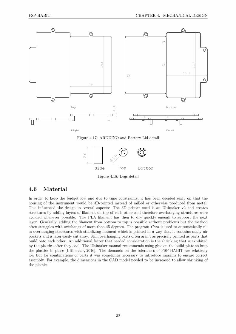
FSP-HABIT CHAPTER 4. MECHANICAL DESIGN
Top
75
103
Bottom
117
73.5
Right
2.8
Front
Figure 4.17: ARDUINO and Battery Lid detail
Side
20
Top
10
Bottom
Figure 4.18: Legs detail
4.6 Material
In order to keep the budget low and due to time constraints, it has been decided early on that thehousing of the instrument would be 3D-printed instead of milled or otherwise produced from metal.This influenced the design in several aspects: The 3D printer used is an Ultimaker v2 and createsstructures by adding layers of filament on top of each other and therefore overhanging structures wereavoided whenever possible. The PLA filament has then to dry quickly enough to support the nextlayer. Generally, adding the filament from bottom to top is possible without problems but the methodoften struggles with overhangs of more than 45 degrees. The program Cura is used to automatically fillin overhanging structures with stabilizing filament which is printed in a way that it contains many airpockets and is later easily cut away. Still, overhanging parts often aren’t as precisely printed as parts thatbuild onto each other. An additional factor that needed consideration is the shrinking that is exhibitedby the plastics after they cool. The Ultimaker manual recommends using glue on the build-plate to keepthe plastics in place [Ultimaker, 2016]. The demands on the tolerances of FSP-HABIT are relativelylow but for combinations of parts it was sometimes necessary to introduce margins to ensure correctassembly. For example, the dimensions in the CAD model needed to be increased to allow shrinking ofthe plastic.
32

Chapter 5
Electrical Design
5.1 ARDUINO
The starting point of the FSP-HABIT electrical design was its micro-controller. To save on developmenttime, it was decided to use an ARDUINO board. This would avoid the need to choose and connectcommercial microprocessors and provided a functional base for development. ARDUINOs are open-source electronic prototyping platforms that are widely used by hobbyists and universities. It comeswith its own programming language based on Wiring and a development suite, the ARDUINO Software(IDE). Low prices and accessibility, combined with the open source approach are likely reasons for thewidespread use of ARDUINOs around the globe. Several options exist when choosing an ARDUINO.The usual entry point is the ARDUINO Uno, currently available in the third revision, which is fairlyaffordable at just under 30 Euros. It is powered by a ATmega328 micro-controller and has 14 digitalinputs/outputs of which six can be used for pulse width modulation (PWM), as well as six analoginputs. Since the prototype was going to have six vessels with three measurement heights each, meaningthat there were 18 points that needed to be controlled somehow, other options with more I/Os wereconsidered next. The ARDUINO Mega 2560 Rev. 3 is essentially an upgraded ARDUINO Uno: it hasan ATmega2560 micro-controller, 54 digital I/Os, of which 15 can be used for PWM, and 16 analoginputs. Another option would have been the ARDUINO Due which has been retired from ARDUINOsproduct line by the time of the writing of this report. The board is similarly sized as the Mega with 54digital I/Os (12 for PWM) and twelve analog inputs. Main differences to the Mega boards are the severaltimes higher clock speed and its operating voltage. Unlike most Arduino boards, the Arduino Due boardruns at 3.3 V. The higher clock speed was deemed unnecessary which left the different operating voltageas a major difference between the boards. Since at the time of the choosing of the board it was still notknown which sensors would be purchased and how exactly the conductivity sensor would be designed,it was decided to go with the 5 V option of the Mega. Another influencing factor was the fact that forthe standard ARDUINOs, running with 5 V, a large amount of tutorials and knowledge is available. Anoverview of the different options that have been considered can be seen in table 5.1.
33
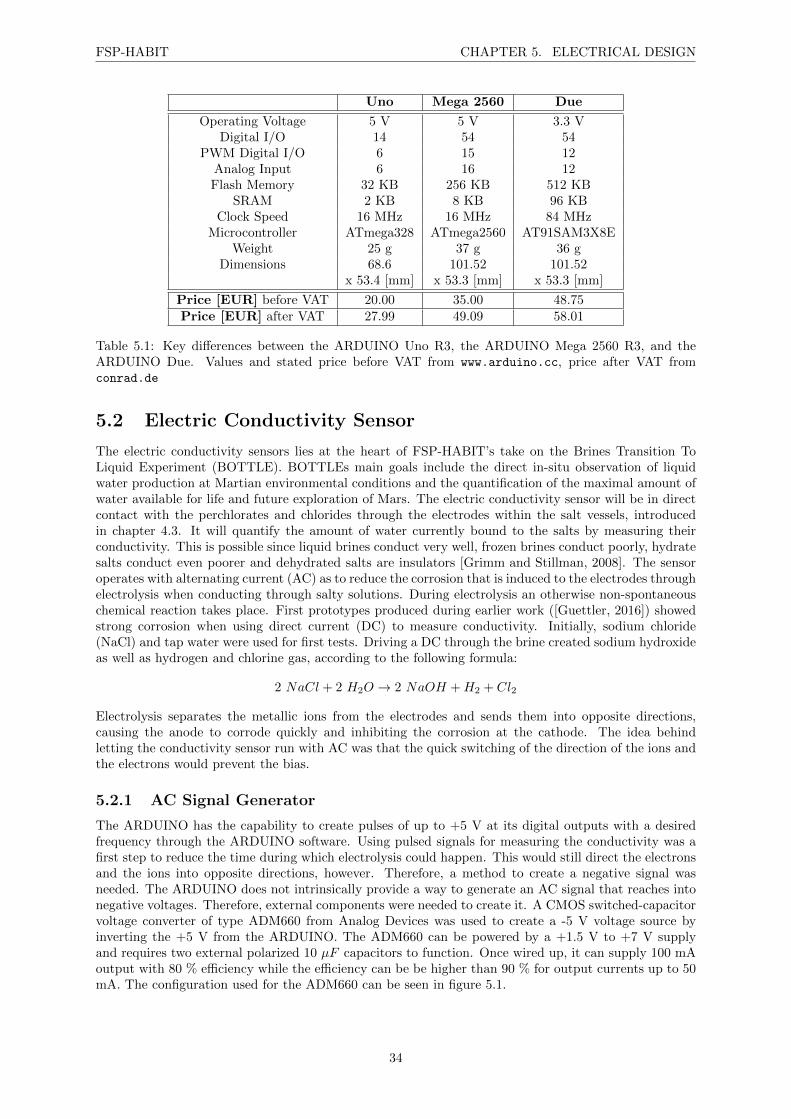
FSP-HABIT CHAPTER 5. ELECTRICAL DESIGN
Uno Mega 2560 Due
Operating Voltage 5 V 5 V 3.3 VDigital I/O 14 54 54
PWM Digital I/O 6 15 12Analog Input 6 16 12Flash Memory 32 KB 256 KB 512 KB
SRAM 2 KB 8 KB 96 KBClock Speed 16 MHz 16 MHz 84 MHz
Microcontroller ATmega328 ATmega2560 AT91SAM3X8EWeight 25 g 37 g 36 g
Dimensions 68.6 101.52 101.52x 53.4 [mm] x 53.3 [mm] x 53.3 [mm]
Price [EUR] before VAT 20.00 35.00 48.75Price [EUR] after VAT 27.99 49.09 58.01
Table 5.1: Key differences between the ARDUINO Uno R3, the ARDUINO Mega 2560 R3, and theARDUINO Due. Values and stated price before VAT from www.arduino.cc, price after VAT fromconrad.de
5.2 Electric Conductivity Sensor
The electric conductivity sensors lies at the heart of FSP-HABIT’s take on the Brines Transition ToLiquid Experiment (BOTTLE). BOTTLEs main goals include the direct in-situ observation of liquidwater production at Martian environmental conditions and the quantification of the maximal amount ofwater available for life and future exploration of Mars. The electric conductivity sensor will be in directcontact with the perchlorates and chlorides through the electrodes within the salt vessels, introducedin chapter 4.3. It will quantify the amount of water currently bound to the salts by measuring theirconductivity. This is possible since liquid brines conduct very well, frozen brines conduct poorly, hydratesalts conduct even poorer and dehydrated salts are insulators [Grimm and Stillman, 2008]. The sensoroperates with alternating current (AC) as to reduce the corrosion that is induced to the electrodes throughelectrolysis when conducting through salty solutions. During electrolysis an otherwise non-spontaneouschemical reaction takes place. First prototypes produced during earlier work ([Guettler, 2016]) showedstrong corrosion when using direct current (DC) to measure conductivity. Initially, sodium chloride(NaCl) and tap water were used for first tests. Driving a DC through the brine created sodium hydroxideas well as hydrogen and chlorine gas, according to the following formula:
2 NaCl + 2 H2O → 2 NaOH +H2 + Cl2
Electrolysis separates the metallic ions from the electrodes and sends them into opposite directions,causing the anode to corrode quickly and inhibiting the corrosion at the cathode. The idea behindletting the conductivity sensor run with AC was that the quick switching of the direction of the ions andthe electrons would prevent the bias.
5.2.1 AC Signal Generator
The ARDUINO has the capability to create pulses of up to +5 V at its digital outputs with a desiredfrequency through the ARDUINO software. Using pulsed signals for measuring the conductivity was afirst step to reduce the time during which electrolysis could happen. This would still direct the electronsand the ions into opposite directions, however. Therefore, a method to create a negative signal wasneeded. The ARDUINO does not intrinsically provide a way to generate an AC signal that reaches intonegative voltages. Therefore, external components were needed to create it. A CMOS switched-capacitorvoltage converter of type ADM660 from Analog Devices was used to create a -5 V voltage source byinverting the +5 V from the ARDUINO. The ADM660 can be powered by a +1.5 V to +7 V supplyand requires two external polarized 10 µF capacitors to function. Once wired up, it can supply 100 mAoutput with 80 % efficiency while the efficiency can be be higher than 90 % for output currents up to 50mA. The configuration used for the ADM660 can be seen in figure 5.1.
34
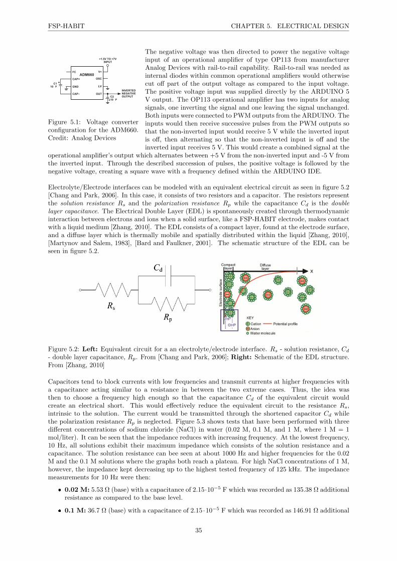
FSP-HABIT CHAPTER 5. ELECTRICAL DESIGN
+
+
+1.5V TO +7VINPUT
C110 F
C210 F
INVERTEDNEGATIVEOUTPUT
ADM660FC
CAP+
GND
CAP–
V+
OSC
LV
OUT
Figure 5.1: Voltage converterconfiguration for the ADM660.Credit: Analog Devices
The negative voltage was then directed to power the negative voltageinput of an operational amplifier of type OP113 from manufacturerAnalog Devices with rail-to-rail capability. Rail-to-rail was needed asinternal diodes within common operational amplifiers would otherwisecut off part of the output voltage as compared to the input voltage.The positive voltage input was supplied directly by the ARDUINO 5V output. The OP113 operational amplifier has two inputs for analogsignals, one inverting the signal and one leaving the signal unchanged.Both inputs were connected to PWM outputs from the ARDUINO. Theinputs would then receive successive pulses from the PWM outputs sothat the non-inverted input would receive 5 V while the inverted inputis off, then alternating so that the non-inverted input is off and theinverted input receives 5 V. This would create a combined signal at the
operational amplifier’s output which alternates between +5 V from the non-inverted input and -5 V fromthe inverted input. Through the described succession of pulses, the positive voltage is followed by thenegative voltage, creating a square wave with a frequency defined within the ARDUINO IDE.
Electrolyte/Electrode interfaces can be modeled with an equivalent electrical circuit as seen in figure 5.2[Chang and Park, 2006]. In this case, it consists of two resistors and a capacitor. The resistors representthe solution resistance Rs and the polarization resistance Rp while the capacitance Cd is the doublelayer capacitance. The Electrical Double Layer (EDL) is spontaneously created through thermodynamicinteraction between electrons and ions when a solid surface, like a FSP-HABIT electrode, makes contactwith a liquid medium [Zhang, 2010]. The EDL consists of a compact layer, found at the electrode surface,and a diffuse layer which is thermally mobile and spatially distributed within the liquid [Zhang, 2010],[Martynov and Salem, 1983], [Bard and Faulkner, 2001]. The schematic structure of the EDL can beseen in figure 5.2.
Figure 5.2: Left: Equivalent circuit for a an electrolyte/electrode interface. Rs - solution resistance, Cd
- double layer capacitance, Rp. From [Chang and Park, 2006]; Right: Schematic of the EDL structure.From [Zhang, 2010]
Capacitors tend to block currents with low frequencies and transmit currents at higher frequencies witha capacitance acting similar to a resistance in between the two extreme cases. Thus, the idea wasthen to choose a frequency high enough so that the capacitance Cd of the equivalent circuit wouldcreate an electrical short. This would effectively reduce the equivalent circuit to the resistance Rs,intrinsic to the solution. The current would be transmitted through the shortened capacitor Cd whilethe polarization resistance Rp is neglected. Figure 5.3 shows tests that have been performed with threedifferent concentrations of sodium chloride (NaCl) in water (0.02 M, 0.1 M, and 1 M, where 1 M = 1mol/liter). It can be seen that the impedance reduces with increasing frequency. At the lowest frequency,10 Hz, all solutions exhibit their maximum impedance which consists of the solution resistance and acapacitance. The solution resistance can bee seen at about 1000 Hz and higher frequencies for the 0.02M and the 0.1 M solutions where the graphs both reach a plateau. For high NaCl concentrations of 1 M,however, the impedance kept decreasing up to the highest tested frequency of 125 kHz. The impedancemeasurements for 10 Hz were then:
0.02 M: 5.53 Ω (base) with a capacitance of 2.15·10−5 F which was recorded as 135.38 Ω additionalresistance as compared to the base level.
0.1 M: 36.7 Ω (base) with a capacitance of 2.15 ·10−5 F which was recorded as 146.91 Ω additional
35
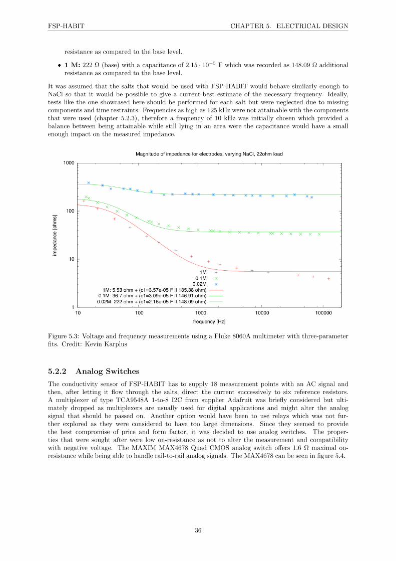
FSP-HABIT CHAPTER 5. ELECTRICAL DESIGN
resistance as compared to the base level.
1 M: 222 Ω (base) with a capacitance of 2.15 · 10−5 F which was recorded as 148.09 Ω additionalresistance as compared to the base level.
It was assumed that the salts that would be used with FSP-HABIT would behave similarly enough toNaCl so that it would be possible to give a current-best estimate of the necessary frequency. Ideally,tests like the one showcased here should be performed for each salt but were neglected due to missingcomponents and time restraints. Frequencies as high as 125 kHz were not attainable with the componentsthat were used (chapter 5.2.3), therefore a frequency of 10 kHz was initially chosen which provided abalance between being attainable while still lying in an area were the capacitance would have a smallenough impact on the measured impedance.
Figure 5.3: Voltage and frequency measurements using a Fluke 8060A multimeter with three-parameterfits. Credit: Kevin Karplus
5.2.2 Analog Switches
The conductivity sensor of FSP-HABIT has to supply 18 measurement points with an AC signal andthen, after letting it flow through the salts, direct the current successively to six reference resistors.A multiplexer of type TCA9548A 1-to-8 I2C from supplier Adafruit was briefly considered but ulti-mately dropped as multiplexers are usually used for digital applications and might alter the analogsignal that should be passed on. Another option would have been to use relays which was not fur-ther explored as they were considered to have too large dimensions. Since they seemed to providethe best compromise of price and form factor, it was decided to use analog switches. The proper-ties that were sought after were low on-resistance as not to alter the measurement and compatibilitywith negative voltage. The MAXIM MAX4678 Quad CMOS analog switch offers 1.6 Ω maximal on-resistance while being able to handle rail-to-rail analog signals. The MAX4678 can be seen in figure 5.4.
36
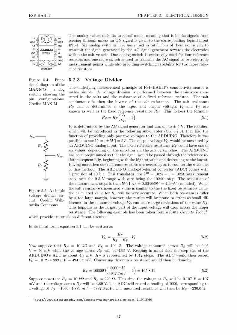
FSP-HABIT CHAPTER 5. ELECTRICAL DESIGN
16
15
14
13
12
11
10
9
1
2
3
4
5
6
7
8
IN2
COM2
NO2
V+V-
NO1
COM1
IN1
MAX4678 VL
NO3
COM3
IN3IN4
COM4
NO4
GND
DIP/TSSOP
Figure 5.4: Func-tional diagram of theMAX4678 analogswitch, showing thepin configurations.Credit: MAXIM
The analog switch defaults to an off mode, meaning that it blocks signals frompassing through unless an ON signal is given to the corresponding logical inputIN1-4. Six analog switches have been used in total, four of them exclusively totransmit the signal generated by the AC signal generator towards the electrodeswithin the salt vessels. One analog switch is exclusively used for four referenceresistors and one more switch is used to transmit the AC signal to two electrodemeasurement points while also providing switching capability for two more refer-ence resistors.
5.2.3 Voltage Divider
The underlying measurement principle of FSP-HABIT’s conductivity sensor israther simple: A voltage division is performed between the resistance mea-sured in the salts and the resistance of a fixed reference resistor. The saltconductance is then the inverse of the salt resistance. The salt resistanceRS can be determined if the input and output voltages VI and VO areknown as well as the fixed reference resistance RF . This follows the formula:
RS = RF
( VIVO− 1
)(5.1)
Figure 5.5: A simplevoltage divider cir-cuit. Credit: Wiki-media Commons
VI is determined by the AC signal generator and was set to ± 5 V. The rectifier,which will be introduced in the following sub-chapter (Ch. 5.2.5), then had thefunction of providing only positive voltages to the ARDUINO. Therefore it waspossible to use VI = | ± 5V | = 5V . The output voltage VO would be measured byan ARDUINO analog input. The fixed reference resistance RF could have one ofsix values, depending on the selection via the analog switches. The ARDUINOhas been programmed so that the signal would be passed through the reference re-sistors sequentially, beginning with the highest value and decreasing to the lowest.Having more then one reference resistors was necessary as to counter the weaknessof this method: The ARDUINO analog-to-digital converter (ADC) comes witha precision of 10 bit. This translates into 210 = 1024 − 1 = 1023 measurementsteps over the 0-5 V range with zero being the 1024th step. The resolution ofthe measurement steps is then 5V/1023 = 0.004889V = 4.9mV (rounded). Whenthe salt resistance’s measured value is similar to the the fixed resistance’s value,the calculated value for RS will be very accurate. When both resistances differby a too large margin, however, the results will be prone to errors as small dif-ferences in the measured voltage VO can cause large deviations of the value RS .This happens as the largest part of the input voltage will drop across the largerresistance. The following example has been taken from website Circuits Today1,
which provides tutorials on different circuits:
In its inital form, equation 5.1 can be written as
VO =RF
RS +RF· VI (5.2)
Now suppose that RF = 10 kΩ and RS = 100 Ω. The voltage measured across RS will be 0.05V = 50 mV while the voltage across RF will be 4.95 V. Keeping in mind that the step size of theARDUINO’s ADC is about 4.9 mV, RF is represented by 1012 steps. The ADC would then recordVO = 1012 · 4.889 mV = 4947.7 mV . Converting this into a resistance would then be done by:
RS = 10000Ω( 5000mV
4947.7mV− 1
)= 105.8 Ω (5.3)
Suppose now that RF = 10 kΩ and RS = 220 Ω. This time the voltage at RS will be 0.107 V = 107mV and the voltage across RF will be 4.89 V. The ADC will record a reading of 1000, corresponding toa voltage of VO = 1000 · 4.889 mV = 4887.6 mV . The measured resistance will then be RS = 230.0 Ω.
1http://www.circuitstoday.com/ohmmeter-using-arduino, accessed 21.09.2016
37

FSP-HABIT CHAPTER 5. ELECTRICAL DESIGN
Both examples displayed accuracy issues. Therefore the need to have more than one reference resistorarose. It was decided to have one reference resistor for every magnitude and then one extra. In its currentform, the conductivity sensor records the voltages for all of the reference resistors. In a future version,however, the ARDUINO could be programmed so that the conductivity sensor comes with an auto-ranging feature. The sensor would still need to run through all of the reference resistors for initiation butcould then limit itself to the resistor with the value closest to the measured one. The sensor would keeprunning until the conductivity of the salt changes enough so that another reference becomes necessary.For this, the software would need to make decisions as when to switch to the next resistor. The easiestsolution to this would be to define threshold voltages VO for which the sensor would need to take action.If the range of measurable values is 0 - 5 V, then the reference resistor that produces VO = 2.5 V is theone closest to the actual value. In fact, a value of 2.5 V would mean, theoretically, that the measuredresistance RS is exactly RF . Practically, voltage losses on components during the signal progressionintroduce uncertainties and errors so that the sensor is in need of calibration. Commands to changeto another resistor could then for example be implemented when the recorded voltage drops below 1.0V or above 4.0 V. Auto-ranging is a typical feature of Ohm-meters and the thoughts above have beeninspired by the tutorial from above on creating an Ohm-meter with such a feature. To reduce furtheruncertainties, precision resistors have been ordered. The resistors that ended up in FSP-HABIT were:
4 MΩ, 0.1% tolerance
1 MΩ, 0.1% tolerance
100 kΩ, 0.1% tolerance
10 kΩ, 0.1% tolerance
1 kΩ, 0.1% tolerance
100 Ω, 0.1% tolerance
Reality check: It was determined with confidence that the approach detailed above was acceptablesince a very similar concept had been used for conductivity measurements on Mars before. The Thermaland Electrical Conductivity Probe (TECP) for Phoenix was a component of the Microscopy, Electro-chemistry and Conductivity Analyzer (MECA) payload on the NASA Phoenix Lander. As detailedin [Zent et al., 2009], the TECP would measure the temperature, thermal conductivity, and volumetricheat capacity of the Martian regolith. It would also detect and quantify the population of mobile H2Omolecules in the regolith, if any, throughout the polar summer, by measuring the electrical conductivityof the regolith as well as the dielectric permittivity. The electrical conductivity of the soil was measuredbetween two needles that were mounted at the front of the TECP which itself has been mounted onto arobotic arm. The needles were then pushed into the ground with the robotic arm and could then measurethe regolith between them. As evident in figure 5.6, the approach of the TECP team is similar in sev-eral aspects to FSP-HABIT’s conductivity sensor: A square wave, running at a 1 kHz frequency, albeitwith an amplitute of 2.5 V instead of FSP-HABIT’s 5 V, would be send through one of three referencesensors (1 kΩ, 100 kΩ, 3 MΩ), creating a voltage divider with the regolith (denoted Rregolith). Themajor difference was that the TECP team used a method called synchronous demodulation to increaseits sensitivity. Also, FSP-HABIT used a rectifier to make the signal readable by an ADC.
Figure 5.6: Scheme of the electrical conductivity circuit of the TECP. From [Zent et al., 2009]
38
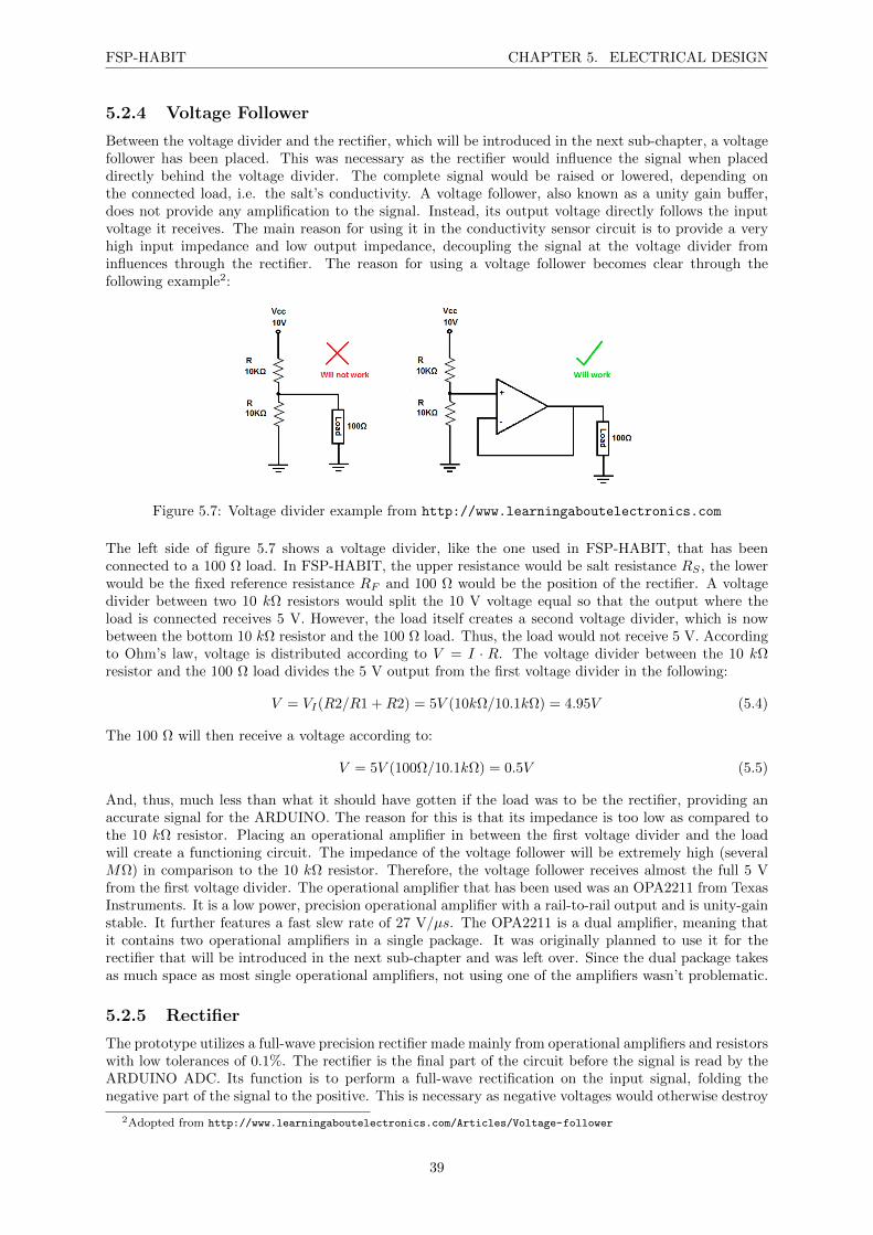
FSP-HABIT CHAPTER 5. ELECTRICAL DESIGN
5.2.4 Voltage Follower
Between the voltage divider and the rectifier, which will be introduced in the next sub-chapter, a voltagefollower has been placed. This was necessary as the rectifier would influence the signal when placeddirectly behind the voltage divider. The complete signal would be raised or lowered, depending onthe connected load, i.e. the salt’s conductivity. A voltage follower, also known as a unity gain buffer,does not provide any amplification to the signal. Instead, its output voltage directly follows the inputvoltage it receives. The main reason for using it in the conductivity sensor circuit is to provide a veryhigh input impedance and low output impedance, decoupling the signal at the voltage divider frominfluences through the rectifier. The reason for using a voltage follower becomes clear through thefollowing example2:
Figure 5.7: Voltage divider example from http://www.learningaboutelectronics.com
The left side of figure 5.7 shows a voltage divider, like the one used in FSP-HABIT, that has beenconnected to a 100 Ω load. In FSP-HABIT, the upper resistance would be salt resistance RS , the lowerwould be the fixed reference resistance RF and 100 Ω would be the position of the rectifier. A voltagedivider between two 10 kΩ resistors would split the 10 V voltage equal so that the output where theload is connected receives 5 V. However, the load itself creates a second voltage divider, which is nowbetween the bottom 10 kΩ resistor and the 100 Ω load. Thus, the load would not receive 5 V. Accordingto Ohm’s law, voltage is distributed according to V = I · R. The voltage divider between the 10 kΩresistor and the 100 Ω load divides the 5 V output from the first voltage divider in the following:
V = VI(R2/R1 +R2) = 5V (10kΩ/10.1kΩ) = 4.95V (5.4)
The 100 Ω will then receive a voltage according to:
V = 5V (100Ω/10.1kΩ) = 0.5V (5.5)
And, thus, much less than what it should have gotten if the load was to be the rectifier, providing anaccurate signal for the ARDUINO. The reason for this is that its impedance is too low as compared tothe 10 kΩ resistor. Placing an operational amplifier in between the first voltage divider and the loadwill create a functioning circuit. The impedance of the voltage follower will be extremely high (severalMΩ) in comparison to the 10 kΩ resistor. Therefore, the voltage follower receives almost the full 5 Vfrom the first voltage divider. The operational amplifier that has been used was an OPA2211 from TexasInstruments. It is a low power, precision operational amplifier with a rail-to-rail output and is unity-gainstable. It further features a fast slew rate of 27 V/µs. The OPA2211 is a dual amplifier, meaning thatit contains two operational amplifiers in a single package. It was originally planned to use it for therectifier that will be introduced in the next sub-chapter and was left over. Since the dual package takesas much space as most single operational amplifiers, not using one of the amplifiers wasn’t problematic.
5.2.5 Rectifier
The prototype utilizes a full-wave precision rectifier made mainly from operational amplifiers and resistorswith low tolerances of 0.1%. The rectifier is the final part of the circuit before the signal is read by theARDUINO ADC. Its function is to perform a full-wave rectification on the input signal, folding thenegative part of the signal to the positive. This is necessary as negative voltages would otherwise destroy
2Adopted from http://www.learningaboutelectronics.com/Articles/Voltage-follower
39
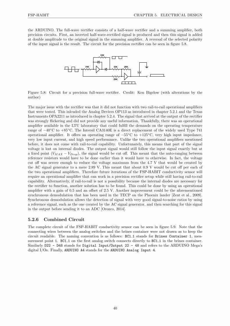
FSP-HABIT CHAPTER 5. ELECTRICAL DESIGN
the ARDUINO. The full-wave rectifier consists of a half-wave rectifier and a summing amplifier, bothprecision circuits. First, an inverted half-wave-rectified signal is produced and then this signal is addedat double amplitude to the original signal in the summing amplifier. A reversal of the selected polarityof the input signal is the result. The circuit for the precision rectifier can be seen in figure 5.8.
Figure 5.8: Circuit for a precision full-wave rectifier. Credit: Ken Bigelow (with alterations by theauthor)
The major issue with the rectifier was that it did not function with two rail-to-rail operational amplifiersthat were tested. This inlcuded the Analog Devices OP113 as introduced in chapter 5.2.1 and the TexasInstruments OPA2211 as introduced in chapter 5.2.4. The signal that arrived at the output of the rectifierwas strongly flickering and did not provide any useful information. Thankfully, there was an operationalamplifier available in the LTU laboratory that could fulfill the demands on the operating temperaturerange of −40C to +85C. The Intersil CA3140E is a direct replacement of the widely used Type 741operational amplifier. It offers an operating range of −55C to +125C, very high input impedance,very low input current, and high speed performance. Unlike the two operational amplifiers mentionedbefore, it does not come with rail-to-rail capability. Unfortunately, this means that part of the signalvoltage is lost on internal diodes. The output signal would still follow the input signal exactly but ata fixed point (VMAX − VDrop), the signal would be cut off. This meant that the auto-ranging betweenreference resistors would have to be done earlier than it would have to otherwise. In fact, the voltagecut off was severe enough to reduce the voltage maximum from the 4.7 V that would be created bythe AC signal generator to a mere 2.89 V. This meant that about 0.9 V would be cut off per each ofthe two operational amplifiers. Therefore future iterations of the FSP-HABIT conductivity sensor willrequire an operational amplifier that can work in a precision rectifier setup while still having rail-to-railcapability. Alternatively, if rail-to-rail is not a possibility because the internal diodes are necessary forthe rectifier to function, another solution has to be found. This could be done by using an operationalamplifier with a gain of 0.5 and an offset of 2.5 V. Another improvement could be the aforementionedsynchronous demodulation that has been used in the TECP on the Phoenix lander [Zent et al., 2009].Synchronous demodulation allows the detection of signal with very good signal-to-noise ratios by usinga reference signal, such as the one created by the AC signal generator, and then searching for this signalin the output before sending it to an ADC [Orozco, 2014].
5.2.6 Combined Circuit
The complete circuit of the FSP-HABIT conductivity sensor can be seen in figure 5.9. Note that theconnecting wires between the analog switches and the brines container were not drawn as to keep thecircuit readable. The naming convention is as follows: BC1 1 stands for Brines Container 1, mea-surement point 1. BC1 1 on the first analog switch connects directly to BC1 1 in the brines container.Similarly D22 - D48 stands for Digital Input/Output 22 - 48 and refers to the ARDUINO Mega’sdigital I/Os. Finally, ARDUINO A4 stands for the ARDUINO Analog Input 4.
40
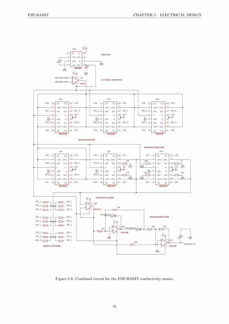
FSP-HABIT CHAPTER 5. ELECTRICAL DESIGN
4M
1M
100k
10k
1k
100
BC1_1BC1_2BC1_3
BC2_1BC2_2BC2_3
BC3_1BC3_2BC3_3
+-
+V
-V
+-
+V
-V
+-
+V
-V
+-
+V
-V
GNDGND
GND
VCC
VCC
VCC
VCC
VCC
GND
GND GND
GND GND
GND
VCC
VCC VCC VCC
VCC VCC
GND
GND
GND
GND
GND
GND
1N4148DO35-7
1N4148DO35-7
GND
GND
GND
ARDUINO PWM 1ARDUINO PWM 2
BC1_2
BC1_1 BC1_3
BC2_1
BC2_2
BC2_3
BC3_1
BC3_2
BC3_3
BC4_1
BC4_2
BC4_3
BC5_1
BC5_2
BC5_3
BC6_1
BC6_2
BC6_3
BC4_1BC4_2BC4_3
BC5_1BC5_2BC5_3
BC6_1BC6_2BC6_3
D30
D31
D28
D29
D32
D33
D34
D35
D36
D37
D38
D39
D40
D41
D42
D43
D44
D45
D22
D23
D24
D25
D26
D27
ARDUINO A4
10k
10k 10k
20k
20k
U$132 6
47
FC1CAP+2GND3CAP-4
V+ 8OSC 7
LV 6OUT 5
U$2
IN11COM12NO13V-4GND5NO46COM47IN48
IN2 16COM2 15
NO2 14V+ 13VL 12
NO3 11COM3 10
IN3 9
U$3IN11COM12NO13V-4GND5NO46COM47IN48
IN2 16COM2 15
NO2 14V+ 13VL 12
NO3 11COM3 10
IN3 9
U$4IN11COM12NO13V-4GND5NO46COM47IN48
IN2 16COM2 15
NO2 14V+ 13VL 12
NO3 11COM3 10
IN3 9
U$5
IN11COM12NO13V-4GND5NO46COM47IN48
IN2 16COM2 15
NO2 14V+ 13VL 12
NO3 11COM3 10
IN3 9
U$6IN11COM12NO13V-4GND5NO46COM47IN48
IN2 16COM2 15
NO2 14V+ 13VL 12
NO3 11COM3 10
IN3 9
U$7IN11COM12NO13V-4GND5NO46COM47IN48
IN2 16COM2 15
NO2 14V+ 13VL 12
NO3 11COM3 10
IN3 9
U$8
U$932 1
48
U$1032 6
47
U$1132 6
47
C1C2
D1
D2
C3
INVERTER
AC SIGNAL GENERATOR
ANALOG SWITCHES
REFERENCE RESISTORS
BRINES CONTAINER
VOLTAGE FOLLOWER
PRECISION RECTIFIER
OP113
ADM660
MAX4678 MAX4678 MAX4678
MAX4678 MAX4678 MAX4678
OPA2211
CA3140E
CA3140E
Figure 5.9: Combined circuit for the FSP-HABIT conductivity sensor.
41
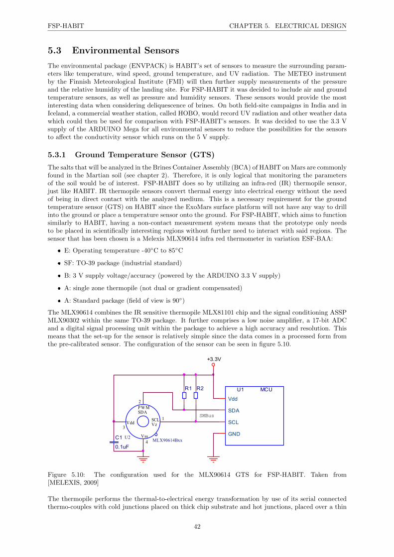
FSP-HABIT CHAPTER 5. ELECTRICAL DESIGN
5.3 Environmental Sensors
The environmental package (ENVPACK) is HABIT’s set of sensors to measure the surrounding param-eters like temperature, wind speed, ground temperature, and UV radiation. The METEO instrumentby the Finnish Meteorological Institute (FMI) will then further supply measurements of the pressureand the relative humidity of the landing site. For FSP-HABIT it was decided to include air and groundtemperature sensors, as well as pressure and humidity sensors. These sensors would provide the mostinteresting data when considering deliquescence of brines. On both field-site campaigns in India and inIceland, a commercial weather station, called HOBO, would record UV radiation and other weather datawhich could then be used for comparison with FSP-HABIT’s sensors. It was decided to use the 3.3 Vsupply of the ARDUINO Mega for all environmental sensors to reduce the possibilities for the sensorsto affect the conductivity sensor which runs on the 5 V supply.
5.3.1 Ground Temperature Sensor (GTS)
The salts that will be analyzed in the Brines Container Assembly (BCA) of HABIT on Mars are commonlyfound in the Martian soil (see chapter 2). Therefore, it is only logical that monitoring the parametersof the soil would be of interest. FSP-HABIT does so by utilizing an infra-red (IR) thermopile sensor,just like HABIT. IR thermopile sensors convert thermal energy into electrical energy without the needof being in direct contact with the analyzed medium. This is a necessary requirement for the groundtemperature sensor (GTS) on HABIT since the ExoMars surface platform will not have any way to drillinto the ground or place a temperature sensor onto the ground. For FSP-HABIT, which aims to functionsimilarly to HABIT, having a non-contact measurement system means that the prototype only needsto be placed in scientifically interesting regions without further need to interact with said regions. Thesensor that has been chosen is a Melexis MLX90614 infra red thermometer in variation ESF-BAA:
E: Operating temperature -40C to 85C
SF: TO-39 package (industrial standard)
B: 3 V supply voltage/accuracy (powered by the ARDUINO 3.3 V supply)
A: single zone thermopile (not dual or gradient compensated)
A: Standard package (field of view is 90)
The MLX90614 combines the IR sensitive thermopile MLX81101 chip and the signal conditioning ASSPMLX90302 within the same TO-39 package. It further comprises a low noise amplifier, a 17-bit ADCand a digital signal processing unit within the package to achieve a high accuracy and resolution. Thismeans that the set-up for the sensor is relatively simple since the data comes in a processed form fromthe pre-calibrated sensor. The configuration of the sensor can be seen in figure 5.10.
SCLVzVdd
R2
2
C1
0.1uF
3
U1 MCU
SCL
SDA
GND
Vdd
4
+3.3V
PWMSDA
U2MLX90614Bxx
R1
1SMBus
Vss
Figure 5.10: The configuration used for the MLX90614 GTS for FSP-HABIT. Taken from[MELEXIS, 2009]
The thermopile performs the thermal-to-electrical energy transformation by use of its serial connectedthermo-couples with cold junctions placed on thick chip substrate and hot junctions, placed over a thin
42
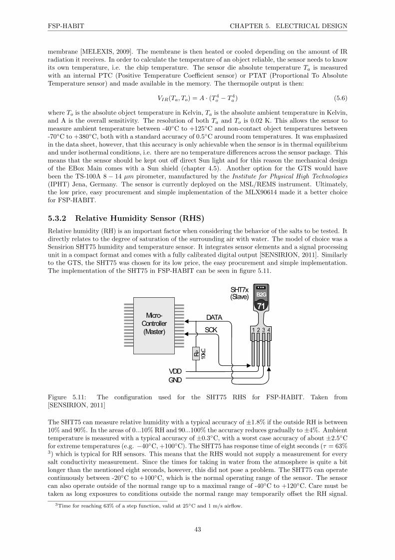
FSP-HABIT CHAPTER 5. ELECTRICAL DESIGN
membrane [MELEXIS, 2009]. The membrane is then heated or cooled depending on the amount of IRradiation it receives. In order to calculate the temperature of an object reliable, the sensor needs to knowits own temperature, i.e. the chip temperature. The sensor die absolute temperature Ta is measuredwith an internal PTC (Positive Temperature Coefficient sensor) or PTAT (Proportional To AbsoluteTemperature sensor) and made available in the memory. The thermopile output is then:
VIR(Ta, To) = A · (T 4o − T 4
a ) (5.6)
where To is the absolute object temperature in Kelvin, Ta is the absolute ambient temperature in Kelvin,and A is the overall sensitivity. The resolution of both Ta and To is 0.02 K. This allows the sensor tomeasure ambient temperature between -40C to +125C and non-contact object temperatures between-70C to +380C, both with a standard accuracy of 0.5C around room temperatures. It was emphasizedin the data sheet, however, that this accuracy is only achievable when the sensor is in thermal equilibriumand under isothermal conditions, i.e. there are no temperature differences across the sensor package. Thismeans that the sensor should be kept out off direct Sun light and for this reason the mechanical designof the EBox Main comes with a Sun shield (chapter 4.5). Another option for the GTS would havebeen the TS-100A 8 − 14 µm pirometer, manufactured by the Institute for Physical High Technologies(IPHT) Jena, Germany. The sensor is currently deployed on the MSL/REMS instrument. Ultimately,the low price, easy procurement and simple implementation of the MLX90614 made it a better choicefor FSP-HABIT.
5.3.2 Relative Humidity Sensor (RHS)
Relative humidity (RH) is an important factor when considering the behavior of the salts to be tested. Itdirectly relates to the degree of saturation of the surrounding air with water. The model of choice was aSensirion SHT75 humidity and temperature sensor. It integrates sensor elements and a signal processingunit in a compact format and comes with a fully calibrated digital output [SENSIRION, 2011]. Similarlyto the GTS, the SHT75 was chosen for its low price, the easy procurement and simple implementation.The implementation of the SHT75 in FSP-HABIT can be seen in figure 5.11.
VDDGND
DATA
SCK
71
B2G
1 2 3 4
Micro- Controller (Master)
SHT7x(Slave)
RP
10kΩ
Figure 5.11: The configuration used for the SHT75 RHS for FSP-HABIT. Taken from[SENSIRION, 2011]
The SHT75 can measure relative humidity with a typical accuracy of ±1.8% if the outside RH is between10% and 90%. In the areas of 0...10% RH and 90...100% the accuracy reduces gradually to ±4%. Ambienttemperature is measured with a typical accuracy of ±0.3C, with a worst case accuracy of about ±2.5Cfor extreme temperatures (e.g. −40C, +100C). The SHT75 has response time of eight seconds (τ = 63%3) which is typical for RH sensors. This means that the RHS would not supply a measurement for everysalt conductivity measurement. Since the times for taking in water from the atmosphere is quite a bitlonger than the mentioned eight seconds, however, this did not pose a problem. The SHT75 can operatecontinuously between -20C to +100C, which is the normal operating range of the sensor. The sensorcan also operate outside of the normal range up to a maximal range of -40C to +120C. Care must betaken as long exposures to conditions outside the normal range may temporarily offset the RH signal.
3Time for reaching 63% of a step function, valid at 25C and 1 m/s airflow.
43
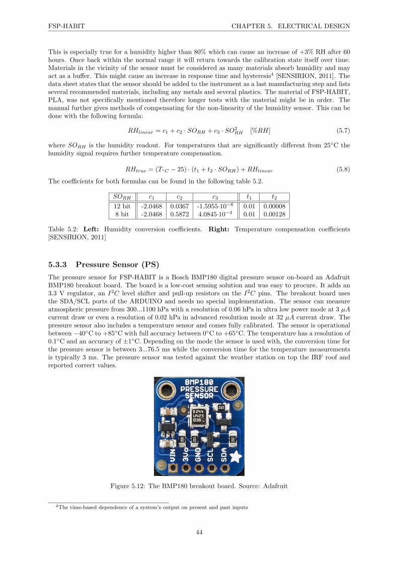
FSP-HABIT CHAPTER 5. ELECTRICAL DESIGN
This is especially true for a humidity higher than 80% which can cause an increase of +3% RH after 60hours. Once back within the normal range it will return towards the calibration state itself over time.Materials in the vicinity of the sensor must be considered as many materials absorb humidity and mayact as a buffer. This might cause an increase in response time and hysteresis4 [SENSIRION, 2011]. Thedata sheet states that the sensor should be added to the instrument as a last manufacturing step and listsseveral recommended materials, including any metals and several plastics. The material of FSP-HABIT,PLA, was not specifically mentioned therefore longer tests with the material might be in order. Themanual further gives methods of compensating for the non-linearity of the humidity sensor. This can bedone with the following formula:
RHlinear = c1 + c2 · SORH + c3 · SO2RH [%RH] (5.7)
where SORH is the humidity readout. For temperatures that are significantly different from 25C thehumidity signal requires further temperature compensation.
RHtrue = (TC − 25) · (t1 + t2 · SORH) +RHlinear (5.8)
The coefficients for both formulas can be found in the following table 5.2.
SORH c1 c2 c3 t1 t2
12 bit -2.0468 0.0367 -1.5955·10−6 0.01 0.000088 bit -2.0468 0.5872 4.0845·10−4 0.01 0.00128
Table 5.2: Left: Humidity conversion coefficients. Right: Temperature compensation coefficients[SENSIRION, 2011]
5.3.3 Pressure Sensor (PS)
The pressure sensor for FSP-HABIT is a Bosch BMP180 digital pressure sensor on-board an AdafruitBMP180 breakout board. The board is a low-cost sensing solution and was easy to procure. It adds an3.3 V regulator, an I2C level shifter and pull-up resistors on the I2C pins. The breakout board usesthe SDA/SCL ports of the ARDUINO and needs no special implementation. The sensor can measureatmospheric pressure from 300...1100 hPa with a resolution of 0.06 hPa in ultra low power mode at 3 µAcurrent draw or even a resolution of 0.02 hPa in advanced resolution mode at 32 µA current draw. Thepressure sensor also includes a temperature sensor and comes fully calibrated. The sensor is operationalbetween −40C to +85C with full accuracy between 0C to +65C. The temperature has a resolution of0.1C and an accuracy of ±1C. Depending on the mode the sensor is used with, the conversion time forthe pressure sensor is between 3...76.5 ms while the conversion time for the temperature measurementsis typically 3 ms. The pressure sensor was tested against the weather station on top the IRF roof andreported correct values.
Figure 5.12: The BMP180 breakout board. Source: Adafruit
4The time-based dependence of a system’s output on present and past inputs
44

FSP-HABIT CHAPTER 5. ELECTRICAL DESIGN
5.3.4 Air Temperature Sensor (ATS)
The sensors used for the ATS were three analog C420 Pt1000 sensors from Heraeus. The sensors cover atemperature range from −196C to +150C which is covering the operating temperature of FSP-HABITof −40C to +85C. The sensor comes with AgPd-wire leads of 15 mm and an accuracy of ±0.3C.Pt1000 sensors have a nominal resistance of 1000 Ω at 0C which then changes linearly with higheror lower temperatures. The C420 is characterized by high long-term stability (max. R0-Drift 0.03%after 1000 h at 150C), excellent temperature shock resistance and a minimal deviation from the DINEN 60751 (according to IEC 751) characteristic curve over the entire temperature range, showing nohysteresis. The Pt1000 sensors can be read out by simply arranging them in a voltage divider setupwith another 1000 Ω resistor. The resistance value of the Pt1000 can then be calculated to a precisionof 1.2C by:
R =R0
1023value − 1
(5.9)
Parallel to the development of FSP-HABIT another Master’s thesis was in works, carried out by PhilippWittmann, at the time member of the LTU atmospheric science group. The goal of the Master’s the-sis was the measurement of the convective heat transfer with wind. For this, Wittmann used threePt1000 sensors in combination with a circuit that increased the precision that was attainable with thesensors. As described in [Philipp Wittmann, 2016], the basic principle of the circuit used was takenfrom [Tietze and Schenk, 1991] and then improved with knowledge gained from [Trystan Lea, 2010]. Toincrease the precision of the sensor, the internal reference was set from 5 V to a lower value of 1.1 V.This was done as the measurement range is divided by the precision of the ARDUINO ADC which candistinguish between 1024 different values. Then 1.1V/1023 = 1.07mV which is smaller than the original5V/1023 = 4.89mV , meaning that differences of 1.07 mV could be distinguished. This led to an increasein sensor sensitivity up to 0.17
Cstep , four times the initial sensitivity.
Sensor calibration is then done with the help of two formulas:
RT = R0 · (1 +A · T +B · T 2) (5.10)
RT = R0 · [1 +A · T +B · T 2 + C · (T − 100C) · T 3] (5.11)
with
A = 3.9083 · 10−3 1C
B = −5.7750 · 10−7 1C2
C = −4.1830 · 10−12 1C4
Formula 5.10 is used for positive temperatures while formula 5.11 covers negative temperatures. Coef-ficients A, B, and C are constants, R0 the resistance of the Pt1000 at 0C (= 1000Ω), and RT is theresistance of the Pt1000 for a given temperature T . The circuit of the ATS is covered in more detailin [Philipp Wittmann, 2016] and has been used for FSP-HABIT as found there. Figure 5.13 shows thecircuit of the ATS in detail.
45

FSP-HABIT CHAPTER 5. ELECTRICAL DESIGN
Figure 5.13: Electrical circuit of the air temperature sensors (ATS). From [Philipp Wittmann, 2016]
5.4 Power System
FSP-HABIT is powered by eight AA batteries which are mounted in a battery holder of type BH48AASF.Due to travel regulations, the prototype used NiMH batteries instead of lithium batteries in Icelandand in India. This did increase the minimum operating temperature of the prototype to about −10Cinstead of the otherwise possible −40C. However, since the prototypes were used during summer, NiMHbatteries were sufficient for the tasks at hand. Assuming a worst-case scenario where the temperaturesare at −10C and the ARDUINO of the prototype draws its maximum of 200 mA while the mostpower consuming component, the SD card writer/reader, draws 100 mA, the prototype could run forapproximately 4.17 hours. This number assumes 2500 mAh batteries and a loss of about 50% in batterycapacitance due to the cold temperatures. The 50%-value has been taken from the figure 5.14. Thebattery compartment of FSP-HABIT has been designed with accessibilty in mind and the batteries areeasily replaced with batteries of AA shape. Switching to lithium batteries or accumulators is thereforepossible. Lithium batteries can be operated at far lower temperatures than NiMH which becomes clearwhen comparing figure 5.14 with figure 5.15. It can be seen that the NiMH battery loses as much as80% of its capacity at −20C while the lithium battery still retain at least two-thirds of its capacity atthe same temperature. A switching regulator of type TSR12450 replaced the ARDUINO default linearregulator which is not energy efficient in battery powered applications. The TSR12450 can provide upto 94% efficiency in converting DC to DC voltages without requiring a heat-sink. It can be operatedbetween −40C to +85C (up to +60C without the need for a heat-sink). According to the manufacturerTraco Power, the TSR-1 switching regulators provide significant advantages over linear regulators, i.e.better output accuracy (±2%), lower standby current of 2 mA and no requirement for external capacitors[POWER, 2016]. The switching regulator is connected with the battery Vcc, the battery and ARDUINOGNDs, and the ARDUINO 5 V input. Since FSP-HABIT is to be tested in different humidity conditions,it is important to note that TSR-1 switching regulators should not be used at relative humidity higher95% for anything but short time frames.
46
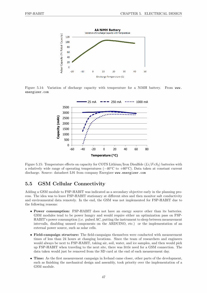
FSP-HABIT CHAPTER 5. ELECTRICAL DESIGN
Figure 5.14: Variation of discharge capacity with temperature for a NiMH battery. From www.
energizer.com
0
500
1000
1500
2000
2500
3000
3500
-60 -40 -20 0 20 40 60 80
Cap
acit
y (m
Ah
)
Temperature (°C)
25 mA 250 mA 1000 mA
Figure 5.15: Temperature effects on capacity for COTS Lithium/Iron Disulfide (Li/FeS2) batteries witha relatively wide range of operating temperatures (−40C to +60C). Data taken at constant currentdischarge. Source: datasheet L91 from company Energizer www.energizer.com
5.5 GSM Cellular Connectivity
Adding a GSM module to FSP-HABIT was indicated as a secondary objective early in the planning pro-cess. The idea was to leave FSP-HABIT stationary at different sites and then monitor salt conductivityand environmental data remotely. In the end, the GSM was not implemented for FSP-HABIT due tothe following reasons:
Power consumption: FSP-HABIT does not have an energy source other than its batteries.GSM modules tend to be power hungry and would require either an optimization pass on FSP-HABIT’s power consumption (i.e. pulsed AC, putting the instrument to sleep between measurementintervalls, disabling unused components on the ARDUINO, etc.) or the implementation of anexternal power source, such as solar cells.
Field-campaign structure: The field-campaigns themselves were conducted with measurementtimes of less than 24 hours at changing locations. Since the team of researchers and engineerswould always be next to FSP-HABIT, taking air, soil, water, and ice samples, and then would pickup FSP-HABIT when traveling to the next site, there was little need for a GSM connection. Thedata taken would just be removed from the SD card at the end of each measurement day.
Time: As the first measurement campaign in Iceland came closer, other parts of the development,such as finishing the mechanical design and assembly, took priority over the implementation of aGSM module.
47
FSP-HABIT CHAPTER 5. ELECTRICAL DESIGN
Several modules have been considered before the objective was dropped:
Thinking Things Open (TTOpen): TTOpen is currently offered as a beta program by theSpanish company Telefonica. Thinking Things is a system made for building Internet of Thingsdevices and connecting them to an open cloud service in the Internet. The beta program sup-plies the participants with a development board and an industrial module of Thinking ThingsOpen. The modules are free of charge, but in exchange the participants help in the evaluationprocess. TTOpen boards include a Telefonica SIM with mobile communications included for oneyear and use the ARDUINO IDE. TTOpen is already available in version one and soon avialable asTTOpen V2 (as described on http://www.thinkingthings.telefonica.com/beta/productos/).TTOpen V2 will have more capabilities as compared to the first version and uses a different micro-controller as compared to the ARDUINO Uno and the ARDUINO Mega. While the board wouldhave been free-of-charge, the extra-effort for evaluation, time for procurement, possible reliabilityissues, and the less capable development board than the ARDUINO Mega 2560 (e.g. pin count forV1 severely lower, comparable to ARDUINO Uno with V2) could have negatively impacted thedevelopment.
ARDUINO GSM Shield: As an alternative to TTOpen, the commercially available ARDUINOGSM Shield could have been used for cellular connectivity. The Arduino GSM Shield allowsan ARDUINO board to connect to the internet, make/receive voice calls and send/receive SMSmessages. To interface with the cellular network, the board requires a SIM card provided by anetwork operator. During the time of consideration, the GSM Shield was readily available, camewith good documentation, and a possibly higher reliability than the TTOpen beta. The GSMShield has been retired by now, however, and would have come with high power demands (themanufacturer recommendeds that the board is powered with an external power supply that canprovide between 700 mA and 1000 mA) and a bulky form factor (about same size as ARDUINOMega 2560, mounted on top of the ARDUINO).
Adafruit FONA: FONA describes a product line from supplier Adafruit that can be bought indifferent variations. The Adafruit FONA MiniGSM combines a small package with quad-band850/900/1800/1900MHz GSM which can connect to 2G networks all over the globe (as some of theFONA variations are location-bound). Its main downside is, as with the other options, the needfor an external battery. Adafruit recommends a LiPoly battery charging circuitry with at least 500mAh. The FONA also requires a 2G mini SIM card which can be hard to find since some cellularnetwork providers no longer produce 2G cards. The use of 2G technology also means that theconnection speed of the FONA MiniGSM is fairly limited. 3G versions of the FONA are available(e.g. Adafruit FONA 3G Cellular Breakout - European version) but, according to Adafruit, areideally used with a 1200 mAh battery and the data functionality is not as easy to use. Adafruitis currently adapting its FONA library to support the 3G chipset which currently supports SMS,calling, and basic functionality but does not yet support full GPRS TCP/IP and HTTP support.
5.6 SD Card Reader
For data storage, FSP-HABIT has a MicroSD card breakout board+ from supplier Adafruit installed.The board is found in the EBox Lid and provides an easy method of writing to and reading from aMicroSD card. Using a SD card can require a lot of data transfer. According to the supplier, the cardreader should therefore be connected up to the hardware Serial Peripheral Interface (SPI) pins of amicrocontroller (instead of to an interface like I2C). The reader was then powered with the 3.3 V supplyand installed to the ARDUINO digital pins 50 (MISO: Master Input, Slave Output), 51 (MOSI: MasterOutput, Slave Input), 52 (SCK: Serial Clock), and 53 (CS: Chip Select).
48
Chapter 6
Software
The software for FSP-HABIT was written in the ARDUINO Integrated Development Environment(IDE), provided by www.arduino.org1 in version 1.7.11. The ARDUINO IDE contains an editorfor writing code, several debugging tools and common functions. Programs written in the IDE arecalled sketches and realized in the ARDUINO programming language. The website of ARDUINO LLC(https://www.arduino.cc/en/Main/FAQ) states that the Arduino language is a set of C/C++ functionsthat can be called from the code. The sketch undergoes minor changes (e.g. automatic generation offunction prototypes) and then is passed directly to a C/C++ compiler (avr-g++). The approach for theenvironmental sensors (chapter 5.3) was similar for each sensor: pre-existing libraries and examplecode were first put into a separate sketch for each sensor. Whenever needed, the example code wasaltered to fit FSP-HABIT’s demands. The following has been used:
GTS: For the MELEXIS MLX90614 ESF-BAA, a tutorial from electronics supplier Adafruit hasbeen used:https://learn.adafruit.com/using-melexis-mlx90614-non-contact-sensors/wiring-and-
test. Adafruit offers a library written for the sensor and a corresponding demo. The library canbe found at https://github.com/adafruit/Adafruit-MLX90614-Library. Once the library hasbeen added to the ARDUINO IDE by simply copying the downloaded files to the right repository,the demo will then be found within the ARDUINO IDE under File → Examples → AdafruitMLX90614→ mlxtest.
RHS: For the SENSIRION SHT75, a library and a corresponding example was found inside theARDUINO playground, a website run by ARDUINO LLC where the users of Arduino can contributeand benefit from their collective research. The website can be found at http://playground.
arduino.cc/Code/Sensirion#Example, the library for SENSIRION SHT1x and SHT7x sensorswas originally created by Markus Schatzl in 2008 with a revision and then a rewrite by CarlJackson in 2010.
PS: The Bosch BMP180 is sold as a complete package by Adafruit as the BMP180 BarometricPressure/Temperature/Altitude Sensor breakout board. The company also provides a tutorial anda library for the setup of the sensor. The library can be used by both the BMP180 breakoutboard, as well as its predecessor, the BMP85. The library can be found at https://github.com/adafruit/Adafruit_BMP085_Unified while the tutorial is found at https://learn.adafruit.
com/bmp085/using-the-bmp085-api-v2. Additionally to the BMP085 library, the Adafruit Uni-fied Sensor Library (USL) is also needed for the breakout board to function with the code given inthe tutorial. The USL provides a common interface and data type for sensors purchased throughsupplier Adafruit. According to Adafruit, it defines some basic information about the sensor (sen-sor limits, etc.), and returns standard SI units of a specific type and scale for each supported sensortype. The USL can be found at https://github.com/adafruit/Adafruit_Sensor.
ATS: The code for the Pt1000 sensors and the corresponding circuit was developed by[Philipp Wittmann, 2016] and references therein. The code was provided to FSP-HABIT as asketch for the ARDUINO IDE and later incorporated into the FSP-HABIT main program.
1Two different companies use the ARDUINO name, ARDUINO LLC which runs www.arduino.cc and ARDUINO SRL(formerly known as Smart Projects SRL) which runs www.arduino.org. The two companies provide similar products buthave their own development branches and provide slightly different IDEs. In 2015 a lawsuit at the Massachusetts DistrictCourt was started between both companies.
49
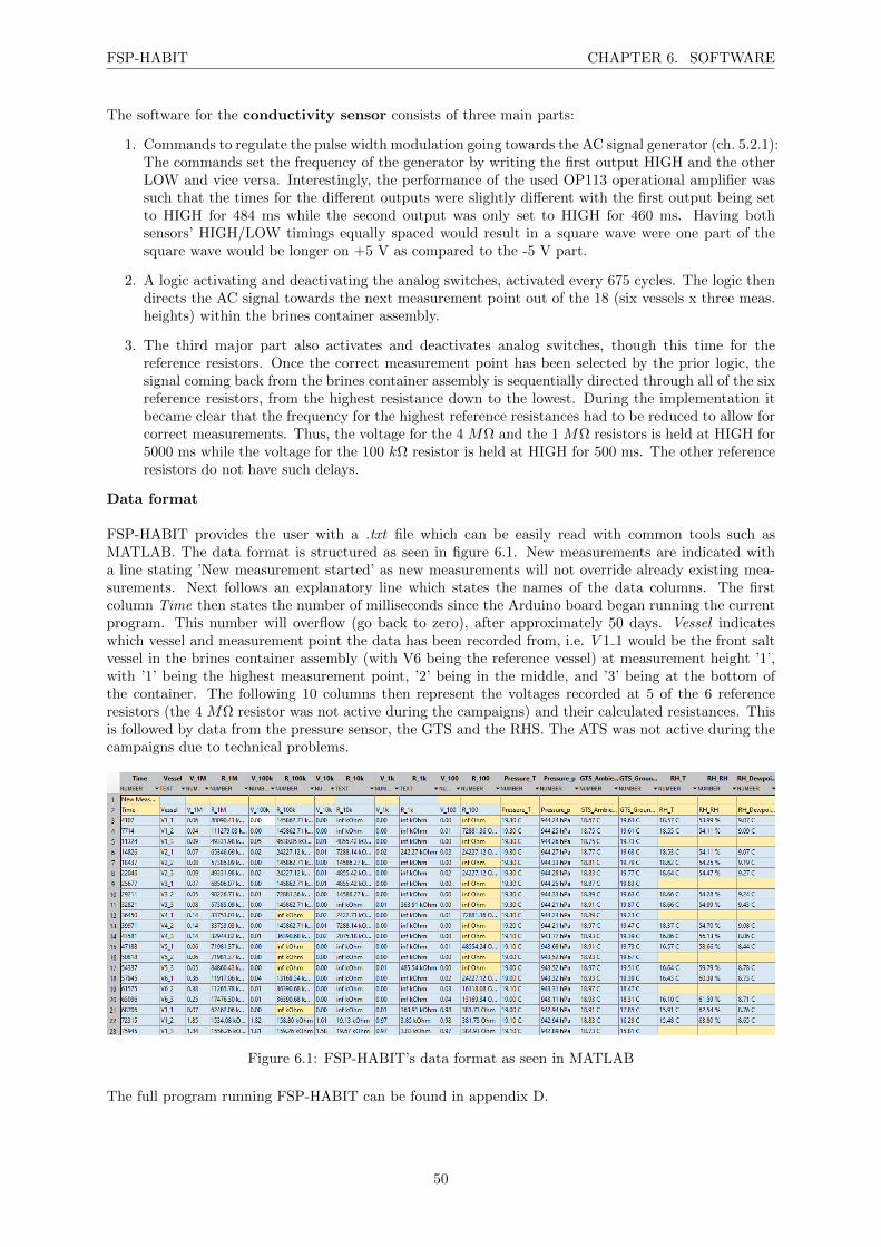
FSP-HABIT CHAPTER 6. SOFTWARE
The software for the conductivity sensor consists of three main parts:
1. Commands to regulate the pulse width modulation going towards the AC signal generator (ch. 5.2.1):The commands set the frequency of the generator by writing the first output HIGH and the otherLOW and vice versa. Interestingly, the performance of the used OP113 operational amplifier wassuch that the times for the different outputs were slightly different with the first output being setto HIGH for 484 ms while the second output was only set to HIGH for 460 ms. Having bothsensors’ HIGH/LOW timings equally spaced would result in a square wave were one part of thesquare wave would be longer on +5 V as compared to the -5 V part.
2. A logic activating and deactivating the analog switches, activated every 675 cycles. The logic thendirects the AC signal towards the next measurement point out of the 18 (six vessels x three meas.heights) within the brines container assembly.
3. The third major part also activates and deactivates analog switches, though this time for thereference resistors. Once the correct measurement point has been selected by the prior logic, thesignal coming back from the brines container assembly is sequentially directed through all of the sixreference resistors, from the highest resistance down to the lowest. During the implementation itbecame clear that the frequency for the highest reference resistances had to be reduced to allow forcorrect measurements. Thus, the voltage for the 4 MΩ and the 1 MΩ resistors is held at HIGH for5000 ms while the voltage for the 100 kΩ resistor is held at HIGH for 500 ms. The other referenceresistors do not have such delays.
Data format
FSP-HABIT provides the user with a .txt file which can be easily read with common tools such asMATLAB. The data format is structured as seen in figure 6.1. New measurements are indicated witha line stating ’New measurement started’ as new measurements will not override already existing mea-surements. Next follows an explanatory line which states the names of the data columns. The firstcolumn Time then states the number of milliseconds since the Arduino board began running the currentprogram. This number will overflow (go back to zero), after approximately 50 days. Vessel indicateswhich vessel and measurement point the data has been recorded from, i.e. V 1 1 would be the front saltvessel in the brines container assembly (with V6 being the reference vessel) at measurement height ’1’,with ’1’ being the highest measurement point, ’2’ being in the middle, and ’3’ being at the bottom ofthe container. The following 10 columns then represent the voltages recorded at 5 of the 6 referenceresistors (the 4 MΩ resistor was not active during the campaigns) and their calculated resistances. Thisis followed by data from the pressure sensor, the GTS and the RHS. The ATS was not active during thecampaigns due to technical problems.
Figure 6.1: FSP-HABIT’s data format as seen in MATLAB
The full program running FSP-HABIT can be found in appendix D.
50

Part III
RESULTS
51
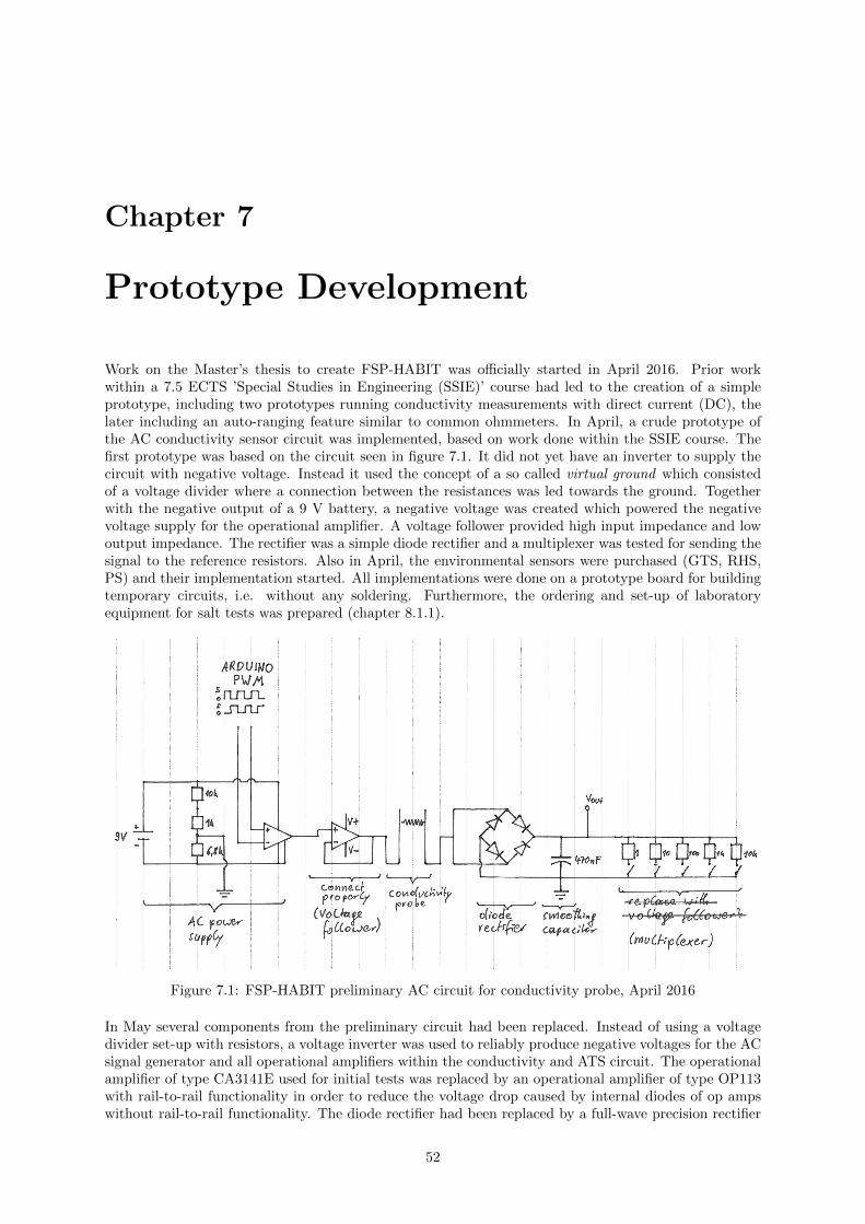
Chapter 7
Prototype Development
Work on the Master’s thesis to create FSP-HABIT was officially started in April 2016. Prior workwithin a 7.5 ECTS ’Special Studies in Engineering (SSIE)’ course had led to the creation of a simpleprototype, including two prototypes running conductivity measurements with direct current (DC), thelater including an auto-ranging feature similar to common ohmmeters. In April, a crude prototype ofthe AC conductivity sensor circuit was implemented, based on work done within the SSIE course. Thefirst prototype was based on the circuit seen in figure 7.1. It did not yet have an inverter to supply thecircuit with negative voltage. Instead it used the concept of a so called virtual ground which consistedof a voltage divider where a connection between the resistances was led towards the ground. Togetherwith the negative output of a 9 V battery, a negative voltage was created which powered the negativevoltage supply for the operational amplifier. A voltage follower provided high input impedance and lowoutput impedance. The rectifier was a simple diode rectifier and a multiplexer was tested for sending thesignal to the reference resistors. Also in April, the environmental sensors were purchased (GTS, RHS,PS) and their implementation started. All implementations were done on a prototype board for buildingtemporary circuits, i.e. without any soldering. Furthermore, the ordering and set-up of laboratoryequipment for salt tests was prepared (chapter 8.1.1).
Figure 7.1: FSP-HABIT preliminary AC circuit for conductivity probe, April 2016
In May several components from the preliminary circuit had been replaced. Instead of using a voltagedivider set-up with resistors, a voltage inverter was used to reliably produce negative voltages for the ACsignal generator and all operational amplifiers within the conductivity and ATS circuit. The operationalamplifier of type CA3141E used for initial tests was replaced by an operational amplifier of type OP113with rail-to-rail functionality in order to reduce the voltage drop caused by internal diodes of op ampswithout rail-to-rail functionality. The diode rectifier had been replaced by a full-wave precision rectifier
52
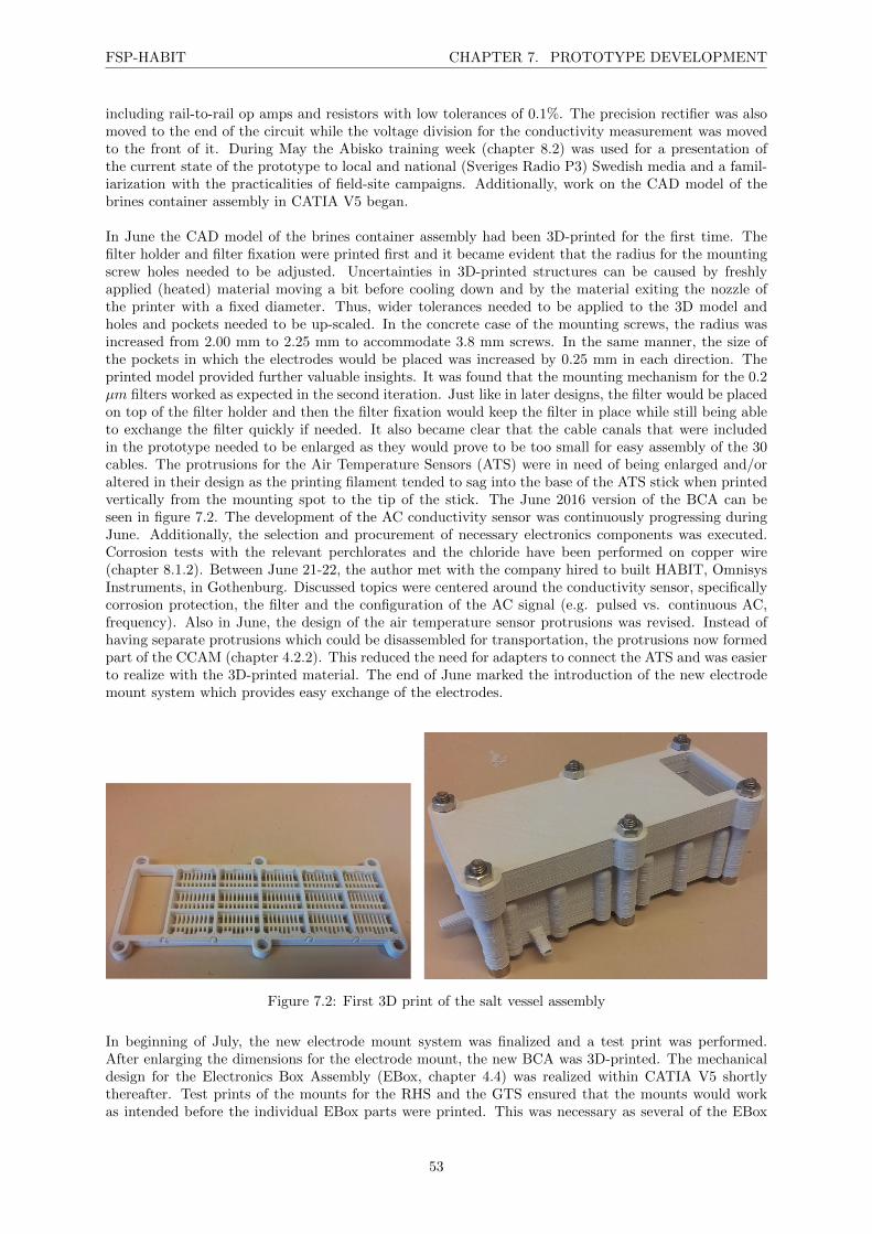
FSP-HABIT CHAPTER 7. PROTOTYPE DEVELOPMENT
including rail-to-rail op amps and resistors with low tolerances of 0.1%. The precision rectifier was alsomoved to the end of the circuit while the voltage division for the conductivity measurement was movedto the front of it. During May the Abisko training week (chapter 8.2) was used for a presentation ofthe current state of the prototype to local and national (Sveriges Radio P3) Swedish media and a famil-iarization with the practicalities of field-site campaigns. Additionally, work on the CAD model of thebrines container assembly in CATIA V5 began.
In June the CAD model of the brines container assembly had been 3D-printed for the first time. Thefilter holder and filter fixation were printed first and it became evident that the radius for the mountingscrew holes needed to be adjusted. Uncertainties in 3D-printed structures can be caused by freshlyapplied (heated) material moving a bit before cooling down and by the material exiting the nozzle ofthe printer with a fixed diameter. Thus, wider tolerances needed to be applied to the 3D model andholes and pockets needed to be up-scaled. In the concrete case of the mounting screws, the radius wasincreased from 2.00 mm to 2.25 mm to accommodate 3.8 mm screws. In the same manner, the size ofthe pockets in which the electrodes would be placed was increased by 0.25 mm in each direction. Theprinted model provided further valuable insights. It was found that the mounting mechanism for the 0.2µm filters worked as expected in the second iteration. Just like in later designs, the filter would be placedon top of the filter holder and then the filter fixation would keep the filter in place while still being ableto exchange the filter quickly if needed. It also became clear that the cable canals that were includedin the prototype needed to be enlarged as they would prove to be too small for easy assembly of the 30cables. The protrusions for the Air Temperature Sensors (ATS) were in need of being enlarged and/oraltered in their design as the printing filament tended to sag into the base of the ATS stick when printedvertically from the mounting spot to the tip of the stick. The June 2016 version of the BCA can beseen in figure 7.2. The development of the AC conductivity sensor was continuously progressing duringJune. Additionally, the selection and procurement of necessary electronics components was executed.Corrosion tests with the relevant perchlorates and the chloride have been performed on copper wire(chapter 8.1.2). Between June 21-22, the author met with the company hired to built HABIT, OmnisysInstruments, in Gothenburg. Discussed topics were centered around the conductivity sensor, specificallycorrosion protection, the filter and the configuration of the AC signal (e.g. pulsed vs. continuous AC,frequency). Also in June, the design of the air temperature sensor protrusions was revised. Instead ofhaving separate protrusions which could be disassembled for transportation, the protrusions now formedpart of the CCAM (chapter 4.2.2). This reduced the need for adapters to connect the ATS and was easierto realize with the 3D-printed material. The end of June marked the introduction of the new electrodemount system which provides easy exchange of the electrodes.
Figure 7.2: First 3D print of the salt vessel assembly
In beginning of July, the new electrode mount system was finalized and a test print was performed.After enlarging the dimensions for the electrode mount, the new BCA was 3D-printed. The mechanicaldesign for the Electronics Box Assembly (EBox, chapter 4.4) was realized within CATIA V5 shortlythereafter. Test prints of the mounts for the RHS and the GTS ensured that the mounts would workas intended before the individual EBox parts were printed. This was necessary as several of the EBox
53

FSP-HABIT CHAPTER 7. PROTOTYPE DEVELOPMENT
parts took around 24 hours to print (specifically, the EBox Main an the EBox Lid). Problems withthe 3D-printer, such as a cutting of the material feeder into the filament with a subsequent cut-off inthe supplied material and filament getting stuck in the nozzle of the printer caused several re-prints.Meanwhile, the assembly of the prototype as a whole began. The electrical components were solderedonto a 160 x 100 [mm] circuit board of type EuroCard. Using an etched circuit board or a printed circuitboard would have been alternatives for the EuroCard. However, the time for assembling the prototypewas limited and it was deemed that if the etched or printed circuit boards had contained errors, thetime left for assembly would have been too short. The EuroCard approach came with its own problems,namely the poor clarity and easy creation of overlapping soldering points. These difficulties ultimatelyled to the ATS circuit not functioning. Since the GTS, RHS, and PS had their own air temperaturesensors included, it was decided to forego the ATS and use the data from the other sensors instead. TheATS sensors and circuit are found within the prototype but would need debugging to function. Theassembly then consisted of all necessary soldering, wiring, gluing, and fixations. Between July 16-25, theauthor and the prototype were in Iceland to perform tests with the prototype (chapter 8.3). BetweenJuly 27-28, a problem with the ARDUINO necessitated a two-day fixing period. The digital I/Os ofthe ARDUINO were not capable of providing a proper HIGH/LOW signal for all of the connected 24switches. A small circuit board with pull up resistors was included to fix the problem. On, July 29 theprototype was packed for the India campaign which ran from August 7-19.
Figure 7.3: Iterations of the BCA.
Figure 7.4: FSP-HABIT during preparation for the India campaign
54
Chapter 8
Testing
8.1 Laboratory Salt Tests
8.1.1 Preparation
Several preparatory actions have been performed before work with the perchlorates and the chloridewas started. On April 11, Dr. Hans Karlstrom, CEO of LKAB Kimit AB gave a lecture on the topic.LKAB Kimit AB are the manufacturers of the explosives used in the world’s largest underground iron oremine, run by Luossavaara-Kiirunavaara AB (LKAB). Dr. Karlstrom’s lecture covered information aboutoxidizers in general, and specifically focused on the substances manipulated within the HABIT, FSP-HABIT and SALACIA projects. The perchlorate and chloride Material Safety Data Sheets (MSDS)were studied for each component and a list of laboratory equipment was prepared. The equipmentwas then ordered during April. From the MSDS, a risk analysis was performed by Martin Svenssonof SALACIA. This was followed up by a visit of the SALACIA REXUS science team, including theauthor, and LTU personnel to the facilities of Kimit on May 29. The delegation received training inthe handling of oxidizers within Kimit’s laboratories from industry experts Viktoria Klippmark andLars Jonasson. In their laboratories, the delegation was taught about the correct handling of oxidizers,how to work efficiently and safe in a laboratory, how to handle emergencies and was able to ask veryspecific questions. The Kimit staff checked the risk analysis conducted for the LTU laboratory andgave valuable comments. The visit was concluded with a factory tour. On May 1, an inspection of theLTU laboratories was conducted by Ms. Klippmark, including a check of the students procedures whenhandling perchlorates.
8.1.2 Corrosion Tests, June 2016
In June 2016, one remaining question was which material should be used for the electrodes. The designforesaw small, rectangular, metal sheets which would provide clear geometrical outlines. The metalsheets were then to be soldered with a wire on one side, with the other side being in contact with thesalts. Glue for marine applications would hold the sheets in place. Due to the electrolysis happeningduring the AC measurements, there was a concern that the plates would corrode during the time of lifeof the prototype. It was unknown, however, to what degree a possible corrosive effect would actuallymanifest itself due the unusual combination of low voltage (smaller 5 V) and relatively high frequenciesof 9-10 kHz. Several materials were considered: pure copper, pure gold, pure platinum, and gold platedcopper.
Copper represented the cheapest alternative and would therefore be preferred.
Gold is chemically inert and would be a good but pricey choice.
Platinum is chemically inert like gold but hard to work with.
Gold platted copper would be cheaper than pure gold but would introduce uncertainties as it wouldbe difficult to determine how the different materials influence the conductivity measurement. Thisis especially true when it is considered that nickel is needed between the gold and the copper toconnect the two materials. For AC measurements this material mix could also create a capacitivecoupling between the different materials although the high frequency of 9-10 kHz should counteractthis.
55

FSP-HABIT CHAPTER 8. TESTING
Gold platted copper was ruled out early on because of the reasons stated above. The preferred materialwas pure copper. It would represent the cheapest choice but also the choice with the highest likelihoodfor corrosion. To determine if copper was a possible choice, several tests were performed. These testsconsisted of a simple setup with two copper wires, table salt and tap water. The wires were bend intoa small 5 ml beaker and then connected to a multimeter and a signal generator which provided thefollowing values:
Test 1: ±4 V / 9.3 kHz / 7.10 mA, 5 hours of test
Test 2: ±5 V / 9.3 kHz V 8.8 mA, 4 hours of test. Wires prepared with sand paper to removepossible coating of the copper wires.
After the test, the salt water was inspected for possible changes of color and the wires were checked forsigns of corrosion visually. The result in both cases was that no indications of corrosion were detected.Figure 8.1 shows the setup and the results of the corrosion tests.
Figure 8.1: Top left: Test setup with multimeter, salt vessel, signal generator; Bottom left: O2 andH2 bubbles due to electrolysis; Middle: Beaker with salt-water solution after test. No visible change incolor. ’Climbing’ of the salts along the wet walls; Right: Copper wires after test. The third, straight,wire was used for comparison and wasn’t subjected to the salt-water solution and AC.
Figure 8.2: Copper wires after being tested with the perchlorates: Left: Calcium perchlorate Middle:Magnesium perchlorate Right: Sodium perchlorate
56
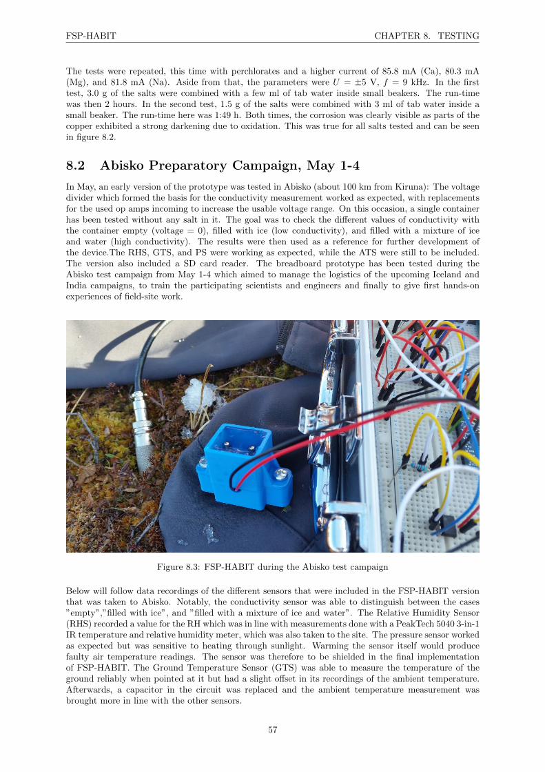
FSP-HABIT CHAPTER 8. TESTING
The tests were repeated, this time with perchlorates and a higher current of 85.8 mA (Ca), 80.3 mA(Mg), and 81.8 mA (Na). Aside from that, the parameters were U = ±5 V, f = 9 kHz. In the firsttest, 3.0 g of the salts were combined with a few ml of tab water inside small beakers. The run-timewas then 2 hours. In the second test, 1.5 g of the salts were combined with 3 ml of tab water inside asmall beaker. The run-time here was 1:49 h. Both times, the corrosion was clearly visible as parts of thecopper exhibited a strong darkening due to oxidation. This was true for all salts tested and can be seenin figure 8.2.
8.2 Abisko Preparatory Campaign, May 1-4
In May, an early version of the prototype was tested in Abisko (about 100 km from Kiruna): The voltagedivider which formed the basis for the conductivity measurement worked as expected, with replacementsfor the used op amps incoming to increase the usable voltage range. On this occasion, a single containerhas been tested without any salt in it. The goal was to check the different values of conductivity withthe container empty (voltage = 0), filled with ice (low conductivity), and filled with a mixture of iceand water (high conductivity). The results were then used as a reference for further development ofthe device.The RHS, GTS, and PS were working as expected, while the ATS were still to be included.The version also included a SD card reader. The breadboard prototype has been tested during theAbisko test campaign from May 1-4 which aimed to manage the logistics of the upcoming Iceland andIndia campaigns, to train the participating scientists and engineers and finally to give first hands-onexperiences of field-site work.
Figure 8.3: FSP-HABIT during the Abisko test campaign
Below will follow data recordings of the different sensors that were included in the FSP-HABIT versionthat was taken to Abisko. Notably, the conductivity sensor was able to distinguish between the cases”empty”,”filled with ice”, and ”filled with a mixture of ice and water”. The Relative Humidity Sensor(RHS) recorded a value for the RH which was in line with measurements done with a PeakTech 5040 3-in-1IR temperature and relative humidity meter, which was also taken to the site. The pressure sensor workedas expected but was sensitive to heating through sunlight. Warming the sensor itself would producefaulty air temperature readings. The sensor was therefore to be shielded in the final implementationof FSP-HABIT. The Ground Temperature Sensor (GTS) was able to measure the temperature of theground reliably when pointed at it but had a slight offset in its recordings of the ambient temperature.Afterwards, a capacitor in the circuit was replaced and the ambient temperature measurement wasbrought more in line with the other sensors.
57
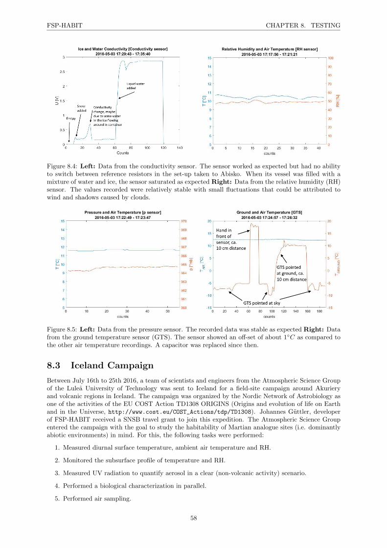
FSP-HABIT CHAPTER 8. TESTING
Figure 8.4: Left: Data from the conductivity sensor. The sensor worked as expected but had no abilityto switch between reference resistors in the set-up taken to Abisko. When its vessel was filled with amixture of water and ice, the sensor saturated as expected Right: Data from the relative humidity (RH)sensor. The values recorded were relatively stable with small fluctuations that could be attributed towind and shadows caused by clouds.
Figure 8.5: Left: Data from the pressure sensor. The recorded data was stable as expected Right: Datafrom the ground temperature sensor (GTS). The sensor showed an off-set of about 1C as compared tothe other air temperature recordings. A capacitor was replaced since then.
8.3 Iceland Campaign
Between July 16th to 25th 2016, a team of scientists and engineers from the Atmospheric Science Groupof the Lulea University of Technology was sent to Iceland for a field-site campaign around Akurieryand volcanic regions in Iceland. The campaign was organized by the Nordic Network of Astrobiology asone of the activities of the EU COST Action TD1308 ORIGINS (Origins and evolution of life on Earthand in the Universe, http://www.cost.eu/COST_Actions/tdp/TD1308). Johannes Guttler, developerof FSP-HABIT received a SNSB travel grant to join this expedition. The Atmospheric Science Groupentered the campaign with the goal to study the habitability of Martian analogue sites (i.e. dominantlyabiotic environments) in mind. For this, the following tasks were performed:
1. Measured diurnal surface temperature, ambient air temperature and RH.
2. Monitored the subsurface profile of temperature and RH.
3. Measured UV radiation to quantify aerosol in a clear (non-volcanic activity) scenario.
4. Performed a biological characterization in parallel.
5. Performed air sampling.
58

FSP-HABIT CHAPTER 8. TESTING
6. Tested a HABIT prototype (FSP-HABIT).
The goals have been realized by taking soil, ice, water and air samples as well as by taking measure-ments with scientific instrumentation. The instruments taken to Iceland for this were the FSP-HABIT(Field-Site Prototype for HABIT), a PeakTech 5040 3-in-1 IR temperature and relative humidity meter,a ThermoFisher Orion Star A329 pH/ISE/conductivity meter, and a HOBO H21 weather station withUV sensors. Having a wide array of instruments was beneficial for comparing the measurements doneby FSP-HABIT to the data from the other instruments.
The geomorphological features of Tungnafellsjokull glacier, specifically the way they are changing tem-porally with respect to the volcanic activities at Bardabunga were analyzed. Additionally, the affectof volcanic activities on overall glacier dynamics were studied and a comparative study of its dynamicswith respect to the Himalayan glaciers was prepared by members of the Atmospheric Science Group.For this, field photographs of geomorphology were taken. With an elevation of 1,535 meters, this glacieris relatively small and well suited for an assessment. It was also the nearest Icelandic glacier from bothAkureyri and Bardabunga (about 20 km away).
The biological colonization of fresh lava fields such as Leirhunkur has been studied with samples currentlybeing analyzed. Analyzed were fresh lava fields during and after cooling, before primary colonization andthen over time with colonization of the degassing and drying basalt. Many parts of the lava field werestill too hot to colonize, whilst other areas have cooled enough to allow initial microbial colonization.The team traveled to Martian analogue sites such as Gjastykki, to the Hverfjall explosion crater, theVikursandur sandy field and other areas as seen in figure 8.6.
Figure 8.6: Left: Areas traveled to in Iceland. Right: The HABIT prototype in a Martian analoguesite in Iceland
Iceland marked the first time a HABIT prototype was deployed during a field-site campaign. FSP-HABITcharacterized salts by their conductivity and its measurements were used to characterize the near surfaceenvironment. These measurements were then available for comparison with the microbiological studiesof the water, ices and soils to characterize the habitability of the explored site. The deployment ofthe prototype was an overall success, even though the robustness of it showed need for improvementfor future campaigns. The method of measuring the conductivity of brines at 3 different measurementheights was validated. Several design improvements such as a sturdier mount for the relative humiditysensor were taken note of. Unfortunately, the most of relevant salts were not available in Iceland andso the following salts were tested: Calcium chloride (CaCl2), potassium hydroxide (KOH), and sodiumhydroxide (NaOH), all obtained from the University of Akuriery. KOH and NaOH were chosen fortheir similarity with the perchlorates on Mars, namely their corrosive and hygroscopic nature. Nextfollows a discussion of the recorded data from the Iceland campaign.
The following data has been recorded on July 20 during a 3 h 19 min test-run next to the Vıti craterwithin the Krafla volcanic system in the Myvatn region. Figure 8.7 shows the voltages recorded for CaCl2
59

FSP-HABIT CHAPTER 8. TESTING
with 5 different reference resistors, ranging from 1 MΩ down to 100 Ω. Each vessels took measurementson three different measurement heights, indicated by V 21, V 22, and V 23 for salt vessel 2, top, middle,and bottom. The salt was made from fine grains. All measurements have in common that they show aspike at the beginning of the test run which has likely been caused by the transportation from the car,where the salts were filled into the salt vessels and the measurements were started, to the measurementsite, several hundred meters away. This means that the conductivity measurements can be affected byvibrations on the prototype and/or displacement of the salts. The voltage recorded at height V 21 (top)remains zero for the full duration of the test run. This is consistent with the vessels being filled up tothe middle with CaCl2 and therefore no salt was between the electrodes at that height. V 22 (middle)showed the most interesting signal: For larger reference resistors, the sensor jumps to a saturation valueat about 155 minutes into the measurement. However, the voltage measured at the 100 Ω referenceresistor does only increase by a small amount. The 1 kΩ reference resistor is the only one to show afluctuating voltage. As explained in prior chapters, the conductivity sensors functions by performing avoltage division between the reference resistor and the resistance of the brine. If the resistance of thebrine is low compared to the reference resistor, most of the voltage will be found across the referenceresistor. This is the case for 10 kΩ, the 100 kΩ, and the 1 MΩ resistors. At the same time, if theresistance of the brine is high as compared to the reference resistance, then all of the voltage would falloff on the brine, thus the voltage recorded is low. This is the case for the 100 Ω resistor (and for an openloop between the electrodes). The fluctuating signal at the 1 kΩ resistor indicates that the resistance ofthe brine was of the same magnitude as the reference resistor. The sudden appearance of the signal atabout 155 minutes is conceivable as droplets of water can suddenly combine when they reached a greatenough size. What could have happened is that a drop of water moved onto the electrode at 155 minutesand thus closed the electrical circuit so that a signal was detectable. This theory is strengthened by theobserved liquid film on top of the salt during later disassembly at the end of the experiment. The signalrecorded by V 23 was less conclusive: Reference resistors 100 kΩ through to 100 Ω did not record anysignal while the 1 MΩ did show a saturated signal at the 155 minutes mark, just like the V 22 signal.However, the measurements for KOH and NaOH at the 1 MΩ reference resistors also differ from themeasurements with the other reference resistors. This is the case for the KOH V 42 measurements andthe NaOH V 62 measurements. This could indicate a systematic issue with the 1 MΩ reference resistor.
0 20 40 60 80 100 120 140 160 180 200
t [min]
024
U [
V]
Conductivity CaCl2
1MOhm Reference ResistorV2
1
V22
V23
0 20 40 60 80 100 120 140 160 180 200
t [min]
024
U [
V]
Conductivity CaCl2
100k Reference ResistorV2
1
V22
V23
0 20 40 60 80 100 120 140 160 180 200
t [min]
024
U [
V]
Conductivity CaCl2
10k Reference ResistorV2
1
V22
V23
0 20 40 60 80 100 120 140 160 180 200
t [min]
0
0.5
1
U [
V]
Conductivity CaCl2
1k Reference ResistorV2
1
V22
V23
0 20 40 60 80 100 120 140 160 180 200
t [min]
00.5
1
U [
V]
Conductivity CaCl2
100 Reference ResistorV2
1
V22
V23
Figure 8.7: CaCl2 conductivity values for all used reference resistors from the Vıti field-site.
Next, the conductivity recordings for potassium hydroxide (KOH) are discussed. The salt came in theform of pellets. Because of their form factor, the pellets were located at all measurement heights. Animage of all vessels shortly after being filled with the three salts is shown in figure 8.12 at the end ofthis chapter. As can be seen in figure 8.8, the measurement points V 41 and V 43 show early saturationfor the larger reference resistors (1 MΩ, 100 kΩ) and a steady signal increase for the smaller resistors (1kΩ, 100 Ω). The signal at the 10 kΩ reference resistors is found in between the larger and the smallerresistors and steadily increases within the first 40 minutes of the experiment were it reaches a steady
60
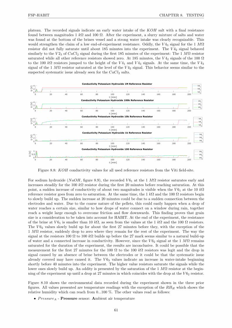
FSP-HABIT CHAPTER 8. TESTING
plateau. The recorded signals indicate an early water intake of the KOH salt with a final resistancefound between magnitudes 1 kΩ and 100 Ω. After the experiment, a slurry mixture of salts and waterwas found at the bottom of the brines vessel and a strong water intake was clearly recognizable. Thiswould strengthen the claim of a low end-of-experiment resistance. Oddly, the V 43 signal for the 1 MΩresistor did not fully saturate until about 185 minutes into the experiment. The V 42 signal behavedsimilarly to the V 23 of CaCl2 signal during the first 185 minutes of the experiment: The 1 MΩ resistorsaturated while all other reference resistors showed zero. At 185 minutes, the V 42 signals of the 100 Ωto the 100 kΩ resistors jumped to the height of the V 41 and V 43 signals. At the same time, the V 43signal of the 1 MΩ resistor saturated at the level of the V 42 signal. This behavior seems similar to thesuspected systematic issue already seen for the CaCl2 salts.
0 20 40 60 80 100 120 140 160 180 200
t [min]
0
2
4
U [
V]
Conductivity Potassium Hydroxide 1M Reference ResistorV4
1
V42
V43
0 20 40 60 80 100 120 140 160 180 200
t [min]
0
2
4
U [
V]
Conductivity Potassium Hydroxide 100k Reference Resistor V41
V42
V43
0 20 40 60 80 100 120 140 160 180 200
t [min]
0
2
4
U [
V]
Conductivity Potassium Hydroxide 10k Reference ResistorV4
1
V42
V43
0 20 40 60 80 100 120 140 160 180 200
t [min]
0
2
4
U [
V]
Conductivity Potassium Hydroxide 1k Reference ResistorV4
1
V42
V43
0 20 40 60 80 100 120 140 160 180 200
t [min]
0
0.5
1
U [
V]
Conductivity Potassium Hydroxide 100 Reference ResistorV4
1
V42
V43
Figure 8.8: KOH conductivity values for all used reference resistors from the Vıti field-site.
For sodium hydroxide (NaOH, figure 8.9), the recorded V 61 at the 1 MΩ resistor saturates early andincreases steadily for the 100 kΩ resistor during the first 20 minutes before reaching saturation. At thispoint, a sudden increase of conductivity of about two magnitudes is visible when the V 61 at the 10 kΩreference resistor goes from zero to saturation. At the same time, the 1 kΩ and the 100 Ω resistors beginto slowly build up. The sudden increase at 20 minutes could be due to a sudden connection between theelectrodes and water. Due to the coarse nature of the pellets, this could easily happen when a drop ofwater reaches a certain size, similar to how drops of water connect on a window during rain, togetherreach a weight large enough to overcome friction and flow downwards. This finding proves that grainsize is a consideration to be taken into account for HABIT. At the end of the experiment, the resistanceof the brine at V 61 is smaller than 10 kΩ, as seen from the values at the 1 kΩ and the 100 Ω resistors.The V 62 values slowly build up for about the first 27 minutes before they, with the exception of the1 MΩ resistor, suddenly drop to zero where they remain for the rest of the experiment. The way thesignal at the resistors 100 Ω to 100 kΩ builds up before the 27 mark seems similar to a natural build-upof water and a connected increase in conductivity. However, since the V 62 signal at the 1 MΩ remainssaturated for the duration of the experiment, the results are inconclusive. It could be possible that themeasurement for the first 27 minutes for the 100 Ω to the 100 kΩ resistors was legit and the drop insignal caused by an absence of brine between the electrodes or it could be that the systematic issuealready covered may have caused it. The V 63 values indicate an increase in water-intake beginningshortly before 40 minutes into the experiment. The higher value resistors saturate the signals while thelower ones slowly build up. An oddity is presented by the saturation of the 1 MΩ resistor at the begin-ning of the experiment up until a drop at 27 minutes in which coincides with the drop at the V 62 resistor.
Figure 8.10 shows the environmental data recorded during the experiment shown in the three priorfigures. All values presented are temperature readings with the exception of the RHH which shows therelative humidity which can reach from 0...100 %. The other values read as follows:
PressureA - Pressure sensor: Ambient air temperature
61

FSP-HABIT CHAPTER 8. TESTING
0 20 40 60 80 100 120 140 160 180 200
t [min]
0
2
4U
[V]
Conductivity Sodium Hydroxide 1M Reference Resistor
V61
V62
V63
0 20 40 60 80 100 120 140 160 180 200
t [min]
0
2
4
U [
V]
Conductivity Sodium Hydroxide 100k Reference Resistor
V61
V62
V63
0 20 40 60 80 100 120 140 160 180 200
t [min]
0
2
4
U [
V]
Conductivity Sodium Hydroxide 10k Reference Resistor V61
V62
V63
0 20 40 60 80 100 120 140 160 180 200
t [min]
0
2
4
U [
V]
Conductivity Sodium Hydroxide 1k Reference Resistor
V61
V62
V63
0 20 40 60 80 100 120 140 160 180 200
t [min]
0
1
2
U [
V]
Conductivity Sodium Hydroxide 100 Reference Resistor
V61
V62
V63
Figure 8.9: NaOH conductivity values for all used reference resistors from the Vıti field-site.
GTSA - Ground Temperature Sensor: Ambient air temperature
GTSG - Ground Temperature Sensor: Ground temperature recorded by the IR-sensor
RHA - Relative Humidity sensor: Ambient air temperature
0 20 40 60 80 100 120 140 160 180 200
t [min]
10
20
30
40
50
60
70
80
T [
°C];
RH
[%
]
ICELAND 160720 1623-1942 G1
PressureA
GTSA
GTSG
RHA
RHH
Figure 8.10: Temperature and RH data recorded by FSP-HABIT’s ENVPACK at the Vıti field-site.
Data was recorded between 16:23 to 19:42 local time on a cloudy day with intermittent openings whichallowed the Sun to shine through. The ambient temperature recorded by the pressure sensor is visiblyhigher than the other temperatures seen in the graph, reaching values higher than 30C about between80 to 100 minutes into the experiment. This can be explained by the orientation of the instrument: TheFSP-HABIT was oriented so that its back was pointing towards the Sun while the two other sensors(GTS, RHS) were in the shadow of the instrument. The anti-correlation of the air temperature with theRH is clearly visible, especially around the 100 minutes mark when the temperature drops several degreesand the relative humidity rises by more than 10 percent. Notable is an increase in the air temperature
62

FSP-HABIT CHAPTER 8. TESTING
prior to the drop, beginning about 40 minutes into the measurements. The rise is most pronounced forthe temperature recordings of the pressure sensor. Since the temperatures are continuously lower afterthe drop at 100 minutes, it can be assumed that the prototype was subjected to the Sun from 40...100min and then in the clouds’ shadows. The heating by the Sun could have masked the general decrease inair temperature over time. The ground temperature value recorded by the GTS was found to be similarto the air temperatures.
The atmospheric pressure remained stable over the duration of the experiment, ranging from 942 hPa to944 hPa. Figure 8.11 shows the evolution of the atmospheric pressure for the conductivity measurementsintroduced prior. Figure 8.12 then shows the brines container assembly during filling of the salts andafter the experiment.
0 20 40 60 80 100 120 140 160 180 200
t [min]
938
939
940
941
942
943
944
945
p [
hPa
]
Pressure 160720 1623-1942 G1
Figure 8.11: Pressure data recorded by FSP-HABIT’s ENVPACK at the Vıti field-site.
Figure 8.12: The Brinces Container Assembly shortly after being filled with salts (top left), after 3:19 hof conductivity measurements (right), and close-ups of the three salts CaCl2, KOH, NaOH after theconductivity measurements (bottom left).
63

FSP-HABIT CHAPTER 8. TESTING
8.4 India Campaign
Between August 9th to 19th 2016, a team of scientists and engineers from the Atmospheric ScienceGroup of the Lulea University of Technology was sent to India for a field-site campaign in Ladakh,Himalaya. The campaign was organized by NASA’s Spaceward Bound (SB) program. Within the Space-ward Bound program, astrobiologists and astrogeoscientists conduct field experiments in various partsof the world. Particular interest is paid to areas which offer ’harsh or extreme environments and ex-hibit sustenance of life in the forms of singular or complex microorganisms’ (from the official websitehttp://spacewardbound.astrobiologyindia.in/). The program further is concerned with the originand evolution of topographic changes due to physical and chemical processes over time and the conditionsfor life to exist. This knowledge is then adapted to study challenges for life on Earth and in other ’hab-itable’ environments in the universe. Similar to the Iceland campaign, the Atmospheric Science Groupentered the campaign with the goal to study the habitability of Martian analogue sites (i.e. dominantlyabiotic environments) in mind. For this, the same steps as described in the chapter covering the Icelandcampaign were performed (chapter 8.3). Again, the commercial instruments that have been introducedin the Iceland chapter were with the scientists to allow for comparison. Ladakh was chosen by the SBorganizers for its unique combination of extreme temperatures due to the arid cold dessert environment,hot springs, saline lakes, glaciers, high UV doses, the occurrence of permafrost and altitudes above 3000meters (no vegetation). Further, the low population of the region offers pristine conditions to conductexperiments. While most of the above stated parameters were actually found at the visited field-sites,FSP-HABIT also experienced high temperatures, heating the prototype up to 54C, as will be shownmomentarily. The expedition included teams covering the five different research areas, ranging frommicrobiology and geology to paleo-botany, robotics and atmospheric science.
Between the Iceland and the India campaign, two days were available to fix an issue with the conductivitysensor. During the Iceland campaign, the prototype was subjected to a wide array of different stresses,ranging from differences in temperatures and humidities to hours of vibrations during hour-long driveson rocky roads to dropping down a muddy hill. During the fixing period, it was discovered that theARDUINO could not provide the required voltage at its digital input/outputs for the analog switchesanymore. A set of pull up resistors was put in place in order to cope with this issue. Figure 7.4 showsthe newly added components in the ARDUINO compartment.
In the following, the data recorded during the India campaign will be shown. The data is presented assets of two vessels each since there were always two vessels filled with the same salt, i.e. vessels 1 and 2were filled with sodium perchlorate, vessels 3 and 4 were filled with calcium perchlorate, and vessels 5and 6 were filled with calcium chloride. This was done to see differences in the signal recorded for thesame salt. In the case of vessel 5 and 6 it further gives some insight in the differences between locatingthe salts under a lid as compared to having them in direct contact with the atmosphere since vessel 6 isthe reference vessel and open on top. All sets are structured so that the left side of the figures representsone vessel while the right side of the figures represent the other vessel. This is done for five referenceresistors per vessel, beginning with the largest resistor, 1 MΩ, and then going down to the lowest resistorthrough the 100 kΩ, 10 kΩ, 1 kΩ, down to the 100 Ω reference resistor. The results shown are givenin volts. This gives an immediate overview of the behavior of the instrument and an estimate of thehydration state of the salts. The last row is not specific to the vessels but contains data recorded byENVPACK, namely the relative humidity recorded by the RHS and the temperatures recorded by theRHS, GTS, and PS which have been plotted on the same time scale. These parameters are also foundplotted separately in appendix A.
64
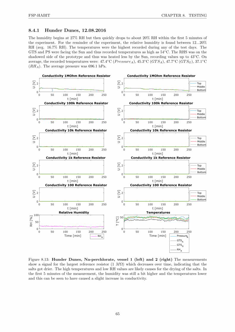
FSP-HABIT CHAPTER 8. TESTING
8.4.1 Hunder Dunes, 12.08.2016
The humidity begins at 27% RH but then quickly drops to about 20% RH within the first 5 minutes ofthe experiment. For the reminder of the experiment, the relative humidity is found between 12...20%RH (avg. 16.7% RH). The temperatures were the highest recorded during any of the test days. TheGTS and PS were facing the Sun and thus recorded temperatures as high as 54C. The RHS was on theshadowed side of the prototype and thus was heated less by the Sun, recording values up to 43C. Onaverage, the recorded temperatures were: 47.4C (PressureA), 45.3C (GTSA), 47.7C (GTSG), 37.1C(RHA). The average pressure was 696.1 hPa.
0 50 100 150 200 250
t [min]
0
2
U [
V]
Conductivity 1MOhm Reference Resistor
0 50 100 150 200 250
t [min]
0
2
U [
V]
Conductivity 100k Reference Resistor
0 50 100 150 200 250
t [min]
0
2
U [
V]
Conductivity 10k Reference Resistor
0 50 100 150 200 250
t [min]
0
2
U [
V]
Conductivity 1k Reference Resistor
0 50 100 150 200 250
t [min]
0
2
U [
V]
Conductivity 100 Reference Resistor
0 50 100 150 200 250
Time [min]
0
50
100
RH
[%
]
Relative Humidity
RHH
0 50 100 150 200 250
t [min]
0
2
U [
V]
Conductivity 1MOhm Reference Resistor
TopMiddleBottom
0 50 100 150 200 250
t [min]
0
2
U [
V]
Conductivity 100k Reference Resistor
TopMiddleBottom
0 50 100 150 200 250
t [min]
0
2
U [
V]
Conductivity 10k Reference Resistor
TopMiddleBottom
0 50 100 150 200 250
t [min]
0
2
U [
V]
Conductivity 1k Reference Resistor
TopMiddleBottom
0 50 100 150 200 250
t [min]
0
2
U [
V]
Conductivity 100 Reference Resistor
TopMiddleBottom
0 50 100 150 200 250
Time [min]
0
50
T [
°C]
Temperatures
PressureAGTSA
GTSG
RHA
Figure 8.13: Hunder Dunes, Na-perchlorate, vessel 1 (left) and 2 (right) The measurementsshow a signal for the largest reference resistor (1 MΩ) which decreases over time, indicating that thesalts got drier. The high temperatures and low RH values are likely causes for the drying of the salts. Inthe first 5 minutes of the measurement, the humidity was still a bit higher and the temperatures lowerand this can be seen to have caused a slight increase in conductivity.
65
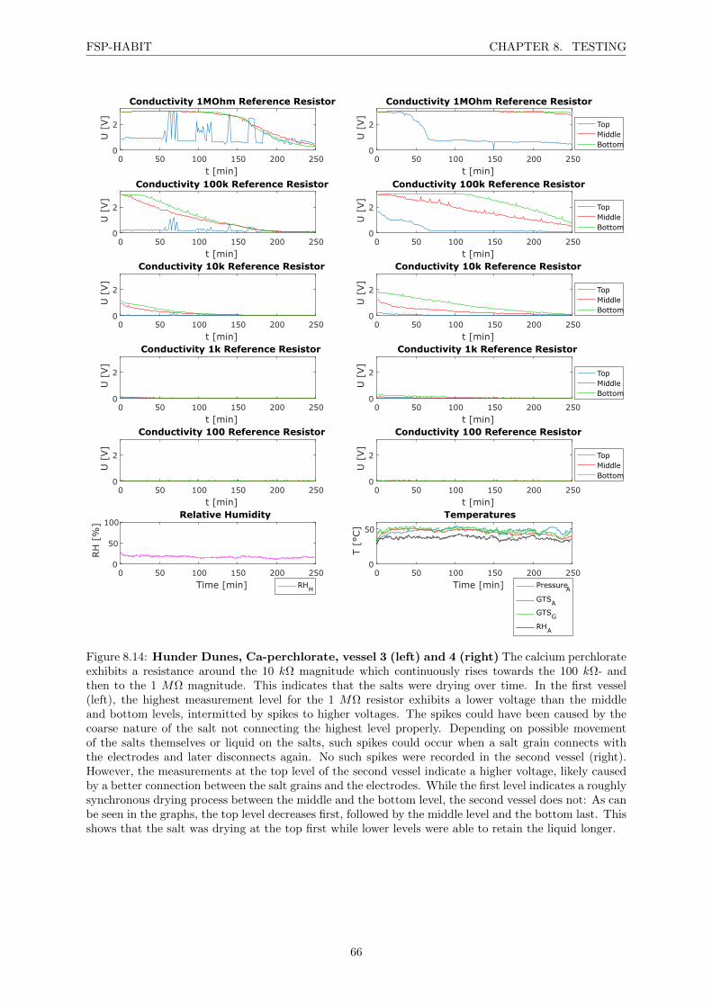
FSP-HABIT CHAPTER 8. TESTING
0 50 100 150 200 250
t [min]
0
2
U [
V]
Conductivity 1MOhm Reference Resistor
0 50 100 150 200 250
t [min]
0
2
U [
V]
Conductivity 100k Reference Resistor
0 50 100 150 200 250
t [min]
0
2
U [
V]
Conductivity 10k Reference Resistor
0 50 100 150 200 250
t [min]
0
2
U [
V]
Conductivity 1k Reference Resistor
0 50 100 150 200 250
t [min]
0
2
U [
V]
Conductivity 100 Reference Resistor
0 50 100 150 200 250
Time [min]
0
50
100
RH
[%
]
Relative Humidity
RHH
0 50 100 150 200 250
t [min]
0
2
U [
V]
Conductivity 1MOhm Reference Resistor
TopMiddleBottom
0 50 100 150 200 250
t [min]
0
2
U [
V]
Conductivity 100k Reference Resistor
TopMiddleBottom
0 50 100 150 200 250
t [min]
0
2
U [
V]
Conductivity 10k Reference Resistor
TopMiddleBottom
0 50 100 150 200 250
t [min]
0
2
U [
V]
Conductivity 1k Reference Resistor
TopMiddleBottom
0 50 100 150 200 250
t [min]
0
2
U [
V]
Conductivity 100 Reference Resistor
TopMiddleBottom
0 50 100 150 200 250
Time [min]
0
50
T [
°C]
Temperatures
PressureAGTSA
GTSG
RHA
Figure 8.14: Hunder Dunes, Ca-perchlorate, vessel 3 (left) and 4 (right) The calcium perchlorateexhibits a resistance around the 10 kΩ magnitude which continuously rises towards the 100 kΩ- andthen to the 1 MΩ magnitude. This indicates that the salts were drying over time. In the first vessel(left), the highest measurement level for the 1 MΩ resistor exhibits a lower voltage than the middleand bottom levels, intermitted by spikes to higher voltages. The spikes could have been caused by thecoarse nature of the salt not connecting the highest level properly. Depending on possible movementof the salts themselves or liquid on the salts, such spikes could occur when a salt grain connects withthe electrodes and later disconnects again. No such spikes were recorded in the second vessel (right).However, the measurements at the top level of the second vessel indicate a higher voltage, likely causedby a better connection between the salt grains and the electrodes. While the first level indicates a roughlysynchronous drying process between the middle and the bottom level, the second vessel does not: As canbe seen in the graphs, the top level decreases first, followed by the middle level and the bottom last. Thisshows that the salt was drying at the top first while lower levels were able to retain the liquid longer.
66
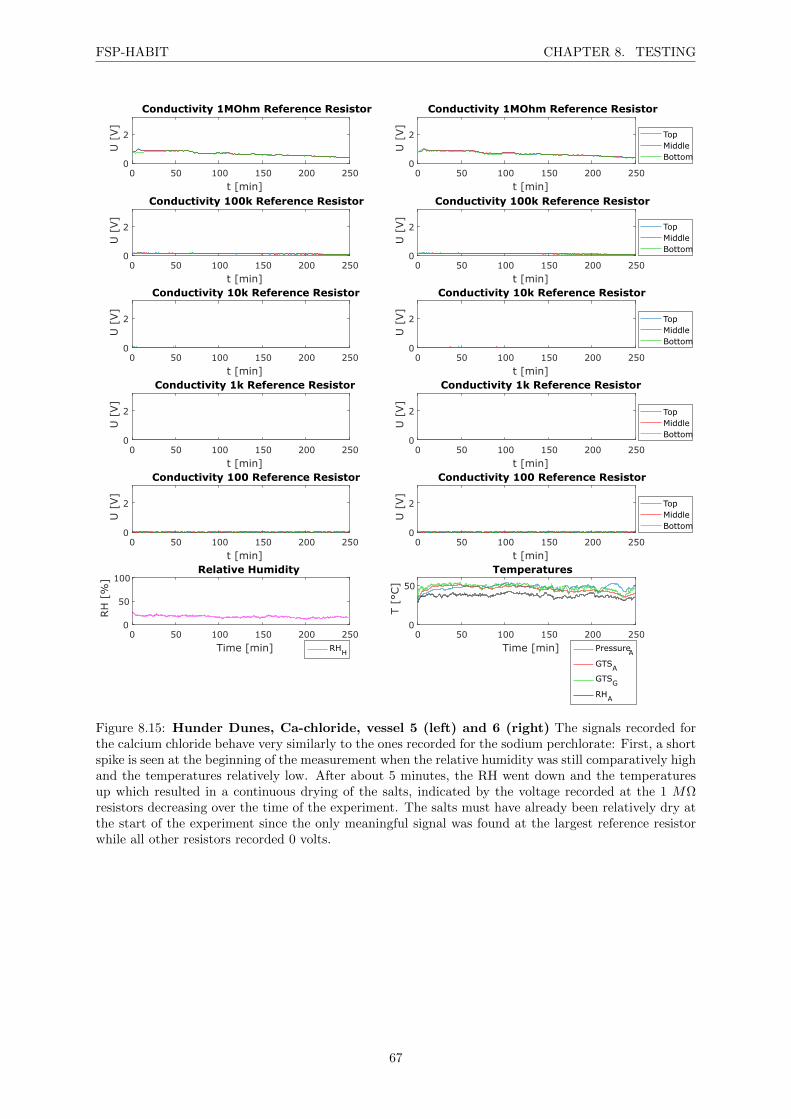
FSP-HABIT CHAPTER 8. TESTING
0 50 100 150 200 250
t [min]
0
2
U [
V]
Conductivity 1MOhm Reference Resistor
0 50 100 150 200 250
t [min]
0
2
U [
V]
Conductivity 100k Reference Resistor
0 50 100 150 200 250
t [min]
0
2
U [
V]
Conductivity 10k Reference Resistor
0 50 100 150 200 250
t [min]
0
2
U [
V]
Conductivity 1k Reference Resistor
0 50 100 150 200 250
t [min]
0
2
U [
V]
Conductivity 100 Reference Resistor
0 50 100 150 200 250
Time [min]
0
50
100
RH
[%
]
Relative Humidity
RHH
0 50 100 150 200 250
t [min]
0
2
U [
V]
Conductivity 1MOhm Reference Resistor
TopMiddleBottom
0 50 100 150 200 250
t [min]
0
2
U [
V]
Conductivity 100k Reference Resistor
TopMiddleBottom
0 50 100 150 200 250
t [min]
0
2
U [
V]
Conductivity 10k Reference Resistor
TopMiddleBottom
0 50 100 150 200 250
t [min]
0
2U
[V]
Conductivity 1k Reference Resistor
TopMiddleBottom
0 50 100 150 200 250
t [min]
0
2
U [
V]
Conductivity 100 Reference Resistor
TopMiddleBottom
0 50 100 150 200 250
Time [min]
0
50
T [
°C]
Temperatures
PressureAGTSA
GTSG
RHA
Figure 8.15: Hunder Dunes, Ca-chloride, vessel 5 (left) and 6 (right) The signals recorded forthe calcium chloride behave very similarly to the ones recorded for the sodium perchlorate: First, a shortspike is seen at the beginning of the measurement when the relative humidity was still comparatively highand the temperatures relatively low. After about 5 minutes, the RH went down and the temperaturesup which resulted in a continuous drying of the salts, indicated by the voltage recorded at the 1 MΩresistors decreasing over the time of the experiment. The salts must have already been relatively dry atthe start of the experiment since the only meaningful signal was found at the largest reference resistorwhile all other resistors recorded 0 volts.
67

FSP-HABIT CHAPTER 8. TESTING
8.4.2 Kardung La, 13.08.2016
This set of measurements was affected by the loose contact of the RHS. This can be seen in the relativehumidity being found at 0.10% between minute 0...7, 8...10, and for the last minute of the experiment.At the same times, the temperature recorded by the RHS has been found to be a constant 615.25C. Thetransitions between these values (0.10% RH, 615.25C) and more reasonable values are evident by sharpdrops in the case of the RH and sharp spikes in the case of the temperature. Values for the humidity arefound at around 42% RH between minute 11...22 and around 27% RH between minute 23 until the endof the experiment at minute 42. The average RH recorded was 34.2%. The prototype was shone ontoby the Sun from the top. On average, the recorded temperatures were: 19.0C (PressureA), 16.5C(GTSA), 15.4C (GTSG), 13.6C (RHA). The average pressure was 541.9 hPa.
0 10 20 30 40 50
t [min]
0
2
U [
V]
Conductivity 1MOhm Reference Resistor
0 10 20 30 40 50
t [min]
0
2
U [
V]
Conductivity 100k Reference Resistor
0 10 20 30 40 50
t [min]
0
2
U [
V]
Conductivity 10k Reference Resistor
0 10 20 30 40 50
t [min]
0
2
U [
V]
Conductivity 1k Reference Resistor
0 10 20 30 40 50
t [min]
0
2
U [
V]
Conductivity 100 Reference Resistor
0 10 20 30 40 50
Time [min]
0
50
100
RH
[%
]
Relative Humidity
RHH
0 10 20 30 40 50
t [min]
0
2
U [
V]
Conductivity 1MOhm Reference Resistor
TopMiddleBottom
0 10 20 30 40 50
t [min]
0
2U
[V]
Conductivity 100k Reference Resistor
TopMiddleBottom
0 10 20 30 40 50
t [min]
0
2
U [
V]
Conductivity 10k Reference Resistor
TopMiddleBottom
0 10 20 30 40 50
t [min]
0
2
U [
V]
Conductivity 1k Reference Resistor
TopMiddleBottom
0 10 20 30 40 50
t [min]
0
2
U [
V]
Conductivity 100 Reference Resistor
TopMiddleBottom
0 10 20 30 40 50
Time [min]
0
50
T [
°C]
Temperatures
PressureAGTSA
GTSG
RHA
Figure 8.16: Kardung La, Na-perchlorate, vessel 1 (left) and 2 (right) The most distinct featureof this set of measurements is the lack of notable change over the duration of the experiment. Thisindicates a lack of water intake by or a drying of the salts. The most distinct feature is seen for vessel 1(left) at the 1 MΩ reference resistor showing a drop between minute 30...32.5 that might be an error inthe measurements. This is suspected as the drop is caused by a single outlier which is not visible at the100 kΩ resistor (the values measured at the different resistors usually follow each other).
68

FSP-HABIT CHAPTER 8. TESTING
0 10 20 30 40 50
t [min]
0
2
U [
V]
Conductivity 1MOhm Reference Resistor
0 10 20 30 40 50
t [min]
0
2
U [
V]
Conductivity 100k Reference Resistor
0 10 20 30 40 50
t [min]
0
2
U [
V]
Conductivity 10k Reference Resistor
0 10 20 30 40 50
t [min]
0
2
U [
V]
Conductivity 1k Reference Resistor
0 10 20 30 40 50
t [min]
0
2
U [
V]
Conductivity 100 Reference Resistor
0 10 20 30 40 50
Time [min]
0
50
100
RH
[%
]
Relative Humidity
RHH
0 10 20 30 40 50
t [min]
0
2
U [
V]
Conductivity 1MOhm Reference Resistor
TopMiddleBottom
0 10 20 30 40 50
t [min]
0
2
U [
V]
Conductivity 100k Reference Resistor
TopMiddleBottom
0 10 20 30 40 50
t [min]
0
2
U [
V]
Conductivity 10k Reference Resistor
TopMiddleBottom
0 10 20 30 40 50
t [min]
0
2U
[V]
Conductivity 1k Reference Resistor
TopMiddleBottom
0 10 20 30 40 50
t [min]
0
2
U [
V]
Conductivity 100 Reference Resistor
TopMiddleBottom
0 10 20 30 40 50
Time [min]
0
50
T [
°C]
Temperatures
PressureAGTSA
GTSG
RHA
Figure 8.17: Kardung La, Ca-perchlorate, vessel 3 (left) and 4 (right) Similar to the valuesrecorded for the sodium perchlorate, the measurements for the calcium perchlorate do not show muchvariation over the time of the experiment. However, distinct differences between the measurement heightstop, middle, and bottom are distinguishable. In the third vessel(left) the voltage recorded at the toplevel is lower than at the middle and bottom ones. This can be seen at the values for the 1 MΩ, 100kΩ and at the 10 kΩ reference resistors while the other two resistors do not exhibit a distinct signal. Aslight rise in voltage, and therefore conductivity, is visible at the middle and bottom level measurementsfor the 100 kΩ resistor within the first 10 minutes of the experiment. Between 20 minutes until the endof the experiment, the conductivity at the same reference resistor reduces again slightly, possibly linkedto the reduction in relative humidity recorded during the same time. In vessel 4 (right), the voltage atthe 100 kΩ and 10 kΩ reference resistors show the highest conductivity at the bottom level, followed bythe top and by the middle level.
69

FSP-HABIT CHAPTER 8. TESTING
0 10 20 30 40 50
t [min]
0
2
U [
V]
Conductivity 1MOhm Reference Resistor
0 10 20 30 40 50
t [min]
0
2
U [
V]
Conductivity 100k Reference Resistor
0 10 20 30 40 50
t [min]
0
2
U [
V]
Conductivity 10k Reference Resistor
0 10 20 30 40 50
t [min]
0
2
U [
V]
Conductivity 1k Reference Resistor
0 10 20 30 40 50
t [min]
0
2
U [
V]
Conductivity 100 Reference Resistor
0 10 20 30 40 50
Time [min]
0
50
100
RH
[%
]
Relative Humidity
RHH
0 10 20 30 40 50
t [min]
0
2
U [
V]
Conductivity 1MOhm Reference Resistor
TopMiddleBottom
0 10 20 30 40 50
t [min]
0
2
U [
V]
Conductivity 100k Reference Resistor
TopMiddleBottom
0 10 20 30 40 50
t [min]
0
2
U [
V]
Conductivity 10k Reference Resistor
TopMiddleBottom
0 10 20 30 40 50
t [min]
0
2U
[V]
Conductivity 1k Reference Resistor
TopMiddleBottom
0 10 20 30 40 50
t [min]
0
2
U [
V]
Conductivity 100 Reference Resistor
TopMiddleBottom
0 10 20 30 40 50
Time [min]
0
50
T [
°C]
Temperatures
PressureAGTSA
GTSG
RHA
Figure 8.18: Kardung La, Ca-chloride, vessel 5 (left) and 6 (right) This set of measurementsexhibits an interesting difference between the two vessels: While the fifth vessel (left) shows rather strongsignals in the 1 MΩ, 100 kΩ, and 10 kΩ resistors, the sixth vessel (right) shows only moderate voltagelevels in the largest reference resistor. This could hint at differences between the salts’ behavior whenunder the BCA lid as compared to being directly exposed to the environment (like vessel 6). It is notablethat this was the only measurement were such large differences between two vessels of the same salt wererecorded. A reasonable assumption could have been to assume high wind speeds to carry away liquidfaster in the open vessel case (vessel 6, the reference vessel). However, the average wind speed recordedat Kardung La by the HOBO weather station was moderate with 2.58 m/s and nowhere near windspeeds recorded at Taglang La (avg. 8.33 m/s), where no such differences between the lid-covered vessel5 the open vessel 6 are visible. As described previously, the relative humidity was found at roughly42% RH prior to the 22 minute mark after which the RH drops to a lower level. The lid might havecreated an area above the salts which was able to hold the humidity for longer and thus enabled a risein conductivity through water intake. The moderate wind speed could have also played an enabling rolein this process as it allowed the air inside the lid to remain.
70
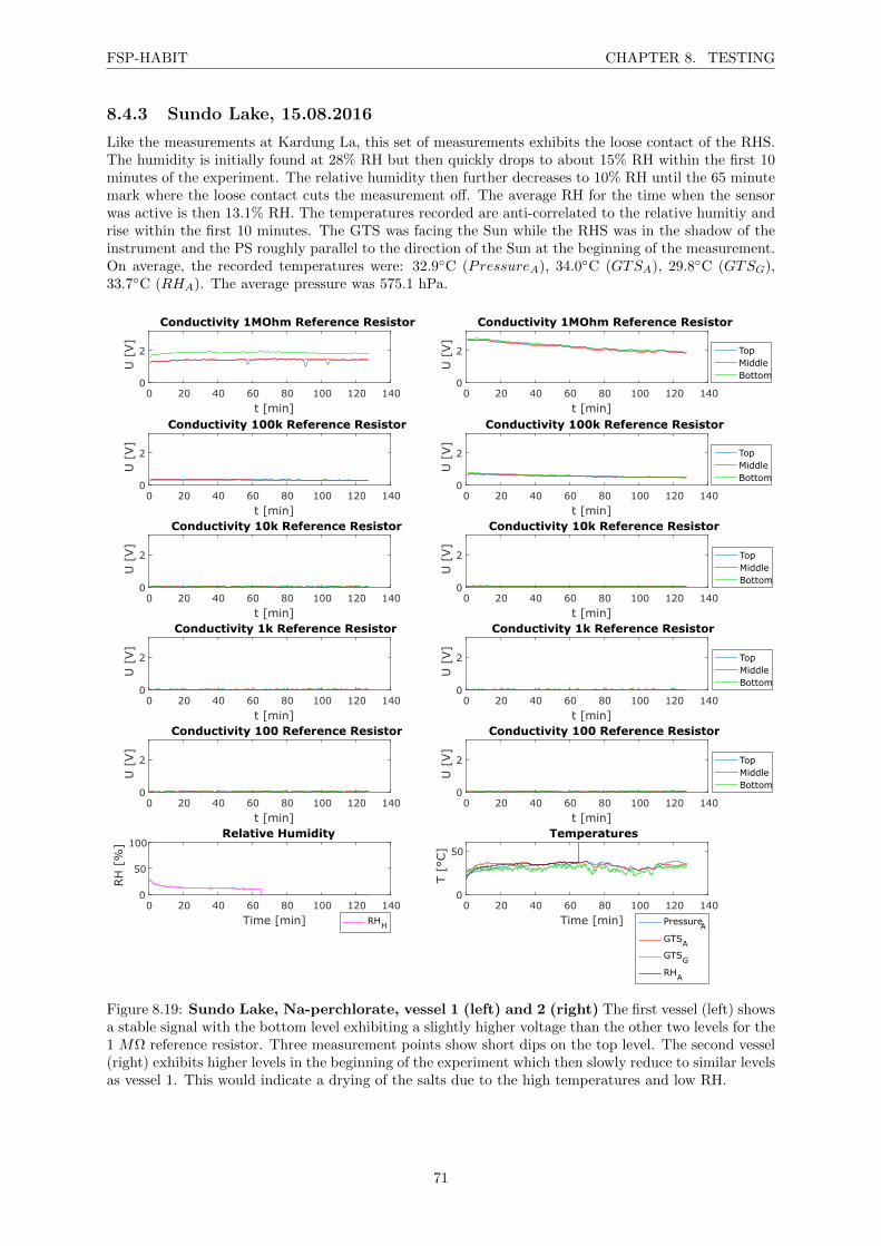
FSP-HABIT CHAPTER 8. TESTING
8.4.3 Sundo Lake, 15.08.2016
Like the measurements at Kardung La, this set of measurements exhibits the loose contact of the RHS.The humidity is initially found at 28% RH but then quickly drops to about 15% RH within the first 10minutes of the experiment. The relative humidity then further decreases to 10% RH until the 65 minutemark where the loose contact cuts the measurement off. The average RH for the time when the sensorwas active is then 13.1% RH. The temperatures recorded are anti-correlated to the relative humitiy andrise within the first 10 minutes. The GTS was facing the Sun while the RHS was in the shadow of theinstrument and the PS roughly parallel to the direction of the Sun at the beginning of the measurement.On average, the recorded temperatures were: 32.9C (PressureA), 34.0C (GTSA), 29.8C (GTSG),33.7C (RHA). The average pressure was 575.1 hPa.
0 20 40 60 80 100 120 140
t [min]
0
2
U [
V]
Conductivity 1MOhm Reference Resistor
0 20 40 60 80 100 120 140
t [min]
0
2
U [
V]
Conductivity 100k Reference Resistor
0 20 40 60 80 100 120 140
t [min]
0
2
U [
V]
Conductivity 10k Reference Resistor
0 20 40 60 80 100 120 140
t [min]
0
2
U [
V]
Conductivity 1k Reference Resistor
0 20 40 60 80 100 120 140
t [min]
0
2
U [
V]
Conductivity 100 Reference Resistor
0 20 40 60 80 100 120 140
Time [min]
0
50
100
RH
[%
]
Relative Humidity
RHH
0 20 40 60 80 100 120 140
t [min]
0
2
U [
V]
Conductivity 1MOhm Reference Resistor
TopMiddleBottom
0 20 40 60 80 100 120 140
t [min]
0
2U
[V]
Conductivity 100k Reference Resistor
TopMiddleBottom
0 20 40 60 80 100 120 140
t [min]
0
2
U [
V]
Conductivity 10k Reference Resistor
TopMiddleBottom
0 20 40 60 80 100 120 140
t [min]
0
2
U [
V]
Conductivity 1k Reference Resistor
TopMiddleBottom
0 20 40 60 80 100 120 140
t [min]
0
2
U [
V]
Conductivity 100 Reference Resistor
TopMiddleBottom
0 20 40 60 80 100 120 140
Time [min]
0
50
T [
°C]
Temperatures
PressureAGTSA
GTSG
RHA
Figure 8.19: Sundo Lake, Na-perchlorate, vessel 1 (left) and 2 (right) The first vessel (left) showsa stable signal with the bottom level exhibiting a slightly higher voltage than the other two levels for the1 MΩ reference resistor. Three measurement points show short dips on the top level. The second vessel(right) exhibits higher levels in the beginning of the experiment which then slowly reduce to similar levelsas vessel 1. This would indicate a drying of the salts due to the high temperatures and low RH.
71
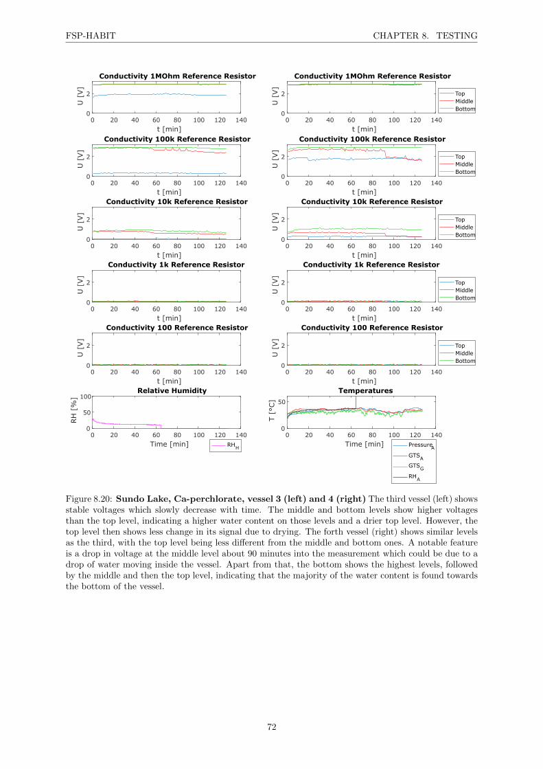
FSP-HABIT CHAPTER 8. TESTING
0 20 40 60 80 100 120 140
t [min]
0
2
U [
V]
Conductivity 1MOhm Reference Resistor
0 20 40 60 80 100 120 140
t [min]
0
2
U [
V]
Conductivity 100k Reference Resistor
0 20 40 60 80 100 120 140
t [min]
0
2
U [
V]
Conductivity 10k Reference Resistor
0 20 40 60 80 100 120 140
t [min]
0
2
U [
V]
Conductivity 1k Reference Resistor
0 20 40 60 80 100 120 140
t [min]
0
2
U [
V]
Conductivity 100 Reference Resistor
0 20 40 60 80 100 120 140
Time [min]
0
50
100
RH
[%
]
Relative Humidity
RHH
0 20 40 60 80 100 120 140
t [min]
0
2
U [
V]
Conductivity 1MOhm Reference Resistor
TopMiddleBottom
0 20 40 60 80 100 120 140
t [min]
0
2
U [
V]
Conductivity 100k Reference Resistor
TopMiddleBottom
0 20 40 60 80 100 120 140
t [min]
0
2
U [
V]
Conductivity 10k Reference Resistor
TopMiddleBottom
0 20 40 60 80 100 120 140
t [min]
0
2U
[V]
Conductivity 1k Reference Resistor
TopMiddleBottom
0 20 40 60 80 100 120 140
t [min]
0
2
U [
V]
Conductivity 100 Reference Resistor
TopMiddleBottom
0 20 40 60 80 100 120 140
Time [min]
0
50
T [
°C]
Temperatures
PressureAGTSA
GTSG
RHA
Figure 8.20: Sundo Lake, Ca-perchlorate, vessel 3 (left) and 4 (right) The third vessel (left) showsstable voltages which slowly decrease with time. The middle and bottom levels show higher voltagesthan the top level, indicating a higher water content on those levels and a drier top level. However, thetop level then shows less change in its signal due to drying. The forth vessel (right) shows similar levelsas the third, with the top level being less different from the middle and bottom ones. A notable featureis a drop in voltage at the middle level about 90 minutes into the measurement which could be due to adrop of water moving inside the vessel. Apart from that, the bottom shows the highest levels, followedby the middle and then the top level, indicating that the majority of the water content is found towardsthe bottom of the vessel.
72
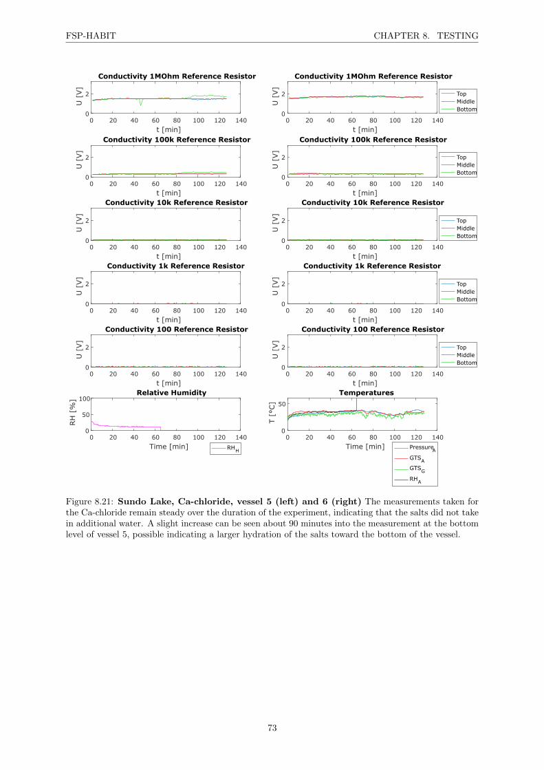
FSP-HABIT CHAPTER 8. TESTING
0 20 40 60 80 100 120 140
t [min]
0
2
U [
V]
Conductivity 1MOhm Reference Resistor
0 20 40 60 80 100 120 140
t [min]
0
2
U [
V]
Conductivity 100k Reference Resistor
0 20 40 60 80 100 120 140
t [min]
0
2
U [
V]
Conductivity 10k Reference Resistor
0 20 40 60 80 100 120 140
t [min]
0
2
U [
V]
Conductivity 1k Reference Resistor
0 20 40 60 80 100 120 140
t [min]
0
2
U [
V]
Conductivity 100 Reference Resistor
0 20 40 60 80 100 120 140
Time [min]
0
50
100
RH
[%
]
Relative Humidity
RHH
0 20 40 60 80 100 120 140
t [min]
0
2
U [
V]
Conductivity 1MOhm Reference Resistor
TopMiddleBottom
0 20 40 60 80 100 120 140
t [min]
0
2
U [
V]
Conductivity 100k Reference Resistor
TopMiddleBottom
0 20 40 60 80 100 120 140
t [min]
0
2
U [
V]
Conductivity 10k Reference Resistor
TopMiddleBottom
0 20 40 60 80 100 120 140
t [min]
0
2
U [
V]
Conductivity 1k Reference Resistor
TopMiddleBottom
0 20 40 60 80 100 120 140
t [min]
0
2
U [
V]
Conductivity 100 Reference Resistor
TopMiddleBottom
0 20 40 60 80 100 120 140
Time [min]
0
50
T [
°C]
Temperatures
PressureAGTSA
GTSG
RHA
Figure 8.21: Sundo Lake, Ca-chloride, vessel 5 (left) and 6 (right) The measurements taken forthe Ca-chloride remain steady over the duration of the experiment, indicating that the salts did not takein additional water. A slight increase can be seen about 90 minutes into the measurement at the bottomlevel of vessel 5, possible indicating a larger hydration of the salts toward the bottom of the vessel.
73
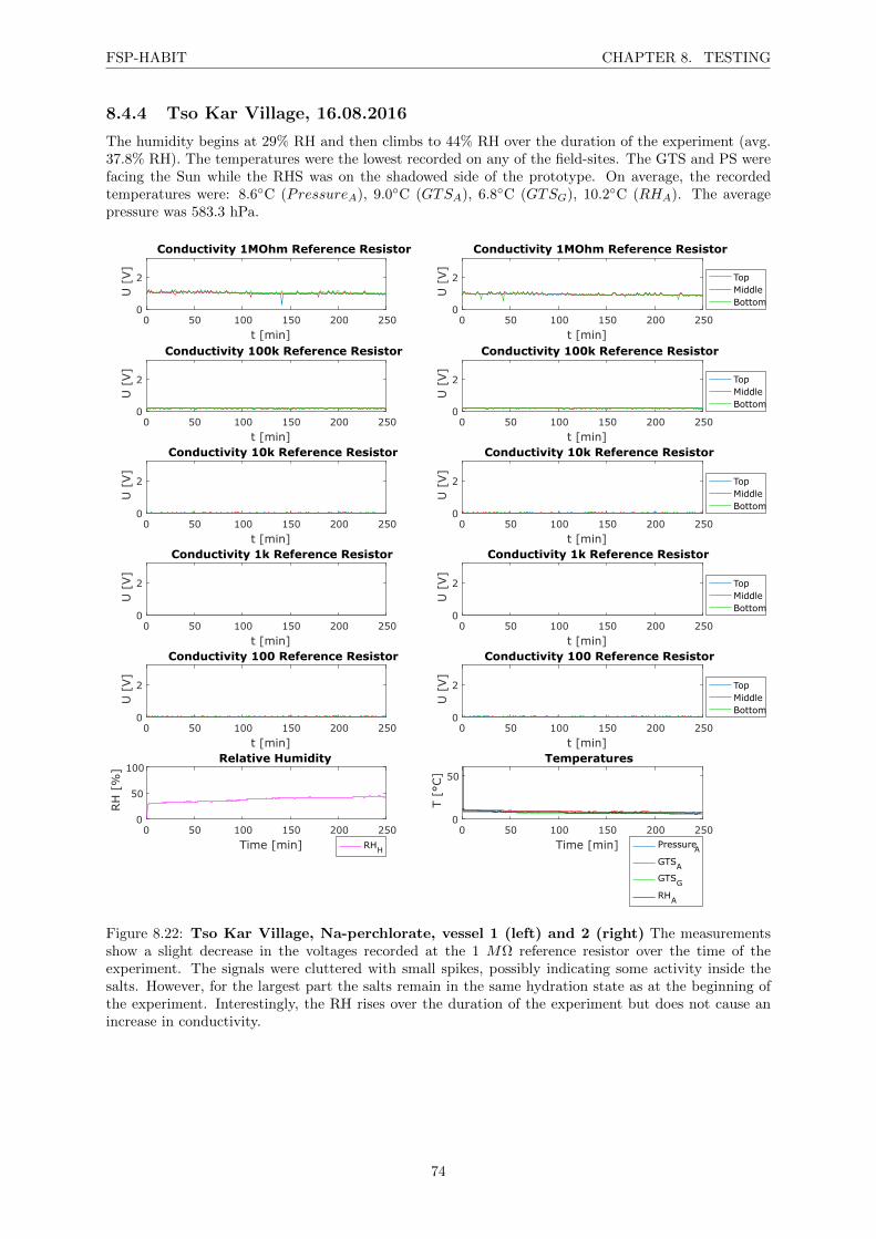
FSP-HABIT CHAPTER 8. TESTING
8.4.4 Tso Kar Village, 16.08.2016
The humidity begins at 29% RH and then climbs to 44% RH over the duration of the experiment (avg.37.8% RH). The temperatures were the lowest recorded on any of the field-sites. The GTS and PS werefacing the Sun while the RHS was on the shadowed side of the prototype. On average, the recordedtemperatures were: 8.6C (PressureA), 9.0C (GTSA), 6.8C (GTSG), 10.2C (RHA). The averagepressure was 583.3 hPa.
0 50 100 150 200 250
t [min]
0
2
U [
V]
Conductivity 1MOhm Reference Resistor
0 50 100 150 200 250
t [min]
0
2
U [
V]
Conductivity 100k Reference Resistor
0 50 100 150 200 250
t [min]
0
2
U [
V]
Conductivity 10k Reference Resistor
0 50 100 150 200 250
t [min]
0
2
U [
V]
Conductivity 1k Reference Resistor
0 50 100 150 200 250
t [min]
0
2
U [
V]
Conductivity 100 Reference Resistor
0 50 100 150 200 250
Time [min]
0
50
100
RH
[%
]
Relative Humidity
RHH
0 50 100 150 200 250
t [min]
0
2
U [
V]
Conductivity 1MOhm Reference Resistor
TopMiddleBottom
0 50 100 150 200 250
t [min]
0
2
U [
V]
Conductivity 100k Reference Resistor
TopMiddleBottom
0 50 100 150 200 250
t [min]
0
2
U [
V]
Conductivity 10k Reference Resistor
TopMiddleBottom
0 50 100 150 200 250
t [min]
0
2
U [
V]
Conductivity 1k Reference Resistor
TopMiddleBottom
0 50 100 150 200 250
t [min]
0
2
U [
V]
Conductivity 100 Reference Resistor
TopMiddleBottom
0 50 100 150 200 250
Time [min]
0
50
T [
°C]
Temperatures
PressureAGTSA
GTSG
RHA
Figure 8.22: Tso Kar Village, Na-perchlorate, vessel 1 (left) and 2 (right) The measurementsshow a slight decrease in the voltages recorded at the 1 MΩ reference resistor over the time of theexperiment. The signals were cluttered with small spikes, possibly indicating some activity inside thesalts. However, for the largest part the salts remain in the same hydration state as at the beginning ofthe experiment. Interestingly, the RH rises over the duration of the experiment but does not cause anincrease in conductivity.
74
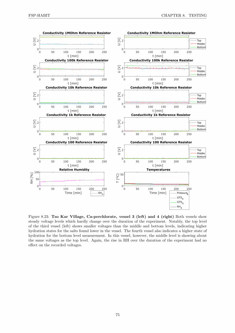
FSP-HABIT CHAPTER 8. TESTING
0 50 100 150 200 250
t [min]
0
2
U [
V]
Conductivity 1MOhm Reference Resistor
0 50 100 150 200 250
t [min]
0
2
U [
V]
Conductivity 100k Reference Resistor
0 50 100 150 200 250
t [min]
0
2
U [
V]
Conductivity 10k Reference Resistor
0 50 100 150 200 250
t [min]
0
2
U [
V]
Conductivity 1k Reference Resistor
0 50 100 150 200 250
t [min]
0
2
U [
V]
Conductivity 100 Reference Resistor
0 50 100 150 200 250
Time [min]
0
50
100
RH
[%
]
Relative Humidity
RHH
0 50 100 150 200 250
t [min]
0
2
U [
V]
Conductivity 1MOhm Reference Resistor
TopMiddleBottom
0 50 100 150 200 250
t [min]
0
2
U [
V]
Conductivity 100k Reference Resistor
TopMiddleBottom
0 50 100 150 200 250
t [min]
0
2
U [
V]
Conductivity 10k Reference Resistor
TopMiddleBottom
0 50 100 150 200 250
t [min]
0
2U
[V]
Conductivity 1k Reference Resistor
TopMiddleBottom
0 50 100 150 200 250
t [min]
0
2
U [
V]
Conductivity 100 Reference Resistor
TopMiddleBottom
0 50 100 150 200 250
Time [min]
0
50
T [
°C]
Temperatures
PressureAGTSA
GTSG
RHA
Figure 8.23: Tso Kar Village, Ca-perchlorate, vessel 3 (left) and 4 (right) Both vessels showsteady voltage levels which hardly change over the duration of the experiment. Notably, the top levelof the third vessel (left) shows smaller voltages than the middle and bottom levels, indicating higherhydration states for the salts found lower in the vessel. The fourth vessel also indicates a higher state ofhydration for the bottom level measurement. In this vessel, however, the middle level is showing aboutthe same voltages as the top level. Again, the rise in RH over the duration of the experiment had noeffect on the recorded voltages.
75
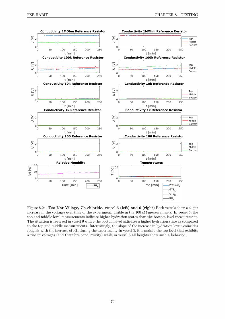
FSP-HABIT CHAPTER 8. TESTING
0 50 100 150 200 250
t [min]
0
2
U [
V]
Conductivity 1MOhm Reference Resistor
0 50 100 150 200 250
t [min]
0
2
U [
V]
Conductivity 100k Reference Resistor
0 50 100 150 200 250
t [min]
0
2
U [
V]
Conductivity 10k Reference Resistor
0 50 100 150 200 250
t [min]
0
2
U [
V]
Conductivity 1k Reference Resistor
0 50 100 150 200 250
t [min]
0
2
U [
V]
Conductivity 100 Reference Resistor
0 50 100 150 200 250
Time [min]
0
50
100
RH
[%
]
Relative Humidity
RHH
0 50 100 150 200 250
t [min]
0
2
U [
V]
Conductivity 1MOhm Reference Resistor
TopMiddleBottom
0 50 100 150 200 250
t [min]
0
2
U [
V]
Conductivity 100k Reference Resistor
TopMiddleBottom
0 50 100 150 200 250
t [min]
0
2
U [
V]
Conductivity 10k Reference Resistor
TopMiddleBottom
0 50 100 150 200 250
t [min]
0
2
U [
V]
Conductivity 1k Reference Resistor
TopMiddleBottom
0 50 100 150 200 250
t [min]
0
2
U [
V]
Conductivity 100 Reference Resistor
TopMiddleBottom
0 50 100 150 200 250
Time [min]
0
50
T [
°C]
Temperatures
PressureAGTSA
GTSG
RHA
Figure 8.24: Tso Kar Village, Ca-chloride, vessel 5 (left) and 6 (right) Both vessels show a slightincrease in the voltages over time of the experiment, visible in the 100 kΩ measurements. In vessel 5, thetop and middle level measurements indicate higher hydration states than the bottom level measurement.The situation is reversed in vessel 6 where the bottom level indicates a higher hydration state as comparedto the top and middle measurements. Interestingly, the slope of the increase in hydration levels coincidesroughly with the increase of RH during the experiment. In vessel 5, it is mainly the top level that exhibitsa rise in voltages (and therefore conductivity) while in vessel 6 all heights show such a behavior.
76
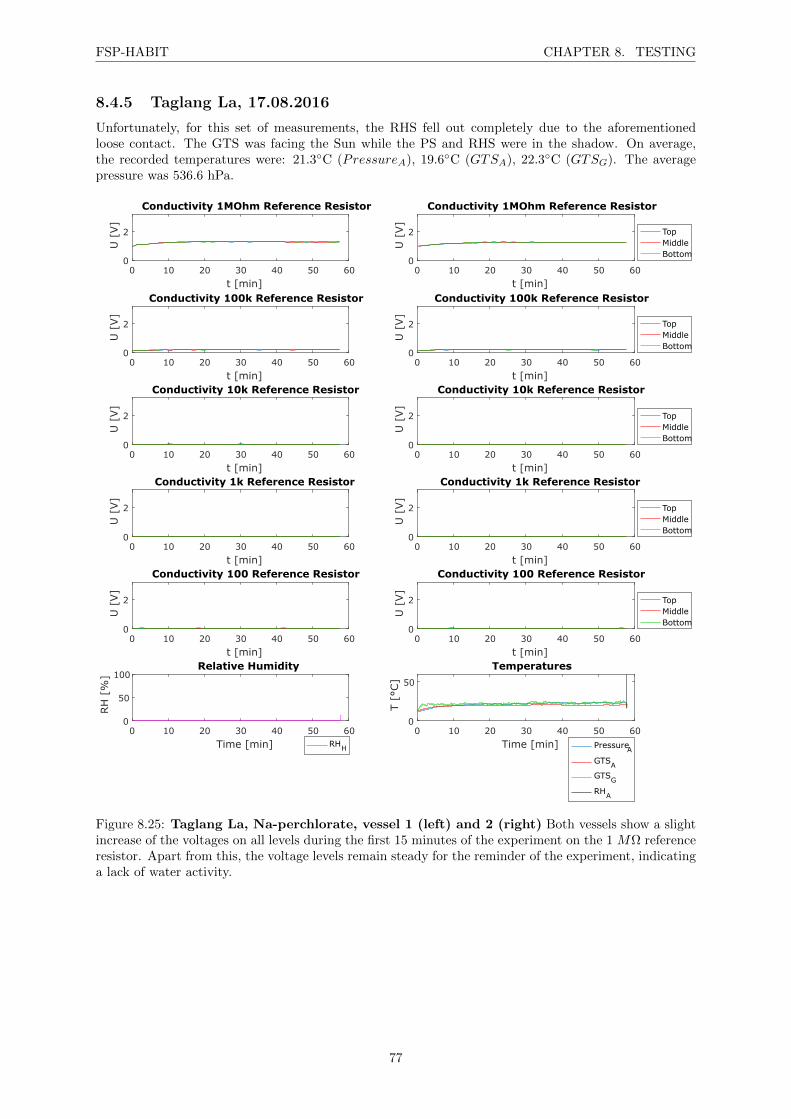
FSP-HABIT CHAPTER 8. TESTING
8.4.5 Taglang La, 17.08.2016
Unfortunately, for this set of measurements, the RHS fell out completely due to the aforementionedloose contact. The GTS was facing the Sun while the PS and RHS were in the shadow. On average,the recorded temperatures were: 21.3C (PressureA), 19.6C (GTSA), 22.3C (GTSG). The averagepressure was 536.6 hPa.
0 10 20 30 40 50 60
t [min]
0
2
U [
V]
Conductivity 1MOhm Reference Resistor
0 10 20 30 40 50 60
t [min]
0
2
U [
V]
Conductivity 100k Reference Resistor
0 10 20 30 40 50 60
t [min]
0
2
U [
V]
Conductivity 10k Reference Resistor
0 10 20 30 40 50 60
t [min]
0
2
U [
V]
Conductivity 1k Reference Resistor
0 10 20 30 40 50 60
t [min]
0
2
U [
V]
Conductivity 100 Reference Resistor
0 10 20 30 40 50 60
Time [min]
0
50
100
RH
[%
]
Relative Humidity
RHH
0 10 20 30 40 50 60
t [min]
0
2
U [
V]
Conductivity 1MOhm Reference Resistor
TopMiddleBottom
0 10 20 30 40 50 60
t [min]
0
2
U [
V]
Conductivity 100k Reference Resistor
TopMiddleBottom
0 10 20 30 40 50 60
t [min]
0
2
U [
V]
Conductivity 10k Reference Resistor
TopMiddleBottom
0 10 20 30 40 50 60
t [min]
0
2
U [
V]
Conductivity 1k Reference Resistor
TopMiddleBottom
0 10 20 30 40 50 60
t [min]
0
2
U [
V]
Conductivity 100 Reference Resistor
TopMiddleBottom
0 10 20 30 40 50 60
Time [min]
0
50
T [
°C]
Temperatures
PressureAGTSA
GTSG
RHA
Figure 8.25: Taglang La, Na-perchlorate, vessel 1 (left) and 2 (right) Both vessels show a slightincrease of the voltages on all levels during the first 15 minutes of the experiment on the 1 MΩ referenceresistor. Apart from this, the voltage levels remain steady for the reminder of the experiment, indicatinga lack of water activity.
77
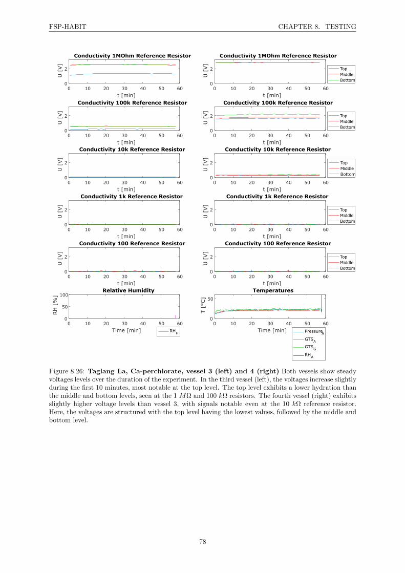
FSP-HABIT CHAPTER 8. TESTING
0 10 20 30 40 50 60
t [min]
0
2
U [
V]
Conductivity 1MOhm Reference Resistor
0 10 20 30 40 50 60
t [min]
0
2
U [
V]
Conductivity 100k Reference Resistor
0 10 20 30 40 50 60
t [min]
0
2
U [
V]
Conductivity 10k Reference Resistor
0 10 20 30 40 50 60
t [min]
0
2
U [
V]
Conductivity 1k Reference Resistor
0 10 20 30 40 50 60
t [min]
0
2
U [
V]
Conductivity 100 Reference Resistor
0 10 20 30 40 50 60
Time [min]
0
50
100
RH
[%
]
Relative Humidity
RHH
0 10 20 30 40 50 60
t [min]
0
2
U [
V]
Conductivity 1MOhm Reference Resistor
TopMiddleBottom
0 10 20 30 40 50 60
t [min]
0
2
U [
V]
Conductivity 100k Reference Resistor
TopMiddleBottom
0 10 20 30 40 50 60
t [min]
0
2
U [
V]
Conductivity 10k Reference Resistor
TopMiddleBottom
0 10 20 30 40 50 60
t [min]
0
2U
[V]
Conductivity 1k Reference Resistor
TopMiddleBottom
0 10 20 30 40 50 60
t [min]
0
2
U [
V]
Conductivity 100 Reference Resistor
TopMiddleBottom
0 10 20 30 40 50 60
Time [min]
0
50
T [
°C]
Temperatures
PressureAGTSA
GTSG
RHA
Figure 8.26: Taglang La, Ca-perchlorate, vessel 3 (left) and 4 (right) Both vessels show steadyvoltages levels over the duration of the experiment. In the third vessel (left), the voltages increase slightlyduring the first 10 minutes, most notable at the top level. The top level exhibits a lower hydration thanthe middle and bottom levels, seen at the 1 MΩ and 100 kΩ resistors. The fourth vessel (right) exhibitsslightly higher voltage levels than vessel 3, with signals notable even at the 10 kΩ reference resistor.Here, the voltages are structured with the top level having the lowest values, followed by the middle andbottom level.
78

FSP-HABIT CHAPTER 8. TESTING
0 10 20 30 40 50 60
t [min]
0
2
U [
V]
Conductivity 1MOhm Reference Resistor
0 10 20 30 40 50 60
t [min]
0
2
U [
V]
Conductivity 100k Reference Resistor
0 10 20 30 40 50 60
t [min]
0
2
U [
V]
Conductivity 10k Reference Resistor
0 10 20 30 40 50 60
t [min]
0
2
U [
V]
Conductivity 1k Reference Resistor
0 10 20 30 40 50 60
t [min]
0
2
U [
V]
Conductivity 100 Reference Resistor
0 10 20 30 40 50 60
Time [min]
0
50
100
RH
[%
]
Relative Humidity
RHH
0 10 20 30 40 50 60
t [min]
0
2
U [
V]
Conductivity 1MOhm Reference Resistor
TopMiddleBottom
0 10 20 30 40 50 60
t [min]
0
2
U [
V]
Conductivity 100k Reference Resistor
TopMiddleBottom
0 10 20 30 40 50 60
t [min]
0
2
U [
V]
Conductivity 10k Reference Resistor
TopMiddleBottom
0 10 20 30 40 50 60
t [min]
0
2U
[V]
Conductivity 1k Reference Resistor
TopMiddleBottom
0 10 20 30 40 50 60
t [min]
0
2
U [
V]
Conductivity 100 Reference Resistor
TopMiddleBottom
0 10 20 30 40 50 60
Time [min]
0
50
T [
°C]
Temperatures
PressureAGTSA
GTSG
RHA
Figure 8.27: Taglang La, Ca-chloride, vessel 5 (left) and 6 (right) Both vessels show relativelystable voltages at all levels. However, vessel 5 (left) shows decreasing voltages on the top and middlelevels for the 1 MΩ resistor over the duration of the experiment. At vessel 6 (right), on the other hand,only the top level measurement decreases over the time of the experiment, visible at the 1 MΩ and atthe 100 kΩ reference resistors. This could indicate a mild drying process at the top levels of the salts.
79
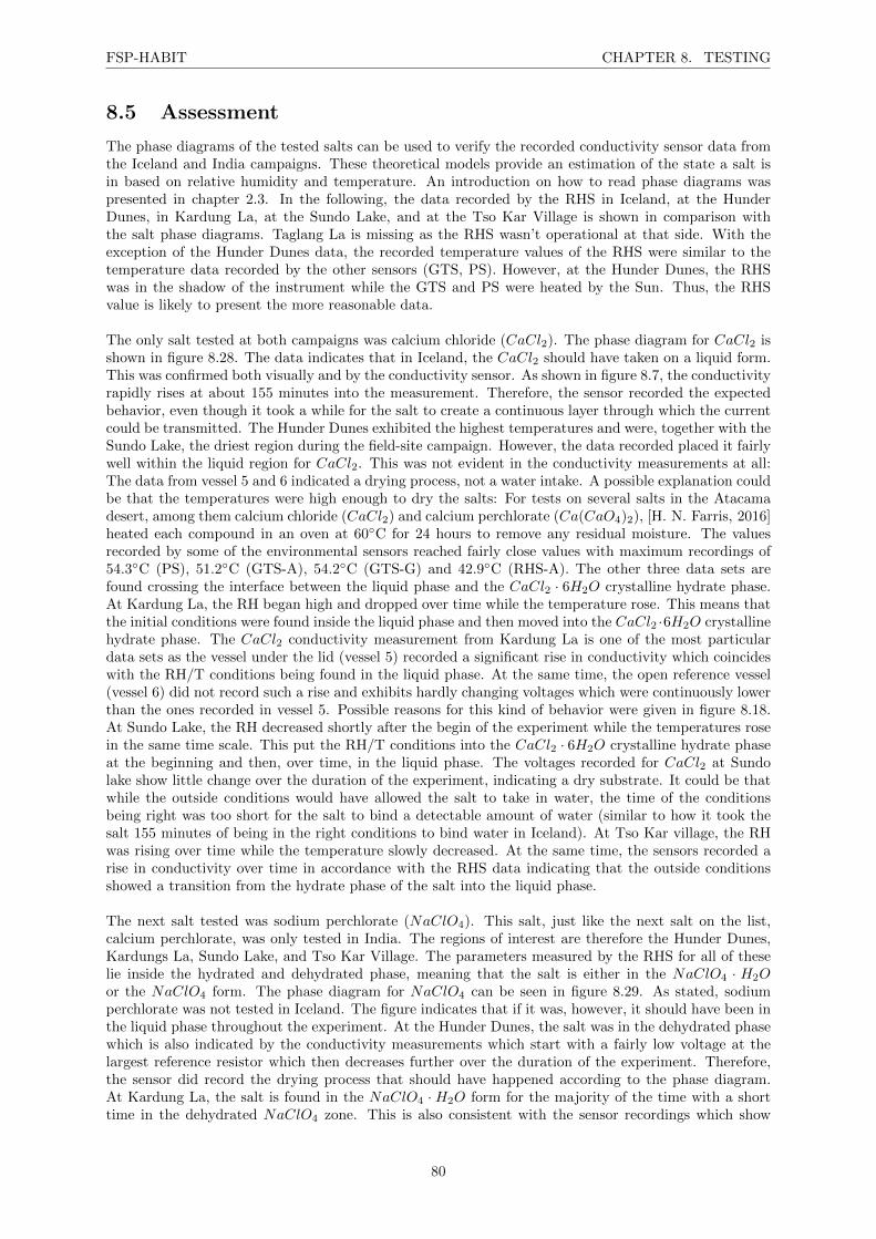
FSP-HABIT CHAPTER 8. TESTING
8.5 Assessment
The phase diagrams of the tested salts can be used to verify the recorded conductivity sensor data fromthe Iceland and India campaigns. These theoretical models provide an estimation of the state a salt isin based on relative humidity and temperature. An introduction on how to read phase diagrams waspresented in chapter 2.3. In the following, the data recorded by the RHS in Iceland, at the HunderDunes, in Kardung La, at the Sundo Lake, and at the Tso Kar Village is shown in comparison withthe salt phase diagrams. Taglang La is missing as the RHS wasn’t operational at that side. With theexception of the Hunder Dunes data, the recorded temperature values of the RHS were similar to thetemperature data recorded by the other sensors (GTS, PS). However, at the Hunder Dunes, the RHSwas in the shadow of the instrument while the GTS and PS were heated by the Sun. Thus, the RHSvalue is likely to present the more reasonable data.
The only salt tested at both campaigns was calcium chloride (CaCl2). The phase diagram for CaCl2 isshown in figure 8.28. The data indicates that in Iceland, the CaCl2 should have taken on a liquid form.This was confirmed both visually and by the conductivity sensor. As shown in figure 8.7, the conductivityrapidly rises at about 155 minutes into the measurement. Therefore, the sensor recorded the expectedbehavior, even though it took a while for the salt to create a continuous layer through which the currentcould be transmitted. The Hunder Dunes exhibited the highest temperatures and were, together with theSundo Lake, the driest region during the field-site campaign. However, the data recorded placed it fairlywell within the liquid region for CaCl2. This was not evident in the conductivity measurements at all:The data from vessel 5 and 6 indicated a drying process, not a water intake. A possible explanation couldbe that the temperatures were high enough to dry the salts: For tests on several salts in the Atacamadesert, among them calcium chloride (CaCl2) and calcium perchlorate (Ca(CaO4)2), [H. N. Farris, 2016]heated each compound in an oven at 60C for 24 hours to remove any residual moisture. The valuesrecorded by some of the environmental sensors reached fairly close values with maximum recordings of54.3C (PS), 51.2C (GTS-A), 54.2C (GTS-G) and 42.9C (RHS-A). The other three data sets arefound crossing the interface between the liquid phase and the CaCl2 · 6H2O crystalline hydrate phase.At Kardung La, the RH began high and dropped over time while the temperature rose. This means thatthe initial conditions were found inside the liquid phase and then moved into the CaCl2 ·6H2O crystallinehydrate phase. The CaCl2 conductivity measurement from Kardung La is one of the most particulardata sets as the vessel under the lid (vessel 5) recorded a significant rise in conductivity which coincideswith the RH/T conditions being found in the liquid phase. At the same time, the open reference vessel(vessel 6) did not record such a rise and exhibits hardly changing voltages which were continuously lowerthan the ones recorded in vessel 5. Possible reasons for this kind of behavior were given in figure 8.18.At Sundo Lake, the RH decreased shortly after the begin of the experiment while the temperatures rosein the same time scale. This put the RH/T conditions into the CaCl2 · 6H2O crystalline hydrate phaseat the beginning and then, over time, in the liquid phase. The voltages recorded for CaCl2 at Sundolake show little change over the duration of the experiment, indicating a dry substrate. It could be thatwhile the outside conditions would have allowed the salt to take in water, the time of the conditionsbeing right was too short for the salt to bind a detectable amount of water (similar to how it took thesalt 155 minutes of being in the right conditions to bind water in Iceland). At Tso Kar village, the RHwas rising over time while the temperature slowly decreased. At the same time, the sensors recorded arise in conductivity over time in accordance with the RHS data indicating that the outside conditionsshowed a transition from the hydrate phase of the salt into the liquid phase.
The next salt tested was sodium perchlorate (NaClO4). This salt, just like the next salt on the list,calcium perchlorate, was only tested in India. The regions of interest are therefore the Hunder Dunes,Kardungs La, Sundo Lake, and Tso Kar Village. The parameters measured by the RHS for all of theselie inside the hydrated and dehydrated phase, meaning that the salt is either in the NaClO4 · H2Oor the NaClO4 form. The phase diagram for NaClO4 can be seen in figure 8.29. As stated, sodiumperchlorate was not tested in Iceland. The figure indicates that if it was, however, it should have been inthe liquid phase throughout the experiment. At the Hunder Dunes, the salt was in the dehydrated phasewhich is also indicated by the conductivity measurements which start with a fairly low voltage at thelargest reference resistor which then decreases further over the duration of the experiment. Therefore,the sensor did record the drying process that should have happened according to the phase diagram.At Kardung La, the salt is found in the NaClO4 ·H2O form for the majority of the time with a shorttime in the dehydrated NaClO4 zone. This is also consistent with the sensor recordings which show
80
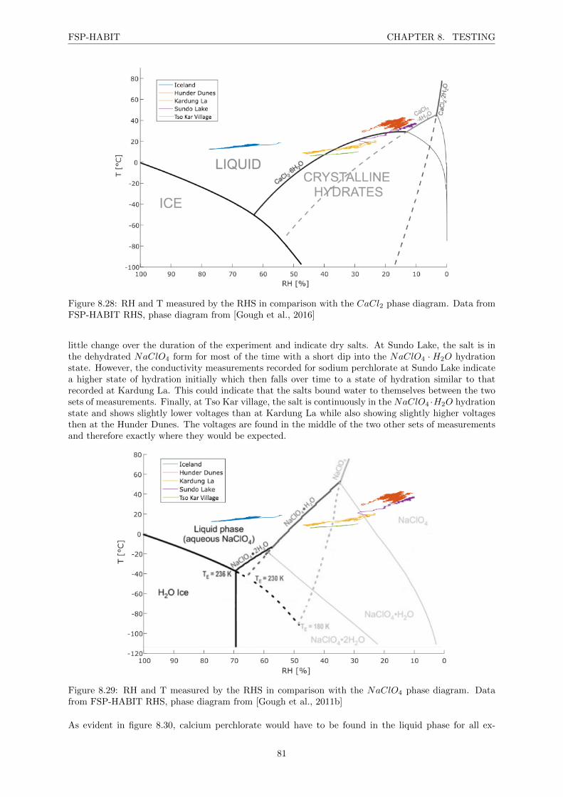
FSP-HABIT CHAPTER 8. TESTING
Figure 8.28: RH and T measured by the RHS in comparison with the CaCl2 phase diagram. Data fromFSP-HABIT RHS, phase diagram from [Gough et al., 2016]
little change over the duration of the experiment and indicate dry salts. At Sundo Lake, the salt is inthe dehydrated NaClO4 form for most of the time with a short dip into the NaClO4 ·H2O hydrationstate. However, the conductivity measurements recorded for sodium perchlorate at Sundo Lake indicatea higher state of hydration initially which then falls over time to a state of hydration similar to thatrecorded at Kardung La. This could indicate that the salts bound water to themselves between the twosets of measurements. Finally, at Tso Kar village, the salt is continuously in the NaClO4 ·H2O hydrationstate and shows slightly lower voltages than at Kardung La while also showing slightly higher voltagesthen at the Hunder Dunes. The voltages are found in the middle of the two other sets of measurementsand therefore exactly where they would be expected.
Figure 8.29: RH and T measured by the RHS in comparison with the NaClO4 phase diagram. Datafrom FSP-HABIT RHS, phase diagram from [Gough et al., 2011b]
As evident in figure 8.30, calcium perchlorate would have to be found in the liquid phase for all ex-
81
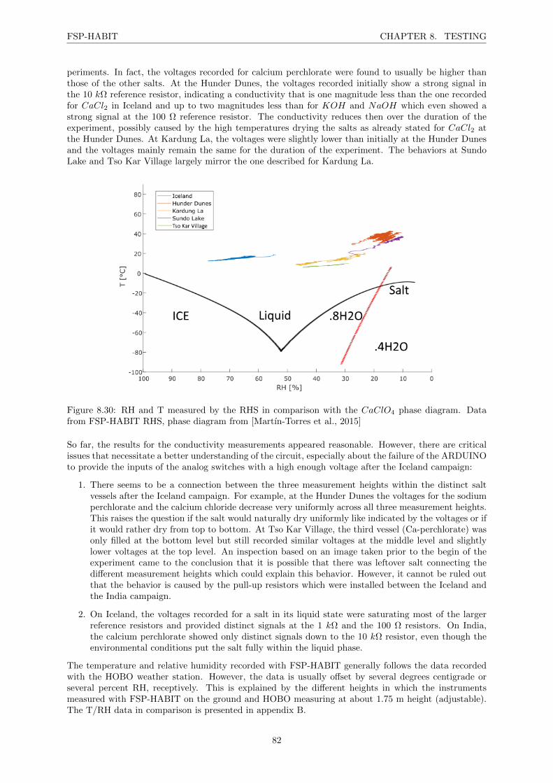
FSP-HABIT CHAPTER 8. TESTING
periments. In fact, the voltages recorded for calcium perchlorate were found to usually be higher thanthose of the other salts. At the Hunder Dunes, the voltages recorded initially show a strong signal inthe 10 kΩ reference resistor, indicating a conductivity that is one magnitude less than the one recordedfor CaCl2 in Iceland and up to two magnitudes less than for KOH and NaOH which even showed astrong signal at the 100 Ω reference resistor. The conductivity reduces then over the duration of theexperiment, possibly caused by the high temperatures drying the salts as already stated for CaCl2 atthe Hunder Dunes. At Kardung La, the voltages were slightly lower than initially at the Hunder Dunesand the voltages mainly remain the same for the duration of the experiment. The behaviors at SundoLake and Tso Kar Village largely mirror the one described for Kardung La.
Figure 8.30: RH and T measured by the RHS in comparison with the CaClO4 phase diagram. Datafrom FSP-HABIT RHS, phase diagram from [Martın-Torres et al., 2015]
So far, the results for the conductivity measurements appeared reasonable. However, there are criticalissues that necessitate a better understanding of the circuit, especially about the failure of the ARDUINOto provide the inputs of the analog switches with a high enough voltage after the Iceland campaign:
1. There seems to be a connection between the three measurement heights within the distinct saltvessels after the Iceland campaign. For example, at the Hunder Dunes the voltages for the sodiumperchlorate and the calcium chloride decrease very uniformly across all three measurement heights.This raises the question if the salt would naturally dry uniformly like indicated by the voltages or ifit would rather dry from top to bottom. At Tso Kar Village, the third vessel (Ca-perchlorate) wasonly filled at the bottom level but still recorded similar voltages at the middle level and slightlylower voltages at the top level. An inspection based on an image taken prior to the begin of theexperiment came to the conclusion that it is possible that there was leftover salt connecting thedifferent measurement heights which could explain this behavior. However, it cannot be ruled outthat the behavior is caused by the pull-up resistors which were installed between the Iceland andthe India campaign.
2. On Iceland, the voltages recorded for a salt in its liquid state were saturating most of the largerreference resistors and provided distinct signals at the 1 kΩ and the 100 Ω resistors. On India,the calcium perchlorate showed only distinct signals down to the 10 kΩ resistor, even though theenvironmental conditions put the salt fully within the liquid phase.
The temperature and relative humidity recorded with FSP-HABIT generally follows the data recordedwith the HOBO weather station. However, the data is usually offset by several degrees centigrade orseveral percent RH, receptively. This is explained by the different heights in which the instrumentsmeasured with FSP-HABIT on the ground and HOBO measuring at about 1.75 m height (adjustable).The T/RH data in comparison is presented in appendix B.
82
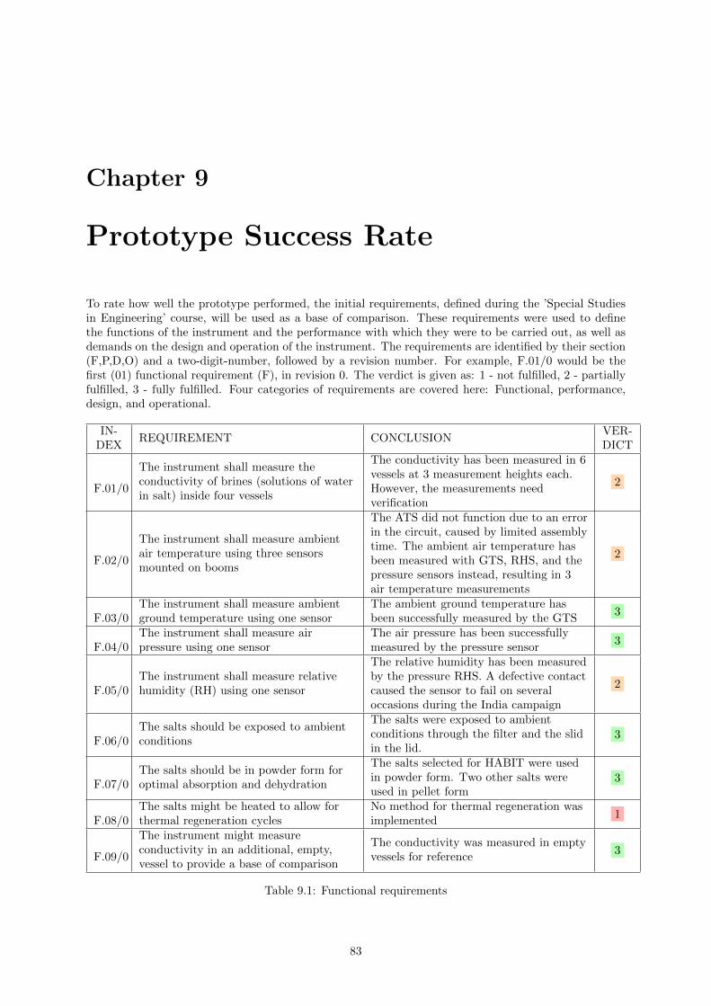
Chapter 9
Prototype Success Rate
To rate how well the prototype performed, the initial requirements, defined during the ’Special Studiesin Engineering’ course, will be used as a base of comparison. These requirements were used to definethe functions of the instrument and the performance with which they were to be carried out, as well asdemands on the design and operation of the instrument. The requirements are identified by their section(F,P,D,O) and a two-digit-number, followed by a revision number. For example, F.01/0 would be thefirst (01) functional requirement (F), in revision 0. The verdict is given as: 1 - not fulfilled, 2 - partiallyfulfilled, 3 - fully fulfilled. Four categories of requirements are covered here: Functional, performance,design, and operational.
IN-DEX
REQUIREMENT CONCLUSIONVER-DICT
F.01/0
The instrument shall measure theconductivity of brines (solutions of waterin salt) inside four vessels
The conductivity has been measured in 6vessels at 3 measurement heights each.However, the measurements needverification
2
F.02/0
The instrument shall measure ambientair temperature using three sensorsmounted on booms
The ATS did not function due to an errorin the circuit, caused by limited assemblytime. The ambient air temperature hasbeen measured with GTS, RHS, and thepressure sensors instead, resulting in 3air temperature measurements
2
F.03/0The instrument shall measure ambientground temperature using one sensor
The ambient ground temperature hasbeen successfully measured by the GTS
3
F.04/0The instrument shall measure airpressure using one sensor
The air pressure has been successfullymeasured by the pressure sensor
3
F.05/0The instrument shall measure relativehumidity (RH) using one sensor
The relative humidity has been measuredby the pressure RHS. A defective contactcaused the sensor to fail on severaloccasions during the India campaign
2
F.06/0The salts should be exposed to ambientconditions
The salts were exposed to ambientconditions through the filter and the slidin the lid.
3
F.07/0The salts should be in powder form foroptimal absorption and dehydration
The salts selected for HABIT were usedin powder form. Two other salts wereused in pellet form
3
F.08/0The salts might be heated to allow forthermal regeneration cycles
No method for thermal regeneration wasimplemented
1
F.09/0
The instrument might measureconductivity in an additional, empty,vessel to provide a base of comparison
The conductivity was measured in emptyvessels for reference
3
Table 9.1: Functional requirements
83
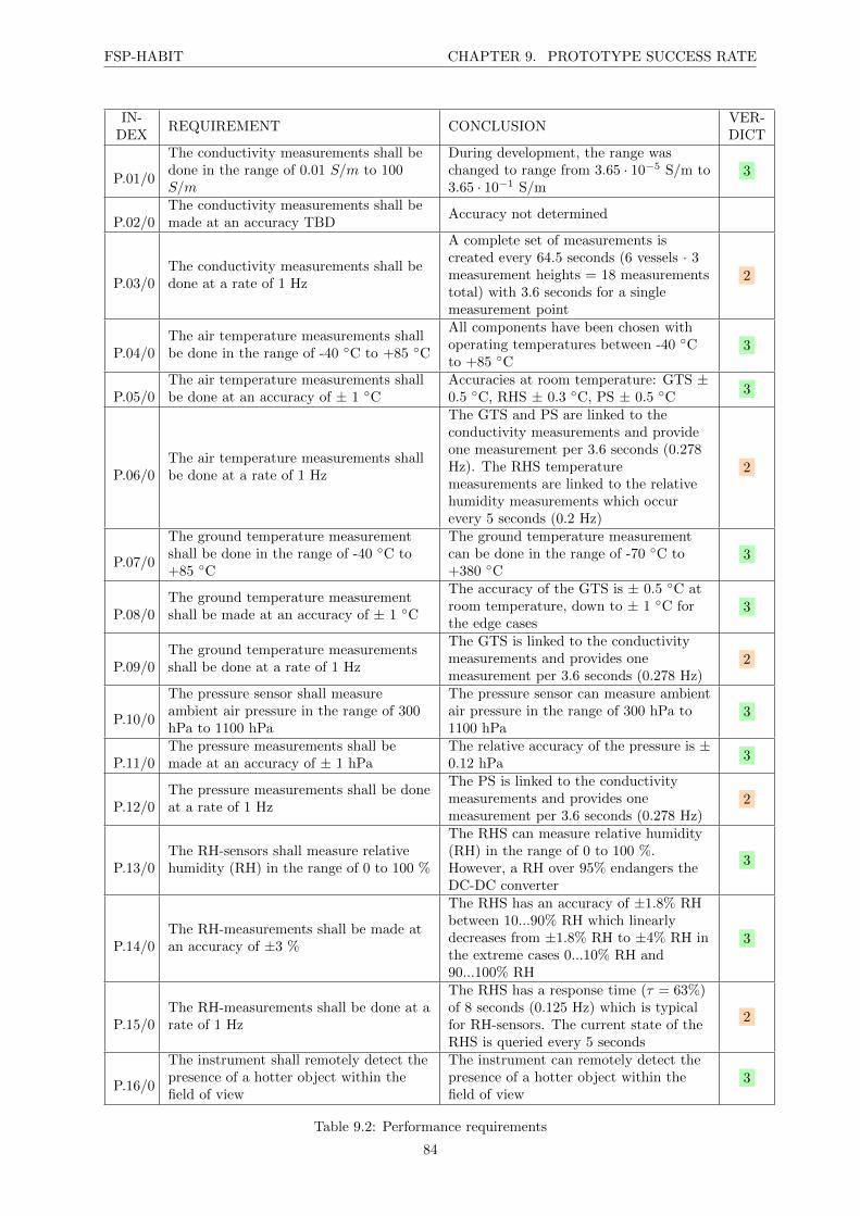
FSP-HABIT CHAPTER 9. PROTOTYPE SUCCESS RATE
IN-DEX
REQUIREMENT CONCLUSIONVER-DICT
P.01/0
The conductivity measurements shall bedone in the range of 0.01 S/m to 100S/m
During development, the range waschanged to range from 3.65 · 10−5 S/m to3.65 · 10−1 S/m
3
P.02/0The conductivity measurements shall bemade at an accuracy TBD
Accuracy not determined
P.03/0The conductivity measurements shall bedone at a rate of 1 Hz
A complete set of measurements iscreated every 64.5 seconds (6 vessels · 3measurement heights = 18 measurementstotal) with 3.6 seconds for a singlemeasurement point
2
P.04/0The air temperature measurements shallbe done in the range of -40 C to +85 C
All components have been chosen withoperating temperatures between -40 Cto +85 C
3
P.05/0The air temperature measurements shallbe done at an accuracy of ± 1 C
Accuracies at room temperature: GTS ±0.5 C, RHS ± 0.3 C, PS ± 0.5 C
3
P.06/0The air temperature measurements shallbe done at a rate of 1 Hz
The GTS and PS are linked to theconductivity measurements and provideone measurement per 3.6 seconds (0.278Hz). The RHS temperaturemeasurements are linked to the relativehumidity measurements which occurevery 5 seconds (0.2 Hz)
2
P.07/0
The ground temperature measurementshall be done in the range of -40 C to+85 C
The ground temperature measurementcan be done in the range of -70 C to+380 C
3
P.08/0The ground temperature measurementshall be made at an accuracy of ± 1 C
The accuracy of the GTS is ± 0.5 C atroom temperature, down to ± 1 C forthe edge cases
3
P.09/0The ground temperature measurementsshall be done at a rate of 1 Hz
The GTS is linked to the conductivitymeasurements and provides onemeasurement per 3.6 seconds (0.278 Hz)
2
P.10/0
The pressure sensor shall measureambient air pressure in the range of 300hPa to 1100 hPa
The pressure sensor can measure ambientair pressure in the range of 300 hPa to1100 hPa
3
P.11/0The pressure measurements shall bemade at an accuracy of ± 1 hPa
The relative accuracy of the pressure is ±0.12 hPa
3
P.12/0The pressure measurements shall be doneat a rate of 1 Hz
The PS is linked to the conductivitymeasurements and provides onemeasurement per 3.6 seconds (0.278 Hz)
2
P.13/0The RH-sensors shall measure relativehumidity (RH) in the range of 0 to 100 %
The RHS can measure relative humidity(RH) in the range of 0 to 100 %.However, a RH over 95% endangers theDC-DC converter
3
P.14/0The RH-measurements shall be made atan accuracy of ±3 %
The RHS has an accuracy of ±1.8% RHbetween 10...90% RH which linearlydecreases from ±1.8% RH to ±4% RH inthe extreme cases 0...10% RH and90...100% RH
3
P.15/0The RH-measurements shall be done at arate of 1 Hz
The RHS has a response time (τ = 63%)of 8 seconds (0.125 Hz) which is typicalfor RH-sensors. The current state of theRHS is queried every 5 seconds
2
P.16/0
The instrument shall remotely detect thepresence of a hotter object within thefield of view
The instrument can remotely detect thepresence of a hotter object within thefield of view
3
Table 9.2: Performance requirements
84

FSP-HABIT CHAPTER 9. PROTOTYPE SUCCESS RATE
IN-DEX
REQUIREMENT CONCLUSIONVER-DICT
D.01/0
The instrument shall operate intemperatures found under laboratoryconditions
The instrument can operate intemperatures found under laboratoryconditions
3
D.02/0
The instrument shall operate intemperatures found during winter inNorrbotten county, northern Sweden
The instrument was not tested undersuch conditions. However, componentshave been selected to allow for coldtemperatures
3
D.03/0
The instrument shall operate intemperatures found during summer inthe Himalaya, India, at high altitudes
The instrumented operated under thestated conditions. The prolongedexposure to high temperatures deformedthe PLA of the EBox Assembly
2
D.04/0
The instrument shall operate intemperatures found during summer inIceland, close to volcanic areas
The instrument operated under thestated conditions
3
D.05/0The instrument batteries shall berechargeable
The batteries can be exchanged with theoption to use rechargeable batteries
3
D.06/0
The instrument batteries shall providepower for at least 24 hours of continuousmeasurements
The instrument was run at longest for 4h 10 min during the India campaign. Thebatteries are estimated to last at least 10hours for NiMh batteries above 0C
2
D.07/0The salt vessels shall contain the salts The salt vessels can contain the salts 3
D.08/0The salt vessels shall not leak water The salt vessels do not leak water 3
D.09/0The salt vessel filters shall only letthrough air
The salt vessel filters prevent particlesbigger 0.2 µm from entering the brinevessels (= salt vessels)
3
D.10/0The salt vessel filters shall enduretransportation
The salt vessel filters can enduretransportation
3
D.11/0The salt vessel filters shall not react withthe salts
The salt vessel filters did not react withthe salts
3
D.12/0The conductivity sensor material shallnot react with the salts
The electrodes suffered minimal corrosion 3
D.13/0The salt vessel material shall not reactwith the salts
The brine vessel walls did not reactvisibly with salts
3
D.14/0The measured data shall be saved to astorage device with a frequency TBD
The measured data has been saved to aSD card every 3.6 seconds
3
D.14/0
The instrument should beassembled/disassembled to anoperational/transportable state within 10minutes
The instrument can beassembled/disassembled to anoperational/transportable state within 10minutes
3
Table 9.3: Design requirements
85
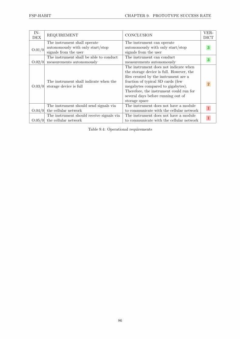
FSP-HABIT CHAPTER 9. PROTOTYPE SUCCESS RATE
IN-DEX
REQUIREMENT CONCLUSIONVER-DICT
O.01/0
The instrument shall operateautonomously with only start/stopsignals from the user
The instrument can operateautonomously with only start/stopsignals from the user
3
O.02/0The instrument shall be able to conductmeasurements autonomously
The instrument can conductmeasurements autonomously
3
O.03/0The instrument shall indicate when thestorage device is full
The instrument does not indicate whenthe storage device is full. However, thefiles created by the instrument are afraction of typical SD cards (fewmegabytes compared to gigabytes).Therefore, the instrument could run forseveral days before running out ofstorage space
2
O.04/0The instrument should send signals viathe cellular network
The instrument does not have a moduleto communicate with the cellular network
1
O.05/0The instrument should receive signals viathe cellular network
The instrument does not have a moduleto communicate with the cellular network
1
Table 9.4: Operational requirements
86

Chapter 10
Conclusions And Outlook
During the development of FSP-HABIT, several key steps have been performed. The mechanical designof the brines container assembly (BCA) went through several iterations and now consists of six individ-ual parts. Special effort was put into creating fully functional salt vessels with easily interchangeableelectrodes in order to battle corrosion affecting the measurements. The electrodes offer three distinctmeasurement heights to better analyze the salt behavior and were chosen with two different surfacefinishes: ENIG and ENEPIG. The BCA features cable management in the form of the Cable Canal andATS Mount (CCAM) which leads the cables from the Brines Container towards the EBox while offeringsome protection from the environment. The CCAM also comes with three 40.0 mm protrusions withinwhich the Pt1000 air temperature sensors (ATS) are found. Membrane filters, placed above the saltswith a fixture, protect the salts from particles during the operation while still allowing water to passthrough. Finally, a lid allows for air to slowly flow over the salts while preventing direct Sun light tointeract with the salts and offers additional protection from particles. The Electronics Box Assembly(EBox) is merged with the BCA by two screws, elevating the BCA 20.0 mm above the ground to reducethermal interaction between the BCA and the ground affecting the salts’ behavior. The EBox itself ismade from two parts, the EBox Main and the EBox Lid. The Main holds the majority of the electronicsin the form of the circuit board. It also provides individually designed mounts for the GTS and the RHS,mounting spots for the circuit board and for the legs, and some structures for cable management. TheLid holds the ARDUINO, the batteries, a small circuit board for the SD-Card reader and the DC-DCconverter, and a mount for the PS.
For the electrical design several commercial sensors were implemented, namely an infra red Ground Tem-perature Sensor (GTS), a Relative Humidity Sensor (RHS), and a Pressure Sensor (PS), all includingtheir respective circuitry. For the three Pt1000 sensors making up the Air Temperature Sensor (ATS), acircuit created by P. Wittmann as part of his Masters thesis was placed onto the circuit board. Unfor-tunately, a lack of time during the assembly prevented a successful implementation of the circuit. TheElectric Conductivity Sensor was developed from scratch and consists of several components: The ACsignal generator creates a 1 kHz ±5 V signal which is then led to the 18 electrode measurement pointsby use of several analog switches. Between the salts and six (separately selectable) reference resistors avoltage division takes place. The result of this division is run through a precision full-wave rectifier sothat it can be safely read out by the ARDUINO. Voltage followers provide high input impedances andlow output impedances during the process.
On the software side, a program to run all sensors and store their data has been written and saved ontothe ARDUINO. The program was comprised of software libraries for the commercial components withcorresponding call functions. The data storing format was created specifically for FSP-HABIT as wasthe software for the electric conductivity sensor.The prototype performed well in several categories (GTS, PS, BCA, electrodes, batteries, SD storage)while showing issues in others (conductivity measurements for 18 points, EBox assembly, loose contactat RHS). For future iterations the following steps could be taken (in no particular order):
More laboratory tests and system level tests: While the prototype reached a level whichresembled a functioning system within three months, more time should be allocated for the assemblyof the prototype and subsequent system level testing. The prototype was completely assembledwithin the last two weeks prior to the Iceland campaign. This included the 3D-printing of the
87
FSP-HABIT CHAPTER 10. CONCLUSIONS AND OUTLOOK
EBox assembly and parts of the BCA, the soldering of the electronic components onto the circuitboard, including the circuit for the ATS (which was developed by P. Wittmann separately), allof the necessary wiring, the preparation of the electrodes (involving filing and soldering), andthe combination of all parts to form a complete instrument. Especially the 3D-printing and thesoldering took more time then anticipated: The 3D-printing process had to be restarted severaltimes for almost every part that was printed due to issues with the printer. Parts that wouldtake up to more than 24 hours to print would be irreversibly destroyed due to either issues withthe material feeder or the material heating nozzle. The soldering will be covered under ’PCB’.Doubling the time for assembly to 4 weeks would probably have been sufficient. The assembly forthe Iceland campaign was stopped in the last possible moment before packing the prototype forshipping. Sadly, this meant that there was no time left for system level tests of any sort. Thesetests could have showed issues with the prototype prior to the campaigns and would have allowedtime to characterize the behavior of the instrument under laboratory conditions. At the same time,scheduling some additional time for adjustments and/or fixes would have ensured a more reliableinstrument. Another month of tests might have done the trick. In the end, another 1.5 months fortesting would have benefited the prototype in preparing it for deployment on field-site campaigns.
PCB: The electronics of FSP-HABIT were soldered on a three-hole experiment circuit boardwhich necessitated hand-soldering a multitude of connections. The large amount of connectionsand having several different circuits including 3.3 V (ENVPACK) and 5 V (BOTTLE) supplies,combined with the aforementioned lack of time during assembly created a source of errors whichultimately led to the ATS circuit being nonoperational and the conductivity/BOTTLE circuit beingless reliable. At the time, it was decided to use the circuit board as it was thought that it wouldallow greater flexibility for changes should they become necessary and due to time constraints. Aprinted circuit board (PCB) would have taken extra time to be developed in programs like EAGLEand would then have to be manufactured by an external supplier and shipped to the campus. Analternative would have been to use copper plates and etch the circuit into it. However, this hasnot been done before by the author and held the risk for further delays which were unacceptableas there was little time for trying out the method. Nonetheless, a PCB could greatly decrease thesources for errors during the soldering process by reducing the number of soldering points. It wouldalso ensure a more homogeneous distribution of solder since the need for bridging solder points forsome connections would be removed. Finally, it could, potentially, reduce the form factor of thecircuit board and, thus, reduce the size of the EBox assembly.
Housing: During assembly it became evident that the amount of space allocated for cable man-agement was the minimum amount needed to squeeze the cables into the different housings (BCAand EBox). This was partly due to using single core wires which are fairly stiff but easy to solder.The space allocated for cables should therefore be increased by 20-40%. Another improvement,especially when considering potential runs in very cold environments, would be to install a layerof insulation, for example out of polystyrene, to the prototype. An issue that should definitelybe looked at is the mount for the RHS. The current implementation should be enhanced with astructure that holds the connection between the RHS and the cables leading away from it to thecircuit board in place. A lack of such a structure caused the RHS to fail on several occasions andthus should be fixed.
Circuit Improvements: The circuit’s accuracy could be improved by adding a system for syn-chronous demodulation (SD) to it. SD is typically used to extract weak signals against strong noisebackgrounds and filters the measured signal by using a reference signal. The part of the measuredsignal that has the same frequency and phase as the reference signal will be amplified. This wouldbe a viable technique for FSP-HABIT since the reference signal would be the signal generated bythe signal generator and, thus, has to be created anyway. SD has been used for the Phoenix TECP[Zent et al., 2009] and proofed to be a good way to increase the Signal-to-Noise ratio.
Clock: Currently, the prototype requires the operator to mark down the time of the begin of theexperiments manually. This means that the data recorded has to be seen in combination withother documentation to make the most use of the data. A solution could be a clock, powered byan independent battery, which would then provide time stamps for the data. An example for asimple implementation would be the Adafruit DS1307 real time clock breakout board kit. The kitis similarly easy to install as other breakout boards from Adafruit and is powered by a CR1220coin cell battery. According to the supplier, it will keep time for five years or more.
88

FSP-HABIT CHAPTER 10. CONCLUSIONS AND OUTLOOK
Easier access to the salts: As explained in the mechanical design sections, the BCA is heldtogether by six screws. While proofing to be functional during the campaigns, it also means thatthe brines container is disconnected from the CCAM every time the salts are exchanged (once perday during the campaigns). The BCA could be redesigned so that the filter fixation, filter mount,and lid can be removed from the BCA independently to allow access to the brine containers withoutthe need to disconnect the brines container from the CCAM.
Two RHS: RH measurements, in conjunction with temperature measurements, are a critical toolto evaluate the changes in conductivity in the brine containers. During the India campaign, theRHS failed on several occasions due to a loose contact. Also, both during the India and the Icelandcampaign, it could be seen that the measurements are sensitive to the influence of sunlight. Usingtwo RHS on opposite sides of the prototype would not only counter the effects of sunlight butwould also provide a backup for measuring this important parameter.
Long-term salt tests: The salts were always inserted into the vessels prior to the measurements,both during the campaigns and during laboratory tests. However, it would also be interesting to seeexactly which form the salts will take once they went through a full hydration/dehydration cycle.In their initial form when bought, the salts are typically a more or less coarse powder, dependingon the salt. After the laboratory tests, however, sometimes the salts would stick on the walls ofthe used beakers, proofing to be hard to remove. It should therefore be studied whether the saltsreturn to a powdery form after a cycle or if they take other forms, for example appear more like asolid crystal (which would limit the area of interaction with the atmosphere).
Material: While the PLA did its job in holding together the prototype, the EBox assemblyshowed some deformations after the India campaign. These were possibly caused by a combinationof direct heating through the sunlight and some design flaws such as the very limited space insidethe prototype, squeezing some of the cables which then in turn pressed against the housing. At thesame time, the wide spacing between the legs for the thermal decoupling caused a sinking of themiddle part of the EBox. This showed that the material is not stable enough to work well with thecurrent design in hot temperatures. Steps against this would be a material change or an update ofthe mechanical design.
Flat filter fixation: In its current implementation the filter fixation is basically a coarse grid.This leads to the issue that dust can accumulate on top of the filters and, due to the structure ofthe fixation, cannot be easily carried away by wind flow. By removing parts of the grid, this effectcould be made less severe. However, this would probably come at the cost of mechanical stability.
In conclusion, the prototype was brought to a good level considering the amount of sensors included,the development of the electrical/mechanical/software design from scratch, and the given time-frame. Itmarks an important first step in the development of further field-site prototypes. These further prototypescould aim to improve the conductivity measurements at 18 points and implement the improvements statedabove. The author wishes the LTU Atmospheric Science Group the best of luck in creating amazingscientific instruments surrounding the HABIT project.
89
Bibliography
[Analytical, 2004] Analytical, R. (2004). Conductivity - Theory and Practice [Application data sheet].Radiometer Analytical SAS [company].
[Andrews, 2010] Andrews, D. G. (2010). An Introduction to Atmospheric Physics. Second Edition. Cam-bridge University Press, Cambridge, UK.
[Bard and Faulkner, 2001] Bard, A. and Faulkner, L. (2001). Electrochemical Methods. John Wiley andSons, Inc., New York.
[Boynton et al., 2007] Boynton, W. V., Taylor, G. J., Evans, L. G., Reedy, R. C., Starr, R., Janes, D. M.,Kerry, K. E., Drake, D. M., Kim, K. J., Williams, R. M. S., Crombie, M. K., Dohm, J. M., Baker, V.,Metzger, A. E., Karunatillake, S., Keller, J. M., Newsom, H. E., Arnold, J. R., Bruckner, J., Englert,P. A. J., Gasnault, O., Sprague, A. L., Mitrofanov, I., Squyres, S. W., Trombka, J. I., d’Uston, L.,Wanke, H., and Hamara, D. K. (2007). Concentration of H, Si, Cl, K, Fe, and Th in the low- andmid-latitude regions of Mars. Journal of Geophysical Research: Planets, 112(E12):n/a–n/a. E12S99.
[Brenna et al., 2011] Brenna, A., Diamanti, M. V., Lazzari, L., and Ormellese, M. (2011). A propsal ofac corrosion mechanism in cathodic protection. NSTI-Nanotech, 3.
[Catling, 2014] Catling, D. C. (2014). Mars Atmosphere: History and Surface Interactions, in ’Encyclo-pedia of the Solar System, Second Edition’ (Eds. T. Spohn, D. Breur and T. V. Johnson). Elsevier.
[Chang and Park, 2006] Chang, B.-Y. and Park, S.-M. (2006). Integrated description of electrode/elec-trolyte interfaces based on equivalent circuits and its verification using impedance measurements.Analytical Chemistry, 78(4):1052–1060. http://dx.doi.org/10.1021/ac051641l.
[de Pater and Lissauer, 2013] de Pater, I. and Lissauer, J. J. (2013). Fundamental Planetary Science.Cambridge University Press, New York, NY 10013-2473.
[EMERSON, 2010] EMERSON (2010). THEORY AND APPLICATION OF CONDUCTIVITY[Application data sheet 43-018/rev.D]. EMERSON Process Management [company]. https:
//www.emerson.com/resource/blob/68442/7b95542772c37c1415ce2ff0a3c4521a/application-
data--theory-and-application-of-conductivity-data.pdf, accessed 19.10.2016.
[Feldman et al., 2004] Feldman, W. C., Prettyman, T. H., Maurice, S., Plaut, J. J., Bish, D. L., Vaniman,D. T., Mellon, M. T., Metzger, A. E., Squyres, S. W., Karunatillake, S., Boynton, W. V., Elphic, R. C.,Funsten, H. O., Lawrence, D. J., and Tokar, R. L. (2004). Global distribution of near-surface hydrogenon mars. Journal of Geophysical Research: Planets, 109(E9):n/a–n/a. E09006.
[Gough et al., 2011a] Gough, R., Chevrier, V., Baustian, K., Wise, M., and Tolbert, M. (2011a). Labo-ratory studies of perchlorate phase transitions: Support for metastable aqueous perchlorate solutionson Mars. Earth and Planetary Science Letters, 312(3–4):371 – 377.
[Gough et al., 2011b] Gough, R., Chevrier, V., Baustian, K., Wise, M., and Tolbert, M. (2011b). Labo-ratory studies of perchlorate phase transitions: Support for metastable aqueous perchlorate solutionson Mars. Earth and Planetary Science Letters, 312(3–4):371 – 377.
[Gough et al., 2016] Gough, R., Chevrier, V., and Tolbert, M. (2016). Formation of liquid water atlow temperatures via the deliquescence of calcium chloride: Implications for Antarctica and Mars.Planetary and Space Science, 131:79 – 87.
90
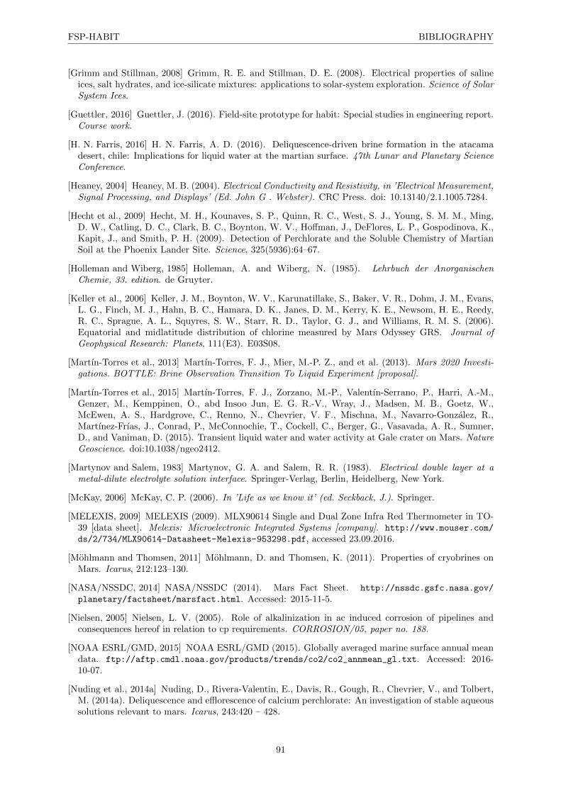
FSP-HABIT BIBLIOGRAPHY
[Grimm and Stillman, 2008] Grimm, R. E. and Stillman, D. E. (2008). Electrical properties of salineices, salt hydrates, and ice-silicate mixtures: applications to solar-system exploration. Science of SolarSystem Ices.
[Guettler, 2016] Guettler, J. (2016). Field-site prototype for habit: Special studies in engineering report.Course work.
[H. N. Farris, 2016] H. N. Farris, A. D. (2016). Deliquescence-driven brine formation in the atacamadesert, chile: Implications for liquid water at the martian surface. 47th Lunar and Planetary ScienceConference.
[Heaney, 2004] Heaney, M. B. (2004). Electrical Conductivity and Resistivity, in ’Electrical Measurement,Signal Processing, and Displays’ (Ed. John G . Webster). CRC Press. doi: 10.13140/2.1.1005.7284.
[Hecht et al., 2009] Hecht, M. H., Kounaves, S. P., Quinn, R. C., West, S. J., Young, S. M. M., Ming,D. W., Catling, D. C., Clark, B. C., Boynton, W. V., Hoffman, J., DeFlores, L. P., Gospodinova, K.,Kapit, J., and Smith, P. H. (2009). Detection of Perchlorate and the Soluble Chemistry of MartianSoil at the Phoenix Lander Site. Science, 325(5936):64–67.
[Holleman and Wiberg, 1985] Holleman, A. and Wiberg, N. (1985). Lehrbuch der AnorganischenChemie, 33. edition. de Gruyter.
[Keller et al., 2006] Keller, J. M., Boynton, W. V., Karunatillake, S., Baker, V. R., Dohm, J. M., Evans,L. G., Finch, M. J., Hahn, B. C., Hamara, D. K., Janes, D. M., Kerry, K. E., Newsom, H. E., Reedy,R. C., Sprague, A. L., Squyres, S. W., Starr, R. D., Taylor, G. J., and Williams, R. M. S. (2006).Equatorial and midlatitude distribution of chlorine measured by Mars Odyssey GRS. Journal ofGeophysical Research: Planets, 111(E3). E03S08.
[Martın-Torres et al., 2013] Martın-Torres, F. J., Mier, M.-P. Z., and et al. (2013). Mars 2020 Investi-gations. BOTTLE: Brine Observation Transition To Liquid Experiment [proposal].
[Martın-Torres et al., 2015] Martın-Torres, F. J., Zorzano, M.-P., Valentın-Serrano, P., Harri, A.-M.,Genzer, M., Kemppinen, O., abd Insoo Jun, E. G. R.-V., Wray, J., Madsen, M. B., Goetz, W.,McEwen, A. S., Hardgrove, C., Renno, N., Chevrier, V. F., Mischna, M., Navarro-Gonzalez, R.,Martınez-Frıas, J., Conrad, P., McConnochie, T., Cockell, C., Berger, G., Vasavada, A. R., Sumner,D., and Vaniman, D. (2015). Transient liquid water and water activity at Gale crater on Mars. NatureGeoscience. doi:10.1038/ngeo2412.
[Martynov and Salem, 1983] Martynov, G. A. and Salem, R. R. (1983). Electrical double layer at ametal-dilute electrolyte solution interface. Springer-Verlag, Berlin, Heidelberg, New York.
[McKay, 2006] McKay, C. P. (2006). In ’Life as we know it’ (ed. Seckback, J.). Springer.
[MELEXIS, 2009] MELEXIS (2009). MLX90614 Single and Dual Zone Infra Red Thermometer in TO-39 [data sheet]. Melexis: Microelectronic Integrated Systems [company]. http://www.mouser.com/
ds/2/734/MLX90614-Datasheet-Melexis-953298.pdf, accessed 23.09.2016.
[Mohlmann and Thomsen, 2011] Mohlmann, D. and Thomsen, K. (2011). Properties of cryobrines onMars. Icarus, 212:123–130.
[NASA/NSSDC, 2014] NASA/NSSDC (2014). Mars Fact Sheet. http://nssdc.gsfc.nasa.gov/
planetary/factsheet/marsfact.html. Accessed: 2015-11-5.
[Nielsen, 2005] Nielsen, L. V. (2005). Role of alkalinization in ac induced corrosion of pipelines andconsequences hereof in relation to cp requirements. CORROSION/05, paper no. 188.
[NOAA ESRL/GMD, 2015] NOAA ESRL/GMD (2015). Globally averaged marine surface annual meandata. ftp://aftp.cmdl.noaa.gov/products/trends/co2/co2_annmean_gl.txt. Accessed: 2016-10-07.
[Nuding et al., 2014a] Nuding, D., Rivera-Valentin, E., Davis, R., Gough, R., Chevrier, V., and Tolbert,M. (2014a). Deliquescence and efflorescence of calcium perchlorate: An investigation of stable aqueoussolutions relevant to mars. Icarus, 243:420 – 428.
91
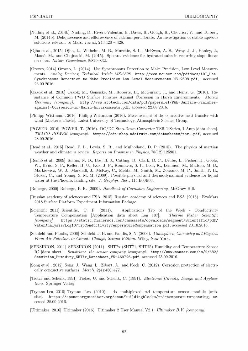
FSP-HABIT BIBLIOGRAPHY
[Nuding et al., 2014b] Nuding, D., Rivera-Valentin, E., Davis, R., Gough, R., Chevrier, V., and Tolbert,M. (2014b). Deliquescence and efflorescence of calcium perchlorate: An investigation of stable aqueoussolutions relevant to Mars. Icarus, 243:420 – 428.
[Ojha et al., 2015] Ojha, L., Wilhelm, M. B., Murchie, S. L., McEwen, A. S., Wray, J. J., Hanley, J.,Masse, M., and Chojnacki, M. (2015). Spectral evidence for hydrated salts in recurring slope lineaeon mars. Nature Geoscience, 8:829–832.
[Orozco, 2014] Orozco, L. (2014). Use Synchronous Detection to Make Precision, Low Level Measure-ments. Analog Devices; Technical Article MS-2698. http://www.mouser.com/pdfdocs/ADI_Use-
Synchronous-Detection-to-Make-Precision-Low-Level-Measurements-MS-2698.pdf, accessed23.09.2016.
[Ozkok et al., 2010] Ozkok, M., Gensicke, M., Roberts, H., McGurran, J., and Heinz, G. (2010). Re-sistance of Common PWB Surface Finishes Against Corrosion in Harsh Environments. AtotechGermany (company). http://www.atotech.com/data/pdf/papers_el/PWB-Surface-Finishes-
against-Corrosion-in-Harsh-Environments.pdf, accessed 22.08.2016.
[Philipp Wittmann, 2016] Philipp Wittmann (2016). Measurement of the convective heat transfer withwind [Master’s Thesis]. Lulea University of Technology, Atmospheric Science Group.
[POWER, 2016] POWER, T. (2016). DC/DC Step-Down Converter TSR 1 Series, 1 Amp [data sheet].TRACO POWER [company]. https://cdn-shop.adafruit.com/datasheets/tsr1.pdf, accessed28.09.2016.
[Read et al., 2015] Read, P. L., Lewis, S. R., and Mulholland, D. P. (2015). The physics of martianweather and climate: a review. Reports on Progress in Physics, 78(12):125901.
[Renno et al., 2009] Renno, N. O., Bos, B. J., Catling, D., Clark, B. C., Drube, L., Fisher, D., Goetz,W., Hviid, S. F., Keller, H. U., Kok, J. F., Kounaves, S. P., Leer, K., Lemmon, M., Madsen, M. B.,Markiewicz, W. J., Marshall, J., McKay, C., Mehta, M., Smith, M., Zorzano, M. P., Smith, P. H.,Stoker, C., and Young, S. M. M. (2009). Possible physical and thermodynamical evidence for liquidwater at the Phoenix landing site. J. Geophys. Res., 115:E00E03.
[Roberge, 2000] Roberge, P. R. (2000). Handbook of Corrosion Engineering. McGraw-Hill.
[Russian academy of sciences and ESA, 2015] Russian academy of sciences and ESA (2015). ExoMars2018 Surface Platform Experiment Information Package.
[Scientific, 2011] Scientific, T. F. (2011). Applications Tip of the Week - ConductivityTemperature Compensation [Application data sheet Log 107]. Thermo Fisher Scientific[company]. https://static.fishersci.com/cmsassets/downloads/segment/Scientific/pdf/
WaterAnalysis/Log107TipConductivityTemperatureCompensation.pdf, accessed 20.10.2016.
[Seinfeld and Pandis, 2006] Seinfeld, J. H. and Pandis, S. N. (2006). Atmospheric Chemistry and Physics:From Air Pollution to Climate Change, Second Edition. Wiley, New York.
[SENSIRION, 2011] SENSIRION (2011). SHT7x (SHT71, SHT75) Humidity and Temperature SensorIC [data sheet]. Sensirion: the sensor company [company]. http://www.mouser.com/ds/2/682/
Sensirion_Humidity_SHT7x_Datasheet_V5-469726.pdf, accessed 23.09.2016.
[Song et al., 2012] Song, J., Wang, L., Zibart, A., and Koch, C. (2012). Corrosion protection of electri-cally conductive surfaces. Metals, 2(4):450–477.
[Tietze and Schenk, 1991] Tietze, U. and Schenk, C. (1991). Electronic Circuits, Design and Applica-tions. Springer Verlag.
[Trystan Lea, 2010] Trystan Lea (2010). 4x multiplexed rtd temperature sensor module [web-site]. https://openenergymonitor.org/emon/buildingblocks/rtd-temperature-sensing, ac-cessed 28.09.2016.
[Ultimaker, 2016] Ultimaker (2016). Ultimaker 2 User Manual V2.1. Ultimaker B.V. [company].
92

FSP-HABIT BIBLIOGRAPHY
[Zent et al., 2009] Zent, A. P., Hecht, M. H., Cobos, D. R., Campbell, G. S., Campbell, C. S., Cardell,G., Foote, M. C., Wood, S. E., and Mehta, M. (2009). Thermal and electrical conductivity probe(tecp) for phoenix. Journal of Geophysical Research: Planets, 114(E3):n/a–n/a. E00A27.
[Zhang, 2010] Zhang, G. (2010). Simulating the electrical double layer capacitance. Excerpt from theProceedings of the COMSOL Conference 2010 Boston. https://www.comsol.com/paper/download/
101189/zhang_paper.pdf.
[Zhang, 2011] Zhang, X. G. (2011). Galvanic Corrsion; In ’Uhlig’s Corrosion Handbook, Third Edition’(ed. R. Winston Revie). John Wiley and Sons, Inc., New York.
[Zorzano et al., 2009] Zorzano, M.-P., Mateo-Martı, E., Prieto-Ballesteros, O., Osuna, S., and Renno,N. (2009). Stability of liquid saline water on present day Mars. Geophys. Res. Lett., 36:L20201.
93
Appendix A
India Campaign: ENVPACK data
A.1 Hunder Dunes, 12.08.2016
0 50 100 150 200 250 300
Time [min]
25
30
35
40
45
50
55
T [
°C]
0
10
20
30
40
50
60
70
80
90
100
RH
[%
]
Temperature data of FSP-HABIT
PressureAGTSA
GTSG
RHA
RHH
0 50 100 150 200 250 300
Time [min]
693.5
694
694.5
695
695.5
696
696.5
697
697.5
698
698.5
p [
hPa
]
Pressure data of FSP-HABIT
PressureP
Figure A.1: ENVPACK data Hunder Dunes.
94
FSP-HABIT APPENDIX A. INDIA CAMPAIGN: ENVPACK DATA
A.2 Kardung La, 13.08.2016
0 5 10 15 20 25 30 35 40 45
Time [min]
0
5
10
15
20
25
30
T [
°C]
0
10
20
30
40
50
60
70
80
90
100
RH
[%
]
Temperature data of FSP-HABIT
PressureAGTSA
GTSG
RHA
RHH
0 5 10 15 20 25 30 35 40 45
Time [min]
541.2
541.3
541.4
541.5
541.6
541.7
541.8
541.9
542
542.1
542.2
p [
hPa
]
Pressure data of FSP-HABIT
PressureP
Figure A.2: ENVPACK data Kardung La
95

FSP-HABIT APPENDIX A. INDIA CAMPAIGN: ENVPACK DATA
A.3 Sundo Lake, 15.08.2016
0 20 40 60 80 100 120 140
Time [min]
0
5
10
15
20
25
30
35
40
T [
°C]
0
10
20
30
40
50
60
70
80
90
100
RH
[%
]
Temperature data of FSP-HABIT
PressureAGTSA
GTSG
RHA
RHH
0 20 40 60 80 100 120 140
Time [min]
574.2
574.4
574.6
574.8
575
575.2
575.4
575.6
575.8
576
576.2
p [
hPa
]
Pressure data of FSP-HABIT
PressureP
Figure A.3: ENVPACK data Sundo Lake
96
FSP-HABIT APPENDIX A. INDIA CAMPAIGN: ENVPACK DATA
A.4 Tso Kar Village, 16.08.2016
0 50 100 150 200 250 300
Time [min]
0
5
10
15
20
25
30
35
40
T [
°C]
0
10
20
30
40
50
60
70
80
90
100
RH
[%
]
Temperature data of FSP-HABIT
PressureAGTSA
GTSG
RHA
RHH
0 50 100 150 200 250 300
Time [min]
582.8
582.9
583
583.1
583.2
583.3
583.4
583.5
583.6
583.7
583.8
p [
hPa
]
Pressure data of FSP-HABIT
PressureP
Figure A.4: ENVPACK data Tso Kar Village
97

FSP-HABIT APPENDIX A. INDIA CAMPAIGN: ENVPACK DATA
A.5 Taglang La, 17.08.2016
0 10 20 30 40 50 60
Time [min]
0
5
10
15
20
25
30
35
40
T [
°C]
0
10
20
30
40
50
60
70
80
90
100
RH
[%
]
Temperature data of FSP-HABIT
PressureAGTSA
GTSG
RHA
RHH
0 10 20 30 40 50 60
Time [min]
536.35
536.4
536.45
536.5
536.55
536.6
536.65
536.7
536.75
536.8
536.85
p [
hPa
]
Pressure data of FSP-HABIT
PressureP
Figure A.5: ENVPACK data Taglang La
98
Appendix B
FSP-HABIT/HOBO DataSide-By-Side
B.1 Relative Humidity
16:00:00 17:00:00 18:00:00 19:00:00 20:00:00
Time [HH:mm:ss]
0
10
20
30
40
50
60
70
80
90
100
RH
[%
]
Iceland RH
HOBORHH
11:00:00 12:00:00 13:00:00 14:00:00 15:00:00 16:00:00 17:00:00
Time [HH:mm:ss]
0
10
20
30
40
50
60
70
80
90
100
RH
[%
]
Hunder Dunes RH
HOBORHH
Figure B.1: Relative humidity data recorded by HOBO and the FSP-HABIT RHS. Iceland and HunderDunes
10:50:00 11:00:00 11:10:00 11:20:00 11:30:00 11:40:00 11:50:00
Time [HH:mm:ss]
0
10
20
30
40
50
60
70
80
90
100
RH
[%
]
Kardung La RH
HOBORHH
10:00:00 10:30:00 11:00:00 11:30:00 12:00:00 12:30:00 13:00:00
Time [HH:mm:ss]
0
10
20
30
40
50
60
70
80
90
100
RH
[%
]
Sundo Lake RH
HOBORHH
Figure B.2: Relative humidity data recorded by HOBO and the FSP-HABIT RHS. Kardung La andSundo Lake
99
FSP-HABIT APPENDIX B. FSP-HABIT/HOBO DATA SIDE-BY-SIDE
14:00:00 15:00:00 16:00:00 17:00:00 18:00:00 19:00:00 20:00:00
Time [HH:mm:ss]
0
10
20
30
40
50
60
70
80
90
100RH
[%
]Tso Kar Village RH
HOBORHH
Figure B.3: Relative humidity data recorded byHOBO and the FSP-HABIT RHS. Tso Kar Village
B.2 Temperatures
16:00:00 17:00:00 18:00:00 19:00:00 20:00:00
Time [HH:mm:ss]
0
5
10
15
20
25
30
35
40
45
50
55
T [
°C]
Iceland Temperatures
HOBOPSA
GTSA
GTSG
RHA
11:00:00 12:00:00 13:00:00 14:00:00 15:00:00 16:00:00 17:00:00
Time [HH:mm:ss]
0
5
10
15
20
25
30
35
40
45
50
55
T [
°C]
Hunder Dunes Temperatures
HOBOPSA
GTSA
GTSG
RHA
Figure B.4: Temperature data recorded by HOBO and the FSP-HABIT RHS. Iceland and Hunder Dunes
10:50:00 11:00:00 11:10:00 11:20:00 11:30:00 11:40:00 11:50:00
Time [HH:mm:ss]
0
5
10
15
20
25
30
35
40
45
50
55
T [
°C]
Kardung La Temperatures
HOBOPSA
GTSA
GTSG
RHA
10:00:00 10:30:00 11:00:00 11:30:00 12:00:00 12:30:00 13:00:00
Time [HH:mm:ss]
0
5
10
15
20
25
30
35
40
45
50
55
T [
°C]
Sundo Lake Temperatures
HOBOPSA
GTSA
GTSG
RHA
Figure B.5: Temperature data recorded by HOBO and the FSP-HABIT RHS. Kardung La and SundoLake
100
FSP-HABIT APPENDIX B. FSP-HABIT/HOBO DATA SIDE-BY-SIDE
14:00:00 15:00:00 16:00:00 17:00:00 18:00:00 19:00:00 20:00:00
Time [HH:mm:ss]
0
5
10
15
20
25
30
35
40
45
50
55T [
°C]
Tso Kar Village Temperatures
HOBOPSA
GTSA
GTSG
RHA
10:15:00 10:30:00 10:45:00 11:00:00 11:15:00 11:30:00
Time [HH:mm:ss]
0
5
10
15
20
25
30
35
40
45
50
55
T [
°C]
Taglang La Temperatures
HOBOPSA
GTSA
GTSG
Figure B.6: Temperature data recorded by HOBO and the FSP-HABIT RHS. Tso Kar Village andTaglang La
101
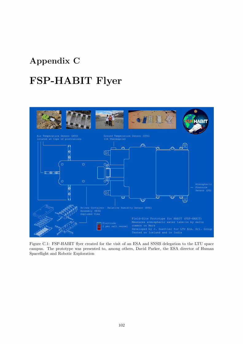
Appendix C
FSP-HABIT Flyer
Ground Temperature Sensor (GTS)(IR Thermopile)
Air Temperature Sensor (ATS)located at tips of protrusions
Relative Humidity Sensor (RHS)
AtmosphericPressureSensor (PS)
Brines ContainerAssembly (BCA)Exploded View
FSPElectrode2 per salt vessel
Field-Site Prototype for HABIT (FSP-HABIT)Measures atmospheric water take-in by saltscommon on MarsDeveloped by J. Guettler for LTU Atm. Sci. GroupTested on Iceland and in India
Figure C.1: FSP-HABIT flyer created for the visit of an ESA and SNSB delegation to the LTU spacecampus. The prototype was presented to, among others, David Parker, the ESA director of HumanSpaceflight and Robotic Exploration
102

Appendix D
FSP-HABIT Code
1 #inc lude <Wire . h>2 #inc lude <SD. h>3 #inc lude <SPI . h>4 #inc lude <Adafruit MLX90614 . h>5 #inc lude <Adaf ru i t Senso r . h>6 #inc lude <Adafruit BMP085 U . h>7 #inc lude <S e n s i r i o n . h>8 extern ”C” 9 #inc lude ” u t i l i t y / twi . h” // from Wire l i b r a r y , so we can do bus scanning
10 11 // Def ine po in t e r f o r SD sav ing12 F i l e myFile ;13
14 Adafruit MLX90614 mlx = Adafruit MLX90614 ( ) ;15 Adafruit BMP085 Unif ied bmp = Adafruit BMP085 Unif ied (10085) ;16
17 // Sensor parameters18 const u i n t 8 t dataPin = 9 ; // SHT s e r i a l data19 const u i n t 8 t s c lkP in = 8 ; // SHT s e r i a l c l o ck20 // const u i n t 8 t ledPin = 13 ; // Arduino bu i l t - in LED21 const u i n t 3 2 t TRHSTEP = 5000UL; // Rh Sensor query per iod22 const u i n t 3 2 t SENSORSTEP = 1000UL; // Environmental s enso r query per iod23 const u i n t 3 2 t CONDSTEP = 500UL; // AC Conduct iv i ty s enso r query per iod24
25 S e n s i r i o n sht = S e n s i r i o n ( dataPin , s c lkP in ) ;26
27 u i n t 1 6 t rawData ;28 f l o a t temperature ;29 f l o a t humidity ;30 f l o a t dewpoint ;31
32 // byte l edS ta t e = 0 ;33 byte measActive = f a l s e ;34 byte measType = TEMP;35
36 unsigned long t r h M i l l i s = 0 ; // Time i n t e r v a l t r a ck ing37 unsigned long s e n s o r M i l l i s = 0 ;38 unsigned long condM i l l i s = 0 ;39
40 //ATS 1 2 341 i n t ATS1 = A1 ;42 i n t ATS2 = A2 ;43 i n t ATS3 = A3 ;44
45 double A = 3.9083*pow(10 , - 3 ) ;46 double B = -5 .7750*pow(10 , - 7 ) ;47 double C = -4 .1830*pow(10 , -12 ) ;48
49 // S e l e c t chip f o r SD reader50 const i n t c h i p S e l e c t = 53 ;51
52 i n t d ig1 = 3 ; //PWM 153 i n t d ig2 = 5 ; //PWM 2
103
FSP-HABIT APPENDIX D. FSP-HABIT CODE
54 i n t an1 = A4 ; // read vo l tage f o r conduc t i v i t y e s t imat i on55 i n t b lock = 1 ; // Block ATS from swi tch ing to 1 .1 V r e f e r e n c e vo l tage when measuring56 conduc t i v i ty57
58 // Var i ab l e s f o r analog read59 i n t a100 ;60 i n t a1k ;61 i n t a10k ;62 i n t a100k ;63 i n t a1M;64 i n t a4M;65
66 i n t counte r sw i t ch = 1 ; // counter to switch between measurement po in t s67 i n t c o u n t e r r e f = 1 ; // counter f o r sw i t ch ing r e f e r e n c e r e s i s t o r s , NOT us ing 4M due to68 p o s s i b l e d i s connec t69 double counter = 0 ; // counter f o r measuring V only every X step70 double rx ; // r e s i s t a n c e71 double rx4M ;72 double rx1M ;73 double rx100k ;74 double rx10k ;75 double rx1k ;76 double rx100 ;77
78 double vcond ; // vo l tage conduc t i v i ty probe79 double vca l c ; // vo l tage f o r c a l l i b r a t i o n / c a l c u l a t i o n80 double v100 = 6 ;81 double v1k = 6 ;82 double v10k = 6 ;83 double v100k = 6 ;84 double v1M = 6 ;85 double v4M = 6 ;86 double i ;87
88 // Reference R e s i s t o r Switching89 i n t r e f 1 = 22 ; //Check Pins !90 i n t r e f 2 = 23 ;91 i n t r e f 3 = 24 ;92 i n t r e f 4 = 25 ;93 i n t r e f 5 = 26 ;94 i n t r e f 6 = 27 ;95
96 //Measurement Points Switching97 i n t cur r ent = 0 ; // which switch to turn on98
99 i n t v1 1 = 28 ; // I n s e r t Pin numbers100 i n t v1 2 = 29 ;101 i n t v1 3 = 30 ;102
103 i n t v2 1 = 31 ;104 i n t v2 2 = 32 ;105 i n t v2 3 = 33 ;106
107 i n t v3 1 = 34 ;108 i n t v3 2 = 35 ;109 i n t v3 3 = 36 ;110
111 i n t v4 1 = 37 ;112 i n t v4 2 = 38 ;113 i n t v4 3 = 39 ;114
115 i n t v5 1 = 40 ;116 i n t v5 2 = 41 ;117 i n t v5 3 = 42 ;118
119 i n t v6 1 = 43 ;120 i n t v6 2 = 44 ;121 i n t v6 3 = 45 ;122
123 void setup ( )124 125 // Open s e r i a l communications and wait f o r port to open :126 S e r i a l . begin (38400) ;
104
FSP-HABIT APPENDIX D. FSP-HABIT CODE
127 whi le ( ! S e r i a l ) 128 ; // wait f o r s e r i a l port to connect .129 130
131
132 S e r i a l . p r i n t ( ” I n i t i a l i z i n g SD card . . . ” ) ;133 // make sure that the d e f a u l t chip s e l e c t pin i s s e t to134 // output , even i f you don ' t use i t :135 // pinMode (53 , OUTPUT) ; //Why was t h i s not needed ??136
137 // see i f the card i s pre sent and can be i n i t i a l i z e d :138 i f ( ! SD. begin ( c h i p S e l e c t ) ) 139 S e r i a l . p r i n t l n ( ”Card f a i l e d , or not pre sent ” ) ;140 // don ' t do anything more :141 r e turn ;142 143 S e r i a l . p r i n t l n ( ” card i n i t i a l i z e d . ” ) ;144
145 Wire . begin ( ) ;146
147 // Pressure148 /* I n i t i a l i s e the s enso r */149 bmp. begin ( ) ;150
151 // GTS152 // S e r i a l . p r i n t l n (”FSP-HABIT MLX90614 GTS”) ;153 mlx . begin ( ) ;154
155 // CONDUCTIVITY MEASUREMENT SET-UP156 pinMode ( dig1 , OUTPUT) ;157 pinMode ( dig2 , OUTPUT) ;158
159 // Reference r e s i s t o r switch160 pinMode ( re f1 , OUTPUT) ;161 pinMode ( re f2 , OUTPUT) ;162 pinMode ( re f3 , OUTPUT) ;163 pinMode ( re f4 , OUTPUT) ;164 pinMode ( re f5 , OUTPUT) ;165 pinMode ( re f6 , OUTPUT) ;166
167
168 d i g i t a l W r i t e ( dig1 , LOW) ;169 d i g i t a l W r i t e ( dig2 , LOW) ;170
171 // Reference , a l l o f f at i n i t i a l i z a t i o n except h i ghe s t172 d i g i t a l W r i t e ( r e f1 , LOW) ; // 100 Ohm173 d i g i t a l W r i t e ( r e f2 , LOW) ; // 1k174 d i g i t a l W r i t e ( r e f3 , LOW) ; // 10k175 d i g i t a l W r i t e ( r e f4 , LOW) ; // 100k176 d i g i t a l W r i t e ( r e f5 , LOW) ; // 1M, because o f p o s s i b l e 4M di s connec t177 d i g i t a l W r i t e ( r e f6 , HIGH) ; // 4M178
179 pinMode ( an1 , INPUT) ;180
181 // Switches182 pinMode ( v1 1 , OUTPUT) ; //1183 pinMode ( v1 2 , OUTPUT) ; //2184 pinMode ( v1 3 , OUTPUT) ; //3185
186 pinMode ( v2 1 , OUTPUT) ; //4187 pinMode ( v2 2 , OUTPUT) ; //5188 pinMode ( v2 3 , OUTPUT) ; //6189
190 pinMode ( v3 1 , OUTPUT) ; //7191 pinMode ( v3 2 , OUTPUT) ; //8192 pinMode ( v3 3 , OUTPUT) ; //9193
194 pinMode ( v4 1 , OUTPUT) ; //10195 pinMode ( v4 2 , OUTPUT) ; //11196 pinMode ( v4 3 , OUTPUT) ; //12197
198 pinMode ( v5 1 , OUTPUT) ; //13199 pinMode ( v5 2 , OUTPUT) ; //14
105
FSP-HABIT APPENDIX D. FSP-HABIT CODE
200 pinMode ( v5 3 , OUTPUT) ; //15201
202 pinMode ( v6 1 , OUTPUT) ; //16203 pinMode ( v6 2 , OUTPUT) ; //17204 pinMode ( v6 3 , OUTPUT) ; //18205
206 // Set a l l sw i t che s to block i n i t i a l l y207 d i g i t a l W r i t e ( v1 1 , LOW) ;208 d i g i t a l W r i t e ( v1 2 , LOW) ;209 d i g i t a l W r i t e ( v1 3 , LOW) ;210
211 d i g i t a l W r i t e ( v2 1 , LOW) ;212 d i g i t a l W r i t e ( v2 2 , LOW) ;213 d i g i t a l W r i t e ( v2 3 , LOW) ;214
215 d i g i t a l W r i t e ( v3 1 , LOW) ;216 d i g i t a l W r i t e ( v3 2 , LOW) ;217 d i g i t a l W r i t e ( v3 3 , LOW) ;218
219 d i g i t a l W r i t e ( v4 1 , LOW) ;220 d i g i t a l W r i t e ( v4 2 , LOW) ;221 d i g i t a l W r i t e ( v4 3 , LOW) ;222
223 d i g i t a l W r i t e ( v5 1 , LOW) ;224 d i g i t a l W r i t e ( v5 2 , LOW) ;225 d i g i t a l W r i t e ( v5 3 , LOW) ;226
227 d i g i t a l W r i t e ( v6 1 , LOW) ;228 d i g i t a l W r i t e ( v6 2 , LOW) ;229 d i g i t a l W r i t e ( v6 3 , LOW) ;230
231 ana logReference (EXTERNAL) ;232
233 // Write header on f i l e234 myFile = SD. open ( ”FSP . txt ” , FILE WRITE) ;235
236 i f ( myFile ) 237 myFile . p r i n t l n ( ”” ) ;238 myFile . p r i n t l n ( ”New Measurement s t a r t e d ” ) ;239 myFile . p r i n t l n ( ”Time \ t Ves se l \ t V 1M \ t R 1M \ t V 100k \ t R 100k \ t V 10k \ t R 10k240 \ t V 1k \ t R 1k \ t V 100 \ t R 100 \ t Pressure T \ t Pres sure p \ t GTS Ambient T241 \ t GTS Ground T \ t RH T \ t RH RH \ t RH Dewpoint” ) ;242 // c l o s e the f i l e : 000243 myFile . c l o s e ( ) ;244 245
246 cur rent = v1 1 ;247 switchReg ( ) ;248
249 250
251
252 void loop ( ) 253
254 // Create AC square wave :255 d i g i t a l W r i t e ( dig1 , HIGH) ;256 d i g i t a l W r i t e ( dig2 , LOW) ;257 delayMicroseconds (484) ; //1kHz258
259 d i g i t a l W r i t e ( dig1 , LOW) ;260 d i g i t a l W r i t e ( dig2 , HIGH) ;261 delayMicroseconds (460) ; //1kHz262
263 // Get cur rent time264 unsigned long c u r M i l l i s = m i l l i s ( ) ;265
266 counter++;267
268 i f ( counter == 675) 269 // Block ATS from swi tch ing to 1 .1V270 block = 1 ;271
272 // Switch between measurement po in t s
106

FSP-HABIT APPENDIX D. FSP-HABIT CODE
273 i f ( counte r sw i t ch == 1) 274 cur rent = v1 1 ;275
276 i f ( counte r sw i t ch == 2) 277 cur rent = v1 2 ;278
279 i f ( counte r sw i t ch == 3) 280 cur rent = v1 3 ;281
282 i f ( counte r sw i t ch == 4) 283 cur rent = v2 1 ;284
285 i f ( counte r sw i t ch == 5) 286 cur rent = v2 2 ;287
288 i f ( counte r sw i t ch == 6) 289 cur rent = v2 3 ;290
291 i f ( counte r sw i t ch == 7) 292 cur rent = v3 1 ;293
294 i f ( counte r sw i t ch == 8) 295 cur rent = v3 2 ;296
297 i f ( counte r sw i t ch == 9) 298 cur rent = v3 3 ;299
300 i f ( counte r sw i t ch == 10) 301 cur rent = v4 1 ;302
303 i f ( counte r sw i t ch == 11) 304 cur rent = v4 2 ;305
306 i f ( counte r sw i t ch == 12) 307 cur rent = v4 3 ;308
309 i f ( counte r sw i t ch == 13) 310 cur rent = v5 1 ;311
312 i f ( counte r sw i t ch == 14) 313 cur rent = v5 2 ;314
315 i f ( counte r sw i t ch == 15) 316 cur rent = v5 3 ;317
318 i f ( counte r sw i t ch == 16) 319 cur rent = v6 1 ;320
321 i f ( counte r sw i t ch == 17) 322 cur rent = v6 2 ;323
324 i f ( counte r sw i t ch == 18) 325 cur rent = v6 3 ;326
327 i f ( c o u n t e r r e f == 1)328 329 switchReg ( ) ;330
331 delayMicroseconds (5000) ;332 a4M = analogRead ( an1 ) ; // read senso r va lue f o r cond333
334 v4M = a4M * 0 . 00322 ;335 rx4M = 4000 * 4 .70 / v4M - 1000 ;336
337 S e r i a l . p r i n t ( ”V 4M = ” ) ;338 S e r i a l . p r i n t (v4M) ;339 S e r i a l . p r i n t ( ” ; R 4M = ” ) ;340 S e r i a l . p r i n t (rx4M) ;341 S e r i a l . p r i n t l n ( ” kOhm” ) ;342
343 // Prepare next measurement344 d i g i t a l W r i t e ( r e f1 , LOW) ; // 100345 d i g i t a l W r i t e ( r e f2 , LOW) ; // 1k
107
FSP-HABIT APPENDIX D. FSP-HABIT CODE
346 d i g i t a l W r i t e ( r e f3 , LOW) ; // 10k347 d i g i t a l W r i t e ( r e f4 , LOW) ; // 100k348 d i g i t a l W r i t e ( r e f5 , HIGH) ; // 1M349 d i g i t a l W r i t e ( r e f6 , LOW) ; // 4M350
351 352
353 i f ( c o u n t e r r e f == 2)354 355 // switchReg ( ) ;356
357 delayMicroseconds (5000) ;358 a1M = analogRead ( an1 ) ; // read senso r va lue f o r cond359
360 v1M = a1M * 0 . 00322 ;361 rx1M = 1000 * 4 .70 / v1M - 1000 ;362
363 S e r i a l . p r i n t ( ”V 1M = ” ) ;364 S e r i a l . p r i n t (v1M) ;365 S e r i a l . p r i n t ( ” ; R 1M = ” ) ;366 S e r i a l . p r i n t (rx1M) ;367 S e r i a l . p r i n t l n ( ” kOhm” ) ;368
369 // Prepare next measurement370 d i g i t a l W r i t e ( r e f1 , LOW) ; // 100371 d i g i t a l W r i t e ( r e f2 , LOW) ; // 1k372 d i g i t a l W r i t e ( r e f3 , LOW) ; // 10k373 d i g i t a l W r i t e ( r e f4 , HIGH) ; // 100k374 d i g i t a l W r i t e ( r e f5 , LOW) ; // 1M375 d i g i t a l W r i t e ( r e f6 , LOW) ; // 4M376
377 378
379 i f ( c o u n t e r r e f == 3)380 381 delayMicroseconds (500) ;382 a100k = analogRead ( an1 ) ; // read senso r va lue f o r cond383
384 v100k = a100k * 0 . 00322 ;385 rx100k = 100 * 4 .70 / v100k - 100 ;386
387 S e r i a l . p r i n t ( ”V 100k = ” ) ;388 S e r i a l . p r i n t ( v100k ) ;389 S e r i a l . p r i n t ( ” ; R 100k = ” ) ;390 S e r i a l . p r i n t ( rx100k ) ;391 S e r i a l . p r i n t l n ( ” kOhm” ) ;392
393 // Prepare next measurement394 d i g i t a l W r i t e ( r e f1 , LOW) ; // 100395 d i g i t a l W r i t e ( r e f2 , LOW) ; // 1k396 d i g i t a l W r i t e ( r e f3 , HIGH) ; // 10k397 d i g i t a l W r i t e ( r e f4 , LOW) ; // 100k398 d i g i t a l W r i t e ( r e f5 , LOW) ; // 1M399 d i g i t a l W r i t e ( r e f6 , LOW) ; // 4M400 401 i f ( c o u n t e r r e f == 4)402 403 a10k = analogRead ( an1 ) ; // read senso r va lue f o r cond404
405 v10k = a10k * 0 . 00322 ;406 rx10k = 10 * 4 .70 / v10k - 10 ;407
408 S e r i a l . p r i n t ( ”V 10k = ” ) ;409 S e r i a l . p r i n t ( v10k ) ;410 S e r i a l . p r i n t ( ” ; R 10k = ” ) ;411 S e r i a l . p r i n t ( rx10k ) ;412 S e r i a l . p r i n t l n ( ” kOhm” ) ;413
414 // Prepare next measurement415 d i g i t a l W r i t e ( r e f1 , LOW) ; // 100416 d i g i t a l W r i t e ( r e f2 , HIGH) ; // 1k417 d i g i t a l W r i t e ( r e f3 , LOW) ; // 10k418 d i g i t a l W r i t e ( r e f4 , LOW) ; // 100k
108

FSP-HABIT APPENDIX D. FSP-HABIT CODE
419 d i g i t a l W r i t e ( r e f5 , LOW) ; // 1M420 d i g i t a l W r i t e ( r e f6 , LOW) ; // 4M421 422 i f ( c o u n t e r r e f == 5)423 424 a1k = analogRead ( an1 ) ; // read senso r va lue f o r cond425
426 v1k = a1k * 0 . 00322 ;427 rx1k = 1 * 4 .70 / v1k - 1 ;428
429 S e r i a l . p r i n t ( ”V 1k = ” ) ;430 S e r i a l . p r i n t ( v1k ) ;431 S e r i a l . p r i n t ( ” ; R 1k = ” ) ;432 S e r i a l . p r i n t ( rx1k ) ;433 S e r i a l . p r i n t l n ( ” kOhm” ) ;434
435 // Prepare next measurement436 d i g i t a l W r i t e ( r e f1 , HIGH) ; // 100437 d i g i t a l W r i t e ( r e f2 , LOW) ; // 1k438 d i g i t a l W r i t e ( r e f3 , LOW) ; // 10k439 d i g i t a l W r i t e ( r e f4 , LOW) ; // 100k440 d i g i t a l W r i t e ( r e f5 , LOW) ; // 1M441 d i g i t a l W r i t e ( r e f6 , LOW) ; // 4M442 443
444 i f ( c o u n t e r r e f == 6)445 446 a100 = analogRead ( an1 ) ; // read senso r va lue f o r cond447
448 v100 = a100 * 0 . 00322 ;449 rx100 = 100 * 4 .70 / v100 - 100 ;450
451 S e r i a l . p r i n t ( ”V 100 = ” ) ;452 S e r i a l . p r i n t ( v100 ) ;453 S e r i a l . p r i n t ( ” ; R 100 = ” ) ;454 S e r i a l . p r i n t ( rx100 ) ;455 S e r i a l . p r i n t l n ( ” Ohm” ) ;456
457 // Prepare next measurement458 d i g i t a l W r i t e ( r e f1 , LOW) ; // 100459 d i g i t a l W r i t e ( r e f2 , LOW) ; // 1k460 d i g i t a l W r i t e ( r e f3 , LOW) ; // 10k461 d i g i t a l W r i t e ( r e f4 , LOW) ; // 100k462 d i g i t a l W r i t e ( r e f5 , LOW) ; // 1M //NOT using 4M due to p o s s i b l e d i s connec t463 d i g i t a l W r i t e ( r e f6 , HIGH) ; // 4M464 465
466 counter = 0 ;467 c o u n t e r r e f ++;468 i f ( c o u n t e r r e f == 7)469 470 //New l i n e in f i l e f o r cond measurement471 //Format : Time | Vesse l | r e f 1 | r e f 2 | r e f 3 | . . .472 myFile = SD. open ( ”FSP . txt ” , FILE WRITE) ;473
474 i f ( myFile ) 475 myFile . p r i n t l n ( ”” ) ;476 myFile . p r i n t ( c u r M i l l i s ) ;477 myFile . p r i n t ( ”\ t ” ) ;478
479 // Switch between measurement po in t s480 i f ( counte r sw i t ch == 1) 481 myFile . p r i n t ( ”V1 1\ t ” ) ;482
483 i f ( counte r sw i t ch == 2) 484 myFile . p r i n t ( ”V1 2\ t ” ) ;485
486 i f ( counte r sw i t ch == 3) 487 myFile . p r i n t ( ”V1 3\ t ” ) ;488
489 i f ( counte r sw i t ch == 4) 490 myFile . p r i n t ( ”V2 1\ t ” ) ;491
109
FSP-HABIT APPENDIX D. FSP-HABIT CODE
492 i f ( counte r sw i t ch == 5) 493 myFile . p r i n t ( ”V2 2\ t ” ) ;494
495 i f ( counte r sw i t ch == 6) 496 myFile . p r i n t ( ”V2 3\ t ” ) ;497
498 i f ( counte r sw i t ch == 7) 499 myFile . p r i n t ( ”V3 1\ t ” ) ;500
501 i f ( counte r sw i t ch == 8) 502 myFile . p r i n t ( ”V3 2\ t ” ) ;503
504 i f ( counte r sw i t ch == 9) 505 myFile . p r i n t ( ”V3 3\ t ” ) ;506
507 i f ( counte r sw i t ch == 10) 508 myFile . p r i n t ( ”V4 1\ t ” ) ;509
510 i f ( counte r sw i t ch == 11) 511 myFile . p r i n t ( ”V4 2\ t ” ) ;512
513 i f ( counte r sw i t ch == 12) 514 myFile . p r i n t ( ”V4 3\ t ” ) ;515
516 i f ( counte r sw i t ch == 13) 517 myFile . p r i n t ( ”V5 1\ t ” ) ;518
519 i f ( counte r sw i t ch == 14) 520 myFile . p r i n t ( ”V5 2\ t ” ) ;521
522 i f ( counte r sw i t ch == 15) 523 myFile . p r i n t ( ”V5 3\ t ” ) ;524
525 i f ( counte r sw i t ch == 16) 526 myFile . p r i n t ( ”V6 1\ t ” ) ;527
528 i f ( counte r sw i t ch == 17) 529 myFile . p r i n t ( ”V6 2\ t ” ) ;530
531 i f ( counte r sw i t ch == 18) 532 myFile . p r i n t ( ”V6 3\ t ” ) ;533
534 // myFile . p r i n t (v4M) ;535 // myFile . p r i n t (”\ t ”) ;536 // myFile . p r i n t (rx4M) ;537 // myFile . p r i n t (” kOhm\ t ”) ;538
539 myFile . p r i n t (v1M) ;540 myFile . p r i n t ( ”\ t ” ) ;541 myFile . p r i n t ( rx1M) ;542 myFile . p r i n t ( ” kOhm\ t ” ) ;543
544 myFile . p r i n t ( v100k ) ;545 myFile . p r i n t ( ”\ t ” ) ;546 myFile . p r i n t ( rx100k ) ;547 myFile . p r i n t ( ” kOhm\ t ” ) ;548
549 myFile . p r i n t ( v10k ) ;550 myFile . p r i n t ( ”\ t ” ) ;551 myFile . p r i n t ( rx10k ) ;552 myFile . p r i n t ( ” kOhm\ t ” ) ;553
554 myFile . p r i n t ( v1k ) ;555 myFile . p r i n t ( ”\ t ” ) ;556 myFile . p r i n t ( rx1k ) ;557 myFile . p r i n t ( ” kOhm\ t ” ) ;558
559 myFile . p r i n t ( v100 ) ;560 myFile . p r i n t ( ”\ t ” ) ;561 myFile . p r i n t ( rx100 ) ;562 myFile . p r i n t ( ” Ohm\ t ” ) ;563
564 // Pressure
110
FSP-HABIT APPENDIX D. FSP-HABIT CODE
565 /* Get a new senso r event */566 s e n s o r s e v e n t t event ;567 bmp. getEvent(&event ) ;568
569 /* Display the r e s u l t s ( barometr ic p r e s su r e i s measure in hPa) */570 i f ( event . p r e s su r e )571 572 /* get the cur rent temperature from the BMP085 */573 f l o a t temperature ;574 bmp. getTemperature(&temperature ) ;575
576 myFile . p r i n t ( temperature ) ;577 myFile . p r i n t ( ” C\ t ” ) ;578 myFile . p r i n t ( event . p r e s su r e ) ;579 myFile . p r i n t ( ” hPa\ t ” ) ;580 581
582 myFile . p r i n t ( mlx . readAmbientTempC ( ) ) ;583 myFile . p r i n t ( ” C\ t ” ) ; myFile . p r i n t ( mlx . readObjectTempC ( ) ) ; myFile . p r i n t ( ” C\ t ” ) ;584
585 // c l o s e the f i l e : 000586 myFile . c l o s e ( ) ;587 588
589 c o u n t e r r e f = 1 ; //NOT us ing 4M due to p o s s i b l e d i s connec t590 counte r sw i t ch++;591
592 i f ( counte r sw i t ch == 19)593 594 counte r sw i t ch = 1 ;595 myFile = SD. open ( ”FSP . txt ” , FILE WRITE) ;596
597 S e r i a l . p r i n t l n ( ”” ) ;598 599 // block = 0 ; // r e l e a s e600
601 // c l o s e the f i l e :602 // myFile . c l o s e ( ) ;603 //604 605
606 // RH sensor , non - b lock ing c a l l607 i f ( c u r M i l l i s - t r h M i l l i s >= TRHSTEP) // Time f o r new measurements ?608 measActive = true ;609 measType = TEMP;610 sht . meas (TEMP, &rawData , NONBLOCK) ; // Star t temp measurement611 t r h M i l l i s = c u r M i l l i s ;612 613 i f ( measActive && sht . measRdy ( ) ) // Note : no e r r o r check ing614 i f ( measType == TEMP) // Process temp or humi?615 measType = HUMI;616 temperature = sht . calcTemp ( rawData ) ; // Convert raw senso r data617 sht . meas (HUMI, &rawData , NONBLOCK) ; // Star t humidity measurement618 e l s e 619 measActive = f a l s e ;620 humidity = sht . calcHumi ( rawData , temperature ) ; // Convert raw senso r data621 dewpoint = sht . calcDewpoint ( humidity , temperature ) ;622 logDataRH ( ) ;623 624 625 626
627 void logDataRH ( ) 628 S e r i a l . p r i n t ( ”Temperature = ” ) ; S e r i a l . p r i n t ( temperature ) ;629 S e r i a l . p r i n t ( ” C, Humidity = ” ) ; S e r i a l . p r i n t ( humidity ) ;630 S e r i a l . p r i n t ( ” %, Dewpoint = ” ) ; S e r i a l . p r i n t ( dewpoint ) ;631 S e r i a l . p r i n t l n ( ” C” ) ;632 myFile = SD. open ( ”FSP . txt ” , FILE WRITE) ;633
634 i f ( myFile ) 635 myFile . p r i n t ( temperature ) ;636 myFile . p r i n t ( ” C\ t ” ) ;637 myFile . p r i n t ( humidity ) ;
111

FSP-HABIT APPENDIX D. FSP-HABIT CODE
638 myFile . p r i n t ( ” %\t ” ) ;639 myFile . p r i n t ( dewpoint ) ;640 myFile . p r i n t ( ” C\ t ” ) ;641 // c l o s e the f i l e :642 myFile . c l o s e ( ) ;643 644
645 646
647 void switchReg ( ) 648 d i g i t a l W r i t e ( v1 1 , LOW) ;649 d i g i t a l W r i t e ( v1 2 , LOW) ;650 d i g i t a l W r i t e ( v1 3 , LOW) ;651
652 d i g i t a l W r i t e ( v2 1 , LOW) ;653 d i g i t a l W r i t e ( v2 2 , LOW) ;654 d i g i t a l W r i t e ( v2 3 , LOW) ;655
656 d i g i t a l W r i t e ( v3 1 , LOW) ;657 d i g i t a l W r i t e ( v3 2 , LOW) ;658 d i g i t a l W r i t e ( v3 3 , LOW) ;659
660 d i g i t a l W r i t e ( v4 1 , LOW) ;661 d i g i t a l W r i t e ( v4 2 , LOW) ;662 d i g i t a l W r i t e ( v4 3 , LOW) ;663
664 d i g i t a l W r i t e ( v5 1 , LOW) ;665 d i g i t a l W r i t e ( v5 2 , LOW) ;666 d i g i t a l W r i t e ( v5 3 , LOW) ;667
668 d i g i t a l W r i t e ( v6 1 , LOW) ;669 d i g i t a l W r i t e ( v6 2 , LOW) ;670 d i g i t a l W r i t e ( v6 3 , LOW) ;671
672 d i g i t a l W r i t e ( current , HIGH) ;673
112
Related Documents