Field Evaluation of Built-In Curling Levels in Rigid Pavements Jacob Hiller, Principal Investigator Michigan Technological University June 2011 Research Project Final Report 2011-16

Welcome message from author
This document is posted to help you gain knowledge. Please leave a comment to let me know what you think about it! Share it to your friends and learn new things together.
Transcript

Field Evaluation of Built-InCurling Levels in Rigid Pavements
Jacob Hiller, Principal InvestigatorMichigan Technological University
June 2011Research Project
Final Report 2011-16

All agencies, departments, divisions and units that develop, use and/or purchase written materials for distribution to the public must ensure that each document contain a statement indicating that the information is available in alternative formats to individuals with disabilities upon request. Include the following statement on each document that is distributed: To request this document in an alternative format, call Bruce Lattu at 651-366-4718 or 1-800-657-3774 (Greater Minnesota); 711 or 1-800-627-3529 (Minnesota Relay). You may also send an e-mail to [email protected]. (Please request at least one week in advance).
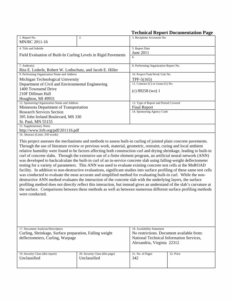
Technical Report Documentation Page 1. Report No. 2. 3. Recipients Accession No. MN/RC 2011-16
4. Title and Subtitle 5. Report Date
Field Evaluation of Built-In Curling Levels in Rigid Pavements June 2011 6.
7. Author(s) 8. Performing Organization Report No. Rita E. Lederle, Robert W. Lothschutz, and Jacob E. Hiller 9. Performing Organization Name and Address 10. Project/Task/Work Unit No. Michigan Technological University Department of Civil and Environmental Engineering 1400 Townsend Drive 210F Dillman Hall Houghton, MI 49931
TPF-5(165) 11. Contract (C) or Grant (G) No.
(c) 89258 (wo) 1
12. Sponsoring Organization Name and Address 13. Type of Report and Period Covered Minnesota Department of Transportation Research Services Section 395 John Ireland Boulevard, MS 330 St. Paul, MN 55155
Final Report 14. Sponsoring Agency Code
15. Supplementary Notes http://www.lrrb.org/pdf/201116.pdf 16. Abstract (Limit: 250 words)
This project assesses the mechanisms and methods to assess built-in curling of jointed plain concrete pavements. Through the use of literature review or previous work, material, geometric, restraint, curing and local ambient relative humidity were found to be factors affecting both construction curl and drying shrinkage, leading to built-in curl of concrete slabs. Through the extensive use of a finite element program, an artificial neural network (ANN) was developed to backcalculate the built-in curl of an in-service concrete slab using falling-weight deflectometer testing for a variety of parameters. This ANN was used to evaluate existing concrete test cells at the MnROAD facility. In addition to non-destructive evaluations, significant studies into surface profiling of these same test cells was conducted to evaluate the most accurate and simplified method for evaluating built-in curl. While the non-destructive ANN method evaluates the interaction of the concrete slab with the underlying layers, the surface profiling method does not directly reflect this interaction, but instead gives an understand of the slab’s curvature at the surface. Comparisons between these methods as well as between numerous different surface profiling methods were conducted.
17. Document Analysis/Descriptors 18. Availability Statement Curling, Shrinkage, Surface preparation, Falling weight deflectometers, Curling, Warpage
No restrictions. Document available from: National Technical Information Services, Alexandria, Virginia 22312
19. Security Class (this report) 20. Security Class (this page) 21. No. of Pages 22. Price Unclassified Unclassified 342
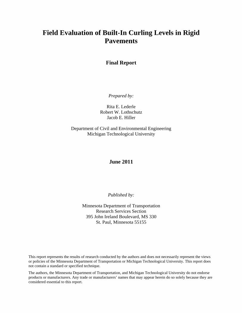
Field Evaluation of Built-In Curling Levels in Rigid Pavements
Final Report
Prepared by:
Rita E. Lederle Robert W. Lothschutz
Jacob E. Hiller
Department of Civil and Environmental Engineering Michigan Technological University
June 2011
Published by:
Minnesota Department of Transportation Research Services Section
395 John Ireland Boulevard, MS 330 St. Paul, Minnesota 55155
This report represents the results of research conducted by the authors and does not necessarily represent the views or policies of the Minnesota Department of Transportation or Michigan Technological University. This report does not contain a standard or specified technique.
The authors, the Minnesota Department of Transportation, and Michigan Technological University do not endorse products or manufacturers. Any trade or manufacturers’ names that may appear herein do so solely because they are considered essential to this report.

TABLE OF CONTENTS
INTRODUCTION .......................................................................................................................... 1 TASK 1: LITERATURE REVIEW ................................................................................................ 2
Mechanics of curling and warping .............................................................................................. 2 Temperature gradient .............................................................................................................. 2 Moisture gradient .................................................................................................................... 3 Built-in temperature gradient .................................................................................................. 4 Differential drying shrinkage .................................................................................................. 4 Creep ....................................................................................................................................... 5
Geometric and material properties .............................................................................................. 6 Concrete material properties ................................................................................................... 6 Slab geometry ......................................................................................................................... 6 Slab thickness.......................................................................................................................... 7 Joint restraint mechanisms ...................................................................................................... 7 Subgrade characteristics.......................................................................................................... 8
Effect of curling on fatigue cracking type .................................................................................. 9 Factors that affect built-in curling ............................................................................................. 11
Paving season ........................................................................................................................ 11 Paving time ........................................................................................................................... 12 Curing techniques ................................................................................................................. 12 Mix design ............................................................................................................................ 13
Analysis and modeling of curling and warping ........................................................................ 13 Historical approaches ............................................................................................................ 14 Back-calculation methods ..................................................................................................... 14
Methods of collecting field data ............................................................................................... 16 Dipstick Auto-Read Profiler ................................................................................................. 16 Falling weight deflectometer ................................................................................................ 16 MnROAD testing facility ...................................................................................................... 17
Overview of specific site studies .............................................................................................. 17 Florida DOT test road ........................................................................................................... 17 Chilean PCC in-service test road network ............................................................................ 18 Arizona and Minnesota field tests......................................................................................... 18 Michigan freeway pavement tests ......................................................................................... 19 Pennsylvania test section ...................................................................................................... 19 Summary of specific site studies........................................................................................... 20
TASK 2: DEVELOPMENT OF FWD BACKCALCULATION ALGORITHM FOR BUILT-IN CURL DETERMINATION .......................................................................................................... 21
Selection of modeling parameters ............................................................................................. 21 Dimensional analysis ............................................................................................................ 21 Geometric variables .............................................................................................................. 23 Material properties ................................................................................................................ 27 FWD layout ........................................................................................................................... 27 Other parameters ................................................................................................................... 28
Modeling pavement slabs with ISLAB2000 ............................................................................. 29 Data-fitting techniques .............................................................................................................. 32

Regression analysis ............................................................................................................... 32 Artificial neural network ....................................................................................................... 33
Development of artificial neural network ................................................................................. 33 Background on ANNs ........................................................................................................... 33 Development of training set .................................................................................................. 34 Final temperature range ........................................................................................................ 36 Final network architecture .................................................................................................... 37
Error susceptibility and statistical summary ............................................................................. 37 Distribution of error in predicted temperature difference ..................................................... 38 Relationship between error and independent variables ........................................................ 39 Summary of ANN error and effect on final results ............................................................... 46 Instructions for program installation and use........................................................................ 47 ANN sample run ................................................................................................................... 50
TASKS 3 AND 4: COMPARISON TO OTHER METHODS FOR DETERMINING BUILT-IN CURL AND ASSESSMENT OF VARIABLES AFFECTING BUILT-IN CURL ..................... 52
Introduction ............................................................................................................................... 52 Data collection .......................................................................................................................... 52
Test cell locations and descriptions ...................................................................................... 53 ALPS2 profilometer .............................................................................................................. 55 FWD ...................................................................................................................................... 57 Thermocouples ...................................................................................................................... 57
Data processing ......................................................................................................................... 58 Input parameters.................................................................................................................... 58 Surface profiler ..................................................................................................................... 59 Falling weight deflectometer ................................................................................................ 66
Results ....................................................................................................................................... 67 Analysis..................................................................................................................................... 74
Polynomial curvature and Δh methods ................................................................................. 74 FWD/ANN method ............................................................................................................... 85 Minimum error method ......................................................................................................... 86 Comparison of results from different methods ..................................................................... 91
Conclusions ............................................................................................................................... 93 REFERENCES ............................................................................................................................. 95 APPENDIX A: ERROR REPORTS APPENDIX B: ALPS2 PROFILER TEST PATTERN MAPS APPENDIX C: TEMPERATURE PROFILES APPENDIX D: ISLAB2000 INPUT PARAMETERS APPENDIX E: ACTUAL DATA WITH ISLAB2000 CURVE MATCHED VIA THE POLYNOMIAL CURVATURE METHOD APPENDIX F: POLYNOMIAL APPROXIMATIONS OF ACTUAL DATA AND ASSOCIATED ISLAB CURVES APPENDIX G: BUILT-IN CURL AS DETERMINED FROM THE POLYNOMIAL CURVATURE AND ΔH METHODS – WHOLE SLABS APPENDIX H: BUILT-IN CURL AS DETERMINED FROM THE PROFILOMETER USING VARIOUS BEST FIT METHODS – HALF SLABS

APPENDIX I: BUILT-IN CURL AS DETERMINED FROM MINIMUM ERROR METHOD FOR FULL SLABS WITH ACTUAL DATA AND POLYNOMIAL APPROXIMATIONS APPENDIX J: BUILT-IN CURL AS DETERMINED FROM MINIMUM ERROR METHOD FOR HALF SLABS APPENDIX K: POLYNOMIAL CURVATURE METHOD STATISTICS

LIST OF TABLES
Table 1: Values for testing of Korenev's non-dimensional temperature gradient ........................ 23 Table 2: Comparison of stresses (in psi) at top of slab for different mesh layouts....................... 26 Table 3: ISLAB2000 batch list ..................................................................................................... 30 Table 4: ANN testing statistical summary .................................................................................... 38 Table 5: ANN input values ........................................................................................................... 51 Table 6: ANN output values ......................................................................................................... 51 Table 7: Final results for example problem .................................................................................. 51 Table 8: Location of FWD sensors, measured to the right of the applied load ............................ 57 Table 9: Correlation coefficients between different approximations and actual data .................. 63 Table 10: Built-in curl calculated via the polynomial curvature and Δh methods using full slabs....................................................................................................................................................... 68 Table 11: Built-in curl calculated via the polynomial curvature and Δh methods using middle half slabs ....................................................................................................................................... 69 Table 12: Built-in curl from the FWD/ANN method – June test ................................................. 70 Table 13: Built-in curl from FWD/ANN method – October test .................................................. 71 Table 14: Built-in curl determined via the minimum error method for full slabs ........................ 72 Table 15: Built-in curl determined via the minimum error method for half slabs ........................ 73 Table 16: Built-in curl determined via the minimum error method using actual data and ISLAB2000 profiles ...................................................................................................................... 74 Table 17: Correlation coefficient (R2) values for various order polynomials for Cell 72, pass 3 75 Table 18: Correlation coefficents (R2) between actual data and polynomial approximations from whole slab analsysis ...................................................................................................................... 76 Table 19: Correlation coefficients (R2) between actual data and polynomial approximations from half slab analsysis ......................................................................................................................... 77 Table 20: Sum of squares of errors between actual profile data and best fit polynomial for full slabs............................................................................................................................................... 78 Table 21: Sum of squares of errors between actual profile data and best fit polynomial for half slabs............................................................................................................................................... 79 Table 22: Polynomial order for which the sum of the squares of the error was minimized for full slabs............................................................................................................................................... 81 Table 23: Frequency of a polynomial being the best option ......................................................... 82 Table 24: Number of matches between full and half slab analsyes using the polynomial curvature method........................................................................................................................................... 82 Table 25: Lower bound value of built-in curl ............................................................................... 86 Table 26: Polynomial order for which the sum of the squares of the error was minimized ......... 87 Table 27: Number of matches for built-in curl between full and half slab analsyes using the minimum error method ................................................................................................................. 90 Table 28: Built-in curl calculated using a second order polynomial approximation in both the polynomial curvature and minimum error methods...................................................................... 93 Table 29: Temperature profiles through depth of slab during FWD testing in June .................. C-1 Table 30: Temperature profiles through depth of slab during ALPS2 testing in October .......... C-3 Table 31: Temperature profiles through depth of slab during FWD testing in October ............. C-4 Table 32: Input Parameters used in ISLAB2000 ........................................................................ D-1

Table 33: Built-in curl for cell 7, with given cross slope, polynomial curvature and Δh methods..................................................................................................................................................... G-1 Table 34: Built-in curl for cell 7 with assumed cross slope, polynomial curvature and Δh methods ....................................................................................................................................... G-1 Table 35: Built-in curl for cell 12 with given cross slope, polynomial curvature and Δh methods..................................................................................................................................................... G-2 Table 36: Built-in curl for cell 12 with assumed cross slope, polynomial curvature and Δh methods ....................................................................................................................................... G-2 Table 37: Built-in curl for cell 36 panel 19 early morning test with given cross slope, polynomial curvature and Δh methods........................................................................................................... G-3 Table 38: Built-in curl for cell 36 panel 19 early morning test with assumed cross slope, polynomial curvature and Δh methods ....................................................................................... G-3 Table 39: Built-in curl for cell 36 panel 19 late morning test with given cross slope, polynomial curvature and Δh methods........................................................................................................... G-4 Table 40: Built-in curl for cell 36 panel 19 late morning test with assumed cross slope, polynomial curvature and Δh methods ....................................................................................... G-4 Table 41: Built-in curl for cell 36 panel 20 early morning test with given cross slope, polynomial curvature and Δh methods........................................................................................................... G-5 Table 42: Built-in curl for cell 36 panel 20 early morning test with assumed cross slope, polynomial curvature and Δh methods ....................................................................................... G-5 Table 43: Built-in curl for cell 36 panel 20 late morning test with given cross slope, polynomial curvature and Δh methods........................................................................................................... G-6 Table 44: Built-in curl for cell 36 panel 20 late morning test with assumed cross slope, polynomial curvature and Δh methods ....................................................................................... G-6 Table 45: Built-in curl for cell 37 panel 8 early morning test with given cross slope, polynomial curvature and Δh methods........................................................................................................... G-7 Table 46: Built-in curl for cell 37 panel 8 early morning test with assumed cross slope, polynomial curvature and Δh methods ....................................................................................... G-7 Table 47: Built-in curl for cell 37 panel 8 late morning test with given cross slope, polynomial curvature and Δh methods........................................................................................................... G-8 Table 48: Built-in curl for cell 37 panel 8 late morning test with assumed cross slope, polynomial curvature and Δh methods........................................................................................................... G-8 Table 49: Built-in curl for cell 37 panel 9 early morning test with given cross slope, polynomial curvature and Δh methods........................................................................................................... G-9 Table 50: Built-in curl for cell 37 panel 9 early morning test with assumed cross slope, polynomial curvature and Δh methods ....................................................................................... G-9 Table 51: Built-in curl for cell 37 panel 9 late morning test with given cross slope, polynomial curvature and Δh methods......................................................................................................... G-10 Table 52: Built-in curl cell 37 panel 9 late morning test with assumed cross slope, polynomial curvature and Δh methods......................................................................................................... G-10 Table 53: Built-in curl for cell 53 early morning test with given cross slope, polynomial curvature and Δh methods......................................................................................................... G-11 Table 54: Built-in curl for cell 53 early morning test with assumed cross slope, polynomial curvature and Δh methods......................................................................................................... G-11 Table 55: built-in curl for cell 53 late morning test with given cross slope, polynomial curvature and Δh methods ......................................................................................................................... G-12

Table 56: Built-in curl for cell 53 late morning test with assumed cross slope, polynomial curvature and Δh methods......................................................................................................... G-12 Table 57: Built-in curl for Cell 71 with given cross slope, polynomial curvature and Δh methods................................................................................................................................................... G-13 Table 58: Built-in curl for cell 71 with assumed cross slope, polynomial curvature and Δh methods ..................................................................................................................................... G-13 Table 59: Built-in curl for cell 72 with given cross slope, polynomial curvature and Δh methods................................................................................................................................................... G-14 Table 60: Built-in curl for cell 72 with assumed cross slope, polynomial curvature and Δh methods ..................................................................................................................................... G-14 Table 61: Built-in curl for cell 213 with given cross slope, polynomial curvature and Δh methods................................................................................................................................................... G-15 Table 62: Built-in curl for cell 213 with assumed cross slope, polynomial curvature and Δh methods ..................................................................................................................................... G-15 Table 63: Built-in curl for cell 305 with given cross slope, polynomial curvature and Δh methods................................................................................................................................................... G-16 Table 64: Built-in curl for cell 305 with assumed cross slope, polynomial curvature and Δh methods ..................................................................................................................................... G-16 Table 65: Built-in curl for cell 513 with given cross slope, polynomial curvature and Δh methods................................................................................................................................................... G-17 Table 66: built-in curl for cell 513 with assumed cross slope, polynomial curvature and Δh methods ..................................................................................................................................... G-17 Table 67: Built-in curl for cell 614 with given cross slope, polynomial curvature and Δh methods................................................................................................................................................... G-18 Table 68: Built-in curl for cell 614 with assumed cross slope, polynomial curvature and Δh methods ..................................................................................................................................... G-18 Table 69: Built-in curl for cell 7, polynomial curvature method for half slabs .......................... H-1 Table 70: Built-in curl for cell 12, polynomial curvature method for half slabs ........................ H-1 Table 71: Built-in curl for cell 36 panel 19 early morning test, polynomial curvature method for half slabs ..................................................................................................................................... H-2 Table 72: Built-in curl for cell 36 panel 19 late morning test, polynomial curvature method for half slabs ..................................................................................................................................... H-2 Table 73: Built-in curl for cell 36 panel 20 early morning test, polynomial curvature method for half slabs ..................................................................................................................................... H-3 Table 74: Built-in curl for cell 36 panel 20 late morning test, polynomial curvature method for half slabs ..................................................................................................................................... H-3 Table 75: Built-in curl for cell 37 panel 8 early morning test, polynomial curvature method for half slabs ..................................................................................................................................... H-4 Table 76: Built-in curl for cell 37 panel 8 late morning test, polynomial curvature method for half slabs ..................................................................................................................................... H-4 Table 77: Built-in curl for cell 37 panel 9 early morning test, polynomial curvature method for half slabs ..................................................................................................................................... H-5 Table 78: Built-in curl for cell 37 panel 9 late morning test, polynomial curvature method for half slabs ..................................................................................................................................... H-5 Table 79: Built-in curl for cell 53 early morning test, polynomial curvature method for half slabs..................................................................................................................................................... H-6

Table 80: Built-in curl for cell 53 late morning test, polynomial curvature method for half slabs..................................................................................................................................................... H-6 Table 81: Built-in curl for cell 71, polynomial curvature method for half slabs ........................ H-7 Table 82: Built-in curl for cell 72, polynomial curvature method for half slabs ........................ H-7 Table 83: Built-in curl for cell 213, polynomial curvature method for half slabs ...................... H-8 Table 84: Built-in curl for cell 305, polynomial curvature method for half slabs ...................... H-8 Table 85 : Built-in curl for cell 513, polynomial curvature method for half slabs ..................... H-9 Table 86: Built-in curl for cell 614, polynomial curvature method for half slabs ...................... H-9 Table 87: Built-in curl for cell 7, minimum error method ............................................................ I-1 Table 88: Built-in curl for cell 12, minimum error method .......................................................... I-1 Table 89: Built-in curl for cell 36, panel 19 early morning test, minimum error method ............ I-2 Table 90: Built-in curl for cell 36, panel 19 late morning test, minimum error method .............. I-2 Table 91: Built-in curl for cell 36, panel 20 early morning test, minimum error method ............ I-3 Table 92: Built-in curl for cell 36, panel 20 late morning test, minimum error method .............. I-3 Table 93: Built-in curl for cell 37 panel 8 early morning test, minimum error method ............... I-4 Table 94: Built-in curl for cell 37 panel 8 late morning test, minimum error method ................. I-4 Table 95: Built-in curl for cell 37 panel 9 early morning test, minimum error method ............... I-5 Table 96: Built-in curl for cell 37 panel 9 late morning test, minimum error method ................. I-5 Table 97: Built-in curl for cell 53 early morning test, minimum error method ............................ I-6 Table 98: Built-in curl for cell 53 late morning test, minimum error method .............................. I-6 Table 99: Built-in curl for cell 71, minimum error method .......................................................... I-7 Table 100: Built-in curl for cell 72, minimum error method ........................................................ I-7 Table 101: Built-in curl for cell 213, minimum error method ...................................................... I-8 Table 102: Built-in curl for cell 305, minimum error method ...................................................... I-8 Table 103: Built-in curl for cell 513, minimum error method ...................................................... I-9 Table 104: Built-in curl for cell 614, minimum error method ...................................................... I-9 Table 105: Built-in curl for cell 7, minimum error method for half slabs ................................... J-1 Table 106: Built-in curl for cell 12, minimum error method for half slabs ................................. J-1 Table 107: Built-in curl for cell 36 panel 19 early morning test, minimum error method for half slabs.............................................................................................................................................. J-2 Table 108: Built-in curl for cell 36 panel 19 late morning test, minimum error method for half slabs.............................................................................................................................................. J-2 Table 109: Built-in curl for cell 36 panel 20 early morning test, minimum error method for half slabs.............................................................................................................................................. J-3 Table 110: Built-in curl for cell 36 panel 20 late morning test, minimum error method for half slabs.............................................................................................................................................. J-3 Table 111: Built-in curl for cell 37 panel 8 early morning test, minimum error method for half slabs.............................................................................................................................................. J-4 Table 112: Built-in curl for cell 37 panel 8 late morning test, minimum error method for half slabs.............................................................................................................................................. J-4 Table 113: Built-in curl for cell 37 panel 9 early morning test, minimum error method for half slabs.............................................................................................................................................. J-5 Table 114: Built-in curl for cell 37 panel 9 late morning test, minimum error method for half slabs.............................................................................................................................................. J-5 Table 115: Built-in curl for cell 53 early morning test, minimum error method for half slabs ... J-6 Table 116: Built-in curl for cell 53 late morning test, minimum error method for half slabs ..... J-6
Table 117: Built-in curl for cell 71, minimum error method for half slabs ................................. J-7 Table 118: Built-in curl for cell 72, minimum error method for half slabs ................................. J-7 Table 119: Built-in curl for cell 213, minimum error method for half slabs ............................... J-8 Table 120: Built-in curl for cell 305, minimum error method for half slabs ............................... J-8 Table 121: Built-in curl for cell 513, minimum error method for half slabs ............................... J-9 Table 122: Built-in curl for cell 614, minimum error method for half slabs ............................... J-9 Table 123: Statistics for cell 7, full slab ..................................................................................... K-1 Table 124: Statistics for cell 7, half slab ..................................................................................... K-1 Table 125: Statistics for cell 12, full slab ................................................................................... K-2 Table 126: Statistics for cell 12, half slab ................................................................................... K-2 Table 127: Statistics for cell 36 panel 19 early morning test, full slab ....................................... K-3 Table 128: Statistics for cell 36 panel 19 early morning test, half slab ...................................... K-3 Table 129: Statistics for cell 36 panel 19 late morning test, full slab ......................................... K-4 Table 130: Statistics for cell 36 panel 19 late morning test, half slab ........................................ K-4 Table 131: Statistics for cell 36 panel 20 early morning test, full slab ....................................... K-5 Table 132: Statistics for cell 36 panel 20 early morning test, half slab ...................................... K-5 Table 133: Statistics for cell 36 panel 20 late morning test, full slab ......................................... K-6 Table 134: Statistics for cell 36 panel 20 late morning test, full slab ......................................... K-6 Table 135: Statistics for cell 37 panel 8 early morning test, full slab ......................................... K-7 Table 136: Statistics for cell 37 panel 8 early morning test, half slab ........................................ K-7 Table 137: Statistics for cell 37 panel 8 late morning test, full slab ........................................... K-8 Table 138: Statistics for cell 37 panel 8 late morning test, half slab .......................................... K-8 Table 139: Statistics for cell 37 panel 9 early morning test, full slab ......................................... K-9 Table 140: Statistics for cell 37 panel 9 early morning test, half slab ........................................ K-9 Table 141: Statistics for cell 37 panel 9 late morning test, full slab ......................................... K-10 Table 142: Statistics for cell 37 panel 9 late morning test, half slab ........................................ K-10 Table 143: Statistics for cell 53 early morning test, full slab ................................................... K-11 Table 144: Statistics for cell 53 early morning test, half slab ................................................... K-11 Table 145: Statistics for cell 53 late morning test, full slab ...................................................... K-12 Table 146: Statistics for cell 53 late morning test, half slab ..................................................... K-12 Table 147: Statistics for cell 71, full slab ................................................................................. K-13 Table 148: Statistics for cell 71, half slab ................................................................................. K-13 Table 149: Statistics for cell 72, full slab ................................................................................. K-14 Table 150: Statistics for cell 72, half slab ................................................................................. K-14 Table 151: Statistics for cell 213, full slab ............................................................................... K-15 Table 152: Statistics for cell 213, half slab ............................................................................... K-15 Table 153: Statistics for cell 305, full slab ............................................................................... K-16 Table 154: Statistics for cell 305, half slab ............................................................................... K-16 Table 155: Statistics for cell 513, full slab ............................................................................... K-17 Table 156: Statistics for cell 513, half slab ............................................................................... K-17 Table 157: Statistics for cell 614, full slab ............................................................................... K-18 Table 158: Statistics for cell 614, half slab ............................................................................... K-18

LIST OF FIGURES
Figure 1: Through-thickness temperature variations at different times of day (Yu et al. 1998) .... 3 Figure 2: Surface profile measurements along the transverse joint of an unrestrained slab (Wells et al. 2006b) .................................................................................................................................... 7 Figure 3: Surface profile measurements along the transverse joint of a restrained slab (Wells et al. 2006b) ........................................................................................................................................ 8 Figure 4: Stress distribution for transverse cracking of a 5.3 m slab under negative temperature gradient only (Heath et al. 2001) .................................................................................................. 10 Figure 5: Stress distribution for corner cracking of a 3.8 m slab under 70 kN HVS loading and differential shrinkage (Heath et al. 2001) ..................................................................................... 11 Figure 6: Shrinkage stress under drying/wetting conditions (Altoubat and Lange 2001) ............ 13 Figure 7: Slab model layout for case with tied PCC shoulder ...................................................... 24 Figure 8: Slab model layout for case without shoulder ................................................................ 24 Figure 9: Typical FWD layout showing load location (white square) and deflection sensors (white circles)................................................................................................................................ 28 Figure 10: Comparison of modeled and actual FWD deflections for determining built-in temperature difference .................................................................................................................. 31 Figure 11: Example of MLP artificial neural network (http://www.dtreg.com/mlfn.htm) ........... 34 Figure 12: Relative FWD deflection vs. temperature difference .................................................. 36 Figure 13: Distribution of absolute value of error in predicted temperature difference for 12 ft slab width and no shoulder ........................................................................................................... 39 Figure 14: Distribution of radius of relative stiffness for a) error greater than 5°F and b) error greater than 10°F (12 ft slab width and no shoulder) ................................................................... 40 Figure 15: Distribution of modulus of subgrade reaction for a) error greater than 5°F and b) error greater than 10°F (12 ft slab width and no shoulder) ................................................................... 41 Figure 16: Distribution of slab thickness for a) error greater than 5°F and b) error greater than 10°F (12 ft slab width and no shoulder) ....................................................................................... 41 Figure 17: Distribution of temperature difference for a) error greater than 5°F and b) error greater than 10°F (12 ft slab width and no shoulder) ................................................................................ 42 Figure 18: Distribution of error at zero temperature difference ................................................... 43 Figure 19: Distribution of coefficient of thermal expansion for a) error greater than 5°F and b) error greater than 10°F (12 ft slab width and no shoulder) ........................................................... 43 Figure 20: Distribution of joint spacing for a) error greater than 5°F and b) error greater than 10°F (12 ft slab width and no shoulder) ....................................................................................... 44 Figure 21: Distribution of modulus of elasticity for a) error greater than 5°F and b) error greater than 10°F (12 ft slab width and no shoulder) ................................................................................ 45 Figure 22: Distribution of FWD load for a) error greater than 5°F and b) error greater than 10°F (12 ft slab width and no shoulder) ................................................................................................ 45 Figure 23: Distribution of LTE for a) error greater than 5°F and b) error greater than 10°F (12 ft slab width and no shoulder) .......................................................................................................... 46 Figure 24: Excel screenshot to view macros................................................................................. 47 Figure 25: Excel screenshot to select specific macro to edit ........................................................ 48 Figure 26: Excel screenshot to select Globals module ................................................................. 48 Figure 27: Excel screenshot to find filepath ................................................................................. 49 Figure 28: Excel screenshot to modify pathnames within macro ................................................. 49
Figure 29: Excel screenshot to modify data path within macro .................................................... 50 Figure 30: Excel screenshot run EBITD ANN ............................................................................. 50 Figure 31: MnROAD mainline cell locations with pertinant cells highlighted ............................ 53 Figure 32: Mainline cell descriptions from (Mn/DOT 2010) ....................................................... 54 Figure 33: MnROAD low volume road with pertinent cells highlighted from (Mn/DOT 2010) . 54 Figure 34: Low volume road cell descriptions from (Mn/DOT 2010) ......................................... 55 Figure 35: ALPS2 device, front view ........................................................................................... 56 Figure 36: ALPS2 device, side view............................................................................................. 56 Figure 37: FWD configuration, with sensors numbered ............................................................... 57 Figure 38: Deflection along the width of the slab for cell 36, panel 19, early morning test unadjusted ..................................................................................................................................... 60 Figure 39: Deflection along the length of the slab after adjusting for extraneous data and subtracting given cross slope for cell 36, panel 19, early morning test ........................................ 61 Figure 40: Deflection along the length of the slab after adjusting for extraneous data and subtracting assumed cross slope for cell 36, panel 19, early morning test ................................... 62 Figure 41: ISLAB2000 data and approximations ......................................................................... 63 Figure 42: 2nd order approximation of actual data for pass 2 of Cell 53 early test in October, and associated ISLAB2000 curves ...................................................................................................... 66 Figure 43: Best-fit polynomals for Cell 72, pass 3 ....................................................................... 75 Figure 44: Transverse profile of cracked slab without adjusting for cross slope - cell 37, panel 8, late morning test from October testing ......................................................................................... 83 Figure 45: Transverse profile of cracked slab after adjusting for cross slope - cell 37, panel 8, late morning test from October testing ................................................................................................ 84 Figure 46: 4th order polynomial approximation pass 2 of cell 53 early test vs. ISLAB2000 ...... 88 Figure 47: 4th order polynomial approximation pass 2 of cell 53 early test vs. ISLAB2000, discarding first and last quarter of data ......................................................................................... 89 Figure 48: 2nd order polynomial approximation pass 2 of cell 53 early test vs. ISLAB2000 ..... 89 Figure 49: Actual data pass 1, cell 72 vs. ISLAB2000 ................................................................. 91 Figure 50: Distribution of absolute value of error in predicted temperature difference for 12 ft slab width and tied PCC shoulder ............................................................................................... A-1 Figure 51: Distribution of absolute value of error in predicted temperature difference for 13 ft slab width and tied PCC shoulder ............................................................................................... A-1 Figure 52: Distribution of absolute value of error in predicted temperature difference for 14 ft slab width and tied PCC shoulder ............................................................................................... A-2 Figure 53: Distribution of absolute value of error in predicted temperature difference for 12 ft slab width and no shoulder ......................................................................................................... A-2 Figure 54: Distribution of absolute value of error in predicted temperature difference for 13 ft slab width and no shoulder ......................................................................................................... A-3 Figure 55: Distribution of absolute value of error in predicted temperature difference for 14 ft slab width and no shoulder ......................................................................................................... A-3 Figure 56: Distribution of radius of relative stiffness for a) error greater than 5°F and b) error greater than 10°F (12 ft slab width and tied PCC shoulder) ....................................................... A-4 Figure 57: Distribution of radius of relative stiffness for a) error greater than 5°F and b) error greater than 10°F (13 ft slab width and tied PCC shoulder) ....................................................... A-4 Figure 58: Distribution of radius of relative stiffness for a) error greater than 5°F and b) error greater than 10°F (14 ft slab width and tied PCC shoulder) ....................................................... A-4

Figure 59: Distribution of radius of relative stiffness for a) error greater than 5°F and b) error greater than 10°F (12 ft slab width and no shoulder) ................................................................. A-5 Figure 60: Distribution of radius of relative stiffness for a) error greater than 5°F and b) error greater than 10°F (13 ft slab width and no shoulder) ................................................................. A-5 Figure 61: Distribution of radius of relative stiffness for a) error greater than 5°F and b) error greater than 10°F (14 ft slab width and no shoulder) ................................................................. A-5 Figure 62: Distribution of modulus of subgrade reaction for a) error greater than 5°F and b) error greater than 10°F (12 ft slab width and tied shoulder) ............................................................... A-6 Figure 63: Distribution of modulus of subgrade reaction for a) error greater than 5°F and b) error greater than 10°F (13 ft slab width and tied shoulder) ............................................................... A-6 Figure 64: Distribution of modulus of subgrade reaction for a) error greater than 5°F and b) error greater than 10°F (14 ft slab width and tied shoulder) ............................................................... A-6 Figure 65: Distribution of modulus of subgrade reaction for a) error greater than 5°F and b) error greater than 10°F (12 ft slab width and no shoulder) ................................................................. A-7 Figure 66: Distribution of modulus of subgrade reaction for a) error greater than 5°F and b) error greater than 10°F (13 ft slab width and no shoulder) ................................................................. A-7 Figure 67: Distribution of modulus of subgrade reaction for a) error greater than 5°F and b) error greater than 10°F (14 ft slab width and no shoulder) ................................................................. A-7 Figure 68: Distribution of slab thickness for a) error greater than 5°F and b) error greater than 10°F (12 ft slab width and tied PCC shoulder) ........................................................................... A-8 Figure 69: Distribution of slab thickness for a) error greater than 5°F and b) error greater than 10°F (13 ft slab width and tied PCC shoulder) ........................................................................... A-8 Figure 70: Distribution of slab thickness for a) error greater than 5°F and b) error greater than 10°F (14 ft slab width and tied PCC shoulder) ........................................................................... A-8 Figure 71: Distribution of slab thickness for a) error greater than 5°F and b) error greater than 10°F (12 ft slab width and no shoulder) ..................................................................................... A-9 Figure 72: Distribution of slab thickness for a) error greater than 5°F and b) error greater than 10°F (13 ft slab width and no shoulder) ..................................................................................... A-9 Figure 73: Distribution of slab thickness for a) error greater than 5°F and b) error greater than 10°F (14 ft slab width and no shoulder) ..................................................................................... A-9 Figure 74: Distribution of temperature difference for a) error greater than 5°F and b) error greater than 10°F (12 ft slab width and tied PCC shoulder) ................................................................. A-10 Figure 75: Distribution of temperature difference for a) error greater than 5°F and b) error greater than 10°F (13 ft slab width and tied PCC shoulder) ................................................................. A-10 Figure 76: Distribution of temperature difference for a) error greater than 5°F and b) error greater than 10°F (14 ft slab width and tied PCC shoulder) ..................................................... A-10 Figure 77: Distribution of temperature difference for a) error greater than 5°F and b) error greater than 10°F (12 ft slab width and no shoulder) ............................................................................ A-11 Figure 78: Distribution of temperature difference for a) error greater than 5°F and b) error greater than 10°F (13 ft slab width and no shoulder) ............................................................................ A-11 Figure 79: Distribution of temperature difference for a) error greater than 5°F and b) error greater than 10°F (14 ft slab width and no shoulder) ............................................................................ A-11 Figure 80: Distribution of error at zero temperature difference for 12 ft slab width and tied PCC shoulder ..................................................................................................................................... A-12 Figure 81: Distribution of error at zero temperature difference for 13 ft slab width and tied PCC shoulder ..................................................................................................................................... A-12

Figure 82: Distribution of error at zero temperature difference for 14 ft slab width and tied PCC shoulder ..................................................................................................................................... A-13 Figure 83: Distribution of error at zero temperature difference for 12 ft slab width and no shoulder ..................................................................................................................................... A-13 Figure 84: Distribution of error at zero temperature difference for 13 ft slab width and no shoulder ..................................................................................................................................... A-14 Figure 85: Distribution of error at zero temperature difference for 14 ft slab width and no shoulder ..................................................................................................................................... A-14 Figure 86: Distribution of CTE for a) error greater than 5°F and b) error greater than 10°F (12 ft slab width and tied PCC shoulder)............................................................................................ A-15 Figure 87: Distribution of CTE for a) error greater than 5°F and b) error greater than 10°F (13 ft slab width and tied PCC shoulder)............................................................................................ A-15 Figure 88: Distribution of CTE for a) error greater than 5°F and b) error greater than 10°F (14 ft slab width and tied PCC shoulder)............................................................................................ A-15 Figure 89: Distribution of CTE for a) error greater than 5°F and b) error greater than 10°F (12 ft slab width and no shoulder) ...................................................................................................... A-16 Figure 90: Distribution of CTE for a) error greater than 5°F and b) error greater than 10°F (13 ft slab width and no shoulder) ...................................................................................................... A-16 Figure 91: Distribution of CTE for a) error greater than 5°F and b) error greater than 10°F (14 ft slab width and no shoulder) ...................................................................................................... A-16 Figure 92: Distribution of joint spacing for a) error greater than 5°F and b) error greater than 10°F (12 ft slab width and tied PCC shoulder) ......................................................................... A-17 Figure 93: Distribution of joint spacing for a) error greater than 5°F and b) error greater than 10°F (13 ft slab width and tied PCC shoulder) ......................................................................... A-17 Figure 94: Distribution of joint spacing for a) error greater than 5°F and b) error greater than 10°F (14 ft slab width and tied PCC shoulder) ......................................................................... A-17 Figure 95: Distribution of joint spacing for a) error greater than 5°F and b) error greater than 10°F (12 ft slab width and no shoulder) ................................................................................... A-18 Figure 96: Distribution of joint spacing for a) error greater than 5°F and b) error greater than 10°F (13 ft slab width and no shoulder) ................................................................................... A-18 Figure 97: Distribution of joint spacing for a) error greater than 5°F and b) error greater than 10°F (14 ft slab width and no shoulder) ................................................................................... A-18 Figure 98: Distribution of modulus of elasticity for a) error greater than 5°F and b) error greater than 10°F (12 ft slab width and tied PCC shoulder) ................................................................. A-19 Figure 99: Distribution of modulus of elasticity for a) error greater than 5°F and b) error greater than 10°F (13 ft slab width and tied PCC shoulder) ................................................................. A-19 Figure 100: Distribution of modulus of elasticity for a) error greater than 5°F and b) error greater than 10°F (14 ft slab width and tied PCC shoulder) ................................................................. A-19 Figure 101: Distribution of modulus of elasticity for a) error greater than 5°F and b) error greater than 10°F (12 ft slab width and no shoulder) ............................................................................ A-20 Figure 102: Distribution of modulus of elasticity for a) error greater than 5°F and b) error greater than 10°F (13 ft slab width and no shoulder) ............................................................................ A-20 Figure 103: Distribution of modulus of elasticity for a) error greater than 5°F and b) error greater than 10°F (14 ft slab width and no shoulder) ............................................................... A-20 Figure 104: Distribution of FWD load for a) error greater than 5°F and b) error greater than 10°F (12 ft slab width and tied PCC shoulder) .................................................................................. A-21
Figure 105: Distribution of FWD load for a) error greater than 5°F and b) error greater than 10°F (13 ft slab width and tied PCC shoulder) .................................................................................. A-21 Figure 106: Distribution of FWD load for a) error greater than 5°F and b) error greater than 10°F (14 ft slab width and tied PCC shoulder) .................................................................................. A-21 Figure 107: Distribution of FWD load for a) error greater than 5°F and b) error greater than 10°F (12 ft slab width and no shoulder) ............................................................................................ A-22 Figure 108: Distribution of FWD load for a) error greater than 5°F and b) error greater than 10°F (13 ft slab width and no shoulder) ............................................................................................ A-22 Figure 109: Distribution of FWD load for a) error greater than 5°F and b) error greater than 10°F (14 ft slab width and no shoulder) ............................................................................................ A-22 Figure 110: Distribution of LTE for a) error greater than 5°F and b) error greater than 10°F (12 ft slab width and tied PCC shoulder)............................................................................................ A-23 Figure 111: Distribution of LTE for a) error greater than 5°F and b) error greater than 10°F (13 ft slab width and tied PCC shoulder)............................................................................................ A-23 Figure 112: Distribution of LTE for a) error greater than 5°F and b) error greater than 10°F (14 ft slab width and tied PCC shoulder)............................................................................................ A-23 Figure 113: Distribution of LTE for a) error greater than 5°F and b) error greater than 10°F (12 ft slab width and no shoulder) ...................................................................................................... A-24 Figure 114: Distribution of LTE for a) error greater than 5°F and b) error greater than 10°F (13 ft slab width and no shoulder) ...................................................................................................... A-24 Figure 115: Distribution of LTE for a) error greater than 5°F and b) error greater than 10°F (14 ft slab width and no shoulder) ...................................................................................................... A-24 Figure 116: Cell 7 panel 12 testing configuration - June tests .................................................... B-1 Figure 117: Cell 7 panel 14 testing configuration - June tests .................................................... B-2 Figure 118: Cell 12 panel 19 testing configuration - June tests .................................................. B-3 Figure 119: Cell 12 panel 24 testing configuration - June tests .................................................. B-4 Figure 120: Cell 36 panels 19 and 20 testing configuration - June tests .................................... B-5 Figure 121: Cell 37 panels 8 and 9 testing configuration - June tests ........................................ B-6 Figure 122: Cell 53 panel 3 testing configuration - June tests .................................................... B-7 Figure 123: Cell 205 panel 18 testing configuration - June tests ................................................ B-8 Figure 124: Cell 213 panel 15 testing configuration - June tests ................................................ B-9 Figure 125: Cell 305 panel 23 testing configuration - June tests .............................................. B-10 Figure 126: Cell 313 panel 26 testing configuration - June tests .............................................. B-11 Figure 127: cell 513 panel 5 testing configuration - June tests................................................. B-12 Figure 128: Cell 614 panel 57 testing configuration - June tests .............................................. B-13 Figure 129: Cell 7 panel 14 testing configuration – October tests ........................................... B-14 Figure 130: Cell 12 panel 19 testing configuration – October tests ......................................... B-15 Figure 131: Cell 36 panels 19 and 20 testing configuration – October tests ............................ B-16 Figure 132: Cell 37 panels 8 and 9 testing configuration – October tests ................................ B-17 Figure 133: Cell 53 panel 3 testing configuration – October tests ........................................... B-18 Figure 134: Cell 71 panel 11 testing configuration – October tests ......................................... B-19 Figure 135: Cell 72 panel 27 testing configuration – October tests ......................................... B-20 Figure 136: Cell 213 panel 15 testing configuration – October tests ....................................... B-21 Figure 137: Cell 305 panel 23 testing configuration – October tests ....................................... B-22 Figure 138: Cell 513 panel 5 testing configuration – October tests ......................................... B-23 Figure 139: Cell 614 panel 57 testing configuration – October tests ....................................... B-24

Figure 140: Cell 7 actual data and ISLAB2000 curve from the 2nd order polynomial approximation .............................................................................................................................. E-1 Figure 141: Cell 7 actual data and ISLAB2000 curve from the 3rd order polynomial approximation .............................................................................................................................. E-1 Figure 142: Cell 7 actual data and ISLAB2000 curve from the 4th order polynomial approximation .............................................................................................................................. E-2 Figure 143: Cell 7 actual data and ISLAB2000 curve from the 5th order polynomial approximation .............................................................................................................................. E-2 Figure 144: Cell 7 actual data and ISLAB2000 curve from the 6th order polynomial approximation .............................................................................................................................. E-3 Figure 145: Cell 12 actual data and ISLAB2000 curve from the 2nd order polynomial approximation .............................................................................................................................. E-3 Figure 146: Cell 12 actual data and ISLAB2000 curve from the 3rd order polynomial approximation .............................................................................................................................. E-4 Figure 147: Cell 12 actual data and ISLAB2000 curve from the 4th order polynomial approximation .............................................................................................................................. E-4 Figure 148: Cell 12 actual data and ISLAB2000 curve from the 5th order polynomial approximation .............................................................................................................................. E-5 Figure 149: Cell 12 actual data and ISLAB2000 curve from the 6th order polynomial approximation .............................................................................................................................. E-5 Figure 150: Cell 36 panel 19 early morning test actual data and ISLAB2000 curve from the 2nd order polynomial approximation.................................................................................................. E-6 Figure 151: Cell 36 panel 19 early morning test actual data and ISLAB2000 curve from the 3rd order polynomial approximation.................................................................................................. E-6 Figure 152: Cell 36 panel 19 early morning test actual data and ISLAB2000 curve from the 4th order polynomial approximation.................................................................................................. E-7 Figure 153: Cell 36 panel 19 early morning test actual data and ISLAB2000 curve from the 5th order polynomial approximation.................................................................................................. E-7 Figure 154: Cell 36 panel 19 early morning test actual data and ISLAB2000 curve from the 6th order polynomial approximation.................................................................................................. E-8 Figure 155: Cell 36 panel 19 late morning test actual data and ISLAB2000 curve from the 2nd order polynomial approximation.................................................................................................. E-8 Figure 156: Cell 36 panel 19 late morning test actual data and ISLAB2000 curve from the 3rd order polynomial approximation.................................................................................................. E-9 Figure 157: Cell 36 panel 19 late morning test actual data and ISLAB2000 curve from the 4th order polynomial approximation.................................................................................................. E-9 Figure 158: Cell 36 panel 19 late morning test actual data and ISLAB2000 curve from the 5th order polynomial approximation................................................................................................ E-10 Figure 159: Cell 36 panel 19 late morning test actual data and ISLAB2000 curve from the 6th order polynomial approximation................................................................................................ E-10 Figure 160: Cell 36 panel 20 early morning test actual data and ISLAB2000 curve from the 2nd order polynomial approximation................................................................................................ E-11 Figure 161: Cell 36 panel 20 early morning test actual data and ISLAB2000 curve from the 3rd order polynomial approximation................................................................................................ E-11 Figure 162: Cell 36 panel 20 early morning test actual data and ISLAB2000 curve from the 4th order polynomial approximation................................................................................................ E-12

Figure 163: Cell 36 panel 20 early morning test actual data and ISLAB2000 curve from the 5th order polynomial approximation................................................................................................ E-12 Figure 164: Cell 36 panel 20 early morning test actual data and ISLAB2000 curve from the 6th order polynomial approximation................................................................................................ E-13 Figure 165: Cell 36 panel 20 late morning test actual data and ISLAB2000 curve from the 2nd order polynomial approximation................................................................................................ E-13 Figure 166: Cell 36 panel 20 late morning test actual data and ISLAB2000 curve from the 3rd order polynomial approximation................................................................................................ E-14 Figure 167: Cell 36 panel 20 late morning test actual data and ISLAB2000 curve from the 4th order polynomial approximation................................................................................................ E-14 Figure 168: Cell 36 panel 20 late morning test actual data and ISLAB2000 curve from the 5th order polynomial approximation................................................................................................ E-15 Figure 169: Cell 36 panel 20 late morning test actual data and ISLAB2000 curve from the 6th order polynomial approximation................................................................................................ E-15 Figure 170: Cell 37 panel 8 early morning test actual data and ISLAB2000 curve from the 2nd order polynomial approximation................................................................................................ E-16 Figure 171: Cell 37 panel 8 early morning test actual data and ISLAB2000 curve from the 3rd order polynomial approximation................................................................................................ E-16 Figure 172: Cell 37 panel 8 early morning test actual data and ISLAB2000 curve from the 4th order polynomial approximation................................................................................................ E-17 Figure 173: Cell 37 panel 8 early morning test actual data and ISLAB2000 curve from the 5th order polynomial approximation................................................................................................ E-17 Figure 174: Cell 37 panel 8 early morning test actual data and ISLAB2000 curve from the 6th order polynomial approximation................................................................................................ E-18 Figure 175: Cell 37 panel 8 late morning test actual data and ISLAB2000 curve from the 2nd order polynomial approximation................................................................................................ E-18 Figure 176: Cell 37 panel 8 late morning test actual data and ISLAB2000 curve from the 3rd order polynomial approximation................................................................................................ E-19 Figure 177: Cell 37 panel 8 late morning test actual data and ISLAB2000 curve from the 4th order polynomial approximation................................................................................................ E-19 Figure 178: Cell 37 panel 8 late morning test actual data and ISLAB2000 curve from the 5th order polynomial approximation................................................................................................ E-20 Figure 179: Cell 37 panel 8 late morning test actual data and ISLAB2000 curve from the 6th order polynomial approximation................................................................................................ E-20 Figure 180: Cell 37 panel 9 early morning test actual data and ISLAB2000 curve from the 2nd order polynomial approximation................................................................................................ E-21 Figure 181: Cell 37 panel 9 early morning test actual data and ISLAB2000 curve from the 3rd order polynomial approximation................................................................................................ E-21 Figure 182: Cell 37 panel 9 early morning test actual data and ISLAB2000 curve from the 4th order polynomial approximation................................................................................................ E-22 Figure 183: Cell 37 panel 9 early morning test actual data and ISLAB2000 curve from the 5th order polynomial approximation................................................................................................ E-22 Figure 184: Cell 37 panel 9 early morning test actual data and ISLAB2000 curve from the 6th order polynomial approximation................................................................................................ E-23 Figure 185: Cell 37 panel 9 late morning test actual data and ISLAB2000 curve from the 2nd order polynomial approximation................................................................................................ E-23

Figure 186: Cell 37 panel 9 late morning test actual data and ISLAB2000 curve from the 3rd order polynomial approximation................................................................................................ E-24 Figure 187: Cell 37 panel 9 late morning test actual data and ISLAB2000 curve from the 4th order polynomial approximation................................................................................................ E-24 Figure 188: Cell 37 panel 9 late morning test actual data and ISLAB2000 curve from the 5th order polynomial approximation................................................................................................ E-25 Figure 189: Cell 37 panel 9 late morning test actual data and ISLAB2000 curve from the 6th order polynomial approximation................................................................................................ E-25 Figure 190: Cell 53 early morning test actual data and ISLAB2000 curve from the 2nd order polynomial approximation ......................................................................................................... E-26 Figure 191: Cell 53 early morning test actual data and ISLAB2000 curve from the 3rd order polynomial approximation ......................................................................................................... E-26 Figure 192: Cell 53 early morning test actual data and ISLAB2000 curve from the 4th order polynomial approximation ......................................................................................................... E-27 Figure 193: Cell 53 early morning test actual data and ISLAB2000 curve from the 5th order polynomial approximation ......................................................................................................... E-27 Figure 194: Cell 53 early morning test actual data and ISLAB2000 curve from the 6th order polynomial approximation ......................................................................................................... E-28 Figure 195: Cell 53 late morning test actual data and ISLAB2000 curve from the 2nd order polynomial approximation ......................................................................................................... E-28 Figure 196: Cell 53 late morning test actual data and ISLAB2000 curve from the 3rd order polynomial approximation ......................................................................................................... E-29 Figure 197: Cell 53 late morning test actual data and ISLAB2000 curve from the 4th order polynomial approximation ......................................................................................................... E-29 Figure 198: Cell 53 late morning test actual data and ISLAB2000 curve from the 5th order polynomial approximation ......................................................................................................... E-30 Figure 199: Cell 53 late morning test actual data and ISLAB2000 curve from the 6th order polynomial approximation ......................................................................................................... E-30 Figure 200: Cell 71 actual data and ISLAB2000 curve from the 2nd order polynomial approximation ............................................................................................................................ E-31 Figure 201: Cell 71 actual data and ISLAB2000 curve from the 3rd order polynomial approximation ............................................................................................................................ E-31 Figure 202: Cell 71 actual data and ISLAB2000 curve from the 4th order polynomial approximation ............................................................................................................................ E-32 Figure 203: Cell 71 actual data and ISLAB2000 curve from the 5th order polynomial approximation ............................................................................................................................ E-32 Figure 204: Cell 71 actual data and ISLAB2000 curve from the 6th order polynomial approximation ............................................................................................................................ E-33 Figure 205: Cell 72 actual data and ISLAB2000 curve from the 2nd order polynomial approximation ............................................................................................................................ E-33 Figure 206: Cell 72 actual data and ISLAB2000 curve from the 3rd order polynomial approximation ............................................................................................................................ E-34 Figure 207: Cell 72 actual data and ISLAB2000 curve from the 4th order polynomial approximation ............................................................................................................................ E-34 Figure 208: Cell 72 actual data and ISLAB2000 curve from the 5th order polynomial approximation ............................................................................................................................ E-35

Figure 209: Cell 72 actual data and ISLAB2000 curve from the 6th order polynomial approximation ............................................................................................................................ E-35 Figure 210: Cell 213 actual data and ISLAB2000 curve from the 2nd order polynomial approximation ............................................................................................................................ E-36 Figure 211: Cell 213 actual data and ISLAB2000 curve from the 3rd order polynomial approximation ............................................................................................................................ E-36 Figure 212: Cell 213 actual data and ISLAB2000 curve from the 4th order polynomial approximation ............................................................................................................................ E-37 Figure 213: Cell 213 actual data and ISLAB2000 curve from the 5th order polynomial approximation ............................................................................................................................ E-37 Figure 214: Cell 213 actual data and ISLAB2000 curve from the 6th order polynomial approximation ............................................................................................................................ E-38 Figure 215: Cell 305 actual data and ISLAB2000 curve from the 2nd order polynomial approximation ............................................................................................................................ E-38 Figure 216: Cell 305 actual data and ISLAB2000 curve from the 3rd order polynomial approximation ............................................................................................................................ E-39 Figure 217: Cell 305 actual data and ISLAB2000 curve from the 4th order polynomial approximation ............................................................................................................................ E-39 Figure 218: Cell 305 actual data and ISLAB2000 curve from the 5th order polynomial approximation ............................................................................................................................ E-40 Figure 219: Cell 305 actual data and ISLAB2000 curve from the 6th order polynomial approximation ............................................................................................................................ E-40 Figure 220: Cell 513 actual data and ISLAB2000 curve from the 2nd order polynomial approximation ............................................................................................................................ E-41 Figure 221: Cell 513 actual data and ISLAB2000 curve from the 3rd order polynomial approximation ............................................................................................................................ E-41 Figure 222: Cell 513 actual data and ISLAB2000 curve from the 4th order polynomial approximation ............................................................................................................................ E-42 Figure 223: Cell 513 actual data and ISLAB2000 curve from the 5th order polynomial approximation ............................................................................................................................ E-42 Figure 224: Cell 513 actual data and ISLAB2000 curve from the 6th order polynomial approximation ............................................................................................................................ E-43 Figure 225: Cell 614 actual data and ISLAB2000 curve from the 2nd order polynomial approximation ............................................................................................................................ E-43 Figure 226: Cell 614 actual data and ISLAB2000 curve from the 3rd order polynomial approximation ............................................................................................................................ E-44 Figure 227: Cell 614 actual data and ISLAB2000 curve from the 4th order polynomial approximation ............................................................................................................................ E-44 Figure 228: Cell 614 actual data and ISLAB2000 curve from the 5th order polynomial approximation ............................................................................................................................ E-45 Figure 229: Cell 614 actual data and ISLAB2000 curve from the 6th order polynomial approximation ............................................................................................................................ E-45 Figure 230: Cell 7 2nd order polynomial approximation and associated ISLAB2000 curve ....... F-1 Figure 231: Cell 7 3rd order polynomial approximation and associated ISLAB2000 curve ....... F-1 Figure 232: Cell 7 4th order polynomial approximation and associated ISLAB2000 curve ........ F-2 Figure 233: Cell 7 5th order polynomial approximation and associated ISLAB2000 curve ........ F-2
Figure 234: Cell 7 6th order polynomial approximation and associated ISLAB2000 curve ........ F-3 Figure 235: Cell 12 2nd order polynomial approximation and associated ISLAB2000 curve ..... F-3 Figure 236: Cell 12 3rd order polynomial approximation and associated ISLAB2000 curve ..... F-4 Figure 237: Cell 12 4th order polynomial approximation and associated ISLAB2000 curve ...... F-4 Figure 238: Cell 12 5th order polynomial approximation and associated ISLAB2000 curve ...... F-5 Figure 239: Cell 12 6th order polynomial approximation and associated ISLAB2000 curve ...... F-5 Figure 240: Cell 36 panel 19 early morning 2nd order polynomial approximation and associated ISLAB2000 curve ........................................................................................................................ F-6 Figure 241: Cell 36 panel 19 early morning 3rd order polynomial approximation and associated ISLAB2000 curve ........................................................................................................................ F-6 Figure 242: Cell 36 panel 19 early morning 4th order polynomial approximation and associated ISLAB2000 curve ........................................................................................................................ F-7 Figure 243: Cell 36 panel 19 early morning 5th order polynomial approximation and associated ISLAB2000 curve ........................................................................................................................ F-7 Figure 244: Cell 36 panel 19 early morning 6th order polynomial approximation and associated ISLAB2000 curve ........................................................................................................................ F-8 Figure 245: Cell 36 panel 19 late morning 2nd order polynomial approximation and associated ISLAB2000 curve ........................................................................................................................ F-8 Figure 246: Cell 36 panel 19 late morning 3rd order polynomial approximation and associated ISLAB2000 curve ........................................................................................................................ F-9 Figure 247: Cell 36 panel 19 late morning 4th order polynomial approximation and associated ISLAB2000 curve ........................................................................................................................ F-9 Figure 248: Cell 36 panel 19 late morning 5th order polynomial approximation and associated ISLAB2000 curve ...................................................................................................................... F-10 Figure 249: Cell 36 panel 19 late morning 6th order polynomial approximation and associated ISLAB2000 curve ...................................................................................................................... F-10 Figure 250: Cell 36 panel 20 early morning 2nd order polynomial approximation and associated ISLAB2000 curve ...................................................................................................................... F-11 Figure 251: Cell 36 panel 20 early morning 3rd order polynomial approximation and associated ISLAB2000 curve ...................................................................................................................... F-11 Figure 252: Cell 36 panel 20 early morning 4th order polynomial approximation and associated ISLAB2000 curve ...................................................................................................................... F-12 Figure 253: Cell 36 panel 20 early morning 5th order polynomial approximation and associated ISLAB2000 curve ...................................................................................................................... F-12 Figure 254: Cell 36 panel 20 early morning 6th order polynomial approximation and associated ISLAB2000 curve ...................................................................................................................... F-13 Figure 255: Cell 36 panel 20 late morning 2nd order polynomial approximation and associated ISLAB2000 curve ...................................................................................................................... F-13 Figure 256: Cell 36 panel 20 late morning 3rd order polynomial approximation and associated ISLAB2000 curve ...................................................................................................................... F-14 Figure 257: Cell 36 panel 20 late morning 4th order polynomial approximation and associated ISLAB2000 curve ...................................................................................................................... F-14 Figure 258: Cell 36 panel 20 late morning 5th order polynomial approximation and associated ISLAB2000 curve ...................................................................................................................... F-15 Figure 259: Cell 36 panel 20 late morning 6th order polynomial approximation and associated ISLAB2000 curve ...................................................................................................................... F-15

Figure 260: Cell 37 panel 8 early morning 2nd order polynomial approximation and associated ISLAB2000 curve ...................................................................................................................... F-16 Figure 261: Cell 37 panel 8 early morning 3rd order polynomial approximation and associated ISLAB2000 curve ...................................................................................................................... F-16 Figure 262: Cell 37 panel 8 early morning 4th order polynomial approximation and associated ISLAB2000 curve ...................................................................................................................... F-17 Figure 263: Cell 37 panel 8 early morning 5th order polynomial approximation and associated ISLAB2000 curve ...................................................................................................................... F-17 Figure 264: Cell 37 panel 8 early morning 6th order polynomial approximation and associated ISLAB2000 curve ...................................................................................................................... F-18 Figure 265: Cell 37 panel 8 late morning 2nd order polynomial approximation and associated ISLAB2000 curve ...................................................................................................................... F-18 Figure 266: Cell 37 panel 8 late morning 3rd order polynomial approximation and associated ISLAB2000 curve ...................................................................................................................... F-19 Figure 267: Cell 37 panel 8 late morning 4th order polynomial approximation and associated ISLAB2000 curve ...................................................................................................................... F-19 Figure 268: Cell 37 panel 8 late morning 5th order polynomial approximation and associated ISLAB2000 curve ...................................................................................................................... F-20 Figure 269: Cell 37 panel 8 late morning 6th order polynomial approximation and associated ISLAB2000 curve ...................................................................................................................... F-20 Figure 270: Cell 37 panel 9 early morning 2nd order polynomial approximation and associated ISLAB2000 curve ...................................................................................................................... F-21 Figure 271: Cell 37 panel 9 early morning 3rd order polynomial approximation and associated ISLAB2000 curve ...................................................................................................................... F-21 Figure 272: Cell 37 panel 9 early morning 4th order polynomial approximation and associated ISLAB2000 curve ...................................................................................................................... F-22 Figure 273: Cell 37 panel 9 early morning 5th order polynomial approximation and associated ISLAB2000 curve ...................................................................................................................... F-22 Figure 274: Cell 37 panel 9 early morning 6th order polynomial approximation and associated ISLAB2000 curve ...................................................................................................................... F-23 Figure 275: Cell 37 panel 9 late morning 2nd order polynomial approximation and associated ISLAB2000 curve ...................................................................................................................... F-23 Figure 276: Cell 37 panel 9 late morning 3rd order polynomial approximation and associated ISLAB2000 curve ...................................................................................................................... F-24 Figure 277: Cell 37 panel 9 late morning 4th order polynomial approximation and associated ISLAB2000 curve ...................................................................................................................... F-24 Figure 278: Cell 37 panel 9 late morning 5th order polynomial approximation and associated ISLAB2000 curve ...................................................................................................................... F-25 Figure 279: Cell 37 panel 9 late morning 6th order polynomial approximation and associated ISLAB2000 curve ...................................................................................................................... F-25 Figure 280: Cell 53 early morning 2nd order polynomial approximation and associated ISLAB2000 curve ...................................................................................................................... F-26 Figure 281: Cell 53 early morning 3rd order polynomial approximation and associated ISLAB2000 curve ...................................................................................................................... F-26 Figure 282: Cell 53 early morning 4th order polynomial approximation and associated ISLAB2000 curve ...................................................................................................................... F-27
Figure 283: Cell 53 early morning 5th order polynomial approximation and associated ISLAB2000 curve ...................................................................................................................... F-27 Figure 284: Cell 53 early morning 6th order polynomial approximation and associated ISLAB2000 curve ...................................................................................................................... F-28 Figure 285: Cell 53 late morning 2nd order polynomial approximation and associated ISLAB2000 curve ........................................................................................................................................... F-28 Figure 286: Cell 53 late morning 3rd order polynomial approximation and associated ISLAB2000 curve ........................................................................................................................................... F-29 Figure 287: Cell 53 late morning 4th order polynomial approximation and associated ISLAB2000 curve ........................................................................................................................................... F-29 Figure 288: Cell 53 late morning 5th order polynomial approximation and associated ISLAB2000 curve ........................................................................................................................................... F-30 Figure 289: Cell 53 late morning 6th order polynomial approximation and associated ISLAB2000 curve ........................................................................................................................................... F-30 Figure 290: Cell 71 2nd order polynomial approximation and associated ISLAB2000 curve ... F-31 Figure 291: Cell 71 3rd order polynomial approximation and associated ISLAB2000 curve ... F-31 Figure 292: Cell 71 4th order polynomial approximation and associated ISLAB2000 curve .... F-32 Figure 293: Cell 71 5th order polynomial approximation and associated ISLAB2000 curve .... F-32 Figure 294: Cell 71 6th order polynomial approximation and associated ISLAB2000 curve .... F-33 Figure 295: Cell 72 2nd order polynomial approximation and associated ISLAB2000 curve ... F-33 Figure 296: Cell 72 3rd order polynomial approximation and associated ISLAB2000 curve ... F-34 Figure 297: Cell 72 4th order polynomial approximation and associated ISLAB2000 curve .... F-34 Figure 298: Cell 72 5th order polynomial approximation and associated ISLAB2000 curve .... F-35 Figure 299: Cell 72 6th order polynomial approximation and associated ISLAB2000 curve .... F-35 Figure 300: Cell 213 2nd order polynomial approximation and associated ISLAB2000 curve . F-36 Figure 301: Cell 213 3rd order polynomial approximation and associated ISLAB2000 curve . F-36 Figure 302: 213 4th order polynomial approximation and associated ISLAB2000 curve ......... F-37 Figure 303: Cell 213 5th order polynomial approximation and associated ISLAB2000 curve .. F-37 Figure 304: Cell 213 6th order polynomial approximation and associated ISLAB2000 curve .. F-38 Figure 305: Cell 305 2nd order polynomial approximation and associated ISLAB2000 curve . F-38 Figure 306: Cell 305 3rd order polynomial approximation and associated ISLAB2000 curve . F-39 Figure 307: Cell 305 3rd order polynomial approximation and associated ISLAB2000 curve . F-39 Figure 308: Cell 305 4th order polynomial approximation and associated ISLAB2000 curve .. F-40 Figure 309: Cell 305 5th order polynomial approximation and associated ISLAB2000 curve .. F-40 Figure 310: Cell 305 6th order polynomial approximation and associated ISLAB2000 curve .. F-41 Figure 311: Cell 513 2nd order polynomial approximation and associated ISLAB2000 curve . F-41 Figure 312: Cell 513 3rd order polynomial approximation and associated ISLAB2000 curve . F-42 Figure 313: Cell 513 4th order polynomial approximation and associated ISLAB2000 curve .. F-42 Figure 314: Cell 513 5th order polynomial approximation and associated ISLAB2000 curve .. F-43 Figure 315: Cell 513 6th order polynomial approximation and associated ISLAB2000 curve .. F-43 Figure 316: Cell 614 2nd order polynomial approximation and associated ISLAB2000 curve . F-44 Figure 317: Cell 614 3rd order polynomial approximation and associated ISLAB2000 curve . F-44 Figure 318: Cell 614 4th order polynomial approximation and associated ISLAB2000 curve .. F-45 Figure 319: Cell 614 5th order polynomial approximation and associated ISLAB2000 curve .. F-45 Figure 320: Cell 614 6th order polynomial approximation and associated ISLAB2000 curve .. F-46

EXECUTIVE SUMMARY
Built-in curl is also called construction curl, and is due to the presence of a temperature gradient at the time of initial set of the concrete. When a slab is cast with a temperature gradient, it cannot deform as it usually would because the concrete is plastic. Instead, it sets as a flat slab. If the temperature gradient to which the slab is exposed differs from that at the time of casting, the slab reacts by deforming. Therefore, when the slab has a uniform temperature, it behaves as though there is a temperature gradient present. Similarly; the slab will only be flat when the temperature gradient is the same as it was when the slab was cast (disregarding all other curling and warping factors). Because most slabs are cast during the day, in the presence of a positive temperature gradient, at a zero temperature gradient condition, they behave as though the positive gradient has been removed (i.e. as though a negative gradient has been applied).
Many researchers have found pavements with negative built-in curl. For a slab with a negative built-in curl, a very high positive temperature would be needed to not only counter the negative built-in curl, but to then further curl the slab downwards. Because this does not happen frequently, slabs are generally curled upwards, regardless of the ambient temperature. Flat slabs with no upward or downward curl which are resting on a uniform subgrade will experience the highest internal stresses when a point load is applied at the unrestrained edge at midslab. A bending moment will form, with compressive stresses located at the top of the slab and tensile stresses located at the bottom. If the tensile stress exceeds the modulus of rupture of the concrete, a crack will form at the bottom of the slab and propagate upward to the slab surface. Similar results occur when a slab has undergone downward curling due to a positive temperature gradient. The highest tensile stress will occur at the bottom of the slab at the location of the load. If a void is present beneath the slab at the load location, the tensile stresses will be higher than the flat slab case and the damage will be more severe. Since positive temperature gradients and downward curling typically occur during the daytime when traffic loads are highest, this is usually the critical scenario.
When a sufficiently high negative temperature gradient is present in the slab and traffic loads are present, the failure mode can switch from bottom-up cracking to top-down cracking. Because the corners of the slab may become unsupported with a negative temperature gradient, a load placed on the corner of the slab will cause a tensile stress to form in the top fiber of the slab between the load and the middle of the slab. The principle is similar to a cantilevered concrete beam with a gravity load placed on the free end. Since it is very common to have a negative built-in temperature gradient, many slabs assume a curled-up shape a majority of the time and thus experience top-down cracking as the critical failure mode.
The amount of built-in curl in a slab is one factor which determines the support conditions of the pavement and therefore factors into the estimate for the fatigue life of the pavement. This is of particular importance in the Mechanistic Empirical Pavement Design Guide (MEPDG) since built-in curl is an input factor for the design of rigid pavements. Proper estimation of the amount of built-in curl expected in a slab is critical to determine the amount of fatigue damage which can be expected to occur in the pavement. Small changes in the amount of built-in curl can significantly change the predicted pavement performance. Because no algorithm currently exists for the prediction of built-in curl, a design engineer must rely on information from previously cast slabs of similar geometry and material in the area. Therefore, the ability to measure built-in curl in these slabs is important.

Built-in curl is quantified by the linear temperature gradient required to deform a similar, but theoretically flat slab to the same shape as the actual slab; this temperature gradient is known as the equivalent temperature difference. As this quantity cannot be measured directly, any technique used to characterize the amount of curl and/or warp in a slab must include both actual measurements from the slab and a theoretical model or algorithm used to correlate the actual measurements to an equivalent temperature difference. The actual measurements generally are slab profile measurements or falling weight deflectometer (FWD) drops, while the correlation is generally made with either a model, such as a finite element model or an artificial neural network (ANN). To use an ANN, a properly calibrated one must be available. To that end, an ANN was created specifically for this study to back-calculate the built-in curl of slabs based on FWD data from the MnROAD test facility. This report includes detailed information on the development of the ANN, as well as a user’s guide for the ANN. Also included is an extensive literature review which summarizes the current state of knowledge regarding the causes, effects, and analysis methods of built-in curl, and the results of several case studies.
In this study, cells of PCC pavements at MnROAD were profiled using an ALPS2 profilometer and tested with an FWD. The profile data was plotted and best-fitted with various order polynomial curves. The finite element program ISLAB2000 was used to generate similar profiles for a theoretically flat slab of the same composition, subjected to different temperature gradients (from -70°F to 30°F in 5°F increments), and similar equations of best-fit were found. The differential deflection between the middle and edge of the slab profiles were also found for both the actual and theoretical slabs. The curvature and differential deflections of the profiles were compared to find the temperature gradient required to produce the same shape in the theoretical profile as that of the actual slab; this temperature gradient is called the total temperature gradient. The total temperature gradient required to deform the theoretical slab to the actual slab was also determined by finding the theoretical slab profile required to minimize the sum of the squares of the errors between the actual the theoretical slabs. The actual temperature gradient at the time of testing was subtracted from the temperature gradient to find the built-in curl.
Data obtained from the FWD tests were run through an ANN to back-calculate the built-in curl of the same slabs. Due to the fact that the ANN can only reliably calculate the curl in slabs with a total curl more negative than -9° F, only the results from some of the cells could be considered valid. The results obtained from all of the methods tested were compared. Due to the fact that exact values of curl in the slabs tested are not known, no one method can be declared more accurate than the others. Further testing on slabs of known built-in curl will be required before such a determination can be made. However, from the graphs of the profiles, it was determined that all cells tested have negative built-in temperature gradients. Additionally, conclusions can still be drawn regarding the best way to back-estimate built-in curl.
To use the ANN developed in this study to process FWD data, FWD testing must be performed when a large negative total gradient is present, as the sensitivity of the current ANN to corner deflections is minimal at built-in curl level greater than -9°F. When suitable FWD data is available, the ANN is very easy to use, and requires much less effort than methods involving profilometer data. When using profilometer data, a second order polynomial is the easiest to work with when fitting profiles because the curvature is a constant value. The quadratic equation also gives a physical representation of the shape of the slab. A higher order polynomial has no physical

meaning, but is merely a line which is closest to the most points in the profile. However, profile data has a large amount of small variation due to cracks and spalls, surface texture, etc, and therefore matching the largest amount of points does not guarantee a more accurate representation of the shape of the slab. The second and third order polynomials produced the most realistic values of built-in curl while a fifth order polynomial gave the least realistic values of built-in curl and was the most likely to not return a value of built-in curl.
Several recommendations can be made regarding the acquisition and processing of profiler data. Automating as much of the process as possible when determining the curvature of the actual profile and the temperature gradient required to deform a flat slab to the same shape as the actual slab reduces errors. Receiving the data in a consistent format (ex. always having the same number of points in a pass), allows for increased automation and ease in back-calculating the level of curl in the concrete slabs.

1
INTRODUCTION
When concrete is subjected to a change in temperature, it expands or contracts depending on the nature of the temperature change. An increase in temperature causes concrete to expand while a decrease in temperature causes concrete to contract. Similar results can be seen when concrete undergoes a change in moisture content. As concrete becomes saturated, it expands; when moisture is lost, it contracts. All of this assumes that the concrete specimen is in free space with no restraints. Any restraint that is placed on the edges or surfaces of the concrete will cause internal stresses to develop as free expansion or contraction is prevented. These principles are very important to the study of concrete pavements. Being exposed to the environment, pavements undergo a multitude of temperature and moisture fluctuations on a daily basis. Most of these fluctuations occur near the surface of the pavement due to the fact that the bottom of the pavement sits on the base layer and is thus protected from short-term environmental effects. In other words, while the surface of the pavement is undergoing daily or even hourly changes in temperature and moisture content, the bottom of the pavement experiences little or no change at all. What results is a temperature or moisture gradient between the top and bottom of the pavement. This gradient causes differential expansion or contraction between the top and bottom surfaces. Assuming the pavement is cut into finite rectangular slabs and no significant edge restraint exists, each slab will curl upward or downward depending on the nature of the gradient. For example, if the top of the slab expands in relation to the bottom, the slab will curl downward. If the top of the slab contracts in relation to the bottom, the slab will curl upward. Everything that has been stated to this point assumed that there was an ideal concrete slab acting independently and that there were no edge restraints present. However, real pavement design and analysis must consider a multitude of factors that have a significant effect on the behavior of the slab. These factors include joint restraint mechanisms, construction practices, base stiffness, slab-base interaction, concrete creep properties, among other things. The following sections from Task 1 provide an in-depth summary of the mechanisms of curling and warping in concrete pavements. This project developed an artificial neural network (ANN) to backcalculate the total amount of curling and warping present in a slab through falling-weight deflectometer (FWD) testing of concrete slabs at the corner. Using temperature profiles through the depth, an Equivalent Built-in Temperature Difference (EBITD) can be estimated to represent the built-in curl of the slab. This is described in Task 2. Finally, Task 3 represents field evaluation of slabs at the MnROAD facility to assess built-in curling using both the FWD backcalculation algorithm as well as over 20 different processes to assess surface profiling of these same slabs.
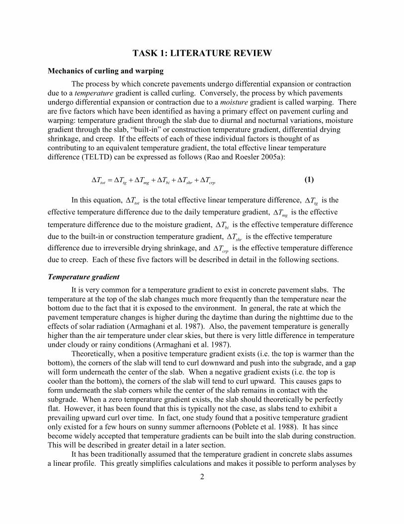
2
TASK 1: LITERATURE REVIEW
Mechanics of curling and warping The process by which concrete pavements undergo differential expansion or contraction due to a temperature gradient is called curling. Conversely, the process by which pavements undergo differential expansion or contraction due to a moisture gradient is called warping. There are five factors which have been identified as having a primary effect on pavement curling and warping: temperature gradient through the slab due to diurnal and nocturnal variations, moisture gradient through the slab, “built-in” or construction temperature gradient, differential drying shrinkage, and creep. If the effects of each of these individual factors is thought of as contributing to an equivalent temperature gradient, the total effective linear temperature difference (TELTD) can be expressed as follows (Rao and Roesler 2005a):
tot tg mg bi shr crpT T T T T T∆ = ∆ + ∆ + ∆ + ∆ + ∆ (1)
In this equation, totT∆ is the total effective linear temperature difference, tgT∆ is the effective temperature difference due to the daily temperature gradient, mgT∆ is the effective temperature difference due to the moisture gradient, biT∆ is the effective temperature difference due to the built-in or construction temperature gradient, shrT∆ is the effective temperature difference due to irreversible drying shrinkage, and crpT∆ is the effective temperature difference due to creep. Each of these five factors will be described in detail in the following sections.
Temperature gradient It is very common for a temperature gradient to exist in concrete pavement slabs. The temperature at the top of the slab changes much more frequently than the temperature near the bottom due to the fact that it is exposed to the environment. In general, the rate at which the pavement temperature changes is higher during the daytime than during the nighttime due to the effects of solar radiation (Armaghani et al. 1987). Also, the pavement temperature is generally higher than the air temperature under clear skies, but there is very little difference in temperature under cloudy or rainy conditions (Armaghani et al. 1987). Theoretically, when a positive temperature gradient exists (i.e. the top is warmer than the bottom), the corners of the slab will tend to curl downward and push into the subgrade, and a gap will form underneath the center of the slab. When a negative gradient exists (i.e. the top is cooler than the bottom), the corners of the slab will tend to curl upward. This causes gaps to form underneath the slab corners while the center of the slab remains in contact with the subgrade. When a zero temperature gradient exists, the slab should theoretically be perfectly flat. However, it has been found that this is typically not the case, as slabs tend to exhibit a prevailing upward curl over time. In fact, one study found that a positive temperature gradient only existed for a few hours on sunny summer afternoons (Poblete et al. 1988). It has since become widely accepted that temperature gradients can be built into the slab during construction. This will be described in greater detail in a later section. It has been traditionally assumed that the temperature gradient in concrete slabs assumes a linear profile. This greatly simplifies calculations and makes it possible to perform analyses by
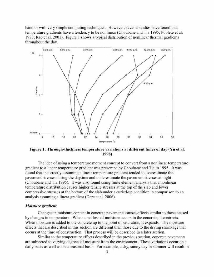
3
hand or with very simple computing techniques. However, several studies have found that temperature gradients have a tendency to be nonlinear (Choubane and Tia 1995; Poblete et al. 1988; Rao et al. 2001). Figure 1 shows a typical distribution of nonlinear thermal gradients throughout the day.
Figure 1: Through-thickness temperature variations at different times of day (Yu et al.
1998)
The idea of using a temperature moment concept to convert from a nonlinear temperature gradient to a linear temperature gradient was presented by Choubane and Tia in 1995. It was found that incorrectly assuming a linear temperature gradient tended to overestimate the pavement stresses during the daytime and underestimate the pavement stresses at night (Choubane and Tia 1995). It was also found using finite element analysis that a nonlinear temperature distribution causes higher tensile stresses at the top of the slab and lower compressive stresses at the bottom of the slab under a curled-up condition in comparison to an analysis assuming a linear gradient (Dere et al. 2006).
Moisture gradient Changes in moisture content in concrete pavements causes effects similar to those caused by changes in temperature. When a net loss of moisture occurs in the concrete, it contracts. When moisture is added to the concrete up to the point of saturation, it expands. The moisture effects that are described in this section are different than those due to the drying shrinkage that occurs at the time of construction. That process will be described in a later section. Similar to the temperature effects described in the previous section, concrete pavements are subjected to varying degrees of moisture from the environment. These variations occur on a daily basis as well as on a seasonal basis. For example, a dry, sunny day in summer will result in

4
a much different moisture gradient than a rainy, cloudy day in fall. Because the bottom of the slab is exposed to the typically moist subgrade, the moisture content in the lower section of the slab remains fairly constant and close to saturation. Most of the variations in moisture content occur in the top two inches of the slab (Yu and Khazanovich 2001). Taking all of these things into consideration, it can be concluded that the moisture gradient is generally nonlinear and that there tends to be a prevailing negative gradient (drier on top) except on wet, cloudy days when the gradient approaches zero. As noted before, the change in slab profile shape due to moisture gradient is referred to as warping and is analogous to the curling effects due to temperature gradient. Neglecting all other effects, a slab that has a lower moisture content near the top than at the bottom will warp into a shape with upward concavity. A slab that has a higher moisture content near the top than at the bottom will tend to warp into a shape with downward concavity, although the first scenario has been found to be much more common.
Built-in temperature gradient As described previously, temperature gradients in concrete pavements vary on a daily basis and cause the slab to assume a curled shape. However, it was also noted that daily fluctuations in temperature do not sufficiently describe the response that is observed in most pavement slabs. It has been known for quite some time that a zero temperature differential does not necessarily correspond to a flat slab condition. However, it was not until the late 1980s and early 1990s that the idea of a built-in or construction temperature gradient was introduced. One study performed in Munich, Germany found that constructing pavements on hot, sunny days caused the slabs to harden with a large positive temperature gradient. This resulted in a very early development of upward curling (Eisenmann and Leykauf 1990). The temperature gradient in a concrete pavement slab is always zero when it is initially placed. However, if the air temperature is warmer than the temperature of the concrete, the temperature in the top of the slab will start to increase before the concrete hardens. Because the concrete is still wet and does not have much structural integrity, it will not deform or change shape as the temperature gradient develops. Since it takes several hours for normal concrete to come to a final set, it is possible for a large temperature gradient to develop in the flat slab. If a concrete slab hardens with a positive temperature gradient, it will immediately start to curl upward as the air temperature begins to cool. As the pavement temperature near the top of the slab continues to decrease, the temperature gradient in the slab will approach zero. In other words, the slab will exhibit an upward curl at a zero temperature differential. For this reason, the slab is said to have a built-in negative temperature gradient. This makes the analysis of temperature effects in pavements simpler in that the actual temperature gradient can be added to the built-in temperature gradient to obtain the total effective gradient (Yu and Khazanovich 2001). Using this concept, the slab will only resume a flat shape when a sufficient positive temperature gradient is once again present to counteract the effective negative gradient that was built into the slab.
Differential drying shrinkage It was initially thought that the curling that was built into concrete pavement slabs was due solely to the surface shrinkage which occurred during and shortly after placement. Shrinkage can occur in two ways: through self-desiccation during the hydration process and

5
through conventional means such as evaporation (Lim et al. 2004). If it is assumed that a concrete slab hydrates uniformly throughout its thickness, then the differential drying shrinkage that occurs during construction must be due mostly to the effects of evaporation. Since the top of the slab is typically exposed to the air while the bottom of the slab rests on the subgrade, most of the moisture loss due to evaporation occurs at the top of the slab. Drying shrinkage is significantly affected by curing practices and environmental conditions, and these effects will be described in a later section. In general, the drying shrinkage that occurs during the construction process will cause the slab to assume a permanent upward curl which adds to the negative built-in temperature gradient which is typically observed. Similar to the process which occurs with temperature gradients, drying shrinkage can be partially reversed by daily and seasonal variations in moisture content at the top of the slab, but the predominant condition is that the top of the slab is drier than the bottom.
Creep Creep can be defined as time-dependent strain that occurs in a material under a constant applied stress. The strain is inelastic, so it cannot be recovered unless the direction of the applied stress is changed. A study was performed by Altoubat and Lange in 2001 which analyzed the tensile creep behavior of concrete. The specimens were restrained against movement and allowed to dry, which caused tensile stresses to develop in the concrete due to drying shrinkage. The study found that the stress relaxation which occurred due to creep effects in the samples actually doubled the shrinkage cracking strain capacity of the concrete (Altoubat and Lange 2001). Another interesting finding in this study was that sealing the samples during curing actually limited the amount of tensile creep that occurred and reduced the total shrinkage cracking strain capacity (Altoubat and Lange 2001). Finally, a test which involved periodic wetting of the samples showed that creep and shrinkage were reduced during the wetting periods and increased at a slower rate once drying resumed (Altoubat and Lange 2001). This indicates that periodically wetting concrete in its early ages can increase the shrinkage cracking strain capacity in the long term.
Creep commonly occurs in structural concrete members. For example, a non-prestressed simply-supported concrete beam loaded with gravity loads experiences a permanent downward deflection at mid-span which occurs as a result of sustained loads being applied over an extended period of time. Creep has also been found to have an effect on concrete pavements. Studies have supported the fact that creep reduces the built-in temperature gradient in concrete pavement slabs. Because a majority of pavement slabs are constructed with an effective built-in negative gradient, the corners of the slab tend to curl upward more than downward. The self-weight of the slab causes the upward deflection of the slab corners to decrease over time due to the viscous effects of creep. Also, the tensile stresses in the top of the slab due to drying shrinkage are relaxed over time. All of these effects lead to reduced curling and a more stable slab condition. One study tested a concrete highway pavement slab in Mankato, MN over a period of two years. It was found that creep effects caused the effective built-in upward curl in the slab to be reduced substantially over the two-year period (Rao et al. 2001). Another study involved the construction of a test slab in a controlled environment. Half of the slab was cured with a common curing compound while the other half was mat-cured. It was found that a significant amount of drying shrinkage occurred in the slab that was cured with curing compound. At the same time, it was found that creep strain was able to diminish some of the stresses due to drying shrinkage during the first 4 to 5 days after construction (Jeong and Zollinger 2004). These two

6
tests indicate that creep can have a significant impact on the stresses and strains in concrete pavement slabs due to curling and warping in both the early ages of the slab as well as the long-term life of the slab.
Geometric and material properties The factors introduced in the previous section describe the mechanics of slab curling and warping behavior. In this section, some of the geometric and material properties which affect curling and warping will be examined.
Concrete material properties There are a couple of concrete material properties which have a large effect on the amount of curling that occurs in pavements. The first is the coefficient of thermal expansion (CTE). As described previously, concrete expands or contracts as it undergoes changes in temperature. The amount of expansion or contraction that occurs is directly related to the coefficient of thermal expansion. The English units for CTE are strain divided by degrees Fahrenheit. The typical range for CTE in concrete is 5 x 10⁻⁶ to 7 x 10⁻⁶ in./in./°F with a mean value of 5.7 x 10⁻⁶ in./in./°F (Mallela et al. 2005). Strain due to temperature change is calculated in the following way:
* Tε α= ∆ (2)
where α is the coefficient of thermal expansion and ΔT is the change in temperature. It can be seen that a higher CTE and a greater temperature change will cause a larger amount of strain to occur. Consequently, rigid pavements constructed with concrete that has a high CTE will experience a larger amount of curling due to temperature effects. The modulus of elasticity of concrete also has an effect on the amount of curling that occurs in concrete pavements. The modulus of elasticity increases as concrete strength increases. It has been found that higher concrete strengths lead to an increased amount of curling (Bissonnette et al. 2007; Rao 2005). This could be due to the fact that higher strength concrete typically undergoes less creep and more self-desiccation.
Slab geometry The geometric characteristics of concrete pavement slabs such as length and width have a large effect on curling and warping behavior. Several studies have found that curling increases with increasing slab length (Beckemeyer et al. 2002; Heath et al. 2001; Rao et al. 2001). One study found that the amount of curling is proportional to the slab length squared (Eisenmann and Leykauf 1990). There is a point, however, when the slab becomes long enough that the self weight begins to reduce the amount of curling that can occur. This also increases the tensile stresses in the top of the slab and tends to lead to more cracking. Changes in slab width have similar effects to those due to changes in slab length. However, because of the fact that most lane widths are relatively uniform whereas joint spacing can vary substantially, most studies have focused only on the effects of slab length.

7
Slab thickness In general, curling increases as slab thickness decreases (Eisenmann and Leykauf 1990). Similar to the effect of a longer slab, a thicker slab has a larger self weight and tends to restrain the amount of upward curling that can occur. The slab thickness in relation to the base type can also have an effect on the curling stresses that occur. One study found that a thick slab on a weak subgrade developed lower curling stresses than a thin slab on a weak or strong subgrade (Reddy et al. 1963). The effects of subgrade type on curling stresses will be described in greater detail in a subsequent section.
Joint restraint mechanisms It is generally desirable to provide some sort of restraint at the joints in jointed plain concrete pavement through the use of dowel bars or simply through aggregate interlock. Dowel bars are more expensive but are also much more effective than relying on aggregate interlock. Joint restraint mechanisms cause stresses to be transferred from one slab to adjacent slabs when a load is applied near the edge of the slab. This effectively decreases the maximum magnitude of stress that must be carried by any one slab. When considering a weightless slab that curls in the absence of any external load and without any sort of joint restraint mechanism, no internal stresses develop because the edges of the slab are free to deflect as much as necessary to counteract the internal thermal gradient. However, when joint restraint mechanisms such as dowel bars or aggregate interlock are applied, the edges of the slab become restrained against vertical movement and internal stresses develop as a result. Studies have found that restrained slabs experience less vertical deflection due to curling than unrestrained slabs (Sondag and Snyder 2003; Wells et al. 2006b). The results of one of the studies can be seen in Figure 2 and Figure 3. Though these studies did not directly measure stresses in the slabs, it can be concluded that internal stresses would be higher in the slabs that were restrained due to the fact that free displacement was prevented.
Figure 2: Surface profile measurements along the transverse joint of an unrestrained slab
(Wells et al. 2006b)

8
Figure 3: Surface profile measurements along the transverse joint of a restrained slab
(Wells et al. 2006b)
The problem becomes very complex when an attempt is made to analyze the effects of traffic loads or falling-weight deflectometer (FWD) loads in addition to curling effects and load transfer devices. While the total vertical deflection of the slab edges will generally be lower in the restrained case as shown above, the internal stresses due to curling alone will be higher. Conversely, stresses due to traffic or FWD loads will be lower due to the fact that they are partially transferred to adjacent slabs. Strains measured on the bottom of the slab have been found to be reduced near restrained joints and increased near the center of the slab (Wells et al. 2006a). It has also been found that temperature gradients can have an effect on the amount of load transfer efficiency (LTE) that is present in undoweled slabs. Specifically, the LTE increases when a positive temperature gradient (downward curl) is present and decreases when a negative temperature gradient (upward curl) is present (Vandenbossche 2007).
Subgrade characteristics The type of subgrade upon which a concrete pavement slab is constructed has been found to have a significant effect on the magnitude of curling stresses that develop. It has long been understood that stronger subgrades do not necessarily result in a stronger pavement structure or allow for the use of thinner slabs (Reddy et al. 1963). Studies have shown that concrete slabs constructed on rigid subgrades such as concrete, asphalt, or other stabilized base will develop significant curling stresses and a large amount of cracking (Eisenmann and Leykauf 1990; Guo 2001). On the other hand, slabs constructed on weaker, more plastic subgrades experience lower curling stresses due to the “bedding” effect that occurs as the slab pushes into the subgrade (Dere et al. 2006; Eisenmann and Leykauf 1990). When stresses due to traffic loads are considered in addition to curling stresses, a weaker subgrade is not always the best option. One study found that a softer subgrade resulted in higher tensile stresses under combined thermal and traffic loading (Dere et al. 2006). Though the softer subgrade provides a bedding effect for slab curling, traffic loads will still cause large deflections

9
because of the minimal resistance from the subgrade. It can be concluded that an optimal subgrade stiffness exists that minimizes the stresses due to thermal and traffic loading. Curling stresses can be greatly affected by the bonding characteristics that are present between the concrete slab and the base layer. If the slab is bonded to a stabilized base, curling stresses and strains will actually be lower because both layers act as a thick composite slab (Wells et al. 2006a; Yu et al. 1998). This is not necessarily the best construction practice, however, because if the bond between the two layers is broken, the most severe case of a slab on a rigid subgrade will occur.
Effect of curling on fatigue cracking type Flat slabs with no upward or downward curl which are resting on a uniform subgrade will experience the highest internal stresses when a point load is applied at the unrestrained edge at midslab. A bending moment will form, with compressive stresses located at the top of the slab and tensile stresses located at the bottom. If the tensile stress exceeds the modulus of rupture of the concrete, a crack will form at the bottom of the slab and propagate upward to the slab surface.
Similar results occur when a slab has undergone downward curling due to a positive temperature gradient. The highest tensile stress will occur at the bottom of the slab at the location of the load. If a void is present beneath the slab at the load location, the tensile stresses will be higher than the flat slab case and the damage will be more severe (Ioannides and Salsilli-Murua 1989). Since positive temperature gradients and downward curling typically occur during the daytime when traffic loads are highest, this is usually the critical scenario.
When a sufficiently high negative temperature gradient is present in the slab and traffic loads are present, the failure mode can switch from bottom-up cracking to top-down cracking (Yu and Khazanovich 2001). Because the corners of the slab may become unsupported with a negative temperature gradient, a load placed on the corner of the slab will cause a tensile stress to form in the top fiber of the slab between the load and the middle of the slab (Ioannides and Salsilli-Murua 1989). The principle is similar to a cantilevered concrete beam with a gravity load placed on the free end. Since it is very common to have a negative built-in temperature gradient, many slabs assume a curled-up shape a majority of the time and thus experience top-down cracking as the critical failure mode. Studies have shown that top-down cracking can be limited by reducing the transverse joint spacing (Beckemeyer et al. 2002).
The figures included below show stress contours for a slab with a negative temperature gradient (curled-up condition). Figure 4 shows stresses due to thermal gradient alone (plus self weight) and Figure 5 shows stresses due to differential shrinkage and a 70 kN heavy vehicle simulator (HVS) load (represented by the two boxes). The effects due to differential shrinkage are similar to a negative temperature gradient and result in a curled-up slab.

10
Figure 4: Stress distribution for transverse cracking of a 5.3 m slab under negative
temperature gradient only (Heath et al. 2001)
Anticipated crack position

11
Figure 5: Stress distribution for corner cracking of a 3.8 m slab under 70 kN HVS loading
and differential shrinkage (Heath et al. 2001)
It can be seen that a temperature gradient acting by itself will cause the maximum tensile stress to occur at the top fiber in the center of the slab. The result is a transverse crack, provided the slab width is less than the slab length. When the slab is loaded at the corner, the maximum tensile stress develops at the top of the slab between the load and the center of the slab. A corner crack is likely to form in this situation. (Heath et al. 2001)
Factors that affect built-in curling The main focus of this research was to find a way to determine the magnitude of built-in curl from FWD deflections. Several factors have been found to affect the amount of built-in curling that occurs during construction. The effects of material properties and geometric properties have been discussed in previous sections. This section focuses on some of the construction practices that are known to directly affect the magnitude of built-in temperature gradient, including paving season, time of day, curing techniques, and mix design.
Paving season The time of year that a pavement is constructed has a significant impact on the amount of built-in curl that will occur. The type of weather that is experienced during a given season is ultimately dependent on the location. For example, the climate in the southwestern United States is primarily warm and dry with a brief rainy season while the northern United States experiences all four seasons – spring, summer, fall, and winter. In general, constructing concrete pavements in a hot, dry climate or during the summer season will result in high negative built-in
Anticipated crack positions

12
temperature gradients. Conversely, constructing pavements in a cool, wet climate or during the spring and fall will result in little or no built-in curl. Cool, moist air at the time of construction will prevent a large positive temperature gradient from forming and will also prevent drying shrinkage from occurring. One study in particular found that pavements constructed during the late fall in Michigan are less likely to develop a large amount of built-in curl and are more likely to maintain slab-base contact throughout the life of the pavement (Hansen et al. 2006).
Paving time Similar to the season during which a pavement is constructed, the time of day has a large impact on the amount of built-in curling that develops. Paving in the morning on a hot, sunny day will result in the maximum built-in temperature gradient because the slab will harden in the afternoon during the time of maximum heat and solar radiation (Hansen et al. 2006). While the temperature and moisture content at the bottom of the slab remain relatively constant, the temperature at the top of the slab increases significantly while moisture evaporates from the surface. The combined effects of temperature and drying shrinkage thus result in a large effective built-in negative temperature difference. One study looked at the effects of constructing a concrete pavement during the night and found that a significantly lower built-in curl developed compared to slabs constructed during the day (Rao et al. 2001). It can be concluded that constructing pavements late in the day or during the night in cloudy conditions will prevent significant built-in curling from occurring.
Curing techniques When a concrete pavement is constructed, various curing methods are typically employed in an attempt to prevent moisture loss and control temperature in the concrete. The effective temperature difference that is built into the slab is highly dependent on the types of curing techniques that are used. One study found that wet curing was able to reduce the amount of permanent shrinkage deformation as well as lower the temperature at the surface (Eisenmann and Leykauf 1990).
The use of a curing compound is another common way to attempt to seal the moisture inside the concrete. However, one study found that sealing concrete can actually lead to earlier cracking as a result of drying shrinkage (Altoubat and Lange 2001). Two reasons were presented for this. First of all, internal drying shrinkage due to the hydration process occurs regardless of whether or not a curing compound is applied. More importantly, when the sealant was removed, the rate of drying shrinkage increased substantially and resulted in early cracking of the samples (Altoubat and Lange 2001). Since it is possible for curing compounds to wear off in the field due to environmental effects, it can be concluded that sealing concrete is not necessarily the best way to prevent drying shrinkage and early cracking in pavements. The same study found that shrinkage stresses can be alleviated by wetting the concrete during the curing process, as shown in Figure 6 (Altoubat and Lange 2001).

13
Figure 6: Shrinkage stress under drying/wetting conditions (Altoubat and Lange 2001)
Research by Jeong and Zollinger in 2004 showed that a slab cured with an insulation mat developed less shrinkage stresses before removal of the mat than a slab cured with a typical curing compound. However, once the insulation mat was removed, shrinkage stresses developed at a rapid rate and the total upward deflection soon matched that of the membrane-cured slab (Jeong and Zollinger 2004).
Mix design The effects of concrete mix properties on built-in curling are not as prevalent as the factors that have already been discussed, but it is still a topic that is worth mentioning. Mix properties are more likely to affect the irreversible shrinkage behavior of concrete as opposed to the built-in thermal gradient. The shrinkage capacity of concrete increases as the amount of cement paste increases (Eisenmann and Leykauf 1990). This is because a higher amount of cement is available to absorb the free water in the mix. What results is a larger effective built-in negative gradient because of the irreversible drying shrinkage that occurs. A difference in shrinkage behavior is evident when comparing normal strength mixes to high strength mixes. The shrinkage gradient is dependent on many different parameters, including porosity, uneven self-desiccation, stiffness, and creep (Bissonnette et al. 2007). Though the shrinkage which occurred in the high strength mixes was lower than the normal strength mixes, the amount of curling observed in the high strength concrete was actually larger (Bissonnette et al. 2007). This discrepancy is likely due to the fact that only the ASTM C 157 length change test was used to determine the amount of shrinkage that occurred and therefore did not take into account the additional parameters that have an effect on slab curling.
Analysis and modeling of curling and warping Some understanding of the phenomenon of curling and warping in concrete pavements has been prevalent since the pioneering research performed by H. M. Westergaard in the 1920s. Since then, the advent of computing technology has allowed for significant advancements in data collection and analysis capabilities. The past 90 years have seen the refinement of empirical equations and the emergence of more accurate mechanistic procedures. The following sections

14
give a summary of the progress of curling and warping analysis throughout history and introduce several methods for back-calculating the built-in curl that is present in a slab during construction.
Historical approaches Westergaard was the first to develop a closed-form solution for calculating stresses in a concrete pavement slab that had undergone curling. However, he was forced to make several limiting assumptions in order to obtain a solution using the methods available at the time. These assumptions included a linear temperature gradient, full slab-subgrade contact (no voids), and a Winkler foundation (Reddy et al. 1963). It has already been stated that temperature gradients have been commonly found to be nonlinear and that an assumed linear temperature gradient is un-conservative when calculating slab stresses. It has also been found that the corners of a severely curled-up slab will lift off the base, creating a void underneath and causing significant tensile stresses to form in the top of the slab. While Westergaard’s solution is now considered inadequate in many respects, it served as an essential first step in the theoretical understanding of curling in concrete pavements. Many researchers over the decades have attempted to improve on Westergaard’s theory. Reddy et al. presented a theory which implemented nonlinear temperature and moisture gradients and found that this was more critical than the linear case (Reddy et al. 1963). Tang et al. developed a solution which accounted for the possibility of portions of the slab lifting off the base layer, thereby establishing a method of calculating slab stresses with a zero-support condition (Tang et al. 1993). Ioannides et al. used advanced statistical regression techniques in conjunction with artificial neural networks to evaluate the adequacy of Westergaard’s curling solution. They found that his solution was conservative in the load-only case and grossly inadequate in the scenario where only slab curling occurs (no external loads). However, they found that Westergaard’s solution compared very well with modern solution techniques when the load plus curling case was considered (Ioannides et al. 1999). This indicates that Westergaard’s solutions, while limited in scope, could still be acceptable in certain situations. The following sections focus on the ways in which modern solution techniques can be used to calculate the temperature gradient that is present in a slab and ultimately determine the amount of built-in curl that was set into the slab during construction.
Back-calculation methods It has been the focus of much research of late to find a way to back-calculate the amount of built-in curl that will occur when material, climate, geometric, and other parameters are known. The effective built-in temperature gradient is a required input for the M-E PDG (2007), but currently no method exists for determining an accurate value to use. Several back-calculation methods have been proposed by various researchers, including some combination of finite element analysis, regression analysis, and artificial neural networks, in conjunction with field tests such as surface profiling or falling weight deflectometer tests. These methods will be discussed in detail in the following sections.
Finite element method The finite element method (FEM) has become an invaluable tool in the field of pavement analysis and design. It has allowed researchers to solve many complex problems and to reevaluate some of the limiting assumptions that were imposed by the early research of

15
Westergaard and others. FEM can be used in conjunction with a computer program to develop an approximate theoretical solution to a nonlinear problem. For example, in a pavement analysis application, a pavement slab is broken up into a large number of small, discrete elements called a mesh. The corners of each element are connected to the corners of the adjacent elements at a single point called a node. Each node contains all of the defined properties of the material (in this case, concrete), which might include stiffness, Poisson’s ratio, coefficient of thermal expansion, etc. Loads and boundary conditions are applied to the mesh, and the program then conducts an iterative analysis which generally continues until it converges upon a solution. At this point, stresses, strains, and deflections can be determined at each node location. FEM has been used successfully by many researchers to develop a theoretical data set that could then be compared to field data. Heath et al. used the finite element program ISLAB2000 to predict the type of fatigue cracking that would occur in pavements with nonlinear temperature gradients (Heath et al. 2001). Guo used the program JSLAB-92 to back-calculate temperature curling in slabs (Guo 2001).
Regression analysis Regression analysis has been used extensively in the concrete pavement industry to develop empirical relationships to be used in design. It is important that when regression analysis is performed, engineering knowledge and judgment be employed throughout the process so that meaningful results can be obtained. If this is not the case, the analysis becomes simply a statistical regression which lacks the framework that is engineering mechanics (Ioannides and Salsilli-Murua 1989). Understanding the way that the independent and dependent variables interact is important if a meaningful relationship is to be obtained. Dimensional analysis, or the use of non-dimensional parameters, has emerged as a tool for developing sophisticated statistical models. This concept will be described in more detail in a later section. Though regression is not an exact science, traditional as well as advanced statistical regression techniques have been validated by extensive research. Lee and Darter (1994) developed several expressions for calculating edge bending stresses in slabs under curling-only and load-plus-curling conditions which also included the development of two new non-dimensional parameters (Lee and Darter 1994). This research was later verified by Ioannides et al. in 1994 with the use of artificial neural networks. This technique is described in the next section.
Artificial neural networks An artificial neural network (ANN) is a sophisticated computer program which uses a learning algorithm to observe patterns in a dataset to develop a solution network that is capable of giving accurate outputs based on a set of defined inputs. ANNs have been used successfully in the field of pavement design and research. One advantage of ANNs is that they are capable of handling several independent variables as inputs, which is one area where regression analysis can become tedious and unreliable. ANNs have been found to be more efficient at predicting pavement response than statistical regression equations (Ioannides et al. 1999). Overall, they are an easy-to-use tool that has been proven to be reliable and robust and will likely be implemented more and more frequently in the field of pavement design.

16
Methods of collecting field data Part of the analysis portion of this project involved using the back-calculation methods previously described to evaluate curling levels in pavements at the Minnesota Road Research Project (Mn/ROAD). The objective was to determine a way to calculate the amount of built-in curl using Falling Weight Deflectometer data in conjunction with temperature profiles. A separate task was to compare the results of the research with the results of studies where various surface profiling techniques were used. Field data collection is an important part to many research projects. It is imperative that an accurate, systematic method be used in order to obtain valid data. The quality of the research depends on the quality of the raw data that is used. Therefore, it is appropriate to spend some time discussing the various techniques that are used for the collection of pavement data. This section will focus on those techniques that are related specifically to this project.
Dipstick Auto-Read Profiler The Dipstick Auto-Read Profiler is a surface profile measurement tool that has been used extensively in determining the amount of curl that is present in concrete pavement slabs. It consists of two circular feet 12 inches apart that are connected by a device which is capable of measuring the difference in elevation between the two feet. Projecting upward from the middle of the measuring device is a vertical rod which is used to pivot the instrument 180 degrees on one of the feet, thereby allowing successive elevation measurements to be taken in a straight line across the surface of the slab. When the difference in elevation is known at several points along the straight line, a surface profile can be generated which consists of a plot of the relative slab surface elevation over the slab length. The dipstick method has been used successfully by many different researchers in developing slab surface profiles. Yu and Khazanovich showed that the Dipstick is very sensitive and significant jumps can appear in a graph of the surface profile due to very small surface irregularities. However, drawing a quadratic best-fit line through the points provided a good depiction of the overall surface profile (Yu and Khazanovich 2001). Another project used a technique of “zeroing” the Dipstick measurements in order to eliminate the noise created by surface irregularities. The method used was superior to previous methods in that it took into account the curl that was present at the time of final set (Sondag and Snyder 2003).
Falling weight deflectometer The falling weight deflectometer (FWD) is a device which consists of a circular load plate and several deflection sensors extending radially from the load plate. The dropping of the load plate onto the pavement surface is meant to simulate the weight of a vehicle wheel load as it travels over the pavement. As the plate is dropped, the load that is imparted to the pavement is measured and the deflection is measured at each of the sensor locations. FWDs are often used to measure load transfer efficiency across pavement joints. The use of FWDs has much precedent in the study of pavement curling and warping. In several studies, measured strains and deflections from FWD tests were used to verify analytical calculations performed by a computer modeling program. Also, FWD data has been used to test for voids beneath the corners of the slab. One study found that corner deflections under FWD loads were much greater during the morning than during the afternoon. This is likely due to the fact that the typical upward curl that occurs during the morning hours causes the slab corners to

17
lift off the base, resulting in a void beneath the bottom of the slab (Hansen et al. 2002). A separate study noted that voids beneath the slab can also be caused by erosion or pumping of the base layers and that care must be taken not to confuse voids due to curling with voids due to erosion (Rao and Roesler 2005b). Further research showed that temperature gradients in slabs can have an effect on FWD results and the ability to detect voids beneath the slab (Vandenbossche 2007).
MnROAD testing facility The Minnesota Road Research Project (MnROAD) is a fully-instrumented test track located about 40 miles northwest of Minneapolis, MN. About 3 miles of the track are part of Interstate 94 and are used to record data from daily vehicle traffic. The other 2.5 miles consist of a loop that is located adjacent to the highway portion and is used to measure simulated rural traffic loads. The slab instrumentation includes thermocouples, strain gages, LVDTs, tiltmeters, psychrometers, and other devices (Schmidt 2001). There is also equipment that is used to record ambient weather conditions. The MnROAD testing facility has been used in several research studies related to pavement curling and warping. One study used FWD data collected from the site over a one-year period to analyze temperature and moisture effects (Sondag and Snyder 2003). Another study used FWD data collected from Mn/ROAD to evaluate the effects of temperature gradients on load transfer efficiency and to determine whether temperature gradients affected the ability to detect voids beneath the slab (Vandenbossche 2007).
Overview of specific site studies It was stated previously that the climate and environmental conditions of a location have a large effect on pavement curling and warping. Therefore, it is of interest to examine several studies that were performed at different locations. This will help to give an idea of how various weather conditions along with assorted geometric parameters can affect the magnitude of built-in curl.
Florida DOT test road In 1982, a concrete test road was constructed at the Bureau of Materials and Research of the Florida Department of Transportation (Armaghani et al. 1987). The test road was composed of 6 slabs that were 20 feet long, 12 feet wide, and 9 inches thick. They incorporated both doweled and undoweled joints. The slabs were instrumented with thermocouples and horizontal and vertical LVDTs. The ambient air temperature was also recorded using an external thermocouple housed near the test road and weather observations were recorded on a daily basis. It was possible to record slab temperatures at 15 or 30 minute intervals at 5 different depths, allowing temperature gradients to be observed throughout the day. The study showed that pavement temperatures were generally 15-25 degrees Fahrenheit warmer than the ambient air temperature under clear skies. Very little difference in temperature was noted in cloudy and rainy weather. Also, the maximum and minimum pavement temperature was found to lag behind the maximum and minimum ambient air temperature by 1-2 hours. The slab temperature at the surface varied much more than the temperature at the bottom of the slab, resulting in varying positive and negative temperature gradients. As described previously, this is what causes slabs to undergo curling. This study also showed that temperature

18
gradients tended to be nonlinear, especially when the slabs were exposed to sudden changes in ambient temperature or moisture. Built-in curl was not very well understood at the time of this study, but it was observed that the slabs assumed a flat surface profile at a temperature gradient of about +9 °F. This was attributed to the counterbalancing effects of moisture and shrinkage, as the concept of built-in temperature gradient had not been introduced. Finally, it was found that the edges of slabs with doweled joints underwent much less horizontal displacement due to temperature effects than the edges of slabs with undoweled joints. This restrained movement can lead to increased stresses in the slab, which can become critical if combined with other stresses induced by temperature and traffic loads (Armaghani et al. 1987).
Chilean PCC in-service test road network The Chilean test road network consists of 21 separate sections that were instrumented during the extensive pavement reconstruction program of the 1970s (Poblete et al. 1988). LVDTs and thermal sensors were installed to measure horizontal and vertical slab deflections and internal temperature gradients. It was found that the temperature range at the top of the slab was four times greater than the temperature range at the bottom of the slab and that the temperature gradient was almost always nonlinear. It was also observed that large positive temperature gradients can actually cause the transverse joints to close up due to the downward rotation of the slab edges and overall horizontal expansion of the slab. Similar to the Florida DOT study, the slabs were observed to remain curled upward when no temperature gradient was present. It should be noted that the climate in the south part of Chile is significantly wetter than the climate in the north. However, the prevailing upward-curled slabs occurred throughout both climatic regions. Again, it was speculated that this was caused by the moisture differential through the slab, with the slab surface being generally drier than the bottom. The upward curling was reversed only during the afternoon on sunny days as a result of higher solar radiation (Poblete et al. 1988).
Arizona and Minnesota field tests This study consisted of testing fully-instrumented concrete pavement slabs at two different locations. The first location was Phoenix, Arizona where the slabs were placed during the night. The second location was Mankato, Minnesota where the slabs were placed during the day. The two locations are very different climatically, and this had a large effect on the curling and warping behavior of the slabs. Thermocouples were placed at four different surface locations and throughout the depth of each slab. Instrumentation also included vibrating wire strain gages, psychrometers, and gage studs. Surface profiles were obtained with the use of a Dipstick Autoread Profiler (Rao et al. 2001). The Mankato, MN section was placed at 7:30AM and hardened 6.5 hours later, resulting in a measured built-in temperature gradient of +9.6 °C (which corresponds to -9.6 °C effective built-in temperature gradient). The Phoenix, AZ section, on the other hand, was composed of 3 test cells which were placed between the hours of 1:00AM and 5:00AM. The actual built-in temperature gradient in this case was actually negative, although the exact value could not be obtained. These results indicate that paving during the night can greatly reduce or even eliminate the formation of high positive built-in temperature gradients.

19
There were several other important conclusions that were acquired as a result of this study. The test sections consisted of slabs of different lengths and different joint restraint conditions. It was found that longer slabs had a higher built-in curl and that slabs with little or no joint restraint also had a higher built-in curl. Also, the effects of shrinkage and creep were studied and it was found that long-term creep can reduce the effective built-in curl in the slab.
Michigan freeway pavement tests A doweled JPCP was constructed on I-96 near Detroit, MI in July 1997 (Hansen et al. 2002). The roadway had 12 ft lanes with 15 ft joint spacing (doweled) and a 10 ft tied PCC shoulder. Rapid development of midslab transverse cracking three years after construction (4% of slabs cracked top-down) led to an investigation of the roadway involving distress surveys, FWD tests, and surface profiling in the east-bound lane. After 4 years, 16% of slabs were cracked transversely. West-bound lanes did not experience any cracking after this time, but were constructed under different ambient conditions. The pavement was not initially instrumented during construction, so thermistor probes were inserted into the slabs during FWD testing in order to obtain a temperature profile. Surface profiles using a dipstick revealed that the slabs assumed an upward-curled shape during the morning and evening equating to a built-in gradient of -10 to -20°F for this section. Results of the FWD testing showed that much higher deflections occurred at the edges and corners during the morning and evening hours than during the afternoon. It was concluded that this was due to the loss of subgrade support caused by the upward curling of the slab during the morning and evening. It is likely that the Michigan climate during the late spring through early fall, which is characterized by warm, sunny days and clear, cool nights, contributed to the prevailing upward curling of the slabs. Also, the fact that the pavement was constructed in July indicates that a large built-in temperature gradient may be present. It should also be noted that most of the transverse cracks occurred in the outer traffic lane which indicates that fatigue loading due to truck traffic combined with temperature curl is the likely cause of premature cracking. These results were confirmed with the use of finite element tests (Hansen et al. 2002).
Pennsylvania test section Seven instrumented JPCP slabs were constructed on US Route 22 in Murrysville, PA on August 1, 2004 at approximately 7:00 am (Wells et al. 2006b). The lanes were 12 ft wide with 15 ft joint spacing, and the slabs were 12 in. thick. Three of the slabs were left undoweled so that the effects of restraint could be observed. The slabs were instrumented with temperature and moisture sensors along with strain gages. The slabs achieved a final set about 10 hours after paving, which caused a large built-in positive temperature gradient to form. The joints cracked between 17 and 19 hours after paving while a large negative temperature gradient was present. It was concluded that the stresses caused by this negative gradient were sufficient to crack the slab at the sawed joints. Surface profiles revealed that the maximum displacement due to temperature curling for unrestrained slabs was as much as twice as high as the maximum displacement for restrained slabs (Wells et al. 2006b).

20
Summary of specific site studies The studies discussed here, as well as the vast majority of other research projects, have found that JPCP slabs that are constructed in the daytime during the spring or summer months tend to have a substantial built-in negative effective temperature gradient at the time of final set. Constructing pavements at night has been shown to reduce, eliminate, or even reverse this built-in gradient. The use of wet curing has also been shown to have many beneficial effects with regard to built-in curling. Slabs with little or no joint restraint tend to undergo a larger amount of curl but also tend to experience lower surface tensile stresses than slabs with doweled joints. This can have both good and bad results, as more upward curling leads to larger voids beneath the slab and higher fatigue stresses from traffic loading. Therefore, it appears that some joint restraint is necessary to prevent premature fatigue cracking.

21
TASK 2: DEVELOPMENT OF FWD BACKCALCULATION ALGORITHM FOR BUILT-IN CURL DETERMINATION
Selection of modeling parameters The finite element modeling program ISLAB2000 was used as an analysis tool in this research project. It provided a relatively simple method of obtaining theoretical results that could be compared with measured field data from the MnROAD testing facility. The idea at the beginning of the project was to cover a very wide range of variables so as to make the results applicable to any real situation. However, it soon became clear that the number and range of variables would need to be reduced in order to complete the modeling phase of the project in a reasonable amount of time (2-3 months of continuous running). ISLAB2000 is capable of testing a large number of variables and loading scenarios. The geometric variables to be considered in this project were as follows:
• Slab width • Slab length • Shoulder type (tied PCC or none) • Slab thickness
The concrete material properties to be tested were the following:
• Modulus of elasticity • Coefficient of thermal expansion • Poisson’s ratio • Unit weight
Other parameters to be tested included:
• Load location and magnitude • Temperature difference through the slab • Modulus of subgrade reaction • Load transfer efficiency
Dimensional analysis The possibility of using dimensional analysis as a way of reducing the total modeling
time was examined. Dimensional analysis makes it possible to strategically select variables for analysis according to known relationships between certain parameters. There are at least six well-known non-dimensional ratios that have been tested in the past and found to produce accurate results for certain situations (Ioannides et al. 1999; Ioannides and Salsilli-Murua 1989). Using these ratios strategically instead of randomly testing the raw variables offered the possibility of reducing the total modeling time.
For example, looking at the ratio of slab length (L) to the radius of relative stiffness () (which depends on modulus of elasticity, slab thickness, and modulus of subgrade reaction) as a single non-dimensional variable would theoretically reduce the amount of analysis time significantly because the number of variables is reduced from four to one. However, the non-dimensional ratios cannot be input directly into ISLAB2000; instead, the inputs must be in the form of the raw variables that were listed above. In order to obtain meaningful and accurate
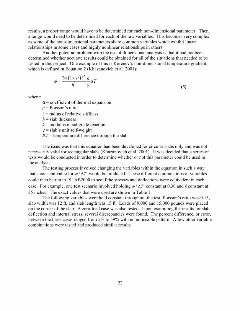
22
results, a proper range would have to be determined for each non-dimensional parameter. Then, a range would need to be determined for each of the raw variables. This becomes very complex as some of the non-dimensional parameters share common variables which exhibit linear relationships in some cases and highly nonlinear relationships in others.
Another potential problem with the use of dimensional analysis is that it had not been determined whether accurate results could be obtained for all of the situations that needed to be tested in this project. One example of this is Korenev’s non-dimensional temperature gradient, which is defined in Equation 2 (Khazanovich et al. 2001):
( ) 2
2
2 1 k Th
α µφ
γ+
= ∆
(3)
where: α = coefficient of thermal expansion μ = Poisson’s ratio = radius of relative stiffness h = slab thickness k = modulus of subgrade reaction γ = slab’s unit self-weight ΔT = temperature difference through the slab
The issue was that this equation had been developed for circular slabs only and was not necessarily valid for rectangular slabs (Khazanovich et al. 2001). It was decided that a series of tests would be conducted in order to determine whether or not this parameter could be used in the analysis.
The testing process involved changing the variables within the equation in such a way that a constant value for / Tφ ∆ would be produced. These different combinations of variables could then be run in ISLAB2000 to see if the stresses and deflections were equivalent in each case. For example, one test scenario involved holding / Tφ ∆ constant at 0.30 and constant at 35 inches. The exact values that were used are shown in Table 1.
The following variables were held constant throughout the test: Poisson’s ratio was 0.15, slab width was 12 ft, and slab length was 15 ft. Loads of 9,000 and 15,000 pounds were placed on the corner of the slab. A zero-load case was also tested. Upon examining the results for slab deflection and internal stress, several discrepancies were found. The percent difference, or error, between the three cases ranged from 5% to 59% with no noticeable pattern. A few other variable combinations were tested and produced similar results.
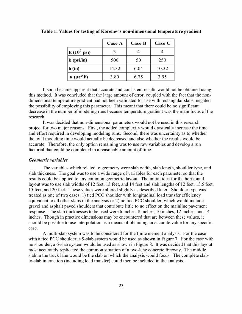
23
Table 1: Values for testing of Korenev's non-dimensional temperature gradient
Case A Case B Case C
E (106 psi) 3 4 4
k (psi/in) 500 50 250
h (in) 14.32 6.04 10.32
α (με/°F) 3.80 6.75 3.95
It soon became apparent that accurate and consistent results would not be obtained using this method. It was concluded that the large amount of error, coupled with the fact that the non-dimensional temperature gradient had not been validated for use with rectangular slabs, negated the possibility of employing this parameter. This meant that there could be no significant decrease in the number of modeling runs because temperature gradient was the main focus of the research.
It was decided that non-dimensional parameters would not be used in this research project for two major reasons. First, the added complexity would drastically increase the time and effort required in developing modeling runs. Second, there was uncertainty as to whether the total modeling time would actually be decreased and also whether the results would be accurate. Therefore, the only option remaining was to use raw variables and develop a run factorial that could be completed in a reasonable amount of time.
Geometric variables The variables which related to geometry were slab width, slab length, shoulder type, and slab thickness. The goal was to use a wide range of variables for each parameter so that the results could be applied to any common geometric layout. The initial idea for the horizontal layout was to use slab widths of 12 feet, 13 feet, and 14 feet and slab lengths of 12 feet, 13.5 feet, 15 feet, and 20 feet. These values were altered slightly as described later. Shoulder type was treated as one of two cases: 1) tied PCC shoulder with longitudinal load transfer efficiency equivalent to all other slabs in the analysis or 2) no tied PCC shoulder, which would include gravel and asphalt paved shoulders that contribute little to no effect on the mainline pavement response. The slab thicknesses to be used were 6 inches, 8 inches, 10 inches, 12 inches, and 14 inches. Though in practice dimensions may be encountered that are between these values, it should be possible to use interpolation as a means of obtaining an accurate value for any specific case. A multi-slab system was to be considered for the finite element analysis. For the case with a tied PCC shoulder, a 9-slab system would be used as shown in Figure 7. For the case with no shoulder, a 6-slab system would be used as shown in Figure 8. It was decided that this layout most accurately replicated the common situation of a two-lane concrete freeway. The middle slab in the truck lane would be the slab on which the analysis would focus. The complete slab-to-slab interaction (including load transfer) could then be included in the analysis.
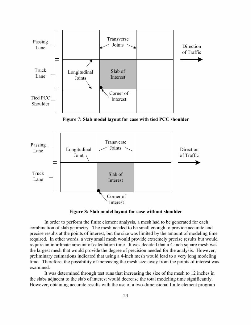
24
Figure 7: Slab model layout for case with tied PCC shoulder
Direction of Traffic
PassingLane
TruckLane
Tied PCC Shoulder
Longitudinal Joints
Transverse Joints
Slab of Interest
Corner of Interest
Direction of Traffic
Longitudinal Joint
Transverse Joints
Slab of Interest
PassingLane
TruckLane
Corner of Interest
Figure 8: Slab model layout for case without shoulder
In order to perform the finite element analysis, a mesh had to be generated for each combination of slab geometry. The mesh needed to be small enough to provide accurate and precise results at the points of interest, but the size was limited by the amount of modeling time required. In other words, a very small mesh would provide extremely precise results but would require an inordinate amount of calculation time. It was decided that a 4-inch square mesh was the largest mesh that would provide the degree of precision needed for the analysis. However, preliminary estimations indicated that using a 4-inch mesh would lead to a very long modeling time. Therefore, the possibility of increasing the mesh size away from the points of interest was examined. It was determined through test runs that increasing the size of the mesh to 12 inches in the slabs adjacent to the slab of interest would decrease the total modeling time significantly. However, obtaining accurate results with the use of a two-dimensional finite element program

25
such as ISLAB2000 requires that the aspect ratio of the mesh be square near the points of interest. It was thought that the smaller mesh spacing could be extended a certain distance beyond each edge of the middle slab to create a “buffer zone.” The spacing would then be increased to 12 inches outside of this zone. A test run was performed which involved extending the 4-inch mesh spacing 2 feet beyond each edge of the middle slab. The results of this test were then compared with the results of a test that was performed using a 4-inch mesh throughout and one that was performed without a buffer zone.
Table 2 shows a comparison of the top-of-slab stresses for the three different mesh layouts. The 4” mesh spacing can be considered the control scenario. Tensile stresses are positive whereas compressive stresses are negative. Several combinations of temperature gradient and FWD load were tested, so the magnitude and nature of the stress has a high variability. Since the purpose was simply to compare the different mesh spacings, this variability was not a concern. It can be easily seen that there was a significant improvement in results for the corner of the slab when the 2 ft buffer was added. The other slab locations showed slight improvement, but the results were not seriously inaccurate without the buffer zone. The likely reason for this is that stresses were only examined in the transverse direction. Therefore, the slab corner was the only location where the stresses were measured perpendicular to the edge of the slab.
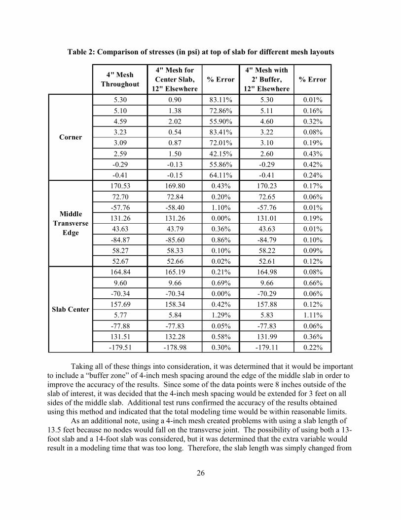
26
Table 2: Comparison of stresses (in psi) at top of slab for different mesh layouts
4" Mesh Throughout
4" Mesh for Center Slab,
12" Elsewhere% Error
4" Mesh with 2' Buffer,
12" Elsewhere% Error
Corner
5.30 0.90 83.11% 5.30 0.01%5.10 1.38 72.86% 5.11 0.16%4.59 2.02 55.90% 4.60 0.32%3.23 0.54 83.41% 3.22 0.08%3.09 0.87 72.01% 3.10 0.19%2.59 1.50 42.15% 2.60 0.43%-0.29 -0.13 55.86% -0.29 0.42%-0.41 -0.15 64.11% -0.41 0.24%
Middle Transverse
Edge
170.53 169.80 0.43% 170.23 0.17%72.70 72.84 0.20% 72.65 0.06%-57.76 -58.40 1.10% -57.76 0.01%131.26 131.26 0.00% 131.01 0.19%43.63 43.79 0.36% 43.63 0.01%-84.87 -85.60 0.86% -84.79 0.10%58.27 58.33 0.10% 58.22 0.09%52.67 52.66 0.02% 52.61 0.12%
Slab Center
164.84 165.19 0.21% 164.98 0.08%9.60 9.66 0.69% 9.66 0.66%
-70.34 -70.34 0.00% -70.29 0.06%157.69 158.34 0.42% 157.88 0.12%
5.77 5.84 1.29% 5.83 1.11%-77.88 -77.83 0.05% -77.83 0.06%131.51 132.28 0.58% 131.99 0.36%-179.51 -178.98 0.30% -179.11 0.22%
Taking all of these things into consideration, it was determined that it would be important to include a “buffer zone” of 4-inch mesh spacing around the edge of the middle slab in order to improve the accuracy of the results. Since some of the data points were 8 inches outside of the slab of interest, it was decided that the 4-inch mesh spacing would be extended for 3 feet on all sides of the middle slab. Additional test runs confirmed the accuracy of the results obtained using this method and indicated that the total modeling time would be within reasonable limits. As an additional note, using a 4-inch mesh created problems with using a slab length of 13.5 feet because no nodes would fall on the transverse joint. The possibility of using both a 13-foot slab and a 14-foot slab was considered, but it was determined that the extra variable would result in a modeling time that was too long. Therefore, the slab length was simply changed from

27
13.5 feet to 14 feet. The final slab length variables were then 12 feet, 14 feet, 15 feet, and 20 feet.
Material properties The variables that were related to concrete material properties were modulus of elasticity, coefficient of thermal expansion, Poisson’s ratio, and unit weight. It was decided initially that the Poisson’s ratio of concrete is relatively constant at 0.15, so this parameter was not varied in the analysis. The unit weight of normal-weight concrete is also fairly constant at around 150 pounds per cubic foot. It was decided early on that lightweight concrete would not be included in the analysis, so the unit weight was not included as a variable parameter.
The modulus of elasticity of concrete varies based on the compressive strength. Since this could have an effect on the calculated responses, it was decided that a range would be needed for this parameter. For normal strength concrete, the modulus of elasticity is obtained using the following relationship:
'57,000 cE f= (4)
Using this equation, a concrete strength of 3,000 psi corresponds to a modulus of elasticity of approximately 3.1 million psi. A concrete strength of 8,000 psi corresponds to a modulus of elasticity of approximately 5.1 million psi. This is at the upper end of back-calculated modulus values that are encountered in pavements today. Therefore, it was decided that the values that were to be used as inputs for modulus of elasticity were 3 million psi, 4 million psi, and 5 million psi. While it is possible that higher concrete strengths will be used in the future for certain applications, it is not expected to become widespread in the pavement industry any time soon.
The coefficient of thermal expansion of concrete was a very important parameter as the analysis focused on the response of the concrete slab to temperature gradient. As before, it was desired to use a range that would encompass all scenarios commonly found in practice. The typical range for CTE in concrete is 5 x 10⁻⁶ to 7 x 10⁻⁶ in./in./°F with a mean value of 5.7 x 10⁻⁶ in./in./°F (Mallela et al. 2005). It was assumed that the values in most cases would fall within this range. The values that were input for the modeling analysis were 4 x 10⁻⁶ in/in/°F, 5.5 x 10⁻⁶ in/in/°F, and 7 x 10⁻⁶ in/in/°F.
FWD layout Another parameter that was included in this analysis was load location and magnitude. The range of load cases used in the finite element analysis needed to encompass the load cases that were used at the MnROAD testing facility. It was hoped that in most cases a direct comparison could be made, but interpolation could be used if necessary (depending on the type of FWD used). It was decided that the most important load location to consider was the corner of the slab on the outside of the lane. This is due to the fact that upward curl tends to be the prevailing condition, so a corner load creates the highest deflection in comparison with other points on the slab. This allows for better clarity in determining the level of curling and warping present in the slab.
The load was assumed to be 8 inches square (to fit with the mesh layout) and centered at a point 4 inches vertically and horizontally from the corner of the slab. Figure 9 shows the

28
assumed FWD layout and the points at which deflections were to be measured. The deflection at Point 5 was of primary interest as it was located at the center of the load. Points 3 and 4 could be used to evaluate load transfer efficiency, and the remaining points could be used to develop deflection profiles and assess load effects. The point labeled “X” was not included in the finite element analysis because it did not fall on a node in the 4” mesh spacing, but it was shown on the diagram because it is a typical location for FWD deflection measurements. All deflection measurements and calculations in this project refer only to Point 5; although data from the other points were retained for possible use in future projects.
Figure 9: Typical FWD layout showing load location (white square) and deflection sensors
(white circles)
1
2 3 4 5 6 X 7 8 9 10 11
SlabCorner
Longitudinal Joint
Transverse Joint
12" 12" 12" 12" 12"6"6"4"8"
12"
Typical FWD loads range between 1,500 and 27,000 pounds (www.dynatest.com 2009). As before, the number of different cases that could be used in this analysis was limited by the modeling time required. The load magnitudes were set at 6,000 pounds, 9,000 pounds, and 12,000 pounds. A zero-load case was also included so that the differential displacement could be calculated.
Other parameters The other parameters that were included in the analysis were temperature difference through the slab, modulus of subgrade reaction, and load transfer efficiency. Since the study focused on the behavior of concrete pavement slabs under different temperature conditions, the temperature difference was one of the most important variables considered. Previous research has indicated that a very wide range of temperature gradients is possible in concrete pavement (Armaghani et al. 1987; Heath et al. 2001; Yu and Khazanovich 2001). It was decided that the temperature difference in this analysis would range from -80°F to +40°F in increments of 10°F. Though it would have been more desirable to use smaller temperature increments, the resulting increase in modeling time prevented this from being feasible. ISLAB2000 allows for four different subgrade foundation types: Winkler, Spring, Vlasov, or Kerr. A Winkler foundation was chosen for this study. It assumes a dense liquid foundation in which a series of linear springs supports surface loads and allows deflections only beneath the point of load application (Papagiannakis and Masad 2008). The values for the modulus of subgrade reaction (k) were chosen to be 50 psi/in, 250 psi/in, and 500 psi/in. Again, this range was assumed to adequately cover the values most commonly found in the field.

29
Load transfer efficiency (LTE), as defined in Equation 4, can vary significantly in the field both daily and seasonally and can be very difficult to control. Therefore, the entire range from zero load transfer to optimal load transfer along the transverse joints was included in the analysis with a large number of points in between.
100%U
L
LTEδδδ
= × (5)
where
δU = deflection on the unloaded side of a crack or joint and δL = deflection on the loaded side of a crack or joint
The values for transverse joint LTE that were used as inputs in ISLAB2000 were as follows (in percent): 0.1, 20, 40, 60, 80, and 99.9. ISLAB2000 was unable to run a calculation for LTE of exactly 0% or exactly 100%, so these values were approximated as shown. The longitudinal joint LTE was assumed to be 50% in all cases (including the load transfer between traffic lane and tied PCC shoulder from tie bars and aggregate interlock mechanisms).
Modeling pavement slabs with ISLAB2000 ISLAB2000 was used to calculate the slab corner deflection for every possible combination of input variables. Since there were 1,010,880 possible combinations, the modeling could not be performed in a single batch due to computing limitations. Also, different combinations of geometric properties (such as slab length and width) could not be run at the same time due to the limitations of the program. Therefore, each of the 12 combinations of slab length and width were modeled in separate batches. The total number of batches was 24, as each separate geometric layout was modeled both with and without a tied PCC shoulder. The total number of cases (or separate variable combinations) that was to be run in each batch was 42,120. However, when the first batch was started, it was discovered that the VBA code embedded in the program could only handle 32,768 rows in Microsoft Excel. To solve this problem, it was decided that the case where there was no FWD load would be run in a separate batch. This reduced the total number of cases in one batch to 31,590, which allowed the program to run without any problems. Table 3 shows how the variables slab width, slab length, and shoulder type were divided into separate batches.

30
Table 3: ISLAB2000 batch list
Batch Width (ft) Length (ft) Shoulder
1 12 12 yes2 12 14 yes3 12 15 yes4 12 20 yes5 13 12 yes6 13 14 yes7 13 15 yes8 13 20 yes9 14 12 yes
10 14 14 yes11 14 15 yes12 14 20 yes13 12 12 no14 12 14 no15 12 15 no16 12 20 no17 13 12 no18 13 14 no19 13 15 no20 13 20 no21 14 12 no22 14 14 no23 14 15 no24 14 20 no
The data that were output by ISLAB2000 were absolute deflections at the corner of the slab. In other words, the deflection was displayed in relation to a flat slab condition with negative values corresponding to upward deflections and positive values corresponding to downward deflections. It was possible to have an overall negative (upward) deflection even when a large downward load was applied if a sufficiently high negative temperature gradient was present. However, the eventual goal of the project was to compare the theoretical data calculated using ISLAB2000 with actual FWD deflection data obtained from MnROAD in order to estimate the amount of built-in curl that had occurred in the field. Because the FWD measures relative downward deflection of the slab upon application of a load, the absolute deflections obtained using ISLAB2000 had to be converted to relative downward deflections. In order to accomplish this, the modeled case with no FWD load was employed. By subtracting the unloaded absolute deflection from the absolute deflection with FWD load, it was possible to obtain the relative downward FWD deflection. The relative FWD deflection was always positive, keeping with the established sign convention of positive downward deflections.
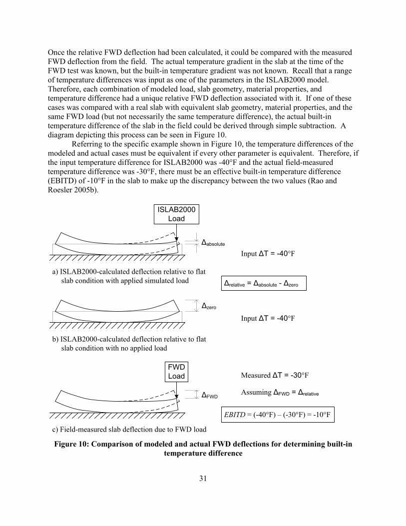
31
Once the relative FWD deflection had been calculated, it could be compared with the measured FWD deflection from the field. The actual temperature gradient in the slab at the time of the FWD test was known, but the built-in temperature gradient was not known. Recall that a range of temperature differences was input as one of the parameters in the ISLAB2000 model. Therefore, each combination of modeled load, slab geometry, material properties, and temperature difference had a unique relative FWD deflection associated with it. If one of these cases was compared with a real slab with equivalent slab geometry, material properties, and the same FWD load (but not necessarily the same temperature difference), the actual built-in temperature difference of the slab in the field could be derived through simple subtraction. A diagram depicting this process can be seen in Figure 10. Referring to the specific example shown in Figure 10, the temperature differences of the modeled and actual cases must be equivalent if every other parameter is equivalent. Therefore, if the input temperature difference for ISLAB2000 was -40°F and the actual field-measured temperature difference was -30°F, there must be an effective built-in temperature difference (EBITD) of -10°F in the slab to make up the discrepancy between the two values (Rao and Roesler 2005b).
Figure 10: Comparison of modeled and actual FWD deflections for determining built-in
temperature difference
FWD Load
ΔFWD
ISLAB2000 Load
Δabsolute
Δzero
c) Field-measured slab deflection due to FWD load
a) ISLAB2000-calculated deflection relative to flat slab condition with applied simulated load
b) ISLAB2000-calculated deflection relative to flat slab condition with no applied load
Measured ΔT = -30°F
Input ΔT = -40°F
Input ΔT = -40°F
Assuming ΔFWD = Δrelative
Δrelative = Δabsolute - Δzero
EBITD = (-40°F) – (-30°F) = -10°F

32
It soon became apparent that using the process of finding a modeled slab that was equivalent with a specific slab in the field in order to determine the built-in temperature difference would be extremely tedious, especially if a large number of trials were to be performed. Also, in the case that there was no modeled slab to match an actual slab, interpolation would prove to be very difficult because the relationships between variables were mostly nonlinear. Therefore, it was concluded that some sort of algorithm or regression equation would need to be developed in order to easily and accurately solve for temperature difference given a specific slab condition.
Data-fitting techniques In this project, two different techniques were used experimentally in order to determine the best way of fitting the data. It was important that a good fit be achieved so that accurate comparisons could be made with actual field data. The standards for a good fit could be set higher because the source of the data was a theoretical model and not a lab or field experiment. Therefore, it was desirable to obtain r2 values of at least 0.99. The proposed method for fitting the data involved using the following model parameters as independent variables: subgrade stiffness, slab length, slab thickness, modulus of elasticity, coefficient of thermal expansion, load transfer efficiency, applied FWD load, and relative FWD deflection. The top-to-bottom temperature difference was then set as the desired output variable. In this way, an equation or network could be developed which would allow the user to input actual slab parameters and FWD test data and solve for the temperature difference. This value could then be compared to the actual temperature difference measured at the time of the FWD test and the built-in temperature difference could be calculated by subtracting the two values.
The two data-fitting methods that were used were regression analysis and artificial neural networks. A trial was performed using each method, and it was observed that artificial neural networks gave superior results. A brief description of the regression analysis technique is given, but the main focus is on the artificial neural networks.
Regression analysis The first data-fitting technique that was tried was regression analysis with the use of the software program DataFit 9.0 from Oakdale Engineering (www.curvefitting.com 2009). This program employed nonlinear regression techniques to develop equations to solve for the temperature difference. First, a set of ISLAB2000 data (one batch) was imported into the DataFit program. The independent variables were defined as those listed in the previous section. It should be noted that slab length (i.e. joint spacing) was not included as an independent variable in these trial runs because data from only one batch was being tested. Temperature difference was set as the dependent variable. A generalized regression equation was then defined as shown below, with the variables X1 through X7 corresponding to the independent variables and Y being the dependent variable.
* 1 * 2 * 3 * 4 * 5 * 6 * 7Y a X b X c X d X e X f X g X h= + + + + + + + (6)
This equation was applied to the data set, and the program went through several iterations to solve for the coefficients a through h. The standard error and coefficient of multiple determination (r2) were calculated and presented with the solution. The simple relationship

33
shown above was only able to achieve an r2 value of about 0.84, which was well below the target value of 0.99. Subsequently, more complicated relationships were tested and most were found to give a better relationship than the equation with simple linear terms. For example, a better fit was achieved when the slab thickness was squared or cubed, the FWD load was squared, and the LTE and subgrade terms were raised to the one-half power. Several different combinations of exponents and various operators were tried on different variables, but the best relationship that was achieved had an r2 value of only 0.91. It was proposed that the use of non-dimensional parameters could lead to a more accurate solution due to the possible reduction of variables and the more fundamental relationships involved. Some of the non-dimensional parameters that were tried included the following:
• AGG
k
•
a
• Dγ • PD
The first two are well-known parameters, where AGG is the aggregate interlock factor, k is
the subgrade stiffness, is the radius of relative stiffness, and a is the load radius. Dγ and DP are parameters that were introduced in a report by Lee and Darter and represent effects due to slab weight and external load, respectively (Lee and Darter 1994). However, substituting these non-dimensional parameters failed to produce better results after several trials, and this idea was consequently abandoned. It soon became apparent that the regression analysis software would not be capable of producing the desired results. It was therefore decided that another method of fitting the data would need to be explored. As an emerging technology that has proven to be very reliable under several different circumstances, an artificial neural network was chosen as the next data-fitting technique for evaluation.
Artificial neural network When the regression analysis software failed to produce the desired results, it was decided that an artificial neural network (ANN) would be used to analyze the data set. ANNs were introduced in previously. The software program NeuroSolutions for Excel, Version 5 was used to create the ANN (www.nd.com 2009). The process used to develop and train the network will be described in detail in the following sections. Overall, the use of ANNs provided satisfactory results and allowed for the continuation of the research project.
Development of artificial neural network
Background on ANNs In this research, a basic Multilayer Perceptron Network (MLP) was used to analyze the
data. An MLP generally consists of three layers of nodes – an input layer, a hidden layer, and an output layer. Two or more hidden layers may be used, although using several hidden layers is

34
not recommended as this can cause the network to memorize the dataset instead of find a generalized pattern. The input layer contains as many nodes as independent variables, and the output layer contains as many nodes as dependent variables. The nodes are also referred to as processing elements (PEs). The hidden layer can contain as many PEs as the user wishes to include, although a larger number of PEs will result in a longer learning time for the network and possible memorization of the data. The network operates by feeding defined input values through the system several times until it has learned the pattern and the generated output values are very close to the desired output values. A sample generic MLP network can be seen in Figure 11. The process begins by normalizing the input values so that the range is between -1 and 1. As the input values are fed into the hidden layer, a weight (Wh) is applied and a new value is created (u). This value is then fed through a transfer function (σ) to generate the value h. Another weight (Wy) is applied to produce the value v and a final transfer function is used to generate the output. This process is then repeated hundreds or thousands of times, adjusting the weights each time based on the error of the previous run, until the network converges on a solution. The program uses mean squared error (MSE) as the parameter which determines when an adequate solution has been obtained. The user defines the minimum MSE and/or the maximum number of training runs (epochs) so that the program knows how long it should continue the solving process.
Figure 11: Example of MLP artificial neural network (http://www.dtreg.com/mlfn.htm)
Development of training set It was decided that the optimal network for this project would be experimentally
determined. The focus was first placed on developing an adequate network for the data from one batch only. It was thought that this network could then be trained on the data from the other batches to produce the desired results. In general, about 50% of the data was used for training the network, 10% was used for cross validation, and the remaining data was used to test or verify the accuracy of the network. Using cross validation during the training phase helped to ensure that the network was not simply memorizing the data. The testing phase was the most important as far as determining the accuracy of the network because it displayed a direct comparison between desired responses and actual responses and also produced a table with values for statistical evaluation. This table included an r value (not r2), mean squared error (MSE), mean absolute error (MAE), and

35
absolute maximum error. The data was always randomized before training so that the network was trained on the full range of each input variable. The variables used as inputs were subgrade stiffness, slab thickness, modulus of elasticity, coefficient of thermal expansion, load transfer efficiency, applied FWD load, and relative FWD deflection. At first, an attempt was made to develop a network that was based on the entire range of every input variable. However, the results were very poor, with r values between 0.74 and 0.78 (which translates to r2 values of 0.55 and 0.61), an MSE of 550°F, and an MAE of 18°F. It was thought that the reason for the poor fit was that the zero load case was being included as part of the dataset. When zero load is applied, the relative FWD deflection is always zero, no matter what combination of input variables is used. As it would be impossible to recognize any meaningful pattern in such a dataset, it was concluded that this is what was causing the ANN to give poor results. When all cases with zero FWD load had been removed from the dataset, the ANN produced significantly better results, with r values around 0.90, MSE of about 250°F, and MAE around 12°F. Though this was a very large improvement, the results were still not nearly as good as they needed to be. When the testing data is run through the network, a list is created which shows the actual temperature difference alongside the temperature difference predicted by the network. This allows the user to observe the error that occurs in each individual case. Utilizing this feature, it was discovered that most of the error occurred in cases where the temperature difference was between 0°F and 40°F. In other words, the ANN was having a very difficult time predicting positive temperature difference. It was hypothesized that the reason for this was that the slab was in contact with the subgrade at this range of temperatures. This would greatly reduce the relative deflection caused by the FWD load and possibly lead to irregularities in the data. To test this hypothesis, relative deflection was plotted as a function of temperature difference for a single combination of slab properties and subgrade type. This plot can be seen in Figure 12. The three separate curves represent the three FWD loads. The discrepancy between the pattern in the negative temperature range and the pattern in the positive temperature range can be clearly seen.
It was thought that breaking the dataset into two separate groups – one encompassing the range of negative temperature difference and the other incorporating the range of positive temperature difference – would help the ANN to better recognize the pattern in each set. First, a network was trained on data which only included temperature differences between -80°F and -10°F. The results showed significant improvement, with an r value of 0.991 (r2 of 0.982), MSE of 9.7°F, and MAE of 2.1°F. This was very close to the target r2 value of 0.99. However, when the network was trained on data which only included temperature differences between 0°F and 40°F, the results were much worse with the r value dropping to 0.84. Referring to Figure 12, it was concluded that the network was having difficulty predicting positive temperature difference because the curve was nearly perpendicular to the relative deflection axis in that range for FWD loads placed at the corner of the slab. This may not necessarily be the case for loaded areas at the center of the slab where unsupported portions of the slabs may occur under a positive temperature gradient.
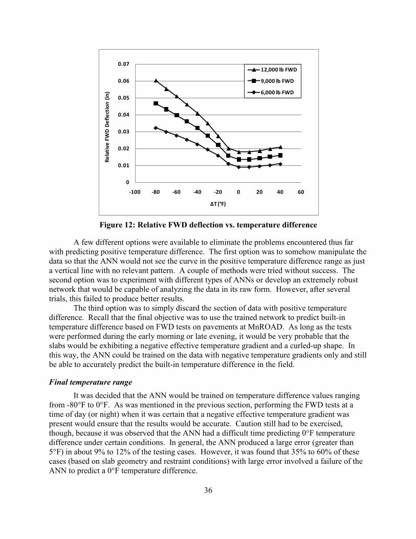
36
Figure 12: Relative FWD deflection vs. temperature difference
0
0.01
0.02
0.03
0.04
0.05
0.06
0.07
-100 -80 -60 -40 -20 0 20 40 60
Rela
tive
FW
D D
efle
ctio
n (in
)
ΔT (°F)
12,000 lb FWD
9,000 lb FWD
6,000 lb FWD
A few different options were available to eliminate the problems encountered thus far with predicting positive temperature difference. The first option was to somehow manipulate the data so that the ANN would not see the curve in the positive temperature difference range as just a vertical line with no relevant pattern. A couple of methods were tried without success. The second option was to experiment with different types of ANNs or develop an extremely robust network that would be capable of analyzing the data in its raw form. However, after several trials, this failed to produce better results. The third option was to simply discard the section of data with positive temperature difference. Recall that the final objective was to use the trained network to predict built-in temperature difference based on FWD tests on pavements at MnROAD. As long as the tests were performed during the early morning or late evening, it would be very probable that the slabs would be exhibiting a negative effective temperature gradient and a curled-up shape. In this way, the ANN could be trained on the data with negative temperature gradients only and still be able to accurately predict the built-in temperature difference in the field.
Final temperature range It was decided that the ANN would be trained on temperature difference values ranging from -80°F to 0°F. As was mentioned in the previous section, performing the FWD tests at a time of day (or night) when it was certain that a negative effective temperature gradient was present would ensure that the results would be accurate. Caution still had to be exercised, though, because it was observed that the ANN had a difficult time predicting 0°F temperature difference under certain conditions. In general, the ANN produced a large error (greater than 5°F) in about 9% to 12% of the testing cases. However, it was found that 35% to 60% of these cases (based on slab geometry and restraint conditions) with large error involved a failure of the ANN to predict a 0°F temperature difference.
37
Referring back to Figure 12 on page 36, it can be seen that the 0°F temperature difference does not fit in with the curve for negative temperature difference. It was thought that perhaps the ANN was trying to fit the 0°F temperature difference to the pattern for negative temperature difference and then labeling it as an outlier when the point did not fit on the curve. The idea was presented that including additional data points between -10°F and 0°F might help the ANN to fit the curve better. Additional finite element runs were performed with ISLAB2000, this time using temperature differences of -8°F, -6°F, -4°F, and -2°F. All other variables remained the same. As this was merely a trial, an analysis of only one geometric layout was performed (12’ x 12’ slab with tied PCC shoulder). Once the additional data points had been generated, they were input into the main dataset and the ANN was trained. Upon testing the network, no significant improvement was found. Testing results before adding the additional data points showed an r value of 0.989, MSE of 15.1°F, and MAE of 2.6°F. After adding the additional temperature difference values, the testing results showed an r value of 0.991, MSE of 13.8, and MAE of 2.6. Because the results were not significantly improved and the task of performing additional finite element analyses would take an inordinate amount of time, the idea was abandoned.
Final network architecture It was decided after several trial runs that joint spacing should be added as a training variable. In this way, any joint spacing between 12 ft and 20 ft could be input into the network and no additional interpolation would need to be performed. For example, if the ANN did not include joint spacing as a training variable and it was desired to test a slab length of 16 feet, the network would have to be run twice – once with a 15 ft joint spacing and once with a 20 ft joint spacing. Then, in order to obtain the correct temperature gradient for a 16 ft joint spacing, interpolation between the two network outputs would have to be performed. Since the relationship is nonlinear, this process would prove to be very difficult and likely inaccurate. With joint spacing included as a variable, a total of six networks needed to be trained – one each for a lane width of 12 ft, 13 ft, and 14 ft; with and without a tied PCC shoulder. It was assumed that most pavements have a slab width that is exactly one of the three mentioned (no half-foot measurements), so no interpolation is anticipated.
After a significant number of trial networks had been created, trained, and tested, a number of conclusions could be made. A larger network produced slightly better results at the expense of an increased training time. A smaller network trained more quickly but produced inferior results. It was also theorized that a using an exact multiple of the number of independent variables would create symmetry and optimize the network. Taking all of these things into consideration, it was determined that the optimal ANN architecture included two hidden layers with 64 processing elements in each layer. Using 40,000 (out of approximately 87,500) rows for training and 30,000 training epochs, the network required around 23 hours to learn the data. It performed reasonably well in testing, with an r value of approximately 0.991, MSE of 12.7°F, and MAE of 2.5°F.
Error susceptibility and statistical summary Once the final ANN architecture had been decided upon, the data was broken down into groups of four batches. Each group represented a specific lane width and shoulder type, and the four batches in each group represented the four different joint spacings. All six groups were trained separately using the format described in the previous section. Upon completion of
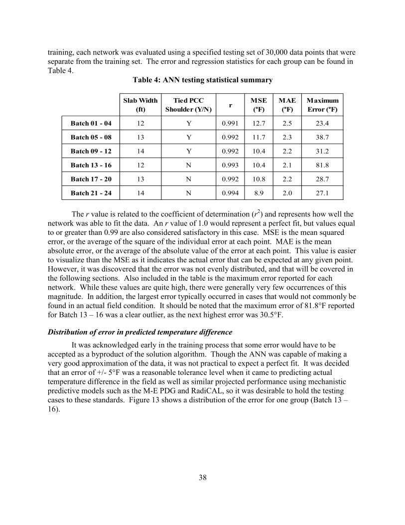
38
training, each network was evaluated using a specified testing set of 30,000 data points that were separate from the training set. The error and regression statistics for each group can be found in Table 4.
Table 4: ANN testing statistical summary
Slab Width (ft)
Tied PCC Shoulder (Y/N) r
MSE (°F)
MAE (°F)
Maximum Error (°F)
Batch 01 - 04 12 Y 0.991 12.7 2.5 23.4
Batch 05 - 08 13 Y 0.992 11.7 2.3 38.7
Batch 09 - 12 14 Y 0.992 10.4 2.2 31.2
Batch 13 - 16 12 N 0.993 10.4 2.1 81.8
Batch 17 - 20 13 N 0.992 10.8 2.2 28.7
Batch 21 - 24 14 N 0.994 8.9 2.0 27.1
The r value is related to the coefficient of determination (r2) and represents how well the network was able to fit the data. An r value of 1.0 would represent a perfect fit, but values equal to or greater than 0.99 are also considered satisfactory in this case. MSE is the mean squared error, or the average of the square of the individual error at each point. MAE is the mean absolute error, or the average of the absolute value of the error at each point. This value is easier to visualize than the MSE as it indicates the actual error that can be expected at any given point. However, it was discovered that the error was not evenly distributed, and that will be covered in the following sections. Also included in the table is the maximum error reported for each network. While these values are quite high, there were generally very few occurrences of this magnitude. In addition, the largest error typically occurred in cases that would not commonly be found in an actual field condition. It should be noted that the maximum error of 81.8°F reported for Batch 13 – 16 was a clear outlier, as the next highest error was 30.5°F.
Distribution of error in predicted temperature difference It was acknowledged early in the training process that some error would have to be accepted as a byproduct of the solution algorithm. Though the ANN was capable of making a very good approximation of the data, it was not practical to expect a perfect fit. It was decided that an error of +/- 5°F was a reasonable tolerance level when it came to predicting actual temperature difference in the field as well as similar projected performance using mechanistic predictive models such as the M-E PDG and RadiCAL, so it was desirable to hold the testing cases to these standards. Figure 13 shows a distribution of the error for one group (Batch 13 – 16).
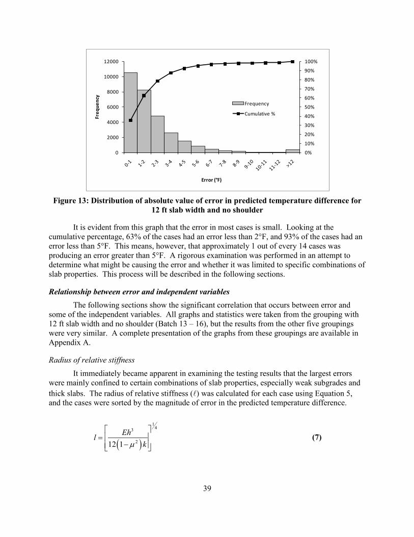
39
Figure 13: Distribution of absolute value of error in predicted temperature difference for
12 ft slab width and no shoulder
0%
10%
20%
30%
40%
50%
60%
70%
80%
90%
100%
0
2000
4000
6000
8000
10000
12000
Freq
uenc
y
Error (°F)
Frequency
Cumulative %
It is evident from this graph that the error in most cases is small. Looking at the cumulative percentage, 63% of the cases had an error less than 2°F, and 93% of the cases had an error less than 5°F. This means, however, that approximately 1 out of every 14 cases was producing an error greater than 5°F. A rigorous examination was performed in an attempt to determine what might be causing the error and whether it was limited to specific combinations of slab properties. This process will be described in the following sections.
Relationship between error and independent variables The following sections show the significant correlation that occurs between error and
some of the independent variables. All graphs and statistics were taken from the grouping with 12 ft slab width and no shoulder (Batch 13 – 16), but the results from the other five groupings were very similar. A complete presentation of the graphs from these groupings are available in Appendix A.
Radius of relative stiffness It immediately became apparent in examining the testing results that the largest errors were mainly confined to certain combinations of slab properties, especially weak subgrades and thick slabs. The radius of relative stiffness () was calculated for each case using Equation 5, and the cases were sorted by the magnitude of error in the predicted temperature difference.
( )
143
212 1Ehl
kµ
=
− (7)
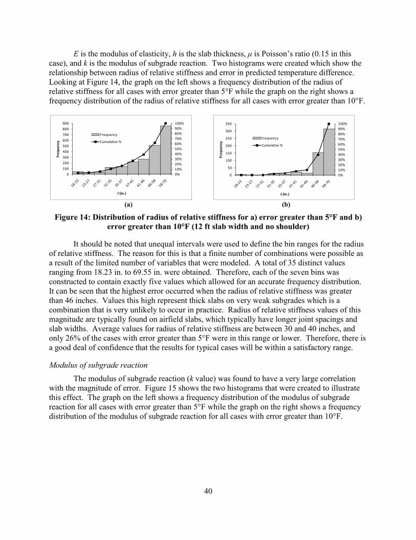
40
E is the modulus of elasticity, h is the slab thickness, μ is Poisson’s ratio (0.15 in this case), and k is the modulus of subgrade reaction. Two histograms were created which show the relationship between radius of relative stiffness and error in predicted temperature difference. Looking at Figure 14, the graph on the left shows a frequency distribution of the radius of relative stiffness for all cases with error greater than 5°F while the graph on the right shows a frequency distribution of the radius of relative stiffness for all cases with error greater than 10°F.
(a) (b)
Figure 14: Distribution of radius of relative stiffness for a) error greater than 5°F and b) error greater than 10°F (12 ft slab width and no shoulder)
0%10%20%30%40%50%60%70%80%90%100%
0
100
200
300
400
500
600
700
800
900
Freq
uenc
y
l (in.)
Frequency
Cumulative %
It should be noted that unequal intervals were used to define the bin ranges for the radius of relative stiffness. The reason for this is that a finite number of combinations were possible as a result of the limited number of variables that were modeled. A total of 35 distinct values ranging from 18.23 in. to 69.55 in. were obtained. Therefore, each of the seven bins was constructed to contain exactly five values which allowed for an accurate frequency distribution. It can be seen that the highest error occurred when the radius of relative stiffness was greater than 46 inches. Values this high represent thick slabs on very weak subgrades which is a combination that is very unlikely to occur in practice. Radius of relative stiffness values of this magnitude are typically found on airfield slabs, which typically have longer joint spacings and slab widths. Average values for radius of relative stiffness are between 30 and 40 inches, and only 26% of the cases with error greater than 5°F were in this range or lower. Therefore, there is a good deal of confidence that the results for typical cases will be within a satisfactory range.
Modulus of subgrade reaction The modulus of subgrade reaction (k value) was found to have a very large correlation with the magnitude of error. Figure 15 shows the two histograms that were created to illustrate this effect. The graph on the left shows a frequency distribution of the modulus of subgrade reaction for all cases with error greater than 5°F while the graph on the right shows a frequency distribution of the modulus of subgrade reaction for all cases with error greater than 10°F.
0%10%20%30%40%50%60%70%80%90%100%
0
50
100
150
200
250
300
350
Freq
uenc
y
l (in.)
Frequency
Cumulative %

41
(a) (b)
Figure 15: Distribution of modulus of subgrade reaction for a) error greater than 5°F and b) error greater than 10°F (12 ft slab width and no shoulder)
0%
10%
20%
30%
40%
50%
60%
70%
80%
90%
100%
0
200
400
600
800
1000
1200
1400
1600
1800
50 250 500
Freq
uenc
y
k (psi/in.)
Frequency
Cumulative %
It can be seen that the largest error occurs almost exclusively in cases where the k value is only 50 psi/in. In fact, 74% of the cases with error greater than 5°F had a k value of 50 psi/in., and only 3 cases out of 523 with error greater than 10°F had a k value of 250 psi/in. or 500 psi/in. While it is rare to have a subgrade with a k value of only 50 psi/in., there will be cases when the ANN software will have to interpolate between 50 psi/in. and 250 psi/in. Therefore, when the k value is at the lower end of this interval, the accuracy of the results may be put into question. While it may appear that any predicted results for a weak subgrade will be inaccurate and unusable, this is actually not the case. Only 16% of the cases with a k value of 50 psi/in. had an error greater than 5°F. Therefore, as it was suggested in the previous section, caution should be exercised when a weak subgrade is used in conjunction with certain ranges of other independent variables such as slab thickness.
Slab thickness The correlation between slab thickness and error was similar to the trend for radius of relative stiffness. Figure 16 shows the two histograms that were created to depict the relationship. The graph on the left shows a frequency distribution of the slab thickness for all cases with error greater than 5°F while the graph on the right shows a frequency distribution of the slab thickness for all cases with error greater than 10°F.
(a) (b)
Figure 16: Distribution of slab thickness for a) error greater than 5°F and b) error greater than 10°F (12 ft slab width and no shoulder)
0%10%20%30%40%50%60%70%80%90%100%
0
100
200
300
400
500
600
50 250 500
Freq
uenc
y
k (psi/in.)
Frequency
Cumulative %
0%
10%
20%
30%
40%
50%
60%
70%
80%
90%
100%
0
100
200
300
400
500
600
700
800
900
1000
6 8 10 12 14
Freq
uenc
y
h (in.)
Frequency
Cumulative %
0%
10%
20%
30%
40%
50%
60%
70%
80%
90%
100%
0
50
100
150
200
250
6 8 10 12 14
Freq
uenc
y
h (in.)
Frequency
Cumulative %
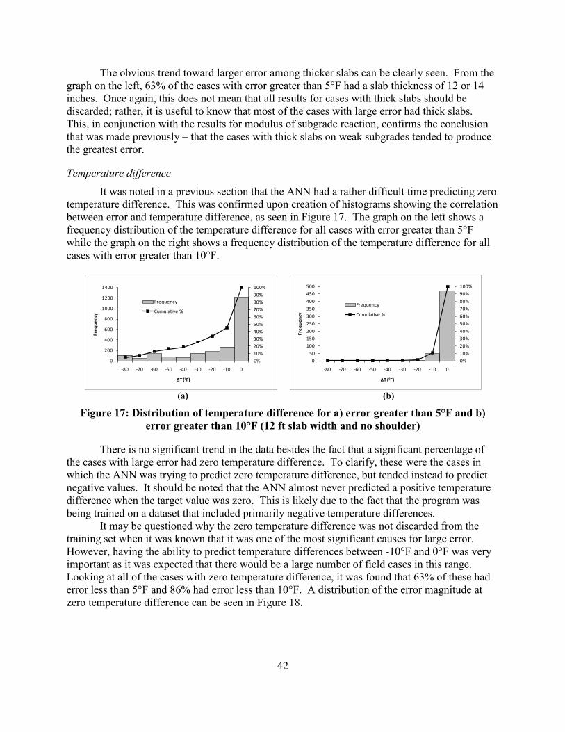
42
The obvious trend toward larger error among thicker slabs can be clearly seen. From the graph on the left, 63% of the cases with error greater than 5°F had a slab thickness of 12 or 14 inches. Once again, this does not mean that all results for cases with thick slabs should be discarded; rather, it is useful to know that most of the cases with large error had thick slabs. This, in conjunction with the results for modulus of subgrade reaction, confirms the conclusion that was made previously – that the cases with thick slabs on weak subgrades tended to produce the greatest error.
Temperature difference It was noted in a previous section that the ANN had a rather difficult time predicting zero temperature difference. This was confirmed upon creation of histograms showing the correlation between error and temperature difference, as seen in Figure 17. The graph on the left shows a frequency distribution of the temperature difference for all cases with error greater than 5°F while the graph on the right shows a frequency distribution of the temperature difference for all cases with error greater than 10°F.
(a) (b)
Figure 17: Distribution of temperature difference for a) error greater than 5°F and b) error greater than 10°F (12 ft slab width and no shoulder)
0%10%20%30%40%50%60%70%80%90%100%
0
200
400
600
800
1000
1200
1400
-80 -70 -60 -50 -40 -30 -20 -10 0
Freq
uenc
y
ΔT (°F)
Frequency
Cumulative %
There is no significant trend in the data besides the fact that a significant percentage of the cases with large error had zero temperature difference. To clarify, these were the cases in which the ANN was trying to predict zero temperature difference, but tended instead to predict negative values. It should be noted that the ANN almost never predicted a positive temperature difference when the target value was zero. This is likely due to the fact that the program was being trained on a dataset that included primarily negative temperature differences. It may be questioned why the zero temperature difference was not discarded from the training set when it was known that it was one of the most significant causes for large error. However, having the ability to predict temperature differences between -10°F and 0°F was very important as it was expected that there would be a large number of field cases in this range. Looking at all of the cases with zero temperature difference, it was found that 63% of these had error less than 5°F and 86% had error less than 10°F. A distribution of the error magnitude at zero temperature difference can be seen in Figure 18.
0%
10%
20%
30%
40%
50%
60%
70%
80%
90%
100%
0
50
100
150
200
250
300
350
400
450
500
-80 -70 -60 -50 -40 -30 -20 -10 0
Freq
uenc
y
ΔT (°F)
Frequency
Cumulative %
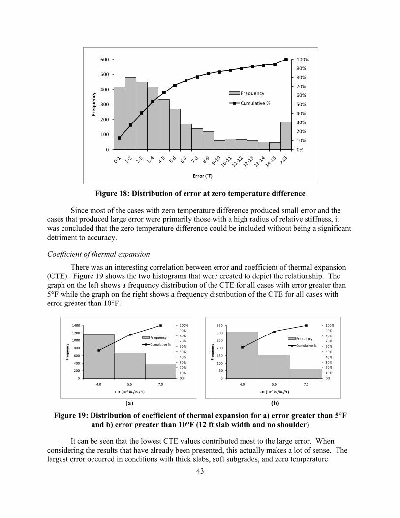
43
Figure 18: Distribution of error at zero temperature difference
0%
10%
20%
30%
40%
50%
60%
70%
80%
90%
100%
0
100
200
300
400
500
600
Freq
uenc
y
Error (°F)
Frequency
Cumulative %
Since most of the cases with zero temperature difference produced small error and the cases that produced large error were primarily those with a high radius of relative stiffness, it was concluded that the zero temperature difference could be included without being a significant detriment to accuracy.
Coefficient of thermal expansion There was an interesting correlation between error and coefficient of thermal expansion (CTE). Figure 19 shows the two histograms that were created to depict the relationship. The graph on the left shows a frequency distribution of the CTE for all cases with error greater than 5°F while the graph on the right shows a frequency distribution of the CTE for all cases with error greater than 10°F.
(a) (b)
Figure 19: Distribution of coefficient of thermal expansion for a) error greater than 5°F and b) error greater than 10°F (12 ft slab width and no shoulder)
0%
10%
20%
30%
40%
50%
60%
70%
80%
90%
100%
0
200
400
600
800
1000
1200
1400
4.0 5.5 7.0
Freq
uenc
y
CTE (10-6 in./in./°F)
Frequency
Cumulative %
It can be seen that the lowest CTE values contributed most to the large error. When considering the results that have already been presented, this actually makes a lot of sense. The largest error occurred in conditions with thick slabs, soft subgrades, and zero temperature
0%
10%
20%
30%
40%
50%
60%
70%
80%
90%
100%
0
50
100
150
200
250
300
350
4.0 5.5 7.0
Freq
uenc
y
CTE (10-6 in./in./°F)
Frequency
Cumulative %
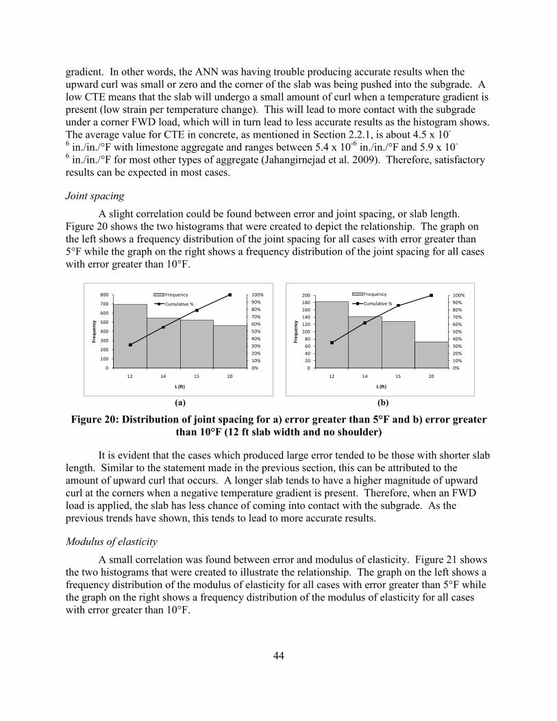
44
gradient. In other words, the ANN was having trouble producing accurate results when the upward curl was small or zero and the corner of the slab was being pushed into the subgrade. A low CTE means that the slab will undergo a small amount of curl when a temperature gradient is present (low strain per temperature change). This will lead to more contact with the subgrade under a corner FWD load, which will in turn lead to less accurate results as the histogram shows. The average value for CTE in concrete, as mentioned in Section 2.2.1, is about 4.5 x 10-
6 in./in./°F with limestone aggregate and ranges between 5.4 x 10⁻⁶ in./in./°F and 5.9 x 10-
6 in./in./°F for most other types of aggregate (Jahangirnejad et al. 2009). Therefore, satisfactory results can be expected in most cases.
Joint spacing A slight correlation could be found between error and joint spacing, or slab length. Figure 20 shows the two histograms that were created to depict the relationship. The graph on the left shows a frequency distribution of the joint spacing for all cases with error greater than 5°F while the graph on the right shows a frequency distribution of the joint spacing for all cases with error greater than 10°F.
(a) (b)
Figure 20: Distribution of joint spacing for a) error greater than 5°F and b) error greater than 10°F (12 ft slab width and no shoulder)
0%
10%
20%
30%
40%
50%
60%
70%
80%
90%
100%
0
100
200
300
400
500
600
700
800
12 14 15 20
Freq
uenc
y
L (ft)
Frequency
Cumulative %
It is evident that the cases which produced large error tended to be those with shorter slab length. Similar to the statement made in the previous section, this can be attributed to the amount of upward curl that occurs. A longer slab tends to have a higher magnitude of upward curl at the corners when a negative temperature gradient is present. Therefore, when an FWD load is applied, the slab has less chance of coming into contact with the subgrade. As the previous trends have shown, this tends to lead to more accurate results.
Modulus of elasticity A small correlation was found between error and modulus of elasticity. Figure 21 shows the two histograms that were created to illustrate the relationship. The graph on the left shows a frequency distribution of the modulus of elasticity for all cases with error greater than 5°F while the graph on the right shows a frequency distribution of the modulus of elasticity for all cases with error greater than 10°F.
0%10%20%30%40%50%60%70%80%90%100%
020406080
100120140160180200
12 14 15 20
Freq
uenc
y
L (ft)
Frequency
Cumulative %
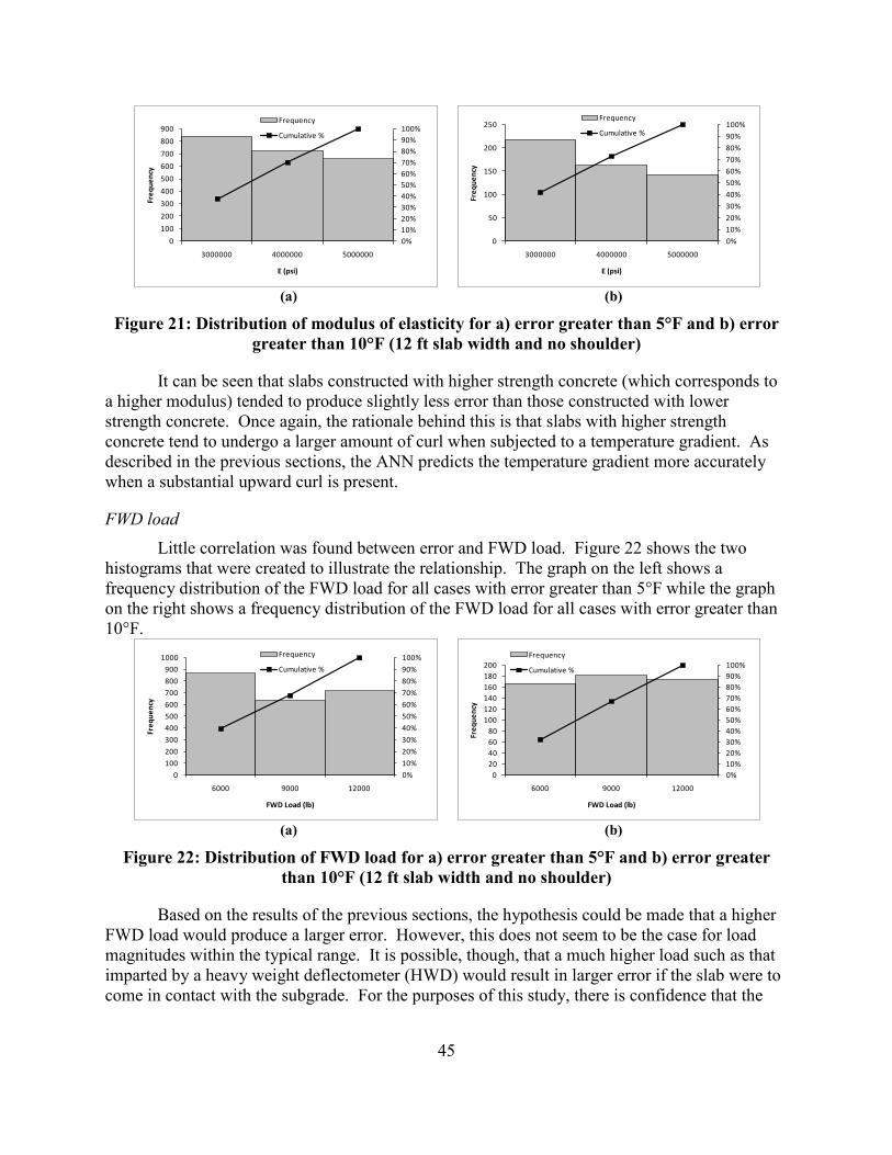
45
(a) (b)
Figure 21: Distribution of modulus of elasticity for a) error greater than 5°F and b) error greater than 10°F (12 ft slab width and no shoulder)
0%10%20%30%40%50%60%70%80%90%100%
0
100
200
300
400
500
600
700
800
900
3000000 4000000 5000000
Freq
uenc
y
E (psi)
Frequency
Cumulative %
It can be seen that slabs constructed with higher strength concrete (which corresponds to a higher modulus) tended to produce slightly less error than those constructed with lower strength concrete. Once again, the rationale behind this is that slabs with higher strength concrete tend to undergo a larger amount of curl when subjected to a temperature gradient. As described in the previous sections, the ANN predicts the temperature gradient more accurately when a substantial upward curl is present.
FWD load Little correlation was found between error and FWD load. Figure 22 shows the two histograms that were created to illustrate the relationship. The graph on the left shows a frequency distribution of the FWD load for all cases with error greater than 5°F while the graph on the right shows a frequency distribution of the FWD load for all cases with error greater than 10°F.
(a) (b)
Figure 22: Distribution of FWD load for a) error greater than 5°F and b) error greater than 10°F (12 ft slab width and no shoulder)
0%
10%
20%
30%
40%
50%
60%
70%
80%
90%
100%
0
100
200
300
400
500
600
700
800
900
1000
6000 9000 12000
Freq
uenc
y
FWD Load (lb)
Frequency
Cumulative %
Based on the results of the previous sections, the hypothesis could be made that a higher FWD load would produce a larger error. However, this does not seem to be the case for load magnitudes within the typical range. It is possible, though, that a much higher load such as that imparted by a heavy weight deflectometer (HWD) would result in larger error if the slab were to come in contact with the subgrade. For the purposes of this study, there is confidence that the
0%10%20%30%40%50%60%70%80%90%100%
0
50
100
150
200
250
3000000 4000000 5000000
Freq
uenc
y
E (psi)
Frequency
Cumulative %
0%10%20%30%40%50%60%70%80%90%100%
020406080
100120140160180200
6000 9000 12000
Freq
uenc
y
FWD Load (lb)
Frequency
Cumulative %
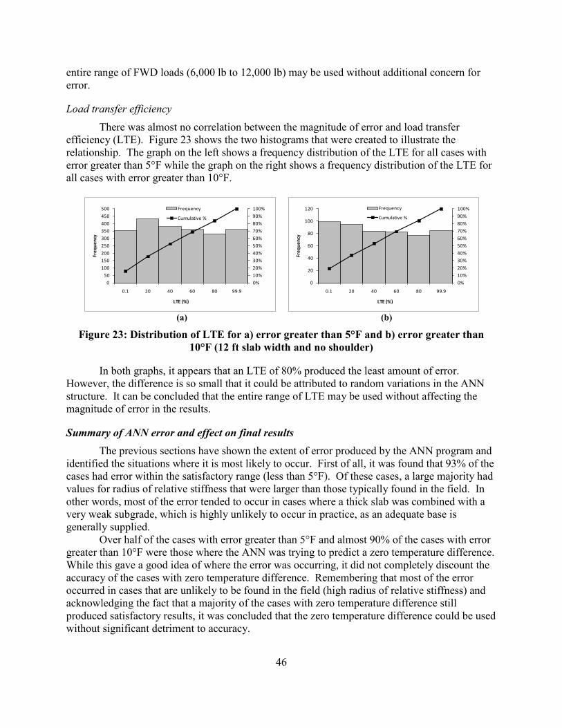
46
entire range of FWD loads (6,000 lb to 12,000 lb) may be used without additional concern for error.
Load transfer efficiency There was almost no correlation between the magnitude of error and load transfer efficiency (LTE). Figure 23 shows the two histograms that were created to illustrate the relationship. The graph on the left shows a frequency distribution of the LTE for all cases with error greater than 5°F while the graph on the right shows a frequency distribution of the LTE for all cases with error greater than 10°F.
(a) (b)
Figure 23: Distribution of LTE for a) error greater than 5°F and b) error greater than 10°F (12 ft slab width and no shoulder)
0%
10%
20%
30%
40%
50%
60%
70%
80%
90%
100%
0
50
100
150
200
250
300
350
400
450
500
0.1 20 40 60 80 99.9
Freq
uenc
y
LTE (%)
Frequency
Cumulative %
In both graphs, it appears that an LTE of 80% produced the least amount of error. However, the difference is so small that it could be attributed to random variations in the ANN structure. It can be concluded that the entire range of LTE may be used without affecting the magnitude of error in the results.
Summary of ANN error and effect on final results The previous sections have shown the extent of error produced by the ANN program and identified the situations where it is most likely to occur. First of all, it was found that 93% of the cases had error within the satisfactory range (less than 5°F). Of these cases, a large majority had values for radius of relative stiffness that were larger than those typically found in the field. In other words, most of the error tended to occur in cases where a thick slab was combined with a very weak subgrade, which is highly unlikely to occur in practice, as an adequate base is generally supplied. Over half of the cases with error greater than 5°F and almost 90% of the cases with error greater than 10°F were those where the ANN was trying to predict a zero temperature difference. While this gave a good idea of where the error was occurring, it did not completely discount the accuracy of the cases with zero temperature difference. Remembering that most of the error occurred in cases that are unlikely to be found in the field (high radius of relative stiffness) and acknowledging the fact that a majority of the cases with zero temperature difference still produced satisfactory results, it was concluded that the zero temperature difference could be used without significant detriment to accuracy.
0%
10%
20%
30%
40%
50%
60%
70%
80%
90%
100%
0
20
40
60
80
100
120
0.1 20 40 60 80 99.9Fr
eque
ncy
LTE (%)
Frequency
Cumulative %

47
A few of the independent variables (coefficient of thermal expansion, joint spacing, and modulus of elasticity) were found to have a moderate correlation with error, but the effects were not great enough to throw the results into question. The variables FWD load and load transfer efficiency were found to have little or no correlation with error. Upon examination of the results presented in this section, it was concluded that the ANN was capable of generating the desired outcome with sufficient accuracy.
Instructions for program installation and use This project shell integrates the generated neural network DLL (macro) with Excel data
through the use of Visual Basic for Applications. A different Excel file is used for each slab length and shoulder type combination. Note that for this program to work, Macros must be enabled.
Before running the program, the file path in the program code must be changed to match that of the DLL and Best Weights files that were included with this spreadsheet. To do this, open the Visual Basic Editor by clicking on the "View" tab, then in the "Macros" pull-down menu, click "View Macros".
Figure 24: Excel screenshot to view macros
A window will pop up. Select the “Width…” Macro and click edit.
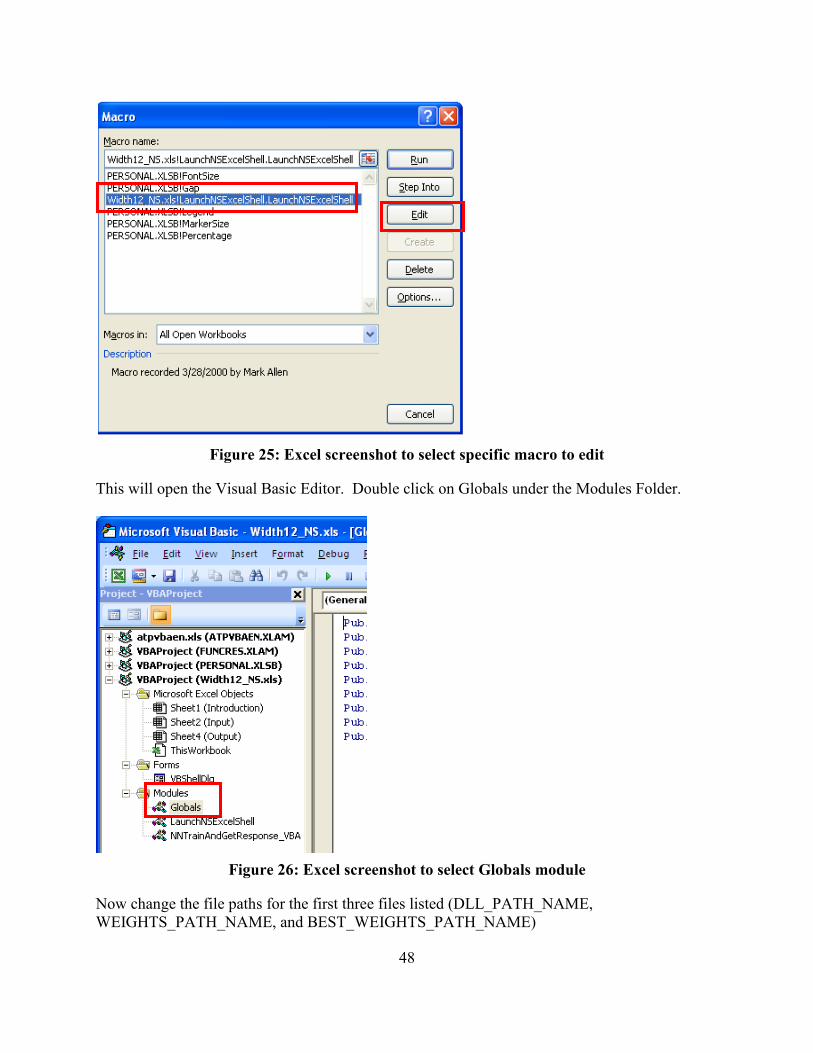
48
Figure 25: Excel screenshot to select specific macro to edit
This will open the Visual Basic Editor. Double click on Globals under the Modules Folder.
Figure 26: Excel screenshot to select Globals module
Now change the file paths for the first three files listed (DLL_PATH_NAME, WEIGHTS_PATH_NAME, and BEST_WEIGHTS_PATH_NAME)
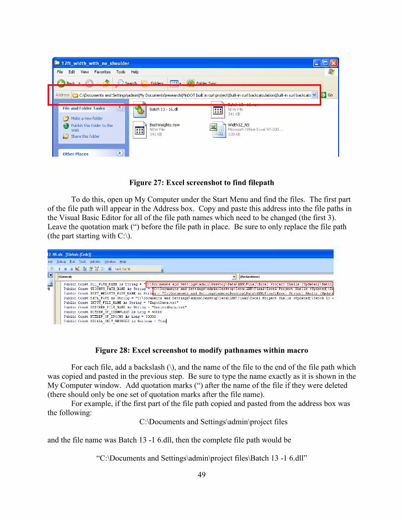
49
Figure 27: Excel screenshot to find filepath
To do this, open up My Computer under the Start Menu and find the files. The first part of the file path will appear in the Address box. Copy and paste this address into the file paths in the Visual Basic Editor for all of the file path names which need to be changed (the first 3). Leave the quotation mark (“) before the file path in place. Be sure to only replace the file path (the part starting with C:\).
Figure 28: Excel screenshot to modify pathnames within macro
For each file, add a backslash (\), and the name of the file to the end of the file path which was copied and pasted in the previous step. Be sure to type the name exactly as it is shown in the My Computer window. Add quotation marks (“) after the name of the file if they were deleted (there should only be one set of quotation marks after the file name).
For example, if the first part of the file path copied and pasted from the address box was the following:
C:\Documents and Settings\admin\project files
and the file name was Batch 13 -1 6.dll, then the complete file path would be
“C:\Documents and Settings\admin\project files\Batch 13 -1 6.dll”

50
The file path for the DATA_PATH file also needs to be changed in the same manner, but the file is likely in another location. Follow the same procedure of finding the file in My Computer, copying the file path from the address bar, pasting into the Visual Basic Editor, and adding the file name to the end. Be sure there are still quotation marks around the entire file path.
Figure 29: Excel screenshot to modify data path within macro
The Visual Basic Editor can now be closed. To run the program in Excel, FWD data and pavement section properties need to be inputted into the 'Input' worksheet. Then, click the 'Run Program' button on the Introduction worksheet to bring up the Custom Solution Wizard window.
Click the 'Get Network Output' button to generate values for temperature gradient using the previously-trained neural network.
Figure 30: Excel screenshot run EBITD ANN
The 'Output' worksheet will receive the output values generated by the DLL. These values can then be compared with measured temperature gradients from thermocouple data at the time of FWD testing to determine the built-in curl.
ANN sample run An example run using FWD data and the ANN is given below. The required inputs are
slab length, FWD load, modulus of subgrade reaction, load transfer efficiency between the slab in question and adjacent slabs, modulus of elasticity and coefficient of thermal expansion of the concrete, slab thickness, and the deflection at the corner from the FWD test. The slab width and restraint conditions are used to select the appropriate ANN batch. In this case, the 12 foot width,
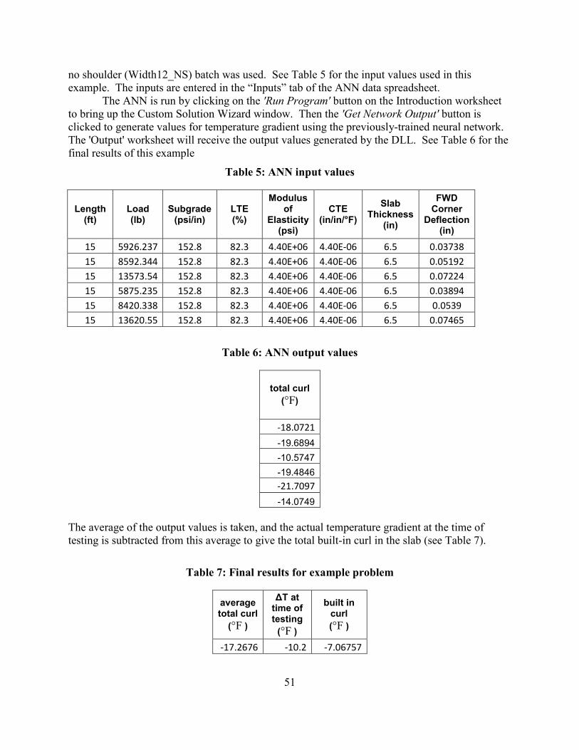
51
no shoulder (Width12_NS) batch was used. See Table 5 for the input values used in this example. The inputs are entered in the “Inputs” tab of the ANN data spreadsheet.
The ANN is run by clicking on the 'Run Program' button on the Introduction worksheet to bring up the Custom Solution Wizard window. Then the 'Get Network Output' button is clicked to generate values for temperature gradient using the previously-trained neural network. The 'Output' worksheet will receive the output values generated by the DLL. See Table 6 for the final results of this example
Table 5: ANN input values
Length (ft)
Load (lb)
Subgrade (psi/in)
LTE (%)
Modulus of
Elasticity (psi)
CTE (in/in/°F)
Slab Thickness
(in)
FWD Corner
Deflection (in)
15 5926.237 152.8 82.3 4.40E+06 4.40E-06 6.5 0.03738 15 8592.344 152.8 82.3 4.40E+06 4.40E-06 6.5 0.05192 15 13573.54 152.8 82.3 4.40E+06 4.40E-06 6.5 0.07224 15 5875.235 152.8 82.3 4.40E+06 4.40E-06 6.5 0.03894 15 8420.338 152.8 82.3 4.40E+06 4.40E-06 6.5 0.0539 15 13620.55 152.8 82.3 4.40E+06 4.40E-06 6.5 0.07465
Table 6: ANN output values
total curl (°F)
-18.0721
-19.6894 -10.5747 -19.4846 -21.7097
-14.0749 The average of the output values is taken, and the actual temperature gradient at the time of testing is subtracted from this average to give the total built-in curl in the slab (see Table 7).
Table 7: Final results for example problem
average total curl
(°F )
ΔT at time of testing
(°F )
built in curl (°F )
-17.2676 -10.2 -7.06757

52
TASKS 3 AND 4: COMPARISON TO OTHER METHODS FOR DETERMINING BUILT-IN CURL AND ASSESSMENT OF VARIABLES
AFFECTING BUILT-IN CURL
Introduction Built-in curl is often quantified by the equivalent temperature gradient needed to deform
a flat slab to the same shape as the curled slab. There are two schools of thought regarding the ideal way to measure the amount of curl built into a concrete slab. A surface profiler can be used to measure the deflections along the length of the slab. This can be accomplished through a variety of different methods including dipsticking, on-site profilometers, high-speed profilometers, etc., which each present their own benefits and drawbacks. These surface profiles can then be plotted and an equation fitted to the shape of the surface. This equation is compared to curves generated using a FEM program (such as ISLAB2000) representing the deflected shape of a theoretical flat slab of the same geometry and properties that is exposed to various temperature gradients. The temperature gradient used to produce the same deflected shape as that of the observed slab is the built-in temperature gradient. This brute force procedure is time consuming and error prone, but does not require specialized techniques or equipment.
Alternately, a falling weight deflectometer (FWD) can be used to measure the response of a pavement to various applied loads. The data obtained from this test can be run through an artificial neural network (ANN), which has been designed and trained to back estimate the built-in curl from Task 2 of this study. This method is much more automated and therefore, the potential to introduce human error is greatly reduced. However, it does require that the user have an appropriately trained ANN at their disposal, as well as access to FWD data at specific times of the day (total negative curl in the slab must be more severe than -10°F).
In this study, several instrumented test slabs at the Minnesota Road Research Facility (MnROAD) were measured with an on-site profilometer (ALPS2) and tested with an FWD. Temperature data for these slabs was obtained from thermal couples imbedded in the slabs. Both methods discussed above were used to estimate the built-in curl of the slabs as defined in Task 3 of this study. The deflection curves obtained from the profilometer were compared to curves for 21 different temperature gradients (from -70°F to 30°F in 5°F increments) generated using ISLAB2000. The FWD data was run through the ANN developed in Task 2 of this study. A third method was also used where the deflected shape measured by the surface profiler was matched with the deflected shapes generated in ISLAB2000 for slabs exposed to various temperature gradients. In this case, the actual profile was matched with the ISLAB2000 profile for which the sum of the squares of the errors between the actual profile and the ISLAB2000 profile was minimized.
Data collection Data was collected at the MnROAD facility, from both the mainline and low volume
loops. For each cell, five transverse profiles were collected, along with FWD deflection data at a variety of locations on the slab. Appendix B of this report shows maps of test patterns of the collected profilometer and FWD data. Thermocouple data provided by Mn/DOT was used to determine the temperature profile through the depth of the slab at the time of both profilometer and FWD testing.
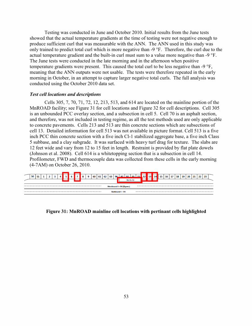
53
Testing was conducted in June and October 2010. Initial results from the June tests showed that the actual temperature gradients at the time of testing were not negative enough to produce sufficient curl that was measurable with the ANN. The ANN used in this study was only trained to predict total curl which is more negative than -9 °F. Therefore, the curl due to the actual temperature gradient and the built-in curl must sum to a value more negative than -9 °F. The June tests were conducted in the late morning and in the afternoon when positive temperature gradients were present. This caused the total curl to be less negative than -9 °F, meaning that the ANN outputs were not usable. The tests were therefore repeated in the early morning in October, in an attempt to capture larger negative total curls. The full analysis was conducted using the October 2010 data set.
Test cell locations and descriptions Cells 305, 7, 70, 71, 72, 12, 213, 513, and 614 are located on the mainline portion of the
MnROAD facility; see Figure 31 for cell locations and Figure 32 for cell descriptions. Cell 305 is an unbounded PCC overlay section, and a subsection in cell 5. Cell 70 is an asphalt section, and therefore, was not included in testing regime, as all the test methods used are only applicable to concrete pavements. Cells 213 and 513 are thin concrete sections which are subsections of cell 13. Detailed information for cell 513 was not available in picture format. Cell 513 is a five inch PCC thin concrete section with a five inch Cl-1 stabilized aggregate base, a five inch Class 5 subbase, and a clay subgrade. It was surfaced with heavy turf drag for texture. The slabs are 12 feet wide and vary from 12 to 15 feet in length. Restraint is provided by flat plate dowels (Johnson et al. 2008). Cell 614 is a whitetopping section that is a subsection in cell 14. Profilometer, FWD and thermocouple data was collected from these cells in the early morning (4-7AM) on October 26, 2010.
Figure 31: MnROAD mainline cell locations with pertinant cells highlighted

54
Figure 32: Mainline cell descriptions from (Mn/DOT 2010)
Cells 36, 37, and 53 are located on the low volume road portion of the MnROAD facility; see Figure 33 for cell locations and Figure 34 for cell descriptions. Cell 36 was subdivided into panels 19 and 20, while cell 37 was subdivided into panels 8 and 9. Profilometer, FWD and thermocouple data was collected from these cells in the early morning (4-7 AM) and late morning (10:30-11:30 AM) on October 26, 2010.
Figure 33: MnROAD low volume road with pertinent cells highlighted from (Mn/DOT 2010)
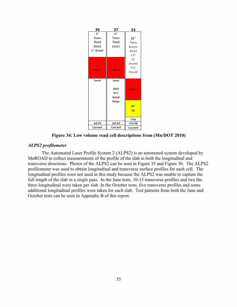
55
Figure 34: Low volume road cell descriptions from (Mn/DOT 2010)
ALPS2 profilometer The Automated Laser Profile System 2 (ALPS2) is an automated system developed by
MnROAD to collect measurements of the profile of the slab in both the longitudinal and transverse directions. Photos of the ALPS2 can be seen in Figure 35 and Figure 36. The ALPS2 profilometer was used to obtain longitudinal and transverse surface profiles for each cell. The longitudinal profiles were not used in this study because the ALPS2 was unable to capture the full length of the slab in a single pass. In the June tests, 10-15 transverse profiles and two the three longitudinal were taken per slab. In the October tests, five transverse profiles and some additional longitudinal profiles were taken for each slab. Test patterns from both the June and October tests can be seen in Appendix B of this report.
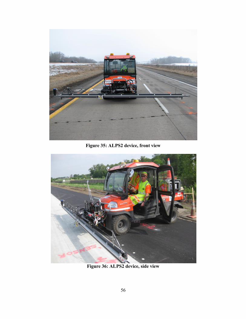
56
Figure 35: ALPS2 device, front view
Figure 36: ALPS2 device, side view
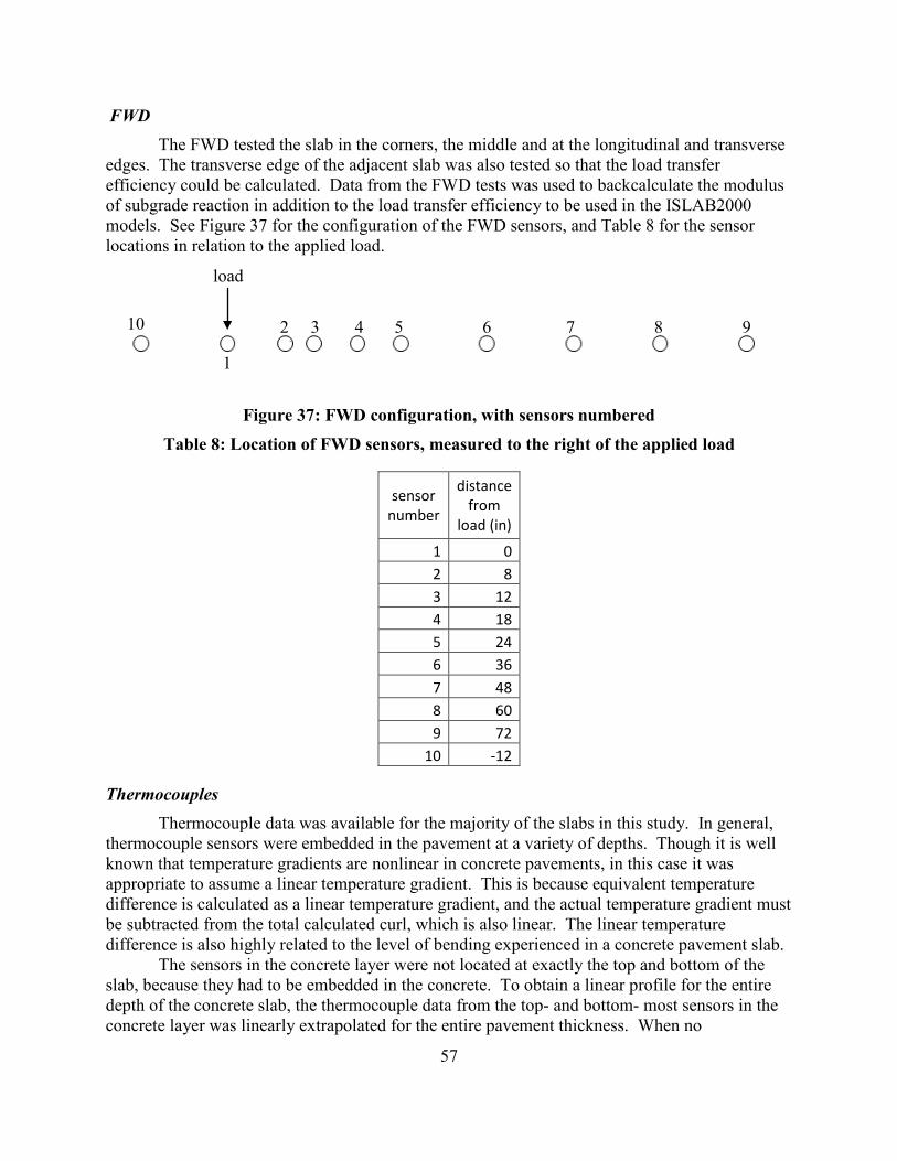
57
FWD The FWD tested the slab in the corners, the middle and at the longitudinal and transverse
edges. The transverse edge of the adjacent slab was also tested so that the load transfer efficiency could be calculated. Data from the FWD tests was used to backcalculate the modulus of subgrade reaction in addition to the load transfer efficiency to be used in the ISLAB2000 models. See Figure 37 for the configuration of the FWD sensors, and Table 8 for the sensor locations in relation to the applied load.
Figure 37: FWD configuration, with sensors numbered
Table 8: Location of FWD sensors, measured to the right of the applied load
sensor number
distance from
load (in)
1 0 2 8 3 12 4 18 5 24 6 36 7 48 8 60 9 72
10 -12
Thermocouples Thermocouple data was available for the majority of the slabs in this study. In general,
thermocouple sensors were embedded in the pavement at a variety of depths. Though it is well known that temperature gradients are nonlinear in concrete pavements, in this case it was appropriate to assume a linear temperature gradient. This is because equivalent temperature difference is calculated as a linear temperature gradient, and the actual temperature gradient must be subtracted from the total calculated curl, which is also linear. The linear temperature difference is also highly related to the level of bending experienced in a concrete pavement slab.
The sensors in the concrete layer were not located at exactly the top and bottom of the slab, because they had to be embedded in the concrete. To obtain a linear profile for the entire depth of the concrete slab, the thermocouple data from the top- and bottom- most sensors in the concrete layer was linearly extrapolated for the entire pavement thickness. When no
load
10 2 3 4 5 6 7 8 9 4
1
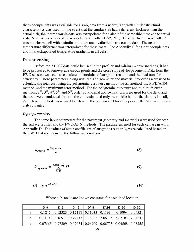
58
thermocouple data was available for a slab, data from a nearby slab with similar structural characteristics was used. In the event that the similar slab had a different thickness than the actual slab, the thermocouple data was extrapolated for a slab of the same thickness as the actual slab. No thermocouple data was available for cells 71, 72, 213, 513, 614. In all cases, cell 12 was the closest cell with a similar structure and available thermocouple data. The actual temperature difference was interpolated for these cases. See Appendix C for thermocouple data and final extrapolated temperature gradients in all cells.
Data processing Before the ALPS2 data could be used in the profiler and minimum error methods, it had
to be processed to remove extraneous points and the cross slope of the pavement. Data from the FWD sensors was used to calculate the modulus of subgrade reaction and the load transfer efficiency. These parameters, along with the slab geometry and material properties were used to calculate the total curl using the polynomial curvature method, the Δh method, the FWD/ANN method, and the minimum error method. For the polynomial curvature and minimum error methods, 2nd, 3rd, 4th, 5th, and 6th, order polynomial approximations were used for the data, and the tests were conducted for both the entire slab and only the middle half of the slab. All in all, 22 different methods were used to calculate the built-in curl for each pass of the ALPS2 on every slab evaluated.
Input parameters The same input parameters for the pavement geometry and materials were used for both
the surface profiler and the FWD/ANN methods. The parameters used for each cell are given in Appendix D. The values of static coefficient of subgrade reaction k, were calculated based on the FWD test results using the following equations:
𝒌𝒔𝒕𝒂𝒕𝒊𝒄 = 𝒌𝒅𝒚𝒏𝒂𝒎𝒊𝒄𝟐
(8)
𝒌𝒊𝒅𝒚𝒏𝒂𝒎𝒊𝒄 = 𝑳𝒐𝒂𝒅∗ 𝑫𝒊∗
𝑫𝒊𝟏𝟎𝟎𝟎
𝓵𝟐 (9)
𝑫𝒊∗ = 𝒂𝒊𝒆−𝒃𝒊𝒆
−𝒄𝒊𝓵 (10)
Where a, b, and c are known constants for each load location,
D*0 D*8 D*12 D*18 D*24 D*36 D*60 a 0.1245 0.12323 0.12188 0.11933 0.11634 0.1096 0.09521 b 0.14707 0.46911 0.79432 1.38363 2.06115 3.62187 7.41241 c 0.07565 0.07209 0.07074 0.06909 0.06775 0.06568 0.06255

59
𝓵 = �𝐥𝐧�𝟔𝟎−𝑨𝒓𝒆𝒂𝟐𝟖𝟗.𝟕𝟎𝟖 �
−.𝟔𝟗𝟖� (11)
𝑫𝟖 𝑫𝟏𝟐 𝑫𝟏𝟖 𝑫𝟐𝟒 𝑫𝟑𝟔 𝑫𝟔𝟎 (12)
𝟐.𝟓𝟔𝟔
𝑨𝒓𝒆𝒂 = 𝟒 + 𝟔 �𝑫𝟎� + 𝟓�
𝑫𝟎� + 𝟔 �
𝑫𝟎� + 𝟗�
𝑫𝟎� + 𝟏𝟖 �
𝑫𝟎� + 𝟏𝟐�
𝑫𝟎�
The load transfer efficiency (LTE) for longitudinal joints was assumed to be 60% for all cases. The LTE for transverse joints was taken as an average of the LTE calculated from the tests before and after the joint, which were found using the formulas below.
𝑳𝑻𝑬𝒋𝒐𝒊𝒏𝒕 𝒃𝒆𝒇𝒐𝒓𝒆 𝑫𝟏 (13)
𝑫𝟑 (14)
= 𝑫𝟏𝟎
𝑳𝑻𝑬𝒋𝒐𝒊𝒏𝒕 𝒂𝒇𝒕𝒆𝒓 =𝑫𝟏
The thickness of the slab was taken as the given thickness for all cases except those noted below. In all cases, the contribution from unbound base layers was ignored. For the thin concrete section (cell 213 & 513), which had slab thicknesses of less than 6 inches, a PCC thickness of 6 inches was used in the FWD/ANN computations since the ANN is not configured for slabs less than 6 inches thick. For the unbonded overlay section (cell 305), an equivalent thickness (Khazanovich 1994) was computed using various configurations to account for the multiple layers. The configuration which gave an equivalent thickness which could be used to compute the most realistic values of the static modulus of subgrade reaction was selected. For PCC layers bonded to a stabilized base (cell 305), the transformed section thickness was calculated based on the following equations.
𝒉𝒆𝒒𝒖𝒊𝒗 𝒑𝒄𝒄𝒑𝒄𝒄
𝒃𝒂𝒔𝒆
+ 𝟏𝟐��𝒙 −𝒉𝒑𝒄𝒄𝟐�𝟐
𝒉𝒑𝒄𝒄 +𝑬𝒃𝒂𝒔𝒆𝑬𝒑𝒄𝒄
�𝒉𝒑𝒄𝒄 − 𝒙 +𝒉𝒃𝒂𝒔𝒆𝟐
�𝟐
𝒉𝒃𝒂𝒔𝒆��
𝟏𝟑
(15)
𝑬𝒑𝒄𝒄𝒉𝒑𝒄𝒄
𝒉𝒑𝒄𝒄𝟐 + 𝑬𝒑𝒄𝒄�𝒉𝒑𝒄𝒄+
𝒉𝒃𝒂𝒔𝒆𝟐 �
𝑬𝒑𝒄𝒄𝒉𝒑𝒄𝒄+𝑬𝒃𝒂𝒔𝒆𝒉𝒃𝒂𝒔𝒆 (16)
= ��𝒉 𝟑 +𝑬𝒃𝒂𝒔𝒆𝑬
𝒉 𝟑�
𝒙 =
Surface profiler The surface profiler data was plotted using Excel to make graphs of deflection versus
point number, see Figure 38. Since the profiler was wider than the slab, there was a certain amount of data on either side of the slab which needed to be deleted. By manually examining the surface profile graphs, the points which required deletion were determined to be those at the
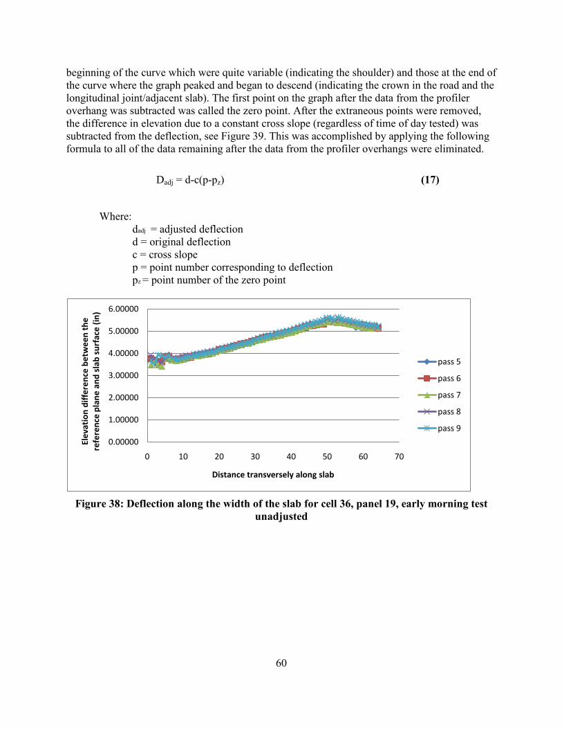
60
beginning of the curve which were quite variable (indicating the shoulder) and those at the end of the curve where the graph peaked and began to descend (indicating the crown in the road and the longitudinal joint/adjacent slab). The first point on the graph after the data from the profiler overhang was subtracted was called the zero point. After the extraneous points were removed, the difference in elevation due to a constant cross slope (regardless of time of day tested) was subtracted from the deflection, see Figure 39. This was accomplished by applying the following formula to all of the data remaining after the data from the profiler overhangs were eliminated.
Dadj = d-c(p-pz) (17)
Where: dadj = adjusted deflection
d = original deflection c = cross slope p = point number corresponding to deflection pz = point number of the zero point
Figure 38: Deflection along the width of the slab for cell 36, panel 19, early morning test
unadjusted
0.00000
1.00000
2.00000
3.00000
4.00000
5.00000
6.00000
0 10 20 30 40 50 60 70
Elev
atio
n di
ffer
ence
bet
wee
n th
e re
fere
nce
plan
e an
d sl
ab s
urfa
ce (i
n)
Distance transversely along slab
pass 5
pass 6
pass 7
pass 8
pass 9
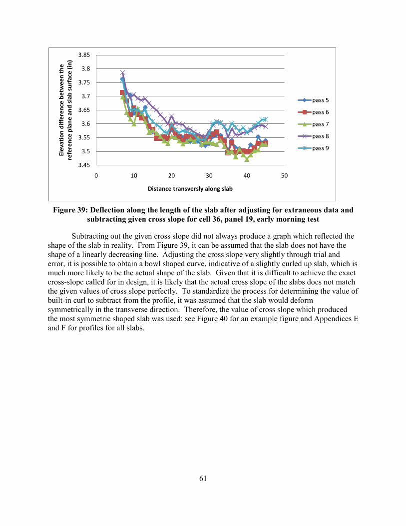
61
Figure 39: Deflection along the length of the slab after adjusting for extraneous data and
subtracting given cross slope for cell 36, panel 19, early morning test
3.45
3.5
3.55
3.6
3.65
3.7
3.75
3.8
3.85
0 10 20 30 40 50
Elev
atio
n di
ffer
ence
bet
wee
n th
e re
fere
nce
plan
e an
d sl
ab s
urfa
ce (i
n)
Distance transversly along slab
pass 5
pass 6
pass 7
pass 8
pass 9
Subtracting out the given cross slope did not always produce a graph which reflected the shape of the slab in reality. From Figure 39, it can be assumed that the slab does not have the shape of a linearly decreasing line. Adjusting the cross slope very slightly through trial and error, it is possible to obtain a bowl shaped curve, indicative of a slightly curled up slab, which is much more likely to be the actual shape of the slab. Given that it is difficult to achieve the exact cross-slope called for in design, it is likely that the actual cross slope of the slabs does not match the given values of cross slope perfectly. To standardize the process for determining the value of built-in curl to subtract from the profile, it was assumed that the slab would deform symmetrically in the transverse direction. Therefore, the value of cross slope which produced the most symmetric shaped slab was used; see Figure 40 for an example figure and Appendices E and F for profiles for all slabs.

62
Figure 40: Deflection along the length of the slab after adjusting for extraneous data and
subtracting assumed cross slope for cell 36, panel 19, early morning test
3.55
3.6
3.65
3.7
3.75
3.8
3.85
0 10 20 30 40 50
Elev
atio
n di
ffer
ence
bet
wee
n re
fere
nce
plan
e an
d sl
ab s
urfa
ce (i
n)
Distance transversly along slab
pass 5
pass 6
pass 7
pass 8
pass 9
This procedure did not affect the calculated values of built-in curl for any of the polynomial curvature methods used except the Δh method, which was dependant on the slope of the profile, see Appendix G for calculations made using both the given and assumed cross slopes for both of these methods. It should be noted that the scales on the abscissa and the ordinate of the deflection curve are not in the same units, and therefore the curvature of the slab is greatly exaggerated.
Polynomial curvature methods The adjusted data was plotted against point number and best fit with polynomial curves
of order two through six were determined using linear algebra. The forms of these polynomials are given in Equations 18 – 22.
Second order: αx2 + βx + γ (18)
Third order: αx3 + βx2 + γx + δ (19)
Fourth order: αx4 + βx3 + γx2 + δx + ε (20)
Fifth order: αx5 + βx4 + γx3 + δx2 + εx + ζ (21)
Sixth order: αx6 + βx5 + γx4 + δx3 + εx2 + ζx + η (22)
A constant curvature (κ) of the best fit polynomial was calculated for each curve by taking the second derivative. For example, the curvature of the second order polynomial was constant at κ = 2α. For larger order polynomials where the curvature is dependent on distance
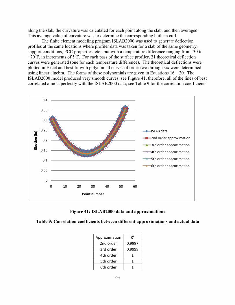
63
along the slab, the curvature was calculated for each point along the slab, and then averaged. This average value of curvature was to determine the corresponding built-in curl.
The finite element modeling program ISLAB2000 was used to generate deflection profiles at the same locations where profiler data was taken for a slab of the same geometry, support conditions, PCC properties, etc., but with a temperature difference ranging from -30 to +700F, in increments of 50F. For each pass of the surface profiler, 21 theoretical deflection curves were generated (one for each temperature difference). The theoretical deflections were plotted in Excel and best fit with polynomial curves of order two through six were determined using linear algebra. The forms of these polynomials are given in Equations 16 – 20. The ISLAB2000 model produced very smooth curves, see Figure 41, therefore, all of the lines of best correlated almost perfectly with the ISLAB2000 data; see Table 9 for the correlation coefficients.
Figure 41: ISLAB2000 data and approximations
0
0.05
0.1
0.15
0.2
0.25
0.3
0.35
0.4
0 10 20 30 40 50 60
Elev
tion
(in)
Point number
ISLAB data
2nd order approximation
3rd order approximation
4th order approximation
5th order approximation
6th order approximation
Table 9: Correlation coefficients between different approximations and actual data
Approximation R2
2nd order 0.9997 3rd order 0.9998 4th order 1 5th order 1 6th order 1

64
The curvature of each best fit polynomial was determined by taking the second derivative of the polynomial. The curvature of each deflection curve on the actual slab was matched up with the 21 theoretical curves for each polynomial order to determine the temperature difference required to produce the observed defections. This process was repeated for each profiler pass on the slab. To automate this process in order to reduce error and human bias, a built-in feature in Excel was used to return the temperature gradient associated with the slab whose curvature most closely matched that of the actual slab. The values of temperature required to produce the observed shape for each pass on the slab were then averaged. It should be noted that the values of curvature obtained for each method were the same, regardless of whether the given or assumed cross slope was used. This is because adjusting the cross slope essentially shifts the data, but does not change the curvature of the curve (see Appendix G for calculations made according to both methods).
For the higher order polynomials (mainly fifth and sixth order), there were occasions when none of the theoretical curvatures closely matched the actual curvature. In these instances, the program returned a value of “#N/A”. Because no value could be determined, the built-in curl was not calculated using the polynomial which produced the error. Manually determining the temperature gradient for which the curvature of the theoretical slab most closely matched that of the actual slab, it was found that generally the temperature gradient was -70°F for these higher order polynomials.
The actual temperature difference at the time of profiler testing was obtained from thermocouple sensors imbedded in the slab. Because no sensors were available at the very top and bottom of the slab, linear extrapolation was used to determine the temperature difference across the entire slab thickness. For slabs where no thermocouple data was available, data from a nearby cell with a similar structure was used.
The value of built-in curl is equal to the total curl less the actual temperature difference.
TBIC = Treq – Tact (23)
Where: TBIC = amount of curl built-in to the slab Treq = average temperature difference required to deform theoretical slab to observed profile
Tact = actual temperature difference across the entire thickness of the field slab at the time of testing
This entire procedure was then repeated using only the middle half of the actual slab, and the middle half of the ISLAB2000 model slabs. Many of the slabs used in this study were restrained at the edges with dowels and ties, and all experienced some restraint due to friction at the joints with other slabs and/or shoulders. The motivation behind discarding a quarter of the length of a pass on either end was the thought that the slabs may deform more symmetrically in the middle, where the edge restraint would have less of an effect. See Appendix H for calculations made for the half-slabs.

65
Δh method In addition to determining the total curl based on polynomial lines of best fit, another
method was used whereby the height differential between the midpoint of the slab and the edges along each pass were compared between the profiled slab and the 21 theoretical slabs subjected to temperature gradients. The profiles generated by ISLAB2000 for the polynomial curvature methods were used in the Δh method. The same Excel program used in the polynomial curvature method was used to find the temperature gradient required to produce the same amount of differential deflection between the middle and the corners of the theoretical slab as in the actual slab. The temperature gradient required to achieve the same differential deflections in the theoretically flat slab as in the actual slab is computed for each pass, and these values are averaged to find the total curl in the slab. It should be noted that using the given cross slopes to create the profiles from which the height differential between the midpoint and the edge of the slab was determined caused unrealistic values of Δh because the resulting profile is linear (see Figure 39). Using the assumed cross-slope to generate the profile (see Figure 40) yields meaningful results for Δh.
Once the total curl in the slab was determined, Equation 21 was used to find the amount of curl built in to the slab, just as in the polynomial curvature method. In this case, Treq is the temperature difference required to obtain the same differential deflections in the theoretically flat slab as in the actual slab.
Minimum error method The minimum error method matched the deflected shape measured by the surface profiler
with the deflected shapes generated in ISLAB2000 for slabs exposed to various temperature gradients. The same ISLAB2000 profiles and the line of best fit for the actual profiles used in the polynomial curvature method were used in the minimum error method. The actual profile was matched with the ISLAB2000 profile for which the sum of the squares of the errors between the line of best fit for the actual profile and the ISLAB2000 profile was minimized. The ISLAB2000 profiles were superimposed on the line of best fit such that midpoints had the same elevation.
This method removed any inherent error in the polynomial curvature method due to curvature calculations by simply matching shapes, not curvatures. Figure 42 shows the second order approximation of the actual data (blue dotted line), and the associated ISLAB2000 profiles (smooth curves) for the same slab exposed to 21 different temperature gradients.
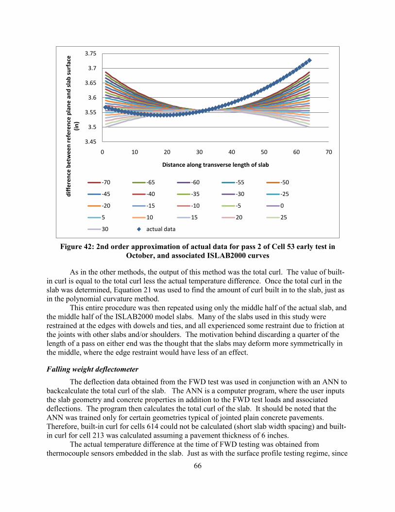
66
3.45
3.5
3.55
3.6
3.65
3.7
3.75
0 10 20 30 40 50 60 70
diff
eren
ce b
etw
een
refe
renc
e pl
ane
and
slab
sur
face
(in
)
Distance along transverse length of slab
-70 -65 -60 -55 -50
-45 -40 -35 -30 -25
-20 -15 -10 -5 0
5 10 15 20 25
30 actual data
Figure 42: 2nd order approximation of actual data for pass 2 of Cell 53 early test in October, and associated ISLAB2000 curves
As in the other methods, the output of this method was the total curl. The value of built-in curl is equal to the total curl less the actual temperature difference. Once the total curl in the slab was determined, Equation 21 was used to find the amount of curl built in to the slab, just as in the polynomial curvature method. This entire procedure was then repeated using only the middle half of the actual slab, and the middle half of the ISLAB2000 model slabs. Many of the slabs used in this study were restrained at the edges with dowels and ties, and all experienced some restraint due to friction at the joints with other slabs and/or shoulders. The motivation behind discarding a quarter of the length of a pass on either end was the thought that the slabs may deform more symmetrically in the middle, where the edge restraint would have less of an effect.
Falling weight deflectometer The deflection data obtained from the FWD test was used in conjunction with an ANN to
backcalculate the total curl of the slab. The ANN is a computer program, where the user inputs the slab geometry and concrete properties in addition to the FWD test loads and associated deflections. The program then calculates the total curl of the slab. It should be noted that the ANN was trained only for certain geometries typical of jointed plain concrete pavements. Therefore, built-in curl for cells 614 could not be calculated (short slab width spacing) and built-in curl for cell 213 was calculated assuming a pavement thickness of 6 inches.
The actual temperature difference at the time of FWD testing was obtained from thermocouple sensors embedded in the slab. Just as with the surface profile testing regime, since

67
no sensors were available at the very top and bottom of the slab, linear extrapolation was used to determine the temperature difference across the entire slab thickness.
The value of built-in curl is equal to the total curl less the actual temperature difference.
TBIC = TANN – Tact (24)
Where: TBIC = amount of curl built-in to the slab TANN = total equivalent temperature difference calculated by the ANN Tact = actual temperature difference across the entire thickness of the slab at the time of testing
The ANN only provides meaningful results for slabs with a total curl more extreme than -9 degrees F. If the ANN yields a total curl of less than -9 degrees F (i.e. the total curl is a small negative number or a positive number), then the curl is either extremely small, positive, or nonexistent.
Results The amount of built-in curl for each test slab was back estimated using the surface
profiler/finite element method for whole and half slabs, the FWD/ANN method, and the minimum error method for whole and half slabs. The results for these tests, after accounting for the actual temperature difference in the slabs, are presented below. A full analysis of the surface profile data using the polynomial curvature, Δh, and minimum error methods was only conducted on the October test data. The FWD/ANN method was run for both the October and June test data.
Table 10 shows the built-in curl calculated via the various polynomial curvature methods for the full slab profiles.

68
Table 10: Built-in curl calculated via the polynomial curvature and Δh methods using full slabs
Built-in Curl (°F)
cell panel time Δ h
method 2nd
order 3rd
order 4th
order 5th
order 6th
order
7 14 early -41.21 -33.21 6.79 #N/A -63.21 #N/A
12 19 early 13.9 -56.1 11.9 #N/A -59.1 #N/A 36 19 early -45.8 -50.8 15.2 -45.8 -59.8 -59.8 36 19 late -76.1 -54.1 -27.1 -76.1 #N/A N/A 36 20 early -47.8 -43.8 15.2 #N/A #N/A #N/A
36 20 late -76.1 -76.1 -31.1 -76.1 #N/A -76.1 37 8 early -59.6 -58.6 21.4 #N/A #N/A #N/A 37 8 late -66.8 -79.8 -14.8 -79.8 #N/A #N/A 37 9 early -59.6 -54.6 20.4 #N/A #N/A #N/A
37 9 late -79.8 -79.8 -15.8 -79.8 #N/A #N/A 53 3 early -48.6 #N/A 18.4 #N/A #N/A #N/A 53 3 late -77.0 #N/A -3.0 -77.0 #N/A -72.0
71* 11 early -50.7 -59.7 15.3 #N/A -59.7 3.3
72* 27 early -60.0 -60.0 10.0 -30.0 #N/A #N/A 213* 15 early -60.2 -66.2 7.8 #N/A #N/A -66.2 305 23 early -63.7 -63.7 6.3 #N/A #N/A -31.7
513* 5 early -66.2 -66.2 3.8 -3.2 #N/A -66.2
614* 57 early -65.2 -60.2 -5.2 #N/A #N/A -66.2 * Thermo-couple data was not available for this cell; instead, data from cell 12 was used.
Table 11 shows the built-in curl calculated with the same polynomial curvature methods, though only considering the middle half of the slab, and discarding the profile measurements taken from the first and last quarter of the transverse width of the slab. Note that the Δh method was not applicable to the analysis of the middle half of the slabs. Full results for each pass for all polynomials for both the whole and half slabs can be seen in Appendices G and H.

69
Table 11: Built-in curl calculated via the polynomial curvature and Δh methods using middle half slabs
Built-in Curl (°F)
cell panel time 2nd
order 3rd
order 4th
order 5th
order 6th
order
7 14 early -63.21 -63.21 10.79 #N/A #N/A
12 19 early -59.07 16.93 #N/A -59.07 #N/A 36 19 early -15.8 8.2 -34.8 #N/A #N/A 36 19 late -76.12 -30.12 -75.12 #N/A N/A 36 20 early -25.8 -10.2 #N/A #N/A #N/A
36 20 late -76.12 -40.12 -76.12 -76.12 -76.12 37 8 early #N/A 15.43 -6.57 #N/A -45.57 37 8 late -59.75 -28.75 #N/A #N/A #N/A 37 9 early 3.43 17.43 #N/A #N/A #N/A
37 9 late -79.75 -27.75 #N/A -79.75 #N/A 53 3 early #N/A 16.37 #N/A #N/A #N/A 53 3 late #N/A -7.03 #N/A #N/A #N/A
71* 11 early -49.71 22.29 #N/A #N/A -49.71
72* 27 early -60.01 9.99 #N/A #N/A #N/A 213* 15 early -62.22 0.78 -66.22 #N/A -64.22 305 23 early -63.71 5.29 -33.71 -63.71 -63.71
513* 5 early -60.22 -4.22 -66.22 #N/A -66.22
614* 57 early -49.22 -20.22 -66.22 3.782519 -66.22 * Thermo-couple data was not available for this cell; instead, data from cell 12 was used.
Table 12 and Table 13 show the built-in curl calculated using the FWD/ANN method based on the June and October test data respectively. It should be noted that, as the ANN can only reliably calculate the curl in slabs with a total curl more negative than -9° F, none of the results from the June test can be considered valid, and only the results for cell 36 panel 20 early and cell 305 from the October test should be considered valid. The cells for which the ANN results are invalid are shown in gray in Table 12 and Table 13.
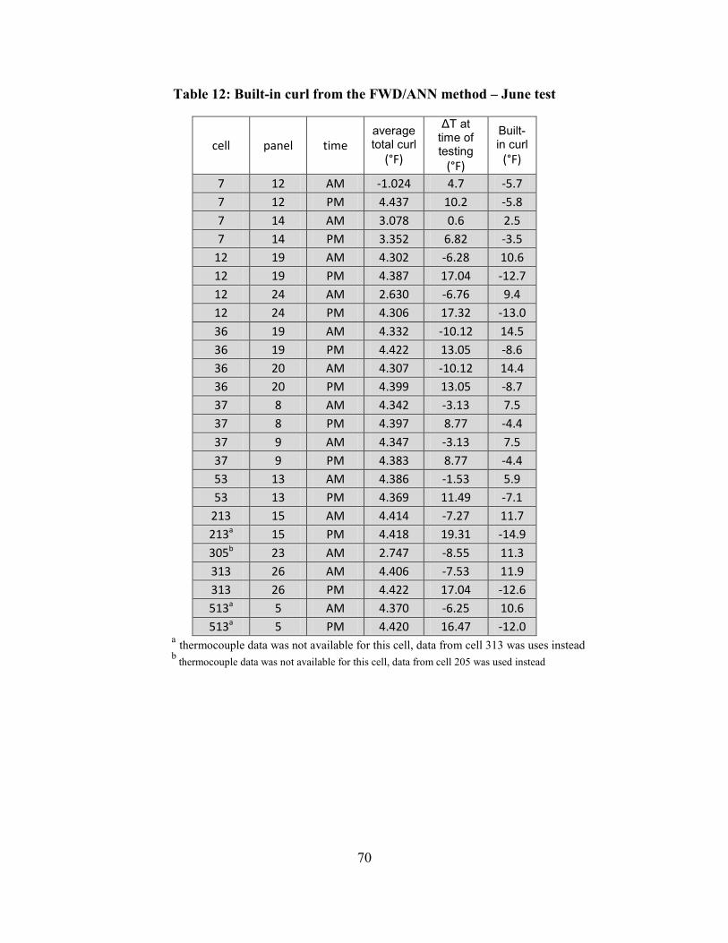
70
Table 12: Built-in curl from the FWD/ANN method – June test
cell panel time average total curl
(°F)
ΔT at time of testing
(°F)
Built-in curl
(°F)
7 12 AM -1.024 4.7 -5.7 7 12 PM 4.437 10.2 -5.8 7 14 AM 3.078 0.6 2.5 7 14 PM 3.352 6.82 -3.5
12 19 AM 4.302 -6.28 10.6 12 19 PM 4.387 17.04 -12.7 12 24 AM 2.630 -6.76 9.4 12 24 PM 4.306 17.32 -13.0 36 19 AM 4.332 -10.12 14.5 36 19 PM 4.422 13.05 -8.6 36 20 AM 4.307 -10.12 14.4 36 20 PM 4.399 13.05 -8.7 37 8 AM 4.342 -3.13 7.5 37 8 PM 4.397 8.77 -4.4 37 9 AM 4.347 -3.13 7.5 37 9 PM 4.383 8.77 -4.4 53 13 AM 4.386 -1.53 5.9 53 13 PM 4.369 11.49 -7.1
213 15 AM 4.414 -7.27 11.7 213a 15 PM 4.418 19.31 -14.9 305b 23 AM 2.747 -8.55 11.3 313 26 AM 4.406 -7.53 11.9 313 26 PM 4.422 17.04 -12.6 513a 5 AM 4.370 -6.25 10.6 513a 5 PM 4.420 16.47 -12.0
a thermocouple data was not available for this cell, data from cell 313 was uses instead b thermocouple data was not available for this cell, data from cell 205 was used instead

71
Table 13: Built-in curl from FWD/ANN method – October test
cell panel time average total curl
(°F)
ΔT at time of testing
(°F)
built in curl (°F)
7 14 early 2.8 -7.1 9.9 12 19 early 2.6 -9.7 12.2
36 19 early 2.8 -10.2 13.0 36 19 late 4.4 5.7 -1.3 36 20 early -10.7 -10.2 -0.5 36 20 late 4.1 5.7 -1.6
37 8 early 4.2 -9.1 13.3 37 8 late 4.3 12.0 -7.7 37 9 early -0.8 -9.1 8.2 37 9 late 4.4 12.0 -7.7
53 3 early 2.3 -15.1 17.4 53 3 late 2.9 10.3 -7.4
71* 11 early 3.4 -10.0 13.4 72* 27 early 3.4 -9.4 12.7
213* 15 early 0.2 -3.5 3.8 305 23 early -14.9 -4.2 -10.8
513* 5 early -5.0 -3.5 -1.5 * Thermocouple data was not available for this cell; data from cell 12 was used instead.
Table 14 shows the results of the minimum error method. The final value for built-in curl
was based on the polynomial approximation which gave the least amount of error between the line of best fit of the actual data and the ISLAB2000.

72
Table 14: Built-in curl determined via the minimum error method for full slabs
Built-in Curl (°F)
cell panel time 2nd
order 3rd
order 4th
order 5th
order 6th
order 7 14 early -48.21 -43.21 -33.21 -3.21 4.29
12 19 early -56.57 -55.32 24.68 10.93 5.93 36 19 early -51.05 -17.3 -56.05 -59.8 -59.8 36 19 late -56.12 -76.12 -76.12 23.88 -1.12 36 20 early -47.3 -11.05 -58.55 -59.8 -59.8 36 20 late -76.12 -76.12 -76.12 -63.62 -76.12 37 8 early -59.57 15.43 -44.57 -13.32 -34.57 37 8 late -79.75 -79.75 -79.75 20.25 -29.75 37 9 early -59.57 24.18 -47.07 6.68 -59.57 37 9 late -79.75 -79.75 -79.75 20.25 -79.75 53 3 early -4.88 -2.38 -27.38 -3.63 -28.63 53 3 late -34.53 -24.53 -77.03 -64.53 -77.03
71* 11 early -59.71 -54.71 -59.71 -59.71 40.29 72* 27 early -60.01 -60.01 -60.01 -60.01 -32.51
213* 15 early -66.22 -66.22 -66.22 -63.72 33.78 305 23 early -65.57 -65.57 -65.57 -65.57 -65.57
513* 5 early -61.22 -63.72 -66.22 -66.22 -16.22 614* 57 early -37.47 -37.47 -37.47 -37.47 31.28
* Thermo-couple data was not available for this cell; instead, data from cell 12 was used.
Table 14 shows the built-in curl calculated via the minimum error method with different order polynomial approximations for the data for the full slab profiles. Table 15 shows the built-in curl calculated with the same method, though only considering the middle half of the slab, and discarding the profile measurements taken from the first and last quarter of the transverse width of the slab. Note that the Δh method was not applicable to the analysis of the middle half of the slabs. Full results for each pass for all polynomials for both the whole and half slabs can be seen in Appendix I.
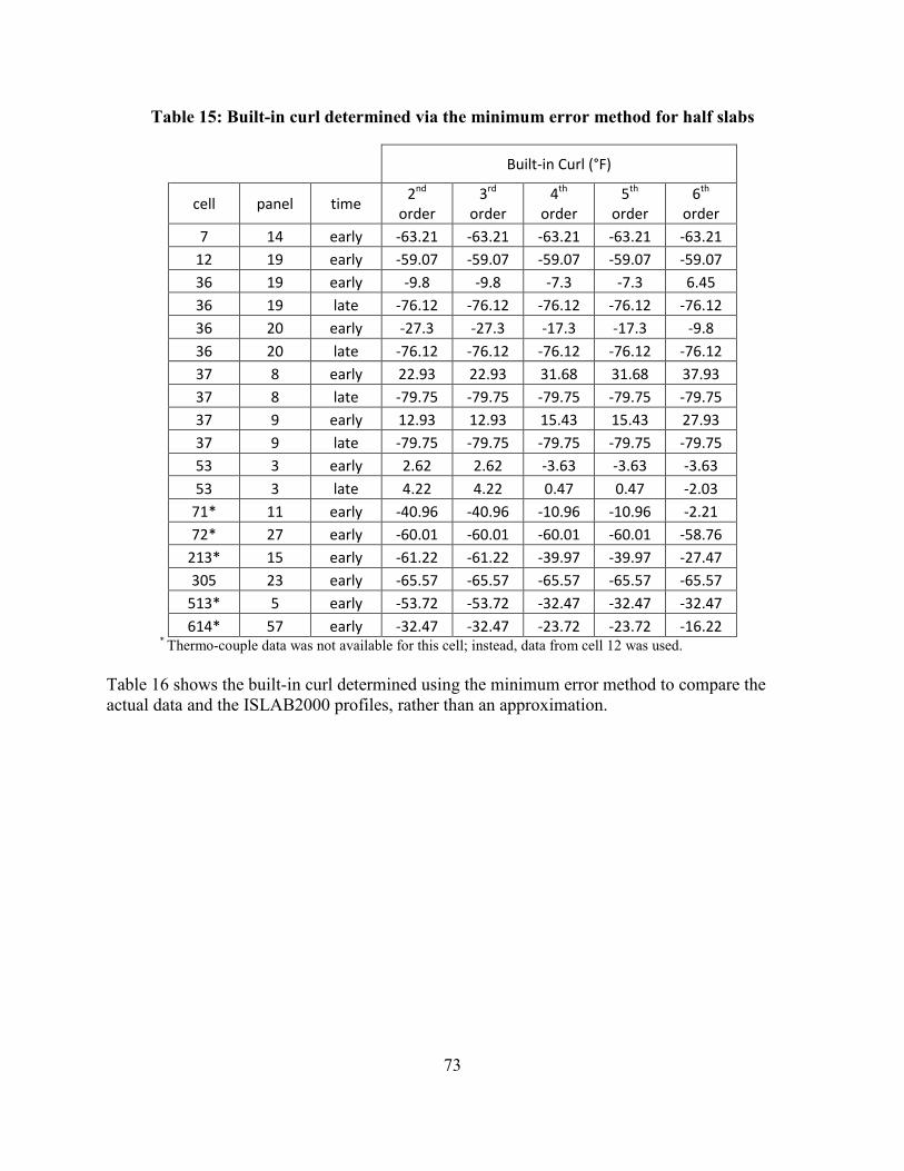
73
Table 15: Built-in curl determined via the minimum error method for half slabs
Built-in Curl (°F)
cell panel time 2nd
order 3rd
order 4th
order 5th
order 6th
order 7 14 early -63.21 -63.21 -63.21 -63.21 -63.21
12 19 early -59.07 -59.07 -59.07 -59.07 -59.07 36 19 early -9.8 -9.8 -7.3 -7.3 6.45 36 19 late -76.12 -76.12 -76.12 -76.12 -76.12 36 20 early -27.3 -27.3 -17.3 -17.3 -9.8 36 20 late -76.12 -76.12 -76.12 -76.12 -76.12 37 8 early 22.93 22.93 31.68 31.68 37.93 37 8 late -79.75 -79.75 -79.75 -79.75 -79.75 37 9 early 12.93 12.93 15.43 15.43 27.93 37 9 late -79.75 -79.75 -79.75 -79.75 -79.75 53 3 early 2.62 2.62 -3.63 -3.63 -3.63 53 3 late 4.22 4.22 0.47 0.47 -2.03
71* 11 early -40.96 -40.96 -10.96 -10.96 -2.21 72* 27 early -60.01 -60.01 -60.01 -60.01 -58.76
213* 15 early -61.22 -61.22 -39.97 -39.97 -27.47 305 23 early -65.57 -65.57 -65.57 -65.57 -65.57
513* 5 early -53.72 -53.72 -32.47 -32.47 -32.47 614* 57 early -32.47 -32.47 -23.72 -23.72 -16.22
* Thermo-couple data was not available for this cell; instead, data from cell 12 was used. Table 16 shows the built-in curl determined using the minimum error method to compare the actual data and the ISLAB2000 profiles, rather than an approximation.

74
Table 16: Built-in curl determined via the minimum error method using actual data and ISLAB2000 profiles
cell panel time Built-in Curl (°F)
7 14 early -63.21 12 19 early -59.07 36 19 early 31.2 36 19 late -76.12 36 20 early -5.8 36 20 late -63.88 37 8 early 26.43 37 8 late -79.75 37 9 early 26.43 37 9 late -70.75 53 3 early 7.37 53 3 late -1.03
71* 11 early -43.71 72* 27 early -59.01
213* 15 early -53.22 305 23 early -65.57
513* 5 early -64.22 614* 57 early -61.22
* Thermo-couple data was not available for this cell; instead, data from cell 12 was used.
Analysis The surface profiler/finite element results were evaluated using the polynomial curvature method, Δh method, and minimum error method. None of these methods consistently gave realistic results; however, as the built-in curl for the slabs investigated is not known, there is no way of determining which method gave the correct value of built-in curl most frequently. Given that these methods did not provide consistent results, they could not be used to verify the FWD/ANN results. The FWD/ANN method is only valid for cells with a total curl more negative than -9° F; in this test, only two cells met this requirement. The values of built-in curl determined by the FWD/ANN for these two cells were both plausible, however, could not be confirmed.
Polynomial curvature and Δh methods The polynomial curvature method calculated values for built-in curl ranging from large
positive to large negative values. Multiple methods of calculating the built-in curl were used in an effort to find a method that would work best. Fitting the data with a quadratic equation is, by far, the most common method for two reasons. First, a curled up slab naturally has a parabolic shape, so the best-fit curve actually has a physical meaning: it is the actual shape of the slab.

75
Second, the derivative of a quadratic is a constant, which makes comparisons between the curvatures of the actual and the theoretical slabs very straightforward.
Characterizing the profile with higher order polynomials may lead to slight increases in the correlation coefficient between the actual profile and the best fit curve. For example, Table 17 shows the correlation coefficient (R2) value for each order polynomial used to best fit the data for Cell 72, pass 3, which is shown in Figure 43.
Table 17: Correlation coefficient (R2) values for various order polynomials for Cell 72, pass 3
order R2
2nd 0.8029 3rd 0.8166 4th 0.8213 5th 0.8224 6th 0.8502
Figure 43: Best-fit polynomals for Cell 72, pass 3
As can be seen in this example, increasing the polynomial order does lead to a slightly better correlation, but the best-fit curve then loses its physical meaning and becomes simply a mathematical model. The one exception to this is that the curvature of the fourth order polynomial is a quadratic and therefore does represent the deflected shape of the slab (Byrum 2000). However, the curvature of a higher order polynomial is dependent on the location along the slab and therefore more computationally intensive. The correlation coefficient was computed between the actual data and each order best fit polynomial for both the transverse pass across the whole slab, and only the middle portion of the slab, see Table 18 and Table 19 respectively. In these tables, the highest correlation coefficient for a particular slab is shaded.
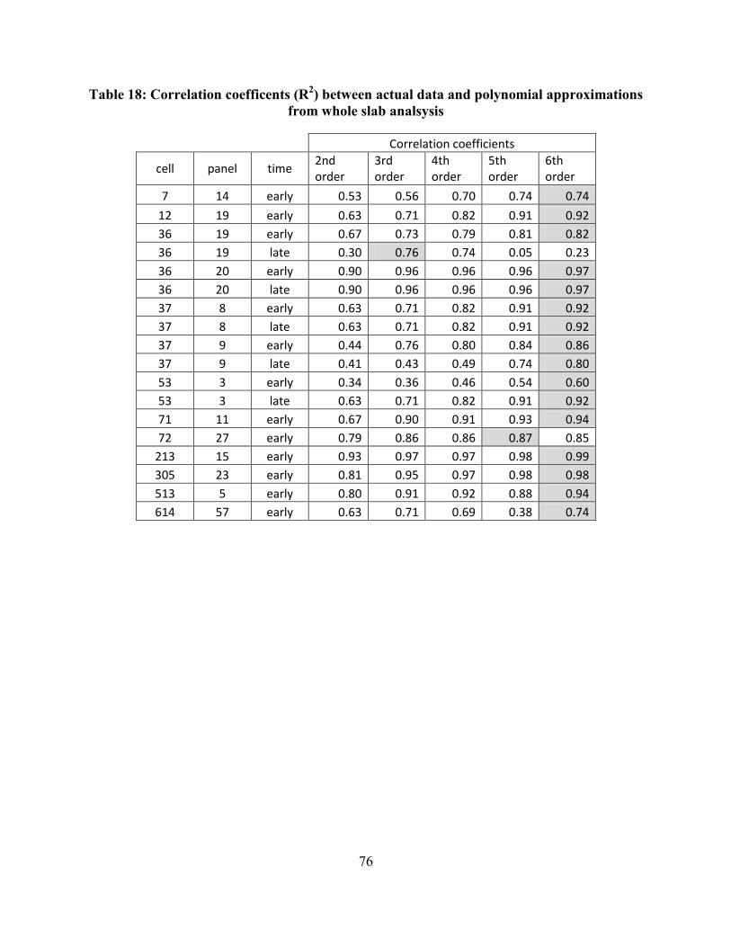
76
Table 18: Correlation coefficents (R2) between actual data and polynomial approximations from whole slab analsysis
Correlation coefficients
cell panel time 2nd order
3rd order
4th order
5th order
6th order
7 14 early 0.53 0.56 0.70 0.74 0.74
12 19 early 0.63 0.71 0.82 0.91 0.92 36 19 early 0.67 0.73 0.79 0.81 0.82 36 19 late 0.30 0.76 0.74 0.05 0.23 36 20 early 0.90 0.96 0.96 0.96 0.97 36 20 late 0.90 0.96 0.96 0.96 0.97 37 8 early 0.63 0.71 0.82 0.91 0.92 37 8 late 0.63 0.71 0.82 0.91 0.92 37 9 early 0.44 0.76 0.80 0.84 0.86 37 9 late 0.41 0.43 0.49 0.74 0.80 53 3 early 0.34 0.36 0.46 0.54 0.60 53 3 late 0.63 0.71 0.82 0.91 0.92 71 11 early 0.67 0.90 0.91 0.93 0.94 72 27 early 0.79 0.86 0.86 0.87 0.85
213 15 early 0.93 0.97 0.97 0.98 0.99 305 23 early 0.81 0.95 0.97 0.98 0.98 513 5 early 0.80 0.91 0.92 0.88 0.94 614 57 early 0.63 0.71 0.69 0.38 0.74
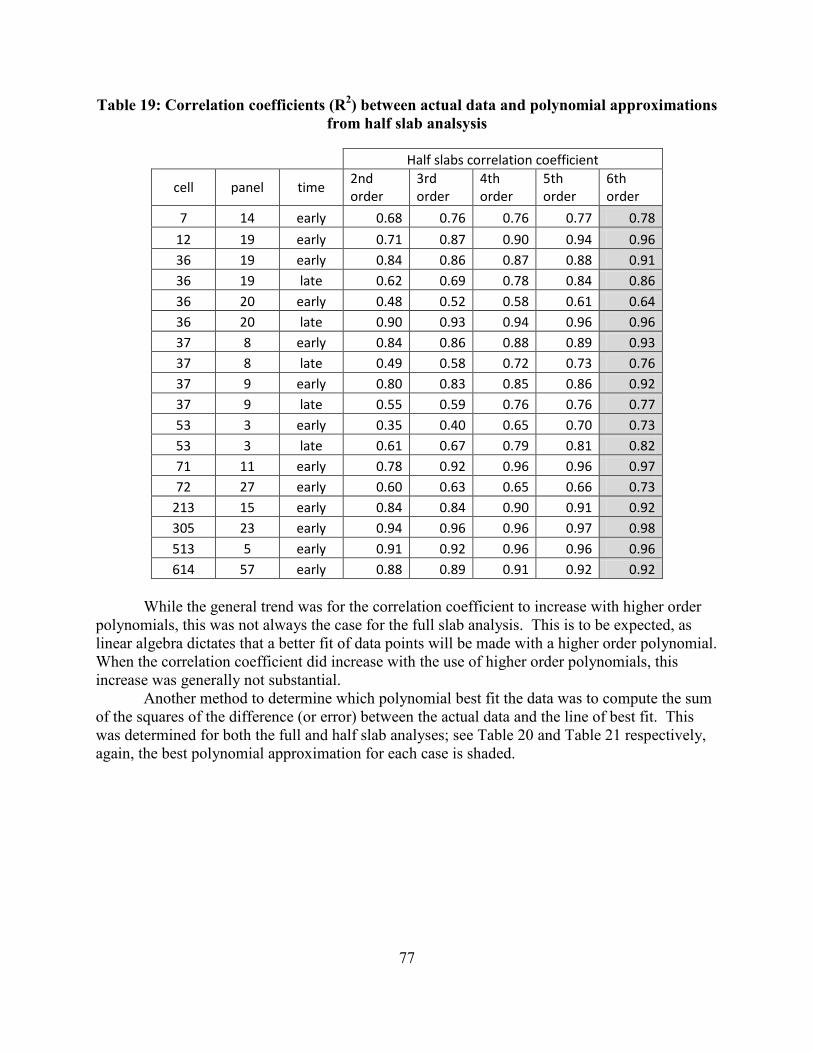
77
Table 19: Correlation coefficients (R2) between actual data and polynomial approximations from half slab analsysis
Half slabs correlation coefficient
cell panel time 2nd order
3rd order
4th order
5th order
6th order
7 14 early 0.68 0.76 0.76 0.77 0.78
12 19 early 0.71 0.87 0.90 0.94 0.96 36 19 early 0.84 0.86 0.87 0.88 0.91 36 19 late 0.62 0.69 0.78 0.84 0.86 36 20 early 0.48 0.52 0.58 0.61 0.64 36 20 late 0.90 0.93 0.94 0.96 0.96 37 8 early 0.84 0.86 0.88 0.89 0.93 37 8 late 0.49 0.58 0.72 0.73 0.76 37 9 early 0.80 0.83 0.85 0.86 0.92 37 9 late 0.55 0.59 0.76 0.76 0.77 53 3 early 0.35 0.40 0.65 0.70 0.73 53 3 late 0.61 0.67 0.79 0.81 0.82 71 11 early 0.78 0.92 0.96 0.96 0.97 72 27 early 0.60 0.63 0.65 0.66 0.73
213 15 early 0.84 0.84 0.90 0.91 0.92 305 23 early 0.94 0.96 0.96 0.97 0.98 513 5 early 0.91 0.92 0.96 0.96 0.96 614 57 early 0.88 0.89 0.91 0.92 0.92
While the general trend was for the correlation coefficient to increase with higher order
polynomials, this was not always the case for the full slab analysis. This is to be expected, as linear algebra dictates that a better fit of data points will be made with a higher order polynomial. When the correlation coefficient did increase with the use of higher order polynomials, this increase was generally not substantial.
Another method to determine which polynomial best fit the data was to compute the sum of the squares of the difference (or error) between the actual data and the line of best fit. This was determined for both the full and half slab analyses; see Table 20 and Table 21 respectively, again, the best polynomial approximation for each case is shaded.
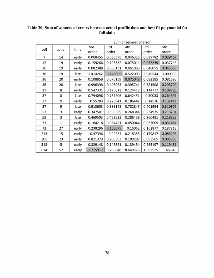
78
Table 20: Sum of squares of errors between actual profile data and best fit polynomial for full slabs
sum of squares of error
cell panel time 2nd order
3rd order
4th order
5th order
6th order
7 14 early 0.068455 0.065575 0.046325 0.039782 0.039467 12 19 early 0.159266 0.123332 0.075014 0.037239 0.037745 36 19 early 0.082388 0.065131 0.051983 0.048055 0.043695
36 19 late 1.414262 0.448095 0.522003 3.949544 3.000933 36 20 early 0.108859 0.076159 0.075048 0.082185 0.081695 36 20 late 0.996398 0.403063 0.395741 0.381508 0.295709 37 8 early 0.547331 0.175613 0.124412 0.114777 0.109796 37 8 late 0.794096 0.767706 0.642451 0.30033 0.264691 37 9 early 0.55283 0.225641 0.186442 0.14536 0.132411 37 9 late 0.913603 0.888148 0.782845 0.401994 0.310879 53 3 early 0.347501 0.330325 0.268344 0.234935 0.215294 53 3 late 0.469503 0.452533 0.286458 0.260481 0.218923 71 11 early 0.184218 0.054421 0.050044 0.037609 0.031481 72 27 early 0.238296 0.160075 0.16062 0.162877 0.187812
213 15 early 0.47396 0.22224 0.218355 0.179817 0.085203 305 23 early 0.821379 0.205393 0.109287 0.093565 0.092965 513 5 early 0.329148 0.146821 0.139454 0.265197 0.119431 614 57 early 1.715912 3.296648 8.649725 15.92525 46.848
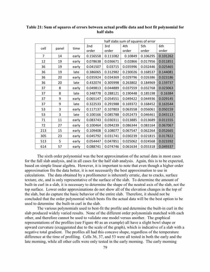
79
Table 21: Sum of squares of errors between actual profile data and best fit polynomial for half slabs
half slabs sum of squares of error
cell panel time 2nd order
3rd order
4th order
5th order
6th order
7 14 early 0.156558 0.111082 0.10849 0.106295 0.101262 12 19 early 0.078638 0.036671 0.02866 0.017956 0.011851 36 19 early 0.041507 0.03715 0.035996 0.032446 0.025465 36 19 late 0.386065 0.312982 0.230026 0.168537 0.144081 36 20 early 0.035924 0.034369 0.029796 0.026386 0.023186 36 20 late 0.432074 0.305998 0.263802 0.184969 0.159737 37 8 early 0.049813 0.044889 0.037559 0.032768 0.023063 37 8 late 0.348778 0.288121 0.190448 0.185198 0.16384 37 9 early 0.065147 0.054551 0.049422 0.044936 0.029145 37 9 late 0.322533 0.291988 0.169372 0.168452 0.163544 53 3 early 0.117137 0.107803 0.063558 0.056061 0.050159 53 3 late 0.100166 0.085788 0.052473 0.046461 0.043113 71 11 early 0.083743 0.030311 0.013885 0.013689 0.011555 72 27 early 0.100464 0.094239 0.086344 0.083164 0.067067
213 15 early 0.109408 0.108077 0.067547 0.062264 0.052665 305 23 early 0.045792 0.031741 0.030239 0.021815 0.017822 513 5 early 0.054447 0.047851 0.025062 0.024568 0.023392 614 57 early 0.088741 0.074746 0.061634 0.055318 0.049337
The sixth order polynomial was the best approximation of the actual data in most cases
for the full slab analysis, and in all cases for the half slab analysis. Again, this is to be expected, based on simple linear algebra. However, it is important to note that even though a higher order approximation fits the data better, it is not necessarily the best approximation to use in calculations. The data obtained by a profilometer is inherently erratic, due to cracks, surface texture, etc, and is only representative of the surface of the slab. To determine the amount of built-in curl in a slab, it is necessary to determine the shape of the neutral axis of the slab, not the top surface. Lower order approximations do not show all of the elevation changes in the top of the slab, but do capture the basic behavior of the entire slab. Therefore, it should not be concluded that the order polynomial which bests fits the actual data will be the best option to be used to determine the built-in curl in the slab.
The various polynomials used to best-fit the profile and determine the built-in curl in the slab produced widely varied results. None of the different order polynomials matched with each other, and therefore cannot be used to validate one model versus another. The graphical representations of the profiles (see Figure 40 as an example) all have a slight bowl shape or upward curvature (exaggerated due to the scale of the graph), which is indicative of a slab with a negative total gradient. The profiles all had this concave shape, regardless of the temperature difference at the time of profiling. Cells 36, 37, and 53 were all tested in both the early and the late morning, while all other cells were only tested in the early morning. The early morning

80
temperature gradients were all negative (i.e. the top of the slab is cooler than the bottom), while in the late morning tests, all of the temperature gradients were positive (i.e. the top is warmer than the bottom). Given that all of the measured profiles had a negative total curl (based on their shape), regardless of the temperature gradient present, it can be concluded that the expected built-in gradient was negative.
The only polynomial which consistently predicted negative built-in curl was the fifth order polynomial. However, the fifth order polynomial was also the most unreliable method which returned a value of “N/A” in 14 cases out of 18. This is likely due to the fact that the fifth order polynomial has no physical meaning, but is merely a line which is closest to the most points in the profile. However, profile data has a large amount of small variations due surface imperfections and therefore matching the largest amount of points does not guarantee a more accurate representation of the shape of the slab. When the fifth order polynomial did produce results, it predicted large negative values of built-in curl, from -23 to -60°F, which are unlikely to be accurate. The sixth order polynomial also returned a value of “N/A” on 10 occasions, and predicted large negative values of built-in curl, as did the second and fourth order polynomials, and the Δh method. The third order polynomial curvature methods gave generally low negative or even positive values of built-in curl. Given that the exact values of curl are not known, it is difficult to states that one method can be declared more accurate than the others.
In an effort to reduce the error caused by edge restraints, the data for the first and last quarter of each pass was discarded, and the remaining data was reanalyzed via the polynomial curvature method. In this analysis, the third order polynomial was the only approximation that consistently produced results; the 4th, 5th, and 6th order approximations all yielded a value of “N/A” for many of the cases and predicted very large values of built-in curl when results were produced. The third order polynomial predicted values of built-in curl that were either positive or less negative than those given by the other methods. Though the values of built-in curl determined from the half slab analysis differed from those calculated in the full slab analysis, the trends in the data were similar.
One way to compare the validity of the various methods is to examine the results given for the same cell tested at different times. In the October round of testing, cells 36, 37, and 53 were all tested in both the early morning (5-7am) and late morning (10-11am). The 2nd order polynomial predicted values of built-in curl which were very similar for the early and late tests for cell 36 using both the polynomial curvature and minimum error methods.
In an effort to determine which order polynomial was most likely to produce accurate results, a statistical analysis was conducted. In this analysis, the sum of the square of the errors between the actual data, and the ISLAB2000 profile which best matched the actual data based on curvature was computed for each order polynomial assumed in the polynomial curvature method. Additionally, the sum of the square of the errors between the line of best fit for the actual data and the ISLAB2000 profile which best matched the actual data based on curvature was computed for each order polynomial assumed in the polynomial curvature method. See Appendix K for these values.
Table 22 shows which order polynomial minimized the sum of the squares of the error. The best option is based on value which minimized the sum of the squares of the errors between the actual data and the ISLAB2000 profile selected based on the profilometer method.
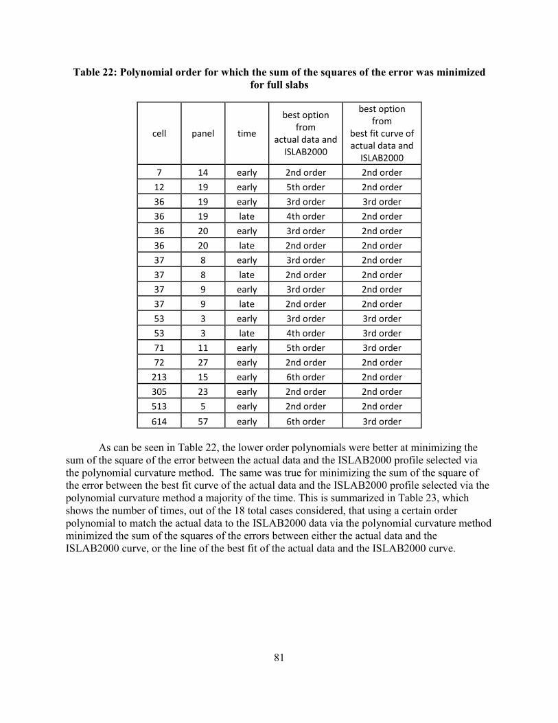
81
Table 22: Polynomial order for which the sum of the squares of the error was minimized for full slabs
cell panel time
best option from
actual data and ISLAB2000
best option from
best fit curve of actual data and
ISLAB2000
7 14 early 2nd order 2nd order
12 19 early 5th order 2nd order
36 19 early 3rd order 3rd order
36 19 late 4th order 2nd order
36 20 early 3rd order 2nd order
36 20 late 2nd order 2nd order
37 8 early 3rd order 2nd order
37 8 late 2nd order 2nd order
37 9 early 3rd order 2nd order
37 9 late 2nd order 2nd order
53 3 early 3rd order 3rd order
53 3 late 4th order 3rd order
71 11 early 5th order 3rd order
72 27 early 2nd order 2nd order
213 15 early 6th order 2nd order
305 23 early 2nd order 2nd order
513 5 early 2nd order 2nd order
614 57 early 6th order 3rd order As can be seen in Table 22, the lower order polynomials were better at minimizing the
sum of the square of the error between the actual data and the ISLAB2000 profile selected via the polynomial curvature method. The same was true for minimizing the sum of the square of the error between the best fit curve of the actual data and the ISLAB2000 profile selected via the polynomial curvature method a majority of the time. This is summarized in Table 23, which shows the number of times, out of the 18 total cases considered, that using a certain order polynomial to match the actual data to the ISLAB2000 data via the polynomial curvature method minimized the sum of the squares of the errors between either the actual data and the ISLAB2000 curve, or the line of the best fit of the actual data and the ISLAB2000 curve.

82
Table 23: Frequency of a polynomial being the best option
polynomial actual data
and ISLAB2000
best fit curve of actual data and
ISLAB2000 2nd order 7 13 3rd order 5 5 4th order 2 0 5th order 2 0 6th order 2 0
As can be seen from Table 23, lower order polynomials, in general, minimized the sum of
the square of the error between the ISLAB2000 profile selected via the polynomial curvature method and either the actual data or the best fit curve of the actual data. This is likely because lower order polynomials “smooth out” the imperfections in the surface profile due to tining, cracks, spalls, etc., and are more representative of the behavior of the entire slab. The ISLAB2000 model does not include distresses or discrepancies in the slab surface; therefore, approximations which produce smoother curves will match the ISLAB2000 models more accurately.
Another way the accuracy of various polynomial approximations used in the polynomial curvature method was investigated was through the analysis using on the profilometer data from the middle half of the slabs. Consistency between the results of the whole and half slab analyses shows that a particular approximation is a good fit for the data. Table 24 shows the number of times that the built-in curl calculated by the polynomial curvature method for the full slabs was within 4°F of that calculated using only data from the middle half of the slab for each order polynomial approximation used. It can be seen that the 2nd, 3rd, and 6th order approximations yielded matches most frequently. However, none of the order polynomial approximations produced at match more than five times out of 18. One reason the 2nd order approximation may have had the most matches between the full and half slab analyses is that the curvature is not dependent on the location along the slab for a quadratic.
Table 24: Number of matches between full and half slab analsyes using the polynomial curvature method
polynomial order
number of matches
2nd 5 3rd 4 4th 2 5th 1 6th 4
The lack of consistency between the full and half slab analyses shows that the polynomial
curvature method is very sensitive to the data profile. The motivation behind the half slab analysis was that restraints and edge effects could distort the ends of the profile. Removing a

83
quarter of the data on either end of the profile would remove these edge effects. However, any gross deviations from the general trend of the profile would have been removed in the data processing phase. Therefore, the half slab analysis removed extra data points which could have been used to better fit a curve, but likely did not increase accuracy from the removal of edge effects.
Since the profiler method is so sensitive to the data profile, it is important to ensure that the data is as accurate as possible. The actual profiler device used to make the measurements, the ALPS2, has a margin of error of approximately +/- 0.015 in, increasing to +/- .025in at the ends of the device. This is a fairly large margin of error, given that the profiler obtains data out to the hundred thousandth of an inch. Adjacent data points often vary by only hundredths or thousandths of an inch, which within the margin of error of the ALPS2.
Another source of error was that several of the slabs in this study had surface defects or discontinuities, such as cracks, spalls, tining and diamond grinding. Cracks function as joints, and change how the pavement slab deforms. The polynomial curvature and Δh methods assume that the slab deforms symmetrically, which is not the case for cracked slabs. Additionally, the profiler measurements are for the slab surface, so any variation in the surface will be shown in the profile.
Figure 44 shows the transverse profile of a slab with some form of discrepancy, cell 37, panel 8, before subtracting the cross slope. Approximately half way across the slab, the profile for each pass has a significant jump. The damage report for this cell indicates that there is not a crack in this location; however, the cell does have strips of diamond grinding, which could account for the discontinuity.
Figure 44: Transverse profile of cracked slab without adjusting for cross slope - cell 37, panel 8, late morning test from October testing
4
4.2
4.4
4.6
4.8
5
5.2
5.4
5.6
5.8
0 10 20 30 40 50 60
Elev
atio
n di
ffer
ence
bet
wee
n th
e re
fere
nce
plan
e an
d sl
ab s
urfa
ce (i
n)
Distance transversly along slab
pass 0
pass 1
pass 2
pass 3
pass 4
Figure 45 shows the same set of data, cell 37 panel 8, after adjusting for the cross slope. It can be seen that this is not a smooth, bowl shaped curve, and the deformations are certainly not symmetrical. This lack of symmetry is important because the ISLAB2000 program used to

84
generate the model slabs to which the actual data was compared does not account for cracks or other discontinuities in the slab.
Figure 45: Transverse profile of cracked slab after adjusting for cross slope - cell 37, panel
8, late morning test from October testing
3.9
3.95
4
4.05
4.1
4.15
4.2
4.25
0 10 20 30 40 50 60
Elev
atio
n di
ffer
ence
bet
wee
n re
fere
nce
plan
e an
d sl
ab s
urfa
ce (i
n)
Distance transversly along slab
pass 0
pass 1
pass 2
pass 3
pass 4
In addition to error in the data collection process, the polynomial curvature method has several sources of inherent error and ample opportunity to introduce inaccuracy through human variability. The transverse profiles from the June test varied in terms of the number of points in a pass and the number of transverse passes per slab; this made it more difficult to automate the data processing procedure. In the October tests, five transverse profiles were taken for each slab. Each profile was the average of three scans in the same location, and contained the exact same number of data points. Receiving the data in a slightly processed format, where every run had the same number of data points was very helpful to automate the processing procedure, and it is recommended that the data always be given in this format. The zero-point is selected quite subjectively by the data processor, as are the extraneous points. The choice of which points to include or exclude greatly influenced the curvature of the best-fit curve, which is used to estimate the total curl. In an effort to reduce this source of error, the same data processor selected which points should be deleted each time. Another source of error is that the FEM model curves were only run in increments of 5° F. Using theoretical deflection curves in one or two degree increments would have increased accuracy, but was computationally too intensive to be feasible. To reduce error in the process of matching up the actual and theoretical deflection curves, a computer program was used, so that the selection criteria were consistent.
Another source of error was that the ISLAB2000 program used to create finite element models of the slabs and generate the deflected shapes for slabs subjected to various temperature gradients assumes a rectangular geometry and cannot account for skewed joints. Therefore, the ISLAB2000 profiles do not reflect the actual geometry of any slabs with skewed joints (cells 7, 36, and 37). Slabs with skewed joints will also not deform symmetrically in the transverse
85
direction; when processing the profilometer data to find the actual profiles, an assumption of symmetrical deformation in the transverse direction was made.
FWD/ANN method The FWD/ANN method did not produce usable values for built-in curl for most cells
tested because the total curl calculated was less negative than -9°F. The ANN used in this study was only trained to predict total curl which is more negative than -9 °F. In an effort to obtain usable results, the test data from the FWD tests conducted in the morning was used because it is likely that the temperature gradient of a slab would be negative. This negative gradient coupled with a negative built-in curl gradient (which is typically found in pavement slabs) was more likely to be a large enough negative value that the ANN would be able to back estimate total curl. The tests conducted in the afternoon, when the actual temperature gradient is positive, would require a very large value of built-in curl before the ANN would be able to accurately estimate the total curl. Indeed, when analysis was conducted on the FWD test data from the afternoon, all results were found to be unusable.
Since many of the values of total curl calculated by the ANN were more positive than -9 °F, it may be concluded that those of the slabs tested have either very low negative, or no built in curl. It could also indicate that the slabs have a positive built-in curl; however, this is highly unlikely, as this condition is very rare for pavements paved under conditions similar to those at MnROAD (wet climate, restraint from initial construction, high negative temperature difference in concrete at final set, etc.). Values of very low or no built-in curl for other MnROAD test slabs are also consistent to those found by Vandenbossche (2003). The ANN could be used to calculate such low values for built-in curl if the actual temperature gradient were great enough such that the total value of built in curl were more negative than -9°F. This is likely to occur in the morning in the fall in Minnesota, and based on this recommendation additional FWD testing was conducted in the fall of 2010.
Previous testing, which occurred in June, was not conducted in the presence of a temperature gradient sufficiently negative to produce usable data for the ANN. Cell 513 and cell 36 panel 20 were tested in June, and the ANN was not able to calculate usable results; for both cells, the ANN returned a total curl of 4 °F. The same slabs were tested in October, and found to have a total curl large enough that the ANN results can be considered valid. Subtracting out the actual temperature difference from the total curl gives very small negative values of built-in curl for both cells, which is consistent with the built-in curl generally found in MnROAD PCC pavements (Vandenbossche 2003).
Though many of the cells did not have a sufficiently negative gradient at the time of testing to obtain an accurate value of built-in curl, the theoretical lower bound on the amount of built-in curl present can be calculated. As discussed previously, the ANN will not return usable values of built-in curl if the total temperature gradient at the time of testing is less negative that -9 °F. Recall that the total temperature gradient is the sum of the actual temperature gradient at the time of testing and the built-in gradient. By assuming that the total gradient is the largest possible value it could be, in this case -9 °F, and subtracting the actual gradient, a theoretical lower limit on amount of built-in curl in the slab was calculated. These values are given in Table 25. For these calculations, only the early morning October tests were used, as these tests had temperature gradients more similar to those with which the ANN was trained.

86
Table 25: Lower bound value of built-in curl
cell panel
ΔT at time of testing (deg F)
Lower limit of built in
curl (deg F)
7 14 -7.1 -1.9 12 19 -9.7 0.7 36 19 -10.2 1.2 37 8 -9.1 0.1 37 9 -9.1 0.1 53 3 -15.1 6.1
71* 11 -10.0 1.0 72* 27 -9.4 0.4
213* 15 -3.5 -5.5 305 23 -4.2 -4.8
513* 5 -3.5 -5.5 614* 57 -3.5 -5.5
* Thermo-couple data was not available for this cell; instead, data from cell 12 was estimated
through interpolation. The lower bound calculated in this manner was generally a small negative or small
positive value. This is consistent with the amount of built-in curl determined for other cells in the MnROAD facility (Vandenbossche 2003).
Minimum error method Similar to the polynomial curvature method, the minimum error method produced quite
varied results. The 5th and 6th order approximations predicted a mix of positive and negative values for built-in curl, while the 2nd, 3rd, and 4th order approximations were generally just negative. For all approximations, if a built-in curl was predicted to be negative, it tended to be a very large negative number.
To determine which polynomial approximation was likely to be the most accurate, the sums of the squares of the errors between the line of best fit of the data and the ISLAB2000 profile were compared. The 2nd order polynomial was by far the best approximation in both the whole and half slab analyses, as can be seen in Table 26. In this table, the best option is the order polynomial of the line of best fit of the actual data for which the sum of the squares of the errors between that line of best fit and the ISLAB2000 approximation was minimized.
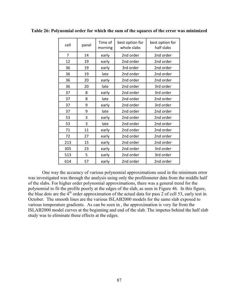
87
Table 26: Polynomial order for which the sum of the squares of the error was minimized
cell panel Time of morning
best option for whole slabs
best option for half slabs
7 14 early 2nd order 2nd order
12 19 early 2nd order 2nd order
36 19 early 3rd order 2nd order
36 19 late 2nd order 2nd order
36 20 early 2nd order 2nd order
36 20 late 2nd order 3rd order
37 8 early 2nd order 3rd order
37 8 late 2nd order 2nd order
37 9 early 2nd order 3rd order
37 9 late 2nd order 2nd order
53 3 early 2nd order 2nd order
53 3 late 2nd order 2nd order
71 11 early 2nd order 2nd order
72 27 early 2nd order 2nd order
213 15 early 2nd order 2nd order
305 23 early 2nd order 3rd order
513 5 early 2nd order 3rd order
614 57 early 2nd order 2nd order
One way the accuracy of various polynomial approximations used in the minimum error was investigated was through the analysis using only the profilometer data from the middle half of the slabs. For higher order polynomial approximations, there was a general trend for the polynomial to fit the profile poorly at the edges of the slab, as seen in Figure 46. In this figure, the blue dots are the 4th order approximation of the actual data for pass 2 of cell 53, early test in October. The smooth lines are the various ISLAB2000 models for the same slab exposed to various temperature gradients. As can be seen in , the approximation is very far from the ISLAB2000 model curves at the beginning and end of the slab. The impetus behind the half slab study was to eliminate these effects at the edges.

88
Figure 46: 4th order polynomial approximation pass 2 of cell 53 early test vs. ISLAB2000
3.4
3.6
3.8
4
4.2
4.4
4.6
4.8
5
5.2
5.4
5.6
0 10 20 30 40 50 60 70
diff
eren
ce b
etw
een
refe
renc
e pl
ane
and
slab
sur
face
(in)
Distance along transverse length of slab
-70 -65 -60 -55 -50-45 -40 -35 -30 -25-20 -15 -10 -5 05 10 15 20 2530 actual data
For consistency between all cases, the first and last quarter of the actual data was discarded (points 0-15, and 49-64). This effectively eliminated the edge effects, as can be seen in Figure 47, which shows the same 4th order approximation for the pass in the same cell as Figure 46, only with the first and last quarter of the approximation discarded. It should be noted that the scale on these figures is different because the outliers were eliminated.
Though the edge effects were removed, for this case, the line of best fit is does not match the ISLAB2000 profiles well. This is eliminated by using a lower order polynomial, such as the quadratic. Figure 48 shows the second order approximation of the same pass in the same cell as Figure 46 and Figure 47. It can be seen in this figure that the second order approximation will match the ISLAB2000 profiles better than the 4th order.
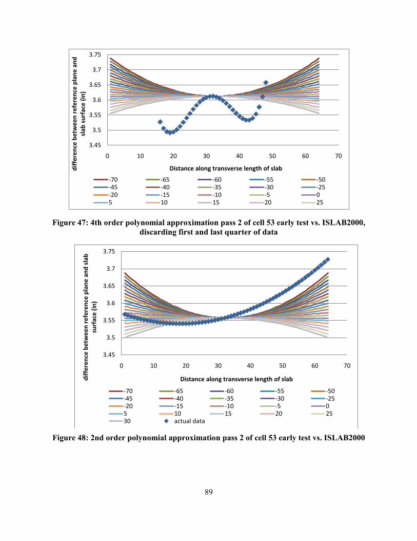
89
Figure 47: 4th order polynomial approximation pass 2 of cell 53 early test vs. ISLAB2000, discarding first and last quarter of data
Figure 48: 2nd order polynomial approximation pass 2 of cell 53 early test vs. ISLAB2000
3.45
3.5
3.55
3.6
3.65
3.7
3.75
0 10 20 30 40 50 60 70
diff
eren
ce b
etw
een
refe
renc
e pl
ane
and
slab
sur
face
(in)
Distance along transverse length of slab
-70 -65 -60 -55 -50-45 -40 -35 -30 -25-20 -15 -10 -5 05 10 15 20 25
3.45
3.5
3.55
3.6
3.65
3.7
3.75
0 10 20 30 40 50 60 70
diff
eren
ce b
etw
een
refe
renc
e pl
ane
and
slab
su
rfac
e (in
)
Distance along transverse length of slab
-70 -65 -60 -55 -50-45 -40 -35 -30 -25-20 -15 -10 -5 05 10 15 20 2530 actual data

90
Consistency between the results of the whole and half slab analyses shows that a particular approximation fits all of the data well, rather than just the middle portion. It does not mean that a particular approximation is best for calculating the built-in curl. Table 27 shows the number of times that the built-in curl calculated by the minimum error method for the full slabs was within 4°F of that calculated using only data from the middle half of the slab for each order polynomial approximation used. No one order polynomial stood out as a better option when compared to the rest, however, the 6th order approximation had the least number of matches between the whole and half slabs.
Table 27: Number of matches for built-in curl between full and half slab analsyes using the minimum error method
polynomial order
number of matches
2nd 6 3rd 8 4th 6 5th 8 6th 3
Compared with the number of matches between the whole and half slab analyses for the
polynomial curvature method (Table 24), the minimum error method shows more consistency. This is likely due to the fact that the minimum error method compared the ISLAB2000 profiles to the line of best fit for the actual data, so many of the imperfections in the measured slab profile did not affect the error calculation as significantly as in the polynomial curvature method.
This was further shown by the additional test performed to determine the built-in curl based on the ISLAB2000 profile which minimized the sum of the square of the errors between the actual data and the ISLAB2000 profiles.
Figure 49 shows the actual data (blue dots) superimposed on the 21 different ISLAB2000 models (smooth lines).

91
Figure 49: Actual data pass 1, cell 72 vs. ISLAB2000
3
3.05
3.1
3.15
3.2
3.25
3.3
0 10 20 30 40 50 60 70
diff
eren
ce b
etw
een
refe
renc
e pl
ane
and
slab
sur
face
(in
)
Distance along transverse length of slab
-70 -65 -60 -55 -50 -45-40 -35 -30 -25 -20 -15-10 -5 0 5 10 1520 25 30 pass 1
As can be seen from this figure, the actual data is inherently very erratic. Additionally this data incorporates surface discrepancies, such as tining and distresses, which do not affect the entire thickness of the slab. The error between the actual data and ISLAB2000 profiles, and the error between polyn
use the data setrently more errmuch lower the
omial approximations and ISLAB2000 profiles were not compared directly beca s contained different numbers of points, which means one dataset would have inhe or than the other. However, it was generally observed that the error per point was comparison between ISLAB2000 and the polynomial approximations than for the comparison between ISLAB2000 and the actual data. This reinforces the concept that the surface profile only captures the profile of the surface, which is not representative of the entire shape, especially if the slab is tined, or has surface defects.
The sources of error in the minimum error method were the same as with polynomial curvature method because they use same profile data, processing techniques and ISLAB2000 models. The only difference in error sources was that the polynomial curvature method depended on the curvature of the line of best fit, and the assumption that the average curvature was representative of the curvature of the slab. The minimum error method eliminated this source of error by directly comparing deformed shapes, rather than curvatures.
Comparison of results from different methods Due to limitations in the ANN discussed above, results were only obtained for cell 305, and the cell 36 panel 20 early test. The value of built-in curl obtained for these cells by any of the profilometer methods does not match with the built-in curl obtained by the ANN. It should be noted that, as none of the profilometer methods were verified, this does not mean that the

92
ANN results are incorrect, just that they cannot be validated. As the expected built-in curl values for this section are quite low (or near zero), this is not completely surprising.
The biggest difference between the polynomial curvature method and the minimum error method was that the polynomial curvature method matched the actual data to an ISLAB2000 model based on curvature, while the minimum error method matched the profiles based on their actual shape. For any polynomial of higher order than a quadratic, curvature is simply a mathematical parameter with no physical meaning in terms of the overall slab shape. For all order polynomials, the minimum error method retains physical meaning.
One major advantage the minimum error method had over the polynomial curvature method was that the minimum error method always produced results. Recall that for the polynomial curvature method, anytime the difference between the curvature of the line of best fit of the actual data and the curvature of the ISLAB2000 profiles was outside of the tolerance of the automated matching program, a value of “N/A” was returned. This was not an issue in the minimum error method because profiles were matched based on the minimum amount of error, rather than on a similarity between two sets of data. However, it should be noted that even though the minimum error method can consistently produce results, this does not mean those results are any more accurate than those from the polynomial curvature method. A comparison of the results of the polynomial curvature method and the minimum error method showed that the value of built-in curl predicted using the 2nd order polynomial approximation are very consistent, particularly for the full slab analysis, as can be seen in Table 28.

93
Table 28: Built-in curl calculated using a second order polynomial approximation in both the polynomial curvature and minimum error methods
cell panel time
Built-in Curl (°F) from the
minimum error method
Built-in Curl (°F) from the polynomial curvature method
percent difference
7 14 early -6.96 -9.21 28% 12 19 early -56.57 -56.07 -1% 36 19 early -51.05 -50.8 0% 36 19 late -56.12 -54.12 -4% 36 20 early -47.3 -43.8 -8% 36 20 late -76.12 -76.12 0% 37 8 early -59.57 -58.57 -2% 37 8 late -79.75 -79.75 0% 37 9 early -59.57 -54.57 -9% 37 9 late -79.75 -79.75 0% 53 3 early -4.88 #N/A N/A 53 3 late -34.53 #N/A N/A 71 11 early -59.71 -59.71 0% 72 27 early -60.01 -60.01 0%
213 15 early -66.22 -66.22 0% 305 23 early -65.57 -63.71 -3% 513 5 early -61.22 -66.22 8% 614 57 early -37.47 -60.22 47%
This consistency was also found, to a lesser extent, for the built-in curl calculated with the 2nd order polynomial approximation in the half slab analysis. No other order polynomial approximation showed consistency between the two methods.
One factor which likely did not affect the results from any of the methods used was the presence of creep. Previous studies have found that after the pavement is more than one year old, creep does not substantially affect the amount of built-in curl (Rao et al. 2001; Schmidt 2001).Since all of the pavements tested were at two years old at the time of testing (Johnson et al. 2008), creep effects most likely did not affect the total curl measured.
Conclusions In this study, cells of PCC pavements at MnROAD were profiled using an ALPS2 profilometer and tested with an FWD. The profile data was plotted and best-fitted with various order polynomial curves in Excel. ISLAB2000 was used to generate similar profiles for a theoretically flat slab of the same composition, subjected to different temperature gradients, and similar equations of best-fit were found. The differential deflection between the middle and edge of the slab profiles were also found for both the actual and theoretical slabs. The curvature and differential deflections of the profiles were compared to find the temperature gradient required to

94
produce the same shape in the theoretical profile as that of the actual slab; this temperature gradient is called the total temperature gradient. The total temperature gradient required to deform the theoretical slab to the actual slab was also determined by finding the theoretical slab profile required to minimize the sum of the squares of the errors between the actual the theoretical slabs. The actual temperature gradient at the time of testing was subtracted from the temperature gradient to find the built-in curl. Data obtained from the FWD tests were run through an ANN to backcalculate the built-in curl of the same slabs. The results obtained from all of the methods tested were compared and the following conclusions were drawn:
• FWD testing must be performed when a large negative total gradient is present to use the current ANN as the sensitivity to corner deflections is minimal at built-in curl level greater than -9°F (close to zero).
• Based on the graphs of the profiles, all cells tested have negative built-in temperature gradients.
• A second order polynomial is the easiest to work with when fitting profiles because the curvature is a constant value. The quadratic equation also gives a physical representation of the shape of the slab.
• A higher order polynomial has no physical meaning, but is merely a line which is closest to the most points in the profile. However, profile data has a large amount of small variation due to cracks and spalls, surface texture, etc, and therefore matching the largest amount of points does not guarantee a more accurate representation of the shape of the slab.
• The second and third order polynomials produced the most realistic values of built-in curl.
• The results from both the polynomial curvature and minimum error methods for the second order polynomial approximation matched fairly well.
• A fifth order polynomial gave the least realistic values of built-in curl and was the most likely to not return a value of built-in curl.
• Automating as much of the process as possible when determining the curvature of the actual profile and the temperature gradient required to deform a flat slab to the same shape as the actual slab reduces errors.
• Receiving the data in a consistent format (ex. always having the same number of points in a pass), allows for increased automation and ease in backcalculating the level of curl in the concrete slabs.
Due to the fact that exact values of curl in the slabs tested are not known, no one method can be declared more accurate than the others. Further testing on slabs of known built-in curl will be required before such a determination can be made.

95
REFERENCES
Altoubat, S. A., and Lange, D. A. (2001). "Creep, Shrinkage, and Cracking of Restrained Concrete at Early Age." ACI Materials Journal, 98(4), 323-331.
Armaghani, J. M., Larsen, T. J., and Smith, L. L. (1987). "Temperature Response of Concrete Pavements." Transportation Research Record, 1121, 23-33.
Beckemeyer, C. A., Khazanovich, L., and Yu, H. T. (2002). "Determining the Amount of Built-in Curling in JPCP: A Case Study of Pennsylvania I-80." Transportation Research Board Annual Meeting, Washington, D.C.
Bissonnette, B., Attiogbe, E. K., Miltenberger, M. A., and Fortin, C. (2007). "Drying Shrinkage, Curling, and Joint Opening of Slabs-on-Ground." ACI Materials Journal, 104(3), 259-267.
Byrum, C. R. (2000). "Analysis by High Speed Profile of Jointed Concrete Pavement Slab Curvatures." Transportation Research Record, 1730, 1-9.
Choubane, B., and Tia, M. (1995). "Analysis and Verification of Thermal-Gradient Effects on Concrete Pavement." Journal of Transportation Engineering, 121(1), 75-81.
Dere, Y., Asgari, A., Sotelino, E. D., and Archer, G. C. (2006). "Failure Prediction of Skewed Jointed Plain Concrete Pavements Using 3D FE Analysis." Engineering Failure Analysis, 13(6), 898-913.
Eisenmann, J., and Leykauf, G. (1990). "Effect of Paving Temperature on Pavement Performance." 2nd International Workshop on the Theoretical Design of Concrete Pavements, Siguenza, Spain, 419-428.
Guo, E. H. (2001). "Back-Estimation of Slab Curling and Joint Stiffness." 7th International Conference on Concrete Pavements, Orlando, FL.
Hansen, W., Smiley, D. L., Peng, Y., and Jensen, E. A. (2002). "Validating Top-Down Premature Transverse Slab Cracking in Jointed Plain Concrete Pavement (JPCP)." Transportation Research Board Annual Meeting, Washington, D.C.
Hansen, W., Wei, Y., Smiley, D. L., Peng, Y., and Jensen, E. A. (2006). "Effects of Paving Conditions on Built-in Curling and Pavement Performance." International Journal of Pavement Engineering, 7(4), 291-296.
Heath, A. C., Roesler, J. R., and Harvey, J. T. (2001). "Quantifying Longitudinal, Corner and Transverse Cracking in Jointed Concrete Pavements." Transportation Research Board Annual Meeting, Washington, D.C.
Ioannides, A. M., Davis, C. M., and Weber, C. M. (1999). "Westergaard Curling Solution Reconsidered." Transportation Research Record, 1684, 61-70.
Ioannides, A. M., and Salsilli-Murua, R. A. (1989). "Temperature Curling in Rigid Pavements: An Application of Dimensional Analysis." Transportation Research Record, 1227, 1-11.
Jahangirnejad, S., Buch, N., and Kravchenko, A. (2009). "Evaluation of Coefficient of Thermal Expansion Test Protocol and Its Impact on Jointed Concrete Pavement Performance." ACI Materials Journal, 106(1), 64-71.
Jeong, J.-H., and Zollinger, D. G. (2004). "Insights on Early-Age Curling and Warping Behavior from a Fully Instrumented Test Slab System." Transportation Research Board Annual Meeting, Washington, D.C.
Johnson, A., Clyne, T. R., and Worel, B. J. (2008). 2008 MnROAD Phase II Construction Report, Minnesota Department of Transportation, St. Paul, MN.

96
Khazanovich, L. (1994). Structural Analysis of Multi-Layered Concrete Pavement Systems. University of Illinois Urbana-Champaign, Urbana, IL.
Khazanovich, L., Selezneva, O. I., Yu, H. T., and Darter, M. I. (2001). "Development of Rapid Solutions for Prediction of Critical Continuously Reinforced Concrete Pavement Stresses." Transportation Research Record, 1778, 64-72.
Lee, Y.-H., and Darter, M. I. (1994). Development of Pavement Prediction Models. University of Illinois, Urbana, IL.
Lim, S., Jeong, J.-H., and Zollinger, D. G. (2004). "Moisture Profiles and Shrinkage in Early-Age Concrete." Transportation Research Board Annual Meeting, Washington, D.C.
Mallela, J., Abbas, A., Harman, T., Rao, C., Liu, R., and Darter, M. I. (2005). "Measurement and Significance of the Coefficient of Thermal Expansion of Concrete in Rigid Pavement Design." Transportation Research Record, 1919, 38-46.
Mn/DOT. (2010). "MnROAD_ML_Cell Maps_August 2010." http://www.dot.state.mn.us/mnroad/testsections/pdfs/MnROAD_ML_Cell%20Maps_August%202010.pdf, M. M. C. M. A. 2010.pdf, ed., Minnesota Department of Transportation, St. Paul, MN. Accessed March 15, 2011.
Papagiannakis, A. T., and Masad, E. A. (2008). Pavement Design and Materials. John Wiley & Sons, Inc., Hoboken, NJ.
Poblete, M., Salsilli, R., Valenzuela, R., Bull, A., and Spratz, P. (1988). "Field Evaluation of Thermal Deformations in Undoweled PCC Pavement Slabs." Transportation Research Record, 1207, 217-227.
Rao, C., Barenberg, E. J., Snyder, M. B., and Schmidt, S. (2001). "Effects of Temperature and Moisture on the Response of Jointed Concrete Pavements." 7th International Conference on Concrete Pavements, Orlando, FL.
Rao, S., and Roesler, J. R. (2005a). "Characterizing Effective Built-In Curling from Concrete Pavement Field Measurements." Journal of Transportation Engineering, 131(4), 320-327.
Rao, S., and Roesler, J. R. (2005b). "Nondestructive Testing of Concrete Pavements for Characterization of Effective Built-In Curling." Journal of Testing and Evaluation, 33(5), 1-8.
Rao, S. P. (2005). "Characterizing Effective Built-In Curling and Its Effect on Concrete Pavement Curling." Dissertation, University of Illinois at Urbana-Champaign, Urbana, IL.
Reddy, A. S., Leonards, G. A., and Harr, M. E. "Warping Stresses and Deflections in Concrete Pavements: Part III." Highway Research Board Proceedings, 1-24.
Schmidt, S. K. (2001). Analysis of "Built-In" Curling and Warping in PCC Pavements. University of Minnesota, Minneapolis, MN.
Sondag, S. K., and Snyder, M. B. (2003). "Analysis of 'Built-in' Curling and Warping of PCC Pavements." 6th International DUT Workshop on Fundamental Modelling of Design and Performance of Concrete Pavements, Old-Turnhout, Belgium.
Tang, T., Zollinger, D. G., and Senadheera, S. (1993). "Analysis of Concave Curling in Concrete Slabs." Journal of Transportation Engineering, 119(4), 618-633.
Vandenbossche, J. M. (2003). "Interpreting Falling Weight Deflectometer Results for Curled and Warped Portland Cement Concrete Pavements." Thesis, University of Minnesota, Minneapolis, MN.

97
Vandenbossche, J. M. (2007). "Effects of Slab Temperature Profiles on Use of Falling Weight Deflectometer Data to Monitor Joint Performance and Detect Voids." Transportation Research Record, 2005, 75-85.
Wells, S. A., Phillips, B. M., and Vandenbossche, J. M. (2006a). "Characterizing Strain Induced by Environmental Loads in Jointed Plain Concrete Pavements." Transportation Research Record, 1947, 36-48.
Wells, S. A., Phillips, B. M., and Vandenbossche, J. M. (2006b). "Quantifying Built-in Construction Gradients and Early-age Slab Deformation Caused by Environmental Loads in a Jointed Plain Concrete Pavement." International Journal of Pavement Engineering, 7(4), 275-289.
www.curvefitting.com. (2009). "DataFit Version 9.0." Accessed 2009. www.dynatest.com. (2009). "Dynatest." Accessed 2009. www.nd.com. (2009). "NeuroDimension." Accessed 2009. Yu, H. T., and Khazanovich, L. (2001). "Effects of Construction Curling on Concrete Pavement
Behavior." 7th International Conference on Concrete Pavements, Orlando, FL. Yu, H. T., Khazanovich, L., Darter, M. I., and Ardani, A. (1998). "Analysis of Concrete
Pavement Responses to Temperature and Wheel Loads Measured from Instrumented Slabs." Transportation Research Record, 1639, 94-101.

APPENDIX A: ERROR REPORTS
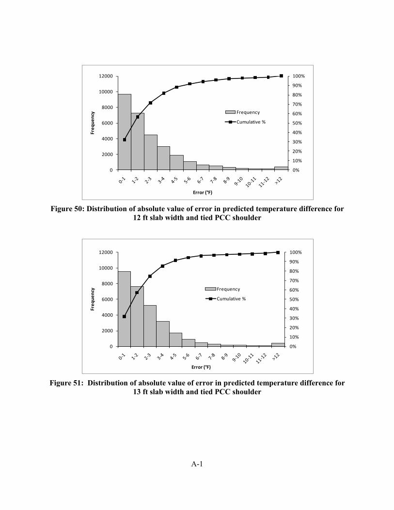
A-1
0%
10%
20%
30%
40%
50%
60%
70%
80%
90%
100%
0
2000
4000
6000
8000
10000
12000
Freq
uenc
y
Error (°F)
Frequency
Cumulative %
Figure 50: Distribution of absolute value of error in predicted temperature difference for
12 ft slab width and tied PCC shoulder
Figure 51: Distribution of absolute value of error in predicted temperature difference for
13 ft slab width and tied PCC shoulder
0%
10%
20%
30%
40%
50%
60%
70%
80%
90%
100%
0
2000
4000
6000
8000
10000
12000
Freq
uenc
y
Error (°F)
Frequency
Cumulative %
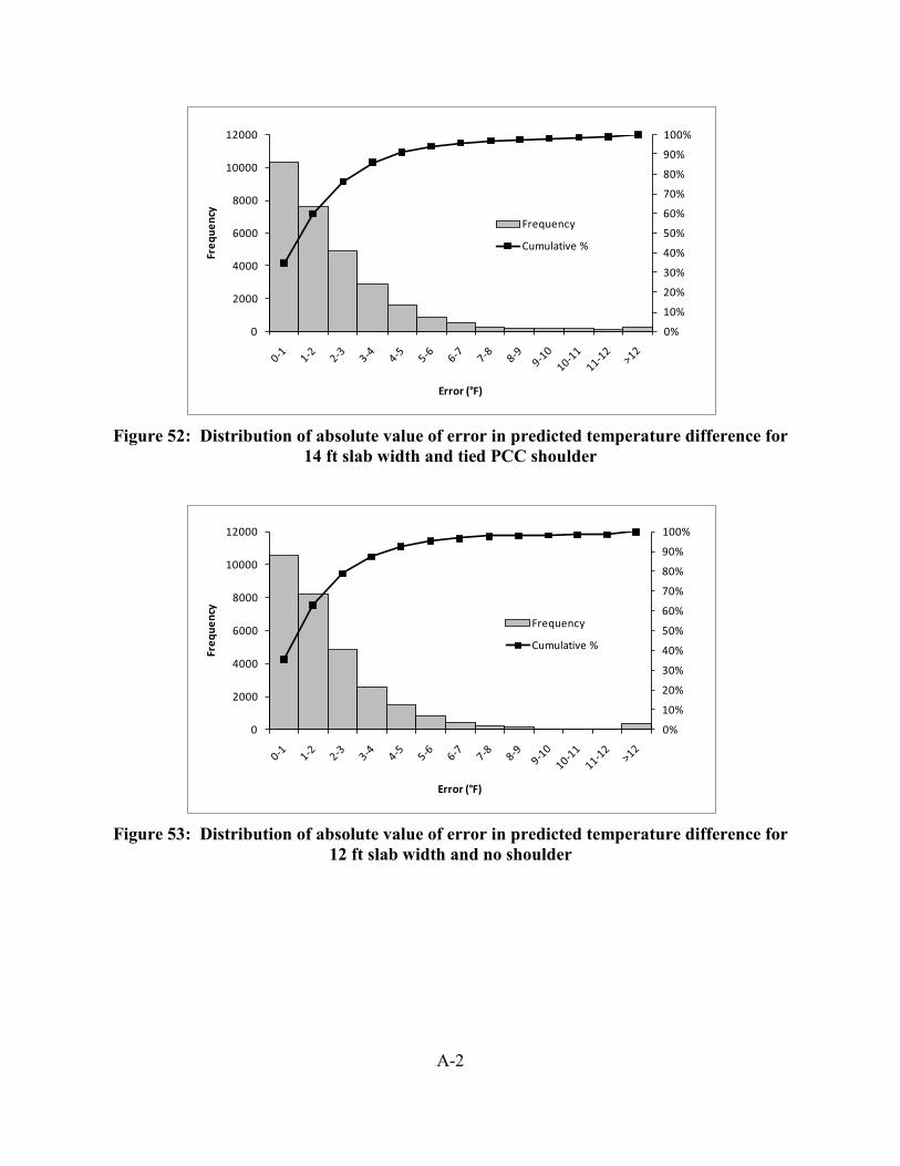
A-2
Figure 52: Distribution of absolute value of error in predicted temperature difference for
14 ft slab width and tied PCC shoulder
Figure 53: Distribution of absolute value of error in predicted temperature difference for
12 ft slab width and no shoulder
0%
10%
20%
30%
40%
50%
60%
70%
80%
90%
100%
0
2000
4000
6000
8000
10000
12000
Freq
uenc
y
Error (°F)
Frequency
Cumulative %
0%
10%
20%
30%
40%
50%
60%
70%
80%
90%
100%
0
2000
4000
6000
8000
10000
12000
Freq
uenc
y
Error (°F)
Frequency
Cumulative %

A-3
Figure 54: Distribution of absolute value of error in predicted temperature difference for
13 ft slab width and no shoulder
Figure 55: Distribution of absolute value of error in predicted temperature difference for
14 ft slab width and no shoulder
0%
10%
20%
30%
40%
50%
60%
70%
80%
90%
100%
0
2000
4000
6000
8000
10000
12000
Freq
uenc
y
Error (°F)
Frequency
Cumulative %
0%
10%
20%
30%
40%
50%
60%
70%
80%
90%
100%
0
2000
4000
6000
8000
10000
12000
Freq
uenc
y
Error (°F)
Frequency
Cumulative %
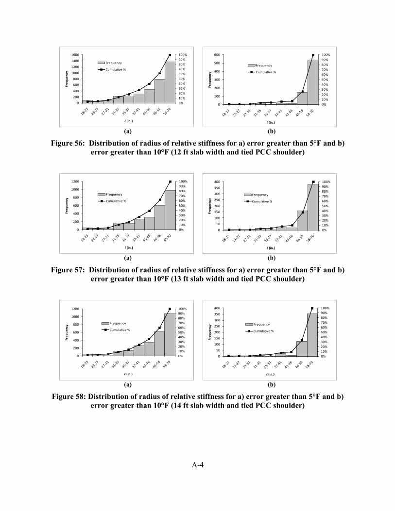
A-4
(a) (b)
Figure 56: Distribution of radius of relative stiffness for a) error greater than 5°F and b) error greater than 10°F (12 ft slab width and tied PCC shoulder)
(a) (b)
Figure 57: Distribution of radius of relative stiffness for a) error greater than 5°F and b) error greater than 10°F (13 ft slab width and tied PCC shoulder)
(a) (b)
Figure 58: Distribution of radius of relative stiffness for a) error greater than 5°F and b) error greater than 10°F (14 ft slab width and tied PCC shoulder)
0%10%20%30%40%50%60%70%80%90%100%
0
200
400
600
800
1000
1200
1400
1600
Freq
uenc
y
l (in.)
Frequency
Cumulative %
0%10%20%30%40%50%60%70%80%90%100%
0
100
200
300
400
500
600
Freq
uenc
y
l (in.)
Frequency
Cumulative %
0%10%20%30%40%50%60%70%80%90%100%
0
200
400
600
800
1000
1200
Freq
uenc
y
l (in.)
Frequency
Cumulative %
0%10%20%30%40%50%60%70%80%90%100%
0
50
100
150
200
250
300
350
400
Freq
uenc
y
l (in.)
Frequency
Cumulative %
0%10%20%30%40%50%60%70%80%90%100%
0
200
400
600
800
1000
1200
Freq
uenc
y
l (in.)
Frequency
Cumulative %
0%10%20%30%40%50%60%70%80%90%100%
0
50
100
150
200
250
300
350
400
Freq
uenc
y
l (in.)
Frequency
Cumulative %
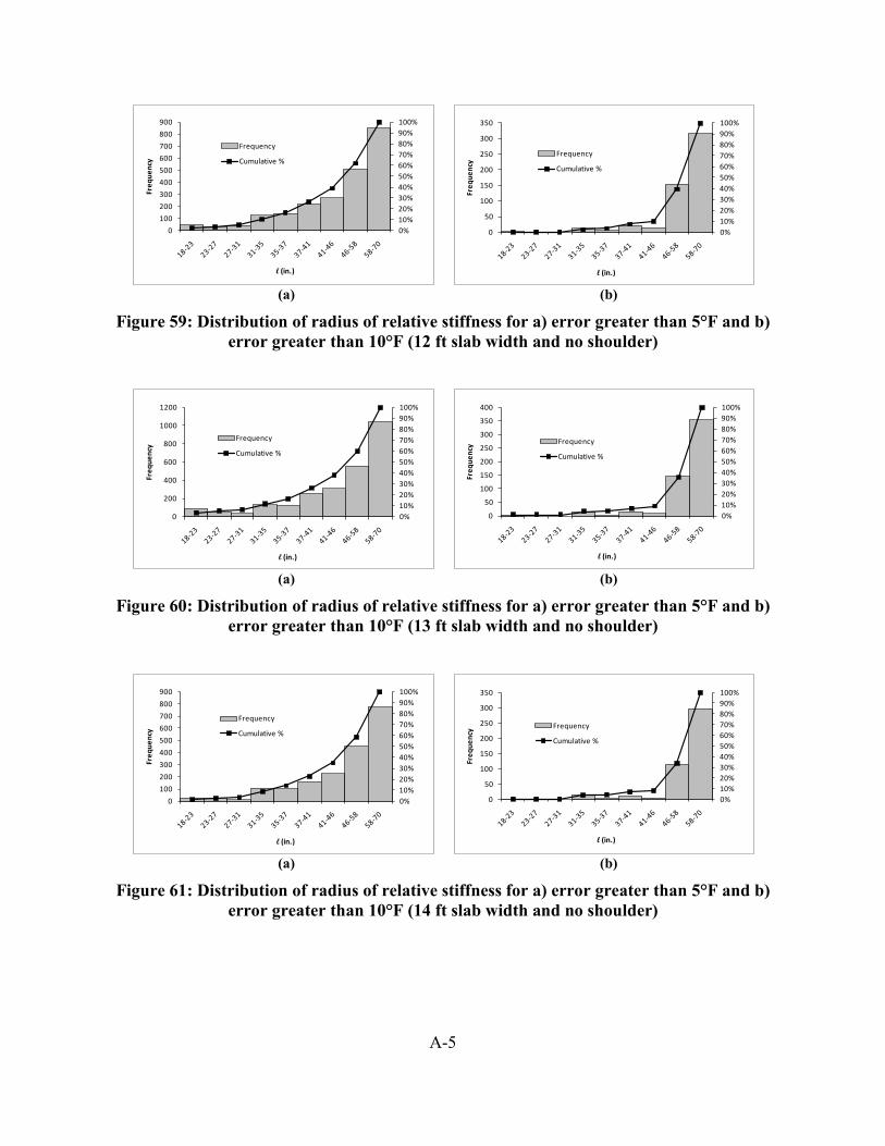
A-5
(a) (b)
Figure 59: Distribution of radius of relative stiffness for a) error greater than 5°F and b) error greater than 10°F (12 ft slab width and no shoulder)
(a) (b)
Figure 60: Distribution of radius of relative stiffness for a) error greater than 5°F and b) error greater than 10°F (13 ft slab width and no shoulder)
(a) (b)
Figure 61: Distribution of radius of relative stiffness for a) error greater than 5°F and b) error greater than 10°F (14 ft slab width and no shoulder)
0%10%20%30%40%50%60%70%80%90%100%
0
100
200
300
400
500
600
700
800
900
Freq
uenc
y
l (in.)
Frequency
Cumulative %
0%10%20%30%40%50%60%70%80%90%100%
0
50
100
150
200
250
300
350
Freq
uenc
y
l (in.)
Frequency
Cumulative %
0%10%20%30%40%50%60%70%80%90%100%
0
200
400
600
800
1000
1200
Freq
uenc
y
l (in.)
Frequency
Cumulative %
0%10%20%30%40%50%60%70%80%90%100%
0
50
100
150
200
250
300
350
400
Freq
uenc
y
l (in.)
Frequency
Cumulative %
0%10%20%30%40%50%60%70%80%90%100%
0
100
200
300
400
500
600
700
800
900
Freq
uenc
y
l (in.)
Frequency
Cumulative %
0%10%20%30%40%50%60%70%80%90%100%
0
50
100
150
200
250
300
350
Freq
uenc
y
l (in.)
Frequency
Cumulative %
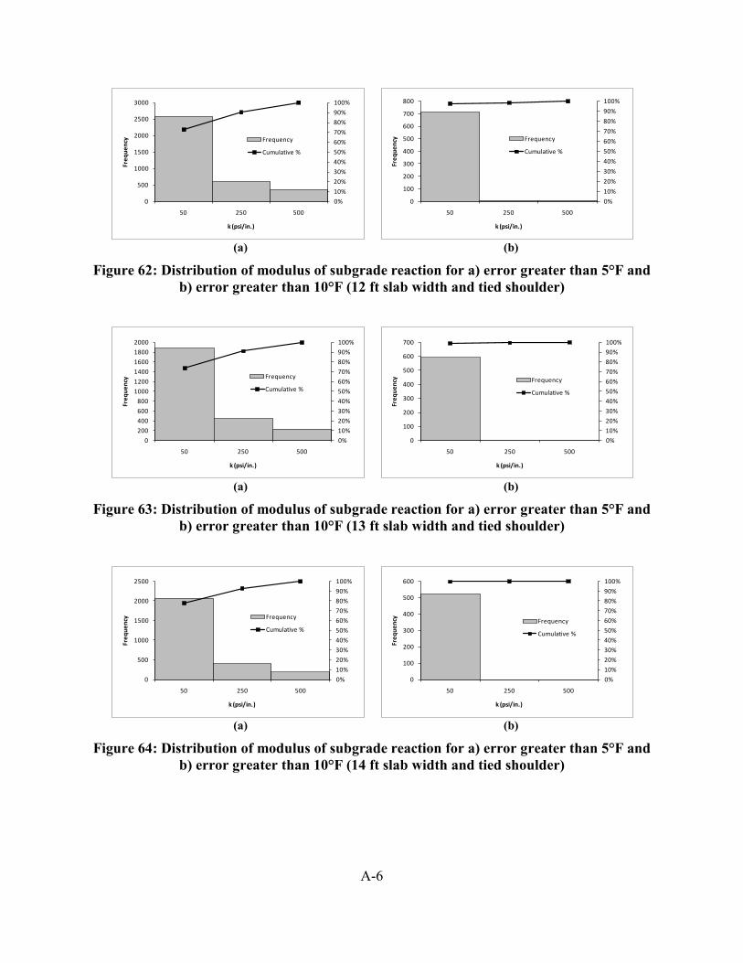
A-6
(a) (b)
Figure 62: Distribution of modulus of subgrade reaction for a) error greater than 5°F and b) error greater than 10°F (12 ft slab width and tied shoulder)
(a) (b)
Figure 63: Distribution of modulus of subgrade reaction for a) error greater than 5°F and b) error greater than 10°F (13 ft slab width and tied shoulder)
(a) (b)
Figure 64: Distribution of modulus of subgrade reaction for a) error greater than 5°F and b) error greater than 10°F (14 ft slab width and tied shoulder)
0%
10%
20%
30%
40%
50%
60%
70%
80%
90%
100%
0
500
1000
1500
2000
2500
3000
50 250 500
Freq
uenc
y
k (psi/in.)
Frequency
Cumulative %
0%
10%
20%
30%
40%
50%
60%
70%
80%
90%
100%
0
100
200
300
400
500
600
700
800
50 250 500
Freq
uenc
y
k (psi/in.)
Frequency
Cumulative %
0%
10%
20%
30%
40%
50%
60%
70%
80%
90%
100%
0
200
400
600
800
1000
1200
1400
1600
1800
2000
50 250 500
Freq
uenc
y
k (psi/in.)
Frequency
Cumulative %
0%
10%
20%
30%
40%
50%
60%
70%
80%
90%
100%
0
100
200
300
400
500
600
700
50 250 500
Freq
uenc
y
k (psi/in.)
Frequency
Cumulative %
0%
10%
20%
30%
40%
50%
60%
70%
80%
90%
100%
0
500
1000
1500
2000
2500
50 250 500
Freq
uenc
y
k (psi/in.)
Frequency
Cumulative %
0%
10%
20%
30%
40%
50%
60%
70%
80%
90%
100%
0
100
200
300
400
500
600
50 250 500
Freq
uenc
y
k (psi/in.)
Frequency
Cumulative %
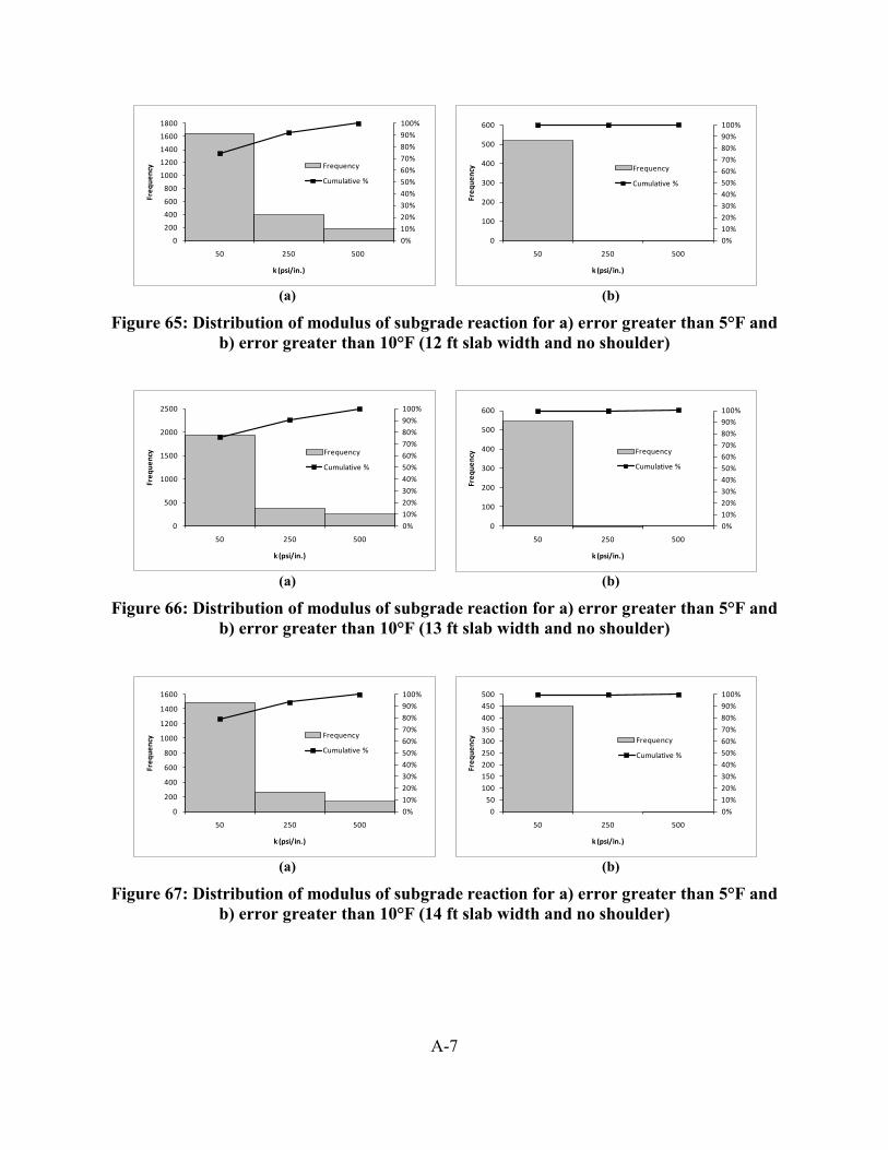
A-7
(a) (b)
Figure 65: Distribution of modulus of subgrade reaction for a) error greater than 5°F and b) error greater than 10°F (12 ft slab width and no shoulder)
(a) (b)
Figure 66: Distribution of modulus of subgrade reaction for a) error greater than 5°F and b) error greater than 10°F (13 ft slab width and no shoulder)
(a) (b)
Figure 67: Distribution of modulus of subgrade reaction for a) error greater than 5°F and b) error greater than 10°F (14 ft slab width and no shoulder)
0%
10%
20%
30%
40%
50%
60%
70%
80%
90%
100%
0
200
400
600
800
1000
1200
1400
1600
1800
50 250 500
Freq
uenc
y
k (psi/in.)
Frequency
Cumulative %
0%10%20%30%40%50%60%70%80%90%100%
0
100
200
300
400
500
600
50 250 500
Freq
uenc
y
k (psi/in.)
Frequency
Cumulative %
0%
10%
20%
30%
40%
50%
60%
70%
80%
90%
100%
0
500
1000
1500
2000
2500
50 250 500
Freq
uenc
y
k (psi/in.)
Frequency
Cumulative %
0%10%20%30%40%50%60%70%80%90%100%
0
100
200
300
400
500
600
50 250 500
Freq
uenc
y
k (psi/in.)
Frequency
Cumulative %
0%
10%
20%
30%
40%
50%
60%
70%
80%
90%
100%
0
200
400
600
800
1000
1200
1400
1600
50 250 500
Freq
uenc
y
k (psi/in.)
Frequency
Cumulative %
0%
10%
20%
30%
40%
50%
60%
70%
80%
90%
100%
0
50
100
150
200
250
300
350
400
450
500
50 250 500
Freq
uenc
y
k (psi/in.)
Frequency
Cumulative %
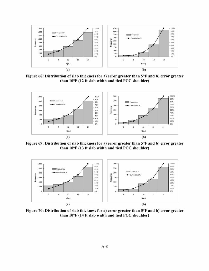
A-8
(a) (b)
Figure 68: Distribution of slab thickness for a) error greater than 5°F and b) error greater than 10°F (12 ft slab width and tied PCC shoulder)
(a) (b)
Figure 69: Distribution of slab thickness for a) error greater than 5°F and b) error greater than 10°F (13 ft slab width and tied PCC shoulder)
(a) (b)
Figure 70: Distribution of slab thickness for a) error greater than 5°F and b) error greater than 10°F (14 ft slab width and tied PCC shoulder)
0%
10%
20%
30%
40%
50%
60%
70%
80%
90%
100%
0
200
400
600
800
1000
1200
1400
1600
6 8 10 12 14
Freq
uenc
y
h (in.)
Frequency
Cumulative %
0%
10%
20%
30%
40%
50%
60%
70%
80%
90%
100%
0
50
100
150
200
250
300
350
400
450
6 8 10 12 14
Freq
uenc
y
h (in.)
Frequency
Cumulative %
0%10%20%30%40%50%60%70%80%90%100%
0
200
400
600
800
1000
1200
6 8 10 12 14
Freq
uenc
y
h (in.)
Frequency
Cumulative %
0%
10%
20%
30%
40%
50%
60%
70%
80%
90%
100%
0
50
100
150
200
250
300
6 8 10 12 14
Freq
uenc
y
h (in.)
Frequency
Cumulative %
0%10%20%30%40%50%60%70%80%90%100%
0
200
400
600
800
1000
1200
6 8 10 12 14
Freq
uenc
y
h (in.)
Frequency
Cumulative %
0%
10%
20%
30%
40%
50%
60%
70%
80%
90%
100%
0
50
100
150
200
250
300
6 8 10 12 14
Freq
uenc
y
h (in.)
Frequency
Cumulative %

A-9
(a) (b)
Figure 71: Distribution of slab thickness for a) error greater than 5°F and b) error greater than 10°F (12 ft slab width and no shoulder)
(a) (b)
Figure 72: Distribution of slab thickness for a) error greater than 5°F and b) error greater than 10°F (13 ft slab width and no shoulder)
(a) (b)
Figure 73: Distribution of slab thickness for a) error greater than 5°F and b) error greater than 10°F (14 ft slab width and no shoulder)
0%
10%
20%
30%
40%
50%
60%
70%
80%
90%
100%
0
100
200
300
400
500
600
700
800
900
1000
6 8 10 12 14
Freq
uenc
y
h (in.)
Frequency
Cumulative %
0%
10%
20%
30%
40%
50%
60%
70%
80%
90%
100%
0
50
100
150
200
250
6 8 10 12 14
Freq
uenc
y
h (in.)
Frequency
Cumulative %
0%
10%
20%
30%
40%
50%
60%
70%
80%
90%
100%
0
200
400
600
800
1000
1200
6 8 10 12 14
Freq
uenc
y
h (in.)
Frequency
Cumulative %
0%10%20%30%40%50%60%70%80%90%100%
0
50
100
150
200
250
300
6 8 10 12 14
Freq
uenc
y
h (in.)
Frequency
Cumulative %
0%10%20%30%40%50%60%70%80%90%100%
0
100
200
300
400
500
600
700
800
6 8 10 12 14
Freq
uenc
y
h (in.)
Frequency
Cumulative %
0%10%20%30%40%50%60%70%80%90%100%
0
50
100
150
200
250
6 8 10 12 14
Freq
uenc
y
h (in.)
Frequency
Cumulative %

A-10
(a) (b)
Figure 74: Distribution of temperature difference for a) error greater than 5°F and b) error greater than 10°F (12 ft slab width and tied PCC shoulder)
(a) (b)
Figure 75: Distribution of temperature difference for a) error greater than 5°F and b) error greater than 10°F (13 ft slab width and tied PCC shoulder)
(a) (b)
Figure 76: Distribution of temperature difference for a) error greater than 5°F and b) error greater than 10°F (14 ft slab width and tied PCC shoulder)
0%
10%
20%
30%
40%
50%
60%
70%
80%
90%
100%
0
200
400
600
800
1000
1200
-80 -70 -60 -50 -40 -30 -20 -10 0
Freq
uenc
y
ΔT (°F)
Frequency
Cumulative %
0%
10%
20%
30%
40%
50%
60%
70%
80%
90%
100%
0
50
100
150
200
250
300
350
400
-80 -70 -60 -50 -40 -30 -20 -10 0
Freq
uenc
y
ΔT (°F)
Frequency
Cumulative %
0%10%20%30%40%50%60%70%80%90%100%
0
200
400
600
800
1000
1200
1400
1600
-80 -70 -60 -50 -40 -30 -20 -10 0
Freq
uenc
y
ΔT (°F)
Frequency
Cumulative %
0%10%20%30%40%50%60%70%80%90%100%
0
100
200
300
400
500
600
-80 -70 -60 -50 -40 -30 -20 -10 0
Freq
uenc
y
ΔT (°F)
Frequency
Cumulative %
0%
10%
20%
30%
40%
50%
60%
70%
80%
90%
100%
0
200
400
600
800
1000
1200
1400
-80 -70 -60 -50 -40 -30 -20 -10 0
Freq
uenc
y
ΔT (°F)
Frequency
Cumulative %
0%
10%
20%
30%
40%
50%
60%
70%
80%
90%
100%
0
50
100
150
200
250
300
350
400
450
500
-80 -70 -60 -50 -40 -30 -20 -10 0
Freq
uenc
y
ΔT (°F)
Frequency
Cumulative %

A-11
(a) (b)
Figure 77: Distribution of temperature difference for a) error greater than 5°F and b) error greater than 10°F (12 ft slab width and no shoulder)
(a) (b)
Figure 78: Distribution of temperature difference for a) error greater than 5°F and b) error greater than 10°F (13 ft slab width and no shoulder)
(a) (b)
Figure 79: Distribution of temperature difference for a) error greater than 5°F and b) error greater than 10°F (14 ft slab width and no shoulder)
0%10%20%30%40%50%60%70%80%90%100%
0
200
400
600
800
1000
1200
1400
-80 -70 -60 -50 -40 -30 -20 -10 0
Freq
uenc
y
ΔT (°F)
Frequency
Cumulative %
0%
10%
20%
30%
40%
50%
60%
70%
80%
90%
100%
0
50
100
150
200
250
300
350
400
450
500
-80 -70 -60 -50 -40 -30 -20 -10 0
Freq
uenc
y
ΔT (°F)
Frequency
Cumulative %
0%
10%
20%
30%
40%
50%
60%
70%
80%
90%
100%
0
200
400
600
800
1000
1200
1400
-80 -70 -60 -50 -40 -30 -20 -10 0
Freq
uenc
y
ΔT (°F)
Frequency
Cumulative %
0%
10%
20%
30%
40%
50%
60%
70%
80%
90%
100%
0
100
200
300
400
500
600
-80 -70 -60 -50 -40 -30 -20 -10 0
Freq
uenc
y
ΔT (°F)
Frequency
Cumulative %
0%10%20%30%40%50%60%70%80%90%100%
0
200
400
600
800
1000
1200
-80 -70 -60 -50 -40 -30 -20 -10 0
Freq
uenc
y
ΔT (°F)
Frequency
Cumulative %
0%10%20%30%40%50%60%70%80%90%100%
0
50
100
150
200
250
300
350
400
450
-80 -70 -60 -50 -40 -30 -20 -10 0
Freq
uenc
y
ΔT (°F)
Frequency
Cumulative %
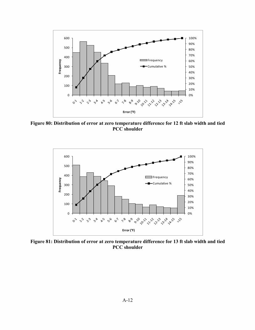
A-12
Figure 80: Distribution of error at zero temperature difference for 12 ft slab width and tied
PCC shoulder
Figure 81: Distribution of error at zero temperature difference for 13 ft slab width and tied
PCC shoulder
0%
10%
20%
30%
40%
50%
60%
70%
80%
90%
100%
0
100
200
300
400
500
600
Freq
uenc
y
Error (°F)
Frequency
Cumulative %
0%
10%
20%
30%
40%
50%
60%
70%
80%
90%
100%
0
100
200
300
400
500
600
Freq
uenc
y
Error (°F)
Frequency
Cumulative %

A-13
Figure 82: Distribution of error at zero temperature difference for 14 ft slab width and tied
PCC shoulder
Figure 83: Distribution of error at zero temperature difference for 12 ft slab width and no
shoulder
0%
10%
20%
30%
40%
50%
60%
70%
80%
90%
100%
0
50
100
150
200
250
300
350
400
450
500
Freq
uenc
y
Error (°F)
Frequency
Cumulative %
0%
10%
20%
30%
40%
50%
60%
70%
80%
90%
100%
0
100
200
300
400
500
600
Freq
uenc
y
Error (°F)
Frequency
Cumulative %

A-14
Figure 84: Distribution of error at zero temperature difference for 13 ft slab width and no
shoulder
Figure 85: Distribution of error at zero temperature difference for 14 ft slab width and no
shoulder
0%
10%
20%
30%
40%
50%
60%
70%
80%
90%
100%
0
50
100
150
200
250
300
350
400
450
500
Freq
uenc
y
Error (°F)
Frequency
Cumulative %
0%
10%
20%
30%
40%
50%
60%
70%
80%
90%
100%
0
100
200
300
400
500
600
Freq
uenc
y
Error (°F)
Frequency
Cumulative %

A-15
(a) (b)
Figure 86: Distribution of CTE for a) error greater than 5°F and b) error greater than 10°F (12 ft slab width and tied PCC shoulder)
(a) (b)
Figure 87: Distribution of CTE for a) error greater than 5°F and b) error greater than 10°F (13 ft slab width and tied PCC shoulder)
(a) (b)
Figure 88: Distribution of CTE for a) error greater than 5°F and b) error greater than 10°F (14 ft slab width and tied PCC shoulder)
0%
10%
20%
30%
40%
50%
60%
70%
80%
90%
100%
0
200
400
600
800
1000
1200
1400
1600
1800
2000
4.0 5.5 7.0
Freq
uenc
y
CTE (10-6 in./in./°F)
Frequency
Cumulative %
0%
10%
20%
30%
40%
50%
60%
70%
80%
90%
100%
0
100
200
300
400
500
600
4.0 5.5 7.0
Freq
uenc
y
CTE (10-6 in./in./°F)
Frequency
Cumulative %
0%10%20%30%40%50%60%70%80%90%100%
0
200
400
600
800
1000
1200
1400
1600
4.0 5.5 7.0
Freq
uenc
y
CTE (10-6 in./in./°F)
Frequency
Cumulative %
0%
10%
20%
30%
40%
50%
60%
70%
80%
90%
100%
0
50
100
150
200
250
300
350
4.0 5.5 7.0
Freq
uenc
y
CTE (10-6 in./in./°F)
Frequency
Cumulative %
0%
10%
20%
30%
40%
50%
60%
70%
80%
90%
100%
0
200
400
600
800
1000
1200
1400
1600
4.0 5.5 7.0
Freq
uenc
y
CTE (10-6 in./in./°F)
Frequency
Cumulative %
0%
10%
20%
30%
40%
50%
60%
70%
80%
90%
100%
0
50
100
150
200
250
300
350
4.0 5.5 7.0
Freq
uenc
y
CTE (10-6 in./in./°F)
Frequency
Cumulative %
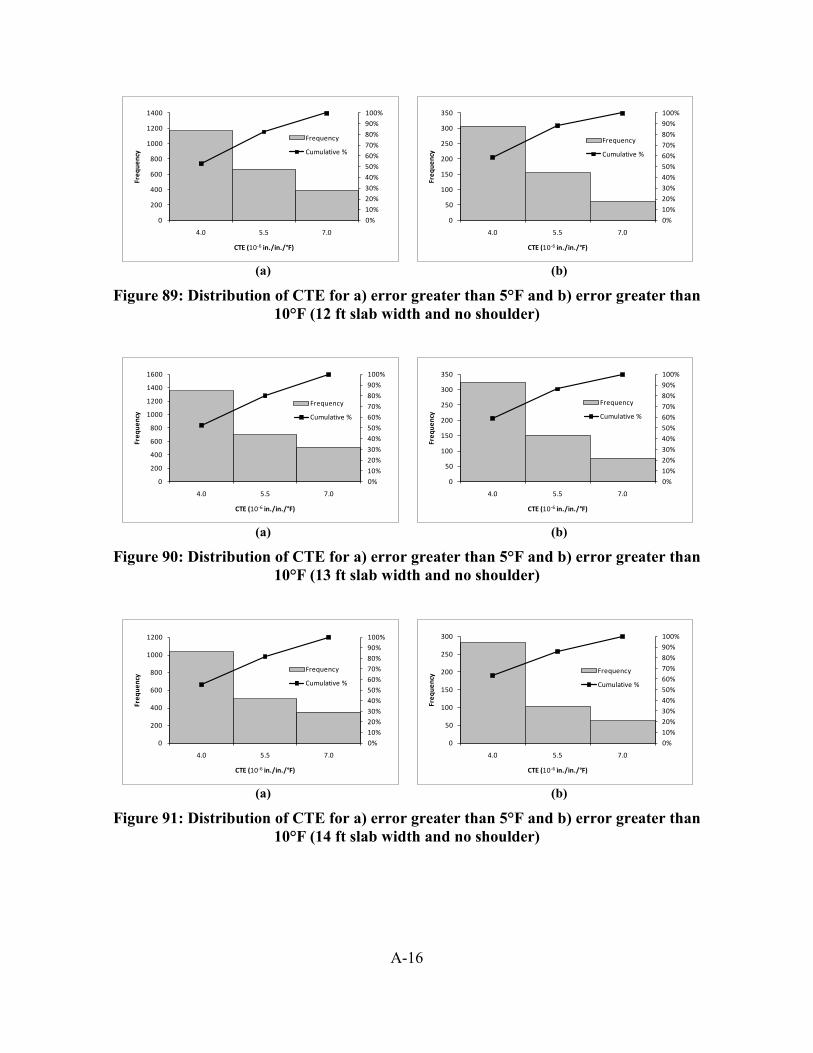
A-16
(a) (b)
Figure 89: Distribution of CTE for a) error greater than 5°F and b) error greater than 10°F (12 ft slab width and no shoulder)
(a) (b)
Figure 90: Distribution of CTE for a) error greater than 5°F and b) error greater than 10°F (13 ft slab width and no shoulder)
(a) (b)
Figure 91: Distribution of CTE for a) error greater than 5°F and b) error greater than 10°F (14 ft slab width and no shoulder)
0%
10%
20%
30%
40%
50%
60%
70%
80%
90%
100%
0
200
400
600
800
1000
1200
1400
4.0 5.5 7.0
Freq
uenc
y
CTE (10-6 in./in./°F)
Frequency
Cumulative %
0%
10%
20%
30%
40%
50%
60%
70%
80%
90%
100%
0
50
100
150
200
250
300
350
4.0 5.5 7.0
Freq
uenc
y
CTE (10-6 in./in./°F)
Frequency
Cumulative %
0%
10%
20%
30%
40%
50%
60%
70%
80%
90%
100%
0
200
400
600
800
1000
1200
1400
1600
4.0 5.5 7.0
Freq
uenc
y
CTE (10-6 in./in./°F)
Frequency
Cumulative %
0%
10%
20%
30%
40%
50%
60%
70%
80%
90%
100%
0
50
100
150
200
250
300
350
4.0 5.5 7.0
Freq
uenc
y
CTE (10-6 in./in./°F)
Frequency
Cumulative %
0%10%20%30%40%50%60%70%80%90%100%
0
200
400
600
800
1000
1200
4.0 5.5 7.0
Freq
uenc
y
CTE (10-6 in./in./°F)
Frequency
Cumulative %
0%10%20%30%40%50%60%70%80%90%100%
0
50
100
150
200
250
300
4.0 5.5 7.0
Freq
uenc
y
CTE (10-6 in./in./°F)
Frequency
Cumulative %

A-17
(a) (b)
Figure 92: Distribution of joint spacing for a) error greater than 5°F and b) error greater than 10°F (12 ft slab width and tied PCC shoulder)
(a) (b)
Figure 93: Distribution of joint spacing for a) error greater than 5°F and b) error greater than 10°F (13 ft slab width and tied PCC shoulder)
(a) (b)
Figure 94: Distribution of joint spacing for a) error greater than 5°F and b) error greater than 10°F (14 ft slab width and tied PCC shoulder)
0%10%20%30%40%50%60%70%80%90%100%
0
200
400
600
800
1000
1200
12 14 15 20
Freq
uenc
y
L (ft)
Frequency
Cumulative %
0%
10%
20%
30%
40%
50%
60%
70%
80%
90%
100%
0
50
100
150
200
250
300
350
12 14 15 20
Freq
uenc
y
L (ft)
Frequency
Cumulative %
0%10%20%30%40%50%60%70%80%90%100%
0
100
200
300
400
500
600
700
800
900
12 14 15 20
Freq
uenc
y
L (ft)
Frequency
Cumulative %
0%
10%
20%
30%
40%
50%
60%
70%
80%
90%
100%
0
50
100
150
200
250
12 14 15 20
Freq
uenc
y
L (ft)
Frequency
Cumulative %
0%
10%
20%
30%
40%
50%
60%
70%
80%
90%
100%
0
100
200
300
400
500
600
700
800
900
12 14 15 20
Freq
uenc
y
L (ft)
Frequency
Cumulative %
0%
10%
20%
30%
40%
50%
60%
70%
80%
90%
100%
0
50
100
150
200
250
12 14 15 20
Freq
uenc
y
L (ft)
Frequency
Cumulative %
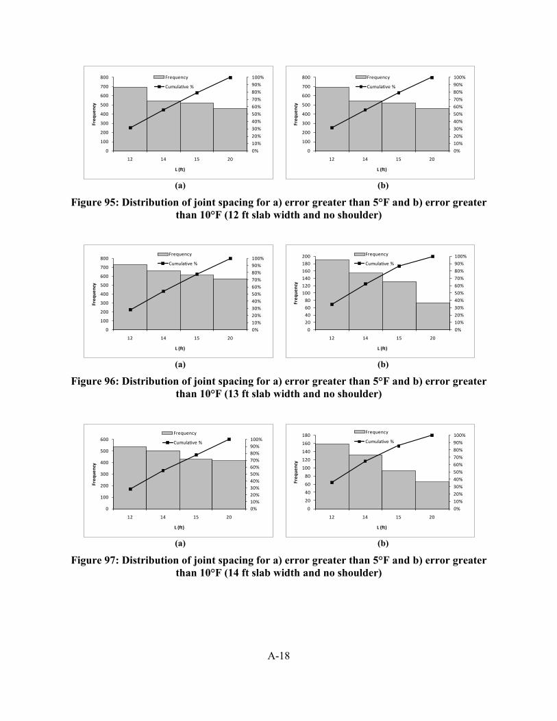
A-18
(a) (b)
Figure 95: Distribution of joint spacing for a) error greater than 5°F and b) error greater than 10°F (12 ft slab width and no shoulder)
(a) (b)
Figure 96: Distribution of joint spacing for a) error greater than 5°F and b) error greater than 10°F (13 ft slab width and no shoulder)
(a) (b)
Figure 97: Distribution of joint spacing for a) error greater than 5°F and b) error greater than 10°F (14 ft slab width and no shoulder)
0%
10%
20%
30%
40%
50%
60%
70%
80%
90%
100%
0
100
200
300
400
500
600
700
800
12 14 15 20
Freq
uenc
y
L (ft)
Frequency
Cumulative %
0%
10%
20%
30%
40%
50%
60%
70%
80%
90%
100%
0
100
200
300
400
500
600
700
800
12 14 15 20
Freq
uenc
y
L (ft)
Frequency
Cumulative %
0%10%20%30%40%50%60%70%80%90%100%
0
100
200
300
400
500
600
700
800
12 14 15 20
Freq
uenc
y
L (ft)
Frequency
Cumulative %
0%
10%
20%
30%
40%
50%
60%
70%
80%
90%
100%
0
20
40
60
80
100
120
140
160
180
200
12 14 15 20
Freq
uenc
y
L (ft)
Frequency
Cumulative %
0%10%20%30%40%50%60%70%80%90%100%
0
100
200
300
400
500
600
12 14 15 20
Freq
uenc
y
L (ft)
Frequency
Cumulative %
0%
10%
20%
30%
40%
50%
60%
70%
80%
90%
100%
0
20
40
60
80
100
120
140
160
180
12 14 15 20
Freq
uenc
y
L (ft)
Frequency
Cumulative %

A-19
(a) (b)
Figure 98: Distribution of modulus of elasticity for a) error greater than 5°F and b) error greater than 10°F (12 ft slab width and tied PCC shoulder)
(a) (b)
Figure 99: Distribution of modulus of elasticity for a) error greater than 5°F and b) error greater than 10°F (13 ft slab width and tied PCC shoulder)
(a) (b)
Figure 100: Distribution of modulus of elasticity for a) error greater than 5°F and b) error greater than 10°F (14 ft slab width and tied PCC shoulder)
0%10%20%30%40%50%60%70%80%90%100%
0
200
400
600
800
1000
1200
1400
3000000 4000000 5000000
Freq
uenc
y
E (psi)
Frequency
Cumulative %
0%10%20%30%40%50%60%70%80%90%100%
0
50
100
150
200
250
300
3000000 4000000 5000000
Freq
uenc
y
E (psi)
Frequency
Cumulative %
0%10%20%30%40%50%60%70%80%90%100%
0
200
400
600
800
1000
1200
3000000 4000000 5000000
Freq
uenc
y
E (psi)
Frequency
Cumulative %
0%10%20%30%40%50%60%70%80%90%100%
0
50
100
150
200
250
3000000 4000000 5000000
Freq
uenc
y
E (psi)
Frequency
Cumulative %
0%
10%
20%
30%
40%
50%
60%
70%
80%
90%
100%
0
200
400
600
800
1000
1200
3000000 4000000 5000000
Freq
uenc
y
E (psi)
Frequency
Cumulative %
0%
10%
20%
30%
40%
50%
60%
70%
80%
90%
100%
0
50
100
150
200
250
3000000 4000000 5000000
Freq
uenc
y
E (psi)
Frequency
Cumulative %

A-20
(a) (b)
Figure 101: Distribution of modulus of elasticity for a) error greater than 5°F and b) error greater than 10°F (12 ft slab width and no shoulder)
(a) (b)
Figure 102: Distribution of modulus of elasticity for a) error greater than 5°F and b) error greater than 10°F (13 ft slab width and no shoulder)
(a) (b)
Figure 103: Distribution of modulus of elasticity for a) error greater than 5°F and b) error greater than 10°F (14 ft slab width and no shoulder)
0%10%20%30%40%50%60%70%80%90%100%
0
100
200
300
400
500
600
700
800
900
3000000 4000000 5000000
Freq
uenc
y
E (psi)
Frequency
Cumulative %
0%10%20%30%40%50%60%70%80%90%100%
0
50
100
150
200
250
3000000 4000000 5000000
Freq
uenc
y
E (psi)
Frequency
Cumulative %
0%10%20%30%40%50%60%70%80%90%100%
0100200300400500600700800900
1000
3000000 4000000 5000000
Freq
uenc
y
E (psi)
Frequency
Cumulative %
0%
10%
20%
30%
40%
50%
60%
70%
80%
90%
100%
0
50
100
150
200
250
3000000 4000000 5000000
Freq
uenc
y
E (psi)
Frequency
Cumulative %
0%10%20%30%40%50%60%70%80%90%100%
0
100
200
300
400
500
600
700
800
3000000 4000000 5000000
Freq
uenc
y
E (psi)
Frequency
Cumulative %
0%
10%
20%
30%
40%
50%
60%
70%
80%
90%
100%
0
20
40
60
80
100
120
140
160
180
3000000 4000000 5000000
Freq
uenc
y
E (psi)
Frequency
Cumulative %
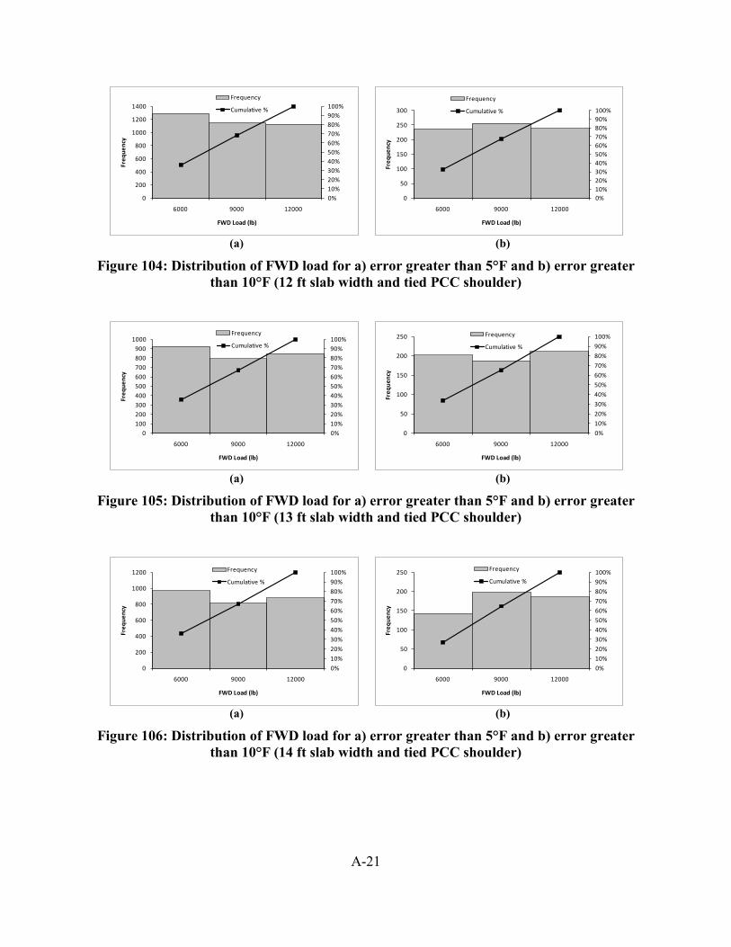
A-21
(a) (b)
Figure 104: Distribution of FWD load for a) error greater than 5°F and b) error greater than 10°F (12 ft slab width and tied PCC shoulder)
(a) (b)
Figure 105: Distribution of FWD load for a) error greater than 5°F and b) error greater than 10°F (13 ft slab width and tied PCC shoulder)
(a) (b)
Figure 106: Distribution of FWD load for a) error greater than 5°F and b) error greater than 10°F (14 ft slab width and tied PCC shoulder)
0%10%20%30%40%50%60%70%80%90%100%
0
200
400
600
800
1000
1200
1400
6000 9000 12000
Freq
uenc
y
FWD Load (lb)
Frequency
Cumulative %
0%10%20%30%40%50%60%70%80%90%100%
0
50
100
150
200
250
300
6000 9000 12000
Freq
uenc
y
FWD Load (lb)
Frequency
Cumulative %
0%10%20%30%40%50%60%70%80%90%100%
0100200300400500600700800900
1000
6000 9000 12000
Freq
uenc
y
FWD Load (lb)
Frequency
Cumulative %
0%
10%
20%
30%
40%
50%
60%
70%
80%
90%
100%
0
50
100
150
200
250
6000 9000 12000
Freq
uenc
y
FWD Load (lb)
Frequency
Cumulative %
0%10%20%30%40%50%60%70%80%90%100%
0
200
400
600
800
1000
1200
6000 9000 12000
Freq
uenc
y
FWD Load (lb)
Frequency
Cumulative %
0%10%20%30%40%50%60%70%80%90%100%
0
50
100
150
200
250
6000 9000 12000
Freq
uenc
y
FWD Load (lb)
Frequency
Cumulative %

A-22
(a) (b)
Figure 107: Distribution of FWD load for a) error greater than 5°F and b) error greater than 10°F (12 ft slab width and no shoulder)
(a) (b)
Figure 108: Distribution of FWD load for a) error greater than 5°F and b) error greater than 10°F (13 ft slab width and no shoulder)
(a) (b)
Figure 109: Distribution of FWD load for a) error greater than 5°F and b) error greater than 10°F (14 ft slab width and no shoulder)
0%
10%
20%
30%
40%
50%
60%
70%
80%
90%
100%
0
100
200
300
400
500
600
700
800
900
1000
6000 9000 12000
Freq
uenc
y
FWD Load (lb)
Frequency
Cumulative %
0%10%20%30%40%50%60%70%80%90%100%
020406080
100120140160180200
6000 9000 12000
Freq
uenc
y
FWD Load (lb)
Frequency
Cumulative %
0%10%20%30%40%50%60%70%80%90%100%
0100200300400500600700800900
1000
6000 9000 12000
Freq
uenc
y
FWD Load (lb)
Frequency
Cumulative %
0%10%20%30%40%50%60%70%80%90%100%
020406080
100120140160180200
6000 9000 12000
Freq
uenc
y
FWD Load (lb)
Frequency
Cumulative %
0%10%20%30%40%50%60%70%80%90%100%
0
100
200
300
400
500
600
700
800
6000 9000 12000
Freq
uenc
y
FWD Load (lb)
Frequency
Cumulative %
0%10%20%30%40%50%60%70%80%90%100%
0
20
40
60
80
100
120
140
160
180
6000 9000 12000
Freq
uenc
y
FWD Load (lb)
Frequency
Cumulative %
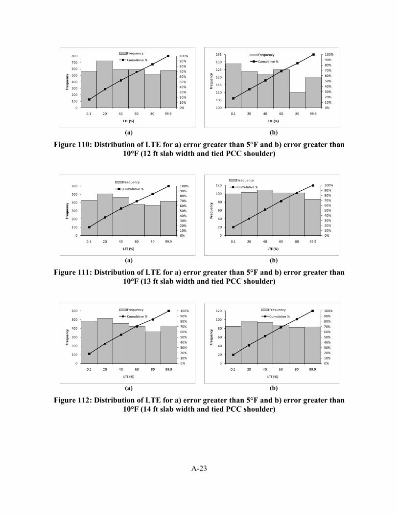
A-23
(a) (b)
Figure 110: Distribution of LTE for a) error greater than 5°F and b) error greater than 10°F (12 ft slab width and tied PCC shoulder)
(a) (b)
Figure 111: Distribution of LTE for a) error greater than 5°F and b) error greater than 10°F (13 ft slab width and tied PCC shoulder)
(a) (b)
Figure 112: Distribution of LTE for a) error greater than 5°F and b) error greater than 10°F (14 ft slab width and tied PCC shoulder)
0%10%20%30%40%50%60%70%80%90%100%
0
100
200
300
400
500
600
700
800
0.1 20 40 60 80 99.9
Freq
uenc
y
LTE (%)
Frequency
Cumulative %
0%
10%
20%
30%
40%
50%
60%
70%
80%
90%
100%
100
105
110
115
120
125
130
135
0.1 20 40 60 80 99.9
Freq
uenc
y
LTE (%)
Frequency
Cumulative %
0%10%20%30%40%50%60%70%80%90%100%
0
100
200
300
400
500
600
0.1 20 40 60 80 99.9
Freq
uenc
y
LTE (%)
Frequency
Cumulative %
0%10%20%30%40%50%60%70%80%90%100%
0
20
40
60
80
100
120
0.1 20 40 60 80 99.9
Freq
uenc
y
LTE (%)
Frequency
Cumulative %
0%
10%
20%
30%
40%
50%
60%
70%
80%
90%
100%
0
100
200
300
400
500
600
0.1 20 40 60 80 99.9
Freq
uenc
y
LTE (%)
Frequency
Cumulative %
0%
10%
20%
30%
40%
50%
60%
70%
80%
90%
100%
0
20
40
60
80
100
120
0.1 20 40 60 80 99.9
Freq
uenc
y
LTE (%)
Frequency
Cumulative %
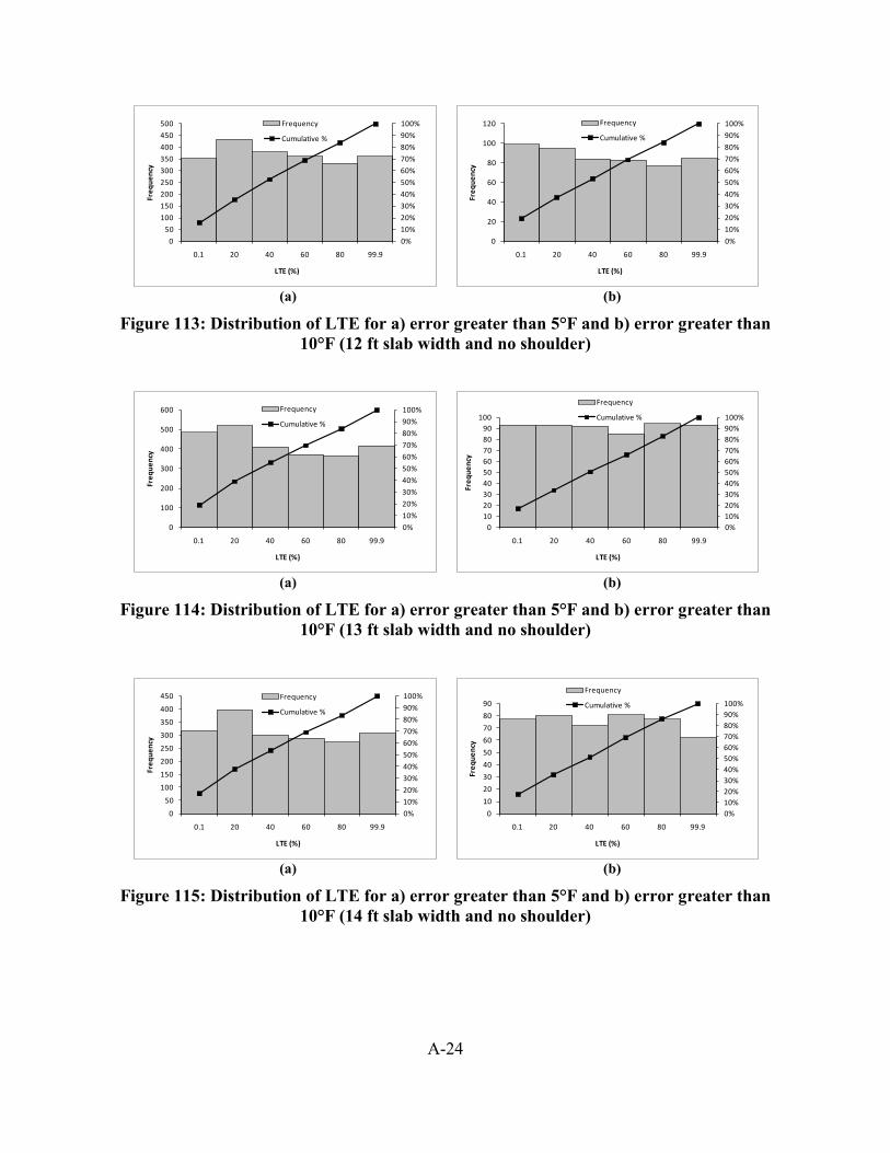
A-24
(a) (b)
Figure 113: Distribution of LTE for a) error greater than 5°F and b) error greater than 10°F (12 ft slab width and no shoulder)
(a) (b)
Figure 114: Distribution of LTE for a) error greater than 5°F and b) error greater than 10°F (13 ft slab width and no shoulder)
(a) (b)
Figure 115: Distribution of LTE for a) error greater than 5°F and b) error greater than 10°F (14 ft slab width and no shoulder)
0%
10%
20%
30%
40%
50%
60%
70%
80%
90%
100%
0
50
100
150
200
250
300
350
400
450
500
0.1 20 40 60 80 99.9
Freq
uenc
y
LTE (%)
Frequency
Cumulative %
0%
10%
20%
30%
40%
50%
60%
70%
80%
90%
100%
0
20
40
60
80
100
120
0.1 20 40 60 80 99.9
Freq
uenc
y
LTE (%)
Frequency
Cumulative %
0%
10%
20%
30%
40%
50%
60%
70%
80%
90%
100%
0
100
200
300
400
500
600
0.1 20 40 60 80 99.9
Freq
uenc
y
LTE (%)
Frequency
Cumulative %
0%10%20%30%40%50%60%70%80%90%100%
0102030405060708090
100
0.1 20 40 60 80 99.9
Freq
uenc
y
LTE (%)
Frequency
Cumulative %
0%
10%
20%
30%
40%
50%
60%
70%
80%
90%
100%
0
50
100
150
200
250
300
350
400
450
0.1 20 40 60 80 99.9
Freq
uenc
y
LTE (%)
Frequency
Cumulative %
0%10%20%30%40%50%60%70%80%90%100%
0
10
20
30
40
50
60
70
80
90
0.1 20 40 60 80 99.9
Freq
uenc
y
LTE (%)
Frequency
Cumulative %

APPENDIX B: ALPS2 PROFILER TEST PATTERN MAPS

B-1
Note: these testing pattern maps were created by Mn/DOT.
Figure 116: Cell 7 panel 12 testing configuration - June tests
-12-11-10-9-8-7-6-5-4-3-2-10123456789
1011121314
9 1087654
113875113895
P12
Passing
15
14"26"196" 178" 144" 86" 62" 44"220"
14
6"
118207.8118222.7
Indicatesdirection of ALPS2
2"
24" to joint
Use 1" laser scan spacing
Actual scan coordinates -field marks are 8" away110"238"262"
30 2
250"
15
14 & 0
1 11 12 13
20'
13'
C4
C2
C3
MP
E
JA1JB1
C1
IndicatesFWD Test Point
6"
2"
-14-13
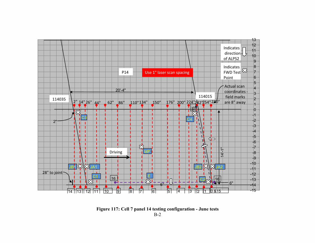
B-2
Figure 117: Cell 7 panel 14 testing configuration - June tests
-15-14-13-12-11-10-9-8-7-6-5-4-3-2-10123456789
10111213
4 3578910
114015114035
P14
Driving
16
254"242"62" 86" 134" 176" 200" 224"44"
15
6"
Indicatesdirection of ALPS2
270"
28" to joint
Use 1" laser scan spacing
Actual scan coordinates -field marks are 8" away150"26"2"
1114 12
14"
16
13 2 1 0 &15
20'-4"
14'-1
"
C2
C4C3
MP
E
JA1JB1
C1
IndicatesFWD Test Point
6"
2"
110"
6
JA2JB2

B-3
Figure 118: Cell 12 panel 19 testing configuration - June tests
& 013 14
180" Actual scan coordinates -204"192" 168"156" 138" 115" 80" 56" 38"26"14" 2" 13
field marks are 8" away126"14 11C1 C2 14
6" E 10JB1 JA1 IndicatesJB2 JA2 24" to joint 9
direction Passing 8
of ALPS2 7
1"-
Indicates 6
12'
MP FWD Test 5
Point 432
C3 C4118150 118134.6 10
-1-213 Use 1" laser scan spacing -3
0 1 2 123 4 6 75 8 9 10 11 -4-5
15'-3" -6-7-8
P19 -9-10-11-12-13-14

B-4
Figure 119: Cell 12 panel 24 testing configuration - June tests
-14-13-12-11-10-9-8-7-6-5-4-3-2-10123456789
1011121314
10 117 965321
118209.8118224.7
P24
Passing
14"26"168"156" 138" 114" 80" 38"180"
156"
118207.8118222.7
Indicatesdirection of ALPS2
12
2"
24" to joint
Use 1" laser scan spacing
Actual scan coordinates -field marks are 8" away
56"90"
15
200"192"
840 13
14 & 0
14
6"
IndicatesFWD Test Point
14'-11"
12'-1
"
C4
C2
C3
MP
EJA1JB1
C1
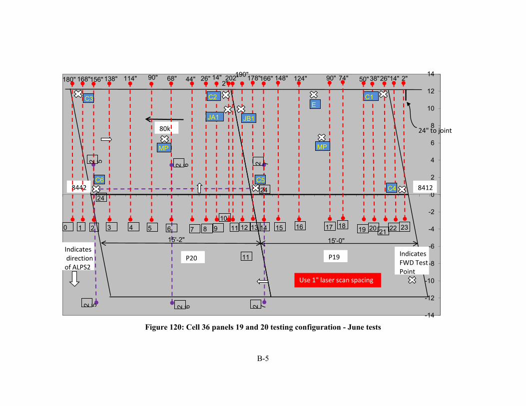
B-5
Figure 120: Cell 36 panels 19 and 20 testing configuration - June tests
-14
-12
-10
-8
-6
-4
-2
0
2
4
6
8
10
12
14
2321
84128442
P20 P19
80k 24" to joint
2"26"14"
20
38"
16
50"90"
151413
124"148"166"178"190"2"
14"26"44"68"90"114"138"156"
24
8763210 1110
9
24
11
12
2 5 2 72 6
2 72 6
Indicatesdirection of ALPS2
IndicatesFWD Test Point
Use 1" laser scan spacing
C4
C2C3
MP
E
JA1 JB1
C1
MP
C6 C5
15'-2" 15'-0"
17 18 19 22
74"202"
4 5
180" 168"
2 5

B-6
Figure 121: Cell 37 panels 8 and 9 testing configuration - June tests
-14
-12
-10
-8
-6
-4
-2
0
2
4
6
8
10
12
14
1918
87458769
P9 P8
80k24" to joint
2"26" 14"
17
38"
16
54"72"
151413
96"124"142"154"166"2"
14"26"46"72"100"118"130"142"
20 20
6543210 98
7 121110
2121 2322
2322
Indicatesdirection of ALPS2
IndicatesFWD Test Point
Use 1" laser scan spacing
C4
C2C3
MP
E
JA1 JB1
C1
MP
C6
C5
12'-0" 12'-1"

B-7
Figure 122: Cell 53 panel 3 testing configuration - June tests
-14-13-12-11-10-9-8-7-6-5-4-3-2-10123456789
1011121314
1
12
03 245678
2114521160
P4
15
15'-0"
12" to joint911 10
12
1414
6"
Indicatesdirection of ALPS2
IndicatesFWD Test Point
JA1JB1 C
1C2
C4
C3
E
MP
14"26"166" 144"126" 78"62" 38"190" 102" 50"178" Actual scan coordinates -field marks are 8" away
Driving
15
1313
Use 1" laser scan spacing

B-8
Figure 123: Cell 205 panel 18 testing configuration - June tests
-14-13-12-11-10-9-8-7-6-5-4-3-2-10123456789
1011121314
8 106 753210
112850112865
P18
Passing
11
14"26"168"150" 126" 90" 68" 44"176" 2"
6"
Indicatesdirection of ALPS2
Use 1" laser scan spacing
Actual scan coordinates -field marks are 8" away
9
112"
4
14'-10.5"
12'-1
1"
116"
C1
C4C3
MP
C2E
JA1JB1
IndicatesFWD Test Point
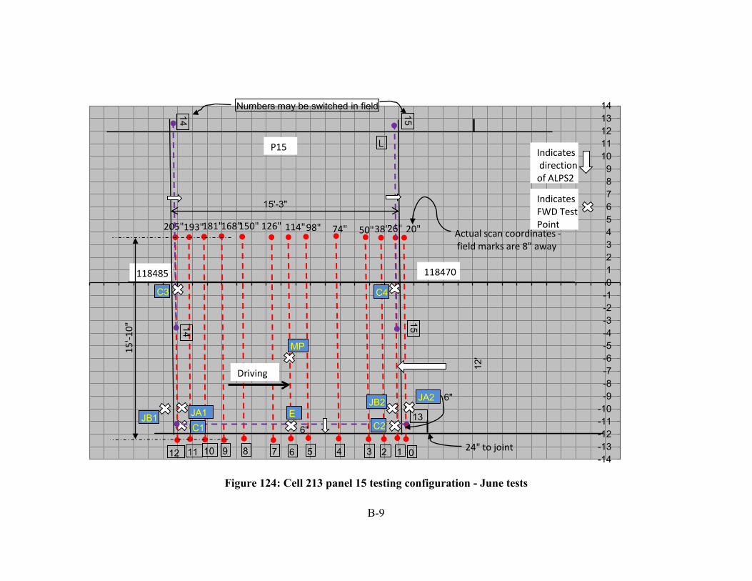
B-9
Figure 124: Cell 213 panel 15 testing configuration - June tests
-14-13-12-11-10-9-8-7-6-5-4-3-2-10123456789
1011121314
1
14
03 245678
118470118485
P15
13
L
15'-3"
12'
24" to joint91112 10
14
1515
Numbers may be switched in field
6"
6"
Indicatesdirection of ALPS2
IndicatesFWD Test Point
JA1JB1C1 C2
C4C3
E
MP
26"38"181"168"150" 114"98" 50"205" 20"126" 74"193"Actual scan coordinates -field marks are 8" away
JA2JB2
Driving
15'-1
0"
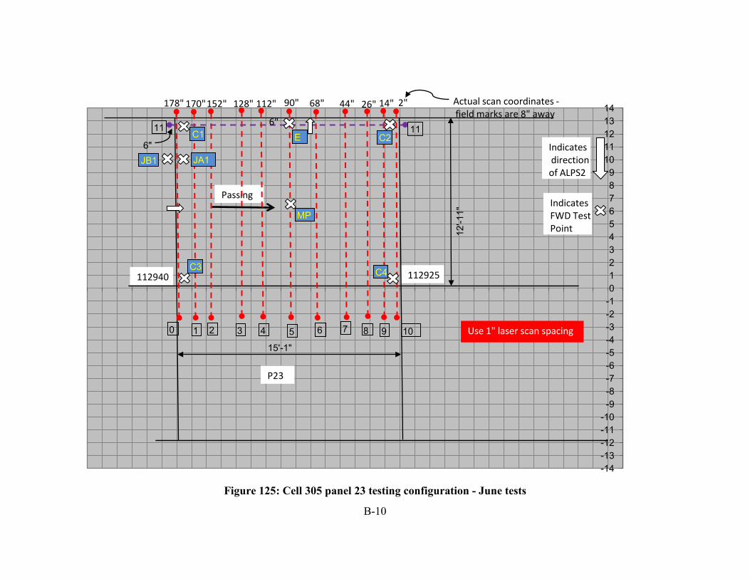
B-10
Figure 125: Cell 305 panel 23 testing configuration - June tests
-14-13-12-11-10-9-8-7-6-5-4-3-2-10123456789
1011121314
8 106 753210
112925112940
P23
Passing
11
14"26"170"152" 128" 90" 68" 44"178" 2"
6"
Indicatesdirection of ALPS2
Use 1" laser scan spacing
Actual scan coordinates -field marks are 8" away
9
112"
4
15'-1"
12'-1
1"
6"
11
IndicatesFWD Test Point
C1
C4C3
MP
C2E
JA1JB1
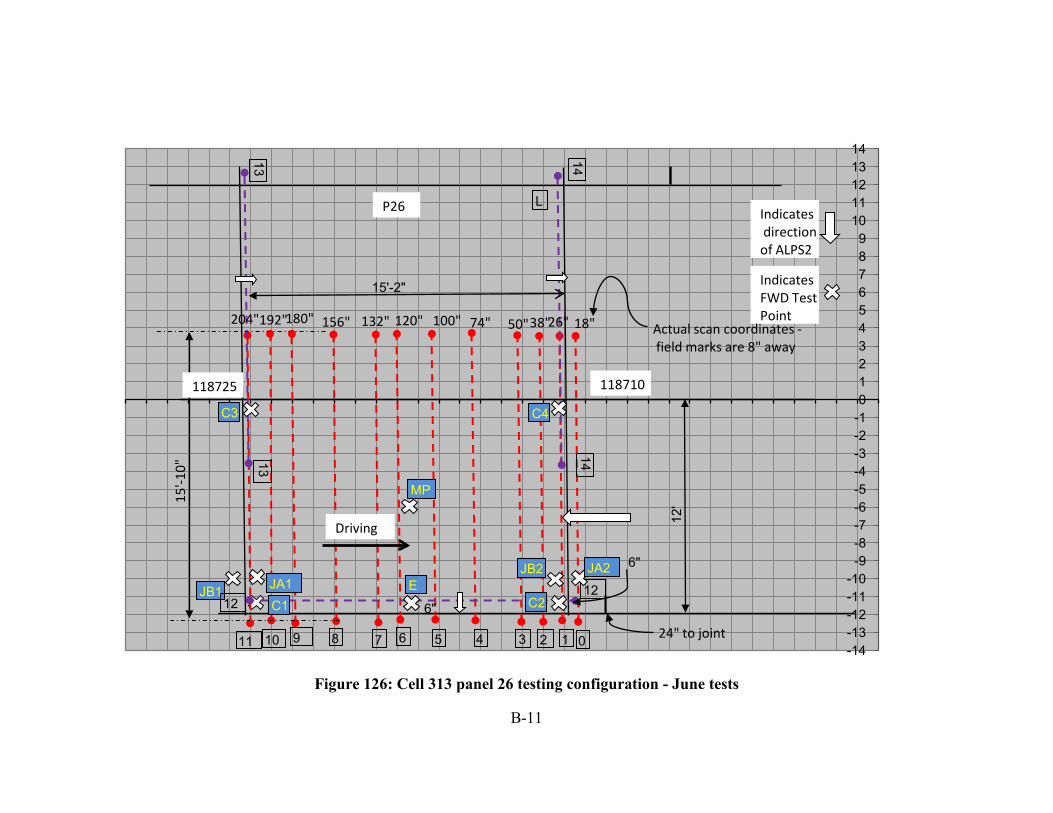
B-11
Figure 126: Cell 313 panel 26 testing configuration - June tests
-14-13-12-11-10-9-8-7-6-5-4-3-2-10123456789
1011121314
1
13
03 245678
118710
P26
12
L
15'-2"
12'
24" to joint1011 9
13
1414
6"
6"
Indicatesdirection of ALPS2
IndicatesFWD Test Point
JA1JB1C1 C2
C4C3
E
MP
26"38"180" 156" 120" 100" 50"204" 18"132" 74"192"
12
Actual scan coordinates -field marks are 8" away
JA2JB2
Driving
15'-1
0"
118725

B-12
Figure 127: cell 513 panel 5 testing configuration - June tests
-14-13-12-11-10-9-8-7-6-5-4-3-2-10123456789
1011121314
1
11
03 245678
118410118422
P5
10
12'
12'
24" to joint9
11
1212
6"
6"
Indicatesdirection of ALPS2
IndicatesFWD Test Point
JA1JB1
C1 C2
C4C3
E
MP
26"42"166"154" 118" 96" 56" 14"142" 72"
10
Actual scan coordinates -field marks are 8" away
JA2JB2
Driving
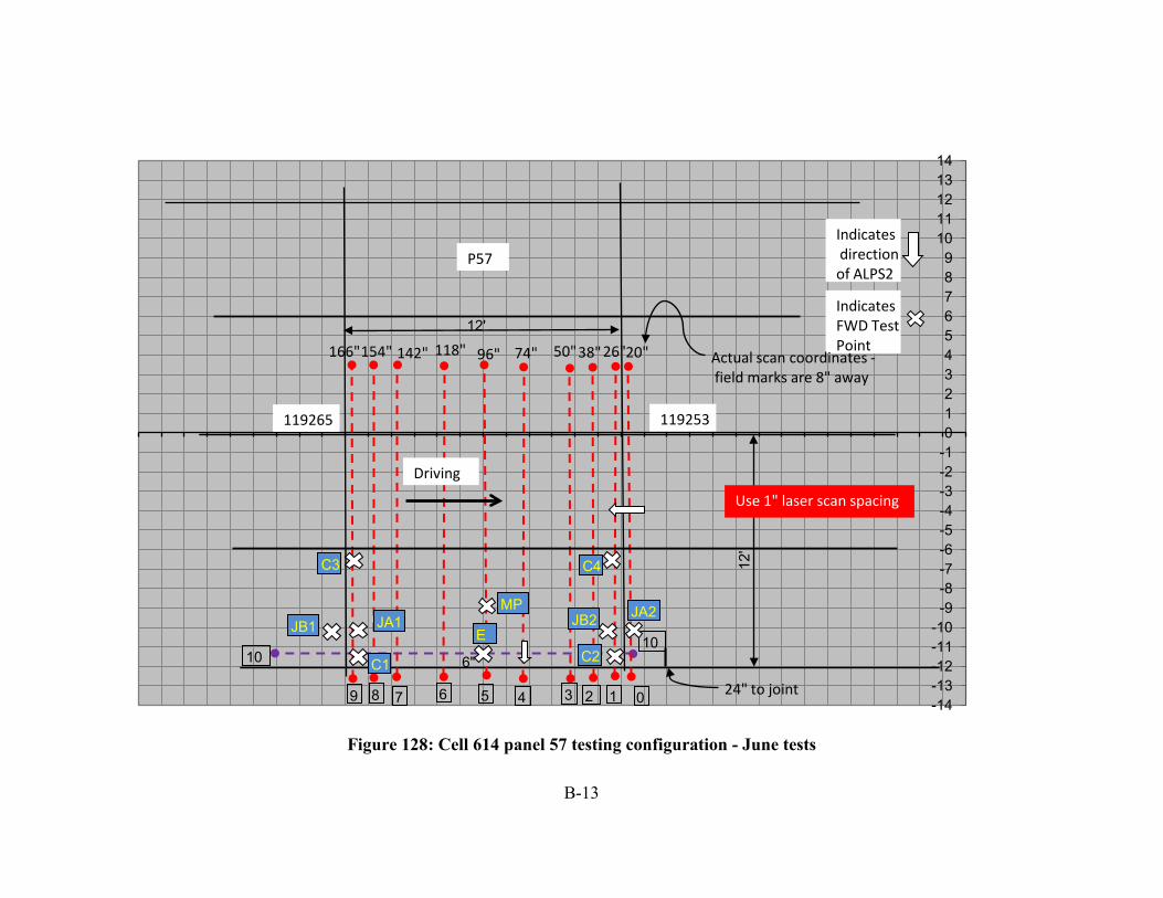
B-13
Figure 128: Cell 614 panel 57 testing configuration - June tests
-14-13-12-11-10-9-8-7-6-5-4-3-2-10123456789
1011121314
1 03 245678
119253119265
P57
10
12'
12'
24" to joint9
6"
Indicatesdirection of ALPS2
IndicatesFWD Test Point
JA1JB1
C1 C2
C4C3
E
MP
26"38"166"154" 118" 96" 50" 20"142" 74"
10
Actual scan coordinates -field marks are 8" away
JA2JB2
Driving
Use 1" laser scan spacing

B-14
Figure 129: Cell 7 panel 14 testing configuration – October tests
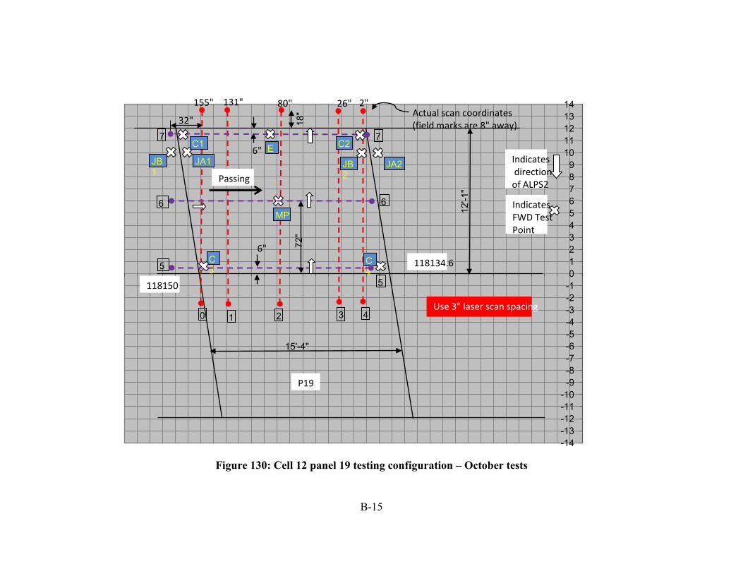
B-15
Figure 130: Cell 12 panel 19 testing configuration – October tests
-14-13-12-11-10-9-8-7-6-5-4-3-2-10123456789
1011121314
3 4
6
20
118134.6
118150
P19
Passing
2"131" 80"155"
7
Indicatesdirection of ALPS2
6
Use 3" laser scan spacing
Actual scan coordinates (field marks are 8" away)
26"
7
1
5
IndicatesFWD Test Point
15'-4"
12'-1
"
C4
C2
C3
MP
EJA1JB
1
C1
JA2JB2
5
32"
6"
6" 72"
18"
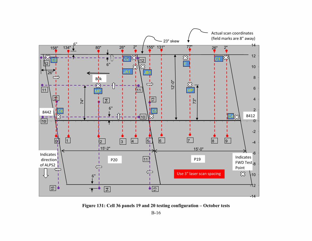
B-16
Figure 131: Cell 36 panels 19 and 20 testing configuration – October tests
-14
-12
-10
-8
-6
-4
-2
0
2
4
6
8
10
12
14
84128442
P20 P19
80k
2"
9
26"77"
65
131"155"2"26"80"134"158"
10
3210
11 11
4
10
11
15 1314
1314
Indicatesdirection of ALPS2
IndicatesFWD Test Point
Use 3" laser scan spacing
C4
C2C3
MP
E
JA1 JB1
C1
MP
C6 C5
15'-2" 15'-0"
7 8
121215
Actual scan coordinates (field marks are 8" away)
74"
26"
6"
6"
73"
6"
6"
23" skew
12'-0
"
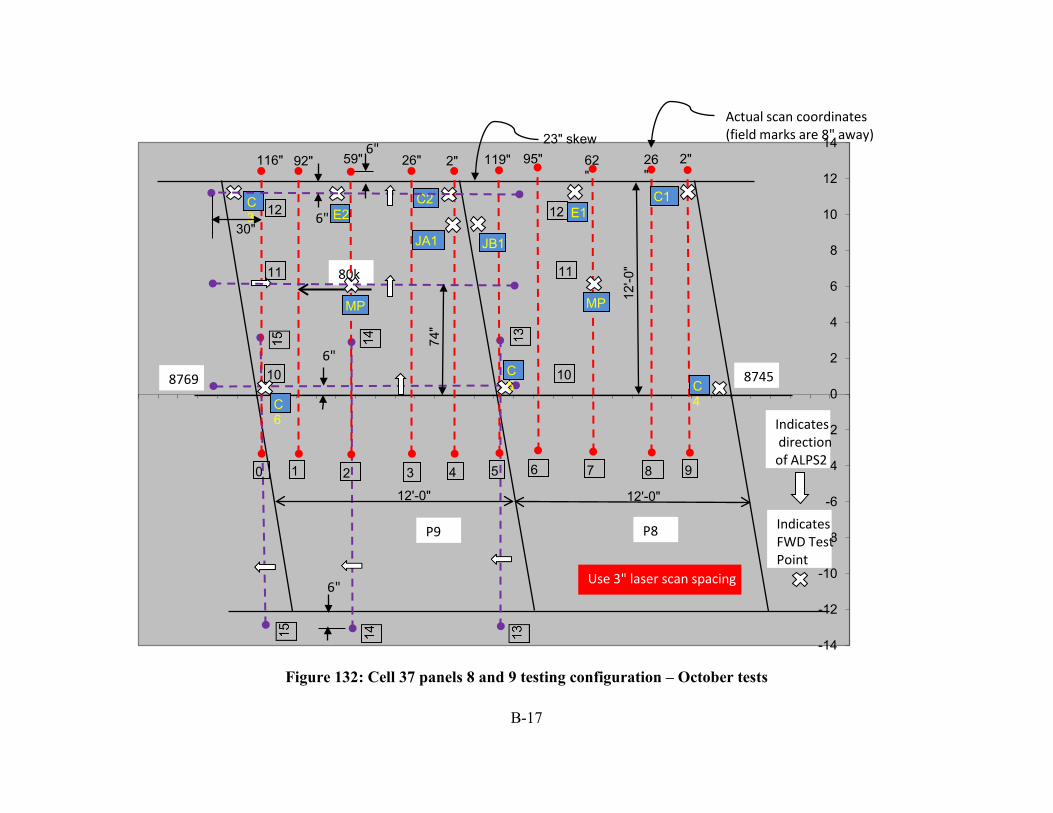
B-17
Figure 132: Cell 37 panels 8 and 9 testing configuration – October tests
-14
-12
-10
-8
-6
-4
-2
0
2
4
6
8
10
12
14
87458769
P9 P8
80k
2"
9
26"
62"
87
95"119"2"26"59"92"116"
10 10
3210 4 65
Indicatesdirection of ALPS2
IndicatesFWD Test Point
Use 3" laser scan spacing
C4
C2C3
MP
E1
JA1 JB1
C1
MP
C6
C5
12'-0" 12'-0"
E2 1212
1111
Actual scan coordinates (field marks are 8" away)
6"
6"
6"
30"
74"
6"23" skew
12'-0
"

B-18
-14-13-12-11-10-9-8-7-6-5-4-3-2-10123456789
1011121314
8
012
2114521160
P3
7
15'-1"
34
8
1010
Indicatesdirection of ALPS2
IndicatesFWD Test Point
JA1JB1C1
C2
C4
C3
E
MP
2"152" 26"86"176" Actual scan coordinates (field marks are 8" away)
Driving
7
99 Use 3" laser scan spacing
-1"
66
55
6"
72" 6"
6"
2"85"174"
Figure 133: Cell 53 panel 3 testing configuration – October tests

B-19
Figure 134: Cell 71 panel 11 testing configuration – October tests
-14-13-12-11-10-9-8-7-6-5-4-3-2-10123456789
1011121314
1 0234
P11
Driving
5
155"
2"26"
92"
179"
Indicatesdirection of ALPS2
Use 3" laser scan spacing
Actual scan coordinates shown (field marks are 8" away)
5
15'-1"
12'
C2
C1E
C3
C4
MP
JB2JA2
JB1JA1
IndicatesFWD Test Point
7 7
6 6
6" to "0" line
6"
6"72"
??????? ??????18
"
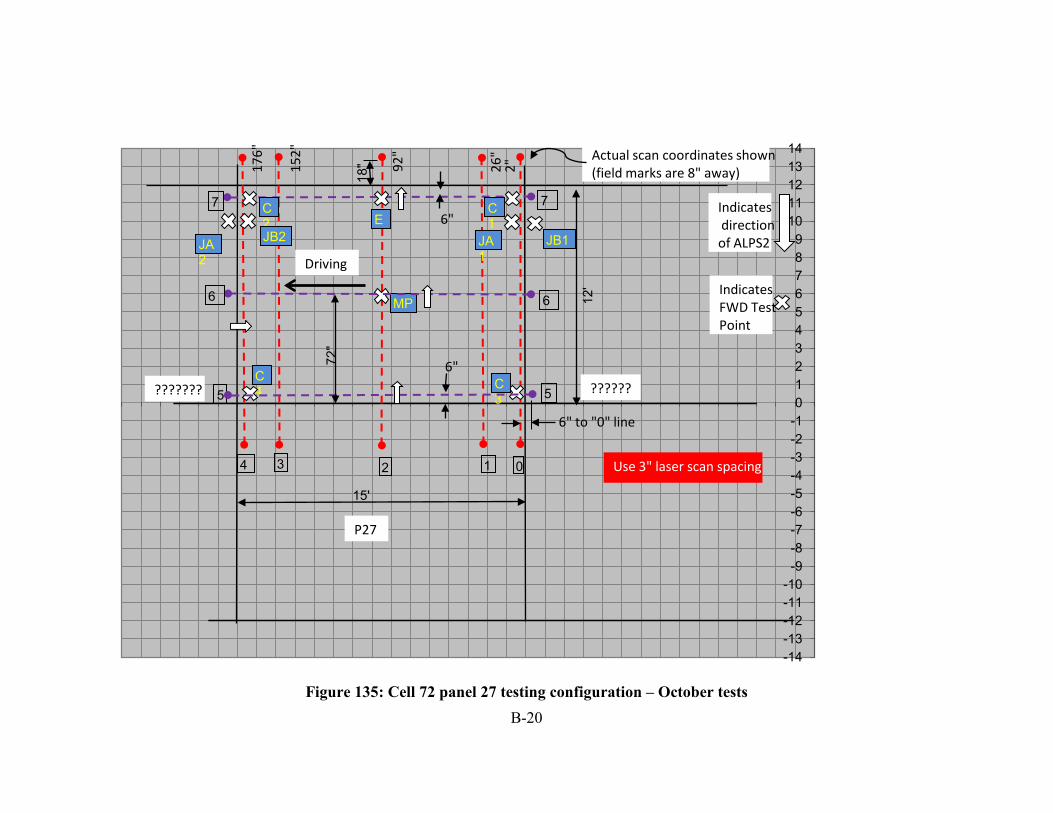
B-20
Figure 135: Cell 72 panel 27 testing configuration – October tests
-14-13-12-11-10-9-8-7-6-5-4-3-2-10123456789
1011121314
1 0234
P27
Driving
5
152"
2"26"
92"
176"
Indicatesdirection of ALPS2
Use 3" laser scan spacing
Actual scan coordinates shown (field marks are 8" away)
5
15'
12'
C2
C1E
C3
C4
MP
JB2JA2
JB1JA1
IndicatesFWD Test Point
7 7
6 6
6" to "0" line
??????? ??????
6"
6"72"
18"
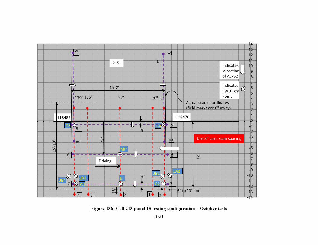
B-21
Figure 136: Cell 213 panel 15 testing configuration – October tests
-14-13-12-11-10-9-8-7-6-5-4-3-2-10123456789
1011121314
0
8
12
118470118485
P15
7
L
15'-2"
12'34
8
99
Indicatesdirection of ALPS2
IndicatesFWD Test Point
JA1JB1C1 C2
C4C3
E
MP
2"155" 92" 26"179"Actual scan coordinates (field marks are 8" away)
JA2JB2
Driving
15'-1
0"
Use 3" laser scan spacing
66
55
7
6" to "0" line
6"
6"
72"
18"
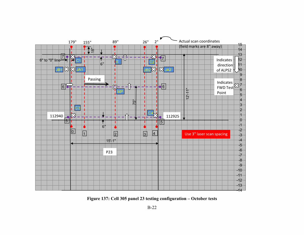
B-22
Figure 137: Cell 305 panel 23 testing configuration – October tests
-14-13-12-11-10-9-8-7-6-5-4-3-2-10123456789
101112131415
43210
112925112940
P23
Passing
7
155" 89" 26"179" 2"
6"Indicatesdirection of ALPS2
Use 3" laser scan spacing
Actual scan coordinates (field marks are 8" away)
15'-1"
12'-1
1"
6" to "0" line 7
IndicatesFWD Test Point
C1
C4C3
MP
C2E
JA1JB1 JA2JB2
55
66
75"
6"
18"

B-23
Figure 138: Cell 513 panel 5 testing configuration – October tests
-14-13-12-11-10-9-8-7-6-5-4-3-2-10123456789
1011121314
0
8
123
118410118422
P5
7
12'
12'
4
8
99
Indicatesdirection of ALPS2
IndicatesFWD Test Point
JA1JB1
C1
C2
C4
C3
E
MP
2"26"140" 71"116"
7
Actual scan coordinates (field marks are 8" away)
JA2JB2
Driving
Use 3" laser scan spacing
55
66
6" to "0" line
6"
6"
69"
18"

B-24
Figure 139: Cell 614 panel 57 testing configuration – October tests
-14-13-12-11-10-9-8-7-6-5-4-3-2-10123456789
1011121314
0123
119253119265
P57
7
12'-2"
12'
4
6"
Indicatesdirection of ALPS2
IndicatesFWD Test Point
JA1JB1
C1 C2
C4C3
E
MP
2"143" 119" 71" 26"
7
Actual scan coordinates (field marks are 8" away)
JA2JB2
Driving
Use 3" laser scan spacing
6
55
6
36"
6"
6"6" to "0" line18
"

APPENDIX C: TEMPERATURE PROFILES

C-1
Table 29: Temperature profiles through depth of slab during FWD testing in June
pavement depth (in)
temp during testing
temp during testing
sensor depth (in)
extrapolate Temp difference
(deg F) cell panel AM/PM trial
top (deg C)
bottom (deg C)
top (deg F)
bottom (deg F) top bottom
top (deg F)
bottom (deg F)
7 12 AM 1 7.1 22.2 21.1 71.96 69.98 0.96 3.96 72.59 67.91 4.69 7 12 PM 1 7.1 36.5 34.1 97.7 93.38 0.96 3.96 99.08 88.86 10.22 7 14 AM 1 7.1 20.67 20.53 69.206 68.954 0.96 3.96 69.29 68.69 0.60 7 14 PM 1 7.1 35.8 34.2 96.44 93.56 0.96 3.96 97.36 90.55 6.82
12 19 AM 1 9.9 20.2 24.1 68.36 75.38 1.2 9 67.28 73.67 -6.39 12 19 AM 2 9.9 20 24 68 75.2 1.2 9.48 66.96 73.13 -6.17 12 19 PM 1 9.9 37 26.5 98.6 79.7 1.2 9 101.51 84.30 17.20 12 19 PM 2 9.9 37.9 27 100.22 80.6 1.2 9.48 103.06 86.24 16.82 12 24 AM 1 9.9 19.9 24.2 67.82 75.56 1.2 9 66.63 73.67 -7.05 12 24 AM 2 9.9 19.8 24 67.64 75.2 1.2 9.48 66.54 73.03 -6.48 12 24 PM 1 9.9 36.7 26.3 98.06 79.34 1.2 9 100.94 83.90 17.04 12 24 PM 2 9.9 37.6 26.2 99.68 79.16 1.2 9.48 102.65 85.06 17.60 36 19 AM 1 6.5 17.8 21.6 64.04 70.88 1.32 6.12 62.16 72.28 -10.12 36 19 PM 1 6.5 36.8 31.9 98.24 89.42 1.32 6.12 100.67 87.62 13.05 36 20 AM 1 6.5 17.8 21.6 64.04 70.88 1.32 6.12 62.16 72.28 -10.12 36 20 PM 1 6.5 36.8 31.9 98.24 89.42 1.32 6.12 100.67 87.62 13.05 37 8 AM 1 6.5 19.1 19.6 66.38 67.28 1.08 3.12 65.90 69.04 -3.13 37 8 PM 1 6.5 37.5 36.1 99.5 96.98 1.08 3.12 100.83 92.06 8.77 37 9 AM 1 6.5 19.1 19.6 66.38 67.28 1.08 3.12 65.90 69.04 -3.13 37 9 PM 1 6.5 37.5 36.1 99.5 96.98 1.08 3.12 100.83 92.06 8.77

C-2
pavement depth (in)
temp during testing temp during
testing sensor
depth (in) extrapolate temp
difference (deg F) cell panel AM/PM trial
top (deg C)
bottom (deg C)
top (deg F)
bottom (deg F)
top bottom top
(deg F) bottom (deg F)
53 3 AM 1 12 19.51 20.44 67.118 68.792 0.504 9 67.02 68.42 -1.40 53 3 AM 2 12 22.05 23.15 71.69 73.67 0.504 9 71.57 73.23 -1.65 53 3 PM 1 12 31.8 26.8 89.24 80.24 0.504 9 89.77 82.25 7.52
53 3 PM 2 12 34.6 24.32 94.28 75.776 0.504 9 95.38 79.91 15.46 205 18 PM 1 4 31.62 30.21 88.916 86.378 0.504 3.996 89.28 84.12 5.16 205 18 PM 2 4 35.4 33.7 95.72 92.66 0.504 3.504 96.23 88.99 7.24 213a 15 AM 1 5.5 18.14 20.7 64.652 69.26 0.504 5.004 64.14 71.41 -7.27
213a 15 PM 1 5.5 34.8 28 94.64 82.4 0.504 5.004 96.01 76.70 19.31 305b 23 AM 1 5 19.17 21.4 66.506 70.52 0.504 3.996 65.93 74.09 -8.16 305 b 23 AM 2 5 20.3 22.4 68.54 72.32 0.504 3.504 67.90 76.85 -8.95 305 b 23 PM 1 5 30.3 28.8 86.54 83.84 0.504 3.996 86.93 81.44 5.49
305 b 23 PM 2 5 34.2 31.8 93.56 89.24 0.504 3.504 94.29 84.06 10.22 313 26 AM 1 6 18.15 20.8 64.67 69.44 0.504 5.004 64.14 71.66 -7.53 313 26 PM 1 6 34 28 93.2 82.4 0.504 5.004 94.41 77.37 17.04
513 a 5 AM 1 5.8 18.4 20.6 65.12 69.08 0.504 5.004 64.68 70.92 -6.25
513 a 5 PM 1 5.8 34.5 28.7 94.1 83.66 0.504 5.004 95.27 78.80 16.47 a thermocouple data was not available for this cell, data from cell 313 was used instead b thermocouple data was not available for this cell, data from cell 205 was used instead

C-3
Table 30: Temperature profiles through depth of slab during ALPS2 testing in October
Pavement depth (in)
Temp during profiling Temp during profiling sensor
depth (in) extrapolate Temp
Difference (deg F)
cell trial time top
(deg C) bottom (deg C)
top (deg F)
bottom (deg F) top bottom top (deg F)
bottom (deg F)
7 1 early 7.1 8.27 11.6 46.886 52.88 1.32 7.32 45.6 52.66 -7.09 7 2 early 7.1 8.65 11.7 47.57 53.06 1.44 7.44 46.3 52.75 -6.50
12 1 early 9.9 8 13 46.4 55.4 1.2 9 45.0 56.44 -11.42 12 1 early 9.9 8.3 13.15 46.94 55.67 1.2 9.48 45.7 56.11 -10.44 36 1 early 6.5 8.5 13 47.3 55.4 1.08 6.24 45.6 55.81 -10.20 36 1 late 6.5 15.8 13.1 60.44 55.58 1.08 6.24 61.5 55.34 6.12 37 1 early 6.5 8.2 12.8 46.76 55.04 1.08 6.24 45.0 55.46 -10.43 37 1 late 6.5 18 13.7 64.4 56.66 1.08 6.24 66.0 56.27 9.75 53 1 early 12 7.5 12.6 45.5 54.68 0.504 9 45.0 57.92 -12.97 53 2 early 12 8 15.78 46.4 60.404 0.504 9 45.6 65.35 -19.78 53 1 late 12 15.2 12.7 59.36 54.86 0.504 9 59.6 53.27 6.36 53 2 late 12 18 14.97 64.4 58.946 0.504 9 64.7 57.02 7.70
305 2 early 5 8 9.7 46.4 49.46 0.504 3.96 46.0 50.38 -4.43 71* 1 early 9 8 13.1 46.4 55.58 1.2 9 45.0 55.58 -10.59 71* 2 early 9 8.2 13.3 46.76 55.94 1.2 9.48 45.4 55.41 -9.98 72* 1 early 9 8 13 46.4 55.4 1.2 9 45.0 55.40 -10.38 72* 2 early 9 8.3 13.2 46.94 55.76 1.2 9.48 45.7 55.25 -9.59
213* 1 early 6 8.5 11.2 47.3 52.16 1.2 9.48 46.6 50.12 -3.52 213* 2 early 6 8.3 11.4 46.94 52.52 1.2 9.48 46.1 50.17 -4.04
513* 1 early 6 8.5 11.2 47.3 52.16 1.2 9.48 46.6 50.12 -3.52 513* 2 early 6 8.3 11.4 46.94 52.52 1.2 9.48 46.1 50.17 -4.04 614* 1 early 6 8.5 11.2 47.3 52.16 1.2 9.48 46.6 50.12 -3.52 614* 2 early 6 8.3 11.4 46.94 52.52 1.2 9.48 46.1 50.17 -4.04
*thermocouple data not available, used data from cell 12 instead
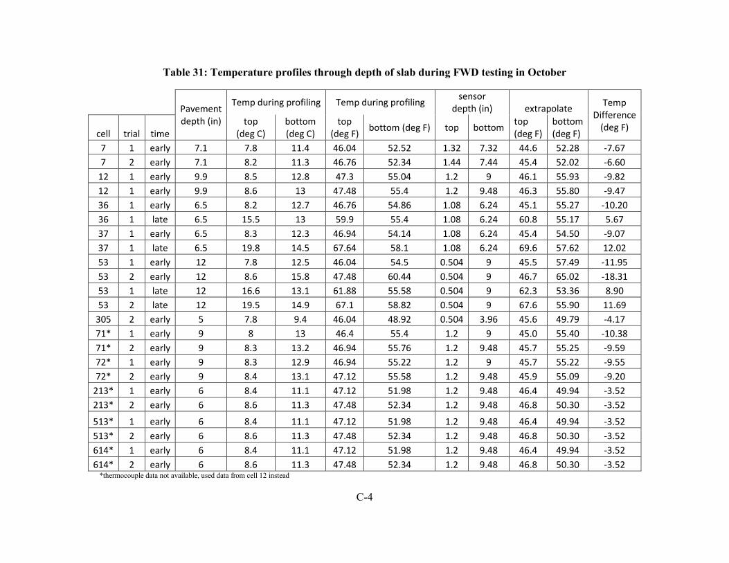
C-4
Table 31: Temperature profiles through depth of slab during FWD testing in October
Pavement depth (in)
Temp during profiling Temp during profiling sensor
depth (in) extrapolate Temp
Difference (deg F)
cell trial time top
(deg C) bottom (deg C)
top (deg F)
bottom (deg F) top bottom top (deg F)
bottom (deg F)
7 1 early 7.1 7.8 11.4 46.04 52.52 1.32 7.32 44.6 52.28 -7.67 7 2 early 7.1 8.2 11.3 46.76 52.34 1.44 7.44 45.4 52.02 -6.60
12 1 early 9.9 8.5 12.8 47.3 55.04 1.2 9 46.1 55.93 -9.82 12 1 early 9.9 8.6 13 47.48 55.4 1.2 9.48 46.3 55.80 -9.47 36 1 early 6.5 8.2 12.7 46.76 54.86 1.08 6.24 45.1 55.27 -10.20 36 1 late 6.5 15.5 13 59.9 55.4 1.08 6.24 60.8 55.17 5.67 37 1 early 6.5 8.3 12.3 46.94 54.14 1.08 6.24 45.4 54.50 -9.07 37 1 late 6.5 19.8 14.5 67.64 58.1 1.08 6.24 69.6 57.62 12.02 53 1 early 12 7.8 12.5 46.04 54.5 0.504 9 45.5 57.49 -11.95 53 2 early 12 8.6 15.8 47.48 60.44 0.504 9 46.7 65.02 -18.31 53 1 late 12 16.6 13.1 61.88 55.58 0.504 9 62.3 53.36 8.90 53 2 late 12 19.5 14.9 67.1 58.82 0.504 9 67.6 55.90 11.69
305 2 early 5 7.8 9.4 46.04 48.92 0.504 3.96 45.6 49.79 -4.17 71* 1 early 9 8 13 46.4 55.4 1.2 9 45.0 55.40 -10.38 71* 2 early 9 8.3 13.2 46.94 55.76 1.2 9.48 45.7 55.25 -9.59 72* 1 early 9 8.3 12.9 46.94 55.22 1.2 9 45.7 55.22 -9.55 72* 2 early 9 8.4 13.1 47.12 55.58 1.2 9.48 45.9 55.09 -9.20
213* 1 early 6 8.4 11.1 47.12 51.98 1.2 9.48 46.4 49.94 -3.52 213* 2 early 6 8.6 11.3 47.48 52.34 1.2 9.48 46.8 50.30 -3.52
513* 1 early 6 8.4 11.1 47.12 51.98 1.2 9.48 46.4 49.94 -3.52 513* 2 early 6 8.6 11.3 47.48 52.34 1.2 9.48 46.8 50.30 -3.52 614* 1 early 6 8.4 11.1 47.12 51.98 1.2 9.48 46.4 49.94 -3.52 614* 2 early 6 8.6 11.3 47.48 52.34 1.2 9.48 46.8 50.30 -3.52
*thermocouple data not available, used data from cell 12 instead

APPENDIX D: ISLAB2000 INPUT PARAMETERS
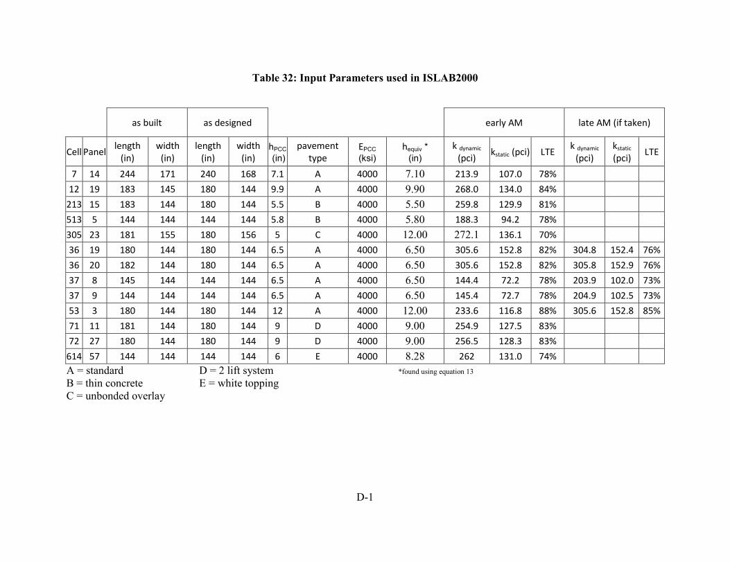
D-1
Table 32: Input Parameters used in ISLAB2000
as built as designed
early AM late AM (if taken)
Cell Panel length
(in) width
(in) length
(in) width
(in) hPCC (in)
pavement type
EPCC
(ksi) hequiv *
(in) k dynamic
(pci) kstatic (pci) LTE
k dynamic (pci)
kstatic (pci)
LTE
7 14 244 171 240 168 7.1 A 4000 7.10 213.9 107.0 78%
12 19 183 145 180 144 9.9 A 4000 9.90 268.0 134.0 84%
213 15 183 144 180 144 5.5 B 4000 5.50 259.8 129.9 81%
513 5 144 144 144 144 5.8 B 4000 5.80 188.3 94.2 78%
305 23 181 155 180 156 5 C 4000 12.00 272.1 136.1 70%
36 19 180 144 180 144 6.5 A 4000 6.50 305.6 152.8 82% 304.8 152.4 76%
36 20 182 144 180 144 6.5 A 4000 6.50 305.6 152.8 82% 305.8 152.9 76%
37 8 145 144 144 144 6.5 A 4000 6.50 144.4 72.2 78% 203.9 102.0 73%
37 9 144 144 144 144 6.5 A 4000 6.50 145.4 72.7 78% 204.9 102.5 73%
53 3 180 144 180 144 12 A 4000 12.00 233.6 116.8 88% 305.6 152.8 85%
71 11 181 144 180 144 9 D 4000 9.00 254.9 127.5 83%
72 27 180 144 180 144 9 D 4000 9.00 256.5 128.3 83%
614 57 144 144 144 144 6 E 4000 8.28 262 131.0 74%
A = standard D = 2 lift system *found using equation 13 B = thin concrete E = white topping C = unbonded overlay

APPENDIX E: ACTUAL DATA WITH ISLAB2000 CURVE MATCHED VIA THE POLYNOMIAL CURVATURE METHOD

E-1
4.15
4.2
4.25
4.3
4.35
4.4
4.45
4.5
0 10 20 30 40 50 60 70
Diff
eren
ce b
etw
een
refe
renc
e pl
ane
and
slab
su
rfae
(in)
Along transverse length of slab
pass 0 actual
pass 1 actual
pass 2 actual
pass 3 actual
pass 4 actual
pass 0 ISLAB
pass 1 ISLAB
pass 2 ISLAB
pass 3 ISLAB
pass 4 ISLAB
Figure 140: Cell 7 actual data and ISLAB2000 curve from the 2nd order polynomial approximation
Figure 141: Cell 7 actual data and ISLAB2000 curve from the 3rd order polynomial
approximation
4.15
4.2
4.25
4.3
4.35
4.4
4.45
4.5
0 20 40 60 80Diff
eren
ce b
etw
een
refe
renc
e pl
ane
and
slab
sur
face
(in)
Along transverse length of slab
pass 0 actual
pass 1 actual
pass 2 actual
pass 3 actual
pass 4 actual
pass 0 ISLAB
pass 1 ISLAB
pass 2 ISLAB
pass 3 ISLAB
pass 4 ISLAB

E-2
Figure 142: Cell 7 actual data and ISLAB2000 curve from the 4th order polynomial
approximation
Figure 143: Cell 7 actual data and ISLAB2000 curve from the 5th order polynomial
approximation
4.15
4.2
4.25
4.3
4.35
4.4
4.45
4.5
0 20 40 60 80
Diff
eren
ce b
etw
een
refe
renc
e pl
ane
and
slab
su
rfac
e (in
)
Along transverse length of slab
pass 0 actual
pass 1 actual
pass 2 actual
pass 3 actual
pass 4 actual
pass 0 ISLAB
pass 1 ISLAB
pass 2 ISLAB
pass 3 ISLAB
pass 4 ISLAB
4.15
4.2
4.25
4.3
4.35
4.4
4.45
4.5
4.55
0 20 40 60 80
Diff
eren
ce b
etw
een
refe
renc
e pl
ane
and
slab
su
rfac
e (in
)
Along transverse length of slab
pass 0 actual
pass 1 actual
pass 2 actual
pass 3 actual
pass 4 actual
pass 0 ISLAB
pass 1 ISLAB
pass 2 ISLAB
pass 3 ISLAB
pass 4 ISLAB
Note: ISLAB2000 profile could not be matched to passes 0, 1, 2, 3, or 4

E-3
Figure 144: Cell 7 actual data and ISLAB2000 curve from the 6th order polynomial
approximation
Figure 145: Cell 12 actual data and ISLAB2000 curve from the 2nd order polynomial
approximation
4.15
4.2
4.25
4.3
4.35
4.4
4.45
4.5
0 20 40 60 80
Diff
eren
tial
Def
lect
ion
betw
een
Slab
and
D
atum
(in)
Along transverse length of slab
pass 0 actual
pass 1 actual
pass 2 actual
pass 3 actual
pass 4 actual
pass 0 ISLAB
pass 1 ISLAB
pass 2 ISLAB
pass 3 ISLAB
pass 4 ISLAB
3.75
3.8
3.85
3.9
3.95
4
4.05
4.1
4.15
0 10 20 30 40 50 60 70
Diff
eren
ce b
etw
een
refe
renc
e pl
ane
and
slab
su
rfae
(in)
Along transverse length of slab
pass 0 actual
pass 1 actual
pass 2 actual
pass 3 actual
pass 4 actual
pass 0 ISLAB
pass 1 ISLAB
pass 2 ISLAB
pass 3 ISLAB
pass 4 ISLAB
Note: ISLAB2000 profile could not be matched to passes 0, 1, 2, 3, or 4
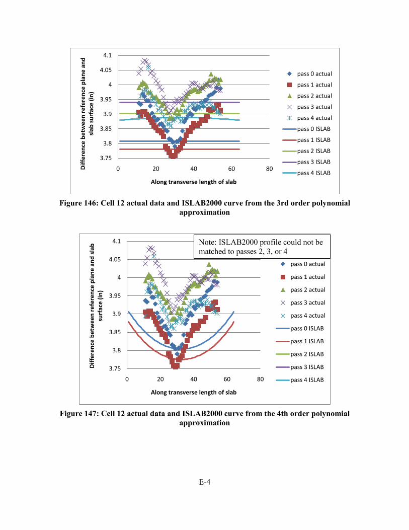
E-4
Figure 146: Cell 12 actual data and ISLAB2000 curve from the 3rd order polynomial
approximation
Figure 147: Cell 12 actual data and ISLAB2000 curve from the 4th order polynomial
approximation
3.75
3.8
3.85
3.9
3.95
4
4.05
4.1
0 20 40 60 80Diff
eren
ce b
etw
een
refe
renc
e pl
ane
and
slab
sur
face
(in)
Along transverse length of slab
pass 0 actual
pass 1 actual
pass 2 actual
pass 3 actual
pass 4 actual
pass 0 ISLAB
pass 1 ISLAB
pass 2 ISLAB
pass 3 ISLAB
pass 4 ISLAB
3.75
3.8
3.85
3.9
3.95
4
4.05
4.1
0 20 40 60 80
Diff
eren
ce b
etw
een
refe
renc
e pl
ane
and
slab
su
rfac
e (in
)
Along transverse length of slab
pass 0 actual
pass 1 actual
pass 2 actual
pass 3 actual
pass 4 actual
pass 0 ISLAB
pass 1 ISLAB
pass 2 ISLAB
pass 3 ISLAB
pass 4 ISLAB
Note: ISLAB2000 profile could not be matched to passes 2, 3, or 4
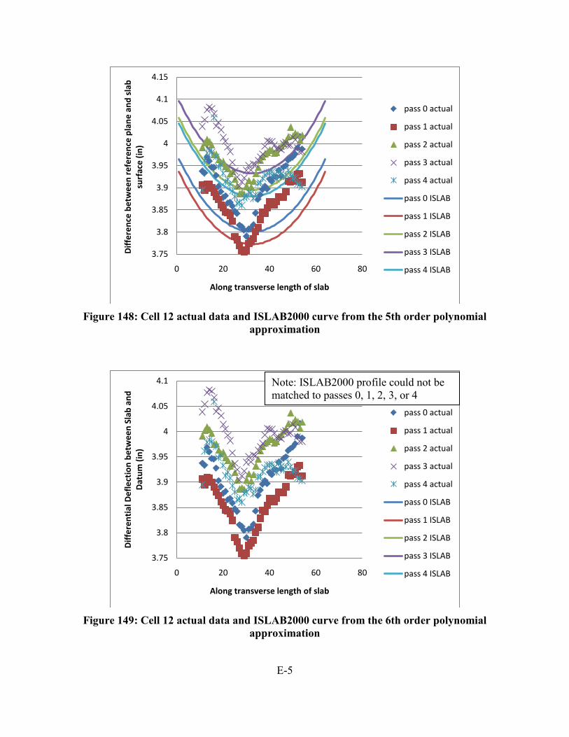
E-5
Figure 148: Cell 12 actual data and ISLAB2000 curve from the 5th order polynomial
approximation
Figure 149: Cell 12 actual data and ISLAB2000 curve from the 6th order polynomial
approximation
3.75
3.8
3.85
3.9
3.95
4
4.05
4.1
4.15
0 20 40 60 80
Diff
eren
ce b
etw
een
refe
renc
e pl
ane
and
slab
su
rfac
e (in
)
Along transverse length of slab
pass 0 actual
pass 1 actual
pass 2 actual
pass 3 actual
pass 4 actual
pass 0 ISLAB
pass 1 ISLAB
pass 2 ISLAB
pass 3 ISLAB
pass 4 ISLAB
3.75
3.8
3.85
3.9
3.95
4
4.05
4.1
0 20 40 60 80
Diff
eren
tial
Def
lect
ion
betw
een
Slab
and
D
atum
(in)
Along transverse length of slab
pass 0 actual
pass 1 actual
pass 2 actual
pass 3 actual
pass 4 actual
pass 0 ISLAB
pass 1 ISLAB
pass 2 ISLAB
pass 3 ISLAB
pass 4 ISLAB
Note: ISLAB2000 profile could not be matched to passes 0, 1, 2, 3, or 4
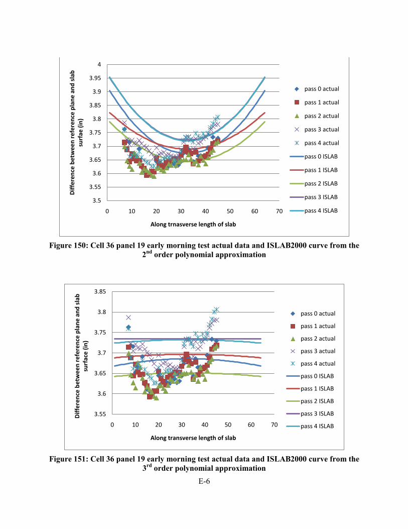
E-6
Figure 150: Cell 36 panel 19 early morning test actual data and ISLAB2000 curve from the
2nd order polynomial approximation
Figure 151: Cell 36 panel 19 early morning test actual data and ISLAB2000 curve from the
3rd order polynomial approximation
3.5
3.55
3.6
3.65
3.7
3.75
3.8
3.85
3.9
3.95
4
0 10 20 30 40 50 60 70
Diff
eren
ce b
etw
een
refe
renc
e pl
ane
and
slab
su
rfae
(in)
Along trnasverse length of slab
pass 0 actual
pass 1 actual
pass 2 actual
pass 3 actual
pass 4 actual
pass 0 ISLAB
pass 1 ISLAB
pass 2 ISLAB
pass 3 ISLAB
pass 4 ISLAB
3.55
3.6
3.65
3.7
3.75
3.8
3.85
0 10 20 30 40 50 60 70
Diff
eren
ce b
etw
een
refe
renc
e pl
ane
and
slab
su
rfac
e (in
)
Along transverse length of slab
pass 0 actual
pass 1 actual
pass 2 actual
pass 3 actual
pass 4 actual
pass 0 ISLAB
pass 1 ISLAB
pass 2 ISLAB
pass 3 ISLAB
pass 4 ISLAB
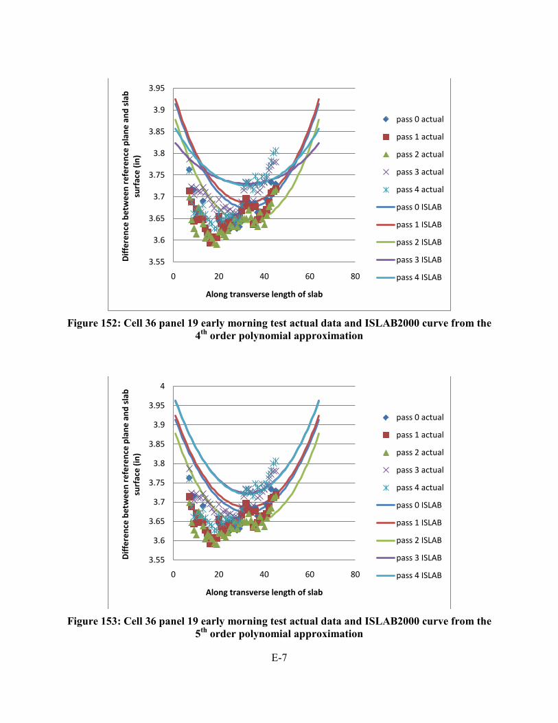
E-7
Figure 152: Cell 36 panel 19 early morning test actual data and ISLAB2000 curve from the
4th order polynomial approximation
Figure 153: Cell 36 panel 19 early morning test actual data and ISLAB2000 curve from the
5th order polynomial approximation
3.55
3.6
3.65
3.7
3.75
3.8
3.85
3.9
3.95
0 20 40 60 80
Diff
eren
ce b
etw
een
refe
renc
e pl
ane
and
slab
su
rfac
e (in
)
Along transverse length of slab
pass 0 actual
pass 1 actual
pass 2 actual
pass 3 actual
pass 4 actual
pass 0 ISLAB
pass 1 ISLAB
pass 2 ISLAB
pass 3 ISLAB
pass 4 ISLAB
3.55
3.6
3.65
3.7
3.75
3.8
3.85
3.9
3.95
4
0 20 40 60 80
Diff
eren
ce b
etw
een
refe
renc
e pl
ane
and
slab
su
rfac
e (in
)
Along transverse length of slab
pass 0 actual
pass 1 actual
pass 2 actual
pass 3 actual
pass 4 actual
pass 0 ISLAB
pass 1 ISLAB
pass 2 ISLAB
pass 3 ISLAB
pass 4 ISLAB
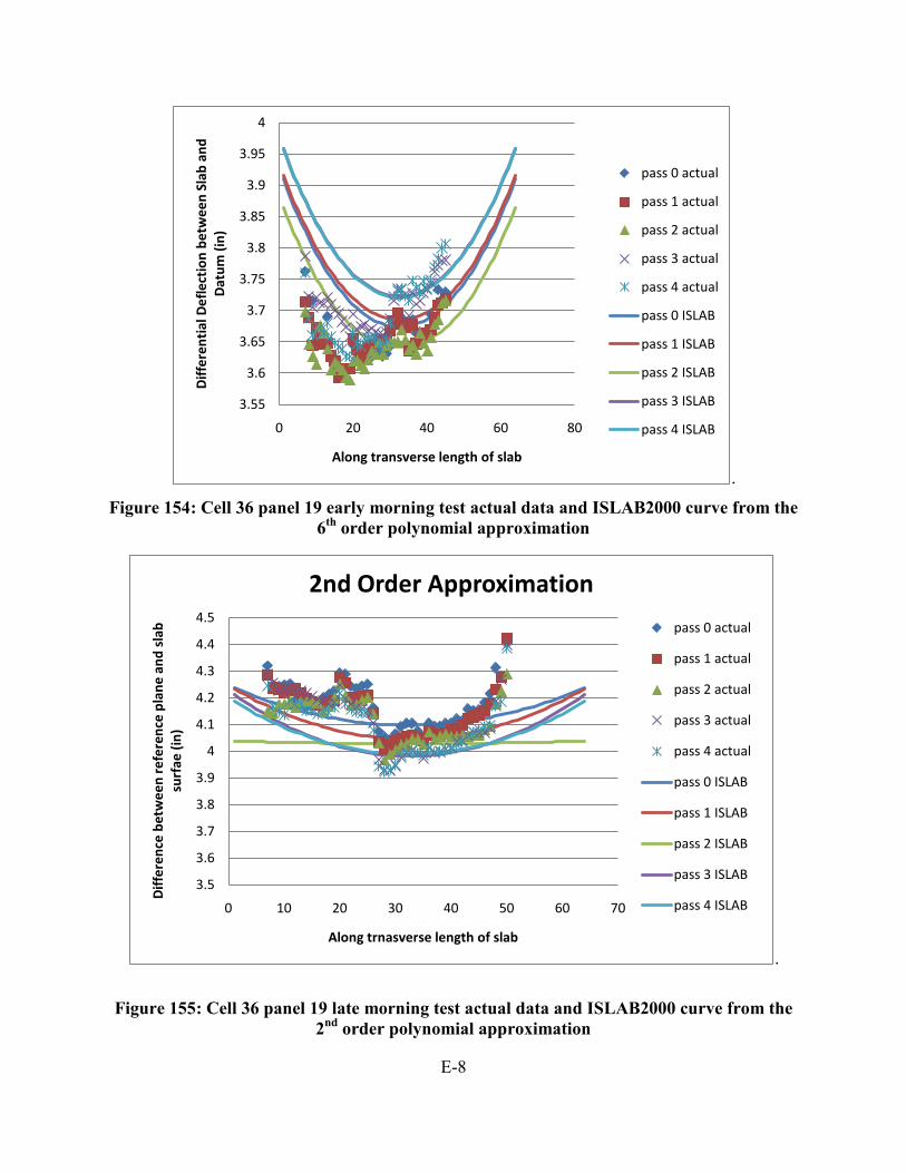
E-8
.
Figure 154: Cell 36 panel 19 early morning test actual data and ISLAB2000 curve from the 6th order polynomial approximation
.
Figure 155: Cell 36 panel 19 late morning test actual data and ISLAB2000 curve from the 2nd order polynomial approximation
3.55
3.6
3.65
3.7
3.75
3.8
3.85
3.9
3.95
4
0 20 40 60 80
Diff
eren
tial
Def
lect
ion
betw
een
Slab
and
D
atum
(in)
Along transverse length of slab
pass 0 actual
pass 1 actual
pass 2 actual
pass 3 actual
pass 4 actual
pass 0 ISLAB
pass 1 ISLAB
pass 2 ISLAB
pass 3 ISLAB
pass 4 ISLAB
3.5
3.6
3.7
3.8
3.9
4
4.1
4.2
4.3
4.4
4.5
0 10 20 30 40 50 60 70
Diff
eren
ce b
etw
een
refe
renc
e pl
ane
and
slab
su
rfae
(in)
Along trnasverse length of slab
2nd Order Approximation
pass 0 actual
pass 1 actual
pass 2 actual
pass 3 actual
pass 4 actual
pass 0 ISLAB
pass 1 ISLAB
pass 2 ISLAB
pass 3 ISLAB
pass 4 ISLAB

E-9
Figure 156: Cell 36 panel 19 late morning test actual data and ISLAB2000 curve from the
3rd order polynomial approximation
Figure 157: Cell 36 panel 19 late morning test actual data and ISLAB2000 curve from the
4th order polynomial approximation
3.9
4
4.1
4.2
4.3
4.4
4.5
0 20 40 60 80
Diff
eren
ce b
etw
een
refe
renc
e pl
ane
and
slab
sur
face
(in
)
Along transverse length of slab
pass 0 actual
pass 1 actual
pass 2 actual
pass 3 actual
pass 4 actual
pass 0 ISLAB
pass 1 ISLAB
pass 2 ISLAB
pass 3 ISLAB
pass 4 ISLAB
3.9
4
4.1
4.2
4.3
4.4
4.5
0 20 40 60 80
Diff
eren
ce b
etw
een
refe
renc
e pl
ane
and
slab
su
rfac
e (in
)
Along transverse length of slab
pass 0 actual
pass 1 actual
pass 2 actual
pass 3 actual
pass 4 actual
pass 0 ISLAB
pass 1 ISLAB
pass 2 ISLAB
pass 3 ISLAB
pass 4 ISLAB
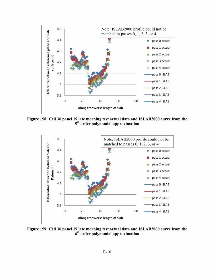
E-10
Figure 158: Cell 36 panel 19 late morning test actual data and ISLAB2000 curve from the
5th order polynomial approximation
Figure 159: Cell 36 panel 19 late morning test actual data and ISLAB2000 curve from the
6th order polynomial approximation
3.9
4
4.1
4.2
4.3
4.4
4.5
0 20 40 60 80
Diff
eren
ce b
etw
een
refe
renc
e pl
ane
and
slab
su
rfac
e (in
)
Along transverse length of slab
pass 0 actual
pass 1 actual
pass 2 actual
pass 3 actual
pass 4 actual
pass 0 ISLAB
pass 1 ISLAB
pass 2 ISLAB
pass 3 ISLAB
pass 4 ISLAB
3.9
4
4.1
4.2
4.3
4.4
4.5
0 20 40 60 80
Diff
eren
tial
Def
lect
ion
betw
een
Slab
and
D
atum
(in)
Along transverse length of slab
pass 0 actual
pass 1 actual
pass 2 actual
pass 3 actual
pass 4 actual
pass 0 ISLAB
pass 1 ISLAB
pass 2 ISLAB
pass 3 ISLAB
pass 4 ISLAB
Note: ISLAB2000 profile could not be matched to passes 0, 1, 2, 3, or 4
Note: ISLAB2000 profile could not be matched to passes 0, 1, 2, 3, or 4

E-11
.
Figure 160: Cell 36 panel 20 early morning test actual data and ISLAB2000 curve from the 2nd order polynomial approximation
Figure 161: Cell 36 panel 20 early morning test actual data and ISLAB2000 curve from the
3rd order polynomial approximation
3.5
3.55
3.6
3.65
3.7
3.75
3.8
0 10 20 30 40 50 60 70
Diff
eren
ce b
etw
een
refe
renc
e pl
ane
and
slab
su
rfae
(in)
Along transverse length of slab
pass 0 actual
pass 1 actual
pass 2 actual
pass 3 actual
pass 4 actual
pass 0 ISLAB
pass 1 ISLAB
pass 2 ISLAB
pass 3 ISLAB
pass 4 ISLAB
3.4
3.45
3.5
3.55
3.6
3.65
3.7
3.75
3.8
0 10 20 30 40 50 60 70
Diff
eren
ce b
etw
een
refe
renc
e pl
ane
and
slab
su
rfac
e (in
)
Along transverse length of slab
pass 0 actual
pass 1 actual
pass 2 actual
pass 3 actual
pass 4 actual
pass 0 ISLAB
pass 1 ISLAB
pass 2 ISLAB
pass 3 ISLAB
pass 4 ISLAB
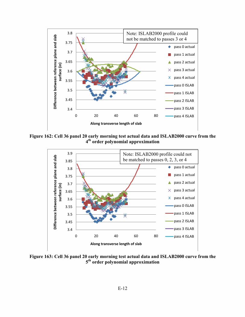
E-12
Figure 162: Cell 36 panel 20 early morning test actual data and ISLAB2000 curve from the
4th order polynomial approximation
Figure 163: Cell 36 panel 20 early morning test actual data and ISLAB2000 curve from the
5th order polynomial approximation
3.4
3.45
3.5
3.55
3.6
3.65
3.7
3.75
3.8
0 20 40 60 80
Diff
eren
ce b
etw
een
refe
renc
e pl
ane
and
slab
su
rfac
e (in
)
Along transverse length of slab
pass 0 actual
pass 1 actual
pass 2 actual
pass 3 actual
pass 4 actual
pass 0 ISLAB
pass 1 ISLAB
pass 2 ISLAB
pass 3 ISLAB
pass 4 ISLAB
3.4
3.45
3.5
3.55
3.6
3.65
3.7
3.75
3.8
3.85
3.9
0 20 40 60 80
Diff
eren
ce b
etw
een
refe
renc
e pl
ane
and
slab
su
rfac
e (in
)
Along transverse length of slab
pass 0 actual
pass 1 actual
pass 2 actual
pass 3 actual
pass 4 actual
pass 0 ISLAB
pass 1 ISLAB
pass 2 ISLAB
pass 3 ISLAB
pass 4 ISLAB
Note: ISLAB2000 profile could not be matched to passes 3 or 4
Note: ISLAB2000 profile could not be matched to passes 0, 2, 3, or 4
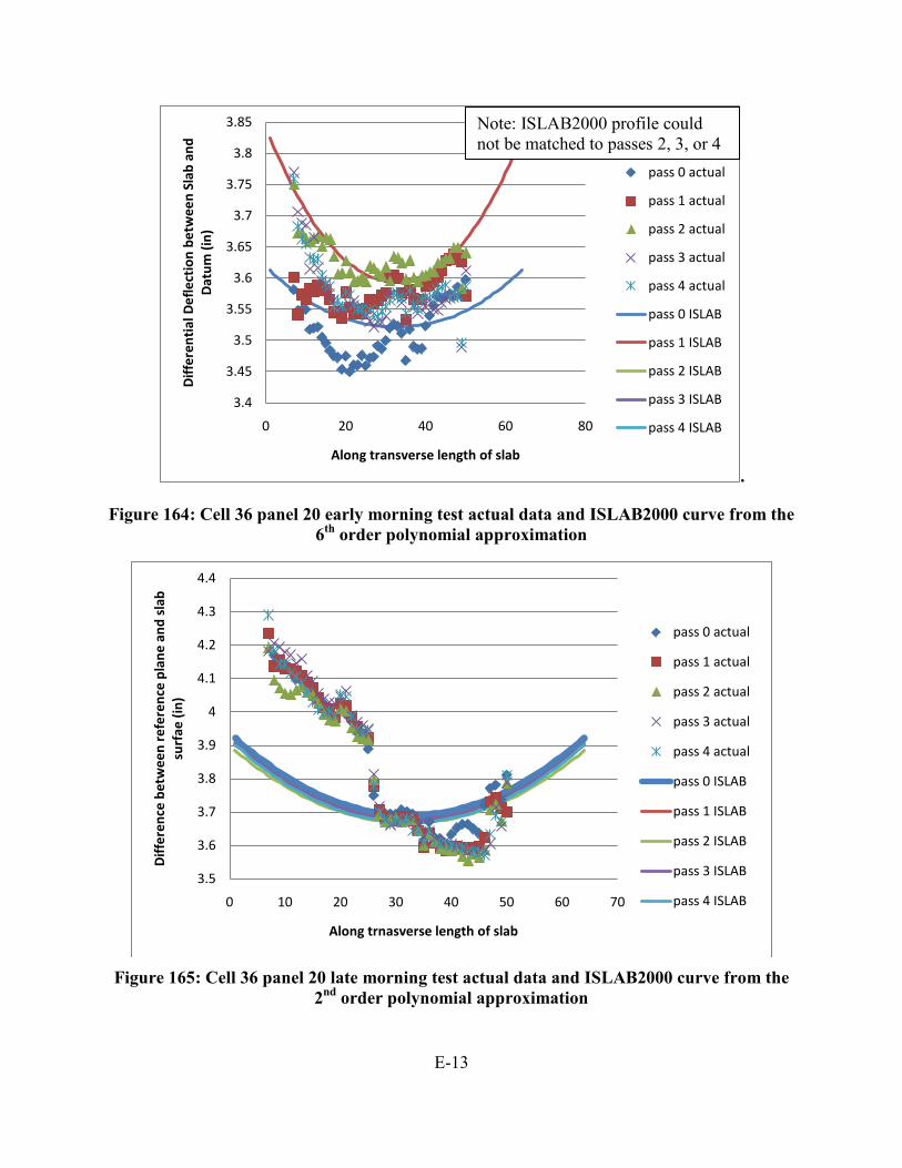
E-13
.
Figure 164: Cell 36 panel 20 early morning test actual data and ISLAB2000 curve from the 6th order polynomial approximation
Figure 165: Cell 36 panel 20 late morning test actual data and ISLAB2000 curve from the
2nd order polynomial approximation
3.4
3.45
3.5
3.55
3.6
3.65
3.7
3.75
3.8
3.85
0 20 40 60 80
Diff
eren
tial
Def
lect
ion
betw
een
Slab
and
D
atum
(in)
Along transverse length of slab
pass 0 actual
pass 1 actual
pass 2 actual
pass 3 actual
pass 4 actual
pass 0 ISLAB
pass 1 ISLAB
pass 2 ISLAB
pass 3 ISLAB
pass 4 ISLAB
3.5
3.6
3.7
3.8
3.9
4
4.1
4.2
4.3
4.4
0 10 20 30 40 50 60 70
Diff
eren
ce b
etw
een
refe
renc
e pl
ane
and
slab
su
rfae
(in)
Along trnasverse length of slab
pass 0 actual
pass 1 actual
pass 2 actual
pass 3 actual
pass 4 actual
pass 0 ISLAB
pass 1 ISLAB
pass 2 ISLAB
pass 3 ISLAB
pass 4 ISLAB
Note: ISLAB2000 profile could not be matched to passes 2, 3, or 4

E-14
Figure 166: Cell 36 panel 20 late morning test actual data and ISLAB2000 curve from the
3rd order polynomial approximation
.
Figure 167: Cell 36 panel 20 late morning test actual data and ISLAB2000 curve from the 4th order polynomial approximation
3.5
3.6
3.7
3.8
3.9
4
4.1
4.2
4.3
4.4
0 20 40 60 80
Diff
eren
ce b
etw
een
refe
renc
e pl
ane
and
slab
su
rfac
e (in
)
Along transverse length of slab
pass 0 actual
pass 1 actual
pass 2 actual
pass 3 actual
pass 4 actual
pass 0 ISLAB
pass 1 ISLAB
pass 2 ISLAB
pass 3 ISLAB
pass 4 ISLAB
3.5
3.6
3.7
3.8
3.9
4
4.1
4.2
4.3
4.4
0 20 40 60 80
Diff
eren
ce b
etw
een
refe
renc
e pl
ane
and
slab
su
rfac
e (in
)
Along transverse length of slab
pass 0 actual
pass 1 actual
pass 2 actual
pass 3 actual
pass 4 actual
pass 0 ISLAB
pass 1 ISLAB
pass 2 ISLAB
pass 3 ISLAB
pass 4 ISLAB
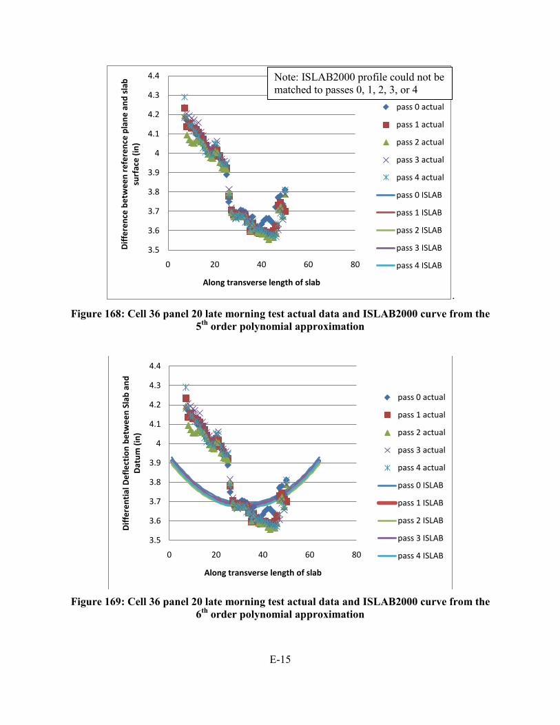
E-15
.
Figure 168: Cell 36 panel 20 late morning test actual data and ISLAB2000 curve from the 5th order polynomial approximation
Figure 169: Cell 36 panel 20 late morning test actual data and ISLAB2000 curve from the
6th order polynomial approximation
3.5
3.6
3.7
3.8
3.9
4
4.1
4.2
4.3
4.4
0 20 40 60 80
Diff
eren
ce b
etw
een
refe
renc
e pl
ane
and
slab
su
rfac
e (in
)
Along transverse length of slab
pass 0 actual
pass 1 actual
pass 2 actual
pass 3 actual
pass 4 actual
pass 0 ISLAB
pass 1 ISLAB
pass 2 ISLAB
pass 3 ISLAB
pass 4 ISLAB
3.5
3.6
3.7
3.8
3.9
4
4.1
4.2
4.3
4.4
0 20 40 60 80
Diff
eren
tial
Def
lect
ion
betw
een
Slab
and
D
atum
(in)
Along transverse length of slab
pass 0 actual
pass 1 actual
pass 2 actual
pass 3 actual
pass 4 actual
pass 0 ISLAB
pass 1 ISLAB
pass 2 ISLAB
pass 3 ISLAB
pass 4 ISLAB
Note: ISLAB2000 profile could not be matched to passes 0, 1, 2, 3, or 4
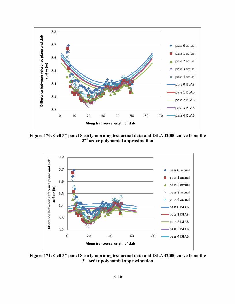
E-16
Figure 170: Cell 37 panel 8 early morning test actual data and ISLAB2000 curve from the
2nd order polynomial approximation
Figure 171: Cell 37 panel 8 early morning test actual data and ISLAB2000 curve from the
3rd order polynomial approximation
3.2
3.3
3.4
3.5
3.6
3.7
3.8
0 10 20 30 40 50 60 70
Diff
eren
ce b
etw
een
refe
renc
e pl
ane
and
slab
su
rfae
(in)
Along transverse length of slab
pass 0 actual
pass 1 actual
pass 2 actual
pass 3 actual
pass 4 actual
pass 0 ISLAB
pass 1 ISLAB
pass 2 ISLAB
pass 3 ISLAB
pass 4 ISLAB
3.2
3.3
3.4
3.5
3.6
3.7
3.8
0 20 40 60 80
Diff
eren
ce b
etw
een
refe
renc
e pl
ane
and
slab
su
rfac
e (in
)
Along transverse length of slab
pass 0 actual
pass 1 actual
pass 2 actual
pass 3 actual
pass 4 actual
pass 0 ISLAB
pass 1 ISLAB
pass 2 ISLAB
pass 3 ISLAB
pass 4 ISLAB

E-17
Figure 172: Cell 37 panel 8 early morning test actual data and ISLAB2000 curve from the
4th order polynomial approximation
Figure 173: Cell 37 panel 8 early morning test actual data and ISLAB2000 curve from the
5th order polynomial approximation
3.2
3.3
3.4
3.5
3.6
3.7
3.8
0 20 40 60 80
Diff
eren
ce b
etw
een
refe
renc
e pl
ane
and
slab
su
rfac
e (in
)
Along transverse length of slab
pass 0 actual
pass 1 actual
pass 2 actual
pass 3 actual
pass 4 actual
pass 0 ISLAB
pass 1 ISLAB
pass 2 ISLAB
pass 3 ISLAB
pass 4 ISLAB
3.2
3.3
3.4
3.5
3.6
3.7
3.8
0 20 40 60 80
Diff
eren
ce b
etw
een
refe
renc
e pl
ane
and
slab
su
rfac
e (in
)
Along transverse length of slab
pass 0 actual
pass 1 actual
pass 2 actual
pass 3 actual
pass 4 actual
pass 0 ISLAB
pass 1 ISLAB
pass 2 ISLAB
pass 3 ISLAB
pass 4 ISLAB
Note: ISLAB2000 profile could not be matched to passes 0, 1, 2, or 4
Note: ISLAB2000 profile could not be matched to passes 0, 1, 2, 3, or 4
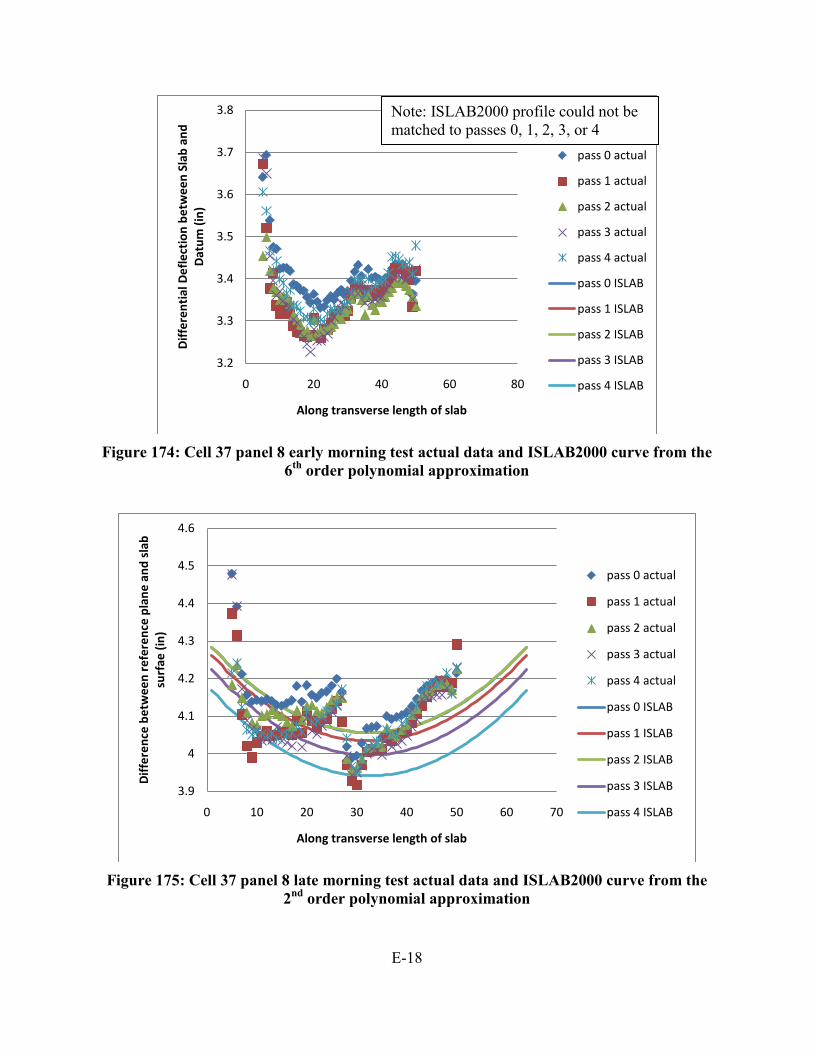
E-18
Figure 174: Cell 37 panel 8 early morning test actual data and ISLAB2000 curve from the
6th order polynomial approximation
Figure 175: Cell 37 panel 8 late morning test actual data and ISLAB2000 curve from the
2nd order polynomial approximation
3.2
3.3
3.4
3.5
3.6
3.7
3.8
0 20 40 60 80
Diff
eren
tial
Def
lect
ion
betw
een
Slab
and
D
atum
(in)
Along transverse length of slab
pass 0 actual
pass 1 actual
pass 2 actual
pass 3 actual
pass 4 actual
pass 0 ISLAB
pass 1 ISLAB
pass 2 ISLAB
pass 3 ISLAB
pass 4 ISLAB
3.9
4
4.1
4.2
4.3
4.4
4.5
4.6
0 10 20 30 40 50 60 70
Diff
eren
ce b
etw
een
refe
renc
e pl
ane
and
slab
su
rfae
(in)
Along transverse length of slab
pass 0 actual
pass 1 actual
pass 2 actual
pass 3 actual
pass 4 actual
pass 0 ISLAB
pass 1 ISLAB
pass 2 ISLAB
pass 3 ISLAB
pass 4 ISLAB
Note: ISLAB2000 profile could not be matched to passes 0, 1, 2, 3, or 4

E-19
Figure 176: Cell 37 panel 8 late morning test actual data and ISLAB2000 curve from the
3rd order polynomial approximation
Figure 177: Cell 37 panel 8 late morning test actual data and ISLAB2000 curve from the 4th
order polynomial approximation
3.5
3.7
3.9
4.1
4.3
4.5
4.7
0 10 20 30 40 50 60 70
Diff
eren
ce b
etw
een
refe
renc
e pl
ane
and
slab
su
rfae
(in)
Along trnasverse length of slab
pass 0 actual
pass 1 actual
pass 2 actual
pass 3 actual
pass 4 actual
pass 0 ISLAB
pass 1 ISLAB
pass 2 ISLAB
pass 3 ISLAB
pass 4 ISLAB
3.9
4
4.1
4.2
4.3
4.4
4.5
4.6
0 20 40 60 80
Diff
eren
ce b
etw
een
refe
renc
e pl
ane
and
slab
su
rfac
e (in
)
Along transverse length of slab
pass 0 actual
pass 1 actual
pass 2 actual
pass 3 actual
pass 4 actual
pass 0 ISLAB
pass 1 ISLAB
pass 2 ISLAB
pass 3 ISLAB
pass 4 ISLAB
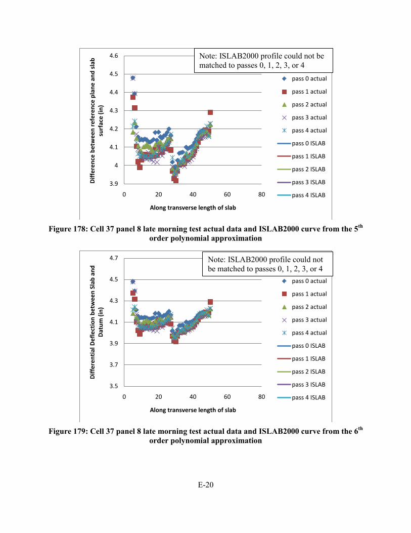
E-20
Figure 178: Cell 37 panel 8 late morning test actual data and ISLAB2000 curve from the 5th
order polynomial approximation
Figure 179: Cell 37 panel 8 late morning test actual data and ISLAB2000 curve from the 6th
order polynomial approximation
3.9
4
4.1
4.2
4.3
4.4
4.5
4.6
0 20 40 60 80
Diff
eren
ce b
etw
een
refe
renc
e pl
ane
and
slab
su
rfac
e (in
)
Along transverse length of slab
pass 0 actual
pass 1 actual
pass 2 actual
pass 3 actual
pass 4 actual
pass 0 ISLAB
pass 1 ISLAB
pass 2 ISLAB
pass 3 ISLAB
pass 4 ISLAB
3.5
3.7
3.9
4.1
4.3
4.5
4.7
0 20 40 60 80
Diff
eren
tial
Def
lect
ion
betw
een
Slab
and
D
atum
(in)
Along transverse length of slab
pass 0 actual
pass 1 actual
pass 2 actual
pass 3 actual
pass 4 actual
pass 0 ISLAB
pass 1 ISLAB
pass 2 ISLAB
pass 3 ISLAB
pass 4 ISLAB
Note: ISLAB2000 profile could not be matched to passes 0, 1, 2, 3, or 4
Note: ISLAB2000 profile could not be matched to passes 0, 1, 2, 3, or 4

E-21
Figure 180: Cell 37 panel 9 early morning test actual data and ISLAB2000 curve from the
2nd order polynomial approximation
Figure 181: Cell 37 panel 9 early morning test actual data and ISLAB2000 curve from the
3rd order polynomial approximation
3.2
3.3
3.4
3.5
3.6
3.7
3.8
0 10 20 30 40 50 60 70
Diff
eren
ce b
etw
een
refe
renc
e pl
ane
and
slab
su
rfae
(in)
Along transverse length of slab
pass 0 actual
pass 1 actual
pass 2 actual
pass 3 actual
pass 4 actual
pass 0 ISLAB
pass 1 ISLAB
pass 2 ISLAB
pass 3 ISLAB
pass 4 ISLAB
3.2
3.3
3.4
3.5
3.6
3.7
3.8
0 20 40 60 80
Diff
eren
ce b
etw
een
refe
renc
e pl
ane
and
slab
su
rfac
e (in
)
Along transverse length of slab
pass 0 actual
pass 1 actual
pass 2 actual
pass 3 actual
pass 4 actual
pass 0 ISLAB
pass 1 ISLAB
pass 2 ISLAB
pass 3 ISLAB
pass 4 ISLAB
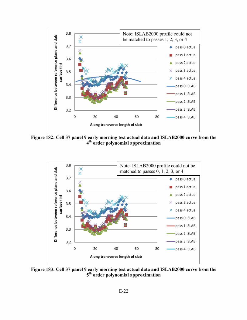
E-22
Figure 182: Cell 37 panel 9 early morning test actual data and ISLAB2000 curve from the
4th order polynomial approximation
Figure 183: Cell 37 panel 9 early morning test actual data and ISLAB2000 curve from the
5th order polynomial approximation
3.2
3.3
3.4
3.5
3.6
3.7
3.8
0 20 40 60 80
Diff
eren
ce b
etw
een
refe
renc
e pl
ane
and
slab
su
rfac
e (in
)
Along transverse length of slab
pass 0 actual
pass 1 actual
pass 2 actual
pass 3 actual
pass 4 actual
pass 0 ISLAB
pass 1 ISLAB
pass 2 ISLAB
pass 3 ISLAB
pass 4 ISLAB
3.2
3.3
3.4
3.5
3.6
3.7
3.8
0 20 40 60 80
Diff
eren
ce b
etw
een
refe
renc
e pl
ane
and
slab
su
rfac
e (in
)
Along transverse length of slab
pass 0 actual
pass 1 actual
pass 2 actual
pass 3 actual
pass 4 actual
pass 0 ISLAB
pass 1 ISLAB
pass 2 ISLAB
pass 3 ISLAB
pass 4 ISLAB
Note: ISLAB2000 profile could not be matched to passes 1, 2, 3, or 4
Note: ISLAB2000 profile could not be matched to passes 0, 1, 2, 3, or 4

E-23
Figure 184: Cell 37 panel 9 early morning test actual data and ISLAB2000 curve from the
6th order polynomial approximation
Figure 185: Cell 37 panel 9 late morning test actual data and ISLAB2000 curve from the
2nd order polynomial approximation
3.2
3.3
3.4
3.5
3.6
3.7
3.8
0 20 40 60 80
Diff
eren
tial
Def
lect
ion
betw
een
Slab
and
D
atum
(in)
Along transverse length of slab
pass 0 actual
pass 1 actual
pass 2 actual
pass 3 actual
pass 4 actual
pass 0 ISLAB
pass 1 ISLAB
pass 2 ISLAB
pass 3 ISLAB
pass 4 ISLAB
3.9
4
4.1
4.2
4.3
4.4
4.5
4.6
0 10 20 30 40 50 60 70
Diff
eren
ce b
etw
een
refe
renc
e pl
ane
and
slab
sur
fae
(in)
Along trnasverse length of slab
pass 0 actual
pass 1 actual
pass 2 actual
pass 3 actual
pass 4 actual
pass 0 ISLAB
pass 1 ISLAB
pass 2 ISLAB
pass 3 ISLAB
pass 4 ISLAB
Note: ISLAB2000 profile could not be matched to passes 0, 1, 2, 3, or 4

E-24
Figure 186: Cell 37 panel 9 late morning test actual data and ISLAB2000 curve from the
3rd order polynomial approximation
Figure 187: Cell 37 panel 9 late morning test actual data and ISLAB2000 curve from the 4th
order polynomial approximation
3.9
4
4.1
4.2
4.3
4.4
4.5
4.6
0 20 40 60 80
Diff
eren
ce b
etw
een
refe
renc
e pl
ane
and
slab
su
rfac
e (in
)
Along transverse length of slab
pass 0 actual
pass 1 actual
pass 2 actual
pass 3 actual
pass 4 actual
pass 0 ISLAB
pass 1 ISLAB
pass 2 ISLAB
pass 3 ISLAB
pass 4 ISLAB
3.9
4
4.1
4.2
4.3
4.4
4.5
4.6
0 20 40 60 80
Diff
eren
ce b
etw
een
refe
renc
e pl
ane
and
slab
su
rfac
e (in
)
Along transverse length of slab
pass 0 actual
pass 1 actual
pass 2 actual
pass 3 actual
pass 4 actual
pass 0 ISLAB
pass 1 ISLAB
pass 2 ISLAB
pass 3 ISLAB
pass 4 ISLAB

E-25
Figure 188: Cell 37 panel 9 late morning test actual data and ISLAB2000 curve from the 5th
order polynomial approximation
Figure 189: Cell 37 panel 9 late morning test actual data and ISLAB2000 curve from the 6th
order polynomial approximation
3.9
4
4.1
4.2
4.3
4.4
4.5
4.6
0 20 40 60 80
Diff
eren
ce b
etw
een
refe
renc
e pl
ane
and
slab
su
rfac
e (in
)
Along transverse length of slab
pass 0 actual
pass 1 actual
pass 2 actual
pass 3 actual
pass 4 actual
pass 0 ISLAB
pass 1 ISLAB
pass 2 ISLAB
pass 3 ISLAB
pass 4 ISLAB
3.9
4
4.1
4.2
4.3
4.4
4.5
4.6
0 20 40 60 80
Diff
eren
ce b
etw
een
refe
renc
e pl
ane
and
slab
su
rfac
e (in
)
Along transverse length of slab
pass 0 actual
pass 1 actual
pass 2 actual
pass 3 actual
pass 4 actual
pass 0 ISLAB
pass 1 ISLAB
pass 2 ISLAB
pass 3 ISLAB
pass 4 ISLAB
Note: ISLAB2000 profile could not be matched to passes 0, 1, 2, 3, or 4
Note: ISLAB2000 profile could not be matched to passes 0, 1, 2, 3, or 4
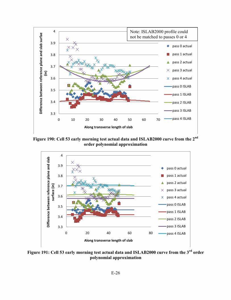
E-26
Figure 190: Cell 53 early morning test actual data and ISLAB2000 curve from the 2nd
order polynomial approximation
Figure 191: Cell 53 early morning test actual data and ISLAB2000 curve from the 3rd order
polynomial approximation
3.3
3.4
3.5
3.6
3.7
3.8
3.9
4
0 10 20 30 40 50 60 70
Diff
eren
ce b
etw
een
refe
renc
e pl
ane
and
slab
sur
fae
(in)
Along transverse length of slab
pass 0 actual
pass 1 actual
pass 2 actual
pass 3 actual
pass 4 actual
pass 0 ISLAB
pass 1 ISLAB
pass 2 ISLAB
pass 3 ISLAB
pass 4 ISLAB
3.3
3.4
3.5
3.6
3.7
3.8
3.9
4
0 20 40 60 80
Diff
eren
ce b
etw
een
refe
renc
e pl
ane
and
slab
su
rfac
e (in
)
Along transverse length of slab
pass 0 actual
pass 1 actual
pass 2 actual
pass 3 actual
pass 4 actual
pass 0 ISLAB
pass 1 ISLAB
pass 2 ISLAB
pass 3 ISLAB
pass 4 ISLAB
Note: ISLAB2000 profile could not be matched to passes 0 or 4
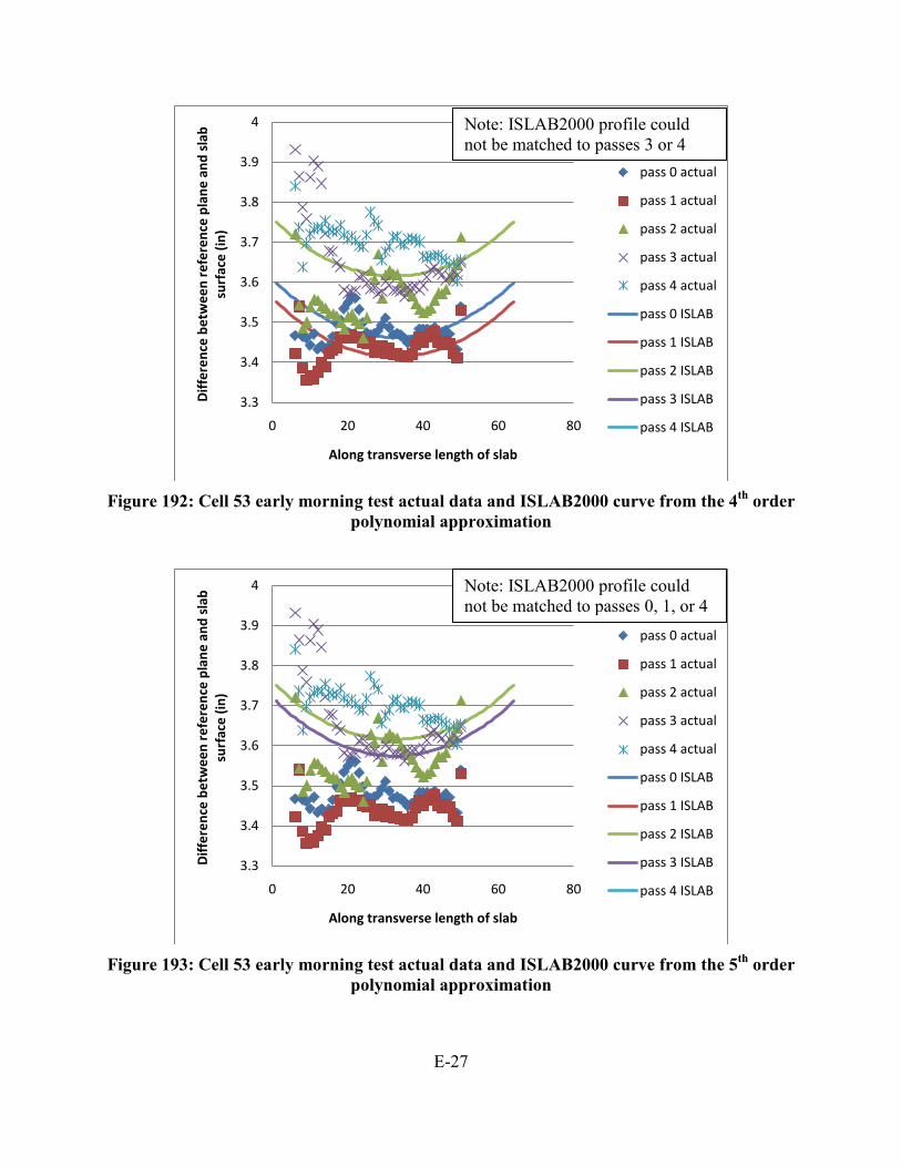
E-27
Figure 192: Cell 53 early morning test actual data and ISLAB2000 curve from the 4th order
polynomial approximation
Figure 193: Cell 53 early morning test actual data and ISLAB2000 curve from the 5th order
polynomial approximation
3.3
3.4
3.5
3.6
3.7
3.8
3.9
4
0 20 40 60 80
Diff
eren
ce b
etw
een
refe
renc
e pl
ane
and
slab
su
rfac
e (in
)
Along transverse length of slab
pass 0 actual
pass 1 actual
pass 2 actual
pass 3 actual
pass 4 actual
pass 0 ISLAB
pass 1 ISLAB
pass 2 ISLAB
pass 3 ISLAB
pass 4 ISLAB
3.3
3.4
3.5
3.6
3.7
3.8
3.9
4
0 20 40 60 80
Diff
eren
ce b
etw
een
refe
renc
e pl
ane
and
slab
su
rfac
e (in
)
Along transverse length of slab
pass 0 actual
pass 1 actual
pass 2 actual
pass 3 actual
pass 4 actual
pass 0 ISLAB
pass 1 ISLAB
pass 2 ISLAB
pass 3 ISLAB
pass 4 ISLAB
Note: ISLAB2000 profile could not be matched to passes 3 or 4
Note: ISLAB2000 profile could not be matched to passes 0, 1, or 4

E-28
Figure 194: Cell 53 early morning test actual data and ISLAB2000 curve from the 6th order
polynomial approximation
Figure 195: Cell 53 late morning test actual data and ISLAB2000 curve from the 2nd order
polynomial approximation
3.3
3.4
3.5
3.6
3.7
3.8
3.9
4
0 20 40 60 80
Diff
eren
tial
Def
lect
ion
betw
een
Slab
and
D
atum
(in)
Along transverse length of slab
pass 0 actual
pass 1 actual
pass 2 actual
pass 3 actual
pass 4 actual
pass 0 ISLAB
pass 1 ISLAB
pass 2 ISLAB
pass 3 ISLAB
pass 4 ISLAB
4.1
4.2
4.3
4.4
4.5
4.6
4.7
4.8
4.9
0 10 20 30 40 50 60 70
Diff
eren
ce b
etw
een
refe
renc
e pl
ane
and
slab
su
rfae
(in)
Along transverse length of slab
pass 0 actual
pass 1 actual
pass 2 actual
pass 3 actual
pass 4 actual
pass 0 ISLAB
pass 1 ISLAB
pass 2 ISLAB
pass 3 ISLAB
pass 4 ISLAB
Note: ISLAB2000 profile could not be matched to passes 0, 1, or 4
Note: ISLAB2000 profile could not be matched to passes 0 or 4

E-29
Figure 196: Cell 53 late morning test actual data and ISLAB2000 curve from the 3rd order
polynomial approximation
Figure 197: Cell 53 late morning test actual data and ISLAB2000 curve from the 4th order
polynomial approximation
4.1
4.2
4.3
4.4
4.5
4.6
4.7
4.8
4.9
0 20 40 60 80
Diff
eren
ce b
etw
een
refe
renc
e pl
ane
and
slab
su
rfac
e (in
)
Along transverse length of slab
pass 0 actual
pass 1 actual
pass 2 actual
pass 3 actual
pass 4 actual
pass 0 ISLAB
pass 1 ISLAB
pass 2 ISLAB
pass 3 ISLAB
pass 4 ISLAB
4.1
4.2
4.3
4.4
4.5
4.6
4.7
4.8
4.9
0 20 40 60 80
Diff
eren
ce b
etw
een
refe
renc
e pl
ane
and
slab
su
rfac
e (in
)
Along transverse length of slab
pass 0 actual
pass 1 actual
pass 2 actual
pass 3 actual
pass 4 actual
pass 0 ISLAB
pass 1 ISLAB
pass 2 ISLAB
pass 3 ISLAB
pass 4 ISLAB

E-30
Figure 198: Cell 53 late morning test actual data and ISLAB2000 curve from the 5th order
polynomial approximation
Figure 199: Cell 53 late morning test actual data and ISLAB2000 curve from the 6th order
polynomial approximation
4.1
4.2
4.3
4.4
4.5
4.6
4.7
4.8
4.9
0 20 40 60 80Diff
eren
ce b
etw
een
refe
renc
e pl
ane
and
slab
su
rfac
e (in
)
Along transverse length of slab
pass 0 actual
pass 1 actual
pass 2 actual
pass 3 actual
pass 4 actual
pass 0 ISLAB
pass 1 ISLAB
pass 2 ISLAB
pass 3 ISLAB
pass 4 ISLAB
4.1
4.2
4.3
4.4
4.5
4.6
4.7
4.8
4.9
0 20 40 60 80
Diff
eren
tial
Def
lect
ion
betw
een
Slab
and
D
atum
(in)
Along transverse length of slab
pass 0 actual
pass 1 actual
pass 2 actual
pass 3 actual
pass 4 actual
pass 0 ISLAB
pass 1 ISLAB
pass 2 ISLAB
pass 3 ISLAB
pass 4 ISLAB
Note: ISLAB2000 profile could not be matched to passes 0, 1, or 4

E-31
Figure 200: Cell 71 actual data and ISLAB2000 curve from the 2nd order polynomial
approximation
Figure 201: Cell 71 actual data and ISLAB2000 curve from the 3rd order polynomial
approximation
3.15
3.2
3.25
3.3
3.35
3.4
3.45
3.5
3.55
3.6
0 10 20 30 40 50 60 70
Diff
eren
ce b
etw
een
refe
renc
e pl
ane
and
slab
sur
fae
(in)
Along transverse length of slab
pass 0 actual
pass 1 actual
pass 2 actual
pass 3 actual
pass 4 actual
pass 0 ISLAB
pass 1 ISLAB
pass 2 ISLAB
pass 3 ISLAB
pass 4 ISLAB
3.15
3.2
3.25
3.3
3.35
3.4
3.45
3.5
3.55
0 20 40 60 80
Diff
eren
ce b
etw
een
refe
renc
e pl
ane
and
slab
su
rfac
e (in
)
Along transverse length of slab
pass 0 actual
pass 1 actual
pass 2 actual
pass 3 actual
pass 4 actual
pass 0 ISLAB
pass 1 ISLAB
pass 2 ISLAB
pass 3 ISLAB
pass 4 ISLAB
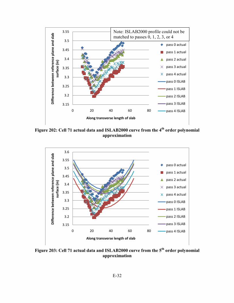
E-32
Figure 202: Cell 71 actual data and ISLAB2000 curve from the 4th order polynomial
approximation
Figure 203: Cell 71 actual data and ISLAB2000 curve from the 5th order polynomial
approximation
3.15
3.2
3.25
3.3
3.35
3.4
3.45
3.5
3.55
0 20 40 60 80
Diff
eren
ce b
etw
een
refe
renc
e pl
ane
and
slab
su
rfac
e (in
)
Along transverse length of slab
pass 0 actual
pass 1 actual
pass 2 actual
pass 3 actual
pass 4 actual
pass 0 ISLAB
pass 1 ISLAB
pass 2 ISLAB
pass 3 ISLAB
pass 4 ISLAB
3.15
3.2
3.25
3.3
3.35
3.4
3.45
3.5
3.55
3.6
0 20 40 60 80
Diff
eren
ce b
etw
een
refe
renc
e pl
ane
and
slab
su
rfac
e (in
)
Along transverse length of slab
pass 0 actual
pass 1 actual
pass 2 actual
pass 3 actual
pass 4 actual
pass 0 ISLAB
pass 1 ISLAB
pass 2 ISLAB
pass 3 ISLAB
pass 4 ISLAB
Note: ISLAB2000 profile could not be matched to passes 0, 1, 2, 3, or 4
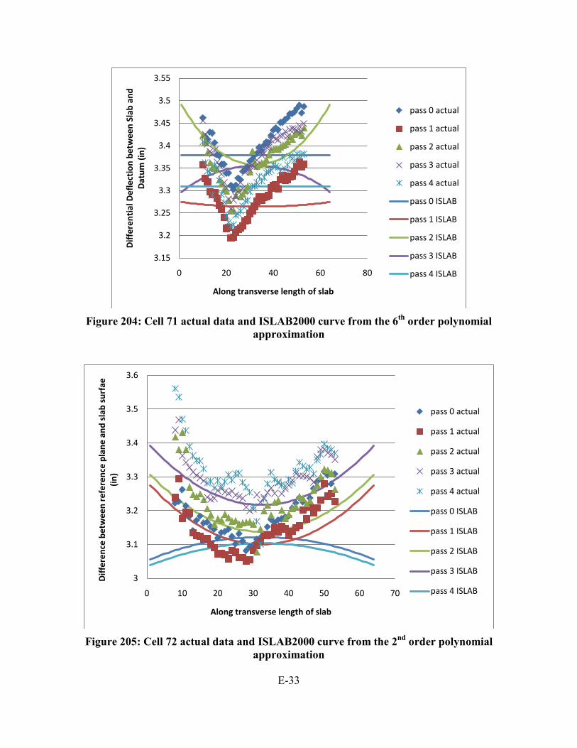
E-33
Figure 204: Cell 71 actual data and ISLAB2000 curve from the 6th order polynomial
approximation
Figure 205: Cell 72 actual data and ISLAB2000 curve from the 2nd order polynomial
approximation
3.15
3.2
3.25
3.3
3.35
3.4
3.45
3.5
3.55
0 20 40 60 80
Diff
eren
tial
Def
lect
ion
betw
een
Slab
and
D
atum
(in)
Along transverse length of slab
pass 0 actual
pass 1 actual
pass 2 actual
pass 3 actual
pass 4 actual
pass 0 ISLAB
pass 1 ISLAB
pass 2 ISLAB
pass 3 ISLAB
pass 4 ISLAB
3
3.1
3.2
3.3
3.4
3.5
3.6
0 10 20 30 40 50 60 70
Diff
eren
ce b
etw
een
refe
renc
e pl
ane
and
slab
sur
fae
(in)
Along transverse length of slab
pass 0 actual
pass 1 actual
pass 2 actual
pass 3 actual
pass 4 actual
pass 0 ISLAB
pass 1 ISLAB
pass 2 ISLAB
pass 3 ISLAB
pass 4 ISLAB

E-34
Figure 206: Cell 72 actual data and ISLAB2000 curve from the 3rd order polynomial
approximation
Figure 207: Cell 72 actual data and ISLAB2000 curve from the 4th order polynomial
approximation
3
3.1
3.2
3.3
3.4
3.5
3.6
0 10 20 30 40 50 60 70
Diff
eren
ce b
etw
een
refe
renc
e pl
ane
and
slab
su
rfac
e (in
)
Along transverse length of slab
pass 0 actual
pass 1 actual
pass 2 actual
pass 3 actual
pass 4 actual
pass 0 ISLAB
pass 1 ISLAB
pass 2 ISLAB
pass 3 ISLAB
pass 4 ISLAB
3
3.1
3.2
3.3
3.4
3.5
3.6
0 20 40 60 80
Diff
eren
ce b
etw
een
refe
renc
e pl
ane
and
slab
su
rfac
e (in
)
Along transverse length of slab
pass 0 actual
pass 1 actual
pass 2 actual
pass 3 actual
pass 4 actual
pass 0 ISLAB
pass 1 ISLAB
pass 2 ISLAB
pass 3 ISLAB
pass 4 ISLAB

E-35
Figure 208: Cell 72 actual data and ISLAB2000 curve from the 5th order polynomial
approximation
Figure 209: Cell 72 actual data and ISLAB2000 curve from the 6th order polynomial
approximation
3
3.1
3.2
3.3
3.4
3.5
3.6
0 20 40 60 80
Diff
eren
ce b
etw
een
refe
renc
e pl
ane
and
slab
su
rfac
e (in
)
Along transverse length of slab
pass 0 actual
pass 1 actual
pass 2 actual
pass 3 actual
pass 4 actual
pass 0 ISLAB
pass 1 ISLAB
pass 2 ISLAB
pass 3 ISLAB
pass 4 ISLAB
3
3.1
3.2
3.3
3.4
3.5
3.6
0 10 20 30 40 50 60 70
Diff
eren
tial
Def
lect
ion
betw
een
Slab
and
D
atum
(in)
Along transverse length of slab
pass 0 actual
pass 1 actual
pass 2 actual
pass 3 actual
pass 4 actual
pass 0 ISLAB
pass 1 ISLAB
pass 2 ISLAB
pass 3 ISLAB
pass 4 ISLAB
Note: ISLAB2000 profile could not be matched to passes 2, 3, or 4
Note: ISLAB2000 profile could not be matched to passes 0 or 4

E-36
Figure 210: Cell 213 actual data and ISLAB2000 curve from the 2nd order polynomial
approximation
Figure 211: Cell 213 actual data and ISLAB2000 curve from the 3rd order polynomial
approximation
3.4
3.5
3.6
3.7
3.8
3.9
4
0 10 20 30 40 50 60 70
Diff
eren
ce b
etw
een
refe
renc
e pl
ane
and
slab
su
rfae
(in)
Along transverse length of slab
pass 0 actual
pass 1 actual
pass 2 actual
pass 3 actual
pass 4 actual
pass 0 ISLAB
pass 1 ISLAB
pass 2 ISLAB
pass 3 ISLAB
pass 4 ISLAB
3.4
3.45
3.5
3.55
3.6
3.65
3.7
3.75
3.8
3.85
3.9
0 20 40 60 80
Diff
eren
ce b
etw
een
refe
renc
e pl
ane
and
slab
su
rfac
e (in
)
Along transverse length of slab
pass 0 actual
pass 1 actual
pass 2 actual
pass 3 actual
pass 4 actual
pass 0 ISLAB
pass 1 ISLAB
pass 2 ISLAB
pass 3 ISLAB
pass 4 ISLAB

E-37
Figure 212: Cell 213 actual data and ISLAB2000 curve from the 4th order polynomial
approximation
Figure 213: Cell 213 actual data and ISLAB2000 curve from the 5th order polynomial
approximation
3.4
3.45
3.5
3.55
3.6
3.65
3.7
3.75
3.8
3.85
3.9
0 20 40 60 80
Diff
eren
ce b
etw
een
refe
renc
e pl
ane
and
slab
su
rfac
e (in
)
Along transverse length of slab
pass 0 actual
pass 1 actual
pass 2 actual
pass 3 actual
pass 4 actual
pass 0 ISLAB
pass 1 ISLAB
pass 2 ISLAB
pass 3 ISLAB
pass 4 ISLAB
3.4
3.45
3.5
3.55
3.6
3.65
3.7
3.75
3.8
3.85
3.9
0 20 40 60 80
Diff
eren
ce b
etw
een
refe
renc
e pl
ane
and
slab
su
rfac
e (in
)
Along transverse length of slab
pass 0 actual
pass 1 actual
pass 2 actual
pass 3 actual
pass 4 actual
pass 0 ISLAB
pass 1 ISLAB
pass 2 ISLAB
pass 3 ISLAB
pass 4 ISLAB
Note: ISLAB2000 profile could not be matched to passes 0, 3, or 4
Note: ISLAB2000 profile could not be matched to passes 0, 1, 2, 3, or 4
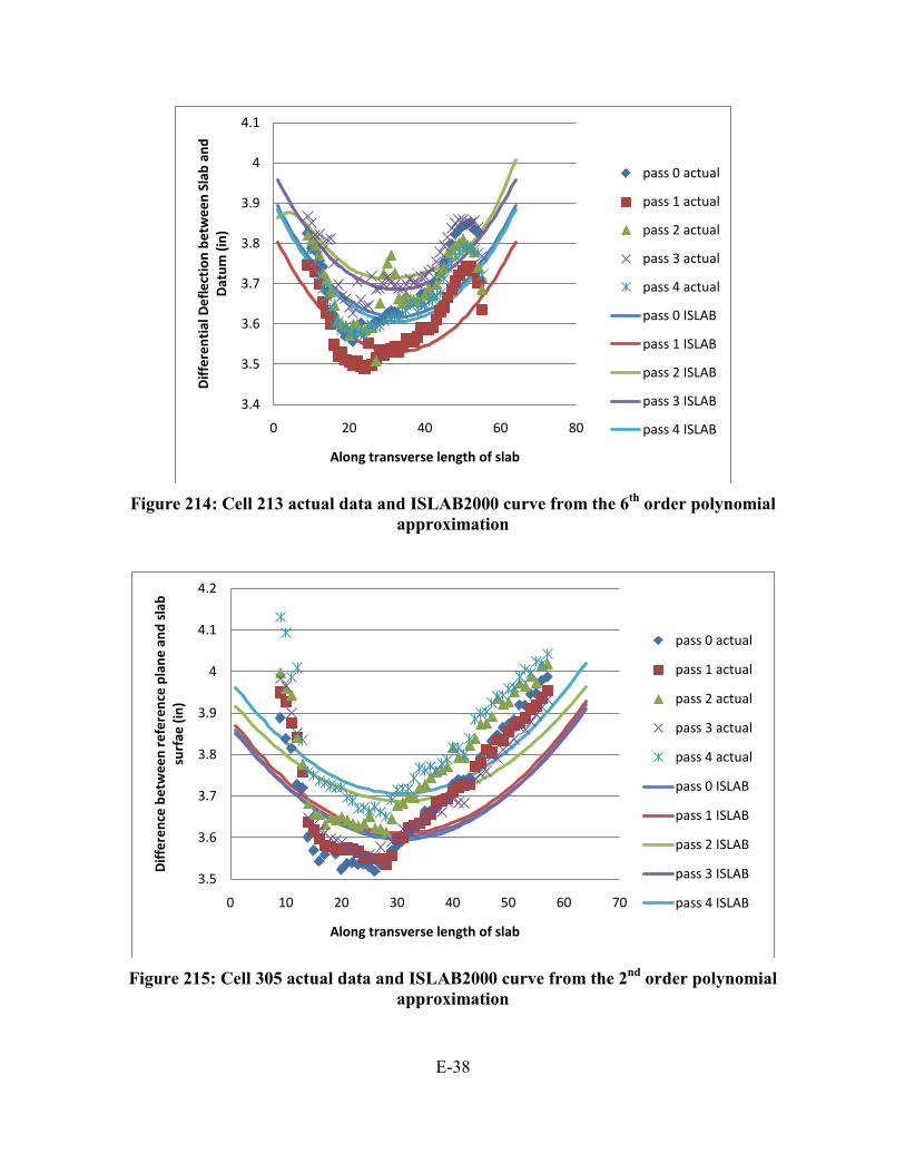
E-38
Figure 214: Cell 213 actual data and ISLAB2000 curve from the 6th order polynomial
approximation
Figure 215: Cell 305 actual data and ISLAB2000 curve from the 2nd order polynomial
approximation
3.4
3.5
3.6
3.7
3.8
3.9
4
4.1
0 20 40 60 80
Diff
eren
tial
Def
lect
ion
betw
een
Slab
and
D
atum
(in)
Along transverse length of slab
pass 0 actual
pass 1 actual
pass 2 actual
pass 3 actual
pass 4 actual
pass 0 ISLAB
pass 1 ISLAB
pass 2 ISLAB
pass 3 ISLAB
pass 4 ISLAB
3.5
3.6
3.7
3.8
3.9
4
4.1
4.2
0 10 20 30 40 50 60 70
Diff
eren
ce b
etw
een
refe
renc
e pl
ane
and
slab
su
rfae
(in)
Along transverse length of slab
pass 0 actual
pass 1 actual
pass 2 actual
pass 3 actual
pass 4 actual
pass 0 ISLAB
pass 1 ISLAB
pass 2 ISLAB
pass 3 ISLAB
pass 4 ISLAB
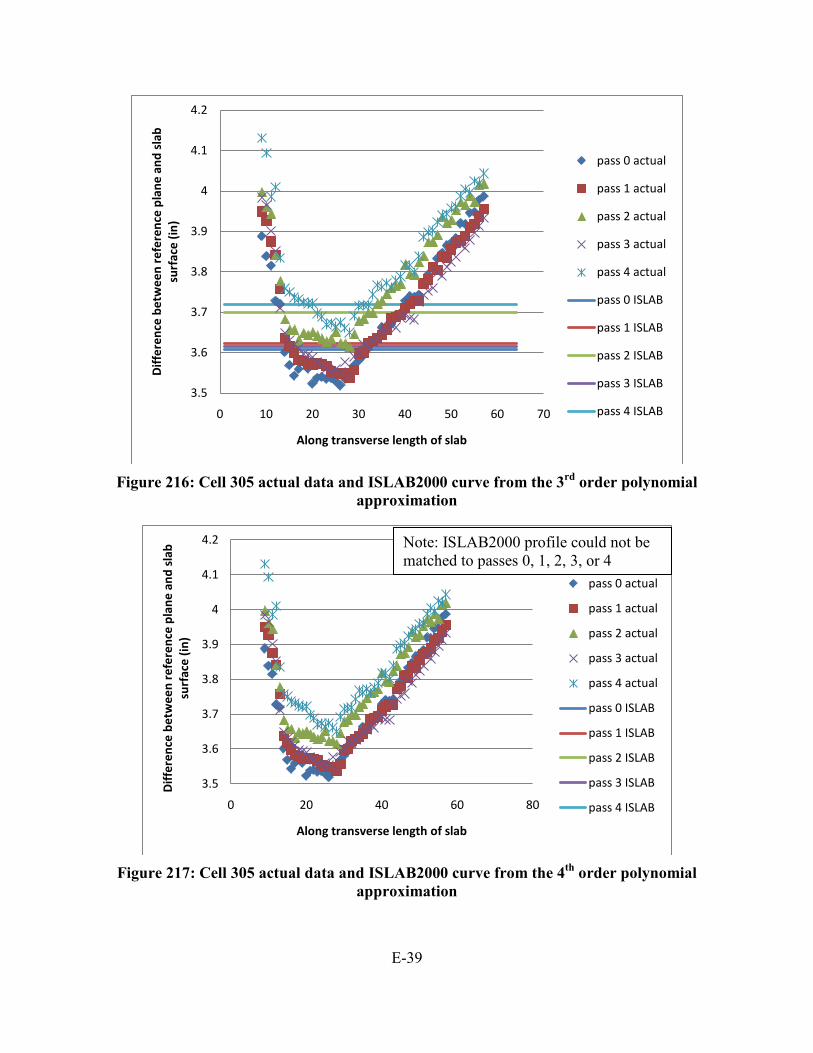
E-39
Figure 216: Cell 305 actual data and ISLAB2000 curve from the 3rd order polynomial
approximation
Figure 217: Cell 305 actual data and ISLAB2000 curve from the 4th order polynomial
approximation
3.5
3.6
3.7
3.8
3.9
4
4.1
4.2
0 10 20 30 40 50 60 70
Diff
eren
ce b
etw
een
refe
renc
e pl
ane
and
slab
su
rfac
e (in
)
Along transverse length of slab
pass 0 actual
pass 1 actual
pass 2 actual
pass 3 actual
pass 4 actual
pass 0 ISLAB
pass 1 ISLAB
pass 2 ISLAB
pass 3 ISLAB
pass 4 ISLAB
3.5
3.6
3.7
3.8
3.9
4
4.1
4.2
0 20 40 60 80
Diff
eren
ce b
etw
een
refe
renc
e pl
ane
and
slab
su
rfac
e (in
)
Along transverse length of slab
pass 0 actual
pass 1 actual
pass 2 actual
pass 3 actual
pass 4 actual
pass 0 ISLAB
pass 1 ISLAB
pass 2 ISLAB
pass 3 ISLAB
pass 4 ISLAB
Note: ISLAB2000 profile could not be matched to passes 0, 1, 2, 3, or 4

E-40
Figure 218: Cell 305 actual data and ISLAB2000 curve from the 5th order polynomial
approximation
Figure 219: Cell 305 actual data and ISLAB2000 curve from the 6th order polynomial
approximation
3.5
3.6
3.7
3.8
3.9
4
4.1
4.2
0 10 20 30 40 50 60 70
Diff
eren
ce b
etw
een
refe
renc
e pl
ane
and
slab
su
rfac
e (in
)
Along transverse length of slab
pass 0 actual
pass 1 actual
pass 2 actual
pass 3 actual
pass 4 actual
pass 0 ISLAB
pass 1 ISLAB
pass 2 ISLAB
pass 3 ISLAB
pass 4 ISLAB
3.5
3.6
3.7
3.8
3.9
4
4.1
4.2
0 10 20 30 40 50 60 70
Diff
eren
tial
Def
lect
ion
betw
een
Slab
and
Dat
um
(in)
Along transverse length of slab
pass 0 actual
pass 1 actual
pass 2 actual
pass 3 actual
pass 4 actual
pass 0 ISLAB
pass 1 ISLAB
pass 2 ISLAB
pass 3 ISLAB
pass 4 ISLAB
Note: ISLAB2000 profile could not be matched to passes 0, 1, 2, 3, or 4
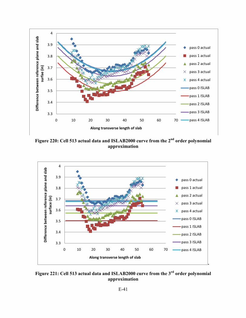
E-41
Figure 220: Cell 513 actual data and ISLAB2000 curve from the 2nd order polynomial
approximation
.
Figure 221: Cell 513 actual data and ISLAB2000 curve from the 3rd order polynomial approximation
3.3
3.4
3.5
3.6
3.7
3.8
3.9
4
0 10 20 30 40 50 60 70
Diff
eren
ce b
etw
een
refe
renc
e pl
ane
and
slab
su
rfae
(in)
Along transverse length of slab
pass 0 actual
pass 1 actual
pass 2 actual
pass 3 actual
pass 4 actual
pass 0 ISLAB
pass 1 ISLAB
pass 2 ISLAB
pass 3 ISLAB
pass 4 ISLAB
3.3
3.4
3.5
3.6
3.7
3.8
3.9
4
0 10 20 30 40 50 60 70
Diff
eren
ce b
etw
een
refe
renc
e pl
ane
and
slab
su
rfac
e (in
)
Along transverse length of slab
pass 0 actual
pass 1 actual
pass 2 actual
pass 3 actual
pass 4 actual
pass 0 ISLAB
pass 1 ISLAB
pass 2 ISLAB
pass 3 ISLAB
pass 4 ISLAB

E-42
Figure 222: Cell 513 actual data and ISLAB2000 curve from the 4th order polynomial
approximation
Figure 223: Cell 513 actual data and ISLAB2000 curve from the 5th order polynomial
approximation
3.3
3.4
3.5
3.6
3.7
3.8
3.9
4
0 10 20 30 40 50 60 70
Diff
eren
ce b
etw
een
refe
renc
e pl
ane
and
slab
su
rfac
e (in
)
Along transverse length of slab
pass 0 actual
pass 1 actual
pass 2 actual
pass 3 actual
pass 4 actual
pass 0 ISLAB
pass 1 ISLAB
pass 2 ISLAB
pass 3 ISLAB
pass 4 ISLAB
3.3
3.4
3.5
3.6
3.7
3.8
3.9
4
0 10 20 30 40 50 60 70
Diff
eren
ce b
etw
een
refe
renc
e pl
ane
and
slab
su
rfac
e (in
)
Along transverse length of slab
pass 0 actual
pass 1 actual
pass 2 actual
pass 3 actual
pass 4 actual
pass 0 ISLAB
pass 1 ISLAB
pass 2 ISLAB
pass 3 ISLAB
pass 4 ISLAB
Note: ISLAB2000 profile could not be matched to pass 4
Note: ISLAB2000 profile could not be matched to passes 0, 1, 2, 3, or 4
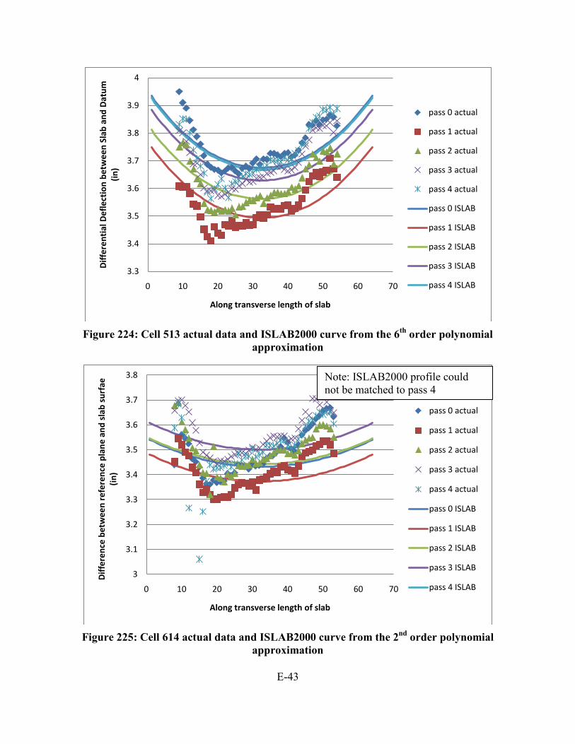
E-43
Figure 224: Cell 513 actual data and ISLAB2000 curve from the 6th order polynomial
approximation
Figure 225: Cell 614 actual data and ISLAB2000 curve from the 2nd order polynomial
approximation
3.3
3.4
3.5
3.6
3.7
3.8
3.9
4
0 10 20 30 40 50 60 70
Diff
eren
tial
Def
lect
ion
betw
een
Slab
and
Dat
um
(in)
Along transverse length of slab
pass 0 actual
pass 1 actual
pass 2 actual
pass 3 actual
pass 4 actual
pass 0 ISLAB
pass 1 ISLAB
pass 2 ISLAB
pass 3 ISLAB
pass 4 ISLAB
3
3.1
3.2
3.3
3.4
3.5
3.6
3.7
3.8
0 10 20 30 40 50 60 70
Diff
eren
ce b
etw
een
refe
renc
e pl
ane
and
slab
sur
fae
(in)
Along transverse length of slab
pass 0 actual
pass 1 actual
pass 2 actual
pass 3 actual
pass 4 actual
pass 0 ISLAB
pass 1 ISLAB
pass 2 ISLAB
pass 3 ISLAB
pass 4 ISLAB
Note: ISLAB2000 profile could not be matched to pass 4
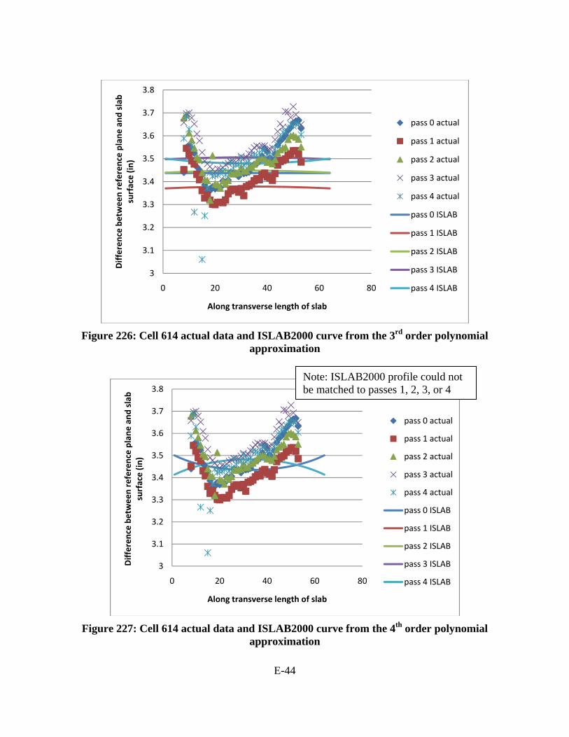
E-44
Figure 226: Cell 614 actual data and ISLAB2000 curve from the 3rd order polynomial approximation
Figure 227: Cell 614 actual data and ISLAB2000 curve from the 4th order polynomial approximation
3
3.1
3.2
3.3
3.4
3.5
3.6
3.7
3.8
0 20 40 60 80
Difference betw
een reference plane and slab
surface (in)
Along transverse length of slab
pass 0 actual
pass 1 actual
pass 2 actual
pass 3 actual
pass 4 actual
pass 0 ISLAB
pass 1 ISLAB
pass 2 ISLAB
pass 3 ISLAB
pass 4 ISLAB
3
3.1
3.2
3.3
3.4
3.5
3.6
3.7
3.8
0 20 40 60 80
Difference betw
een reference plane and slab
surface (in)
Along transverse length of slab
pass 0 actual
pass 1 actual
pass 2 actual
pass 3 actual
pass 4 actual
pass 0 ISLAB
pass 1 ISLAB
pass 2 ISLAB
pass 3 ISLAB
pass 4 ISLAB
Note: ISLAB2000 profile could not be matched to passes 1, 2, 3, or 4

E-45
Figure 228: Cell 614 actual data and ISLAB2000 curve from the 5th order polynomial
approximation
Figure 229: Cell 614 actual data and ISLAB2000 curve from the 6th order polynomial
approximation
3
3.1
3.2
3.3
3.4
3.5
3.6
3.7
3.8
3.9
0 20 40 60 80
Diff
eren
ce b
etw
een
refe
renc
e pl
ane
and
slab
su
rfac
e (in
)
Along transverse length of slab
pass 0 actual
pass 1 actual
pass 2 actual
pass 3 actual
pass 4 actual
pass 0 ISLAB
pass 1 ISLAB
pass 2 ISLAB
pass 3 ISLAB
pass 4 ISLAB
3
3.1
3.2
3.3
3.4
3.5
3.6
3.7
3.8
0 20 40 60 80
Diff
eren
tial
Def
lect
ion
betw
een
Slab
and
D
atum
(in)
Along transverse length of slab
pass 0 actual
pass 1 actual
pass 2 actual
pass 3 actual
pass 4 actual
pass 0 ISLAB
pass 1 ISLAB
pass 2 ISLAB
pass 3 ISLAB
pass 4 ISLAB
Note: ISLAB2000 profile could not be matched to passes 0 or 4

APPENDIX F: POLYNOMIAL APPROXIMATIONS OF ACTUAL DATA AND ASSOCIATED ISLAB CURVES
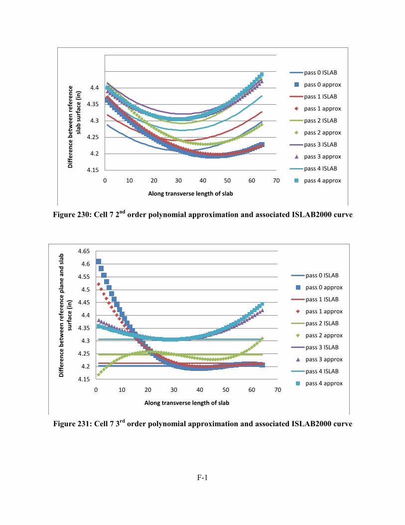
F-1
4.45
4.5
pla
ne a
nd
Figure 230: Cell 7 2nd order polynomial approximation and associated ISLAB2000 curve
Figure 231: Cell 7 3rd order polynomial approximation and associated ISLAB2000 curve
4.15
4.2
4.25
4.3
4.35
4.4
0 10 20 30 40 50 60 70
Diff
eren
ce b
etw
een
refe
renc
esl
ab s
urfa
ce (i
n)
Along transverse length of slab
pass 0 ISLAB
pass 0 approx
pass 1 ISLAB
pass 1 approx
pass 2 ISLAB
pass 2 approx
pass 3 ISLAB
pass 3 approx
pass 4 ISLAB
pass 4 approx
4.15
4.2
4.25
4.3
4.35
4.4
4.45
4.5
4.55
4.6
4.65
0 10 20 30 40 50 60 70
Diff
eren
ce b
etw
een
refe
renc
e pl
ane
and
slab
su
rfac
e (in
)
Along transverse length of slab
pass 0 ISLAB
pass 0 approx
pass 1 ISLAB
pass 1 approx
pass 2 ISLAB
pass 2 approx
pass 3 ISLAB
pass 3 approx
pass 4 ISLAB
pass 4 approx
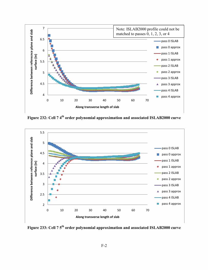
F-2
Figure 232: Cell 7 4th order polynomial approximation and associated ISLAB2000 curve
Figure 233: Cell 7 5th order polynomial approximation and associated ISLAB2000 curve
4
4.5
5
5.5
6
6.5
7
0 10 20 30 40 50 60 70
Diff
eren
ce b
etw
een
refe
recn
ce p
lane
and
sla
b su
rfac
e (in
)
Along transverse length of slab
pass 0 ISLAB
pass 0 approx
pass 1 ISLAB
pass 1 approx
pass 2 ISLAB
pass 2 approx
pass 3 ISLAB
pass 3 approx
pass 4 ISLAB
pass 4 approx
2
2.5
3
3.5
4
4.5
5
5.5
0 10 20 30 40 50 60 70
Diff
eren
ce b
etw
een
refe
renc
e pl
ane
and
slab
su
rfac
e (in
)
Along transverse length of slab
pass 0 ISLAB
pass 0 approx
pass 1 ISLAB
pass 1 approx
pass 2 ISLAB
pass 2 approx
pass 3 ISLAB
pass 3 approx
pass 4 ISLAB
pass 4 approx
Note: ISLAB2000 profile could not be matched to passes 0, 1, 2, 3, or 4
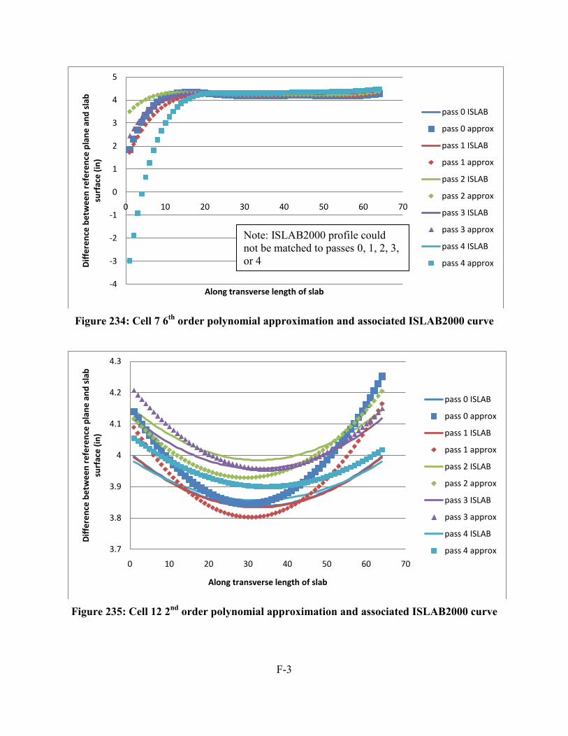
F-3
Figure 234: Cell 7 6th order polynomial approximation and associated ISLAB2000 curve
Figure 235: Cell 12 2nd order polynomial approximation and associated ISLAB2000 curve
-4
-3
-2
-1
0
1
2
3
4
5
0 10 20 30 40 50 60 70
Diff
eren
ce b
etw
een
refe
renc
e pl
ane
and
slab
su
rfac
e (in
)
Along transverse length of slab
pass 0 ISLAB
pass 0 approx
pass 1 ISLAB
pass 1 approx
pass 2 ISLAB
pass 2 approx
pass 3 ISLAB
pass 3 approx
pass 4 ISLAB
pass 4 approx
3.7
3.8
3.9
4
4.1
4.2
4.3
0 10 20 30 40 50 60 70
Diff
eren
ce b
etw
een
refe
renc
e pl
ane
and
slab
su
rfac
e (in
)
Along transverse length of slab
pass 0 ISLAB
pass 0 approx
pass 1 ISLAB
pass 1 approx
pass 2 ISLAB
pass 2 approx
pass 3 ISLAB
pass 3 approx
pass 4 ISLAB
pass 4 approx
Note: ISLAB2000 profile could not be matched to passes 0, 1, 2, 3, or 4

F-4
Figure 236: Cell 12 3rd order polynomial approximation and associated ISLAB2000 curve
Figure 237: Cell 12 4th order polynomial approximation and associated ISLAB2000 curve
3.7
3.8
3.9
4
4.1
4.2
4.3
4.4
4.5
0 10 20 30 40 50 60 70
Diff
eren
ce b
etw
een
refe
renc
e pl
ane
and
slab
su
rfac
e (in
)
Along transverse length of slab
pass 0 ISLAB
pass 0 approx
pass 1 ISLAB
pass 1 approx
pass 2 ISLAB
pass 2 approx
pass 3 ISLAB
pass 3 approx
pass 4 ISLAB
pass 4 approx
3.4
3.5
3.6
3.7
3.8
3.9
4
4.1
4.2
0 10 20 30 40 50 60 70
Diff
eren
ce b
etw
een
refe
recn
ce p
lane
and
sla
b su
rfac
e (in
)
Along transverse length of slab
pass 0 ISLAB
pass 0 approx
pass 1 ISLAB
pass 1 approx
pass 2 ISLAB
pass 2 approx
pass 3 ISLAB
pass 3 approx
pass 4 ISLAB
pass 4 approx
Note: ISLAB2000 profile could not be matched to passes 2, 3, or 4
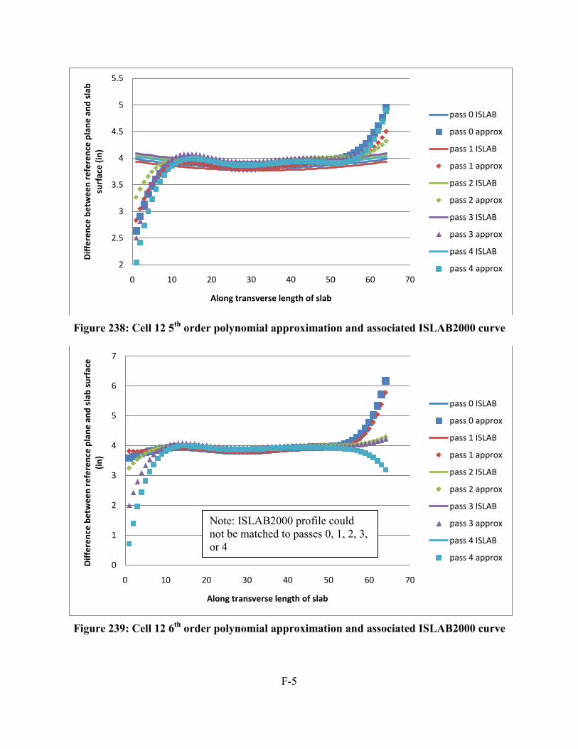
F-5
Figure 238: Cell 12 5th order polynomial approximation and associated ISLAB2000 curve
Figure 239: Cell 12 6th order polynomial approximation and associated ISLAB2000 curve
2
2.5
3
3.5
4
4.5
5
5.5
0 10 20 30 40 50 60 70
Diff
eren
ce b
etw
een
refe
renc
e pl
ane
and
slab
su
rfac
e (in
)
Along transverse length of slab
pass 0 ISLAB
pass 0 approx
pass 1 ISLAB
pass 1 approx
pass 2 ISLAB
pass 2 approx
pass 3 ISLAB
pass 3 approx
pass 4 ISLAB
pass 4 approx
0
1
2
3
4
5
6
7
0 10 20 30 40 50 60 70
Diff
eren
ce b
etw
een
refe
renc
e pl
ane
and
slab
sur
face
(in
)
Along transverse length of slab
pass 0 ISLAB
pass 0 approx
pass 1 ISLAB
pass 1 approx
pass 2 ISLAB
pass 2 approx
pass 3 ISLAB
pass 3 approx
pass 4 ISLAB
pass 4 approx
Note: ISLAB2000 profile could not be matched to passes 0, 1, 2, 3, or 4

F-6
Figure 240: Cell 36 panel 19 early morning 2nd order polynomial approximation and
associated ISLAB2000 curve
Figure 241: Cell 36 panel 19 early morning 3rd order polynomial approximation and
associated ISLAB2000 curve
3.5
3.6
3.7
3.8
3.9
4
4.1
4.2
0 10 20 30 40 50 60 70
Diff
eren
ce b
etw
een
refe
renc
e pl
ane
and
slab
su
rfac
e (in
)
Along transverse length of slab
pass 0 ISLAB
pass 0 approx
pass 1 ISLAB
pass 1 approx
pass 2 ISLAB
pass 2 approx
pass 3 ISLAB
pass 3 approx
pass 4 ISLAB
pass 4 approx
3.4
3.5
3.6
3.7
3.8
3.9
4
0 10 20 30 40 50 60 70
Diff
eren
ce b
etw
een
refe
renc
e pl
ane
and
slab
su
rfac
e (in
)
Along transverse length of slab
pass 0 ISLAB
pass 0 approx
pass 1 ISLAB
pass 1 approx
pass 2 ISLAB
pass 2 approx
pass 3 ISLAB
pass 3 approx
pass 4 ISLAB
pass 4 approx
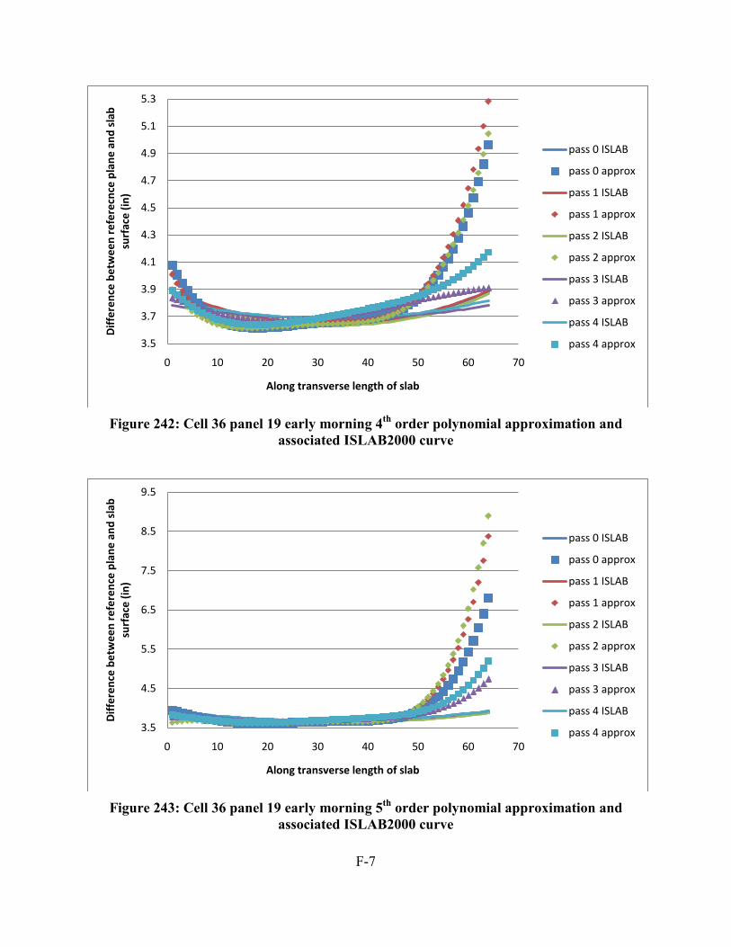
F-7
Figure 242: Cell 36 panel 19 early morning 4th order polynomial approximation and
associated ISLAB2000 curve
Figure 243: Cell 36 panel 19 early morning 5th order polynomial approximation and
associated ISLAB2000 curve
3.5
3.7
3.9
4.1
4.3
4.5
4.7
4.9
5.1
5.3
0 10 20 30 40 50 60 70
Diff
eren
ce b
etw
een
refe
recn
ce p
lane
and
sla
b su
rfac
e (in
)
Along transverse length of slab
pass 0 ISLAB
pass 0 approx
pass 1 ISLAB
pass 1 approx
pass 2 ISLAB
pass 2 approx
pass 3 ISLAB
pass 3 approx
pass 4 ISLAB
pass 4 approx
3.5
4.5
5.5
6.5
7.5
8.5
9.5
0 10 20 30 40 50 60 70
Diff
eren
ce b
etw
een
refe
renc
e pl
ane
and
slab
su
rfac
e (in
)
Along transverse length of slab
pass 0 ISLAB
pass 0 approx
pass 1 ISLAB
pass 1 approx
pass 2 ISLAB
pass 2 approx
pass 3 ISLAB
pass 3 approx
pass 4 ISLAB
pass 4 approx

F-8
Figure 244: Cell 36 panel 19 early morning 6th order polynomial approximation and
associated ISLAB2000 curve
Figure 245: Cell 36 panel 19 late morning 2nd order polynomial approximation and
associated ISLAB2000 curve
3
5
7
9
11
13
15
17
19
21
23
0 10 20 30 40 50 60 70
Diff
eren
ce b
etw
een
refe
renc
e pl
ane
and
slab
su
rfac
e (in
)
Along transverse length of slab
pass 0 ISLAB
pass 0 approx
pass 1 ISLAB
pass 1 approx
pass 2 ISLAB
pass 2 approx
pass 3 ISLAB
pass 3 approx
pass 4 ISLAB
pass 4 approx
3.9
4
4.1
4.2
4.3
4.4
4.5
0 10 20 30 40 50 60 70
Diff
eren
ce b
etw
een
refe
renc
e pl
ane
and
slab
su
rfac
e (in
)
Along transverse length of slab
pass 0 ISLAB
pass 0 approx
pass 1 ISLAB
pass 1 approx
pass 2 ISLAB
pass 2 approx
pass 3 ISLAB
pass 3 approx
pass 4 ISLAB
pass 4 approx

F-9
Figure 246: Cell 36 panel 19 late morning 3rd order polynomial approximation and
associated ISLAB2000 curve
Figure 247: Cell 36 panel 19 late morning 4th order polynomial approximation and
associated ISLAB2000 curve
3.8
4
4.2
4.4
4.6
4.8
5
5.2
5.4
5.6
5.8
0 10 20 30 40 50 60 70
Diff
eren
ce b
etw
een
refe
renc
e pl
ane
and
slab
su
rfac
e (in
)
Along transverse length of slab
pass 0 ISLAB
pass 0 approx
pass 1 ISLAB
pass 1 approx
pass 2 ISLAB
pass 2 approx
pass 3 ISLAB
pass 3 approx
pass 4 ISLAB
pass 4 approx
3.8
4.3
4.8
5.3
5.8
6.3
6.8
7.3
7.8
8.3
0 10 20 30 40 50 60 70
Diff
eren
ce b
etw
een
refe
recn
ce p
lane
and
sla
b su
rfac
e (in
)
Along transverse length of slab
pass 0 ISLAB
pass 0 approx
pass 1 ISLAB
pass 1 approx
pass 2 ISLAB
pass 2 approx
pass 3 ISLAB
pass 3 approx
pass 4 ISLAB
pass 4 approx

F-10
Figure 248: Cell 36 panel 19 late morning 5th order polynomial approximation and
associated ISLAB2000 curve
Figure 249: Cell 36 panel 19 late morning 6th order polynomial approximation and
associated ISLAB2000 curve
-10
-8
-6
-4
-2
0
2
4
6
8
0 10 20 30 40 50 60 70
Diff
eren
ce b
etw
een
refe
renc
e pl
ane
and
slab
su
rfac
e (in
)
Along transverse length of slab
pass 0 ISLAB
pass 0 approx
pass 1 ISLAB
pass 1 approx
pass 2 ISLAB
pass 2 approx
pass 3 ISLAB
pass 3 approx
pass 4 ISLAB
pass 4 approx
-10
-5
0
5
10
15
0 10 20 30 40 50 60 70
Diff
eren
ce b
etw
een
refe
renc
e pl
ane
and
slab
su
rfac
e (in
)
Along transverse length of slab
pass 0 ISLAB
pass 0 approx
pass 1 ISLAB
pass 1 approx
pass 2 ISLAB
pass 2 approx
pass 3 ISLAB
pass 3 approx
pass 4 ISLAB
pass 4 approx
Note: ISLAB2000 profile could not be matched to passes 0, 1, 2, 3, or 4
Note: ISLAB2000 profile could not be matched to passes 0, 1, 2, 3, or 4
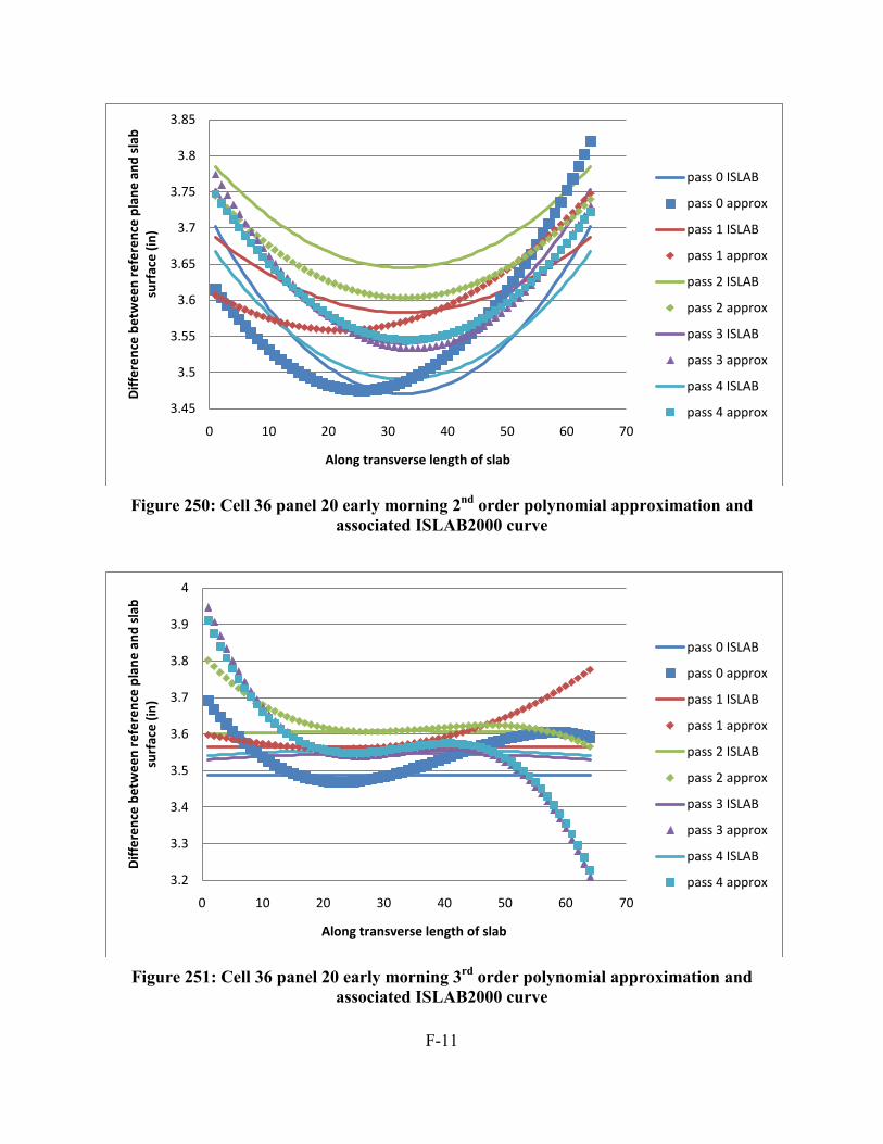
F-11
Figure 250: Cell 36 panel 20 early morning 2nd order polynomial approximation and
associated ISLAB2000 curve
Figure 251: Cell 36 panel 20 early morning 3rd order polynomial approximation and
associated ISLAB2000 curve
3.45
3.5
3.55
3.6
3.65
3.7
3.75
3.8
3.85
0 10 20 30 40 50 60 70
Diff
eren
ce b
etw
een
refe
renc
e pl
ane
and
slab
su
rfac
e (in
)
Along transverse length of slab
pass 0 ISLAB
pass 0 approx
pass 1 ISLAB
pass 1 approx
pass 2 ISLAB
pass 2 approx
pass 3 ISLAB
pass 3 approx
pass 4 ISLAB
pass 4 approx
3.2
3.3
3.4
3.5
3.6
3.7
3.8
3.9
4
0 10 20 30 40 50 60 70
Diff
eren
ce b
etw
een
refe
renc
e pl
ane
and
slab
su
rfac
e (in
)
Along transverse length of slab
pass 0 ISLAB
pass 0 approx
pass 1 ISLAB
pass 1 approx
pass 2 ISLAB
pass 2 approx
pass 3 ISLAB
pass 3 approx
pass 4 ISLAB
pass 4 approx
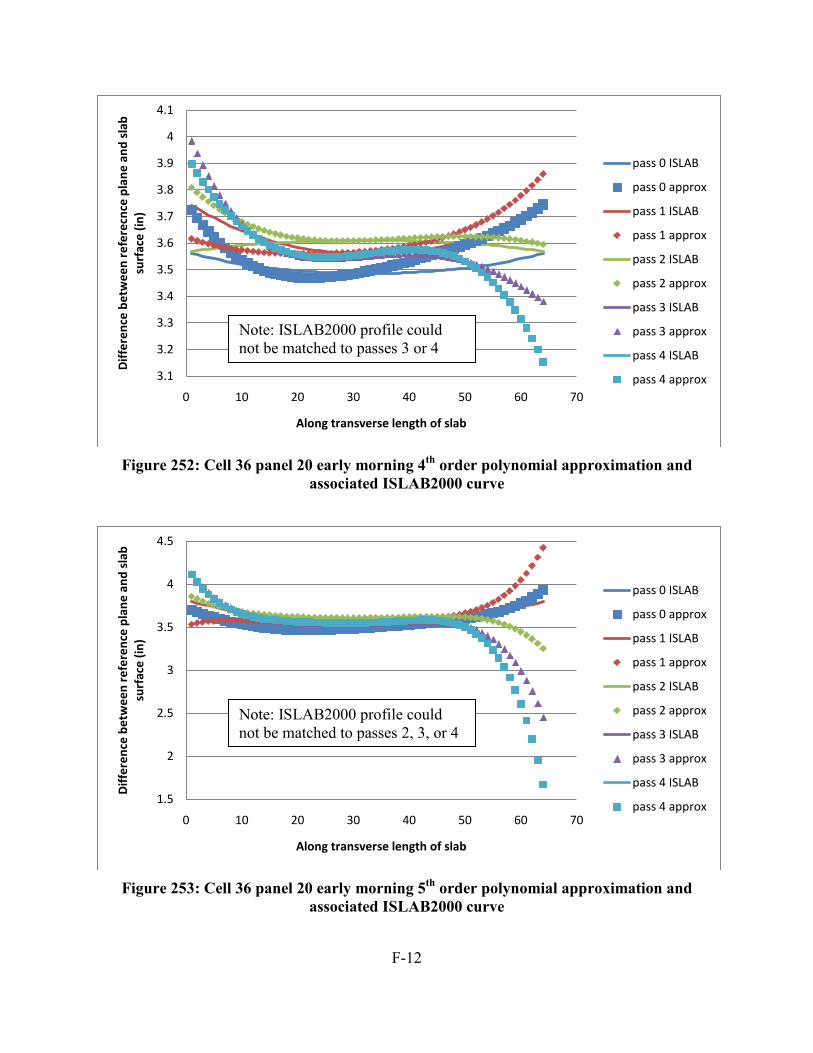
F-12
Figure 252: Cell 36 panel 20 early morning 4th order polynomial approximation and
associated ISLAB2000 curve
Figure 253: Cell 36 panel 20 early morning 5th order polynomial approximation and
associated ISLAB2000 curve
3.1
3.2
3.3
3.4
3.5
3.6
3.7
3.8
3.9
4
4.1
0 10 20 30 40 50 60 70
Diff
eren
ce b
etw
een
refe
recn
ce p
lane
and
sla
b su
rfac
e (in
)
Along transverse length of slab
pass 0 ISLAB
pass 0 approx
pass 1 ISLAB
pass 1 approx
pass 2 ISLAB
pass 2 approx
pass 3 ISLAB
pass 3 approx
pass 4 ISLAB
pass 4 approx
1.5
2
2.5
3
3.5
4
4.5
0 10 20 30 40 50 60 70
Diff
eren
ce b
etw
een
refe
renc
e pl
ane
and
slab
su
rfac
e (in
)
Along transverse length of slab
pass 0 ISLAB
pass 0 approx
pass 1 ISLAB
pass 1 approx
pass 2 ISLAB
pass 2 approx
pass 3 ISLAB
pass 3 approx
pass 4 ISLAB
pass 4 approx
Note: ISLAB2000 profile could not be matched to passes 3 or 4
Note: ISLAB2000 profile could not be matched to passes 2, 3, or 4
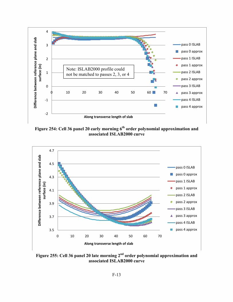
F-13
Figure 254: Cell 36 panel 20 early morning 6th order polynomial approximation and
associated ISLAB2000 curve
Figure 255: Cell 36 panel 20 late morning 2nd order polynomial approximation and
associated ISLAB2000 curve
-2
-1
0
1
2
3
4
0 10 20 30 40 50 60 70
Diff
eren
ce b
etw
een
refe
renc
e pl
ane
and
slab
su
rfac
e (in
)
Along transverse length of slab
pass 0 ISLAB
pass 0 approx
pass 1 ISLAB
pass 1 approx
pass 2 ISLAB
pass 2 approx
pass 3 ISLAB
pass 3 approx
pass 4 ISLAB
pass 4 approx
3.5
3.7
3.9
4.1
4.3
4.5
4.7
0 10 20 30 40 50 60 70
Diff
eren
ce b
etw
een
refe
renc
e pl
ane
and
slab
su
rfac
e (in
)
Along transverse length of slab
pass 0 ISLAB
pass 0 approx
pass 1 ISLAB
pass 1 approx
pass 2 ISLAB
pass 2 approx
pass 3 ISLAB
pass 3 approx
pass 4 ISLAB
pass 4 approx
Note: ISLAB2000 profile could not be matched to passes 2, 3, or 4

F-14
Figure 256: Cell 36 panel 20 late morning 3rd order polynomial approximation and
associated ISLAB2000 curve
Figure 257: Cell 36 panel 20 late morning 4th order polynomial approximation and
associated ISLAB2000 curve
3.5
3.7
3.9
4.1
4.3
4.5
4.7
4.9
5.1
5.3
0 10 20 30 40 50 60 70
Diff
eren
ce b
etw
een
refe
renc
e pl
ane
and
slab
su
rfac
e (in
)
Along transverse length of slab
pass 0 ISLAB
pass 0 approx
pass 1 ISLAB
pass 1 approx
pass 2 ISLAB
pass 2 approx
pass 3 ISLAB
pass 3 approx
pass 4 ISLAB
pass 4 approx
3.5
3.7
3.9
4.1
4.3
4.5
4.7
4.9
5.1
5.3
5.5
0 10 20 30 40 50 60 70
Diff
eren
ce b
etw
een
refe
recn
ce p
lane
and
sla
b su
rfac
e (in
)
Along transverse length of slab
pass 0 ISLAB
pass 0 approx
pass 1 ISLAB
pass 1 approx
pass 2 ISLAB
pass 2 approx
pass 3 ISLAB
pass 3 approx
pass 4 ISLAB
pass 4 approx
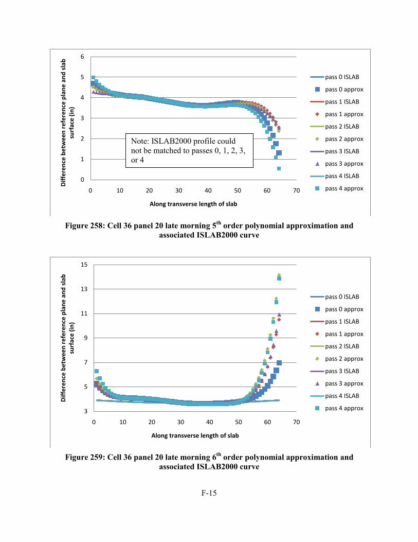
F-15
Figure 258: Cell 36 panel 20 late morning 5th order polynomial approximation and
associated ISLAB2000 curve
Figure 259: Cell 36 panel 20 late morning 6th order polynomial approximation and
associated ISLAB2000 curve
0
1
2
3
4
5
6
0 10 20 30 40 50 60 70
Diff
eren
ce b
etw
een
refe
renc
e pl
ane
and
slab
su
rfac
e (in
)
Along transverse length of slab
pass 0 ISLAB
pass 0 approx
pass 1 ISLAB
pass 1 approx
pass 2 ISLAB
pass 2 approx
pass 3 ISLAB
pass 3 approx
pass 4 ISLAB
pass 4 approx
3
5
7
9
11
13
15
0 10 20 30 40 50 60 70
Diff
eren
ce b
etw
een
refe
renc
e pl
ane
and
slab
su
rfac
e (in
)
Along transverse length of slab
pass 0 ISLAB
pass 0 approx
pass 1 ISLAB
pass 1 approx
pass 2 ISLAB
pass 2 approx
pass 3 ISLAB
pass 3 approx
pass 4 ISLAB
pass 4 approx
Note: ISLAB2000 profile could not be matched to passes 0, 1, 2, 3, or 4
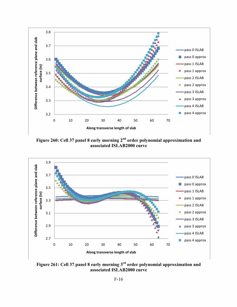
F-16
Figure 260: Cell 37 panel 8 early morning 2nd order polynomial approximation and
associated ISLAB2000 curve
Figure 261: Cell 37 panel 8 early morning 3rd order polynomial approximation and
associated ISLAB2000 curve
3.2
3.3
3.4
3.5
3.6
3.7
3.8
0 10 20 30 40 50 60 70
Diff
eren
ce b
etw
een
refe
renc
e pl
ane
and
slab
su
rfac
e (in
)
Along transverse length of slab
pass 0 ISLAB
pass 0 approx
pass 1 ISLAB
pass 1 approx
pass 2 ISLAB
pass 2 approx
pass 3 ISLAB
pass 3 approx
pass 4 ISLAB
pass 4 approx
2.7
2.9
3.1
3.3
3.5
3.7
3.9
0 10 20 30 40 50 60 70
Diff
eren
ce b
etw
een
refe
renc
e pl
ane
and
slab
su
rfac
e (in
)
Along transverse length of slab
pass 0 ISLAB
pass 0 approx
pass 1 ISLAB
pass 1 approx
pass 2 ISLAB
pass 2 approx
pass 3 ISLAB
pass 3 approx
pass 4 ISLAB
pass 4 approx
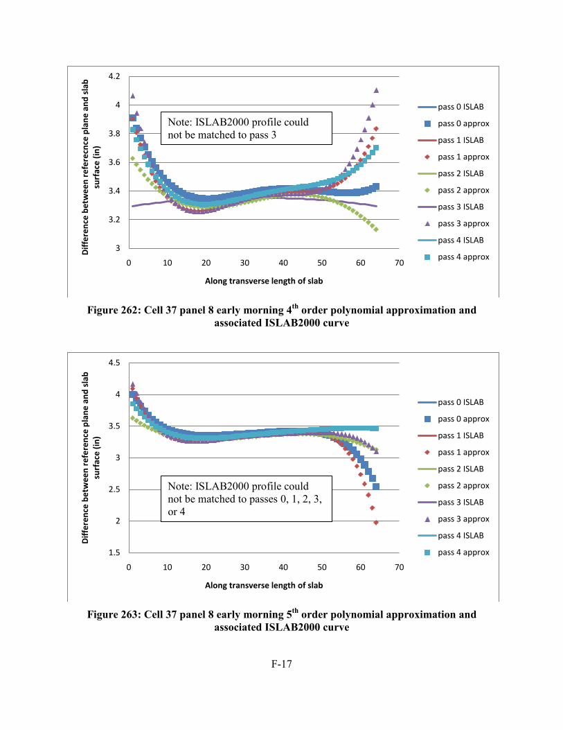
F-17
Figure 262: Cell 37 panel 8 early morning 4th order polynomial approximation and
associated ISLAB2000 curve
Figure 263: Cell 37 panel 8 early morning 5th order polynomial approximation and
associated ISLAB2000 curve
3
3.2
3.4
3.6
3.8
4
4.2
0 10 20 30 40 50 60 70
Diff
eren
ce b
etw
een
refe
recn
ce p
lane
and
sla
b su
rfac
e (in
)
Along transverse length of slab
pass 0 ISLAB
pass 0 approx
pass 1 ISLAB
pass 1 approx
pass 2 ISLAB
pass 2 approx
pass 3 ISLAB
pass 3 approx
pass 4 ISLAB
pass 4 approx
1.5
2
2.5
3
3.5
4
4.5
0 10 20 30 40 50 60 70
Diff
eren
ce b
etw
een
refe
renc
e pl
ane
and
slab
su
rfac
e (in
)
Along transverse length of slab
pass 0 ISLAB
pass 0 approx
pass 1 ISLAB
pass 1 approx
pass 2 ISLAB
pass 2 approx
pass 3 ISLAB
pass 3 approx
pass 4 ISLAB
pass 4 approx
Note: ISLAB2000 profile could not be matched to pass 3
Note: ISLAB2000 profile could not be matched to passes 0, 1, 2, 3, or 4
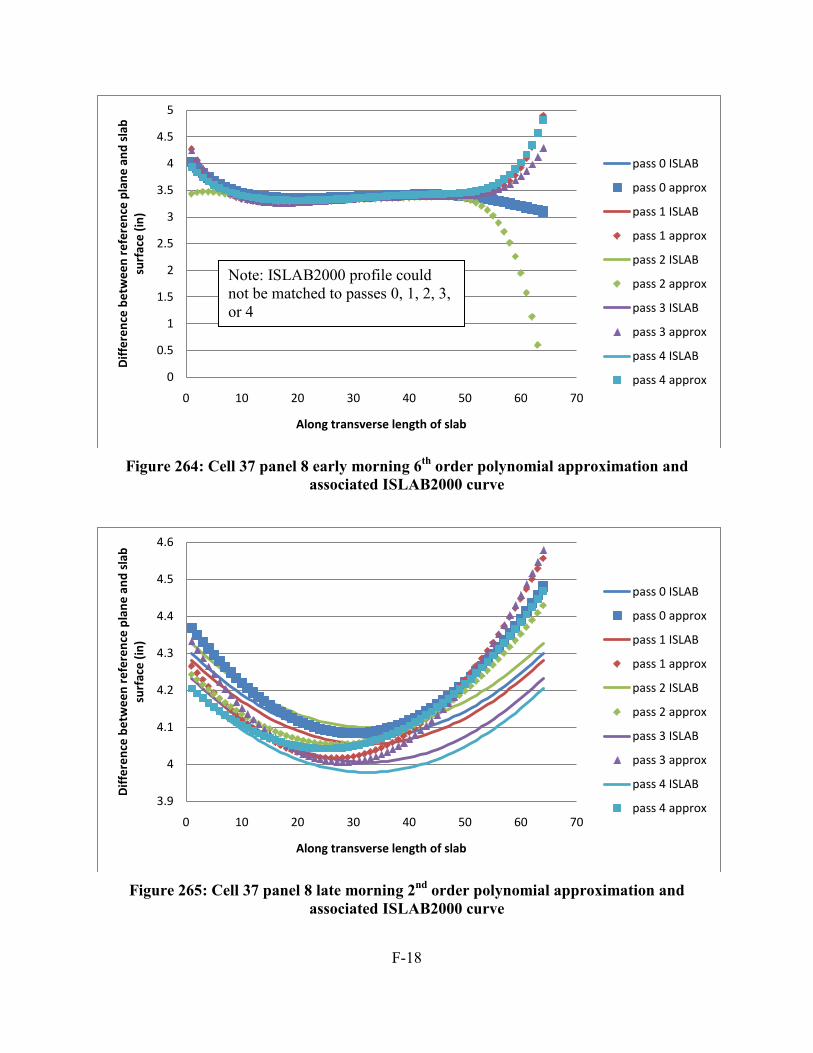
F-18
Figure 264: Cell 37 panel 8 early morning 6th order polynomial approximation and
associated ISLAB2000 curve
Figure 265: Cell 37 panel 8 late morning 2nd order polynomial approximation and
associated ISLAB2000 curve
0
0.5
1
1.5
2
2.5
3
3.5
4
4.5
5
0 10 20 30 40 50 60 70
Diff
eren
ce b
etw
een
refe
renc
e pl
ane
and
slab
su
rfac
e (in
)
Along transverse length of slab
pass 0 ISLAB
pass 0 approx
pass 1 ISLAB
pass 1 approx
pass 2 ISLAB
pass 2 approx
pass 3 ISLAB
pass 3 approx
pass 4 ISLAB
pass 4 approx
3.9
4
4.1
4.2
4.3
4.4
4.5
4.6
0 10 20 30 40 50 60 70
Diff
eren
ce b
etw
een
refe
renc
e pl
ane
and
slab
su
rfac
e (in
)
Along transverse length of slab
pass 0 ISLAB
pass 0 approx
pass 1 ISLAB
pass 1 approx
pass 2 ISLAB
pass 2 approx
pass 3 ISLAB
pass 3 approx
pass 4 ISLAB
pass 4 approx
Note: ISLAB2000 profile could not be matched to passes 0, 1, 2, 3, or 4
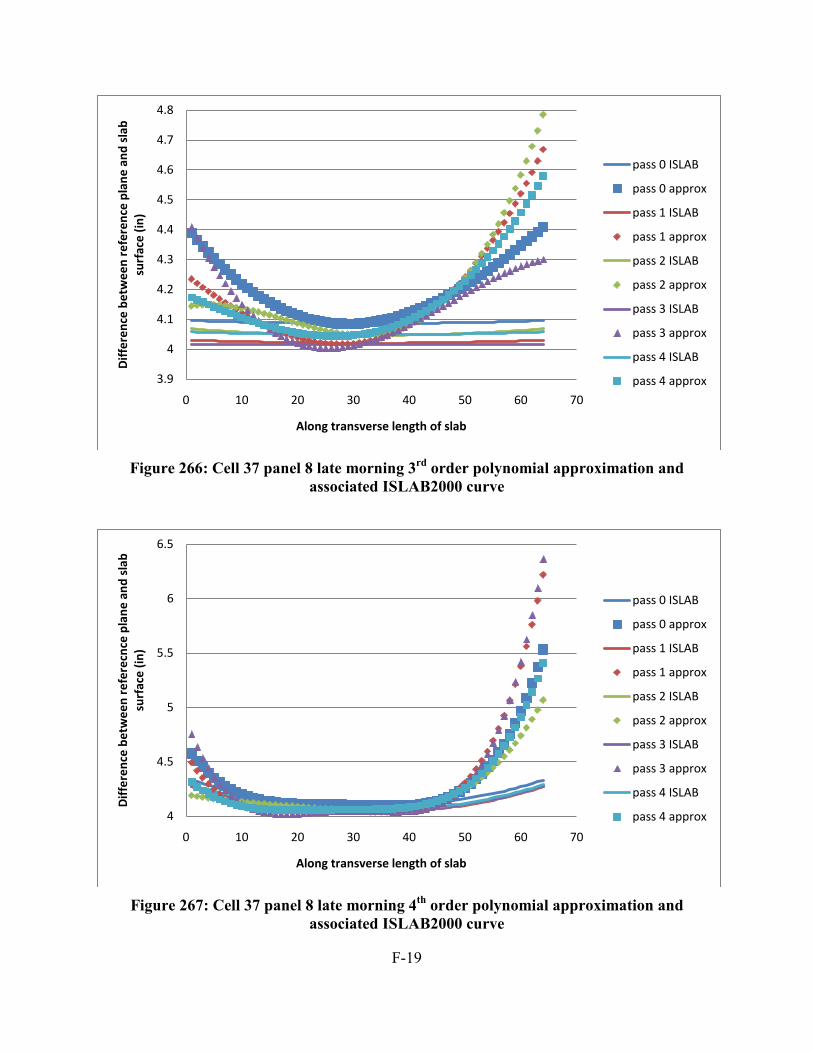
F-19
Figure 266: Cell 37 panel 8 late morning 3rd order polynomial approximation and
associated ISLAB2000 curve
Figure 267: Cell 37 panel 8 late morning 4th order polynomial approximation and
associated ISLAB2000 curve
3.9
4
4.1
4.2
4.3
4.4
4.5
4.6
4.7
4.8
0 10 20 30 40 50 60 70
Diff
eren
ce b
etw
een
refe
renc
e pl
ane
and
slab
su
rfac
e (in
)
Along transverse length of slab
pass 0 ISLAB
pass 0 approx
pass 1 ISLAB
pass 1 approx
pass 2 ISLAB
pass 2 approx
pass 3 ISLAB
pass 3 approx
pass 4 ISLAB
pass 4 approx
4
4.5
5
5.5
6
6.5
0 10 20 30 40 50 60 70
Diff
eren
ce b
etw
een
refe
recn
ce p
lane
and
sla
b su
rfac
e (in
)
Along transverse length of slab
pass 0 ISLAB
pass 0 approx
pass 1 ISLAB
pass 1 approx
pass 2 ISLAB
pass 2 approx
pass 3 ISLAB
pass 3 approx
pass 4 ISLAB
pass 4 approx
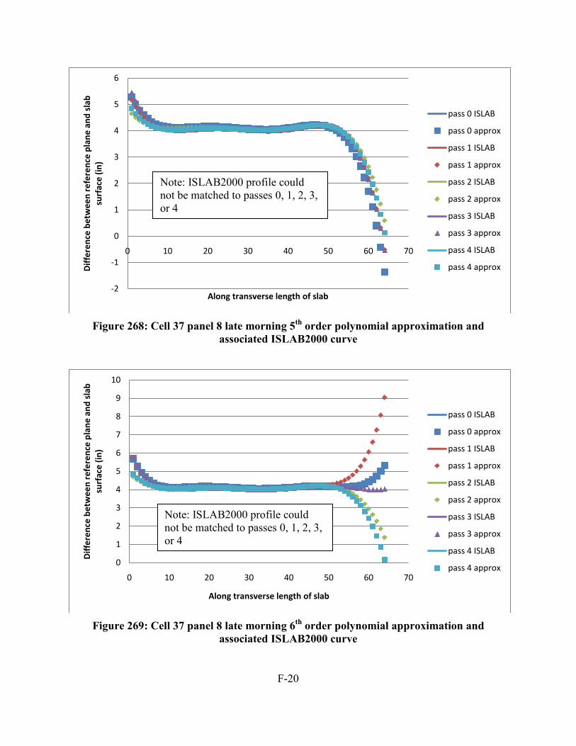
F-20
Figure 268: Cell 37 panel 8 late morning 5th order polynomial approximation and
associated ISLAB2000 curve
Figure 269: Cell 37 panel 8 late morning 6th order polynomial approximation and
associated ISLAB2000 curve
-2
-1
0
1
2
3
4
5
6
0 10 20 30 40 50 60 70
Diff
eren
ce b
etw
een
refe
renc
e pl
ane
and
slab
su
rfac
e (in
)
Along transverse length of slab
pass 0 ISLAB
pass 0 approx
pass 1 ISLAB
pass 1 approx
pass 2 ISLAB
pass 2 approx
pass 3 ISLAB
pass 3 approx
pass 4 ISLAB
pass 4 approx
0
1
2
3
4
5
6
7
8
9
10
0 10 20 30 40 50 60 70
Diff
eren
ce b
etw
een
refe
renc
e pl
ane
and
slab
su
rfac
e (in
)
Along transverse length of slab
pass 0 ISLAB
pass 0 approx
pass 1 ISLAB
pass 1 approx
pass 2 ISLAB
pass 2 approx
pass 3 ISLAB
pass 3 approx
pass 4 ISLAB
pass 4 approx
Note: ISLAB2000 profile could not be matched to passes 0, 1, 2, 3, or 4
Note: ISLAB2000 profile could not be matched to passes 0, 1, 2, 3, or 4
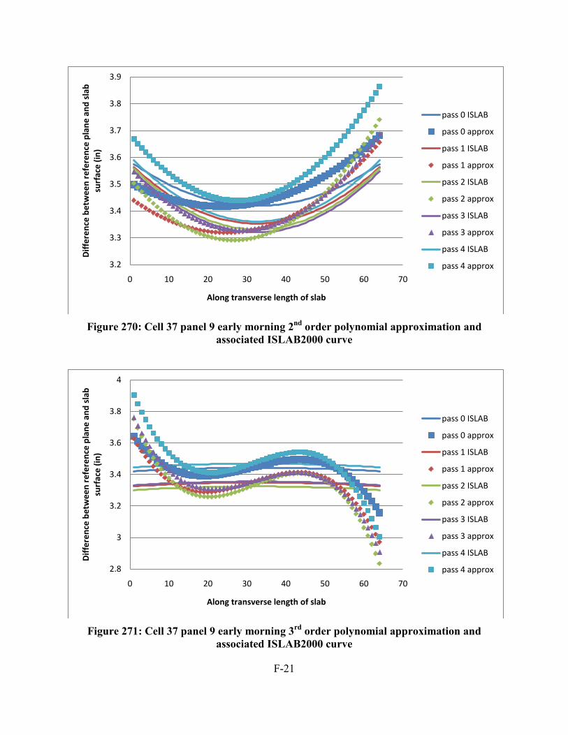
F-21
Figure 270: Cell 37 panel 9 early morning 2nd order polynomial approximation and
associated ISLAB2000 curve
Figure 271: Cell 37 panel 9 early morning 3rd order polynomial approximation and
associated ISLAB2000 curve
3.2
3.3
3.4
3.5
3.6
3.7
3.8
3.9
0 10 20 30 40 50 60 70
Diff
eren
ce b
etw
een
refe
renc
e pl
ane
and
slab
su
rfac
e (in
)
Along transverse length of slab
pass 0 ISLAB
pass 0 approx
pass 1 ISLAB
pass 1 approx
pass 2 ISLAB
pass 2 approx
pass 3 ISLAB
pass 3 approx
pass 4 ISLAB
pass 4 approx
2.8
3
3.2
3.4
3.6
3.8
4
0 10 20 30 40 50 60 70
Diff
eren
ce b
etw
een
refe
renc
e pl
ane
and
slab
su
rfac
e (in
)
Along transverse length of slab
pass 0 ISLAB
pass 0 approx
pass 1 ISLAB
pass 1 approx
pass 2 ISLAB
pass 2 approx
pass 3 ISLAB
pass 3 approx
pass 4 ISLAB
pass 4 approx

F-22
Figure 272: Cell 37 panel 9 early morning 4th order polynomial approximation and
associated ISLAB2000 curve
Figure 273: Cell 37 panel 9 early morning 5th order polynomial approximation and
associated ISLAB2000 curve
3.2
3.3
3.4
3.5
3.6
3.7
3.8
3.9
4
4.1
4.2
0 10 20 30 40 50 60 70
Diff
eren
ce b
etw
een
refe
recn
ce p
lane
and
sla
b su
rfac
e (in
)
Along transverse length of slab
pass 0 ISLAB
pass 0 approx
pass 1 ISLAB
pass 1 approx
pass 2 ISLAB
pass 2 approx
pass 3 ISLAB
pass 3 approx
pass 4 ISLAB
pass 4 approx
0
0.5
1
1.5
2
2.5
3
3.5
4
4.5
0 10 20 30 40 50 60 70
Diff
eren
ce b
etw
een
refe
renc
e pl
ane
and
slab
su
rfac
e (in
)
Along transverse length of slab
pass 0 ISLAB
pass 0 approx
pass 1 ISLAB
pass 1 approx
pass 2 ISLAB
pass 2 approx
pass 3 ISLAB
pass 3 approx
pass 4 ISLAB
pass 4 approx
Note: ISLAB2000 profile could not be matched to passes 1, 2, 3, or 4
Note: ISLAB2000 profile could not be matched to passes 0, 1, 2, 3, or 4

F-23
Figure 274: Cell 37 panel 9 early morning 6th order polynomial approximation and
associated ISLAB2000 curve
Figure 275: Cell 37 panel 9 late morning 2nd order polynomial approximation and
associated ISLAB2000 curve
2.5
3
3.5
4
4.5
5
5.5
6
6.5
7
0 10 20 30 40 50 60 70
Diff
eren
ce b
etw
een
refe
renc
e pl
ane
and
slab
su
rfac
e (in
)
Along transverse length of slab
pass 0 ISLAB
pass 0 approx
pass 1 ISLAB
pass 1 approx
pass 2 ISLAB
pass 2 approx
pass 3 ISLAB
pass 3 approx
pass 4 ISLAB
pass 4 approx
4
4.1
4.2
4.3
4.4
4.5
4.6
0 10 20 30 40 50 60 70
Diff
eren
ce b
etw
een
refe
renc
e pl
ane
and
slab
sur
face
(in
)
Along transverse length of slab
pass 0 ISLAB
pass 0 approx
pass 1 ISLAB
pass 1 approx
pass 2 ISLAB
pass 2 approx
pass 3 ISLAB
pass 3 approx
pass 4 ISLAB
pass 4 approx
Note: ISLAB2000 profile could not be matched to passes 0, 1, 2, 3, or 4
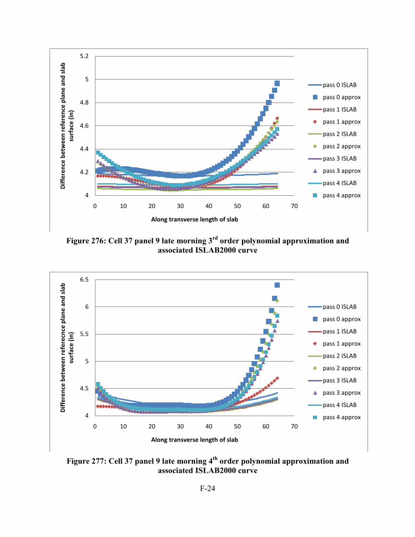
F-24
Figure 276: Cell 37 panel 9 late morning 3rd order polynomial approximation and
associated ISLAB2000 curve
Figure 277: Cell 37 panel 9 late morning 4th order polynomial approximation and
associated ISLAB2000 curve
4
4.2
4.4
4.6
4.8
5
5.2
0 10 20 30 40 50 60 70
Diff
eren
ce b
etw
een
refe
renc
e pl
ane
and
slab
su
rfac
e (in
)
Along transverse length of slab
pass 0 ISLAB
pass 0 approx
pass 1 ISLAB
pass 1 approx
pass 2 ISLAB
pass 2 approx
pass 3 ISLAB
pass 3 approx
pass 4 ISLAB
pass 4 approx
4
4.5
5
5.5
6
6.5
0 10 20 30 40 50 60 70
Diff
eren
ce b
etw
een
refe
recn
ce p
lane
and
sla
b su
rfac
e (in
)
Along transverse length of slab
pass 0 ISLAB
pass 0 approx
pass 1 ISLAB
pass 1 approx
pass 2 ISLAB
pass 2 approx
pass 3 ISLAB
pass 3 approx
pass 4 ISLAB
pass 4 approx
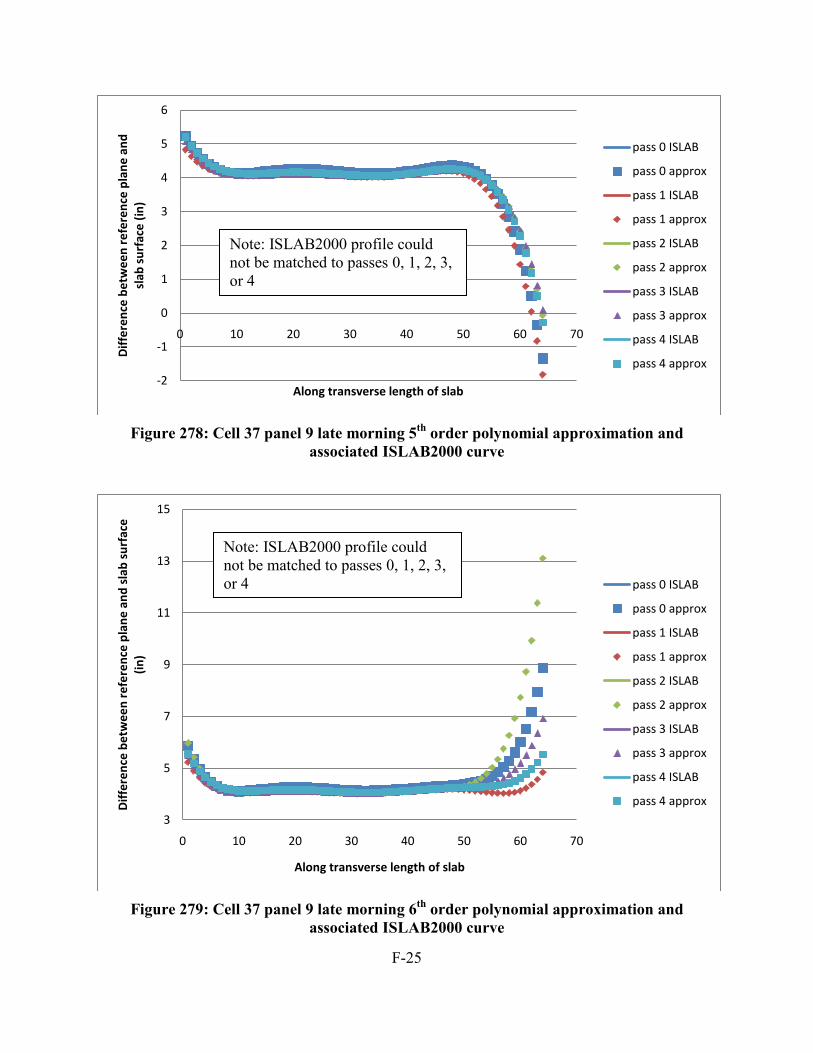
F-25
Figure 278: Cell 37 panel 9 late morning 5th order polynomial approximation and
associated ISLAB2000 curve
Figure 279: Cell 37 panel 9 late morning 6th order polynomial approximation and
associated ISLAB2000 curve
-2
-1
0
1
2
3
4
5
6
0 10 20 30 40 50 60 70
Diff
eren
ce b
etw
een
refe
renc
e pl
ane
and
slab
sur
face
(in)
Along transverse length of slab
pass 0 ISLAB
pass 0 approx
pass 1 ISLAB
pass 1 approx
pass 2 ISLAB
pass 2 approx
pass 3 ISLAB
pass 3 approx
pass 4 ISLAB
pass 4 approx
3
5
7
9
11
13
15
0 10 20 30 40 50 60 70
Diff
eren
ce b
etw
een
refe
renc
e pl
ane
and
slab
sur
face
(in
)
Along transverse length of slab
pass 0 ISLAB
pass 0 approx
pass 1 ISLAB
pass 1 approx
pass 2 ISLAB
pass 2 approx
pass 3 ISLAB
pass 3 approx
pass 4 ISLAB
pass 4 approx
Note: ISLAB2000 profile could not be matched to passes 0, 1, 2, 3, or 4
Note: ISLAB2000 profile could not be matched to passes 0, 1, 2, 3, or 4
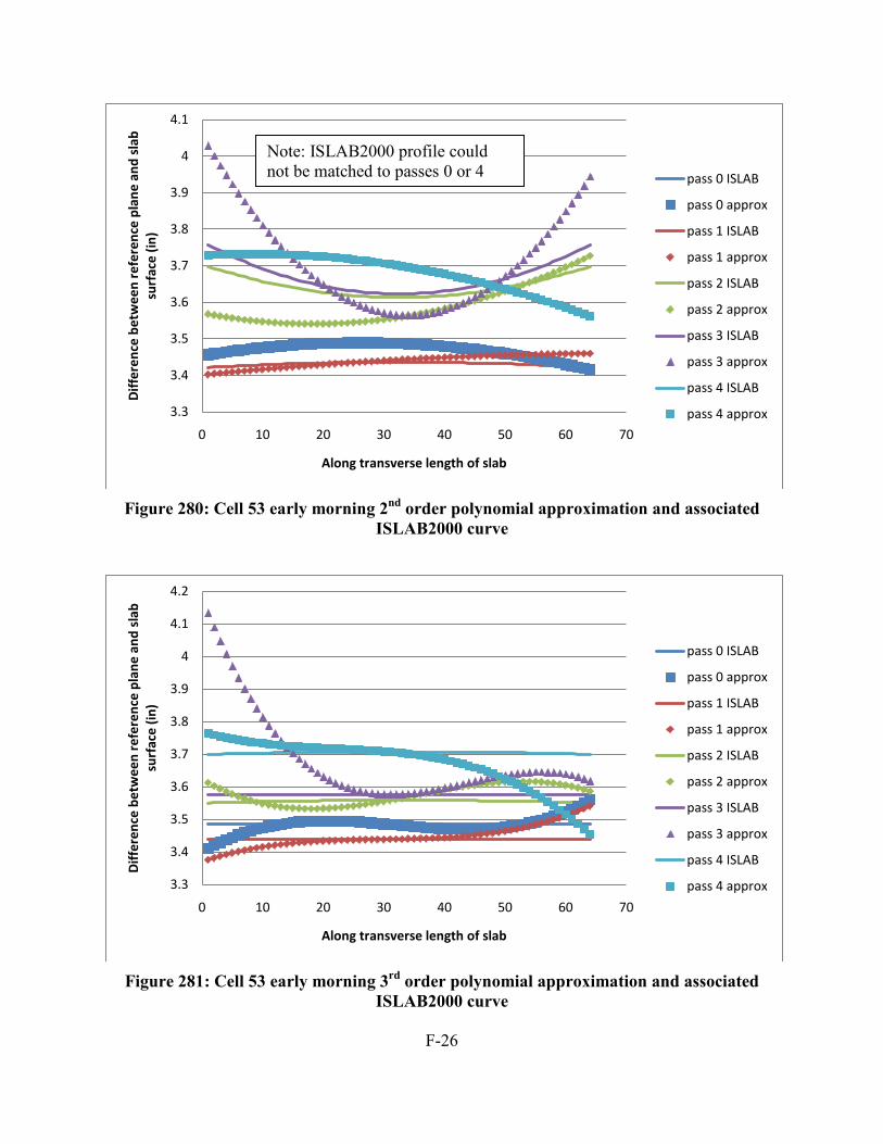
F-26
Figure 280: Cell 53 early morning 2nd order polynomial approximation and associated
ISLAB2000 curve
Figure 281: Cell 53 early morning 3rd order polynomial approximation and associated
ISLAB2000 curve
3.3
3.4
3.5
3.6
3.7
3.8
3.9
4
4.1
0 10 20 30 40 50 60 70
Diff
eren
ce b
etw
een
refe
renc
e pl
ane
and
slab
su
rfac
e (in
)
Along transverse length of slab
pass 0 ISLAB
pass 0 approx
pass 1 ISLAB
pass 1 approx
pass 2 ISLAB
pass 2 approx
pass 3 ISLAB
pass 3 approx
pass 4 ISLAB
pass 4 approx
3.3
3.4
3.5
3.6
3.7
3.8
3.9
4
4.1
4.2
0 10 20 30 40 50 60 70
Diff
eren
ce b
etw
een
refe
renc
e pl
ane
and
slab
su
rfac
e (in
)
Along transverse length of slab
pass 0 ISLAB
pass 0 approx
pass 1 ISLAB
pass 1 approx
pass 2 ISLAB
pass 2 approx
pass 3 ISLAB
pass 3 approx
pass 4 ISLAB
pass 4 approx
Note: ISLAB2000 profile could not be matched to passes 0 or 4
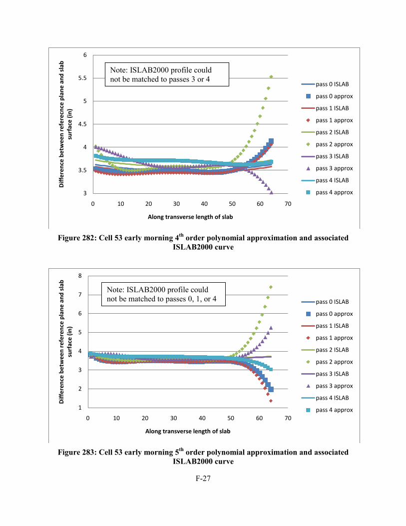
F-27
Figure 282: Cell 53 early morning 4th order polynomial approximation and associated
ISLAB2000 curve
Figure 283: Cell 53 early morning 5th order polynomial approximation and associated
ISLAB2000 curve
3
3.5
4
4.5
5
5.5
6
0 10 20 30 40 50 60 70
Diff
eren
ce b
etw
een
refe
recn
ce p
lane
and
sla
b su
rfac
e (in
)
Along transverse length of slab
pass 0 ISLAB
pass 0 approx
pass 1 ISLAB
pass 1 approx
pass 2 ISLAB
pass 2 approx
pass 3 ISLAB
pass 3 approx
pass 4 ISLAB
pass 4 approx
1
2
3
4
5
6
7
8
0 10 20 30 40 50 60 70
Diff
eren
ce b
etw
een
refe
renc
e pl
ane
and
slab
su
rfac
e (in
)
Along transverse length of slab
pass 0 ISLAB
pass 0 approx
pass 1 ISLAB
pass 1 approx
pass 2 ISLAB
pass 2 approx
pass 3 ISLAB
pass 3 approx
pass 4 ISLAB
pass 4 approx
Note: ISLAB2000 profile could not be matched to passes 3 or 4
Note: ISLAB2000 profile could not be matched to passes 0, 1, or 4

F-28
Figure 284: Cell 53 early morning 6th order polynomial approximation and associated
ISLAB2000 curve
Figure 285: Cell 53 late morning 2nd order polynomial approximation and associated
ISLAB2000 curve
2.5
3.5
4.5
5.5
6.5
7.5
8.5
0 10 20 30 40 50 60 70
Diff
eren
ce b
etw
een
refe
renc
e pl
ane
and
slab
su
rfac
e (in
)
Along transverse length of slab
pass 0 ISLAB
pass 0 approx
pass 1 ISLAB
pass 1 approx
pass 2 ISLAB
pass 2 approx
pass 3 ISLAB
pass 3 approx
pass 4 ISLAB
pass 4 approx
4.1
4.2
4.3
4.4
4.5
4.6
4.7
4.8
4.9
0 10 20 30 40 50 60 70
Diff
eren
ce b
etw
een
refe
renc
e pl
ane
and
slab
su
rfac
e (in
)
Along transverse length of slab
pass 0 ISLAB
pass 0 approx
pass 1 ISLAB
pass 1 approx
pass 2 ISLAB
pass 2 approx
pass 3 ISLAB
pass 3 approx
pass 4 ISLAB
pass 4 approx
Note: ISLAB2000 profile could not be matched to passes 0, 1, or 4
Note: ISLAB2000 profile could not be matched to passes 0 or 4
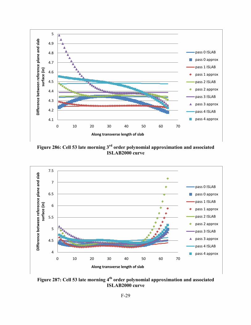
F-29
Figure 286: Cell 53 late morning 3rd order polynomial approximation and associated
ISLAB2000 curve
Figure 287: Cell 53 late morning 4th order polynomial approximation and associated
ISLAB2000 curve
4.1
4.2
4.3
4.4
4.5
4.6
4.7
4.8
4.9
5
0 10 20 30 40 50 60 70
Diff
eren
ce b
etw
een
refe
renc
e pl
ane
and
slab
su
rfac
e (in
)
Along transverse length of slab
pass 0 ISLAB
pass 0 approx
pass 1 ISLAB
pass 1 approx
pass 2 ISLAB
pass 2 approx
pass 3 ISLAB
pass 3 approx
pass 4 ISLAB
pass 4 approx
4
4.5
5
5.5
6
6.5
7
7.5
0 10 20 30 40 50 60 70
Diff
eren
ce b
etw
een
refe
recn
ce p
lane
and
sla
b su
rfac
e (in
)
Along transverse length of slab
pass 0 ISLAB
pass 0 approx
pass 1 ISLAB
pass 1 approx
pass 2 ISLAB
pass 2 approx
pass 3 ISLAB
pass 3 approx
pass 4 ISLAB
pass 4 approx

F-30
Figure 288: Cell 53 late morning 5th order polynomial approximation and associated
ISLAB2000 curve
Figure 289: Cell 53 late morning 6th order polynomial approximation and associated
ISLAB2000 curve
3
4
5
6
7
8
9
10
0 10 20 30 40 50 60 70
Diff
eren
ce b
etw
een
refe
renc
e pl
ane
and
slab
su
rfac
e (in
)
Along transverse length of slab
pass 0 ISLAB
pass 0 approx
pass 1 ISLAB
pass 1 approx
pass 2 ISLAB
pass 2 approx
pass 3 ISLAB
pass 3 approx
pass 4 ISLAB
pass 4 approx
2
4
6
8
10
12
14
16
0 10 20 30 40 50 60 70
Diff
eren
ce b
etw
een
refe
renc
e pl
ane
and
slab
su
rfac
e (in
)
Along transverse length of slab
pass 0 ISLAB
pass 0 approx
pass 1 ISLAB
pass 1 approx
pass 2 ISLAB
pass 2 approx
pass 3 ISLAB
pass 3 approx
pass 4 ISLAB
pass 4 approx
Note: ISLAB2000 profile could not be matched to passes 0, 1, or 4
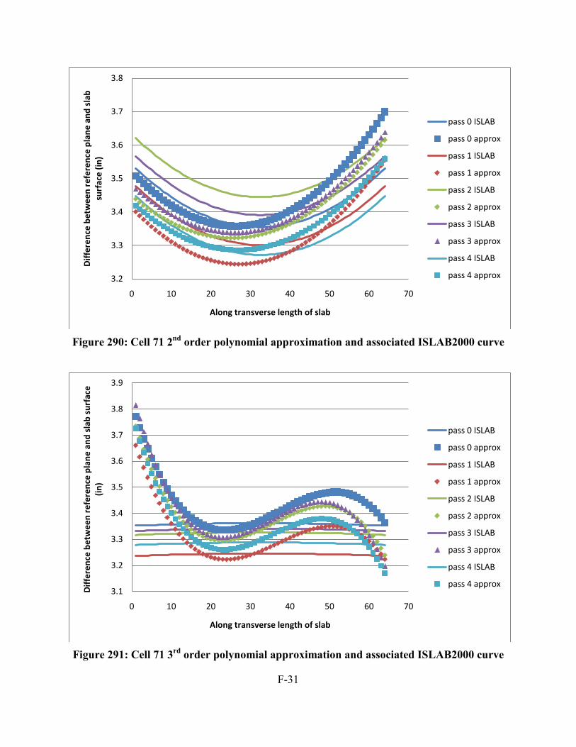
F-31
Figure 290: Cell 71 2nd order polynomial approximation and associated ISLAB2000 curve
Figure 291: Cell 71 3rd order polynomial approximation and associated ISLAB2000 curve
3.2
3.3
3.4
3.5
3.6
3.7
3.8
0 10 20 30 40 50 60 70
Diff
eren
ce b
etw
een
refe
renc
e pl
ane
and
slab
su
rfac
e (in
)
Along transverse length of slab
pass 0 ISLAB
pass 0 approx
pass 1 ISLAB
pass 1 approx
pass 2 ISLAB
pass 2 approx
pass 3 ISLAB
pass 3 approx
pass 4 ISLAB
pass 4 approx
3.1
3.2
3.3
3.4
3.5
3.6
3.7
3.8
3.9
0 10 20 30 40 50 60 70
Diff
eren
ce b
etw
een
refe
renc
e pl
ane
and
slab
sur
face
(in
)
Along transverse length of slab
pass 0 ISLAB
pass 0 approx
pass 1 ISLAB
pass 1 approx
pass 2 ISLAB
pass 2 approx
pass 3 ISLAB
pass 3 approx
pass 4 ISLAB
pass 4 approx
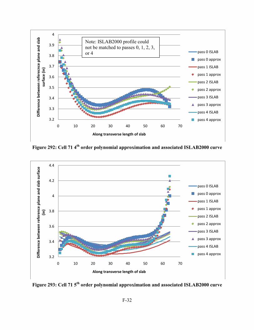
F-32
Figure 292: Cell 71 4th order polynomial approximation and associated ISLAB2000 curve
Figure 293: Cell 71 5th order polynomial approximation and associated ISLAB2000 curve
3.2
3.3
3.4
3.5
3.6
3.7
3.8
3.9
4
0 10 20 30 40 50 60 70
Diff
eren
ce b
etw
een
refe
recn
ce p
lane
and
sla
b su
rfac
e (in
)
Along transverse length of slab
pass 0 ISLAB
pass 0 approx
pass 1 ISLAB
pass 1 approx
pass 2 ISLAB
pass 2 approx
pass 3 ISLAB
pass 3 approx
pass 4 ISLAB
pass 4 approx
3.2
3.4
3.6
3.8
4
4.2
4.4
0 10 20 30 40 50 60 70
Diff
eren
ce b
etw
een
refe
renc
e pl
ane
and
slab
sur
face
(in
)
Along transverse length of slab
pass 0 ISLAB
pass 0 approx
pass 1 ISLAB
pass 1 approx
pass 2 ISLAB
pass 2 approx
pass 3 ISLAB
pass 3 approx
pass 4 ISLAB
pass 4 approx
Note: ISLAB2000 profile could not be matched to passes 0, 1, 2, 3, or 4
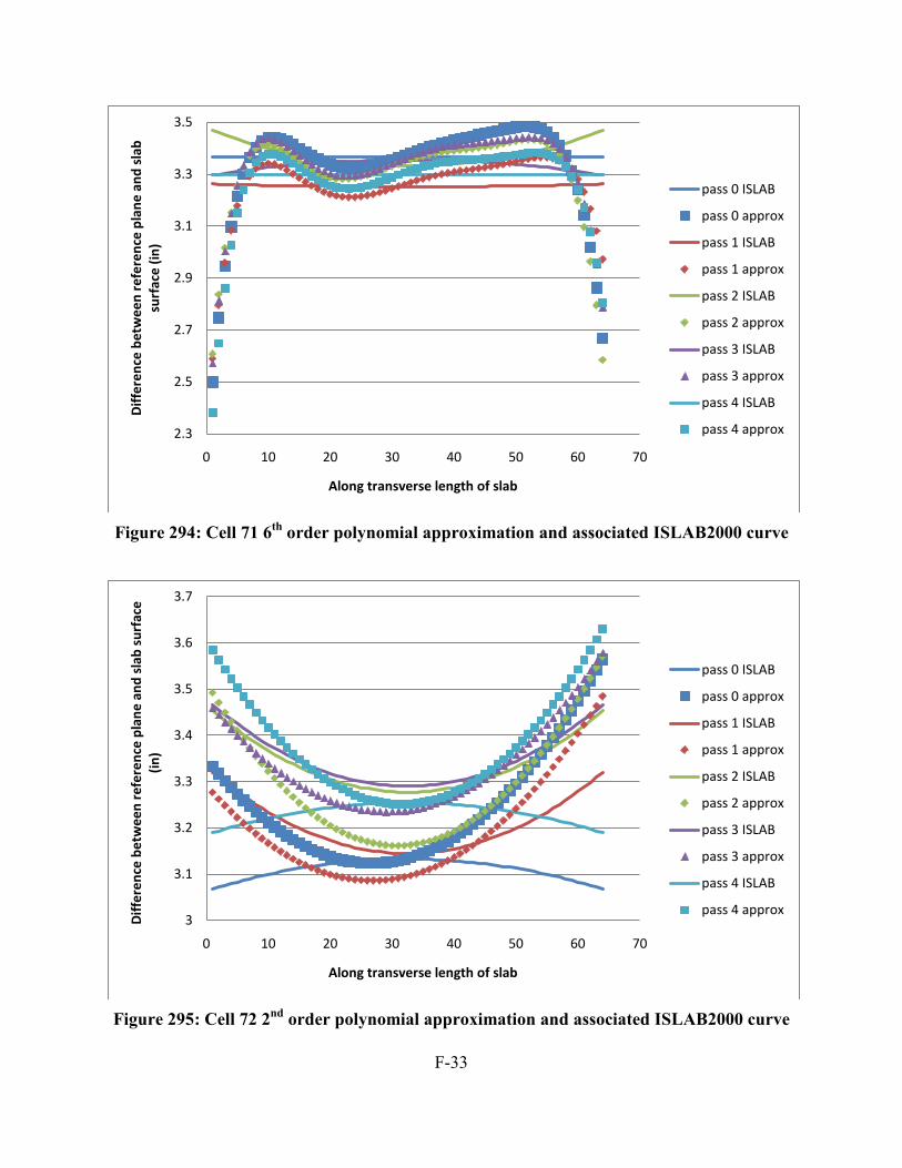
F-33
Figure 294: Cell 71 6th order polynomial approximation and associated ISLAB2000 curve
Figure 295: Cell 72 2nd order polynomial approximation and associated ISLAB2000 curve
2.3
2.5
2.7
2.9
3.1
3.3
3.5
0 10 20 30 40 50 60 70
Diff
eren
ce b
etw
een
refe
renc
e pl
ane
and
slab
su
rfac
e (in
)
Along transverse length of slab
pass 0 ISLAB
pass 0 approx
pass 1 ISLAB
pass 1 approx
pass 2 ISLAB
pass 2 approx
pass 3 ISLAB
pass 3 approx
pass 4 ISLAB
pass 4 approx
3
3.1
3.2
3.3
3.4
3.5
3.6
3.7
0 10 20 30 40 50 60 70
Diff
eren
ce b
etw
een
refe
renc
e pl
ane
and
slab
sur
face
(in
)
Along transverse length of slab
pass 0 ISLAB
pass 0 approx
pass 1 ISLAB
pass 1 approx
pass 2 ISLAB
pass 2 approx
pass 3 ISLAB
pass 3 approx
pass 4 ISLAB
pass 4 approx

F-34
Figure 296: Cell 72 3rd order polynomial approximation and associated ISLAB2000 curve
Figure 297: Cell 72 4th order polynomial approximation and associated ISLAB2000 curve
3
3.1
3.2
3.3
3.4
3.5
3.6
3.7
3.8
0 10 20 30 40 50 60 70
Diff
eren
ce b
etw
een
refe
renc
e pl
ane
and
slab
su
rfac
e (in
)
Along transverse length of slab
pass 0 ISLAB
pass 0 approx
pass 1 ISLAB
pass 1 approx
pass 2 ISLAB
pass 2 approx
pass 3 ISLAB
pass 3 approx
pass 4 ISLAB
pass 4 approx
3
3.1
3.2
3.3
3.4
3.5
3.6
3.7
3.8
3.9
4
0 10 20 30 40 50 60 70
Diff
eren
ce b
etw
een
refe
recn
ce p
lane
and
sla
b su
rfac
e (in
)
Along transverse length of slab
pass 0 ISLAB
pass 0 approx
pass 1 ISLAB
pass 1 approx
pass 2 ISLAB
pass 2 approx
pass 3 ISLAB
pass 3 approx
pass 4 ISLAB
pass 4 approx
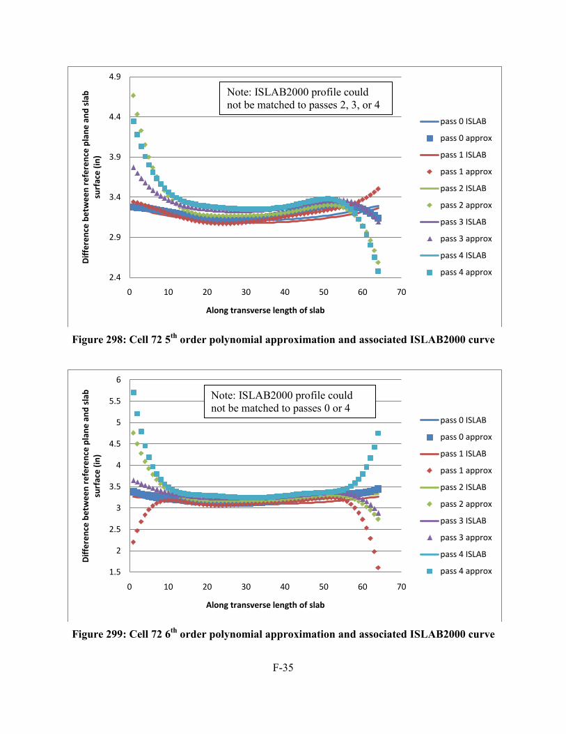
F-35
Figure 298: Cell 72 5th order polynomial approximation and associated ISLAB2000 curve
Figure 299: Cell 72 6th order polynomial approximation and associated ISLAB2000 curve
2.4
2.9
3.4
3.9
4.4
4.9
0 10 20 30 40 50 60 70
Diff
eren
ce b
etw
een
refe
renc
e pl
ane
and
slab
su
rfac
e (in
)
Along transverse length of slab
pass 0 ISLAB
pass 0 approx
pass 1 ISLAB
pass 1 approx
pass 2 ISLAB
pass 2 approx
pass 3 ISLAB
pass 3 approx
pass 4 ISLAB
pass 4 approx
1.5
2
2.5
3
3.5
4
4.5
5
5.5
6
0 10 20 30 40 50 60 70
Diff
eren
ce b
etw
een
refe
renc
e pl
ane
and
slab
su
rfac
e (in
)
Along transverse length of slab
pass 0 ISLAB
pass 0 approx
pass 1 ISLAB
pass 1 approx
pass 2 ISLAB
pass 2 approx
pass 3 ISLAB
pass 3 approx
pass 4 ISLAB
pass 4 approx
Note: ISLAB2000 profile could not be matched to passes 2, 3, or 4
Note: ISLAB2000 profile could not be matched to passes 0 or 4
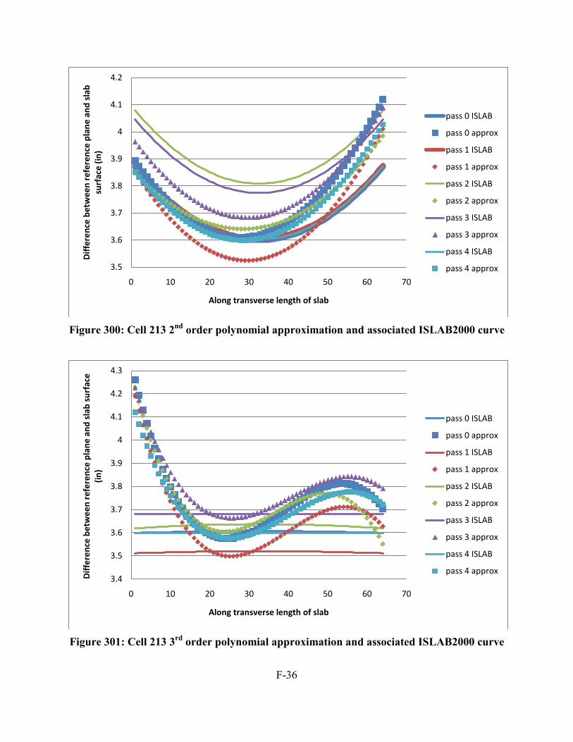
F-36
Figure 300: Cell 213 2nd order polynomial approximation and associated ISLAB2000 curve
Figure 301: Cell 213 3rd order polynomial approximation and associated ISLAB2000 curve
3.5
3.6
3.7
3.8
3.9
4
4.1
4.2
0 10 20 30 40 50 60 70
Diff
eren
ce b
etw
een
refe
renc
e pl
ane
and
slab
su
rfac
e (in
)
Along transverse length of slab
pass 0 ISLAB
pass 0 approx
pass 1 ISLAB
pass 1 approx
pass 2 ISLAB
pass 2 approx
pass 3 ISLAB
pass 3 approx
pass 4 ISLAB
pass 4 approx
3.4
3.5
3.6
3.7
3.8
3.9
4
4.1
4.2
4.3
0 10 20 30 40 50 60 70
Diff
eren
ce b
etw
een
refe
renc
e pl
ane
and
slab
sur
face
(in
)
Along transverse length of slab
pass 0 ISLAB
pass 0 approx
pass 1 ISLAB
pass 1 approx
pass 2 ISLAB
pass 2 approx
pass 3 ISLAB
pass 3 approx
pass 4 ISLAB
pass 4 approx
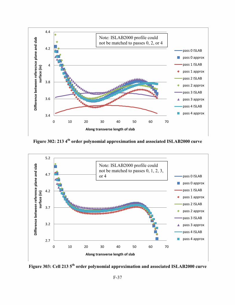
F-37
Figure 302: 213 4th order polynomial approximation and associated ISLAB2000 curve
Figure 303: Cell 213 5th order polynomial approximation and associated ISLAB2000 curve
3.4
3.6
3.8
4
4.2
4.4
0 10 20 30 40 50 60 70
Diff
eren
ce b
etw
een
refe
recn
ce p
lane
and
sla
b su
rfac
e (in
)
Along transverse length of slab
pass 0 ISLAB
pass 0 approx
pass 1 ISLAB
pass 1 approx
pass 2 ISLAB
pass 2 approx
pass 3 ISLAB
pass 3 approx
pass 4 ISLAB
pass 4 approx
2.7
3.2
3.7
4.2
4.7
5.2
0 10 20 30 40 50 60 70
Diff
eren
ce b
etw
een
refe
renc
e pl
ane
and
slab
su
rfac
e (in
)
Along transverse length of slab
pass 0 ISLAB
pass 0 approx
pass 1 ISLAB
pass 1 approx
pass 2 ISLAB
pass 2 approx
pass 3 ISLAB
pass 3 approx
pass 4 ISLAB
pass 4 approx
Note: ISLAB2000 profile could not be matched to passes 0, 2, or 4
Note: ISLAB2000 profile could not be matched to passes 0, 1, 2, 3, or 4

F-38
Figure 304: Cell 213 6th order polynomial approximation and associated ISLAB2000 curve
Figure 305: Cell 305 2nd order polynomial approximation and associated ISLAB2000 curve
-1
-0.5
0
0.5
1
1.5
2
2.5
3
3.5
4
0 10 20 30 40 50 60 70
Diff
eren
ce b
etw
een
refe
renc
e pl
ane
and
slab
sur
face
(in
)
Along transverse length of slab
pass 0 ISLAB
pass 0 approx
pass 1 ISLAB
pass 1 approx
pass 2 ISLAB
pass 2 approx
pass 3 ISLAB
pass 3 approx
pass 4 ISLAB
pass 4 approx
3.5
3.6
3.7
3.8
3.9
4
4.1
4.2
4.3
4.4
0 10 20 30 40 50 60 70
Diff
eren
ce b
etw
een
refe
renc
e pl
ane
and
slab
sur
face
(in
)
Along transverse length of slab
pass 0 ISLAB
pass 0 approx
pass 1 ISLAB
pass 1 approx
pass 2 ISLAB
pass 2 approx
pass 3 ISLAB
pass 3 approx
pass 4 ISLAB
pass 4 approx
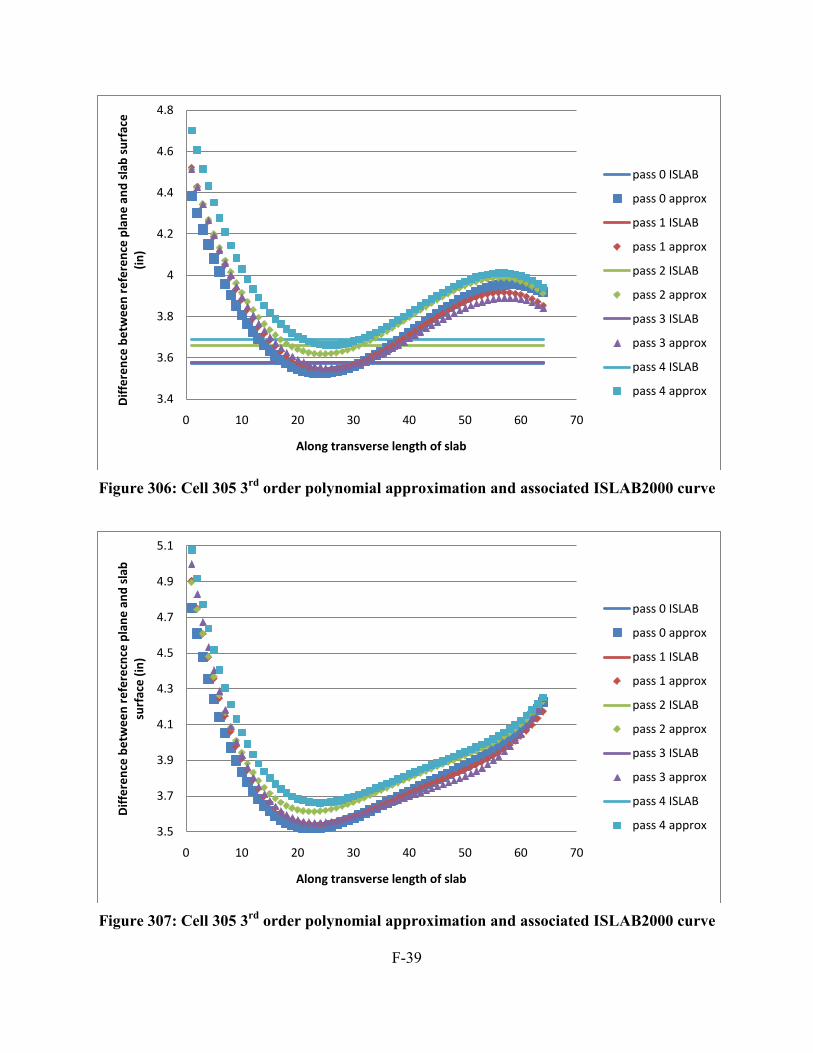
F-39
Figure 306: Cell 305 3rd order polynomial approximation and associated ISLAB2000 curve
Figure 307: Cell 305 3rd order polynomial approximation and associated ISLAB2000 curve
3.4
3.6
3.8
4
4.2
4.4
4.6
4.8
0 10 20 30 40 50 60 70
Diff
eren
ce b
etw
een
refe
renc
e pl
ane
and
slab
sur
face
(in
)
Along transverse length of slab
pass 0 ISLAB
pass 0 approx
pass 1 ISLAB
pass 1 approx
pass 2 ISLAB
pass 2 approx
pass 3 ISLAB
pass 3 approx
pass 4 ISLAB
pass 4 approx
3.5
3.7
3.9
4.1
4.3
4.5
4.7
4.9
5.1
0 10 20 30 40 50 60 70
Diff
eren
ce b
etw
een
refe
recn
ce p
lane
and
sla
b su
rfac
e (in
)
Along transverse length of slab
pass 0 ISLAB
pass 0 approx
pass 1 ISLAB
pass 1 approx
pass 2 ISLAB
pass 2 approx
pass 3 ISLAB
pass 3 approx
pass 4 ISLAB
pass 4 approx

F-40
Figure 308: Cell 305 4th order polynomial approximation and associated ISLAB2000 curve
Figure 309: Cell 305 5th order polynomial approximation and associated ISLAB2000 curve
3.5
3.7
3.9
4.1
4.3
4.5
4.7
4.9
5.1
0 10 20 30 40 50 60 70
Diff
eren
ce b
etw
een
refe
recn
ce p
lane
and
sla
b su
rfac
e (in
)
Along transverse length of slab
pass 0 ISLAB
pass 0 approx
pass 1 ISLAB
pass 1 approx
pass 2 ISLAB
pass 2 approx
pass 3 ISLAB
pass 3 approx
pass 4 ISLAB
pass 4 approx
3.4
3.9
4.4
4.9
5.4
0 10 20 30 40 50 60 70
Diff
eren
ce b
etw
een
refe
renc
e pl
ane
and
slab
su
rfac
e (in
)
Along transverse length of slab
pass 0 ISLAB
pass 0 approx
pass 1 ISLAB
pass 1 approx
pass 2 ISLAB
pass 2 approx
pass 3 ISLAB
pass 3 approx
pass 4 ISLAB
pass 4 approx
Note: ISLAB2000 profile could not be matched to passes 0, 1, 2, 3, or 4
Note: ISLAB2000 profile could not be matched to passes 0, 1, 2, 3, or 4

F-41
Figure 310: Cell 305 6th order polynomial approximation and associated ISLAB2000 curve
Figure 311: Cell 513 2nd order polynomial approximation and associated ISLAB2000 curve
3.4
3.9
4.4
4.9
5.4
5.9
0 10 20 30 40 50 60 70
Diff
eren
ce b
etw
een
refe
renc
e pl
ane
and
slab
sur
face
(in
)
Along transverse length of slab
pass 0 ISLAB
pass 0 approx
pass 1 ISLAB
pass 1 approx
pass 2 ISLAB
pass 2 approx
pass 3 ISLAB
pass 3 approx
pass 4 ISLAB
pass 4 approx
3.4
3.5
3.6
3.7
3.8
3.9
4
4.1
4.2
4.3
0 10 20 30 40 50 60 70
Diff
eren
ce b
etw
een
refe
renc
e pl
ane
and
slab
su
rfac
e (in
)
Along transverse length of slab
pass 0 ISLAB
pass 0 approx
pass 1 ISLAB
pass 1 approx
pass 2 ISLAB
pass 2 approx
pass 3 ISLAB
pass 3 approx
pass 4 ISLAB
pass 4 approx
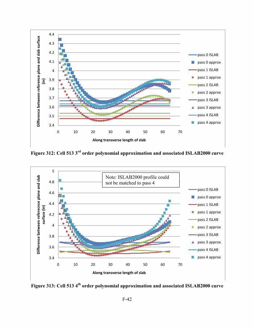
F-42
Figure 312: Cell 513 3rd order polynomial approximation and associated ISLAB2000 curve
Figure 313: Cell 513 4th order polynomial approximation and associated ISLAB2000 curve
3.4
3.5
3.6
3.7
3.8
3.9
4
4.1
4.2
4.3
4.4
0 10 20 30 40 50 60 70
Diff
eren
ce b
etw
een
refe
renc
e pl
ane
and
slab
sur
face
(in
)
Along transverse length of slab
pass 0 ISLAB
pass 0 approx
pass 1 ISLAB
pass 1 approx
pass 2 ISLAB
pass 2 approx
pass 3 ISLAB
pass 3 approx
pass 4 ISLAB
pass 4 approx
3.4
3.6
3.8
4
4.2
4.4
4.6
4.8
5
0 10 20 30 40 50 60 70
Diff
eren
ce b
etw
een
refe
recn
ce p
lane
and
sla
b su
rfac
e (in
)
Along transverse length of slab
pass 0 ISLAB
pass 0 approx
pass 1 ISLAB
pass 1 approx
pass 2 ISLAB
pass 2 approx
pass 3 ISLAB
pass 3 approx
pass 4 ISLAB
pass 4 approx
Note: ISLAB2000 profile could not be matched to pass 4

F-43
Figure 314: Cell 513 5th order polynomial approximation and associated ISLAB2000 curve
Figure 315: Cell 513 6th order polynomial approximation and associated ISLAB2000 curve
2.5
3
3.5
4
4.5
5
5.5
6
6.5
0 10 20 30 40 50 60 70
Diff
eren
ce b
etw
een
refe
renc
e pl
ane
and
slab
sur
face
(in
)
Along transverse length of slab
pass 0 ISLAB
pass 0 approx
pass 1 ISLAB
pass 1 approx
pass 2 ISLAB
pass 2 approx
pass 3 ISLAB
pass 3 approx
pass 4 ISLAB
pass 4 approx
1
1.5
2
2.5
3
3.5
4
4.5
5
0 10 20 30 40 50 60 70
Diff
eren
ce b
etw
een
refe
renc
e pl
ane
and
slab
su
rfac
e (in
)
Along transverse length of slab
pass 0 ISLAB
pass 0 approx
pass 1 ISLAB
pass 1 approx
pass 2 ISLAB
pass 2 approx
pass 3 ISLAB
pass 3 approx
pass 4 ISLAB
pass 4 approx
Note: ISLAB2000 profile could not be matched to passes 0, 1, 2, 3, or 4

F-44
Figure 316: Cell 614 2nd order polynomial approximation and associated ISLAB2000 curve
Figure 317: Cell 614 3rd order polynomial approximation and associated ISLAB2000 curve
2.8
3
3.2
3.4
3.6
3.8
4
4.2
0 10 20 30 40 50 60 70
Diff
eren
ce b
etw
een
refe
renc
e pl
ane
and
slab
su
rfac
e (in
)
Along transverse length of slab
pass 0 ISLAB
pass 0 approx
pass 1 ISLAB
pass 1 approx
pass 2 ISLAB
pass 2 approx
pass 3 ISLAB
pass 3 approx
pass 4 ISLAB
pass 4 approx
1.5
2
2.5
3
3.5
4
4.5
0 10 20 30 40 50 60 70
Diff
eren
ce b
etw
een
refe
renc
e pl
ane
and
slab
sur
face
(in
)
Along transverse length of slab
pass 0 ISLAB
pass 0 approx
pass 1 ISLAB
pass 1 approx
pass 2 ISLAB
pass 2 approx
pass 3 ISLAB
pass 3 approx
pass 4 ISLAB
pass 4 approx
Note: ISLAB2000 profile could not be matched to pass 4

F-45
Figure 318: Cell 614 4th order polynomial approximation and associated ISLAB2000 curve
Figure 319: Cell 614 5th order polynomial approximation and associated ISLAB2000 curve
-1.5
-0.5
0.5
1.5
2.5
3.5
4.5
0 10 20 30 40 50 60 70
Diff
eren
ce b
etw
een
refe
recn
ce p
lane
and
sla
b su
rfac
e (in
)
Along transverse length of slab
pass 0 ISLAB
pass 0 approx
pass 1 ISLAB
pass 1 approx
pass 2 ISLAB
pass 2 approx
pass 3 ISLAB
pass 3 approx
pass 4 ISLAB
pass 4 approx
-800
-700
-600
-500
-400
-300
-200
-100
0
100
200
0 10 20 30 40 50 60 70
Diff
eren
ce b
etw
een
refe
renc
e pl
ane
and
slab
su
rfac
e (in
)
Along transverse length of slab
pass 0 ISLAB
pass 0 approx
pass 1 ISLAB
pass 1 approx
pass 2 ISLAB
pass 2 approx
pass 3 ISLAB
pass 3 approx
pass 4 ISLAB
pass 4 approx
Note: ISLAB2000 profile could not be matched to passes 1, 2, or 3,
Note: ISLAB2000 profile could not be matched to pass 4
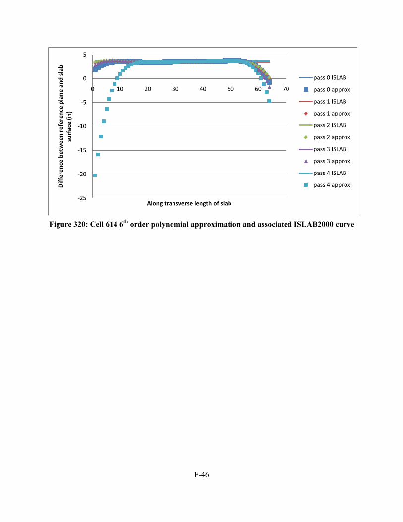
F-46
Figure 320: Cell 614 6th order polynomial approximation and associated ISLAB2000 curve
-25
-20
-15
-10
-5
0
5
0 10 20 30 40 50 60 70
Diff
eren
ce b
etw
een
refe
renc
e pl
ane
and
slab
su
rfac
e (in
)
Along transverse length of slab
pass 0 ISLAB
pass 0 approx
pass 1 ISLAB
pass 1 approx
pass 2 ISLAB
pass 2 approx
pass 3 ISLAB
pass 3 approx
pass 4 ISLAB
pass 4 approx

APPENDIX G: BUILT-IN CURL AS DETERMINED FROM THE POLYNOMIAL CURVATURE AND ΔH METHODS – WHOLE SLABS
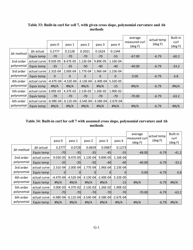
G-1
Table 33: Built-in curl for cell 7, with given cross slope, polynomial curvature and Δh methods
average
measured curl (deg F)
actual temp (deg F)
Built-in curl
(deg F)
pass 0 pass 1 pass 2 pass 3 pass 4
Δh method Δh actual 3.2777 0.2128 0.2021 0.1624 0.1344
Equiv temp -70 -70 -70 -70 -55 -67.00 -6.79 -60.2
2nd order polynomial
actual curve 9.03E-05 8.47E-05 1.13E-04 9.89E-05 1.16E-04 Equiv temp -35 -35 -50 -40 -40 -40.00 -6.79 -33.2
3rd order polynomial
actual curve 2.31E-04 2.00E-04 1.77E-04 1.96E-04 2.23E-04 Equiv temp 0 0 0 0 0 0.00 -6.79 6.8
4th order polynomial
actual curve -4.47E-04 -4.52E-04 -3.13E-04 -2.40E-04 5.32E-05 Equiv temp #N/A #N/A #N/A #N/A -15 #N/A -6.79 #N/A
5th order polynomial
actual curve 3.00E-03 4.37E-02 2.13E-03 1.26E-02 1.90E-02 Equiv temp -70 -70 -70 -70 -70 -70.00 -6.79 -63.2
6th order polynomial
actual curve -6.98E-04 -6.11E-04 -3.54E-04 -3.58E-04 -2.67E-04 Equiv temp #N/A #N/A #N/A #N/A #N/A #N/A -6.79 #N/A
Table 34: Built-in curl for cell 7 with assumed cross slope, polynomial curvature and Δh methods
average
measured curl (deg F)
actual temp (deg F)
Built-in curl
(deg F)
pass 0 pass 1 pass 2 pass 3 pass 4
Δh method Δh actual 3.2777 0.0728 0.0659 0.0987 0.1273
Equiv temp -70 -35 -35 -45 -55 -48.00 -6.79 -41.2
2nd order polynomial
actual curve 9.03E-05 8.47E-05 1.13E-04 9.89E-05 1.16E-04 Equiv temp -35 -35 -50 -40 -40 -40.00 -6.79 -33.2
3rd order polynomial
actual curve 2.31E-04 2.00E-04 1.77E-04 1.96E-04 2.23E-04 Equiv temp 0 0 0 0 0 0.00 -6.79 6.8
4th order polynomial
actual curve -4.47E-04 -4.52E-04 -3.13E-04 -2.40E-04 5.32E-05 Equiv temp #N/A #N/A #N/A #N/A -15 #N/A -6.79 #N/A
5th order polynomial
actual curve 3.00E-03 4.37E-02 2.13E-03 1.26E-02 1.90E-02 Equiv temp -70 -70 -70 -70 -70 -70.00 -6.79 -63.2
6th order polynomial
actual curve -6.98E-04 -6.11E-04 -3.54E-04 -3.58E-04 -2.67E-04 Equiv temp #N/A #N/A #N/A #N/A #N/A #N/A -6.79 #N/A

G-2
Table 35: Built-in curl for cell 12 with given cross slope, polynomial curvature and Δh methods
average
measured curl (deg F)
actual temp (deg F)
Built-in curl
(deg F)
pass 0 pass 1 pass 2 pass 3 pass 4
Δh method Δh actual 2.9374 0.3151 0.2784 0.2877 0.1956
Equiv temp -70 -70 -70 -70 -70 -70.00 -10.93 -59.1
2nd order polynomial
actual curve 3.51E-04 3.26E-04 2.32E-04 2.23E-04 1.37E-04 Equiv temp -70 -70 -70 -70 -55 -67.00 -10.93 -56.1
3rd order polynomial
actual curve 4.10E-04 4.02E-04 7.33E-05 3.18E-05 -2.01E-05 Equiv temp 0 0 0 0 5 1.00 -10.93 11.9
4th order polynomial
actual curve 2.18E-04 2.07E-04 -1.03E-04 -2.05E-04 -2.72E-04 Equiv temp -45 -45 25 #N/A #N/A #N/A -10.93 #N/A
5th order polynomial
actual curve 2.46E-02 1.98E-02 1.40E-02 2.78E-02 3.20E-02 Equiv temp -70 -70 -70 -70 -70 -70.00 -10.93 -59.1
6th order polynomial
actual curve -1.48E-03 -1.39E-03 -8.22E-04 -1.07E-03 -6.91E-04 Equiv temp #N/A #N/A #N/A #N/A #N/A #N/A -10.93 #N/A
Table 36: Built-in curl for cell 12 with assumed cross slope, polynomial curvature and Δh methods
average
measured curl (deg F)
actual temp (deg F)
Built-in curl
(deg F)
pass 0 pass 1 pass 2 pass 3 pass 4
Δh method Δh actual 2.9658 0.1366 0.1054 0.1092 0.0171
Equiv temp 0 0 0 0 15 3.00 -10.93 13.9
2nd order polynomial
actual curve 3.51E-04 3.26E-04 2.32E-04 2.23E-04 1.37E-04 Equiv temp -70 -70 -70 -70 -55 -67.00 -10.93 -56.1
3rd order polynomial
actual curve 4.10E-04 4.02E-04 7.33E-05 3.18E-05 -2.01E-05 Equiv temp 0 0 0 0 5 1.00 -10.93 11.9
4th order polynomial
actual curve 2.18E-04 2.07E-04 -1.03E-04 -2.05E-04 -2.72E-04 Equiv temp -45 -45 25 #N/A #N/A #N/A -10.93 #N/A
5th order polynomial
actual curve 2.46E-02 1.98E-02 1.40E-02 2.78E-02 3.20E-02 Equiv temp -70 -70 -70 -70 -70 -70.00 -10.93 -59.1
6th order polynomial
actual curve -1.48E-03 -1.39E-03 -8.22E-04 -1.07E-03 -6.91E-04 Equiv temp #N/A #N/A #N/A #N/A #N/A #N/A -10.93 #N/A

G-3
Table 37: Built-in curl for cell 36 panel 19 early morning test with given cross slope, polynomial curvature and Δh methods
average
measured curl (deg F)
actual temp (deg F)
Built-in curl
(deg F)
pass 0 pass 1 pass 2 pass 3 pass 4
Δh method Δh actual 2.7625 0.1628 0.1629 0.2168 0.1981
Equiv temp -70 -70 -70 -70 -70 -70.00 -10.2 -59.8
2nd order polynomial
actual curve 2.63E-04 1.52E-04 1.56E-04 2.53E-04 2.64E-04 Equiv temp -70 -45 -50 -70 -70 -61.00 -10.2 -50.8
3rd order polynomial
actual curve -5.24E-04 -4.53E-04 -6.09E-05 2.14E-04 -2.52E-04 Equiv temp 10 5 5 0 5 5.00 -10.2 15.2
4th order polynomial
actual curve 1.29E-03 1.75E-03 1.62E-03 1.79E-04 2.46E-04 Equiv temp -70 -70 -70 -30 -40 -56.00 -10.2 -45.8
5th order polynomial
actual curve 2.81E-03 7.08E-03 1.07E-02 2.35E-03 1.60E-03 Equiv temp -70 -70 -70 -70 -70 -70.00 -10.2 -59.8
6th order polynomial
actual curve 4.83E-03 4.10E-03 6.07E-03 5.98E-03 8.26E-03 Equiv temp -70 -70 -70 -70 -70 -70.00 -10.2 -59.8
Table 38: Built-in curl for cell 36 panel 19 early morning test with assumed cross slope, polynomial curvature and Δh methods
average
measured curl (deg F)
actual temp (deg F)
Built-in curl
(deg F)
pass 0 pass 1 pass 2 pass 3 pass 4
Δh method Δh actual 2.7625 0.0731 0.0854 0.1218 0.1495
Equiv temp -70 -40 -45 -55 -70 -56.00 -10.2 -45.8
2nd order polynomial
actual curve 2.63E-04 1.52E-04 1.56E-04 2.53E-04 2.64E-04 Equiv temp -70 -45 -50 -70 -70 -61.00 -10.2 -50.8
3rd order polynomial
actual curve -5.24E-04 -4.53E-04 -6.09E-05 2.14E-04 -2.52E-04 Equiv temp 10 5 5 0 5 5.00 -10.2 15.2
4th order polynomial
actual curve 1.29E-03 1.75E-03 1.62E-03 1.79E-04 2.46E-04 Equiv temp -70 -70 -70 -30 -40 -56.00 -10.2 -45.8
5th order polynomial
actual curve 2.81E-03 7.08E-03 1.07E-02 2.35E-03 1.60E-03 Equiv temp -70 -70 -70 -70 -70 -70.00 -10.2 -59.8
6th order polynomial
actual curve 4.83E-03 4.10E-03 6.07E-03 5.98E-03 8.26E-03 Equiv temp -70 -70 -70 -70 -70 -70.00 -10.2 -59.8
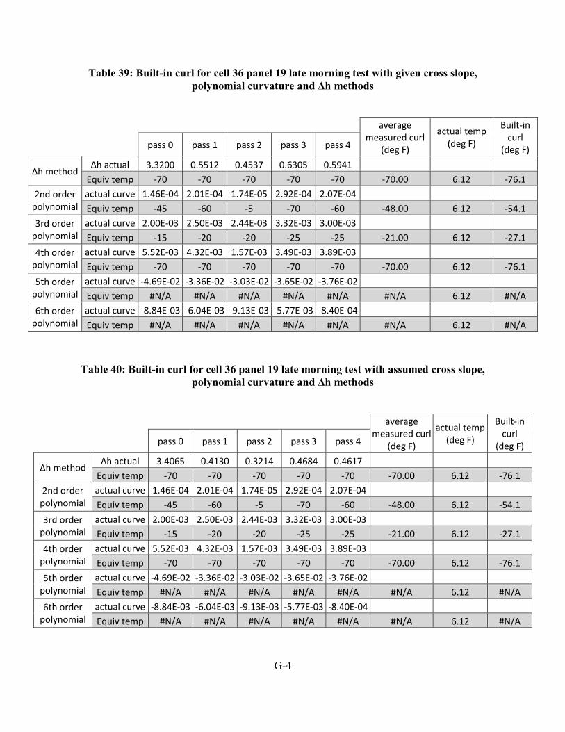
G-4
Table 39: Built-in curl for cell 36 panel 19 late morning test with given cross slope, polynomial curvature and Δh methods
average
measured curl (deg F)
actual temp (deg F)
Built-in curl
(deg F)
pass 0 pass 1 pass 2 pass 3 pass 4
Δh method Δh actual 3.3200 0.5512 0.4537 0.6305 0.5941
Equiv temp -70 -70 -70 -70 -70 -70.00 6.12 -76.1
2nd order polynomial
actual curve 1.46E-04 2.01E-04 1.74E-05 2.92E-04 2.07E-04 Equiv temp -45 -60 -5 -70 -60 -48.00 6.12 -54.1
3rd order polynomial
actual curve 2.00E-03 2.50E-03 2.44E-03 3.32E-03 3.00E-03 Equiv temp -15 -20 -20 -25 -25 -21.00 6.12 -27.1
4th order polynomial
actual curve 5.52E-03 4.32E-03 1.57E-03 3.49E-03 3.89E-03 Equiv temp -70 -70 -70 -70 -70 -70.00 6.12 -76.1
5th order polynomial
actual curve -4.69E-02 -3.36E-02 -3.03E-02 -3.65E-02 -3.76E-02 Equiv temp #N/A #N/A #N/A #N/A #N/A #N/A 6.12 #N/A
6th order polynomial
actual curve -8.84E-03 -6.04E-03 -9.13E-03 -5.77E-03 -8.40E-04 Equiv temp #N/A #N/A #N/A #N/A #N/A #N/A 6.12 #N/A
Table 40: Built-in curl for cell 36 panel 19 late morning test with assumed cross slope, polynomial curvature and Δh methods
average
measured curl (deg F)
actual temp (deg F)
Built-in curl
(deg F)
pass 0 pass 1 pass 2 pass 3 pass 4
Δh method Δh actual 3.4065 0.4130 0.3214 0.4684 0.4617
Equiv temp -70 -70 -70 -70 -70 -70.00 6.12 -76.1
2nd order polynomial
actual curve 1.46E-04 2.01E-04 1.74E-05 2.92E-04 2.07E-04 Equiv temp -45 -60 -5 -70 -60 -48.00 6.12 -54.1
3rd order polynomial
actual curve 2.00E-03 2.50E-03 2.44E-03 3.32E-03 3.00E-03 Equiv temp -15 -20 -20 -25 -25 -21.00 6.12 -27.1
4th order polynomial
actual curve 5.52E-03 4.32E-03 1.57E-03 3.49E-03 3.89E-03 Equiv temp -70 -70 -70 -70 -70 -70.00 6.12 -76.1
5th order polynomial
actual curve -4.69E-02 -3.36E-02 -3.03E-02 -3.65E-02 -3.76E-02 Equiv temp #N/A #N/A #N/A #N/A #N/A #N/A 6.12 #N/A
6th order polynomial
actual curve -8.84E-03 -6.04E-03 -9.13E-03 -5.77E-03 -8.40E-04 Equiv temp #N/A #N/A #N/A #N/A #N/A #N/A 6.12 #N/A

G-5
Table 41: Built-in curl for cell 36 panel 20 early morning test with given cross slope, polynomial curvature and Δh methods
average
measured curl (deg F)
actual temp (deg F)
Built-in curl
(deg F)
pass 0 pass 1 pass 2 pass 3 pass 4
Δh method Δh actual 0.1695 0.0675 0.2048 0.2905 0.2692
Equiv temp -70 -35 -70 -70 -70 -63.00 -10.2 -52.8
2nd order polynomial
actual curve 2.33E-04 1.08E-04 1.40E-04 2.20E-04 1.91E-04 Equiv temp -70 -35 -45 -65 -55 -54.00 -10.2 -43.8
3rd order polynomial
actual curve 1.87E-05 2.72E-04 -6.23E-05 -5.83E-04 -5.91E-04 Equiv temp 0 0 5 10 10 5.00 -10.2 15.2
4th order polynomial
actual curve 1.41E-04 3.64E-04 -6.03E-05 -4.89E-04 -7.48E-04 Equiv temp -25 -55 15 #N/A #N/A #N/A -10.2 #N/A
5th order polynomial
actual curve -2.65E-04 2.81E-03 -2.41E-03 -7.12E-03 -9.18E-03 Equiv temp #N/A -70 #N/A #N/A #N/A #N/A -10.2 #N/A
6th order polynomial
actual curve 1.78E-04 6.79E-04 -3.12E-04 -1.11E-03 -1.80E-03 Equiv temp -30 -70 #N/A #N/A #N/A #N/A -10.2 #N/A
Table 42: Built-in curl for cell 36 panel 20 early morning test with assumed cross slope, polynomial curvature and Δh methods
average
measured curl (deg F)
actual temp (deg F)
Built-in curl
(deg F)
pass 0 pass 1 pass 2 pass 3 pass 4
Δh method Δh actual 0.1317 0.0205 0.1328 0.2185 0.1972
Equiv temp -65 -15 -70 -70 -70 -58.00 -10.2 -47.8
2nd order polynomial
actual curve 2.33E-04 1.08E-04 1.40E-04 2.20E-04 1.91E-04 Equiv temp -70 -35 -45 -65 -55 -54.00 -10.2 -43.8
3rd order polynomial
actual curve 1.87E-05 2.72E-04 -6.23E-05 -5.83E-04 -5.91E-04 Equiv temp 0 0 5 10 10 5.00 -10.2 15.2
4th order polynomial
actual curve 1.41E-04 3.64E-04 -6.03E-05 -4.89E-04 -7.48E-04 Equiv temp -25 -55 15 #N/A #N/A #N/A -10.2 #N/A
5th order polynomial
actual curve -2.65E-04 2.81E-03 -2.41E-03 -7.12E-03 -9.18E-03 Equiv temp #N/A -70 #N/A #N/A #N/A #N/A -10.2 #N/A
6th order polynomial
actual curve 1.78E-04 6.79E-04 -3.12E-04 -1.11E-03 -1.80E-03 Equiv temp -30 -70 #N/A #N/A #N/A #N/A -10.2 #N/A
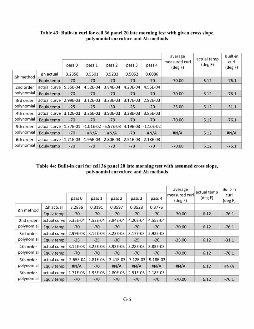
G-6
Table 43: Built-in curl for cell 36 panel 20 late morning test with given cross slope, polynomial curvature and Δh methods
average
measured curl (deg F)
actual temp (deg F)
Built-in curl
(deg F)
pass 0 pass 1 pass 2 pass 3 pass 4
Δh method Δh actual 3.2358 0.5501 0.5232 0.5052 0.6086
Equiv temp -70 -70 -70 -70 -70 -70.00 6.12 -76.1
2nd order polynomial
actual curve 5.35E-04 4.52E-04 3.84E-04 4.20E-04 4.55E-04 Equiv temp -70 -70 -70 -70 -70 -70.00 6.12 -76.1
3rd order polynomial
actual curve 2.99E-03 3.12E-03 3.23E-03 3.17E-03 2.92E-03 Equiv temp -25 -25 -30 -25 -20 -25.00 6.12 -31.1
4th order polynomial
actual curve 3.12E-03 3.25E-03 3.93E-03 3.28E-03 3.85E-03 Equiv temp -70 -70 -70 -70 -70 -70.00 6.12 -76.1
5th order polynomial
actual curve 1.37E-01 -1.01E-02 -5.57E-03 4.19E-03 -1.10E-02 Equiv temp -70 #N/A #N/A -70 #N/A #N/A 6.12 #N/A
6th order polynomial
actual curve 1.71E-03 1.95E-03 2.80E-03 2.51E-03 2.18E-03 Equiv temp -70 -70 -70 -70 -70 -70.00 6.12 -76.1
Table 44: Built-in curl for cell 36 panel 20 late morning test with assumed cross slope, polynomial curvature and Δh methods
average
measured curl (deg F)
actual temp (deg F)
Built-in curl
(deg F)
pass 0 pass 1 pass 2 pass 3 pass 4
Δh method Δh actual 3.2836 0.3191 0.3597 0.3528 0.3776
Equiv temp -70 -70 -70 -70 -70 -70.00 6.12 -76.1
2nd order polynomial
actual curve 5.35E-04 4.52E-04 3.84E-04 4.20E-04 4.55E-04 Equiv temp -70 -70 -70 -70 -70 -70.00 6.12 -76.1
3rd order polynomial
actual curve 2.99E-03 3.12E-03 3.23E-03 3.17E-03 2.92E-03 Equiv temp -25 -25 -30 -25 -20 -25.00 6.12 -31.1
4th order polynomial
actual curve 3.12E-03 3.25E-03 3.93E-03 3.28E-03 3.85E-03 Equiv temp -70 -70 -70 -70 -70 -70.00 6.12 -76.1
5th order polynomial
actual curve -2.65E-04 2.81E-03 -2.41E-03 -7.12E-03 -9.18E-03 Equiv temp #N/A -70 #N/A #N/A #N/A #N/A 6.12 #N/A
6th order polynomial
actual curve 1.71E-03 1.95E-03 2.80E-03 2.51E-03 2.18E-03 Equiv temp -70 -70 -70 -70 -70 -70.00 6.12 -76.1

G-7
Table 45: Built-in curl for cell 37 panel 8 early morning test with given cross slope, polynomial curvature and Δh methods
average
measured curl (deg F)
actual temp (deg F)
Built-in curl
(deg F)
pass 0 pass 1 pass 2 pass 3 pass 4
Δh method Δh actual 2.6415 0.2909 0.0948 0.2942 0.2213
Equiv temp -70 -70 -50 0 -70 -52.00 -10.43 -41.6
2nd order polynomial
actual curve 2.87E-04 2.98E-04 2.18E-04 3.60E-04 3.36E-04 Equiv temp -70 -70 -65 -70 -70 -69.00 -10.43 -58.6
3rd order polynomial
actual curve -1.02E-03 -1.22E-03 -7.25E-04 -1.40E-03 -6.77E-04 Equiv temp 10 10 10 15 10 11.00 -10.43 21.4
4th order polynomial
actual curve -5.76E-04 -2.88E-04 -7.06E-04 -9.12E-05 -1.65E-04 Equiv temp #N/A #N/A #N/A 20 #N/A #N/A -10.43 #N/A
5th order polynomial
actual curve -8.32E-03 -1.40E-02 -2.65E-03 -1.17E-02 -4.96E-03 Equiv temp #N/A #N/A #N/A #N/A #N/A #N/A -10.43 #N/A
6th order polynomial
actual curve -1.01E-03 -1.15E-03 -6.18E-04 -2.28E-04 -2.61E-04 Equiv temp #N/A #N/A #N/A #N/A #N/A #N/A -10.43 #N/A
Table 46: Built-in curl for cell 37 panel 8 early morning test with assumed cross slope, polynomial curvature and Δh methods
average
measured curl (deg F)
actual temp (deg F)
Built-in curl
(deg F)
pass 0 pass 1 pass 2 pass 3 pass 4
Δh method Δh actual 2.6415 0.3569 0.1454 0.3602 0.2793
Equiv temp -70 -70 -70 -70 -70 -70.00 -10.43 -59.6
2nd order polynomial
actual curve 2.87E-04 2.98E-04 2.18E-04 3.60E-04 3.36E-04 Equiv temp -70 -70 -65 -70 -70 -69.00 -10.43 -58.6
3rd order polynomial
actual curve -1.02E-03 -1.22E-03 -7.25E-04 -1.40E-03 -6.77E-04 Equiv temp 10 10 10 15 10 11.00 -10.43 21.4
4th order polynomial
actual curve -5.76E-04 -2.88E-04 -7.06E-04 -9.12E-05 -1.65E-04 Equiv temp #N/A #N/A #N/A 20 #N/A #N/A -10.43 #N/A
5th order polynomial
actual curve -8.32E-03 -1.40E-02 -2.65E-03 -1.17E-02 -4.96E-03 Equiv temp #N/A #N/A #N/A #N/A #N/A #N/A -10.43 #N/A
6th order polynomial
actual curve -1.01E-03 -1.15E-03 -6.18E-04 -2.28E-04 -2.61E-04 Equiv temp #N/A #N/A #N/A #N/A #N/A #N/A -10.43 #N/A

G-8
Table 47: Built-in curl for cell 37 panel 8 late morning test with given cross slope, polynomial curvature and Δh methods
average
measured curl (deg F)
actual temp (deg F)
Built-in curl
(deg F)
pass 0 pass 1 pass 2 pass 3 pass 4
Δh method Δh actual 3.4791 0.6188 0.3668 0.6562 0.3740
Equiv temp -70 -70 -70 0 -70 -56.00 9.75 -65.8
2nd order polynomial
actual curve 3.41E-04 3.84E-04 2.76E-04 4.45E-04 2.80E-04 Equiv temp -70 -70 -70 -70 -70 -70.00 9.75 -79.8
3rd order polynomial
actual curve 5.39E-04 9.95E-04 1.27E-03 3.27E-04 7.87E-04 Equiv temp -5 -5 -10 0 -5 -5.00 9.75 -14.8
4th order polynomial
actual curve 1.73E-03 2.67E-03 1.63E-03 2.50E-03 1.69E-03 Equiv temp -70 -70 -70 -70 -70 -70.00 9.75 -79.8
5th order polynomial
actual curve -3.25E-02 -3.18E-02 -1.83E-02 -3.53E-02 -2.40E-02 Equiv temp #N/A #N/A #N/A #N/A #N/A #N/A 9.75 #N/A
6th order polynomial
actual curve -1.66E-03 -5.23E-04 -4.55E-04 -2.68E-04 -5.19E-04 Equiv temp #N/A #N/A #N/A #N/A #N/A #N/A 9.75 #N/A
Table 48: Built-in curl for cell 37 panel 8 late morning test with assumed cross slope, polynomial curvature and Δh methods
average
measured curl (deg F)
actual temp (deg F)
Built-in curl
(deg F)
pass 0 pass 1 pass 2 pass 3 pass 4
Δh method Δh actual 3.4791 0.2888 0.0781 0.3262 0.0576
Equiv temp -70 -70 -45 -70 -30 -57.00 9.75 -66.8
2nd order polynomial
actual curve 3.41E-04 3.84E-04 2.76E-04 4.45E-04 2.80E-04 Equiv temp -70 -70 -70 -70 -70 -70.00 9.75 -79.8
3rd order polynomial
actual curve 5.39E-04 9.95E-04 1.27E-03 3.27E-04 7.87E-04 Equiv temp -5 -5 -10 0 -5 -5.00 9.75 -14.8
4th order polynomial
actual curve 1.73E-03 2.67E-03 1.63E-03 2.50E-03 1.69E-03 Equiv temp -70 -70 -70 -70 -70 -70.00 9.75 -79.8
5th order polynomial
actual curve -3.25E-02 -3.18E-02 -1.83E-02 -3.53E-02 -2.40E-02 Equiv temp #N/A #N/A #N/A #N/A #N/A #N/A 9.75 #N/A
6th order polynomial
actual curve -1.66E-03 -5.23E-04 -4.55E-04 -2.68E-04 -5.19E-04 Equiv temp #N/A #N/A #N/A #N/A #N/A #N/A 9.75 #N/A

G-9
Table 49: Built-in curl for cell 37 panel 9 early morning test with given cross slope, polynomial curvature and Δh methods
average
measured curl (deg F)
actual temp (deg F)
Built-in curl
(deg F)
pass 0 pass 1 pass 2 pass 3 pass 4
Δh method Δh actual 2.6056 0.2187 0.2973 0.3047 0.2735
Equiv temp -70 -70 -70 0 -70 -56.00 -10.43 -45.6
2nd order polynomial
actual curve 1.60E-04 2.16E-04 3.22E-04 2.85E-04 3.21E-04 Equiv temp -50 -65 -70 -70 -70 -65.00 -10.43 -54.6
3rd order polynomial
actual curve -7.38E-04 -9.54E-04 -1.19E-03 -1.01E-03 -1.09E-03 Equiv temp 10 10 10 10 10 10.00 -10.43 20.4
4th order polynomial
actual curve -3.96E-05 -7.41E-04 -4.04E-04 -2.70E-04 -3.41E-04 Equiv temp 15 #N/A #N/A #N/A #N/A #N/A -10.43 #N/A
5th order polynomial
actual curve -1.53E-02 -1.22E-02 -2.01E-02 -5.68E-03 -9.21E-03 Equiv temp #N/A #N/A #N/A #N/A #N/A #N/A -10.43 #N/A
6th order polynomial
actual curve -1.26E-03 -2.14E-03 -2.21E-03 -3.47E-04 -6.74E-04 Equiv temp #N/A #N/A #N/A #N/A #N/A #N/A -10.43 #N/A
Table 50: Built-in curl for cell 37 panel 9 early morning test with assumed cross slope, polynomial curvature and Δh methods
average
measured curl (deg F)
actual temp (deg F)
Built-in curl
(deg F)
pass 0 pass 1 pass 2 pass 3 pass 4
Δh method Δh actual 2.6056 0.2407 0.3193 0.3267 0.2955
Equiv temp -70 -70 -70 -70 -70 -70.00 -10.43 -59.6
2nd order polynomial
actual curve 1.60E-04 2.16E-04 3.22E-04 2.85E-04 3.21E-04 Equiv temp -50 -65 -70 -70 -70 -65.00 -10.43 -54.6
3rd order polynomial
actual curve -7.38E-04 -9.54E-04 -1.19E-03 -1.01E-03 -1.09E-03 Equiv temp 10 10 10 10 10 10.00 -10.43 20.4
4th order polynomial
actual curve -3.96E-05 -7.41E-04 -4.04E-04 -2.70E-04 -3.41E-04 Equiv temp 15 #N/A #N/A #N/A #N/A #N/A -10.43 #N/A
5th order polynomial
actual curve -1.53E-02 -1.22E-02 -2.01E-02 -5.68E-03 -9.21E-03 Equiv temp #N/A #N/A #N/A #N/A #N/A #N/A -10.43 #N/A
6th order polynomial
actual curve -1.26E-03 -2.14E-03 -2.21E-03 -3.47E-04 -6.74E-04 Equiv temp #N/A #N/A #N/A #N/A #N/A #N/A -10.43 #N/A

G-10
Table 51: Built-in curl for cell 37 panel 9 late morning test with given cross slope, polynomial curvature and Δh methods
average
measured curl (deg F)
actual temp (deg F)
Built-in curl
(deg F)
pass 0 pass 1 pass 2 pass 3 pass 4
Δh method Δh actual 3.4319 0.5236 0.7123 0.5965 0.5985
Equiv temp -70 -70 -70 -70 -70 -70.00 9.75 -79.8
2nd order polynomial
actual curve 2.67E-04 2.38E-04 3.91E-04 3.56E-04 3.76E-04 Equiv temp -70 -70 -70 -70 -70 -70.00 9.75 -79.8
3rd order polynomial
actual curve 1.31E-03 1.03E-03 8.68E-04 6.64E-04 7.68E-04 Equiv temp -10 -5 -5 -5 -5 -6.00 9.75 -15.8
4th order polynomial
actual curve 2.91E-03 1.10E-03 2.46E-03 1.96E-03 2.13E-03 Equiv temp -70 -70 -70 -70 -70 -70.00 9.75 -79.8
5th order polynomial
actual curve -3.49E-02 -2.71E-02 -2.95E-02 -2.70E-02 -2.90E-02 Equiv temp #N/A #N/A #N/A #N/A #N/A #N/A 9.75 #N/A
6th order polynomial
actual curve -8.34E-04 -2.61E-03 -7.67E-04 -7.26E-04 -6.89E-04 Equiv temp #N/A #N/A #N/A #N/A #N/A #N/A 9.75 #N/A
Table 52: Built-in curl cell 37 panel 9 late morning test with assumed cross slope, polynomial curvature and Δh methods
average
measured curl (deg F)
actual temp (deg F)
Built-in curl
(deg F)
pass 0 pass 1 pass 2 pass 3 pass 4
Δh method Δh actual 3.4406 0.1716 0.3603 0.2445 0.2465
Equiv temp -70 -70 -70 -70 -70 -70.00 9.75 -79.8
2nd order polynomial
actual curve 2.67E-04 2.38E-04 3.91E-04 3.56E-04 3.76E-04 Equiv temp -70 -70 -70 -70 -70 -70.00 9.75 -79.8
3rd order polynomial
actual curve 1.31E-03 1.03E-03 8.68E-04 6.64E-04 7.68E-04 Equiv temp -10 -5 -5 -5 -5 -6.00 9.75 -15.8
4th order polynomial
actual curve 2.91E-03 1.10E-03 2.46E-03 1.96E-03 2.13E-03 Equiv temp -70 -70 -70 -70 -70 -70.00 9.75 -79.8
5th order polynomial
actual curve -3.49E-02 -2.71E-02 -2.95E-02 -2.70E-02 -2.90E-02 Equiv temp #N/A #N/A #N/A #N/A #N/A #N/A 9.75 #N/A
6th order polynomial
actual curve -8.34E-04 -2.61E-03 -7.67E-04 -7.26E-04 -6.89E-04 Equiv temp #N/A #N/A #N/A #N/A #N/A #N/A 9.75 #N/A

G-11
Table 53: Built-in curl for cell 53 early morning test with given cross slope, polynomial curvature and Δh methods
average
measured curl (deg F)
actual temp (deg F)
Built-in curl
(deg F)
pass 0 pass 1 pass 2 pass 3 pass 4
Δh method Δh actual 2.4672 0.3440 0.4025 0.7126 0.4504
Equiv temp -70 -70 -70 0 -70 -56.00 -16.37 -39.6
2nd order polynomial
actual curve -5.18E-05 -1.15E-05 8.96E-05 4.24E-04 -5.55E-05 Equiv temp #N/A 10 -45 -70 #N/A #N/A -16.37 #N/A
3rd order polynomial
actual curve 1.89E-04 1.42E-04 -1.05E-04 1.92E-04 -3.29E-04 Equiv temp 0 0 5 0 5 2.00 -16.37 18.4
4th order polynomial
actual curve 7.96E-04 6.79E-04 1.85E-03 -4.71E-04 -1.10E-04 Equiv temp -70 -70 -70 #N/A #N/A #N/A -16.37 #N/A
5th order polynomial
actual curve -1.15E-02 -1.42E-02 3.93E-03 1.14E-02 -4.34E-03 Equiv temp #N/A #N/A -70 -70 #N/A #N/A -16.37 #N/A
6th order polynomial
actual curve -2.00E-04 -8.76E-04 3.83E-03 3.68E-04 -7.78E-04 Equiv temp #N/A #N/A -70 -70 #N/A #N/A -16.37 #N/A
Table 54: Built-in curl for cell 53 early morning test with assumed cross slope, polynomial curvature and Δh methods
average
measured curl (deg F)
actual temp (deg F)
Built-in curl
(deg F)
pass 0 pass 1 pass 2 pass 3 pass 4
Δh method Δh actual 2.5388 0.0994 0.0505 0.3606 0.0984
Equiv temp -70 -70 -45 -70 -70 -65.00 -16.37 -48.6
2nd order polynomial
actual curve -5.18E-05 -1.15E-05 8.96E-05 4.24E-04 -5.55E-05 Equiv temp #N/A 10 -45 -70 #N/A #N/A -16.37 #N/A
3rd order polynomial
actual curve 1.89E-04 1.42E-04 -1.05E-04 1.92E-04 -3.29E-04 Equiv temp 0 0 5 0 5 2.00 -16.37 18.4
4th order polynomial
actual curve 7.96E-04 6.79E-04 1.85E-03 -4.71E-04 -1.10E-04 Equiv temp -70 -70 -70 #N/A #N/A #N/A -16.37 #N/A
5th order polynomial
actual curve -1.15E-02 -1.42E-02 3.93E-03 1.14E-02 -4.34E-03 Equiv temp #N/A #N/A -70 -70 #N/A #N/A -16.37 #N/A
6th order polynomial
actual curve -2.00E-04 -8.76E-04 3.83E-03 3.68E-04 -7.78E-04 Equiv temp #N/A #N/A -70 -70 #N/A #N/A -16.37 #N/A

G-12
Table 55: built-in curl for cell 53 late morning test with given cross slope, polynomial curvature and Δh methods
average
measured curl (deg F)
actual temp (deg F)
Built-in curl
(deg F)
pass 0 pass 1 pass 2 pass 3 pass 4
Δh method Δh actual 3.2316 0.7317 0.7684 1.0863 0.8268
Equiv temp -70 -70 -70 0 -70 -56.00 7.03 -63.0
2nd order polynomial
actual curve -1.52E-04 2.91E-05 1.03E-04 3.72E-04 -6.38E-05 Equiv temp #N/A -15 -55 -70 #N/A #N/A 7.03 #N/A
3rd order polynomial
actual curve -2.19E-04 -3.65E-05 -1.34E-04 2.79E-05 -2.63E-04 Equiv temp 5 5 5 0 5 4.00 7.03 -3.0
4th order polynomial
actual curve 6.07E-04 1.64E-03 2.74E-03 5.88E-04 6.87E-04 Equiv temp -70 -70 -70 -70 -70 -70.00 8.03 -78.0
5th order polynomial
actual curve -9.65E-03 -1.49E-02 3.41E-03 7.15E-03 -3.59E-03 Equiv temp #N/A #N/A -70 -70 #N/A #N/A 7.03 #N/A
6th order polynomial
actual curve 4.59E-04 7.12E-04 5.22E-03 1.76E-03 1.85E-04 Equiv temp -70 -70 -70 -70 -45 -65.00 9.03 -74.0
Table 56: Built-in curl for cell 53 late morning test with assumed cross slope, polynomial curvature and Δh methods
average
measured curl (deg F)
actual temp (deg F)
Built-in curl
(deg F)
pass 0 pass 1 pass 2 pass 3 pass 4
Δh method Δh actual 3.3110 0.1156 0.1304 0.4482 0.1888
Equiv temp -70 -70 -70 -70 -70 -70.00 7.03 -63.0
2nd order polynomial
actual curve -1.52E-04 2.91E-05 1.03E-04 3.72E-04 -6.38E-05 Equiv temp #N/A -15 -55 -70 #N/A #N/A 7.03 #N/A
3rd order polynomial
actual curve -2.19E-04 -3.65E-05 -1.34E-04 2.79E-05 -2.63E-04 Equiv temp 5 5 5 0 5 4.00 7.03 -3.0
4th order polynomial
actual curve 6.07E-04 1.64E-03 2.74E-03 5.88E-04 6.87E-04 Equiv temp -70 -70 -70 -70 -70 -70.00 7.03 -77.0
5th order polynomial
actual curve -9.65E-03 -1.49E-02 3.41E-03 7.15E-03 -3.59E-03 Equiv temp #N/A #N/A -70 -70 #N/A #N/A 7.03 #N/A
6th order polynomial
actual curve 4.59E-04 7.12E-04 5.22E-03 1.76E-03 1.85E-04 Equiv temp -70 -70 -70 -70 -45 -65.00 7.03 -72.0
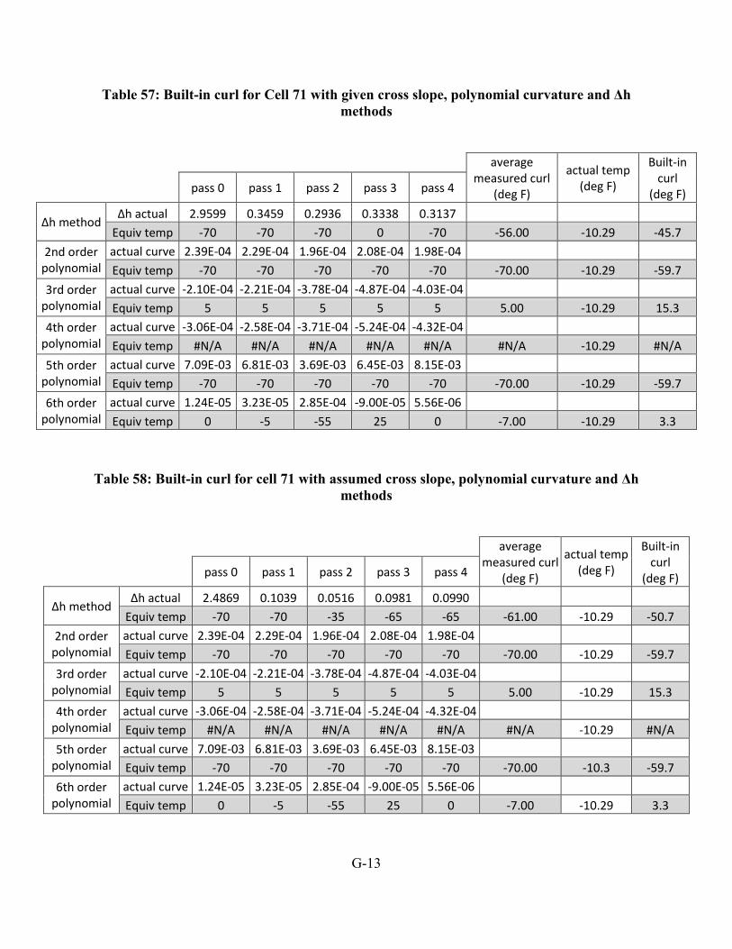
G-13
Table 57: Built-in curl for Cell 71 with given cross slope, polynomial curvature and Δh methods
average
measured curl (deg F)
actual temp (deg F)
Built-in curl
(deg F)
pass 0 pass 1 pass 2 pass 3 pass 4
Δh method Δh actual 2.9599 0.3459 0.2936 0.3338 0.3137
Equiv temp -70 -70 -70 0 -70 -56.00 -10.29 -45.7
2nd order polynomial
actual curve 2.39E-04 2.29E-04 1.96E-04 2.08E-04 1.98E-04 Equiv temp -70 -70 -70 -70 -70 -70.00 -10.29 -59.7
3rd order polynomial
actual curve -2.10E-04 -2.21E-04 -3.78E-04 -4.87E-04 -4.03E-04 Equiv temp 5 5 5 5 5 5.00 -10.29 15.3
4th order polynomial
actual curve -3.06E-04 -2.58E-04 -3.71E-04 -5.24E-04 -4.32E-04 Equiv temp #N/A #N/A #N/A #N/A #N/A #N/A -10.29 #N/A
5th order polynomial
actual curve 7.09E-03 6.81E-03 3.69E-03 6.45E-03 8.15E-03 Equiv temp -70 -70 -70 -70 -70 -70.00 -10.29 -59.7
6th order polynomial
actual curve 1.24E-05 3.23E-05 2.85E-04 -9.00E-05 5.56E-06 Equiv temp 0 -5 -55 25 0 -7.00 -10.29 3.3
Table 58: Built-in curl for cell 71 with assumed cross slope, polynomial curvature and Δh methods
average
measured curl (deg F)
actual temp (deg F)
Built-in curl
(deg F)
pass 0 pass 1 pass 2 pass 3 pass 4
Δh method Δh actual 2.4869 0.1039 0.0516 0.0981 0.0990
Equiv temp -70 -70 -35 -65 -65 -61.00 -10.29 -50.7
2nd order polynomial
actual curve 2.39E-04 2.29E-04 1.96E-04 2.08E-04 1.98E-04 Equiv temp -70 -70 -70 -70 -70 -70.00 -10.29 -59.7
3rd order polynomial
actual curve -2.10E-04 -2.21E-04 -3.78E-04 -4.87E-04 -4.03E-04 Equiv temp 5 5 5 5 5 5.00 -10.29 15.3
4th order polynomial
actual curve -3.06E-04 -2.58E-04 -3.71E-04 -5.24E-04 -4.32E-04 Equiv temp #N/A #N/A #N/A #N/A #N/A #N/A -10.29 #N/A
5th order polynomial
actual curve 7.09E-03 6.81E-03 3.69E-03 6.45E-03 8.15E-03 Equiv temp -70 -70 -70 -70 -70 -70.00 -10.3 -59.7
6th order polynomial
actual curve 1.24E-05 3.23E-05 2.85E-04 -9.00E-05 5.56E-06 Equiv temp 0 -5 -55 25 0 -7.00 -10.29 3.3
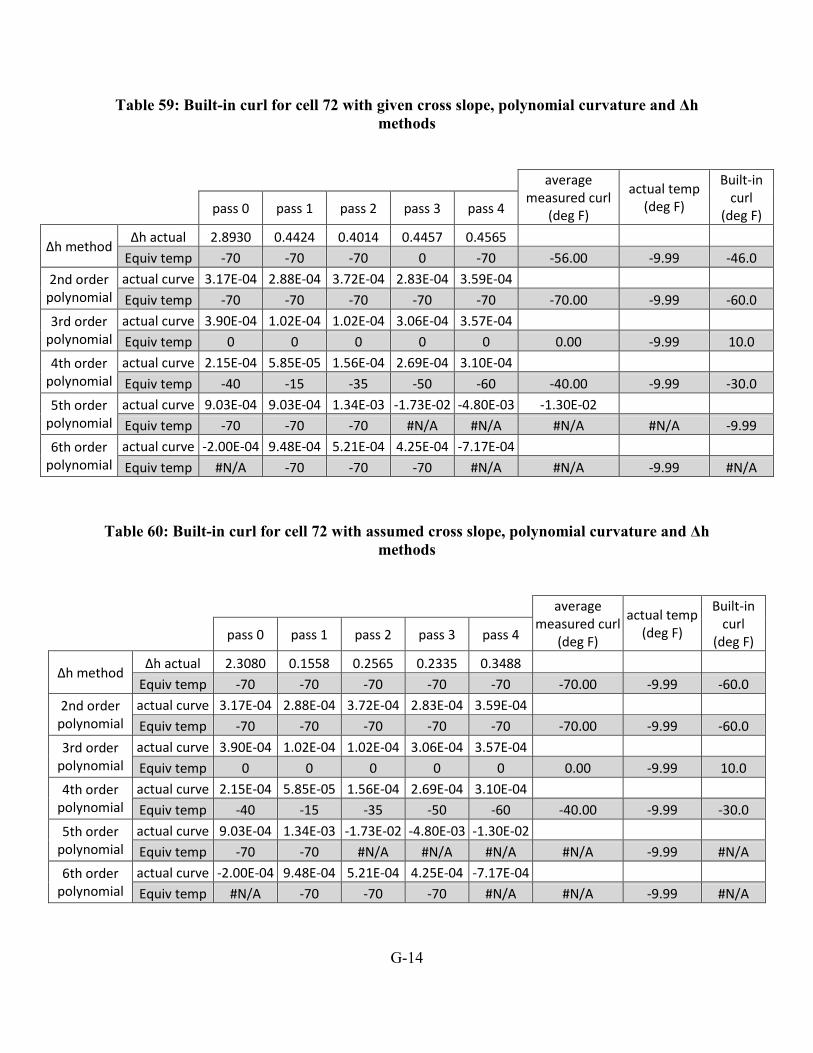
G-14
Table 59: Built-in curl for cell 72 with given cross slope, polynomial curvature and Δh methods
average
measured curl (deg F)
actual temp (deg F)
Built-in curl
(deg F)
pass 0 pass 1 pass 2 pass 3 pass 4
Δh method Δh actual 2.8930 0.4424 0.4014 0.4457 0.4565
Equiv temp -70 -70 -70 0 -70 -56.00 -9.99 -46.0
2nd order polynomial
actual curve 3.17E-04 2.88E-04 3.72E-04 2.83E-04 3.59E-04 Equiv temp -70 -70 -70 -70 -70 -70.00 -9.99 -60.0
3rd order polynomial
actual curve 3.90E-04 1.02E-04 1.02E-04 3.06E-04 3.57E-04 Equiv temp 0 0 0 0 0 0.00 -9.99 10.0
4th order polynomial
actual curve 2.15E-04 5.85E-05 1.56E-04 2.69E-04 3.10E-04 Equiv temp -40 -15 -35 -50 -60 -40.00 -9.99 -30.0
5th order polynomial
actual curve 9.03E-04 9.03E-04 1.34E-03 -1.73E-02 -4.80E-03 -1.30E-02 Equiv temp -70 -70 -70 #N/A #N/A #N/A #N/A -9.99
6th order polynomial
actual curve -2.00E-04 9.48E-04 5.21E-04 4.25E-04 -7.17E-04 Equiv temp #N/A -70 -70 -70 #N/A #N/A -9.99 #N/A
Table 60: Built-in curl for cell 72 with assumed cross slope, polynomial curvature and Δh methods
average
measured curl (deg F)
actual temp (deg F)
Built-in curl
(deg F)
pass 0 pass 1 pass 2 pass 3 pass 4
Δh method Δh actual 2.3080 0.1558 0.2565 0.2335 0.3488
Equiv temp -70 -70 -70 -70 -70 -70.00 -9.99 -60.0
2nd order polynomial
actual curve 3.17E-04 2.88E-04 3.72E-04 2.83E-04 3.59E-04 Equiv temp -70 -70 -70 -70 -70 -70.00 -9.99 -60.0
3rd order polynomial
actual curve 3.90E-04 1.02E-04 1.02E-04 3.06E-04 3.57E-04 Equiv temp 0 0 0 0 0 0.00 -9.99 10.0
4th order polynomial
actual curve 2.15E-04 5.85E-05 1.56E-04 2.69E-04 3.10E-04 Equiv temp -40 -15 -35 -50 -60 -40.00 -9.99 -30.0
5th order polynomial
actual curve 9.03E-04 1.34E-03 -1.73E-02 -4.80E-03 -1.30E-02 Equiv temp -70 -70 #N/A #N/A #N/A #N/A -9.99 #N/A
6th order polynomial
actual curve -2.00E-04 9.48E-04 5.21E-04 4.25E-04 -7.17E-04 Equiv temp #N/A -70 -70 -70 #N/A #N/A -9.99 #N/A

G-15
Table 61: Built-in curl for cell 213 with given cross slope, polynomial curvature and Δh methods
average
measured curl (deg F)
actual temp (deg F)
Built-in curl
(deg F)
pass 0 pass 1 pass 2 pass 3 pass 4
Δh method Δh actual 2.8252 0.5245 0.4151 0.4930 0.4745
Equiv temp -70 -70 -70 -70 -70 -70.00 -3.78 -66.2
2nd order polynomial
actual curve 3.92E-04 4.07E-04 2.72E-04 3.42E-04 3.37E-04 Equiv temp -70 -70 -70 -70 -70 -70.00 -3.78 -66.2
3rd order polynomial
actual curve -1.18E-04 -1.55E-05 -3.93E-04 4.05E-05 1.38E-05 Equiv temp 5 5 10 0 0 4.00 -3.78 7.8
4th order polynomial
actual curve -2.32E-04 -1.20E-04 -5.02E-04 -4.67E-05 -6.61E-05 Equiv temp #N/A 30 #N/A 20 20 #N/A -3.78 #N/A
5th order polynomial
actual curve -1.65E-02 -1.37E-02 -1.73E-02 -9.38E-03 -1.33E-02 Equiv temp #N/A #N/A #N/A #N/A #N/A #N/A -3.78 #N/A
6th order polynomial
actual curve 2.78E-03 2.40E-03 3.36E-03 2.24E-03 2.03E-03 Equiv temp -70 -70 -70 -70 -70 -70.00 -3.78 -66.2
Table 62: Built-in curl for cell 213 with assumed cross slope, polynomial curvature and Δh methods
average
measured curl (deg F)
actual temp (deg F)
Built-in curl
(deg F)
pass 0 pass 1 pass 2 pass 3 pass 4
Δh method Δh actual 2.8252 0.2025 0.0931 0.1710 0.1525
Equiv temp -70 -70 -45 -70 -65 -64.00 -3.78 -60.2
2nd order polynomial
actual curve 3.92E-04 4.07E-04 2.72E-04 3.42E-04 3.37E-04 Equiv temp -70 -70 -70 -70 -70 -70.00 -3.78 -66.2
3rd order polynomial
actual curve -1.18E-04 -1.55E-05 -3.93E-04 4.05E-05 1.38E-05 Equiv temp 5 5 10 0 0 4.00 -3.78 7.8
4th order polynomial
actual curve -2.32E-04 -1.20E-04 -5.02E-04 -4.67E-05 -6.61E-05 Equiv temp #N/A 30 #N/A 20 20 #N/A -3.78 #N/A
5th order polynomial
actual curve -1.65E-02 -1.37E-02 -1.73E-02 -9.38E-03 -1.33E-02 Equiv temp #N/A #N/A #N/A #N/A #N/A #N/A -3.78 #N/A
6th order polynomial
actual curve 2.78E-03 2.40E-03 3.36E-03 2.24E-03 2.03E-03 Equiv temp -70 -70 -70 -70 -70 -70.00 -3.78 -66.2
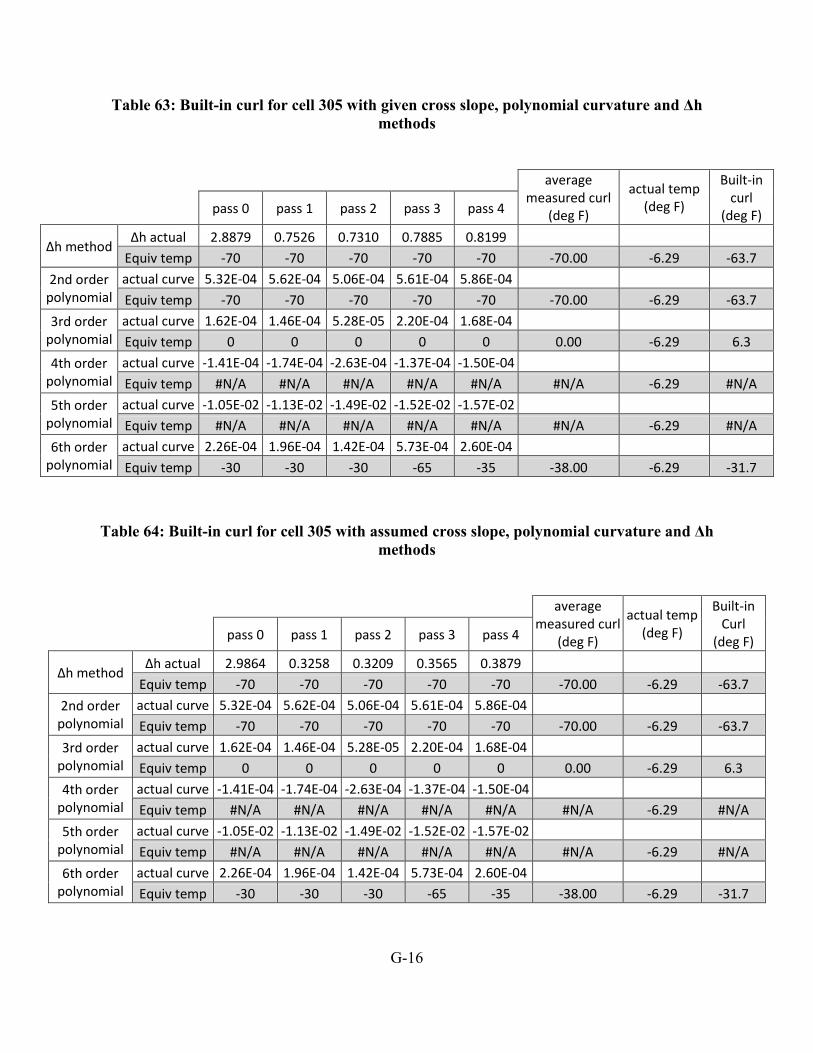
G-16
Table 63: Built-in curl for cell 305 with given cross slope, polynomial curvature and Δh methods
average
measured curl (deg F)
actual temp (deg F)
Built-in curl
(deg F)
pass 0 pass 1 pass 2 pass 3 pass 4
Δh method Δh actual 2.8879 0.7526 0.7310 0.7885 0.8199
Equiv temp -70 -70 -70 -70 -70 -70.00 -6.29 -63.7
2nd order polynomial
actual curve 5.32E-04 5.62E-04 5.06E-04 5.61E-04 5.86E-04 Equiv temp -70 -70 -70 -70 -70 -70.00 -6.29 -63.7
3rd order polynomial
actual curve 1.62E-04 1.46E-04 5.28E-05 2.20E-04 1.68E-04 Equiv temp 0 0 0 0 0 0.00 -6.29 6.3
4th order polynomial
actual curve -1.41E-04 -1.74E-04 -2.63E-04 -1.37E-04 -1.50E-04 Equiv temp #N/A #N/A #N/A #N/A #N/A #N/A -6.29 #N/A
5th order polynomial
actual curve -1.05E-02 -1.13E-02 -1.49E-02 -1.52E-02 -1.57E-02 Equiv temp #N/A #N/A #N/A #N/A #N/A #N/A -6.29 #N/A
6th order polynomial
actual curve 2.26E-04 1.96E-04 1.42E-04 5.73E-04 2.60E-04 Equiv temp -30 -30 -30 -65 -35 -38.00 -6.29 -31.7
Table 64: Built-in curl for cell 305 with assumed cross slope, polynomial curvature and Δh methods
average
measured curl (deg F)
actual temp (deg F)
Built-in Curl
(deg F)
pass 0 pass 1 pass 2 pass 3 pass 4
Δh method Δh actual 2.9864 0.3258 0.3209 0.3565 0.3879
Equiv temp -70 -70 -70 -70 -70 -70.00 -6.29 -63.7
2nd order polynomial
actual curve 5.32E-04 5.62E-04 5.06E-04 5.61E-04 5.86E-04 Equiv temp -70 -70 -70 -70 -70 -70.00 -6.29 -63.7
3rd order polynomial
actual curve 1.62E-04 1.46E-04 5.28E-05 2.20E-04 1.68E-04 Equiv temp 0 0 0 0 0 0.00 -6.29 6.3
4th order polynomial
actual curve -1.41E-04 -1.74E-04 -2.63E-04 -1.37E-04 -1.50E-04 Equiv temp #N/A #N/A #N/A #N/A #N/A #N/A -6.29 #N/A
5th order polynomial
actual curve -1.05E-02 -1.13E-02 -1.49E-02 -1.52E-02 -1.57E-02 Equiv temp #N/A #N/A #N/A #N/A #N/A #N/A -6.29 #N/A
6th order polynomial
actual curve 2.26E-04 1.96E-04 1.42E-04 5.73E-04 2.60E-04 Equiv temp -30 -30 -30 -65 -35 -38.00 -6.29 -31.7

G-17
Table 65: Built-in curl for cell 513 with given cross slope, polynomial curvature and Δh methods
average
measured curl (deg F)
actual temp (deg F)
Built-in curl
(deg F)
pass 0 pass 1 pass 2 pass 3 pass 4
Δh method Δh actual 2.9500 0.4209 0.4927 0.4806 0.4713
Equiv temp -70 -70 -70 -70 -70 -70.00 -3.78 -66.2
2nd order polynomial
actual curve 4.34E-04 3.04E-04 3.77E-04 3.49E-04 4.10E-04 Equiv temp -70 -70 -70 -70 -70 -70.00 -3.78 -66.2
3rd order polynomial
actual curve 4.35E-05 1.12E-04 1.82E-05 1.61E-04 1.14E-04 Equiv temp 0 0 0 0 0 0.00 -3.78 3.8
4th order polynomial
actual curve 2.34E-05 6.67E-05 -5.61E-05 1.11E-04 5.91E-05 Equiv temp -5 -15 15 -20 -10 -7.00 -3.78 -3.2
5th order polynomial
actual curve -1.22E-02 -2.67E-02 -2.87E-02 -2.54E-02 -3.32E-02 Equiv temp #N/A #N/A #N/A #N/A #N/A #N/A -3.78 #N/A
6th order polynomial
actual curve 2.04E-03 2.00E-03 1.81E-03 2.09E-03 2.38E-03 Equiv temp -70 -70 -70 -70 -70 -70.00 -3.78 -66.2
Table 66: built-in curl for cell 513 with assumed cross slope, polynomial curvature and Δh methods
average
measured curl (deg F)
actual temp (deg F)
Built-in curl
(deg F)
pass 0 pass 1 pass 2 pass 3 pass 4
Δh method Δh actual 2.9500 0.1453 0.1847 0.2083 0.2215
Equiv temp -70 -70 -70 -70 -70 -70.00 -3.78 -66.2
2nd order polynomial
actual curve 4.34E-04 3.04E-04 3.77E-04 3.49E-04 4.10E-04 Equiv temp -70 -70 -70 -70 -70 -70.00 -3.78 -66.2
3rd order polynomial
actual curve 4.35E-05 1.12E-04 1.82E-05 1.61E-04 1.14E-04 Equiv temp 0 0 0 0 0 0.00 -3.78 3.8
4th order polynomial
actual curve 2.34E-05 6.67E-05 -5.61E-05 1.11E-04 5.91E-05 Equiv temp -5 -15 15 -20 -10 -7.00 -3.78 -3.2
5th order polynomial
actual curve -1.22E-02 -2.67E-02 -2.87E-02 -2.54E-02 -3.32E-02 Equiv temp #N/A #N/A #N/A #N/A #N/A #N/A -3.78 #N/A
6th order polynomial
actual curve 2.04E-03 2.00E-03 1.81E-03 2.09E-03 2.38E-03 Equiv temp -70 -70 -70 -70 -70 -70.00 -3.78 -66.2

G-18
Table 67: Built-in curl for cell 614 with given cross slope, polynomial curvature and Δh methods
average
measured curl (deg F)
actual temp (deg F)
Built-in curl
(deg F)
pass 0 pass 1 pass 2 pass 3 pass 4
Δh method Δh actual 2.9021 0.2543 0.2274 0.2769 0.2381
Equiv temp -70 -70 -70 -65 -70 -69.00 -3.78 -65.2
2nd order polynomial
actual curve 3.47E-04 3.17E-04 3.07E-04 4.15E-04 -5.71E-05 Equiv temp -70 -70 -70 -65 25 -50.00 -3.78 -46.2
3rd order polynomial
actual curve 1.30E-04 -2.98E-04 -2.66E-04 -1.87E-04 -3.95E-04 Equiv temp -15 -5 -5 -5 -5 -7.00 -3.78 -3.2
4th order polynomial
actual curve 1.23E-04 -2.44E-04 -1.64E-04 -1.77E-04 1.35E-04 Equiv temp -40 #N/A #N/A #N/A -40 #N/A -3.78 #N/A
5th order polynomial
actual curve 3.09E-03 -1.85E-02 -1.92E-02 -2.41E-02 -9.92E-02 Equiv temp -70 #N/A #N/A #N/A #N/A #N/A -3.78 #N/A
6th order polynomial
actual curve 2.77E-03 1.73E-03 1.90E-03 2.66E-03 -3.59E-03 Equiv temp -70 -70 -70 -70 #N/A #N/A -3.78 #N/A
Table 68: Built-in curl for cell 614 with assumed cross slope, polynomial curvature and Δh methods
average
measured curl (deg F)
actual temp (deg F)
Built-in curl
(deg F)
pass 0 pass 1 pass 2 pass 3 pass 4
Δh method Δh actual 2.6321 0.1163 0.2162 0.1473 0.1001
Equiv temp -70 -70 -70 -65 -70 -69.00 -3.78 -65.2
2nd order polynomial
actual curve 3.47E-04 3.17E-04 3.07E-04 4.15E-04 7.73E-05 Equiv temp -70 -70 -70 -65 -45 -64.00 -3.78 -60.2
3rd order polynomial
actual curve 1.30E-04 -2.98E-04 -2.66E-04 -1.87E-04 2.47E-04 Equiv temp -15 -5 -5 -5 -15 -9.00 -3.78 -5.2
4th order polynomial
actual curve 1.23E-04 -2.44E-04 -1.64E-04 -1.77E-04 3.99E-04 Equiv temp -40 #N/A #N/A #N/A -70 #N/A -3.78 #N/A
5th order polynomial
actual curve 3.09E-03 -1.85E-02 -1.92E-02 -2.41E-02 -3.53E-02 Equiv temp -70 #N/A #N/A #N/A #N/A #N/A -3.78 #N/A
6th order polynomial
actual curve 2.77E-03 1.73E-03 1.90E-03 2.66E-03 2.77E-03 Equiv temp -70 -70 -70 -70 -70 -70.00 -3.78 -66.2

APPENDIX H: BUILT-IN CURL AS DETERMINED FROM THE PROFILOMETER USING VARIOUS BEST FIT METHODS – HALF
SLABS

H-1
Table 69: Built-in curl for cell 7, polynomial curvature method for half slabs
average
measured curl (deg F)
actual temp (deg F)
Built-in curl
(deg F)
pass 0 pass 1 pass 2 pass 3 pass 4
Δh method Δh actual 3.1699 0.1681 0.0912 0.1170 0.1441
Equiv temp -70 -70 -70 -70 -70 -70.00 -6.79 -63.2
2nd order polynomial
actual curve 5.60E-04 5.32E-04 3.61E-04 4.28E-04 2.93E-04 Equiv temp -70 -70 -70 -70 -70 -70.00 -6.79 -63.2
3rd order polynomial
actual curve -4.20E-04 4.83E-05 -4.82E-04 -4.46E-04 -7.28E-05 Equiv temp 5 0 5 5 5 4.00 -6.79 10.8
4th order polynomial
actual curve -1.36E-03 -1.01E-04 -5.08E-04 -3.54E-04 -2.52E-04 Equiv temp #N/A #N/A #N/A #N/A #N/A #N/A -6.79 #N/A
5th order polynomial
actual curve 3.27E-02 2.63E-02 2.69E-02 -3.53E-03 1.24E-02 Equiv temp -70 -70 -70 #N/A -70 #N/A -6.79 #N/A
6th order polynomial
actual curve -1.19E-03 5.71E-04 4.96E-04 -2.06E-04 2.52E-04 Equiv temp #N/A -70 -70 #N/A -45 #N/A -6.79 #N/A
Table 70: Built-in curl for cell 12, polynomial curvature method for half slabs
average
measured curl (deg F)
actual temp (deg F)
Built-in curl
(deg F)
pass 0 pass 1 pass 2 pass 3 pass 4
Δh method Δh actual 2.9443 0.1471 0.1104 0.1197 0.0276
Equiv temp -70 -70 -70 0 -70 -56.00 -10.93 -45.1
2nd order polynomial
actual curve 4.81E-04 4.65E-04 3.18E-04 3.67E-04 3.49E-04 Equiv temp -70 -70 -70 -70 -70 -70.00 -10.93 -59.1
3rd order polynomial
actual curve -6.18E-05 9.73E-05 -1.76E-04 -6.25E-04 -7.82E-04 Equiv temp 5 0 5 10 10 6.00 -10.93 16.9
4th order polynomial
actual curve -9.69E-04 -8.69E-04 -8.57E-04 -1.33E-03 -7.60E-04 Equiv temp #N/A #N/A #N/A #N/A #N/A #N/A -10.93 #N/A
5th order polynomial
actual curve 4.29E-02 7.26E-02 6.34E-02 6.95E-02 2.43E-03 Equiv temp -70 -70 -70 -70 -70 -70.00 -10.93 -59.1
6th order polynomial
actual curve -1.83E-03 -8.73E-04 -5.71E-04 -7.20E-04 -1.25E-03 Equiv temp #N/A #N/A #N/A #N/A #N/A #N/A -10.93 #N/A
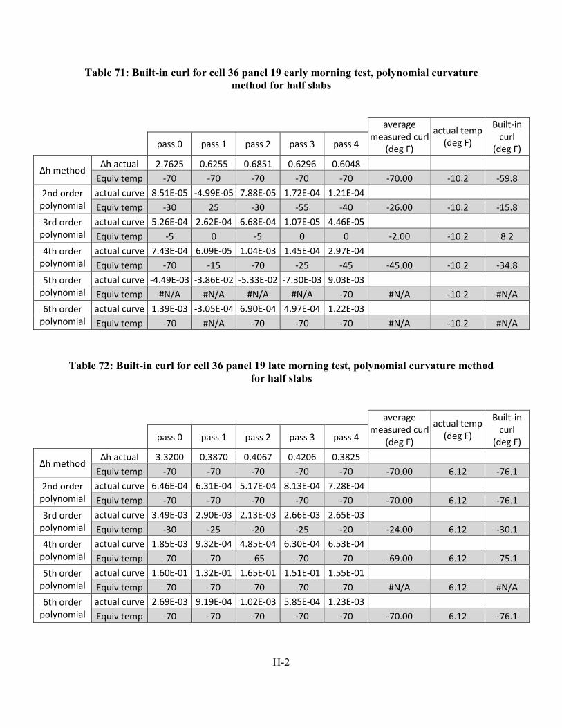
H-2
Table 71: Built-in curl for cell 36 panel 19 early morning test, polynomial curvature method for half slabs
average
measured curl (deg F)
actual temp (deg F)
Built-in curl
(deg F) pass 0 pass 1 pass 2 pass 3 pass 4
Δh method Δh actual 2.7625 0.6255 0.6851 0.6296 0.6048
Equiv temp -70 -70 -70 -70 -70 -70.00 -10.2 -59.8
2nd order polynomial
actual curve 8.51E-05 -4.99E-05 7.88E-05 1.72E-04 1.21E-04 Equiv temp -30 25 -30 -55 -40 -26.00 -10.2 -15.8
3rd order polynomial
actual curve 5.26E-04 2.62E-04 6.68E-04 1.07E-05 4.46E-05 Equiv temp -5 0 -5 0 0 -2.00 -10.2 8.2
4th order polynomial
actual curve 7.43E-04 6.09E-05 1.04E-03 1.45E-04 2.97E-04 Equiv temp -70 -15 -70 -25 -45 -45.00 -10.2 -34.8
5th order polynomial
actual curve -4.49E-03 -3.86E-02 -5.33E-02 -7.30E-03 9.03E-03 Equiv temp #N/A #N/A #N/A #N/A -70 #N/A -10.2 #N/A
6th order polynomial
actual curve 1.39E-03 -3.05E-04 6.90E-04 4.97E-04 1.22E-03 Equiv temp -70 #N/A -70 -70 -70 #N/A -10.2 #N/A
Table 72: Built-in curl for cell 36 panel 19 late morning test, polynomial curvature method for half slabs
average
measured curl (deg F)
actual temp (deg F)
Built-in curl
(deg F) pass 0 pass 1 pass 2 pass 3 pass 4
Δh method Δh actual 3.3200 0.3870 0.4067 0.4206 0.3825
Equiv temp -70 -70 -70 -70 -70 -70.00 6.12 -76.1
2nd order polynomial
actual curve 6.46E-04 6.31E-04 5.17E-04 8.13E-04 7.28E-04 Equiv temp -70 -70 -70 -70 -70 -70.00 6.12 -76.1
3rd order polynomial
actual curve 3.49E-03 2.90E-03 2.13E-03 2.66E-03 2.65E-03 Equiv temp -30 -25 -20 -25 -20 -24.00 6.12 -30.1
4th order polynomial
actual curve 1.85E-03 9.32E-04 4.85E-04 6.30E-04 6.53E-04 Equiv temp -70 -70 -65 -70 -70 -69.00 6.12 -75.1
5th order polynomial
actual curve 1.60E-01 1.32E-01 1.65E-01 1.51E-01 1.55E-01 Equiv temp -70 -70 -70 -70 -70 #N/A 6.12 #N/A
6th order polynomial
actual curve 2.69E-03 9.19E-04 1.02E-03 5.85E-04 1.23E-03 Equiv temp -70 -70 -70 -70 -70 -70.00 6.12 -76.1
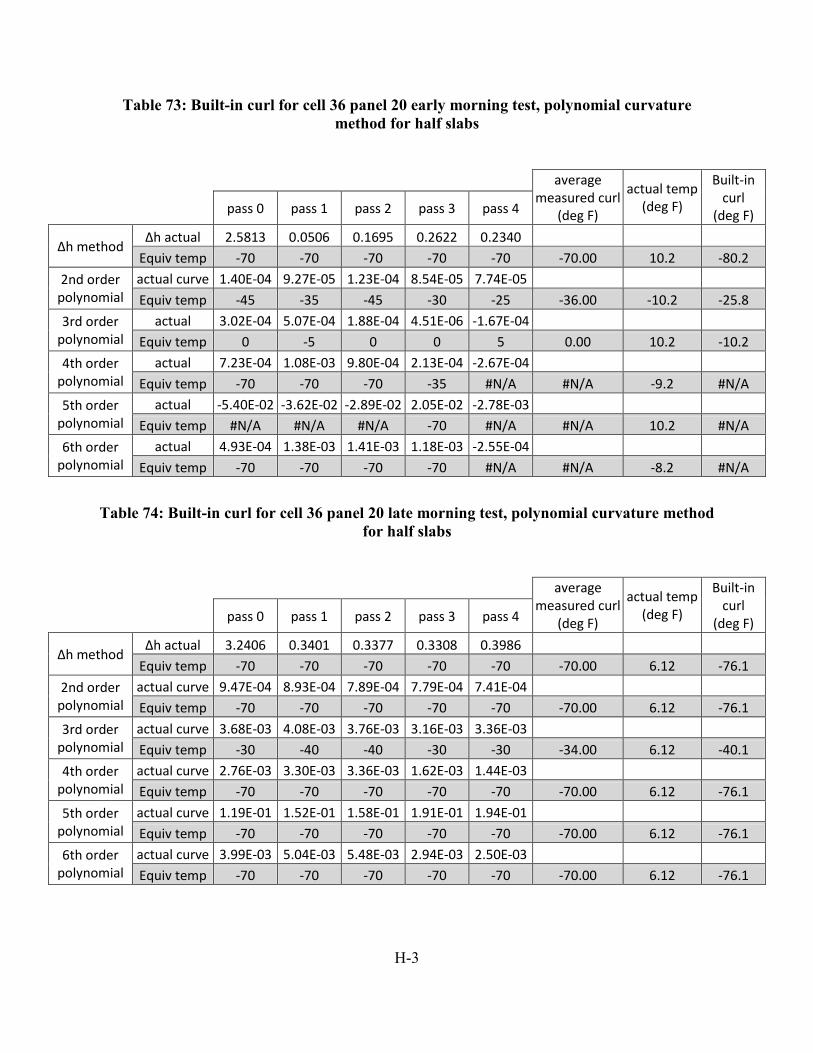
H-3
Table 73: Built-in curl for cell 36 panel 20 early morning test, polynomial curvature method for half slabs
average
measured curl (deg F)
actual temp (deg F)
Built-in curl
(deg F) pass 0 pass 1 pass 2 pass 3 pass 4
Δh method Δh actual 2.5813 0.0506 0.1695 0.2622 0.2340
Equiv temp -70 -70 -70 -70 -70 -70.00 10.2 -80.2
2nd order polynomial
actual curve 1.40E-04 9.27E-05 1.23E-04 8.54E-05 7.74E-05 Equiv temp -45 -35 -45 -30 -25 -36.00 -10.2 -25.8
3rd order polynomial
actual 3.02E-04 5.07E-04 1.88E-04 4.51E-06 -1.67E-04 Equiv temp 0 -5 0 0 5 0.00 10.2 -10.2
4th order polynomial
actual 7.23E-04 1.08E-03 9.80E-04 2.13E-04 -2.67E-04 Equiv temp -70 -70 -70 -35 #N/A #N/A -9.2 #N/A
5th order polynomial
actual -5.40E-02 -3.62E-02 -2.89E-02 2.05E-02 -2.78E-03 Equiv temp #N/A #N/A #N/A -70 #N/A #N/A 10.2 #N/A
6th order polynomial
actual 4.93E-04 1.38E-03 1.41E-03 1.18E-03 -2.55E-04 Equiv temp -70 -70 -70 -70 #N/A #N/A -8.2 #N/A
Table 74: Built-in curl for cell 36 panel 20 late morning test, polynomial curvature method for half slabs
average
measured curl (deg F)
actual temp (deg F)
Built-in curl
(deg F) pass 0 pass 1 pass 2 pass 3 pass 4
Δh method Δh actual 3.2406 0.3401 0.3377 0.3308 0.3986
Equiv temp -70 -70 -70 -70 -70 -70.00 6.12 -76.1
2nd order polynomial
actual curve 9.47E-04 8.93E-04 7.89E-04 7.79E-04 7.41E-04 Equiv temp -70 -70 -70 -70 -70 -70.00 6.12 -76.1
3rd order polynomial
actual curve 3.68E-03 4.08E-03 3.76E-03 3.16E-03 3.36E-03 Equiv temp -30 -40 -40 -30 -30 -34.00 6.12 -40.1
4th order polynomial
actual curve 2.76E-03 3.30E-03 3.36E-03 1.62E-03 1.44E-03 Equiv temp -70 -70 -70 -70 -70 -70.00 6.12 -76.1
5th order polynomial
actual curve 1.19E-01 1.52E-01 1.58E-01 1.91E-01 1.94E-01 Equiv temp -70 -70 -70 -70 -70 -70.00 6.12 -76.1
6th order polynomial
actual curve 3.99E-03 5.04E-03 5.48E-03 2.94E-03 2.50E-03 Equiv temp -70 -70 -70 -70 -70 -70.00 6.12 -76.1

H-4
Table 75: Built-in curl for cell 37 panel 8 early morning test, polynomial curvature method for half slabs
average
measured curl (deg F)
actual temp (deg F)
Built-in curl
(deg F) pass 0 pass 1 pass 2 pass 3 pass 4
Δh method Δh actual 2.6415 0.4449 0.2334 0.4482 0.3673
Equiv temp -70 -70 -70 -70 -70 -70.00 -10.43 -59.6
2nd order polynomial
actual curve 2.31E-05 -2.45E-05 -2.77E-06 -1.02E-04 5.46E-05 Equiv temp -10 15 5 #N/A -20 #N/A -10.43 #N/A
3rd order polynomial
actual curve -5.23E-04 -3.48E-04 -2.68E-04 -3.75E-04 -3.84E-04 Equiv temp 5 5 5 5 5 5.00 -10.43 15.4
4th order polynomial
actual curve 4.76E-05 1.08E-05 1.89E-04 5.68E-04 -1.25E-04 Equiv temp -10 0 -35 -70 30 -17.00 -10.43 -6.6
5th order polynomial
actual curve -2.30E-02 -3.48E-02 -3.88E-02 -7.15E-02 -2.47E-02 Equiv temp #N/A #N/A #N/A #N/A #N/A #N/A -10.43 #N/A
6th order polynomial
actual curve 7.57E-04 3.55E-04 5.02E-04 5.38E-04 1.11E-04 Equiv temp -70 -50 -70 -70 -20 -56.00 -10.43 -45.6
Table 76: Built-in curl for cell 37 panel 8 late morning test, polynomial curvature method for half slabs
average
measured curl (deg F)
actual temp (deg F)
Built-in curl
(deg F) pass 0 pass 1 pass 2 pass 3 pass 4
Δh method Δh actual 3.4791 0.3548 0.1028 0.3922 0.1100
Equiv temp -70 -70 -70 -70 -70 -70.00 9.75 -79.8
2nd order polynomial
actual curve 5.09E-04 5.55E-04 5.27E-04 4.19E-04 4.61E-04 Equiv temp -70 -70 -70 30 -70 -50.00 9.75 -59.8
3rd order polynomial
actual curve 2.01E-03 2.33E-03 2.39E-03 2.50E-03 2.43E-03 Equiv temp -15 -20 -20 -20 -20 -19.00 9.75 -28.8
4th order polynomial
actual curve -1.67E-04 2.17E-04 1.21E-04 7.43E-04 5.42E-04 Equiv temp #N/A -35 -25 -70 -70 #N/A 9.75 #N/A
5th order polynomial
actual curve 2.70E-02 1.73E-02 8.77E-03 -4.10E-02 -1.68E-02 Equiv temp -70 -70 -70 #N/A #N/A #N/A 9.75 #N/A
6th order polynomial
actual curve -2.90E-03 -2.67E-03 -3.22E-03 -3.09E-03 -3.01E-03 Equiv temp #N/A #N/A #N/A #N/A #N/A #N/A 9.75 #N/A
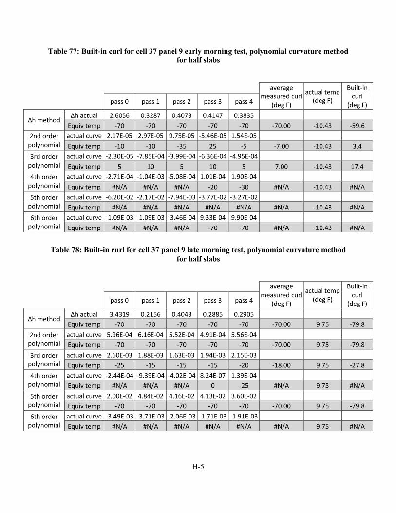
H-5
Table 77: Built-in curl for cell 37 panel 9 early morning test, polynomial curvature method for half slabs
average
measured curl (deg F)
actual temp (deg F)
Built-in curl
(deg F) pass 0 pass 1 pass 2 pass 3 pass 4
Δh method Δh actual 2.6056 0.3287 0.4073 0.4147 0.3835
Equiv temp -70 -70 -70 -70 -70 -70.00 -10.43 -59.6
2nd order polynomial
actual curve 2.17E-05 2.97E-05 9.75E-05 -5.46E-05 1.54E-05 Equiv temp -10 -10 -35 25 -5 -7.00 -10.43 3.4
3rd order polynomial
actual curve -2.30E-05 -7.85E-04 -3.99E-04 -6.36E-04 -4.95E-04 Equiv temp 5 10 5 10 5 7.00 -10.43 17.4
4th order polynomial
actual curve -2.71E-04 -1.04E-03 -5.08E-04 1.01E-04 1.90E-04 Equiv temp #N/A #N/A #N/A -20 -30 #N/A -10.43 #N/A
5th order polynomial
actual curve -6.20E-02 -2.17E-02 -7.94E-03 -3.77E-02 -3.27E-02 Equiv temp #N/A #N/A #N/A #N/A #N/A #N/A -10.43 #N/A
6th order polynomial
actual curve -1.09E-03 -1.09E-03 -3.46E-04 9.33E-04 9.90E-04 Equiv temp #N/A #N/A #N/A -70 -70 #N/A -10.43 #N/A
Table 78: Built-in curl for cell 37 panel 9 late morning test, polynomial curvature method for half slabs
average
measured curl (deg F)
actual temp (deg F)
Built-in curl
(deg F) pass 0 pass 1 pass 2 pass 3 pass 4
Δh method Δh actual 3.4319 0.2156 0.4043 0.2885 0.2905
Equiv temp -70 -70 -70 -70 -70 -70.00 9.75 -79.8
2nd order polynomial
actual curve 5.96E-04 6.16E-04 5.52E-04 4.91E-04 5.56E-04 Equiv temp -70 -70 -70 -70 -70 -70.00 9.75 -79.8
3rd order polynomial
actual curve 2.60E-03 1.88E-03 1.63E-03 1.94E-03 2.15E-03 Equiv temp -25 -15 -15 -15 -20 -18.00 9.75 -27.8
4th order polynomial
actual curve -2.44E-04 -9.39E-04 -4.02E-04 8.24E-07 1.39E-04 Equiv temp #N/A #N/A #N/A 0 -25 #N/A 9.75 #N/A
5th order polynomial
actual curve 2.00E-02 4.84E-02 4.16E-02 4.13E-02 3.60E-02 Equiv temp -70 -70 -70 -70 -70 -70.00 9.75 -79.8
6th order polynomial
actual curve -3.49E-03 -3.71E-03 -2.06E-03 -1.71E-03 -1.91E-03 Equiv temp #N/A #N/A #N/A #N/A #N/A #N/A 9.75 #N/A
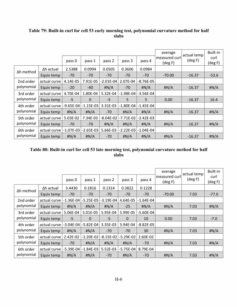
H-6
Table 79: Built-in curl for cell 53 early morning test, polynomial curvature method for half slabs
average
measured curl (deg F)
actual temp (deg F)
Built-in curl
(deg F) pass 0 pass 1 pass 2 pass 3 pass 4
Δh method Δh actual 2.5388 0.0994 0.0505 0.3606 0.0984
Equiv temp -70 -70 -70 -70 -70 -70.00 -16.37 -53.6
2nd order polynomial
actual curve 4.14E-05 7.91E-05 -2.01E-04 2.07E-04 -8.76E-05 Equiv temp -20 -40 #N/A -70 #N/A #N/A -16.37 #N/A
3rd order polynomial
actual curve 4.70E-04 1.80E-04 5.32E-04 -1.98E-04 -3.56E-04 Equiv temp -5 0 -5 5 5 0.00 -16.37 16.4
4th order polynomial
actual curve -9.65E-04 -1.15E-03 3.31E-03 -1.80E-04 -1.45E-04 Equiv temp #N/A #N/A -70 #N/A #N/A #N/A -16.37 #N/A
5th order polynomial
actual curve 5.03E-02 7.34E-03 -8.04E-02 -7.71E-02 -2.42E-03 Equiv temp -70 -70 #N/A #N/A #N/A #N/A -16.37 #N/A
6th order polynomial
actual curve -1.07E-03 -2.65E-03 5.66E-03 -2.22E-03 -1.04E-04 Equiv temp #N/A #N/A -70 #N/A #N/A #N/A -16.37 #N/A
Table 80: Built-in curl for cell 53 late morning test, polynomial curvature method for half slabs
average
measured curl (deg F)
actual temp (deg F)
Built-in curl
(deg F) pass 0 pass 1 pass 2 pass 3 pass 4
Δh method Δh actual 3.4430 0.1816 0.1314 0.3822 0.1228
Equiv temp -70 -70 -70 -70 -70 -70.00 7.03 -77.0
2nd order polynomial
actual curve -1.36E-04 -5.25E-05 -3.19E-04 4.64E-05 -1.64E-04 Equiv temp #N/A #N/A #N/A -25 #N/A #N/A 7.03 #N/A
3rd order polynomial
actual curve 5.06E-04 5.01E-05 5.95E-04 5.99E-05 -5.60E-04 Equiv temp -5 0 -5 0 10 0.00 7.03 -7.0
4th order polynomial
actual curve -3.04E-04 -5.82E-04 3.35E-03 3.94E-04 -8.82E-05 Equiv temp #N/A #N/A -70 -70 30 #N/A 7.03 #N/A
5th order polynomial
actual curve 2.42E-02 -2.20E-02 -8.15E-02 -5.29E-02 2.60E-02 Equiv temp -70 #N/A #N/A #N/A -70 #N/A 7.03 #N/A
6th order polynomial
actual curve -5.39E-04 -1.84E-03 5.52E-03 -5.75E-04 8.79E-04 Equiv temp #N/A #N/A -70 #N/A -70 #N/A 7.03 #N/A
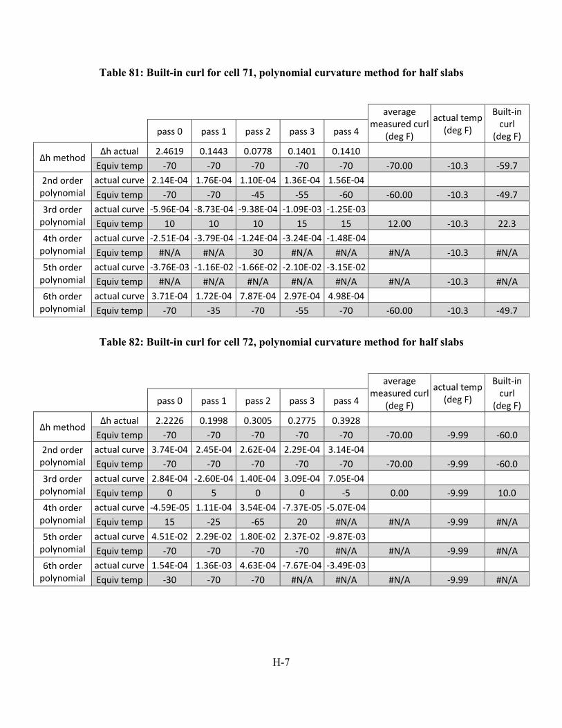
H-7
Table 81: Built-in curl for cell 71, polynomial curvature method for half slabs
average
measured curl (deg F)
actual temp (deg F)
Built-in curl
(deg F) pass 0 pass 1 pass 2 pass 3 pass 4
Δh method Δh actual 2.4619 0.1443 0.0778 0.1401 0.1410
Equiv temp -70 -70 -70 -70 -70 -70.00 -10.3 -59.7
2nd order polynomial
actual curve 2.14E-04 1.76E-04 1.10E-04 1.36E-04 1.56E-04 Equiv temp -70 -70 -45 -55 -60 -60.00 -10.3 -49.7
3rd order polynomial
actual curve -5.96E-04 -8.73E-04 -9.38E-04 -1.09E-03 -1.25E-03 Equiv temp 10 10 10 15 15 12.00 -10.3 22.3
4th order polynomial
actual curve -2.51E-04 -3.79E-04 -1.24E-04 -3.24E-04 -1.48E-04 Equiv temp #N/A #N/A 30 #N/A #N/A #N/A -10.3 #N/A
5th order polynomial
actual curve -3.76E-03 -1.16E-02 -1.66E-02 -2.10E-02 -3.15E-02 Equiv temp #N/A #N/A #N/A #N/A #N/A #N/A -10.3 #N/A
6th order polynomial
actual curve 3.71E-04 1.72E-04 7.87E-04 2.97E-04 4.98E-04 Equiv temp -70 -35 -70 -55 -70 -60.00 -10.3 -49.7
Table 82: Built-in curl for cell 72, polynomial curvature method for half slabs
average
measured curl (deg F)
actual temp (deg F)
Built-in curl
(deg F) pass 0 pass 1 pass 2 pass 3 pass 4
Δh method Δh actual 2.2226 0.1998 0.3005 0.2775 0.3928
Equiv temp -70 -70 -70 -70 -70 -70.00 -9.99 -60.0
2nd order polynomial
actual curve 3.74E-04 2.45E-04 2.62E-04 2.29E-04 3.14E-04 Equiv temp -70 -70 -70 -70 -70 -70.00 -9.99 -60.0
3rd order polynomial
actual curve 2.84E-04 -2.60E-04 1.40E-04 3.09E-04 7.05E-04 Equiv temp 0 5 0 0 -5 0.00 -9.99 10.0
4th order polynomial
actual curve -4.59E-05 1.11E-04 3.54E-04 -7.37E-05 -5.07E-04 Equiv temp 15 -25 -65 20 #N/A #N/A -9.99 #N/A
5th order polynomial
actual curve 4.51E-02 2.29E-02 1.80E-02 2.37E-02 -9.87E-03 Equiv temp -70 -70 -70 -70 #N/A #N/A -9.99 #N/A
6th order polynomial
actual curve 1.54E-04 1.36E-03 4.63E-04 -7.67E-04 -3.49E-03 Equiv temp -30 -70 -70 #N/A #N/A #N/A -9.99 #N/A
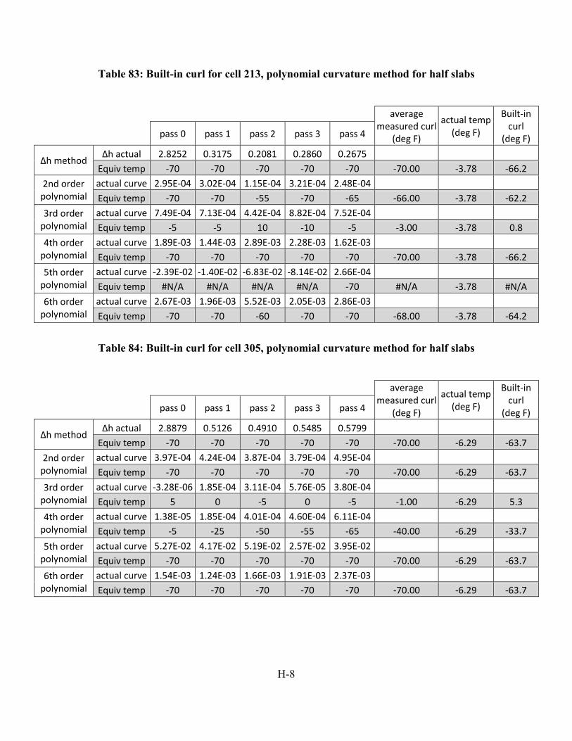
H-8
Table 83: Built-in curl for cell 213, polynomial curvature method for half slabs
average
measured curl (deg F)
actual temp (deg F)
Built-in curl
(deg F) pass 0 pass 1 pass 2 pass 3 pass 4
Δh method Δh actual 2.8252 0.3175 0.2081 0.2860 0.2675
Equiv temp -70 -70 -70 -70 -70 -70.00 -3.78 -66.2
2nd order polynomial
actual curve 2.95E-04 3.02E-04 1.15E-04 3.21E-04 2.48E-04 Equiv temp -70 -70 -55 -70 -65 -66.00 -3.78 -62.2
3rd order polynomial
actual curve 7.49E-04 7.13E-04 4.42E-04 8.82E-04 7.52E-04 Equiv temp -5 -5 10 -10 -5 -3.00 -3.78 0.8
4th order polynomial
actual curve 1.89E-03 1.44E-03 2.89E-03 2.28E-03 1.62E-03 Equiv temp -70 -70 -70 -70 -70 -70.00 -3.78 -66.2
5th order polynomial
actual curve -2.39E-02 -1.40E-02 -6.83E-02 -8.14E-02 2.66E-04 Equiv temp #N/A #N/A #N/A #N/A -70 #N/A -3.78 #N/A
6th order polynomial
actual curve 2.67E-03 1.96E-03 5.52E-03 2.05E-03 2.86E-03 Equiv temp -70 -70 -60 -70 -70 -68.00 -3.78 -64.2
Table 84: Built-in curl for cell 305, polynomial curvature method for half slabs
average
measured curl (deg F)
actual temp (deg F)
Built-in curl
(deg F) pass 0 pass 1 pass 2 pass 3 pass 4
Δh method Δh actual 2.8879 0.5126 0.4910 0.5485 0.5799
Equiv temp -70 -70 -70 -70 -70 -70.00 -6.29 -63.7
2nd order polynomial
actual curve 3.97E-04 4.24E-04 3.87E-04 3.79E-04 4.95E-04 Equiv temp -70 -70 -70 -70 -70 -70.00 -6.29 -63.7
3rd order polynomial
actual curve -3.28E-06 1.85E-04 3.11E-04 5.76E-05 3.80E-04 Equiv temp 5 0 -5 0 -5 -1.00 -6.29 5.3
4th order polynomial
actual curve 1.38E-05 1.85E-04 4.01E-04 4.60E-04 6.11E-04 Equiv temp -5 -25 -50 -55 -65 -40.00 -6.29 -33.7
5th order polynomial
actual curve 5.27E-02 4.17E-02 5.19E-02 2.57E-02 3.95E-02 Equiv temp -70 -70 -70 -70 -70 -70.00 -6.29 -63.7
6th order polynomial
actual curve 1.54E-03 1.24E-03 1.66E-03 1.91E-03 2.37E-03 Equiv temp -70 -70 -70 -70 -70 -70.00 -6.29 -63.7
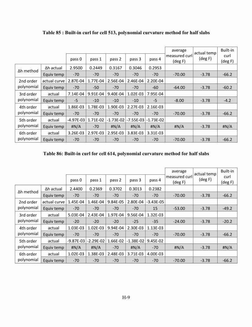
H-9
Table 85 : Built-in curl for cell 513, polynomial curvature method for half slabs
average
measured curl (deg F)
actual temp (deg F)
Built-in curl
(deg F) pass 0 pass 1 pass 2 pass 3 pass 4
Δh method Δh actual 2.9500 0.2449 0.3167 0.3046 0.2953
Equiv temp -70 -70 -70 -70 -70 -70.00 -3.78 -66.2
2nd order polynomial
actual curve 2.87E-04 1.77E-04 2.56E-04 2.46E-04 2.20E-04 Equiv temp -70 -50 -70 -70 -60 -64.00 -3.78 -60.2
3rd order polynomial
actual 7.14E-04 9.91E-04 9.40E-04 1.02E-03 7.95E-04 Equiv temp -5 -10 -10 -10 -5 -8.00 -3.78 -4.2
4th order polynomial
actual 1.86E-03 1.78E-03 1.90E-03 2.27E-03 2.16E-03 Equiv temp -70 -70 -70 -70 -70 -70.00 -3.78 -66.2
5th order polynomial
actual -4.97E-03 1.71E-02 -1.73E-02 -7.55E-03 -1.73E-02 Equiv temp #N/A -70 #N/A #N/A #N/A #N/A -3.78 #N/A
6th order polynomial
actual 3.26E-03 2.97E-03 2.95E-03 3.83E-03 3.31E-03 Equiv temp -70 -70 -70 -70 -70 -70.00 -3.78 -66.2
Table 86: Built-in curl for cell 614, polynomial curvature method for half slabs
average
measured curl (deg F)
actual temp (deg F)
Built-in curl
(deg F) pass 0 pass 1 pass 2 pass 3 pass 4
Δh method Δh actual 2.4400 0.2369 0.3702 0.3013 0.2382
Equiv temp -70 -70 -70 -70 -70 -70.00 -3.78 -66.2
2nd order polynomial
actual curve 1.45E-04 1.46E-04 9.84E-05 2.80E-04 -3.43E-05 Equiv temp -70 -70 -70 -70 15 -53.00 -3.78 -49.2
3rd order polynomial
actual 5.03E-04 2.43E-04 1.97E-04 9.56E-04 1.32E-03 Equiv temp -20 -20 -20 -25 -35 -24.00 -3.78 -20.2
4th order polynomial
actual 1.03E-03 1.02E-03 9.94E-04 2.30E-03 1.13E-03 Equiv temp -70 -70 -70 -70 -70 -70.00 -3.78 -66.2
5th order polynomial
actual -9.87E-03 -2.29E-02 1.66E-02 -1.38E-02 9.45E-02 Equiv temp #N/A #N/A -70 #N/A -70 #N/A -3.78 #N/A
6th order polynomial
actual 1.02E-03 1.38E-03 2.48E-03 3.71E-03 4.00E-03 Equiv temp -70 -70 -70 -70 -70 -70.00 -3.78 -66.2

APPENDIX I: BUILT-IN CURL AS DETERMINED FROM MINIMUM ERROR METHOD FOR FULL SLABS WITH ACTUAL DATA AND
POLYNOMIAL APPROXIMATIONS
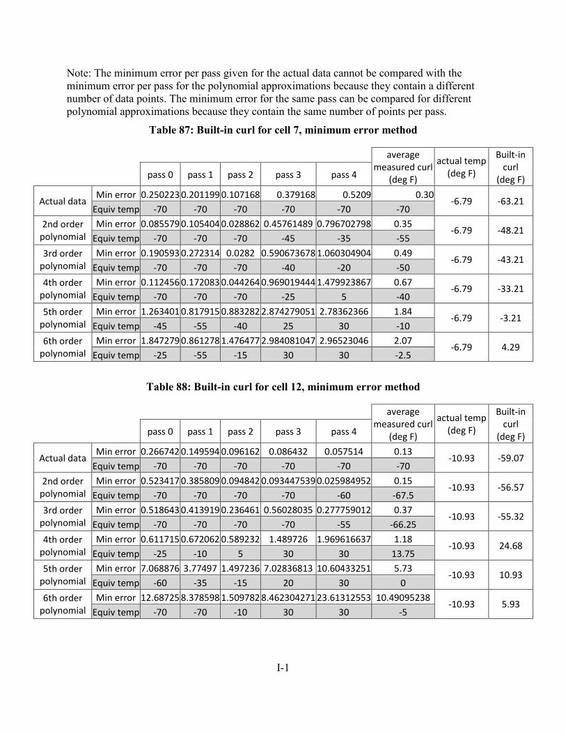
I-1
Note: The minimum error per pass given for the actual data cannot be compared with the minimum error per pass for the polynomial approximations because they contain a different number of data points. The minimum error for the same pass can be compared for different polynomial approximations because they contain the same number of points per pass.
Table 87: Built-in curl for cell 7, minimum error method
average
measured curl (deg F)
actual temp (deg F)
Built-in curl
(deg F) pass 0 pass 1 pass 2 pass 3 pass 4
Actual data Min error 0.250223 0.201199 0.107168 0.379168 0.5209 0.30
-6.79 -63.21 Equiv temp -70 -70 -70 -70 -70 -70
2nd order polynomial
Min error 0.085579 0.105404 0.028862 0.45761489 0.796702798 0.35 -6.79 -48.21
Equiv temp -70 -70 -70 -45 -35 -55
3rd order polynomial
Min error 0.190593 0.272314 0.0282 0.590673678 1.060304904 0.49 -6.79 -43.21
Equiv temp -70 -70 -70 -40 -20 -50
4th order polynomial
Min error 0.112456 0.172083 0.044264 0.969019444 1.479923867 0.67 -6.79 -33.21
Equiv temp -70 -70 -70 -25 5 -40
5th order polynomial
Min error 1.263401 0.817915 0.883282 2.874279051 2.78362366 1.84 -6.79 -3.21
Equiv temp -45 -55 -40 25 30 -10
6th order polynomial
Min error 1.847279 0.861278 1.476477 2.984081047 2.96523046 2.07 -6.79 4.29
Equiv temp -25 -55 -15 30 30 -2.5
Table 88: Built-in curl for cell 12, minimum error method
average
measured curl (deg F)
actual temp (deg F)
Built-in curl
(deg F) pass 0 pass 1 pass 2 pass 3 pass 4
Actual data Min error 0.266742 0.149594 0.096162 0.086432 0.057514 0.13
-10.93 -59.07 Equiv temp -70 -70 -70 -70 -70 -70
2nd order polynomial
Min error 0.523417 0.385809 0.094842 0.093447539 0.025984952 0.15 -10.93 -56.57
Equiv temp -70 -70 -70 -70 -60 -67.5
3rd order polynomial
Min error 0.518643 0.413919 0.236461 0.56028035 0.277759012 0.37 -10.93 -55.32
Equiv temp -70 -70 -70 -70 -55 -66.25
4th order polynomial
Min error 0.611715 0.672062 0.589232 1.489726 1.969616637 1.18 -10.93 24.68
Equiv temp -25 -10 5 30 30 13.75
5th order polynomial
Min error 7.068876 3.77497 1.497236 7.02836813 10.60433251 5.73 -10.93 10.93
Equiv temp -60 -35 -15 20 30 0
6th order polynomial
Min error 12.68725 8.378598 1.509782 8.462304271 23.61312553 10.49095238 -10.93 5.93
Equiv temp -70 -70 -10 30 30 -5
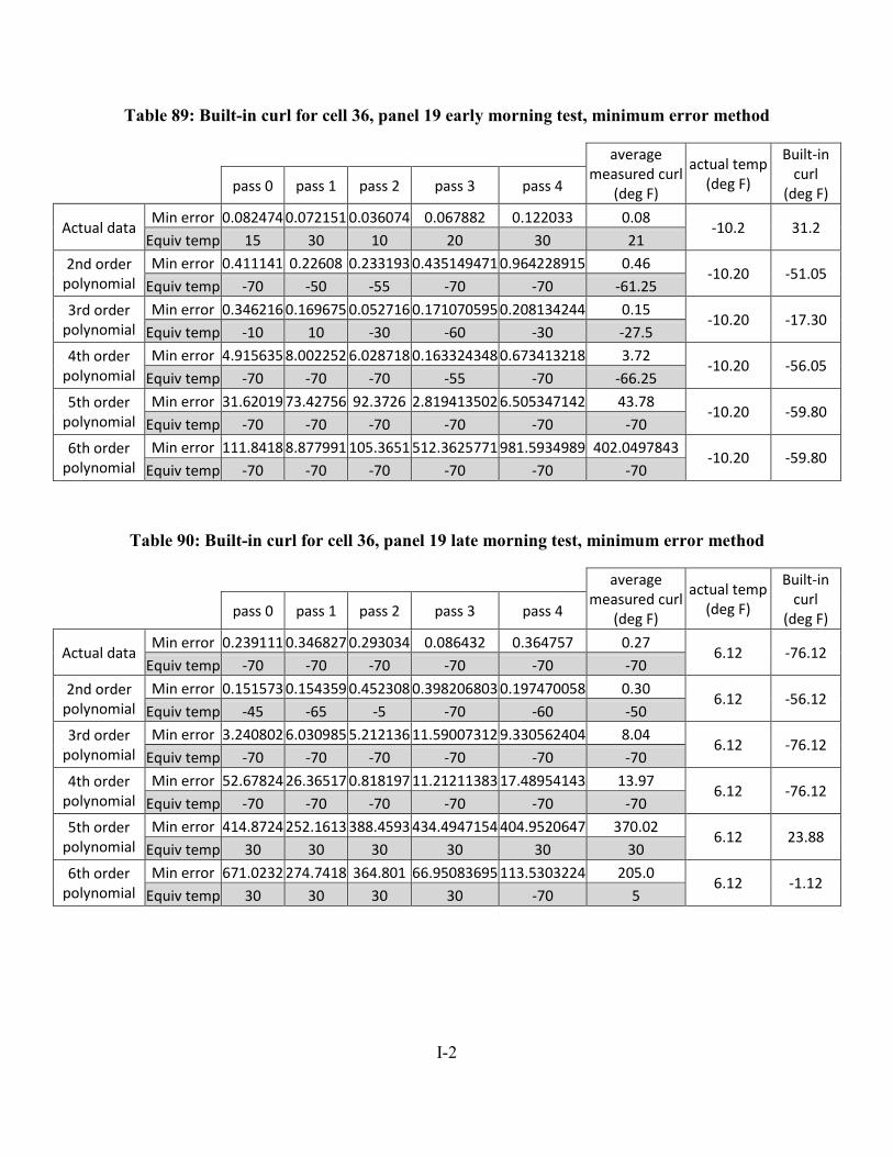
I-2
Table 89: Built-in curl for cell 36, panel 19 early morning test, minimum error method
average
measured curl (deg F)
actual temp (deg F)
Built-in curl
(deg F) pass 0 pass 1 pass 2 pass 3 pass 4
Actual data Min error 0.082474 0.072151 0.036074 0.067882 0.122033 0.08
-10.2 31.2 Equiv temp 15 30 10 20 30 21
2nd order polynomial
Min error 0.411141 0.22608 0.233193 0.435149471 0.964228915 0.46 -10.20 -51.05
Equiv temp -70 -50 -55 -70 -70 -61.25
3rd order polynomial
Min error 0.346216 0.169675 0.052716 0.171070595 0.208134244 0.15 -10.20 -17.30
Equiv temp -10 10 -30 -60 -30 -27.5
4th order polynomial
Min error 4.915635 8.002252 6.028718 0.163324348 0.673413218 3.72 -10.20 -56.05
Equiv temp -70 -70 -70 -55 -70 -66.25
5th order polynomial
Min error 31.62019 73.42756 92.3726 2.819413502 6.505347142 43.78 -10.20 -59.80
Equiv temp -70 -70 -70 -70 -70 -70
6th order polynomial
Min error 111.8418 8.877991 105.3651 512.3625771 981.5934989 402.0497843 -10.20 -59.80
Equiv temp -70 -70 -70 -70 -70 -70
Table 90: Built-in curl for cell 36, panel 19 late morning test, minimum error method
average
measured curl (deg F)
actual temp (deg F)
Built-in curl
(deg F) pass 0 pass 1 pass 2 pass 3 pass 4
Actual data Min error 0.239111 0.346827 0.293034 0.086432 0.364757 0.27
6.12 -76.12 Equiv temp -70 -70 -70 -70 -70 -70
2nd order polynomial
Min error 0.151573 0.154359 0.452308 0.398206803 0.197470058 0.30 6.12 -56.12
Equiv temp -45 -65 -5 -70 -60 -50
3rd order polynomial
Min error 3.240802 6.030985 5.212136 11.59007312 9.330562404 8.04 6.12 -76.12
Equiv temp -70 -70 -70 -70 -70 -70
4th order polynomial
Min error 52.67824 26.36517 0.818197 11.21211383 17.48954143 13.97 6.12 -76.12
Equiv temp -70 -70 -70 -70 -70 -70
5th order polynomial
Min error 414.8724 252.1613 388.4593 434.4947154 404.9520647 370.02 6.12 23.88
Equiv temp 30 30 30 30 30 30
6th order polynomial
Min error 671.0232 274.7418 364.801 66.95083695 113.5303224 205.0 6.12 -1.12
Equiv temp 30 30 30 30 -70 5
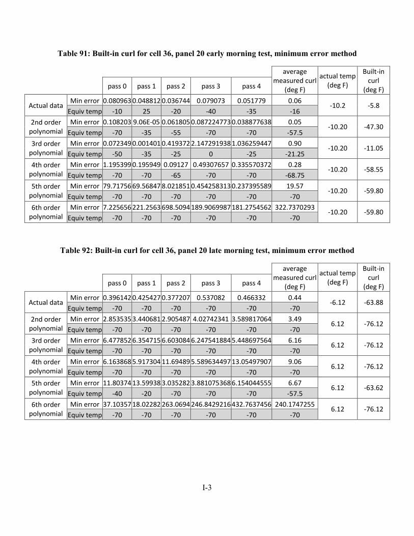
I-3
Table 91: Built-in curl for cell 36, panel 20 early morning test, minimum error method
average
measured curl (deg F)
actual temp (deg F)
Built-in curl
(deg F) pass 0 pass 1 pass 2 pass 3 pass 4
Actual data Min error 0.080963 0.048812 0.036744 0.079073 0.051779 0.06
-10.2 -5.8 Equiv temp -10 25 -20 -40 -35 -16
2nd order polynomial
Min error 0.108203 9.06E-05 0.061805 0.087224773 0.038877638 0.05 -10.20 -47.30
Equiv temp -70 -35 -55 -70 -70 -57.5
3rd order polynomial
Min error 0.072349 0.001401 0.419372 2.147291938 1.036259447 0.90 -10.20 -11.05
Equiv temp -50 -35 -25 0 -25 -21.25
4th order polynomial
Min error 1.195399 0.195949 0.09127 0.49307657 0.335570372 0.28 -10.20 -58.55
Equiv temp -70 -70 -65 -70 -70 -68.75
5th order polynomial
Min error 79.71756 69.56847 8.021851 0.454258313 0.237395589 19.57 -10.20 -59.80
Equiv temp -70 -70 -70 -70 -70 -70
6th order polynomial
Min error 7.225656 221.2563 698.5094 189.9069987 181.2754562 322.7370293 -10.20 -59.80
Equiv temp -70 -70 -70 -70 -70 -70
Table 92: Built-in curl for cell 36, panel 20 late morning test, minimum error method
average
measured curl (deg F)
actual temp (deg F)
Built-in curl
(deg F) pass 0 pass 1 pass 2 pass 3 pass 4
Actual data Min error 0.396142 0.425427 0.377207 0.537082 0.466332 0.44
-6.12 -63.88 Equiv temp -70 -70 -70 -70 -70 -70
2nd order polynomial
Min error 2.853535 3.440681 2.905487 4.02742341 3.589817064 3.49 6.12 -76.12
Equiv temp -70 -70 -70 -70 -70 -70
3rd order polynomial
Min error 6.477852 6.354715 6.603084 6.247541884 5.448697564 6.16 6.12 -76.12
Equiv temp -70 -70 -70 -70 -70 -70
4th order polynomial
Min error 6.163868 5.917304 11.69489 5.589634497 13.05497907 9.06 6.12 -76.12
Equiv temp -70 -70 -70 -70 -70 -70
5th order polynomial
Min error 11.80374 13.59938 3.035282 3.881075368 6.154044555 6.67 6.12 -63.62
Equiv temp -40 -20 -70 -70 -70 -57.5
6th order polynomial
Min error 37.10357 18.02282 263.0694 246.8429216 432.7637456 240.1747255 6.12 -76.12
Equiv temp -70 -70 -70 -70 -70 -70

I-4
Table 93: Built-in curl for cell 37 panel 8 early morning test, minimum error method
average
measured curl (deg F)
actual temp (deg F)
Built-in curl
(deg F) pass 0 pass 1 pass 2 pass 3 pass 4
Actual data Min error 0.088581 0.143342 0.099315 0.176147 0.133989 0.13
-10.43 26.43 Equiv temp -5 30 20 30 5 16
2nd order polynomial
Min error 0.079743 0.386449 0.121896 0.516576911 0.474292243 0.37 -10.43 -59.57
Equiv temp -70 -70 -70 -70 -70 -70
3rd order polynomial
Min error 1.685491 1.519207 0.628588 2.304808767 0.681941493 1.28 -10.43 15.43
Equiv temp 10 20 5 20 -25 5
4th order polynomial
Min error 0.553304 0.657114 0.456182 1.581379047 0.30575202 0.75 -10.43 -44.57
Equiv temp -50 -70 -10 -70 -70 -55
5th order polynomial
Min error 3.338259 6.554003 0.466328 1.696521482 0.34903823 2.27 -10.43 -13.32
Equiv temp 30 30 -10 -50 -65 -23.75
6th order polynomial
Min error 1.510748 5.201621 29.27274 2.404054814 4.398596757 10.31925322 -10.43 -34.57
Equiv temp -25 -70 30 -70 -70 -45
Table 94: Built-in curl for cell 37 panel 8 late morning test, minimum error method
average
measured curl (deg F)
actual temp (deg F)
Built-in curl
(deg F) pass 0 pass 1 pass 2 pass 3 pass 4
Actual data Min error 0.396142 0.425427 0.377207 0.537082 0.466332 0.44
9.75 -79.75 Equiv temp -70 -70 -70 -70 -70 -70
2nd order polynomial
Min error 0.241581 0.825452 0.233871 0.980516582 0.417972377 0.61 9.75 -79.75
Equiv temp -70 -70 -70 -70 -70 -70
3rd order polynomial
Min error 0.127964 1.319183 1.608348 0.274067861 0.753987791 0.99 9.75 -79.75
Equiv temp -70 -70 -70 -70 -70 -70
4th order polynomial
Min error 5.845857 16.00593 3.123215 17.74337002 5.440201145 10.58 9.75 -79.75
Equiv temp -70 -70 -70 -70 -70 -70
5th order polynomial
Min error 85.65234 56.53375 31.91435 59.58761507 42.03130184 47.52 9.75 20.25
Equiv temp 30 30 30 30 30 30
6th order polynomial
Min error 5.931255 66.94493 19.47908 4.883967802 41.45785806 33.19146013 9.75 -29.75
Equiv temp -70 -70 30 -70 30 -20

I-5
Table 95: Built-in curl for cell 37 panel 9 early morning test, minimum error method
average
measured curl (deg F)
actual temp (deg F)
Built-in curl
(deg F) pass 0 pass 1 pass 2 pass 3 pass 4
Actual data Min error 0.088581 0.143342 0.099315 0.176147 0.133989 0.13
-10.43 26.43 Equiv temp -5 30 20 30 5 16
2nd order polynomial
Min error 0.185169 0.257181 0.446429 0.149943117 0.321629677 0.29 -10.43 -59.57
Equiv temp -50 -70 -70 -70 -70 -70
3rd order polynomial
Min error 0.432182 0.794688 1.555451 1.378773174 1.504621428 1.31 -10.43 24.18
Equiv temp 20 20 15 10 10 13.75
4th order polynomial
Min error 0.3958 0.358906 0.515918 0.382463306 0.457532288 0.43 -10.43 -47.07
Equiv temp -65 -20 -70 -70 -70 -57.5
5th order polynomial
Min error 14.14257 12.64561 26.56274 0.421432754 2.018907963 10.41 -10.43 6.68
Equiv temp 30 30 30 -65 -10 -3.75
6th order polynomial
Min error 2.513289 17.4773 5.611443 23.50603871 0.999160037 11.89848465 -10.43 -59.57
Equiv temp 30 -70 -70 -70 -70 -70
Table 96: Built-in curl for cell 37 panel 9 late morning test, minimum error method
average
measured curl (deg F)
actual temp (deg F)
Built-in curl
(deg F) pass 0 pass 1 pass 2 pass 3 pass 4
Actual data Min error 0.34442 0.241389 0.26168 0.204257 0.196421 0.25
9.75 -70.75 Equiv temp -50 -70 -65 -50 -70 -61
2nd order polynomial
Min error 0.403364 0.117308 0.86721 0.60647857 0.481333447 0.52 9.75 -79.75
Equiv temp -70 -70 -70 -70 -70 -70
3rd order polynomial
Min error 2.08267 0.853075 1.040265 0.53324492 0.50583126 0.73 9.75 -79.75
Equiv temp -70 -70 -70 -70 -70 -70
4th order polynomial
Min error 16.41969 0.925517 13.90184 8.640068553 9.306155304 8.19 9.75 -79.75
Equiv temp -70 -70 -70 -70 -70 -70
5th order polynomial
Min error 82.98905 98.63693 46.57671 43.53981886 53.6212543 60.59 9.75 20.25
Equiv temp 30 30 30 30 30 30
6th order polynomial
Min error 57.66396 2.457863 218.0958 21.00232926 6.716629483 62.06814659 9.75 -79.75
Equiv temp -70 -70 -70 -70 -70 -70
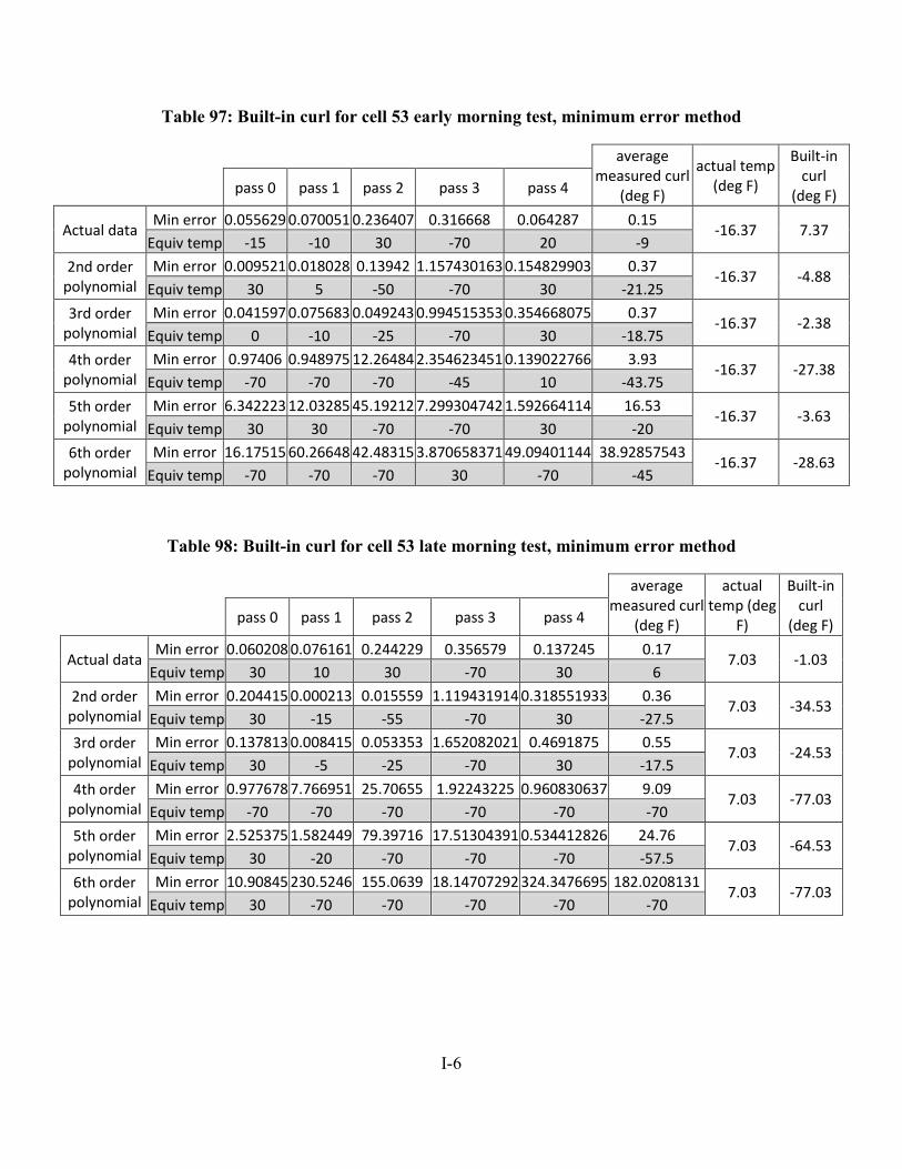
I-6
Table 97: Built-in curl for cell 53 early morning test, minimum error method
average
measured curl (deg F)
actual temp (deg F)
Built-in curl
(deg F) pass 0 pass 1 pass 2 pass 3 pass 4
Actual data Min error 0.055629 0.070051 0.236407 0.316668 0.064287 0.15
-16.37 7.37 Equiv temp -15 -10 30 -70 20 -9
2nd order polynomial
Min error 0.009521 0.018028 0.13942 1.157430163 0.154829903 0.37 -16.37 -4.88
Equiv temp 30 5 -50 -70 30 -21.25
3rd order polynomial
Min error 0.041597 0.075683 0.049243 0.994515353 0.354668075 0.37 -16.37 -2.38
Equiv temp 0 -10 -25 -70 30 -18.75
4th order polynomial
Min error 0.97406 0.948975 12.26484 2.354623451 0.139022766 3.93 -16.37 -27.38
Equiv temp -70 -70 -70 -45 10 -43.75
5th order polynomial
Min error 6.342223 12.03285 45.19212 7.299304742 1.592664114 16.53 -16.37 -3.63
Equiv temp 30 30 -70 -70 30 -20
6th order polynomial
Min error 16.17515 60.26648 42.48315 3.870658371 49.09401144 38.92857543 -16.37 -28.63
Equiv temp -70 -70 -70 30 -70 -45
Table 98: Built-in curl for cell 53 late morning test, minimum error method
average
measured curl (deg F)
actual temp (deg
F)
Built-in curl
(deg F) pass 0 pass 1 pass 2 pass 3 pass 4
Actual data Min error 0.060208 0.076161 0.244229 0.356579 0.137245 0.17
7.03 -1.03 Equiv temp 30 10 30 -70 30 6
2nd order polynomial
Min error 0.204415 0.000213 0.015559 1.119431914 0.318551933 0.36 7.03 -34.53
Equiv temp 30 -15 -55 -70 30 -27.5
3rd order polynomial
Min error 0.137813 0.008415 0.053353 1.652082021 0.4691875 0.55 7.03 -24.53
Equiv temp 30 -5 -25 -70 30 -17.5
4th order polynomial
Min error 0.977678 7.766951 25.70655 1.92243225 0.960830637 9.09 7.03 -77.03
Equiv temp -70 -70 -70 -70 -70 -70
5th order polynomial
Min error 2.525375 1.582449 79.39716 17.51304391 0.534412826 24.76 7.03 -64.53
Equiv temp 30 -20 -70 -70 -70 -57.5
6th order polynomial
Min error 10.90845 230.5246 155.0639 18.14707292 324.3476695 182.0208131 7.03 -77.03
Equiv temp 30 -70 -70 -70 -70 -70

I-7
Table 99: Built-in curl for cell 71, minimum error method
average
measured curl (deg F)
actual temp (deg F)
Built-in curl
(deg F) pass 0 pass 1 pass 2 pass 3 pass 4
Actual data Min error 0.091632 0.070345 0.105909 0.09583 0.083409 0.09
-10.29 -43.71 Equiv temp -65 -60 -30 -65 -50 -54
2nd order polynomial
Min error 0.255274 0.171656 0.181797 0.172753314 0.114843414 0.16 -10.29 -59.71
Equiv temp -70 -70 -70 -70 -70 -70
3rd order polynomial
Min error 0.334994 0.361935 0.458965 0.704934007 0.568124154 0.52 -10.29 -54.71
Equiv temp -70 -70 -65 -65 -60 -65
4th order polynomial
Min error 0.345739 0.394229 0.593048 0.704656639 0.556399336 0.56 -10.29 -59.71
Equiv temp -70 -70 -70 -70 -70 -70
5th order polynomial
Min error 0.787658 1.285469 1.097877 1.271543977 1.745440313 1.35 -10.29 -59.71
Equiv temp -70 -70 -70 -70 -70 -70
6th order polynomial
Min error 2.201241 0.983339 1.820265 1.552549426 1.833406995 1.547389875 -10.29 40.29
Equiv temp 30 30 30 30 30 30
Table 100: Built-in curl for cell 72, minimum error method
average
measured curl (deg F)
actual temp (deg F)
Built-in curl
(deg F) pass 0 pass 1 pass 2 pass 3 pass 4
Actual data Min error 0.086517 0.057372 0.026249 0.035211 0.100173 0.06
-9.99 -59.01 Equiv temp -70 -65 -70 -70 -70 -69
2nd order polynomial
Min error 0.566675 0.414486 0.590912 0.236859049 0.456956052 0.42 -9.99 -60.01
Equiv temp -70 -70 -70 -70 -70 -70
3rd order polynomial
Min error 0.336034 0.243411 0.810923 0.162545115 0.489255117 0.43 -9.99 -60.01
Equiv temp -70 -70 -70 -70 -70 -70
4th order polynomial
Min error 0.200611 0.27915 1.911832 0.145682754 0.470123784 0.70 -9.99 -60.01
Equiv temp -70 -70 -70 -70 -70 -70
5th order polynomial
Min error 0.215068 0.360756 6.650767 0.661595725 4.873669941 3.14 -9.99 -60.01
Equiv temp -70 -70 -70 -70 -70 -70
6th order polynomial
Min error 0.288598 5.685872 6.782297 0.864367609 17.2557728 7.647077271 -9.99 -32.51
Equiv temp -70 30 -70 -60 -70 -42.5
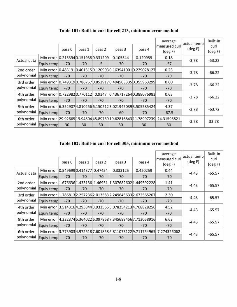
I-8
Table 101: Built-in curl for cell 213, minimum error method
average
measured curl (deg F)
actual temp (deg F)
Built-in curl
(deg F) pass 0 pass 1 pass 2 pass 3 pass 4
Actual data Min error 0.215394 0.151938 0.331209 0.105344 0.120959 0.18
-3.78 -53.22 Equiv temp -70 -70 -5 -70 -70 -57
2nd order polynomial
Min error 0.483191 0.401315 0.120903 0.163941001 0.229028127 0.23 -3.78 -66.22
Equiv temp -70 -70 -70 -70 -70 -70
3rd order polynomial
Min error 0.749319 0.786757 0.852917 0.404503335 0.355963299 0.60 -3.78 -66.22
Equiv temp -70 -70 -70 -70 -70 -70
4th order polynomial
Min error 0.722982 0.770112 0.9347 0.436717264 0.388076983 0.63 -3.78 -66.22
Equiv temp -70 -70 -70 -70 -70 -70
5th order polynomial
Min error 6.352907 4.810256 6.150212 3.021945039 3.505585424 4.37 -3.78 -63.72
Equiv temp -70 -70 -70 -60 -70 -67.5
6th order polynomial
Min error 29.92665 19.94804 45.89769 19.62816843 11.78997239 24.31596821 -3.78 33.78
Equiv temp 30 30 30 30 30 30
Table 102: Built-in curl for cell 305, minimum error method
average
measured curl (deg F)
actual temp (deg F)
Built-in curl
(deg F) pass 0 pass 1 pass 2 pass 3 pass 4
Actual data Min error 0.549699 0.414377 0.47454 0.333125 0.420259 0.44
-4.43 -65.57 Equiv temp -70 -70 -70 -70 -70 -70
2nd order polynomial
Min error 1.676636 1.433136 1.46951 1.307682602 1.449592228 1.41 -4.43 -65.57
Equiv temp -70 -70 -70 -70 -70 -70
3rd order polynomial
Min error 1.786813 2.257236 2.013583 2.249645633 2.672565207 2.30 -4.43 -65.57
Equiv temp -70 -70 -70 -70 -70 -70
4th order polynomial
Min error 3.514316 4.295844 3.933565 5.078254213 4.768828256 4.52 -4.43 -65.57
Equiv temp -70 -70 -70 -70 -70 -70
5th order polynomial
Min error 4.222374 5.364022 6.097868 7.345688456 7.713058916 6.63 -4.43 -65.57
Equiv temp -70 -70 -70 -70 -70 -70
6th order polynomial
Min error 3.773903 4.972618 7.601858 6.811073122 9.711754965 7.274326062 -4.43 -65.57
Equiv temp -70 -70 -70 -70 -70 -70

I-9
Table 103: Built-in curl for cell 513, minimum error method
average
measured curl (deg F)
actual temp (deg F)
Built-in curl
(deg F) pass 0 pass 1 pass 2 pass 3 pass 4
Actual data Min error 0.119136 0.182213 0.14834 0.192701 0.262575 0.18
-3.78 -64.22 Equiv temp -70 -60 -70 -70 -70 -68
2nd order polynomial
Min error 0.47436 0.768367 0.676498 0.884753559 1.091192913 0.86 -3.78 -61.22
Equiv temp -70 -55 -70 -70 -65 -65
3rd order polynomial
Min error 0.791149 3.382765 2.129828 2.994757844 2.4539242 2.74 -3.78 -63.72
Equiv temp -70 -60 -70 -70 -70 -67.5
4th order polynomial
Min error 22.63493 11.44746 16.94271 26.96238499 30.36808992 21.43 -3.78 -66.22
Equiv temp -70 -70 -70 -70 -70 -70
5th order polynomial
Min error 3.515314 10.87874 15.43252 10.21479288 18.09782613 13.66 -3.78 -66.22
Equiv temp -70 -70 -70 -70 -70 -70
6th order polynomial
Min error 13.7047 162.3762 135.8292 58.56661503 67.16433766 105.9840914 -3.78 -16.22
Equiv temp 30 -70 30 30 -70 -20
Table 104: Built-in curl for cell 614, minimum error method
average
measured curl (deg F)
actual temp (deg F)
Built-in curl
(deg F) pass 0 pass 1 pass 2 pass 3 pass 4
Actual data Min error 0.346344 0.189199 0.188507 0.292815 0.201453 0.24
-3.78 -61.22 Equiv temp -65 -65 -65 -65 -65 -65
2nd order polynomial
Min error 1.439683 0.864841 0.763571 1.532184734 3.298453979 1.61 -3.78 -37.47
Equiv temp -65 -65 -65 -65 30 -41.25
3rd order polynomial
Min error 0.712723 0.909993 0.884926 1.541845562 18.91753227 5.56 -3.78 -37.47
Equiv temp -65 -65 -65 -65 30 -41.25
4th order polynomial
Min error 0.932584 2.346939 2.986821 2.913922095 80.10558841 22.09 -3.78 -37.47
Equiv temp -65 -65 -65 -65 30 -41.25
5th order polynomial
Min error 2.391748 6.775033 7.078198 12.77618792 234.8453254 65.37 -3.78 -37.47
Equiv temp -65 -65 -65 -65 30 -41.25
6th order polynomial
Min error 42.31462 25.60408 23.50462 65.42864388 1719.115346 458.4131724 -3.78 31.28
Equiv temp 30 30 20 30 30 27.5

APPENDIX J: BUILT-IN CURL AS DETERMINED FROM MINIMUM ERROR METHOD FOR HALF SLABS
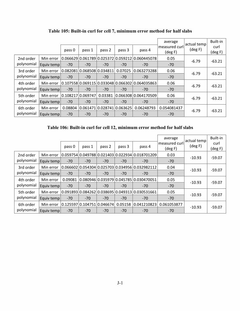
J-1
Table 105: Built-in curl for cell 7, minimum error method for half slabs
average
measured curl (deg F)
actual temp (deg F)
Built-in curl
(deg F) pass 0 pass 1 pass 2 pass 3 pass 4
2nd order polynomial
Min error 0.066629 0.061789 0.025372 0.059212 0.060445078 0.05 -6.79 -63.21
Equiv temp -70 -70 -70 -70 -70 -70
3rd order polynomial
Min error 0.082081 0.068508 0.034811 0.07025 0.063273288 0.06 -6.79 -63.21
Equiv temp -70 -70 -70 -70 -70 -70
4th order polynomial
Min error 0.107558 0.069115 0.033048 0.066302 0.064035863 0.06 -6.79 -63.21
Equiv temp -70 -70 -70 -70 -70 -70
5th order polynomial
Min error 0.108217 0.069747 0.03381 0.066308 0.064170509 0.06 -6.79 -63.21
Equiv temp -70 -70 -70 -70 -70 -70
6th order polynomial
Min error 0.08804 0.061471 0.028741 0.063625 0.06248793 0.054081437 -6.79 -63.21
Equiv temp -70 -70 -70 -70 -70 -70
Table 106: Built-in curl for cell 12, minimum error method for half slabs
average
measured curl (deg F)
actual temp (deg F)
Built-in curl
(deg F) pass 0 pass 1 pass 2 pass 3 pass 4
2nd order polynomial
Min error 0.059754 0.049788 0.021403 0.022934 0.018701209 0.03 -10.93 -59.07
Equiv temp -70 -70 -70 -70 -70 -70
3rd order polynomial
Min error 0.066602 0.054304 0.025703 0.034956 0.032982112 0.04 -10.93 -59.07
Equiv temp -70 -70 -70 -70 -70 -70
4th order polynomial
Min error 0.09081 0.080946 0.035979 0.045785 0.030470051 0.05 -10.93 -59.07
Equiv temp -70 -70 -70 -70 -70 -70
5th order polynomial
Min error 0.091893 0.084262 0.038695 0.049313 0.030531661 0.05 -10.93 -59.07
Equiv temp -70 -70 -70 -70 -70 -70
6th order polynomial
Min error 0.125597 0.104751 0.046674 0.05158 0.041210823 0.061053877 -10.93 -59.07
Equiv temp -70 -70 -70 -70 -70 -70
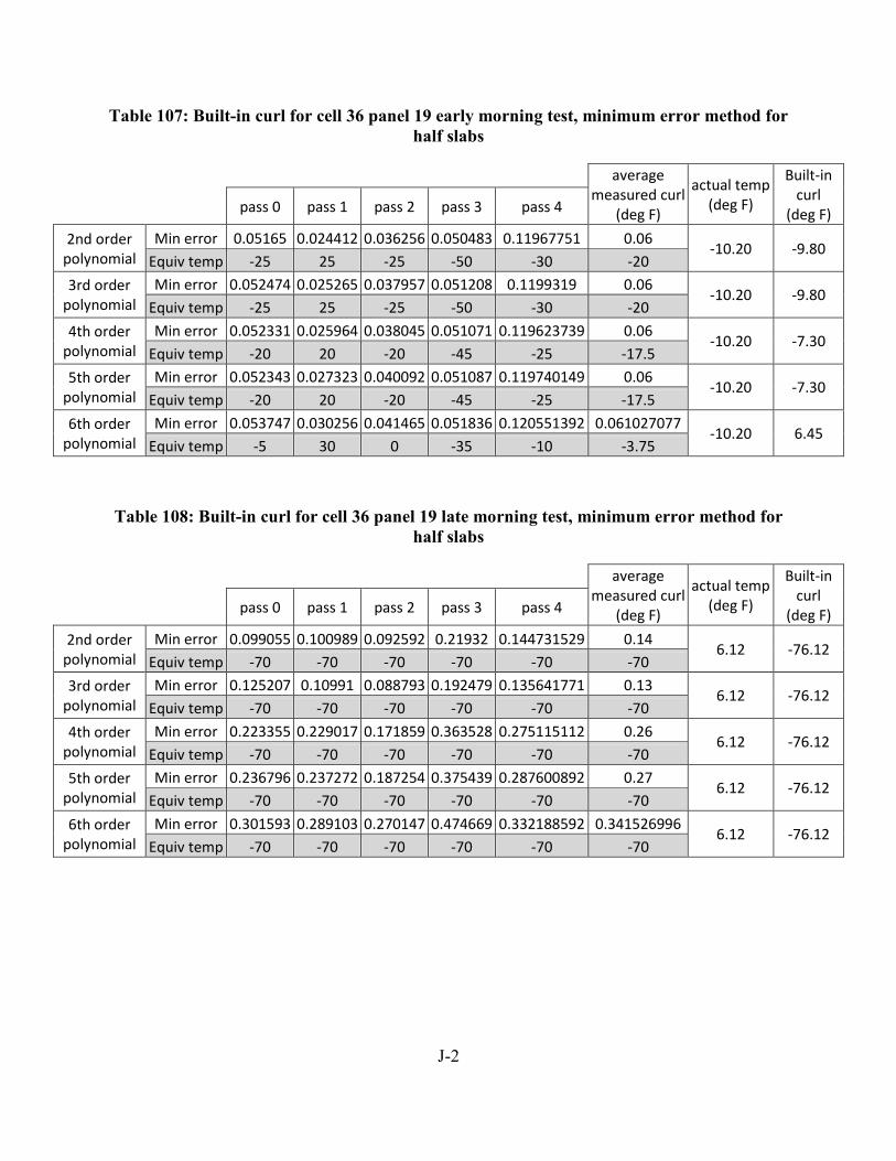
J-2
Table 107: Built-in curl for cell 36 panel 19 early morning test, minimum error method for half slabs
average
measured curl (deg F)
actual temp (deg F)
Built-in curl
(deg F) pass 0 pass 1 pass 2 pass 3 pass 4
2nd order polynomial
Min error 0.05165 0.024412 0.036256 0.050483 0.11967751 0.06 -10.20 -9.80
Equiv temp -25 25 -25 -50 -30 -20
3rd order polynomial
Min error 0.052474 0.025265 0.037957 0.051208 0.1199319 0.06 -10.20 -9.80
Equiv temp -25 25 -25 -50 -30 -20
4th order polynomial
Min error 0.052331 0.025964 0.038045 0.051071 0.119623739 0.06 -10.20 -7.30
Equiv temp -20 20 -20 -45 -25 -17.5
5th order polynomial
Min error 0.052343 0.027323 0.040092 0.051087 0.119740149 0.06 -10.20 -7.30
Equiv temp -20 20 -20 -45 -25 -17.5
6th order polynomial
Min error 0.053747 0.030256 0.041465 0.051836 0.120551392 0.061027077 -10.20 6.45
Equiv temp -5 30 0 -35 -10 -3.75
Table 108: Built-in curl for cell 36 panel 19 late morning test, minimum error method for half slabs
average
measured curl (deg F)
actual temp (deg F)
Built-in curl
(deg F) pass 0 pass 1 pass 2 pass 3 pass 4
2nd order polynomial
Min error 0.099055 0.100989 0.092592 0.21932 0.144731529 0.14 6.12 -76.12
Equiv temp -70 -70 -70 -70 -70 -70
3rd order polynomial
Min error 0.125207 0.10991 0.088793 0.192479 0.135641771 0.13 6.12 -76.12
Equiv temp -70 -70 -70 -70 -70 -70
4th order polynomial
Min error 0.223355 0.229017 0.171859 0.363528 0.275115112 0.26 6.12 -76.12
Equiv temp -70 -70 -70 -70 -70 -70
5th order polynomial
Min error 0.236796 0.237272 0.187254 0.375439 0.287600892 0.27 6.12 -76.12
Equiv temp -70 -70 -70 -70 -70 -70
6th order polynomial
Min error 0.301593 0.289103 0.270147 0.474669 0.332188592 0.341526996 6.12 -76.12
Equiv temp -70 -70 -70 -70 -70 -70

J-3
Table 109: Built-in curl for cell 36 panel 20 early morning test, minimum error method for half slabs
average
measured curl (deg F)
actual temp (deg F)
Built-in curl
(deg F) pass 0 pass 1 pass 2 pass 3 pass 4
2nd order polynomial
Min error 0.009597 0.000706 0.006914 0.008303 0.005461707 0.01 -10.20 -27.30
Equiv temp -45 -35 -50 -35 -30 -37.5
3rd order polynomial
Min error 0.0096 0.00138 0.006936 0.008483 0.006138567 0.01 -10.20 -27.30
Equiv temp -45 -35 -50 -35 -30 -37.5
4th order polynomial
Min error 0.010345 0.00304 0.011488 0.008987 0.006145488 0.01 -10.20 -17.30
Equiv temp -35 -20 -30 -30 -30 -27.5
5th order polynomial
Min error 0.012237 0.003817 0.011812 0.009399 0.006149906 0.01 -10.20 -17.30
Equiv temp -35 -20 -30 -30 -30 -27.5
6th order polynomial
Min error 0.01504 0.006716 0.012788 0.010579 0.006588244 0.009167782 -10.20 -9.80
Equiv temp -20 -5 -25 -25 -25 -20
Table 110: Built-in curl for cell 36 panel 20 late morning test, minimum error method for half slabs
average
measured curl (deg F)
actual temp (deg F)
Built-in curl
(deg F) pass 0 pass 1 pass 2 pass 3 pass 4
2nd order polynomial
Min error 0.663431 0.841624 0.802039 0.941298 0.835531187 0.86 6.12 -76.12
Equiv temp -70 -70 -70 -70 -70 -70
3rd order polynomial
Min error 0.684292 0.87594 0.833154 0.957996 0.858616592 0.88 6.12 -76.12
Equiv temp -70 -70 -70 -70 -70 -70
4th order polynomial
Min error 0.760486 0.94038 0.867154 1.067027 0.993096131 0.97 6.12 -76.12
Equiv temp -70 -70 -70 -70 -70 -70
5th order polynomial
Min error 0.765446 0.953351 0.882754 1.078398 1.003951756 0.98 6.12 -76.12
Equiv temp -70 -70 -70 -70 -70 -70
6th order polynomial
Min error 0.798874 1.021963 0.957032 1.183406 1.096450657 1.064713064 6.12 -76.12
Equiv temp -70 -70 -70 -70 -70 -70

J-4
Table 111: Built-in curl for cell 37 panel 8 early morning test, minimum error method for half slabs
average
measured curl (deg F)
actual temp (deg F)
Built-in curl
(deg F) pass 0 pass 1 pass 2 pass 3 pass 4
2nd order polynomial
Min error 0.022666 0.082517 0.044507 0.083538 0.073631743 0.07 -10.43 22.93
Equiv temp -5 20 10 30 -10 12.5
3rd order polynomial
Min error 0.024783 0.083099 0.044955 0.083727 0.075219108 0.07 -10.43 22.93
Equiv temp -5 20 10 30 -10 12.5
4th order polynomial
Min error 0.026571 0.083129 0.045621 0.093419 0.075133705 0.07 -10.43 31.68
Equiv temp 15 30 25 30 0 21.25
5th order polynomial
Min error 0.026733 0.083801 0.046445 0.096251 0.075435173 0.08 -10.43 31.68
Equiv temp 15 30 25 30 0 21.25
6th order polynomial
Min error 0.030777 0.089732 0.051114 0.105442 0.077193604 0.080870293 -10.43 37.93
Equiv temp 30 30 30 30 20 27.5
Table 112: Built-in curl for cell 37 panel 8 late morning test, minimum error method for half slabs
average
measured curl (deg F)
actual temp (deg F)
Built-in curl
(deg F) pass 0 pass 1 pass 2 pass 3 pass 4
2nd order polynomial
Min error 0.042142 0.078469 0.05907 0.044038 0.057822831 0.06 9.75 -79.75
Equiv temp -70 -70 -70 -70 -70 -70
3rd order polynomial
Min error 0.048551 0.088147 0.070694 0.062114 0.072693223 0.07 9.75 -79.75
Equiv temp -70 -70 -70 -70 -70 -70
4th order polynomial
Min error 0.146049 0.192533 0.182539 0.126719 0.148450909 0.16 9.75 -79.75
Equiv temp -70 -70 -70 -70 -70 -70
5th order polynomial
Min error 0.146049 0.192614 0.182872 0.130121 0.149884855 0.16 9.75 -79.75
Equiv temp -70 -70 -70 -70 -70 -70
6th order polynomial
Min error 0.197224 0.247958 0.245226 0.176664 0.207068199 0.219228921 9.75 -79.75
Equiv temp -70 -70 -70 -70 -70 -70

J-5
Table 113: Built-in curl for cell 37 panel 9 early morning test, minimum error method for half slabs
average
measured curl (deg F)
actual temp (deg F)
Built-in curl
(deg F) pass 0 pass 1 pass 2 pass 3 pass 4
2nd order polynomial
Min error 0.038575 0.067846 0.078154 0.037475 0.060518277 0.06 -10.43 12.93
Equiv temp 0 0 -25 30 5 2.5
3rd order polynomial
Min error 0.038604 0.072499 0.080455 0.039283 0.062324102 0.06 -10.43 12.93
Equiv temp 0 0 -25 30 5 2.5
4th order polynomial
Min error 0.039359 0.072968 0.080556 0.043328 0.064323299 0.07 -10.43 15.43
Equiv temp -10 -5 -30 30 25 5
5th order polynomial
Min error 0.042497 0.073286 0.080587 0.043913 0.064736276 0.07 -10.43 15.43
Equiv temp -10 -5 -30 30 25 5
6th order polynomial
Min error 0.04642 0.075875 0.081222 0.058532 0.072311888 0.071985121 -10.43 27.93
Equiv temp 25 20 -10 30 30 17.5
Table 114: Built-in curl for cell 37 panel 9 late morning test, minimum error method for half slabs
average
measured curl (deg F)
actual temp (deg F)
Built-in curl
(deg F) pass 0 pass 1 pass 2 pass 3 pass 4
2nd order polynomial
Min error 0.075388 0.082941 0.077863 0.059823 0.059359452 0.07 9.75 -79.75
Equiv temp -70 -70 -70 -70 -70 -70
3rd order polynomial
Min error 0.088252 0.085726 0.079697 0.065836 0.066407707 0.07 9.75 -79.75
Equiv temp -70 -70 -70 -70 -70 -70
4th order polynomial
Min error 0.255112 0.249236 0.173015 0.145994 0.160556867 0.18 9.75 -79.75
Equiv temp -70 -70 -70 -70 -70 -70
5th order polynomial
Min error 0.255305 0.249432 0.173258 0.146204 0.160635441 0.18 9.75 -79.75
Equiv temp -70 -70 -70 -70 -70 -70
6th order polynomial
Min error 0.283902 0.291647 0.185415 0.166475 0.191728161 0.208816207 9.75 -79.75
Equiv temp -70 -70 -70 -70 -70 -70

J-6
Table 115: Built-in curl for cell 53 early morning test, minimum error method for half slabs
average
measured curl (deg F)
actual temp (deg F)
Built-in curl
(deg F) pass 0 pass 1 pass 2 pass 3 pass 4
2nd order polynomial
Min error 0.009975 2.19E-05 0.024857 0.002786 0.018370594 0.01 -16.37 2.62
Equiv temp -30 -45 30 -70 30 -13.75
3rd order polynomial
Min error 0.010954 2.48E-05 0.030554 0.005228 0.018584083 0.01 -16.37 2.62
Equiv temp -30 -45 30 -70 30 -13.75
4th order polynomial
Min error 0.023954 0.012304 0.123062 0.004783 0.019694343 0.04 -16.37 -3.63
Equiv temp -70 -70 30 -70 30 -20
5th order polynomial
Min error 0.024826 0.012336 0.125453 0.008984 0.019694655 0.04 -16.37 -3.63
Equiv temp -70 -70 30 -70 30 -20
6th order polynomial
Min error 0.022964 0.013429 0.173959 0.011702 0.01908959 0.054544879 -16.37 -3.63
Equiv temp -65 -70 30 -70 30 -20
Table 116: Built-in curl for cell 53 late morning test, minimum error method for half slabs
average
measured curl (deg F)
actual temp (deg F)
Built-in curl
(deg F) pass 0 pass 1 pass 2 pass 3 pass 4
2nd order polynomial
Min error 0.022291 0.007451 0.033451 0.035859 0.061550311 0.03 7.03 4.22
Equiv temp 30 25 30 -40 30 11.25
3rd order polynomial
Min error 0.026234 0.007608 0.043371 0.035866 0.061903079 0.04 7.03 4.22
Equiv temp 30 25 30 -40 30 11.25
4th order polynomial
Min error 0.028046 0.009798 0.15518 0.037105 0.068324059 0.07 7.03 0.47
Equiv temp 30 -5 30 -25 30 7.5
5th order polynomial
Min error 0.028166 0.010441 0.157794 0.038957 0.069106202 0.07 7.03 0.47
Equiv temp 30 -5 30 -25 30 7.5
6th order polynomial
Min error 0.027917 0.010513 0.20395 0.038594 0.066743754 0.079950509 7.03 -2.03
Equiv temp 30 -5 30 -35 30 5
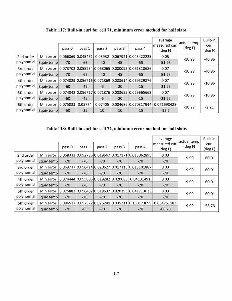
J-7
Table 117: Built-in curl for cell 71, minimum error method for half slabs
average
measured curl (deg F)
actual temp (deg F)
Built-in curl
(deg F) pass 0 pass 1 pass 2 pass 3 pass 4
2nd order polynomial
Min error 0.066869 0.045461 0.05932 0.067921 0.045422225 0.05 -10.29 -40.96
Equiv temp -70 -65 -40 -45 -55 -51.25
3rd order polynomial
Min error 0.073702 0.055254 0.068065 0.080095 0.061310686 0.07 -10.29 -40.96
Equiv temp -70 -65 -40 -45 -55 -51.25
4th order polynomial
Min error 0.074029 0.056716 0.071869 0.083614 0.069529876 0.07 -10.29 -10.96
Equiv temp -60 -45 -5 -20 -15 -21.25
5th order polynomial
Min error 0.074042 0.056717 0.071876 0.083652 0.069665663 0.07 -10.29 -10.96
Equiv temp -60 -45 -5 -20 -15 -21.25
6th order polynomial
Min error 0.075033 0.05774 0.07405 0.084686 0.070317944 0.071698428 -10.29 -2.21
Equiv temp -50 -35 10 -10 -15 -12.5
Table 118: Built-in curl for cell 72, minimum error method for half slabs
average
measured curl (deg F)
actual temp (deg F)
Built-in curl
(deg F) pass 0 pass 1 pass 2 pass 3 pass 4
2nd order polynomial
Min error 0.068333 0.052736 0.019667 0.017171 0.015062895 0.03 -9.99 -60.01
Equiv temp -70 -70 -70 -70 -70 -70
3rd order polynomial
Min error 0.069737 0.056414 0.020627 0.017315 0.015101887 0.03 -9.99 -60.01
Equiv temp -70 -70 -70 -70 -70 -70
4th order polynomial
Min error 0.074444 0.055806 0.019282 0.020083 0.04131491 0.03 -9.99 -60.01
Equiv temp -70 -70 -70 -70 -70 -70
5th order polynomial
Min error 0.075882 0.056482 0.019637 0.020395 0.041713623 0.03 -9.99 -60.01
Equiv temp -70 -70 -70 -70 -70 -70
6th order polynomial
Min error 0.086517 0.057372 0.026249 0.035211 0.100173099 0.054751183 -9.99 -58.76
Equiv temp -70 -65 -70 -70 -70 -68.75
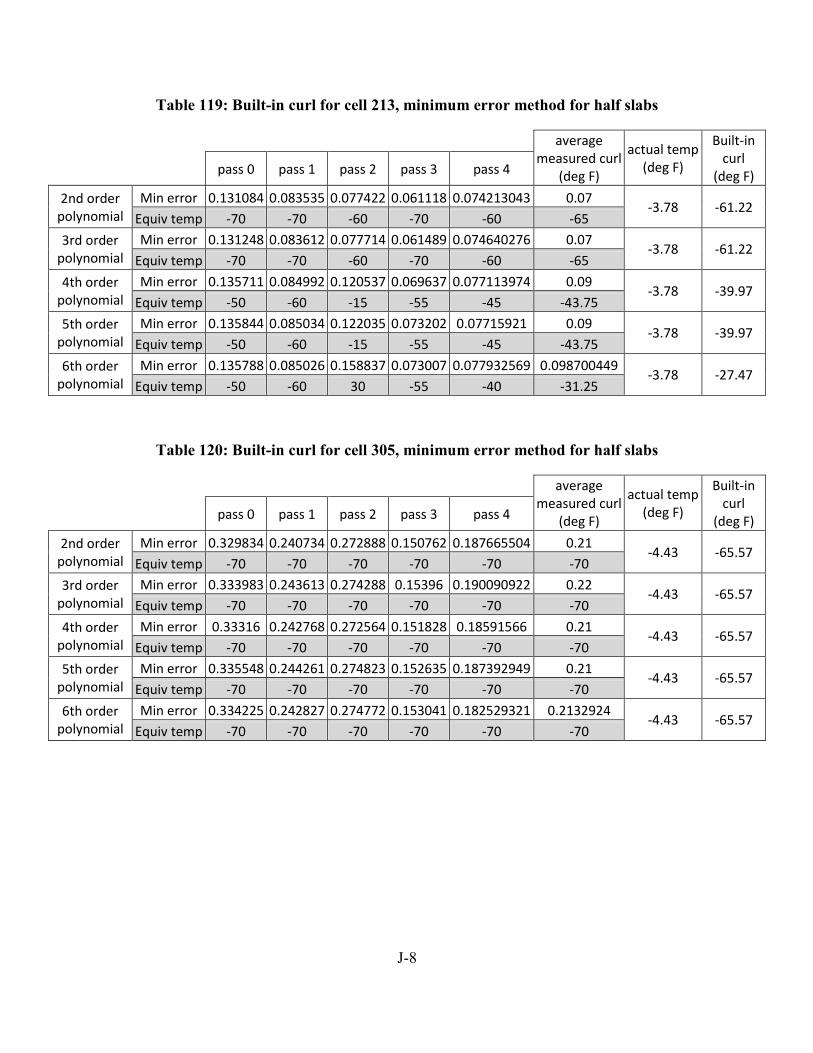
J-8
Table 119: Built-in curl for cell 213, minimum error method for half slabs
average
measured curl (deg F)
actual temp (deg F)
Built-in curl
(deg F) pass 0 pass 1 pass 2 pass 3 pass 4
2nd order polynomial
Min error 0.131084 0.083535 0.077422 0.061118 0.074213043 0.07 -3.78 -61.22
Equiv temp -70 -70 -60 -70 -60 -65
3rd order polynomial
Min error 0.131248 0.083612 0.077714 0.061489 0.074640276 0.07 -3.78 -61.22
Equiv temp -70 -70 -60 -70 -60 -65
4th order polynomial
Min error 0.135711 0.084992 0.120537 0.069637 0.077113974 0.09 -3.78 -39.97
Equiv temp -50 -60 -15 -55 -45 -43.75
5th order polynomial
Min error 0.135844 0.085034 0.122035 0.073202 0.07715921 0.09 -3.78 -39.97
Equiv temp -50 -60 -15 -55 -45 -43.75
6th order polynomial
Min error 0.135788 0.085026 0.158837 0.073007 0.077932569 0.098700449 -3.78 -27.47
Equiv temp -50 -60 30 -55 -40 -31.25
Table 120: Built-in curl for cell 305, minimum error method for half slabs
average
measured curl (deg F)
actual temp (deg F)
Built-in curl
(deg F) pass 0 pass 1 pass 2 pass 3 pass 4
2nd order polynomial
Min error 0.329834 0.240734 0.272888 0.150762 0.187665504 0.21 -4.43 -65.57
Equiv temp -70 -70 -70 -70 -70 -70
3rd order polynomial
Min error 0.333983 0.243613 0.274288 0.15396 0.190090922 0.22 -4.43 -65.57
Equiv temp -70 -70 -70 -70 -70 -70
4th order polynomial
Min error 0.33316 0.242768 0.272564 0.151828 0.18591566 0.21 -4.43 -65.57
Equiv temp -70 -70 -70 -70 -70 -70
5th order polynomial
Min error 0.335548 0.244261 0.274823 0.152635 0.187392949 0.21 -4.43 -65.57
Equiv temp -70 -70 -70 -70 -70 -70
6th order polynomial
Min error 0.334225 0.242827 0.274772 0.153041 0.182529321 0.2132924 -4.43 -65.57
Equiv temp -70 -70 -70 -70 -70 -70

J-9
Table 121: Built-in curl for cell 513, minimum error method for half slabs
average
measured curl (deg F)
actual temp (deg F)
Built-in curl
(deg F) pass 0 pass 1 pass 2 pass 3 pass 4
2nd order polynomial
Min error 0.061027 0.104558 0.089252 0.120152 0.14856124 0.1156 -3.78 -53.72
Equiv temp -70 -45 -70 -60 -55 -57.5
3rd order polynomial
Min error 0.061155 0.107205 0.090441 0.121961 0.14938364 0.1172 -3.78 -53.72
Equiv temp -70 -45 -70 -60 -55 -57.5
4th order polynomial
Min error 0.06674 0.108476 0.093352 0.127257 0.156006649 0.1213 -3.78 -32.47
Equiv temp -50 -30 -50 -40 -25 -36.25
5th order polynomial
Min error 0.066766 0.108848 0.093423 0.127262 0.15602721 0.1214 -3.78 -32.47
Equiv temp -50 -30 -50 -40 -25 -36.25
6th order polynomial
Min error 0.067621 0.108931 0.094795 0.128592 0.155833681 0.122038002 -3.78 -32.47
Equiv temp -50 -35 -45 -35 -30 -36.25
Table 122: Built-in curl for cell 614, minimum error method for half slabs
average
measured curl (deg F)
actual temp (deg F)
Built-in curl
(deg F) pass 0 pass 1 pass 2 pass 3 pass 4
2nd order polynomial
Min error 0.172106 0.113442 0.083798 0.142812 0.146642537 0.12 -3.78 -32.47
Equiv temp -70 -60 -50 -65 30 -36.25
3rd order polynomial
Min error 0.172402 0.113458 0.083798 0.143835 0.159303769 0.13 -3.78 -32.47
Equiv temp -70 -60 -50 -65 30 -36.25
4th order polynomial
Min error 0.172215 0.11509 0.085837 0.143 0.161251915 0.13 -3.78 -23.72
Equiv temp -55 -40 -20 -65 15 -27.5
5th order polynomial
Min error 0.172238 0.115259 0.086297 0.143004 0.166911285 0.13 -3.78 -23.72
Equiv temp -55 -40 -20 -65 15 -27.5
6th order polynomial
Min error 0.174347 0.115249 0.08683 0.143422 0.171322107 0.129206057 -3.78 -16.22
Equiv temp -70 -40 -5 -65 30 -20

APPENDIX K: POLYNOMIAL CURVATURE METHOD STATISTICS
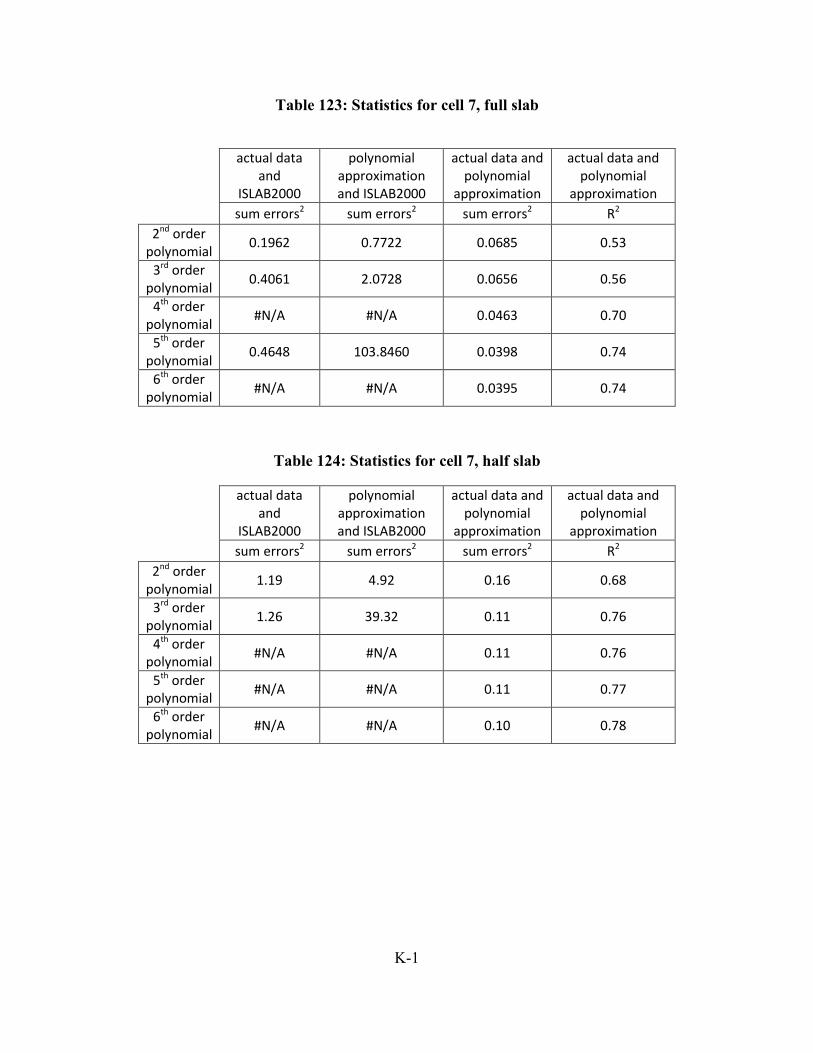
K-1
Table 123: Statistics for cell 7, full slab
actual data and
ISLAB2000
polynomial approximation and ISLAB2000
actual data and polynomial
approximation
actual data and polynomial
approximation
sum errors2 sum errors2 sum errors2 R2
2nd order polynomial
0.1962 0.7722 0.0685 0.53
3rd order polynomial
0.4061 2.0728 0.0656 0.56
4th order polynomial
#N/A #N/A 0.0463 0.70
5th order polynomial
0.4648 103.8460 0.0398 0.74
6th order polynomial
#N/A #N/A 0.0395 0.74
Table 124: Statistics for cell 7, half slab
actual data and
ISLAB2000
polynomial approximation and ISLAB2000
actual data and polynomial
approximation
actual data and polynomial
approximation
sum errors2 sum errors2 sum errors2 R2
2nd order polynomial
1.19 4.92 0.16 0.68
3rd order polynomial
1.26 39.32 0.11 0.76
4th order polynomial
#N/A #N/A 0.11 0.76
5th order polynomial
#N/A #N/A 0.11 0.77
6th order polynomial
#N/A #N/A 0.10 0.78
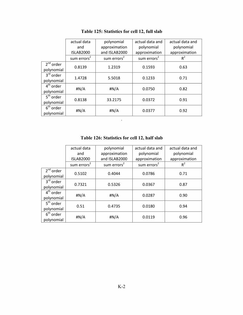
K-2
Table 125: Statistics for cell 12, full slab
actual data and
ISLAB2000
polynomial approximation and ISLAB2000
actual data and polynomial
approximation
actual data and polynomial
approximation
sum errors2 sum errors2 sum errors2 R2
2nd order polynomial
0.8139 1.2319 0.1593 0.63
3rd order polynomial
1.4728 5.5018 0.1233 0.71
4th order polynomial
#N/A #N/A 0.0750 0.82
5th order polynomial
0.8138 33.2175 0.0372 0.91
6th order polynomial
#N/A #N/A 0.0377 0.92
.
Table 126: Statistics for cell 12, half slab
actual data and
ISLAB2000
polynomial approximation and ISLAB2000
actual data and polynomial
approximation
actual data and polynomial
approximation
sum errors2 sum errors2 sum errors2 R2
2nd order polynomial
0.5102 0.4044 0.0786 0.71
3rd order polynomial
0.7321 0.5326 0.0367 0.87
4th order polynomial
#N/A #N/A 0.0287 0.90
5th order polynomial
0.51 0.4735 0.0180 0.94
6th order polynomial
#N/A #N/A 0.0119 0.96
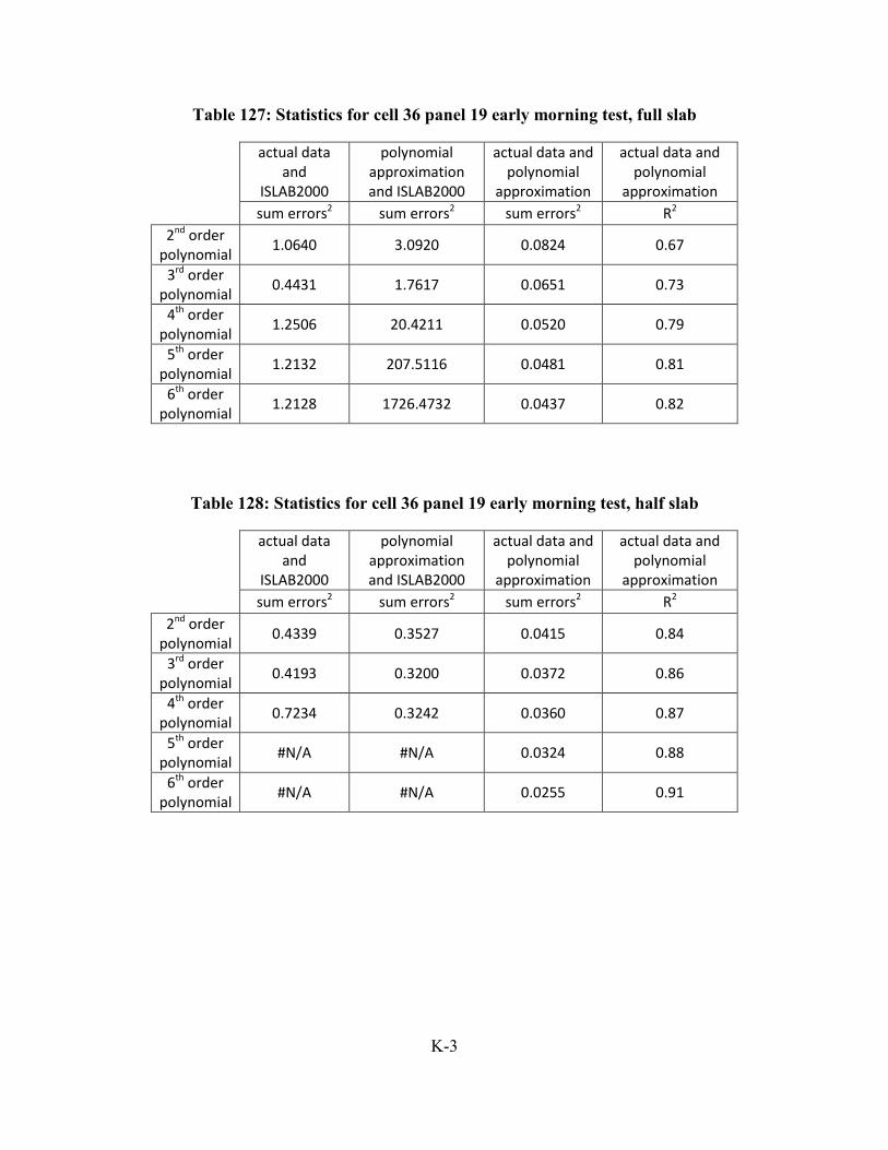
K-3
Table 127: Statistics for cell 36 panel 19 early morning test, full slab
actual data and
ISLAB2000
polynomial approximation and ISLAB2000
actual data and polynomial
approximation
actual data and polynomial
approximation
sum errors2 sum errors2 sum errors2 R2
2nd order polynomial
1.0640 3.0920 0.0824 0.67
3rd order polynomial
0.4431 1.7617 0.0651 0.73
4th order polynomial
1.2506 20.4211 0.0520 0.79
5th order polynomial
1.2132 207.5116 0.0481 0.81
6th order polynomial
1.2128 1726.4732 0.0437 0.82
Table 128: Statistics for cell 36 panel 19 early morning test, half slab
actual data and
ISLAB2000
polynomial approximation and ISLAB2000
actual data and polynomial
approximation
actual data and polynomial
approximation
sum errors2 sum errors2 sum errors2 R2
2nd order polynomial
0.4339 0.3527 0.0415 0.84
3rd order polynomial
0.4193 0.3200 0.0372 0.86
4th order polynomial
0.7234 0.3242 0.0360 0.87
5th order polynomial
#N/A #N/A 0.0324 0.88
6th order polynomial
#N/A #N/A 0.0255 0.91

K-4
Table 129: Statistics for cell 36 panel 19 late morning test, full slab
actual data and
ISLAB2000
polynomial approximation and ISLAB2000
actual data and polynomial
approximation
actual data and polynomial
approximation
sum errors2 sum errors2 sum errors2 R2
2nd order polynomial
2.5965 5.5600 1.4143 0.30
3rd order polynomial
3.4444 47.6606 0.4481 0.76
4th order polynomial
2.1828 108.2365 0.5220 0.74
5th order polynomial
#N/A #N/A 3.9495 0.05
6th order polynomial
#N/A #N/A 3.0009 0.23
Table 130: Statistics for cell 36 panel 19 late morning test, half slab
actual data and
ISLAB2000
polynomial approximation and ISLAB2000
actual data and polynomial
approximation
actual data and polynomial
approximation
sum errors2 sum errors2 sum errors2 R2
2nd order polynomial
1.2585 1.0918 0.3861 0.62
3rd order polynomial
1.6016 1.0527 0.3130 0.69
4th order polynomial
3.3060 1.5443 0.2300 0.78
5th order polynomial
1.2711 1.5050 0.1685 0.84
6th order polynomial
1.4023 2.0043 0.1441 0.86

K-5
Table 131: Statistics for cell 36 panel 20 early morning test, full slab
actual data and
ISLAB2000
polynomial approximation and ISLAB2000
actual data and polynomial
approximation
actual data and polynomial
approximation
sum errors2 sum errors2 sum errors2 R2
2nd order polynomial
0.4281 0.7171 0.1089 0.90
3rd order polynomial
0.4226 3.2348 0.0762 0.96
4th order polynomial
#N/A #N/A 0.0750 0.96
5th order polynomial
#N/A #N/A 0.0822 0.96
6th order polynomial
#N/A #N/A 0.0817 0.97
Table 132: Statistics for cell 36 panel 20 early morning test, half slab
actual data and
ISLAB2000
polynomial approximation and ISLAB2000
actual data and polynomial
approximation
actual data and polynomial
approximation
sum errors2 sum errors2 sum errors2 R2
2nd order polynomial
0.1957 0.1248 0.0359 0.48
3rd order polynomial
0.1758 0.0934 0.0344 0.52
4th order polynomial
#N/A #N/A 0.0298 0.58
5th order polynomial
#N/A #N/A 0.0264 0.61
6th order polynomial
#N/A #N/A 0.0232 0.64
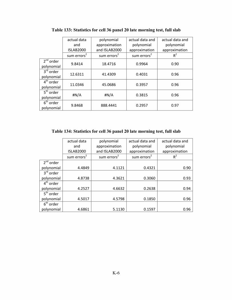
K-6
Table 133: Statistics for cell 36 panel 20 late morning test, full slab
actual data and
ISLAB2000
polynomial approximation and ISLAB2000
actual data and polynomial
approximation
actual data and polynomial
approximation
sum errors2 sum errors2 sum errors2 R2
2nd order polynomial
9.8414 18.4716 0.9964 0.90
3rd order polynomial
12.6311 41.4309 0.4031 0.96
4th order polynomial
11.0346 45.0686 0.3957 0.96
5th order polynomial
#N/A #N/A 0.3815 0.96
6th order polynomial
9.8468 888.4441 0.2957 0.97
Table 134: Statistics for cell 36 panel 20 late morning test, full slab
actual data and
ISLAB2000
polynomial approximation and ISLAB2000
actual data and polynomial
approximation
actual data and polynomial
approximation
sum errors2 sum errors2 sum errors2 R2
2nd order polynomial 4.4849 4.1121 0.4321 0.90
3rd order polynomial 4.8738 4.3621 0.3060 0.93
4th order polynomial 4.2527 4.6632 0.2638 0.94
5th order polynomial 4.5017 4.5798 0.1850 0.96
6th order polynomial 4.6861 5.1130 0.1597 0.96
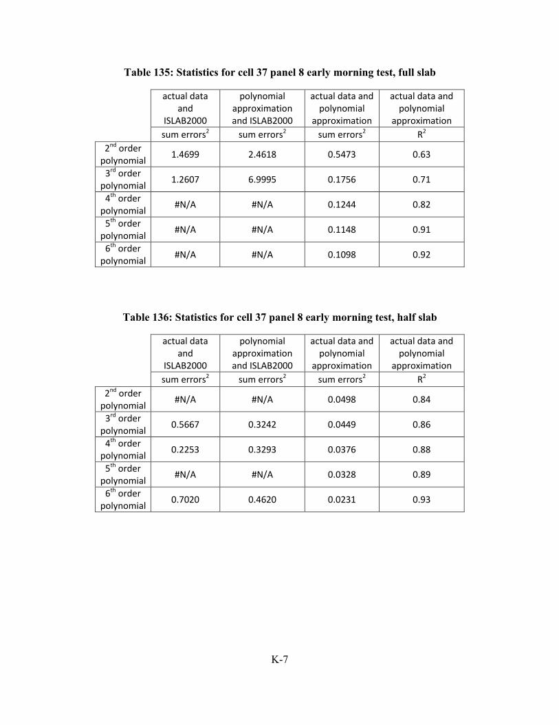
K-7
Table 135: Statistics for cell 37 panel 8 early morning test, full slab
actual data and
ISLAB2000
polynomial approximation and ISLAB2000
actual data and polynomial
approximation
actual data and polynomial
approximation
sum errors2 sum errors2 sum errors2 R2
2nd order polynomial
1.4699 2.4618 0.5473 0.63
3rd order polynomial
1.2607 6.9995 0.1756 0.71
4th order polynomial
#N/A #N/A 0.1244 0.82
5th order polynomial
#N/A #N/A 0.1148 0.91
6th order polynomial
#N/A #N/A 0.1098 0.92
Table 136: Statistics for cell 37 panel 8 early morning test, half slab
actual data and
ISLAB2000
polynomial approximation and ISLAB2000
actual data and polynomial
approximation
actual data and polynomial
approximation
sum errors2 sum errors2 sum errors2 R2
2nd order polynomial
#N/A #N/A 0.0498 0.84
3rd order polynomial
0.5667 0.3242 0.0449 0.86
4th order polynomial
0.2253 0.3293 0.0376 0.88
5th order polynomial
#N/A #N/A 0.0328 0.89
6th order polynomial
0.7020 0.4620 0.0231 0.93

K-8
Table 137: Statistics for cell 37 panel 8 late morning test, full slab
actual data and
ISLAB2000
polynomial approximation and ISLAB2000
actual data and polynomial
approximation
actual data and polynomial
approximation
sum errors2 sum errors2 sum errors2 R2
2nd order polynomial
1.6694 3.2665 0.7941 0.63
3rd order polynomial
2.9838 11.4644 0.7677 0.71
4th order polynomial
1.9923 52.9709 0.6425 0.82
5th order polynomial
#N/A #N/A 0.3003 0.91
6th order polynomial
#N/A #N/A 0.2647 0.92
Table 138: Statistics for cell 37 panel 8 late morning test, half slab
actual data and
ISLAB2000
polynomial approximation and ISLAB2000
actual data and polynomial
approximation
actual data and polynomial
approximation
sum errors2 sum errors2 sum errors2 R2
2nd order polynomial
1.1413 0.6468 0.3488 0.49
3rd order polynomial
1.3235 0.6143 0.2881 0.58
4th order polynomial
#N/A #N/A 0.1904 0.72
5th order polynomial
#N/A #N/A 0.1852 0.73
6th order polynomial
#N/A #N/A 0.1638 0.76
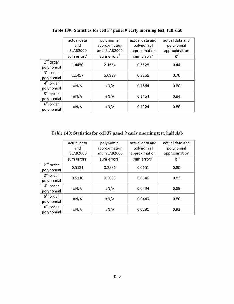
K-9
Table 139: Statistics for cell 37 panel 9 early morning test, full slab
actual data and
ISLAB2000
polynomial approximation and ISLAB2000
actual data and polynomial
approximation
actual data and polynomial
approximation
sum errors2 sum errors2 sum errors2 R2
2nd order polynomial
1.4450 2.1664 0.5528 0.44
3rd order polynomial
1.1457 5.6929 0.2256 0.76
4th order polynomial
#N/A #N/A 0.1864 0.80
5th order polynomial
#N/A #N/A 0.1454 0.84
6th order polynomial
#N/A #N/A 0.1324 0.86
Table 140: Statistics for cell 37 panel 9 early morning test, half slab
actual data and
ISLAB2000
polynomial approximation and ISLAB2000
actual data and polynomial
approximation
actual data and polynomial
approximation
sum errors2 sum errors2 sum errors2 R2
2nd order polynomial
0.5131 0.2886 0.0651 0.80
3rd order polynomial
0.5110 0.3095 0.0546 0.83
4th order polynomial
#N/A #N/A 0.0494 0.85
5th order polynomial
#N/A #N/A 0.0449 0.86
6th order polynomial
#N/A #N/A 0.0291 0.92
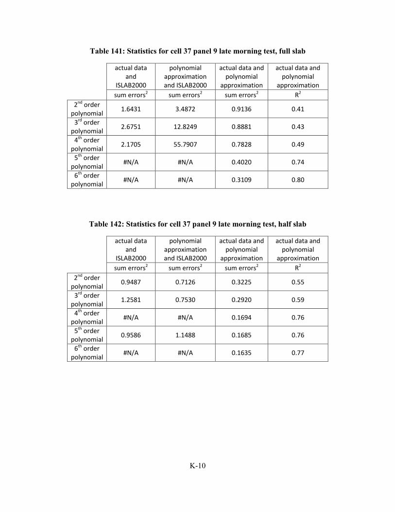
K-10
Table 141: Statistics for cell 37 panel 9 late morning test, full slab
actual data and
ISLAB2000
polynomial approximation and ISLAB2000
actual data and polynomial
approximation
actual data and polynomial
approximation
sum errors2 sum errors2 sum errors2 R2
2nd order polynomial
1.6431 3.4872 0.9136 0.41
3rd order polynomial
2.6751 12.8249 0.8881 0.43
4th order polynomial
2.1705 55.7907 0.7828 0.49
5th order polynomial
#N/A #N/A 0.4020 0.74
6th order polynomial
#N/A #N/A 0.3109 0.80
Table 142: Statistics for cell 37 panel 9 late morning test, half slab
actual data and
ISLAB2000
polynomial approximation and ISLAB2000
actual data and polynomial
approximation
actual data and polynomial
approximation
sum errors2 sum errors2 sum errors2 R2
2nd order polynomial
0.9487 0.7126 0.3225 0.55
3rd order polynomial
1.2581 0.7530 0.2920 0.59
4th order polynomial
#N/A #N/A 0.1694 0.76
5th order polynomial
0.9586 1.1488 0.1685 0.76
6th order polynomial
#N/A #N/A 0.1635 0.77

K-11
Table 143: Statistics for cell 53 early morning test, full slab
actual data and
ISLAB2000
polynomial approximation and ISLAB2000
actual data and polynomial
approximation
actual data and polynomial
approximation
sum errors2 sum errors2 sum errors2 R2
2nd order polynomial
#N/A #N/A 0.3475 0.34
3rd order polynomial
1.2075 2.4964 0.3303 0.36
4th order polynomial
#N/A #N/A 0.2683 0.46
5th order polynomial
#N/A #N/A 0.2349 0.54
6th order polynomial
#N/A #N/A 0.2153 0.60
Table 144: Statistics for cell 53 early morning test, half slab
actual data and
ISLAB2000
polynomial approximation and ISLAB2000
actual data and polynomial
approximation
actual data and polynomial
approximation
sum errors2 sum errors2 sum errors2 R2
2nd order polynomial
#N/A #N/A 0.1171 0.35
3rd order polynomial
0.3551 0.1061 0.1078 0.40
4th order polynomial
#N/A #N/A 0.0636 0.65
5th order polynomial
#N/A #N/A 0.0561 0.70
6th order polynomial
#N/A #N/A 0.0502 0.73

K-12
Table 145: Statistics for cell 53 late morning test, full slab
actual data and
ISLAB2000
polynomial approximation and ISLAB2000
actual data and polynomial
approximation
actual data and polynomial
approximation
sum errors2 sum errors2 sum errors2 R2
2nd order polynomial
#N/A #N/A 0.4695 0.63
3rd order polynomial
1.4423 3.1761 0.4525 0.71
4th order polynomial
1.4173 38.2854 0.2865 0.82
5th order polynomial
#N/A #N/A 0.2605 0.91
6th order polynomial
1.4271 747.5115 0.2189 0.92
Table 146: Statistics for cell 53 late morning test, half slab
actual data and
ISLAB2000
polynomial approximation and ISLAB2000
actual data and polynomial
approximation
actual data and polynomial
approximation
sum errors2 sum errors2 sum errors2 R2
2nd order polynomial
#N/A #N/A 0.1002 0.61
3rd order polynomial
0.4500 0.2223 0.0858 0.67
4th order polynomial
#N/A #N/A 0.0525 0.79
5th order polynomial
#N/A #N/A 0.0465 0.81
6th order polynomial
#N/A #N/A 0.0431 0.82

K-13
Table 147: Statistics for cell 71, full slab
actual data and
ISLAB2000
polynomial approximation and ISLAB2000
actual data and polynomial
approximation
actual data and polynomial
approximation
sum errors2 sum errors2 sum errors2 R2
2nd order polynomial
0.4507 1.7956 0.1842 0.67
3rd order polynomial
0.6750 4.9723 0.0544 0.90
4th order polynomial
#N/A #N/A 0.0500 0.91
5th order polynomial
0.4498 6.5895 0.0376 0.93
6th order polynomial
0.6714 10.5830 0.0315 0.94
Table 148: Statistics for cell 71, half slab
actual data and
ISLAB2000
polynomial approximation and ISLAB2000
actual data and polynomial
approximation
actual data and polynomial
approximation
sum errors2 sum errors2 sum errors2 R2
2nd order polynomial
1.0919 0.5513 0.0837 0.78
3rd order polynomial
0.4004 0.4478 0.0303 0.92
4th order polynomial
#N/A #N/A 0.0139 0.96
5th order polynomial
#N/A #N/A 0.0137 0.96
6th order polynomial
0.4010 0.3794 0.0116 0.97

K-14
Table 149: Statistics for cell 72, full slab
actual data and
ISLAB2000
polynomial approximation and ISLAB2000
actual data and polynomial
approximation
actual data and polynomial
approximation
sum errors2 sum errors2 sum errors2 R2
2nd order polynomial
3.7599 5.5453 0.2383 0.79
3rd order polynomial
4.0126 7.3104 0.1601 0.86
4th order polynomial
3.8222 6.9642 0.1606 0.86
5th order polynomial
#N/A #N/A 0.1629 0.87
6th order polynomial
#N/A #N/A 0.1878 0.85
Table 150: Statistics for cell 72, half slab
actual data and
ISLAB2000
polynomial approximation and ISLAB2000
actual data and polynomial
approximation
actual data and polynomial
approximation
sum errors2 sum errors2 sum errors2 R2
2nd order polynomial
1.3689 0.4599 0.1005 0.60
3rd order polynomial
1.5244 0.2905 0.0942 0.63
4th order polynomial
#N/A #N/A 0.0863 0.65
5th order polynomial
#N/A #N/A 0.0832 0.66
6th order polynomial
#N/A #N/A 0.0671 0.73
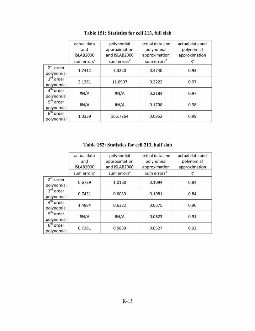
K-15
Table 151: Statistics for cell 213, full slab
actual data and
ISLAB2000
polynomial approximation and ISLAB2000
actual data and polynomial
approximation
actual data and polynomial
approximation
sum errors2 sum errors2 sum errors2 R2
2nd order polynomial
1.7412 3.3220 0.4740 0.93
3rd order polynomial
2.1261 11.0907 0.2222 0.97
4th order polynomial
#N/A #N/A 0.2184 0.97
5th order polynomial
#N/A #N/A 0.1798 0.98
6th order polynomial
1.0339 165.7264 0.0852 0.99
Table 152: Statistics for cell 213, half slab
actual data and
ISLAB2000
polynomial approximation and ISLAB2000
actual data and polynomial
approximation
actual data and polynomial
approximation
sum errors2 sum errors2 sum errors2 R2
2nd order polynomial
0.6729 1.0160 0.1094 0.84
3rd order polynomial
0.7431 0.6033 0.1081 0.84
4th order polynomial
1.4884 0.6322 0.0675 0.90
5th order polynomial
#N/A #N/A 0.0623 0.91
6th order polynomial
0.7281 0.5839 0.0527 0.92

K-16
Table 153: Statistics for cell 305, full slab
actual data and
ISLAB2000
polynomial approximation and ISLAB2000
actual data and polynomial
approximation
actual data and polynomial
approximation
sum errors2 sum errors2 sum errors2 R2
2nd order polynomial
2.6999 7.0880 0.8214 0.81
3rd order polynomial
6.5728 29.5891 0.2054 0.95
4th order polynomial
#N/A #N/A 0.1093 0.97
5th order polynomial
#N/A #N/A 0.0936 0.98
6th order polynomial
4.5964 46.1113 0.0930 0.98
Table 154: Statistics for cell 305, half slab
actual data and
ISLAB2000
polynomial approximation and ISLAB2000
actual data and polynomial
approximation
actual data and polynomial
approximation
sum errors2 sum errors2 sum errors2 R2
2nd order polynomial
0.8168 2.3238 0.0458 0.94
3rd order polynomial
0.9511 1.1315 0.0317 0.96
4th order polynomial
1.5071 1.1194 0.0302 0.96
5th order polynomial
0.8837 1.0173 0.0218 0.97
6th order polynomial
0.8193 0.9254 0.0178 0.98

K-17
Table 155: Statistics for cell 513, full slab
actual data and
ISLAB2000
polynomial approximation and ISLAB2000
actual data and polynomial
approximation
actual data and polynomial
approximation
sum errors2 sum errors2 sum errors2 R2
2nd order polynomial
0.9804 3.3769 0.3291 0.80
3rd order polynomial
2.0992 11.8966 0.1468 0.91
4th order polynomial
#N/A #N/A 0.1395 0.92
5th order polynomial
#N/A #N/A 0.2652 0.88
6th order polynomial
0.9810 81.6861 0.1194 0.94
Table 156: Statistics for cell 513, half slab
actual data and
ISLAB2000
polynomial approximation and ISLAB2000
actual data and polynomial
approximation
actual data and polynomial
approximation
sum errors2 sum errors2 sum errors2 R2
2nd order polynomial
0.6065 0.9145 0.0544 0.91
3rd order polynomial
0.6241 0.6575 0.0479 0.92
4th order polynomial
2.8170 0.6579 0.0251 0.96
5th order polynomial
#N/A #N/A 0.0246 0.96
6th order polynomial
0.5999 0.5736 0.0234 0.96

K-18
Table 157: Statistics for cell 614, full slab
actual data and
ISLAB2000
polynomial approximation and ISLAB2000
actual data and polynomial
approximation
actual data and polynomial
approximation
sum errors2 sum errors2 sum errors2 R2
2nd order polynomial
#N/A #N/A 1.7159 0.63
3rd order polynomial
2.9723 27.5810 3.2966 0.71
4th order polynomial
#N/A #N/A 8.6497 0.69
5th order polynomial
#N/A #N/A 15.9252 0.38
6th order polynomial
2.5226 1929.8181 46.8480 0.74
Table 158: Statistics for cell 614, half slab
actual data and
ISLAB2000
polynomial approximation and ISLAB2000
actual data and polynomial
approximation
actual data and polynomial
approximation
sum errors2 sum errors2 sum errors2 R2
2nd order polynomial
0.7822 0.8042 0.0887 0.88
3rd order polynomial
0.7963 0.7327 0.0747 0.89
4th order polynomial
1.2572 0.7236 0.0616 0.91
5th order polynomial
#N/A #N/A 0.0553 0.92
6th order polynomial
0.7885 0.7216 0.0493 0.92
Related Documents