Field and Numerical Study for Deteriorating Precast Double ...

South Dakota State University South Dakota State University

Open PRAIRIE: Open Public Research Access Institutional Open PRAIRIE: Open Public Research Access Institutional

Repository and Information Exchange Repository and Information Exchange

Electronic Theses and Dissertations

2019

Field and Numerical Study for Deteriorating Precast Double-Tee Field and Numerical Study for Deteriorating Precast Double-Tee

Girder Bridges Girder Bridges

Brian Kidd South Dakota State University

Follow this and additional works at: https://openprairie.sdstate.edu/etd

Part of the Civil Engineering Commons, Structural Engineering Commons, and the Transportation

Engineering Commons

Recommended Citation Recommended Citation Kidd, Brian, "Field and Numerical Study for Deteriorating Precast Double-Tee Girder Bridges" (2019). Electronic Theses and Dissertations. 3631. https://openprairie.sdstate.edu/etd/3631

This Thesis - Open Access is brought to you for free and open access by Open PRAIRIE: Open Public Research Access Institutional Repository and Information Exchange. It has been accepted for inclusion in Electronic Theses and Dissertations by an authorized administrator of Open PRAIRIE: Open Public Research Access Institutional Repository and Information Exchange. For more information, please contact [email protected].

https://openprairie.sdstate.edu/

https://openprairie.sdstate.edu/

https://openprairie.sdstate.edu/etd

https://openprairie.sdstate.edu/etd?utm_source=openprairie.sdstate.edu%2Fetd%2F3631&utm_medium=PDF&utm_campaign=PDFCoverPages

http://network.bepress.com/hgg/discipline/252?utm_source=openprairie.sdstate.edu%2Fetd%2F3631&utm_medium=PDF&utm_campaign=PDFCoverPages




https://openprairie.sdstate.edu/etd/3631?utm_source=openprairie.sdstate.edu%2Fetd%2F3631&utm_medium=PDF&utm_campaign=PDFCoverPages

mailto:[email protected]

FIELD AND NUMERICAL STUDY FOR DETERIORATING PRECAST

DOUBLE-TEE GIRDER BRIDGES

BY

BRIAN KIDD

A thesis submitted in partial fulfillment of the requirements for the

Master of Science

Major in Civil Engineering

South Dakota State University

2019

ii

THESIS ACCEPTANCE PAGE

This thesis is approved as a creditable and independent investigation by a candidate for

the master’s degree and is acceptable for meeting the thesis requirements for this degree.

Acceptance of this does not imply that the conclusions reached by the candidate are

necessarily the conclusions of the major department.

Advisor Date

Department Head Date

Dean, Graduate School Date

Brian Kidd

Junwon Seo

Nadim Wehbe

iii

ACKNOWLEDGEMENTS

I acknowledge my gratitude to all of the people who helped me along the way.

To my major professor Dr. Junwon Seo, it has been an invaluable experience working

with you and your knowledge. I have learned incredible amounts of information that I

could not have gotten elsewhere. I appreciate you putting your faith, trust, and time

into me. Thank you Dr. Nadim Wehbe, for your guidance and input on my thesis. I

also appreciate the time you spent in class teaching me based on your vast

experiences and knowledge. Thank you Dr. Leda Cempellin for taking the time to be

a part of my graduate committee. Thank you Dr. Tazarv for your guidance and help

on the field testing and analytical modeling. It has been a big help to have great

professors such as you all to guide me and create a wonderful educational experience

for me. Thank you to Mr. Zach Gutzmer and all of the others who have helped me

along the way. To the Mountain Plains Consortium (MPC), USDOT, and South

Dakota State, thank you for the funds dedicated to my research project and my

education. A special thanks to my parents, Tim and Bonnie Kidd, my sister Megan

Kidd, and the rest of my family for encouraging me and supporting me during the

pursuit of my degree.

iv

CONTENTS

ABSTRACT………….......……………………………………………………………x

INTRODUCTION……………………..……………………………………………...1

RESEARCH OBJECTIVES……………………………………………………......…2

SCOPE OF RESEARCH……………………………………………………......…….2

OUTLINE OF THESIS………………………………………………..………………3

CHAPTER 1: FIELD TESTING OF DOUBLE-TEE BRIDGES FOR

DISTRIBUTION FACTORS AND DYNAMIC LOAD ALLOWANCE.……...........4

1.1 ABSTRACT…………………………………………………………………...5

1.2 INTRODUCTION…………………………………………………………….6

1.3 BRIDGE DESCRIPTION AND DETERIORATION…………….…………10

1.3.1 762-MM DEEP DTG BRIDGE……………………....………….10

1.3.2 584-MM DEEP DTG BRIDGE………………………………….13

1.4 FIELD TESTING…………………………………………………………….15

1.4.1 TRUCK CONFIGURATION……………………………………15

1.4.2 TRUCK PATHS………...…………………....………………….16

1.4.3 INSTRUMENTATION PLAN…………………………………..18

1.5 RESULTS AND DISCUSSION......................................................................19

1.5.1 LIVE LOAD DISTRIBUTION FACTORS..................................19

1.5.1.1 MEASURED STRAINS....................................................19

1.5.1.2 LLDF EQUATIONS..........................................................25

1.5.1.3 COMPARISON BETWEEN FIELD AND CODE

CALCULATED LLDFS....................................................27

v

1.5.2 DYNAMIC LOAD ALLOWANCE..............................................34

1.6 CONCLUSIONS.............................................................................................39

1.7 DATA AVAILABILITY.................................................................................40

1.8 ACKNOWLEDGEMENTS.............................................................................40

1.9 REFERENCES................................................................................................42

2 CHAPTER 2: COMPARISON OF DATA-DRIVEN LOAD DISTRIBUTION

DETERMINATION APPROACHES TO PRECEAST PRESTRESSED DOUBLE-

TEE BRIDGES............................................................................................................45

2.1 ABSTRACT.....................................................................................................46

2.2 INTRODUCTION...........................................................................................47

2.3 OVERVIEW OF STUDIED BRIDGES..........................................................50

2.3.1 BRIDGE A.....................................................................................50

2.3.2 BRIDGE B.....................................................................................52

2.4 FIELD TESTING.............................................................................................54

2.5 RESULTS AND DISCUSSION......................................................................57

2.5.1 GIRDER APPROACH..................................................................59

2.5.2 STEM APPROACH......................................................................62

2.5.3 JOINT APPROACH......................................................................67

2.6 SUMMARY AND CONCLUSIONS..............................................................73

2.7 ACKNOWLEDGEMENTS.............................................................................74

2.8 REFERENCES................................................................................................75

3 CHAPTER 3: EFFECT OF DAMAGE ON LIVE-LOAD DISTRIBUTION

FACTORS OF DOUBLE-TEE BRIDGE GIRDERS.................................................77

vi

3.1 ABSTRACT.....................................................................................................78

3.2 INTRODUCTION...........................................................................................79

3.3 BRIDGE DESCRIPTION................................................................................81

3.3.1 Bridge A.........................................................................................81

3.3.2 Bridge B.........................................................................................82

3.4 FIELD TESTING (KIDD ET AL. 2020).........................................................83

3.5 DAMAGE QUANTIFICATION.....................................................................88

3.5.1 BRIDGE INSPECTION................................................................89

3.5.2 DAMAGE TYPE AND PORTION...............................................93

3.5.3 AASHTO BDI AND DAMAGE STATE......................................93

3.5.4 WEIGHTED DAMAGE PORTION AND DAMAGE RATIOS..94

3.6 LLDF DETERMINATION.............................................................................98

3.7 RESULTS AND DISCUSSION....................................................................100

3.7.1 COMPARISON WITH FIELD LLDFS......................................100

3.7.2 COMPARISON WITH AASHTO LLDFS.................................106

3.8 CONCLUSION..............................................................................................110

3.9 ACKNOWLEDGEMENTS...........................................................................111

3.10 REFERENCES........................................................................................113

4 CHAPTER 4: PARAMETRIC STUDY OF DOUBLE-TEE GIRDER BRIDGES

USING LIVE-LOAD DISTRIBUTION FACTORS.................................................115

4.1 ABSTRACT...................................................................................................116

4.2 INTRODUCTION.........................................................................................117

4.3 BRIDGES TESTED.......................................................................................119

vii

4.3.1 BRIDGE A...................................................................................119

4.3.2 BRIDGE B...................................................................................122

4.4 REVIEW OF FIELD TESTS.........................................................................124

4.4.1 FIELD TEST SUMMARY..........................................................124

4.4.2 DATA ANALYSIS......................................................................127

4.5 BRIDGE MODELING..................................................................................132

4.5.1 COMPUTER MODELING.........................................................132

4.5.2 CALIBRATION..........................................................................134

4.6 PARAMETRIC STUDY...............................................................................136

4.7 RESULTS......................................................................................................137

4.7.1 SPAN LENGTH..........................................................................137

4.7.2 LOCATION OF DIAPHRAGMS...............................................142

4.7.3 DECK WIDTH............................................................................146

4.7.4 CONCRETE STRENGTH...........................................................150

4.7.5 WIDTH-LENGTH RATIO..........................................................154

4.8 SUMMARY AND CONCLUSIONS............................................................160

4.9 ACKNOWLEDGEMENTS...........................................................................161

4.10 REFERENCES........................................................................................163

viii

ABSTRACT

FIELD AND NUMERICAL STUDY FOR DETERIORATING PRECAST

DOUBLE-TEE GIRDER BRIDGES

BRIAN KIDD

2019

Two deteriorating DT bridges in South Dakota, both over 30-years old, were

field tested with a static and dynamic load. From the recorded strain values, the live-

load distribution factors (LLDFs) and dynamic load allowance (IM) factors were

calculated. The AASHTO LRFD and AASHTO Standard Specifications were

compared with the field LLDFs and IMs. It was determined that the AASHTO LRFD

Specifications were conservative for deteriorating DT girder bridges, with two

exceptions. The AASHTO Standard codified LLDFs were significantly higher than

the field LLDFs in all cases. The AASHTO LRFD and AASHTO Standard

specifications were conservative when calculating the IM factors in all instances for

the two deteriorating DT bridges.

The strain data from the field tests was analyzed for LLDFs in three different

approaches. Then, these approaches were compared to AASHTO LRFD and

AASHTO Standard specifications. The girder approach had an average percent

difference of 34% and 91% when compared to the AASHTO LRFD and AASHTO

Standard specifications, respectively. The joint approach produced average percent

differences similar to the girder approach. The stem approach was the most

conservative approach, with an average percent difference of 58%, compared to

AASHTO LRFD.

ix

A visual inspection was conducted on both bridges and the damage was

identified using the AASHTO Manual for Bridge Element Inspection. The damage

was organized by a joint damage ratio and then a girder damage ratio. Graphical

comparisons and a simple linear regression compared the damage ratios to the

LLDFs. Both methods suggested that, when the wheel loads were over the joints with

the most damage, the LLDFs were higher.

Finite element models were calibrated with the strain data from the field tests.

The span length, deck width, concrete strength, use of diaphragms, and width-length

ratio was investigated for its effect on the LLDFs. The LLDFs decreased as the span

length increased. The other parameters showed insignificant changes in the LLDFs.

The AASHTO LRFD interior LLDFs were consistent with the analytical LLDFs.

Analytical exterior LLDFs decreased with span length as well, which was not

consistent with AASHTO LRFD exterior LLDFs. The results are discussed herein.

1

INTRODUCTION

South Dakota has been using double-tee (DT) girder bridges for many

years on county road bridges. There are hundreds of DT girder bridges in service. It is

important to understand how damage affects the structural performance of the DT

bridges. Accurate estimation of live load distribution factors (LLDFs) and dynamic

load allowance (IM) for girder bridges, including precast, prestressed DT bridges, is

crucial for a safe design. Bridges with damage may result in the load path changing.

Meaning, if damage is significant enough, the LLDFs and IMs may change

substantially. However, no previous field study has investigated LLDFs and IM for

DTG bridges with significant damage of the longitudinal joints.

The AASHTO Manual for Bridge Element Inspection (AASHTO 2013) is the

basis for categorizing individual bridge components based on its descriptive and

quantitative condition states descripting damage states. The damage states vary from

one to four. One being good condition and four meaning severe damage. However,

this still creates subjective results, as the conditions are selected based upon the

bridge inspector’s evaluation. Hence, more research is needed to quantify damage on

bridges.

The analysis of the deteriorating DT girder bridges was completed using field

tests on two representative bridges and then analytical models can be used to study

the effects of different parameters on the LLDFs. Analytical models are useful tools,

as this saves time and money, instead of field testing more bridges.

2

RESEARCH OBJECTIVES

The main objectives of this study was to understand how the damage on a DT

girder bridge affected the structural performance of the bridge. Specifically, how the

LLDFs and IMs change due to longitudinal joint damage. Field tests were conducted

to determine LLDFs and IMs, inspections were conducted to identify the damage on

the bridges, and finite-element models were created to further investigate the LLDFs.

SCOPE OF RESEARCH

The scope of research is detailed as follows:

• Conduct a literature review on the state-of-the-art on the LLDFs and IMs for DT

girder bridges, including field testing and analytical testing, to gather relevant

techniques and findings.

• Determine the LLDFs and IMs of two deteriorating DT girder bridges using field

test data and compare the field results to the AASHTO LRFD and AASHTO

Standard specifications.

• Investigate alternative approaches to calculating the LLDFs on DT girder bridges.

• Inspect and quantify the longitudinal joint damage between girders. Determine the

relationship between the LLDFs and damage present on the bridge.

• Create analytical models and calibrate them based on field testing results.

Conduct a parametric study on deteriorating DT girder bridges.

3

OUTLINE OF THESIS

This thesis contains four research papers, discussed in four different chapters.

The thesis discusses the investigation of the structural performance of deteriorating

DT girder bridges, including LLDFs and IMs. Chapter one summarizes the field

testing procedures and results for the two representative DT girder bridges and

includes an up to date summary of existing literature. The description of the bridges

tested is also included. Chapter two discusses the strain data from the field tests and

proposes two new approaches to calculating the LLDFs of DT girder bridges. A

literature review on LLDFs and a comparison of the new approaches to the AASHTO

LRFD and AASHTO Standard codified LLDFs is included herein. Chapter three

discusses the longitudinal joint damage present on one DT girder bridge and attempts

to quantify the damage using the AASHTO Manual for Bridge Element Inspection.

Based on the inspection and quantification of damage, a simple statistical analysis

was conducted to study the effects of longitudinal joint damage on the LLDFs.

Chapter four discusses the creation and calibration of a finite element model for both

DT girder bridges using CSi Bridge. The models were then used for a parametric

study on the LLDFs of deteriorating DT girder bridges. Span length, deck width,

concrete compressive strength, diaphragm location, and width-length ratio were all

included in this parametric study.

4

CHAPTER 1: FIELD TESTING OF DOUBLE-TEE BRIDGES FOR

DISTRIBUTION FACTORS AND DYNAMIC LOAD ALLOWANCE

Brian Kidd, EIT, S.M. ASCE

Graduate Research Assistant

Department of Civil and Environmental Engineering


Email: [email protected]

Phone: (507) 456-3065

5

ABSTRACT

This paper discusses the field testing of two single-span double-tee girder

(DTG) bridges in South Dakota to determine live load distribution factors (LLDFs)

and the dynamic load allowance (IM). One bridge had seven girders and another had

eight girders. The longitudinal girder-to-girder joints of both bridges were

deteriorated in a way that water could penetrate and the joint steel members were

corroded. A truck traveled across each of the two bridges at five transverse paths. The

paths were tested twice with a crawl speed load test and twice with a dynamic load.

The LLDFs and IM were determined using strain data measured during the field tests.

These results were compared with those determined according to the AASHTO

Standard and the AASHTO LRFD specifications. Nearly all the measured LLDFs

were below the AASHTO LRFD design LLDFs, with the exception of two instances:

1) An exterior DTG on the seven-girder bridge and 2) An interior DTG on the eight-

girder bridge. The LLDFs specified in the AASHTO Standard were conservative

compared with the measured LLDFs. It was also found that both AASHTO LRFD

and AASHTO Standard specifications were conservative when estimating IM,

compared to the field test results for both bridges.

Key Words: Field testing, double-tee girder bridges, live load distribution factor,

dynamic load allowance, longitudinal joint damage.

6

INTRODUCTION

Understanding how live loads (including dynamic effects) are distributed in

various bridge elements, especially girders, is challenging. Accurate estimation of

live load distribution factors (LLDFs) and dynamic load allowance (IM) for girder

bridges, including precast, prestressed double-tee girder (DTG) bridges, is crucial for

a safe design. If live loads distributed to a girder are not correctly estimated, the

girder may damage and need repair or replacement before reaching the design service

life of the bridge. The determination of LLDFs for aged or distressed bridges is even

more critical and challenging since the damage may change the load path. Safe

estimation of the IM factors are also important for a successful design since they are

to amplify the live loads. Without applying IM factors, the design loads will not

represent actual live loading conditions.

A DTG bridge system has been commonly used on South Dakota local roads

due to their ease of construction and cost effectiveness. DTGs are placed side-by-side

on the abutments, a welded steel plate connection is used to discretely connect the

girders (usually at a distance of 1.5 m), and the girder-to-girder keyway is filled

onsite with a non-shrink grouted. Previous studies (Wehbe et al., 2016; Tazarv et al.,

2019) have demonstrated that this joint detailing is not sufficient for service and

strength limit states and proposed new detailing or rehabilitation techniques to

improve the DTG longitudinal joint performance. Damage of DTG longitudinal joints

is especially important in this study since this damage type affects the live load

7

distribution between the girders. No previous field study has investigated LLDFs and

IM for DTG bridges with significant damage of the longitudinal joints.

However, the estimation of LLDFs are not a new topic for the other bridge

types (Zokaie, 2000). The AASHTO Standard Specifications for Highway Bridges

(AASHTO Standard, 1996) has included equations (entitled as “S-over” equations)

for LLDFs since 1931. The past study led by Zokaie (2000) concluded that these

equations were accurate only for common bridges (e.g., bridges with approximately

1.8 m girder spacing and a span length of 18 m) and deviated for short and long

bridges. The AASHTO LRFD Bridge Design Specifications (AASHTO LRFD, 2012)

modified those equations for the determination of LLDFs for interior and exterior

girders in 1994. Compared with AASHTO Standard, the AASHTO LRFD equations

included more bridge types and more variables to determine LLDFs. Some of these

variables include spacing, span length, and longitudinal stiffness. It was reported that

the AASHTO Standard and LRFD equations were developed based on studies that

did not specifically include DTG bridges (PCINE, 2012).

Many studies (Yousif and Hindi, 2007; Hodson et al., 2012; Seo and Hu,

2014; Seo et al., 2014a,b; Seo and Hu, 2015; Seo et al., 2017) have attempted to

estimate LLDFs of different types of bridges loaded with varying trucks or atypical

vehicles and to compare them against the design LLDFs. For instance, Yousif and

Hindi (2007) compared the AASHTO LRFD LLDFs with a finite element model

(FEM) of prestressed I-girder bridges. The study reported that the AASHTO LRFD

8

LLDFs were sometimes over- and under-conservative with different girder spacing,

span length, and slab thickness. Torres (2016) determined through field testing that

the AASHTO LRFD flexural LLDFs provided estimations consistent with that of a

DTG bridge with significantly deteriorated DTG flanges, implying it may be

conservative for DTG bridges without damage. Kim and Nowak (1997) also

concluded that measured LLDFs are consistently lower than those of the AASHTO

methods. Through field testing, Hodson et al. (2012) found that the AASHTO LRFD

LLDFs were conservative for interior posttensioned box girders but slightly under-

conservative for exterior box girders. The LLDFs calculated according to AASHTO

LRFD may not be representative of bridges with atypical vehicles traveling over them

(Seo and Hu, 2014; Seo et al., 2014a, b; Seo and Hu, 2015; Seo et al., 2017). It was

found that uncommon vehicle configurations such as husbandry vehicles, can cause

LLDFs that are higher than the AASHTO LRFD values.

A few analytical studies determined LLDFs for DTG bridges. Finite element

models (FEMs) were developed for DTG bridges using shell and link elements

(Singh, 2012; Torres, 2016). Singh (2012) found that flexural LLDFs decrease as the

DTG span length increases, which is in agreement with the AASHTO LRFD

equations for LLDFs. Torres (2016) was able to correctly model a DTG bridge with

deteriorated flanges in SAP2000 by using link elements to simulate the transverse

load distribution. Huang and Davis (2017) used the PCI (2003) method to estimate

flexural LLDFs. PCI (2003) suggests treating every stem as an independent girder,

then using the LLDF equation for a concrete I-girder bridge from the AASHTO

9

LRFD by utilizing the average spacing between all the stems. The result is then

doubled to represent a full DTG, but this method overestimates the LLDFs.

IM factors take into account the dynamic effect of a moving vehicle. When a

vehicle drives over the bridge, the suspension system of the vehicle creates a dynamic

effect, causing the load from the vehicle to be greater than the static load of the

vehicle. IM is a factor of the span length, bridge stiffness, road surface condition,

vehicle speed, and the vehicle suspension system. Deng et al. (2014) conducted a

state-of-the-art review and found that the IM increases as the span length decreases

and increases as the road surface condition worsens. AASHTO Standard (1996) and

PCI (2003) include an equation for IM based on the span length, but sets a maximum

of 30%. AASHTO LRFD (2012) specifies a constant value of 33% for the dynamic

load allowance for ordinary bridges. Codes in other countries typically use the span

length in determination of IMs. However, there are still some discrepancies in

previous studies, specifically, whether the characteristics of truck affect IM. For

example, Deng et al. (2014) concluded that IM is independent of the number of

vehicle axles, and Ashebo et al. (2007) reported that IM decreases as the weight of

the vehicle increases. Kim and Nowak (1997) concluded that IM factors decrease as

the static strain increases and that measured IM factors for large static strains are well

below those of the AASHTO specifications.

The main goal of this study was to determine LLDFs and IMs for two DTG

bridges with damaged girder-to-girder joints through field testing. To accomplish this

10

goal, one truck was used to perform static and dynamic field tests. Surface-mount

strain gauges were placed at the bottom of each stem at the mid-span of each of the

bridges to measure the strain induced by the truck. The measured data was used to

determine the actual LLDFs and IMs. These values were then compared with those

from AASHTO LRFD and AASHTO Standard. The bridge description and

deterioration, and the field test program are summarized, and the results are discussed

in the following sections.

BRIDGE DESCRIPTION AND DETERIORATION

762-mm Deep DTG Bridge

The first field testing was carried out on a single–span bridge, consisting of

seven 762-mm deep prestressed double-tee girders, on a gravel road. This DTG is one

of the standard sections used for DTG bridges in South Dakota, the cross section is

show later in the paper. The bridge span length was 11.6 meters. The bridge, which

was located in Lincoln County in South Dakota, was 34 years old at the time of

testing. Each of the girders supported by concrete abutments was 1.2 m wide, and had

a zero degree skew angle. The girders were longitudinally connected using a steel

plate connection and grouted shear key. Figures 1a and 1b show the road surface and

bridge underneath, respectively. Figure 2 shows the damage map of the 762-mm deep

DTG bridge observed before the field testing. The main bridge damage was the

deterioration of the girder-to-girder joints including leakage between joints,

efflorescence, and corrosion of steel plates. Figure 3 shows an example of

11

efflorescence on the 762-mm deep girder bridge. Small spalling was also observed for

some of the girder stems.

a) View of bridge from the road

surface

b) View from bridge underneath

FIGURE 1. Description of 762-mm Deep DTG Bridge

12

FIGURE 2. Damage Map of 762-mm Deep DTG Bridge

FIGURE 3. Example of Efflorescence on 762-mm Deep DTG Bridge

13

584-mm Deep DTG Bridge

The second field testing was performed on another single-span, prestressed

DTG bridge but incorporating eight 584-mm deep girders. The bridge span length

was 15.24 m, and the bridge was simply supported on timber abutments, with no

skew angle. At the time of testing, this bridge had been in-service for 38 years in

Moody County in South Dakota. This is one of the standard DTG sections used in

South Dakota DTG bridges. The cross section is shown later in this paper. The bridge

has a gravel wearing surface. Each girder was 1.17-m wide connected to the adjacent

girder using a steel-plate connection and grouted joint. Figure 4 shows the road

surface and a view from the bridge underneath. A visual inspection was conducted

before the field tests, and Fig. 5 shows the observed damage including the

efflorescence and water leakage in the girder-to-girder joints. An example of the

leakage is shown in Figure 6.

a) View of bridge from road surface b) View from bridge underneath

FIGURE 4. Description of 584-mm Deep DTG Bridge

14

FIGURE 5. Damage Map of 584-mm Deep DTG Bridge

FIGURE 6. Example of Efflorescence on 584-mm Deep DTG Bridge

15

FIELD TESTING

The research team conducted field tests on the two DTG bridges. Each bridge

was tested with static and dynamic loads using one truck. Details on the field testing

are presented herein.

Truck Configuration

As shown in Figure 7, the truck used for all the field tests was a South Dakota

Legal Type 3 Truck. The truck weighed 222 kN, with a front axle weight of 74.6 kN

and a combined weight of 147.7 kN for the rear two axles. The weight per each rear

axle was not measured. The axle configuration can be seen in Figure 8. The distance

between the first and second axle was 4.97 m. The distance between the rear two

axles was approximately 1.5 m.

FIGURE 7. South Dakota Legal Load Type 3 Truck used for Field Testing

16

FIGURE 8. Axle Configuration for the Field Testing Truck

Truck Paths

Both static and dynamic load tests using the legal type 3 truck were performed

on each bridge. The goal of the static load tests was to examine the flexural LLDFs of

the DTG bridges at the midspan, while the dynamic testing was intended to compare

the dynamic response with the static response, to calculate IMs.

Figures 9 and 10 show the truck paths for the two bridges. As part of the static

load tests, the truck followed the paths at a crawl speed of 8 km/h. Note that the

exterior paths (A and E) were offset by 0.61 m from the edge of the exterior girder.

The paths were chosen such that the truck axles would directly load two girders at a

time, and all girders would be loaded at least once throughout the field testing.

17

FIGURE 9. 762-mm Deep DTG Bridge Truck Passes for Field Testing

FIGURE 10. 584-mm Deep DTG Bridge Truck Passes for Field Testing

18

Each path was tested twice with the same truck. The dynamic load, which was

done by passing the truck with a speed of 56 km/h, was carried out only for the three

interior paths, Path B through Path D. This was done for the safety of the driver and

the crew when working on a narrow gravel road. The gravel road was narrower than

the bridge.

Instrumentation Plan

Figure 11 shows the field test instrumentation plan for the two bridges. The

girder strains were collected using surface-mounted strain gauges. For the 762-mm

deep DTG bridge, one strain gauges was installed on each stem of all the girders at

the bridge midspan, totaling 14 sensors. The strain was measured over a 305-mm

length as recommended by the sensor manufacturer for concrete bridges. The same

instrumentation plan was used for the 584-mm deep DTG bridge. Due to the stem

damage, strain gauges could not be placed at the bottom faces of a few stems. In those

cases, the strain sensors were placed on the side of the girder, as close as possible to

the bottom. Figure 12 shows an example of two strain gauges installed on girders at

the midspan.

19

a) 762-mm Deep DTG Bridge b) 584-mm Deep DTG Bridge

FIGURE 11. Location of Strain Gauges on both Bridges Tested

FIGURE 12. Example of Strain Transducers Mounted at the Bottom of Stems

RESULTS AND DISCUSSION

Live Load Distribution Factors (LLDFs)

Measured Strains

Figures 13 shows the measured strains over the length of the 782-mm deep

DTG bridge under the static loading. Note that the data for path A on the 782-mm

deep DTG bridge was lost when transferring from the data logger. Under the Path B

loading, Girder G3 exhibited the highest strain (Fig. 13a). Girders G4 and G2, which

20

were directly underneath the wheel paths, had the next highest strains. The strains for

other girders were significantly lower since the load was farther away. The same

trend was observed for other interior load paths. Figure 13d shows the measured

strains for Path E loading, which was on an exterior girder. It can be seen that the

exterior girder had significantly larger strains than the other girders (i.e. 350

microstrain compared to 250 microstrain). Furthermore, Fig. 13 shows that the three

girders underneath the load had significantly higher strain values than the remaining

girders. The maximum strains measured in the 762-mm deep DTG bridge were in a

ranging of 200 to 350 microstrain. Note, the highest strain was measured in Girder 7

under the Path E loading (Fig. 13d) and the lowest stains were seen in the girders

under Path D loading (Fig. 13c).

a) Path B

G3

G4

G2

21

b) Path C

c) Path D

22

Path E

FIGURE 13. Strain versus Location of the Front Axle of Truck for 762-mm Deep

DTG

Bridge

Figure 14 shows the measured strains over the length of the 584-mm deep

DTG bridge under the static loading. Figures 14a-e show the response for the 584-

mm deep DTG bridge. Figures 14a and 14e show the response caused by loaded

exterior girders, resulting in high strain values for the exterior girders, G1 and G8

respectively. Figure 14c shows G3, G4 and G5 as the largest strain values, which are

directly underneath the load. A similar trend is shown in all the strain response

figures for the 584-mm deep DTG bridge. However, Figure 14b shows that G5 has a

similar strain value to G3, even though G3 is underneath the load. This shows that

more of the truck load was distributed transversely. The 584-mm deep DTG bridge

had maximum strain values ranging from 600 – 1100 microstrain from field tests as

shown in Figure 14a for the smallest strain and in Figure 14e for the largest strain.

23

a) Path A

b) Path B

24

c) Path C

d) Path D

25

e) Path E

FIGURE 14. Strain versus Location of the Front Axle of Truck for 584-mm Deep

DTG Bridge

LLDF Equations

The peak strain values induced by the truck were used for the determination of the

LLDFs for the girders. The average strain of the two stems for each girder was

reported as the strain per girder. The commonly used equation below (as used by Seo

et al., 2014a) can be used for calculating LLDFs from the field strain.

�� ∑ �� (1)

where, εi is the field test measured strain for each girder of the bridge. The field

LLDFs calculated according to Eq. 1 were compared with those from AASHTO

LRFD and AASHTO Standard.

26

According to AASHTO LRFD, LLDFs for a DTG can be estimated using Eq.

2, which was for an interior girder with one lane loaded. Note, this equation is

empirical in accordance with U.S. customary units. The data was collected in U.S.

customary units, therefore this equation was used.

�� 0.06 + � ��.� ��

��.� � ��.�

(2)

where, S is the spacing of the girders (ft), L is the span length (ft), Kg is the

longitudinal stiffness of the girder (in4), and ts is the thickness of the bride deck (in)

[1 ft = 0.3048 m and 1 inch = 25.4 mm]. Note, exterior DTG LLDFs were calculated

using the lever rule (AASHTO LRFD, 2012).

According to AASHTO Standard, equations (3) through (6) can be used to

calculate the LLDFs for both the interior and exterior girders on DTG bridges. Again,

the AASHTO US version was used herein since the data was collected as such.

�� /� (3)

� � �5.75 − 0.5"�# + 0.7"��1 − 0.2&#� (4)

& � ' �(� � (5)

' � )�1 + *# + ,⁄ .�./ (6)

where, S is the girder spacing (ft), NL is the number of lanes, µ is the Poisson’s ratio, I

is the moment of inertia, J is the polar moment of inertia, W is the width of the bridge,

and L is the span length of the bridge (ft). The AASHTO Standard Specifications are

27

outdated, however, since the bridges were designed, at a minimum, thirty years ago,

they were designed according to the AASHTO Standard Specifications. The relation

of the field LLDFs to the design LLDFs is necessary to investigate.

Comparison between Field and Code calculated LLDFs

Figure 15 shows the LLDFs from the field testing of the 762-mm deep DTG bridge

and the code calculated LLDFs according to the AASHTO LRFD and Standard

equations. Furthermore, Table 1 presents the field LLDFs for this bridge.

Table 1. Field LLDFs for 762-mm Deep DTG Bridge

Path G1 G2 G3 G4 G5 G6 G7

Path A* N/A N/A N/A N/A N/A N/A N/A

Path B 0.084 0.270 0.293 0.227 0.079 0.020 0.026

Path C 0.036 0.110 0.282 0.257 0.208 0.071 0.048

Path D 0.018 0.033 0.087 0.209 0.204 0.235 0.214

Path E 0.004 0.021 0.022 0.066 0.141 0.212 0.534

*Data from Path A was lost.

Overall, the field LLDFs were largest for the loaded girders. For example,

under Path C in which the truck was passing though the bridge (e.g. girders G3

through G5 for the 762-mm deep DTG bridge), the middle girders (G3, G4, and G5)

that were under the truck had the highest LLDFs. Table 2 presents a summary of field

and code calculated LLDFs for this bridge. The only instance when the field LLDFs

exceed the AASHTO LRFD values is gird G7. This can be seen in Table 2 on the

next page.

28

Table 2. Comparison of Measured and Specified LLDFs for 762-mm Deep DTG

Bridge

Girder ID Max Measured AASHTO

LRFD

AASHTO

Standard

G1* 0.084 0.52 0.768

G2 0.27 0.38 0.768

G3 0.293 0.38 0.768

G4 0.257 0.38 0.768

G5 0.208 0.38 0.768

G6 0.235 0.38 0.768

G7 0.534 0.52 0.768

*Girder 1 does not have data associated with Path A.

The same trend was also observed in the 584-mm deep DTG bridge as shown

in Fig. 16. The only exception was for girder G5 of the 584-mm deep DTG bridge.

This girder, which was not under the truck, showed the same LLDF as girder G3,

which was between the wheel paths. From the present data, it appears that only the

exterior girder, G7, had a field LLDF that was close to that of AASHTO LRFD. This

may be due to the damage along the longitudinal joint between girders G6 and G7 as

shown in Fig. 2. For other girders, the field LLDFs were least 20% smaller than

those form AASHTO LRFD. Note, LLDF for girder G1 is an outlier because data

from the field tests for Path A was not available. It can be concluded that LLDFs

from AASHTO LRFD and AASHTO Standard for all the girders, excluding girder

G7, were significantly higher than the field LLDFs for this bridge.

29

a) Path B

b) Path C

0.00

0.10

0.20

0.30

0.40

0.50

0.60

0.70

0.80

0.90

1 2 3 4 5 6 7

Dis

trib

uti

on

Fa

cto

r

Girder NumberField AASHTO LRFD AASHTO Standard

0.00

0.10

0.20

0.30

0.40

0.50

0.60

0.70

0.80

0.90

1 2 3 4 5 6 7

Dis

trib

uti

on

Fa

cto

r

Girder Number

Field AASHTO LRFD AASHTO Standard

30

c) Path D

d) Path E

FIGURE 15. 762-mm Deep DTG Bridge LLDFs

Figure 16 shows the LLDFs from the field testing of the 584-mm deep DTG

bridge and the code calculated LLDFs according to the AASHTO LRFD and

0.00

0.10

0.20

0.30

0.40

0.50

0.60

0.70

0.80

0.90

1 2 3 4 5 6 7

Dis

trib

uti

on

Fa

cto

r

Girder Number


0.00

0.10

0.20

0.30

0.40

0.50

0.60

0.70

0.80

0.90

1 2 3 4 5 6 7

Dis

trib

uti

on

Fa

cto

r

Girder Number


31

Standard equations. Furthermore, Tables 3 presents the field LLDFs for this bridge

and Table 4 presents a summary of field and code calculated LLDFs for this bridge.

Table 3. Measured LLDFs for 584-mm Deep DTG Bridge

Path G1 G2 G3 G4 G5 G6 G7 G8

Path A 0.318 0.246 0.171 0.143 0.088 0.021 0.007 0.006

Path B 0.103 0.290 0.154 0.203 0.164 0.047 0.022 0.018

Path C 0.028 0.091 0.098 0.188 0.346 0.134 0.060 0.055

Path D 0.011 0.015 0.034 0.093 0.302 0.198 0.181 0.166

Path E 0.001 0.005 0.011 0.035 0.161 0.166 0.216 0.407

Table 4. Comparison of Measured and Specified LLDFs for 584-mm Deep DTG

Bridge

Girder ID Max Measured AASHTO LRFD AASHTO Standard

G1 0.318 0.438 0.705

G2 0.290 0.330 0.705

G3 0.171 0.330 0.705

G4 0.203 0.330 0.705

G5 0.346 0.330 0.705

G6 0.198 0.330 0.705

G7 0.216 0.330 0.705

G8 0.407 0.438 0.705

From the present data, it appears that only girder G5 had a field LLDF that

was higher than that from AASHTO LRFD. LLDFs from AASHTO Standard were

significantly larger than those from the field and AASHTO LRFD. This may be

attributed to the damage of the longitudinal joints between girder 5 and the adjacent

32

girders (Fig. 5). For example, Fig. 6 shows the condition of the longitudinal between

girders G4 and G5 for this bridge.

a) Path A

b) Path B

0

0.1

0.2

0.3

0.4

0.5

0.6

0.7

0.8

1 2 3 4 5 6 7 8

Dis

trib

uti

on

Fa

cto

r

Girder Number


0.0

0.1

0.2

0.3

0.4

0.5

0.6

0.7

0.8

1 2 3 4 5 6 7 8

Dis

trib

uti

on

Fa

cto

r

Girder Number


33

c) Path C

d) Path D

0.0

0.1

0.2

0.3

0.4

0.5

0.6

0.7

0.8

1 2 3 4 5 6 7 8

Dis

trib

uti

on

Fa

cto

r

Girder Number


0

0.1

0.2

0.3

0.4

0.5

0.6

0.7

0.8

1 2 3 4 5 6 7 8

Dis

trib

uti

on

Fa

cto

r

Girder Number


34

e) Path E

FIGURE 16. 584-mm Deep DTG Bridge LLDFs

Dynamic Load Allowance (IM)

The goal of the dynamic tests was to determine IM for DTG bridges. From the

data collected during the field tests, the IM was calculated using Equation 7. The data

from both the static tests and dynamic tests were used in Equation 7.

+0 � 1231�1� ∗ 100 (7)

Where Rd (µε) is the response from the dynamic test and RS (µε) is the response from

the static test. To compare the strain of both the dynamic and static tests, the strain of the

girder with the highest strain was chosen for both static and dynamic tests. The codified IM

factors from AASHTO LRFD and AASHTO Standard were also calculated for comparison.

The AASHTO LRFD Specifications simply uses 33% as the IM factor for all bridges.

According to the AASHTO Standard Specifications, Eq. 8, which is in the imperial units, can

be used to calculate IM for bridges.

0

0.1

0.2

0.3

0.4

0.5

0.6

0.7

0.8

1 2 3 4 5 6 7 8

Dis

trib

uti

on

Fa

cto

r

Girder Number


35

+0 � /��5��/ ≤ 0.3 (8)

Where, L is the span length of the bridge (ft). Imperial units were used for calculation

since the data was collected as such.

Using the strain data from both the static and dynamic tests, a strain versus

truck location graph was created, comparing the strain caused by the dynamic load to

the static load. Since two trials were conducted for each path, both static and

dynamic, the average strain of the static field tests were compared to the average

strain of the dynamic field tests. This relationship can be seen in Figures 17a-c and

18a-c. The strain values from the girder with the largest maximum strain was used for

these figures. As seen in these figures, the response caused by a dynamic load

increased the strain, when compared to the crawl speed load. However, it should be

noted that 17b and 18a show dynamic responses that are similar to the static response.

a) Path B

0

50

100

150

200

250

300

0 5 10 15 20

Str

ain

(µ

ε)

Front Axle Location (m)

Dynamic

Static

36

b) Path C

c) Path D

Figure 17. Static versus Dynamic Response of 762-mm Deep DTG Bridge

0

50

100

150

200

250

0 5 10 15 20

Str

ain

(µ

ε)


Dynamic

Static

0

50

100

150

200

250

300

0 5 10 15 20

Str

ain

(µ

ε)


Dynamic

Static

37

a) Path B

b) Path C

0

100

200

300

400

500

600

700

800

0 5 10 15 20 25

Str

ain

(µ

ε)


Dynamic

Static

0

200

400

600

800

1000

1200

0 5 10 15 20 25

Str

ain

(µ

ε)


Dynamic

Static

38

c) Path D

Figure 18. Static versus Dynamic Response of 584-mm Deep DTG Bridge

The IM values were calculated from the strain graphs and presented in Table

5. The max IM from the field tests is from the 762-mm deep DTG bridge, at 14.4%.

This value is lower than the AASHTO LRFD value by 56% and lower than the

AASHTO Standard value by 52%.

Table 5. Comparison of Measured and Specified Dynamic Load Allowance (IM, %)

762-mm Deep DTG Bridge 584-mm Deep DTG Bridge

Test Measured AASHTO

LRFD

AASHTO

Standard Measured

AASHTO

LRFD

AASHTO

Standard

Path B 8.4 33 29.9 0 33 28.6

Path C 0 33 29.9 7.1 33 28.6

Path D 14.4 33 29.9 8.9 33 28.6

The IM are, on average, higher for the 762-mm deep DTG bridge than the

584-mm deep DTG bridge. Considering the 584-mm deep DTG bridge has a larger

0

100

200

300

400

500

600

700

800

900

1000

0 5 10 15 20 25

Str

ain

(µ

ε)


Dynamic

Static

39

span length, the results generally agree with other studies relating the span length to

IM. It should also be noted that Path D caused the largest IM value. Path D loaded the

same joint that caused G7 to have a LLDF that exceeded the AASHTO LRFD design

value. Figures 2 and 4 provide examples of the damage at the joints where the

research team believes damage affected the outcome of the test. A similar trend

occurred during the 584-mm deep DTG bridge field tests. Path D had the largest IM

and it loaded G5, which had a LLDF value larger than the AASHTO LRFD value.

CONCLUSIONS

This study aimed to determine the live-load distribution factors (LLDFs) and

dynamic load allowance (IM) for two in-service double-tee girder (DTG) bridges in

South Dakota (SD). A SD Type 3 truck was driven over five different paths on each

bridge at 8 km/h and 56 km/h, respectively. For each bridge, strains were recorded for

each stem of the girders at the bridge midspan. From the measured strains, LLDFs

and IM were calculated. Furthermore, LLDFs and IM were calculated according to

the AASHTO LRFD and AASHTO Standard equations for comparison. The

following conclusions can be determined, based on the experimental data.

1. LLDFs calculated using the AASHTO LRFD approach were generally

conservative compared with the field LLDFs. There were only two instances, one

on each bridge, that the field LLDFs slightly exceeded those from the AASHTO

LRFD. . The 762-mm deep DTG bridge exceeded the LRFD value on G7 (an

40

exterior girder) by 2.6%. The 584-mm deep DTG bridge exceeded the LRFD

value on G5 (an interior girder) by 2.9%.

2. LLDFs calculated using the AASHTO Standard significantly exceeded those from

the field testing and also AASHTO LRFD for both bridges. The AASHTO

Standard Specifications had an average percent difference from the field LLDFs

of approximately 90% for both of the bridges.

3. Both the AASHTO LRFD and AASHTO Standard overestimates the IM for the

two DTG bridges tested. The peak IM from the field tests was 50% lower than

that from two AASHTO documents. Therefore, the two codes offer overly

conservative approaches to estimate IM for DTG bridges.

DATA AVAILABILITY

Some or all data, models, or code that support the findings of this study are

available from the corresponding author upon reasonable request.

ACKNOWLEDGEMENTS

The work presented in this paper conducted with support from South Dakota

Department of Transportation (SDDOT) and the Mountain-Plains Consortium

(MPC), a University Transportation Center (UTC) funded by the U.S. Department of

Transportation (USDOT). Additional help for this study was provided by the South

Dakota State University (SDSU). The contents of this paper reflect the views of the

authors, who are responsible for the facts and accuracy of the information presented.

41

The truck, truck drivers, traffic safety equipment, and the heavy equipment were all

provided by the SDDOT. The authors would like to thank Bob Longbons of the

SDDOT research office for his support and efforts, and Zach Gutzmer of SDSU for

his help during the course of this project. The research team is grateful for to all those

who participated in the field tests.

42

REFERENCES

AASHTO LRFD. (2012). “AASHTO LRFD Bridge Design Specifications, Sixth

Edition.” American Association of State Highway and Transportation Officials

(AASHTO), Washington, DC.

AASHTO MBE. (2011). “Manual for Bridge Evaluation, Second Edition with 2011,

2013, 2014, 2015 and 2016 Interim Revisions.” American Association of State

Highway and Transportation Officials (AASHTO), Washington, DC.

AASHTO MBEI. (2013). “Manual for Bridge Element Inspection.” American

Association of State Highway and Transportation Officials (AASHTO),

Washington, D.C.

AASHTO Standard. (1996). “Standard Specifications for Highway Bridges, Sixteenth


(AASHTO), Washington, D.C.

Ashebo, D. B., Chan, T. H., and Yu, L. (2007). “Evaluation of dynamic loads on a skew

box girder continuous bridge Part II: Parametric study and dynamic load factor.”

Engineering Structures, 29(6), 1064–1073.

Deng, L., Yang, Y., Zou, Q., and Cai, C.S. (2014). “State-of-the-art review of dynamic

impact factors of highway bridges.” J. Bridge Engineering, ASCE, 20(5).

Huang, J., and Davis, J. (2018). “Live load distribution factors for moment in next beam

bridges.” Journal of Bridge Engineering, 23(3), 06017010.

Hodson, D., P. Barr, and M. Halling. 2012. “Live-load analysis of posttensioned box-

girder bridges.” J. Bridge Eng. 17 (4): 644–651. https://doi

.org/10.1061/(ASCE)BE.1943-5592.0000302.

43

Kim, S., and A. S. Nowak. 1997. “Load distribution and impact factors for i-girder

bridges.” Journal of Bridge Engineering. https://doi.org/10.1061/(ASCE)1084-

0702(1997)2:3(97)

PCI. (2003). “PCI Bridge Design Manual,” Precast/Prestressed Concrete Institute,

Chicago, IL.

PCINE. (2012). “Guidelines for northeast extreme tee beam (NEXT Beam), First

Edition,” Precast Concrete Institute Northeast (PCINE), Belmont, MA.

Seo, J., and Hu, J. W. (2014). “Simulation-based load distribution behaviour of a steel

girder bridge under the effect of unique vehicle configurations.” European Journal

of Environmental and Civil Engineering, 18(4), 457-469.

Seo, J., and Hu, J. W. (2015). “Influence of atypical vehicle types on girder distribution

factors of secondary road steel-concrete composite bridges.” Journal of

Performance of Constructed Facilities, 29(2), 04014064.

Seo, J., Kilaru, C. T., Phares, B., and Lu, P. (2017). “Agricultural vehicle load

distribution for timber bridges.” Journal of Bridge Engineering, 22(11), 04017085.

Seo, J., Phares, B., and Wipf, T. J. (2014a). “Lateral live-load distribution characteristics

of simply supported steel girder bridges loaded with implements of

husbandry.” Journal of Bridge Engineering, 19(4), 04013021.

Seo, J., Phares, B., Dahlberg, J., Wipf, T. J., and Abu-Hawash, A. (2014b). “A

framework for statistical distribution factor threshold determination of steel–

concrete composite bridges under farm traffic.” Engineering Structures, 69, 72-82.

Singh, Abhijeet Kumar (2012). "Evaluation of live-load distribution factors (LLDFs) of

next beam bridges" Masters Theses - February 2014. 816.

44

Tazarv, M., Bohn, L., Wehbe, N. (2019). “Rehabilitation of longitudinal joints in double-

tee bridges,” Journal of Bridge Engineering, ASCE, DOI:

10.1061/(ASCE)BE.1943-5592.0001412, 15 pp.

Torres, V.J. (2016) “Live Load Testing and Analysis of a 48 Year - Old Double Tee

Girder Bridge”, MS Thesis, Utah State University, Civil and Environmental

Engineering Department, Logan, Utah.

Wehbe, N., Konrad, M., and Breyfogle, A. (2016). “Joint Detailing Between Double Tee

Bridge Girders for Improved Serviceability and Strength.” Transportation

Research Record: Journal of the Transportation Research Board, No. 2592,

Transportation Research Board of the National Academies, Washington, D.C.

Yousif, Z., and Hindi, R. (2007). “AASHTO-LRFD Live Load Distribution for Beam-

and-Slab Bridges: Limitations and Applicability.” Journal of Bridge Engineering,

12(6), 765–773.

Zokaie, T. (2000). “AASHTO-LRFD live load distribution specifications.” Journal of

Bridge Engineering, 5(2), 131–138.

45

CHAPTER 2: COMPARISON OF DATA-DRIVEN LOAD DISTRIBUTION

DETERMINATION APPROACHES TO PRECAST PRESTRESSED

DOUBLE-TEE BRIDGES

Brian Kidd, EIT, S.M. ASCE





Phone: (507) 456-3065

46

ABSTRACT

This paper discusses three approches for determining Live-Load Distribution

Factors (LLDFs) of two Double-Tee (DT) girder bridges in South Dakota in the

United States. The truck was driven over each of the bridges on several separate paths

at 5 mph. Strain sensors were placed at the bottom of each stem at the critical section

of each bridge to measure the strain quantities from each of the truck passages. When

analyzing the data, it was found that the stems on the same girder did not always have

similar strain quantities. Therefore, new two approaches, including stem and joint

approaches to calculate the LLDFs, were proposed, investigated, and compared with a

conventional girder approach. Each approach used a different strain value for

calculating the LLDFs. The girder approach used the average of the two stems on a

girder, the stem approach utilized each stem independently, and the joint approach

employed the average strain from two stems at the same joint. These three approaches

were also compared to both the AASHTO Standard and LRFD Specificaitons in

terms of percent differences. From this investigation, the girder approach had an

average percent difference of 34% when compared to the AASHTO LRFD

Specifications and 91% when compared to the AASHTO Standard. The joint

approach also had a 34% average percent difference when compared to the AASHTO

LRFD. The stem approach proved to be the most conservative approach, with an

average percent difference of 58%. However, the stem approach also had a similar

strain pattern to the AASHTO LRFD values per stem, since the interior stem of the

exterior girders had a larger strain than the exterior stem of the exterior girders. This

was due to the position of the loading on the exterior girders.

47

INTRODUCTION

When conducting field tests for girder bridges, such as Double-Tee (DT)

girder bridges, Live-Load Distribution Factors (LLDFs) are a significant parameter

used for both their design and rating. If the LLDFs change once damage occurs, the

girders may be no longer suitable for the loads and may be structurally deficient.

Strains induced on each girder decrease the farther the girder is laterally from the

load. Considering this effect and the fact that DT girders are usually no smaller than

four feet in width, it is reasonable to conclude that one stem of the DT girder will

have a higher strain value than the other. From the recent publication (Kidd et al.

2020), it was observed that the stems of the same girder did not necessarily have

similar strain values. When calculating the average strain per girder for LLDFs

according to the AASHTO Standard (AASHTO 1996) and LRFD (AASHTO 2012)

Specifications, the AASHTO values may change significantly from the field data. A

new approach for calculating LLDFs of DT girder bridges may be more

representative of what is actually occurring.

The AASHTO LRFD Specifications (AASHTO 2012) contain the current

design standards for the LLDFs, after replacing the AASHTO Standard Specifications

(AASHTO 1996). Both the AASHTO Standard and AASHTO LRFD Specifications

have adopted specific equations for calculating the flexural and shear LLDFs for DT

girders. Both of these equations especially for flexural LLDFs are based on the

moment of inertia of the girder, the span length, the girder spacing, et cetera. DT

girder bridges were not specifically considered during the development of the

48

AASHTO LRFD design equations (Precast/Prestressed Concrete Institute Northeast,

2012). Interestingly, several researchers (Cai and Shahawy 2004; Fu et al. 1996; Kim

and Novak 1997; Seo et al. 2014a,b; Seo and Hu 2015; Seo et al. 2017; Torres 2016)

have found that the LLDFs acquired from the AASHTO LRFD and/or Standard

Specifications are not always accurate when compared with field tests for typical

girder bridges, including DT girder bridges. For example, Torres (2016) tested a

deteriorating DT girder bridge and calculated its LLDFs and the AASHTO LRFD

(AASHTO 2012) values, indicating that the AASHTO LRFD imprecisely estimated

the bridge LLDFs. Kim and Novak (1997) found that measured LLDFs are

consistently lower than the AASHTO values (both LRFD and Standard) in steel I-

girder bridges. It was also found that larger spaced girders had more uniform LLDFs.

In general, the LLDFs are dependent on the truck used for field testing. Truck

characteristics are critical parameters involving the lateral load distribution (Zokaie

2000; Seo and Hu 2015; Seo et al. 2014a,b; Seo et al. 2017). It was found that

uncommon vehicle configurations such as husbandry vehicles, can cause LLDFs that

are higher than the AASHTO LRFD values. Seo et al. (2017) found that the

AASHTO LRFD LLDFs were sometimes unconservative for agricultural vehicles on

timber bridges. The AASHTO LRFD Specifications refer to an axle width of six feet.

Since the equations are empirical, changing the axle width may affect the accuracy of

the equations. Mensah and Durham (2014) found that the lever rule for exterior,

flexural LLDFs was not overly conservative when compared to AASHTO LRFD.

Even though the research mentioned above on LLDFs has not been conducted on DT

49

girder bridges, understanding the relationships between field results versus AASHTO

specifications and the influence of truck parameters on LLDFs is important for

thorough research.

This study specifically investigates the LLDFs on DT girder bridges. DT

girders have ideal cross-sections for span lengths from 13.7 – 27.4 meters (Culmo and

Seraderian 2010). DT girders are also used due to the ease and simplicity of

construction. The spacing between stems is not consistent throughout the cross

section of the bridge. Singh (2014) identified and tested three different spacings in a

DT bridge. Singh (2014) calculated the interior LLDFs in two manners. The first

approach named “single-stem approach” used the center-to-center spacing with the

AASHTO equations for a DT girder bridge to calculate the LLDFs, while the second

approach named “double-stem approach” used the average of the stem spacings but

used AASHTO equations for a bulb-tee section when calculating LLDFs. It was

found that the single-stem approach was more conservative for interior girders.

Recently, Kidd et al. (2020) field tested two DT girder bridges to investigate LLDFs.

Comparing the field test results to the AASHTO LRFD and Standard values, the

Standard values were over-conservative in every instance, while the LRFD values

were, in most cases, conservative for the DT girder bridges.

This paper focuses on investigating three different approaches to determine

the LLDFs of two DT girder bridges in South Dakota. Field data resulting from the

field testing of both DT bridges was used for this study, where all detailed

50

information on the testing and data are included in the Kidd et al. (2020). Three

different approaches were investigated for the DT bridges: 1) girder approach, 2)

stem approach, and 3) joint approach. Each approach used the field strain values

differently to calculate the LLDFs. The three approaches were compared to each

other, the AASHTO LRFD Specifications, and the AASHTO Standard Specifications.

When calculating the AASHTO LRFD and AASHTO Standard LLDFs, the spacing

parameter varies based on which approach it is being compared to. The bridge

descriptions, field test overview, and results along with conclusion remarks are

provided in detail in the following sections.

OVERVIEW OF STUDIED BRIDGES

Bridge A

The first bridge tested is a 34 year old DT girder bridge on a gravel road. The

girders are 762-mm deep, 1.2 meters in width, and contain four prestressing strands

per stem. The bridge is simply supported with a single span length of 11.6 meters.

The girders bear on concrete abutments and are connected by grout with steel shear

plates at a spacing of 1.5 meters. The bridge consists of seven DT girders with no

skew angle. Figures 1a and 1b show pictures of the bridge, taken before testing.

Leakage through the joint, efflorescence, and corrosion from the steel plates has been

identified at multiple locations on nearly every longitudinal joint. Locations of the

damage are shown in Figure 2. An example of the damage can be seen in Figure 3.

51

a) Surface b) Side View

Figure 1. Pictures of Bridge A (Credit: Dr. Junwon Seo)

Figure 2. Damage Map of Bridge A from Kidd et al. (2020)

52

Figure 3. Efflorescence and Erosion between G7 and G6 on Bridge A (Credit: Brian

Kidd)

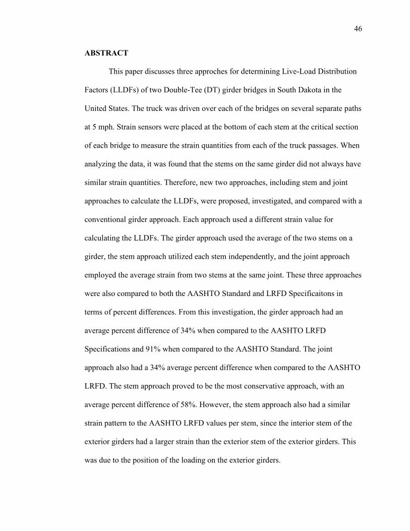
Bridge B

The second bridge tested has been in-service for 38 years. There are eight DT

girders connected by grout and a shear plate every 1.5 meters. Each girder is

approximately 1.2 meters in width, 584-mm deep, and contains seven prestressing

tendons per stem. The bridge is simply supported with a single span of 14.6 meters.

The girders bear on timber abutments. Pictures of the bridge can be seen in Figures 4a

and 4b. A visual inspection of the bridge was performed before the field tests, and a

map of the joint damage was created. Figure 5 shows the damage on the bridge.

Leakage through the joints, efflorescence, and corrosion of the shear plates were

observed in the joints between the DT girders. An example of the joint damage is

shown in Figure 6. Notice the efflorescence and leakage (staining) between the stems

of adjacent girders.

53

a) Road Surface b) Side View

Figure 4. Pictures of Bridge B (Credit: Brian Kidd)

Figure 5. Damage Map of Bridge B from Kidd et al. (2020)

54

Figure 6. Example of Staining on the Bridge B (Kidd et al. 2020)

FIELD TESTING (Kidd et al. 2020)

The two bridges, as described previously, were tested with a static load over

five separate paths on each bridge. The paths were selected such that each girder was

loaded at some point throughout the five paths. The five paths for the Bridge A and B

can be seen in Figure 7a and 7b, respectively. These figures also include the

dimensions of the DT girders for each bridge and the identification of the girders,

joints and stems. The data from Path A on Bridge A was lost while transferring data,

therefore, the maximum LLDFs are outliers in the figures and tables throughout this

paper (G1, S1 and S2, J1 for Bridge A).

55

a) DT Bridge A

b) DT Bridge B

Figure 7. Truck Paths for DT Bridges

To collect the strain values during the loading, surface-mounted strain gauges

were used. One strain gauge was placed on each stem (two per girder) of the girders.

The strain gauges were placed on the bottom of the stems at the mid-span of the

56

girder such that the maximum strain of the bridge was recorded. Each gauge had a

0.3-meter extension attached; thus, the strain value could be measured more

accurately. Fourteen strain gauges were used for Bridge A, and sixteen for Bridge B.

This placement was chosen to get the largest strain values possible during the field

test.

A truck matching the SD Legal Load Type 3 was driven across the bridges at

a speed of 8 km/hr, to represent a crawl speed loading. A picture of the test truck is

shown in Figure 9a. The total weight of the truck was 222.32 kN. The weight

distribution between axles is shown in Figure 9b. The axle with was approximately

2.2 meters. More information about field testing can be found in Kidd et al. (2020).

a) Side View

57

b) Axle Configuration

Figure 9. Truck used for Field Testing (Kidd et al. 2020)


The strain values from the field tests were recorded. Then, as mentioned

before, LLDFs were calculated by girder (traditional approach), by each stem, and by

each joint on the bridge. For all field strain-based calculations, Equation 1 was used.

�� ∑ �� (1)

Flexural strain is denoted by ε in Equation 1. Equation 2 is the suggested

AASHTO LRFD formula for LLDFs of DT girder bridges. In Equation 2, only the

spacing (S) changes among the three different approaches. The exterior girder LLDF

is calculated using the lever rule, per the AASHTO LRFD Specifications.

8� � 0.06 + � ��.� ��

��.� � ��.�

(2)

58

In the equation above, S is the spacing (ft), L is the span length (ft), tS is the

thickness of the slab (in), and Kg is the longitudinal stiffness (in3). The calculations

were completed in U.S. customary units because the data was collected as such (3.281

feet is equal to 1 meter). The AASHTO Standard Specifications is shown for the

LLDFs by girder. The AASHTO Standard Specifications (AASHTO 1996) provide

Equation 3 to determine LLDFs by girder. As indicated below, sequential equations

(Equations 4-6) in addition to Equation 3 are necessary to calculate the LLDFs. This

value is used for both interior and exterior girders.

8 � �9 (3)

� � �5.75 − 0.5"�# + 0.7"��1 − 0.2&#� (4)

& � ' �(� � (5)

' � )�1 + *# + ,⁄ .�./ (6)

S is the girder spacing (ft), µ is Poisson’s ratio, I is the moment of inertia (in4), J

is the torsional constant (in4), and NL is the number of lanes. The AASHTO LRFD

and AASHTO Standard equations are given in U.S. customary units, however, the

LLDFs are unitless. One meter is approximately 3.28 feet and 2.54 cm is equal to one

inch for reference. Figure 7 shows the labeling the girders (G), stems (S), and joints

(J) to reference during the discussion. All the numbering starts from the same side of

the bridge (i.e. joint J1 and stem S1 are on girder G1).The equations above were used

for all three of the approaches. The following subsections explain each of the three

approaches in more detail.

59

Girder Approach

This approach is the traditional way to determine LLDFs of a DT girder

bridge. To find the strain per girder, the average strain value of the two stems from a

single girder was calculated. While calculating the measured LLDFs, there were

instances where the strain values from the gauges on the same girder did not have

similar strain values. Since the stems of the same girder are nearly four feet apart

transversely, the load induced on each stem will be different. Thus, taking the average

of the two strains changed the strain value significantly. For Bridge A, the field

results for the girder approach and two AASHTO design values for are shown in

Figure 9a-b. The percent differences for both bridges can be seen in Table 1. It can be

seen that girder G1 has significantly larger percent differences (i.e. 144% and 160%).

Unfortunately, data from path A was lost after completing the field tests, therefore the

LLDF values are outliers in this study.

The comparison shows that the AASHTO LRFD-codified LLDFs are higher

than the field LLDF values in every case, except the exterior girder G7. Specifically,

the AASHTO LRFD values were, on average, 34.7% larger than the field LLDFs,

while the field LLDF for G7 was higher than the AASHTO LRFD value by 2.6%.

This phenomenon can be explained by the visual inspection showing that damage to

the longitudinal joint is present and causes a high LLDF for G7. Meanwhile, the

AASHTO Standard Specifications were significantly higher than any field LLDFs.

The AASHTO Standard was, at a minimum, 36% higher than the field LLDF and on

average, 90% larger. This is over conservative and unacceptable for design.

60

a) Bridge A (Path C)

b) Bridge A (Path E)

0.00

0.10

0.20

0.30

0.40

0.50

0.60

0.70

0.80

0.90

1 2 3 4 5 6 7

Gir

de

r LL

DF

Girder Number


0.00

0.10

0.20

0.30

0.40

0.50

0.60

0.70

0.80

0.90

1 2 3 4 5 6 7

Gir

de

r LL

DF

Girder Number


61

c) Bridge B (Path C)

d) Bridge B (Path E)

Figure 9a-d. LLDFs using the Girder Approach (Kidd et al. 2020).

For Bridge B, the comparison can be seen in Figure 9c-d. Girder G5 is the

only field LLDF that is greater than the AASHTO LRFD value. However, the field

LLDF is only 3% larger than the AASHTO LRFD. Again, the comparison of field

0.00

0.10

0.20

0.30

0.40

0.50

0.60

0.70

0.80

1 2 3 4 5 6 7 8

Gir

de

r LL

DF

Girder Number


0

0.1

0.2

0.3

0.4

0.5

0.6

0.7

0.8

1 2 3 4 5 6 7 8

Gir

de

r LLD

F

Girder Number


62

LLDFs and AASHTO codified LLDFs can be seen in Table 1. Leakage through the

joint between G4 and G5 is believed to be the cause of this high LLDF (Kidd et al.

2020). The minimum percent difference between the field LLDFs and the AASHTO

LRFD codified LLDFs is 29.8%. Again, the AASHTO Standard Specifications

significantly overestimate the field LLDFs by 91.5% on average. The AASHTO

Standard Specifications was included in this investigation since the DT bridges are

over thirty years old and were designed using the AASHTO Standard Specifications.

Table 1. Comparison of AASHTO LLDFs to Girder Approach

Bridge A Bridge B

LRFD Standard LRFD Standard

Girder Percent

Difference

Percent

Difference

Percent

Difference

Percent

Difference

G1 144.1* 160.4* 31.7 75.6

G2 34.1 95.9 14.8 83.5

G3 26.3 89.7 64.9 121.8

G4 38.9 99.7 49.3 110.5

G5 58.9 114.9 -2.9 68.4

G6 47.6 106.4 51.9 112.4

G7 -2.6 36.0 43.6 106.3

G8 - - 7.4 53.7

Average 34.7 90.4 33.3 91.5

*There is no data for Path A on Bridge A.

More discussion about the girder approach and AASHTO codified LLDF

values can be found in Kidd et al. (2020).

Stem Approach

With the strain values measured from the field test, Equation 1 was used to

calculate the LLDFs for all stems for each bridge. When calculating the AASHTO LRFD

63

and Standard values to compare with this approach, the average of the stem spacing was

used in the DT girder bridge equations from the AASHTO LRFD (Equation 2) and

Standard (Equation 3) respectively. It should be noted that the LLDFs of the stems on the

exterior girders were calculated using the lever rule for the AASHTO LRFD

Specifications. The reaction of the two stems was found using the lever rule, and a

multiple presence factor of 1.2 was applied to both stems.

Figure 10a-b compares the LLDFs by stem to the AASHTO design values for

Bridge A. Stem 13, which is the inside stem of the exterior girder, has a substantially

higher LLDF than the AASHTO LRFD-based LLDF value. Besides Stem 13, the rest of

the field LLDFs were lower than the AASHTO LRFD values. The percent differences for

the stem approach can be seen in Table 2. Specifically, Stem 13 has a value 7.5% higher

than the AASHTO Standard LLDF. It should be noted that Stem 13 on Bridge A is the

only time the field LLDF exceeded the codified LLDFs from the AASHTO Standard

Specifications.


0.00

0.05

0.10

0.15

0.20

0.25

0.30

0.35

0.40

0.45

1 2 3 4 5 6 7 8 9 10 11 12 13 14

Ste

m L

LDF

Stem Number


64



0

0.05

0.1

0.15

0.2

0.25

0.3

0.35

0.4

0.45

0.5

1 2 3 4 5 6 7 8 9 10 11 12 13 14

Ste

m L

LD

F

Stem Number


0.00

0.05

0.10

0.15

0.20

0.25

0.30

0.35

0.40

0.45

1 2 3 4 5 6 7 8 9 10 11 12 13 14 15 16

Ste

m L

LD

F

Stem Number


65


Figure 10a-d. LLDFs using the Stem Approach.

Figure 10c-d compares the field LLDFs from Bridge B to the two AASHTO

design codes. The percent differences for Bridge B can be seen in Table 2. Stem 10

has a field LLDF higher than the AASHTO LRFD value by 11.8%, showing similar

results to the girder approach. However, now there is another LLDF value greater

than AASHTO LRFD. Stem 4 is now 1.5% larger than the design value. In this case,

the AASHTO Standard is larger than all the field LLDFs. The difference in LLDFs

between adjacent stems, S4 and S5, may suggest joint damage on the joint between

G2 and G3.

0.00

0.05

0.10

0.15

0.20

0.25

0.30

0.35

0.40

0.45

1 2 3 4 5 6 7 8 9 10 11 12 13 14 15 16

Ste

m L

LD

F

Stem Number


66

Table 2. Comparison of AASHTO LLDFs to Stem Approach

Bridge A Bridge B


Stem Percent

Difference

Percent

Difference

Percent

Difference

Percent

Difference

S1 167.3* 178.2* 32.7 79.4

S2 138.7* 147.3* 81.2 76.9

S3 89.7 121.1 55.3 94.3

S4 41.3 80.8 -1.5 43.4

S5 57.6 94.9 83.5 117.4

S6 42.5 81.9 78.6 113.5

S7 54.7 92.4 64.4 101.9

S8 63.2 99.5 88.9 121.7

S9 37.4 77.4 90.2 122.6

S10 129.8 151.7 -11.8 33.5

S11 47.2 86.0 88.4 121.3

S12 99.0 128.5 70.0 106.5

S13 -25.0 -7.5 69.3 105.9

S14 89.8 121.0 65.6 102.9

S15 - - 21.7 16.6

S16 - - 74.8 114.1

Average 55.5 81.6 61.1 92.0

*Bridge A does not have data for S1 and S2.

The average of all the percent differences of the stem approach was

calculated. The AASHTO LRFD and AASHTO Standard have an average percent

difference from the field LLDFs of 55.5% and 81.6%, respectively. Stem 12 has a

noticeably smaller value than Stem 13, which are separated by only a joint. This is

another indicator of joint damage at that location. Path A data was lost when

transferring the data between data logger and computer, therefore the field LLDFs of

Stem 1 and 2 did not show a similar trend to the other exterior stems. As shown in

Figure 10b and 10d the lever rule accurately describes the strain in the exterior DT

67

girder. The inner stem of the exterior girder experiences more strain than the outer

stem, based on how the truck loads an exterior girder.

Joint Approach

Since the strain values in stems on the same girder were not similar, the stems

on either side of the same joint were investigated. The field LLDFs were calculating

by taking the average of two stems on a joint and the exterior stems were not

averaged with another value, similar to the stem approach. The AASHTO LRFD

equation used the spacing between the longitudinal joints, which is also the overall

width of the girder.

The comparison between the field LLDFs and the two AASHTO

specifications can be seen in Figures 11a-b. Table 3 shows the percent difference of

the LLDF values compared to the two AASHTO specifications for the bridges using

the joint approach. Joint 7 on Bridge A, including stems 12 and 13, is the only LLDF

higher than the AASHTO LRFD value by 22%. This is comparable to the result from

the stem approach, but the LLDF is higher in the joint approach. However, the girder

LLDF still yields the highest value.

68



0.00

0.10

0.20

0.30

0.40

0.50

0.60

0.70

0.80

0.90

1 2 3 4 5 6 7 8

Join

t LLD

F

Joint NumberField AASHTO LRFD AASHTO Standard

0.00

0.10

0.20

0.30

0.40

0.50

0.60

0.70

0.80

0.90

1 2 3 4 5 6 7

Gir

de

r LLD

F

Girder Number


69



0.00

0.10

0.20

0.30

0.40

0.50

0.60

0.70

0.80

0.90

1 2 3 4 5 6 7 8

Join

t LL

DF

Joint NumberField AASHTO LRFD AASHTO Standard

0.00

0.10

0.20

0.30

0.40

0.50

0.60

0.70

0.80

1 2 3 4 5 6 7 8 9

Join

t LLD

F

Joint Number


70


Figure 11a-d. LLDFs using the Joint Approach.

The joint approach data is different from the girder approach for Bridge B, as

seen in Figure 11c-d. Similar to the girder approach, the joint J6, between G5 and G6,

has a LLDF higher than the AASHTO LRFD value by 1%. However, joint J8 and J1

now have a value higher than AASHTO LRFD. The girder approach showed that the

exterior girder, G8 did not have a field LLDF higher than the AASHTO LRFD. Joint

8, which is the interior stem of G8, now exceeded the AASHTO LRFD value by

13.6% when using the joint approach. Joint J1 exceeded the AASHTO LRFD LLDF

by 21.6%. The AASHTO Standard value is higher than all the field, by an average of

95.2%. The AASHTO LRFD code is, on average, 28.9% higher than field LLDFs.

0.00

0.10

0.20

0.30

0.40

0.50

0.60

0.70

0.80

1 2 3 4 5 6 7 8 9

Join

t LL

DF

Joint Number


71

Table 3. Comparison of AASHTO LLDFs to Joint Approach

Bridge A Bridge B


Joint Percent

Difference

Percent

Difference

Percent

Difference

Percent

Difference

J1 141.0* 177.8* -21.6 89.0

J2 84.0* 132.6* 28.6 94.7

J3 21.9 86.1 20.4 88.1

J4 25.3 88.9 47.2 109.0

J5 20.4 84.8 64.9 121.8

J6 60.8 116.3 -1.0 70.0

J7 -22.0 47.1 44.1 106.7

J8 36.4 123.9 -13.6 58.7

J9 - - 18.8 118.5

Average 38.7 107.2 28.9 95.2

*There is insufficient data for J1 and J2.

The three different approaches of calculating distribution factors were

compared to the AASHTO LRFD and the AASHTO Standard using percent

differences. The percent differences for the girder, joint, and stem approaches are

shown in their respective tables (Tables 1-3). The average of the percent differences

was also calculated and used to compare the three different approaches. Table 4

compares the three approaches.

Table 4. Average Percent Differences of Three Approaches

Bridge A Bridge B

Percent

Difference

AASHTO

LRFD

AASHTO

Standard

AASHTO

LRFD

AASHTO

Standard

Girder 34.7 90.4 33.3 91.5

Joint 38.7 107.2 28.9 95.2

Stem 55.5 81.6 61.1 92.0

72

The average percent differences are shown for both the AASHTO LRFD and the

AASTHO Standard Specifications. The AASHTO Standard Specifications are very

inaccurate (i.e. 90% difference than field values), therefore there will be little discussion

about them. The AASHTO LRFD values are much closer to the field LLDFs. If the two

trials of each approacj (Bridge A and Bridge B) are averaged, the joint and girder

approaches are nearly identical at 33.8% and 34% respectively. The stem approach is

significantly higher, at 58.3%. However, the stem approach is more conservative than the

other two approaches, according to percent differences. The stem approach also has a

similar pattern to the field LLDFs, specifically when determining the stems on the

exterior girders. The LLDF of the stem on the inside of the exterior girder is larger than

the LLDF of the outer stem of the exterior girder. It is also larger than the LLDFs of the

stems on the interior girders. The joint approach also has higher LLDFs for the interior

joint of the exterior girder, than it does for the exterior joint of the exterior girder. The

difference between the stem and joint approach is that the interior LLDFs are higher than

the exterior LLDFs for the joint approach. In the stem approach, that is not the case.

Since Path A for the Bridge A did not have data, the field LLDF values are not

representative of the max LLDF. Thus, the corresponding percent difference values were

not included when calculating the average percent difference of each approach. The

asterisk in Tables 1, 2, and 3 note this. It is also worth noting the absolute value of the

percent difference values was used when calculating the average percent difference.

73

SUMMARY AND CONCLUSIONS

A comprehensive investigation on the determination of live-load distribution

factors (LLDFs) for two precast prestressed double-tee (DT) girder bridges in South

Dakota in the United States was conducted in three different ways. The LLDFs were

calculated based on the girder approach, stem approach, and joint approach. The

girder approach calculated the LLDFs using the average of the two stems from the

same girder, the stem approach used the strain values of each stem individually to

determine LLDFs, and the joint approach utilized the average strain of adjacent stems

at the same joint. The three approaches were compared to the AASHTO LRFD and

the AASHTO Standard Specifications in terms of the percent differences, so as to

judge the effectiveness of each approach. The following conclusions can be

determined based on the data analysis presented.

1. The girder approach was the most accurate approach to calculating the

AASHTO Specification-compliant LLDFs of the considered DT girder

bridges. The percent difference, when compared to AASHTO LRFD and

AASHTO Standard, was 34% and 91% respectively. The joint approach was

nearly as accurate as the girder approach. However, they may not always be

conservative when compared to the AASHTO LRFD specifications.

2. The stem approach was the most conservative of the three approaches relative

to the AASHTO LRFD and AASHTO Standard specifications, with average

percent differences of 58% and 87% respectively. This approach also showed

a similar pattern between the AASHTO LRFD LLDFs and the field LLDFs.

74

The interior stem of the exterior girder yielded higher LLDFs than the exterior

stem of the exterior girder, due to the position of the loading.

3. The AASHTO Standard Specifications were significantly higher than the field

values. The average percent differences are above 80% for every approach

used. However, there is one outlier. One AASHTO Standard LLDF value

compared to the stem approach was not conservative. It was proven that there

was significant joint damage near this stem, explaining the large field LLDF.

ACKNOWLEDGEMENTS


Department of Transportation (SDDOT) and the Mountain-Plains Consortium (MPC), a

University Transportation Center (UTC) funded by the U.S. Department of



authors, who are responsible for the facts and accuracy of the information presented. The

research team would like to thank everyone involved in the field testing that yielded the

data used in this study, especially, the SDDOT for the truck and other equipment used for

the field testing. The authors would like to thank Bob Longbons from the SDDOT and

Zach Gutzmer for their help with the field tests as well. The research team is grateful for

all those who participated in the field tests.

75

REFERENCES

AASHTO (American Association of State Highway and Transportation Officials).

(2012). LRFD Bridge Design Specifications. Washington, D.C.

AASHTO (American Association of State Highway Transportation Officials). (1996).

Standard Specifications for Highway Bridges, Sixteenth Edition Washington, D.C.

Cai, C. S., and Shahawy, M. (2004). “Predicted and Measured Performance of

Prestressed Concrete Bridges.” Journal of Bridge Engineering, 9(1), 4–13.

Culmo, M. P., and Seraderian, R. L. (2010). “Development of the northeast extreme tee

(NEXT) beam for accelerated bridge construction.” PCI J., 55(3), 86–101.

Fu, C. C., Elhelbawey, M., Sahin, M. A., and Schelling, D. R. (1996). “Lateral

Distribution Factor from Bridge Field Testing.” Journal of Structural Engineering,

122(9), 1106–1109.

Kidd, B., Rimal, S., Seo, J., Tazarv, M., and Wehbe, N., (2020). “Field Testing of

Deteriorating Double Tee Girder Bridges for Determination of Live Load

Distribution Factors and Dynamic Load Allowance.”

Kim, S., and Nowak, A. S. (1997). “Load distribution and impact factors for i-girder

bridges.” Journal of Bridge Engineering, 2(3).

Mensah, S. A., and Durham, S. A. (2014). “Live load distribution factors in two-girder

bridge systems using precast trapezoidal u-girders.” Journal of Bridge

Engineering, 19(2).

PCINE (Precast/Prestressed Concrete Institute Northeast). (2012). Guidelines for

Northeast Extreme Tee Beam (NEXT Beam), First Edition. PCINE, Belmont, MA.

76











concrete composite bridges under farm traffic.” Engineering Structures, 69.


next beam bridges." Master’s Thesis.

Torres, Victor J., (2012). "Live load testing and analysis of a 48-year-old double tee

girder bridge." Master’s Thesis.



12(6), 765–773.

Zokaie, T. (2000). “AASHTO-LRFD Live Load Distribution Specifications.” Journal of

Bridge Engineering, 5(2).

77

CHAPTER 3: EFFECT OF DAMAGE ON LIVE-LOAD DISTRIBUTION

FACTORS OF DOUBLE-TEE BRIDGE GIRDERS

Brian Kidd, EI, S.M. ASCE





Phone: (507) 456-3065

78

ABSTRACT

This paper aims to study the impact of damage on the live load distribution factors

(LLDFs) of two precast, prestressed double-tee (DT) girder bridges located on rural roads

where the bridge is deteriorating due to service loads. Field testing was completed on the

DT girder bridges to calculate the field LLDFs of each girder. The codified LLDFs were

calculated following the AASHTO LRFD and AASHTO Standard Specifications and

compared to the field values. The longitudinal joint damage was identified by visually

inspecting and measuring the different types and locations of damage by hand. Based on

the condition states from the AASHTO Manual for Bridge Element Inspection, the

identified damage on each joint was quantified in terms of a damage ratio considering the

severity of the damage. Then, the damage along the joints was split evenly among the

adjacent girders, to determine a girder damage ratio (GDR) defined as the amount of

longitudinal joint damage affecting the DT girder, used to determine the effect of the

damage on the LLDFs. Graphical comparison and linear regression methods were used to

identify a relationship between the LLDFs and GDR. Both methods suggested that when

the wheel loads were directly above the DT girders with high GDRs, the LLDFs were

higher. The regression yielded a correlation coefficient of 0.694 and 0.579 when the load

was over the two highest GDRs for each bridge, respectively. Both correlation coefficients

are significant when α = 0.05. From the analysis of the results, it can be concluded that the

longitudinal joint of the bridge was severely damaged such that the load could not be

appropriately distributed to adjacent DT girders as designed; thus, the LLDF increased.

79

INTRODUCTION

Precast, prestressed double-tee (DT) girders, also known as Northeast Extreme Tee

beams (NEXT beams), are easily constructed and have a fast time of construction (PCINE

2012). The DT girders can be efficiently placed on top of the abutments and the top flange

of the girders can be used as an integrated deck. Particularly, the DT girders are attached

to adjacent girders at the top flange, creating the deck surface. This is uncommon with most

typical girder bridges, as decking is poured on top to distribute vehicle loads to the girders.

With DT girder bridges, the load is distributed to the adjacent girders through the joint

connection at the top flanges. Hence, the live-load distribution factors (LLDFs) of DT

girder bridges should change with joint damage.

The AASHTO LRFD Design Specifications (AASHTO 2012) is the current code

used for designing bridges using LLDFs. The AASHTO Standard Specifications for

Highway Bridges (AASHTO 1996) was used until the latest edition, which was in 2002.

The AASHTO LRFD has developed LLDF equations for each type of bridge (AASHTO

2012). Huang and Davis (2017) found that the LRFD DT and I-girder sections should be

applicable for NEXT beams LLDF calculations, and the LRFD concrete channel section

may be overly conservative. It has been proven that the vehicle configuration

characteristics affected the LLDFs (Seo and Hu 2014; Seo et al. 2017). There has been

minimal research into LLDFs for DT girder bridges. Few researchers have conducted field

tests on DT girder bridges (Kidd et al. 2020; Singh 2012; Torres et al. 2019). Torres et al.

(2019) indicated that the AASHTO LRFD approach was conservative for a structurally

sound bridge. Kidd et al. (2020) found that the AASHTO LRFD approach was conservative

80

in nearly all instances, except for areas when damage was significant. Singh (2012) studied

different methods for calculating the AASHTO LRFD LLDFs for DT bridge design. It was

reported that the single-stem approach was more conservative for interior girders, and the

maximum of the two approaches were used for exterior girders.

The AASHTO Manual for Bridge Element Inspection (AASHTO 2013) is the basis

for categorizing individual bridge components based on its descriptive and quantitative

condition states descripting damage states. Specifically, the condition states are ranked

from one to four. One being good, or without damage, and four being severe, requiring a

structural review. With the condition states, damage quantification for in-service bridges

has recently been performed using image analysis techniques (Duque et al. 2018). Duque

et al. (2018) used pixel-based and photogrammetry-based analyses to determine crack

thickness and rust staining area. However, the issue of objectively categorizing bridge

components into four states is still prevalent. Using the AASHTO Manual still allows for

subjective results, since the classification of condition state is still dependent on the bridge

engineer and their experience. Meanwhile, Shinozuka et al. (2000) created a bridge damage

state and applied a bridge damage index, which quantified the damage state with a value.

Minor, moderate, major and collapsed are the four damage states with 0.1, 0.3, 0.75, and

1.0 as the respective corresponding bridge damage indexes from Shinozuka et al. (2000).

There have not been any studies on the in-depth investigation of a correlation

between damage state and LLDFs on DT girder bridges. Therefore, this paper is intended

81

to study the effect of longitudinal joint damage on the LLDFs of a DT girder bridge. The

focus of this study was on longitudinal joint damage to the DT girders and the effect it has

on the bridge using LLDFs. LLDFs were determined based on field tests and visual

inspections physically measured the amount and location of damage on the longitudinal

joints between girders. The quantified damage was then compared with the LLDFs to

determine if the longitudinal joint damage impacted the load distribution of the girders. A

direct comparison was done between the damage and field LLDFs, and a simple linear

regression was conducted to determine if a correlation was present.

BRIDGE DESCRIPTION

Bridge A

The first DT girder bridge selected for this study is 34 years old and is in-service

on a gravel road in Lincoln County, South Dakota. The bridge consists of seven

prestressed, DT girders bearing on concrete abutments. The girders are 762 mm deep,

with a 127 mm deep top flange, and have a span length of 11.6 meters. The longitudinal

joints have a welded steel plate connection spaced every 1.52 meters and then filled with

grout (Bohn 2017). Figure 1 shows a picture of the bridge. The cross section of one DT

girder is shown in Figure 2. Significant damage of the longitudinal joints between girders

was present and the damage is discussed later in this study.

82


Figure 1. Pictures of the DT Bridge Tested

Figure 2. Cross Section of Double-Tee Girder

Bridge B

The second DT girder bridge selected for this study is 38 years old and is in-

service on a gravel road in Moody County, South Dakota. The bridge has seven

prestressed, DT girders that bear on timber abutments. The girders are 584 mm deep,

with a 127 mm deep top flange, and a span length of 14.6 meters. The longitudinal joints

are a steel shear key with grout, similar to Bridge A. Figure 3 shows pictures of the

bridge and the cross section can be seen in Figure 4. Significant longitudinal joint

damage is present on this bridge and will be discussed in more detail later in this paper. It

is also important to note that G4 had a shear crack near the north abutment.

83

a) View of bridge from road surface b) View from bridge underneath

Figure 3. Description of 584-mm Deep DTG Bridge

Figure 4. Cross-Section of DT Girder on Bridge B

FIELD TESTING (KIDD ET AL. 2020)

Bridge A was tested on four different paths, such that each girder was loaded at

least once. The location of the wheels for Paths A-E are shown in Figure 5. A test was

conducted on girders G1 and G2, however, the data was lost. Bridge B was tested on five

different paths, which can be seen in Figure 6. A truck was loaded to a weight of 222 kN.

The truck was driven across the bridge at 8 km/hr, as a crawl speed live load. These tests

84

allowed the measurement of strain values for calculating field LLDFs. Strain gauges were

installed at the bottom of each stem, at the midspan of the bridge to record the largest

strain values possible.

Figure 5. Load Paths for Field Testing on Bridge A (Kidd et al. 2020)

Figure 6. Load Paths for Field Testing on Bridge B (Kidd et al. 2020)

85

The strain histories from Paths C and E of the field tests on both bridges are

shown in Figures 7a-d. Figure 7a shows the strain versus the location of the front axle of

the truck. It can be seen that the girder directly under the truck (G2, G3, and G4) had the

highest responses and consequently the highest field LLDFs. Figure 7b shows G7 having

a significantly higher strain value than the other girders, this is expected since G7 is an

exterior girder. This trend can be seen in all of the figures from the field testing. More

discussion on field testing can be found in Kidd et al. (2020).

a) Path C (Bridge A)

86

b) Path E (Bridge B)

c) Path C (Bridge B)

87

d) Path E (Bridge B)

Figure 7. Strain Response from Field Testing (Kidd et al. 2020)

From the strain graphs, field LLDFs were calculated for every girder over the five

paths. Table 1 and Table 2 shows the LLDFs from the field testing and the codified

LLDFs for both bridges. As seen in Table 1, there is only one field LLDF that exceeds

the AASHTO LRFD codified LLDF. G7 has a field LLDF 2.6% higher than the codified

LLDF. The same thing occurred in Table 2; G5 had an LLDF higher than AASHTO

LRFD codified LLDF. The purpose of this study is to explain that these outliers were

caused due to the longitudinal joint damage.

88

Table 1. Comparison of LLDFs for the DT Girder Bridge A

Table 2. Comparison of LLDFs for the DT Girder Bridge B

DAMAGE QUANTIFICATION

Damage quantification of bridge elements has yet to be standardized. Current

practices use qualitative terms, such as fair, poor, etc. (AASHTO 2013). This method is

subjective since it depends on the bridge inspector and their judgement. To quantify the

bridge damage, a new method was used to assign a numerical value to the qualitative

terms. A visual inspection was necessary to measure the amount and type of damage.

Then, to quantify the damage, the damage was given a weighted value based on the

G1 G2 G3 G4 G5 G6 G7

Path B 0.084 0.270 0.293 0.227 0.079 0.020 0.026

Path C 0.036 0.110 0.282 0.257 0.208 0.071 0.048

Path D 0.018 0.033 0.087 0.209 0.204 0.235 0.214

Path E 0.004 0.021 0.022 0.066 0.141 0.212 0.534

Max Field LLDF 0.084 0.270 0.293 0.257 0.208 0.235 0.534

AASHTO LRFD 0.52 0.381 0.381 0.381 0.381 0.381 0.52

AASHTO Standard 0.768 0.768 0.768 0.768 0.768 0.768 0.768

G1 G2 G3 G4 G5 G6 G7 G8

Path A 0.318 0.246 0.171 0.143 0.088 0.021 0.007 0.006

Path B 0.103 0.290 0.154 0.203 0.164 0.047 0.022 0.018

Path C 0.028 0.091 0.098 0.188 0.346 0.134 0.060 0.055

Path D 0.011 0.015 0.034 0.093 0.302 0.198 0.181 0.166

Path E 0.001 0.005 0.011 0.035 0.161 0.166 0.216 0.407

Max Field

LLDF 0.318 0.290 0.171 0.203 0.346 0.198 0.216 0.407

AASHTO

LRFD 0.438 0.330 0.330 0.330 0.330 0.330 0.330 0.438

AASHTO

Standard 0.705 0.705 0.705 0.705 0.705 0.705 0.705 0.705

89

severity and amount of the damage. The process used in Table 4 and 5 will be discussed

below in the following subsections.

Bridge Inspection

Before quantifying the damage, a visual inspection was performed on the bridge

specimen. The visual inspection was completed using tape measures, rulers, and a

camera. Both the length and the thickness of the visible damage was measured. A visual

inspection revealed damage at the longitudinal joints between the girders, but no

significant damage on the girders themselves. Figures 8 and 9 show examples of the

longitudinal joint damage. Figure 8 shows an example of leakage through the joint,

allowing water to seep through. Figure 9 shows an example of staining and corrosion in a

joint. Figures 10 and 11 show the location and type of the damage on both bridges

respectively. The damage was identified, and the affected area was measured by tape

measure and ruler. The damage was identified using the AASHTO Manual for Bridge

Element Inspection (AASHTO 2013) condition states (CS).

Figure 8. Leakage in the Joint Allowing Water in Between Girders (Credit: Brian Kidd)

Leakage

90

Figure 9. Staining and Corrosion of the Longitudinal Joint (Credit: Brian Kidd)

Figures 10 and 11 show the location and type of the damage on bridges A and B

respectively. The damage was identified, and the affected portion was measured by tape

measure and ruler. The damage on Bridge A was measured using areas since the bridge

clearance and water height allowed the research team to get close enough to the joints

underneath the bridge. Bridge B had a deeper water level and a larger clearance, therefore

only the length was able to be measured. The damage was identified using the AASHTO

Manual for Bridge Element Inspection (AASHTO 2013) condition states (CS).

Staining Corrosion

91

Figure 10. Damage Map of DT Girder Bridge A

92

Figure 11. Damage Map of DT Girder Bridge

93

Damage Type and Portion

The second columns of Table 4 and 5 describes the damage type. Damage along

the longitudinal joints included leakage, staining, and corrosion of the steel plates. When

the grout in the joint deteriorates, water can get in the joint and leak through. As it

deteriorates more, efflorescence or staining occurs on the concrete below the joint. The

joint includes a steel plate every 1.52 meters along the girder. As the water penetrates the

joint, it can accelerate the corrosion of the steel plates. For example, damage [J3:1] has

both staining (S) and corrosion (C) present. The third columns of Table 4 and 5 shows the

amount of damage, in terms of area. The portion was measured by hand using a tape

measure. It should be noted that, Bridge B only used the length of the damage and Bridge

A used the area of the damage present. The large clearance and water level underneath

the bridge did not allow the research team to get close enough to measure the width of the

damage. Instance [J3:1] had 2932.3 cm2 of staining and 153.2 cm2 of corrosion at the

joint.

AASHTO BDI and Damage State

According to the AASHTO Bridge Element Inspection Manual (AASHTO 2013), the

elements are inspected and classified as one of four CS. CS-1 shows no damage, CS-2 is

described as fair, CS-3 is a poor element state, and CS-4 is classified as severe damage.

The AASHTO BDI for each damage instance is shown in fourth column of the table.

Once the visual inspection was completed and the AASHTO CS were applied, the next

step is to quantify the damage in terms of damage ratio (Shinozuka et al. 2000). Using the

technique developed by Shinozuka et al. (2000), a damage state was applied to each

94

damage type. CS-2 was given a damage state of 0.3 and CS-3 was given a value of 0.75.

CS-1 and CS-4 are also given damage states, however, CS-1 is considered no damage and

there was no severe damage, CS-4, found. Table 3 shows the CS and corresponding

damage states. For example, damage [J3:1] was classified as poor (CS-3) for both

staining and corrosion and given a damage state of 0.75.

Table 3. Damage States Used for Damage Quantification (Adopted from Shinozuka et

al. 2000)

Condition

State

Damage

Type

Damage

State

CS-1 None 0

CS-2 Fair 0.3

CS-3 Poor 0.75

CS-4 Severe 1

Weighted Damage Portion and Damage Ratios

The damage portion (cm2 or cm), determined by measuring the visual damage,

was multiplied by the damage state (i.e. 0.3 or 0.75) to quantify the severity of the

damage. This can be seen in column six of Table 4 and 5. From the weighted damage

area (the damage area multiplied by the damage state), a damage ratio was calculated by

dividing the damage at each instance by the sum of the weighted damage areas for the

entire bridge. For example, [J3:1] multiplied the damage amount by 0.75 for a weighted

damage portion of 2314.2 cm2. Then, 2314.2 cm2 was divided by 14196.9 for a damage

ratio of 0.163.

95

The damage ratios along the same longitudinal joint were summed together to

calculate the joint damage ratio (JDR) in column eight. To compare the damage ratio to

the damage on the longitudinal joints, the JDR was converted to a girder damage ratio

(GDR). The GDR represents the amount of longitudinal joint damage affecting the DT

girder. The GDR was calculated by dividing the JDR by two and distributed equally to

the adjacent girders. For example, the JDR on Joint J3 was split between girders G3 and

G4. The GDRs for both bridges are shown in Table 6.

96

Table 4. Damage Type, Portion, and Quantification from Bridge A

Location Damage Type Damage Portion (cm2) AASHTO BDI Damage State Weighted

Damage

Portion

(cm2)

Damage

Ratio

Joint

Damage

Ratio L S C L S C

(AASHTO

2013)

(Shinozuka et al.

2000)

[J1:1] X O X - 593.5 - Poor 0.75 445.2 0.031 0.031

[J2:1] X O O - 2685.5 166.1 Poor 0.75 2138.7 0.151 0.159

[J2:2] X O O - 103.2 62.9 Poor 0.75 124.6 0.009

[J3:1] X O O - 2932.3 153.2 Poor 0.75 2314.1 0.163 0.186

[J3:2] O X X 129 - - Fair 0.3 38.7 0.003

[J3:3] X O X - 387.1 - Poor 0.75 290.3 0.020

[J4:1] X O X - 116.1 - Poor 0.75 87.1 0.006

0.093

[J4:2] O X X 645.16 - - Fair 0.3 193.5 0.014

[J4:3] X O X - 467.7 - Poor 0.75 350.8 0.025

[J4:4] O X X 67.7 - - Fair 0.3 20.3 0.001

[J4:5] X O X - 154.8 - Poor 0.75 116.1 0.008

[J4:6] O X X 77.4 - - Fair 0.3 23.2 0.002

[J4:7] X O O - 580.6 121 Poor 0.75 526.2 0.037

[J5:1] X O O - 1625.8 61.3 Poor 0.75 1265.4 0.089 0.304

[J5:2] X O O - 3987.1 90.3 Poor 0.75 3058.1 0.215

[J6:1] X O X - 2754.8 - Poor 0.75 2066.1 0.146

0.226 [J6:2] X O O - 822.6 112.9 Poor 0.75 701.6 0.049

[J6:3] O X X 1445.2 - - Fair 0.3 433.5 0.031

*Damage that is present is marked with an “O” and damage not present is marked with an “X”. “L” is leakage, “S” is staining, and “C” is

corrosion.

97

Table 5. Damage Type, Portion, and Quantification from DT Girder Bridge B

Location

Damage Type Damage Portion (cm) AASHTO BDI Damage State Weighted Damage

Portion (cm)

Damage

Ratio

Joint

Damage

Ratio L S C L S C (AASHTO 2011) (Shinozuka et

al. 2001)

[J1:1] X O X - 143.3 - Poor 0.75 107.475 0.044

0.117 [J1:2] O X X 75 - - Fair 0.3 22.5 0.009

[J1:3] X O X - 207.3 - Poor 0.75 155.48 0.064

[J2:1] X O X - 679.7 - Poor 0.75 509.775 0.209

0.229 [J2:2] X O X - 30 - Poor 0.75 22.5 0.009

[J2:3] X O X - 35 - Poor 0.75 26.25 0.011

[J3:1] X O X - 33.3 - Poor 0.3 9.99 0.004

0.148 [J3:2] O X X 35 - - Fair 0.3 10.50 0.004

[J3:3] X O X - 429.8 - Poor 0.75 322.35 0.132

[J3:4] X X O - - 22.9 Poor 0.75 17.175 0.007

[J4:1] X O X - 86.72 - Poor 0.75 65.04 0.027

0.093 [J4:2] O X X 42.9 - - Fair 0.3 12.87 0.005

[J4:3] X O X - 179.8 - Poor 0.75 134.85 0.055

[J4:4] X X O - - 17.8 Poor 0.75 13.35 0.005

[J5:1] X O X - 186.2 - Poor 0.75 139.65 0.057 0.199

[J5:2] X O X - 460.2 - Poor 0.75 345.15 0.142

[J6:1] X O X - 120.1 - Poor 0.75 90.075 0.037 0.098

[J6:2] X O X - 199.5 - Poor 0.75 149.625 0.061

[J7:1] X O X - 40 - Poor 0.75 30 0.012

0.116

[J7:2] X O X - 140.2 - Poor 0.75 105.15 0.043

[J7:3] O X X 30 - - Fair 0.3 9 0.004

[J7:4] X O X - 35 - Poor 0.75 26.25 0.011

[J7:5] X O X - 149.4 - Poor 0.75 112.05 0.046

*Damage that is present is marked with an “O” and damage not present is marked with an “X”. “L” is leakage, “S” is staining, and “C” is

corrosion.

98

Table 6. Girder Damage Ratios

Girder Bridge A Bridge B

G1 0.016 0.059

G2 0.095 0.173

G3 0.173 0.188

G4 0.140 0.120

G5 0.199 0.146

G6 0.265 0.149

G7 0.113 0.107

G8 - 0.058

LLDF Determination

The LLDFs were calculated using the field data and the AASHTO LRFD and

Standard Specifications. To determine the LLDFs using field values, the average strain, γ,

of the stems on a single girder was divided by the sum of the average strain per girder.

Equation 1 was used when determining field LLDFs.

�� :�∑ :� (1)

The DT girder bridge section from the AASHTO LRFD (AASHTO 2012) was

used for calculating codified LLDFs. Equation 2 is given for two lanes loaded, interior

LLDFs for a DT section. For exterior girders, the lever rule was used to determine the

LLDF for the exterior girders. A unit wheel load was placed with the exterior tire 0.61

meters from the edge of the curb. The reaction of the outer stem of the exterior girder was

determined using the lever rule and then doubled to account for the second stem on the

girder. This value was multiplied by 1.2, the multiple presence factor for two lanes

loaded.

99

8� � 0.075 + � �;./��.< ��

��.� � ��.�

(2)

The AASHTO LRFD designates S as the center-to-center spacing, L as the span

length, Kg is the longitudinal stiffness, and ts is the deck thickness.

The AASHTO Standard Specifications (AASHTO 2002) has its own equation for

LLDFs in Section 3.23.4.3. Unlike the AASHTO LRFD, the AASHTO Standard

Specifications uses the equations below for both interior and exterior DT girders.

8 � �/� (3)

� � �5.75 − 0.5"�# + 0.7"��1 − 0.2&#� (4)

& � ' �(� � when W/L < 1 (5)

' � >��5?#@A B�/�

(6)

In the equations above, S is the center-to-center girder spacing (ft), NL is the

number of traffic lanes, W is the width of the bridge (ft), L is the span length (ft), I is the

moment of inertia of a girder (in4), J is the Saint-Venant torsional constant (in4), and µ is

the Poisson’s ratio for the girders. The equations above are in U.S. customary units.

These equations were used because the data was collected in U.S. customary units. For

reference, 3.281 feet is approximately 1 meter and 1 inch is approximately 25.4

millimeters. The LLDFs calculated using the field strain values, AASHTO LRFD and

AASHTO Standard Specifications are shown in Table 1 and 2.

100


Comparison with Field LLDFs

To investigate the effect of longitudinal joint damage on the LLDFs, a direct

comparison and a simple statistical analysis were conducted. The direct comparison

included a double bar chart comparing the GDR to the LLDF for the four paths. These

can be seen in Figures 12 and 13. Figure 12a shows the comparison for Path B, when G2

and G4 were loaded. Here we see when a high GDR does not always correlate with a

high LLDF value. G6 has the highest GDR, yet one of the lowest LLDF values. Figure

12b shows the results when girders G3 and G5 are loaded.

a) Path B b) Path C

101

c) Path D d) Path E

Figure 12a-d. Direct Comparison of LLDFs to JDR for Load Paths on Bridge A

Again, sometimes high LLDFs correlate with high GDRs and some do not. This

can be seen in both bridges. However, looking at the figures from the direct comparison,

it is clear that there are instances where both the LLDF and GDR are high. For example,

in Figure 12c and 13b, the largest GDR value has the highest LLDF as well. There are

multiple instances where the higher GDR values coincide with relatively large LLDF

values as well. In Figure 12d and 13c there is a weak correlation with high GDR and high

LLDF. From looking at the load paths and the direct comparison graphs, it was clear that

the location of the load was crucial. When the wheels of the truck were located over the

girders with a high damage ratio, then the GDR caused an increase in LLDFs.

102

a) Path A b) Path B

c) Path C d) Path D

e) Path E

Figure 13. Direct Comparison of LLDFs to JDR for Load Paths on Bridge B

103

To quantify this relationship, a simple linear regression was performed on the

field data to evaluate the correlation of the GDR on the LLDF. The simple linear

regression was done on the data from each path respectively. The linear regressions of

each path tested are shown in Figures 14 and 15. The coefficient of determination, R2,

was calculated first. To convert R2 to r, simply take the square-root of R2. The

corresponding coefficient of correlations were calculated and shown in Tables 9 and 10.

a) Path B b) Path C

c) Path D d) Path E

Figure 14. Simple Linear Regression of Load Paths for Bridge A

104

a) Path A b) Path B

c) Path C d) Path D

e) Path E

Figure 15. Simple Linear Regression of Load Paths for Bridge B

105

The coefficient of determination, R2, was calculated first. To convert R2 to r,

simply take the square-root of R2. The corresponding coefficient of correlations were

calculated and shown in Tables 7 and 8. From the correlation coefficient values

calculated for Bridge A, the GDRs in Path D have a significant correlation to the LLDFs.

Path D has the wheel load directly above the girders with the highest damage. The

coefficient of correlation, r, for Path D is 0.694. Typically, a coefficient of correlation

great than 0.7 represents a strong correlation (Schober et al. 2018). Statistically, an r =

0.694 with n = 14 is significant when α = 0.01. It can also be seen that the correlation

coefficients increase from Path A to Path D, where the load is closer to the larger GDRs.

Path C and Path E both have a weak correlation, but Path A has no correlation. As seen in

Table 7, the correlation coefficient increases as the load gets closer to the damaged joints

(i.e. Path D). This statistical analysis compliments the direct comparison, indicating that

damage on the longitudinal joints below the load will increase the LLDF.

From the simple statistical analysis of Bridge B, a trend similar to Bridge A can

be seen. The correlation coefficient is largest, r = 0.579, when the load is directly above

the girders with the largest GDR value. This is still a moderate correlation and significant

when α = 0.05. The correlation coefficient values decrease as the load moves away from

girders G2 and G3 (girders with the highest GDRs). The remaining paths show weak or

no correlation between the LLDFs and GDRs. Comparing the two bridges, the damage is

more evenly distributed on Bridge B than Bridge A.

106

Table 7. R2 and Correlation Coefficients from the Linear Regression for Bridge A

R2 r

Path B -0.0286 -0.169

Path C 0.1169 0.342

Path D 0.4822 0.694

Path E 0.0339 0.184

Table 8. R2 and Correlation Coefficients from the Linear Regression for Bridge B

R2 r

Path A 0.0048 0.0693

Path B 0.3349 0.5787

Path C 0.1496 0.3868

Path D 0.0023 0.0480

Path E 0.2283 -0.4778

Comparison with AASHTO LLDFs

Another indicator that the damage was affecting the loading of the bridge girders

is the comparison of the field LLDFs to the AASHTO codified LLDFs. The current

AASHTO LRFD Specifications are used to calculate design LLDFs for the bridge

girders. Codified LLDFs are determined according to Equation 2. The field LLDFs for

both bridges are compared to the respective codified LLDFs in Figure 16. The little

research done suggests that the AASHTO LRFD LLDFs are conservative for DT/NEXT

beams (Kidd et al. 2020; Torres et al. 2019).

107

a) Path C (Bridge A)

b) Path E (Bridge A)

0.00

0.10

0.20

0.30

0.40

0.50

0.60

0.70

0.80

0.90

1 2 3 4 5 6 7

Gir

de

r LLD

F

Girder Number


0.00

0.10

0.20

0.30

0.40

0.50

0.60

0.70

0.80

0.90

1 2 3 4 5 6 7

Gir

de

r LLD

F

Girder Number


108

c) Path C (Bridge B)

d) Path E (Bridge B)

Figure 16. Comparison of Field LLDFs with Codified LLDFs (Kidd et al. 2020)

Looking at Table 1, the only field LLDF that exceeds the AASHTO LRFD

LLDFs on Bridge A is G7 from Path E. The LLDFs and corresponding percent

differences can be seen in Table 9. The exterior girder had a field LLDF of 0.534 and the

AASHTO LRFD design LLDF was only 0.52. Again, Path E loads the joints with some

0.00

0.10

0.20

0.30

0.40

0.50

0.60

0.70

0.80

1 2 3 4 5 6 7 8

Gir

de

r LL

DF

Girder Number


0

0.1

0.2

0.3

0.4

0.5

0.6

0.7

0.8

1 2 3 4 5 6 7 8

Gir

de

r LLD

F

Girder Number


109

of the largest JDRs. The remainder of the paths did not have field LLDFs that exceeded

the design LLDFs. However, G3 has the highest interior LLDF and one of the largest

GDR values, at 0.173. This also suggests an increase of LLDFs due to longitudinal joint

damage. The GDRs are found in Table 6.

Table 9. Percent Differences of Field and Codified LLDFs for DT Girder Bridge A

Girder ID Field Max

AASHTO LRFD AASHTO Standard

LLDF Percent

Difference LLDF

Percent

Difference

G1 0.084 0.520 -144.4 0.768 -160.6

G2 0.270 0.381 -34.1 0.768 -96.0

G3 0.293 0.381 -26.1 0.768 -89.5

G4 0.257 0.381 -38.9 0.768 -99.7

G5 0.208 0.381 -58.7 0.768 -114.8

G6 0.235 0.381 -47.4 0.768 -106.3

G7 0.534 0.520 2.66 0.768 -35.9


For Bridge B, Table 2 compares the field LLDFs to the codified LLDFs. The

corresponding percent differences are shown in Table 10. Girder G5 is the only instance

where the field LLDF exceeds the AASHTO LRFD value, by 4.7%. However, this girder

was not loaded on the path that also had a high correlation coefficient (Path B). This does

not follow the same trend as Bridge A, however, this is due to a shear crack in girder G4.

The shear crack was not included in the damage ratios because the damage ratios only

include the damage to the longitudinal joints between girders, therefore the relationship

cannot be seen in this analysis. The second largest field LLDF is on girder G2. Since Path

110

B loaded girder G2 and had the highest correlation coefficient, it suggests that

longitudinal joint damage was the reason for the higher field LLDF even though it did not

exceed the AASHTO LRFD value.

Table 10. Percent Differences of Field and Codified LLDFs for DT Girder Bridge B

Girder ID Field Max

AASHTO LRFD AASHTO Standard

LLDF Percent

Difference LLDF

Percent

Difference

G1 0.318 0.438 -31.8 0.705 -75.7

G2 0.290 0.330 -12.9 0.705 -83.4

G3 0.171 0.330 -63.5 0.705 -121.9

G4 0.203 0.330 -47.7 0.705 -110.6

G5 0.346 0.330 4.7 0.705 -68.3

G6 0.198 0.330 -50.0 0.705 -112.3

G7 0.216 0.330 -41.8 0.705 -106.2

G8 0.407 0.438 -7.3 0.705 -53.6

CONCLUSIONS

This paper aims to study the effect of longitudinal joint damage on the live-load

distribution factors (LLDFs) of double-tee (DT) girder bridges. Using field results from the

live loads, the LLDFs were calculated for each girder. A visual damage inspection and the

AASHTO Bridge Element Inspection Manual were used to identify the damage on the

longitudinal joints. Then, the damage was quantified with a weighted damage approach

and a girder damage ratio (GDR) was determined. The LLDFs were compared to the

111

damage ratios using a direct comparison and a simple linear regression. From the results,

the following conclusions can be determined:

1. Longitudinal joint damage, mostly condition state 3 (CS-3), can cause LLDFs

of a DT girder bridge to exceed the AASHTO LRFD design values. In this

case, an exterior girder has a larger field LLDF than the design value by 2.6%.

This is significant since previous research suggested AASHTO LRFD design

LLDFs are conservative for DT bridges.

2. The AASHTO Standard Specifications are still over conservative for LLDFs

of DT girder bridges, even when longitudinal joints have damage classified as

CS-3. This Specification is outdated and overly conservative.

3. Damage along the longitudinal joints correlates to larger LLDFs when the

damaged joints are directly under the load path. A direct comparison shows

significantly larger LLDFs on the girders with the two largest GDRs. A

correlation coefficient of 0.694 was found for Path D on Bridge A, and a

correlation coefficient of 0.579 was found for Path B on Bridge B. Both

values are significant when α = 0.05. This linear regression shows a high

correlation for Bridge A and a moderately strong correlation for Bridge B.

ACKNOWLEDGEMENTS

The work presented in this paper conducted with financial support from the

South Dakota State University (SDSU) and Mountain-Plains Consortium (MPC), a


Transportation (USDOT). The contents of this paper reflect the views of the authors, who

112

are responsible for the facts and accuracy of the information presented. The research team

would like to thank everyone involved in the field testing that yielded the data used in

this study, especially, the South Dakota Department of Transportation (SDDOT) for the

truck and other equipment used for the field testing. The authors would like to thank Bob

Longbons from the SDDOT and Zach Gutzmer for their help with the field tests as well.

The research team is grateful for all those who participated in the field tests.

113

REFERENCES


(2012). LRFD Bridge Design Specifications, Washington, D.C.


(2013). Manual for Bridge Element Inspection, Washington, D.C.

AASHTO (American Association of State Highway Transportation Officials). (1996).

Standard Specifications for Highway Bridges, Sixteenth Edition Washington, D.C.

Bohn, Lucas Michael (2017) "Rehabilitation of longitudinal joints in double-tee girder

bridges" Theses and Dissertations. South Dakota State University, Brookings, SD.

Duque, L., Seo, J., and Wacker, J. (2018). “Bridge deterioration quantification protocol

using UAV.” Journal of Bridge Engineering, 23(10), 04018080.

Huang, J., and Davis, J. (2018). “Live load distribution factors for moment in NEXT

beam bridges.” Journal of Bridge Engineering, 23(3), 06017010.

Kidd, B., Rimal, S., Seo, J., Tazarv, M., and Wehbe, N., (2020). “Field Testing of

Deteriorating Double Tee Girder Bridges for Determination of Live Load

Distribution Factors and Dynamic Load Allowance.”

PCINE. (2012). “Guidelines for northeast extreme tee beam (NEXT Beam), First

Edition,” Precast Concrete Institute Northeast (PCINE), Belmont, MA.

Schober, P., Boer, C., and Schwarte, L. A. (2018). “Correlation Coefficients.” Anesthesia

& Analgesia, 126(5), 1763–1768.




114



Shinozuka, M., Feng, M. Q., Lee, J., and Naganuma, T. (2000). “Statistical analysis of

fragility curves.” Journal of Engineering Mechanics, 126(12), 1224–1231.


next beam bridges" Masters Theses 1911 - February 2014. 816.

Torres, V., Zolghadri, N., Maguire, M., Barr, P., and Halling, M. (2019). “Experimental

and analytical investigation of live-load distribution factors for double tee

bridges.” Journal of Performance of Constructed Facilities, 33(1), 04018107.

Zokaie, T. (2000). “AASHTO-LRFD live load distribution specifications.” Journal of

Bridge Engineering, 5(2), 131–138.

CHAPTER 4: PARAMETRIC STUDY OF PRECAST DOUBLE-TEE

BRIDGES USING LIVE-LOAD DISTRIBUTION FACTORS

Brian Kidd, EI, S.M. ASCE

115





Phone: (507) 456-3065

116

ABSTRACT

This paper aims to study the effects of different parameters of a double-tee girder

bridge on the live-load distribution factors (LLDFs). Field testing was conducted of two

double-tee girder bridges. From the field tests, LLDFs were calculated. A computer

model was made for each double-tee girder bridge using solid and shell elements in

SAP2000. The models were calibrated with the field LLDFs and then different

parameters were adjusted individually to see the variation in LLDFs. Span length,

concrete strength, deck width, diaphragm usage, and width to length ratio were

investigated in this parametric study for double-tee girder bridges. The AASHTO LRFD

interior LLDFs were generally accurate for the DT girder bridges with significant joint

damage. However, when Bridge B had a span length less than 12.2 meters, the AASHTO

LRFD LLDFs were exceeded by the analytical LLDFs. This was due to a shear crack in

one of the girders. Deck width, concrete strength, and diaphragm location had very little

influence on the LLDFs. The width-length ratio may be used as an indication to bridge

rating engineers that LLDFs may be conservative when damage is present on DT bridges.

The LLDFs decreased as the span length increased, which is in agreement with current

literature and the AASHTO LRFD code. The exterior LLDFs also decreased as span

length increased, which is not in agreement with the AASHTO exterior LLDFs calculated

using the lever rule. The results are discussed herein.

117

INTRODUCTION

Live-load distribution factors (LLDFs) are an important parameter used for both

design and rating of a bridge. LLDFs describe how the bridge is able to distribute the

load transversely, from the girders directly under the load to the remaining girders. The

AASHTO LRFD Specifications (AASHTO 2012) are the current design standard for

LLDFs of girder bridges. Before AASHTO LRFD, the AASHTO Standard Specifications

(AASHTO 1996) was used for the codified LLDFs when designing bridge girders.

Zokaie (2000) studied the AASHTO Standard LLDF equations and found that they were

only accurate for common bridges (e.g. a girder spacing of 1.8 m and a span length of 18

m).

There are many studies out there that investigate LLDFs, but there is little

research done on the LLDFs of DT girder bridges. Double-tee (DT) girder bridges are

commonly used on county roads in South Dakota. DT girders, also known as northeast

extreme tee (NEXT) beams, are desirable for their ease and simplicity of construction

(Culmo and Seraderian 2010). DT girders are placed side-by-side on abutments and

connected at the flange with a connection consisting of grout and steel plates placed

every 1.2 meters. Previous studies (Wehbe et al., 2016; Tazarv et al., 2019) have

demonstrated that this joint detailing is not sufficient for service and strength limit states

and proposed new detailing or rehabilitation techniques to improve the DTG longitudinal

joint performance. Damage along the longitudinal joints between DT girders is

significant since this type of damage impacts the transverse load distribution.

118

There are only a few studies on field testing of DT girder bridges. Torres (2016)

field tested a DT girder bridge with significantly deteriorated flanges. Torres found that

the AASHTO LRFD flexural LLDFs provided LLDF values consistent with that of a DT

girder bridge with significantly deteriorated flanges, implying that it may be conservative

for a DT bridge with little to no damage. Kidd et al. (2020) field tested two damaged DT

girder bridges and concluded that the AASHTO Standard LLDFs were overly

conservative in every instance, whereas the AASHTO LRFD LLDFs were, in most cases,

conservative for DT girder bridges.

There have also been some analytical studies of DT girder bridges in the past few

years. Finite element models (FEMs) have been developed for DT girder bridges (Singh,

2012; Torres, 2016). Torres (2016) was able to accurately model a DT girder bridge in

SAP2000/CSi Bridge using shell elements and link elements. Torres used link elements

to represent the loss in shear stiffness as a result of the deteriorated flanges. Singh (2012)

found that flexural LLDFs decrease as the DT girder span length increases, which is in

agreement with the AASHTO LRFD equations for LLDFs and other researchers. Huang

and Davis (2017) created an FEM in ABAQUS and a simplified model in CSi Bridge and

found good agreement between the two models.

The use of analytical models to further investigate the accuracy of the AASHTO

LRFD LLDFs is crucial. Many studies have used analytical models to investigate LLDFs

(Seo and Hu, 2014; Seo and Hu, 2015; Seo et al., 2014a,b; Seo et al., 2017). Yousif and

119

Hindi (2007) compared the AASHTO LRFD LLDFs with an FEM of prestressed I-girder

bridges and found that the codified LLDFs were inconsistent when different parameters

like girder spacing, span length, etc. were varied. It is inefficient and expensive to field

test many different DT bridges, therefore, FEMs should be used to investigate the effect

of different parameters on the LLDFs of DT girder bridges.

The purpose of this study was to create an accurate model of two DT girder

bridges with significantly damaged longitudinal joints. To accomplish this goal, strain

data from field tests were used to calibrate two models developed on CSi Bridge. Once

the models were calibrated, a parametric study was conducted to identify the affect that

parameters, such as span length and deck width, have on the LLDFs. Then, they can be

compared to the AASHTO LRFD LLDFs to identify the accuracy of the codified LLDF

equations. The bridge descriptions, field testing results, model calibration, and the results

of the parametric study are discussed in the following sections.

BRIDGES TESTED

Bridge A

The first DT girder bridge tested was 34 years old and had seven prestressed, DT

girders. The girders are 762 mm deep and the span length is 11.6 meters. The DT girders

are supported by concrete abutments with no skew angle. The wearing surface of the

bridge is gravel. The girders are connected using a steel plate and grout connection. The

120

steel plates are placed every 1.2 meters along the longitudinal joints. Pictures of the

bridge are shown in Figures 1a and 1b.

a) Surface b) Side View

Figure 1. Pictures of Bridge A

Since the bridge is in-service, there is significant damage along the longitudinal

joints. The locations and types of damage can be seen in Figure 2. Figure 3 shows some

of the damage present on this DT girder bridge. The cross section and the location of the

strain gauges used for field tests can be seen in Figure 4.

121

Figure 2. Damage Map of Bridge A from Kidd et al. (2020)

Figure 3. Efflorescence and Corrosion between G7 and G6 on Bridge A

Efflorescence Corrosion

122

Figure 4. Cross Section of DT Girder from Bridge A

Bridge B

The second DT girder bridge tested was 38 years old and had eight prestressed,

DT girders. The girders are 584 mm deep and the span length is 14.6 meters. The DT

girders are supported by timber abutments with no skew angle. The wearing surface is

gravel. The girders are connected using a steel plate and grout connection. The steel

plates are spaced at 1.2 meters along the longitudinal joints. The bridge can be seen in

Figures 5a and 5b.


Figure 5. Pictures of Bridge B

123

The bridge has significant damage on the longitudinal joints. The damage can be

seen in Figure 6. It is also noteworthy that a shear crack was present on the north end of

the girder G4. An example of the staining on Bridge B is shown in Figure 7. Figure 8 is a

typical cross-section for a 584 mm deep DT girder in South Dakota. The strain gauges

used for field testing can also be seen.

Figure 6. Damage Map of Bridge B from Kidd et al. (2020)

124

Figure 7. Example of Staining on Bridge B

Figure 8. Cross Section of DT Girder from Bridge B

REVIEW OF FIELD TESTS

Field Test Summary

The DT bridge was tested using a crawl speed load to determine the strain of the

girders. The goal of the tests was to determine the flexural LLDFs of the DT girders. A

truck that weighed 222 kN was used for the field tests. The truck is shown in Figure 9

and the axle configuration of the test truck can be seen in Figure 10.

125

Figure 9. Truck Used for Field Testing of Bridges A and B

Figure 10. Axle Configuration of the Truck used in Field Tests

The truck was applied at 8 km/h across five different paths. These paths were

chosen such that each girder was directly under a wheel path at least once throughout the

five paths. Each path was loaded twice with the test truck. The location of all the paths

can be seen in Figures 11 and 12. Unfortunately, there is no data for Path A on Bridge A,

since data was lost when transferring the files to the computer.

126

Figure 11. Field Testing Paths for Bridge A

12. Field Testing Paths for Bridge B

Strain gauges were used to measure the response of each of the girders from the

truck loading. Strain gauges were applied at the bottom of each stem on each girder. A

305 mm extension was used with the strain gauges in order to get a more accurate

measurement. The strain gauges were applied at the midspan of the bridge. A total of

fourteen strain gauges were used on Bridge A and sixteen strain gauges were used on

127

Bridge B. The location of the strain gauges can be seen on Figures 4 and 8. More

information about the field testing can be found in Kidd et al. (2020).

Data Analysis

The field tests were conducted and the time history of the strain of the DT

girders were recorded. Then, the field strain was used to determine the LLDFs of the

DT girders. Using Equation 1, the field LLDFs were calculated using the field strain

data.

�� ∑ �� (1)

In Equation 1, ε is the strain from the field tests measured by the strain

gauges. The strain values used in this equation were taken from the location on the

bridge where the maximum strain value occurred. The field values were then

compared to the codified LLDF values as suggested by the AASHTO LRFD and

AASHTO Standard Specifications. The AASHTO LRFD Specifications suggest

Equation 2 for an interior DT girder with one lane loaded, similar to the field tests.

�� 0.06 + � ��.� ��

��.� � ��.�

(2)

In Equation 2, S is the girder spacing (ft), L is the span length (ft), Kg is the

longitudinal stiffness (in4), and tS is the slab thickness (in). Equation 2 is in US

customary units, since the data was collected as such. For reference, one meter is

approximately 3.281 feet and one inch is approximately 25.4 millimeters. For the

128

exterior girders on a DT girder bridge, the AASHTO LRFD Specifications

recommends using the lever rule (AASHTO 2012).

The AASHTO Standard Specifications uses Equations 3 – 6 to determine the

LLDFs of a DT girder. This design LLDF is used for both the interior and exterior

girder, unlike the AASHTO LRFD Specifications.

�� /� (3)

� � �5.75 − 0.5"�# + 0.7"��1 − 0.2&#� (4)

& � ' �(� � (5)

' � )�1 + *# + ,⁄ .�./ (6)

In the above equations, S is girder spacing (ft), NL is the number of lanes, µ is

Poisson’s ratio, I is moment of inertia, J is polar moment of inertia, W is the width of the

bridge, and L is the span length (ft). Again, the equations above are in U.S. customary

units since the data was collected that way.

A representative example of the strain data measured from the field tests can

be seen in Figure 13. The strain from each girder is plotted versus the location front

axle of the truck. Notice that the x-axis is longer than the span length by the length

of the truck, since the strain values correspond to the location of the front axle.

129

a) Bridge A

b) Bridge B

Figure 13. Representative Strain Response of Path C.

From these graphs and Equation 1, the field LLDFs were calculated. The field

LLDFs corresponding to Figure 13, are shown in Figure 14. This procedure was

completed for all the paths conducted on the DT bridges.

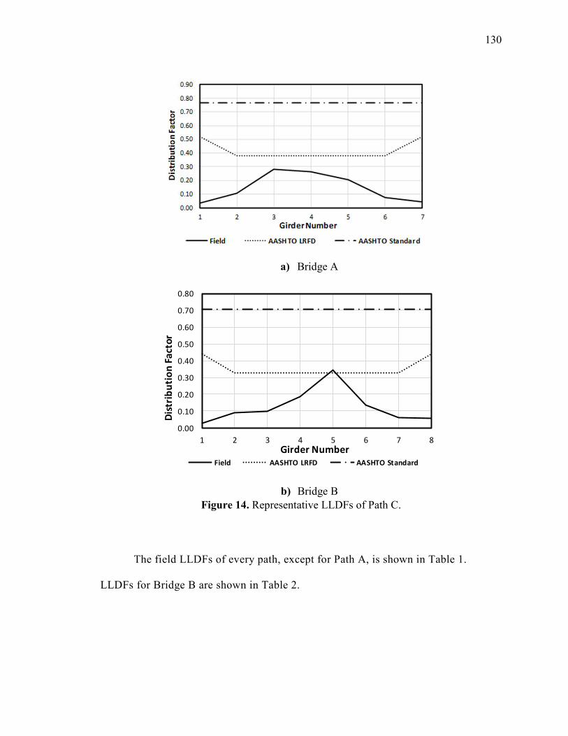
130

a) Bridge A

b) Bridge B

Figure 14. Representative LLDFs of Path C.

The field LLDFs of every path, except for Path A, is shown in Table 1.

LLDFs for Bridge B are shown in Table 2.

0.00

0.10

0.20

0.30

0.40

0.50

0.60

0.70

0.80

1 2 3 4 5 6 7 8

Dis

trib

uti

on

Fa

cto

r

Girder Number


131

Table 1. Field LLDFs for Bridge A

Path G1 G2 G3 G4 G5 G6 G7

Path A* N/A N/A N/A N/A N/A N/A N/A

Path B 0.084 0.270 0.293 0.227 0.079 0.020 0.026

Path C 0.036 0.110 0.282 0.257 0.208 0.071 0.048

Path D 0.018 0.033 0.087 0.209 0.204 0.235 0.214

Path E 0.004 0.021 0.022 0.066 0.141 0.212 0.534

*Data from Path A was lost.

Table 2. Field LLDFs for Bridge B

Path G1 G2 G3 G4 G5 G6 G7 G8

Path A 0.318 0.246 0.171 0.143 0.088 0.021 0.007 0.006

Path B 0.103 0.290 0.154 0.203 0.164 0.047 0.022 0.018

Path C 0.028 0.091 0.098 0.188 0.346 0.134 0.060 0.055

Path D 0.011 0.015 0.034 0.093 0.302 0.198 0.181 0.166

Path E 0.001 0.005 0.011 0.035 0.161 0.166 0.216 0.407

The codified LLDFs from the AASHTO LRFD and AASHTO Standard

specifications are shown in Tables 3 and 4. From the field tests, two field LLDFs

exceed the AASHTO LRFD codified LLDF values.

Table 3. Comparison of Field and Codified LLDFs for Bridge A


G1* 0.084 0.52 0.768

G2 0.27 0.38 0.768

G3 0.293 0.38 0.768

G4 0.257 0.38 0.768

G5 0.208 0.38 0.768

G6 0.235 0.38 0.768

G7 0.534 0.52 0.768


132

Table 4. Comparison of Field and Codified LLDFs for Bridge B


G1 0.318 0.438 0.705

G2 0.290 0.330 0.705

G3 0.171 0.330 0.705

G4 0.203 0.330 0.705

G5 0.346 0.330 0.705

G6 0.198 0.330 0.705

G7 0.216 0.330 0.705

G8 0.407 0.438 0.705

An exterior field LLDF on Bridge A and an interior field LLDF on Bridge B

were higher than the respective codified LLDF. It was found that the damage along

the longitudinal joints between the DT girders was the cause of the exceedingly high

field LLDFs. The joints were damaged sufficiently that the load could not be

distributed transversely as intended. This caused the LLDFs of the girders directly

under the load to increase. More analyses and discussion about the LLDFs of the two

DT bridges can be found in Kidd et al. (2020).

BRIDGE MODELING

Computer Modeling

The field tests proved that the AASHTO LRFD Specifications are generally

conservative for the two tested DT bridges, unless sufficient damage is present.

However, more data is necessary to determine if this is correct for the majority of DT

girders in service. To study this, computer models were made of the two field tested

DT bridges, and they were calibrated to accurately represent the conditions of

133

Bridges A and B. The models were created in CSi Bridge, which has already been

proven to accurately depict the response of a bridge due to a moving load (Torres,

2016; Huang and Davis, 2018). The models were made using solid elements for the

stems of the DT girder and shell elements were used for the flanges. Two-joint link

elements were used to connect the stems to the flanges to make one composite DT

girder. To connect the adjacent DT girders, two-joint links were used between the

DT girder flanges (shell elements). Pin restraints were applied at the bottom of each

stem at the ends of the DT girders, to represent the abutment. A picture of the model

for Bridge A can be seen in Figure 15.

a) Bridge A

134

a) Bridge B

Figure 15. Analytical Model Developed in CSi Bridge

Calibration

Once the model was created using the bridge plans, the models needed to be

calibrated. The DT bridges are 34 and 38 years old, respectively, and have

significant instances of damage. To account for this damage and calibrate the model

with the field strain data, multiple changes to the models were made. Both bridges

were calibrated with the data from Path C of the respective field tests. This is impart

due to the fact that most traffic will be driving down the center of the bridge, similar

to Path C. The shear stiffness of the two-joint links between the DT girders were

modified to represent the damage of the longitudinal joints. Since the bridges has

been in-service for over 30 years, cracking in the DT girders can be expected. Thus,

reduction factor was applied to the modulus of elasticity of the concrete. For Bridge

A, the modulus of elasticity of the concrete in the flanges of the DT girder was not

reduced. However, the concrete in the flanges for Bridge B required a reduction in

modulus of elasticity. Bridge B has a smaller cross-sectional depth and a longer span

135

length than Bridge A. Hence, more cracking would be prevalent in Bridge B. Bridge

B also required another reduction since there was shear cracking in girder G4. G4

was the only girder that received this reduction.

The analytical model was compared to the field data by percent differences.

The equation for percent difference is shown in Equation 7.

Percent Difference �%# � M NOPQRSTUPQ3VTWQXYZ[\]^_`[\ab_c\d

ef ∗ 100 (7)

Table 5 shows the comparison of the analytical LLDFs to the field LLDFs of

Bridge A. The percent differences of the analytical and field LLDFs are within 10%

for most of the girders. The two exceptions are the girders with low LLDFs. The

nature of the percent difference function exaggerates the difference of the two

values, even though the analytical LLDFs are only different by less than two

hundredths.

Table 5. Calibration of LLDFs for Bridge A

G1 G2 G3 G4 G5 G6 G7

Analytical 0.037 0.101 0.257 0.252 0.225 0.092 0.035

Field 0.035 0.108 0.281 0.264 0.205 0.073 0.044

Percent

Difference 5.98 6.73 9.02 4.79 9.49 23.22 22.65

The comparison of the analytical LLDFs to the field LLDFs of Bridge B are

shown in Table 6. Again, the percent differences of the exterior girders are large, but

only because the numbers are so small. The girders that are underneath the truck load

all have percent differences of less than 10%.

136

Table 6. Calibration of LLDFs for Bridge B

G1 G2 G3 G4 G5 G6 G7 G8

Analytical 0.063 0.088 0.104 0.199 0.314 0.137 0.062 0.032

Field 0.028 0.09 0.098 0.189 0.345 0.136 0.059 0.055

Percent

Difference 77.12 1.93 6.35 5.01 9.34 0.59 5.13 52.00

PARAMETRIC STUDY

The calibrated models were then used to conduct a parametric study. The cost and

time to study the LLDFS of DT girder bridges of many different geometries and variables

using field tests is substantial. Therefore, the calibrated models were modified to

represent a variety of different bridges in the field. The parameters that were modified

during this study include: span length, deck width, the location of diaphragms, concrete

strength, and the width-length ratio. The basis for choosing these ranges were based upon

the current DT bridges in South Dakota, since these two cross-sections are standard for

South Dakota bridges. For example, according to the South Dakota Department of

Transportation’s bridge management system, the shortest and longest span of a single

span DT girder bridge is 6.1 meters and 30.5 meters respectively. Each model created

was tested over the same paths as the field tests. Hence, each model had five paths. The

exceptions include when the deck width of the bridge was altered. Paths were added

when the deck width was increased, and paths were removed when the deck width

decreased. However, the path loading the exterior girders was always the suggested 0.61

meters from the edge of the girder, per AASHTO LRFD.

137

RESULTS

Span Length

The span length of the two DT girder bridges was investigated between 6.1

and 30.5 meters. The original in-service bridge is included in this range as well. This

range was chosen because it includes the minimum and maximum span length of DT

bridges in South Dakota.

The change in LLDFs as a function of span length for Bridge A is shown in

Figure 16. Corresponding values are shown in Table 7. The analytical interior LLDFs

decrease at a rate of 10.8% per +6.1 meters, on average. As seen in Figure 16, the

AASHTO LRFD LLDFs match the pattern of the analytical LLDFs and are

conservative. The percent difference varies from 25.7% to 15.8% as the span length

increases. The AASHTO LRFD exterior LLDFs however do not show the same trend

as the analytical LLDFs, since the lever rule does not account for span length. At a

span length of 30.5 meters, the percent difference is 57.7%. This is overly

conservative. The exterior analytical LLDFs decrease at an average rate of 8.1% per

+6.1 meters. The AASHTO Standard is significantly higher than the analytical

LLDFs and AASHTO LRFD LLDFs in all instances.

138

a) Interior LLDFs

b) Exterior LLDFs

Figure 16. Change in LLDFs due to Span Length in Bridge A

139

Table 7. Change in LLDF due to Span Length in Bridge A

a) Interior LLDF

Span

(m)

Max

Int.

LLDF

AASHTO

LRFD Int.

LLDF

AASHTO

Standard

LLDF

6.1 0.380 0.492 0.811

6.86 0.347 0.472 0.811

7.62 0.336 0.455 0.811

11.7 0.303 0.380 0.768

18.3 0.275 0.338 0.736

24.4 0.262 0.308 0.715

30.5 0.245 0.287 0.703

b) Exterior LLDF

Span

(m)

Max

Ext.

LLDF

AASHTO

LRFD Ext.

LLDF

AASHTO

Standard

LLDF

6.1 0.386 0.520 0.811

6.86 0.381 0.520 0.811

7.62 0.374 0.520 0.811

11.7 0.358 0.520 0.768

18.3 0.333 0.520 0.736

24.4 0.297 0.520 0.715

30.5 0.278 0.520 0.703

The change in LLDFs due to the change in span length for Bridge B is shown

in Figure 17. The analytical and two AASHTO design values are shown in Table 8.

The analytical interior LLDFs in Figure 17 are almost identical to the AASHTO

LRFD, until the span length is less than or equal to 12.2 meters. Then, the analytical

interior LLDFs are greater than the AASHTO LRFD values. However, this is due to

the shear crack in girder G4. G4 cannot resist the load of Path C, which transfers

more load to G5. In the analytical study, G5 had the only interior LLDFs that exceed

AASHTO LRFD LLDFs. The interior analytical LLDFs decrease by 8.5% per +6.1

140

meters on average. Similar to Bridge A, the exterior AASHTO LRFD LLDFs do not

match the pattern of the analytical LLDFs. However, the AASHTO LRFD exterior

LLDFs are more accurate, at a span length of 30.5 meters the percent difference is

40%. At a span length of 6.1 meters, the exterior LLDF barely exceeds the AASHTO

LRFD LLDFs. The AASHTO Standard LLDFs continue to be significantly higher,

therefore, discussion including these values will not be included. It is important to

notice that the analytical exterior LLDFs decrease with span length, even when it is

not considered when calculating AASHTO LRFD exterior LLDFs.

a) Interior LLDFs

141

b) Exterior LLDFs

Figure 17. Change in LLDFs Due to Span Length in Bridge B

Table 8. Change in LLDFs due to Span Length in Bridge B

a) Interior LLDF

Span

(m)

Max

Int.

LLDF

AASHTO

LRFD Int.

LLDF

AASHTO

Standard

LLDF

6.1 0.540 0.447 0.747

7.62 0.488 0.414 0.747

9.14 0.447 0.389 0.747

12.2 0.363 0.353 0.721

14.6 0.314 0.330 0.705

18.3 0.307 0.309 0.69

24.4 0.285 0.282 0.674

30.5 0.259 0.263 0.664

142

b) Exterior LLDF

Span

(m)

Max

Ext.

LLDF

AASHTO

LRFD Ext.

LLDF

AASHTO

Standard

LLDF

6.1 0.448 0.438 0.747

7.62 0.435 0.438 0.747

9.14 0.411 0.438 0.747

12.2 0.391 0.438 0.721

14.6 0.327 0.438 0.705

18.3 0.345 0.438 0.69

24.4 0.312 0.438 0.674

30.5 0.292 0.438 0.664

Location of Diaphragms

The location of the diaphragms was varied between no diaphragms, at the

endspans, at the midspan, and both the midspan and endspan. The variation in

LLDFs based on the location of diaphragms on Bridge A is shown in Figure 18. The

data corresponding to Figure 18 can be seen in Table 9. There is no significant

change (≤2%) in maximum LLDFs when diaphragms at the endspan are present.

When diaphragms are present at both endspan and midspan, interior LLDFs increase

and exterior LLDFs decrease. Again, this value is very minimal. It shows yet again

that AASHTO LRFD LLDFs may be too conservative for exterior LLDFs.

143

a) Interior LLDFs

b) Exterior LLDFs

Figure 18. Variation of LLDFs due to Diaphragm Location in Bridge A

0.00

0.10

0.20

0.30

0.40

0.50

0.60

0.70

0.80

0.90

None Endspan Midspan Both

LLD

F

Diaphragm Location

Max Int. LLDF AASHTO Int. LLDF

AASHTO Standard LLDF

0.00

0.10

0.20

0.30

0.40

0.50

0.60

0.70

0.80

0.90


LLD

F

Diaphragm Location

Max Ext. LLDF AASHTO Ext. LLDF


144

Table 9. Change in LLDFs due to Diaphragm Location in Bridge A

a) Interior LLDFs

Diaphragm

Location

Max Int.

LLDF

AASHTO LRFD

Int. LLDF

AASHTO

Standard LLDF

None 0.314 0.33 0.705

Endspan 0.318 0.33 0.705

Midspan 0.319 0.33 0.705

Both 0.298 0.33 0.705

b) Exterior LLDFs

Diaphragm

Location

Max Ext.

LLDF

AASHTO

Ext. LLDF

AASHTO

Standard

LLDF

None 0.358 0.52 0.768

Endspan 0.358 0.52 0.768

Midspan 0.356 0.52 0.768

Both 0.353 0.52 0.768

The same analysis was done on Bridge B, as seen in Figure 19 and Table 10.

When diaphragms are present at the midspan and endspan, both the LLDFs decrease.

Otherwise, there is very little change (6% max) in LLDFs. The presence of

diaphragms at the midspan and endspan changed the LLDFs by a maximum of 15%

and 5% on average. Since this was not as obvious in Bridge A, it suggests that a 584

mm deep DT girder cannot fully transfer the load like a 762 mm deep girder when it

is damaged.

145

a) Interior LLDFs

b) Exterior LLDFs

Figure 19. Variation of LLDFs due to Diaphragm Location in Bridge B

0.00

0.10

0.20

0.30

0.40

0.50

0.60

0.70

0.80


LLD

F

Diaphragm Location

Max Int. LLDF AASHTO Int. LLDF


0.00

0.10

0.20

0.30

0.40

0.50

0.60

0.70

0.80


LLD

F

Diaphragm Location

Max Ext. LLDF AASHTO LRFD Ext. LLDF


146

Table 10. Change in LLDFs due to Diaphragm Location in Bridge B

a) Interior LLDFs

Diaphragm

Location

Max

Int.

LLDF

AASHTO

Int.

LLDF

AASHTO

Standard

LLDF

None 0.314 0.33 0.705

Endspan 0.318 0.33 0.705

Midspan 0.319 0.33 0.705

Both 0.298 0.33 0.705

b) Exterior LLDFs

Diaphragm

Location

Max

Ext.

LLDF

AASHTO

Ext.

LLDF

AASHTO

Standard

LLDF

None 0.327 0.438 0.705

Endspan 0.344 0.438 0.705

Midspan 0.349 0.438 0.705

Both 0.320 0.438 0.705

Deck Width

The deck width was varied by adding or removing DT girders to the existing

bridge. The number of girders varies from 5 to 9. The effect of deck width on LLDFs

for Bridge A can be seen in Figure 20 and Table 11. From the analytical LLDF

values, there is no clear indication of the effect that the deck width has on DT girder

bridges with damage. An interesting result shows that the interior LLDF increases

slightly when nine girders are used. The interior LLDF increases 12% when nine

girders are present. The girder that has this LLDF is the girder that exceeded the

AASHTO LRFD for Bridge A, implying that the longitudinal joint damage is the

reason for this high LLDF.

147

a) Interior LLDFs

b) Exterior LLDFs

Figure 20. Change in LLDFs Due to Deck Width in Bridge A

0.00

0.10

0.20

0.30

0.40

0.50

0.60

0.70

0.80

5 6 7 8 9

LLD

F

Number of Girders

Max Interior LLDF AASHTO LRFD Int. LLDF

AASHTO Standard

0.00

0.10

0.20

0.30

0.40

0.50

0.60

0.70

0.80

5 6 7 8 9

LLD

F

Number of Girders

Max Exterior LLDF AASHTO LRFD Ext. LLDF

AASHTO Standard

148

Table 11. Change in LLDFs Due to Deck Width in Bridge A

a) Interior LLDFs

Number of

Girders

Max Int.

LLDF

AASHTO

LRFD Int.

LLDF

AASHTO

Standard

LLDF

9 0.342 0.38 0.8

8 0.303 0.38 0.787

7 0.303 0.38 0.773

6 0.308 0.38 0.725

5 0.309 0.38 0.718

b) Exterior LLDFs

Number of

Girders

Max Ext.

LLDF

AASHTO

LRFD Ext.

LLDF

AASHTO

Standard

LLDF

9 0.358 0.52 0.8

8 0.364 0.52 0.787

7 0.358 0.52 0.773

6 0.362 0.52 0.725

5 0.362 0.52 0.718

The effect of deck width on the LLDFs for Bridge B can be seen in Figure 21

and Table 12. The AASHTO LRFD are consistent with the analytical LLDFs, both

interior and exterior, but still conservative. The same results occurred as it did in

Bridge A. When the bridge has nine girders the interior LLDF increased by less than

two hundredths. According to the figures and tables, there is no significant

correlation between the number of girders on a DT girder bridge and the LLDFs.

This is logical for a DT with significant longitudinal joint damage. If the load

distribution is poor, then adding more girders would not change LLDFs significantly.

149

a) Interior LLDFs

b) Exterior LLDFs

Figure 21. Change in LLDFs Due to Deck Width in Bridge B

0.00

0.10

0.20

0.30

0.40

0.50

0.60

0.70

5 6 7 8 9

LLD

F

Number of Girders

Max Interior LLDF AASHTO LRFD Int. LLDF


0.00

0.10

0.20

0.30

0.40

0.50

0.60

0.70

5 6 7 8 9

LLD

F

Number of Girders

Max Exterior LLDF AASHTO LRFD Ext. LLDF


150

Table 12. Change in LLDFs Due to Deck Width in Bridge B

a) Interior LLDFs

Deck

Width

Max Int.

LLDF

AASHTO

LRFD Int.

LLDF

AASHTO

Standard

LLDF

9 0.318 0.330 0.715

8 0.314 0.330 0.705

7 0.320 0.330 0.696

6 0.336 0.330 0.686

5 0.312 0.330 0.676

b) Exterior LLDFs

Deck

Width

Max Ext.

LLDF

AASHTO

LRFD Ext.

LLDF

AASHTO

Standard

LLDF

9 0.357 0.438 0.715

8 0.327 0.438 0.705

7 0.324 0.438 0.696

6 0.368 0.438 0.686

5 0.375 0.438 0.676

Concrete Strength

The concrete strength of the DT girders was investigated to see if it impacted

the LLDFs. The LLDFs for Bridge A can be seen in Figure 22 and the corresponding

values in Table 13. The only change that occurred was when the concrete

compressive strength was 41.37 MPa. Both the interior and the exterior LLDFs

increased. However, it only increased by 2.3% and 3.3% respectively. This may

imply that high strength concrete may have higher LLDFs, but for typical

compressive strength values, it has very little effect.

151

a) Interior LLDFs

b) Exterior LLDFs

Figure 22. Change in LLDFs Due to Concrete Strength in Bridge A

0.00

0.10

0.20

0.30

0.40

0.50

0.60

0.70

0.80

0.90

27 30 33 36 39 42

LLD

F

Concrete Strength (MPa)

Max Int. LLDF AASHTO LRFD Int. LLDF


0.00

0.10

0.20

0.30

0.40

0.50

0.60

0.70

0.80

0.90

27 30 33 36 39 42

LLD

F




152

Table 13. Change in LLDFs Due to Concrete Strength in Bridge A

a) Interior LLDFs

f'c

(MPa) Max Int.

LLDF

AASHTO

LRFD INT.

LLDF

AASHTO

Standard

LLDF

27.58 0.303 0.38 0.768

34.47 0.303 0.38 0.768

41.37 0.310 0.38 0.768

b) Exterior LLDFs

f'c

(MPa) Max Ext.

LLDF

AASHTO

LRFD Ext.

LLDF

AASHTO

Standard

LLDF

27.58 0.358 0.52 0.768

34.47 0.358 0.52 0.768

41.37 0.370 0.52 0.768

For Bridge B, the LLDFs of the analytical model and two AASHTO

specifications are shown in Figure 23 and Table 14. There is very minimal changes

between f’C = 41.37 MPa and f’C = 37.92 MPa (<2%). However, when f’C = 27.58

both the interior and exterior LLDFs increased by 2.8% and 3.6% respectively.

Overall, the concrete strength has no significant effect on the LLDFs of DT girder

bridges.

153

a) Interior LLDFs

b) Exterior LLDFs

Figure 23. Change in LLDFs Due to Concrete Strength in Bridge B

0.00

0.10

0.20

0.30

0.40

0.50

0.60

0.70

0.80

25 30 35 40 45

LLD

F


Max Int. LLDF AASHTO LRFD INT. LLDF


0.00

0.10

0.20

0.30

0.40

0.50

0.60

0.70

0.80

25 30 35 40 45

LLD

F




154

Table 14. Change in LLDFs Due to Concrete Strength in Bridge B

a) Interior LLDFs

f'c

(MPa) Max Int.

LLDF

AASHTO

LRFD INT.

LLDF

AASHTO

Standard

LLDF

27.58 0.323 0.33 0.705

37.92 0.314 0.33 0.705

41.37 0.318 0.33 0.705

b) Exterior LLDFs

f'c

(MPa) Max Ext.

LLDF

AASHTO

LRFD Ext.

LLDF

AASHTO

Standard

LLDF

27.58 0.339 0.438 0.705

37.92 0.327 0.438 0.705

41.37 0.324 0.438 0.705

Width-Length Ratio

The effect of the width to length ratio has on the LLDFs is also being

investigated in this study. For Bridge A, this is seen in Figure 24 and Table 15. As

the width to length ratio increases, so does the LLDF. The AASHTO LRFD interior

LLDFs show a similar pattern to the analytical interior LLDFs but are slightly more

conservative. The maximum percent difference is 25.7%. The AASHTO exterior

LLDFs is significantly higher than the analytical exterior LLDFs. The maximum

percent difference between exterior LLDFs and the AASHTO LRFD exterior LLDF

is 72%, which is too conservative.

155

a) Interior LLDFs

b) Exterior LLDFs

Figure 24. Change in LLDFs Due to Width-Length Ratio in Bridge A

156

Table 15. Change in LLDFs Due to Width-Length Ratio in Bridge A

a) Interior LLDF

W/L

Max

Int.

LLDF

AASHTO

LRFD Int.

LLDF

AASHTO

Standard

LLDF

1.40 0.380 0.492 0.811

1.24 0.347 0.472 0.811

1.12 0.336 0.455 0.811

0.90 0.342 0.38 0.800

0.80 0.303 0.38 0.787

0.70 0.303 0.38 0.768

0.60 0.308 0.38 0.757

0.50 0.309 0.38 0.741

0.47 0.275 0.338 0.736

0.34 0.262 0.308 0.715

0.27 0.245 0.287 0.703

a) Exterior LLDFs

W/L

Max

Ext.

LLDF

AASHTO

LRFD Ext.

LLDF

AASHTO

Standard

LLDF

1.40 0.386 0.520 0.811

1.24 0.381 0.520 0.811

1.12 0.374 0.520 0.811

0.90 0.358 0.520 0.800

0.80 0.364 0.520 0.787

0.70 0.358 0.520 0.768

0.60 0.362 0.520 0.757

0.50 0.362 0.520 0.741

0.47 0.333 0.520 0.736

0.34 0.297 0.520 0.715

0.27 0.278 0.520 0.703

The effect of width to length ratio on LLDFs for Bridge B can be found in

Figure 25 and Table 16. Again, both interior and exterior LLDFs increase as the

width-length ratio increases. However, the AASHTO LRFD LLDFs are more

consistent with Bridge B until W/L > 0.766. Then, the interior LLDFs exceed the

157

AASHTO LRFD LLDFs. Again, the shear crack at girder G4 is the cause. G5 is the

only girder to exceed the AASHTO LRFD LLDF values. The exterior AASHTO

LRFD LLDFs are more conservative than the interior LLDFs. Only at a W/L = 1.53

does the analytical LLDF slightly exceed the AASHTO LRFD exterior LLDF.

a) Interior LLDFs

158

b) Exterior LLDFs

Figure 25. Change in LLDFs Due to Width-Length Ratio in Bridge B

Table 16. Change in LLDFs Due to Width-Length Ratio in Bridge B

a) Interior LLDFs

W/L

Max

Int.

LLDF

AASHTO

LRFD Int.

LLDF

AASHTO

Standard

1.53 0.540 0.447 0.747

1.23 0.488 0.414 0.747

1.02 0.447 0.389 0.747

0.766 0.363 0.353 0.721

0.713 0.318 0.330 0.715

0.634 0.314 0.330 0.705

0.554 0.320 0.330 0.696

0.511 0.307 0.309 0.69

0.475 0.336 0.330 0.686

0.396 0.312 0.330 0.676

0.383 0.285 0.282 0.674

0.307 0.259 0.263 0.664

159

b) Exterior LLDFs

W/L

Max

Ext.

LLDF

AASHTO

LRFD Ext.

LLDF

AASHTO

Standard

1.53 0.448 0.438 0.747

1.23 0.435 0.438 0.747

1.02 0.411 0.438 0.747

0.766 0.391 0.438 0.721

0.713 0.328 0.438 0.715

0.634 0.327 0.438 0.705

0.554 0.324 0.438 0.696

0.511 0.345 0.438 0.69

0.475 0.368 0.438 0.686

0.396 0.375 0.438 0.676

0.383 0.312 0.438 0.674

0.307 0.292 0.438 0.664

It is important to notice that the analytical exterior LLDFs decrease with span

length, even when it is not considered when calculating AASHTO LRFD exterior

LLDFs. Even though this analysis shows a trend, it appears that the width-length

ratio is only affecting the LLDF because of the change in span length. It has already

been found that width has little effect. However, the width to length ratio may be a

good indication that bridge rating engineers should investigate the damage and

LLDFs more in-depth.

SUMMARY AND CONCLUSIONS

The purpose of this study was to create an accurate model of two DT girder

bridges with significantly damaged longitudinal joints. To accomplish this goal, strain

data from field tests were used to calibrate the two models developed on CSi Bridge.

160

Calibration of the models involved reducing the shear stiffness of the link elements

between girders and reducing the modulus of elasticity due to cracking in the concrete.

Once the models were calibrated, a parametric study was conducted to identify the effect

that different parameters have on the LLDFs. The parameters investigated were span

length, diaphragm location, deck width, concrete strength, and width-length ratio. Then,

the analytical LLDFs can be compared to the AASHTO LRFD LLDFs and AASHTO

Standard LLDFs to identify the accuracy of the codified LLDF equations. Based on the

content in this paper, the following conclusions were made for DT girder bridges with

significant longitudinal joint damage.

1. The AASHTO LRFD interior LLDFs were typically consistent with the analytical

interior LLDFs, if not conservative for DT girder bridges with significant

longitudinal joint damage. When Bridge B had small spans (i.e. less than 12.2

meters), the AASHTO LRFD interior LLDFs were not sufficiently conservative.

The AASHTO LRFD exterior LLDFs were conservative for the DT girder bridges

with significant longitudinal joint damage. The AASHTO Standard LLDFs were

over-conservative for all cases investigated during this parametric study.

2. The concrete strength, deck width, and diaphragm location did cause some

variation in LLDFs but the values were not significant. When diaphragms were

present at the endspan and midspan, there was some variation (5% on average). It

is reasonable to conclude theses parameters do not have a significant effect on the

LLDFs of a DT girder bridge with significant joint damage.

3. Both the interior and exterior LLDFs decrease as the span length increases. The

interior LLDF decreased by 10.8% per 6.1 m of span, on average for Bridge A.

161

The exterior LLDF decreased by 8.1% per 6.1 m of span, on average. The interior

LLDF decreased by 8.5% per 6.1 m of span, on average for Bridge B. The

exterior LLDF decreased by 5.8% per 6.1 m of span, on average for Bridge B.

This is in agreement with previous studies and the AASHTO LRFD interior

LLDF equation. However, the AASHTO LRFD exterior LLDFs do not decrease

with span length since the lever rule is used. This may be an over-conservative

approach.

4. The width-length (W/L) ratio did show an impact on the LLDFs. However,

considering the deck width did not affect the LLDFs, it is reasonable to believe

that this impact was due to the change in span length not specifically the width-

length ratio. At a W/L larger than 0.766 on Bridge B, the interior LLDFs

exceeded AASHTO LRFD LLDFs due to a shear crack in one of the girders. W/L

may be an important indicator to bridge rating engineers to evaluate the load-

carrying capacity using LLDFs for deteriorating DT bridges.

ACKNOWLEDGEMENTS


Department of Transportation (SDDOT) and the Mountain-Plains Consortium (MPC), a




authors, who are responsible for the facts and accuracy of the information presented. The

162

research team is grateful for all those who participated in the field tests yield the data

used in this paper.

163

REFERENCES

AASHTO LRFD. (2012). “AASHTO LRFD Bridge Design Specifications, Sixth


(AASHTO), Washington, DC.

AASHTO Standard. (1996). “Standard Specifications for Highway Bridges, Sixteenth


(AASHTO), Washington, D.C.

Culmo, M. P., and Seraderian, R. L. (2010). “Development of the northeast extreme tee

(NEXT) beam for accelerated bridge construction.” PCI J., 55(3), 86–101.

Huang, J., and Davis, J. (2018). “Live load distribution factors for moment in next beam

bridges.” Journal of Bridge Engineering, 23(3), 06017010. Seo, J., and Hu, J. W.

(2014). “Simulation-based load distribution behaviour of a steel girder bridge

under the effect of unique vehicle configurations.” European Journal of

Environmental and Civil Engineering, 18(4), 457-469.





distribution for timber bridges.” Journal of Bridge Engineering, 22(11),

04017085.




164



concrete composite bridges under farm traffic.” Engineering Structures, 69, 72-

82.


next beam bridges" Masters Theses - February 2014.

Tazarv, M., Bohn, L., Wehbe, N. (2019). “Rehabilitation of longitudinal joints in double-

tee bridges,” Journal of Bridge Engineering, ASCE, DOI:

10.1061/(ASCE)BE.1943-5592.0001412, 15 pp.

Torres, Victor J., (2012). "Live load testing and analysis of a 48-year-old double tee

girder bridge." Master’s Thesis.

Wehbe, N., Konrad, M., and Breyfogle, A. (2016). “Joint Detailing Between Double Tee

Bridge Girders for Improved Serviceability and Strength.” Transportation

Research Record: Journal of the Transportation Research Board, No. 2592,

Transportation Research Board of the National Academies, Washington, D.C.



12(6), 765–773.

Zokaie, T. (2000). “AASHTO-LRFD Live Load Distribution Specifications.” Journal of

Bridge Engineering, 5(2).

Field and Numerical Study for Deteriorating Precast Double ...

Documents