Field and laboratory investigations of runout distances of debris flows in the Dolomites (Eastern Italian Alps)

Geomorphology 115 (2010) 294–304

Contents lists available at ScienceDirect

Geomorphology

j ourna l homepage: www.e lsev ie r.com/ locate /geomorph

Field and laboratory investigations of runout distances of debris flows in theDolomites (Eastern Italian Alps)

Vincenzo D'Agostino a,⁎, Matteo Cesca a,1, Lorenzo Marchi b,2

a Department of Land and Agro-Forest Environments, University of Padova, Agripolis, Viale dell'Università 16, 35020 Legnaro (Padova), Italyb CNR-IRPI, Corso Stati Uniti 4, 35127 Padova, Italy

⁎ Corresponding author. University of Padova, DepartEnvironments, Agripolis, Viale dell'Università 16, 350200498272682; fax: +39 0498272686.

E-mail addresses: [email protected] (V. [email protected] (M. Cesca), lorenzo.marchi@irpi.

1 Tel.: +39 0498272700; fax: +39 0498272686.2 Tel.: +39 0498295825; fax: +39 0498295827.

0169-555X/$ – see front matter © 2009 Elsevier B.V. Adoi:10.1016/j.geomorph.2009.06.032

a b s t r a c t

Article history:Received 22 December 2007Received in revised form 30 April 2008Accepted 15 June 2009Available online 18 July 2009

Keywords:Alluvial fanDebris flowRunout distanceLaboratory flumeAlps

The estimation of runout distances on fans has a major role in assessing debris-flow hazards. Different methodshave been devised for this purpose: volume balance, limiting topographic methods, empirical equations, andphysical approaches. Data collected from field observations are the basis for developing, testing, and improvingpredictive methods, while laboratory tests on small-scale models are another suitable approach for studyingdebris-flow runout under controlled conditions and for developing predictive equations. This paper analyses theproblemof assessing runout distance, focusingon six debrisflows thatwere triggeredon July 5th, 2006by intenserainfall near Cortina d'Ampezzo (Dolomites, north-eastern Italy). Detailed field surveys were carried outimmediately after the event in the triggering zone, along the channels, and in the deposition areas. A fine-scaledigital terrain model of the study area was established by aerial LiDAR measurements. Total travel and runoutdistances on fansmeasured in thefieldwere comparedwith the results of formulae from the literature (empirical/statistical and physically oriented), and samples of sediment collected from deposition lobes were used forlaboratory tests. The experimental device employed in the tests consists of a tiltingflumewith an inclination from0° to 38°, onwhich a steel tank with a removable gate was installed at variable distances from the outlet. A finalhorizontal planeworks as thedeposition area. Samples of different volumesandvariable sediment concentrationswere tested. Multiple regression analysis was used to assess the length of the deposits as a function of both thepotential energy of the mass and the sediment concentration of the flow. Our comparison of the results oflaboratory tests with field data suggests that an energy-based runout formulamight predict the runout distancesof debris flows in the Dolomites.

© 2009 Elsevier B.V. All rights reserved.

1. Introduction

Debris flows are one of the most important formative processes ofalluvial fans under various climatic conditions. They can transport anddeposit large amounts of water and solid material in short timeintervals, creating a major hazard for people and structures.

The assessment of runout distance, i.e. the length travelled on analluvial fan by a debris flow from the initiation of the deposits untiltheir lowest point, is of utmost importance for delineating the areas atrisk from debris flows. Another key parameter in debris-flow studies isthe total travel distance (the distance from the initiation of the debrisflow to the lowest point of deposition). Methods for determining

ment of Land and Agro-ForestLegnaro (PD), Italy. Tel.: +39

'Agostino),cnr.it (L. Marchi).

ll rights reserved.

debris-flow runout distance and total travel distance can be based onfield data as well as on data generated by physical models. Bycombining these two sources of data, a promising approach emergesfor refining the methods for assessing runout distance on alluvial fans.

This paper contributes to the assessment of debris-flow runoutdistance on fans and total travel distance by integrating fieldmeasurements and laboratory tests on a tilting plane rheometer. Thestudy methods were applied to six debris flows of the Dolomites(eastern Italian Alps). Field surveys and a hydrological analysis madeit possible to assess the principal parameters relevant for the analysisof runout distance. Samples taken from the debris-flow deposits wereused to analyse the depositional processes on the tilting planerheometer; both quasi-static tests of fan formation and dynamic testsusing a flumewere carried out. Field data on runout distance and totaltravel distance were compared with both empirical–statistical anddynamic methods for runout assessment, and with predictiveequations developed from the laboratory test.

This paper is divided into seven sections. Section 2 describes theprincipal methods available for assessing runout distance and totaltravel distance. Section 3 presents the study area, the field surveys, andthe hydrological analysis implemented for assessing the main variables

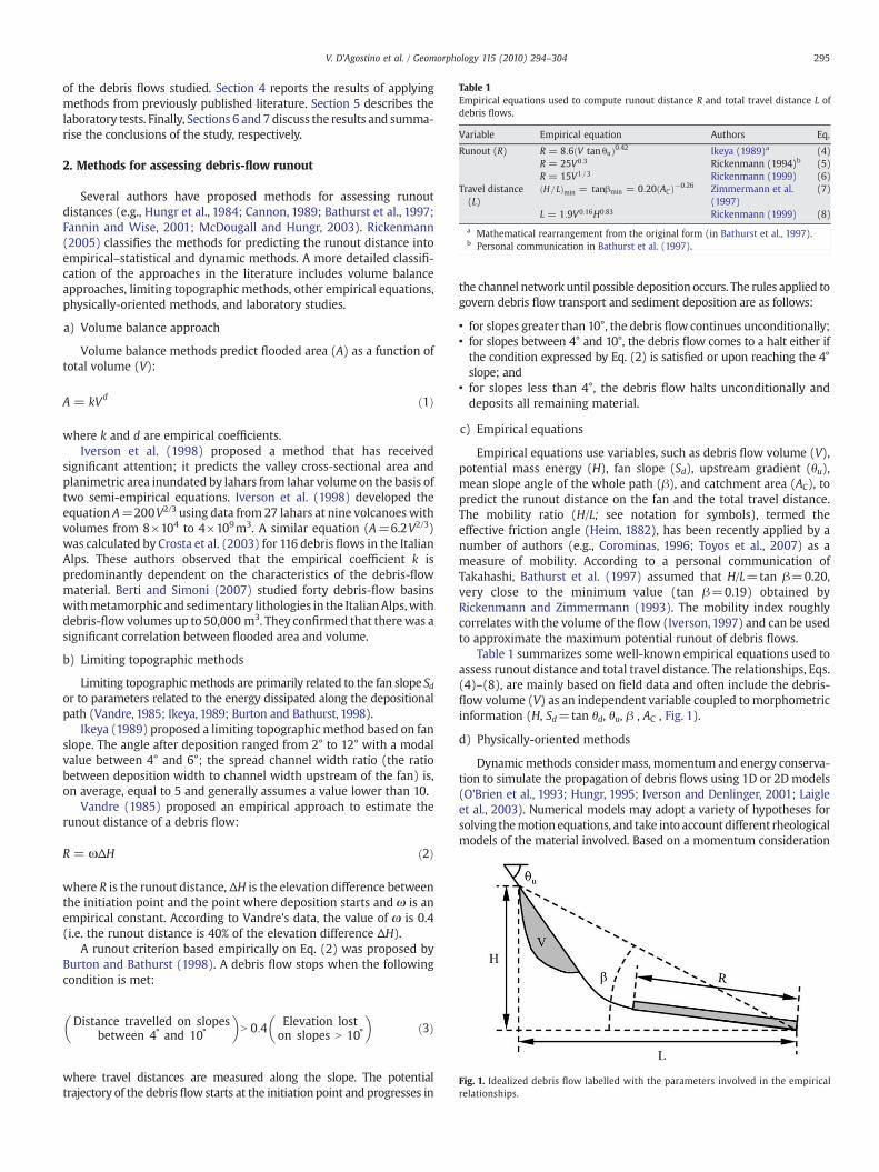
Table 1Empirical equations used to compute runout distance R and total travel distance L ofdebris flows.

Variable Empirical equation Authors Eq.

Runout (R) R = 8:6ðV tan θuÞ0:42 Ikeya (1989)a (4)R = 25V0:3 Rickenmann (1994)b (5)R = 15V1 =3 Rickenmann (1999) (6)

Travel distance(L)

ðH=LÞmin = tanβmin = 0:20ðACÞ−0:26 Zimmermann et al.(1997)

(7)

L = 1:9V0:16H0:83 Rickenmann (1999) (8)

a Mathematical rearrangement from the original form (in Bathurst et al., 1997).b Personal communication in Bathurst et al. (1997).

Fig. 1. Idealized debris flow labelled with the parameters involved in the empiricalrelationships.

295V. D'Agostino et al. / Geomorphology 115 (2010) 294–304

of the debris flows studied. Section 4 reports the results of applyingmethods from previously published literature. Section 5 describes thelaboratory tests. Finally, Sections 6 and 7 discuss the results and summa-rise the conclusions of the study, respectively.

2. Methods for assessing debris-flow runout

Several authors have proposed methods for assessing runoutdistances (e.g., Hungr et al., 1984; Cannon, 1989; Bathurst et al., 1997;Fannin and Wise, 2001; McDougall and Hungr, 2003). Rickenmann(2005) classifies the methods for predicting the runout distance intoempirical–statistical and dynamic methods. A more detailed classifi-cation of the approaches in the literature includes volume balanceapproaches, limiting topographic methods, other empirical equations,physically-oriented methods, and laboratory studies.

a) Volume balance approach

Volume balance methods predict flooded area (A) as a function oftotal volume (V):

A = kVd ð1Þ

where k and d are empirical coefficients.Iverson et al. (1998) proposed a method that has received

significant attention; it predicts the valley cross-sectional area andplanimetric area inundated by lahars from lahar volume on the basis oftwo semi-empirical equations. Iverson et al. (1998) developed theequation A=200V2/3 using data from 27 lahars at nine volcanoes withvolumes from 8×104 to 4×109m3. A similar equation (A=6.2V2/3)was calculated by Crosta et al. (2003) for 116 debris flows in the ItalianAlps. These authors observed that the empirical coefficient k ispredominantly dependent on the characteristics of the debris-flowmaterial. Berti and Simoni (2007) studied forty debris-flow basinswithmetamorphic and sedimentary lithologies in the ItalianAlps,withdebris-flow volumes up to 50,000 m3. They confirmed that therewas asignificant correlation between flooded area and volume.

b) Limiting topographic methods

Limiting topographicmethods are primarily related to the fan slope Sdor to parameters related to the energy dissipated along the depositionalpath (Vandre, 1985; Ikeya, 1989; Burton and Bathurst, 1998).

Ikeya (1989) proposed a limiting topographic method based on fanslope. The angle after deposition ranged from 2° to 12° with a modalvalue between 4° and 6°; the spread channel width ratio (the ratiobetween deposition width to channel width upstream of the fan) is,on average, equal to 5 and generally assumes a value lower than 10.

Vandre (1985) proposed an empirical approach to estimate therunout distance of a debris flow:

R = ωΔH ð2Þ

where R is the runout distance, ΔΗ is the elevation difference betweenthe initiation point and the point where deposition starts and ω is anempirical constant. According to Vandre's data, the value of ω is 0.4(i.e. the runout distance is 40% of the elevation difference ΔH).

A runout criterion based empirically on Eq. (2) was proposed byBurton and Bathurst (1998). A debris flow stops when the followingcondition is met:

Distance travelled on slopesbetween 4˚ and 10˚

� �N 0:4 Elevation lost

on slopes N 10˚

� �ð3Þ

where travel distances are measured along the slope. The potentialtrajectory of the debrisflowstarts at the initiationpoint and progresses in

the channel network until possible deposition occurs. The rules applied togovern debris flow transport and sediment deposition are as follows:

• for slopes greater than 10°, the debris flow continues unconditionally;• for slopes between 4° and 10°, the debris flow comes to a halt either ifthe condition expressed by Eq. (2) is satisfied or upon reaching the 4°slope; and

• for slopes less than 4°, the debris flow halts unconditionally anddeposits all remaining material.

c) Empirical equations

Empirical equations use variables, such as debris flow volume (V),potential mass energy (H), fan slope (Sd), upstream gradient (θu),mean slope angle of the whole path (β), and catchment area (AC), topredict the runout distance on the fan and the total travel distance.The mobility ratio (H/L; see notation for symbols), termed theeffective friction angle (Heim, 1882), has been recently applied by anumber of authors (e.g., Corominas, 1996; Toyos et al., 2007) as ameasure of mobility. According to a personal communication ofTakahashi, Bathurst et al. (1997) assumed that H/L=tan β=0.20,very close to the minimum value (tan β=0.19) obtained byRickenmann and Zimmermann (1993). The mobility index roughlycorrelates with the volume of the flow (Iverson,1997) and can be usedto approximate the maximum potential runout of debris flows.

Table 1 summarizes somewell-known empirical equations used toassess runout distance and total travel distance. The relationships, Eqs.(4)–(8), are mainly based on field data and often include the debris-flow volume (V) as an independent variable coupled tomorphometricinformation (H, Sd=tan θd, θu, β , AC , Fig. 1).

d) Physically-oriented methods

Dynamicmethods considermass, momentum and energy conserva-tion to simulate the propagation of debris flows using 1D or 2Dmodels(O'Brien et al., 1993; Hungr, 1995; Iverson and Denlinger, 2001; Laigleet al., 2003). Numerical models may adopt a variety of hypotheses forsolving themotion equations, and take into account different rheologicalmodels of the material involved. Based on a momentum consideration

296 V. D'Agostino et al. / Geomorphology 115 (2010) 294–304

for aflow travellingover a surfacewith constant slope, the runout lengthR can be described by the following theoretical equation developed byHungr et al. (1984) and Takahashi (1991):

R =fuu cosðθu−θdÞ½1 + ðghu cosθuÞ=ð2u2

uÞ�g2g ðSf cosθd− sinθdÞ

ð9Þ

where θd=the terrain slope angle along the area of deposition, θu=the entry channel slope angle, uu=entry velocity, hu=entry flowdepth, and Sf=the friction slope, which is assumed to be constantalong the runout path and accounts only for sliding friction. Themodelassumes a constant discharge from upstream and no change in flowwidth after the break in slope.

Hungr et al. (1984) assumed the friction slope angle of 10° andreported a good agreement between observed values of R and thosepredicted by Eq. (9) for five debris flows in western Canada. However,when Eq. (9) is applied to 14 debris flows in Japan usingmeasured flowquantities (Okuda and Suwa,1984), better predictions of R are obtainedfor Sf= f tan θd (with f=1.12) rather than arctan (Sf )=10°. Theapplication of Eq. (9) to Swiss debris flows from 1987 (Rickenmann,2005) also predicts reasonable runout lengths using Sf=1.08 tan θd,when observed flow depths are used to estimate the entry velocity uu.For the back analysis of the Japanese and Swiss data, itwas assumed thatthemain surge travelled in the existing channel on the fan to the lowestpoint of deposition with essentially no change in flow width.

e) Laboratory studies

Post-event surveys allow researchers to detect only debris-flowfeatures visible after the end of the processes, such as erosional scars,

Fig. 2. Location of the study area with rock ba

flow marks, and deposits. Field monitoring in instrumented areas is aninvaluableway togatherdataondebris-flowdynamics (Okudaet al.,1980;Genevois et al., 2000; Arattano andMarchi, 2008; Hürlimann et al., 2003).However, field monitoring of debris flows is expensive and time-consuming, and is only convenient for sites that show both a highfrequency of events and favourable logistical conditions. To overcomethese issues, several authors have used laboratory flumes (small-scalemodel experiments) in order to simulate debris-flow deposition(Mizuyama and Uehara, 1983; Van Steijn and Coutard, 1989; Liu, 1996;Deganutti et al., 2003; Ghilardi et al., 2003). Quantities such as flowvelocity, the shape of deposits, deposited volume, and grain-sizedistribution can be measured and controlled in the laboratory tests.Problemsof scale are relevant for physically simulating these phenomena:with only a few exceptions (for example the USGS experimental debris-flow flume, 95 m long and 2 mwide; Major, 1997), channels are typicallynarrower than 0.5 m and up to a few meters long; the volume of sourcematerial is generally lower than0.1 m3, anddebrismixturesarecommonlyrestricted to clay, sand, ormuddysand slurries. This notwithstanding, testsin laboratory flumes make it possible to analyse the relations betweenphysical variables of debrisflowsunder controlled conditions, andprovideuseful data for developing and testing predictive methods.

3. Case study: Fiames debris flows of July 5th, 2006

3.1. Study area

The debris flow studied in this paper occurred in Fiames, a localityof the Dolomites (eastern Italian Alps), near the town of Cortina

sins and debris-flow deposits highlighted.

297V. D'Agostino et al. / Geomorphology 115 (2010) 294–304

d'Ampezzo. An intense rainstorm triggered six debris flows in theafternoon of July 5th, 2006.

Three main morphological units can be identified in the study area(shown in Fig. 2). Rock basins, composed of dolomite, are present in theupper part. A thick talus, consisting of particles from silt to boulders (upto 1–2 m in size), is situated below the rock cliffs (Figs. 3, 4). The lowerpart of the slope is occupied by coalescing fans built by debris flows,whose initiation points are located at the contact between the rock cliffsand the scree slope (Fig. 4).

The areas of the rock basins range from 0.024 to 0.182 km2, themaximum elevations are between 1984 and 2400 ma.s.l., and the mini-mum elevations, which correspond to the initiation areas of the debrisflows, are between 1521 and 1624 ma.s.l. The channel lengths varybetween 110 and 540 m and the mean channel slope between 22° and28°. The climatic conditions are typical of an alpine environment: theannual precipitation at Cortina d'Ampezzo ranges between 900 and1500 mm, with an average of 1100 mm. Snowfall occurs normally fromOctober to May, and intense summer thunderstorms are common andconstitute a maximum in the seasonal precipitation regime.

Fig. 4. Debris-flow channel close to the triggering area (basin 3).

3.2. Field surveys

Immediately after the debris flows of July 2006, field surveys werecarried out in the study area. These field surveys made it possible tomeasure several features of debris-flow deposits: mean and max-imum depth, depths and slopes of deposition lobes, and cross-sectionsof the deposits (Fig. 3). Moreover, cross-sections weremeasured alongthe main channel and detailed descriptions of debris-flow initiationareas were made (Fig. 4). The grain size distribution was assessed:i) bymeans of transect-line measurements on the surfaces of terminaldeposition lobes (84% finer than 0.09 m for the finest sample and0.17 m for the coarsest); ii) by direct measurements of the largestdeposited boulders (1.0 to 1.4 m; intermediate axis); and iii) byprocessing photographs of vertical trenches and assessing theproportion of sediments with diameters finer than 2 cm (estimatedrange from 25 to 40% by weight). The boundaries of the debris-flowdeposits were mapped using a hand-held GPS; the other geometriccharacteristics were measured using a laser range finder and a tape.

Fig. 3. Debris-flow depos

LiDAR and photographic data were acquired from a helicopterflying at an average altitude of 1000 m above ground level duringsnow free conditions in October 2006. The flying speed was 80kn, thescan angle was 20°, and the scan rate was 71KHz. The survey design

ition area (basin 5).

Table 2Basin areaAC, deposited volumeV, planimetric flooded areaA, mean thicknessh (volumeVdivided by the area of deposition), maximum debris-flow sediment concentrationat equilibrium conditions ce max and ‘hydrologic’ estimation of the debris-flow peakdischarge Qd max for each basin; [Qd max] is computed with the Mizuyama et al. (1992)equation: [Qd max]=0.0188V0.79.

Basin Ac (km2) V (m3) A (m2) h (m) ce max (−) Qd max

(m3s−1)[Qd max](m3s−1)

1 0.182 15,000 10,116 1.39 0.665 32 372 0.087 10,600 8543 1.19 0.700 21 283 0.147 46,800 16,934 2.57 0.710 100 924 0.092 11,000 6785 1.50 0.700 22 295 0.091 5200 4609 1.00 0.630 12 166 0.024 2100 3751 0.50 0.725 16 8

Table 3Main topographic characteristics of the Fiames case study: channel length LC and meanwidth Bc, upstream channel slope θu, slope of depositional zone θd, average slope angleof the whole path β, sloped runout length R, horizontal travel distance L and associatedtotal drop H, and estimated peak velocity uu of the surge in the channel.

Basin LC(m)

BC(m)

θu(°)

θd(°)

β(°)

R(m)

L(m)

ΔH(m)

H(m)

uu(m/s)

1 109 15.5 23.3 19.3 20.1 394 472 43 173 4.172 241 11.7 21.9 16.2 18.2 427 634 90 209 3.893 539 9.9 21.9 16.0 19.7 312 800 201 287 6.934 189 12.2 23.0 21.2 21.9 329 481 74 193 3.965 144 12.5 21.6 21.4 21.5 129 254 53 100 3.156 238 6.04 27.9 25.9 27.0 183 375 111 191 4.78

298 V. D'Agostino et al. / Geomorphology 115 (2010) 294–304

point density was specified to be greater than 5 points per m2. LiDARpoint measurements were filtered into returns from vegetation andbare ground using TerrascanTM software classification routines andalgorithms. A comparison between LiDAR and ground GPS elevationpoints carried out in a neighbouring basin showed a vertical accuracyof 0.1 m.

3.3. Event reconstruction

The debris flows of July 5th, 2006 were triggered by an intensethunderstorm and hailstorm from 6 p.m. to 7 p.m. (Central EuropeanSummer Time). The highest values of rainfall intensity during theevent were 12.5 mm/5 min and 64 mm/h. These values weremeasured at a meteorological station located about 1 km from thestudy area and are the highest values ever measured at this stationsince it began operating in 1984. After the event, many hailstonescovered the slopes for about 2h. The debris flows blocked the NationalRoad and a bicycle trail (located on a former railway track) (Fig. 2).Local low slopes next to the bicycle trail and the National Road helpedslow down and deposit the debris flows.

The debris flows initiated at the outlet of the rock basins by themobilization of loose debris into a flow with progressive entrainmentof debris from channel bank erosion and bed scour (Fig. 4). The mainchannel stopped (between 1441 and 1553 ma.s.l.) where the slopeangle decreases and the depositional zone starts.

The deposited volumewas assessed by subtracting the 5meter griddigital terrain model of the deposits (LiDAR data) from the pre-eventtopographic surface, fitted from a topographic map at a scale of1:5000. The results were checked at sample areas in the field and avertical accuracy of 0.10 m was inferred.

Water runoff from the rock basins was simulated by means of akinematic hydrological model that integrates the US Soil ConservationService-Curve Number (SCS-CN) method (Soil Conservation Service,1956, 1964, 1969, 1971, 1972, 1985, 1993) with a geomorphologic unithydrograph (Chow et al., 1988). The SCS-CNmethod is one of themostpopular methods for assessing direct surface runoff from rainfall datathrough a weighted value of the CN parameter of the basin. Theadopted unit hydrograph is extracted from the hypsographic curve byassuming equivalence between the contour lines and lines with thesame concentration time (Viparelli, 1963). We calculated thecorresponding CN values on the basis of the geological setting andland use of the six basins upstream of the triggering point (SoilConservation Service, 1993). Under normal antecedent moistureconditions, the obtained CN values are around CN=85. The secondSCS parametric variable to compute surface runoff involves initialabstraction, accounting for depression storage, interception, andinfiltration before runoff begins. Its value was set to 10% of potentialmaximum retention (directly expressed by the CN) following thesuggestion of Aron et al. (1977) and the assumption of Gregoretti andDalla Fontana (2008) in the hydrologic modelling of headwater basinsof the Dolomites. The concentration time was evaluated as the ratiobetween the main channel length and the flow velocity along theslopes (assumed to be equal to 2 m/s).

Subsequently, the following relation was adopted for assessingdebris-flowdischarge from thewaterflooddischarge (Takahashi,1978):

Qd =Qw

1−cec⁎

ð10Þ

where Qd is the debris-flow discharge associated with the liquiddischargeQw, and c⁎ and ce are the “in situ” volumetric concentrations ofbed sediments before the flood and the debris-flow sedimentconcentration at equilibrium conditions, respectively. Eq. (10) refers toa debris flow generated by sudden release of Qw from the upstream endof an erodible and saturated grain bed. The assumption in Eq. (10) of a

constant ratio ce/c* for the entire duration of the flood would be toosevere a hypothesis in relation to the type of debris-flow surges observedin the streamsof theDolomites (D'Agostino andMarchi, 2003). Therefore,the debris-flow graph was computed from the hydrograph plotted,assuming a linear variation of ce/c* in Eq. (10) from a minimum (ce min=0.2) to amaximumvalue (cemax in correspondence toQwat the peak). Theconcentration ce maxwas calibrated tomatch the sediment volumes of thedebris-flowdeposits estimated bymeans of the LiDAR data and it resultedin a range of 0.63–0.72 (mean of 0.69). Table 2 also reports, for eachcatchment, the basin area AC, the deposited volume V, the flooded area A,themean thicknessh, the debris-flow sediment concentration at the peak(ce max) and the corresponding debris-flow discharge Qd max. The meanthickness of the debris-flow deposits is the ratio between the depositedvolume and the flooded area.

Table 3 presents the main geometric features related to the runoutand the channel reach bounded by the debris-flow triggering pointand the cross-section where deposition starts.

4. Application of runout and travel distance prediction methods

Themethods for assessing runout length and travel distancedescribedin Section 2 of this paper were applied to the field data of the Fiamesdebris flows. The results are discussed in the following paragraphs.

a) Volume balance approach

Using the scheme of Eq. (1), we computed an empirical mobilityrelationship for the Fiames debris flows (Fig. 5); the relationshipdisplays high coefficient of determination (R2=0.92) and has a valueof k equal to to 14.2 for d=2/3. According to Crosta et al. (2003) andBerti and Simoni (2007), k is almost constant in each lithologicalcontext and reflects yield stress and mobility of the flowing mass.

b) Limiting topographic methods

The debris flows of Fiames decelerate and stop at slopes higher(Table 3) than those assumed by themethods proposed by Ikeya (1989)and Burton and Bathurst (1998). Neither method is applicable to theFiames case study. Suchbehaviour can be ascribed to a highly dissipative

Fig. 7. Comparison of travel distances observed in the field with those calculated usingthe relationships shown in Table 1 for the six studied debris flows.

Fig. 5. Relationship between debris-flow volume and flooded area.

299V. D'Agostino et al. / Geomorphology 115 (2010) 294–304

debrisflowand large roughness of the terrain. Applying Eq. (2) producesnonphysical R values (1/4 to 1/20 of observations), because the partialdrop ΔΗ measured in the field is very limited (Table 3).

c) Empirical equations

Eq. (5) tends to overestimate the runout distance, so it can be deemedconservative in the dolomitic environment (Fig. 6). The recalibratedRickenmann (1999) formula (Eq. 6) gives fairly satisfactory results, but itunderpredicts thedistances in two cases. The Ikeya (1989) relation (Eq. 4)shows a similar pattern (Fig. 6), but it has a more marked tendency tounderestimate R. These findings are not surprising, because even thoughEq. (4) is usually applied in different topographic conditions, Ikeya (1989)suggested its use when the top portion of the fan is less than 8°, whereasthe Fiames alluvial fans are much steeper (Table 3).

The empirical equations for assessing total travel distance agreewell with observed values (Fig. 7). Eq. (7) in particular provides acorrect estimate of the measured values in the study area. Consideringthe high fan slope and the L observed values, it is likely that therheology expresses high basal shear stresses. Eq. (8) also gives valuesthat agree fairly well, but it is implicit and the results are too positivelyaffected by the use of observed H values.

d) Physically-oriented methods

The application of Eq. (9) requires that there be no significantchange in flow width moving from the entry channel to the fan area.The observed depositional formsmake this condition possible (Fig. 2);it is also supported by the fact that deposits are elongate with a spreadwidth to runout length ratio close to 0.15.

Fig. 6. Comparison of runout distances observed in the field with those calculated usingthe relationships shown in Table 1 for the six studied debris flows.

In order to calibrate Eq. (9) with the data in Tables 2 and 3, wemust first make a preliminary computation of the entering velocity uuand the assessment of Sf or the parameter f if we set Sf= f tan θd. Weevaluated uu for the peak discharges (Table 2) using the Chézy equation(uu=C g1/2 hu

1/2 sinθu1/2; C=dimensionless Chézy's roughness) adaptedto thesurgemotionofdebrisflows(Rickenmann,1999).Gregoretti (2000)analyzed theneighbouringbasinofAcquabona (Genevois et al., 2000) andcame up with a C value close to 3 when the ratio of flow depth tointermediate diameter of the front sediments is less than 3 and thechannel bed is not congested with loose debris before the surge transit(both conditions agree with the Fiames event). After computing uu withC=3 (Table 3), the iterative solution of Eq. (9) for the unknown Sf, whereR is the measured runout distance, gives six f values in the range 1.016–1.072, with a mean value f=1.030. The relationship can be adequatelycalibrated, but is too sensitive to f variations to the third decimal placewhen, as in our case study, the upstream slope θu and the fan slope θd arevery close.

5. Laboratory tests

Twenty-nine tests were carried out using a tilting-plane rheometer(Fig. 8a): twenty tests simulated the quasi-static formation of a fan, andthe remaining nine examined dynamic fan formation by the means of aflume.

5.1. Experimental device

The physical model consists of a 2 m×1m tilting plane with aninclination(α)between0°and38°, onwhicha steel tankwitha removablegatewas installed. Afixedhorizontal plane (1.5 m×1m),with an artificialroughness (Fig. 8b) to simulate the natural basal friction, served as thedeposition area.

The quasi-static tests of fan formation were performed by installingthe tank at the lower end of the tilting plane, i.e. without a flume (Fig. 8a).The steel tank, with a removable gate facing the deposition plane, is aparallelepipedwith a square base (15 cm×15 cm; 33 cmhigh) andwith amaximum usable volume of 7 dm3.

Dynamic fan formation was simulated using an artificial flumeinstalled on the tilting plane (Fig. 9).

The width of the flume is 0.15 m, and it is between 0 and 180 cmlong, depending on the tank position. The artificial channel bottom iscomposed of a steel plate with an artificial roughness (Fig. 10a); fourdatum lines were painted on the bottom (Fig. 10b).

Fig. 8. (a) Tilting-plane rheometer: set-up for quasi-static tests. (b) Detail of the horizontal plane with artificial roughness (thickness 2 mm).

300 V. D'Agostino et al. / Geomorphology 115 (2010) 294–304

5.2. Tests

The laboratory tests were carried out using debris-flow matrixcollected from lobes in the Fiames fan area. This matrix corresponds,on average, to 30% by weight of the field deposits. In the laboratorytests, samples of debris-flow matrix with maximum diameters up to19 mm were used (Fig. 11); fine material (b0.04 mm) amounts to28.6%. The tested material has a density of 2.55 g/cm3, a porosity of25%, an angle of friction of 40° and a mean diameter of 2.14 mm.

Eight quasi-static simulations were performed using a constanttotal volume of 3 dm3 to simulate solid concentrations by volume of45% and 50%; in the remaining twelve quasi-static tests, a constantsolid volume of 3 dm3 was used, and varying amounts of water wereadded to obtain solid concentrations by volume of 55%, 60%, and 67%.The gradients of the tilting plane were 0°, 5°, 10°, and 15°. In the ninedynamic runs, a constant total volume of 5.5 dm3 was used and thesolid concentrations by volume were 45%, 50%, 55%, 60%, and 65%; theflume length was 1.8 m with a constant slope of 15°.

Fig. 9. Rheometer with flume: set-up for dynamic tests.

Each of the tests followed the same procedure: the material wasplaced in the steel tank, the planewas tilted to the chosen slope and thegatewas quickly removed from the tank. Themaximumrunout distance(R) and maximum lateral width of deposit (Bmax) were directlymeasured during the tests; the area of deposit (A) was measured fromorthophotos of the deposition area. Data measured during the labo-ratory tests are reported in Table 4.

5.3. Data analysis and application

Fig. 12 shows the geometric parameters involved in the laboratorydata analysis: total drop (H), runout distance (R), total travel distance(L), distance travelled in the flume by the debris-flow mixture (LF),upstream point of themass (t), inclination of the tilting-plane (α), andthe angle of the frictional energy line (β). The total drop H, related toβ, was found to be more significant if computed with respect to theupstream point of mass (t). It is useful to define the correspondencebetween field characteristics of debris flows and laboratory tests. Theinitiation area corresponds to the point where the steel tank isinstalled, the channel length (LC) corresponds to the distance travelledin the flume by the debris-flow mixture (LF), and the upstreamchannel slope (θu) is the inclination of the tilting-plane (α).

Analysing the variation of β as a function of CV, different trendsresult for quasi-static and dynamic tests (Fig. 13). Higher β values inthe dynamic tests explain the larger expenditure of available potentialenergy (H) due to flow in the channel. Fitting the data of β versus CV,an approximate linear relationship can be drawn for the quasi-staticruns (β=50 CV −14; R2=0.90) and the following power functionresult for the dynamic tests (Fig. 13; R2=0.99):

β = 12 + 1600C11:3V ð11Þ

Bathurst et al. (1997) assumed H/L=tan β=0.20 (β=11.3°).Similarly in Eq. (11), for CV=0.50, the H/L ratio is equal to 0.22(β=12.6°), but increasing the volumetric concentration causes the H/L ratio to rise quickly (i.e. with CV=0.60, β is 17°) and highlights astrong dependence of L on H and CV and a weak dependence on thereleased sediment volume (Table 4).

Eq. (11) was applied to predict travel distances surveyed in thefield (Table 3). We assumed that CV=0.60 and 0.65, corresponding tothe highest sediment concentrations tested in the dynamic runs andnear the back-calculated field values (ce max, Table 2). The bestprediction (Fig. 14) comes from using CV=0.65; the errors arecomparable to those gotten by applying Eq. (7) (Zimmermann et al.,1997), which proved to be the more accurate empirical equation.

Fig. 10. (a) Detail of the flume bottom with artificial roughness (thickness 2 mm). (b) Upstream view of the artificial flume.

301V. D'Agostino et al. / Geomorphology 115 (2010) 294–304

6. Discussion

We first comment about the magnitude of the Fiames debris flows,i.e. the volumes deposited during the event. The unit magnitudes ofthe debris flows that occurred in Fiames on July 5th, 2006, computedas the ratio of total discharged volume to the drainage area upstreamof the fan apex (Table 2), range from 60,000 to 300,000 m3/km2. Thesevalues, compared to the extensive analysis carried out in the EasternItalian Alps by Marchi and D'Agostino (2004) on historical data ofdebris-flow volumes (upper envelope: V/Ac=70,000 m3/km2), shedlight on the low frequencies (b1/100 year−1) of the events in the sixbasins of Fiames (Italy).

It is difficult to reconstruct flood hydrographs in ungauged basins,especially for floods caused by intense and spatially limited rainstorms.Thus, possible uncertainties in the hydrological analysis, which wascarried out as a preliminary step in assessing debris-flow graphs, deservesome attention.

The homogeneous characteristics of the basins, dominated bydolomite outcrops, make it possible for us to state that only minorerrors affect the choice of CN and time of concentration. Largeruncertainties could be associated with rainfall amounts: convectiverainstorms have strong spatial gradients, and in mountainous areas,wind may also have a non-negligible influence on rainfall amounts.The large magnitude of the debris flows under study, stressed at thebeginning of this section, could indicate that they were caused byrainfall higher than that recorded at the rain gauge used in rainfall-runoff modelling. However, the assessment of debris-flow graphs bymeans of Eq. (10) produced a realistic balance of water and sedimentvolumes, with sediment concentration at the peak (0.63–0.72;

Fig. 11. Grain size distribution of debris-flow material used in the laboratory tests.

Table 2), which agrees with the topographic conditions of depositionsurveyed in the fans and replicated by means of the tilting plane(Cv=0.65–0.67). Finally, the resulting back-calculated peak dis-charges match those from the equation of Mizuyama et al. (1992)for muddy debris flows (Table 2), which are comparable to debrisflows from dolomite rocks (Moscariello et al., 2002). These circum-stances all corroborate the robustness of our hydrological approach forback-calculating the debris-flows flood evolution, when sedimentavailability is unlimited (Fig. 4) and the triggering rainfalls have largereturn periods, as in the Fiames case study. Our analysis of depositionareas and runout distances overlapped various approaches, rangingfrom empirical methods to those requiring kinematic characteristicsof the flow.

The power relationship between flooded area and deposited volume(Eq.1) has two constants, one of which (the d exponent) is proved to bescale-invariantwhen is set equal to 2/3 (Iverson et al.,1998; Crosta et al.,2003). Following this assumption, the remaining coefficient (k)becomes a surrogate for debris-flow mobility. The Fiames debris-flowsderive from carbonate colluviumwith an abundant presence of granularmaterial (mainly small boulders and coarsegravel) in a silty-sandmatrix(Fig.11). The best-fit k value of 14.2 for the Fiames debris flows is higherthan the value obtained for the debris flows of Valtellina (Lombardy,northern Italy), studied by Crosta et al. (2003) (k=6.2), but it is muchlower than the value calibrated by Berti and Simoni (2007) for debrisflows in various parts of the Italian Alps (k=33). A high value of thiscoefficient (k=32.5) was also obtained for rapid debris-earth flows inthe volcaniclastic cover near Sarno (southern Italy) (Crosta et al., 2003).

The Valtellina data have a dominant lithology comprised ofdolostone (Val Alpisella), phyllites and paragneiss (Campo Nappe, ValZebrù). If we rearrange the best-fit equation obtained by Crosta et al.(2003) for the two subsamples (forcing the exponent d to 2/3), weobtain k=5.3 for phyllites and k=8.8 for dolomites.We could thereforeconclude that an average value of k of about 10 would be applicable fordebris flows fed by dolomite rocks. This value of k is low and quite closeto that obtained for debris flows rich in fine material derived frommetamorphic rocks in Valtellina: the calibration of k supports thecohesive behaviour of debris flows from dolomite colluvium. Thisfinding agrees with the classification of dolomite debris flows ascohesive sediment gravity flows proposed by Moscariello et al. (2002)on the basis of sedimentological observations.

The failure of limiting topographicmethods (Ikeya,1989; Burton andBathurst, 1998) and the occurrence of deposition on fan slopes greaterthan 16° confirm that high basal shear stresses developed during theFiames event. Debris-flow deceleration was likely enhanced by waterdraining from the mixture during its movement. As it is typical in theDolomites, the Fiames alluvial fans are arid and dominated by loose,coarse debris. Actually, finematerial is abundant in fresh deposits, but is

Table 4Data from the laboratory tests (L=H/tan β). Debris flowof run No.1 stopped in the channel (H reported for this run is the difference in elevation between point t of Fig.12 and the endof the deposit in the channel).

Test N R (m) Bmax (m) A (m2) LF (m) MT (kg) H (m) α (°) β (°) CV ρeq (g cm−3)

Dynamic runs 1 – – – 1.23 11.080 0.580 15 24.49 0.65 2.0152 0.580 0.350 0.176 1.80 10.615 0.728 15 16.85 0.60 1.9303 1.140 0.425 0.405 1.80 10.150 0.728 15 13.80 0.55 1.8454 1.180 0.610 0.596 1.80 9.763 0.728 15 13.62 0.50 1.7755 1.350 0.880 0.800 1.80 9.375 0.728 15 12.92 0.45 1.7056 1.150 0.435 0.416 1.35 10.150 0.611 15 13.54 0.55 1.8457 1.060 0.615 0.515 0.90 10.150 0.495 15 13.80 0.55 1.8458 1.410 0.670 0.769 1.35 9.375 0.611 15 12.32 0.45 1.7059 1.300 0.950 0.831 0.90 9.375 0.495 15 12.38 0.45 1.705

Quasi-static runs 10 0.450 0.525 0.207 0.00 9.153 0.211 0 19.38 0.67 2.03411 0.760 0.770 0.531 0.00 9.623 0.235 0 14.45 0.60 1.92512 0.890 0.955 0.685 0.00 10.136 0.258 0 13.93 0.55 1.84313 0.750 0.710 0.423 0.00 5.325 0.141 0 8.89 0.50 1.77514 0.810 0.830 0.524 0.00 5.093 0.141 0 8.34 0.45 1.69815 0.490 0.475 0.197 0.00 8.684 0.213 5 18.93 0.67 1.93016 0.745 0.745 0.475 0.00 9.660 0.232 5 14.86 0.60 1.93217 0.960 0.980 0.680 0.00 10.135 0.257 5 13.30 0.55 1.84318 0.680 0.770 0.456 0.00 5.325 0.147 5 10.16 0.50 1.77519 0.780 0.840 0.541 0.00 5.093 0.147 5 9.07 0.45 1.69820 0.490 0.560 0.234 0.00 9.170 0.220 10 20.03 0.67 2.03821 0.760 0.795 0.466 0.00 9.667 0.238 10 15.28 0.60 1.93322 0.935 1.005 0.705 0.00 10.138 0.262 10 14.15 0.55 1.84323 0.700 0.770 0.462 0.00 5.325 0.151 10 10.38 0.50 1.77524 0.800 0.840 0.567 0.00 5.093 0.151 10 9.28 0.45 1.69825 0.500 0.610 0.269 0.00 9.139 0.224 15 20.65 0.67 2.03126 0.710 0.825 0.436 0.00 9.664 0.242 15 16.80 0.60 1.93327 0.960 0.950 0.686 0.00 10.112 0.262 15 14.07 0.55 1.83928 0.750 0.780 0.464 0.00 5.325 0.155 15 10.16 0.50 1.77529 0.780 0.870 0.591 0.00 5.093 0.155 15 9.83 0.45 1.698

302 V. D'Agostino et al. / Geomorphology 115 (2010) 294–304

soon winnowed away from the surface layer by overland flow. As aconsequence, subsequent debris-flow runout occurs on very permeablesurfaces that favour water infiltration.

The assessment of Eq. (9) based on the momentum conservationconfirms the findings of Okuda and Suwa (1984) and Rickenmann(2005) that the frictional energy slope Sf is very close to the slope Sd ofalluvial fans generated from debris flows. The maximum calibratedratio between the two slopes (coefficient f=1.072) is close to thatproposed by Rickenmann (2005) (f=1.08) and is lower than the value(f=1.12) obtained by Okuda and Suwa (1984). The case study wouldtherefore suggest that, in alpine debris flows, an assumption of f=1.07to 1.08 is reasonable for a cautionary assessment of travel distances.

The applications of empirical formulas for runout and travel distanceindicate that they remain a useful tool for creating a preliminary hazardmap. Eq. (8) implicitly contains the distance under prediction as anindependent variable (H, on the right side of the equation, is a functionof L). The performance of Eq. (8) for the Fiames debris flows is influencedby known H values, but a non-convergent topographic solution can bereached for steep alluvial fans. Considering the remaining empiricalformulas, Eq. (5) generally overpredicts R, whereas Eqs. (4) and (6) giveless conservative results, but the underestimates of R do not exceed 33%and 23%, respectively (Fig. 6). The acceptable performance of the Ikeya(1989) equation (Table 1; Eq. 4) is noteworthy, considering that it wasdeveloped for Japan, i.e. under different geomorphological, geological and

Fig. 12. Schematic diagram of tilting-plane rheometer with the geometric parametersinvolved in the laboratory data analysis.

climatic condition (Fig. 6). Eq. (7) was proposed by Zimmermann et al.(1997) as a lower envelope of theH/L ratio. In this research, the equationbest predicts the observed travel distances (Figs. 7 and 14) and is a furtherconfirmation of the previous remarks on the highly dissipative behaviourof debris flow originating in drainage basins with dolomite lithology.

The H/L ratio, which corresponds to a resistance coefficient, was oneof theearliest dimensionless variablesused (Heim,1882)when studyingthepotential travel distance of gravitational phenomena (rock and snowavalanche, earthflow, landslides). The inverse of the H/L ratio (L/H=1/tanβ ) is the net travel efficiencyand expresses energy dissipations bothinside (frictional, turbulent and viscous) and outside the flow. The latterare caused by the topography and the roughness of the surface onwhichdebris flows propagate, as well as by the presence of obstacles (houses,levees, woods, etc.). Several researchers (Corominas, 1996; Iverson,1997) suggest a range of L/H from2 to 20and adecreasing trendwith thelogarithm of deposited volume. According to Japanese field observations,

Fig. 13. Relationship between the angle of the frictional energy line (β) and the volumetricconcentration (CV).

Fig. 14. Comparison of travel distances observed in the field with those calculated bymeans of Eqs. (11) and (7) for the six studied debris flows.

303V. D'Agostino et al. / Geomorphology 115 (2010) 294–304

Bathurst et al. (1997) suggests a value of L/H=5 for debris flows. In the 71cases reported by Corominas (1996), L/H varies from 1.3 to 15. The studiesby Toyos et al. (2007) on the Sarno event, dealing with volumes of 104–105m3, report a range of L/H from2.4 to 4.2, (mean=3.1). Iverson (1997),for 10 m3 of poorly sorted sand gravel debris-flow mixture, obtainedvalues close to 2.

Our field data (Table 3) range between 2 and 3 (mean=2.6) andshow increasing values in the volume range 2×103–1×104m3, whilefor the largest magnitude (4.7×104m3), L/H remains close to 3. Thelaboratory experiments on a sub-sample of the Fiames debris flow(static and dynamic tests; CV varies between 0.45 and 0.67) stress ahigher travel efficiency (Fig. 13), between 2.2 and 6.8 (mean=4.3).The efficiency decreases (L/H=2.2–4.2; mean of 3.5) when consider-ing the volumetric concentration CVN0.5, but still tends to be largerthan field data (mean laboratory value 3.5 against 2.6).

Iverson (1997) showed that: a) scale is of paramount importance inexperimental studies of debris flows, and b) small-scale models do notsatisfactorily replicate thenatural process. Inparticular, twoscaling factorsmust be taken into consideration (Iverson andDenlinger, 2001;Denlingerand Iverson 2001): a non-Newtonian Reynolds number and a numberexpressing the influenceon theflowmotionof theporepressurediffusionnormal to theflowdirection. The rigorous study by Iverson andDenlinger(2001) shows that viscous effects are less important and pore pressure ispreserved much longer in flows at larger scales. The rapid dissipation ofpore pressure could then increase the resistance to motion in small-scalemodels.

In our laboratory tests, themeasured highermobility with respect tothe field scale seems to depict a different behaviour from that expectedon the basis of the aforementioned physical conditions. The lowerenergy dissipation in themodel is likely to be ascribed to the incompleterange of debris sizes, and to the low roughness of the channel (Fig. 10a)and deposition plane (Fig. 8b), which does not represent thetopographic irregularities of the alluvial fan and the presence ofvegetation.

Model experiments make it possible to analyse the influence of thevolumetric concentration on R. In fact, CV strongly controls R, almostregardless of the mass of the sediment (Fig. 13; Table 4). The dynamictests also reflect the fraction of the initial potential energy dissipatedalong the channel due to the distance travelled in the flume (Lf; Table 4).A quasi-static formation of the fan caused by a dam-break at its apexcorresponds to lower β angle compared to the alluvial fan formationcontrolled by an entering channel (Fig. 13). The application of Eq. (11)with themore competentCV value (0.65) in the fieldfits the Fiames datawell (Fig.14) and gives anaccuracy (meanunderestimation around13%)comparable to Eq. (7), whichwas derived from Swiss field data. The use

in Eq. (11) of a lower CV (0.6) overestimates L on average by 30% andgives a large response of L to a small variation in Cv, when Cv is close tomaximumvalues for debris flows. The tight dependence of L on Cv couldbe surrogated by the link of Lwith the catchment area (Ac) (Eq. 7), asAc,fromamorpho-hydrological point of view, is directly proportional to therunoff volume and inversely proportional to Cv. In this context, furtherresearch is necessary to better define whether and under whichconditions laboratory results on fan formation and runout distance arecomparable to corresponding field features.

7. Conclusions

The runout distance and total travel distance were investigated forsix debris flows triggered by the same rainstorm in contiguouscatchments of the Dolomites. Basin areas (from 0.02 to 0.1 km2) anddebris-flow volumes (from 2×103 from 5×104m3) vary by one order ofmagnitude and offered the possibility of comparing severalmethods forassessing the terminal displacement of the debris-flow sediments. Theapproach adopted in this study coupled field observations withlaboratory tests on material collected from debris-flow deposits.

The application offield data to the relationship betweenflooded areaon the alluvial fan and debris-flow volume made it possible for us tocalculate a value of the coefficient k in Eq. (1) for debris flows generatedfrombasinswith dolomite lithology, in topography typical of the studiedarea.

The application of empirical methods for predicting the runoutdistance on fans and total travel distance of field data enabled us toidentifyequations suitable forassessing thesevariables fordebrisflowsonscree slopes and alluvial fans of the studied region. Both the calibration ofthe volume balance relationship and the application of empiricalequations outline low mobility of viscous silt-rich debris flows of theDolomites.

Experiments carried out on sediment samples collected fromdebris-flow deposits allowed us to analyse the relationships betweenvariables that control the distances attained by debris-flow mixtures.Although scale issues cause major problems in small-scale laboratorystudies of debris flows, integrating laboratory tests with fielddocumentation of debris flows proved promising for studying thesehazardous phenomena.

Acknowledgments

We thank Marco Cavalli for collaborating in the field surveys. LiDARdata have been arranged by C.I.R.GEO (Interdepartmental ResearchCenter for Cartography, Photogrammetry, Remote Sensing and G.I.S.),University of Padova. The research was supported by: “MURST ex 60%”Italian Government funds, years 2007–2008, Prof. Vincenzo D'Agostino;PRIN-2007 project: “Rete nazionale di bacini sperimentali per la difesaidrogeologica dell'ambiente collinare e montano”, Prof. Sergio Fattorelli.The comments of Paul Santi and an anonymous reviewer helpedimprove the manuscript.

References

Arattano, M., Marchi, L., 2008. Systems and sensors for debris-flow monitoring andwarning. Sensors 8, 2436–2452.

Aron, G., Miller, A.C., Lakatos, D.F., 1977. Infiltration formula based on SCS curvenumbers. Journal of Irrigation and Drainage Division, ASCE 103 (4), 419–427.

Bathurst, J.C., Burton, A., Ward, T.J., 1997. Debris flow run-out and landslide sedimentdelivery model tests. Journal of Hydraulic Engineering 123, 410–419.

Berti, M., Simoni, A., 2007. Prediction of debris flow inundation areas using empiricalmobility relationships. Geomorphology 90, 144–161.

Burton, A., Bathurst, J.C., 1998. Physically basedmodelling of shallow landslide sedimentyield at a catchment scale. Environmental Geology 35, 89–99.

Cannon, S.H.,1989.Anapproach forestimatingdebrisflowrunoutdistances. Proc. ConferenceXX International Erosion Control Association, Vancouver, Canada, pp. 457–468.

Chow, V.T., Maidment, D.R., Mays, L.W., 1988. Applied hydrology. McGraw-Hill, New York.Corominas, J., 1996. The angle of reach as a mobility index for small and large landslides.

Canadian Geotechical Journal 33, 260–271.

304 V. D'Agostino et al. / Geomorphology 115 (2010) 294–304

Crosta, G.B., Cucchiaro, S., Frattini, P., 2003. Validation of semi-empirical relationshipsfor the definition of debris-flow behaviour in granular materials. In: Rickenmann,D., Chen, C. (Eds.), Proc. 3rd International Conference on Debris Flows HazardsMitigation: Mechanics, Prediction and Assessment, Davos, Switzerland. Millpress,Rotterdam, pp. 821–831.

D'Agostino, V., Marchi, L., 2003. Geomorphological estimation of debris-flow volumes inalpine basins. In: Rickenmann, D., Chen, C. (Eds.), Proc. 3 rd International Conferenceon Debris Flows Hazards Mitigation: Mechanics, Prediction and Assessment, Davos,Switzerland. Millpress, Rotterdam, pp. 1097–1106.

Deganutti, A.M., Tecca, P.R., Genevois, R., Galgaro, A., 2003. Field and laboratory study onthe deposition features of a debris flow. In: Rickenmann, D., Chen, C. (Eds.), Proc.3rd International Conference on Debris Flows Hazards Mitigation: Mechanics,Prediction and Assessment, Davos, Switzerland. Millpress, Rotterdam, pp. 833–841.

Denlinger, R.P., Iverson, R.M., 2001. Flow of variably fluidized granular masses acrossthree-dimensional terrain—2. Numerical prediction and experimental tests. Journalof Geophysical Research 106, 553–566.

Fannin, R.J., Wise, M.P., 2001. An empirical–statistical model for debris flow traveldistance. Canadian Geotechnical Journal 38, 982–994.

Genevois, R., Tecca, P.R., Berti, M., Simoni, A., 2000. Debris-flow in the Dolomites:experimental data from a monitoring system. In: Wieczorek, G., Naeser, N. (Eds.),Proc. 2nd International Conference on Debris-flow Hazards Mitigation: Mechanics,Prediction, and Assessment, Taipei. A.A. Balkema, Rotterdam, pp. 283–291.

Ghilardi, P., Natale, L., Savi, F., 2003. Experimental investigation andmathematical simulationof debris-flow runout distance and deposition area. In: Rickenmann, D., Chen, C. (Eds.),Proc. 3 rd International Conference on Debris Flows Hazards Mitigation: Mechanics,Prediction and Assessment, Davos, Switzerland. Millpress, Rotterdam, pp. 601–610.

Gregoretti, C., 2000. Estimation of the maximum velocity of a surge of a debris flowpropagating along an open channel. Proc. Int. Symp. Interpraevent 2000, Villach-Oesterreich, Band 3, pp. 99–108.

Gregoretti, C., Dalla Fontana, G., 2008. The triggering of debris flow due to channel-bedfailure in some alpine headwater basin of the Dolomites: analysis of critical runoff.Hydrological Processes 22, 2248–2263.

Heim, A., 1882. Der Bergsturz von Elm. Zeitschrift der Deutschen GeologischenGesellschaft 34, 74–115 (In German).

Hungr, O., 1995. A model for the runout analysis of rapid flow slides, debris flows andavalanches. Canadian Geotechnical Journal 32, 610–623.

Hungr, O.,Morgan, G.C., Kellerhalls, R.,1984. Quantitative analysis of debris torrent hazardsfor design of remedial measures. Canadian Geotechnical Journal 21, 663–677.

Hürlimann, M., Rickenmann, D., Graf, C., 2003. Field and monitoring data of debris-flowevents in the Swiss Alps. Canadian Geotechnical Journal 40 (1), 161–175.

Ikeya, H., 1989. Debris flow and its countermeasures in Japan. Bulletin InternationalAssociation of Engineering Geologists 40, 15–33.

Iverson, R.M., 1997. The physics of debris flows. Reviews of Geophysics 35, 245–296.Iverson, R.M., Denlinger, R.P., 2001. Flowof variablyfluidized granularmasses across three-

dimensional terrain—1. Coulombmixture theory. Journal of Geophysical Research 106,537–552.

Iverson, R.M., Schilling, S.P., Vallance, J.W., 1998. Objective delineation of lahar-hazard zonesdownstream from volcanoes. Geological Society of American Bulletin 110, 972–984.

Laigle, D., Hector, A.F., Hübl, J., Rickenmann, D., 2003. Comparison of numerical simulations ofmuddydebrisflowspreading to recordsof real events. In: Rickenmann,D., Chen, C. (Eds.),Proc. 3rd International Conference on Debris Flows Hazards Mitigation: Mechanics,Prediction and Assessment, Davos, Switzerland. Millpress, Rotterdam, pp. 635–646.

Liu, X., 1996. Size of a debris flow deposition: model experiment approach.Environmental Geology 28, 70–77.

Major, J.J., 1997. Depositional processes in large-scale debris-flow experiments. Journalof Geology 105, 345–366.

Marchi, L., D'Agostino, V., 2004. Estimation of the debris-flowmagnitude in the EasternItalian Alps. Earth Surface Processes and Landforms 29, 207–220.

McDougall, S.D., Hungr, O., 2003. Objectives for the development of an integrated three-dimensional continuummodel for the analysis of landslide runout. In: Rickenmann,D., Chen, C. (Eds.), Proc. 3rd International Conference on Debris Flows HazardsMitigation: Mechanics, Prediction and Assessment. Davos, Switzerland. Millpress,Rotterdam, pp. 481–490.

Mizuyama, T., Uehara, S., 1983. Experimental study of the depositional process of debrisflow. Japanese Geomorphological Union 4, 49–63.

Mizuyama, T., Kobashi, S., Ou, G., 1992. Prediction of debris flow peak discharge. Proc.Int. Symp. Interpraevent, Bern, Switzerland, Band 4, pp. 99–108.

Moscariello, A., Marchi, L., Maraga, F., Mortara, G., 2002. Alluvial fans in the Italian Alps:sedimentary facies and processes. In: Martini, P., Baker, V.R., Garzon, G. (Eds.), Flood& Megaflood Processes and Deposits—Recent and Ancient Examples. BlackwellScience, Oxford (UK), pp. 141–166.

O'Brien, J.S., Julien, P.Y., Fullerton, W.T., 1993. Two-dimensional water flood andmudflow simulation. Journal of Hydraulic Engineering 119, 244–261.

Okuda, S., Suwa, H., 1984. Some relationships between debris flow motion andmicrotopography for the Kamikamihori fan, North Japan Alps. In: Burt, T.P., Walling,D.E. (Eds.), Catchment Experiments in Fluvial Geomorphology. GeoBooks, Norwich,pp. 447–464.

Okuda, S., Suwa,H., Okunishi, K., Yokoyama, K., Nakano,M.,1980. Observations on themotionof a debris flow and its geomorphological effects. Zeitschrift für Geomorphologie N.F.,Supplementband 35, 142–163.

Rickenmann, D., 1999. Empirical relationships for debris flows. Natural Hazards 19,47–77.

Rickenmann, D., 2005. Runout prediction methods. In: Jakob, M., Hungr, O. (Eds.),Debris-Flow Hazards and Related Phenomena. Praxis, Chichester, pp. 305–324.

Rickenmann, D., Zimmermann, M., 1993. The 1987 debris flow in Switzerland:documentation and analysis. Geomorphology 8, 175–189.

Soil Conservation Service (SCS),1956,1964,1969,1971,1972,1985,1993. Hydrology. NationalEngineeringHandbook, SupplementA,Section4, Chapter10, SCS-USDA,Washington,DC.

Takahashi, T., 1978. Mechanical characteristics of debris flow. Journal of the HydraulicDivision 104, 1153–1169.

Takahashi, T., 1991. Debris flow. IAHR Monograph Series. Balkema Publishers,The Netherlands.

Toyos, G., Oramas Dorta, D., Oppenheimer, C., Pareschi, M.T., Sulpizio, R., Zanchetta, G.,2007. GIS-assistedmodelling for debris flowhazard assessment based on the eventsof May 1998 in the area of Sarno, Southern Italy: Part I. Maximum run-out. EarthSurface Processes and Landforms 32, 1491–1502.

Vandre, B.C., 1985. In: Bowles, D.S. (Ed.), Ruud Creek debris flow. Delineation oflandslide, flash flood and debris flow hazards. General Series Report. Utah StateUniversity, Logan (Utah, pp. 117–131.

Van Steijn, H., Coutard, J.P., 1989. Laboratory experiments with small debris flows:physical properties related to sedimentary characteristics. Earth Surface Processesand Landforms 14, 587–596.

Viparelli, C., 1963. Ricostruzione dell'idrogramma di piena. L'Energia Elettrica 6,421–428. (In Italian).

Zimmermann, M., Mani, P., Gamma, P., Gsteiger, P., Heiniger, O., Hunziker, G., 1997.Murganggefahr und Klimaänderung-ein GIS-basierter Ansatz. SchlussberichtNFP31, ETH, Zurich. (In German).

Glossary

A flooded area (m2) (field and laboratory)AC catchment area (km2)B maximum lateral width of deposit (m)Bc mean width of the channel upstream of deposition initiationBmax maximum lateral dispersion of deposit in the laboratoryc⁎ “in situ” volumetric concentration of bed sediments before the floodce debris-flow sediment concentration at equilibrium conditionsC dimensionless Chézy coefficientCV solid concentration by volume, CV=VS / (VS+VL), where VS is the solid

volume and VL is the water volume)d empirical coefficient in Eq. (1)f empirical coefficientg gravitational acceleration (9.81 ms−2)h mean thickness of the deposit (m)hu entry flow depth (m)H potential mass energy and total drop (m) (field and laboratory)ΔH elevation difference between the initiation point and the point where

deposition starts (m)k empirical coefficient in Eq. (1)L total travel distance (m)LC channel length (m)LF distance travelled in the flume by the debris-flow mixture (m)MT total mass of sediment in laboratory tests (kg)N number of the testQd debris flow discharge (m3s−1)Qw liquid discharge (m3s−1)R runout distance (m) (field and laboratory)Sf friction slope (m/m)Sd fan slope (m/m); Sd=tan θdt upstream point of the massuu entry velocity (m s−1)V debris-flow volume (m3)α inclination of the tilting-plane (°)β mean angle of the frictional energy line (°) (field and laboratory)θd terrain slope angle along the deposition, angle of the fan slope (°)θu angle of the channel upstream of deposition initiation (°)ρeq bulk density of the debris flow in laboratory tests (g cm−3)ω empirical coefficient in Eq. (2)