Feynman Diagrams on the Computer: FeynArts, FormCalc, LoopTools Thomas Hahn Max-Planck-Institut für Physik München Paper and pencil are no longer sufficient to obtain predictions at precisions mandated by modern colliders. This is due to the number of loops, the number of external legs, and the number of particles in the model. More than any other collider, the LHC has to rely on precise theoretical predictions to even look in the right place, let alone test measurements at a quantitative level. The methods of perturbative quantum field theory, Feynman diagrams, have not changed much over time, and their application remains a formidable, though fully algorithmic, calculational problem. The talk explains how these methods are implemented in the publicly available packages FeynArts, FormCalc, and LoopTools and how calculations are done with them. With the automation thus achieved, results can be obtained in minutes that were previously in the domain of man-years. T. Hahn, Feynman Diagrams on the Computer: FeynArts, FormCalc, LoopTools – p.1

Welcome message from author
This document is posted to help you gain knowledge. Please leave a comment to let me know what you think about it! Share it to your friends and learn new things together.
Transcript

Feynman Diagrams on the Computer:FeynArts, FormCalc, LoopTools
Thomas Hahn
Max-Planck-Institut für PhysikMünchen
Paper and pencil are no longer sufficient to obtain predictions at precisions mandated by moderncolliders. This is due to the number of loops, the number of external legs, and the number of particlesin the model. More than any other collider, the LHC has to rely on precise theoretical predictionsto even look in the right place, let alone test measurements at a quantitative level. The methods ofperturbative quantum field theory, Feynman diagrams, have not changed much over time, and theirapplication remains a formidable, though fully algorithmic, calculational problem. The talk explainshow these methods are implemented in the publicly available packages FeynArts, FormCalc, andLoopTools and how calculations are done with them. With the automation thus achieved, results canbe obtained in minutes that were previously in the domain of man-years.
T. Hahn, Feynman Diagrams on the Computer: FeynArts, FormCalc, LoopTools – p.1

Automated Diagram EvaluationDiagram Generation:• Create the topologies• Insert fields• Apply the Feynman rules• Paint the diagrams
Algebraic Simplification:• Contract indices• Calculate traces• Reduce tensor integrals• Introduce abbreviations
Numerical Evaluation:• Convert Mathematica output to Fortran code• Supply a driver program• Implementation of the integrals
Symbolic manipulation(Computer Algebra)for the structural andalgebraic operations.
Compiled high-levellanguage (Fortran) forthe numerical evaluation.
FeynArts
Amplitudes
FormCalc
Fortran Code
LoopTools
|M|2 Cross-sections, Decay rates, . . .
T. Hahn, Feynman Diagrams on the Computer: FeynArts, FormCalc, LoopTools – p.2

FeynArts
Find all distinct ways of connect-ing incoming and outgoing lines
CreateTopologies
Topologies
Determine all allowedcombinations of fields
InsertFields
Draw the resultsPaint
Diagrams
Apply the Feynman rulesCreateFeynAmp
Amplitudesfurtherprocessing
T. Hahn, Feynman Diagrams on the Computer: FeynArts, FormCalc, LoopTools – p.3

Three Levels of Fields
Generic level, e.g. F, F, S
C(F1, F2, S) = G−ω− + G+ω+
Kinematical structure completely fixed, most algebraicsimplifications (e.g. tensor reduction) can be carried out.
Classes level, e.g. -F[2], F[1], S[3]
¯̀ iν jG : G− = − i e m`,i√2 sin θw MW
δi j , G+ = 0
Coupling fixed except for i, j (can be summed in do-loop).
Particles level, e.g. -F[2,{1}], F[1,{1}], S[3]
insert fermion generation (1, 2, 3) for i and j
T. Hahn, Feynman Diagrams on the Computer: FeynArts, FormCalc, LoopTools – p.4

The Model Files
One has to set up, once and for all, a
• Generic Model File (seldomly changed)containing the generic part of the couplings,
Example: the FFS coupling
C(F, F, S) = G−ω− + G+ω+ = ~G ·(ω−ω+
)
AnalyticalCoupling[s1 F[j1, p1], s2 F[j2, p2], s3 S[j3, p3]]
== G[1][s1 F[j1], s2 F[j2], s3 S[j3]] .
{ NonCommutative[ ChiralityProjector[-1] ],
NonCommutative[ ChiralityProjector[+1] ] }
T. Hahn, Feynman Diagrams on the Computer: FeynArts, FormCalc, LoopTools – p.5

The Model Files
One has to set up, once and for all, a
• Classes Model File (for each model)declaring the particles and the allowed couplings
Example: the ¯̀ iν jG coupling in the Standard Model
~G(¯̀ i, ν j,G) =
(G−G+
)=
(− i e m`,i√
2 sin θw MWδi j
0
)
C[ -F[2,{i}], F[1,{j}], S[3] ]
== { {-I EL Mass[F[2,{i}]]/(Sqrt[2] SW MW) IndexDelta[i, j]},
{0} }
T. Hahn, Feynman Diagrams on the Computer: FeynArts, FormCalc, LoopTools – p.6

Current Status of Model Files
Model Files presently available for FeynArts:
• SM [w/QCD], normal and background-field version.All one-loop counter terms included.
• MSSM [w/QCD].Counter terms by T. Fritzsche.
• Two-Higgs-Doublet Model.Counter terms not included yet.
• ModelMaker utility generates Model Files from theLagrangian.
• FeynRules package generates Model Files for FeynArtsand other packages.
• SARAH package derives SUSY Models.T. Hahn, Feynman Diagrams on the Computer: FeynArts, FormCalc, LoopTools – p.7

Partial (Add-On) Model Files
FeynArts distinguishes
• Basic Model Files and
• Partial (Add-On) Model Files.
Basic Model Files, e.g. SM.mod, MSSM.mod, can be modified byAdd-On Model Files. For example,
InsertFields[..., Model -> {"MSSMQCD", "FV"}]
This loads the Basic Model File MSSMQCD.mod and modifies itthrough the Add-On FV.mod (non-minimal flavour violation).
Model files can thus be built up from several parts.
T. Hahn, Feynman Diagrams on the Computer: FeynArts, FormCalc, LoopTools – p.8
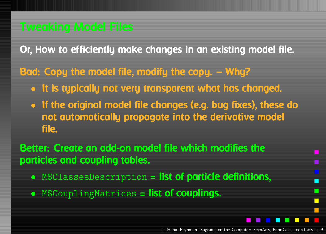
Tweaking Model Files
Or, How to efficiently make changes in an existing model file.
Bad: Copy the model file, modify the copy. — Why?
• It is typically not very transparent what has changed.
• If the original model file changes (e.g. bug fixes), these donot automatically propagate into the derivative modelfile.
Better: Create an add-on model file which modifies theparticles and coupling tables.
• M$ClassesDescription = list of particle definitions,
• M$CouplingMatrices = list of couplings.
T. Hahn, Feynman Diagrams on the Computer: FeynArts, FormCalc, LoopTools – p.9

Tweaking Model Files
Example: Introduce enhancement factors for the b–b̄–h0 andb–b̄–H0 Yukawa couplings in the MSSM.
EnhCoup[(lhs:C[F[4,{g_,_}], -F[4,_], S[h:1|2]]) == rhs_] :=
lhs == Hff[h,g] rhs
EnhCoup[other_] = other
M$CouplingMatrices = EnhCoup/@ M$CouplingMatrices
T. Hahn, Feynman Diagrams on the Computer: FeynArts, FormCalc, LoopTools – p.10

Linear Combinations of Fields
FeynArts can automatically linear-combine fields, i.e. onecan specify the couplings in terms of gauge rather than masseigenstates. For example:
M$ClassesDescription = { ...,
F[11] = {...,
Indices -> {Index[Neutralino]},
Mixture -> ZNeu[Index[Neutralino],1] F[111] +
ZNeu[Index[Neutralino],2] F[112] +
ZNeu[Index[Neutralino],3] F[113] +
ZNeu[Index[Neutralino],4] F[114]} }
Since F[111]. . . F[114] are not listed in M$CouplingMatrices,they drop out of the model completely.
T. Hahn, Feynman Diagrams on the Computer: FeynArts, FormCalc, LoopTools – p.11
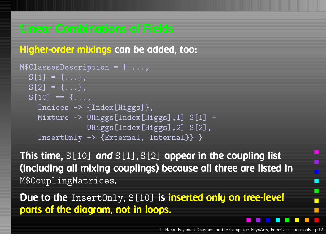
Linear Combinations of Fields
Higher-order mixings can be added, too:
M$ClassesDescription = { ...,
S[1] = {...},
S[2] = {...},
S[10] == {...,
Indices -> {Index[Higgs]},
Mixture -> UHiggs[Index[Higgs],1] S[1] +
UHiggs[Index[Higgs],2] S[2],
InsertOnly -> {External, Internal}} }
This time, S[10] and S[1], S[2] appear in the coupling list(including all mixing couplings) because all three are listed inM$CouplingMatrices.
Due to the InsertOnly, S[10] is inserted only on tree-levelparts of the diagram, not in loops.
T. Hahn, Feynman Diagrams on the Computer: FeynArts, FormCalc, LoopTools – p.12

Enhanced Diagram Selection
FeynArts has easier way to pick wave-function corrections:CreateTopologies[ ...
ExcludeTopologies -> WFCorrections[1|3] ]
Select only those where the in- and out-fields of theself-energy are not the same:
DiagramSelect[ ...,
UnsameQ@@ WFCorrectionFields[##] & ]
✔
H
W
h0
Gνl
el
✘
H
W
h0
Wνl
el
T. Hahn, Feynman Diagrams on the Computer: FeynArts, FormCalc, LoopTools – p.13

Enhanced Diagram Selection
The new FeynArts function FermionRouting can be used toselect diagrams according to their fermion structure, e.g.
DiagramSelect[...,
FermionRouting[##] === {1,3, 2,4} & ]
selects only diagrams where external legs 1–3 and 2–4 areconnected through fermion lines.
✔
1
2
3
4 ✘
1
2
3
4
More Functions: DiagramGrouping, DiagramMap, DiagramComplement.More Filters: Vertices, FieldPoints, FeynAmpCases, FieldMatchQ,FieldMemberQ, FieldPointMatchQ, FieldPointMemberQ.
T. Hahn, Feynman Diagrams on the Computer: FeynArts, FormCalc, LoopTools – p.14

Programming Diagram Filters
Or, What if FeynArts’ selection functions are not enough.
Observe the structure of inserted topologies:TopologyList[__][t1, t2, ...]
ti: Topology[_][__] -> Insertions[Generic][g1, g2, ...]
gi: Graph[__][__] -> Insertion[Classes][c1, c2, ...]
ci: Graph[__][__] -> Insertion[Particles][p1, p2, ...]
Example: Select the diagrams with only fermion loops.FermionLoop[t:TopologyList[___][__]] := FermionLoop/@ t
FermionLoop[(top:Topology[_][__]) -> ins:Insertions[Generic][__]] :=
top -> TestLoops[top]/@ ins
TestLoops[top_][gi_ -> ci_] := (gi -> ci) /;
MatchQ[Cases[top /. List@@ gi,
Propagator[Loop[_]][v1_, v2_, field_] -> field]], F..]
TestLoops[_][_] := Sequence[]
T. Hahn, Feynman Diagrams on the Computer: FeynArts, FormCalc, LoopTools – p.15
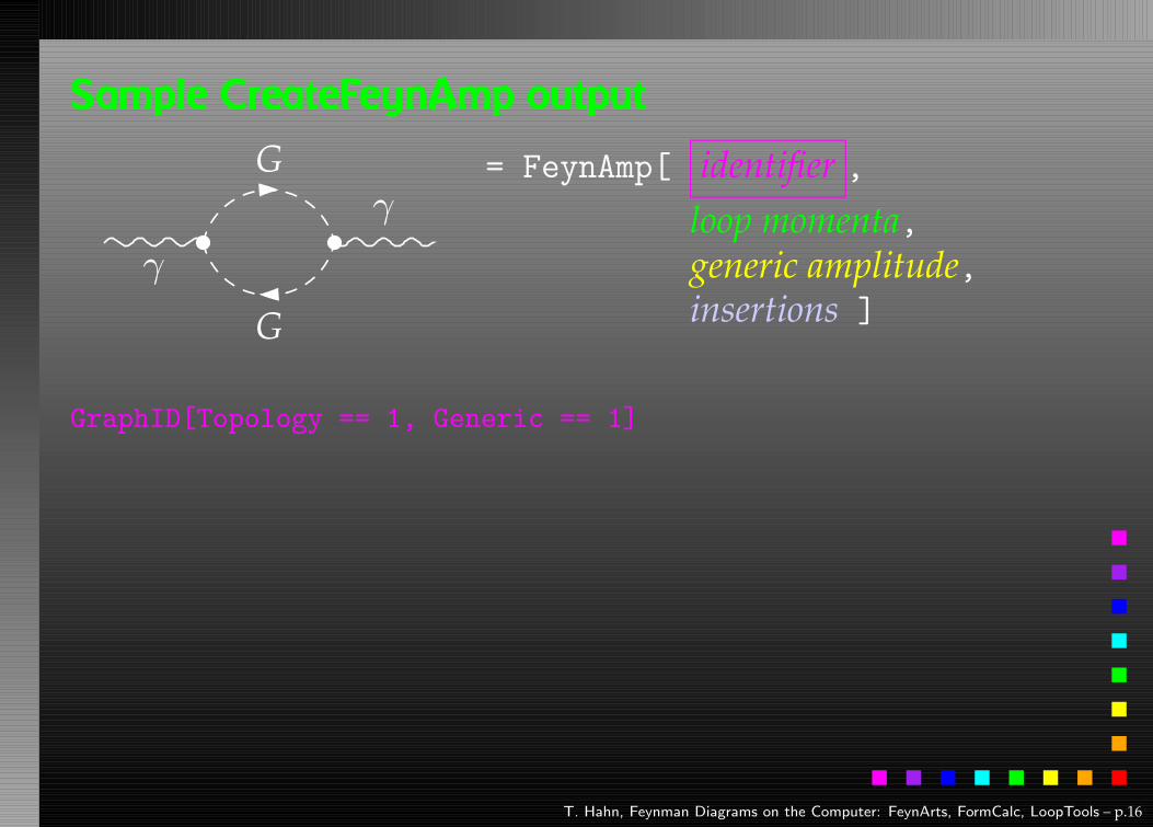
Sample CreateFeynAmp output
γ
γ
G
G = FeynAmp[ identifier ,loop momenta,generic amplitude,insertions ]
GraphID[Topology == 1, Generic == 1]
T. Hahn, Feynman Diagrams on the Computer: FeynArts, FormCalc, LoopTools – p.16

Sample CreateFeynAmp output
γ
γ
G
G = FeynAmp[ identifier,loop momenta ,
generic amplitude,insertions ]
Integral[q1]
T. Hahn, Feynman Diagrams on the Computer: FeynArts, FormCalc, LoopTools – p.17

Sample CreateFeynAmp output
γ
γ
G
G = FeynAmp[ identifier,loop momenta,generic amplitude ,
insertions ]
I
32 Pi4RelativeCF .........................................prefactor
FeynAmpDenominator[1
q12 - Mass[S[Gen3]]2,
1
(-p1 + q1)2 - Mass[S[Gen4]]2] .................loop denominators
(p1 - 2 q1)[Lor1] (-p1 + 2 q1)[Lor2] ........ kin. coupling structure
ep[V[1], p1, Lor1] ep*[V[1], k1, Lor2] ...........polarization vectors
G(0)SSV[(Mom[1] - Mom[2])[KI1[3]]]
G(0)SSV[(Mom[1] - Mom[2])[KI1[3]]] ...................coupling constants
T. Hahn, Feynman Diagrams on the Computer: FeynArts, FormCalc, LoopTools – p.18
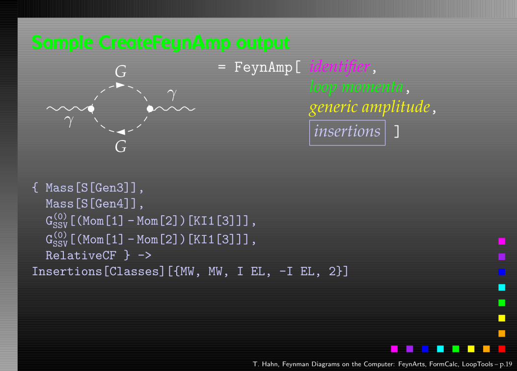
Sample CreateFeynAmp output
γ
γ
G
G = FeynAmp[ identifier,loop momenta,generic amplitude,insertions ]
{ Mass[S[Gen3]],
Mass[S[Gen4]],
G(0)SSV[(Mom[1] - Mom[2])[KI1[3]]],
G(0)SSV[(Mom[1] - Mom[2])[KI1[3]]],
RelativeCF } ->
Insertions[Classes][{MW, MW, I EL, -I EL, 2}]
T. Hahn, Feynman Diagrams on the Computer: FeynArts, FormCalc, LoopTools – p.19

Algebraic Simplification
The amplitudes of CreateFeynAmp are in no good shape fordirect numerical evaluation.
A number of steps have to be done analytically:
• contract indices as far as possible,
• evaluate fermion traces,
• perform the tensor reduction,
• add local terms arising from D·(divergent integral)(dim reg + dim red),
• simplify open fermion chains,
• simplify and compute the square of SU(N) structures,
• “compactify” the results as much as possible.T. Hahn, Feynman Diagrams on the Computer: FeynArts, FormCalc, LoopTools – p.20
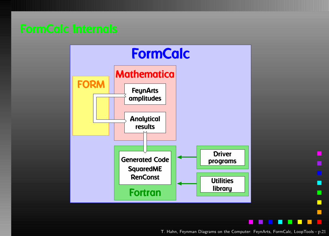
FormCalc Internals
FormCalcMathematica
FORMFeynArts
amplitudes
Analyticalresults
Fortran
Generated CodeSquaredMERenConst
Driverprograms
Utilitieslibrary
T. Hahn, Feynman Diagrams on the Computer: FeynArts, FormCalc, LoopTools – p.21

FormCalc Output
A typical term in the output looks like
C0i[cc12, MW2, MW2, S, MW2, MZ2, MW2] *
( -4 Alfa2 MW2 CW2/SW2 S AbbSum16 +
32 Alfa2 CW2/SW2 S2 AbbSum28 +
4 Alfa2 CW2/SW2 S2 AbbSum30 -
8 Alfa2 CW2/SW2 S2 AbbSum7 +
Alfa2 CW2/SW2 S (T - U) Abb1 +
8 Alfa2 CW2/SW2 S (T - U) AbbSum29 )
= loop integral = kinematical variables
= constants = automatically introduced abbreviations
T. Hahn, Feynman Diagrams on the Computer: FeynArts, FormCalc, LoopTools – p.22

Abbreviations
Outright factorization is usually out of question.Abbreviations are necessary to reduce size of expressions.
AbbSum29 = Abb2 + Abb22 + Abb23 + Abb3
Abb22 = Pair1 Pair3 Pair6
Pair3 = Pair[e[3], k[1]]
The full expression corresponding to AbbSum29 isPair[e[1], e[2]] Pair[e[3], k[1]] Pair[e[4], k[1]] +
Pair[e[1], e[2]] Pair[e[3], k[2]] Pair[e[4], k[1]] +
Pair[e[1], e[2]] Pair[e[3], k[1]] Pair[e[4], k[2]] +
Pair[e[1], e[2]] Pair[e[3], k[2]] Pair[e[4], k[2]]
T. Hahn, Feynman Diagrams on the Computer: FeynArts, FormCalc, LoopTools – p.23
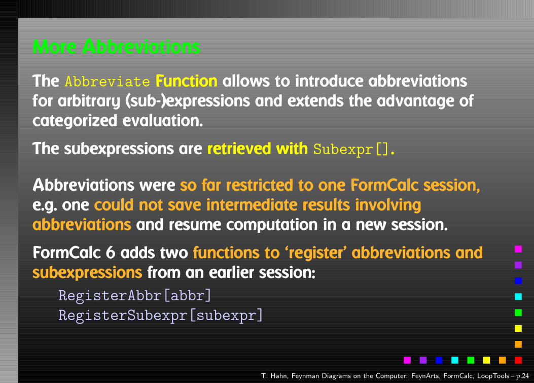
More Abbreviations
The Abbreviate Function allows to introduce abbreviationsfor arbitrary (sub-)expressions and extends the advantage ofcategorized evaluation.
The subexpressions are retrieved with Subexpr[].
Abbreviations were so far restricted to one FormCalc session,e.g. one could not save intermediate results involvingabbreviations and resume computation in a new session.
FormCalc 6 adds two functions to ‘register’ abbreviations andsubexpressions from an earlier session:
RegisterAbbr[abbr]
RegisterSubexpr[subexpr]
T. Hahn, Feynman Diagrams on the Computer: FeynArts, FormCalc, LoopTools – p.24

Categories of Abbreviations
• Abbreviations are recursively defined in several levels.
• When generating Fortran code, FormCalc introducesanother set of abbreviations for the loop integrals.
In general, the abbreviations are thus costly in CPU time.It is key to a decent performance that the abbreviations areseparated into different Categories:
• Abbreviations that depend on the helicities,
• Abbreviations that depend on angular variables,
• Abbreviations that depend only on√
s.
Correct execution of the categories guarantees that almost noredundant evaluations are made and makes the generatedcode essentially as fast as hand-tuned code.
T. Hahn, Feynman Diagrams on the Computer: FeynArts, FormCalc, LoopTools – p.25

External Fermion Lines
An amplitude containing external fermions has the form
M =nF
∑i=1
ci Fi where Fi = (Product of) 〈u|Γi |v〉 .
nF = number of fermionic structures.
Textbook procedure: Trace Technique
|M|2 =nF
∑i, j=1
c∗i c j F∗i Fj
where F∗i Fj = 〈v| Γ̄i |u〉 〈u|Γ j |v〉 = Tr(Γ̄i |u〉〈u| Γ j |v〉〈v|
).
T. Hahn, Feynman Diagrams on the Computer: FeynArts, FormCalc, LoopTools – p.26

Problems with the Trace Technique
PRO: Trace technique is independent of any representation.
CON: For nF Fi’s there are n2F F∗i Fj’s.
Things get worse the more vectors are in the game:multi-particle final states, polarization effects . . .Essentially nF ∼ (# of vectors)! because allcombinations of vectors can appear in the Γi.
Solution: Use Weyl–van der Waerden spinor formalism tocompute the Fi’s directly.
T. Hahn, Feynman Diagrams on the Computer: FeynArts, FormCalc, LoopTools – p.27

Sigma Chains
Define Sigma matrices and 2-dim. Spinors as
σµ = (1l,−~σ) ,
σµ = (1l,+~σ) ,
〈u|4d ≡(〈u+|2d , 〈u−|2d
),
|v〉4d ≡(|v−〉2d
|v+〉2d
).
Using the chiral representation it is easy to show thatevery chiral 4-dim. Dirac chain can be converted to asingle 2-dim. sigma chain:
〈u|ω−γµγν · · · |v〉 = 〈u−|σµσν · · · |v±〉 ,〈u|ω+γµγν · · · |v〉 = 〈u+|σµσν · · · |v∓〉 .
T. Hahn, Feynman Diagrams on the Computer: FeynArts, FormCalc, LoopTools – p.28
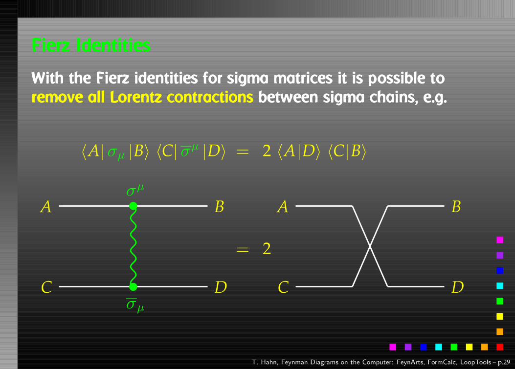
Fierz Identities
With the Fierz identities for sigma matrices it is possible toremove all Lorentz contractions between sigma chains, e.g.
〈A|σµ |B〉 〈C|σµ |D〉 = 2 〈A|D〉 〈C|B〉
A B
C D
σµ
σµ
= 2
A
D
B
C
T. Hahn, Feynman Diagrams on the Computer: FeynArts, FormCalc, LoopTools – p.29
Implementation
• Objects (arrays): |u±〉 ∼(
u1u2
), (σ · k) ∼
(a bc d
)
• Operations (functions):
〈u|v〉 ∼ (u1 u2) ·(
v1v2
)SxS
(( )σ · k) |v〉 ∼(
a bc d
)·(
v1v2
)VxS, BxS
Sufficient to compute any sigma chain:
〈u|σµσνσρ |v〉 kµ1 kν2 kρ3 = SxS(u, VxS(k1, BxS(k2, VxS(k3, v))))
T. Hahn, Feynman Diagrams on the Computer: FeynArts, FormCalc, LoopTools – p.30

More Freebies
• Polarization does not ‘cost’ extra= Get spin physics for free.
• Better numerical stability because components of kµ arearranged as ‘small’ and ‘large’ matrix entries, viz.
σµkµ =
(k0 + k3 k1 − ik2
k1 + ik2 k0 − k3↓
)
Large cancellations of the form√
k2 + m2 −√
k2 whenm� k are avoided: better precision for mass effects.
T. Hahn, Feynman Diagrams on the Computer: FeynArts, FormCalc, LoopTools – p.31

Dirac Chains in 4D
As numerical calculations are done mostly using Weyl-spinorchains, there has been a paradigm shift for Dirac chains tomake them better suited for analytical purposes, e.g. theextraction of Wilson coefficients.
• Already in Version 5, Fierz methods have beenimplemented for Dirac chains, thus allowing the user toforce the fermion chains into almost any desired order.
• Version 6 further adds the Colour method to theFermionOrder option of CalcFeynAmp, which brings thespinors into the same order as the external colour indices.
• Also new in Version 6: completely antisymmetrizedDirac chains, i.e. DiracChain[−1, µ, ν] = σµν .
T. Hahn, Feynman Diagrams on the Computer: FeynArts, FormCalc, LoopTools – p.32

Alternate Link between FORM and Mathematica
FORM is able to handle very large expressions. To produce(pre-)simplified expressions, however, terms have to bewrapped in functions, to avoid immediate expansion:
a*(b + c) → a*b + a*c
a*f(b + c) → a*f(b + c)
The number of terms in a function is rather limited in FORM:on 32-bit systems to 32767.
Dilemma: FormCalc gets more sophisticated in pre-simplifyingamplitudes while users want to compute larger amplitudes.Thus, recently many ‘overflow’ messages from FORM.
Solution: Send pre-simplified generic amplitude via externalchannel to Mathematica for introducing abbreviations.Significant reduction in size of intermediate expressions.Tentukov, Vermaseren 2006
T. Hahn, Feynman Diagrams on the Computer: FeynArts, FormCalc, LoopTools – p.33
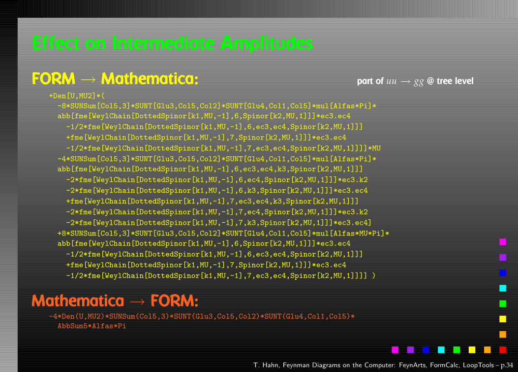
Effect on Intermediate Amplitudes
FORM → Mathematica: part of uu→ gg @ tree level+Den[U,MU2]*(
-8*SUNSum[Col5,3]*SUNT[Glu3,Col5,Col2]*SUNT[Glu4,Col1,Col5]*mul[Alfas*Pi]*
abb[fme[WeylChain[DottedSpinor[k1,MU,-1],6,Spinor[k2,MU,1]]]*ec3.ec4
-1/2*fme[WeylChain[DottedSpinor[k1,MU,-1],6,ec3,ec4,Spinor[k2,MU,1]]]
+fme[WeylChain[DottedSpinor[k1,MU,-1],7,Spinor[k2,MU,1]]]*ec3.ec4
-1/2*fme[WeylChain[DottedSpinor[k1,MU,-1],7,ec3,ec4,Spinor[k2,MU,1]]]]*MU
-4*SUNSum[Col5,3]*SUNT[Glu3,Col5,Col2]*SUNT[Glu4,Col1,Col5]*mul[Alfas*Pi]*
abb[fme[WeylChain[DottedSpinor[k1,MU,-1],6,ec3,ec4,k3,Spinor[k2,MU,1]]]
-2*fme[WeylChain[DottedSpinor[k1,MU,-1],6,ec4,Spinor[k2,MU,1]]]*ec3.k2
-2*fme[WeylChain[DottedSpinor[k1,MU,-1],6,k3,Spinor[k2,MU,1]]]*ec3.ec4
+fme[WeylChain[DottedSpinor[k1,MU,-1],7,ec3,ec4,k3,Spinor[k2,MU,1]]]
-2*fme[WeylChain[DottedSpinor[k1,MU,-1],7,ec4,Spinor[k2,MU,1]]]*ec3.k2
-2*fme[WeylChain[DottedSpinor[k1,MU,-1],7,k3,Spinor[k2,MU,1]]]*ec3.ec4]
+8*SUNSum[Col5,3]*SUNT[Glu3,Col5,Col2]*SUNT[Glu4,Col1,Col5]*mul[Alfas*MU*Pi]*
abb[fme[WeylChain[DottedSpinor[k1,MU,-1],6,Spinor[k2,MU,1]]]*ec3.ec4
-1/2*fme[WeylChain[DottedSpinor[k1,MU,-1],6,ec3,ec4,Spinor[k2,MU,1]]]
+fme[WeylChain[DottedSpinor[k1,MU,-1],7,Spinor[k2,MU,1]]]*ec3.ec4
-1/2*fme[WeylChain[DottedSpinor[k1,MU,-1],7,ec3,ec4,Spinor[k2,MU,1]]]] )
Mathematica → FORM:-4*Den(U,MU2)*SUNSum(Col5,3)*SUNT(Glu3,Col5,Col2)*SUNT(Glu4,Col1,Col5)*
AbbSum5*Alfas*Pi
T. Hahn, Feynman Diagrams on the Computer: FeynArts, FormCalc, LoopTools – p.34

Numerical Evaluation in Fortran 77
user-level code included in FormCalc
generated code, “black box”
Cross-sections, Decay rates, Asymmetries . . .
SquaredME.Fmaster subroutine
abbr0_s.F
abbr0_angle.F...
abbreviations(invoked onlywhen necessary)
born.F
self.F...
form factors
xsection.Fdriver program
run.Fparameters for this run
process.hprocess definition
main.F
CPU-time (rough)
compute abbrtree}
5 %
compute abbr1-loop}
95 %
computeMtree}
.1 %
computeM1-loop}
.1 %
T. Hahn, Feynman Diagrams on the Computer: FeynArts, FormCalc, LoopTools – p.35
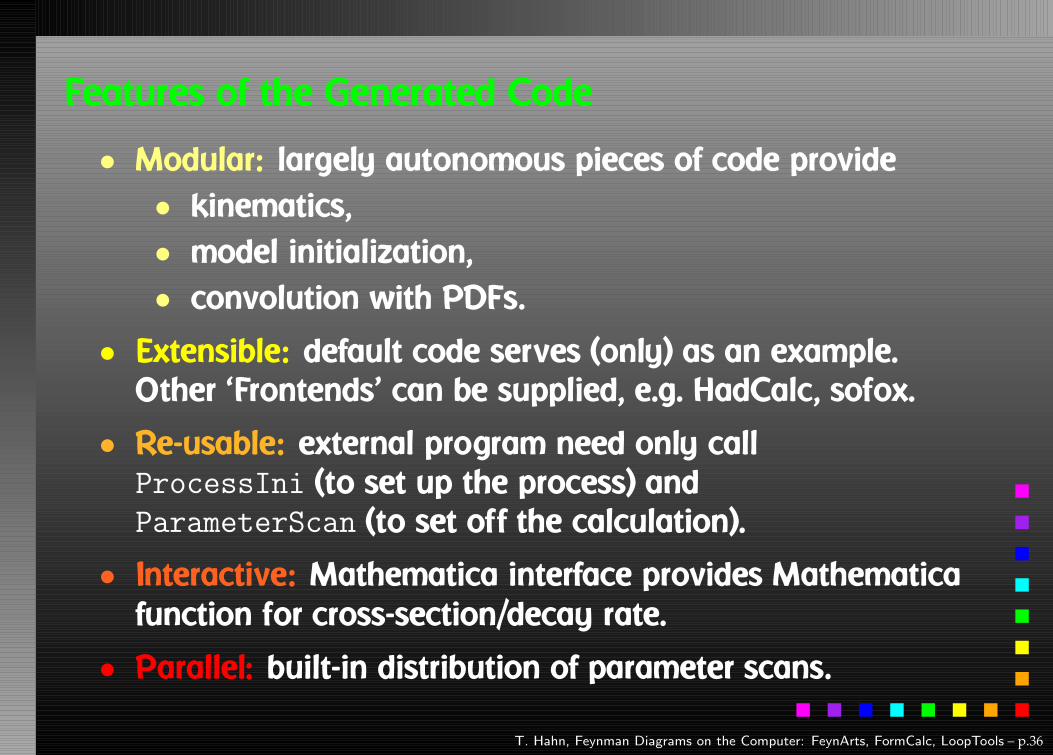
Features of the Generated Code
• Modular: largely autonomous pieces of code provide• kinematics,• model initialization,• convolution with PDFs.
• Extensible: default code serves (only) as an example.Other ‘Frontends’ can be supplied, e.g. HadCalc, sofox.
• Re-usable: external program need only callProcessIni (to set up the process) andParameterScan (to set off the calculation).
• Interactive: Mathematica interface provides Mathematicafunction for cross-section/decay rate.
• Parallel: built-in distribution of parameter scans.
T. Hahn, Feynman Diagrams on the Computer: FeynArts, FormCalc, LoopTools – p.36

Choice of Language
Mentioning Fortran 77 as the programming language in manycircles draws a “Not that dinosaur again” response.But consider:
• Fortran was designed for ‘number crunching,’ i.e. efficientevaluation of large formulas.
• Good and free compilers are available.
• Fortran is still widely used in theoretical physics.
• The code is generated, so largely ‘invisible’ for the user.
• Linking Fortran 77 to C/C++ is pretty straightforward(particularly inside gcc), so is in some sense a ‘smallestcommon denominator.’
T. Hahn, Feynman Diagrams on the Computer: FeynArts, FormCalc, LoopTools – p.37
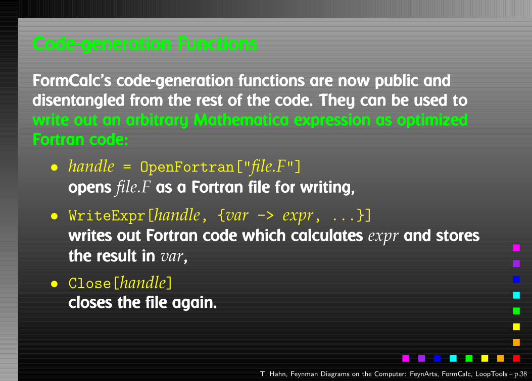
Code-generation Functions
FormCalc’s code-generation functions are now public anddisentangled from the rest of the code. They can be used towrite out an arbitrary Mathematica expression as optimizedFortran code:
• handle = OpenFortran["file.F"]opens file.F as a Fortran file for writing,
• WriteExpr[handle, {var -> expr, ...}]
writes out Fortran code which calculates expr and storesthe result in var,
• Close[handle]closes the file again.
T. Hahn, Feynman Diagrams on the Computer: FeynArts, FormCalc, LoopTools – p.38

Code generation
• Expressions too large for Fortran are split into parts, as in
var = part1
var = var + part2
...
• High level of optimization, e.g. common subexpressionsare pulled out and computed in temporary variables.
• Many ancillary functions, e.g.PrepareExpr, OnePassOrder, SplitSums,$SymbolPrefix, CommonDecl, SubroutineDecl,etc.
make code generation versatile and highly automatable.Resulting code needs few or no changes by hand.
T. Hahn, Feynman Diagrams on the Computer: FeynArts, FormCalc, LoopTools – p.39

Not the Cross-Section
Or, How to get things the Standard Setup won’t give you.
Example: extract the Wilson coefficients for b→ sγ .tops = CreateTopologies[1, 1 -> 2]
ins = InsertFields[tops, F[4,{3}] -> {F[4,{2}], V[1]}]
vert = CalcFeynAmp[CreateFeynAmp[ins], FermionChains -> Chiral]
mat[p_Plus] := mat/@ p
mat[r_. DiracChain[s2_Spinor, om_, mu_, s1:Spinor[p1_, m1_, _]]] :=
I/(2 m1) mat[r DiracChain[sigmunu[om]]] +
2/m1 r Pair[mu, p1] DiracChain[s2, om, s1]
mat[r_. DiracChain[sigmunu[om_]], SUNT[Col1, Col2]] :=
r O7[om]/(EL MB/(16 Pi^2))
mat[r_. DiracChain[sigmunu[om_]], SUNT[Glu1, Col2, Col1]] :=
r O8[om]/(GS MB/(16 Pi^2))
coeff = Plus@@ vert //. abbr /. Mat -> mat
c7 = Coefficient[coeff, O7[6]]
c8 = Coefficient[coeff, O8[6]]
T. Hahn, Feynman Diagrams on the Computer: FeynArts, FormCalc, LoopTools – p.40

Not the Cross-Section
Using FormCalc’s output functions it is also prettystraightforward to generate your own Fortran code:
file = OpenFortran["bsgamma.F"]
WriteString[file,
SubroutineDecl["bsgamma(C7,C8)"] <>
"\tdouble complex C7, C8\n" <>
"#include \"looptools.h\"\n"]
WriteExpr[file, {C7 -> c7, C8 -> c8}]
WriteString[file, "\tend\n"]
Close[file]
T. Hahn, Feynman Diagrams on the Computer: FeynArts, FormCalc, LoopTools – p.41
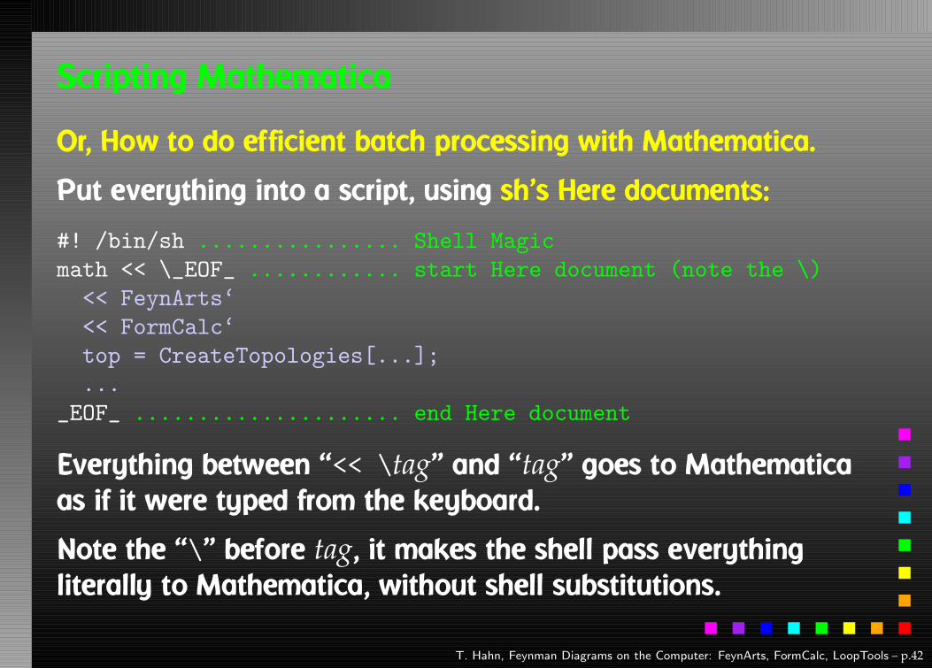
Scripting Mathematica
Or, How to do efficient batch processing with Mathematica.
Put everything into a script, using sh’s Here documents:
#! /bin/sh ................ Shell Magic
math << \_EOF_ ............ start Here document (note the \)
<< FeynArts‘
<< FormCalc‘
top = CreateTopologies[...];
...
_EOF_ ..................... end Here document
Everything between “<< \tag” and “tag” goes to Mathematicaas if it were typed from the keyboard.
Note the “\” before tag, it makes the shell pass everythingliterally to Mathematica, without shell substitutions.
T. Hahn, Feynman Diagrams on the Computer: FeynArts, FormCalc, LoopTools – p.42
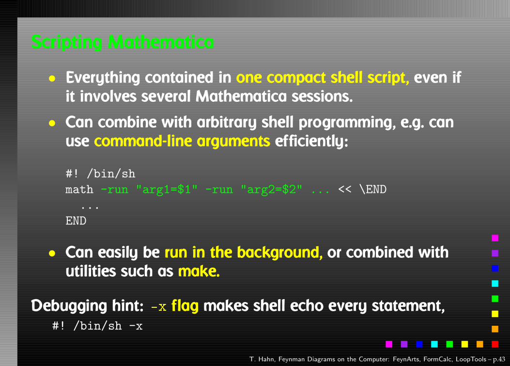
Scripting Mathematica
• Everything contained in one compact shell script, even ifit involves several Mathematica sessions.
• Can combine with arbitrary shell programming, e.g. canuse command-line arguments efficiently:
#! /bin/sh
math -run "arg1=$1" -run "arg2=$2" ... << \END
...
END
• Can easily be run in the background, or combined withutilities such as make.
Debugging hint: � � flag makes shell echo every statement,#! /bin/sh -x
T. Hahn, Feynman Diagrams on the Computer: FeynArts, FormCalc, LoopTools – p.43
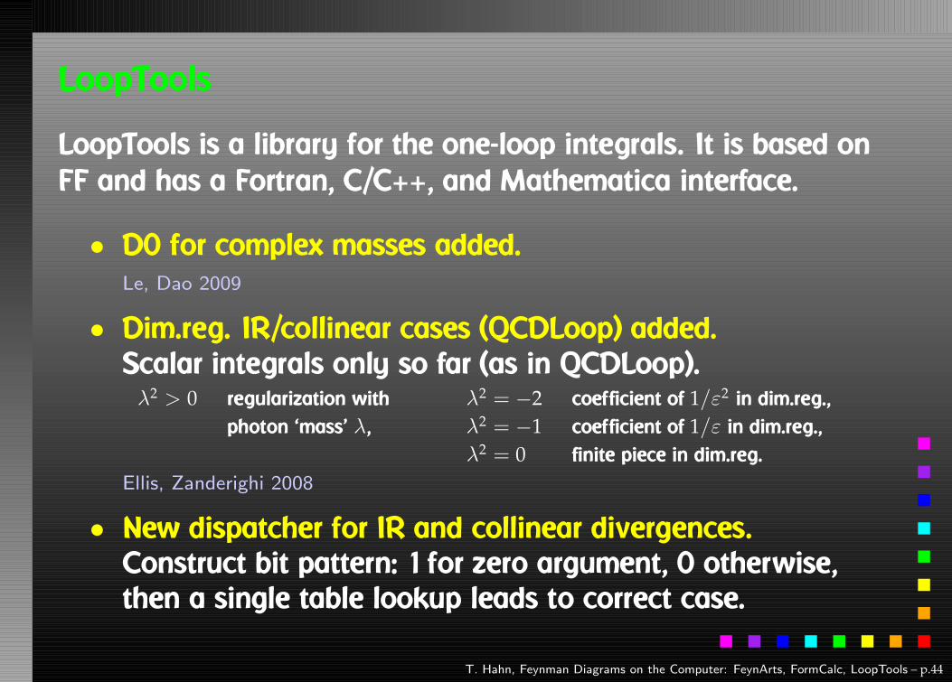
LoopTools
LoopTools is a library for the one-loop integrals. It is based onFF and has a Fortran, C/C++, and Mathematica interface.
• D0 for complex masses added.Le, Dao 2009
• Dim.reg. IR/collinear cases (QCDLoop) added.Scalar integrals only so far (as in QCDLoop).λ2 > 0 regularization with λ2 = −2 coefficient of 1/ε2 in dim.reg.,
photon ‘mass’ λ, λ2 = −1 coefficient of 1/ε in dim.reg.,λ2 = 0 finite piece in dim.reg.
Ellis, Zanderighi 2008
• New dispatcher for IR and collinear divergences.Construct bit pattern: 1 for zero argument, 0 otherwise,then a single table lookup leads to correct case.
T. Hahn, Feynman Diagrams on the Computer: FeynArts, FormCalc, LoopTools – p.44

LoopTools Environment Variables
Most LoopTools parameters can be set from the outsidethrough environment variables:LTCMPBITS # of bits compared in cache lookupsLTVERSION bit mask for alternate versionsLTMAXDEV maximum allowed relative deviation in comparing to alternate versionsLTDEBUG bit mask for debuggingLTRANGE range of integrals to print out in debug modeLTWARN number of digits lost before warningLTERR number of digits lost before errorLTDELTA ‘divergence’ ∆LTMUDIM renormalization scale µ2
LTLAMBDA IR regulator parameter λ2
LTMINMASS threshold m2min below which particles are considered ‘massless’
E.g. check finiteness without re-compilation by modifyingLTMUDIM, LTLAMBDA.
T. Hahn, Feynman Diagrams on the Computer: FeynArts, FormCalc, LoopTools – p.45
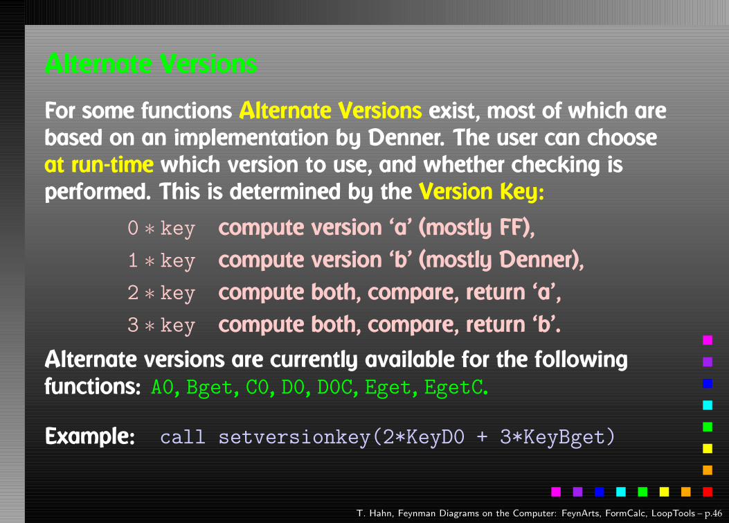
Alternate Versions
For some functions Alternate Versions exist, most of which arebased on an implementation by Denner. The user can chooseat run-time which version to use, and whether checking isperformed. This is determined by the Version Key:
0 ∗ key compute version ‘a’ (mostly FF),1 ∗ key compute version ‘b’ (mostly Denner),2 ∗ key compute both, compare, return ‘a’,3 ∗ key compute both, compare, return ‘b’.
Alternate versions are currently available for the followingfunctions: A0, Bget, C0, D0, D0C, Eget, EgetC.
Example: call setversionkey(2*KeyD0 + 3*KeyBget)
T. Hahn, Feynman Diagrams on the Computer: FeynArts, FormCalc, LoopTools – p.46

Command-line Interface
The Command-lineInterface is useful inparticular for testingand debugging.
It lists the N-pointscalar and tensorcoefficientscorresponding to thenumber of arguments,i.e. 3 arguments = B,6 arguments = C, etc.
> lt 250000 6464.16 8315.38
====================================================
FF 2.0, a package to evaluate one-loop integrals
written by G. J. van Oldenborgh, NIKHEF-H, Amsterdam
====================================================
for the algorithms used see preprint NIKHEF-H 89/17,
’New Algorithms for One-loop Integrals’, by G.J. van
Oldenborgh and J.A.M. Vermaseren, published in
Zeitschrift fuer Physik C46(1990)425.
====================================================
p = 250000.000000000
m1 = 6464.16000000000
m2 = 8315.38000000000
bb0 = (-10.1569090105893,2.95011861955466)
bb1 = (5.07382021909957,-1.46413667259555)
bb00 = (165409.773493414,-54197.2752510472)
bb11 = (-3.31323987482202,0.943436559119877)
bb001 = (-81984.2510317697,26897.9754657431)
bb111 = (2.43370306005361,-0.683409066031936)
dbb0 = (-4.868613391538015E-006,7.903840552878544E-007)
dbb1 = (2.434818091584023E-006,-4.359562268294025E-007)
dbb00 = (0.880290172138776,-0.260350056737834)
dbb11 = (-1.624235905363170E-006,4.122913473051599E-007)
====================================================
total number of errors and warnings
===================================
fferr: no errors
T. Hahn, Feynman Diagrams on the Computer: FeynArts, FormCalc, LoopTools – p.47

CutTools
Tensor loop integrals have in FormCalc so far been treated byPassarino–Veltman reduction only, e.g.
qµqνD0D1
= gµν B00(p2,m21,m
22) + pµpν B11(p2,m2
1,m22)
where B00 and B11 are provided by LoopTools.
CutTools implements the cutting-technique-inspired OPP(Ossola, Papadopoulos, Pittau) method. It needs thenumerator as a function of q which it can sample:
Bcut(2, num, p,m21,m
22)
where num = qµqν .
Independent way of checking LoopTools results.Performance?
T. Hahn, Feynman Diagrams on the Computer: FeynArts, FormCalc, LoopTools – p.48

A Final Look
Using FeynArts, FormCalc, and LoopTools is a lot like drivinga car:
• You have to decide where to go (this is often the hardestdecision).
• You have to turn the ignition key, work gas and brakes,and steer.
• But you don’t have to know, say, which valve has toopen at which time to keep the motor running.
• On the other hand, you can only go where there areroads. You can’t climb a mountain with your car.
feynarts.de
T. Hahn, Feynman Diagrams on the Computer: FeynArts, FormCalc, LoopTools – p.49
Related Documents