FEW THEORETICAL REMARKS ON THE DYNAMICAL CONTROL …

Lecture 12: Example of home work on an America Cup

FEW THEORETICAL REMARKS ON THE DYNAMICAL CONTROL OFRACING SAILING BOATS WITH FOILS

PHILIPPE DESTUYNDER∗ AND CAROLINE FABRE∗∗

* Département d’ingénierie mathématique, laboratoire M2NConservatoire National des Arts et Métiers292, rue saint Martin, 75003 Paris France

[email protected]** Laboratoire de mathématiques d’Orsay, UMR 8628

Univ Paris-Sud, CNRS, Université Paris-SaclayOrsay 91405 France

[email protected]

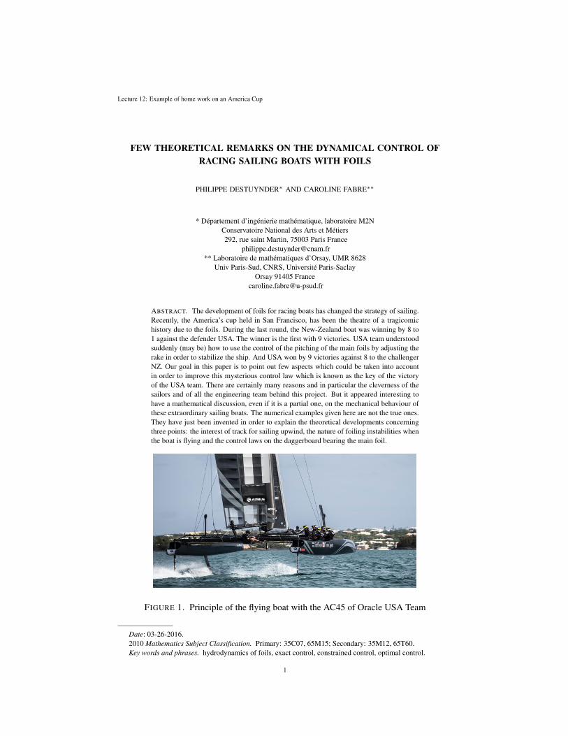
ABSTRACT. The development of foils for racing boats has changed the strategy of sailing.Recently, the America’s cup held in San Francisco, has been the theatre of a tragicomichistory due to the foils. During the last round, the New-Zealand boat was winning by 8 to1 against the defender USA. The winner is the first with 9 victories. USA team understoodsuddenly (may be) how to use the control of the pitching of the main foils by adjusting therake in order to stabilize the ship. And USA won by 9 victories against 8 to the challengerNZ. Our goal in this paper is to point out few aspects which could be taken into accountin order to improve this mysterious control law which is known as the key of the victoryof the USA team. There are certainly many reasons and in particular the cleverness of thesailors and of all the engineering team behind this project. But it appeared interesting tohave a mathematical discussion, even if it is a partial one, on the mechanical behaviour ofthese extraordinary sailing boats. The numerical examples given here are not the true ones.They have just been invented in order to explain the theoretical developments concerningthree points: the interest of track for sailing upwind, the nature of foiling instabilities whenthe boat is flying and the control laws on the daggerboard bearing the main foil.

FIGURE 1. Principle of the flying boat with the AC45 of Oracle USA Team

Date: 03-26-2016.2010 Mathematics Subject Classification. Primary: 35C07, 65M15; Secondary: 35M12, 65T60.Key words and phrases. hydrodynamics of foils, exact control, constrained control, optimal control.

1

2 PH. D.

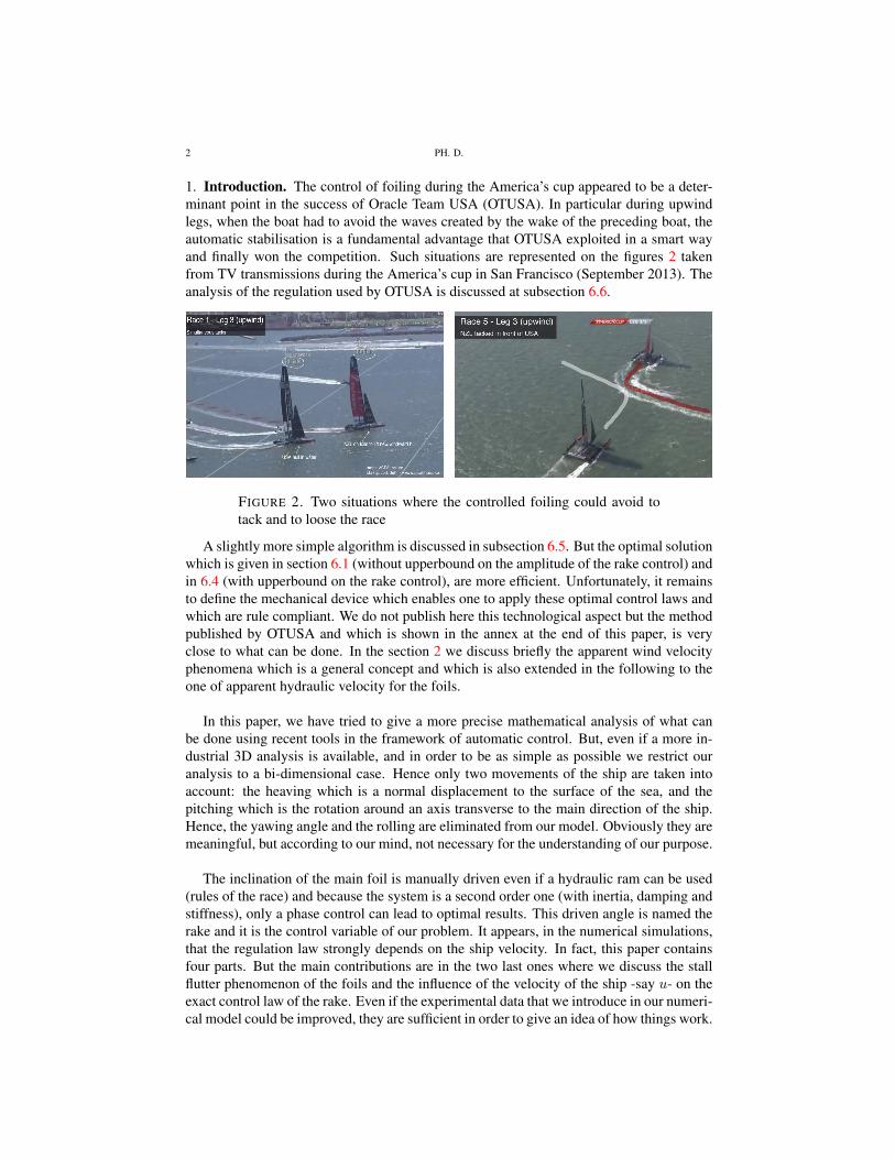
1. Introduction. The control of foiling during the America’s cup appeared to be a deter-minant point in the success of Oracle Team USA (OTUSA). In particular during upwindlegs, when the boat had to avoid the waves created by the wake of the preceding boat, theautomatic stabilisation is a fundamental advantage that OTUSA exploited in a smart wayand finally won the competition. Such situations are represented on the figures 2 takenfrom TV transmissions during the America’s cup in San Francisco (September 2013). Theanalysis of the regulation used by OTUSA is discussed at subsection 6.6.

FIGURE 2. Two situations where the controlled foiling could avoid totack and to loose the race

A slightly more simple algorithm is discussed in subsection 6.5. But the optimal solutionwhich is given in section 6.1 (without upperbound on the amplitude of the rake control) andin 6.4 (with upperbound on the rake control), are more efficient. Unfortunately, it remainsto define the mechanical device which enables one to apply these optimal control laws andwhich are rule compliant. We do not publish here this technological aspect but the methodpublished by OTUSA and which is shown in the annex at the end of this paper, is veryclose to what can be done. In the section 2 we discuss briefly the apparent wind velocityphenomena which is a general concept and which is also extended in the following to theone of apparent hydraulic velocity for the foils.

In this paper, we have tried to give a more precise mathematical analysis of what canbe done using recent tools in the framework of automatic control. But, even if a more in-dustrial 3D analysis is available, and in order to be as simple as possible we restrict ouranalysis to a bi-dimensional case. Hence only two movements of the ship are taken intoaccount: the heaving which is a normal displacement to the surface of the sea, and thepitching which is the rotation around an axis transverse to the main direction of the ship.Hence, the yawing angle and the rolling are eliminated from our model. Obviously they aremeaningful, but according to our mind, not necessary for the understanding of our purpose.

The inclination of the main foil is manually driven even if a hydraulic ram can be used(rules of the race) and because the system is a second order one (with inertia, damping andstiffness), only a phase control can lead to optimal results. This driven angle is named therake and it is the control variable of our problem. It appears, in the numerical simulations,that the regulation law strongly depends on the ship velocity. In fact, this paper containsfour parts. But the main contributions are in the two last ones where we discuss the stallflutter phenomenon of the foils and the influence of the velocity of the ship -say u- on theexact control law of the rake. Even if the experimental data that we introduce in our numeri-cal model could be improved, they are sufficient in order to give an idea of how things work.

PITCHING CONTROL OF FOILS 3

As said before, the movement is assumed to be represented by two functions (see figure3). The heaving z and the pitching angle γ. The equilibrium is written at an arbitrary point-say O. For sake of convenience it is chosen to be the center of rotation of the main foilwhere is the jack handled by the so-called Rakeman1. The forces applied to the ship andimplying an evolution of these two functions, are those due the rear and the main foils. Thelocal aerodynamical coefficients (cz for the lift and cm for the pitching moment) dependrespectively on the apparent local angle of attack of each foil. For the rear foil, it is (β+γ)aand (α+ γ)a for the main one.

FIGURE 3. Main notations used in the model

The following notations are used:• M is the mass of the ship;• JG is the inertia around the center of mass G, JO the one at point O and Jf << J0

the one of the main foil at O;• Mo is the moment of the external forces at point O;• g is the gravity;• %a mass density of the air;• %e mass density of the water;• ds is the length of the stick supporting the steering rudder;• df is the length of the foil in the depth direction;• a, b are respectively the distance between the center of mass andO (respectivelyO′);

furthermore h = a+ b;• z is the heaving;• γ is the pitching angle of the ship;• α is the rake (of the main foil);

1in fact he is is the man who adjusts the rake of the main foil

4 PH. D.

• czf , cmf , czs, cms are the aerodynamical coefficients expressed at point O;• Ss, Sf are respectively the cross sections of the foils at the extremities of the rudder

and the main foil;• V is the absolute wind velocity;• Va is the modulus of the apparent velocity of the wind;• Vas, Vaf are respectively the apparent velocity at the two foils: one on the rudder and

the other one which is main one supported by the daggerboard;• u is the velocity of the ship;• dog is the distance from the rotation point of the foil to the center of mass of this foil;• cf and ξ are respectively the stiffness and the damping coefficient of the system used

for the stabilisation of the main foil.

FIGURE 4. Few vocabulary with the britain project AC45 for the 35th challenge.

2. The apparent velocity of the wind and the overspeed phenomenon. Even if it is aside subject for our main purpose, it is worth to recall how the apparent wind velocity caninduce overspeed for particular positions of the boat with respect to the direction of thewind. The formulae used in this section, aren’t really original. Our goal is only to showwith a simple numerical simulation, the influence of various parameters on the boat veloc-ity and mainly the one of the sailing position and of the drag coefficient of the bows or thefoils in the water.

Let us consider the situation represented on figure 5.


FIGURE 5. The apparent wind and the velocity of the ship

Following the notations of this figure, the apparent wind velocity and the apparent anglebetween the normal to the sail plane and this apparent wind velocity, are given by:

va = −(V cos(θ) + u)ex + V sin(θ)ey,

µa = arccos(sin(θ − α)− u

Vsin(α)√

1 + 2u

Vcos(α) + (

u

V)2

).(1)

The propulsion force due to the wind denoted by Fx, is the projection on the directionex of the aerodynamical force applied to the sail. For sake of simplicity it can be written(the square of the cos(µa) takes into account the normal component of the apparent windvelocity):

Fx =%aSa||Va||22

2cos(µa)2 sin(α), (%a is the mass density of the air).

In fact, a correction coefficient is included in the surface Sa which takes into account theaerodynamical coefficient cz(µa) of the sail. The drag force is the sum of two contributions:one due to the sail and another one due to the drag in the water of the bows (zero duringthe flight) and the foils which are always immersed. Furthermore, the last term depends onboth β + γ and α + γ. Let us assume that this drag force can be evaluated by (%e is themass density of the water):

Tx =%eSeu

2

2cxe,

where Se is the cross section immerged into the water and cxe the corresponding dragcoefficient. In fact the important number is the product Secxe. It is about 1.5 m2 for a shipfloating and about .1 m2 for a flying one as far as the profil of the foils are correctly drawn.

6 PH. D.

Hence the velocity u of the boat is obtained by solving the equation:

Fx − Tx = 0.

Due to the complexity of the equations, this can be performed numerically. We havedrawn on figures 6 the sign of the function Fx − Tx with respect to the two variables u onthe abscissa which is the velocity of the ship and α on the ordinate which is the angle ofthe sail plane with the direction ex (velocity of the boat).

The boundary between the two areas are the solutions. The first set of figures (6) cor-responds to a floating boat and the two following ones to a flying one. In each case, twofigures have been drawn depending on the angle θ between the axis of the boat and thedirection of the absolute wind direction as shown on figure 5. In fact they are stationarysolutions. Furthermore the data used are realistic but not those corresponding to a racingboat.

For a flying boat, the velocity can be twice the one of the wind an sometimes even more(the expressions depend non linearly of the various parameters).

For the floating boat, it appears, with the set of data used, that the absolute wind velocitycan’t be overtaken. This is due to the drag force on the bows in the water. In fact thepictures on figures 6 show that a tacking for upwind sailing is much better with large anglesconcerning the velocity because it enables to make the boat flying above the water usingthe foils. And even if the distance covered is more important, the time necessary can besmaller. But the flight must be stabilized similarly to what is done with an aircraft. Thisis more critical if the boat has to cross over the wake of a preceding boat. In fact thephenomenae are very close for a simple reason: the ratio between the aerodynamical forceson the wing of an aircraft is similar to the one applied to the foil of a flying ship. In fact, theratio between the mass density of the water and the one of the air is about 1000/1.2 ' 833and the one between the square of the velocities is about (10/290)2 ' 1/841. And theequivalence is deduced from the fact that the forces are proportional to the mass densitytimes the square of the velocity.

3. The apparent flow velocities on the foils. The apparent velocity of the water on thefoils implies the terms γ and z. It is the difference between the wind velocity and the oneof the boat. First of all let us give the expressions of the velocities of the points S andF corresponding respectively to the rudder and the foil where the hydodynamic forces aregiven from hydrotunnel tests. One has: Vs = (z − γ(h cos(γ)− ds sin(γ)))ez − γ(h sin(γ) + ds cos(γ))ex),

Vf = (z + γdf sin(α+ γ))ez − γdf cos(α+ γ)ex.(2)

The computations of the hydrodynamic apparent velocities are performed at points S etF in the axis (ex, ez) as shown on figure 1. These apparent flow velocities are definedas the difference between the absolute wind velocity -say V ex- and the one of the pointconsidered. But let us underline that this so-called (in this paper) where V is the apparentwind velocity as discussed in section 2. Hence there are two different notions for theapparent velocity: the one of the wind and the one of the hydrodynamic flow on the foils.From now on, it is the second one which is taken under consideration. It is given by the


For the floating boat (bows in the water):SCXe = .3 m2, V = 20m/s θ = .67rd = 380 (left), θ = 1.03rd = 590 (right)

For the flying boat:SCXe = .01 m2, V = 10 m/s, θ = .67rd, (left) θ = 1.03rd(right)

For the flying boat:SCXe = .01 m2, V = 20 m/s θ = .67rd (left), θ = 1.03 (right)

FIGURE 6. Solutions of the equation Fx − Tx = 0. The bound-aries between the two areas are the solutions. One can see thatthe ship velocity can be up to 2V for θ = 590 (= 1.03rd).Data used: %e = 1000 kg/m3, %a = 1.3 kg/m3, Sa = 900 m2

8 PH. D.

following formulae where V is therefore the apparent wind velocity:Vas = uex − Vs= (u+ γ(h sin(γ) + ds cos(γ)))ex − (z − γ(h cos(γ)− ds sin(γ)))ez,

Vaf = uex − Vf= (u+ γdf cos(γ + α)))ex − (z + γdf sin(γ + α))ez.

(3)

Furthermore the hydrodynamic apparent angle of attack of both the extremity of the rudderand the one of the driven foil are given by the following expressions ((., .) is the scalarproduct in R3):

(β + γ)a = arsin((ey, Vas ∧ (cos(β + γ)ex − sin(β + γ)ez))

|Vas|)

(α+ γ)a = arsin((ey, Vaf ∧ (cos(α+ γ)ex − sin(α+ γ)ez))

|Vaf |).

(4)

The equations of the movement are the following ones (the righthandside is derived fromthe factor of z and γ in the expression of the power of the hydrodynamical forces):

Mz − aM cos(γ)γ =

−Mg +%eSs|Vas|2

2czs((β + γ)a) +

%eSf |Vaf |2

2czf ((α+ γ)a),

−aM cos(γ)z + J0γ = −%eSs(h cos(γ)− ds sin(γ))|Vas|2

2czs((β + γ)as)

+%eSfdf sin(α+ γ)|Vaf |2

2czf ((α+ γ)af )−M0

+%eSsL|Vas|2

2cms((β + γ)a) +

%eSfL|Vaf |2

2cmf ((α+ γ)a).

(5)

If the point O were the center of hydrodynamic forces, then one would have M0 = 0.First of all, let us characterize the equilibrium position of the ship. The term (α0, β0)corresponding to the equilibrium of the ship over the water (γ = 0) is solution of:

Ssczs(β0) + Sfczf (α0) =2Mg

%eu2,

−SshLczs(β0) +

Sfdf sin(α0)

Lczf (α0)

+Sscms(β0) + Sfcmf (α0) =2M0

%eLu2.

(6)

The solution method of these two coupled equations is easy as far as the coefficientsczs, czf , cms and cmf are known. Nevertheless it is worth noting that (α0, β0) shouldbe adjusted with the velocity of the wind minus the one of the ship. For example let us set


in the vicinity of β0, α0 and γ = 0 (ξ1 = α+ γ − α0, ξ2 = β + γ − β0):

for ξ1 and ξ2 small enough, we set:

czs(β0 + ξ2) = czs(β0) +Rzsξ2, czf (α0 + ξ1) = czf (α0) +Rzfξ1,

cms(β0 + ξ2) = cms(β0) +Rmsξ2, cmf (α0 + ξ1) = cmf (α0) +Rmsξ1.

Let us introduce the opposite of the hydrodynamical stiffness (no apparent velocity) :

R1 = (SsRzs

2+SfRzf

2),

R2 =1

2[−SshRzs + Sfdf sin(α0)Rzf + SsLRms + SfLRmf

+Ssdsczs(β0) + Sfdf cos(α0)czf (α0)].(7)

4. Static stability of the flight. The first point is to discuss the static stability of thissolution (α0, β0). From equation (5) the stability depends on the real parts of the solutionµ of the following equation (let us recall that from Huyghens theorem, one has the relation:

JG = J0 − a2 cos(γ)2M = J0 − a2M,

because we study the stability around γ = 0, the equation satisfied by µ is:

det

∣∣∣∣∣∣−µ2M, µ2aM − u2%eR1

µ2aM, −µ2J0 − u2%eR2

∣∣∣∣∣∣ = 0. (8)

Or else:µ2(µ2JG + %eu

2M(aR1 +R2)) = 0.

The values µ = 0 corresponds to the metastable equilibrium of the ship over the water. Itis assumed that this equilibrium is controlled by the velocity of the boat during the flight,mainly by adjusting the rudder which enables to drive slightly the apparent wind velocity.The other solutions are (see figure 7):

µ = ± u

√−%eM(aR1 +R2)

JG.

They are pure imaginary numbers as far as aR1 + R2 > 0. This induces an instability. IfaR1 + R2 < 0 the system is stable because µ is real. This is a realistic case as far as thepitching angle γ, the inclination of the rear foil β0 and the control variable α0 are smallenough. This is the case of the regular flight. Furthermore, the fact that a > 0 which meansthat the the center of mass G is slightly behind o is a securing situation concerning thestability. In fact such boats are built in order to be stable in static. Let us notice that thecenter of thrust of the wind force is also slightly forward of the center of mass G in orderto have a weather helming boat. Finally, the static stability of the ship is ensured as soonas it is correctly built. The real problem will be the dynamic stability at high speed and thestabilisation of the flight when crossing the wake of another ship in order to avoid takingas shown on figure 2.

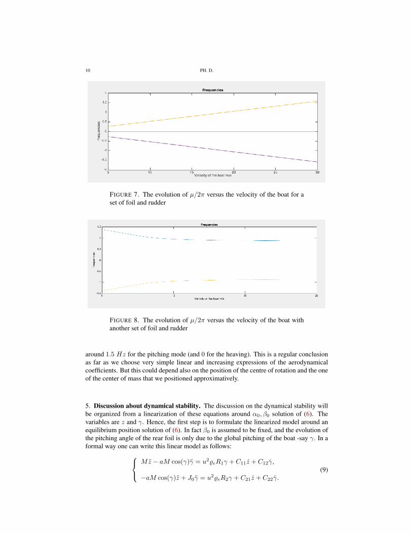
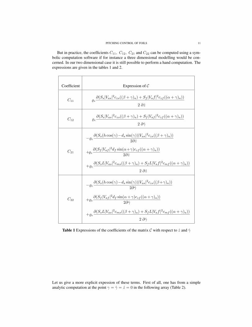
One can observe on figures 7 and 8, that the frequencies are growing with the velocityfor a first set and decreasing for another one. But in both cases the values are similar,

10 PH. D.

FIGURE 7. The evolution of µ/2π versus the velocity of the boat for aset of foil and rudder

FIGURE 8. The evolution of µ/2π versus the velocity of the boat withanother set of foil and rudder

around 1.5 Hz for the pitching mode (and 0 for the heaving). This is a regular conclusionas far as we choose very simple linear and increasing expressions of the aerodynamicalcoefficients. But this could depend also on the position of the centre of rotation and the oneof the center of mass that we positioned approximatively.

5. Discussion about dynamical stability. The discussion on the dynamical stability willbe organized from a linearization of these equations around α0, β0 solution of (6). Thevariables are z and γ. Hence, the first step is to formulate the linearized model around anequilibrium position solution of (6). In fact β0 is assumed to be fixed, and the evolution ofthe pitching angle of the rear foil is only due to the global pitching of the boat -say γ. In aformal way one can write this linear model as follows: Mz − aM cos(γ)γ = u2%eR1γ + C11z + C12γ,

−aM cos(γ)z + J0γ = u2%eR2γ + C21z + C22γ.(9)


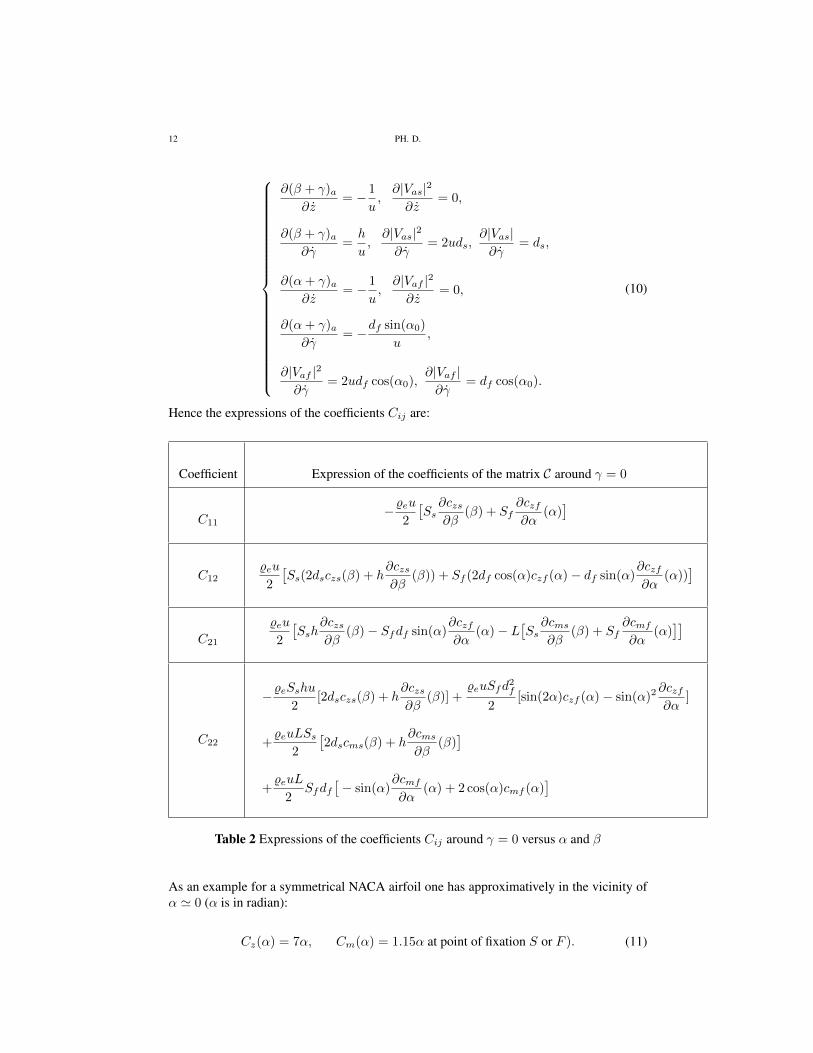
But in practice, the coefficients C11, C12, C21 and C22 can be computed using a sym-bolic computation software if for instance a three dimensional modelling would be con-cerned. In our two dimensional case it is still possible to perform a hand computation. Theexpressions are given in the tables 1 and 2.

Coefficient Expression of C 2

1

C11 %e∂(Ss|Vas|2czs((β + γ)a) + Sf |Vaf |2czf ((α+ γ)a))

2

12 ∂z

C12 %e∂(Ss|Vas|2czs((β + γ)a) + Sf |Vaf |2czf ((α+ γ)a))

2

12 ∂γ

C21

−%e∂(Ss(h cos(γ)−ds sin(γ))|Vas|2czs((β + γ)a))

2∂z

+%e∂(Sf |Vaf |2df sin(α+γ)czf ((α+ γ)a))

2∂z

+%e∂(SsL|Vas|2cms((β + γ)a) + SfL|Vaf |2cmf ((α+ γ)a))

2

12 ∂z

C22

−%e∂(Ss(h cos(γ)−ds sin(γ))|Vas|2czs((β+γ)a))

2∂γ

+%e∂(Sf |Vaf |2df sin(α+ γ)czf ((α+ γ)a))

2∂γ

+%e∂(SsL|Vas|2cms((β + γ)a) + SfL|Vaf |2cmf ((α+ γ)a))

2

12 ∂γ

Table 1 Expressions of the coefficients of the matrix C with respect to z and γ

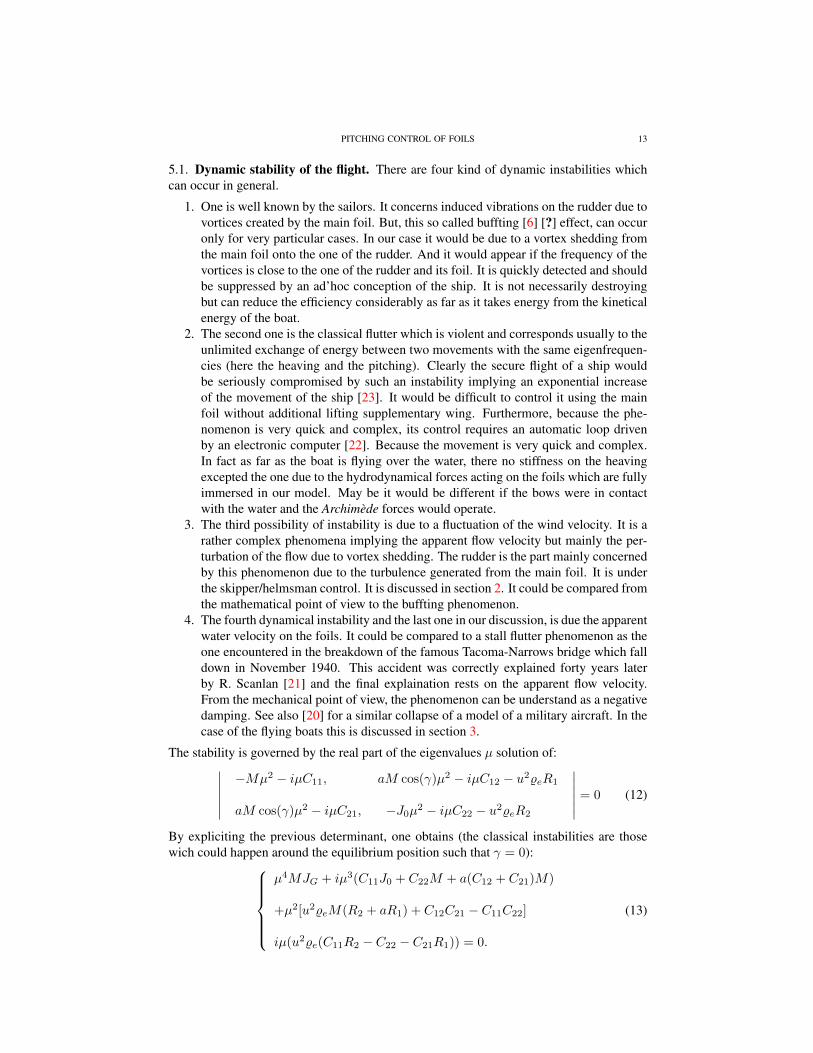
Let us give a more explicit expession of these terms. First of all, one has from a simpleanalytic computation at the point γ = γ = z = 0 in the following array (Table 2).

12 PH. D.

∂(β + γ)a∂z

= − 1

u,∂|Vas|2

∂z= 0,

∂(β + γ)a∂γ

=h

u,∂|Vas|2

∂γ= 2uds,

∂|Vas|∂γ

= ds,

∂(α+ γ)a∂z

= − 1

u,∂|Vaf |2

∂z= 0,

∂(α+ γ)a∂γ

= −df sin(α0)

u,

∂|Vaf |2

∂γ= 2udf cos(α0),

∂|Vaf |∂γ

= df cos(α0).

(10)

Hence the expressions of the coefficients Cij are:

Coefficient Expression of the coefficients of the matrix C around γ = 02

1

C11−%eu

2

[Ss∂czs∂β

(β) + Sf∂czf∂α

(α)]

C12%eu

2

[Ss(2dsczs(β) + h

∂czs∂β

(β)) + Sf (2df cos(α)czf (α)− df sin(α)∂czf∂α

(α))]

C21

%eu

2

[Ssh

∂czs∂β

(β)− Sfdf sin(α)∂czf∂α

(α)− L[Ss∂cms∂β

(β) + Sf∂cmf∂α

(α)]]

C22

−%eSshu2

[2dsczs(β) + h∂czs∂β

(β)] +%euSfd

2f

2[sin(2α)czf (α)− sin(α)2

∂czf∂α

]

+%euLSs

2

[2dscms(β) + h

∂cms∂β

(β)]

+%euL

2Sfdf

[− sin(α)

∂cmf∂α

(α) + 2 cos(α)cmf (α)]

Table 2 Expressions of the coefficients Cij around γ = 0 versus α and β

As an example for a symmetrical NACA airfoil one has approximatively in the vicinity ofα ' 0 (α is in radian):

Cz(α) = 7α, Cm(α) = 1.15α at point of fixation S or F ). (11)


5.1. Dynamic stability of the flight. There are four kind of dynamic instabilities whichcan occur in general.

1. One is well known by the sailors. It concerns induced vibrations on the rudder due tovortices created by the main foil. But, this so called buffting [6] [?] effect, can occuronly for very particular cases. In our case it would be due to a vortex shedding fromthe main foil onto the one of the rudder. And it would appear if the frequency of thevortices is close to the one of the rudder and its foil. It is quickly detected and shouldbe suppressed by an ad’hoc conception of the ship. It is not necessarily destroyingbut can reduce the efficiency considerably as far as it takes energy from the kineticalenergy of the boat.

2. The second one is the classical flutter which is violent and corresponds usually to theunlimited exchange of energy between two movements with the same eigenfrequen-cies (here the heaving and the pitching). Clearly the secure flight of a ship wouldbe seriously compromised by such an instability implying an exponential increaseof the movement of the ship [23]. It would be difficult to control it using the mainfoil without additional lifting supplementary wing. Furthermore, because the phe-nomenon is very quick and complex, its control requires an automatic loop drivenby an electronic computer [22]. Because the movement is very quick and complex.In fact as far as the boat is flying over the water, there no stiffness on the heavingexcepted the one due to the hydrodynamical forces acting on the foils which are fullyimmersed in our model. May be it would be different if the bows were in contactwith the water and the Archimède forces would operate.

3. The third possibility of instability is due to a fluctuation of the wind velocity. It is arather complex phenomena implying the apparent flow velocity but mainly the per-turbation of the flow due to vortex shedding. The rudder is the part mainly concernedby this phenomenon due to the turbulence generated from the main foil. It is underthe skipper/helmsman control. It is discussed in section 2. It could be compared fromthe mathematical point of view to the buffting phenomenon.

4. The fourth dynamical instability and the last one in our discussion, is due the apparentwater velocity on the foils. It could be compared to a stall flutter phenomenon as theone encountered in the breakdown of the famous Tacoma-Narrows bridge which falldown in November 1940. This accident was correctly explained forty years laterby R. Scanlan [21] and the final explaination rests on the apparent flow velocity.From the mechanical point of view, the phenomenon can be understand as a negativedamping. See also [20] for a similar collapse of a model of a military aircraft. In thecase of the flying boats this is discussed in section 3.

The stability is governed by the real part of the eigenvalues µ solution of:∣∣∣∣∣∣−Mµ2 − iµC11, aM cos(γ)µ2 − iµC12 − u2%eR1

aM cos(γ)µ2 − iµC21, −J0µ2 − iµC22 − u2%eR2

∣∣∣∣∣∣ = 0 (12)

By expliciting the previous determinant, one obtains (the classical instabilities are thosewich could happen around the equilibrium position such that γ = 0):

µ4MJG + iµ3(C11J0 + C22M + a(C12 + C21)M)

+µ2[u2%eM(R2 + aR1) + C12C21 − C11C22]

iµ(u2%e(C11R2 − C22 − C21R1)) = 0.

(13)

14 PH. D.

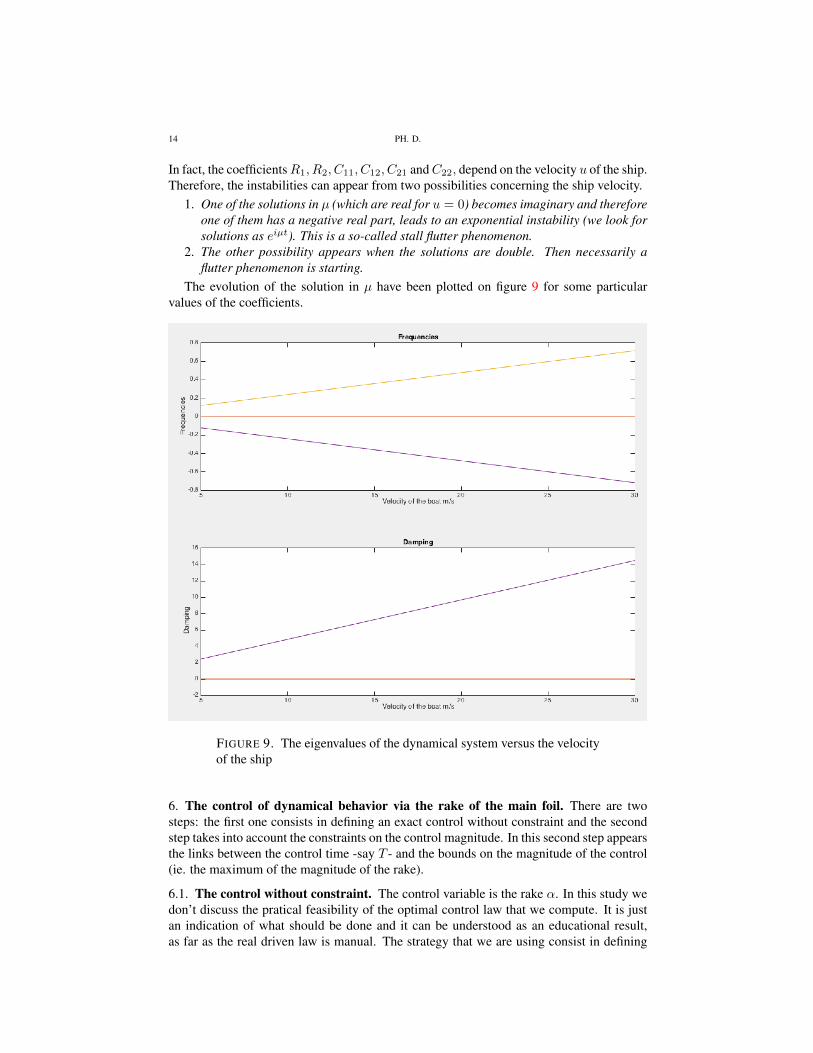
In fact, the coefficientsR1, R2, C11, C12, C21 andC22, depend on the velocity u of the ship.Therefore, the instabilities can appear from two possibilities concerning the ship velocity.

1. One of the solutions in µ (which are real for u = 0) becomes imaginary and thereforeone of them has a negative real part, leads to an exponential instability (we look forsolutions as eiµt). This is a so-called stall flutter phenomenon.

2. The other possibility appears when the solutions are double. Then necessarily aflutter phenomenon is starting.

The evolution of the solution in µ have been plotted on figure 9 for some particularvalues of the coefficients.

FIGURE 9. The eigenvalues of the dynamical system versus the velocityof the ship

6. The control of dynamical behavior via the rake of the main foil. There are twosteps: the first one consists in defining an exact control without constraint and the secondstep takes into account the constraints on the control magnitude. In this second step appearsthe links between the control time -say T - and the bounds on the magnitude of the control(ie. the maximum of the magnitude of the rake).

6.1. The control without constraint. The control variable is the rake α. In this study wedon’t discuss the pratical feasibility of the optimal control law that we compute. It is justan indication of what should be done and it can be understood as an educational result,as far as the real driven law is manual. The strategy that we are using consist in defining


a control criterion and to minimize it with respect to the control variable. This controlcriterion is a norm of the gap between the observed state variables at a time T (pitchingand heaving) and the desired values of these functions. Furthermore we make use of alinearized approximation of the state equation.

Therefore the control problem consists in defining a criterion depending on the statevariables (ie. z and γ) but also on the control δ = α − α0 and to minimize it with respectto δ. Let us first define a delay -say T - corresponding to the reaction time required in thecontrol process. Our goal is to define a control law such that at time T the ship is back tothe equilibrium

z(T ) = z0, z(T ) = γ(T ) = γ(T ) = 0.

Let us set:

M =

M, −aM

−aM, J0

, C =

C11, C12

C21, C22

, X =

z

γ

,

K =

0, −u2%eR1

0, −u2%eR2

, B =

%eu2G1

%eu2G2

, E =

E1 = %euH1

E2 = %euH2

,

where we have introduced the notations:

G1 =Sf

2

∂czf∂γ

(α0),

G2 =Sf2

[L∂cmf∂γ

(α0) + df sin(α0)∂czf∂γ

(α0) + df cos(α0)czf (α0)],

H1 =Sf2

[2df cos(α0)czf (α0)− df sin(α0)

∂czf∂γ

(α0)],

H2 =Sfdf

2

[df (sin(2α0)czf (α0)− sin(α0)2

∂czf∂γ

(α0)

+L(− sin(α0)∂cmf

∂γ (α0) + 2 cos(α0)cmf (α0))].

(14)

This criterion for the control problem, is defined as follows for each value of the positiveparameter ε representing the unitary cost of the control, by (a0, b0, ε are positive numbers):

Jε(δ)=1

2{|z(T )−z0|2+|z(T )|2+|γ(T )|2+|γ(T )|2+ε

∫ T

0

[a0δ2(s)+b0δ

2(s)]ds,

MX − CX +KX = Bδ + E δ, X(0) = X0, X(0) = X1.

(15)

The optimal control is finally defined as the solution of the following problem:

minδ∈H1

0 (]0,T [)Jε(δ). (16)

The first point is to formulate the optimality relation which is obtained in this case bywriting that the derivative of the criterion Jε with respect to δ is zero. This is quite classical

16 PH. D.

to introduce the adjoint state P solution of the following differential system:

MP +tCP +tKP = 0,

MP (T ) =

z(T )

γ(T )

, MP (T ) = −

z(T )− z0

γ(T )

− tCP (T ).(17)

and the optimality relation can be written (see [9],[1]):

∀t ∈]0, T [, tBP − tEP + ε[a0δ − b0δ] = 0,

δ(0) = δ(T ) = 0.(18)

Remark 1. The choice of the space H10 (]0, T [) has been done in order to have a finite

cost for the control δ. The boundary conditions could be different (at t = 0 and t = T ).For instance, with free edge conditions, one would obtain more degrees of freedom forthe control. But the discontinuity at the extremities, is not always a good strategy in thepractical implementation. Nevertheless, this could be useful in particular case where thecontrollability condition is not satisfied. This point is discussed in the following.

2

The solution method can be based on a gradient or more precisely a conjugate gradientmethod using the gradient of Jε which is tBP+εδ. But another much more efficient methodrecently developed, leads to a so-called phase control. Let us explain how to characterizethe corresponding control law.

Let us set a priori: X = X0 + εX1 + . . . ,

P = P 0 + εP 1 + . . . ,

δ = δ0 + εδ1 + . . .

(19)

By introducing a priori these expression into the system (15)-(17)-(18) and bu equattingthe terms of same power in the resulting expressions, one obtains:

• Order 0

MX0 − CX0 +KX0 = Bδ0 + E δ0, X0(0) = X0, X0(0) = X1,

MP 0 +tCP 0 +tKP 0 = 0,

MP 0(T ) = X(T ), MP 0(T ) = −

z0(T )− z0

γ0(T )

− tCP 0(T ),

∀t ∈]0, T [, tBP 0 − tEP 0 = 0,

(20)


• Order 1

MX1 − CX1 +KX1 = Bδ1 + E δ1, X1(0) = 0, X1(0) = 0,

MP 1 +tCP 1 + tKP 1 = 0,

MP 1(T ) = X1(T ), MP 1(T ) = −

z1(T )

γ1(T )

− tCP 1(T ),

[a0δ0 − b0δ0] + tBP 1 − tEP 1 = 0.

(21)

• . . .

Our first point is to prove that with reasonable assumptions, one has P 0 = 0. This is infact an exact controllability result for z0(T ), z0(T ), γ0(T ) and γ0(T ) as it will appear inthe following because it will imply that z0(T ) = z0, z

0(T ) = γ0(T ) = γ0(T ) = 0. Let usnow turn to a controllability result wich is a more adapted version of the general Bellman’sresult [?].

Theorem 6.1. Let us assume that the vectors B, E are linearly independent. Let us intro-duce the dual basis B∗, E∗ defined by ((., .)2 is the scalar product in R2):

(B∗,B)2 = 1, (B∗, E)2 = 0, (E∗, E)2 = 1, (E∗,B)2 = 0.

We set: H =M−1 tC, L =M−1 tK,

Z1 = HB∗, Z2 = HE∗, Z3 = LB∗, Z4 = LE∗.

First of all it is assumed that:

(Z4, E)2 6= 0.

Let ri be the two roots of the following second degree equation:

r2(Z4, E)2 + r[(Z4, E)2(Z1,B)2 − (Z4,B)2(Z1, E)2

]+[(Z4, E)2(Z2,B)2 − (Z4,B)2(Z2, E)2 + (Z4, E)2(Z3,B)2 − (Z4,B)2(Z3, E)2

].

Then, if the roots are such that:

1. If r1 6= r2 (single roots), and if none theses roots is solution of:

i = 1, 2 : r2i[1 + (Z1, E2)

]+ ri

[(Z2, E)2 + (Z3, E)2

]+ (Z4, E)2 = 0.

2. If r1 = r2 (double roots) in addition to the previous condition, r1 should be suchthat:

r21[1 + (Z1, E)2

]− (Z4, E)2 6= 0,

the solution P 0 is zero.As a consequence, from the final conditions satisfied by P 0(T ) and P 0(T ) this implies thatnecessarily one has:

z(T ) = z0, z(T ) = γ(T ) = γ(T ) = 0.

18 PH. D.

ProofThe vector P 0 can be explicited in the dual basis (B∗, E∗) by:

P 0(t) = ξ1(t)B∗ + ξ2(t)E∗.

Therefore:ξ1 + ξ1(Z1,B)2 + ξ2(Z2,B)2 + ξ1(Z3,B)2 + ξ2(Z4,B)2 = 0,

ξ2 + ξ1(Z1, E)2 + ξ2(Z2, E)2 + ξ1(Z3, E)2 + ξ2(Z4, E) = 0,

ξ1 = ξ2.

This implies that:ξ1 + ξ1(Z1,B)2 + ξ1[(Z2,B)2 + (Z3,B)2] + ξ2(Z4,B)2 = 0,

ξ1[1 + (Z1, E)2] + ξ1[(Z2, E)2 + (Z3, E)2] + ξ2(Z4, E) = 0,

ξ1 = ξ2.

Or else:

ξ1(Z4, E)2 + ξ1[(Z4, E)2(Z1,B)2 − (Z4,B)2(Z1, E)2

]+ξ1

[(Z4, E)2((Z2,B)2 + (Z3,B)2)− (Z4,B)2((Z2, E)2 + (Z3, E)2)

]= 0,

ξ1[1 + (Z1, E)2] + ξ1[(Z2, E)2 + (Z3, E)2] + ξ2(Z4, E)2 = 0,

ξ1 = ξ2.

(22)

The solutions of the first above equation are ξ1(t) = Aierit where ri is a root of the

caracteristic equation:

r2(Z4, E)2 + r[(Z4, E)2(Z1,B)2 − (Z4,B)2(Z1, E)2

]+[(Z4, E)2(Z2,B)2 − (Z4,B)2(Z2, E)2 + (Z4, E)2(Z3,B)2 − (Z4,B)2(Z3, E)2

].

Hence, assuming in a first step that the roots are single: ξ2(t) =Airierit + c0 (constant).

Introducing this result into the second equation (22), one obtains for each of the three

sets of solutions: i = 1, 2 : (erit,erit

ri), (0, c0) the necessary relations:

i = 1, 2 : r2i[1 + (Z1, E2)

]+ ri

[(Z2, E)2 + (Z3, E)2

]+ (Z4, E)2 = 0,

and:

(Z4, E)2 = 0.

(23)

Finally, if none of these three relations is satisfied it implies that:

∀t ∈ [0, T ] : ξ1(t) = ξ2(t) = 0 => ∀t ∈ [0, T ] : P 0(t) = 0.


The theorem is proved. Let us discuss now what happens if the rootsof (22) are double:r1 = r2. The solutions of (22) are now:

ξ1(t) = Aer1t, ξ2(t) =A

r1er1t and ξ1(t) = Bter1t, ξ2(t) = B(rt− 1)

ert

r2. (24)

Hence the additional controllability condition is (one is the same as before):

r21[1 + (Z1, E)2

]− (Z4, E)2 6= 0. (25)

2

Remark 2. The controllability condition given in theorem 6.1 can be discussed in partic-ular cases. For instance let us imagine that the damping matrix C is neglected (thereforeE = 0), and we choose b0 = 0 (hence δ ∈ L2(]0, T [). We loose the possibility to prescribethe boundary conditions on δ. Let us introduce a vector E orthogonal to B and such that(E , E)2 = 1. The last relation (20) implies that:

P 0(t) = ξ(t)E .

But the equation satisfied by P 0 leads to:ξ (M−1 tKE ,B)2 = 0,

ξ + ξ (M−1 tKE , E)2 = 0,

and therefore if:

(M−1 tKE ,B)2 6= 0

one can claim that the system can be exactly controlled by a function δ0 that we will definein the following. This condition is simplier than the one with a damping, but it is lessrealistic as far as the velocities are such that the damping is not negligible.

2

Remark 3. If there was no rudder, the matrix K which has only the second row differentfrom zero, is reduced to the vector B. Hence one has tKE∗ = 0. Or else Z4 = 0. One cancheck easily that the controllability requirements are not satisfied in such a case and this isnot surprising.

2

6.2. Characterization of the exact control δ0. In order to define δ0 ∈ H10 (]0, T [) we

make use of the system of order one in ε. We know from this system of relations, that :

a0δ0 − b0δ0 = −tBP 1 + tEP 1, δ0(0) = δ0(T ) = 0,

but P 1 is still unknown and the next step is to compute it.Let us introduce a vector Q depending on the time variable, and such that:

MQ+tCQ+tKQ = 0, Q(0) = δΦ1, Q(0) = Φ2. (26)

20 PH. D.

By multiplying the equation of order zero by Q and by integrating from 0 to T , one obtains(taking into account that X0(T ) = X(T ) = 0):

∫ T

0

(MX0, Q)2 −∫ T

0

(CX0, Q)2 +

∫ T

0

(KX0, Q)2

= −(MX0(0), Q(0))2 + (MX0(0), Q(0))2 + (CX0(0), Q(0))2

=

∫ T

0

[(B, Q)2 − (E , Q)2]δ0.

The control δ0 can be obtained in different ways. One consists in using Fourier series andthis leads to:

δ0(t) =2

T

∑n≥0

An sin(nπt

T),

with:

An =−

∫ T

0

[(B, P 1)2(s)−(E , P 1)2(s)] sin(nπs

T)ds

a0 + b0n2π2

T 2

.

(27)

But δ0 can also be computed from (20) as follows in order to avoid the difficulties connectedwith the Gibbs phenomenon in the Fourier series:

δ0(t) = A0 cosh(rt) +B0 sinh(rt) +

∫ t

0

f(s) sinh(r(t− s))ds,

with:

r =

√a0b0, B0 = −

∫ T

0

f(s) sinh(r(t− s))ds

sinh(rT ), A0 = 0,

f(s) =(B, P 1(s))2 − (E , P 1(s))2

b0r.

(28)

Let us set, choosing for instance, the expression given by the Fourier series:

Φ = (P 1(0), P 1(0)), δΦ = (Q(0), Q(0)),

G1(s) = (B, Q1)2(s)−(E , Q1)2(s), Bn = −∫ T

0

G1(s) sin(nπs

T)ds,

Λ(Φ, δΦ) =2

T

∑n≥0

AnBn,

L(δΦ) = (MX0(0), Q(0))2 − (MX0(0), Q(0))2 − (CX0(0), Q(0))2,

(29)

and the problem to be solved in order to characterize Φ and therefore the exact control δ0;consists in finding the solution of:

Φ ∈ R2 × R2, ∀δΦ ∈ R2 × R2, Λ(Φ, δΦ) = L(δΦ). (30)


Remark 4. The expression of Λ(., .) can also be obtained using the other expression of δ0

given at (28) with more accuracy from the numerical point of view.

Let us now check the solvency of (30). The bilinear form Λ is clearly symmetrical andpositive. The continuity is also straightforward. The same is true for the linear form L.Furthermore if Φ ∈ R4 is such that: Λ(Φ,Φ) = 0 one has (Φ being associated to P 1 in thenext expression):

∀n ∈ N,∫ T

0

[(B, P 1)2(s)−(E , P 1)2(s)] sin(nπs

T)ds = 0,

which implies that the control δ linked to P 1, is solution of the variational model, whichhas a unique solution:

find δ ∈ H10 (]0, T [) such that:∀v ∈ H1

0 (]0, T [),∫ T

0

a0δv + b0δv = −∫ T

0

[(B, P 1)2(s)−(E , P 1)2(s)]v(s)ds.

(31)

Because this solution can be written:

δ =∑n≥0

An sin(nπt

T),

and because An = 0 one can conclude that δ = 0 and finally that the bilinear form ispositively definite. Hence, the system (30) enables to define Φ uniquely. Conversely ifthe control δ0 is defined at (28) where P 1 is solution of (30), the solution X of the initialsystem, satisfies because of (30) (Xd is the vecteur of R2 where only the first componentis different from zero and equal to z0):

(M(X0(T )−Xd), Q(T )) = (MX0(T )− CX0(T ), Q(T )) = 0. (32)

where Q is solution of:∀(Q0, Q1) ∈ R4, Q being solution of

Q(0) = (Q0, Q1), MQ+ tCQ+KQ = 0,(33)

But (Q(T ), Q(T )) can reach any values in R4 as far as one can prescribe any value on theinitial condition for Q. Therefore, this implies that:

z0(T ) = z0, z0(T ) = γ0(T ) = γ0(T ) = 0. (34)

This proves that the control δ0 is exact. Let us summarize the obtained results in thefollowing statement.

Theorem 6.2. Let us assume the hypothesis of theorem 6.1. The bilinear form Λ(., .)defined on R2 × R2 at equation (29) is associated to a symmetrical and positively definitematrix with dimension 4 × 4 -say G. The linear form L is associated to a vector of R4

denoted by L. The following linear equation has a unique solution:

GΦ = L,

and if P 1 is the solution of:

MP 1 + tCP 1 + tKP 1 = 0, (P 1(0), P 1(0)) = Φ.

22 PH. D.

With this set of initial conditions, the function δ0 given (for instance), at (31) is an exactcontrol, depending on the control time T and the initial conditions (X(0), X(0)). Further-more, δ0 is the unique exact control in the space H1

0 (]0, T [) wich minimizes the norm:

v ∈ H10 (]0, T [)→

√a0

∫ T

0

v2 + b0

∫ T

0

v2

.

Proof The only point which remains to be justified, concerns the last point of the state-ment of the theorem. Let us first denote by Uad the convex set (not a vectorial space)defined by: U

ad = {v ∈ H10 (]0, T [), Y (T ) = Y (T ) = 0},

where Y is solution of the second equation (15) with the control v.(35)

Hence δ0 ∈ Uad, one can claim that Uad 6= ∅. Furthermore the mapping:

∀v ∈ Uad → a0

∫ T

0

v2 + b0

∫ T

0

v2,

is strictly convex and therefore there is a unique solution -say δ∗- to the problem:

minv∈Uad

1

2[a0

∫ T

0

v2 + b0

∫ T

0

v2].

It is characterized by (see for instance [5]):

∀v ∈ Uad, a0∫ T

0

δ∗(v − δ∗) + b0

∫ T

0

δ∗(v − δ∗) = 0.

But δ0 which is given by (28), where P 1 is solution of (30), also satisfies (because v andδ0 are both exact control):

∀v ∈ Uad, a0∫ T

0

δ0(v − δ0) + b0

∫ T

0

δ0(v − δ0) = 0.

Hence, by setting v = δ0 in the first relation and v = δ∗ in the second one, and adding thetwo obtained equalities, one gets δ0 = δ∗. 2

6.3. A mathematical result on the convergence. Let us introduce the gap variables by:

X = X −X0, P = P − εP 1, δ = δ − δ0. (36)

From the definition of δ and because δ0 is an exact control law, one obtains:Jε(δ) ≤ Jε(δ0) =

1

2[||X0(T )−Xd||22 + ||X0||22 + ε(a0

∫ T

0

|δ0|2 + b0

∫ T

0

|δ|2)]

=ε

2(a0

∫ T

0

|δ0|2 + b0

∫ T

0

δ2).

And therefore (|| . ||1,2,]0,T [ is the norm used in the space H10 (]0, T [)):

∀ε > 0, ||δ||1,2,]0,T [ ≤ ||δ0||1,2,]0,T [ = constant versus ε.


This enables one to deduce that there is a subsequence (with respect to ε) still denoted byδ such that (using the weak lower semi-continuity for convex functions):

limε→0

δ = δ∗ ∈ H10 (]0, T [)− weak and:

a0||δ∗||20,]0,T [ + b0||δ∗||20,]0,T [ ≤ a0||δ0||20,]0,T [ + b0||δ0||20,]0,T [.

From:

a0||δ − δ∗||20,]0,T [ + b0||δ − δ∗||20,]0,T [ =

a0||δ||20,]0,T [ + b0||δ||20,]0,T [ − 2a0

∫ T

0

δδ∗ − 2b0

∫ T

0

δδ∗ + a0||δ∗||2 + b0||δ∗||20,]0,T [

≤ 2a0

∫ T

0

δ∗(δ∗ − δ) + 2b0

∫ T

0

δ∗(δ∗ − δ)→ε→0 0,

we deduce the strong convergence of δ to δ∗ when ε → 0 and therefore the one of thecorresponding subsequence (X(T )−Xd, X(T )) to (0, 0), because of the continuity of thestate variable with respect to the control law.In addition one has (lower semi-continuity of continuous convex functions):

∀v ∈ H10 (]0, T [), a0||δ∗||20,]0,T [ + b0||δ∗||20,]0,T [ = lim

ε→0Jε(δ) ≤ Jε(v),

and in particular if v ∈ Uad, one gets:

a0||δ∗||20,]0,T [ + b0||δ∗||20,]0,T [ ≤ a0||v||20,]0,T [ + b0||v||20,]0,T [,

which proves (Tychonov’s result [19]) that the control δ∗ minimizes the norm:

v → a0||v||20,]0,T [ + b0||v||20,]0,T [,

and therefore it is precisely the control δ0 found by the asymptotic expansion. Hence thereis only one accumulation point to the sequence δ which converges to δ0 when ε → 0. Letus summarize the obtained result in the next statement.

Theorem 6.3. Let us assume the hypothesis of theorem 6.1. Then there exists a uniqueexact control for a given time control T and for any initial conditions which realizes theminimum of the norm:

v → a0||v||20,]0,T [ + b0||v||20,]0,T [,

in the space H10 (]0, T [) among the exact control. This control -say δ0- is the one given in

theorem 6.2.

Remark 5. The exact control depends on the data ad on the time delay T . But the smallestis T the larger will be the magnitude of the control. And because there is a limitation onthe amplitude of the rake (which is the control), it is necessary to discuss the effect of aconstraint on the control. This is the goal of the next section.

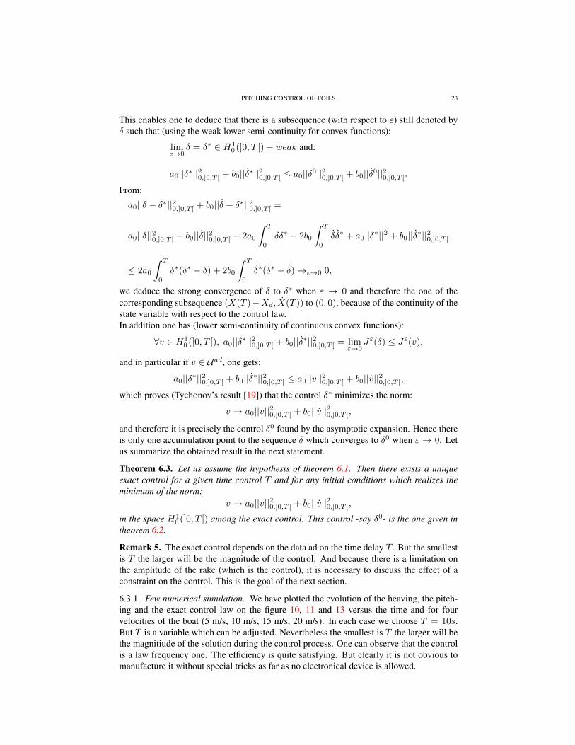
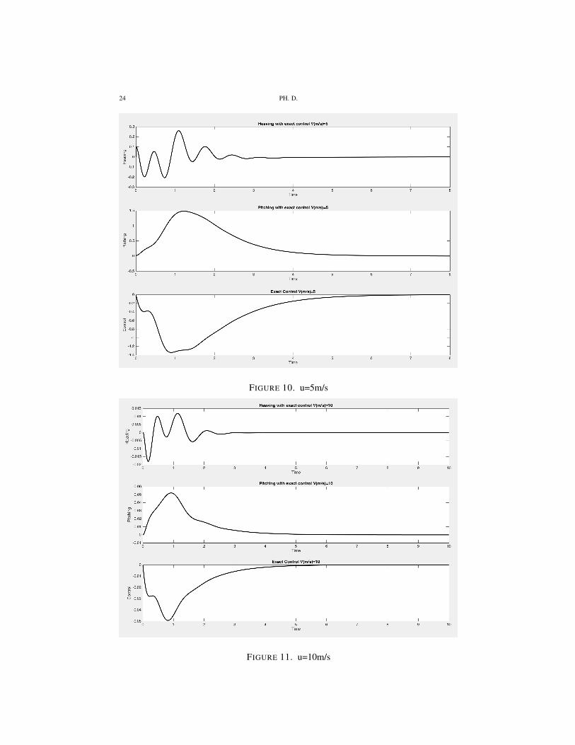
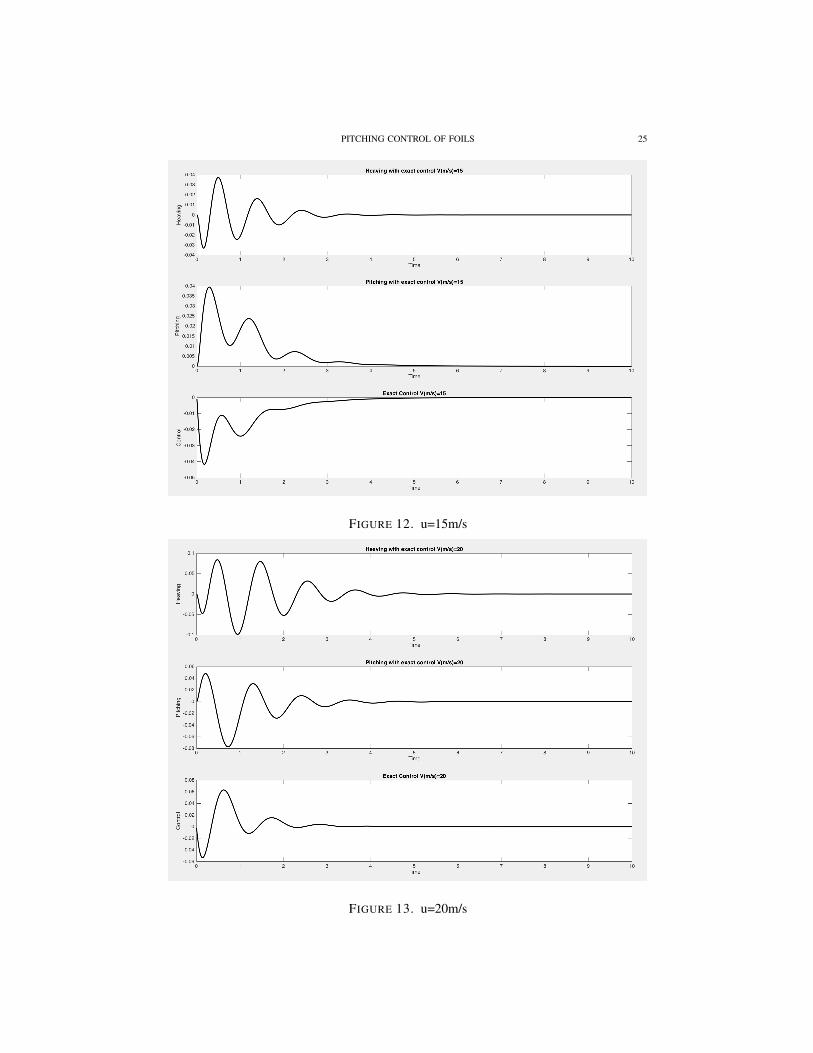
6.3.1. Few numerical simulation. We have plotted the evolution of the heaving, the pitch-ing and the exact control law on the figure 10, 11 and 13 versus the time and for fourvelocities of the boat (5 m/s, 10 m/s, 15 m/s, 20 m/s). In each case we choose T = 10s.But T is a variable which can be adjusted. Nevertheless the smallest is T the larger will bethe magnitiude of the solution during the control process. One can observe that the controlis a law frequency one. The efficiency is quite satisfying. But clearly it is not obvious tomanufacture it without special tricks as far as no electronical device is allowed.

24 PH. D.

FIGURE 10. u=5m/s

FIGURE 11. u=10m/s


FIGURE 12. u=15m/s

FIGURE 13. u=20m/s

26 PH. D.

6.4. Control with constraints. In practice the magnitude of the control is restricted. There-fore the minimisation of the criterion Jε should be performed over the bounded set:

K = {q ∈ H10 (]0, T [), such that: |q| ≤ qmax}. (37)

The new control problem is now:minδ∈K

Jε(δ). (38)

From classical results in optimisation, the optimal solution is characterized by: δ ∈ K,

ae t ∈]0, T [, ∀q ∈ K, Gε(δ)(q − δ) ≥ 0,(39)

or else, by expliciting the gradient of Jε: ae t ∈]0, T [, ∀q ∈ K, (ε[a0δ − b0δ] +tBP −tEP )(q − δ) ≥ 0,

∀q ∈ R, |q| ≤ qmax, δ(T )(q − δ(T )) ≥ 0, δ(T )(q − δ(T )) ≤ 0.

(40)

For ε → 0 one can define a limit control problem (see [20]) following the same ideaas in the previous section, but with a different strategy. Let us consider two followingpossibilities.

6.4.1. Assuming that there is an exact control -say δ0 ∈ K for the initial conditions andthe time control T . In this case one has (δ ∈ K is the unique solution of (38) and is suchthat:

δ ∈ K, ∀v ∈ K, Jε(δ) ≤ Jε(v),

and by choosing v = δ0:a0||δ||20,]0,T [ + b0||δ||20,]0,T [ ≤ a0||δ

0||20,]0,T [ + b0||δ0||20,]0,T [

and

||X(T )−Xd||22 + ||X(T )||22 ≤ Cε.

Hence, δ is bounded in the space H1(]0, T [) and one can extract a subsequence (withrespect to ε but we keep the notation ε because there is no ambiguıty) such that:

limε→0

δ = δ∗ in the space H10 (]0, T [)− weak.

Furthermore one can ensure that:

limε→0||X(T )−Xd||22 + ||X(T )||22 = 0.

But X as function of the space [C2([0, T ])]2 depends continuously of δ as a function ofH1(]0, T [). HenceX tends toX∗ solution obtained with the control δ∗ and therefore satis-fies: X∗(T ) = 0, X∗(T ) = 0. Hence δ∗ is an exact control with the minimum norm usedon H1(]0, T [). Because it is unique (the norm is strictly convex) all the sequence δ con-verges weakly in H1(]0, T [) to δ∗. The adjoint state P tends also in the space [C1([0, T ])]2

to zero because it depends continuously on the final condition. And therefore limε→0

P = 0

in C1([0, T ])-strongly (and even more). One can also prove easily (as previously) that theconvergence of the control δ to δ0 is strong in the space H1

0 (]0, T [).


6.4.2. Assuming that there is no exact control in K for the initial conditions and the timecontrol T . The control δ ∈ K is still bounded in L2(]0, T [) and there is a subsequencestill denoted by δ such that lim

ε→0δ = δ∗ in L2(]0, T [) − weak. Following the justification

given above, one can also claim that the corresponding subsequence of P tends to P ∗ in[C1([0, T ])]2. And P ∗ 6= 0 or else one would have X∗(T ) −Xd = X∗(T ) = 0, which isexcluded by hypothesis or else one would have δ∗ ∈ K and it would be an exact control.From (40) one can state that:

∀q ∈ K,∫ T

0

tBP ∗(q − δ∗) ≥ 0.

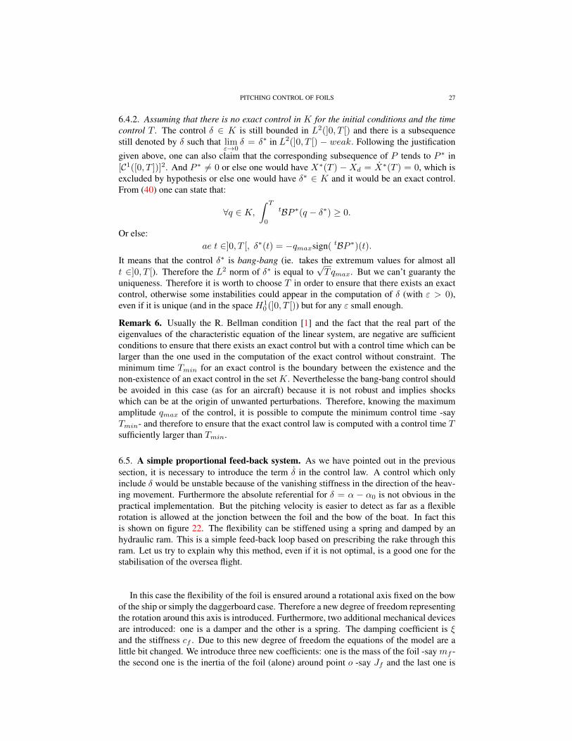
Or else:ae t ∈]0, T [, δ∗(t) = −qmaxsign( tBP ∗)(t).

It means that the control δ∗ is bang-bang (ie. takes the extremum values for almost allt ∈]0, T [). Therefore the L2 norm of δ∗ is equal to

√Tqmax. But we can’t guaranty the

uniqueness. Therefore it is worth to choose T in order to ensure that there exists an exactcontrol, otherwise some instabilities could appear in the computation of δ (with ε > 0),even if it is unique (and in the space H1

0 (]0, T [)) but for any ε small enough.

Remark 6. Usually the R. Bellman condition [1] and the fact that the real part of theeigenvalues of the characteristic equation of the linear system, are negative are sufficientconditions to ensure that there exists an exact control but with a control time which can belarger than the one used in the computation of the exact control without constraint. Theminimum time Tmin for an exact control is the boundary between the existence and thenon-existence of an exact control in the set K. Neverthelesse the bang-bang control shouldbe avoided in this case (as for an aircraft) because it is not robust and implies shockswhich can be at the origin of unwanted perturbations. Therefore, knowing the maximumamplitude qmax of the control, it is possible to compute the minimum control time -sayTmin- and therefore to ensure that the exact control law is computed with a control time Tsufficiently larger than Tmin.

6.5. A simple proportional feed-back system. As we have pointed out in the previoussection, it is necessary to introduce the term δ in the control law. A control which onlyinclude δ would be unstable because of the vanishing stiffness in the direction of the heav-ing movement. Furthermore the absolute referential for δ = α − α0 is not obvious in thepractical implementation. But the pitching velocity is easier to detect as far as a flexiblerotation is allowed at the jonction between the foil and the bow of the boat. In fact thisis shown on figure 22. The flexibility can be stiffened using a spring and damped by anhydraulic ram. This is a simple feed-back loop based on prescribing the rake through thisram. Let us try to explain why this method, even if it is not optimal, is a good one for thestabilisation of the oversea flight.

In this case the flexibility of the foil is ensured around a rotational axis fixed on the bowof the ship or simply the daggerboard case. Therefore a new degree of freedom representingthe rotation around this axis is introduced. Furthermore, two additional mechanical devicesare introduced: one is a damper and the other is a spring. The damping coefficient is ξand the stiffness cf . Due to this new degree of freedom the equations of the model are alittle bit changed. We introduce three new coefficients: one is the mass of the foil -say mf -the second one is the inertia of the foil (alone) around point o -say Jf and the last one is

28 PH. D.

FIGURE 14. Exact control with upper bound on the magnitude of thecontrol. The projection on the admissible set for the control is performedusing the cut off method. One has on this figure V=20 m/s and the initialperturbation is large.

the distance between the point o and the center of mass of the foil (alone) -say dog-; theyare represented on figure 16. The equations of the movement are now (we use the samenotations as before excepted that Jo and M are respectively the inertia and the mass of the


FIGURE 15. Exact control with upper bound on the magnitude of thecontrol. There is no oscillation at the end. The maximum magnitude ofthe control can be adjusted but one can also modify the coefficients a0and b0 and also add a transient term in the control criterion. Here onehas V=20 m/s and the initial perturbation is smaller than the one on theprevious figure.

ship around point o without the main foil):

(M +mf )z − aMγ + dog sin(α0)mf α− c11z − c12(γ + α)

+%Su2

2R1(γ + α) = 0,

−aMz + J0γ − c21z − c22(γ + α) +%SLu2

2R2(γ + α) = 0,

dog sin(α0)mf z + Jf α− c21z − c22γ + (ξ − c22)α

+%LSu2

2R2(γ + α) + cfα = 0.

(41)

30 PH. D.

FIGURE 16. The notations used in this section

Let us introduce new notations for the different matrices:

M =

M +mf −aM dog sin(α0)mf

−aM J0 0

dog sin(α0)mf 0 Jf

C=

c11 c12 c12

c21 c22 c22

c21 c22 c22 − ξ

K =

0%Su2

2R1

%Su2

2R1

0%LSu2

2R2

%LSu2

2R2

0%LSu2

2R2

%LSu2

2R2 + cf

X =

z

γ

α

.

(42)

The equation (42) can therefore be written as follows (with initial conditions):

MX − CX +KX = 0.

The strong stability of the system is obtained as far as the imaginary part of the solution tothe following eigenvalue problem are positive:

det| − λ2M− iλC +K| = 0 (43)

In fact the larger is the least imaginary part of the solution to (43), the best is the stabili-sation of the system. The evolution of the imaginary part of these solutions are plotted onfigure ?? with respect to ξ for various values of cf but with C = 0. One can observe thatthe added spring cf is not necessary for obtaining a stabilisation. In the report publishedby the American team for America’s cup, they mention that this spring was not used (seefigure 7).

6.6. The system used by Oracle Team USA. Let us consider the simple equation, justfor explaining the strategy used, but clearly it has to be adjusted at purpose in pratice:

Jf α+ cfα = −αmaxsign(α), α(0) = α0, α(0) = α1. (44)


This is a very classical control strategy which is often used for stabilizing aircraft. It is notan exact control and the result depends on the value of the maximum amplitude αmax. Butthis can be adjusted easily by a computer on an aircraft and in the case of the America’scup boat, it requires a simple education if the helmsman. One can see on figure 18 howworks the so-called input button which drive αmax by step of ±.50 for each press on thecontrol button. The rest is purely automatic and based on simple mechanical devices. Thesign function is detected by the rocker switch (see figure 22).

The solution have been plotted on figure 17 for height values of αmax. One can see thatthis is stabilized system. The time delay required for the stabilisation depends on both theinitial data and the maximum magnitude αmax of the control.

One could imagine that instead of the control −αmaxsign(α) one set −αmaxsign(α).The results are on figure 17 and show that this doesn’t work at all as it is well know in anycourse in control theory.

FIGURE 17. Several trajectories for different values of αmax startingfrom the same initial condition. One can observe that αmax should beadjusted in order to obain the right control. This is why the helmsmanhas a control box which enables him to adjust αmax by steps of ±.50

FIGURE 18. Several trajectories for different values of αmax startingfrom the same initial condition. One can observe that this control isunuseful. This is why the rocker switcher has to detect the sign of thevelocity of the rake and not the one of the angle (the pitching angle).

32 PH. D.

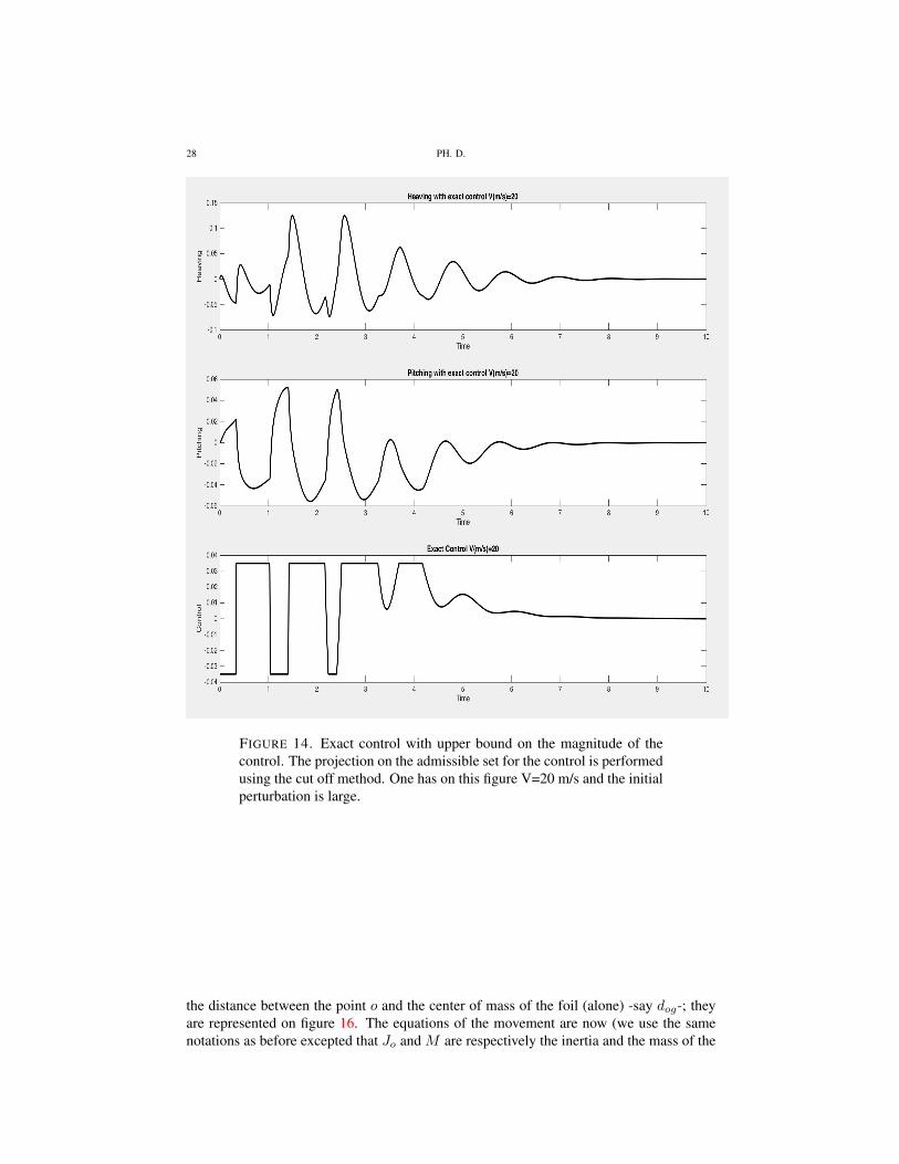
6.7. Comparison between the exact control, OTUSA control and exact control withupper bound. for the same boat and foil-rudder set, we compare the obtained results. Theresults are given on the figures 19, 20 and 21. one can see that the OTUSA system is veryefficient at the beginning but the exact control is more precise for small perturbation. Theideal solution is to couple OTUSA control law at the beginning and the exact control whenthe magnitude of the oscillation are small enough. In this case the mechanical manufactur-ing of the system can be done using a steering box with an additionnal button comparedto the one of OTUSA. But this is another study not included in this analysis. The use of asystem of mass, sring and dashpot can lead to a suitable approximation of the exact feed-back. Because the matrix leading to the exact control with respect to the perturbation isonly dependent on the ship. It is in this study a 4 × 4 symmetrical matrix which thereforedepends on only 10 coefficients. A least square method can be applied in order to give afine approximation of this impedance using a proportional-integral-derivative composed ofseveral mechanical blocks.

FIGURE 19. OTUSA control system. See also figure 17.

7. Conclusion. In this paper, we have suggested a formulation for a simple model in orderto check the controllability of flying boats in a reduced configuration. In fact, only twodegrees of freedom have been considered. The control law is derived from optimal controlfor a vanishing cost parameter (ε→ 0). The controllability is assumed using the theory ofR. Bellman [1]. But a careful study has been necessary because the control system is a partof the stiffness and of the damping matrices. It has been explained and justified that boththe rake angle and its time derivative are involved in the control process.The optimal control laws found in subsections 6.1 and 6.4 are theoretical and can onlybe exactly applied as far as an electronic device coupled with a mechanical actuator, is


FIGURE 20. OTUSA’s system. The magnitude of the control is reducedduring the control process.

used. The comparaison with the control system used by OTUSA shows the theoreticaladvantages of this exact control. But from a practical point of view, it is not obviousthat these advantages would be significant. Because of the regulations in the America’scup, only mechanical devices can be used and the manufacturing of a mechanical systemreproducing the exact control law is not discussed in this paper.Therefore the strategy used by the American Team which is fully compatible with the rules,even if it is not optimal, is an interesting alternative. Nevertheless, much better resultswould be obtained by using slightly different manufacturing of the foil and the rudder. Wedo not explicit these improvements in this paper which are still to be discussed and checked.May be they will be discussed in a futur work.

34 PH. D.

FIGURE 21. Exact control system with bounds on the control magni-tude with the same perturbation as in the the two previous figures withOTUSA control system.

Annex: the mechanical device used by OTUSA

References

[1] R. Bellman [1957], Dynamic programming, Dover edition.[2] J.L. Lions, [1988] Contrôlabilité exacte, perturbations et stabilisation de systèmes distribués, Masson, Paris.[3] Y.C. Fung, [1969], An introduction to the theory of aeroelasticity, Dover publication.[4] E.H. Dowell, H.C. Curtiss Jr., R.H. Scanlan, F. Sisto [1978], A Modern Course in Aeroelasticity. Monographs

and textbooks of solids and fluids. Alphen aan den Rijn, Sijthoff and Noordhoff International Publishers.[5] Jean Cea [1968], Optimisation, Théorie et Algorithmes, Dunod, Paris.[6] Ph. Destuynder [2007], Introduction à l’aéroélasticité et à l’aéroacoustique. Hermès-Lavoisier, Paris-

Londres.[7] Ph. Destuynder [2010], Analyse et contrôle des équations différentielles, Hermès-Lavoisier, Paris-Londres.[8] Ph. Destuynder and M. T. Ribereau [1996], Non linear dynamics of test models in wind tunnels, in Eur. J.

Mech. A/Solids,15,n◦1, p. 91-136.[9] http : //www.naiad.com/ProductF lyerT − Foil.pdf

[10] http : //www.marin.nl/web/Research − Topics/Motions/Ride− control − Foil − assist −craft.htm

[11] http : //www.cupexperience.com/blog/2013/11/ac72− foil − control− system− 2/[12] http : //www.boardrepair.co.uk/downloads/ConSysMoth.pdf

[13] http : //www.gc32racing.com/foils/

[14] http : //www.tandfonline.com/doi/abs/10.1080/14484846.2006.11464502[15] http : //dspace.mit.edu/handle/1721.1/42917

[16] http : //dspace.mit.edu/bitstream/handle/1721.1/42917/245535660−MIT.pdf?sequence =

2[17] http : //www.yachtingworld.com/blogs/matthew−sheahan/americas−cup−what−was−

changed− on− oracle− 555


FIGURE 22. The Oracle USA-Team used this mechanical control to winthe last eight races in a row. In particular, but not only, it enables them tonavigate in the wake of the challenger mainly at the tacking [24].

36 PH. D.

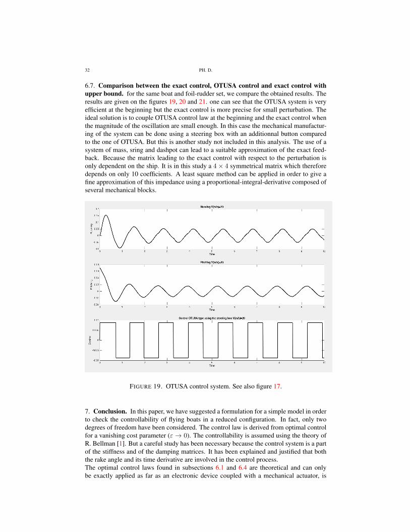
FIGURE 23. Principle of the device used published in [24]

[18] http : //news.mit.edu/2013/qaa− engineering − professors− on− americas− cup

[19] Melina Freitag [20111], http://people.bath.ac.uk/mamamf/talks/ilas.pdf[20] http://aerostudents.com/files/automaticFlightControl/stabilityAugmentationSystems.pdf[21] http://contrails.iit.edu/DigitalCollection/1972/AFFDLTR72-063.pdf[22] http://www.telegraph.co.uk/cars/columnists/andrew-english/sailing-the-ben-ainslie-americas-cup-yacht/[23] https://www.quora.com/[24] http://www.cupexperience.com/blog/2013/11/ac72-foil-control-system-2/

FEW THEORETICAL REMARKS ON THE DYNAMICAL CONTROL …

Documents