INSTITUTE OF PHYSICS PUBLISHING REPORTS ON PROGRESS IN PHYSICS Rep. Prog. Phys. 64 (2001) 701–736 www.iop.org/Journals/rp PII: S0034-4885(01)60525-6 Few-electron quantum dots L P Kouwenhoven 1 , D G Austing 2 and S Tarucha 2,3 1 Department of Applied Physics, DIMES and ERATO Mesoscopic Correlation Project, Delft University of Technology, PO Box 5046, 2600 GA Delft, The Netherlands 2 NTT Basic Research Laboratories, Atsugi-shi, Kanagawa 243-0129, Japan 3 ERATO Mesoscopic Correlation Project, University of Tokyo, Bunkyo-ku, Tokyo 113-0033, Japan Received 3 January 2001, in final form 3 April 2001 Abstract We review some electron transport experiments on few-electron, vertical quantum dot devices. The measurement of current versus source–drain voltage and gate voltage is used as a spectroscopic tool to investigate the energy characteristics of interacting electrons confined to a small region in a semiconducting material. Three energy scales are distinguished: the single-particle states, which are discrete due to the confinement involved; the direct Coulomb interaction between electron charges on the dot; and the exchange interaction between electrons with parallel spins. To disentangle these energies, a magnetic field is used to reorganize the occupation of electrons over the single-particle states and to induce changes in the spin states. We discuss the interactions between small numbers of electrons (between 1 and 20) using the simplest possible models. Nevertheless, these models consistently describe a large set of experiments. Some of the observations resemble similar phenomena in atomic physics, such as shell structure and periodic table characteristics, Hund’s rule, and spin singlet and triplet states. The experimental control, however, is much larger than for atoms: with one device all the artificial elements can be studied by adding electrons to the quantum dot when changing the gate voltage. (Some figures in this article are in colour only in the electronic version; see www.iop.org) 0034-4885/01/060701+36$90.00 © 2001 IOP Publishing Ltd Printed in the UK 701

Welcome message from author
This document is posted to help you gain knowledge. Please leave a comment to let me know what you think about it! Share it to your friends and learn new things together.
Transcript
INSTITUTE OF PHYSICS PUBLISHING REPORTS ON PROGRESS IN PHYSICS
Rep. Prog. Phys. 64 (2001) 701–736 www.iop.org/Journals/rp PII: S0034-4885(01)60525-6
Few-electron quantum dots
L P Kouwenhoven1, D G Austing2 and S Tarucha2,3
1 Department of Applied Physics, DIMES and ERATO Mesoscopic Correlation Project,Delft University of Technology, PO Box 5046, 2600 GA Delft, The Netherlands2 NTT Basic Research Laboratories, Atsugi-shi, Kanagawa 243-0129, Japan3 ERATO Mesoscopic Correlation Project, University of Tokyo, Bunkyo-ku, Tokyo113-0033, Japan
Received 3 January 2001, in final form 3 April 2001
Abstract
We review some electron transport experiments on few-electron, vertical quantum dot devices.The measurement of current versus source–drain voltage and gate voltage is used as aspectroscopic tool to investigate the energy characteristics of interacting electrons confinedto a small region in a semiconducting material. Three energy scales are distinguished: thesingle-particle states, which are discrete due to the confinement involved; the direct Coulombinteraction between electron charges on the dot; and the exchange interaction between electronswith parallel spins. To disentangle these energies, a magnetic field is used to reorganize theoccupation of electrons over the single-particle states and to induce changes in the spin states.We discuss the interactions between small numbers of electrons (between 1 and 20) usingthe simplest possible models. Nevertheless, these models consistently describe a large set ofexperiments. Some of the observations resemble similar phenomena in atomic physics, suchas shell structure and periodic table characteristics, Hund’s rule, and spin singlet and tripletstates. The experimental control, however, is much larger than for atoms: with one device allthe artificial elements can be studied by adding electrons to the quantum dot when changingthe gate voltage.
(Some figures in this article are in colour only in the electronic version; see www.iop.org)
0034-4885/01/060701+36$90.00 © 2001 IOP Publishing Ltd Printed in the UK 701

702 L P Kouwenhoven et al
Contents
Page1. Introduction 7032. Device parameters and experimental setup 7073. Theory 709
3.1. Constant-interaction model 7093.2. Single-particle states in a two-dimensional harmonic oscillator 711
4. Magnetic-field dependence of the ground states 7134.1. Shell filling and Fock–Darwin states 7134.2. Hund’s rule and exchange energy 717
5. Excitation spectrum 7195.1. Coulomb diamonds 7195.2. Excitation stripes 722
6. Limitations of the constant-interaction model 7247. Singlet–triplet transition for N = 2 7268. Experimental determination of direct Coulomb and exchange interactions 7289. Conclusions 734
Acknowledgments 735References 735

Few-electron quantum dots 703
1. Introduction
Quantum dots are small man-made structures in a solid, typically with sizes ranging fromnanometres to a few microns. They consist of 103–109 atoms with an equivalent numberof electrons. In semiconductors all electrons are tightly bound to the nuclei except for asmall fraction of free electrons. This small number can be anything from a single, freeelectron to a puddle of several thousands in quantum dots defined in a semiconductor. Currentnanofabrication technology allows us to precisely control the size and shape of these dots.The electronic properties of dots show many parallels with those of atoms. Most notably,the confinement of the electrons in all three spatial directions results in a quantized energyspectrum. Quantum dots are therefore regarded as artificial atoms [1]. Since we are interestedin electronic transport, we limit this review to quantum dots that are fabricated between thesource and drain electrical contacts. In such a setup, current–voltage measurements are used toobserve the atom-like properties of the quantum dot. In addition, it is possible to vary the exactnumber of electrons on the dot by changing the voltage applied to a nearby gate electrode. Thiscontrol allows one to scan through the entire periodic table of artificial elements by simplychanging the voltage.
The symmetry of a quantum system is responsible for degeneracies in the energy spectrum.The three-dimensional spherically symmetric potential around atoms yields degeneraciesknown as the shells, 1s, 2s, 2p, 3s, 3p, . . . . The electronic configuration is particularly stablewhen these shells are completely filled with electrons, occurring at the atomic numbers of2, 10, 18, 36, . . . . These are the magic numbers of a three-dimensional spherically symmetricpotential. Up to atomic number 23 the atomic shells are filled sequentially by electrons in asimple manner (i.e. mixing between levels originating from different shells starts at atomicnumber 24). Within a shell, Hund’s rule determines whether a spin-down or a spin-up electronis added [2].
The confinement potential of dots can, to some extend, be chosen at will. Figure 1(c) showsexamples of different shapes that can be fabricated. Here, we will mainly consider the circularpillar, which has the highest degree of symmetry. The quantum dot is inside the pillar and hasthe shape of a two-dimensional disc [3, 4]. The repulsive, confinement potential is rather softand can be approximated by a harmonic potential. (This r2-dependence, instead of the 1/rattractive potential in atoms, has several consequences for the energy spectrum and relaxationtimes [5].) The symmetry of such a two-dimensional cylindrically symmetric, harmonicpotential leads to a two-dimensional shell structure with the magic numbers 2, 6, 12, 20, . . . .Note that the lower degree of symmetry in two-dimensional structures leads to a lower magicnumber sequence.
In this review we concentrate on the electronic transport properties of few-electronquantum dot devices which contain circular symmetry. In particular, we discuss a coherentset of experiments performed at NTT and Delft University. Many other electron transportexperiments have been performed on planar or lateral devices defined in two-dimensionalelectron gases of semiconductor heterostructures [1, 6]. ([6] also reviews the history of theearly developments in this field, something that we omit here.) In those devices the electronnumber is usually unknown and symmetry is absent. On the other hand, those devices are moreflexible for integration in small quantum circuits and for addressing them by radio-frequencyand microwave signals. The absence of symmetry has also been turned into an advantage byusing them for extensive studies on chaos in quantum systems [7]. Besides semiconductordevices, metallic grains [8] and molecular devices [9] have also exhibited a discrete energyspectrum in electron transport. For all these experiments we refer to the existing reviews [1,6,9]and their references.

704 L P Kouwenhoven et al
Drain
n-GaAs
n-GaAs
AlGaAs
AlGaAsInGaAs
V
Side gate
Dot
I
Source
Drain
~0.5 mµ
eVsdSource
Drain
Source
Drain
Dot
(a) (b)
(c)
sd
Figure 1. (a) Schematic diagram of a semiconductor heterostructure. The dot is located betweenthe two AlGaAs tunnel barriers. A negative voltage applied to the side gate squeezes the dot thusreducing the effective diameter of the dot (dashed curves). (b) Corresponding energy diagram. Inthis case electrons can tunnel from occupied states in the drain via the dot to an empty state in thesource. The source–drain voltage, Vsd, determines the difference in the Fermi energies betweenthe two electrodes. The current is blocked when this energy window lies in-between two states inthe dot. (c) Scanning electron micrographs of quantum dot pillars with various shapes. The pillarshave widths of about 0.5 µm.
Before describing specific experiments, we first introduce the central ideas related toatomic-like properties and explain how these are observed in single-electron transport.Electron tunnelling from the source to dot and from dot to the drain is dominated by anessentially classical effect that arises from the discrete nature of charge. When relatively high-potential barriers separate the dot from the source and drain contacts, tunnelling to and fromthe dot is weak and the number of electrons on the dot, N , will be a well defined integer.A current flowing via a sequence of tunnelling events of single electrons through the dotrequires this number to fluctuate by one. The Coulomb repulsion between electrons on thedot, however, results in a considerable energy cost for adding an extra electron charge. Extraenergy is therefore needed, and no current will flow until increasing the voltage provides thisenergy. This phenomenon is known as Coulomb blockade [10]. To see how this works inpractice, we consider the schematic pillar structure in figure 1(a). The quantum dot is locatedin the centre of the pillar and can hold up to ∼100 electrons. The diameter of the dot is a fewhundred nanometres and its thickness is about 10 nm. The dot is sandwiched between twonon-conducting barrier layers, which separate it from conducting material above and below,i.e. the source and drain contacts. A negative voltage applied to a metal gate around the pillarsqueezes the diameter of the dot’s lateral potential. This reduces the number of electrons, oneby one, until the dot is completely empty.
Due to the Coulomb blockade, the current can flow only when electrons in the electrodeshave sufficient energy to occupy the lowest possible energy state for N + 1 electrons on thedot (figure 1(b)). By changing the gate voltage, the ladder of the dot states is shifted throughthe Fermi energies of the electrodes. This leads to a series of sharp peaks in the measuredcurrent (figure 2(a)). At any given peak, the number of electrons alternates between N and

Few-electron quantum dots 705
-1.5 -0.80
20
2 126N=0CU
RR
EN
T(p
A)
GATE VOLTAGE (V)
}e /C E2 +∆
1 32 4 5 6 7
}
e /C2
}e /C2
}
e /C2
}
e /C2
}
e /C E2 +∆
0 10
6
1212
62
Add
ition
ener
gy(m
eV)
N
2
6
8
20
9 10 11 12
1918171613
7
43
1
5Oo
Ha
Ja
Ta
Da1514
To Ho
KoEt
Periodic Table of2D Artificial Atoms
CrMiSa
Au
Wi Fr El
4
9 1616
(a)
(b)
(c)
0 20
Figure 2. Current flowing through a two-dimensional circular quantum dot on varying the gatevoltage. (a) The first peak marks the voltage where the first electron enters the dot, and the numberof electrons, N , increases by one at each subsequent peak. The distance between adjacent peakscorresponds to the addition energies (see inset). (b) The addition of electrons to circular orbits isshown schematically. The first shell can hold two electrons whereas the second shell can containup to four electrons. It therefore costs extra energy to add the third and seventh electron. (c) Theelectronic properties following from a two-dimensional shell structure can be summarized in aperiodic table for two-dimensional elements. (The elements are named after team members fromNTT and Delft.)
N + 1. Between the peaks, the Coulomb blockade keeps N fixed and no current can flow.The distance between consecutive peaks is proportional to the so-called addition energy, Eadd,which is the energy difference between the transition points of (N to N+1) and (N + 1 to

706 L P Kouwenhoven et al
N + 2) electrons. Compared to atomic energy, the addition energy for a dot is equal to thedifference between the ionization energy and the electron affinity [11]. The simplest model fordescribing the energetics is the constant-interaction (CI) model [6,10], which crudely assumesthat the Coulomb interaction between the electrons is independent of N . In this model, theaddition energy is given by Eadd = e2/C +�E, where �E is the energy difference betweenconsecutive quantum states. The Coulomb interactions are represented as a charging energy,e2/C, of a single electron charge, e, on a capacitor C.
Despite its simplicity, this model is remarkably successful in providing an elementaryunderstanding. The first peak in figure 2(a) marks the energy at which the first electron entersthe dot, the second records the entry of the second electron and so on. The spacing betweenpeaks, measured in gate voltage, is directly proportional to the addition energy. Note that thespacing is not constant and significantly more energy is needed to add an electron to a dot with2, 6 and 12 electrons (inset figure 2(a)), i.e. the first few magic numbers for a two-dimensionalcircular harmonic potential.
Figure 2(b) shows the two-dimensional orbits allowed in the dot. The orbit with thesmallest radius corresponds to the lowest energy state. This state has zero angular momentumand, as the s-states in atoms, can hold up to two electrons with opposite spin. The addition ofthe second electron thus only costs the charging energy, e2/C. Extra energy,�E, is needed toadd the third electron since this electron must go into the next energy state. Electrons in thisorbit have an angular momentum ±1 and two spin states so that this second shell can containfour electrons. The sixth electron fills up this shell so that extra energy is again needed to addthe seventh electron.
In atomic physics, Hund’s rule states that a shell is first filled with electrons with parallelspins until the shell is half full. After that filling continues with anti-parallel spins. Inthe case of two-dimensional artificial atoms, the second shell is half filled when N = 4.This maximum spin state is reflected by a somewhat enhanced peak spacing, or additionenergy (inset to figure 2(a)). Half filling of the third and forth shells occur for N = 9 and16. These phenomena can be summarized in a periodic table for two-dimensional elements(figure 2(c)). The rows are shorter than those for three-dimensional atoms due to the lowerdegree of symmetry.
Quantum dots have been shown to provide a two-dimensional analogy for real atoms. Dueto their larger dimensions, dots are suitable for experiments that cannot be carried out in atomicphysics. It is especially interesting to observe the effect of a magnetic field,B, on the atom-likeproperties. A magnetic flux-quantum in an atom typically requires a B-field as high as 106 T,whereas for dots this is of order 1 T. (A flux quantum is h/e = BA, where A is the area of thedot.) The scale of a flux-quantum corresponds to a considerable change in the shape of theorbits. The change in orbital energy is roughly heB/m∗, which is as much as 1.76 meV T−1
in GaAs due to the small effective mass m∗ = 0.067me. A magnetic field has, on the otherhand, a negligible effect on the Zeeman spin splitting, gµBB, which is only ∼0.025 meV T−1
in GaAs, since gGaAs = −0.44. A magnetic field therefore is about 70 times more effectivefor changing the orbital energy than for changing the Zeeman spin splitting in GaAs. Wewill thus neglect Zeeman spin splitting throughout this review. However, the spin does playan important role via Hund’s rule. The associated energy is the exchange energy betweenelectrons with parallel spins. In section 4.2, we extend the so-called CI model to includeHund’s rule. This model, which treats the quantum states, the direct Coulomb interaction andthe exchange interaction separately provides a good introduction to the physics of interactingparticles. When we understand the interactions between a small number of electrons we cangradually increase N and see how many-body interactions arise.

Few-electron quantum dots 707
n =0z
n =1z
0
InG
aAs
AlG
aAs
AlG
aAs
GaA
s
GaA
s
n-G
aAs
n-G
aAs
0-40 40growth direction z (nm)
EF
200
pote
ntia
l(m
V)
500-500
drai
n
sour
ce
Figure 3. Self-consistent calculation of the energy diagram of the unpatterned double-barrierheterostructure from which the pillars are fabricated [14]. The electron density in the contactsgradually increases moving away from the tunnel barriers, which can be seen from the increasingdistance between the Fermi energy and the conduction band edge. The structure is designed suchthat the lowest quantum state in the vertical z-direction is partially occupied and the second statealways stays empty.
2. Device parameters and experimental setup
The pillars in figure 1(c) are in fact three-terminal field-effect transistors. The current throughthe transistor can be switched from on to off by changing the gate voltage. In this type oftransistor there is not just one threshold voltage but a quasi-periodic set of voltages where thecurrent switches. Only a small fraction of a single-electron charge is sufficient to drive theswitch. That is why these devices are named single-electron transistors, or SETs. It is as yetunclear whether SETs will have a commercial impact in future electronics [12].
Our quantum dot SET is a miniaturized resonant tunnelling diode [13]. The pillars areetched from a semiconductor double-barrier heterostructure and a metal gate electrode isdeposited around the pillar. The surface potential together with the gate potential confinesthe electrons in the lateral x- and y-directions while the double-barrier structure providesconfinement in the vertical z-direction (figure 1(a)). The dot is formed in the central well thatis made of undoped In0.05Ga0.95As and has a thickness of 12.0 nm. Undoped Al0.22Ga0.78Aslayers form the tunnel barriers. The upper barrier has a thickness of 9.0 and the lower barrieris 7.5 nm thick. The conducting source and drain contacts are made from Si-doped n-GaAs.The concentration of the Si dopants increases away from the two barriers. It is zero up to 3 nmand then increases stepwise from 0.75 × 10¹⁷ to 2.0 × 1018 cm−3 at 400 nm away from thebarriers. This variation in material and doping leads to the conduction band profile shown infigure 3 [14].
A key ingredient of this heterostructure is the inclusion of 5% indium in the well. Thislowers the bottom of the conduction band in the well to 32 meV below the Fermi levelof the contacts. From the confinement potential in the vertical, z-direction it follows thatthe lowest quantum state in the well is 26 meV above the bottom of the conduction band.This state is thus 6 meV below the Fermi level of the contacts. (The well can in goodapproximation be regarded as a two-dimensional system since the second quantum state inthe z-direction is 63 meV above the Fermi level. These states are never occupied in the

708 L P Kouwenhoven et al
present experiments.) To reach equilibrium, the well is filled with electrons until the highestoccupied state in the dot is as close to as possible, but lower than the Fermi levels in thecontacts. The key feature of this vertical quantum dot system is that it contains electronswithout applying voltages. This allows one to study the linear transport regime; i.e. the currentin response to a very small source–drain voltage, Vsd. In contrast, in previously studiedstructures, GaAs without indium was used as the well material [15, 16]. The lowest state inthe well is then above the Fermi level of the contacts. It is then necessary to apply a largeVsd to force electrons into the well and to obtain a current flow. From these materials two-terminal [15] as well as three-terminal devices [16] have been fabricated. Other techniques,where the barriers are doped with Si, have been successful in accumulating electrons in thewell [17, 18]. The nearby presence of charged donors, however, has the disadvantage ofintroducing strong disorder in the dot. By optimizing the doping profile and using capacitancespectroscopy, Ashoori et al [19] succeeded in measuring the linear response of few-electrondots. These measurements have shown several features that are similar to those discussed inthis review.
The fabrication of the gate around the pillar starts with the definition of a metal circlewith diameter D that will later serve as the top contact. This metal circle is also used as amask for dry etching followed by wet etching to a point just below the region of the doublebarriers. Due to this etching combination, the top metal circle is a bit wider than the body ofthe pillar, as can be seen in figure 1(c). The larger top metal circle thus serves as a shadowmask for the evaporation of the metal gate; only the lower part of the pillar and the surroundingetched semiconductor are covered [3]. When the pillar’s diameter D ≈ 0.5 µm, the numberof electrons is about 80 at zero gate voltage. Upon application of a negative gate voltage, Vg,the electron number, N, decreases one-by-one. At a pinch-off voltage around Vg ≈ −1.5 V,N becomes 0. For larger negative voltages (Vg < ∼ − 2 V) a leakage current starts to flowbetween the gate and the source contact, inhibiting proper operation. It is therefore importantto choose the material parameters properly. The pinch-off voltage is directly related to thetwo-dimensional electron density, ne, in the well of the unpatterned material. Shubnikov–deHaas measurements on large area devices give ne = 1.7×10¹⁵ m−2. This is in good agreementwith self-consistent calculations that give ne = 1.67 × 10¹⁵ m−2. From the electron densitymultiplied by the area we estimate that about 10 electrons are in the dot when the effectivediameter deff = 100 nm. At Vg = 0 where N ≈ 80 the effective diameter is ∼300 nm, whichis considerably smaller than the pillar’s diameter.
It is important to realize that the geometry of these vertical dot devices leads to strongscreening of the Coulomb interactions by the free electrons in the source and drain. These areonly ∼10 nm away, which is much less than the dot’s diameter. Rather then an unscreened1/r-Coulomb potential, the Coulomb interaction between two electrons at opposite edges onthe dot is exponentially screened. (Note that screening occurs via positive image charges in thesource generating negative image charges in the drain contacts, and vice versa. This results innearly exponential screening.) This is illustrated when we compare the self-capacitance of afree disc with the parallel plate capacitors between the dot and contacts. The self-capacitanceof a disc with diameter deff = 100 nm is Cself = 4εrεodeff ≈ 50 aF (εr = 12.7 in GaAs),giving a measure for the unscreened interactions by the charging energy, e2/Cself ≈ 4 meV.The capacitance of a vertical dot is more realistically approximated by two parallel capacitorsbetween the dot and the source and drain leads, C = Cs + Cd = εrεoπd
2eff/(2d) ≈ 200 aF.
Here, d = 10 nm is the thickness of the tunnel barriers. The charging energy for screenedinteractions gives e2/C ≈ 1 meV; a value four times smaller than for the unscreened case.Electrons on the dot will thus have a short-range interaction. The strength of this interactionis further weakened by the finite thickness of the disc.

Few-electron quantum dots 709
An important parameter in classifying the importance of electron–electron interactions isthe ratio between the charging energy and the confinement energy. To estimate the confinementenergy we take a harmonic potential with oscillator frequency ωo. We make the estimate forN ∼ 10 electrons corresponding to a partially filled third shell. By equating the energy atthe classical turning point to the energy of the third shell (1/2m∗ω2
od2eff/4 = 3hωo), we obtain
hωo = 3 meV. This implies that the separation of the single-particle states, i.e. the eigenstatesof non-interacting electrons, is of the same order or even larger than the charging energy.This puts vertical dots in a very different regime compared to lateral quantum dots wherethe separation between single-particle states is typically 5–10 times smaller than the chargingenergy [6].
The measurements in this review are performed at a temperature of 100–200 mK. Below500 mK the temperature has little effect. Above that, the Coulomb peaks start to broaden andthe peak heights decrease. The measurement circuit is shown schematically in figure 1(a). Thecurrent, I , flows vertically through the dot in response to a dc voltage, Vsd, applied betweenthe source and drain contacts. To measure the ground state (GS) energies, a sufficiently smallvoltage is applied to give a linear-response regime. A typical value is Vsd = 100 µV. The gatevoltage, Vg, is typically varied between −2.5 and +0.7 V. Beyond these values leakage occursthrough the Schottky barrier between the gate and the source. A magnetic field can be appliedup to 16 T, directed parallel to the current.
One aspect worth noting about the pillar devices is that the measurements generallyreproduce in great detail. In all the more or less 20 devices measured with D between 0.4and 0.54 µm, large addition energies are found for N = 2 and 6. In about 10 of these a largeaddition energy is also observed forN = 12. Hund’s rule states are often observed forN = 4,and 9, and sometimes also for N = 16. Traces like the one shown in figure 2(a) reproducein detail, even after we cycle the device several times to room temperature. (To be precise,the peak spacings and heights reproduce in detail, but not the precise gate voltages where thepeaks occur.) This degree of reproducibility, which is on the level with single-particle states,is unprecedented in solid-state devices.
3. Theory
3.1. Constant-interaction model
In this section we introduce the CI model that provides an approximate description of theelectronic states of quantum dots [6, 10, 20]. The CI model is based on two importantassumptions. First, the Coulomb interactions of an electron on the dot with all other electrons,in and outside the dot, are parametrized by a constant capacitance C. Second, the discrete,single-particle energy spectrum, calculated for non-interacting electrons, is unaffected by theinteractions. The CI model approximates the total GS energy, U(N), of an N electron dot by
U(N) = [e(N −No)− CgVg]2/2C +∑N
En,l(B) (1)
where N = No for Vg = 0. The term CgVg is a continuous variable and represents the chargethat is induced on the dot by the gate voltage, Vg, through the gate capacitance, Cg. The totalcapacitance between the dot and the source, drain and gate is C = Cs + Cd + Cg. The lastterm of equation (1) is a sum over the occupied states, En,l(B), which are the solutions tothe single-particle Schrodinger equation described in the next section. Note that only thesesingle-particle states depend on the magnetic field.
The electrochemical potential of the dot is defined as µdot(N) ≡ U(N) − U(N − 1).Electrons can flow from left to right when µdot is between the potentials, µleft and µright, of the

710 L P Kouwenhoven et al
Figure 4. Potential landscape through a quantum dot. The states in the contacts are filledup to the electrochemical potentials µleft and µright , which are related by the external voltageVsd = (µleft − µright)/e. The discrete single-particle states in the dot are filled with N electronsup to µdot(N). The addition of one electron to the dot raises µdot(N) (i.e. the highest solid curve)to µdot(N + 1) (i.e. the lowest dashed curve). In (a) this addition is blocked at low temperatures.In (b) and (c) the addition is allowed since here µdot(N + 1) is aligned with the reservoir potentialsµleft andµright by means of the gate voltage. (b) and (c) show two parts of the sequential tunnellingprocess at the same gate voltage. (b) shows the situation with N and (c) with N + 1 electrons onthe dots.
leads (with eVsd = µleft − µright), i.e. µleft > µdot(N) > µright (figure 4). For small voltages,Vsd ≈ 0, the N th Coulomb peak is a direct measure of the lowest possible energy state of anN -electron dot, i.e. the GS electrochemical potential µdot(N). From equation (1) we obtain
µdot(N) = (N −No − 1/2)Ec − e(Cg/C)Vg + EN. (2)
The addition energy is given by
�µ(N) = µdot(N + 1)− µdot(N) = U(N + 1)− 2U(N) + U(N − 1)
= Ec + EN+1 − EN = e2/C +�E, (3)
withEN being the topmost filled single-particle state for anN electron dot. The related atomicenergies are defined asA = U(N)−U(N+1) for the electron affinity and I = U(N−1)−U(N)for the ionization energy [11]. Their relation to the addition energy is �µ(N) = I − A.
The electrochemical potential is changed linearly by the gate voltage with theproportionality factor α = (Cg/C) (equation (2)). The α-factor also relates the peak spacingin the gate voltage to the addition energy: �µ(N) = eα(V N+1
g − V Ng ) where V Ng and V N+1g
are the gate voltages of the N th and (N + 1)th Coulomb peaks, respectively.
3.2. Single-particle states in a two-dimensional harmonic oscillator
For the simplest explanation of the ‘magic numbers’ we ignore, for the moment, Coulombinteractions between the electrons on the dot. The familiar spectrum of a one-dimensional

Few-electron quantum dots 711
0 1 2 30
3
6
9
12
(0,0)
(0,1)
(0,2)
(0,4)(0,-2)
(1,0)
(0,3)(0,-1)(0,2)
(0,1)
(0,-1)
( ) = (0,0)n,l
hωo= 3 meV
20
12
6
2
N = 0
Ene
rgy
(meV
)E
nl
Magnetic field (T)
(a)
0 20
20
40
Ele
ctro
chem
ical
pote
ntia
l(m
eV)
Magnetic field (T)
*
*
*
*
**
**
*
12
20
6
2
(b)
4 5
Figure 5. (a) Calculated single-particle states versus magnetic field, known as the Fock–Darwinspectrum, for a parabolic potential with hωo = 3 meV. Each orbital state is two-fold spin-degenerate. The dashed curve highlights the transitions that the seventh and eighth electronsmake as B is increased. (b) The Fock–Darwin spectrum transferred into electrochemical potentialcurves using equation (2). Traces for a particular N are taken from (a) and subsequent traces areseparated by a fixed charging energy, Ec = 2 meV, as illustrated by the dashed curve for N = 7.The electrochemical potentials for electron pairs (i.e.N = odd and (N + 1) = even) have the sameB-dependence and are separated by Ec over the entire B range.
harmonic oscillator En = (n + 1/2)hω becomes En,l = (2n + |l| + 1)hωo in two dimensions.Here, n(= 0, 1, 2, . . .) is the radial quantum number, and l(= 0,±1,±2, . . .) is the angularmomentum quantum number of the oscillator and ωo is the oscillator frequency.
The eigenenergies,En,l , as a function ofB can be solved analytically for a two-dimensionalparabolic confining potential V (r) = 1/2m∗ω2
or2 leading to a spectrum known as the Fock–
Darwin states [21]
En,l = (2n + |l| + 1)h(ω2o + 1/4ω2
c )1/2 − 1/2lhωo (4)
where hωo is the electrostatic confinement energy and hωc = heB/m∗ is the cyclotron energy(for GaAs hωc = 1.76 meV at 1 T). Each state En,l is two-fold spin-degenerate.
Figure 5(a) showsEn,l versusB for a typical value hωo = 3 meV. The orbital degeneraciesat B = 0 are lifted in a magnetic field. For instance, as B is increased from 0 T, a single-particle state with a positive or negative angular momentum, l, shifts to lower or higher energy,respectively. The lowest energy state (n, l) = (0, 0) is a two-fold spin degenerate (the Zeemanspin-splitting in a magnetic field is neglected). The next state has a double orbital degeneracy,E0,1 = E0,−1. This degeneracy forms the second shell, which can contain up to four electronswhen we include the two-fold spin degeneracy. It will be filled for N = 6. The third shellhas a triple-orbital degeneracy formed by (1, 0), (0, 2) and (0,−2) so that it can hold up tosix electrons. This shell leads to the magic number N = 12. We note that the degeneracyof the (1, 0) state with the (0, 2) and (0,−2) states is specific for a parabolic confinement; anon-parabolic component lifts this degeneracy [22].
When the magnetic field is increased the electron occupying the highest energy state isforced into different orbital states. These transitions are indicated in figure 5(a) by a dashed

712 L P Kouwenhoven et al
Figure 6. (a) Examples of the square of the single-particle wavefunctions for the Fock–Darwinstates for different quantum numbers (n, l). n sets the number of nodes in the radial directionwhereas l determines the size of the dip in the centre and the radial extent of the wavefunction.(b) Magnetic-field dependence for two squared wavefunctions (i.e. the s and p states) takinghωo = 3 meV. The typical width decreases considerably when B is increased to 10 T. (This isalso reflected in the increased height since the area below the curve stays constant.)
curve for the case of seven non-interacting electrons on the dot. At lowB, the highest occupiedstate is (0, 2), which decreases in energy withB. At some point it crosses the increasing energystate (0,−1). For a potential hωo = 3 meV this occurs at 1.3 T. The seventh electron makes asecond transition into the state (0, 3) at 2 T. Similar transitions are also seen for other N withan increasing number of crossings for larger N . After the last crossing the electrons occupystates forming the so-called, lowest orbital Landau level. These states are characterized by thequantum numbers (0, l)with l � 0. Including spin-degeneracy, this last crossing is denoted asa filling factor of 2, in analogy to the quantum Hall effect in a large two-dimensional electrongas. In contrast to the bulk two-dimensional case, the confinement lifts the degeneracy inthis Landau level. The calculated separations between single-particle states at, for example,B = 3 T, is still quite large (between 1 and 1.5 meV in figure 5(a)). The sequence of magicnumbers in the lowest Landau level is simply 2, 4, 6, 8, . . . . We again note that for similarcrossings between orbital states in real atoms, magnetic fields of the order of 106 T are required.
In the CI model a Coulomb charging energy is added to the non-interacting Fock–Darwinstates to include, in a simple way, electron–electron interactions. The addition spectrum thenfollows from the electrochemical potentialµdot(N) (equation (2)) where the topmost filled stateEN in figure 5(a) is added to the charging contributions. The B-field evolution of µdot(N) is

Few-electron quantum dots 713
shown in figure 5(b). Note that spin-degenerate states appear twice with a separation equal toEc. The magic numbers 2, 6, 12, 20, . . . are visible as enhanced spacings near B = 0, whichare equal to Ec + hωo. An even–odd parity effect is seen in the lowest Landau level (beyondthe labels ∗), where the energy separations for N = even are larger than those for N = odd.
For some applications it is helpful to know the wavefunctions belonging to the Fock–Darwin eigenenergies
ψn,l(r, φ) = eilφ
√2πlB
√n!
(n + |l|)! e−r2/4l2B
(r√2lB
)|l|L|l|n
(r2
2l2B
)(5)
where lB = (h/m∗%)1/2 is the characteristic length with % = (ω2o + 1/4ω2
c )1/2 and L|l|
n aregeneralized Laguerre polynomials. The square of the wavefunction, |ψn,l(r, φ)|2, is plotted infigure 6(a) for different quantum numbers (n, l). Note that two wavefunctions with quantumnumbers (n,±l) differ only by the phase factor e±ilφ . The number of nodes of the wavefunctiongoing out from the centre is given by the radial quantum number n. If the angular momentumis non-zero, then an additional node appears at r = 0. The larger |l| the wider the dip aroundr = 0.
When a magnetic field is applied, the characteristic length lB decreases, indicating thatthe confinement becomes stronger for larger B. This is also observed as a shrinking of thewavefunctions (figure 6(b)). The effect is that when B is increased, two electrons occupyingthe same state will be pushed closer together. The decreasing distance between the electronswill increase the Coulomb interactions implying that the CI model will fail over these large fieldscales (e.g. ∼10 T). We discuss this further in the section on singlet–triplet (ST) transitions.
4. Magnetic-field dependence of the ground states
4.1. Shell filling and Fock–Darwin states
Figure 7 shows the measured B-dependence of the positions of the current peaks forN = 1 to24. It is constructed from many I–Vg curves, as in figure 8(a), for B increasing from 0 to 3.5 Tin steps of 0.05 T. These measurements should be compared to the theoretical curve given infigure 5(b). The anomalously large peak spacings for the magic numbers N = 2, 6, and 12are clearly visible near B = 0. As a function of a magnetic field the peak positions oscillateup and down a number of times. The number of these ‘wiggles’ increases with N . For eachpeak with N = odd, the next peak, that is for N + 1 = even, wiggles approximately in-phase.This pairing implies that theN th and (N + 1)th electrons occupy the same single-particle statewith opposite spin.
The wiggling stops for B values larger than the dashed curve. This is the regime of thelowest Landau level. Close inspection shows that the peak spacing alternates here between‘large’ for even N and ‘small’ for odd N . This is particularly clear when the peak spacingsare converted to addition energies, as shown in figure 8(b). The clearly observed even–oddparity at 3 T demonstrates that in this region of the magnetic field the single-particle states arefilled with two electrons with anti-parallel spins. The amplitude of the even–odd oscillationsis a good measure of the separation between the single-particle states, �E. For B = 3 T,�Edecreases from ∼1 to ∼0.5 meV when N is increased to 40. This may be expected since N isincreased by increasing the effective width, deff . This lowers the confinement potential that inturn leads to a reduction in �E.
This trend is also seen in the B-dependence of the last wiggle (i.e. filling factor 2), asindicated in figure 7 by the dashed curve. For a fixed dot area it is expected that the occurrenceof a filling factor of 2 increases linearly in B for larger N (see the B-trend of the ∗-labels in

714 L P Kouwenhoven et al
GateVoltage(V)
-1.7
-0.4
Magnetic Field (T)0 1 2 3
N=0
2
4
6
8
10
12
14
16
18
20
Lowest Orbital
Landau Level2
6
12
Figure 7. Evolution of the GS electrochemical potentials, µdot(N), versus B, measured on acircular quantum dot. The traces for increasing N are the positions in the gate voltage of theCoulomb peaks. Many I–Vg traces as in figure 8(a) are taken at increasingB. The magic numbers,2, 6, 12, . . . are clearly visible for the low fields. Around 3 T an even–odd parity is seen withalternating smaller and larger peak spacings.
figure 5(b)). The measured dashed curve in figure 7, however, tends to become independentof B, implying that for N > ∼30, the gate voltage increases N by increasing the area whilekeeping the electron density constant. For these larger electron numbers the confinementpotential is no longer parabolic. It will be flat in the middle and roughly parabolic at the dot’sboundary.
At 4.5 T the addition spectrum has become a smooth curve (figure 8(b)), suggestingthat alternating spin filling no longer occurs at this B-value. The inset to figure 8(b) showsthat on average the N -dependence of the addition energy does not change with the magneticfield. The decreasing trend as N increases indicates a smoothly increasing capacitance, inaccordance with the previous conclusion on the increasing dot area with the gate voltage. Notethat these observations indicate the limited validity of the CI model (where C is assumed tobe independent of N ).
Nevertheless, the CI model is particularly useful for analysing the filling of the single-particle states over a small range of electron number. A clear example is shown in figure 9,which focuses on N = 4–7 symmetrically measured from −5 to 5 T. The calculated additionspectrum, corresponding to figure 9(a), is shown in figure 9(b). It is clear that the fifth andsixth electrons form a pair and occupy the same single-particle state with opposite spins. At1.3 T the evolution of the sixth peak has a maximum whereas the evolution of the seventh peakhas a minimum. This corresponds to the crossing of the energy states (0,−1) and (0, 2) at1.3 T in the Fock–Darwin spectrum of figure 5(a). The magnetic field value at this crossingis linked to a confinement potential of hωo = 3 meV which provides a rough estimate for theeffective diameter, deff ≈ 100 nm for N ≈ 6.
The agreement between the measured data and the results of the CI model is really striking.It clearly shows that, for low electron numbers, the occupied energy states are very well

Few-electron quantum dots 715
0 10 20 30
2
4
6
8
Add
ition
Ene
rgy
(N)
(meV
)∆µ
dot
0 10 20 30
2
4
6
03
4.5
B (T)no offsets
offsets
(b)
Electron number N
2
6
12
4
9 16
B = 0
-1.5 -1.0 -0.5 0.0
0
10
20
1262
Cur
rent
(pA
)
Gate Voltage (V)
(a)
N=0
0 40
0 40
Figure 8. (a) I–Vg at B = 0 for N from 0 to 41. (b) Addition energies, �µdot(N), obtained frommeasured peak spacings which are converted to energy using appropriate α-factors. The offset forthe trace at 3 T is 1 meV and for 0 T is 2 meV. The inset shows the same traces without offsetsillustrating that on average the addition energy decreases smoothly with N , independent of B.
described by the Fock–Darwin spectrum. This identification of the quantum numbers ofenergy states is new for solid-state devices. A closer look at figure 9(a) shows that the peakevolutions for N = 5 and 6 are not exact replicas. In particular, the expected cusp seen forN = 6 is not visible for N = 5. We discuss in the next section that this deviation from theCI model is a result of the exchange interaction between electrons with parallel spins in thesecond shell; i.e. it is a manifestation of Hund’s rule.
4.2. Hund’s rule and exchange energy
We now focus on the evolution of the peak positions near B = 0 T and show that deviationsfrom the CI model are related to Hund’s first rule. Figure 10(a) shows the B-dependence ofthe third, fourth, fifth, and sixth current peaks up to 2 T. The pairing of the third and fourth

716 L P Kouwenhoven et al
-5 -4 -3 -2 -1 0 1 2 3 4 5
0
3
6
9
(0,1)
(0,-2)
(0,-2)
(0,-3)
(0,-2)
(0,1)
(0,1)
(n,l) = (0,-1)
h = 3 meV = 3 meVω0 Ec
N = 7
N = 6
N = 5
N = 4Ele
ctro
chem
ical
pote
ntia
l(N
)(m
eV)
µ
Magnetic field (T)
-1400
-1300
-1200
-100
-80
-60
-40
-20 0
20
40
60
80
100
-5 -4 -3 -2 -1 0 1 2 3 4 5
Magnetic field (T)
Gat
eV
olta
ge(V
)
-1.3
-1.2
N = 7
N = 6
N = 5
N = 4
(a)
(b)
Figure 9. (a) GS evolution for N from 4 to 7. The individual I–Vg traces at particular values ofB are still visible, including the Coulomb peaks. Note that B varies symmetrically around 0 T.The fifth and sixth electrons clearly form a pair, suggesting they always occupy the same orbitalstate. The cusps indicate transitions between crossing orbital states. (b) Calculated electrochemicalpotentials,µdot(N), versusB from the CI model. The comparison to the measured data in (a) clearlyprovides identification for the quantum numbers of the occupied single-particle states.
Few-electron quantum dots 717
Figure 10. A manifestation of Hund’s rule in theB-evolution of the third to sixth electron peaks from0 to 2 T. The original data consists of I–Vg traces for different B-values which are slightly offset.(b) Calculated B-evolution of the GS electrochemical potentials, µ(N), including an exchangeinteraction (solid curves) between parallel spins (see text). The two dashed curves at low B showµ(N) without including an exchange contribution.
peaks and the fifth and sixth peaks above 0.4 T is clearly seen. However, below 0.4 T thereseems to be pairing between the third and fifth peaks and the fourth and sixth peaks. Thispairing is also seen in the peak heights. Apparently, a transition in pairing occurs at 0.4 T.Such extra transitions can be understood in terms of Hund’s rule, which states that a shell ofdegenerate states will, as much as possible, be filled by electrons with parallel spins. (This isin fact Hund’s first rule [6].)

718 L P Kouwenhoven et al
To explain the above transitions we need to extend the CI model. If we leave out thecontributions from the gate voltage one can write for the total energy U(N) = 1/2N(N −1)Ec + &En,l −K(σ). The last term allows us to take into account the reduction of the totalenergy,K , due to the exchange interaction between electrons with parallel spins. For simplicitywe only take account of the exchange energy between electrons in quantum states with identicalradial quantum numbers and opposite angular momentum, i.e. (n,±l), and ignore all othercontributions. In order to deduce the effect of the exchange energy, K , we will write outexplicitly the energies U(N) and µ(N) for N from 1 to 6. We first ignore Hund’s rule andminimize the spin, i.e. the total spin S = 1/2 for N = odd or S = 0 for N = even
U(1) = E0,0
U(2) = Ec + 2E0,0
U(3) = 3Ec + 2E0,0 + E0,1
U(4) = 6Ec + 2E0,0 + 2E0,1
U(5) = 10Ec + 2E0,0 + 2E0,1 + E0,−1 −KU(6) = 15Ec + 2E0,0 + 2E0,1 + 2E0,−1 − 2K
and
µ(1) = U(1)− 0 = E0,0
µ(2) = U(2)− U(1) = Ec + E0,0
µ(3) = U(3)− U(2) = 2Ec + E0,1
µ(4) = U(4)− U(3) = 3Ec + E0,1
µ(5) = U(5)− U(4) = 4Ec + E0,−1 −Kµ(6) = U(6)− U(5) = 5Ec + E0,−1 −K.
According to Hund’s rule the fourth electron should be added to the second shell with the samespin as the third electron (i.e. S = 1). The third and fourth electrons then occupy the two statesE0,1 and E0,−1. We now obtain
U ∗(4) = 6Ec + 2E0,0 + E0,1 + E0,−1 −K.For a zero magnetic field, E0,1 = E0,−1 and thus U ∗(4) < U(4) so that the GS forN = 4 has S = 1. In a magnetic field the two angular momentum states are separatedby E0,−1 − E0,1 = hωc. As long as hωc < K the GS remains S = 1. A transition to S = 0occurs at hωc = K . The experimentally observed transition atB = 0.4 T yieldsK = 0.7 meV.
Below 0.4 T not only the electrochemical potential for N = 4, but also for N = 5 isaffected by this extra spin transition due to Hund’s rule
µ∗(4) = U ∗(4)− U(3) = 3Ec + E0,−1 −Kµ∗(5) = U(5)− U ∗(4) = 4Ec + E0,1.
Note that µ∗(4) follows the B-dependence of E0,−1 implying that the fourth peak pairs withthe sixth peak for B < 0.4 T. Similarly, the third peak then pairs with the fifth peak. Note thatthe observed kink inN = 5 does not correspond to a transition in the five-electron system, i.e.there is no transition in U(5). The observed kink in µ(5) = U(5)− U(4) is just the result ofa transition in U(4).
Figure 10(b) shows the calculated electrochemical potentials for hωo = 3 meV, Ec =3 meV and K = 0.7 meV. For B < 0.4 T we plot µ(3), µ∗(4), µ∗(5), and µ(6). ForB > 0.4 T we plot µ(3), µ(4), µ(5), and µ(6). Remarkable agreement is found with themeasured data in figure 10(a) including the pairing between the third and fifth and the fourth

Few-electron quantum dots 719
eVsd
µleft
µ right
µdot(N=3)
µdot(N=2)
µdot(N=1)
(b) (c)
(a)
Figure 11. Schematic energy diagram to illustrate tunnelling via ES. The voltage between thesource and drain contacts, Vsd, opens an energy window, eVsd = µleft − µright , between theoccupied states in the left and empty states in the right electrodes. Electrons in this window cancontribute to the current. (a) In this case eVsd is large enough that tunnelling can occur either viathe GS or one of the two ESs. (b) This alignment of states occurs at a gate voltage correspondingto the lower edge of an excitation stripe (e.g. figure 13). The alignment shown in (c) occurs at agate voltage corresponding to the upper edge of an excitation stripe.
and sixth electrons at low B. Figure 10(b) also shows the quantum numbers (n, l) to identifythe transitions in angular momentum, and illustrates the spin configurations.
At B = 0 the addition energies, �µ(N) = µ(N + 1)− µ(N), become
�µ(1) = Ec
�µ(2) = Ec + E0,1 − E0,0 = Ec + hωo
�µ(3) = Ec −K�µ(4) = Ec +K
�µ(5) = Ec −K.
The peak spacing forN = 2 is enhanced due to the separation in single-particle energies. Thespacing for N = 4 is expected to be larger than the spacings for N = 3 and 5 by twice theexchange energy 2K(= 1.4 meV). These enhancements are indeed observed in the additioncurve for B = 0 in figure 8(b). Similar bookkeeping also explains the enhancements forN = 9 and 16 that correspond to a spin-polarized, half-filled third shell (S = 3/2) and fourthshell (S = 2). This simple example shows that within a shell degeneracies can be lifted dueto interactions. This spin-polarized filling is completely analogous to Hund’s rule in atomicphysics. Although this bookkeeping method is very simple it explains various details in thedata well. Self-consistent calculations of several different approaches [23] support this modelof a constant charging energy with corrections that account for the exchange energies followingHund’s rule.

720 L P Kouwenhoven et al
Figure 12. (a) Differential conductance, ∂I/∂Vsd, plotted in a colour scale in the plane of(Vg, Vsd) for N = 0–12 at B = 0. The white regions (i.e. the Coulomb diamonds) correspondto ∂I/∂Vsd ≈ 0, red indicates a positive ∂I/∂Vsd, while blue indicates some regions of negative∂I/∂Vsd. (b) Schematic stability diagram. In the diamonds at non-zero bias voltages transport cantake place via single-electron tunnelling (SET), double-electron tunnelling (DET), or triple-electrontunnelling (TET). ‘U ’ (‘L’) labels the upper (lower) diamond edge.
5. Excitation spectrum
The previous discussion concerned the GS energies of few-electron quantum dots. Theexperiments were all performed in linear-response regime (i.e. I ∝ Vsd) where eVsd � �E,Ec, kBT . Access to higher-lying energy states is obtained when the voltage is increased so thateVsd ∼ �E, Ec kBT . Figure 11 illustrates that increasing the voltage increases the energywindow between occupied states in the left reservoir and empty states in the right reservoir.Any state lying in this window can contribute to current flow. In the situation sketched infigure 11 the first electron can tunnel into the dot to the GS (solid curves) but also to the firstand second excited states (ES) (dashed curves). These extra tunnelling channels are detectedas an increase in the current. We will discuss two types of such spectroscopic measurements.We discuss ∂I/∂Vsd first in the plane of (Vg, Vsd) at a fixed B-value and second in the plane(Vg, B) at a fixed Vsd-value.
5.1. Coulomb diamonds
Figure 12(a) shows the differential conductance, ∂I/∂Vsd, versus (Vg, Vsd) for N = 0–12 atB = 0. Such a data set is assembled by taking a trace of ∂I/∂Vsd versus Vsd at a fixed valuefor Vg. For the next trace, Vg is slightly changed and this is repeated many times (in total555 traces each with 4000 data points). The ∂I/∂Vsd recorded is then displayed in colouras a function of two variables. The light, diamond-shaped areas correspond to regions of theCoulomb blockade where ∂I/∂Vsd ≈ 0. Inside the diamonds the number of electrons is fixed.The size and shape of the diamonds therefore reflects the regions where the charge, eN , on

Few-electron quantum dots 721
the device is stable. Figure 12(a) is often called a stability diagram. Note that the width ofthe zero-current region, labelled asN = 0, keeps increasing when we make Vg more negative.This implies that here the dot is indeed empty, which allows us to assign absolute electronnumbers to the blockaded regions.
Along the Vsd ≈ 0 axis N changes to N + 1 where adjacent diamonds touch. Theseare the linear-response Coulomb peaks as already shown in figure 2(a). The unusually largediamonds for N = 2, 6, and 12 demonstrate that filled shells have an anomalously highstability. Also the half-filled shells with a maximized spin, i.e. Hund’s rule states for N = 4and 9, appear to be more stable judging by the slightly enhanced size of the N = 4 and 9diamonds.
When Vsd is increased at a fixed gate voltage inside the N electron diamond, an extraelectron can tunnel through the dot when Vsd reaches the edge of the diamond. The upperdiamond edges corresponds to theN + 1 electron GS. Here, the voltage provides the necessaryenergy to add an electron. ES of theN + 1 electron system that enter the transport window areseen as ‘lines’ running parallel to the upper edges of the diamond. Similarly, the lower edgesreflect the N − 1 electron GS where the voltage allows for the extraction of an electron.
Figure 12(b) illustrates the different tunnelling channels in a theoretical stability diagram.The diamonds centred around Vsd ≈ 0 are the Coulomb blockade regions. In the adjacentdiamonds SET takes place where the electron number fluctuates between N and N + 1.Diamonds at larger Vsd allow for two, three, etc electron tunnelling at the same time. Solidcurves indicate GS energies where the extra electron has only access to the lowest possibleenergy state. The dotted curves running parallel to the upper edges of theN -electron diamondsindicate the energy of the ES of anN +1 electron system. In the CI model the energy differencebetween the GS and the ES is constant. The dashed curves immediately beneath the loweredge of the N th diamond indicate ES of the N − 1 electron system.
Not all lines are equally visible in a measurement of the differential conductance whenthe two barriers have different thicknesses. The change in ∂I/∂Vsd is largest when electronsfirst tunnel through the thickest barrier, as for instance is the case in figure 11 [6]. For thisreason the curves in figure 12(a) running from the upper left to the lower right are much morevisible then the curves from the lower left to the upper right.
A stability diagram allows for a straightforward determination of the conversion factor, α,to relate the gate voltage scale to the electrochemical potential,�µ = α�Vg (see section 3.1).The two arrows in the N = 1 diamond both indicate the addition energy measured in gatevoltage and in energy. Their ratio provides the α-factor, α = e�Vsd/�Vg. Since the gatevoltage changes the dot area, the α-factor changes with N . We therefore determine α foreach N and find that, in the D = 0.5 µm dot, α varies from 57 to 42 meV V−1 for N = 1–6,and then gradually decreases to 33 meV V−1 as N approaches 20.
5.2. Excitation stripes
In order to identify the quantum numbers associated with the ES it is necessary to study themagnetic-field dependence, as was shown for the GSs in section 4. Figure 13 shows theevolution of the first three Coulomb peaks with the magnetic field. The different panels showthat increasing Vsd turns the peaks into stripes with a width almost independent of B. Thestripes correspond to a cross-section along a vertical axis in figure 12 at finite Vsd. The largerthe Vsd, the narrower the Coulomb-blockade regions. The stripe width on the gate-voltagescale equals eVsd/α. As well as showing the GS, the stripe also reveals the ES. Measurementssuch as those in figure 13 allow us to follow the evolution of the ES with magnetic field. Thelower edge of theN th stripe (which lies between the Coulomb blockade regions forN −1 and

722 L P Kouwenhoven et al
Figure 13. B-evolution of the current (dark regions) for different Vsd. In each panel B increasesfrom 0 to 16 T from left to right. The gate voltage is varied each time over the same range on thevertical axis.
N electrons) reflects the GS electrochemical potential, µGSN (B). This lower edge corresponds
to the situation in figure 11(b) where the N -electron GS is equal to the higher Fermi energyin the contacts. The upper edge corresponds to figure 11(c) where due to a change in the gatevoltage the N -electron GS is now aligned to the lower Fermi energy and is simply a replica atµGSN (B) + eV sd. When adjacent stripes overlap, eVsd exceeds the addition energy.
In figure 14 we focus on the first stripe taken at Vsd = 5 mV which is equal to the N = 1addition energy (i.e. the N = 1 and 2 stripes touch at B = 0). The lower stripe edge reflectsthe increasing energy with B of the lowest energy state (n, l) = (0, 0) in the Fock–Darwinspectrum (see figure 14(b)). Inside the stripe a clear colour change from blue to red occursalong a continuous curve. This is an increase in current, which reflects the entry of the firstES, (0, 1), into the energy window between the Fermi energies in the contacts. The distanceto the lower stripe edge is a direct measure of the excitation energy, �E, between the GSand the first ES. �E = 5 meV at B = 0 and decreases as B increases. At higher valuesof B two higher-lying ESs, (0, 2) and (0, 3), can also be distinguished although they are lessclear. The comparison with the Fock–Darwin spectrum is rather good, as expected, since theone-electron system is non-interacting. From this comparison we obtain a confinement energyhωo = 5 meV for this gate voltage range.
Figure 15(a) shows a surface plot of the N = 4 stripe measured at Vsd = 1.6 mV. Infigure 15(b) we illustrate the different possible spin configurations. Electrons N = 1 and2 always occupy the lowest energy state (0, 0) with opposite spin. Electrons N = 3 and4 together occupy the state (0, 1) for high-magnetic fields. At low-magnetic fields we haveindicated the different spin configurations for N = 3 and 4, which have comparable energies.(1) Opposite spins occupying (0, 1) indicated by blue arrows. The B-evolution for N = 4reflects E0,1. (2) Opposite spins occupying different states, (0, 1) and (0,−1), indicated bygreen arrows. Now, the B-evolution for N = 4 reflects E0,−1. (3) Parallel spins occupyingdifferent states, (0, 1) and (0,−1), indicated by red arrows. The B-evolution forN = 4 againreflects E0,−1, but the energy is reduced by the exchange energy, K .
The measured surface plot in (a) indeed shows this B-dependence including a crossing

Few-electron quantum dots 723
Figure 14. (a) I (Vg, B) for N = 1 and 2 measured with Vsd = 5 meV up to 16 T. The states inthe N = 1 stripe are indexed by the quantum numbers (n, l). The stripe edges are highlighted byyellow dashed curves and the first three ESs by green dashed curves. (b) Calculated Fock–Darwinspectrum for hωo = 5 meV. The lowest black curve is the GS energy. The upper black curve is theGS energy shifted upwards by 5 meV. The blue states between the two thick black curves can beseen in the experimental stripe for N = 1 in (a).
Figure 15. (a) Surface plot of theN = 4 stripe measured with Vsd = 1.6 meV up to 2 T. The greendashed curves highlight the B-evolution of the three lowest energy states. (b) Schematic energydiagram explaining the different possible spin configurations when there are four electrons on thedot (see text).
between the GS and first ES at 0.4 T. At this crossing the spins of the third and fourth electronschange from being parallel to anti-parallel. Also the second ES is seen with a B-dependencethat runs roughly parallel to the first ES. The difference between these two parallel curves is adirect measure of the energy gain due to the exchange from which we extract K ∼ 1 meV.
6. Limitations of the constant-interaction model
In the previous sections we discussed the basic different methods for analysing the electronicproperties of few-electron quantum dots. We would like to stress that a proper analysis isonly possible by taking comprehensive data sets to build up GS and ES spectra for differentelectron numbers, and by applying a magnetic field to induce changes in the occupation of thestates. These methods are not limited to semiconductor dots but apply equally well to othersmall nanostructures that are weakly coupled by tunnel barriers to electrodes. Examples wherethe CI model has been successfully applied include metallic grains [8] and molecules such as

724 L P Kouwenhoven et al
carbon nanotubes [9]. The physics of the Coulomb blockade, SET and a quantized energyspectrum is therefore not limited to one particular small system, but rather provides a widelyapplicable framework for electron transport through nanostructures in general. The simplicityof the CI model is both the reason for its success as well for its failures. In this section wediscuss in some detail these limitations.
In a non-self-consistent description that includes only first-order corrections due to theinteractions between electrons, the direct Coulomb interactions, Cij , between two electrons,labelled i and j , are separated from the exchange contribution, Kij
Cij =∫ ∫
|ψi(r1)|2[e2/4πεo|r1 − r2|]|ψj(r2)|2 dr1 dr2
Kij = −∫ ∫
ψ∗i (r1)ψj (r1)[e
2/4πεo|r1 − r2|]ψ∗j (r2)ψi(r2) dr1 dr2.
(6)
The wavefunctions, ψi and ψj , correspond to the states Ei and Ej , respectively, and �r1 and�r2 represent the positions of the two electrons. The direct Coulomb interaction, Cij , actsbetween two charge densities. The exchange interaction, Kij , also depends on the symmetryof the wavefunctions and is non-zero only for two electrons with parallel spins [2]. The simplestdetermination of the GS energy,U(N), takes, for instance, Fock–Darwin wavefunctions whichare the eigenfunctions for non-interacting electrons in a parabolic confinement potential. Thedirect Coulomb interaction and the exchange energy are then calculated using equation (6).Here, it is implicitly assumed that the interactions do not distort the wavefunctions. Theinteractions are thus treated as a first-order perturbation [24–27]. The CI model shares thisassumption that the interactions do not mix up the single-particle states. So, in principle the CImodel should only be applied in the limit where the confinement energy, �E, is much largerthan the interaction energies. In the few-electron vertical quantum dots this condition is partlysatisfied since �E is of the same order or larger than Ec. In lateral quantum dots, definedby metallic gates in a two-dimensional electron gas, one typically finds Ec ≈ 10 × �E [6].Indeed, both the self-consistent calculations [28] and the measured results [29] are found tobe completely different from what is expectated based on the CI model.
In a self-consistent treatment the Coulomb interactions have the effect of distorting thewavefunctions. For instance, two electrons can minimize their interaction energy by being asfar apart as possible, irrespective of their single-particle wavefunctions. The eigenstates of thetwo-particle system then needs to be build out of many single-particle states. The execution ofself-consistent calculations involves many steps of altering the wavefunctions, which in turnchange the interactions, until eventually the system reaches the lowest possible energy state.Several theoretical papers have used such a scheme to calculate addition spectra for quantumdots [23,30–36]. Note that for small electron numbers (N < ∼10) it is possible to numericallyperform exact calculations of the eigenstates. We know of three works, Macucci et al [23],Zeng et al [24] and Wojs and Hawrlylak [37], who actually predicted a shell structure andHund’s rule prior to the first experiment in 1996 [4].
Most theory papers treat dots as isolated discs. Screening by electrons in nearby gatesor electrodes is usually ignored, although there are some exceptions [38]. In theory papers,electrons are usually added while keeping the confinement potential fixed, which is very dif-ferent from changing the gate voltage. This hampers a serious comparison between theoreticaland experimental results. Recent Hartree–Fock calculations by Bednarek et al [39], however,solved the Schrodinger equation self-consistently with a three-dimensional Poisson equation.The Poisson equation takes account of the electrostatics in the environment such as ionizeddonors, gate voltages, etc. The results include the self-consistent confinement potential for dif-ferent gate voltages and the size and shape of the Coulomb diamonds. Since these calculationscan be compared directly to our experimental data we discuss them here in some more detail.

Few-electron quantum dots 725
-1 .5 -1 .0gate vo ltage [ V ]
-10
0
10
20
chem
ical
pot
entia
l [ m
eV ]
µ 1
µ 12
-0.01 0 .00 0.01d ra in - sou rce vo ltage [ V ]
-2 .0
-1 .5
gate
vol
tage
[ V
]
N =0
N =1
N =2
N =6
0
(a) (b)
Figure 16. Three-dimensional self-consistent calculation for realistic device parameters.(a) Electrochemical potential (solid curves) calculated for N = 1, . . . , 12 as a function of gatevoltage. Zero on the vertical axis corresponds to the Fermi energies in the source and drain contacts(eVsd = 0). Coulomb peaks are expected when µN crosses the Fermi energy. The measuredCoulomb peaks from figure 2(a) are also shown for comparison. (b) Calculated Coulomb diamonds(solid curves) which are compared to the measured diamonds from figure 12(a). Calculations arefrom Bednarek et al [39].
The first result is that the self-consistent confinement potential is very well described bya parabola up to at least N ∼ 12. For larger electron numbers the potential flattens out in thecentre. This result is in accordance with the experiments, in particular with the observation ofa Hund’s rule state for N = 9. This maximum spin state implies that the states (0,±2) areclose in energy to (1, 0). This degeneracy is specific to a parabolic potential.
Figure 16(a) shows the electrochemical potential versus gate voltage using the parametersfor our devices. The crossings through zero energy identify the condition that an extraelectron can be added, i.e. a peak position in the gate voltage. The calculations reproducethe experimental peak positions very well, including larger spacings for N = 2, 4, 6, 9 and12. The fact that the electrochemical potential is not a linear function of the gate voltage, asassumed in equation (2), implies that the gate voltage changes the confinement strength andthereby the α-factor. This non-linearity is also seen in the stability diagram in figure 16(b).Again good agreement is found in size and shape with the experimental diamonds.
7. Singlet–triplet transition for N = 2
While the CI model is very useful for small magnetic fields,B < ∼1 T, at largerB it is essentialto include a varying Coulomb interaction. Here, we discuss this non-constant interactionregime for dots with one to four electrons and B between 0 and 9 T. In particular, we describethe ST transition induced by a magnetic field for a dot with two electrons.
For a two-electron dot, we only consider the two lowest single-electron states, E0,0 andE0,1. Including the Zeeman energy, we obtain from equation (4)
E0,0 = h(1/4ω2c +ω2
o)1/2 ± 1/2g∗µBB
E0,1 = 2h(1/4ω2c +ω2
o)1/2 − 1/2hωc ± 1/2g∗µBB

726 L P Kouwenhoven et al
ST
12
16
Magnetic field (T)
ωo = 5.6 meVE (B=0) =c 5 meVE
lect
ro-c
hem
ical
pote
ntia
l(m
eV)
K
0 3 6 9
Figure 17. Electrochemcial potential µ(2) of a two-electron dot as a function of the magneticfield (hωo = 5.6 meV and Ec(B = 0) = 5 meV). The lower solid curve represents the GSelectrochemical potential µ↑↓(2) = E0,0 +Ec (spins indicated by arrows), whereas the upper solidcurve corresponds to the ES,µ↑↓,ES(2) = E0,1 +Ec. The dashed curves schematically represent thesituation in which a B-dependent Coulomb interaction is taken into account. Note that the dashedcurves grow faster than the solid ones. The rise of the lower one is larger due to the larger overlapof states when both electrons are in the GS. The upper dashed curve with subtraction of a constantexchange energy, K , results in the dotted curve µ↑↑(2) = E0,1 +Ec(B)−K . µ↑↓(2) and µ↑↑(2)cross atB ∼= 4.5 T. The GS before and after the ST transition is indicated by a dashed-dotted curve.
with g∗ being the effective Lande factor and µB the Bohr magneton. If we first consider non-interacting electrons we can estimate the magnetic field where the Zeeman energy inducesa crossing between E0,0,↓ (with an up-going Zeeman energy) and E0,1,↑ (with a down-going Zeeman energy). For lower B-fields the two electrons form a singlet state, S = 0,whereas beyond this crossing the two electrons are spin-polarized and form a triplet state withS = 1. Taking typical values for hωo = 5.6 meV and g∗ = −0.44 in GaAs, we obtain thisZeeman-energy driven ST transition atB = 26 T. This estimate neglects any electron–electroninteractions. As we now discuss, the Coulomb interactions between the two electrons drivethe ST transition towards a much lower value of B.
The interdependence of Coulomb interactions and single-particle states becomes importantwhen a magnetic field changes the size of the electron states. For instance, the size of the Fock–Darwin states shrinks in the radial direction for increasing B. This is illustrated in figure 6(b)where cross sections of |ψn,l(r, φ)|2 are shown versus B. When two electrons both occupythe E0,0 state, the average distance between them decreases with B and hence their Coulombinteraction increases. At some magnetic fields it is energetically favourable if one of thetwo electrons makes a transition to a state with a larger radius (i.e. from l = 0 to 1), therebyincreasing the average distance between the two electrons. This transition occurs when the gainin Coulomb energy exceeds the costs in single-particle energy. So, even when we neglect theZeeman energy, the shrinking of the wavefunctions favours a transition in angular momentum.
Numerical calculations by Wagner et al [40] predicted these ST transitions. In ourdiscussion here, we generalize the CI model in order to keep track of the physics that givesrise to the ST transition. In order to determine the electrochemical potentials we use a similar

Few-electron quantum dots 727
N=4
N=3
N=2
N=1
N=0
Figure 18. (a) Current measurement as a function of gate voltage and magnetic field (0–9 T insteps of 25 mT) for N = 1–4 and Vsd = 30 µV. The indicated transitions are discussed in the text.(b) Peak positions extracted from the data in (a) and shifted towards each other. The gate voltage isconverted to electrochemical potential. (c) Grey scale plot of I (Vg, B) for Vsd = 4 mV. The stripefor the second electron entering the dot is shown. The GS and first ES are accentuated by dashedcurves. The crossing corresponds to the ST transition.
bookkeeping method as in section 4. With U↑(1) = E0,0 and U↑↓(2) = 2E0,0 + Ec we getµ↑↓(2) = E0,0 + Ec. The first, spin-unpolarized ES is U↑↓,ES(2) = E0,0 + E0,1 + Ec andµ↑↓,ES(2) = E0,1 + Ec. The solid curves in figure 17 show µ↑↓(2) and µ↑↓,ES(2), where thesmall contribution from the Zeeman spin energy is neglected.
The next level of approximation is to include the magnetic-field dependence of the chargingenergy to account for the shrinking wavefunctions. The dashed curves in figure 17 risesomewhat faster than the solid curves, reflecting the B-dependence of the charging energy,Ec(B). These dashed curves are schematic curves and do not result from any calculations.
When both electrons occupy theE0,0 state their spins must be anti-parallel. However, if oneelectron occupies E0,0 and the other E0,1, the two electrons can also take on parallel spins; i.e.the total spinS = 1. In this case, the Coulomb interaction is reduced by the exchange energy,K ,and the corresponding electrochemical potential becomes µ↑↑(2) = E0,1 + Ec(B) − K; seethe dotted curve in figure 17. Importantly, µ↑↓(2) and µ↑↑(2) cross at B ∼= 4.5 T for theparameters chosen in figure 17. So, while for B < 4.5 T the GS energy (shown by a dashed-dotted curve) corresponds to a singlet state, forB > 4.5 T the GS is a triplet state with total spinS = 1. Thus, while the Zeeman-driven transition would occur at 26 T, the electron–electroninteractions push the ST transition down to 4.5 T. (An analogous ST transition is predicted tooccur in He atoms in the vicinity of white dwarfs and pulsars at B = 4 × 10⁵ T [41].)
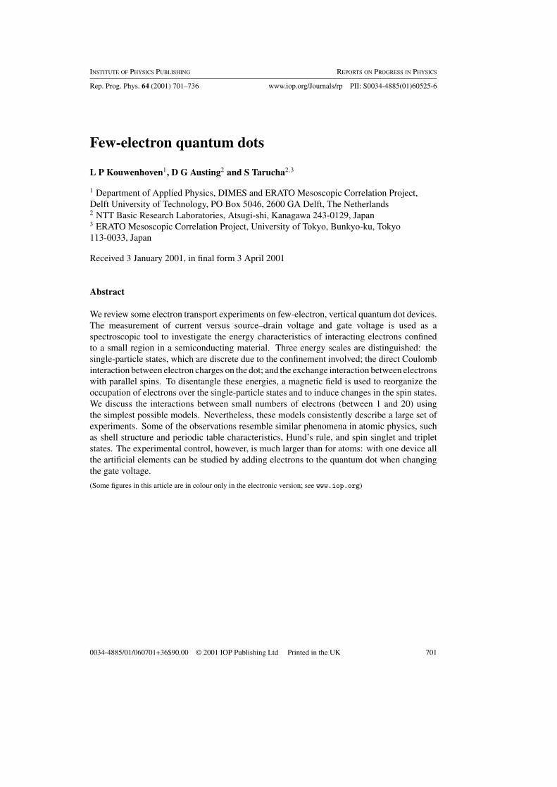
Capacitance [42] and tunnelling [15] spectroscopy have provided evidence of STtransitions. Here, we review the results on our vertical circular dots [43, 44]. Figure 18shows the linear-response Coulomb-blockade peaks for N = 0–4 reflecting the GS evolutionwithB. We emphasize that, based on the Fock–Darwin spectrum for non-interacting electrons,
728 L P Kouwenhoven et al
one does not expect transitions or kinks in the B-dependence of µ(N) forN = 1–4. The peakfor N = 1 indeed has a smooth B-dependence. For N = 2, 3 and 4, however, we observekinks, which are indicated by arrows. These kinks must arise from interactions not includedin the CI model. (The left arrow in the N = 4 trace is due to the Hund’s rule state, whichwas discussed in section 4.2.) To focus on the difference between the N = 1 and 2 traces,we have extracted the peak positions and converted their values from gate voltage to energy.The two curves in figure 18(b) are shifted towards each other and represent the variation inthe electrochemical potential with B. The lowest curve for N = 1 shows a smooth increasein energy in accordance with the expected trend for E0,0. The N = 2 trace rises faster with Bthan theN = 1 curve. This reflects the magnetic-field dependent Coulomb interaction Ec(B).The expected ST transition in the two-electron GS is observed as a kink labelled ‘a’ at 4.5 T.A crossing between the GS and the first ES is observed clearly in the corresponding excitationstripe. In figure 18(c) a grey scale plot of I (Vg, B) is shown for the N = 2 stripe measuredfor Vsd = 4 mV. Within the stripe, the first ES first decreases with B similar to µ↑↑(2) (dottedcurve in figure 17). The ST crossing takes place at about 4.5 T. These measurements confirmthe idea that electron–electron interactions have a strong effect on spin transitions.
We briefly discuss the N = 3 and 4 curves in figure 18(a), which both contain two kinks.The left kink (labelled ‘b’) in µ(3) = U(3) − U(2) is not due to a transition in the energyU(3), but is a remnant of the two-electron ST transition in U(2). The right kink (labelled‘c’) corresponds to the transition from U(3) = E0,0(↑) + E0,0(↓) + E0,1(↑) + 3Ec to thespin-polarized case U(3) = E0,0(↑) + E0,1(↑) + E0,2(↑) + 3Ec. Detailed analysis also showsthat this transition to an increasing total angular momentum and total spin is driven largely byinteractions [43]. Similar transitions occur for theN = 4 system where on the right of the lastkink (labelled ‘e’) the system is again in a polarized state with sequential filling of the angularmomentum states: U(4) = E0,0(↑) + E0,1(↑) + E0,2(↑) + E0,3(↑) + 6Ec.
8. Experimental determination of direct Coulomb and exchange interactions
We discussed in section 4.2 how Hund’s rule accounts for the energy associated with spin fillingnear B = 0. For two electrons we have explicitly discussed how a magnetic field changesthe Coulomb interactions such that the system undergoes a ST transition. In this section wediscuss a simple, but general model that describes filling of two single-particle states with twointeracting electrons [27]. This model that generalizes Hund’s rule to arbitrary B-field [34],allows one to determine from experimental data on dots with larger electron numbers thecontributions from the direct and exchange interactions (see equation (6)).
Figure 19(a) shows two, spin-degenerate single-particle states with energies Ea and Ebcrossing each other at B = B0. The GS energy, U(1), for one electron occupying these states,equals Ea for B < B0 and Eb for B > B0 (thick curve in figure 19(a)). For two electrons wecan distinguish four possible configurations with either total spin S = 0 (spin-singlet) or S = 1(spin-triplet). (We neglect the Zeeman-energy difference between the z-component Sz = −1,0 and 1.) The corresponding energies, Ui(2, S) for i = 1–4, are given by
U1(2, 0) = 2Ea + Caa,
U2(2, 0) = 2Eb + Cbb,
U3(2, 1) = Ea + Eb + Cab − |Kab|, (note S = 1!)
U4(2, 0) = Ea + Eb + Cab.
As in equation (6), Cij (i, j = a, b) is the direct Coulomb energy between two electronsoccupying states with energies Ei and Ej , andKab is the exchange energy (Kab < 0) between
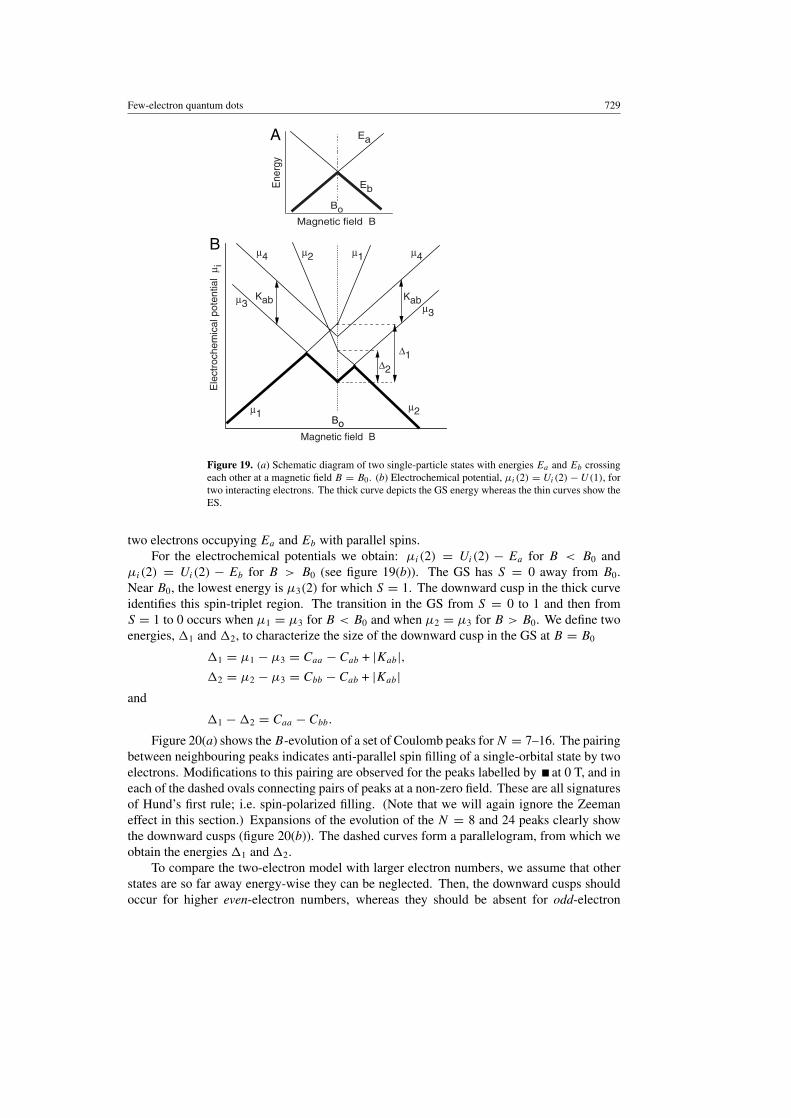
Few-electron quantum dots 729
B
Magnetic field B
Magnetic field B
Ea
Ene
rgy
Bo
∆1∆2
Bo
µ2
µ2
µ1
µ1
µ3µ3
Ele
ctro
chem
ical
pote
ntia
lµ i
Eb
µ4µ4
Kab Kab
A
Figure 19. (a) Schematic diagram of two single-particle states with energies Ea and Eb crossingeach other at a magnetic field B = B0. (b) Electrochemical potential, µi(2) = Ui(2)− U(1), fortwo interacting electrons. The thick curve depicts the GS energy whereas the thin curves show theES.
two electrons occupying Ea and Eb with parallel spins.For the electrochemical potentials we obtain: µi(2) = Ui(2) − Ea for B < B0 and
µi(2) = Ui(2) − Eb for B > B0 (see figure 19(b)). The GS has S = 0 away from B0.Near B0, the lowest energy is µ3(2) for which S = 1. The downward cusp in the thick curveidentifies this spin-triplet region. The transition in the GS from S = 0 to 1 and then fromS = 1 to 0 occurs when µ1 = µ3 for B < B0 and when µ2 = µ3 for B > B0. We define twoenergies, �1 and �2, to characterize the size of the downward cusp in the GS at B = B0
�1 = µ1 − µ3 = Caa − Cab + |Kab|,�2 = µ2 − µ3 = Cbb − Cab + |Kab|
and
�1 −�2 = Caa − Cbb.Figure 20(a) shows theB-evolution of a set of Coulomb peaks forN = 7–16. The pairing
between neighbouring peaks indicates anti-parallel spin filling of a single-orbital state by twoelectrons. Modifications to this pairing are observed for the peaks labelled by at 0 T, and ineach of the dashed ovals connecting pairs of peaks at a non-zero field. These are all signaturesof Hund’s first rule; i.e. spin-polarized filling. (Note that we will again ignore the Zeemaneffect in this section.) Expansions of the evolution of the N = 8 and 24 peaks clearly showthe downward cusps (figure 20(b)). The dashed curves form a parallelogram, from which weobtain the energies �1 and �2.
To compare the two-electron model with larger electron numbers, we assume that otherstates are so far away energy-wise they can be neglected. Then, the downward cusps shouldoccur for higher even-electron numbers, whereas they should be absent for odd-electron

730 L P Kouwenhoven et al
Figure 20. (a) Evolution of the GS energies for N = 7–16. The bars along the gate voltageaxis show 1 meV energy scales calibrated at −1.26 and −0.85 V. The dotted curve indicates thelast crossing between single-particle states. Dashed ovals correlate pairs of GSs for odd and evenelectron numbers. The spin transitions in the GSs are indicated by at B = 0 T and occur inthe ovals for B �= 0 T. (b) Magnified plots of the cusps for N = 8 and 24. The dashed curvesillustrate how the interaction-energy parameters, �1 and �2 are determined. (c) Fock–Darwinsingle-particle states calculated for hωo = 2 meV.
numbers. This is clearly observed in the ovals in figure 20(a). For instance, the B-fielddependence of the ninth peak compares well to the thick curve in figure 19(a) and the B-fielddependence of the tenth peak compares well to the thick curve in figure 19(b). Other pairsof even and odd numbered peaks show the same behaviour. This justifies our assumption ofsimplifying the many-electron system to just one or two electrons.
Figure 21 shows the excitation spectrum in a dI/dVg plot, taken for Vsd = 2 mV. As insection 5.2, this larger voltage opens a sufficiently wide transport window between the Fermilevels of the source and drain, that both the GS and first few ESs can be detected. The GS andES for N = 7–9 can be assigned from the magnetic-field dependence of the dark blue curves.The solid red curves highlight the GS whereas the dashed red curves indicate the ES. The setof the GS and ES curves for N = 7 shows a single crossing similar to that in figure 19(a).The spectrum for N = 8 compares well to figure 19(b) and we can clearly distinguish theparallelogram formed by the GS and first ES. The downward cusp in the GS for N = 8
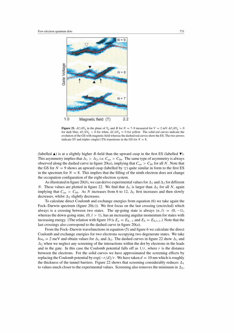
Few-electron quantum dots 731
Figure 21. dI/dVg in the plane of Vg and B for N = 7–9 measured for V = 2 mV. dI/dVg > 0for dark blue, dI/dVg < 0 for white, dI/dVg ≈ 0 for yellow. The solid red curves indicate theevolution of the GS with magnetic field whereas the dashed red curves show the ES. The two arrowsindicate ST and triplet–singlet (TS) transitions in the GS for N = 8.
(labelled �) is at a slightly higher B-field than the upward cusp in the first ES (labelled �).This asymmetry implies that�1 > �2, i.e.Caa > Cbb. The same type of asymmetry is alwaysobserved along the dashed curve in figure 20(a), implying that Caa > Cbb for all N . Note thatthe GS for N = 9 shows an upward cusp (labelled by �) quite similar in form to the first ESin the spectrum for N = 8. This implies that the filling of the ninth electron does not changethe occupation configuration of the eight-electron system.
As illustrated in figure 20(b), we can derive experimental values for�1 and�2 for differentN . These values are plotted in figure 22. We find that �1 is larger than �2 for all N , againimplying that Caa > Cbb. As N increases from 6 to 12, �1 first increases and then slowlydecreases, whilst �2 slightly decreases.
To calculate direct Coulomb and exchange energies from equation (6) we take again theFock–Darwin spectrum (figure 20(c)). We first focus on the last crossing (encircled) whichalways is a crossing between two states. The up-going state is always (n, l) = (0,−1),whereas the down-going state, (0, l > 1), has an increasing angular momentum for states withincreasing energy. (The relation with figure 19 is Ea = E0,−1 and Eb = E0,l>1.) Note that thelast crossings also correspond to the dashed curve in figure 20(a).
From the Fock–Darwin wavefunctions in equation (5) and figure 6 we calculate the directCoulomb and exchange energies for two electrons occupying two degenerate states. We takehωo = 2 meV and obtain values for �1 and �2. The dashed curves in figure 22 show �1 and�2 when we neglect any screening of the interactions within the dot by electrons in the leadsand in the gate. In this case the Coulomb potential falls off as 1/r , where r is the distancebetween the electrons. For the solid curves we have approximated the screening effects byreplacing the Coulomb potential by exp{−r/d}/r . We have taken d = 10 nm which is roughlythe thickness of the tunnel barriers. Figure 22 shows that screening considerably reduces �1
to values much closer to the experimental values. Screening also removes the minimum in�2,

732 L P Kouwenhoven et al
∆1 unscr)(
∆2(exp)
∆1(scr)
2(scr)
0.1
0.5
K (unscr)abK (scr)ab
∆2(unscr)
Electron number N
Ene
rgy
(meV
)
∆1(exp)
∆
Figure 22. Experimental values for the energy parameters�1 (•) and�2 ( ), on a log scale, versuselectron number derived from data as shown in figure 20(a). The uncertainty in the determinationof the experimental values is ±10% or less. The dashed and solid curves are calculated fromthe Fock–Darwin wavefunctions at 2 T, for an unscreened (unscr) and screened (scr) Coulombinteraction. The calculated exchange energy |Kab| between states with energies Ea = E0,−1 andEb = E0,N/2−1 decreases quickly with N .
which is in better agreement with the experimental values.Since the average radius of the wavefunctions increases with angular momentum, two
electrons are closer together when they both occupy (0,−1) compared to both occupying(0, l = N/2 − 1) for l > 1. The direct Coulomb interactions are thus stronger in the first case.This explains our observation �1 > �2, that is Caa > Cbb for all N. The overlap betweendifferent wavefunctions, (0,−1) and (0, l = N/2 − 1), decreases with N for l > 1. Thisresults in a decrease in both Cab and |Kab| with N . It then follows that �1 increases until itsaturates at a value equal to Caa . The gradual decrease of experimental �1 for N > 12 isprobably related to the decrease in the lateral confinement withN and thus the decrease inCaa .
Note that the asymmetry (�1 �= �2) can only occur for B0 �= 0. Symmetry is requiredif B0 = 0, implying that �1 = �2. Then, the eigenfunctions for the states with energyEa and Eb must have the same spatial form, so for general reasons we conclude that atB0 = 0 : Caa = Cbb = Cab and thus �1 = �2 = |Kab|. We can determine these energiesfor the N = 4, 8 and 14 peaks near B = 0 T (the N = 8 and 14 peaks are labelled infigure 20(a)). These peaks correspond to the GS electrochemical potentials for adding thesecond electron to the second, third and fourth shells, respectively. For these electron numberswe can simplify theN -electron system to a two-electron system that is well-separated in energyfrom the other N − 2 electron system. The inset to figure 23 demonstrates the resemblance to
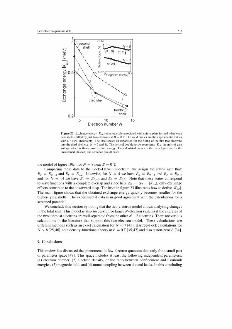
Few-electron quantum dots 733
0 0.7
Ga
te v
olta
ge
(V
)
(0, 2)
(0, 2)
(0, -2)
-1.29
-1.18
N = 8
N = 7
Magnetic field (T)
secondshell
third shell
fourth shell
Electron number N
1
0.2
0.5
Exc
ha
ng
e e
nerg
y K
(
meV
)a
b
Figure 23. Exchange energy |Kab| on a log scale associated with spin-triplets formed when eachnew shell is filled by just two electrons at B = 0 T. The solid circles are the experimental valueswith a ∼10% uncertainty. The inset shows an expansion for the filling of the first two electronsinto the third shell (i.e. N = 7 and 8). The vertical double-arrow represents |Kab| in units of gatevoltage which is then converted into energy. The calculated curves in the main figure are for theunscreened (dashed) and screened (solid) cases.
the model of figure 19(b) for N = 8 near B = 0 T.Comparing these data to the Fock–Darwin spectrum, we assign the states such that:
Ea = E0,−2 and Eb = E0,2. Likewise, for N = 4 we have Ea = E0,−1 and Eb = E0,1,and for N = 14 we have Ea = E0,−3 and Eb = E0,3. Note that these states correspondto wavefunctions with a complete overlap and since here �1 = �2 = |Kab|, only exchangeeffects contribute to the downward cusp. The inset in figure 23 illustrates how to derive |Kab|.The main figure shows that the obtained exchange energy quickly becomes smaller for thehigher-lying shells. The experimental data is in good agreement with the calculations for ascreened potential.
We conclude this section by noting that the two-electron model allows analysing changesin the total spin. This model is also successful for larger N -electron systems if the energies ofthe two topmost electrons are well separated from the otherN−2 electrons. There are variouscalculations in the literature that support this two-electron model. These calculations usedifferent methods such as an exact calculation for N < 7 [45], Hartree–Fock calculations forN > 8 [25,46], spin density-functional theory atB = 0 T [35,47] and also at non-zeroB [34].
9. Conclusions
This review has discussed the phenomena in few-electron quantum dots only for a small partof parameter space [48]. This space includes at least the following independent parameters:(1) electron number, (2) electron density, or the ratio between confinement and Coulombenergies, (3) magnetic field, and (4) tunnel coupling between dot and leads. In this concluding

734 L P Kouwenhoven et al
section we briefly discuss the different regimes one encounters along these different axes.
(1) Electron number. We have restricted this review to few-electron systems. For not toomany electrons the shell structure is regularly filled with electrons obeying general rules.The total energies can be discussed by bookkeeping the different contributions. Suchsimple models together with numerical calculations provide a thorough understanding. Incontrast, for large electron systems (∼50 < N < ∼1000) there are still many unansweredquestions. In these systems there is not usually a clear separation of the energy scales [6].The experimental status is that properties like an excitation spectrum on a particular devicelooks too complicated to comprehend in detail [29]. Alternatively, statistical theories havebeen applied to describe properties such as average energy spacings and their variance.However, this approach has also been unable to provide a consistent description of largerquantum dots [7].
(2) Electron density. For a fixed electron number the density varies with the confinementpotential. The two extremes on this axis are at one end a quantum regime (where confine-ment dominates and Coulomb interactions form a small perturbation) and at the other enda classical regime (where confinement is so weak that quantum fluctuations are absent).Our devices are somewhere in the middle. One interesting prediction is that in the classicalregime the correlations due to Coulomb interactions can become so strong that the elec-trons freeze to regular, fixed positions and form a Wigner lattice [49]. It is unclear how suchcorrelations can be observed unambiguously in transport experiments as in this review.
(3) Magnetic field. This review covers only moderate magnetic fields, mostly for ωc < ωo.We have used the magnetic field to induce transitions between single-particle states orspin states. However, the ‘type of states’ did not change. For larger magnetic fields,ωc > ωo, one enters the regimes of the integer and fractional quantum Hall effect. Here,many-body states can arise such as skyrmions or excitations with a fractional charge. Onfew-electron, vertical quantum dots, some high B-field experiments have been performedin the integer quantum Hall regime, probing spin flips on decreasing the filling factor from2 to 1 [18,19,50], and the stability of the maximum-density droplet [51]. To date, no clearresults have been obtained in the fractional regime.
(4) Tunnel coupling between dot and leads. We have only discussed the regime of weak tunnelcoupling; i.e. for tunnel resistances much larger than e2/h = 25 k%. In this regime the timethat an electron spends on the dot is assumed to be much larger than typical relaxation times,implying that the system always returns to equilibrium between consecutive tunnellingevents. In addition, the tunnel rate, or lifetime broadening, 2, has been neglected since inthe experiments in this review it has always been much smaller than the thermal energy,kBT . Devices have also been made with thinner tunnel barriers so that 2 kBT . In thesedevices the Coulomb blockade is no longer complete and higher-order tunnelling processesbecome visible [52]. Such so-called co-tunnelling events can give rise to the Kondoeffect, a many-body effect where many electrons together screen the localized spin on thequantum dot [53]. Under these circumstances quantum dots play a similar role as magneticimpurities in metals, however, again with a much higher degree of experimental control.
The study of transport through few-electron quantum dots was until recently impossiblein lateral quantum dots defined by surface gates in a two-dimensional electron gas. However,recently Ciorga et al and Gould et al [54] realized the few-electron limit in lateral dots.This opens up exciting combinations of experiments on lateral dots (applying high-frequencysignals, putting dots in rings, etc [6]) with few-electron regimes where the quantum states arewell understood.
Few-electron quantum dots 735
Acknowledgments
The authors would like to thank in particular all the collaborators listed in the periodic tableof acknowledgements in figure 2. They further acknowledge the financial support from theSpecially Promoted Research, Grant-in-Aid for Scientific Research, from the Ministry ofEducation, Science and Culture in Japan, from the Dutch Organization for FOM, from theNEDO program NTDP-98, and from the EU via a TMR network.
References
[1] See for reviews in popular magazines: Reed M 1993 Sci. Am. 268 118Kastner M A 1993 Phys. Today 46 24Ashoori R C 1996 Nature 379 413Harmans C J P M 1992 Phys. World 5 50Kouwenhoven L P and Marcus C M 1998 Phys. World 11
[2] Alonso M and Finn E J 1968 Quantum and Statistical Physics (Reading, MA: Addison-Wesley)[3] Austing D G, Honda T, Tokura Y and Tarucha S 1995 Japan. J. Appl. Phys. 34 1320
Austing D G, Honda T and Tarucha S 1996 Semicond. Sci. Technol. 11 388[4] Tarucha S, Austing D G, Honda T, van der Hage R J and Kouwenhoven L P 1996 Phys. Rev. Lett. 77 3613[5] Keren K, Stern A and Sivan U 1999 Preprint cond-mat/9903377[6] See for a review on quantum dots: Kouwenhoven L P, Marcus C M, McEuen P L, Tarucha S, Westervelt R M
and Wingreen N S 1997 Electron transport in quantum dots Mesoscopic Electron Transport ed L L Sohn,G Schon and L P Kouwenhoven (Kluwer Series E vol 345) (June 1996) p 105–214 see also: webpagehttp://vortex.tn.tudelft.nl/
[7] Marcus C M, Patel S R, Huibers A G, Cronenwett S M, Switkes M, Chan I H, Clarke R M, Folk J A andGodijn S F 1997 Chaos Solitons Fractals 8 1261
[8] Ralph D C, Black C T, Hergenrother J M, Lu J G and Tinkham M 1997 Mesoscopic Electron Transport edL L Sohn, L P Kouwenhoven and G Schon (Kluwer Series E vol 345) (June 1996) p 447–67
[9] Dekker C 1999 Phys. Today May[10] Grabert H and Devoret M H (ed) 1991 Single Charge Tunnelling (New York: Plenum)
Jacak L’, Harylak P and Wojs A 1998 Quantum Dots (Berlin: Springer)[11] Iafrate G J, Hess K, Krieger J B and Macucci M 1995 Phys. Rev. B 52 10737[12] Hadley P and Mooij J E 2000 Quantum Semiconductor Devices and Technologies ed T P Pearsall (Dordrecht:
Kluwer)[13] Mizuto H and Tanoue T 1996 The Physics and Applications of Resonant Tunnelling Diodes (Cambridge:
Cambridge University Press)[14] Tokura Y 1999 Private communication[15] Su B, Goldman V J and Cunningham J E 1992 Phys. Rev. B 46 7644
Tewordt M, Martın-Moreno L, Law V J, Kelly M J, Newbury R, Pepper M, Ritchie D A, Frost J E F andJones G A C 1992 Phys. Rev. B 46 3948
Schmidt T, Tewordt M, Blick R H, Haug R J, Pfannkuche D, von Klitzing K, Forster A and Luth H 1995 Phys.Rev. B 51 5570
[16] Dellow M W, Beton P H, Langerak C J G M, Foster T J, Main P C, Eaves L, Henini M, Beaumont S P andWilkinson C D W 1992 Phys. Rev. Lett. 68 1754
Gueret P, Blanc N, Germann R and Rothuizen H 1992 Phys. Rev. Lett. 68 1896[17] Tarucha S, Austing D G and Honda T 1995 Superlatt. Microstruct. 18 121[18] Ashoori R C, Stormer H L, Weiner J S, Pfeiffer L N, Pearton S J, Baldwin K W and West K W 1992 Phys. Rev.
Lett. 68 3088[19] Ashoori R C, Stormer H L, Weiner J S, Pfeiffer L N, Baldwin K W and West K W 1993 Phys. Rev. Lett. 71 613[20] Korotkov A N, Averin D V and Likharev K K 1990 Physica B 165/166 927
Beenakker C W J 1991 Phys. Rev. B 44 1646Averin D V, Korotkov A N and Likharev K K 1991 Phys. Rev. B 44 6199
[21] Fock V 1928 Z. Phys. 47 446Darwin C G 1930 Proc. Camb. Phil. Soc. 27 86
[22] Halonen V, Hyvonen P, Pietilinen P and Chakraborty T 1996 Phys. Rev. B 53 6971[23] Macucci M, Hess K and Iafrate G J 1993 Phys. Rev. B 48 17354
Macucci M, Hess K and Iafrate G J 1995 J. Appl. Phys. 77 3267

736 L P Kouwenhoven et al
[24] Zeng Y H, Goodman B and Serota R A 1993 Phys. Rev. B 47 15660[25] Rontani M, Rossi F, Manghi F and Molinari E 1997 Appl. Phys. Lett. 72 975
Rontani M, Rossi F, Manghi F and Molinari E 1999 Phys. Rev. B 59 10165[26] Warburton R J, Miller B T, Durr C S, Bodefeld C, Karrai K, Kotthaus J P, Medeiros-Ribeiro G and Petroff P M
1998 Phys. Rev. B 58 16221[27] Tarucha S, Austing D G, Tokura Y, van der Wiel W G and Kouwenhoven L P 2000 Phys. Rev. Lett. 84 2485[28] Stopa M 1996 Phys. Rev. B 54 13767[29] Stewart D R, Sprinzak D, Marcus C M, Duruoz C I and Harris J S 1997 Science 278 1784[30] Heiss W D and Nazmitdinov R G 1996 Phys. Lett. A 222 309[31] Ezaki T, Mori N and Hamaguchi C 1997 Phys. Rev. B 56 6428[32] Angelucci A and Tagliacozzo A 1997 Phys. Rev. B 56 7088[33] Nagaraja S, Matagne P, Thean V-Y, Leburton J-P, Kim Y-H and Martin R M 1997 Phys. Rev. B 56 15752[34] Steffens O, Rossler U and Suhrke M 1998 Europhys. Lett. 42 529[35] Lee I-H, Rao V, Martin R M and Leburton J-P 1998 Phys. Rev. B 57 9035[36] Harting J, Mulken O and Borrmann P 2000 Phys. Rev. B 62 10207–11[37] Wojs A and Hawrlylak P 1996 Phys. Rev. B 53 10841[38] See, for example, Kumar A, Laux S E and Stern F 1990 Phys. Rev. B 42 5166–75
Hallam L D, Weis J and Maksym P A 1996 Phys. Rev. B 53 1452[39] Bednarek S, Szafran B and Adamowski J 2000 Phys. Rev. B 61 4461[40] Wagner M, Merkt U and Chaplik A V 1992 Phys. Rev. B 45 1951[41] Thurner G, Herold H, Ruder H, Schlicht G and Wunner G 1982 Phys. Lett. A 89 133[42] Ashoori R C, Stormer H L, Weiner J S, Pfeiffer L N, Baldwin K W and West K W 1993 Phys. Rev. Lett. 71 613[43] Kouwenhoven L P, Oosterkamp T H, Danoesastro M W S, Eto M, Austing D G, Honda T and Tarucha S 1997
Science 278 1788[44] van der Wiel W G, Oosterkamp T H, Janssen J W, Kouwenhoven L P, Austing D G, Honda T and Tarucha S
1998 Physica B 256–8 173[45] Eto M 1997 Japan. J. Appl. Phys. 36 3924[46] Natori A et al 1997 Japan. J. Appl. Phys. 36 3960
Tamura H 1998 Physica B 249–51 210Hirose K and Wingreen N S 1999 Phys. Rev. B 59 4604–7
[47] Koskinen M, Manninen M and Reimann S M 1997 Phys. Rev. Lett. 79 1817[48] See also our review that includes a discussion on the effects of symmetry-breaking in non-circular quantum dots:
Tarucha S, Austing D G, Sasaki S, Tokura Y, van der Wiel W G and Kouwenhoven L P 2000 Appl. Phys. A71 367–78
[49] Bryant G W 1987 Phys. Rev. Lett. 59 1140Hausler W, Kramer B and Masek J 1991 Z. Phys. B 85 435Maksym P A 1993 Physica B 184 385Bedanov V M and Peeters F M 1994 Phys. Rev. B 49 2667Koulakov A A and Scklovskii B I 1998 Phys. Rev. B 57 2352–67
[50] Austing D G, Tokura Y, Honda T, Tarucha S, Danoesastro M, Janssen J W, Oosterkamp T H and Kouwenhoven L P1999 Japan. J. Appl. Phys. 38 372–5
[51] Oosterkamp T H, Janssen J W, Kouwenhoven L P, Austing D G, Honda T and Tarucha S 1999 Phys. Rev. Lett.82 2931–4
[52] De Franceschi S, Sasaki S, Elzerman J M, van der Wiel W G, Tarucha S and Kouwenhoven L P 2001 Phys. Rev.Lett. 86 878–81
[53] Sasaki S, De Franceschi S, Elzerman J M, van der Wiel W G, Eto M, Tarucha S and Kouwenhoven L P 2000Nature 405 764–7
[54] Ciorga M, Sachrajda A S, Hawrylak P, Gould C, Zawadzki P, Jullian S, Feng Y and Wasilewski Z 2000 Phys.Rev. B 61 R16315–8
Gould C, Hawrylak P, Sachrajda A, Feng Y, Zawadzki P and Wasilewski Z 2000 Physica E 6 461–5
Related Documents