Feshbach Resonances in 40 K Antje Ludewig

Welcome message from author
This document is posted to help you gain knowledge. Please leave a comment to let me know what you think about it! Share it to your friends and learn new things together.
Transcript

Feshbach Resonances in 40K
Antje Ludewig

Feshbach Resonances in 40K
Academisch Proefschrift
ter verkrijging van de graad van doctor
aan de Universiteit van Amsterdam
op gezag van de Rector Magnificus prof. dr. D.C. van den Boom
ten overstaan van een door het college voor promoties ingestelde
commissie, in het openbaar te verdedigen in de Agnietenkapel
op vrijdag 16 maart 2012, te 12:00 uur
door
Antje Ludewig
geboren te Reutlingen, Duitsland
Promotiecommissie:
Promotor: prof. dr. J.T.M. Walraven
Overige leden: prof. dr. M.S. Goldendr. T.W. Hijmansdr. ir. S.J.J.M.F. Kokkelmansprof. dr. H.B. van Linden van den Heuvellprof. dr. G.V. Shlyapnikovprof. dr. C. Zimmermann
Faculteit der Natuurwetenschappen, Wiskunde en Informatica (FNWI)
ISBN: 978-94-6191-188-9
Cover showing loss features around Feshbach resonances in the d + e mixture in theclouds above Noetzie beach, photo by the author, design and implementation by BodoLudewig.
The work described in this thesis was carried out in the group "Quantum Gases andQuantum Information" at the Van der Waals–Zeeman Institute of the University ofAmsterdam, Science Park 904, 1098 XH Amsterdam, The Netherlands. A limitednumber of hard copies of this thesis is available there.A digital version of this thesis including the hyperlinks to the cited articles can bedownloaded fromhttp://www.science.uva.nl/~walraven or http://dare.uva.nl .This work is part of the research programme of the Foundation for Fundamental Re-search on Matter (FOM), which is part of the Netherlands Organisationfor Scientific Research (NWO).
Contents
1 Introduction 11.1 Cold quantum gases . . . . . . . . . . . . . . . . . . . . . . . . . . . . 21.2 This thesis . . . . . . . . . . . . . . . . . . . . . . . . . . . . . . . . . . 31.3 Outline . . . . . . . . . . . . . . . . . . . . . . . . . . . . . . . . . . . . 3
2 Theoretical Background 52.1 Fermions . . . . . . . . . . . . . . . . . . . . . . . . . . . . . . . . . . . 52.2 Two-body Hamiltonian . . . . . . . . . . . . . . . . . . . . . . . . . . . 6
2.2.1 Internal Hamiltonian . . . . . . . . . . . . . . . . . . . . . . . . 72.2.2 Hamiltonian for the relative motion . . . . . . . . . . . . . . . . 8
2.3 Elastic collisions . . . . . . . . . . . . . . . . . . . . . . . . . . . . . . . 92.4 Spin Exchange and 40K . . . . . . . . . . . . . . . . . . . . . . . . . . . 10
2.4.1 Populated states in the magnetic trap . . . . . . . . . . . . . . . 132.4.2 Scattering rate for spin exchange . . . . . . . . . . . . . . . . . 13
2.5 Feshbach resonances . . . . . . . . . . . . . . . . . . . . . . . . . . . . 142.6 Asymptotic bound state model . . . . . . . . . . . . . . . . . . . . . . 162.7 Trapped fermions . . . . . . . . . . . . . . . . . . . . . . . . . . . . . . 17
2.7.1 Fermi degenerate density distribution . . . . . . . . . . . . . . . 18
3 Experimental setup 213.1 Introduction . . . . . . . . . . . . . . . . . . . . . . . . . . . . . . . . . 213.2 Vacuum system . . . . . . . . . . . . . . . . . . . . . . . . . . . . . . . 223.3 Laser system . . . . . . . . . . . . . . . . . . . . . . . . . . . . . . . . 253.4 Magneto-optical trapping . . . . . . . . . . . . . . . . . . . . . . . . . . 28
3.4.1 Two-dimensional MOT for 40K . . . . . . . . . . . . . . . . . . . 283.4.2 Three-dimensional MOT . . . . . . . . . . . . . . . . . . . . . . 30
3.5 Optically plugged magnetic trap . . . . . . . . . . . . . . . . . . . . . . 313.5.1 Magnetic trap . . . . . . . . . . . . . . . . . . . . . . . . . . . . 323.5.2 Optical plug . . . . . . . . . . . . . . . . . . . . . . . . . . . . . 34
3.6 Optical dipole trap . . . . . . . . . . . . . . . . . . . . . . . . . . . . . 353.6.1 Intensity stabilization of the fibre laser . . . . . . . . . . . . . . 36
3.7 Feshbach coils . . . . . . . . . . . . . . . . . . . . . . . . . . . . . . . . 383.8 Imaging systems . . . . . . . . . . . . . . . . . . . . . . . . . . . . . . 41
3.8.1 Cameras and optical setup . . . . . . . . . . . . . . . . . . . . . 413.8.2 Fluorescence imaging . . . . . . . . . . . . . . . . . . . . . . . . 433.8.3 Absorption imaging . . . . . . . . . . . . . . . . . . . . . . . . . 43
vi Contents
3.8.4 High-field imaging . . . . . . . . . . . . . . . . . . . . . . . . . 443.9 Computer control and analysis . . . . . . . . . . . . . . . . . . . . . . . 47
3.9.1 Control program and hardware . . . . . . . . . . . . . . . . . . 473.9.2 Software . . . . . . . . . . . . . . . . . . . . . . . . . . . . . . . 48
3.10 Sources for radio and microwave frequency . . . . . . . . . . . . . . . . 483.10.1 DDS systems . . . . . . . . . . . . . . . . . . . . . . . . . . . . 493.10.2 Amplification and switching . . . . . . . . . . . . . . . . . . . . 49
4 Experimental sequence 514.1 Atom cooling and trapping . . . . . . . . . . . . . . . . . . . . . . . . . 534.2 State preparation . . . . . . . . . . . . . . . . . . . . . . . . . . . . . . 55
4.2.1 State cleaning . . . . . . . . . . . . . . . . . . . . . . . . . . . . 564.2.2 State transfers . . . . . . . . . . . . . . . . . . . . . . . . . . . . 57
4.3 Field-dependent loss measurements . . . . . . . . . . . . . . . . . . . . 584.4 Stern-Gerlach imaging . . . . . . . . . . . . . . . . . . . . . . . . . . . 594.5 Magnetic field calibration . . . . . . . . . . . . . . . . . . . . . . . . . 594.6 Measured Feshbach resonances . . . . . . . . . . . . . . . . . . . . . . . 62
4.6.1 p-wave resonances with special features . . . . . . . . . . . . . . 634.6.2 Width of a Feshbach resonance . . . . . . . . . . . . . . . . . . 64
5 Feshbach resonances in 40K 695.1 Introduction . . . . . . . . . . . . . . . . . . . . . . . . . . . . . . . . . 695.2 Experiments . . . . . . . . . . . . . . . . . . . . . . . . . . . . . . . . . 71
5.2.1 Experiments in Amsterdam . . . . . . . . . . . . . . . . . . . . 735.2.2 Experiments in Munich . . . . . . . . . . . . . . . . . . . . . . . 755.2.3 Experiments in Zurich . . . . . . . . . . . . . . . . . . . . . . . 75
5.3 Theoretical models . . . . . . . . . . . . . . . . . . . . . . . . . . . . . 785.3.1 Coupled channels calculations . . . . . . . . . . . . . . . . . . . 785.3.2 Multichannel quantum defect theory . . . . . . . . . . . . . . . 835.3.3 Asymptotic bound state model . . . . . . . . . . . . . . . . . . 835.3.4 Comparison of MQDT and ABM . . . . . . . . . . . . . . . . . 85
5.4 Summary and conclusions . . . . . . . . . . . . . . . . . . . . . . . . . 87
AAtoms in optical potentials 89A.1 Optical potential for 40K . . . . . . . . . . . . . . . . . . . . . . . . . . 89A.2 Rotating wave approximation . . . . . . . . . . . . . . . . . . . . . . . 90A.3 Potential produced by a Gaussian beam . . . . . . . . . . . . . . . . . 91A.4 Density distribution . . . . . . . . . . . . . . . . . . . . . . . . . . . . . 92
A.4.1 Density in a harmonic potential . . . . . . . . . . . . . . . . . . 92A.4.2 Density in a Gaussian potential . . . . . . . . . . . . . . . . . . 92
BHyperfine structure 93B.1 Hyperfine splitting with an external magnetic field . . . . . . . . . . . 94B.2 Limit of high and low magnetic fields . . . . . . . . . . . . . . . . . . . 95B.3 Magnetic trapping potential . . . . . . . . . . . . . . . . . . . . . . . . 96
COptical transition probabilities 99C.1 Transition probabilities at zero magnetic field . . . . . . . . . . . . . . 99

Contents vii
C.2 Transition probabilities at non-zero magnetic field . . . . . . . . . . . . 100
Bibliography 105
Summary 119
Samenvatting 121
Acknowledgements 123
List of publications 127

Chapter 1
Introduction
Everyday we encounter the results of discoveries and achievements of quantum mechan-ics and atomic physics which were made over the last century: be it the laser diode ina DVD player displaying our holiday pictures or measurements of the thickness of theEarth’s ozone layer protecting us from UV radiation [Ste11]. In the first experimentsin atomic physics the structure of atoms and their unique absorption spectra weredeciphered, this is now the basis for thousands of applications from determining thevelocity at which the universe expands to measuring the alcohol content in the breathof a speeding driver.
Nowadays, using light and electro-magnetic fields, atoms can be manipulated andcooled to temperatures within a few 100 nK of absolute zero. At such low temperaturethe behaviour of the atoms is not determined by their external degrees of freedom, butby quantum statistics. Bosons, particles with integer spin, can condense into a singlestate and form a macroscopic wavefunction extending over the inter-particle distance.More than 70 years after the initial description by Bose and Einstein [Bos24, Ein25],these Bose-Einstein condensates (BEC) were demonstrated in atomic gases [And95,Dav95a] and recently light, the most prominent member in the class of bosons, wascondensed [Kla10].
For particles with half-integer spin, fermions, the behaviour at low temperaturesis very different from bosons: instead of lumping together they each occupy a stateby themselves, keeping their distance. The first degenerate quantum gas of fermionicatoms was produced in 40K [DeM99a]. The quantum statistics of fermions [Fer24,Fer26, Dir26] plays an important role in many areas of physics. In condensed matterFermi statistics determines electric and transport properties, neutron stars are pre-vented from collapsing by Fermi pressure and all matter known to us is composed ofquarks and electrons which are fermionic elementary particles. For the understandingof superconductivity the pairing of fermions with attractive interactions plays a majorrole [Che05]. Finding accurate theoretical descriptions for these phenomena and un-derstanding the influence of interactions and the quantum statistics of fermions is stillongoing work.
2 1. Introduction
1.1 Cold quantum gases
In cold quantum gases formed by neutral atoms there are no effects of electric chargeand crystal impurities and these systems enable us to observe the quantum nature ofparticles. Quantum degenerate gases have been used to demonstrate effects known fromcondensed matter physics, such as the Mott insulator - superfluid transition [Gre02,Jör08], the pairing of fermions [Reg04, Zwi05] and Anderson localization [Bil08, Roa08].A step further is to use systems of cold atoms as a simulator for other systems inphysics which are difficult or impossible to compute classically [Fey82]. This requiresthe implementation of controllable logic operations and a correlation of the atoms.
Strong correlations in experiments with cold quantum gases can be created eitherby confining the atoms tightly in optical lattices [Deu98, Gre02] or by tuning theinteraction between the atoms in strength and even sign with the help of so-calledFeshbach resonances [Fes58, Fes62, Chi10]. In cold atoms Feshbach resonances occurwhen a bound state within a two-body potential is resonant with the energy of a pairof unbound atoms. When the magnetic moments of the bound state and the unboundpair differs, they can be brought into resonance by applying a magnetic field. At theresonance, the scattering length, a measure for the interaction strength between atoms,diverges and changes sign.
The beauty and importance of Feshbach resonances is that they make it possible touse ultracold atoms as a model system for other areas of physics. Once the interactionbetween the atoms is strong enough, only a few universal parameters are required todescribe the system. Systems with entirely different underlying processes can then bestudied and compared to the strongly interacting cold atoms. At strong interactions thedescription of the cold atoms by mean-field theory breaks down and new methods needto be used. With the bosonic isotope of 39K it has been shown recently that dependingon the interaction strength the critical temperature for Bose-Einstein condensationchanges [Smi11].
For certain interaction strengths atoms can also form few-body bound states [Kra06]with universal properties described by Efimov [Efi70]. Although these states exist dueto two-body interaction, they are not present as two-body states. Efimov states arealso relevant in nuclear physics [Ham10].
With a Feshbach resonance the interaction in fermionic quantum gas can be tunedfrom repulsive to attractive through the so-called BEC-BCS crossover. A bosonicmolecule formed by two fermions can then transform into a pair of fermions coupled inmomentum space, similar to a Cooper pair in superconducting theory [Gio08, Ing07,Blo08]. With 40K this crossover has been explored [Ste08] and the condensation of thecomposite bosonic molecules into a BEC has been achieved [Gre03].
The positions and widths of Feshbach resonances of an atomic species in a specificstate depend on the interatomic potential, which differs for the different species andthe different states. Before Feshbach resonances can be used as a tool to tune theinteraction, their positions and properties need to be determined. The atomic specieswe are working with is 40K. It has been used as a single species [DeM99a, Lof02, Gre03]and others, but also in combination with the fermionic 6Li [Wil08, Tie10b, Nai11,Wu11], and the bosonic 87Rb [Sim03, Ino04, Fer06, Osp06a, Zir08a].
1.2. This thesis 3
1.2 This thesis
Feshbach resonances occur in a multitude, especially with a element like 40K, wheremany combinations of hyperfine states are stable. Prior to the results presented in thisthesis the position of four Feshbach resonances in mixtures of 40K in the three lowesthyperfine states was determined [Lof02, Reg03a, Reg03c, Reg06, Gae07]. In this thesiswe present measurements on mixtures occupying states in the middle of the hyperfinemanifold of 40K.
Relying on experiment alone, one can get lost in the large number of loss featuresas if wandering in the wilderness bearing neither map nor compass. To find ones wayin the uncharted area of Feshbach resonances it is necessary to start mapping outthe surroundings by starting at a known situation and not just wander off randomlyinto the terrain. All explorations in experiments have to go hand in hand with thetheoretical description of the position and nature of the resonance features.
With detailed knowledge of the interatomic potentials, the positions and propertiesof Feshbach resonances can be calculated using the coupled channel method (CC). How-ever, this method is computationally intensive and whether all resonances are founddepends on the step size in the numerical calculation. To predict the positions of newFeshbach resonances in previously unstudied state mixtures and to locate resonancesof special interest we use a simple asymptotic bound state model (ABM). Once exper-imental data is obtained the initial parameters of the ABM are improved and moreprecise predictions are calculated. The experimental data obtained is compared withanother approximate model, the multi quantum defect theory (MQDT), and the CCcalculations.
To reach temperatures cold enough to study the quantum nature and control theinteraction of the atoms, we use the techniques of laser cooling and evaporative cooling[Met99, Ket99]. We constructed an apparatus to cool and capture 40K and measureFeshbach resonances at a stable magnetic field. To investigate a Feshbach resonancein a certain channel it is of great importance to prepare the hyperfine state mixturesrequired in a reliable and reproducible manner, especially in the case of 40K with itsrich hyperfine structure. Without this, difficulties arise when assigning experimen-tally observed loss features. To achieve this we developed a state-dependent detectionscheme and a transfer procedure to populate the desired states. For the mapping outof Feshbach resonances we start out with binary mixtures of hyperfine states and mea-sure atom loss depending on the magnetic field. In a second step, the states can bemeasured individually to rule out p-wave resonances within one hyperfine state.
1.3 OutlineThis thesis covers both experimental and theoretical aspects of the study of Feshbachresonances in 40K. Chapter 2 contains a brief overview of the theoretical conceptsrequired to describe cold trapped fermions. The scattering of cold fermions and thetheory of Feshbach resonances are introduced. Here we put emphasis on the specifics of40K, which offers more options for stable state mixtures than other alkalis. Additionallythe simple model which we use to calculate the positions of Feshbach resonances ispresented.
4 1. Introduction
The major part of this thesis was to construct an apparatus to produce cold mix-tures of 6Li and 40K. In Chapter 3 this experimental apparatus is described, puttingthe emphasis on the 40K part and newly added components. Special features of ourapparatus include the two-dimensional magneto-optical traps used as sources for thecold atoms, an optically plugged magnetic trap and a transport of the cold atom cloudby means of optical tweezers.
The detailed experimental sequence to produce cold mixtures of specific states in40K is explained in Chapter 4. The calibration of the magnetic field is of importancefor the accurate specification of the measured data. How and to what precision wedetermine the magnetic field is also presented in Chapter 4. In this chapter we alsopresent measurements of Feshbach resonances which show special features. An indica-tion of the width of a Feshbach resonance is determined by evaporating the cold atomcloud at different magnetic fields; in Chapter 4 a model to fit the data is developed.
The main result of this thesis, the measurement of Feshbach resonances in variousspin mixtures of 40K, is presented in Chapter 5. The measured values are comparedwith values obtained by our collaborators in coupled channel calculations and the twosimple models. Overall we measured the position of 23 Feshbach resonances in elevendifferent state combinations.
The appendices cover more details about 40K in optical potentials (Appendix A),the hyperfine structure of 40K (Appendix B) and its optical transition probabilities(Appendix C).
Chapter 2
Theoretical Background
In this chapter the theoretical concepts and notations used in this thesis are presented.This chapter gives an overview of scattering theory and Feshbach resonances and theirdescription. We present the simplified model which was used to calculate the positionsof Feshbach resonances in 40K. This chapter also presents the assumptions to analyseand model the behaviour of ultracold atoms in external potentials. We put emphasison the peculiarities of 40K and the nature of fermions.
Cold quantum gases have a density which is in general low enough to describe theinteractions as two-body interactions. For low enough temperatures the descriptionof scattering processes by s-wave interaction is sufficient. The field of cold atoms isvery active and there are plenty of good textbooks and overview articles dealing withboth the theoretical aspects and the experimental techniques involved, for example[Ing07, Met99, Ket99, Chi05].
2.1 FermionsIn the everyday world as we experience it, two identical particles are never truly in-distinguishable. For example the movement and the trajectory of two billiard ballswhich look alike can be followed and backtracked either by eye or with the help of afast camera. Additionally two otherwise identical billiard balls can be marked withdifferent numbers and made distinguishable.
In quantum mechanics however, identical particles are truly indistinguishable. Theparticles can be specified by nothing more than a complete set of commuting observ-ables. According to the Heisenberg uncertainty principle it is not possible to obtainan exact measurement of all the observables simultaneously. The particles cannot belabelled and followed individually as in classical mechanics. When measuring a two-particle system of indistinguishable particles in state |ka〉 and state |kb〉, where the |ki〉represent a collective index for the complete set of observables, all linear combinationsof the two particles of the form
c1 |ka〉 |kb〉+ c2 |kb〉 |ka〉
result in identical eigenvalues. The eigenvalues are degenerate with respect to theexchange of the two particles |ka〉 and |kb〉, so at this level of analysis the linear com-
6 2. Theoretical Background
bination to describe the pair is not uniquely defined yet. This exchange degeneracyis lifted by including the exchange of two particles with the permutation operator P12with
P12 |ka〉 |kb〉 = |kb〉 |ka〉 .
Its eigenvalues are +1 and -1, so the description of a two-body system is either sym-metric or antisymmetric. It can be shown that in three dimensions the operator P12 isa constant of motion, as it commutes with the Hamiltonian [Sak94]. Being a constantof motion also implies that the symmetric and the antisymmetric solutions cannot beconverted into each other. Those two distinct solutions represent two distinct kindsof particles: bosons and fermions. Including the exchange of two particles, the non-degenerate solutions for the two-body wavefunction for two indistinguishable particlesa and b at positions r1 and r2 in terms of the single-particle wavefunctions ψi(ri) are:
ψ+(r1, r2) = CN (ψa(r1)ψb(r2) + ψb(r1)ψa(r2))ψ−(r1, r2) = CN (ψa(r1)ψb(r2)− ψb(r1)ψa(r2)), (2.1)
with a normalizing factor CN . Under exchange of the two particles the wavefunctionis symmetric for the plus-sign and antisymmetric for the minus-sign. The symmetricwavefunction is applicable for bosons and the antisymmetric version describes fermions.From Eq. 2.1 the Pauli exclusion principle [Pau25] becomes clear: two identical fermionscan neither occupy the same state ψi nor the same position r. For ψa = ψb the two-body wavefunction ψ−(r1, r2) vanishes, the same happens for r1 = r2. Particles witha half-integer spin, the fermions, obey Fermi-Dirac statistics [Dir26, Fer26], whereasparticles with integer spin, the bosons, obey Bose-Einstein statistics [Bos24, Ein25].For an ensemble of particles, the average number of particles ni per single particle stateεi is given by
nBEi = 1
e(εi−µ)/kBT − 1 (2.2)
for bosons andnFDi = 1
e(εi−µ)/kBT + 1 (2.3)
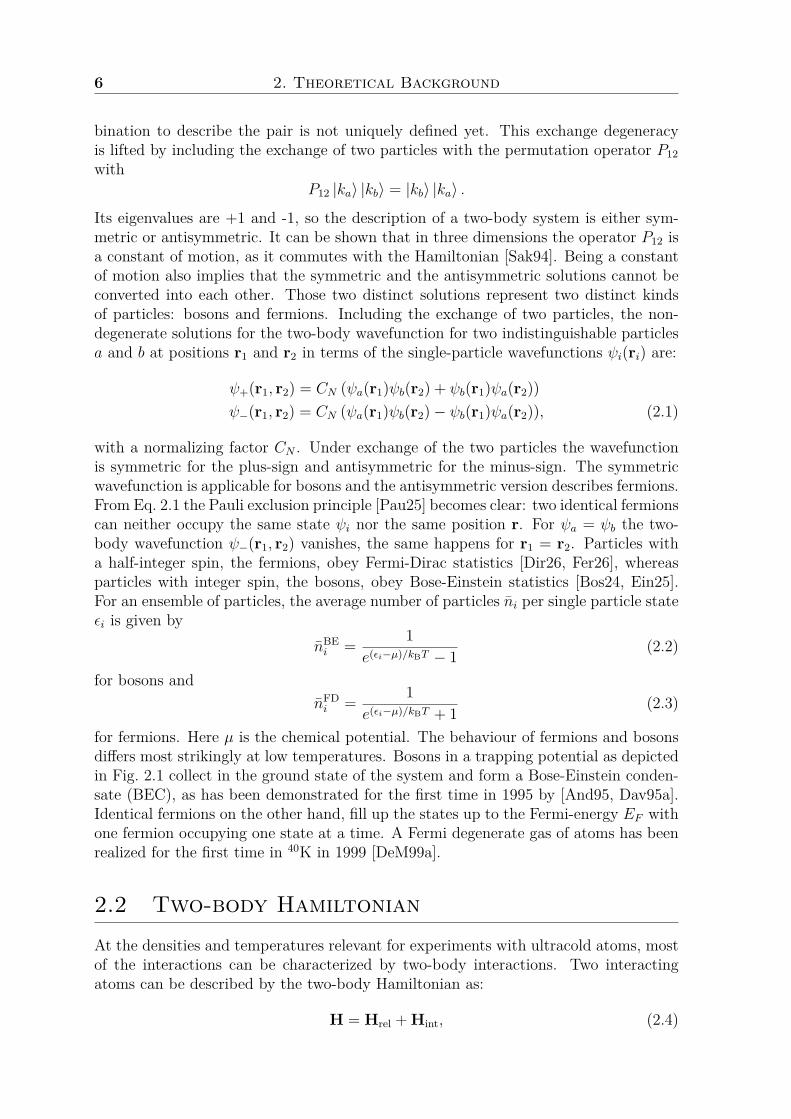
for fermions. Here µ is the chemical potential. The behaviour of fermions and bosonsdiffers most strikingly at low temperatures. Bosons in a trapping potential as depictedin Fig. 2.1 collect in the ground state of the system and form a Bose-Einstein conden-sate (BEC), as has been demonstrated for the first time in 1995 by [And95, Dav95a].Identical fermions on the other hand, fill up the states up to the Fermi-energy EF withone fermion occupying one state at a time. A Fermi degenerate gas of atoms has beenrealized for the first time in 40K in 1999 [DeM99a].
2.2 Two-body HamiltonianAt the densities and temperatures relevant for experiments with ultracold atoms, mostof the interactions can be characterized by two-body interactions. Two interactingatoms can be described by the two-body Hamiltonian as:
H = Hrel + Hint, (2.4)
2.2. Two-body Hamiltonian 7
EFermi
ener
gy
fermions bosons
Figure 2.1: The behaviour of trapped fermions and bosons at zero temperature. Iden-tical fermions fill the levels one by one up to the Fermi energy EF , whereas bosonscollect in the ground state to form a Bose-Einstein condensate.
with the Hamiltonian for the relative motion Hrel of the two atoms and the Hamiltoniandescribing the internal energy of the two atoms Hint:
Hrel = p2
2mr+ V, (2.5)
Hint = HBhf,α + HB
hf,β (2.6)
The operator p2/2mr describes the relative kinetic energy of two atoms with reducedmass mr = m1m2/(m1 +m2) and the potential V the effective interaction of the atoms.The internal Hamiltonian is presented in the following section.
2.2.1 Internal HamiltonianThe internal Hamiltonian for two alkali atoms in their electronic ground state is thesum of hyperfine interaction Hhf and the Zeeman interaction HZ for each of the twoatoms† labelled α and β:
HBhf = Hhf + HZ (2.7)
= ahf
~2 i · j + µB
~(gJ j + gIi) ·B, (2.8)
where ahf is the hyperfine constant for the fine structure level under consideration, gJthe total Landé g-factor of the electron, gI the gyromagnetic factor of the nucleus, µBthe Bohr magneton, ~ the reduced Planck constant h/2π and B is the magnetic field.We use the convention µI = −gIµBI/~. The operators i and j are the nuclear spin andangular momentum operators with corresponding quantum numbers mi and mj
‡. 40Khas the electronic ground state 4 2S1/2, so J equals to the spin operator S and S = 1/2.
†Eq. 2.8 applies for the atoms in the ground state, for excited atoms see Appendix B‡To avoid confusion in this section, we label the operators I, S, J and F in capital letters when
only one atom is concerned and for the coupled operators of the two atoms. For systems of two atoms,the individual operators and quantum numbers are labelled in lower case letters.
8 2. Theoretical Background
F = 9 2
F = 7 2
a
j
r
k
mF = -9 2
mF = +9 2
mF = -7 2
mF = +7 2
0 100 200 300 400 500 600 700 800 900 1000-2000
-1500
-1000
-500
0
500
1000
1500
2000
B @GD
E@M
HzD
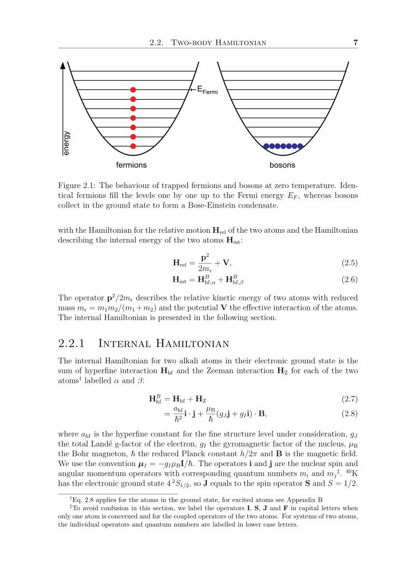
Figure 2.2: Hyperfine structure of 40K in the ground state |4 2S1/2〉. The states arelabelled a to r with rising energy and in the low-field basis |F,mF 〉. In the lowerhyperfine manifold, where F = 9/2, the states f to j are low-field seeking at lowmagnetic field. In the upper hyperfine manifold (F = 7/2) the states o to r are low-field seeking. The hyperfine structure is inverted unlike in most other alkalis. For moredetails see Appendix B.
The nuclear spin of 40K is I = 4. The energy eigenvalues of the internal Hamiltonianof a 40K atom are shown in Fig. 2.2. The states are labelled with the low-field basis|F,mF 〉 quantum numbers, where F = I + J and alphabetically with rising energy.
The hyperfine constant of 40K is ahf = h × −285.7308(24)MHz, resulting in ahyperfine splitting ∆Ehf = h× 1285.79MHz of the two hyperfine manifolds. Note thatthe hyperfine structure is inverted unlike in most other alkalis [Zac42]. In Appendix Bthe hyperfine structure of 40K is described in more detail and values for all relevantconstants are given.
The internal Hamiltonian in Eq. 2.6 can be separated into a term which conservesthe total electron spin H+
int and a term H−int which couples the different spins. Thisis done for indistinguishable particles with j = s = 1/2 in the symmetrized basis|SMSIMI〉 with I = iα + iβ, S = sα + sβ and equal ahf , gJ and gI .
H+int = ahf
2~2 I · S + µB
~(gJS + gII) ·B (2.9)
H−int = ahf
2~2 (iα − iβ) · (sα − sβ) (2.10)
2.2.2 Hamiltonian for the relative motionThe effective interaction V in the Hamiltonian of the relative motion in Eq. 2.5 canbe expressed as the (central) Coulomb interaction V C(r) of the two atoms with inter-nuclear distance r and total spin S = sα + sβ.
V C(r) =∑S
|S〉VS(r) 〈S| = PsVs + PtVt. (2.11)
Depending on the coupling of the individual spins, the interaction potential VS(r) hasfor s = 1/2 atoms a singlet (S=0) or a triplet (S=1) character with the respective
2.3. Elastic collisions 9
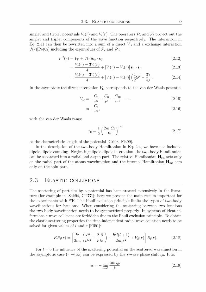
singlet and triplet potentials Vs(r) and Vt(r). The operators Ps and Pt project out thesinglet and triplet components of the wave function respectively. The interaction inEq. 2.11 can then be rewritten into a sum of a direct VD and a exchange interactionJ(r)[Pet02] including the eigenvalues of Ps and Pt:
V C(r) = VD + J(r)sα · sβ (2.12)
= Vs(r)− 3Vt(r)4 + [Vt(r)− Vs(r)] sα · sβ (2.13)
= Vs(r)− 3Vt(r)4 + [Vt(r)− Vs(r)]
(12S2 − 3
4
). (2.14)
In the asymptote the direct interaction VD corresponds to the van der Waals potential
VD = −C6
r6 −C8
r8 −C10
r10 − · · · (2.15)
≈ −C6
r6 , (2.16)
with the van der Waals range
r0 = 12
(2mrC6
~2
)1/4(2.17)
as the characteristic length of the potential [Gri93, Fla99].In the description of the two-body Hamiltonian in Eq. 2.4, we have not included
dipole-dipole coupling. Neglecting dipole-dipole interaction, the two-body Hamiltoniancan be separated into a radial and a spin part. The relative Hamiltonian Hrel acts onlyon the radial part of the atoms wavefunction and the internal Hamiltonian Hint actsonly on the spin part.
2.3 Elastic collisionsThe scattering of particles by a potential has been treated extensively in the litera-ture (for example in [Sak94, CT77]); here we present the main results important forthe experiments with 40K. The Pauli exclusion principle limits the types of two-bodywavefunctions for fermions. When considering the scattering between two fermionsthe two-body wavefunction needs to be symmetrized properly. In systems of identicalfermions s-wave collisions are forbidden due to the Pauli exclusion principle. To obtainthe elastic scattering properties the time-independent radial wave equation needs to besolved for given values of l and s [Fli91]:
ERl(r) =[
~2
2mr
(∂2
∂r2 + 2r
∂
∂r
)+ ~2l(l + 1)
2mrr2 + VS(r)]Rl(r). (2.18)
For l = 0 the influence of the scattering potential on the scattered wavefunction inthe asymptotic case (r →∞) can be expressed by the s-wave phase shift η0. It is:
a = − limk→0
tan η0
k(2.19)
10 2. Theoretical Background
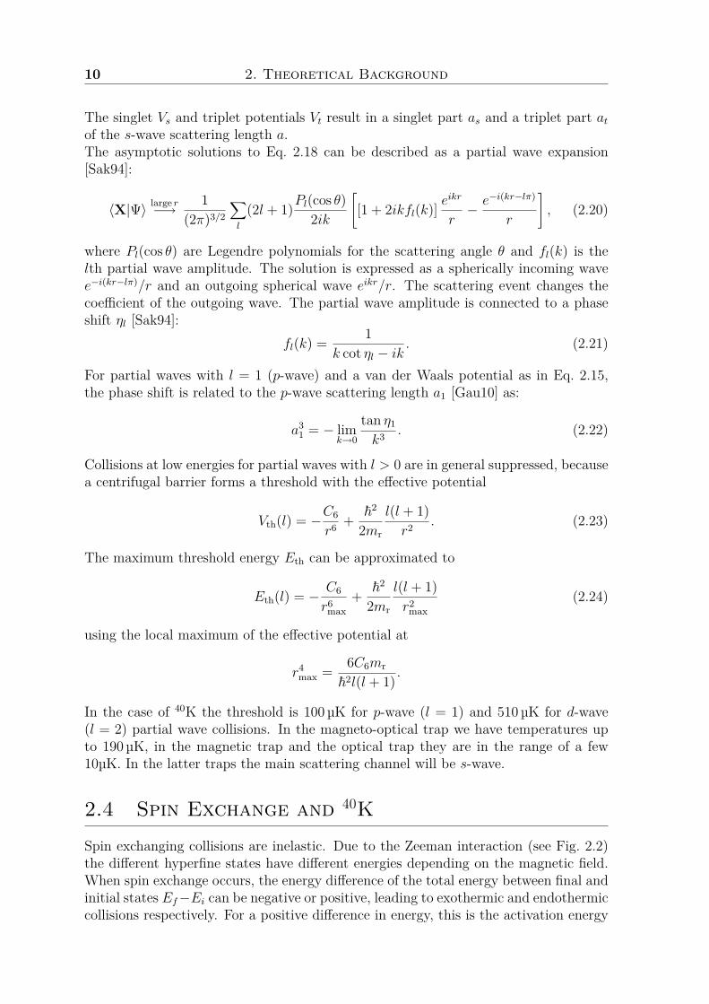
The singlet Vs and triplet potentials Vt result in a singlet part as and a triplet part atof the s-wave scattering length a.The asymptotic solutions to Eq. 2.18 can be described as a partial wave expansion[Sak94]:
〈X|Ψ〉 large r−→ 1(2π)3/2
∑l
(2l + 1)Pl(cos θ)2ik
[[1 + 2ikfl(k)] e
ikr
r− e−i(kr−lπ)
r
], (2.20)
where Pl(cos θ) are Legendre polynomials for the scattering angle θ and fl(k) is thelth partial wave amplitude. The solution is expressed as a spherically incoming wavee−i(kr−lπ)/r and an outgoing spherical wave eikr/r. The scattering event changes thecoefficient of the outgoing wave. The partial wave amplitude is connected to a phaseshift ηl [Sak94]:
fl(k) = 1k cot ηl − ik
. (2.21)
For partial waves with l = 1 (p-wave) and a van der Waals potential as in Eq. 2.15,the phase shift is related to the p-wave scattering length a1 [Gau10] as:
a31 = − lim
k→0
tan η1
k3 . (2.22)
Collisions at low energies for partial waves with l > 0 are in general suppressed, becausea centrifugal barrier forms a threshold with the effective potential
Vth(l) = −C6
r6 + ~2
2mr
l(l + 1)r2 . (2.23)
The maximum threshold energy Eth can be approximated to
Eth(l) = − C6
r6max
+ ~2
2mr
l(l + 1)r2
max(2.24)
using the local maximum of the effective potential at
r4max = 6C6mr
~2l(l + 1) .
In the case of 40K the threshold is 100µK for p-wave (l = 1) and 510µK for d-wave(l = 2) partial wave collisions. In the magneto-optical trap we have temperatures upto 190 µK, in the magnetic trap and the optical trap they are in the range of a few10µK. In the latter traps the main scattering channel will be s-wave.
2.4 Spin Exchange and 40KSpin exchanging collisions are inelastic. Due to the Zeeman interaction (see Fig. 2.2)the different hyperfine states have different energies depending on the magnetic field.When spin exchange occurs, the energy difference of the total energy between final andinitial states Ef−Ei can be negative or positive, leading to exothermic and endothermiccollisions respectively. For a positive difference in energy, this is the activation energy
2.4. Spin Exchange and 40K 11
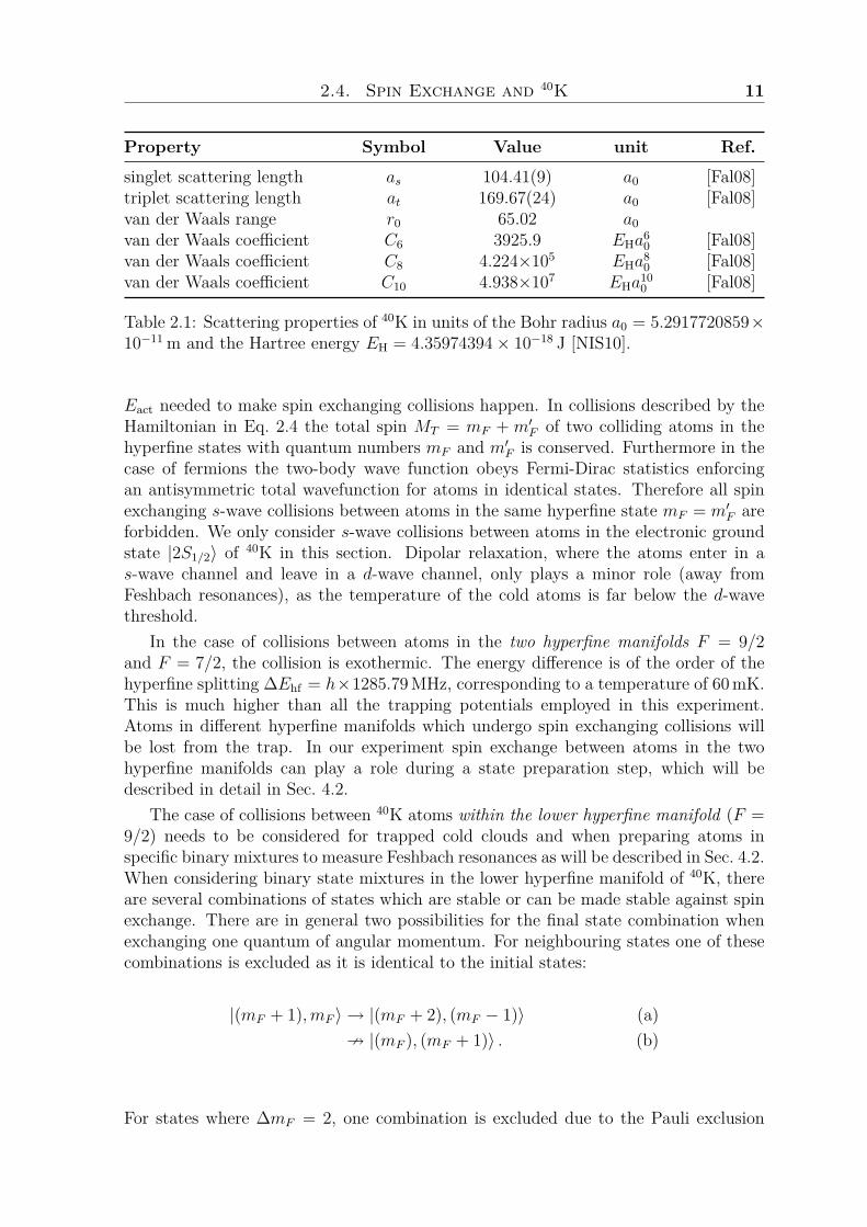
Property Symbol Value unit Ref.
singlet scattering length as 104.41(9) a0 [Fal08]triplet scattering length at 169.67(24) a0 [Fal08]van der Waals range r0 65.02 a0van der Waals coefficient C6 3925.9 EHa
60 [Fal08]
van der Waals coefficient C8 4.224×10⁵ EHa80 [Fal08]
van der Waals coefficient C10 4.938×10⁷ EHa100 [Fal08]
Table 2.1: Scattering properties of 40K in units of the Bohr radius a0 = 5.2917720859×10⁻¹¹ m and the Hartree energy EH = 4.35974394× 10⁻¹⁸ J [NIS10].
Eact needed to make spin exchanging collisions happen. In collisions described by theHamiltonian in Eq. 2.4 the total spin MT = mF + m′F of two colliding atoms in thehyperfine states with quantum numbers mF and m′F is conserved. Furthermore in thecase of fermions the two-body wave function obeys Fermi-Dirac statistics enforcingan antisymmetric total wavefunction for atoms in identical states. Therefore all spinexchanging s-wave collisions between atoms in the same hyperfine state mF = m′F areforbidden. We only consider s-wave collisions between atoms in the electronic groundstate |2S1/2〉 of 40K in this section. Dipolar relaxation, where the atoms enter in as-wave channel and leave in a d-wave channel, only plays a minor role (away fromFeshbach resonances), as the temperature of the cold atoms is far below the d-wavethreshold.
In the case of collisions between atoms in the two hyperfine manifolds F = 9/2and F = 7/2, the collision is exothermic. The energy difference is of the order of thehyperfine splitting ∆Ehf = h×1285.79MHz, corresponding to a temperature of 60mK.This is much higher than all the trapping potentials employed in this experiment.Atoms in different hyperfine manifolds which undergo spin exchanging collisions willbe lost from the trap. In our experiment spin exchange between atoms in the twohyperfine manifolds can play a role during a state preparation step, which will bedescribed in detail in Sec. 4.2.
The case of collisions between 40K atoms within the lower hyperfine manifold (F =9/2) needs to be considered for trapped cold clouds and when preparing atoms inspecific binary mixtures to measure Feshbach resonances as will be described in Sec. 4.2.When considering binary state mixtures in the lower hyperfine manifold of 40K, thereare several combinations of states which are stable or can be made stable against spinexchange. There are in general two possibilities for the final state combination whenexchanging one quantum of angular momentum. For neighbouring states one of thesecombinations is excluded as it is identical to the initial states:
|(mF + 1),mF 〉 → |(mF + 2), (mF − 1)〉 (a)9 |(mF ), (mF + 1)〉 . (b)
For states where ∆mF = 2, one combination is excluded due to the Pauli exclusion
12 2. Theoretical Background
i + f ® j + e
i + g ® j + fi + h ® j + g
h + f ® i + e
h + g ® i + f
0 200 400 600 800 10000
2000
4000
6000
8000
10 000
B @GD
Tac
t@Μ
KD
0 5 10 15 200
1
2
3
4
5
6
B @GD
Tac
t@Μ
KD
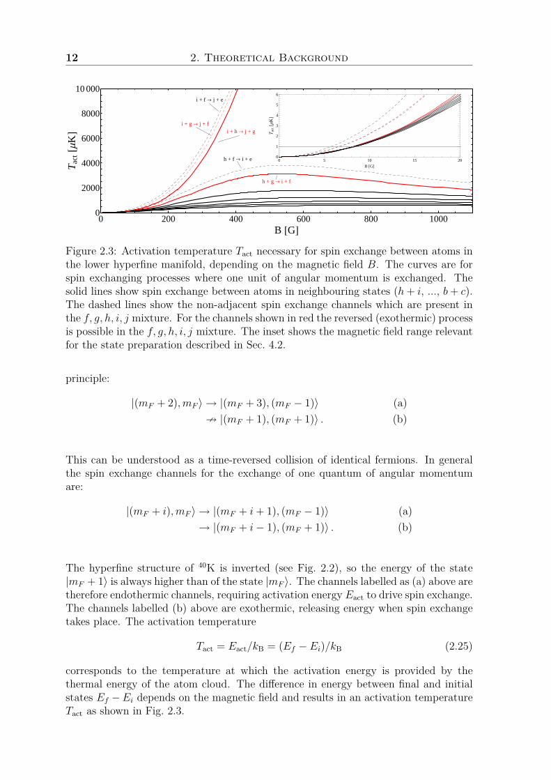
Figure 2.3: Activation temperature Tact necessary for spin exchange between atoms inthe lower hyperfine manifold, depending on the magnetic field B. The curves are forspin exchanging processes where one unit of angular momentum is exchanged. Thesolid lines show spin exchange between atoms in neighbouring states (h+ i, ..., b+ c).The dashed lines show the non-adjacent spin exchange channels which are present inthe f, g, h, i, j mixture. For the channels shown in red the reversed (exothermic) processis possible in the f, g, h, i, j mixture. The inset shows the magnetic field range relevantfor the state preparation described in Sec. 4.2.
principle:
|(mF + 2),mF 〉 → |(mF + 3), (mF − 1)〉 (a)9 |(mF + 1), (mF + 1)〉 . (b)
This can be understood as a time-reversed collision of identical fermions. In generalthe spin exchange channels for the exchange of one quantum of angular momentumare:
|(mF + i),mF 〉 → |(mF + i+ 1), (mF − 1)〉 (a)→ |(mF + i− 1), (mF + 1)〉 . (b)
The hyperfine structure of 40K is inverted (see Fig. 2.2), so the energy of the state|mF + 1〉 is always higher than of the state |mF 〉. The channels labelled as (a) above aretherefore endothermic channels, requiring activation energy Eact to drive spin exchange.The channels labelled (b) above are exothermic, releasing energy when spin exchangetakes place. The activation temperature
Tact = Eact/kB = (Ef − Ei)/kB (2.25)
corresponds to the temperature at which the activation energy is provided by thethermal energy of the atom cloud. The difference in energy between final and initialstates Ef −Ei depends on the magnetic field and results in an activation temperatureTact as shown in Fig. 2.3.
2.4. Spin Exchange and 40K 13
For binary mixtures consisting of neighbouring states or states with ∆mF = 2 itis always possible to stabilize the mixture by increasing the magnetic field or loweringthe temperature of the cold atom cloud. The activation temperature necessary Tact todrive spin exchange in mixtures of neighbouring states in the lower hyperfine manifoldis shown as solid lines in Fig. 2.3. The activation temperature Tact for states with∆mF = 2 is even higher. As mixtures of neighbouring states and of states with∆mF = 2 can be made stable, also mixtures of atoms in three adjacent states canbe stabilized. The fact that 40K is fermionic and has an inverted hyperfine structureallows for the realization of a multitude of stable state combinations, exceeding thepossibilities in other alkalis.
2.4.1 Populated states in the magnetic trapThe cold atoms in the magnetic trap (and in the optical dipole trap) are in the statesf, g, h, i, j (labelled as in Fig. 2.2). The combination |9/2 + 7/2〉 (j + i) is stableagainst spin exchanging collisions as there is no other combination with MT = 8.The binary mixture |9/2 + 5/2〉 (j + h) is stable against spin exchanging collisionsas the only possible final state combination is excluded due to the Pauli exclusionprinciple§. The mixture f, g, h, i, j has in total nine channels, where spin exchangings-wave collisions can exchange one unit of angular momentum between two atoms. Ofthose nine channels six are endothermic, the three remaining channels are exothermicand correspond to the reversed processes of endothermic channels.
Of the six endothermic channels, five involve neighbouring states or states with∆mF = 2. The dashed lines in Fig. 2.3 show the spin exchange channels present in thef, g, h, i, j mixture for non-adjacent states. The red lines correspond to the reverse ofthe three exothermic spin exchanging channels possible for atoms in the mixture. Theenergy release from the exothermic spin exchanging processes leads to loss from thetrap or – for low magnetic fields – a heating of the cold atom cloud.
2.4.2 Scattering rate for spin exchangeApart from the existence of decay channels, in an experiment the actual loss rate andwith that the stability of a mixture of two states is determined by the scattering rate.The two-body scattering rate K2, depends on the density of the involved states, thespatial overlap of the states and the difference between singlet and triplet scatteringlength [Pet02]:
K2 = 4π(as − at)2v′rel
∣∣∣〈F ′αm′F,α F ′βm′F,β|sα · sβ|FαmF,α FβmF,β〉∣∣∣2 , (2.26)
where |F ′αm′F,α F ′βm′F,β〉 and |FαmF,α FβmF,β〉 denote the final and initial hyperfinestates and v′rel is the relative velocity of the atoms in the final state. It is
v′rel =√
2mr
(Ekin + EHFα + EHF
β − EHF′α − EHF′
β ), (2.27)
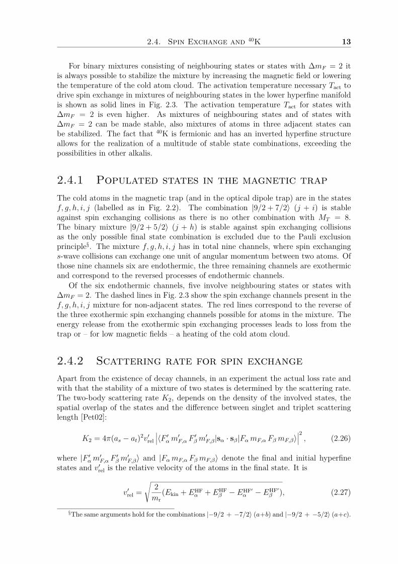
§The same arguments hold for the combinations |−9/2 + −7/2〉 (a+b) and |−9/2 + −5/2〉 (a+c).
14 2. Theoretical Background
with the reduced mass mr = (mαmβ)/(mα + mβ) and the kinetic energy Ekin of theinitial states. The energies EHF
i and EHF′i denote the hyperfine energies of the initial
and final states. To calculate the spin exchange rate between atoms of the sameatomic species, the hyperfine basis |FαmF,α FβmF,β〉 is transformed to the total spinbasis |SMS I MI〉.
From the factor (as − at)2 in Eq. 2.26 follows, that the two-body inelastic loss rateK2 is expected to be low, when the singlet and triplet scattering lengths are similar.This effect can also be understood as an interference effect as has been shown for 87Rb[Kok97, Bur97]. In the group at JILA [DeM01] an upper limit for the the non-resonantspin exchange rate in 40K was determined to be K2 < 2 × 10⁻¹⁴ cm3/s. Compared toother alkali atoms where K2 ≈ 10−11 cm3/s [Pet02], this is rather low.
2.5 Feshbach resonancesSo far we have covered the scattering properties for scattering from a central potential(Sec. 2.3). The potential determines the value of the scattering length a at low temper-atures. A form of resonant scattering are Feshbach resonances; they are an importanttool to control the interaction between ultracold atoms, as they allow to widely tunethe scattering length of the atoms.
In the asymptotic case (r → ∞) the hyperfine energy of the two colliding atomswith distance r determines the total energy of the atom pair. The total energy ofthe unbound pair forms the so-called open channel, as (s-wave) collisions are alwayspossible even when T → 0. Feshbach resonances occur when in addition to the openchannel there is also a two-body bound potential, a so-called closed channel, present.All scattering potentials which have a higher asymptotic energy than the open channelare referred to as closed channels (see Fig. 2.4). Due to resonant coupling to a boundstate with binding energy Eb within a closed channel the scattering length a can diverge.
The divergence of the scattering length occurs when the bound state in the closedchannel shifts into resonance with the energy of the open channel. Due to the differencein magnetic field dependence of the open and closed channel, the closed channel canbe moved relative to the energy of the open channel by applying an external magneticfield. The bound state in the closed channel is resonant at a certain magnetic field B0,when there is a coupling between the open and the closed channel. At the resonanceat magnetic field B0 the scattering length diverges as shown in Fig. 2.5.
The theory of Feshbach resonances [Fes58, Fes62] was originally developed for nu-clear physics, where the resonances do not depend on an external magnetic field buton the energy of the scatterers. The application of Feshbach resonances to alter thesign and the strength of the interaction in ultracold atoms by changing an externalfield was proposed by [Tie92, Tie93]. The first experimental observation of this effectin ultracold atoms were made in 23Na [Ino98] and in 85Rb [Cou98]. A detailed reviewof Feshbach resonances in ultracold atoms is given in [Chi10].
If only one closed channel is present the scattering length can be expressed as thesum of a resonant part ares and the background scattering length abg originating fromthe open channel:
a(B) = abg + ares(B).
2.5. Feshbach resonances 15
atomic separation
ener
gy
0
0
closed channelEB
open channel
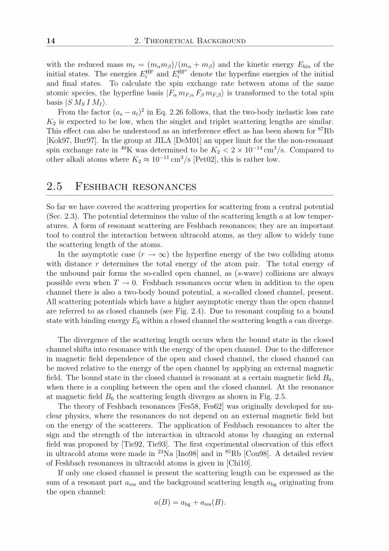
Figure 2.4: Two-channel model for a Feshbach resonance. When two atoms collide atenergy E in the open (entrance) channel (black curve), they can couple resonantly to abound state with binding energy Eb within a molecular potential (closed channel) (redcurve). The coupling leads to a diverging scattering length. If there is a difference inmagnetic moment of the open and the closed channel, the energy of the bound statein the closed channel can be tuned to cross the energy threshold of the two atoms bychanging the magnetic field.
The s-wave scattering in absence of inelastic two-body channels is described by [Moe95]
a(B) = abg
(1− ∆B
B −B0
), (2.28)
with the off-resonant background value of the scattering length abg, the Feshbach res-onance position B0 and its width ∆B. The width is defined via the position of thezero-crossing of the Feshbach resonance B(a = 0) = B0 + ∆B. The behaviour of thescattering length around a Feshbach resonance is shown in Fig. 2.5. The scatteringcross section is given by:
σ = g4πa2
1 + k2a2 = g4πa2
bg
(1− ∆B
B−B0
)2
1 + k2a2bg
(1− ∆B
B−B0
)2 , (2.29)
where k is the momentum and g is a symmetry factor. It is g = 1, except for thecase of two identical atoms (same species and same state) in a Maxwellian gas [Chi10].The difference in magnetic moment between the open and the closed channel ∆µ =µ0−µc = −∂Eb/∂B describes the coupling strength C between the open and the closedchannel.
C ≡ abg∆B∆µ.Further useful expressions to describe a Feshbach resonance are the length scale [Pet04]
R∗ ≡ ~2
2mrabg∆B∆µ,
the widthΓ ≡ ~2k
mrR∗= 2Ck
16 2. Theoretical Background
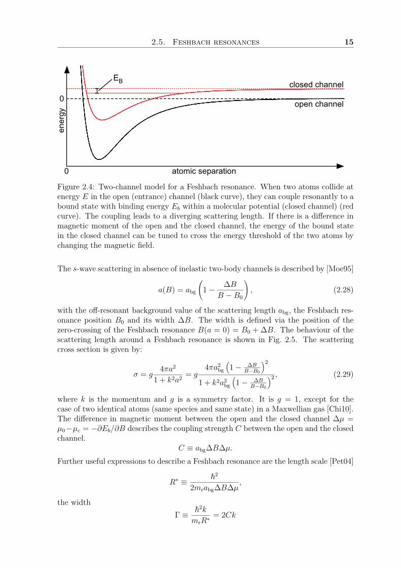
(B-B0)/DB
a/a bg
Figure 2.5: Divergence of the s-wave scattering length a around a Feshbach resonanceat the magnetic field B0.
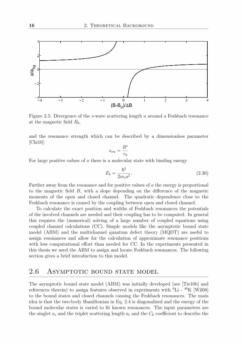
and the resonance strength which can be described by a dimensionless parameter[Chi10]:
sres = R∗
r0
For large positive values of a there is a molecular state with binding energy
Eb = ~2
2mra2 . (2.30)
Further away from the resonance and for positive values of a the energy is proportionalto the magnetic field B, with a slope depending on the difference of the magneticmoments of the open and closed channel. The quadratic dependence close to theFeshbach resonance is caused by the coupling between open and closed channel.
To calculate the exact position and widths of Feshbach resonances the potentialsof the involved channels are needed and their coupling has to be computed. In generalthis requires the (numerical) solving of a large number of coupled equations usingcoupled channel calculations (CC). Simple models like the asymptotic bound statemodel (ABM) and the multichannel quantum defect theory (MQDT) are useful toassign resonances and allow for the calculation of approximate resonance positionswith less computational effort than needed for CC. In the experiments presented inthis thesis we used the ABM to assign and locate Feshbach resonances. The followingsection gives a brief introduction to this model.
2.6 Asymptotic bound state modelThe asymptotic bound state model (ABM) was initially developed (see [Tie10b] andreferences therein) to assign features observed in experiments with 6Li - 40K [Wil08]to the bound states and closed channels causing the Feshbach resonances. The mainidea is that the two-body Hamiltonian in Eq. 2.4 is diagonalized and the energy of thebound molecular states is varied to fit known resonances. The input parameters arethe singlet as and the triplet scattering length at and the C6 coefficient to describe the
2.7. Trapped fermions 17
van der Waals tail of the interatomic potential. It is not necessary to solve the radialSchrödinger equation.
The model is called asymptotic because it is assumed that the detailed behaviourof the potential at small interatomic distances can be neglected as the main contribu-tion to the position of Feshbach resonances stems from the asymptotic behaviour ofthe atoms. In the course of diagonalizing the Hamiltonian, the overlap between thewavefunction in the singlet Vs and the triplet potential Vt needs to be computed. Thisoverlap is ≈ 1. For a first calculation of the position of Feshbach resonances thereare thus only three input parameters necessary. The calculation can be improved byoptimizing the overlap and the bound state energies of the molecular bound states tofit data determined in experiments. With the improved assumptions for the energiesand the overlap, the position of other Feshbach resonances can be determined. TheABM has the advantage that all possible resonances, however narrow, will be pre-dicted with relatively little computational effort. These results can then be used asinput for the exact coupled channel calculations. The assignment of s- and p-wave isalso immediately clear with ABM.
The ABM has been applied to mixtures of 6Li - 40K [Wil08, Tie10c], 85Rb - 87Rb,6Li - 87Rb [Li08], 6Li - 85Rb [Deh10], 40K - 87Rb [Tie10c], 3He∗ - 4He∗ [Goo10] and to23Na [Kno11]. The original ABM has been extended to also include dipole-dipole inter-actions and overlapping resonances [Goo10], and radio-frequency induced resonances[Tsc10]. The ABM is also used to calculate the widths of resonances [Tie10c]. Thisinvolves rewriting the Hamiltonian in terms of the closed and open channel contri-butions and extracting the coupling between them. For the individual mixtures andspecies some adaptations have to be made, it turns out that for 6Li - 40K one boundstate is sufficient. In 40K two bound states play a role as well as the large backgroundscattering length (see Sec. 5.3.3).
In our experiment we used the ABM together with values of the four resonancesknown at that time as well as the input parameters as, at and C6 from moleculespectroscopy [Fal08] to get initial predictions for Feshbach resonances in the hyperfinestate mixtures of 40K. Once new measurements were obtained, the overlap and bindingenergies were optimised (see Sec. 5.3.3) and further predictions for other hyperfine statemixtures were calculated.
2.7 Trapped fermions
We use magnetic and optical traps to confine the 40K. These trapping potentials aredescribed in detail in the appendices A and B. The potential has an effect on thedensity of states and with that on the Fermi energy EF. As depicted in Fig. 2.1, theFermi energy EF is defined as the energy of the highest state in a potential occupiedat T = 0. The Fermi temperature is defined accordingly as TF = EF/kB. For an idealgas in a trapping potential U(r), the density of states is
g(ε) = 1h3
∫δ
(ε−
[p2
2m + U(r)])
dpdr. (2.31)
18 2. Theoretical Background
From the definition of the Fermi energy follows the total number of atoms N :
N ≡∫ EF
0g(ε) dε. (2.32)
With Eq. 2.31 and 2.32 and a known potential the Fermi energy EF can be calcu-lated. The optical dipole trap used in our experiment, can be approximated at lowtemperatures by a harmonic potential¶, with
UODT(x, y, z) = m
2 (ω2rx
2 + ω2ry
2 + Aω2rz
2)
this results in the density of states [But97]
gODT(ε) = ε2
2A(~ωr)3 (2.33)
andEF = ~ωr(6AN)1/3, (2.34)
where A = ωz/ωr is the aspect ratio of the optical dipole trap, and the trapping fre-quencies are determined by the mass of the atoms and the laser detuning as described inAppendix A. For the linear magnetic trap as employed in the experiment (see Sec. 3.5.1and B.3) with a potential of the form
UMT(x, y, z) = U0
2√x2 + y2 + 4z2,
the density of states is given by [Bag87]:
gMT(ε) = 16√
2105π
(2√m
~U0
)3
ε7/2. (2.35)
The Fermi energy in this case is
EF ≈ 1.5962N2/9(
~U0√m
)2/3
. (2.36)
2.7.1 Fermi degenerate density distributionFor an ideal gas below the Fermi temperature TF the distribution is a Fermi-Diracdistribution
fFD(ε) = 11ζeε/kBT + 1 , (2.37)
with the fugacity ζ ≡ exp (µ/kBT ) depending on the chemical potential µ.To calculate the density distribution of a degenerate gas in a potential, a semi-
classical approximation can be used as long as the thermal energy of the gas kBT is¶The atoms in the optical dipole trap are in a Gaussian potential, which can be approximated
harmonically for low atom temperatures. The density distribution for thermal atoms in a Gaussianpotential is described in Appendix A.
2.7. Trapped fermions 19
much larger than the spacing ~ω of the (quantum mechanical) levels of the trappingpotential U(r). In this case the density distribution is given by:
nFD(r) = 1h3
∫ 1e(H(p,r)−µ)/kBT + 1 dp. (2.38)
Integration over all possible momenta p results in the density distribution of a degen-erate cloud of fermions at finite temperatures 0 < T < TF :
nFD(r) = −(
2πmkBT
h
)3/2
Li3/2(−ζe−U(r)/kBT ), (2.39)
with the polylogarithm function (Jonquière’s function) Lin(x) ≡ ∑∞k=1 x
k/kn. Thenumber of atoms for a harmonic confinement is obtained by integrating Eq. 2.39 overr:
N = − 1A
(kBT
~ωr
)3
Li3(−ζ). (2.40)
Combining this result with the Fermi energy kBTF in a harmonic trap Eq. 2.34 thefugacity depends only on T/TF:
T
TF= (−6 Li3(−ζ))−1/3 (2.41)
In the experiments we determine the density distribution by means of absorption imag-ing (see 3.8.3) along the axial direction of the dipole trap. This results in a projectionof the atom density on a two-dimensional optical density profile, which we can calculatefor a harmonic potential by integrating Eq. 2.34 over y‖.The imaging is usually done after releasing the atoms from the trap and some expan-sion of the cloud in time-of-flight. In the case of a harmonic trap it has been shown[Bru00], that the description of an ideal Fermi gas after free expansion only requires arescaling of the spatial coordinates xi in the density distribution Eq. 2.39, similar tothe bosonic case [Cas96, Kag96]. The rescaled coordinates x′i(t) are given by
x′i(t) = xi(0)√1 + ω2
i t2, (2.42)
when the harmonic trapping potential with trapping frequencies ωi is switched off att = 0. For a harmonic trap the cloud maintains the aspect ratio and shape it had inthe trap after free expansion. This shape invariance only holds for harmonic potentialsand simplifies the analysis of the absorption images tremendously. From the absorptionimages the number of atoms and the temperature of the cloud can be determined usingthe rescaled density profiles [But97, DeM01].
‖The axial (z-) direction of the dipole trap corresponds to the y-axis in the coordinate system ofthe experiment as depicted in Fig. 3.2.

Chapter 3
Experimental setup
3.1 Introduction
In this chapter the experimental setup is described. The experiments are done using theapparatus designed and developed for mixtures of ultracold 6Li and 40K. At the timethis apparatus was devised there were no other experiments on this specific mixture.Additionally, the scattering properties between the atomic species were not yet known,so the design had to make allowances for possible slow thermalization between thespecies. Recently the groups in Munich, in Innsbruck, at the MIT and in Paris havealso built experiments for 6Li and 40K. The group in Munich [Tag06] included 87Rb asa third atomic species in their setup to ensure efficient cooling. 87Rb had been broughtto degeneracy previously together with both 40K [Roa02, Ino04] and 6Li [Sil05], afterthe interspecies scattering lengths had been determined [Fer02, Sil05]. In the groupin Innsbruck an all-optical approach was chosen, resulting in large numbers of 6Liand low numbers of 40K. In that experiment efficient thermalization of the sampleis ensured by evaporating on the high-field side of a Feshbach resonance in lithiumat 834G [Wil08, Spi09]. The potassium is kept in the lowest hyperfine state and issympathetically cooled by the lithium. In the group at the MIT the bosonic isotope41K is used as a coolant [Wu11]. The group in Paris chose an approach similar to ours[Rid11b, Rid11a], relying on the thermalization between 6Li and 40K.
We decided on a setup which combines magnetic and optical trapping. A magnetictrap can be efficiently loaded from a magneto-optical trap (MOT) and provides largeatom numbers [Ono00, Sta07]. An optical dipole trap has the advantage that allhyperfine states can be trapped and the trapping potential is identical for all statesof one atomic species. Loading the dipole trap from a magnetic trap requires lessoptical power and a smaller trapping volume than loading it directly from a MOT.Two aspects of the design make the cold atoms easily (optically) accessible: firstly weuse an optically plugged magnetic trap [Dav95a] instead of a more commonly used Ioffe-Pritchard type trap [Pri83]. Secondly the optical dipole trap is employed as opticaltweezers to transport the atoms [Gus01] to a science cell where the experiments aredone. In many cold atom experiments magnetic transport is employed instead, in whicha cascade of coils or moving coils are used to transfer the atoms [Gre01]. The sciencecell is a quartz cell offering good optical access with a small working distance for the
22 3. Experimental setup
optics.Producing samples of ultracold atoms requires a vacuum system, lasers tuned close
to the transition frequencies of the atoms, a magnetic trap, an off-resonant opticaldipole trap or a combination of both to cool the gas close to degeneracy.
Much of the experimental setup has already been described in detail in the thesis ofT.G. Tiecke [Tie09a]. The present chapter summarizes the experimental setup puttingemphasis on added components and the parts essential for the experiments describedin this thesis. In section 3.2 the vacuum system is described, the laser system is coveredin section 3.3 and the magneto-optical trap in section 3.4. In section 3.5 the opticallyplugged magnetic trap is explained including its fast switching electronics. Our opticaldipole trap and the feedback circuit with large dynamic range used to stabilize itsintensity are presented in section 3.6. The coils used to produce homogeneous andstable magnetic fields for Feshbach measurements are covered in section 3.7. Theexperimental sequence, the preparation and detection of the Zeeman states and thecalibration of the Feshbach coils are described in Chapter 4.
3.2 Vacuum system
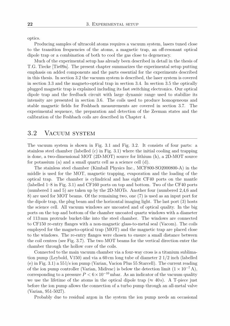
The vacuum system is shown in Fig. 3.1 and Fig. 3.2. It consists of four parts: astainless steel chamber (labelled (c) in Fig. 3.1) where the initial cooling and trappingis done, a two-dimensional MOT (2D-MOT) source for lithium (h), a 2D-MOT sourcefor potassium (a) and a small quartz cell as a science cell (d).
The stainless steel chamber (Kimball Physics Inc., MCF800-SO2000800-A) in themiddle is used for the MOT, magnetic trapping, evaporation and the loading of theoptical trap. The chamber is cylindrical and has eight CF40 ports on the mantle(labelled 1–8 in Fig. 3.1) and CF160 ports on top and bottom. Two of the CF40 ports(numbered 1 and 5) are taken up by the 2D-MOTs. Another four (numbered 2,4,6 and8) are used for MOT beams. Of the remaining two, one (7) is used as an input port forthe dipole trap, the plug beam and the horizontal imaging light. The last port (3) hoststhe science cell. All vacuum windows are uncoated and of optical quality. In the bigports on the top and bottom of the chamber uncoated quartz windows with a diameterof 113mm protrude bucket-like into the steel chamber. The windows are connectedto CF150 re-entry flanges with a non-magnetic glass-to-metal seal (Vacom). The coilsemployed for the magneto-optical trap (MOT) and the magnetic trap are placed closeto the windows. The re-entry flanges were chosen to ensure a small distance betweenthe coil centres (see Fig. 3.7). The two MOT beams for the vertical direction enter thechamber through the hollow core of the coils.
Connected to the main vacuum chamber via a four-way cross is a titanium sublima-tion pump (Leybold, V150) and via a 60 cm long tube of diameter 2 1/2 inch (labelled(e) in Fig. 3.1) a 55 l/s ion pump (Varian, Vacion Plus 55 Starcell). The current readingof the ion pump controller (Varian, Midivac) is below the detection limit (1× 10⁻⁷ A),corresponding to a pressure P < 6×10⁻¹⁰ mbar. As an indicator of the vacuum qualitywe use the lifetime of the atoms in the optical dipole trap (≈ 40 s). A T-piece justbefore the ion pump allows the connection of a turbo pump through an all-metal valve(Varian, 951-5027).
Probably due to residual argon in the system the ion pump needs an occasional

3.2. Vacuum system 23
Figure 3.1: The vacuum system as seen from above schematically: (a) potassium 2D-MOT source, (b) lithium 2D-MOT source, (c) main vacuum chamber, (d) science cell,(e) CF63 tube to the main 55 l/s ion pump, (f) CF40 tube leading to the 40 l/s ionpump (g) and (h) titanium sublimation pumps (mounted vertically), (i) direction ofview in Fig. 3.7 and (j) gate valve between lithium 2D-MOT and main chamber. Thisfigure is taken from [Tie09a].
bake-out. The argon saturates the ion pump and reduces the ultimate vacuum. In theexperiment it is then noticeable that the lifetime of the atoms in the optical dipoletrap shortens to ≈ 15 s. A bake-out of the ion pump was necessary every 6 – 9 months.Argon was introduced into the system during the first bake-out of the vacuum system[Tie09a] and has since then been pumped by the ion pump through the differentialpumping section connecting the 40K 2D-MOT to the main chamber. When a bake-outof the ion pump is necessary, it is heated to just below 400 C for several hours whilea turbo-molecular pump disposes of the gas load. As the ion pump is cooling down,the titanium sublimation pump connected to the main chamber is run for about oneminute at 50A, after degassing it at 25A.
The lithium 2D-MOT is pumped by a 40 l/s ion pump (Varian, Vacion Plus 40Starcell) and another titanium sublimation pump (Leybold, V150)(h). This titaniumpump was never used since the initial bake-out and the ion pump shows no load whenthe lithium oven is heated. This confirms the reputation of alkalis as efficient gettersin high-vacuum applications. The lithium 2D-MOT can be separated from the rest ofthe vacuum system with a gate valve (Leybold, UHV 28699).
Attached to the main chamber via a glass-to-metal transition is the quartz sciencecell with a length of 42mm and a 12.7mm2 cross-sectional area produced by TechglassInc. (in Aurora, Colorado, USA). The science cell allows for excellent optical access.Coils designed to produce a highly homogeneous magnetic field to measure Feshbachresonances are built around the science cell (see section 3.7).
The potassium 2D-MOT cell is custom-made of glass by Techglass. A four-waycross with optical quality windows (diameter 30mm) provides access for the four 2D-
24 3. Experimental setup
(g)
(b)
(c)
(d)
(a)
(e)
(f)
(h)(j)
(i)
x
y
z
Figure 3.2: Photograph of the vacuum system. The parts are labelled (a) to (j) as inFig. 3.1.
MOT beams cooling the atoms in radial direction (see Fig. 3.5 and Fig. 3.6). The cellis connected via a glass-to-metal transition to a CF40 flange. A differential pumpingsection of 23mm length and 2mm diameter connects the 2D-MOT to the the mainchamber. Mounted in front of the differential pumping tube is a gold mirror with a2mm hole in its centre. A distance of 2mm between the back of the mirror and thedifferential pumping tube ensures efficient pumping between the two surfaces. Thegold mirror can be used to reflect a probe beam or a one-dimensional optical molassesbeam. Opposing the mirror on the other end of the 2D-MOT cell is a fifth opticalquality window which is used for probe, cooling and push beams along the axis of the2D-MOT.
Connected to the side of the 2D-MOT cell is a glass tube of 13mm diameter leadingvia a T-piece to a break-seal ampule containing 40K-enriched potassium. The glasstube ends via a glass-to-metal transition and bellows in a CF16 flange. The flangewas initially intended to pump the 2D-MOT cell but was never used during the bakingand remains sealed with a valve [Tie09a]. As a source for the 40K we us KCl enrichedto an abundance of 6% 40K (Trace Science International). The distillation into thebreak-seal ampule was done by Techglass. To achieve the necessary vapour pressure inthe 2D-MOT, the entire cell is heated with heater tape and insulated with aluminiumfoil.
To complete the description of the vacuum system, it is mentioned that we havebuilt the first realisation of a 2D-MOT for lithium. It is fed by an effusive oven andresults in an output flux up to 3×10⁹/ s. Lithium reacts with glass, therefore we chosea stainless steel chamber for the lithium 2D-MOT. The windows admitting the MOTlight are under a 45 angle to the main axis of the lithium beam emitted from theoven, so the lithium cannot reach the windows under normal operation. The lithium
3.3. Laser system 25
clean
out
opt. p
umpin
g
imag
ing
push
repum
ptra
p
1 2 8 5 . 7 9 M H z
F = 9 / 2 ( - 5 7 1 . 4 6 2 M H z )
F ’ = 9 / 2 ( - 6 9 . 0 M H z )F ’ = 7 / 2 ( + 8 6 . 3 M H z )
F ’ = 9 / 2 ( - 2 . 3 M H z )F ’ = 7 / 2 ( 3 1 . 0 M H z )
F = 7 / 2 ( 7 1 4 . 3 2 8 M H z )
F ’ = 1 1 / 2 ( - 4 6 . 4 M H z )2 P 3 / 2
2 P 1 / 2
D 2 λ = 7 6 6 . 7 0 1 n m
D 1 λ = 7 7 0 . 1 0 8 n m
2 S 1 / 2
F ’ = 5 / 2 ( 5 5 . 2 M H z )
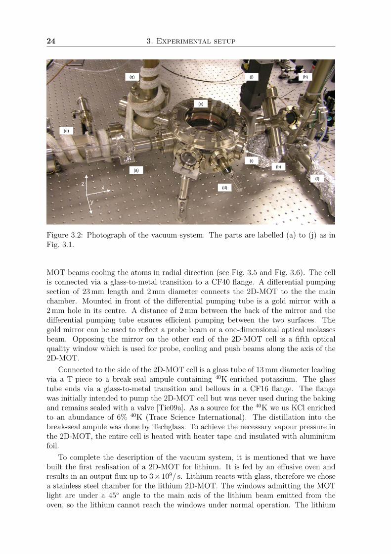
Figure 3.3: Optical spectrum of 40K with D1 and D2 lines. The transitions usedfor cooling, trapping and imaging are indicated. The numerical values originate from[Ari77] and [Fal06]. Unlike in other isotopes of potassium, the hyperfine structure isinverted in 40K.
2D-MOT is also connected to the main chamber via a differential pumping tube with agold mirror in front (identical to the potassium 2D-MOT). The principle is described indetail and predicted to work also for other light atomic species in [Tie09b] and [Tie09a].
3.3 Laser system
All manipulation of 40K with light is done on the D2 line, where we call the transi-tion |2S1/2, F = 9/2〉 → |2P3/2, F = 11/2〉 the trap transition and the |2S1/2, F = 7/2〉→ |2P3/2, F = 9/2〉 is referred to as the repump transition (see Fig. 3.3). Light withfrequencies tuned close to those transitions we refer to as trap and repump light respec-tively. In contrast to many other alkali isotopes, 40K has a sufficiently small hyperfinesplitting in the ground state (∆Ehf=1285.79MHz) to allow for the use of an acousto-optical modulator (AOM) to bridge the frequency difference.
One master laser (Toptica DLX110) is stabilized in frequency. The output power(350mW) is split into several beams, which are shifted by AOMs to the proper fre-quencies for the beams to trap, repump and image the atoms. To have sufficient power,the trap and repump light is amplified by tapered amplifiers. In Fig. 3.4 the simpli-

26 3. Experimental setup
fied optical setup is shown omitting beam-shaping optics and mirrors. The repumpfrequency is generated by shifting the master frequency by 1143MHz with an AOMfrom Brimrose (GPF-1240-200-766). All other frequencies used to manipulate the 40Kare obtained using AOMs by Isomet.
The DLX110 laser is stabilized to a polarization Zeeman spectroscopy. We lockthe laser to the unresolved |2S1/2, F = 1〉 → |2P3/2〉 transition in 39K. Light from themaster laser is brought via a polarization-maintaining fibre to a separate optical tableand its frequency is shifted by -260MHz with an AOM by Crystal Technologies. Thelinearly polarized light (≈ 200 µW) passes through a heated vapour cell (≈ 40 C)filled with potassium in natural abundance. A partial reflector (R = 10%) reduces thepower in the retro-reflected beam such that the two beams form a pump-probe setupof a Doppler-free saturation spectroscopy [Lev74, Bir74]. The vapour cell is placed in ahomogeneous magnetic field of a few Gauss. The field is parallel to the light, resulting inσ+ and σ− transitions (∆mF = ±1), being the allowed optical transitions. The σ+ andσ− transitions are shifted in frequency due to the Zeeman shift and differ in strengthdue to different Clebsch-Gordon coefficients. By placing a quarter waveplate and apolarizing cube in the path of the probe beam as shown in Fig. 3.4, the two circularpolarizations can be split and detected seperately by photodiodes (OPT101P-ND). Byelectronically subtracting the two photodiode signals a dispersive signal to lock the laseris retrieved. Two different stages stabilize the laser: one fast loop (bandwidth ≈ 4 kHz)feeds back to the diode current of the master laser and one slower loop (bandwidth≈ 1Hz) feeds back to the piezo-electric actuator controlling the grating position in theDLX110. The slow loop compensates for thermal drifts whereas the current feedbackensures short term stability.
The light for the trap and the repump beams is amplified by tapered amplifiers (Ea-gleyard, EYP-TPA-0765-01500-3006-CMT03-0000). The amplifier chips are mountedin a home-built aluminium housing, which we designed to ensure that thermal effectsdo not alter the position and consequently the injection of the amplifier. The mainfeature is that the chip is mounted such that any thermal expansion results in a minuterotation around the optical axis rather than a displacement. This rotation preservesthe injection of the laser beam in the amplifier chip and ensures constant power output.The temperature of the chip mount is stabilized with two thermo-electric Peltier ele-ments (Eureca Meßtechnik, TEC 1H-30-30-44/80-BS). The chip mount is electricallyinsulated from the aluminium housing by studs made from PEEK (polyether etherketone), a plastic with high tensile strength and small mechanical relaxation. Thecollimation lenses on both sides of the chip are also mounted on holders made fromPEEK. The threads on the lens holders are tightly fitted into the aluminium housing;for collimation the holder is simply wound in or out using a wrench. The design of themount and its thermal behaviour is described in some detail in [Koo07].
The tapered amplifier for the repump light is injected with 8mW and emits 200mW.The temperature is stabilized to 31 C by a temperature controller (Thorlabs, TED200C). The current through the chip (1.7A) is supplied by a home-built power sup-ply. The tapered amplifier for the trap light has both temperature and current (2A)stabilized by a laser controller (Sacher, Pilot 2000). It runs at 25 C, is injected with47mW and emits 767mW. Both tapered amplifiers only required re-adjustment of theinjection when the optical path before the amplifiers changed. The collimation hasstayed stable. The coupling efficiency into optical fibres is about 50%.

3.3. Laser system 27
high
-fiel
dim
agin
glo
w-fi
eld
imag
ing
∆ν
=2x
+56.
3MH
z
/4λ
4λ∆ν
=56
MH
z
Pol
pola
rizin
gcu
be
wav
epla
te
pola
rizer
optic
alis
olat
or
AO
M
phot
odio
de
fibre
coup
ler
lens
shut
ter
beam
split
ter
mirr
or
2λ
Topt
ica
DLX
110
∆ν
=-2
60M
Hz
Pol
4λK
vapo
urce
llR
=10%
spec
trosc
opy
on39
K
optic
alpu
mpi
ng
3D-M
OT
2D-M
OT
push
beam
∆ν
=+1
00M
Hz
2λ2λ
∆ν
=+9
4.1
MH
z
TA
∆ν
=-1
143M
Hz
TA
dark
repu
mpe
rbr
ight
repu
mpe
r
atom
rem
oval
∆ν
=+7
7.7
MH
z
∆ν
=+6
0.9
MH
z
/2λ
2λ
2λ
2λ
Figu
re3.4:
Optical
setupof
thelasers
ystem
for4
0 K.T
heTo
pticaDLX
110serves
asthemasterlaser.L
ight
fort
hetrap
andrepu
mp
tran
sitions
isam
plified
bytape
redam
plifiers(T
A).The
spectroscopy
setupislocatedon
asepa
rate
table.
Beam
shap
ingan
dfolding
optic
sha
vebe
enom
itted
from
this
schematic.
28 3. Experimental setup
3.4 Magneto-optical trapping
In a magneto-optical trap (MOT) neutral atoms are cooled by the absorption and re-emission of light and trapped in a steep magnetic gradient. The cooling mechanismworks due to radiation pressure from three orthogonal pairs of counter-propagatingbeams [Raa87, Met07]. Depending on the number of levels in the atomic spectrum andthe lifetimes and transition probabilities of the excited states, several optical transitionsneed to be driven by light. Successive absorption of light on a so-called cycle transition,enables the cooling. To achieve this in alkalis, two frequencies are needed: a trap (orcool) and a repump frequency. An atom moving towards the light beam is in resonancedue to the Doppler effect when the laser frequency is red detuned by several linewidthsΓ. Additionally the magnetic field gradient causes a spatially varying Zeeman shift ofthe transition frequencies and restricts the allowed optical transitions. If the counter-propagating beams have σ+ and σ− polarization, a moving atom will always be closerto being resonant with the light beam pushing the atom to the centre of the trap.Effectively the atoms are pushed to the centre of the trap where the magnetic fieldvanishes [Met99].
For the magneto-optical trapping of 40K the trap laser is red detuned by 6Γ fromthe |2S1/2, F = 9/2〉 −→ |2P3/2, F = 11/2〉 transition. The repump light is detuned by2Γ from the |2S1/2, F = 7/2〉 −→ |2P3/2, F = 9/2〉 transition. The detuning is chosento be identical for the two- and the three-dimensional MOT (3D-MOT).
3.4.1 Two-dimensional MOT for 40KAs sources for cold atoms, we employ a two-dimensional magneto-optical trap (2D-MOT). A great variety of sources for cold atoms have been developed over the years. Forpotassium custom-made dispensers are used alone [WI97, DeM99b], or in combinationwith light-induced atomic desorption (LIAD) [Goz93], as demonstrated in [Kle06] usingUV light. The resulting short vacuum lifetimes of using dispensers can be somewhatimproved [Moo05, Gri05] but the shortest loading times and highest atom numbersso far have been achieved with beam-loaded MOTs. The highest loading rates fordifferent atomic species have been achieved with a Zeeman slower [Lis99, Slo05, Sta05].However, the design of a Zeeman slower requires substantial engineering, especiallywhen recycling schemes or multiple species are used.
Compared to a Zeeman slower a 2D-MOT has the advantages that it is a compactsetup, it does not allow hot atoms into the main chamber and it makes most efficientuse of the atoms. Furthermore there are no stray magnetic fields close to the mainMOT. Especially in the case of potassium the high price of enriched potassium isan argument to use a 2D-MOT. The 2D-MOT is a two-dimensional realisation of aMOT. The circularly polarized light beams are applied from four (not six) directionsin space and the magnetic gradient is also two-dimensional as shown in Fig. 3.5. Thetwo-dimensional quadrupole field is zero along the symmetry axis. The MOT beamsdrive cold atoms towards this axis. Along the axial direction there is no confinementby magnetic fields. A push beam is used to push the atoms through the differentialpumping tube into the capture region of the 3D-MOT in the centre of the main chamber(see section 3.2). Some designs for 2D-MOTs employ an additional cooling beam

3.4. Magneto-optical trapping 29
differentialpumping section mirror
potassiumampule
with break seal
bellows
push beam
MOT beam
magnetencapsulated
in glass
valve
z
x
y
stack of permanentmagnets
MOT beam
2D quadrupolefield
(b) axial view(a) top view
z
yx
mirror
main vacuum chamber
Figure 3.5: Schematics of the 2D-MOT for 40K. The beams are retro-reflected and themagnetic field is formed by stacks of permanent magnets.
opposing the push beam creating a one-dimensional optical molasses [Die98, Cha06,Rid11b]; others are purely two-dimensional [Sch02]. For potassium 2D-MOTs are usedin Hamburg [Osp06b], Florence [Cat06] and Paris [Rid11b].
As described in section 3.2 we use two separate 2D-MOTs for the two species, theone for lithium is described in detail in [Tie09b]. Our source for the potassium is abreak-seal ampule, which was opened with a glass-encapsulated magnet also includedin the glass cell (see Fig. 3.6, Fig. 3.5 and Sec. 3.2). The glass cell of the 2D-MOT isheated to about 50 C to increase the vapour pressure. Two sets of permanent magnetsprovide the magnetic quadrupole field. The magnets are made of Nd2Fe14B (Eclipsemagnets, N750-RB) and their magnetisation has been measured to be 8.8(1)×105 A/m[Koo07]. Each set consists of two magnets separated by 12mm. A single magnet hasthe dimensions 25× 10× 3mm. Effectively the two magnets then form a 62mm longmagnetic dipole. The two magnet sets are each placed 35mm away from the axis ofthe cell and together form a radial gradient of 20G/cm. We use 120mW trap lightand 40mW repump light per beam. The beams are retro-reflected (see Fig. 3.5) andhave a 1/e-diameter of 18mm. For an improved loading of the 3D-MOT we employ apush beam, which is aligned along the axis of the 2D-MOT. The push beam consistsof 2.6mW of trap light detuned only by 2Γ from the trap transition. With this 2D-MOT we achieve loading rates in the 3D-MOT of 3 × 10⁸/s. This is over an orderof magnitude more than reported from Hamburg [OS06]. Recently the group in Paris[Rid11b] achieved 3D-MOT loading rates of 1.4× 10⁹/s using larger and more intense2D-MOT and 3D-MOT beams, and an additional molasses beam in the symmetry axis.
30 3. Experimental setup
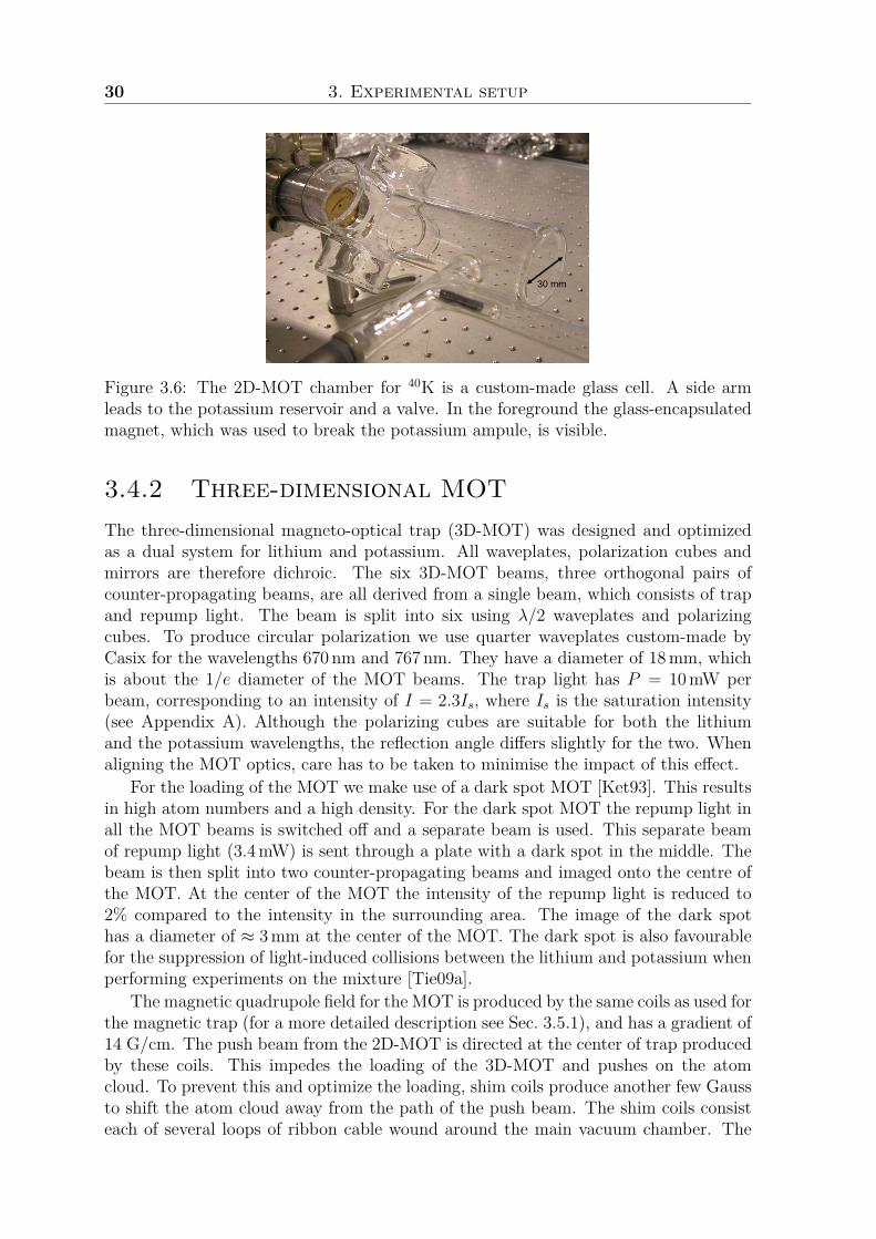
30 mm
Figure 3.6: The 2D-MOT chamber for 40K is a custom-made glass cell. A side armleads to the potassium reservoir and a valve. In the foreground the glass-encapsulatedmagnet, which was used to break the potassium ampule, is visible.
3.4.2 Three-dimensional MOTThe three-dimensional magneto-optical trap (3D-MOT) was designed and optimizedas a dual system for lithium and potassium. All waveplates, polarization cubes andmirrors are therefore dichroic. The six 3D-MOT beams, three orthogonal pairs ofcounter-propagating beams, are all derived from a single beam, which consists of trapand repump light. The beam is split into six using λ/2 waveplates and polarizingcubes. To produce circular polarization we use quarter waveplates custom-made byCasix for the wavelengths 670 nm and 767 nm. They have a diameter of 18mm, whichis about the 1/e diameter of the MOT beams. The trap light has P = 10mW perbeam, corresponding to an intensity of I = 2.3Is, where Is is the saturation intensity(see Appendix A). Although the polarizing cubes are suitable for both the lithiumand the potassium wavelengths, the reflection angle differs slightly for the two. Whenaligning the MOT optics, care has to be taken to minimise the impact of this effect.
For the loading of the MOT we make use of a dark spot MOT [Ket93]. This resultsin high atom numbers and a high density. For the dark spot MOT the repump light inall the MOT beams is switched off and a separate beam is used. This separate beamof repump light (3.4mW) is sent through a plate with a dark spot in the middle. Thebeam is then split into two counter-propagating beams and imaged onto the centre ofthe MOT. At the center of the MOT the intensity of the repump light is reduced to2% compared to the intensity in the surrounding area. The image of the dark spothas a diameter of ≈ 3mm at the center of the MOT. The dark spot is also favourablefor the suppression of light-induced collisions between the lithium and potassium whenperforming experiments on the mixture [Tie09a].
The magnetic quadrupole field for the MOT is produced by the same coils as used forthe magnetic trap (for a more detailed description see Sec. 3.5.1), and has a gradient of14 G/cm. The push beam from the 2D-MOT is directed at the center of trap producedby these coils. This impedes the loading of the 3D-MOT and pushes on the atomcloud. To prevent this and optimize the loading, shim coils produce another few Gaussto shift the atom cloud away from the path of the push beam. The shim coils consisteach of several loops of ribbon cable wound around the main vacuum chamber. The
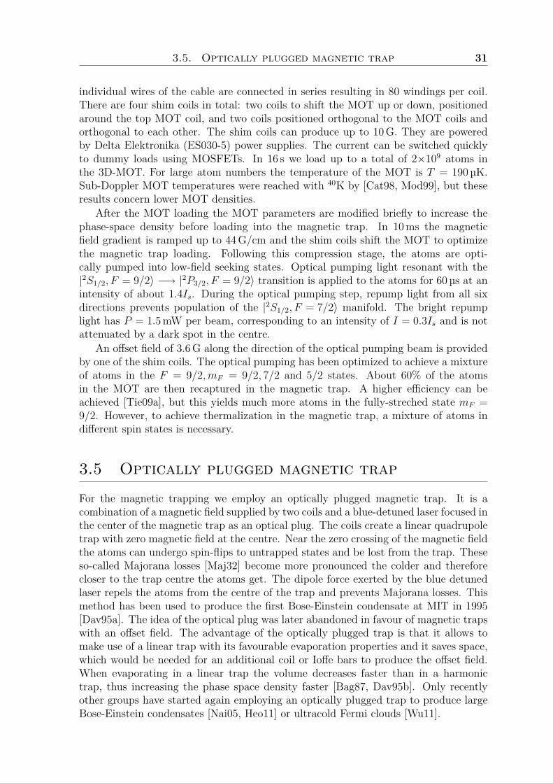
3.5. Optically plugged magnetic trap 31
individual wires of the cable are connected in series resulting in 80 windings per coil.There are four shim coils in total: two coils to shift the MOT up or down, positionedaround the top MOT coil, and two coils positioned orthogonal to the MOT coils andorthogonal to each other. The shim coils can produce up to 10G. They are poweredby Delta Elektronika (ES030-5) power supplies. The current can be switched quicklyto dummy loads using MOSFETs. In 16 s we load up to a total of 2×10⁹ atoms inthe 3D-MOT. For large atom numbers the temperature of the MOT is T = 190 µK.Sub-Doppler MOT temperatures were reached with 40K by [Cat98, Mod99], but theseresults concern lower MOT densities.
After the MOT loading the MOT parameters are modified briefly to increase thephase-space density before loading into the magnetic trap. In 10ms the magneticfield gradient is ramped up to 44G/cm and the shim coils shift the MOT to optimizethe magnetic trap loading. Following this compression stage, the atoms are opti-cally pumped into low-field seeking states. Optical pumping light resonant with the|2S1/2, F = 9/2〉 −→ |2P3/2, F = 9/2〉 transition is applied to the atoms for 60µs at anintensity of about 1.4Is. During the optical pumping step, repump light from all sixdirections prevents population of the |2S1/2, F = 7/2〉 manifold. The bright repumplight has P = 1.5mW per beam, corresponding to an intensity of I = 0.3Is and is notattenuated by a dark spot in the centre.
An offset field of 3.6G along the direction of the optical pumping beam is providedby one of the shim coils. The optical pumping has been optimized to achieve a mixtureof atoms in the F = 9/2,mF = 9/2, 7/2 and 5/2 states. About 60% of the atomsin the MOT are then recaptured in the magnetic trap. A higher efficiency can beachieved [Tie09a], but this yields much more atoms in the fully-streched state mF =9/2. However, to achieve thermalization in the magnetic trap, a mixture of atoms indifferent spin states is necessary.
3.5 Optically plugged magnetic trap
For the magnetic trapping we employ an optically plugged magnetic trap. It is acombination of a magnetic field supplied by two coils and a blue-detuned laser focused inthe center of the magnetic trap as an optical plug. The coils create a linear quadrupoletrap with zero magnetic field at the centre. Near the zero crossing of the magnetic fieldthe atoms can undergo spin-flips to untrapped states and be lost from the trap. Theseso-called Majorana losses [Maj32] become more pronounced the colder and thereforecloser to the trap centre the atoms get. The dipole force exerted by the blue detunedlaser repels the atoms from the centre of the trap and prevents Majorana losses. Thismethod has been used to produce the first Bose-Einstein condensate at MIT in 1995[Dav95a]. The idea of the optical plug was later abandoned in favour of magnetic trapswith an offset field. The advantage of the optically plugged trap is that it allows tomake use of a linear trap with its favourable evaporation properties and it saves space,which would be needed for an additional coil or Ioffe bars to produce the offset field.When evaporating in a linear trap the volume decreases faster than in a harmonictrap, thus increasing the phase space density faster [Bag87, Dav95b]. Only recentlyother groups have started again employing an optically plugged trap to produce largeBose-Einstein condensates [Nai05, Heo11] or ultracold Fermi clouds [Wu11].
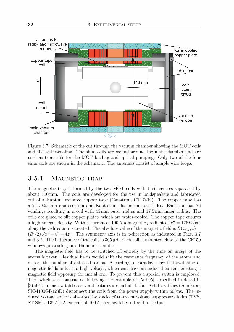
32 3. Experimental setup
main vacuumchamber
antennas forradio- and microwave
frequency
z
Figure 3.7: Schematic of the cut through the vacuum chamber showing the MOT coilsand the water-cooling. The shim coils are wound around the main chamber and areused as trim coils for the MOT loading and optical pumping. Only two of the fourshim coils are shown in the schematic. The antennas consist of simple wire loops.
3.5.1 Magnetic trapThe magnetic trap is formed by the two MOT coils with their centres separated byabout 110mm. The coils are developed for the use in loudspeakers and fabricatedout of a Kapton insulated copper tape (Canatron, CT 7419). The copper tape hasa 25×0.25mm cross-section and Kapton insulation on both sides. Each coil has 76windings resulting in a coil with 45mm outer radius and 17.5mm inner radius. Thecoils are glued to slit copper plates, which are water-cooled. The copper tape ensuresa high current density. With a current of 100A a magnetic gradient of B′ = 176G/cmalong the z-direction is created. The absolute value of the magnetic field is B(x, y, z) =(B′/2)
√x2 + y2 + 4z2. The symmetry axis is in z-direction as indicated in Figs. 3.7
and 3.2. The inductance of the coils is 365µH. Each coil is mounted close to the CF150windows protruding into the main chamber.
The magnetic field has to be switched off entirely by the time an image of theatoms is taken. Residual fields would shift the resonance frequency of the atoms anddistort the number of detected atoms. According to Faraday’s law fast switching ofmagnetic fields induces a high voltage, which can drive an induced current creating amagnetic field opposing the initial one. To prevent this a special switch is employed.The switch was constructed following the example of [Aub05], described in detail in[Stu04]. In one switch box several features are included: four IGBT switches (Semikron,SKM100GB123D) disconnect the coils from the power supply within 600 ns. The in-duced voltage spike is absorbed by stacks of transient voltage suppressor diodes (TVS,ST SM15T39A). A current of 100A then switches off within 100 µs.
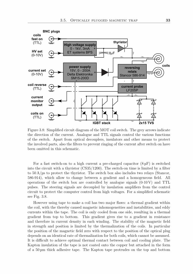
3.5. Optically plugged magnetic trap 33
coilsfast on(TTL) High voltage supply
0 - 1kV, 3mAET systems BPS
+
-HV set(0-10V)
coil reverse(TTL)
current set(0-10V)
coils on(TTL)
currentmonitoroutput
BNC plugs
reversingrelais
Stancor 586-914
current probeLF205P
power supply15V, 0 - 200A
Delta ElektronikaSM15-200D
+
-
2x15 TVSIGBT stack
coils
thyristor
8mF
Figure 3.8: Simplified circuit diagram of the MOT coil switch. The grey arrows indicatethe direction of the current. Analogue and TTL signals control the various functionsof the switch. Apart from optical decouplers, insulators and other means to protectthe involved parts, also the filters to prevent ringing of the current after switch on havebeen omitted in this schematic.
For a fast switch-on to a high current a pre-charged capacitor (8 µF) is switchedinto the circuit with a thyristor (CS35/1200). The switch-on time is limited by a filterto 50A/µs to protect the thyristor. The switch box also includes two relays (Stancor,586-914), which allow to change between a gradient and a homogeneous field. Alloperations of the switch box are controlled by analogue signals (0-10V) and TTLpulses. The steering signals are decoupled by insulation amplifiers from the controlcircuit to protect the computer control from high voltages. For a simplified schematicsee Fig. 3.8.
However using tape to make a coil has two major flaws: a thermal gradient withinthe coil, with the thereby caused magnetic inhomogeneities and instabilities, and eddycurrents within the tape. The coil is only cooled from one side, resulting in a thermalgradient from top to bottom. This gradient gives rise to a gradient in resistanceand therefore in current density in each winding. The stability of the magnetic fieldin strength and position is limited by the thermalization of the coils. In particularthe position of the magnetic field zero with respect to the position of the optical plugdepends on an identical rate of thermalization for both coils, which cannot be assumed.It is difficult to achieve optimal thermal contact between coil and cooling plate. TheKapton insulation of the tape is not coated onto the copper but attached in the formof a 50µm thick adhesive tape. The Kapton tape protrudes on the top and bottom

34 3. Experimental setup
of the coil. We have improved this by milling off the Kapton and placing 0.2mmthick electric insulation pads between cooling plate and the coils. The thick pads werenecessary because the contact surface is not entirely flat. However, the insulation limitsthe thermal conductance between the coils and cooling plates.
The heating of the MOT coils results in a decreased atom number if the coils runfor longer than usual (for example when measuring the lifetime in the magnetic trap).For a normal experimental cycle where the atoms are transferred from the magnetictrap to the dipole trap after 23 s and a new measurement starts about every minute,the temperature varies about 8 C. When running 100A through the coils, they heat upby about 35 C within 2 minutes. In addition the tape coils have the disadvantage thatthe switching-off induces eddy currents within the copper tape of the coils, which canpersist for a couple of milliseconds. The current only produces a small field, orthogonalto the dipole created by the coil itself. In practice a shift of the resonance frequency forthe imaging is not noticeable any longer after 2ms time-of-flight. We do not recommendthe use of copper tape with a large aspect ratio for coils in a magnetic trap.
3.5.2 Optical plug
The coils create a linear quadrupole trap with zero magnetic field at the centre. Toprevent Majorana losses at the zero-crossing we focus 9W of 532 nm laser light as anoptical plug in the centre of the trap. It is essential that the beam profile of the pluglaser is a Gaussian transverse electro-magnetic mode (TEM00). Dust on the opticsor thermal lensing in an AOM can lead to a doughnut shaped mode (TEM01), whichmakes the optical plug less efficient. To avoid this problem we have replaced the AOM,which was initially used to switch off the plug, by a high power shutter (nmLaserProducts Inc., LST4WBK2-D123). The shutter does not close sufficiently fast to beable to image the cloud in the main chamber after release from the magnetic trap.For alignment purposes it is best to leave the plug switched-on during time of flight.The imaging of the atoms then allows for qualitative measurements. All quantitativemeasurements are done releasing the atoms from the optical dipole trap with the opticalplug switched off.
As illustrated in Fig. 3.9 the beam mode and focus shape is monitored with a CCDcamera placed in the focus of the reflection from the beamsplitter which combines theoptical plug and the optical dipole trap just in front of the vacuum chamber. Thepassage through the beamsplitter introduces astigmatism to the plug beam profile,displacing the two foci by about 2.2mm. The average waist of the beam is w =16µm.The light for this optical plug is provided by a 10W Verdi (Coherent).
When running a high current through the MOT coils for times longer than 30 s,for instance when measuring the vacuum lifetime in the main chamber, the coils heatup noticeably and this affects the number of trapped atoms. This can be attributedto the thermalization of the coils. When heating up, the position of the magnetic fieldzero changes such that the alignment of the optical plug is not optimal any more andMajorana losses are not sufficiently suppressed. The alignment of the plug beam itselfis stable, we only have to adjust it every 4–6 weeks during normal operation.
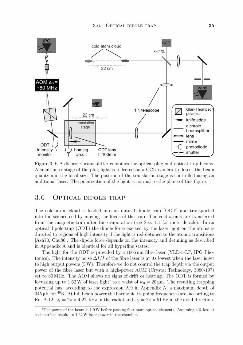
3.6. Optical dipole trap 35
photodiode
lens
shutter
dichroicbeamsplitter
mirror
knife edge
Glan-Thompsonpolarizer
homingcircuit
ODTintensitymonitor
IPG
VerdiAOM ∆ν=+80 MHz
translationstage
22 cm
22 cm
CCDcold atom cloud
<<1%
ODT lensf=100mm
1:1 telescope
Figure 3.9: A dichroic beamsplitter combines the optical plug and optical trap beams.A small percentage of the plug light is reflected on a CCD camera to detect the beamquality and the focal size. The position of the translation stage is controlled using anadditional laser. The polarization of the light is normal to the plane of this figure.
3.6 Optical dipole trap
The cold atom cloud is loaded into an optical dipole trap (ODT) and transportedinto the science cell by moving the focus of the trap. The cold atoms are transferredfrom the magnetic trap after the evaporation (see Sec. 4.1 for more details). In anoptical dipole trap (ODT) the dipole force exerted by the laser light on the atoms isdirected to regions of high intensity if the light is red-detuned to the atomic transitions[Ash70, Chu86]. The dipole force depends on the intensity and detuning as describedin Appendix A and is identical for all hyperfine states.
The light for the ODT is provided by a 1065 nm fibre laser (YLD-5-LP, IPG Pho-tonics). The intensity noise ∆I/I of the fibre laser is at its lowest when the laser is setto high output powers (5W). Therefore we do not control the trap depth via the outputpower of the fibre laser but with a high-power AOM (Crystal Technology, 3080-197)set to 80MHz. The AOM shows no signs of drift or heating. The ODT is formed byfocussing up to 1.62W of laser light† to a waist of w0 = 20 µm. The resulting trappingpotential has, according to the expression A.9 in Appendix A, a maximum depth of345µK for 40K. At full beam power the harmonic trapping frequencies are, according toEq. A.12, ωr = 2π× 4.27 kHz in the radial and ωa = 2π× 51Hz in the axial direction.
†The power of the beam is 1.9W before passing four more optical elements. Assuming 4% loss ateach surface results in 1.62W laser power in the chamber.
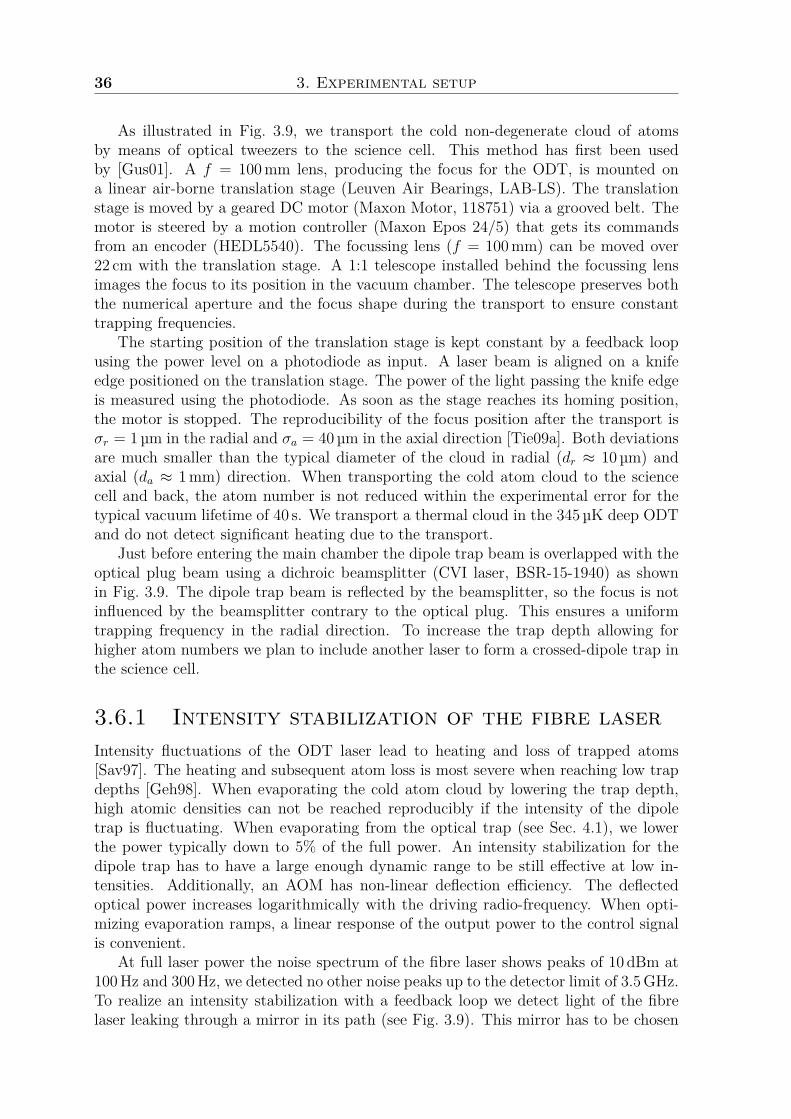
36 3. Experimental setup
As illustrated in Fig. 3.9, we transport the cold non-degenerate cloud of atomsby means of optical tweezers to the science cell. This method has first been usedby [Gus01]. A f = 100mm lens, producing the focus for the ODT, is mounted ona linear air-borne translation stage (Leuven Air Bearings, LAB-LS). The translationstage is moved by a geared DC motor (Maxon Motor, 118751) via a grooved belt. Themotor is steered by a motion controller (Maxon Epos 24/5) that gets its commandsfrom an encoder (HEDL5540). The focussing lens (f = 100mm) can be moved over22 cm with the translation stage. A 1:1 telescope installed behind the focussing lensimages the focus to its position in the vacuum chamber. The telescope preserves boththe numerical aperture and the focus shape during the transport to ensure constanttrapping frequencies.
The starting position of the translation stage is kept constant by a feedback loopusing the power level on a photodiode as input. A laser beam is aligned on a knifeedge positioned on the translation stage. The power of the light passing the knife edgeis measured using the photodiode. As soon as the stage reaches its homing position,the motor is stopped. The reproducibility of the focus position after the transport isσr = 1 µm in the radial and σa = 40 µm in the axial direction [Tie09a]. Both deviationsare much smaller than the typical diameter of the cloud in radial (dr ≈ 10 µm) andaxial (da ≈ 1mm) direction. When transporting the cold atom cloud to the sciencecell and back, the atom number is not reduced within the experimental error for thetypical vacuum lifetime of 40 s. We transport a thermal cloud in the 345µK deep ODTand do not detect significant heating due to the transport.
Just before entering the main chamber the dipole trap beam is overlapped with theoptical plug beam using a dichroic beamsplitter (CVI laser, BSR-15-1940) as shownin Fig. 3.9. The dipole trap beam is reflected by the beamsplitter, so the focus is notinfluenced by the beamsplitter contrary to the optical plug. This ensures a uniformtrapping frequency in the radial direction. To increase the trap depth allowing forhigher atom numbers we plan to include another laser to form a crossed-dipole trap inthe science cell.
3.6.1 Intensity stabilization of the fibre laserIntensity fluctuations of the ODT laser lead to heating and loss of trapped atoms[Sav97]. The heating and subsequent atom loss is most severe when reaching low trapdepths [Geh98]. When evaporating the cold atom cloud by lowering the trap depth,high atomic densities can not be reached reproducibly if the intensity of the dipoletrap is fluctuating. When evaporating from the optical trap (see Sec. 4.1), we lowerthe power typically down to 5% of the full power. An intensity stabilization for thedipole trap has to have a large enough dynamic range to be still effective at low in-tensities. Additionally, an AOM has non-linear deflection efficiency. The deflectedoptical power increases logarithmically with the driving radio-frequency. When opti-mizing evaporation ramps, a linear response of the output power to the control signalis convenient.
At full laser power the noise spectrum of the fibre laser shows peaks of 10 dBm at100Hz and 300Hz, we detected no other noise peaks up to the detector limit of 3.5GHz.To realize an intensity stabilization with a feedback loop we detect light of the fibrelaser leaking through a mirror in its path (see Fig. 3.9). This mirror has to be chosen
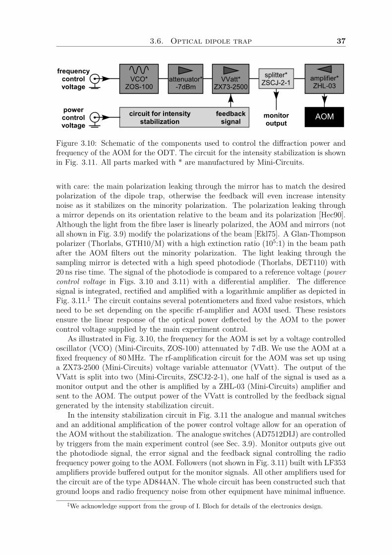
3.6. Optical dipole trap 37
AOM
amplifier*ZHL-03
splitter*ZSCJ-2-1VVatt*
ZX73-2500attenuator*
-7dBm
frequencycontrolvoltage
circuit for intensitystabilization
feedbacksignal
powercontrolvoltage
VCO*ZOS-100
monitoroutput
Figure 3.10: Schematic of the components used to control the diffraction power andfrequency of the AOM for the ODT. The circuit for the intensity stabilization is shownin Fig. 3.11. All parts marked with * are manufactured by Mini-Circuits.
with care: the main polarization leaking through the mirror has to match the desiredpolarization of the dipole trap, otherwise the feedback will even increase intensitynoise as it stabilizes on the minority polarization. The polarization leaking througha mirror depends on its orientation relative to the beam and its polarization [Hec90].Although the light from the fibre laser is linearly polarized, the AOM and mirrors (notall shown in Fig. 3.9) modify the polarizations of the beam [Ekl75]. A Glan-Thompsonpolarizer (Thorlabs, GTH10/M) with a high extinction ratio (105:1) in the beam pathafter the AOM filters out the minority polarization. The light leaking through thesampling mirror is detected with a high speed photodiode (Thorlabs, DET110) with20 ns rise time. The signal of the photodiode is compared to a reference voltage (powercontrol voltage in Figs. 3.10 and 3.11) with a differential amplifier. The differencesignal is integrated, rectified and amplified with a logarithmic amplifier as depicted inFig. 3.11.‡ The circuit contains several potentiometers and fixed value resistors, whichneed to be set depending on the specific rf-amplifier and AOM used. These resistorsensure the linear response of the optical power deflected by the AOM to the powercontrol voltage supplied by the main experiment control.
As illustrated in Fig. 3.10, the frequency for the AOM is set by a voltage controlledoscillator (VCO) (Mini-Circuits, ZOS-100) attenuated by 7 dB. We use the AOM at afixed frequency of 80MHz. The rf-amplification circuit for the AOM was set up usinga ZX73-2500 (Mini-Circuits) voltage variable attenuator (VVatt). The output of theVVatt is split into two (Mini-Circuits, ZSCJ2-2-1), one half of the signal is used as amonitor output and the other is amplified by a ZHL-03 (Mini-Circuits) amplifier andsent to the AOM. The output power of the VVatt is controlled by the feedback signalgenerated by the intensity stabilization circuit.
In the intensity stabilization circuit in Fig. 3.11 the analogue and manual switchesand an additional amplification of the power control voltage allow for an operation ofthe AOM without the stabilization. The analogue switches (AD7512DIJ) are controlledby triggers from the main experiment control (see Sec. 3.9). Monitor outputs give outthe photodiode signal, the error signal and the feedback signal controlling the radiofrequency power going to the AOM. Followers (not shown in Fig. 3.11) built with LF353amplifiers provide buffered output for the monitor signals. All other amplifiers used forthe circuit are of the type AD844AN. The whole circuit has been constructed such thatground loops and radio frequency noise from other equipment have minimal influence.
‡We acknowledge support from the group of I. Bloch for details of the electronics design.
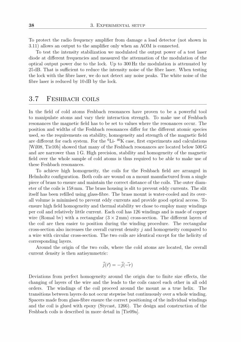
38 3. Experimental setup
To protect the radio frequency amplifier from damage a load detector (not shown in3.11) allows an output to the amplifier only when an AOM is connected.
To test the intensity stabilization we modulated the output power of a test laserdiode at different frequencies and measured the attenuation of the modulation of theoptical output power due to the lock. Up to 300Hz the modulation is attenuated by25 dB. That is sufficient to reduce the intensity noise of the fibre laser. When testingthe lock with the fibre laser, we do not detect any noise peaks. The white noise of thefibre laser is reduced by 10 dB by the lock.
3.7 Feshbach coils
In the field of cold atoms Feshbach resonances have proven to be a powerful toolto manipulate atoms and vary their interaction strength. To make use of Feshbachresonances the magnetic field has to be set to values where the resonances occur. Theposition and widths of the Feshbach resonances differ for the different atomic speciesused, so the requirements on stability, homogeneity and strength of the magnetic fieldare different for each system. For the 6Li- 40K case, first experiments and calculations[Wil08, Tie10b] showed that many of the Feshbach resonances are located below 500Gand are narrower than 1G. High precision, stability and homogeneity of the magneticfield over the whole sample of cold atoms is thus required to be able to make use ofthese Feshbach resonances.
To achieve high homogeneity, the coils for the Feshbach field are arranged inHelmholtz configuration. Both coils are wound on a mount manufactured from a singlepiece of brass to ensure and maintain the correct distance of the coils. The outer diam-eter of the coils is 158mm. The brass housing is slit to prevent eddy currents. The slititself has been refilled using glass-fibre. The brass mount is water-cooled and its over-all volume is minimised to prevent eddy currents and provide good optical access. Toensure high field homogeneity and thermal stability we chose to employ many windingsper coil and relatively little current. Each coil has 126 windings and is made of copperwire (Romal bv) with a rectangular (3 × 2mm) cross-section. The different layers ofthe coil are then easier to position during the winding procedure. The rectangularcross-section also increases the overall current density j and homogeneity compared toa wire with circular cross-section. The two coils are identical except for the helicity ofcorresponding layers.
Around the origin of the two coils, where the cold atoms are located, the overallcurrent density is then antisymmetric:
~j(~r) = −~j( ~−r)
Deviations from perfect homogeneity around the origin due to finite size effects, thechanging of layers of the wire and the leads to the coils cancel each other in all oddorders. The windings of the coil proceed around the mount as a true helix. Thetransitions between layers do not occur stepwise but continuously over a whole winding.Spacers made from glass-fibre ensure the correct positioning of the individual windingsand the coil is glued with epoxy (Stycast, 1266). The design and construction of theFeshbach coils is described in more detail in [Tie09a].
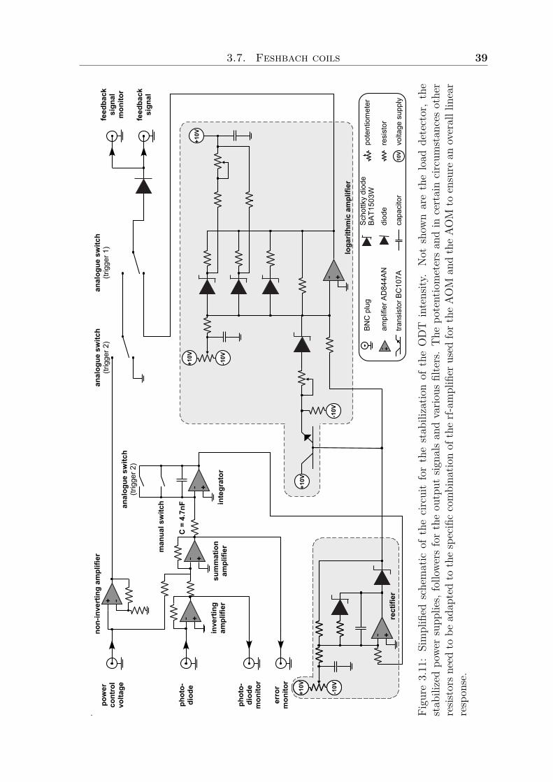
3.7. Feshbach coils 39
BN
Cpl
ug
+-am
plifi
erA
D84
4AN
trans
isto
rBC
107A
Sch
ottk
ydi
ode
BA
T150
3W
diod
e
capa
cito
r
pote
ntio
met
er
resi
stor
10V
volta
gesu
pply
-10V
+10V
+-re
ctifi
er
-10V
+10V
+-
-10V
+10V
-10V
+10V
+10V
+-
feed
back
sign
al
pow
erco
ntro
lvo
ltage
phot
o-di
ode
erro
rm
onito
r
phot
o-di
ode
mon
itor
feed
back
sign
alm
onito
r+ -
anal
ogue
switc
h(tr
igge
r2)
anal
ogue
switc
h(tr
igge
r1)
+-+-
+-
anal
ogue
switc
h(tr
igge
r2)
man
uals
witc
h
C=
4.7n
F
non-
inve
rtin
gam
plifi
er
inve
rtin
gam
plifi
ersu
mm
atio
nam
plifi
erin
tegr
ator
loga
rithm
icam
plifi
er
Figu
re3.11:Simplified
schematic
ofthecircuitforthestab
ilizatio
nof
theODT
intensity
.Not
show
naretheload
detector,the
stab
ilizedpo
wersupp
lies,
follo
wers
fortheou
tput
signa
lsan
dvario
usfilters.The
potentiometersan
din
certaincircum
stan
cesother
resis
tors
need
tobe
adap
tedto
thespecificcombina
tionof
therf-
amplifier
used
fort
heAOM
andtheAOM
toensure
anoveralllinear
respon
se.
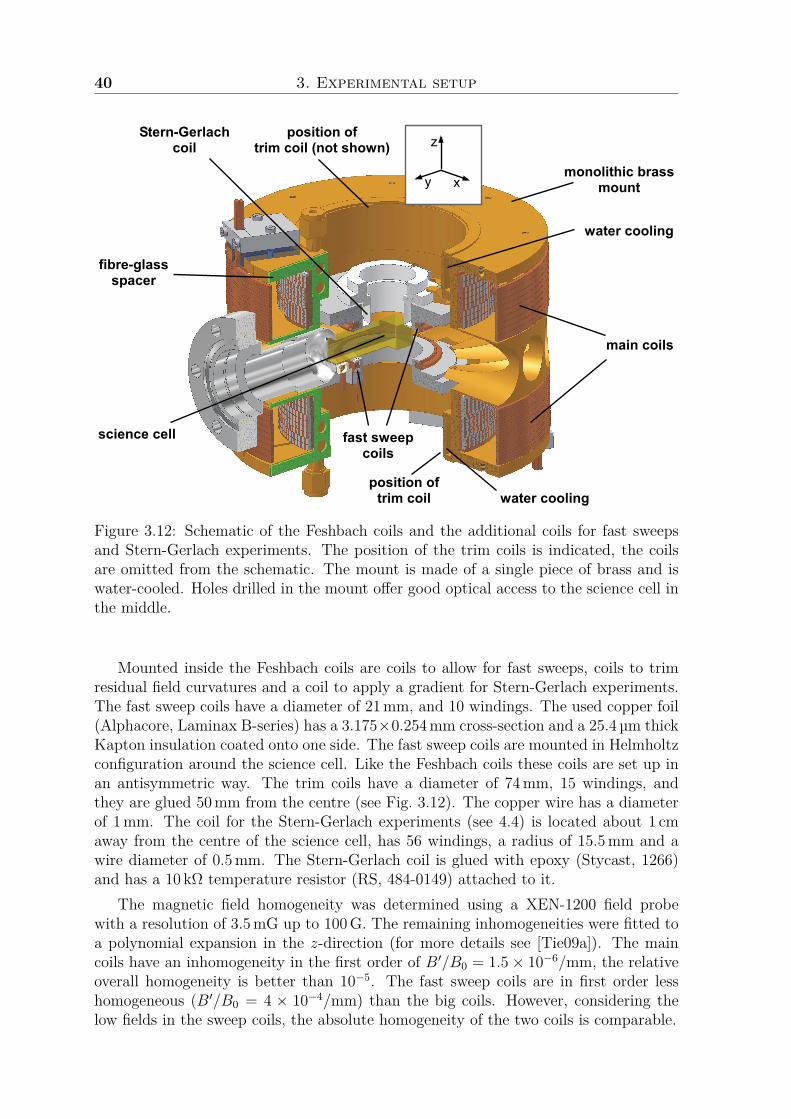
40 3. Experimental setup
main coils
fast sweepcoils
science cell
z
xy
Stern-Gerlachcoil
water cooling
water cooling
position oftrim coil (not shown)
position oftrim coil
fibre-glassspacer
monolithic brassmount
Figure 3.12: Schematic of the Feshbach coils and the additional coils for fast sweepsand Stern-Gerlach experiments. The position of the trim coils is indicated, the coilsare omitted from the schematic. The mount is made of a single piece of brass and iswater-cooled. Holes drilled in the mount offer good optical access to the science cell inthe middle.
Mounted inside the Feshbach coils are coils to allow for fast sweeps, coils to trimresidual field curvatures and a coil to apply a gradient for Stern-Gerlach experiments.The fast sweep coils have a diameter of 21mm, and 10 windings. The used copper foil(Alphacore, Laminax B-series) has a 3.175×0.254mm cross-section and a 25.4µm thickKapton insulation coated onto one side. The fast sweep coils are mounted in Helmholtzconfiguration around the science cell. Like the Feshbach coils these coils are set up inan antisymmetric way. The trim coils have a diameter of 74mm, 15 windings, andthey are glued 50mm from the centre (see Fig. 3.12). The copper wire has a diameterof 1mm. The coil for the Stern-Gerlach experiments (see 4.4) is located about 1 cmaway from the centre of the science cell, has 56 windings, a radius of 15.5mm and awire diameter of 0.5mm. The Stern-Gerlach coil is glued with epoxy (Stycast, 1266)and has a 10 kΩ temperature resistor (RS, 484-0149) attached to it.
The magnetic field homogeneity was determined using a XEN-1200 field probewith a resolution of 3.5mG up to 100G. The remaining inhomogeneities were fitted toa polynomial expansion in the z-direction (for more details see [Tie09a]). The maincoils have an inhomogeneity in the first order of B′/B0 = 1.5× 10⁻⁶/mm, the relativeoverall homogeneity is better than 10−5. The fast sweep coils are in first order lesshomogeneous (B′/B0 = 4 × 10⁻⁴/mm) than the big coils. However, considering thelow fields in the sweep coils, the absolute homogeneity of the two coils is comparable.
3.8. Imaging systems 41
The thermal stability of the Feshbach coils has been simulated and the maximumtemperature of the coils has been measured to fluctuate less than 0.1 C within twohours [Tie09a]. The fluctuation is determined by the drift of the cooling water tem-perature in the laboratory.
Apart from a high field stability and homogeneity the Feshbach coils also have toallow for fast sweeping and switching of the field to be able to manipulate the atoms.The main Feshbach coils are powered by a Danfysik (Model 858) power supply. Thepower supply is specified to a stability of ±1 ppm for 30min. It delivers up to 25A.The programming via RS232 is limited to 2A/s (≈ 35G/s). To shorten the timethe field in the Feshbach coils takes for switch-on and -off, we employ a switch anda dummy resistor. At the beginning of each experimental cycle (described in detailin Chapter 4), the current is programmed to the desired value and switched to runthrough a resistive load, matched to the resistance of the Feshbach coils. The ≈ 50 s,which elapse during the experimental cycle until the Feshbach coils are needed, aresufficient to stabilize the current running through the dummy load. At the beginningof the Feshbach experiment two MOSFETs (BUZ 344) switch from the dummy loadto the Feshbach coils. The current through the coils then reaches its set value withina few hundred milliseconds (see Sec. 4.3). For a fast switch-off, the MOSFETs switchback to the dummy load while transient voltage suppressors absorb the induced voltagespike. Once the current is running through the dummy load again, the power supplyis programmed to zero current output.
The fast sweep coils are powered by a Delta Elektronika (ES075-2) supply. Com-bined with a homebuilt transistor regulation, linear sweeps up to 40G/ms with a fieldstability of less than 10−5 can be achieved.
3.8 Imaging systemsThe means to detect the number of atoms and their temperature and distribution isimaging. We employ three different methods: fluorescence imaging at low field andabsorption imaging in low and high field. The imaging is done by detecting the (near)resonant light on a CCD camera.
3.8.1 Cameras and optical setupAs shown in Fig. 3.13 four cameras in total are used for the imaging. Two of these(Sony, SX90) are used for the separate imaging of lithium and potassium and can imageon the horizontal axis both in the science cell and in the main chamber. The lensesfor the two horizontal imaging paths are on flippable mounts to switch between thetwo imaging positions. The other two cameras provide images in the vertical directionin the main chamber (Sony, X710) and the science cell (Apogee, U13). The effectivepixel size at the location of the atomic sample has been calibrated for all cameras asdescribed in [Tie09a]. The effective pixel sizes at the sample of the Sony (SX90) camerasincluding the telescopes are 3.60µm when imaging in the science cell and 3.67 µm whenimaging in the main chamber. The time elapsing between taking the absorption andthe reference image is limited by the readout time. For the Sony cameras this takes500ms. The Apogee has an effective pixel size of 3.94 µm when using a ×4 microscope
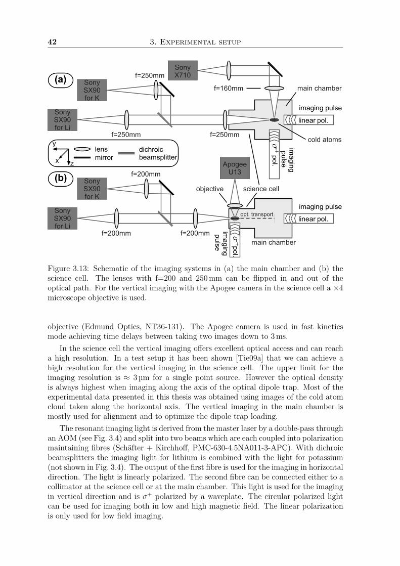
42 3. Experimental setup
SonySX90for Li
SonySX90for K
f=200mm
f=200mmf=200mm
imaging pulse
linear pol.
SonySX90for Li
SonySX90for K
SonyX710f=250mm
f=250mm f=250mm
f=160mm
lensmirror
dichroicbeamsplitter
z
y
x ApogeeU13
imaging pulse
linear pol.s+
pol.
opt. transport
main chamber
science cell
imaging
pulse
imaging
pulse
main chamber(a)
(b)objective
cold atoms
s+pol.
Figure 3.13: Schematic of the imaging systems in (a) the main chamber and (b) thescience cell. The lenses with f=200 and 250mm can be flipped in and out of theoptical path. For the vertical imaging with the Apogee camera in the science cell a ×4microscope objective is used.
objective (Edmund Optics, NT36-131). The Apogee camera is used in fast kineticsmode achieving time delays between taking two images down to 3ms.
In the science cell the vertical imaging offers excellent optical access and can reacha high resolution. In a test setup it has been shown [Tie09a] that we can achieve ahigh resolution for the vertical imaging in the science cell. The upper limit for theimaging resolution is ≈ 3 µm for a single point source. However the optical densityis always highest when imaging along the axis of the optical dipole trap. Most of theexperimental data presented in this thesis was obtained using images of the cold atomcloud taken along the horizontal axis. The vertical imaging in the main chamber ismostly used for alignment and to optimize the dipole trap loading.
The resonant imaging light is derived from the master laser by a double-pass throughan AOM (see Fig. 3.4) and split into two beams which are each coupled into polarizationmaintaining fibres (Schäfter + Kirchhoff, PMC-630-4.5NA011-3-APC). With dichroicbeamsplitters the imaging light for lithium is combined with the light for potassium(not shown in Fig. 3.4). The output of the first fibre is used for the imaging in horizontaldirection. The light is linearly polarized. The second fibre can be connected either to acollimator at the science cell or at the main chamber. This light is used for the imagingin vertical direction and is σ+ polarized by a waveplate. The circular polarized lightcan be used for imaging both in low and high magnetic field. The linear polarizationis only used for low field imaging.

3.8. Imaging systems 43
3.8.2 Fluorescence imagingFor florescence imaging in the main chamber we irradiate the atoms with near resonantlight using the MOT beams and the light scatters in all directions. The MOT beamsare under an angle to the imaging path, so only scattered photons and no photons ofthe MOT beams are detected by the CCD camera. A trapped atom in the MOT canscatter many photons without being lost from the trap. This allows for long exposuretimes of the camera and thus a good signal to noise ratio. This imaging method is usedto characterise the MOT, the magnetic trap and to optimize the magnetic trap captureefficiency. We only used it for relative measurements, which do not require calibrationof the signal. The characterization of the lithium 2D-MOT-source in [Tie09b] was alsodone using fluorescence imaging.
3.8.3 Absorption imagingFor absorption imaging a low intensity resonant light pulse passes through the cloudof atoms onto the camera. In areas where there are atoms, the light is absorbed andthe image shows a shadow of the atomic sample. In this thesis all absorption imageswere taken after release of the atoms from a trap after variable times of expansion. Inballistic expansion only a few photons can be scattered per atom as atomic motion andphoton recoil can blur the image. In addition to the resonant light a pulse of repumplight is switched on when imaging to prevent a population of dark states. In the mainchamber the repump light is part of the MOT beams, therefore under a 45 angle to theimaging beam and in two counter-propagating beams. In the science cell the repumplight is back reflected and under an angle of ≈ 30 to the imaging path. During theimaging pulse the atoms absorb photons from the imaging beam and re-scatter themin all directions. For a resonant light pulse of duration ∆t with low intensity, i.e. thesaturation parameter s0 = I/Is 1, the number of photons Np scattered is given byNp = 1
2s0Γ∆t, with Γ being the natural linewidth of the optical transition [Met99].The recoil from the absorbed photons shifts the atoms out of resonance due to theDoppler effect. The frequency shift is given by ωD = vreckNp, with the wavevector kof the light and the recoil velocity vrec = ~k/m. The re-emission moves the atoms inrandom directions resulting in a blurring of the cloud’s image. The atoms are thenon average displaced in the transverse direction by rrms = vrec∆t
√Np/3 [Jof93]. For
potassium we use intensities for the imaging pulses with saturation parameter s0 = 0.4and a pulse length of ∆t = 100 µs, resulting in a displacement by rrms = 9 µm and afrequency shift of ωD = 0.4Γ.
To obtain a signal from the CCD camera three images need to be recorded. Afterevery absorption image taken with intensity Iabs, two images of the optical field aretaken. One as a reference with imaging light Iref and one without imaging light withintensity Ibg as background. The signal is then: I(x, y)/I0(x, y) = (Iabs − Ibg)/(Iref −Ibg). For the Sony cameras we found that the background image Ibg can be neglected,and it is not used in the analysis of the data. The intensity distribution is used tocalculate the column density of the atomic distribution using the Lambert-Beer law:
I(x, y)I0(x, y) = exp(−OD) = exp(−σn(x, y)),
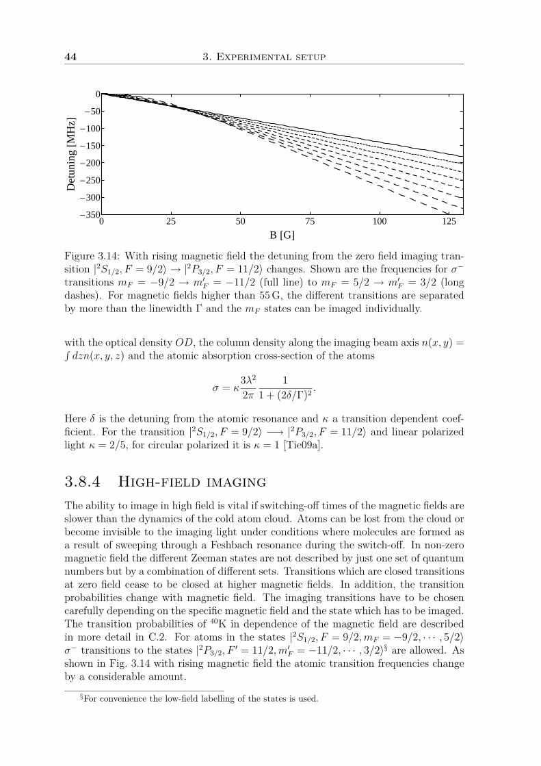
44 3. Experimental setup
0 25 50 75 100 125-350
-300
-250
-200
-150
-100
-50
0
B @GD
Det
unin
g@M
HzD
Figure 3.14: With rising magnetic field the detuning from the zero field imaging tran-sition |2S1/2, F = 9/2〉 → |2P3/2, F = 11/2〉 changes. Shown are the frequencies for σ−transitions mF = −9/2 → m′F = −11/2 (full line) to mF = 5/2 → m′F = 3/2 (longdashes). For magnetic fields higher than 55G, the different transitions are separatedby more than the linewidth Γ and the mF states can be imaged individually.
with the optical density OD, the column density along the imaging beam axis n(x, y) =∫dzn(x, y, z) and the atomic absorption cross-section of the atoms
σ = κ3λ2
2π1
1 + (2δ/Γ)2 .
Here δ is the detuning from the atomic resonance and κ a transition dependent coef-ficient. For the transition |2S1/2, F = 9/2〉 −→ |2P3/2, F = 11/2〉 and linear polarizedlight κ = 2/5, for circular polarized it is κ = 1 [Tie09a].
3.8.4 High-field imagingThe ability to image in high field is vital if switching-off times of the magnetic fields areslower than the dynamics of the cold atom cloud. Atoms can be lost from the cloud orbecome invisible to the imaging light under conditions where molecules are formed asa result of sweeping through a Feshbach resonance during the switch-off. In non-zeromagnetic field the different Zeeman states are not described by just one set of quantumnumbers but by a combination of different sets. Transitions which are closed transitionsat zero field cease to be closed at higher magnetic fields. In addition, the transitionprobabilities change with magnetic field. The imaging transitions have to be chosencarefully depending on the specific magnetic field and the state which has to be imaged.The transition probabilities of 40K in dependence of the magnetic field are describedin more detail in C.2. For atoms in the states |2S1/2, F = 9/2,mF = −9/2, · · · , 5/2〉σ− transitions to the states |2P3/2, F
′ = 11/2,m′F = −11/2, · · · , 3/2〉§ are allowed. Asshown in Fig. 3.14 with rising magnetic field the atomic transition frequencies changeby a considerable amount.
§For convenience the low-field labelling of the states is used.
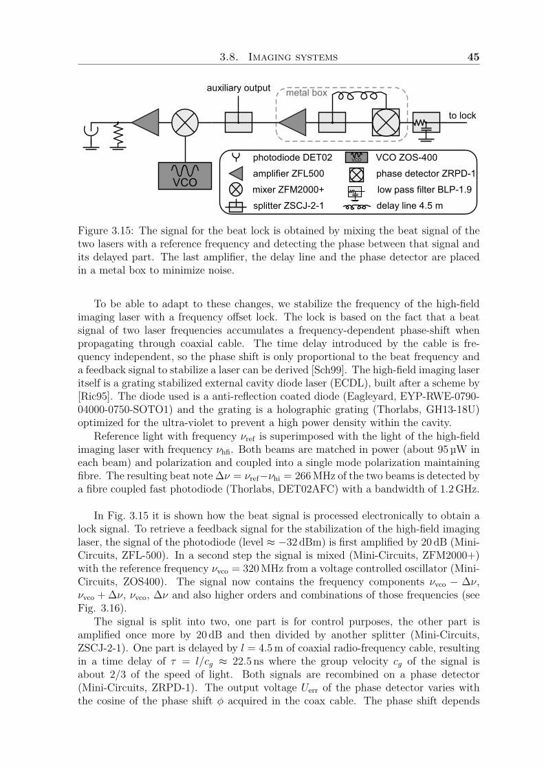
3.8. Imaging systems 45
photodiode DET02
VCOamplifier ZFL500
mixer ZFM2000+
splitter ZSCJ-2-1
VCO
delay line 4.5 m
VCO ZOS-400
phase detector ZRPD-1
low pass filter BLP-1.9
auxiliary output
to lock
metal box
Figure 3.15: The signal for the beat lock is obtained by mixing the beat signal of thetwo lasers with a reference frequency and detecting the phase between that signal andits delayed part. The last amplifier, the delay line and the phase detector are placedin a metal box to minimize noise.
To be able to adapt to these changes, we stabilize the frequency of the high-fieldimaging laser with a frequency offset lock. The lock is based on the fact that a beatsignal of two laser frequencies accumulates a frequency-dependent phase-shift whenpropagating through coaxial cable. The time delay introduced by the cable is fre-quency independent, so the phase shift is only proportional to the beat frequency anda feedback signal to stabilize a laser can be derived [Sch99]. The high-field imaging laseritself is a grating stabilized external cavity diode laser (ECDL), built after a scheme by[Ric95]. The diode used is a anti-reflection coated diode (Eagleyard, EYP-RWE-0790-04000-0750-SOTO1) and the grating is a holographic grating (Thorlabs, GH13-18U)optimized for the ultra-violet to prevent a high power density within the cavity.
Reference light with frequency νref is superimposed with the light of the high-fieldimaging laser with frequency νhfi. Both beams are matched in power (about 95µW ineach beam) and polarization and coupled into a single mode polarization maintainingfibre. The resulting beat note ∆ν = νref−νhi = 266MHz of the two beams is detected bya fibre coupled fast photodiode (Thorlabs, DET02AFC) with a bandwidth of 1.2GHz.
In Fig. 3.15 it is shown how the beat signal is processed electronically to obtain alock signal. To retrieve a feedback signal for the stabilization of the high-field imaginglaser, the signal of the photodiode (level ≈ −32dBm) is first amplified by 20 dB (Mini-Circuits, ZFL-500). In a second step the signal is mixed (Mini-Circuits, ZFM2000+)with the reference frequency νvco = 320MHz from a voltage controlled oscillator (Mini-Circuits, ZOS400). The signal now contains the frequency components νvco − ∆ν,νvco + ∆ν, νvco, ∆ν and also higher orders and combinations of those frequencies (seeFig. 3.16).
The signal is split into two, one part is for control purposes, the other part isamplified once more by 20 dB and then divided by another splitter (Mini-Circuits,ZSCJ-2-1). One part is delayed by l = 4.5m of coaxial radio-frequency cable, resultingin a time delay of τ = l/cg ≈ 22.5 ns where the group velocity cg of the signal isabout 2/3 of the speed of light. Both signals are recombined on a phase detector(Mini-Circuits, ZRPD-1). The output voltage Uerr of the phase detector varies withthe cosine of the phase shift φ acquired in the coax cable. The phase shift depends
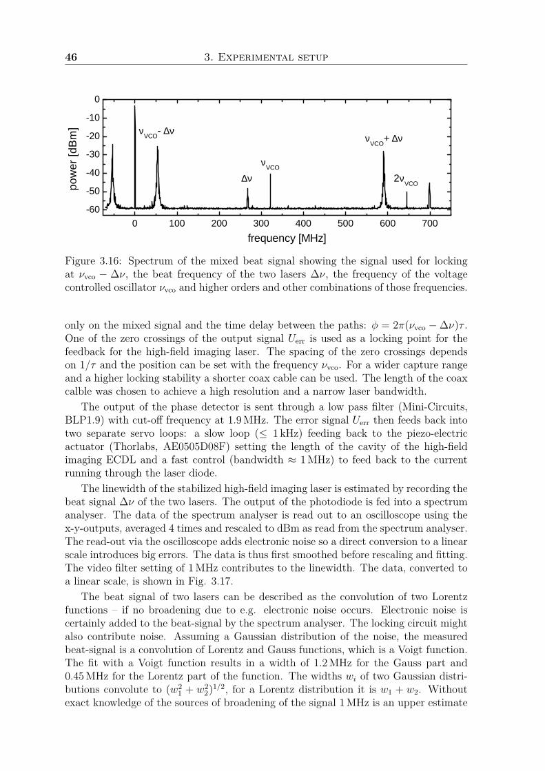
46 3. Experimental setup
0 1 0 0 2 0 0 3 0 0 4 0 0 5 0 0 6 0 0 7 0 0- 6 0- 5 0- 4 0- 3 0- 2 0- 1 0
0
2 ν V C O
ν V C O + ∆ν
ν V C O∆ν
ν V C O - ∆ν
f r e q u e n c y [ M H z ]
powe
r [dBm
]
Figure 3.16: Spectrum of the mixed beat signal showing the signal used for lockingat νvco − ∆ν, the beat frequency of the two lasers ∆ν, the frequency of the voltagecontrolled oscillator νvco and higher orders and other combinations of those frequencies.
only on the mixed signal and the time delay between the paths: φ = 2π(νvco −∆ν)τ .One of the zero crossings of the output signal Uerr is used as a locking point for thefeedback for the high-field imaging laser. The spacing of the zero crossings dependson 1/τ and the position can be set with the frequency νvco. For a wider capture rangeand a higher locking stability a shorter coax cable can be used. The length of the coaxcalble was chosen to achieve a high resolution and a narrow laser bandwidth.
The output of the phase detector is sent through a low pass filter (Mini-Circuits,BLP1.9) with cut-off frequency at 1.9MHz. The error signal Uerr then feeds back intotwo separate servo loops: a slow loop (≤ 1 kHz) feeding back to the piezo-electricactuator (Thorlabs, AE0505D08F) setting the length of the cavity of the high-fieldimaging ECDL and a fast control (bandwidth ≈ 1MHz) to feed back to the currentrunning through the laser diode.
The linewidth of the stabilized high-field imaging laser is estimated by recording thebeat signal ∆ν of the two lasers. The output of the photodiode is fed into a spectrumanalyser. The data of the spectrum analyser is read out to an oscilloscope using thex-y-outputs, averaged 4 times and rescaled to dBm as read from the spectrum analyser.The read-out via the oscilloscope adds electronic noise so a direct conversion to a linearscale introduces big errors. The data is thus first smoothed before rescaling and fitting.The video filter setting of 1MHz contributes to the linewidth. The data, converted toa linear scale, is shown in Fig. 3.17.
The beat signal of two lasers can be described as the convolution of two Lorentzfunctions – if no broadening due to e.g. electronic noise occurs. Electronic noise iscertainly added to the beat-signal by the spectrum analyser. The locking circuit mightalso contribute noise. Assuming a Gaussian distribution of the noise, the measuredbeat-signal is a convolution of Lorentz and Gauss functions, which is a Voigt function.The fit with a Voigt function results in a width of 1.2MHz for the Gauss part and0.45MHz for the Lorentz part of the function. The widths wi of two Gaussian distri-butions convolute to (w2
1 + w22)1/2, for a Lorentz distribution it is w1 + w2. Without
exact knowledge of the sources of broadening of the signal 1MHz is an upper estimate
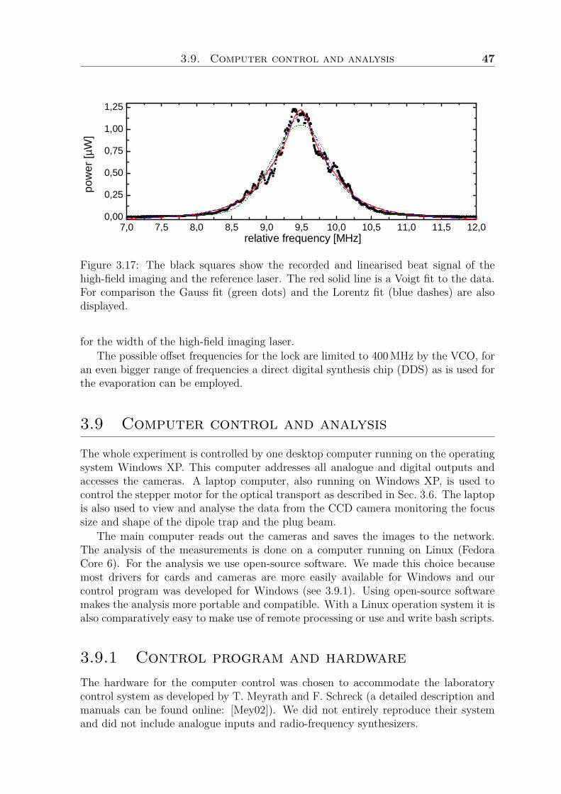
3.9. Computer control and analysis 47
7 , 0 7 , 5 8 , 0 8 , 5 9 , 0 9 , 5 1 0 , 0 1 0 , 5 1 1 , 0 1 1 , 5 1 2 , 00 , 0 00 , 2 50 , 5 00 , 7 51 , 0 01 , 2 5
r e l a t i v e f r e q u e n c y [ M H z ]
powe
r [µW]
Figure 3.17: The black squares show the recorded and linearised beat signal of thehigh-field imaging and the reference laser. The red solid line is a Voigt fit to the data.For comparison the Gauss fit (green dots) and the Lorentz fit (blue dashes) are alsodisplayed.
for the width of the high-field imaging laser.The possible offset frequencies for the lock are limited to 400MHz by the VCO, for
an even bigger range of frequencies a direct digital synthesis chip (DDS) as is used forthe evaporation can be employed.
3.9 Computer control and analysis
The whole experiment is controlled by one desktop computer running on the operatingsystem Windows XP. This computer addresses all analogue and digital outputs andaccesses the cameras. A laptop computer, also running on Windows XP, is used tocontrol the stepper motor for the optical transport as described in Sec. 3.6. The laptopis also used to view and analyse the data from the CCD camera monitoring the focussize and shape of the dipole trap and the plug beam.
The main computer reads out the cameras and saves the images to the network.The analysis of the measurements is done on a computer running on Linux (FedoraCore 6). For the analysis we use open-source software. We made this choice becausemost drivers for cards and cameras are more easily available for Windows and ourcontrol program was developed for Windows (see 3.9.1). Using open-source softwaremakes the analysis more portable and compatible. With a Linux operation system it isalso comparatively easy to make use of remote processing or use and write bash scripts.
3.9.1 Control program and hardwareThe hardware for the computer control was chosen to accommodate the laboratorycontrol system as developed by T. Meyrath and F. Schreck (a detailed description andmanuals can be found online: [Mey02]). We did not entirely reproduce their systemand did not include analogue inputs and radio-frequency synthesizers.
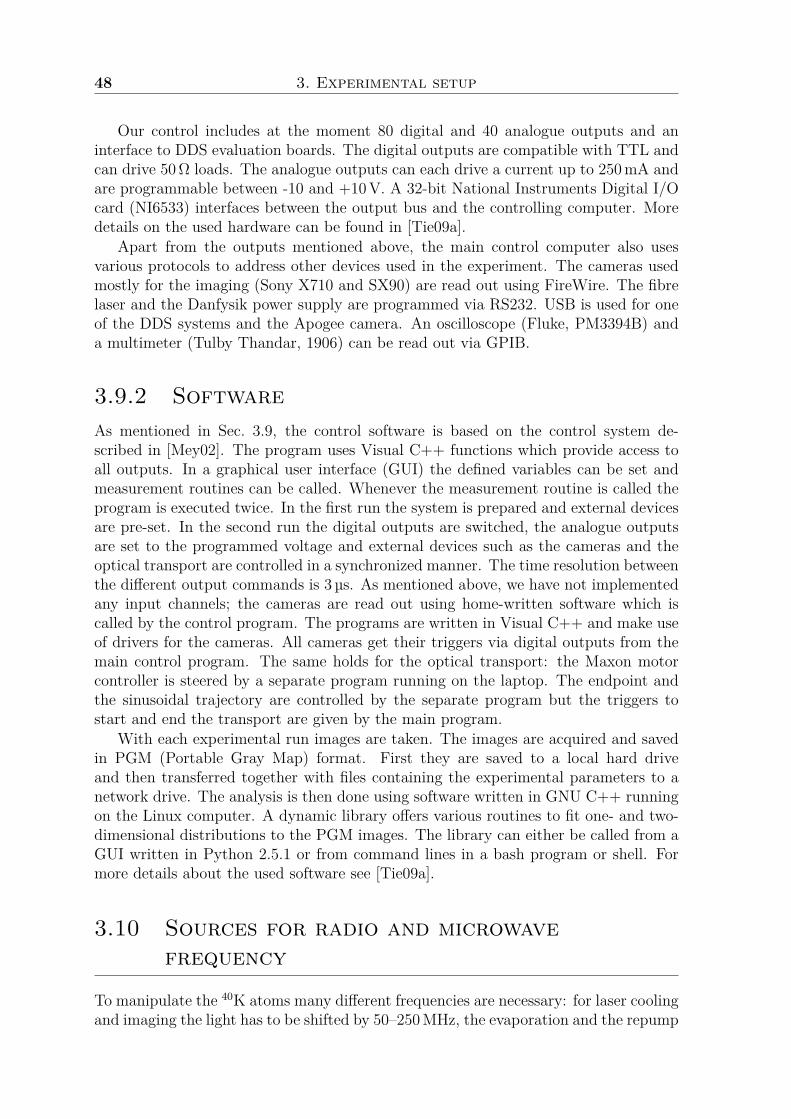
48 3. Experimental setup
Our control includes at the moment 80 digital and 40 analogue outputs and aninterface to DDS evaluation boards. The digital outputs are compatible with TTL andcan drive 50Ω loads. The analogue outputs can each drive a current up to 250mA andare programmable between -10 and +10V. A 32-bit National Instruments Digital I/Ocard (NI6533) interfaces between the output bus and the controlling computer. Moredetails on the used hardware can be found in [Tie09a].
Apart from the outputs mentioned above, the main control computer also usesvarious protocols to address other devices used in the experiment. The cameras usedmostly for the imaging (Sony X710 and SX90) are read out using FireWire. The fibrelaser and the Danfysik power supply are programmed via RS232. USB is used for oneof the DDS systems and the Apogee camera. An oscilloscope (Fluke, PM3394B) anda multimeter (Tulby Thandar, 1906) can be read out via GPIB.
3.9.2 SoftwareAs mentioned in Sec. 3.9, the control software is based on the control system de-scribed in [Mey02]. The program uses Visual C++ functions which provide access toall outputs. In a graphical user interface (GUI) the defined variables can be set andmeasurement routines can be called. Whenever the measurement routine is called theprogram is executed twice. In the first run the system is prepared and external devicesare pre-set. In the second run the digital outputs are switched, the analogue outputsare set to the programmed voltage and external devices such as the cameras and theoptical transport are controlled in a synchronized manner. The time resolution betweenthe different output commands is 3 µs. As mentioned above, we have not implementedany input channels; the cameras are read out using home-written software which iscalled by the control program. The programs are written in Visual C++ and make useof drivers for the cameras. All cameras get their triggers via digital outputs from themain control program. The same holds for the optical transport: the Maxon motorcontroller is steered by a separate program running on the laptop. The endpoint andthe sinusoidal trajectory are controlled by the separate program but the triggers tostart and end the transport are given by the main program.
With each experimental run images are taken. The images are acquired and savedin PGM (Portable Gray Map) format. First they are saved to a local hard driveand then transferred together with files containing the experimental parameters to anetwork drive. The analysis is then done using software written in GNU C++ runningon the Linux computer. A dynamic library offers various routines to fit one- and two-dimensional distributions to the PGM images. The library can either be called from aGUI written in Python 2.5.1 or from command lines in a bash program or shell. Formore details about the used software see [Tie09a].
3.10 Sources for radio and microwavefrequency
To manipulate the 40K atoms many different frequencies are necessary: for laser coolingand imaging the light has to be shifted by 50–250MHz, the evaporation and the repump
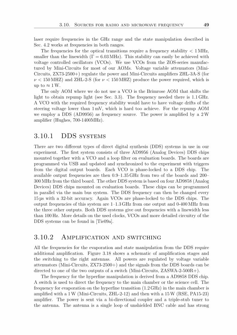
3.10. Sources for radio and microwave frequency 49
laser require frequencies in the GHz range and the state manipulation described inSec. 4.2 works at frequencies in both ranges.
The frequencies for the optical transitions require a frequency stability < 1MHz,smaller than the linewidth (Γ = 6.03MHz). This stability can easily be achieved withvoltage controlled oscillators (VCOs). We use VCOs from the ZOS-series manufac-tured by Mini-Circuits for most of our AOMs. Voltage variable attenuators (Mini-Circuits, ZX73-2500+) regulate the power and Mini-Circuits amplifiers ZHL-3A-S (forν < 150MHZ) and ZHL-2-S (for ν < 150MHZ) produce the power required, which isup to ≈ 1W.
The only AOM where we do not use a VCO is the Brimrose AOM that shifts thelight to obtain repump light (see Sec. 3.3). The frequency needed there is 1.1GHz.A VCO with the required frequency stability would have to have voltage drifts of thesteering voltage lower than 1mV, which is hard too achieve. For the repump AOMwe employ a DDS (AD9956) as frequency source. The power is amplified by a 2Wamplifier (Hughes, 700-1400MHz).
3.10.1 DDS systemsThere are two different types of direct digital synthesis (DDS) systems in use in ourexperiment. The first system consists of three AD9956 (Analog Devices) DDS chipsmounted together with a VCO and a loop filter on evaluation boards. The boards areprogrammed via USB and updated and synchronized to the experiment with triggersfrom the digital output boards. Each VCO is phase-locked to a DDS chip. Theavailable output frequencies are then 0.9–1.35GHz from two of the boards and 200–300MHz from the third board. The other DDS system is based on four AD9858 (AnalogDevices) DDS chips mounted on evaluation boards. These chips can be programmedin parallel via the main bus system. The DDS frequency can then be changed every15µs with a 32-bit accuracy. Again VCOs are phase-locked to the DDS chips. Theoutput frequencies of this system are 1–1.3GHz from one output and 0-400MHz fromthe three other outputs. Both DDS systems give out frequencies with a linewidth lessthan 100Hz. More details on the used clocks, VCOs and more detailed circuitry of theDDS systems can be found in [Tie09a].
3.10.2 Amplification and switchingAll the frequencies for the evaporation and state manipulation from the DDS requireadditional amplification. Figure 3.18 shows a schematic of amplification stages andthe switching to the right antennas. All powers are regulated by voltage variableattenuators (Mini-Circuits, ZX73-2500+) and the signals from the DDS boards can bedirected to one of the two outputs of a switch (Mini-Circuits, ZASWA-2-500R+).
The frequency for the hyperfine manipulation is derived from a AD9858 DDS chip.A switch is used to direct the frequency to the main chamber or the science cell. Thefrequency for evaporation on the hyperfine transition (1.2GHz) in the main chamber isamplified with a 1W (Mini-Circuits, ZHL-2-12) and then with a 15W (RSE, PA15-23)amplifier. The power is sent via a bi-directional coupler and a triple-stub tuner tothe antenna. The antenna is a single loop of unshielded BNC cable and has strong
50 3. Experimental setup
relay
amplifier*ZHL-2-12
circulator
DDS AD98580 - 400 MHz
amplifier*ZX60-3018G
amplifier*TIA-1000-1R8
amplifierPA15-23 (RSE)
amplifier2330PATV(Downeast)
switc
h*ZA
SW
A-2
-500
R VVatt*ZX73-2500
VVatt*ZX73-2500
VVatt*ZX73-2500
switc
h*ZA
SW
A-2
-500
R
DDS AD98581 - 1.3 GHz
coupler
evaporation
mainchamber
main chamber
sciencecell
science cell
calibration/clean outantenna
state preparation/calibration
Figure 3.18: Schematic of the amplification stages for the radio and microwave frequen-cies used to manipulate the atoms. All components marked with * are manufacturedby Mini-Circuits. The triple-stub tuner is omitted from the schematic.
resonances. The triple-stub tuner is tuned to achieve a flat frequency response in therange 1.1–1.3GHz.
When the other output of the switch is in use, the microwave power is increasedfirst by 12.8 dB (Mini-Circuits, ZX60-3018G) and then sent through a 30W (Downeast,2330PATV) amplifier and a circulator to the antenna. In the science cell this frequencyrange is used for the clean out of undesired Zeeman states and for the calibration of themagnetic field as described in Chapter 4. The bi-directional coupler and the circulatorprotect the amplifiers from the power being reflected back by the antenna.
The lower frequency range from 0–400MHz is used for the preparation of the properZeeman states and for field calibration in the science cell. Here the output from theAD9858 DDS chip can be switched to a 50Ω terminator to prevent noise. For boththe use in the main chamber and the science cell the radio frequency is amplified bythe same 4W (Mini-Circuits,TIA-1000-R18) amplifier. The switching between the twoantennas is done with a relay. There is no circulator or coupler in this path as theamplifier is protected against back-reflected power.
The antennas for the radio and microwave frequencies consist of simple wire loops.The antennas for the microwave have one winding and the ones for the radio frequencyhave seven. For more detailed specifications of the used antennas and the setup for thelithium antennas see Table 3.3 in [Tie09a].

Chapter 4
Experimental sequence
In this chapter a description is given of the preparation of ultracold atoms in the desiredZeeman states and the measurements of Feshbach resonances in collisions betweenatoms. Figure 4.1 shows an overview of the entire experimental sequence in the formof a timeline. The sequence displayed is used for most measurements of Feshbachresonances, the cases where the procedure is adapted are described in the text. Thepreparation of the cold atoms involves evaporation steps and a transport of the coldsample to the science cell, where the Zeeman states are prepared and the measurementsare taken. Each experimental cycle takes up to 60 s, depending on the holding timeat a specific magnetic field to determine magnetic field dependent losses. Furthermorethe magnetic field calibration and selected measurements are presented.
A vital step in the experimental sequence is the reproducible preparation of binarymixtures of Zeeman states. This is required to be able to investigate a Feshbachresonance in a specific channel. Multi component mixtures of Zeeman states complicatethe assignment of observed loss features.
In earlier experiments on the apparatus [Tie09a] a number of different state prepara-tion procedures were implemented in the main chamber. The 40K atoms were preparedin the fully stretched |F = 9/2,mF = 9/2〉 state by forced evaporation of the unde-sired states in the magnetic trap or in a combination of optical and magnetic trap.Additionally optical transitions at low and high magnetic field and adiabatic sweepsto high-field seeking states were employed. All these experiments made use of Zeemanstate sensitive detection by means of a Stern-Gerlach experiment in the main chamber.However, the Stern-Gerlach detection in the main chamber required very low dipoletrap frequencies ωr = 2π× 560Hz (corresponding to about 2% of the full ODT power)to resolve the individual states to confirm a succesful state preparation. At such lowODT powers a lossless optical transport of the cold clouds to the science cell can hardlybe achieved, the ODT is best set to full power for this purpose. In the absence of statedependent detection the preparation of the states at a higher trap depth can leaveatoms in undesired states undetected. In addition, without Stern-Gerlach experimentat the science cell, de-polarization of the states during the transport is difficult todetect.
In the course of this work we build a coil to perform Stern-Gerlach detection (seeSec. 3.7) at the science cell. We added switches and antennas (see Sec. 3.10.2) to have
52 4. Experimental sequence
MO
Tloading
16s
MO
Tcom
-pression
10m
s
Feshbachexperim
ent
-2D-MO
Toff
-shimcoilsoff
-MO
Toff
-offsetB-field
on-opt.pum
pinglighton
60ms
MT
com-
pression
-MT
on
evaporation
300m
s22.3
s
-plugoff
-B-offseton
250m
s4.4
s
opticaltransport
3s
evaporationstate
cleaning
140m
s
rftransfers
1s510m
s
opticalpum
pingO
DT
loading
0.5-10
s
-B-offsethigher
-FB-coilson
-FB-coiloff
-gradienton
-ODT
off
Stern-G
erlachim
aging
-Bfields
off
-2D-MO
Ton
-3D-MO
Ton
-plugon-O
DTon
-MT
off-B-offsethigher
|B|
OD
Tpow
er
time
(nottoscale)
detectionopticaldipole
trap(O
DT)
opt.pum
pingm
agnetictrap
(MT)
MO
T
sciencecell
main
chamber
AB
CD
EF
GH
IJ
KL
MN
delay
transport
Figure4.1:
Simplified
schematic
oftheexperim
entalsequence.The
lowergraph
showsthe
appliedmagnetic
fieldsand
thepower
ofthe
ODT.In
thetext
theexperim
entalstepsA
toN
aredescribed
indetail.
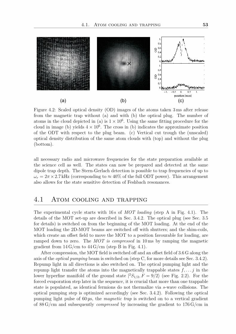
4.1. Atom cooling and trapping 53
(a) (b) (c)
Figure 4.2: Scaled optical density (OD) images of the atoms taken 3ms after releasefrom the magnetic trap without (a) and with (b) the optical plug. The number ofatoms in the cloud depicted in (a) is 1× 10⁶. Using the same fitting procedure for thecloud in image (b) yields 4× 10⁶. The cross in (b) indicates the approximate positionof the ODT with respect to the plug beam. (c) Vertical cut trough the (unscaled)optical density distribution of the same atom clouds with (top) and without the plug(bottom).
all necessary radio and microwave frequencies for the state preparation available atthe science cell as well. The states can now be prepared and detected at the samedipole trap depth. The Stern-Gerlach detection is possible to trap frequencies of up toωr = 2π×2.7 kHz (corresponding to ≈ 40% of the full ODT power). This arrangementalso allows for the state sensitive detection of Feshbach resonances.
4.1 Atom cooling and trapping
The experimental cycle starts with 16 s of MOT loading (step A in Fig. 4.1). Thedetails of the MOT set-up are described in Sec. 3.4.2. The optical plug (see Sec. 3.5for details) is switched on from the beginning of the MOT loading. At the end of theMOT loading the 2D-MOT beams are switched off with shutters; and the shim-coils,which create an offset field to move the MOT to a position favourable for loading, areramped down to zero. The MOT is compressed in 10ms by ramping the magneticgradient from 14G/cm to 44G/cm (step B in Fig. 4.1).
After compression, the MOT field is switched off and an offset field of 3.6G along theaxis of the optical pumping beam is switched on (step C, for more details see Sec. 3.4.2).Repump light in all directions is also switched on. The optical pumping light and therepump light transfer the atoms into the magnetically trappable states f, . . . j in thelower hyperfine manifold of the ground state |2S1/2, F = 9/2〉 (see Fig. 2.2). For theforced evaporation step later in the sequence, it is crucial that more than one trappablestate is populated, as identical fermions do not thermalize via s-wave collisions. Theoptical pumping step is optimized accordingly (see Sec. 3.4.2). Following the opticalpumping light pulse of 60µs, the magnetic trap is switched on to a vertical gradientof 88G/cm and subsequently compressed by increasing the gradient to 176G/cm in
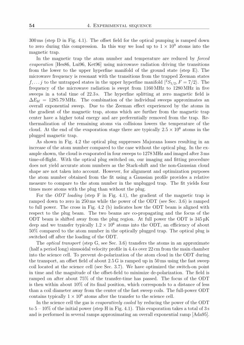
54 4. Experimental sequence
300ms (step D in Fig. 4.1). The offset field for the optical pumping is ramped downto zero during this compression. In this way we load up to 1 × 10⁹ atoms into themagnetic trap.
In the magnetic trap the atom number and temperature are reduced by forcedevaporation [Hes86, Lui96, Ket96] using microwave radiation driving the transitionsfrom the lower to the upper hyperfine manifold of the ground state (step E). Themicrowave frequency is resonant with the transitions from the trapped Zeeman statesf, . . . j to the untrapped states in the upper hyperfine manifold |2S1/2, F = 7/2〉. Thefrequency of the microwave radiation is swept from 1160MHz to 1280MHz in fivesweeps in a total time of 22.3 s. The hyperfine splitting at zero magnetic field is∆Ehf = 1285.79MHz. The combination of the individual sweeps approximates anoverall exponential sweep. Due to the Zeeman effect experienced by the atoms inthe gradient of the magnetic trap, atoms which are further from the magnetic trapcenter have a higher total energy and are preferentially removed from the trap. Re-thermalization of the remaining atoms via collisions lowers the temperature of thecloud. At the end of the evaporation stage there are typically 2.5 × 10⁶ atoms in theplugged magnetic trap.
As shown in Fig. 4.2 the optical plug suppresses Majorana losses resulting in anincrease of the atom number compared to the case without the optical plug. In the ex-ample shown, the cloud is evaporated in four sweeps to 1278MHz and imaged after 3mstime-of-flight. With the optical plug switched on, our imaging and fitting proceduredoes not yield accurate atom numbers as the Stark-shift and the non-Gaussian cloudshape are not taken into account. However, for alignment and optimization purposesthe atom number obtained from the fit using a Gaussian profile provides a relativemeasure to compare to the atom number in the unplugged trap. The fit yields fourtimes more atoms with the plug than without the plug.
For the ODT loading (step F in Fig. 4.1), the gradient of the magnetic trap isramped down to zero in 250ms while the power of the ODT (see Sec. 3.6) is rampedto full power. The cross in Fig. 4.2 (b) indicates how the ODT beam is aligned withrespect to the plug beam. The two beams are co-propagating and the focus of theODT beam is shifted away from the plug region. At full power the ODT is 345µKdeep and we transfer typically 1.2 × 10⁶ atoms into the ODT, an efficiency of about50% compared to the atom number in the optically plugged trap. The optical plug isswitched off after the loading of the ODT.
The optical transport (step G, see Sec. 3.6) transfers the atoms in an approximate(half a period long) sinusoidal velocity profile in 4.4 s over 22 cm from the main chamberinto the science cell. To prevent de-polarization of the atom cloud in the ODT duringthe transport, an offset field of about 2.5G is ramped up in 50ms using the fast sweepcoil located at the science cell (see Sec. 3.7). We have optimized the switch-on pointin time and the magnitude of the offset-field to minimize de-polarization. The field isramped on after about 75% of the transfer-time has passed. The focus of the ODTis then within about 10% of its final position, which corresponds to a distance of lessthan a coil diameter away from the center of the fast sweep coils. The full-power ODTcontains typically 1× 10⁶ atoms after the transfer to the science cell.
In the science cell the gas is evaporatively cooled by reducing the power of the ODTto 5 – 10% of the initial power (step H in Fig. 4.1). This evaporation takes a total of 3 sand is performed in several ramps approximating an overall exponential ramp [Ada95].
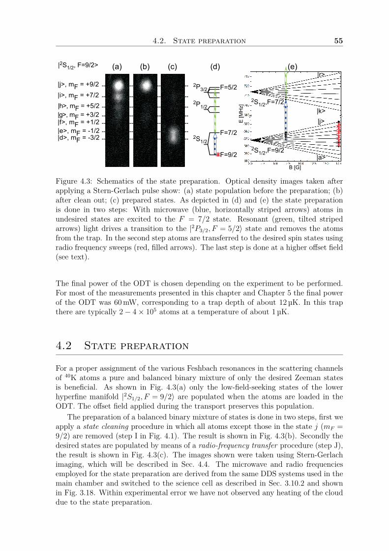
4.2. State preparation 55
2S1/2,F=9/2
2S1/2,F=7/2
|a>
|j>
B [G]
(e)
E[M
Hz]
|j>, mF = +9/2|i>, mF = +7/2|h>, mF = +5/2|g>, mF = +3/2|f>, mF = +1/2|e>, mF = -1/2|d>, mF = -3/2
|2S1/2, F=9/2> (a) (b) (c)
2S1/2
2P1/2
2P3/2
F=9/2
F=7/2
F=5/2
(d)
|k>
|r>
Figure 4.3: Schematics of the state preparation. Optical density images taken afterapplying a Stern-Gerlach pulse show: (a) state population before the preparation; (b)after clean out; (c) prepared states. As depicted in (d) and (e) the state preparationis done in two steps: With microwave (blue, horizontally striped arrows) atoms inundesired states are excited to the F = 7/2 state. Resonant (green, tilted stripedarrows) light drives a transition to the |2P3/2, F = 5/2〉 state and removes the atomsfrom the trap. In the second step atoms are transferred to the desired spin states usingradio frequency sweeps (red, filled arrows). The last step is done at a higher offset field(see text).
The final power of the ODT is chosen depending on the experiment to be performed.For most of the measurements presented in this chapter and Chapter 5 the final powerof the ODT was 60mW, corresponding to a trap depth of about 12 µK. In this trapthere are typically 2− 4× 10⁵ atoms at a temperature of about 1 µK.
4.2 State preparation
For a proper assignment of the various Feshbach resonances in the scattering channelsof 40K atoms a pure and balanced binary mixture of only the desired Zeeman statesis beneficial. As shown in Fig. 4.3(a) only the low-field-seeking states of the lowerhyperfine manifold |2S1/2, F = 9/2〉 are populated when the atoms are loaded in theODT. The offset field applied during the transport preserves this population.
The preparation of a balanced binary mixture of states is done in two steps, first weapply a state cleaning procedure in which all atoms except those in the state j (mF =9/2) are removed (step I in Fig. 4.1). The result is shown in Fig. 4.3(b). Secondly thedesired states are populated by means of a radio-frequency transfer procedure (step J),the result is shown in Fig. 4.3(c). The images shown were taken using Stern-Gerlachimaging, which will be described in Sec. 4.4. The microwave and radio frequenciesemployed for the state preparation are derived from the same DDS systems used in themain chamber and switched to the science cell as described in Sec. 3.10.2 and shownin Fig. 3.18. Within experimental error we have not observed any heating of the clouddue to the state preparation.

56 4. Experimental sequence
1268 1270 1272 1274 1276 1278 12801
2
3
45
Figure 4.4: Loss features in the atom number when driving the labelled transitionswithout applying atom removal light. The offset field in this example is about 6G andthe frequency is scanned for each point over 300 kHz in 300ms.
4.2.1 State cleaningThe state cleaning procedure is illustrated in Fig. 4.3(d) and (e). The atoms in theundesired Zeeman states f, g, h, i in the lower hyperfine manifold |2S1/2, F = 9/2〉 areexcited with microwave radiation to the upper manifold |2S1/2, F = 7/2〉. From therethe atoms are removed by resonant σ−-polarized light tuned to the |2S1/2, F = 7/2〉 −→|2P3/2, F = 5/2〉 electronic transition in the D2-line.
The atom removal light is necessary due to spin exchange. To illustrate the phe-nomenology, we show in Fig. 4.4 the effect of microwave sweeps in the range of 1268–1280MHz. In this example the sweeps are done without atom removal light. For eachpoint the frequency is swept over 300 kHz in 300ms. Loss features appear when thefrequency is resonant with transitions to the upper hyperfine manifold. The loss oc-curs because atoms excited to the upper hyperfine manifold undergo spin exchangingcollisions [Hap72] with the atoms in the lower hyperfine manifold, resulting in atomloss. Contrary to spin exchange within the lower hyperfine manifold (see Sec. 2.4)this process is exothermic, releasing energy in the mK range, heating the atom cloudsto temperatures higher than the trap depth of the ODT. As expected for this spin-exchange mechanism, the loss of the population also occurs in states which are notexcited by the microwave radiation. This is shown in Fig. 4.5, where the atoms aredetected with Stern-Gerlach imaging.
The state cleaning for the Feshbach measurements is done in the science cell at anoffset field of 7.2G produced by the fast sweep coils in the presence of atom removallight. The field is ramped up in 50ms from the offset value used during the transport.With a series of four sweeps of microwave radiation the atoms from the undesired statesf, g, h, i in the lower hyperfine manifold are excited to the states k, l,m, n in the upperhyperfine manifold. In each of the four sweeps, the microwave radiation is swept overa range of 50 kHz in 35ms. These sweeps are done around the frequencies to drive
4.2. State preparation 57
1265 1266 1267 1268 1269 1270 1271 1272 1273 1274 1275 12760.00
0.05
0.10
0.15
0.20 mF = 9/2 , j mF = 7/2 , i mF = 5/2 , h mF = 3/2 , g mF = 1/2 , f
frequency [MHz]
atom
numb
er [a
rb. u
.]
Figure 4.5: Loss in spin states due to spin exchanging collisions with states in the upperhyperfine manifold when not applying atom removal light. Around 1271MHz only thej → k microwave transition is driven. At 1274.6MHz only the transitions i → l andh→ k are addressed. The offset field in this example is about 6G.
the transitions g → n and f → m (first sweep); h → l (second sweep); i → l andh→ k (third sweep); and i→ k (fourth sweep). The atom removal light tuned to the|2S1/2, F = 7/2〉 −→ |2P3/2, F = 5/2〉 transition prevents losses due to spin exchangebetween the microwave excited atoms and the remaining atoms in the states in thelower hyperfine manifold. At the offset field employed, the Zeeman splitting of thefour populated states in the upper manifold is about 6MHz, the same as the linewidthΓ of the D2 line. The Zeeman splitting of the electronically excited states in the|2P3/2, F = 5/2〉 manifold at the offset field is about 2Γ. With sufficient intensity, itis not necessary to sweep the frequency of the atom removal light, but adequate totune the frequency within about 2Γ for optimal atom removal. The intensity anddetuning of the atom removal light is optimized by exciting the population of one ofthe trapped states by microwave radiation to the upper hyperfine manifold, applyingatom removal light and detecting the remaining atoms with Stern-Gerlach imaging.When the atoms are efficiently removed from the upper hyperfine manifold, no lossesoccur in the remaining trapped states. The population in the cleaned-out state isminimized, while the occupation in the other states is conserved. When the intensityof the atom removal light is too high, also atoms in the lower hyperfine manifold areoptically excited to the |2P3/2〉 manifold and are lost from the sample. The optimalintensity was established experimentally.
4.2.2 State transfersThe state cleaning leaves atoms only in the |2S1/2 F = 9/2,mF = 9/2〉 state. For a70mW deep trap, the atom number is typically 1.7 × 10⁵. From there the atoms aretransferred in two radio-frequency sweeps [Rub81] to the desired final states. To geta good resolution between the states, the offset field is increased from 7.2G to about
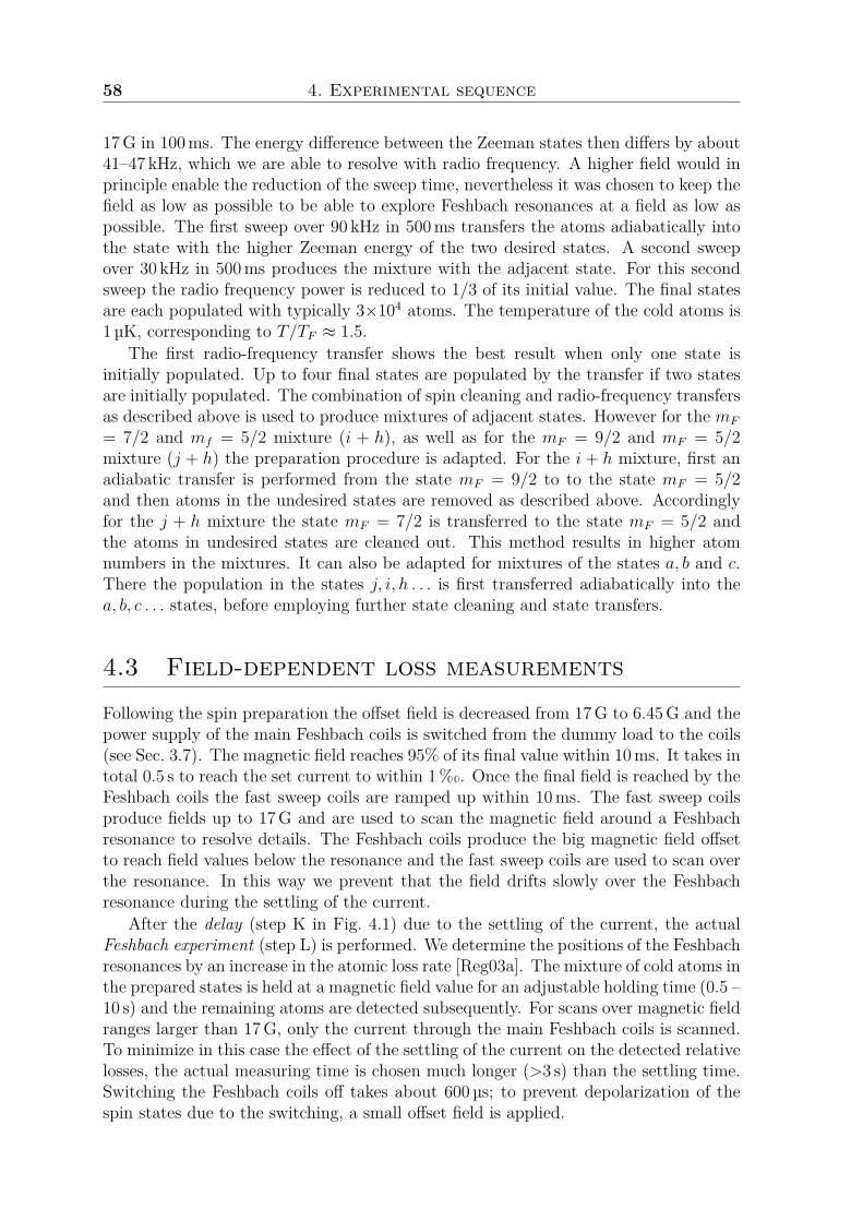
58 4. Experimental sequence
17G in 100ms. The energy difference between the Zeeman states then differs by about41–47 kHz, which we are able to resolve with radio frequency. A higher field would inprinciple enable the reduction of the sweep time, nevertheless it was chosen to keep thefield as low as possible to be able to explore Feshbach resonances at a field as low aspossible. The first sweep over 90 kHz in 500ms transfers the atoms adiabatically intothe state with the higher Zeeman energy of the two desired states. A second sweepover 30 kHz in 500ms produces the mixture with the adjacent state. For this secondsweep the radio frequency power is reduced to 1/3 of its initial value. The final statesare each populated with typically 3×10⁴ atoms. The temperature of the cold atoms is1 µK, corresponding to T/TF ≈ 1.5.
The first radio-frequency transfer shows the best result when only one state isinitially populated. Up to four final states are populated by the transfer if two statesare initially populated. The combination of spin cleaning and radio-frequency transfersas described above is used to produce mixtures of adjacent states. However for the mF
= 7/2 and mf = 5/2 mixture (i + h), as well as for the mF = 9/2 and mF = 5/2mixture (j + h) the preparation procedure is adapted. For the i + h mixture, first anadiabatic transfer is performed from the state mF = 9/2 to to the state mF = 5/2and then atoms in the undesired states are removed as described above. Accordinglyfor the j + h mixture the state mF = 7/2 is transferred to the state mF = 5/2 andthe atoms in undesired states are cleaned out. This method results in higher atomnumbers in the mixtures. It can also be adapted for mixtures of the states a, b and c.There the population in the states j, i, h . . . is first transferred adiabatically into thea, b, c . . . states, before employing further state cleaning and state transfers.
4.3 Field-dependent loss measurements
Following the spin preparation the offset field is decreased from 17G to 6.45G and thepower supply of the main Feshbach coils is switched from the dummy load to the coils(see Sec. 3.7). The magnetic field reaches 95% of its final value within 10ms. It takes intotal 0.5 s to reach the set current to within 1%. Once the final field is reached by theFeshbach coils the fast sweep coils are ramped up within 10ms. The fast sweep coilsproduce fields up to 17G and are used to scan the magnetic field around a Feshbachresonance to resolve details. The Feshbach coils produce the big magnetic field offsetto reach field values below the resonance and the fast sweep coils are used to scan overthe resonance. In this way we prevent that the field drifts slowly over the Feshbachresonance during the settling of the current.
After the delay (step K in Fig. 4.1) due to the settling of the current, the actualFeshbach experiment (step L) is performed. We determine the positions of the Feshbachresonances by an increase in the atomic loss rate [Reg03a]. The mixture of cold atoms inthe prepared states is held at a magnetic field value for an adjustable holding time (0.5 –10 s) and the remaining atoms are detected subsequently. For scans over magnetic fieldranges larger than 17G, only the current through the main Feshbach coils is scanned.To minimize in this case the effect of the settling of the current on the detected relativelosses, the actual measuring time is chosen much longer (>3 s) than the settling time.Switching the Feshbach coils off takes about 600 µs; to prevent depolarization of thespin states due to the switching, a small offset field is applied.
4.4. Stern-Gerlach imaging 59
4.4 Stern-Gerlach imagingOnce the Feshbach coils are switched off, the mixture is detected by absorption imagingafter a time-of-flight. To distinguish the different spin states contained in the cold atomcloud a Stern-Gerlach gradient field (step M in Fig. 4.1) is applied before zero-fieldimaging (step N in Fig. 4.1). The magnetic gradient is pulsed on for the first 3.7msof the time-of-flight after the cold atoms are released from the optical dipole trap. Asingle coil, situated about 1 cm above the atom cloud, produces a gradient of 100G/cm,which is sufficient to separate the spin states during the 4ms total time-of-flight. Thecurrent is switched between a resistive dummy load and the coil using FETs. Thisensures a fast switching of the Stern-Gerlach field. Again, to prevent depolarization ofthe states during the switching, an offset field of 6.45G is applied.
After all the coils are switched off and the magnetic field has decayed, the imag-ing and repump light flashes are applied and the atoms in the separated clouds aredetected. The switch-off of the offset field does not affect the state-dependent detec-tion, as the initial population distribution in the states spin is now separated in space.Any depolarization at this stage is not relevant, the imaging itself is done without anapplied field (see Sec. 3.8).
The Stern-Gerlach pulse is sufficient to separate the spin states in clouds at tem-peratures of around 12µK, so it is necessary to evaporate from the ODT to a trapdepth of at most 140 µK. This trap depth corresponds to 40% of the full power ofthe ODT and results in a trap frequency of ωr = 2π × 2.7 kHz. Compared to theStern-Gerlach detection previously implemented in the main chamber [Tie09a], this isa major improvement.
A separation of the spin states of clouds at even higher temperatures could beachieved with a higher magnetic field gradient. In the restricted available space thiscould be done by using two coils, but then the separation of the states is impeded asthe atoms get partially trapped.
4.5 Magnetic field calibrationThe magnetic field is calibrated by driving the transitions either between the twoground state hyperfine manifolds or between Zeeman states within the lower hyperfinemanifold. For the frequencies required the corresponding magnetic field is calculatedusing the Breit-Rabi formula as described in Appendix B.1. We calibrate the fieldduring the measurement part of the sequence (see Sec. 4.3).
The choice of the transition employed for the calibration depends on the frequencyranges available from the DDS system (see Sec. 3.10.1). The DDS system deliverseither radio frequency radiation in the range 0 – 400MHz or microwave frequencyradiation in the range 1 – 1.3GHz. In the case of high magnetic fields the transitionbetween the Zeeman states |2S1/2, F = 9/2,mF = 9/2〉 and |2S1/2, F = 9/2,mF = 7/2〉is driven with radio frequency. The calibration is done by detecting the populationin the mF = 7/2 state versus the frequency. An example for the calibration withradio frequency is shown in Fig. 4.6(b). For low field the hyperfine transition between|2S1/2, F = 9/2,mF = 9/2〉 and |2S1/2, F = 7/2,mF = 7/2〉 is driven and the loss inthe |F = 9/2,mF = 9/2〉 state is detected with changing frequency. In both cases the
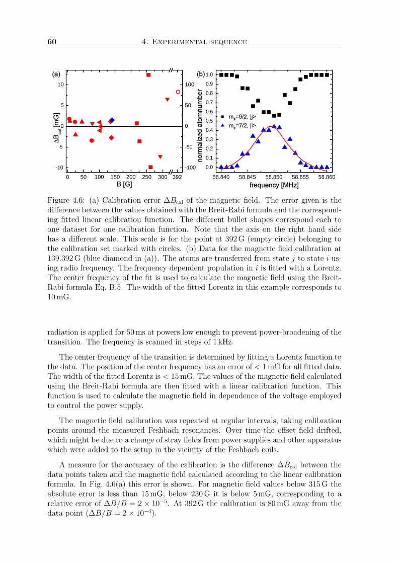
60 4. Experimental sequence
0 50 100 150 200 250 300 392-10
-5
0
5
10
-100
-50
0
50
100
58.840 58.845 58.850 58.855 58.8600.00.10.20.30.40.50.60.70.80.91.0
Figure 4.6: (a) Calibration error ∆Bcal of the magnetic field. The error given is thedifference between the values obtained with the Breit-Rabi formula and the correspond-ing fitted linear calibration function. The different bullet shapes correspond each toone dataset for one calibration function. Note that the axis on the right hand sidehas a different scale. This scale is for the point at 392G (empty circle) belonging tothe calibration set marked with circles. (b) Data for the magnetic field calibration at139.392G (blue diamond in (a)). The atoms are transferred from state j to state i us-ing radio frequency. The frequency dependent population in i is fitted with a Lorentz.The center frequency of the fit is used to calculate the magnetic field using the Breit-Rabi formula Eq. B.5. The width of the fitted Lorentz in this example corresponds to10mG.
radiation is applied for 50ms at powers low enough to prevent power-broadening of thetransition. The frequency is scanned in steps of 1 kHz.
The center frequency of the transition is determined by fitting a Lorentz function tothe data. The position of the center frequency has an error of < 1mG for all fitted data.The width of the fitted Lorentz is < 15mG. The values of the magnetic field calculatedusing the Breit-Rabi formula are then fitted with a linear calibration function. Thisfunction is used to calculate the magnetic field in dependence of the voltage employedto control the power supply.
The magnetic field calibration was repeated at regular intervals, taking calibrationpoints around the measured Feshbach resonances. Over time the offset field drifted,which might be due to a change of stray fields from power supplies and other apparatuswhich were added to the setup in the vicinity of the Feshbach coils.
A measure for the accuracy of the calibration is the difference ∆Bcal between thedata points taken and the magnetic field calculated according to the linear calibrationformula. In Fig. 4.6(a) this error is shown. For magnetic field values below 315G theabsolute error is less than 15mG, below 230G it is below 5mG, corresponding to arelative error of ∆B/B = 2 × 10⁻⁵. At 392G the calibration is 80mG away from thedata point (∆B/B = 2× 10⁻⁴).
4.5. Magnetic field calibration 61
Limits to the magnetic field precisionThe stability of the power supply for the Feshbach coils (see Sec. 3.7) is specified to<1ppm, so the precision of the measured magnetic field is likely to be limited byother factors. The current running through the coil gives rise to heating and thermalexpansion, which lowers the magnetic field for a given current. For a linear thermalexpansion of the coil, the relative change in magnetic field is ∆B/B = −1.7× 10⁻⁵/K.At high currents (28.5A corresponding to 500G), the temperature of the coils rises onlyslowly by 3C with a time-constant of 4min as described in [Tie09a]. The maximumtemperature of the coil is constant to within 0.1K for a period of two hours. This islimited by the temperature drift of the cooling water which runs through the mount ata pressure of 2 bar. The temperature of the cooling water also shows day to day driftsof 0.5K. During the experimental cycle, the coil is on for at most 11 s the temperatureincreases in this time by approximately 0.082K, resulting in ∆B/B < −1.4 × 10⁻⁶.When including the delay time due to the settling of the current and considering atypical measuring time of 4 s the relative change in magnetic field is at most−4.3×10⁻⁷.This shows that in principal a very high accuracy can be achieved with the Feshbachcoil and the employed power supply. The thermal stability of the Feshbach coil is notlimiting the measured magnetic field precision.
The only part of the Feshbach coil circuit which was not optimized for thermalstability when taking the data presented in this thesis, is the MOSFET switch. TheMOSFETs are likely to be responsible for the observed loss in magnetic field precisionat large magnetic fields. The MOSFETs are mounted on heat sinks and are not activelycooled. Running a high current through the MOSFETs leads to considerable heating(up to 20C) within the measuring time. The drain – source resistance of a MOSFETrises non-linearly with temperature and current. For a higher current the effect is moresevere and can lead to a runaway behaviour which ultimately destroys the MOSFET.The 20C rise in temperature increases the resistance by a factor 1.5, however theDanfysik power supply is not specified to regulate such big load changes. After theswitch from the dummy load to the coil the current takes 0.5 s to settle within 1%†. Itis specified to regulate up to 10% resistance changes within <0.05 ppm. Recently theMOSFET switch has been equipped with water-cooling, so the change in resistance ofthe MOSFETs should be below 10% and we should be able to eliminate the switch asa cause for the loss in accuracy.
A limiting factor for the magnetic field precision, which we could not test yet,can be short term fluctuations of the background magnetic field originating from theelectrical equipment running at 50Hz of the main power line. The background is notin phase with the experimental cycle and contributes to a varying offset. To improvethe magnetic field stability in the future, the experimental cycle could be synchronizedto the 50Hz frequency of the main power line. This would suppress common noise inthe offset magnetic field which can influence the precision of the state preparation andcalibration. With the synchronization it would also be possible to test the long-termstability of the magnetic field.
Another cause for the lower limit of the measured magnetic field precision can†To measure the current running through the Feshbach coils we use a Agilent (N2775A, 50MHz)
current probe. The current is limited to 15A, corresponding to a field of about 260G. The resolutionis about 20mA corresponding to 350mG (1%).
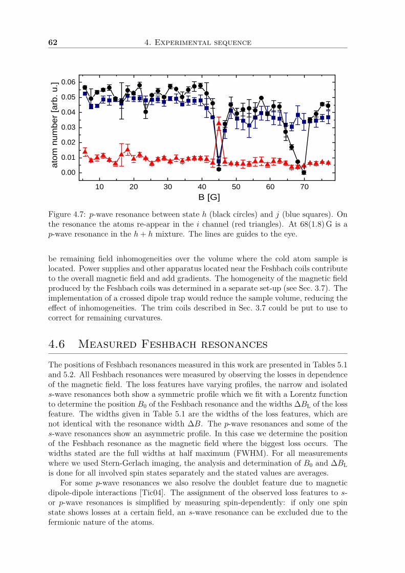
62 4. Experimental sequence
10 20 30 40 50 60 700.000.010.020.030.040.050.06
B [G]
atom
numb
er [a
rb. u
.]
Figure 4.7: p-wave resonance between state h (black circles) and j (blue squares). Onthe resonance the atoms re-appear in the i channel (red triangles). At 68(1.8)G is ap-wave resonance in the h+ h mixture. The lines are guides to the eye.
be remaining field inhomogeneities over the volume where the cold atom sample islocated. Power supplies and other apparatus located near the Feshbach coils contributeto the overall magnetic field and add gradients. The homogeneity of the magnetic fieldproduced by the Feshbach coils was determined in a separate set-up (see Sec. 3.7). Theimplementation of a crossed dipole trap would reduce the sample volume, reducing theeffect of inhomogeneities. The trim coils described in Sec. 3.7 could be put to use tocorrect for remaining curvatures.
4.6 Measured Feshbach resonancesThe positions of Feshbach resonances measured in this work are presented in Tables 5.1and 5.2. All Feshbach resonances were measured by observing the losses in dependenceof the magnetic field. The loss features have varying profiles, the narrow and isolateds-wave resonances both show a symmetric profile which we fit with a Lorentz functionto determine the position B0 of the Feshbach resonance and the widths ∆BL of the lossfeature. The widths given in Table 5.1 are the widths of the loss features, which arenot identical with the resonance width ∆B. The p-wave resonances and some of thes-wave resonances show an asymmetric profile. In this case we determine the positionof the Feshbach resonance as the magnetic field where the biggest loss occurs. Thewidths stated are the full widths at half maximum (FWHM). For all measurementswhere we used Stern-Gerlach imaging, the analysis and determination of B0 and ∆BLis done for all involved spin states separately and the stated values are averages.
For some p-wave resonances we also resolve the doublet feature due to magneticdipole-dipole interactions [Tic04]. The assignment of the observed loss features to s-or p-wave resonances is simplified by measuring spin-dependently: if only one spinstate shows losses at a certain field, an s-wave resonance can be excluded due to thefermionic nature of the atoms.
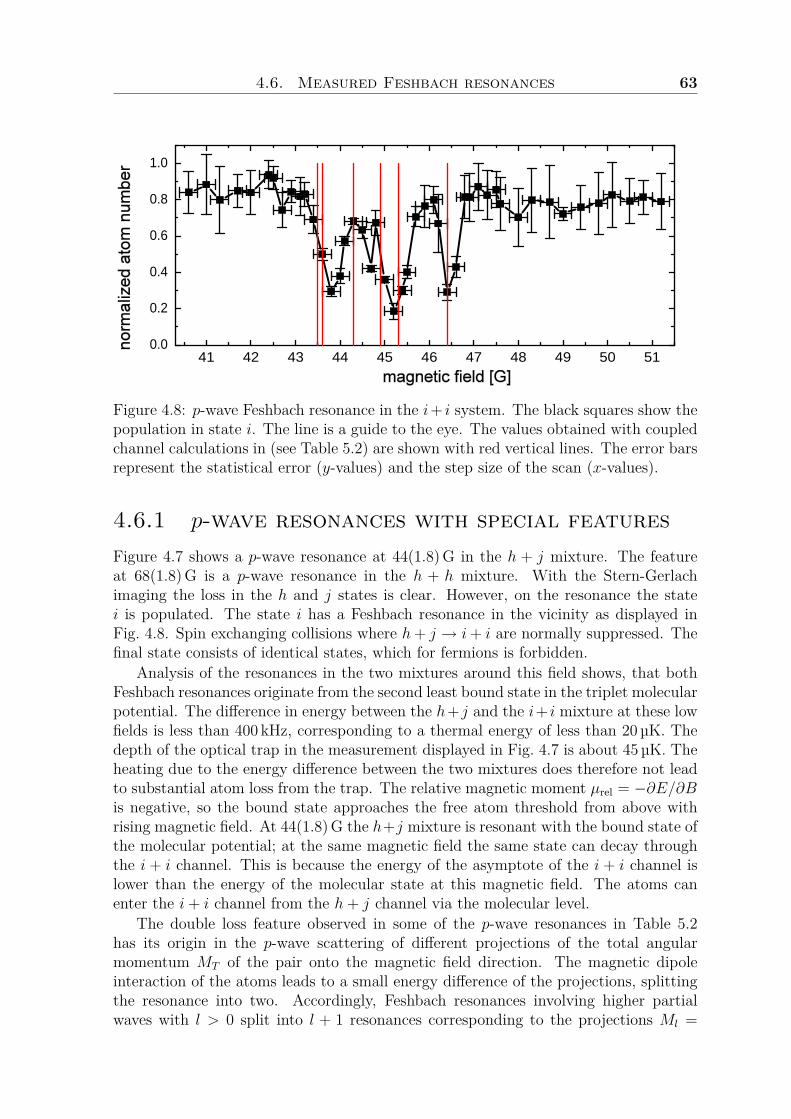
4.6. Measured Feshbach resonances 63
41 42 43 44 45 46 47 48 49 50 510.0
0.2
0.4
0.6
0.8
1.0
Figure 4.8: p-wave Feshbach resonance in the i+ i system. The black squares show thepopulation in state i. The line is a guide to the eye. The values obtained with coupledchannel calculations in (see Table 5.2) are shown with red vertical lines. The error barsrepresent the statistical error (y-values) and the step size of the scan (x-values).
4.6.1 p-wave resonances with special featuresFigure 4.7 shows a p-wave resonance at 44(1.8)G in the h + j mixture. The featureat 68(1.8)G is a p-wave resonance in the h + h mixture. With the Stern-Gerlachimaging the loss in the h and j states is clear. However, on the resonance the statei is populated. The state i has a Feshbach resonance in the vicinity as displayed inFig. 4.8. Spin exchanging collisions where h+ j → i+ i are normally suppressed. Thefinal state consists of identical states, which for fermions is forbidden.
Analysis of the resonances in the two mixtures around this field shows, that bothFeshbach resonances originate from the second least bound state in the triplet molecularpotential. The difference in energy between the h+ j and the i+ i mixture at these lowfields is less than 400 kHz, corresponding to a thermal energy of less than 20µK. Thedepth of the optical trap in the measurement displayed in Fig. 4.7 is about 45µK. Theheating due to the energy difference between the two mixtures does therefore not leadto substantial atom loss from the trap. The relative magnetic moment µrel = −∂E/∂Bis negative, so the bound state approaches the free atom threshold from above withrising magnetic field. At 44(1.8)G the h+j mixture is resonant with the bound state ofthe molecular potential; at the same magnetic field the same state can decay throughthe i + i channel. This is because the energy of the asymptote of the i + i channel islower than the energy of the molecular state at this magnetic field. The atoms canenter the i+ i channel from the h+ j channel via the molecular level.
The double loss feature observed in some of the p-wave resonances in Table 5.2has its origin in the p-wave scattering of different projections of the total angularmomentum MT of the pair onto the magnetic field direction. The magnetic dipoleinteraction of the atoms leads to a small energy difference of the projections, splittingthe resonance into two. Accordingly, Feshbach resonances involving higher partialwaves with l > 0 split into l + 1 resonances corresponding to the projections Ml =
64 4. Experimental sequence
0, |±1|, |±2|, . . . |±l|. This feature is thermally broadened and therefore only detectablewhen the temperature of the atoms is lower than the splitting [Tic04].
The multiplet structure in Fig. 4.8 in the i+ i mixture was measured at a temper-ature of about 3µK. It is not only a double but a quadruple feature, which is causedby the coupling of channels due to dipole-dipole interaction. The i+ i channel couplesto the i+ j, h+ i and h+ h channel and depending on the projections of Ml on thesechannels Feshbach resonances occur at different magnetic fields. The values obtainedwith coupled channel calculations (see Sec. 5.3.1) are shown as vertical lines in Fig. 4.8.
When forming molecules at a p-wave resonance, the projections of the total angularmomentum is visible in the angular distribution of the dissociated molecules as demon-strated by [Gae07]. P -wave resonances, where the magnetic dipole interaction splitsthe resonance into two distinct resonances, have been proposed to tune anisotropicinteraction between atoms [Tic04, Bar02].
4.6.2 Width of a Feshbach resonanceApart from the exact position of a Feshbach resonance it is also important to determineits width. The width has influence on the resonance strength (see Sec. 2.5) and onthe requirements for the magnetic field stability. The width of the loss feature ∆BL
is affected by more parameters than the resonance width alone and gives therefore noquantitative information on the resonance width. To determine the width of a Feshbachresonance the effect of scattering properties of the cold cloud can be measured. Weevaporate the cold atom cloud around the Feshbach resonance in the c + d mixtureat 178.3G and detect the size of the cloud after evaporation in dependence of themagnetic field.
For the measurement described in this section the experimental sequence as de-scribed above is slightly altered. The evaporation in the optical dipole trap is done intwo steps. At first the power of the ODT is ramped down exponentially from full powerto 150mW in 600ms. At this trap depth the atoms are prepared in a c + d mixturewith the method described in Sec. 4.2. Then the Feshbach coils are switched on andonce the final field is reached, a second evaporation step follows. In 5 s the power isreduced to 20mW in an exponential ramp. After another 200ms at the final field thecold atom cloud is imaged at zero field without the Stern-Gerlach pulse after 3.5mstime-of-flight. The data points in Fig. 4.9 show the cloud size in the radial directionof the ODT.
When evaporating the cold atom cloud around a Feshbach resonance the scatteringcross section σ changes with magnetic field. As a result the final atom number andtemperature of the cloud differ, for small σ the evaporation is less efficient and thecloud is hotter and bigger and vice versa. Just below the resonance the cloud is heatedby 3-body losses due to the molecular state present and the cloud size is increased. Thetwo data points, where this occurs (shown as squares in Fig. 4.9) have been omitted inthe fit described below.
We fit the data using an approximative model. The behaviour of the cloud sizeS(B) with varying magnetic field is attributed to the behaviour of the scattering crosssection σ over the resonance (see Sec. 2.3). The maximum cloud size S0 is assumed tooccur at the zero crossing of the scattering length Ba=0 = B0 + ∆B and the minimalvalue at the resonance position B0. During the evaporation ramp, the depth of the
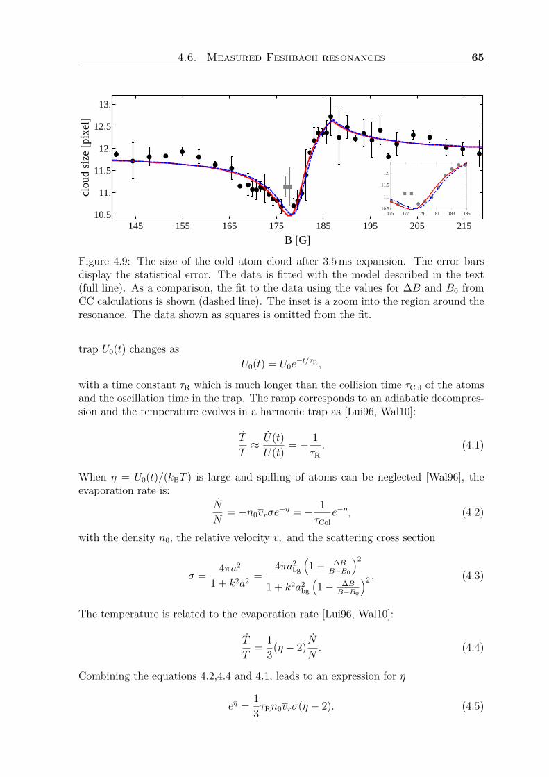
4.6. Measured Feshbach resonances 65
æ
ææ æ
ææ
ææ
æ æææ
æææ
ææ
æ ææ
æ
æ
æ
æ
æææ
æ
æ
æ
ææ
æ
æ
æ
æ
æ æ
æ ææ
àà
145 155 165 175 185 195 205 21510.5
11.
11.5
12.
12.5
13.
B @GD
clou
dsi
ze@pi
xelD
ææ
æ ææ
ææ
æ
æ ææ æ æ æ
ææ æ
æ ææ
æ
æ
æ
ææ æ æ
æ
à à
175 177 179 181 183 18510.5
11.
11.5
12.
Figure 4.9: The size of the cold atom cloud after 3.5ms expansion. The error barsdisplay the statistical error. The data is fitted with the model described in the text(full line). As a comparison, the fit to the data using the values for ∆B and B0 fromCC calculations is shown (dashed line). The inset is a zoom into the region around theresonance. The data shown as squares is omitted from the fit.
trap U0(t) changes asU0(t) = U0e
−t/τR ,
with a time constant τR which is much longer than the collision time τCol of the atomsand the oscillation time in the trap. The ramp corresponds to an adiabatic decompres-sion and the temperature evolves in a harmonic trap as [Lui96, Wal10]:
T
T≈ U(t)U(t) = − 1
τR. (4.1)
When η = U0(t)/(kBT ) is large and spilling of atoms can be neglected [Wal96], theevaporation rate is:
N
N= −n0vrσe
−η = − 1τCol
e−η, (4.2)
with the density n0, the relative velocity vr and the scattering cross section
σ = 4πa2
1 + k2a2 =4πa2
bg
(1− ∆B
B−B0
)2
1 + k2a2bg
(1− ∆B
B−B0
)2 . (4.3)
The temperature is related to the evaporation rate [Lui96, Wal10]:
T
T= 1
3(η − 2)NN. (4.4)
Combining the equations 4.2,4.4 and 4.1, leads to an expression for η
eη = 13τRn0vrσ(η − 2). (4.5)
66 4. Experimental sequence
This equation can be solved with the Lambert W(x) function (product logarithm)[NIS11, Sco06, Wit11]. For equations of the form
e−cu = a(u− b),
where a, b, c ∈ R, it is
u = b+ 1cW(ce
−cb
a).
Using this result we obtain:
η = 2−W(−3e2
τRn0vrσ
)= 2−W
(−3e2τCol
τR
). (4.6)
For |x| < 1/e the Lambert W(x) function can be written as a power series
W(x) = x− x2 + · · · .
For a ramping time constant τR τCol the condition is fulfilled and the expression forη takes the form:
η ≈ 2 + const.× σ−1. (4.7)
The cloud size after expansion is described in a harmonic approximation (see Eq. A.12and [Gri00]) by:
S ∝ 1√η. (4.8)
The final size Sf of the cloud after evaporation is the initial size Si ∝√kBTi/Ui reduced
by a value depending on the field dependent behaviour of η during the evaporation:
Sf = Si −∆S(η(B)).
At the zero crossing of the resonance, where σ = 0, the cloud will not thermalize. Inthe experiments the initial η is rather large (≈ 10), so we assume that spilling of atomsonly plays a minor role [Wal96] and that the size of cloud S0 for σ = 0 is determinedby the initial temperature Ti and the final potential depth Uf as: S0 =
√Ui/Uf Si.
The field dependent size of the cloud can then be described as
Sf ∝ S0
1− 1√η(B)
.Replacing η(B) with the expression for η in Eq. 4.7, and rearranging the expression weobtain as a fitting function for the measured cloud size:
S(B) = S0
1−
P 21
(1− ∆B
B−B0
)2
1 + P 22
(1− ∆B
B−B0
)2
1/2 , (4.9)
where the width ∆B and the position B0 of the resonance and the maximum cloud sizeS0 are fitting parameters. The fitting parameters P1 and P2 incorporate the effect of
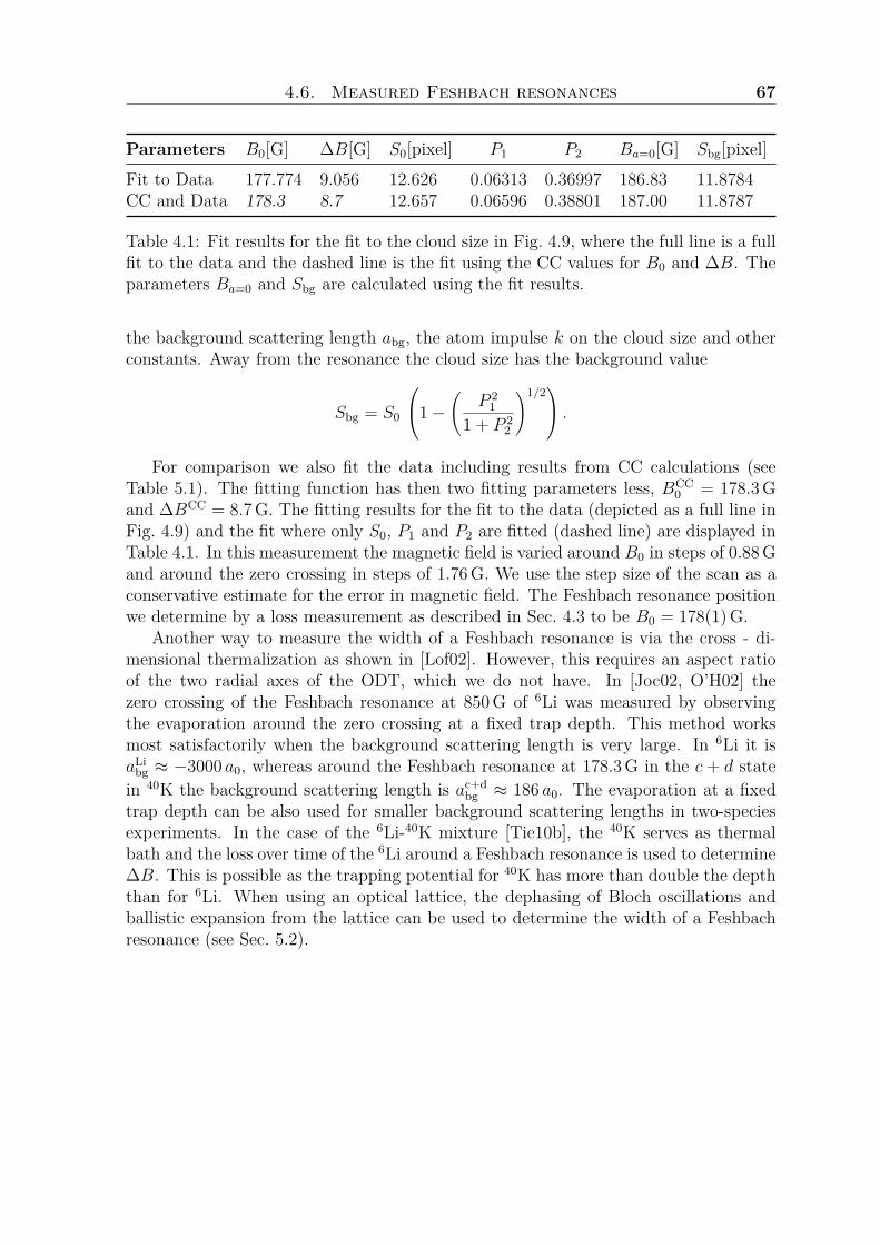
4.6. Measured Feshbach resonances 67
Parameters B0[G] ∆B[G] S0[pixel] P1 P2 Ba=0[G] Sbg[pixel]Fit to Data 177.774 9.056 12.626 0.06313 0.36997 186.83 11.8784CC and Data 178.3 8.7 12.657 0.06596 0.38801 187.00 11.8787
Table 4.1: Fit results for the fit to the cloud size in Fig. 4.9, where the full line is a fullfit to the data and the dashed line is the fit using the CC values for B0 and ∆B. Theparameters Ba=0 and Sbg are calculated using the fit results.
the background scattering length abg, the atom impulse k on the cloud size and otherconstants. Away from the resonance the cloud size has the background value
Sbg = S0
1−(
P 21
1 + P 22
)1/2 .
For comparison we also fit the data including results from CC calculations (seeTable 5.1). The fitting function has then two fitting parameters less, BCC
0 = 178.3Gand ∆BCC = 8.7G. The fitting results for the fit to the data (depicted as a full line inFig. 4.9) and the fit where only S0, P1 and P2 are fitted (dashed line) are displayed inTable 4.1. In this measurement the magnetic field is varied around B0 in steps of 0.88Gand around the zero crossing in steps of 1.76G. We use the step size of the scan as aconservative estimate for the error in magnetic field. The Feshbach resonance positionwe determine by a loss measurement as described in Sec. 4.3 to be B0 = 178(1)G.
Another way to measure the width of a Feshbach resonance is via the cross - di-mensional thermalization as shown in [Lof02]. However, this requires an aspect ratioof the two radial axes of the ODT, which we do not have. In [Joc02, O’H02] thezero crossing of the Feshbach resonance at 850G of 6Li was measured by observingthe evaporation around the zero crossing at a fixed trap depth. This method worksmost satisfactorily when the background scattering length is very large. In 6Li it isaLi
bg ≈ −3000 a0, whereas around the Feshbach resonance at 178.3G in the c + d statein 40K the background scattering length is ac+d
bg ≈ 186 a0. The evaporation at a fixedtrap depth can be also used for smaller background scattering lengths in two-speciesexperiments. In the case of the 6Li-40K mixture [Tie10b], the 40K serves as thermalbath and the loss over time of the 6Li around a Feshbach resonance is used to determine∆B. This is possible as the trapping potential for 40K has more than double the depththan for 6Li. When using an optical lattice, the dephasing of Bloch oscillations andballistic expansion from the lattice can be used to determine the width of a Feshbachresonance (see Sec. 5.2).


Chapter 5
Feshbach resonances in 40K
A. Ludewig†, L. Cook, M.R. Goosen, T.M. Hanna, T.G. Tiecke,U. Schneider, L. Tarruell, I. Bloch, T. Esslinger,
P.S. Julienne, S.J.J.M.F. Kokkelmans, and J.T.M. Walraven
This chapter is in preparation for submission.
We present a detailed study of magnetically tunable Feshbach reso-nances in ultracold 40K binary collisions. We measured 26 not previ-ously reported Feshbach resonances and compare these to the resultsof full coupled channel calculations (CC) as well as to two simplifiedtheoretical models developed for the exploration of Feshbach spectrain binary mixtures: the three parameter multichannel quantum de-fect theory (MQDT) and the asymptotic bound-state model (ABM).Our results demonstrate the accuracy of simple theoretical models.The stability of the binary mixtures with respect to two-body lossesis investigated theoretically.
5.1 Introduction
Since the first realization of a degenerate Fermi gas [DeM99a], experiments using 40Khave explored a wealth of ultracold physics. A crucial experimental achievement wasthe discovery of a magnetically tunable Feshbach resonance in 40K [Lof02], which ledto the formation of a molecular BEC [Gre03]. In optical lattices a Mott insulator offermionic atoms was demonstrated [Jör08], which provides insights into the fermionicHubbard Hamiltonian [Sch08]. A 40K Feshbach resonance has been used to explore thephysics of the BCS-BEC crossover [Ste08]. Further, 40K was used to investigate reso-nant collisions and molecule formation near Feshbach resonances in mixtures with other
†The main contribution of this author to the paper presented here is the measurement and analysisof most of the experimental data.
70 5. Feshbach resonances in 40K
atomic species such as 87Rb [Sim03, Ino04, Fer06, Osp06a, Osp06c, Zir08a, Zir08b], and6Li [Wil08, Tie10b, Nai11, Wu11]. A gas of ultracold polar molecules was created by co-herent transfer of Feshbach associated 40K87Rb molecules to the rovibrational groundstate [Ni08, Osp10]. The studies on mixtures open up further promising avenues ofresearch.
Magnetically tunable Feshbach resonances in ultracold gases of alkali metal atoms[Köh06, Chi10] are phenomena that facilitate many of the current experiments withquantum gases. They occur when colliding atoms with particular internal configura-tions are coupled to a near-degenerate state with a different internal configuration. Theenergy difference between the scattering threshold and the bare bound state can beadjusted by the application of a magnetic field. When the molecular state is degeneratewith the threshold, the s-wave scattering length will diverge [Tay72]. However, iden-tical fermions in the same internal state cannot undergo s-wave collisions due to thePauli principle. In this case the p-wave scattering volume can be made to diverge dueto the presence of a weakly-bound state. A crucial property of the Feshbach resonanceis that the magnitude and sign of the scattering length can be adjusted at will. Whena magnetic field B is present, we can define a collisional entrance channel in terms ofthe energy eigenstates of the asymptotically separated atoms.
For 40K the single-atom energy levels of the electronic ground state are shown asa function of magnetic field in Fig. 5.1, with the states labeled a, . . . , r in order ofincreasing energy [Ari77]. A special feature of 40K is the inverted hyperfine structure[Zac42]. This inversion has important consequences for spin-exchange relaxation in thepresence of a magnetic field. Of the 45 different binary mixtures that can be createdwith atoms in the lowest hyperfine manifold 17 are stable against spin-exchange in thezero-temperature limit. These include all mixtures with atoms in adjacent hyperfinestates as well as all binary mixtures with atoms in hyperfine states differing by two unitsof angular momentum because all exit channels are forbidden either energetically or byPauli blocking. Consequently, all triple mixtures of ultracold atoms in three adjacenthyperfine states are stable against spin exchange in the presence of a magnetic field.Of these 17 mixtures stable against spin exchange only the a + b mixture is fullystable. The lifetime of all other binary mixtures is limited by magnetic dipole-dipolerelaxation. Feshbach resonances occur in all of these mixtures in collisions betweenatoms in different hyperfine states as well as in the same hyperfine state. Thus far, theobservation of Feshbach resonances has been reported for the a + b channel, the b + bchannel and the a + c channel [Lof02, Reg03c, Tic04, Reg03a]. The large variety ofmixtures stable against spin exchange stimulated us to make a broader exploration ofFeshbach resonances in 40K.
In this paper we explore Feshbach resonances in homonuclear mixtures of thefermionic quantum gas 40K. Our results agree to within experimental error with cou-pled channels calculations using the best available potentials [Fal08]. We identify, bothexperimentally and theoretically, mixtures of different hyperfine states with specialfeatures in the properties of the Feshbach resonances. In Section 5.2 we discuss theexperimental contributions and present the main results of this paper in Tables 5.1and 5.2. We measured 26 not previously observed resonances, 12 s-wave and 14 p-wave resonances. In particular, we observed a ‘well-isolated’ s-wave resonance in thec + d channel with a width of 8.7G and separated by +55G (attractive side) fromthe next resonance (p-wave) in the spectrum. In the j + h channel we observed a
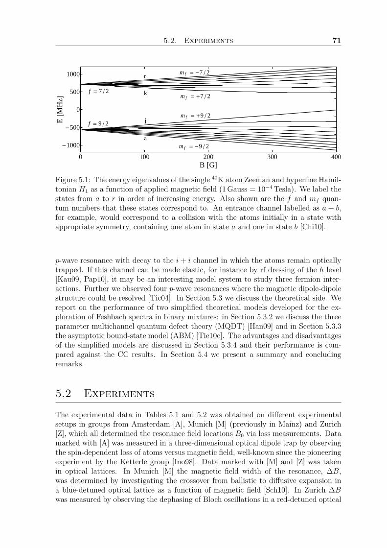
5.2. Experiments 71
f = 7 2
f = 9 2m f = +9 2
m f = -9 2
m f = +7 2
m f = -7 2
a
j
k
r
0 100 200 300 400
-1000
-500
0
500
1000
B @GD
E@M
HzD
Figure 5.1: The energy eigenvalues of the single 40K atom Zeeman and hyperfine Hamil-tonian H1 as a function of applied magnetic field (1Gauss = 10−4 Tesla). We label thestates from a to r in order of increasing energy. Also shown are the f and mf quan-tum numbers that these states correspond to. An entrance channel labelled as a + b,for example, would correspond to a collision with the atoms initially in a state withappropriate symmetry, containing one atom in state a and one in state b [Chi10].
p-wave resonance with decay to the i+ i channel in which the atoms remain opticallytrapped. If this channel can be made elastic, for instance by rf dressing of the h level[Kau09, Pap10], it may be an interesting model system to study three fermion inter-actions. Further we observed four p-wave resonances where the magnetic dipole-dipolestructure could be resolved [Tic04]. In Section 5.3 we discuss the theoretical side. Wereport on the performance of two simplified theoretical models developed for the ex-ploration of Feshbach spectra in binary mixtures: in Section 5.3.2 we discuss the threeparameter multichannel quantum defect theory (MQDT) [Han09] and in Section 5.3.3the asymptotic bound-state model (ABM) [Tie10c]. The advantages and disadvantagesof the simplified models are discussed in Section 5.3.4 and their performance is com-pared against the CC results. In Section 5.4 we present a summary and concludingremarks.
5.2 Experiments
The experimental data in Tables 5.1 and 5.2 was obtained on different experimentalsetups in groups from Amsterdam [A], Munich [M] (previously in Mainz) and Zurich[Z], which all determined the resonance field locations B0 via loss measurements. Datamarked with [A] was measured in a three-dimensional optical dipole trap by observingthe spin-dependent loss of atoms versus magnetic field, well-known since the pioneeringexperiment by the Ketterle group [Ino98]. Data marked with [M] and [Z] was takenin optical lattices. In Munich [M] the magnetic field width of the resonance, ∆B,was determined by investigating the crossover from ballistic to diffusive expansion ina blue-detuned optical lattice as a function of magnetic field [Sch10]. In Zurich ∆Bwas measured by observing the dephasing of Bloch oscillations in a red-detuned optical
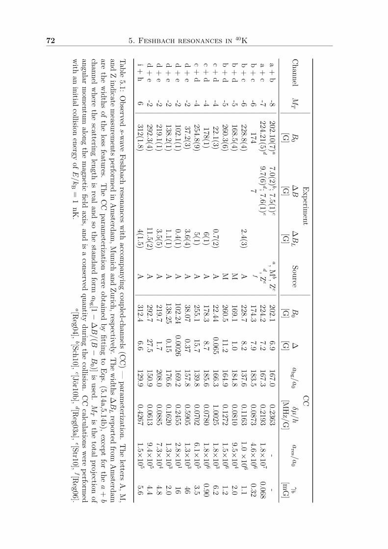
72 5. Feshbach resonances in 40K
Experiment
CC
Channel
MT
B0
∆B
∆BL
SourceB
0∆
abg /a
0δµ/h
ares /a
0γb
[G]
[G]
[G]
[G]
[G]
[MHz/G
][m
G]
a+
b-8
202.10(7)a
7.0(2)b;7.5(1)
ca,M
b,Zc
202.16.9
167.00.2363
--
a+
c-7
224.21(5)d
9.7(6)d;7.6(1)
ed,Z
e224.2
7.2167.3
0.21931.8×
107
0.068b+
c-6
1747
f174.3
7.9183.5
0.08734.6×
106
0.32b+
c-6
228.8(4)2.4(3)
A228.7
8.2137.6
0.11631.0×
106
1.1b+
d-5
168.5(4)M
169.11.0
184.80.0810
9.5×10
42.0
b+
d-5
260.3(6)M
260.511.2
164.90.1272
1.5×10
61.2
c+
d-4
22.1(3)0.7(2)
A22.44
0.065166.3
1.00251.8×
103
6.2c+
d-4
178(1)6(1)
A178.3
8.7185.6
0.07801.8×
106
0.90c+
d-4
254.8(9)5(1)
A255.1
15.7139.8
0.07026.1×
105
3.5d+
e-2
37.2(3)3.6(4)
A38.07
0.37157.8
0.59051.3×
103
46d+
e-2
102.1(1)0.4(1)
A102.24
0.0026169.2
0.24552.8×
101
16d+
e-2
138.2(1)1.1(1)
A138.25
0.15176.6
0.16201.3×
103
2.0d+
e-2
219.1(1)3.5(5)
A219.7
1.7208.0
0.08857.3×
104
4.8d+
e-2
292.3(4)11.5(2)
A292.7
27.5150.9
0.06139.4×
105
4.4i+
h6
312(1.8)4(1.5)
A312.4
6.6129.9
0.42671.5×
105
5.6
Table5.1:
Observed
s-waveFeshbach
resonanceswith
accompanying
coupled-channels(C
C)—
parameterization.
The
lettersA,M
,and
Zindicate
measurem
entsperformed
inAmsterdam
,Munich
andZurich,respectively.T
hewidths∆
BLreported
fromAmsterdam
arethe
widths
ofthe
lossfeatures.
The
CC
parameterization
wereobtained
byfitting
toEqs.(5.14a,5.14b),except
forthe
a+b
channelwhere
thescattering
lengthis
realandso
thestandard
forma
bg [1−
∆B/(B−B
0 )]isused.
MTis
thetotalprojection
ofangular
mom
entumalong
themagnetic
fieldaxis,and
isaconserved
quantityduring
thecollision.
CC
calculationswere
performed
with
aninitialcollision
energyofE/k
B=
1nK
.a[R
eg04],b[Sch10],
c[Jör10b],d[R
eg03a],e[Str10],
f[Reg06].

5.2. Experiments 73
101.5 102.0 102.5 103.0 103.505
1015202530
nu
mber
of at
oms (
x 10
3 )
B (G)Figure 5.2: Determination of the field width of a loss feature around a s-wave resonancein 40K. It is an expanded view of Fig. 5.4. The atom number in the two spin states(squares and triangles) is fitted with a Lorentz distribution (solid line). The center ofthe loss feature we take as B0, the width as ∆BL.
lattice, as was previously demonstrated for the bosonic case in Innsbruck [Gus08].
5.2.1 Experiments in AmsterdamIn Amsterdam the positions of the Feshbach resonances were determined as an increasein the atomic loss rate [Ino98]. To distinguish between losses in the different spin chan-nels all measurements are done with state selective detection. We load about 106 atomsfrom a magnetic trap into a single pass optical dipole trap, created by focusing 1.9Wfrom a fiber laser (λ = 1.07 µm) to a 19 µm waist acting as optical tweezers [Tie10b].The transferred cloud consists of a mixture of atoms in the magnetically trappable spinstates g, h, i, j in the notation of Fig. 5.1. Using the tweezers the cloud is moved intothe center of a Feshbach coil producing the magnetic field for the measurements. Asthe cloud consists of fermions in different spin states it can be evaporatively cooled byreducing the intensity of the trapping light. The spin composition of the mixture isdetermined using the Stern-Gerlach method with typically 104 atoms at the final tem-perature of about 1 µK. We use for this purpose a magnetic field gradient of 100G/cm,applied during the expansion after release from the optical trap. The gradient sepa-rates the different spin states, which are then detected at zero field using absorptionimaging.
In view of the many states of the f = 9/2 ground state hyperfine manifold hundredsof Feshbach resonances can be observed. Therefore, to ensure a proper assignment ofthe Feshbach resonances, it is essential to prepare high purity binary mixtures of onlythe desired spin states. The spin state preparation is done in two steps: firstly, all atomsexcept those in the most populated state j are removed from the sample by a two photoncleaning process at an offset field of 7G. With microwave sweeps the impurity states are
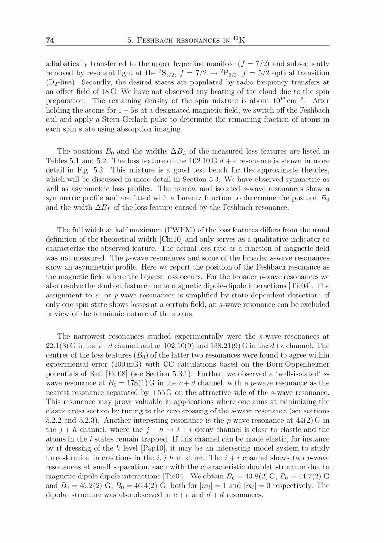
74 5. Feshbach resonances in 40K
adiabatically transferred to the upper hyperfine manifold (f = 7/2) and subsequentlyremoved by resonant light at the 2S1/2, f = 7/2 → 2P3/2, f = 5/2 optical transition(D2-line). Secondly, the desired states are populated by radio frequency transfers atan offset field of 18G. We have not observed any heating of the cloud due to the spinpreparation. The remaining density of the spin mixture is about 1012 cm−3. Afterholding the atoms for 1−5 s at a designated magnetic field, we switch off the Feshbachcoil and apply a Stern-Gerlach pulse to determine the remaining fraction of atoms ineach spin state using absorption imaging.
The positions B0 and the widths ∆BL of the measured loss features are listed inTables 5.1 and 5.2. The loss feature of the 102.10G d+ e resonance is shown in moredetail in Fig. 5.2. This mixture is a good test bench for the approximate theories,which will be discussed in more detail in Section 5.3. We have observed symmetric aswell as asymmetric loss profiles. The narrow and isolated s-wave resonances show asymmetric profile and are fitted with a Lorentz function to determine the position B0and the width ∆BL of the loss feature caused by the Feshbach resonance.
The full width at half maximum (FWHM) of the loss features differs from the usualdefinition of the theoretical width [Chi10] and only serves as a qualitative indicator tocharacterize the observed feature. The actual loss rate as a function of magnetic fieldwas not measured. The p-wave resonances and some of the broader s-wave resonancesshow an asymmetric profile. Here we report the position of the Feshbach resonance asthe magnetic field where the biggest loss occurs. For the broader p-wave resonances wealso resolve the doublet feature due to magnetic dipole-dipole interactions [Tic04]. Theassignment to s- or p-wave resonances is simplified by state dependent detection: ifonly one spin state shows losses at a certain field, an s-wave resonance can be excludedin view of the fermionic nature of the atoms.
The narrowest resonances studied experimentally were the s-wave resonances at22.1(3)G in the c+d channel and at 102.10(9) and 138.21(9)G in the d+e channel. Thecentres of the loss features (B0) of the latter two resonances were found to agree withinexperimental error (100mG) with CC calculations based on the Born-Oppenheimerpotentials of Ref. [Fal08] (see Section 5.3.1). Further, we observed a ‘well-isolated’ s-wave resonance at B0 = 178(1)G in the c+ d channel, with a p-wave resonance as thenearest resonance separated by +55G on the attractive side of the s-wave resonance.This resonance may prove valuable in applications where one aims at minimizing theelastic cross section by tuning to the zero crossing of the s-wave resonance (see sections5.2.2 and 5.2.3). Another interesting resonance is the p-wave resonance at 44(2)G inthe j + h channel, where the j + h → i + i decay channel is close to elastic and theatoms in the i states remain trapped. If this channel can be made elastic, for instanceby rf dressing of the h level [Pap10], it may be an interesting model system to studythree-fermion interactions in the i, j, h mixture. The i + i channel shows two p-waveresonances at small separation, each with the characteristic doublet structure due tomagnetic dipole-dipole interactions [Tic04]. We obtain B0 = 43.8(2)G, B0 = 44.7(2) Gand B0 = 45.2(2) G, B0 = 46.4(2) G, both for |ml| = 1 and |ml| = 0 respectively. Thedipolar structure was also observed in c+ c and d+ d resonances.
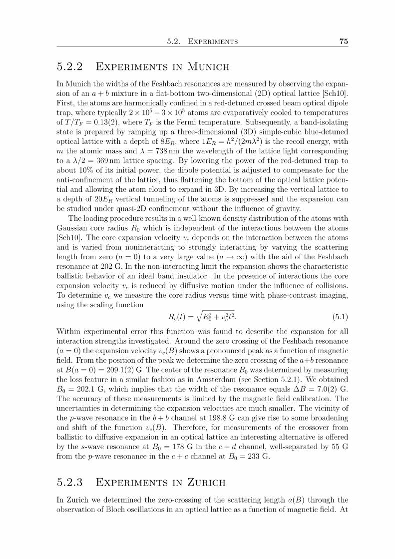
5.2. Experiments 75
5.2.2 Experiments in MunichIn Munich the widths of the Feshbach resonances are measured by observing the expan-sion of an a+ b mixture in a flat-bottom two-dimensional (2D) optical lattice [Sch10].First, the atoms are harmonically confined in a red-detuned crossed beam optical dipoletrap, where typically 2× 10⁵− 3× 10⁵ atoms are evaporatively cooled to temperaturesof T/TF = 0.13(2), where TF is the Fermi temperature. Subsequently, a band-isolatingstate is prepared by ramping up a three-dimensional (3D) simple-cubic blue-detunedoptical lattice with a depth of 8ER, where 1ER = h2/(2mλ2) is the recoil energy, withm the atomic mass and λ = 738nm the wavelength of the lattice light correspondingto a λ/2 = 369 nm lattice spacing. By lowering the power of the red-detuned trap toabout 10% of its initial power, the dipole potential is adjusted to compensate for theanti-confinement of the lattice, thus flattening the bottom of the optical lattice poten-tial and allowing the atom cloud to expand in 3D. By increasing the vertical lattice toa depth of 20ER vertical tunneling of the atoms is suppressed and the expansion canbe studied under quasi-2D confinement without the influence of gravity.
The loading procedure results in a well-known density distribution of the atoms withGaussian core radius R0 which is independent of the interactions between the atoms[Sch10]. The core expansion velocity vc depends on the interaction between the atomsand is varied from noninteracting to strongly interacting by varying the scatteringlength from zero (a = 0) to a very large value (a → ∞) with the aid of the Feshbachresonance at 202 G. In the non-interacting limit the expansion shows the characteristicballistic behavior of an ideal band insulator. In the presence of interactions the coreexpansion velocity vc is reduced by diffusive motion under the influence of collisions.To determine vc we measure the core radius versus time with phase-contrast imaging,using the scaling function
Rc(t) =√R2
0 + v2c t
2. (5.1)
Within experimental error this function was found to describe the expansion for allinteraction strengths investigated. Around the zero crossing of the Feshbach resonance(a = 0) the expansion velocity vc(B) shows a pronounced peak as a function of magneticfield. From the position of the peak we determine the zero crossing of the a+b resonanceat B(a = 0) = 209.1(2) G. The center of the resonance B0 was determined by measuringthe loss feature in a similar fashion as in Amsterdam (see Section 5.2.1). We obtainedB0 = 202.1 G, which implies that the width of the resonance equals ∆B = 7.0(2) G.The accuracy of these measurements is limited by the magnetic field calibration. Theuncertainties in determining the expansion velocities are much smaller. The vicinity ofthe p-wave resonance in the b+ b channel at 198.8 G can give rise to some broadeningand shift of the function vc(B). Therefore, for measurements of the crossover fromballistic to diffusive expansion in an optical lattice an interesting alternative is offeredby the s-wave resonance at B0 = 178 G in the c + d channel, well-separated by 55 Gfrom the p-wave resonance in the c+ c channel at B0 = 233 G.
5.2.3 Experiments in ZurichIn Zurich we determined the zero-crossing of the scattering length a(B) through theobservation of Bloch oscillations in an optical lattice as a function of magnetic field. At
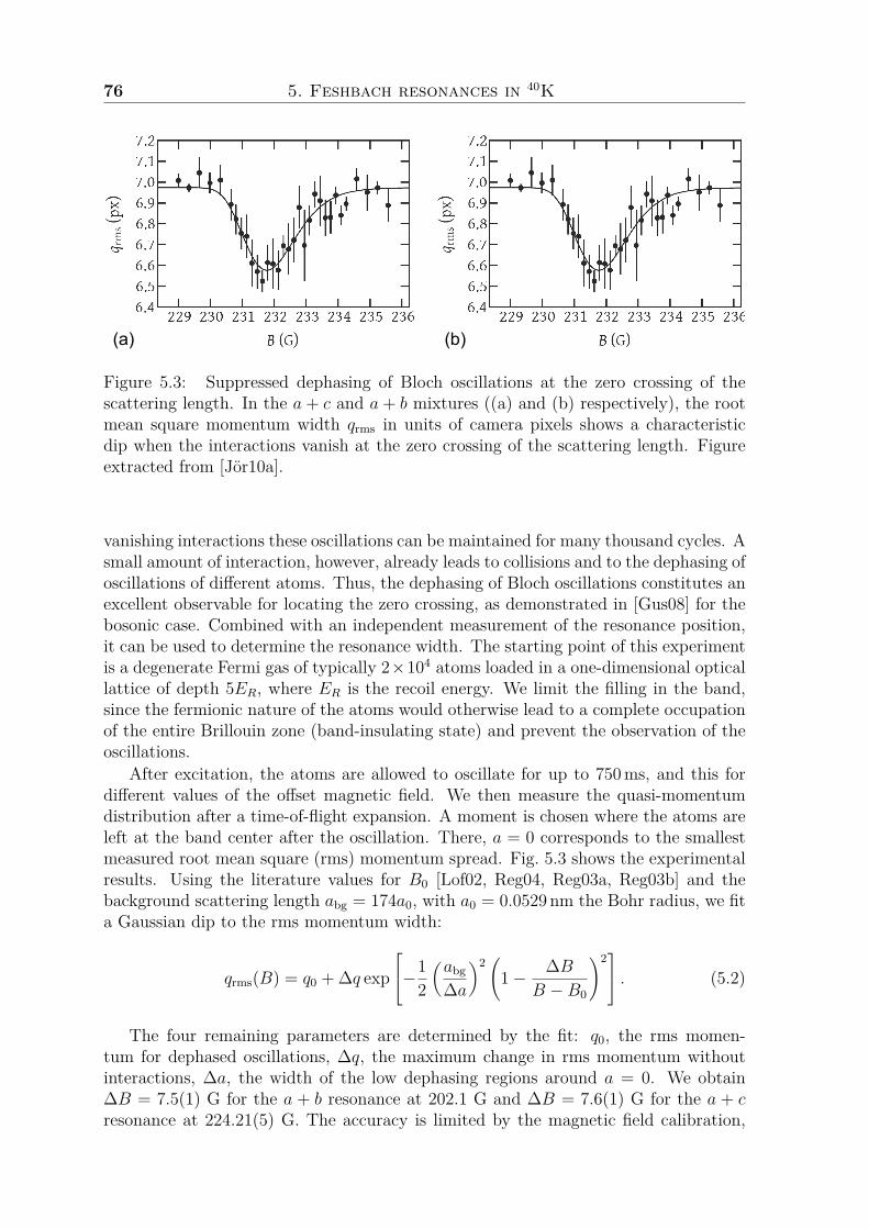
76 5. Feshbach resonances in 40K
(a) (b)
Figure 5.3: Suppressed dephasing of Bloch oscillations at the zero crossing of thescattering length. In the a+ c and a+ b mixtures ((a) and (b) respectively), the rootmean square momentum width qrms in units of camera pixels shows a characteristicdip when the interactions vanish at the zero crossing of the scattering length. Figureextracted from [Jör10a].
vanishing interactions these oscillations can be maintained for many thousand cycles. Asmall amount of interaction, however, already leads to collisions and to the dephasing ofoscillations of different atoms. Thus, the dephasing of Bloch oscillations constitutes anexcellent observable for locating the zero crossing, as demonstrated in [Gus08] for thebosonic case. Combined with an independent measurement of the resonance position,it can be used to determine the resonance width. The starting point of this experimentis a degenerate Fermi gas of typically 2×10⁴ atoms loaded in a one-dimensional opticallattice of depth 5ER, where ER is the recoil energy. We limit the filling in the band,since the fermionic nature of the atoms would otherwise lead to a complete occupationof the entire Brillouin zone (band-insulating state) and prevent the observation of theoscillations.
After excitation, the atoms are allowed to oscillate for up to 750ms, and this fordifferent values of the offset magnetic field. We then measure the quasi-momentumdistribution after a time-of-flight expansion. A moment is chosen where the atoms areleft at the band center after the oscillation. There, a = 0 corresponds to the smallestmeasured root mean square (rms) momentum spread. Fig. 5.3 shows the experimentalresults. Using the literature values for B0 [Lof02, Reg04, Reg03a, Reg03b] and thebackground scattering length abg = 174a0, with a0 = 0.0529nm the Bohr radius, we fita Gaussian dip to the rms momentum width:
qrms(B) = q0 + ∆q exp−1
2
(abg
∆a
)2(
1− ∆BB −B0
)2 . (5.2)
The four remaining parameters are determined by the fit: q0, the rms momen-tum for dephased oscillations, ∆q, the maximum change in rms momentum withoutinteractions, ∆a, the width of the low dephasing regions around a = 0. We obtain∆B = 7.5(1) G for the a + b resonance at 202.1 G and ∆B = 7.6(1) G for the a + cresonance at 224.21(5) G. The accuracy is limited by the magnetic field calibration,

5.2. Experiments 77
the uncertainty of the resonance position and the width of the dip. Compared to ex-perimental values obtained at JILA [Reg03a], the width of the a+ c resonance differs.However, it is consistent with the value of the on-site-interaction U extracted fromlattice modulation spectroscopy in a three-dimensional optical lattice [Jör10b]. Addi-tionally we have observed a previously unreported p-wave Feshbach resonance in thec + c channel which shows the characteristic doublet feature due to magnetic dipole-dipole interactions [Tic04]. We obtain B0 = 232.8(2) G and B0 = 233.4(2) G for|ml| = 1 and |ml| = 0 respectively. Here ml is projection of the orbital angular mo-mentum on the magnetic field axis. The assignment of the loss features to a p-waveresonance is confirmed by the suppression of either the |ml| = 0 or the |ml| = 1 reso-nance when the experiments are realized in a one-dimensional geometry, depending onthe relative orientation of the magnetic field axis and the extension of the gas [Gün05].
Experiment CCChannel MT B0 [G] Source B0 [G]a + c -7 215(5) M 215.0b + b -6, -8 198.30(2) [Gae07] 198.4b + b -7 198.80(5) [Gae07] 198.9c + c -4,-6 232.8(2) [Z]; 232.8(2) [A] Z/A 233.0c + c -5 233.4(2) [Z]; 233.6(2) [A] Z/A 233.6c + c -5 245.3(5) [M]; 245.4(4) [A] M/A 245.0c + d -3,-5 262.2(2) A 262.2c + d -4 262.6(2) A 262.5d + d -3 287(1.8) A 287.6d + d -3 311.8(4) A 311.8d + e -2 338(1.8) A 338.4e + e -1 373(1.8) A 373.7h + h 5 68(1.8) A 67.6h + h 5 102(1.8) A 100.2h + h 5 139(1.8) A 138.0h + h 5 324(1.8) A 323.1h + j 7 44(1.8) A 44.6i + i 6,8 43.8(2) A 43.6i + i 7 44.7(2) A 44.9i + i 6,8 45.2(2) A 45.3i + i 7 46.4(2) A 46.4
Table 5.2: Observed p-wave Feshbach resonances with accompanying coupled-channels(CC) parameterizations. The letters A, M, and Z refer to measurements performed inAmsterdam, Munich and Zurich, respectively. MT is the total projection of angularmomentum along the magnetic field axis, for each collision channel it can take onthree values corresponding to different projections of the orbital angular momentumquantum number ml = 0,±1. CC calculations were performed at an initial collisionenergy of E/kB = 1 µK. This accounts for the discrepancy between the calculatedpositions in the b + b channel with Ref. [Gae07] where effort was made to account forthe temperature dependence.
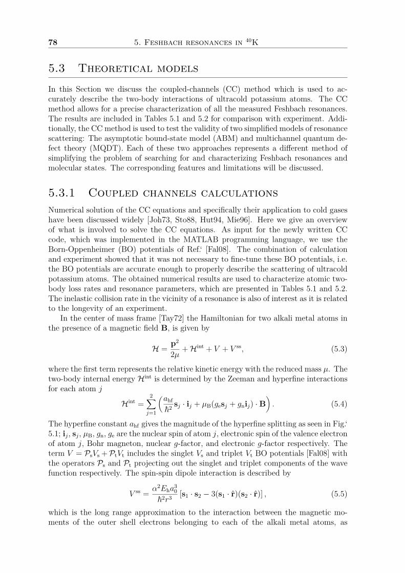
78 5. Feshbach resonances in 40K
5.3 Theoretical modelsIn this Section we discuss the coupled-channels (CC) method which is used to ac-curately describe the two-body interactions of ultracold potassium atoms. The CCmethod allows for a precise characterization of all the measured Feshbach resonances.The results are included in Tables 5.1 and 5.2 for comparison with experiment. Addi-tionally, the CC method is used to test the validity of two simplified models of resonancescattering: The asymptotic bound-state model (ABM) and multichannel quantum de-fect theory (MQDT). Each of these two approaches represents a different method ofsimplifying the problem of searching for and characterizing Feshbach resonances andmolecular states. The corresponding features and limitations will be discussed.
5.3.1 Coupled channels calculationsNumerical solution of the CC equations and specifically their application to cold gaseshave been discussed widely [Joh73, Sto88, Hut94, Mie96]. Here we give an overviewof what is involved to solve the CC equations. As input for the newly written CCcode, which was implemented in the MATLAB programming language, we use theBorn-Oppenheimer (BO) potentials of Ref.‘ [Fal08]. The combination of calculationand experiment showed that it was not necessary to fine-tune these BO potentials, i.e.the BO potentials are accurate enough to properly describe the scattering of ultracoldpotassium atoms. The obtained numerical results are used to characterize atomic two-body loss rates and resonance parameters, which are presented in Tables 5.1 and 5.2.The inelastic collision rate in the vicinity of a resonance is also of interest as it is relatedto the longevity of an experiment.
In the center of mass frame [Tay72] the Hamiltonian for two alkali metal atoms inthe presence of a magnetic field B, is given by
H = p2
2µ +Hint + V + V ss, (5.3)
where the first term represents the relative kinetic energy with the reduced mass µ. Thetwo-body internal energy Hint is determined by the Zeeman and hyperfine interactionsfor each atom j
Hint =2∑j=1
(ahf
~2 sj · ij + µB(gesj + gnij) ·B). (5.4)
The hyperfine constant ahf gives the magnitude of the hyperfine splitting as seen in Fig.‘5.1; ij, sj, µB, gn, ge are the nuclear spin of atom j, electronic spin of the valence electronof atom j, Bohr magneton, nuclear g-factor, and electronic g-factor respectively. Theterm V = PsVs +PtVt includes the singlet Vs and triplet Vt BO potentials [Fal08] withthe operators Ps and Pt projecting out the singlet and triplet components of the wavefunction respectively. The spin-spin dipole interaction is described by
V ss = α2Eha30
~2r3 [s1 · s2 − 3(s1 · r)(s2 · r)] , (5.5)
which is the long range approximation to the interaction between the magnetic mo-ments of the outer shell electrons belonging to each of the alkali metal atoms, as
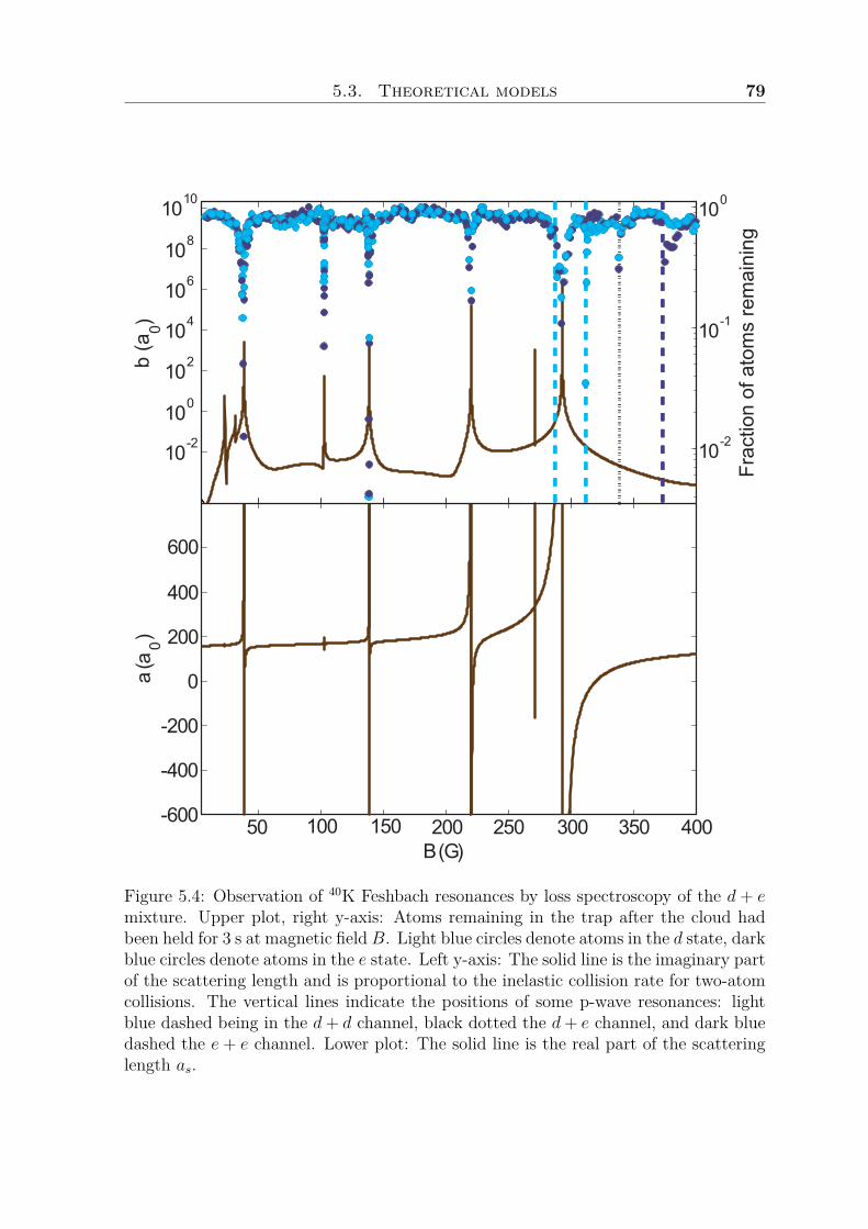
5.3. Theoretical models 79
10-2
100
102
104
106
108
1010
b (a
0)
50 100 150 200 250 300 350 400-600
-400
-200
0
200
400
600
B (G)
a (a
0)
10-2
10-1
100
Frac
tion
of a
tom
s re
mai
ning
Figure 5.4: Observation of 40K Feshbach resonances by loss spectroscopy of the d + emixture. Upper plot, right y-axis: Atoms remaining in the trap after the cloud hadbeen held for 3 s at magnetic field B. Light blue circles denote atoms in the d state, darkblue circles denote atoms in the e state. Left y-axis: The solid line is the imaginary partof the scattering length and is proportional to the inelastic collision rate for two-atomcollisions. The vertical lines indicate the positions of some p-wave resonances: lightblue dashed being in the d+ d channel, black dotted the d+ e channel, and dark bluedashed the e + e channel. Lower plot: The solid line is the real part of the scatteringlength as.

80 5. Feshbach resonances in 40K
discussed in Ref.‘ [Sto88]. Here r, Eh, and α are the interatomic separation, Hartreeenergy, and fine structure constant respectively.
Starting from the rigorous multichannel scattering theory it is possible to derivethe coupled-channels equations in the close-coupling approximation [Tay72, New66].Hereby we express the wave function in terms of the N (channel) states |σm〉, thatdiagonalize the Hamiltonian Hint and have the correct symmetry,
1r
N∑m=1|σm〉ψm(r). (5.6)
The radial Schrödinger equation can now be projected on the channel states whichyields N equations
∂2ψm∂r2 = 2µ
~2
N∑n=1
[Wm,n(r) + V ss
m,n − Eδm,n]ψn(r) (5.7)
where δm,n is the Kronecker delta and
Wm,n(r) = δm,n
[En + ~2
2µln(ln + 1)
r2
]+ Vm,n. (5.8)
Here En is the eigen-energy of the internal Hamiltonian Hint and ln is the relativeorbital angular momentum quantum number of the state |σn〉. It is useful to rewritethis set of equations in the N ×N matrix form
Ψ′′(r) = [Q(r) + Vss(r)] Ψ(r), (5.9)
where the elements of the matrix Q(r) are given by (2µ/~2)[Wm,n(r)−Eδm,n]. Consid-ering the scattering boundary condition (i.e. r → ∞), [Ψ]1,...,N,m can be interpretedas being the scattering wave function with an incoming wave in channel m. In prac-tice, rather than propagating the wave function and derivative matrices to large r,we instead propagate the log-derivative matrix Y = Ψ′[Ψ]−1 using the technique ofManolopoulos [Man86]. With this in mind a multichannel S matrix can be extractedvia [Tay72]
S(r) =[Y(r)h(1)(r)− h′(1)(r)
]−1×[h′(2)(r)−Y(r)h(2)(r)
], (5.10)
where [h(1,2)(r)]m,n = −δm,n√knirh
(1,2)ln
are diagonal matrices with h(1)ln
and h(2)ln
rep-resenting spherical Hankel functions of the first and second kind. The asymptoticmagnitude of the momentum in channel |σn〉 equals ~kn =
√2µ(E − En). For non-
s-wave entrance channels the numerical propagation becomes difficult at low collisionenergies. We find it necessary to use the long range approximate correction to the Smatrix given by [Sto88]
S(∞) ≈ S(r1)− i µ~2
∫ ∞r1
[h(2)(r) + S(r1)h(1)(r)
]× Vss(r)
[h(2)(r) + h(1)(r)S(r1)
]dr
(5.11)in order to greatly increase the rate of convergence. This expression assumes that r1is large enough to neglect contributions from V , which fall off as r−6. The integration
5.3. Theoretical models 81
in this expression is performed analytically. We only include open channels in thiscorrection.
Although we have thus far formulated the problem using |σi〉, it is also useful toemploy an alternative set of angular momentum states. In the inner region, wherethe singlet and triplet potentials are dominant, we use a basis in which i1 and i2 arecoupled to give I, and s1 and s2 are coupled to give S. This has the advantage of theBO contribution V being diagonal. We perform the basis transformation to the basisstates |σm〉 at the internuclear distance where the energy difference |Vt − Vs| is largecompared to the atomic hyperfine coupling.
Once an S matrix has been evaluated one can extract the s-wave scattering lengthby defining the phase shift δ(E), related to the element of the S matrix [S]e,e =exp[2iδ(E)], with e indicating the entrance channel. If the entrance channel is theonly open channel the scattering length is given by the limiting process
a = limk→0
− tan[δ(E)]k
. (5.12)
This can be generalized to the case where the scattering is not purely elastic; i.e., thereis more than one open channel. Here the complex scattering length a and complexphase shift δ(E) are now related by
a = a− bi = limk→0
− tan[δ(E)]k
. (5.13)
It can be shown, see Refs. [Nai11, Hut07, Boh99, Fed96], that in the vicinity of aFeshbach resonance the following parameterization is valid
a(B) = abg
(1− ∆B(B −B0)
(B −B0)2 + (γB/2)2
), (5.14a)
b(B) = 2ares(γB/2)2
(B −B0)2 + (γB/2)2 . (5.14b)
In these expressions, abg is the background scattering length, representing the scatteringlength of the entrance channel in the absence of a resonance. We have expressedthe decay rate of the bound state, γ [Köh05], in magnetic field units, γB = ~γ/µres,where µres is the difference in magnetic moment between the entrance channel andthe bound state causing the resonance. The resonance length ares is defined by ares =abg∆B/γB and characterizes the strength of a resonance. The width and the centerof the resonance are given by ∆B and B0, respectively. The real part of the complexscattering length a is still the appropriate parameter to describe the elastic scatteringprocess, while the imaginary part can be used to describe the inelastic collision ratecoefficient for channels with two atoms in different spin states
K2(B) = 4π~µb(B). (5.15)
In the limit of zero collisional energy this rate has its peak exactly on resonance whereit equals K2(B0) = 8π~ares/µ. In a thermal gas at kBT γB the rate drops rapidlywith temperature, K2(B0) ∝ T−2. For partial densities nα and nβ the total decayrate of component α is given by −nα/nα = K2nβ + τ−1
vac, where τvac is the vacuum
82 5. Feshbach resonances in 40K
0 50 100 150 200 250 300-25
-20
-15
-10
-5
0
B (G)
E/h
(MH
z)
250 275 300
-2
-1
0
Figure 5.5: (Color online) Energy spectrum of s-wave molecular levels of 40K in thed+ e channel. Energies are given relative to the d+ e threshold. The binding energieswere obtained using: the CC method (black line), the MQDT (red dashed line), andthe ABM (green dot-dashed line). The inset shows the binding energies near the broadresonance around B ' 290 G. For the MQDT and ABM the optimized parameterswere used as input. The results for ABM are shown without the dressing of the boundstate [Tie10c], except in the inset (green dotted line).
lifetime. Some results of the CC calculation for the real and imaginary parts a(B)and b(B) of the scattering length are shown for the d + e mixture in Fig.‘ 5.4, wherethey can be compared to experimental findings. For all observed s-wave resonancesthe calculated values for B0, ∆B, abg, ares, γB and µres were obtained for a collisionenergy E/kB = 1 µK and are tabulated in Table 5.1. For the p-wave resonances thecollision energy was E/kB = 1 µK and only the position B0 of the resonance center istabulated.
The bound state calculations are performed as in Ref. [Hut94]. They involve nu-merical methods similar to those used for the scattering calculations. However theasymptotic r → ∞ boundary condition on Ψ(r) now requires that all elements decaysuitably to zero. The term Vss(r) is neglected in the bound state calculations becausethey are used for comparison to the MQDT and the ABM (see Fig.‘ 5.5), neither ofwhich include this term. We propagate Y(r) from small r outwards to some matchingpoint R, which we call Ya. We then propagate from large r inwards to R which wecall Yb. It can be shown that a bound state exists if the matching matrix
M(E) = Ya −Yb (5.16)
has an eigenvalue equal to zero.
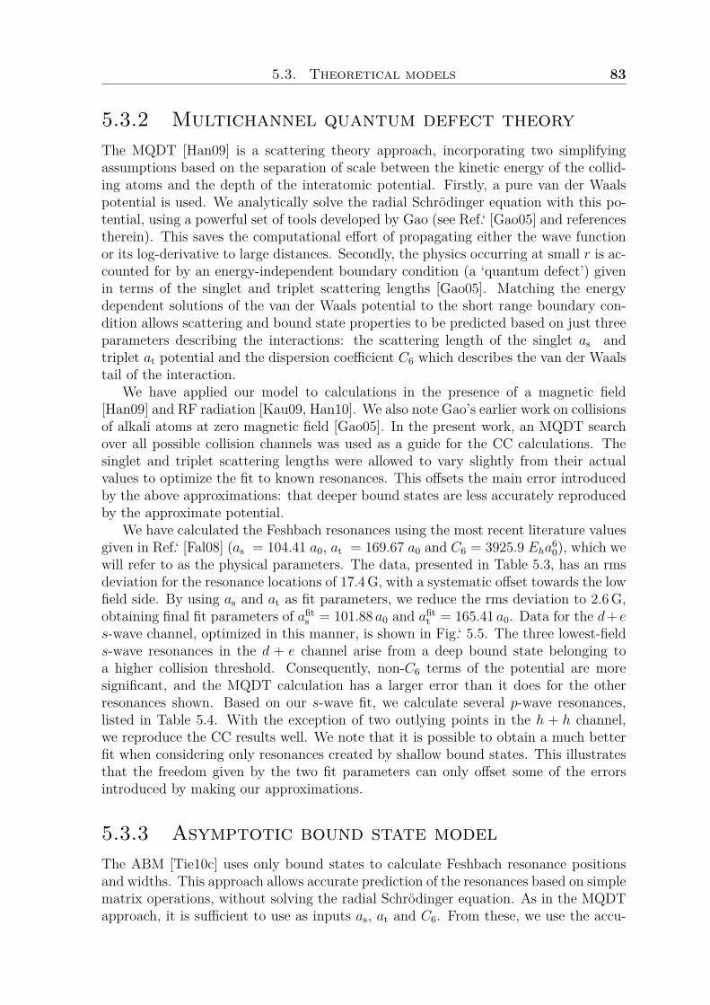
5.3. Theoretical models 83
5.3.2 Multichannel quantum defect theoryThe MQDT [Han09] is a scattering theory approach, incorporating two simplifyingassumptions based on the separation of scale between the kinetic energy of the collid-ing atoms and the depth of the interatomic potential. Firstly, a pure van der Waalspotential is used. We analytically solve the radial Schrödinger equation with this po-tential, using a powerful set of tools developed by Gao (see Ref.‘ [Gao05] and referencestherein). This saves the computational effort of propagating either the wave functionor its log-derivative to large distances. Secondly, the physics occurring at small r is ac-counted for by an energy-independent boundary condition (a ‘quantum defect’) givenin terms of the singlet and triplet scattering lengths [Gao05]. Matching the energydependent solutions of the van der Waals potential to the short range boundary con-dition allows scattering and bound state properties to be predicted based on just threeparameters describing the interactions: the scattering length of the singlet as andtriplet at potential and the dispersion coefficient C6 which describes the van der Waalstail of the interaction.
We have applied our model to calculations in the presence of a magnetic field[Han09] and RF radiation [Kau09, Han10]. We also note Gao’s earlier work on collisionsof alkali atoms at zero magnetic field [Gao05]. In the present work, an MQDT searchover all possible collision channels was used as a guide for the CC calculations. Thesinglet and triplet scattering lengths were allowed to vary slightly from their actualvalues to optimize the fit to known resonances. This offsets the main error introducedby the above approximations: that deeper bound states are less accurately reproducedby the approximate potential.
We have calculated the Feshbach resonances using the most recent literature valuesgiven in Ref.‘ [Fal08] (as = 104.41 a0, at = 169.67 a0 and C6 = 3925.9 Eha6
0), which wewill refer to as the physical parameters. The data, presented in Table 5.3, has an rmsdeviation for the resonance locations of 17.4G, with a systematic offset towards the lowfield side. By using as and at as fit parameters, we reduce the rms deviation to 2.6G,obtaining final fit parameters of afits = 101.88 a0 and afitt = 165.41 a0. Data for the d+ es-wave channel, optimized in this manner, is shown in Fig.‘ 5.5. The three lowest-fields-wave resonances in the d + e channel arise from a deep bound state belonging toa higher collision threshold. Consequently, non-C6 terms of the potential are moresignificant, and the MQDT calculation has a larger error than it does for the otherresonances shown. Based on our s-wave fit, we calculate several p-wave resonances,listed in Table 5.4. With the exception of two outlying points in the h + h channel,we reproduce the CC results well. We note that it is possible to obtain a much betterfit when considering only resonances created by shallow bound states. This illustratesthat the freedom given by the two fit parameters can only offset some of the errorsintroduced by making our approximations.
5.3.3 Asymptotic bound state modelThe ABM [Tie10c] uses only bound states to calculate Feshbach resonance positionsand widths. This approach allows accurate prediction of the resonances based on simplematrix operations, without solving the radial Schrödinger equation. As in the MQDTapproach, it is sufficient to use as inputs as, at and C6. From these, we use the accu-
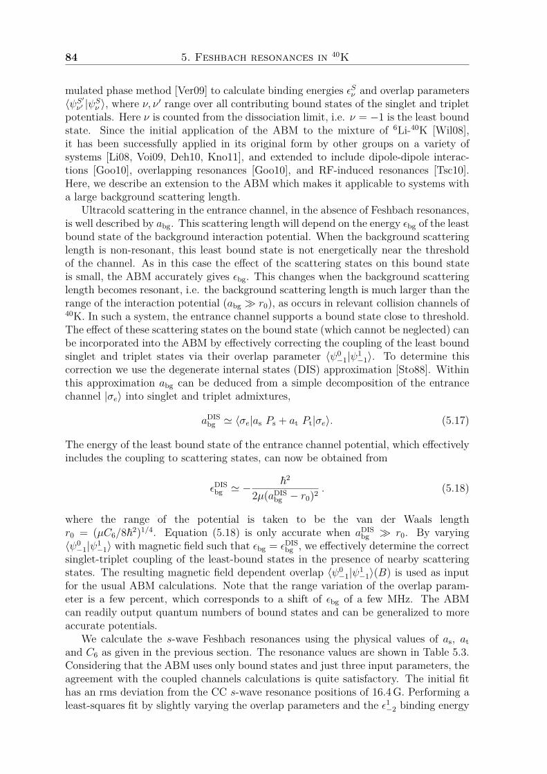
84 5. Feshbach resonances in 40K
mulated phase method [Ver09] to calculate binding energies εSν and overlap parameters〈ψS′ν′ |ψSν 〉, where ν, ν ′ range over all contributing bound states of the singlet and tripletpotentials. Here ν is counted from the dissociation limit, i.e. ν = −1 is the least boundstate. Since the initial application of the ABM to the mixture of 6Li-40K [Wil08],it has been successfully applied in its original form by other groups on a variety ofsystems [Li08, Voi09, Deh10, Kno11], and extended to include dipole-dipole interac-tions [Goo10], overlapping resonances [Goo10], and RF-induced resonances [Tsc10].Here, we describe an extension to the ABM which makes it applicable to systems witha large background scattering length.
Ultracold scattering in the entrance channel, in the absence of Feshbach resonances,is well described by abg. This scattering length will depend on the energy εbg of the leastbound state of the background interaction potential. When the background scatteringlength is non-resonant, this least bound state is not energetically near the thresholdof the channel. As in this case the effect of the scattering states on this bound stateis small, the ABM accurately gives εbg. This changes when the background scatteringlength becomes resonant, i.e. the background scattering length is much larger than therange of the interaction potential (abg r0), as occurs in relevant collision channels of40K. In such a system, the entrance channel supports a bound state close to threshold.The effect of these scattering states on the bound state (which cannot be neglected) canbe incorporated into the ABM by effectively correcting the coupling of the least boundsinglet and triplet states via their overlap parameter 〈ψ0
−1|ψ1−1〉. To determine this
correction we use the degenerate internal states (DIS) approximation [Sto88]. Withinthis approximation abg can be deduced from a simple decomposition of the entrancechannel |σe〉 into singlet and triplet admixtures,
aDISbg ' 〈σe|as Ps + at Pt|σe〉. (5.17)
The energy of the least bound state of the entrance channel potential, which effectivelyincludes the coupling to scattering states, can now be obtained from
εDISbg ' −
~2
2µ(aDISbg − r0)2 . (5.18)
where the range of the potential is taken to be the van der Waals lengthr0 = (µC6/8~2)1/4. Equation (5.18) is only accurate when aDIS
bg r0. By varying〈ψ0−1|ψ1
−1〉 with magnetic field such that εbg = εDISbg , we effectively determine the correct
singlet-triplet coupling of the least-bound states in the presence of nearby scatteringstates. The resulting magnetic field dependent overlap 〈ψ0
−1|ψ1−1〉(B) is used as input
for the usual ABM calculations. Note that the range variation of the overlap param-eter is a few percent, which corresponds to a shift of εbg of a few MHz. The ABMcan readily output quantum numbers of bound states and can be generalized to moreaccurate potentials.
We calculate the s-wave Feshbach resonances using the physical values of as, atand C6 as given in the previous section. The resonance values are shown in Table 5.3.Considering that the ABM uses only bound states and just three input parameters, theagreement with the coupled channels calculations is quite satisfactory. The initial fithas an rms deviation from the CC s-wave resonance positions of 16.4G. Performing aleast-squares fit by slightly varying the overlap parameters and the ε1−2 binding energy
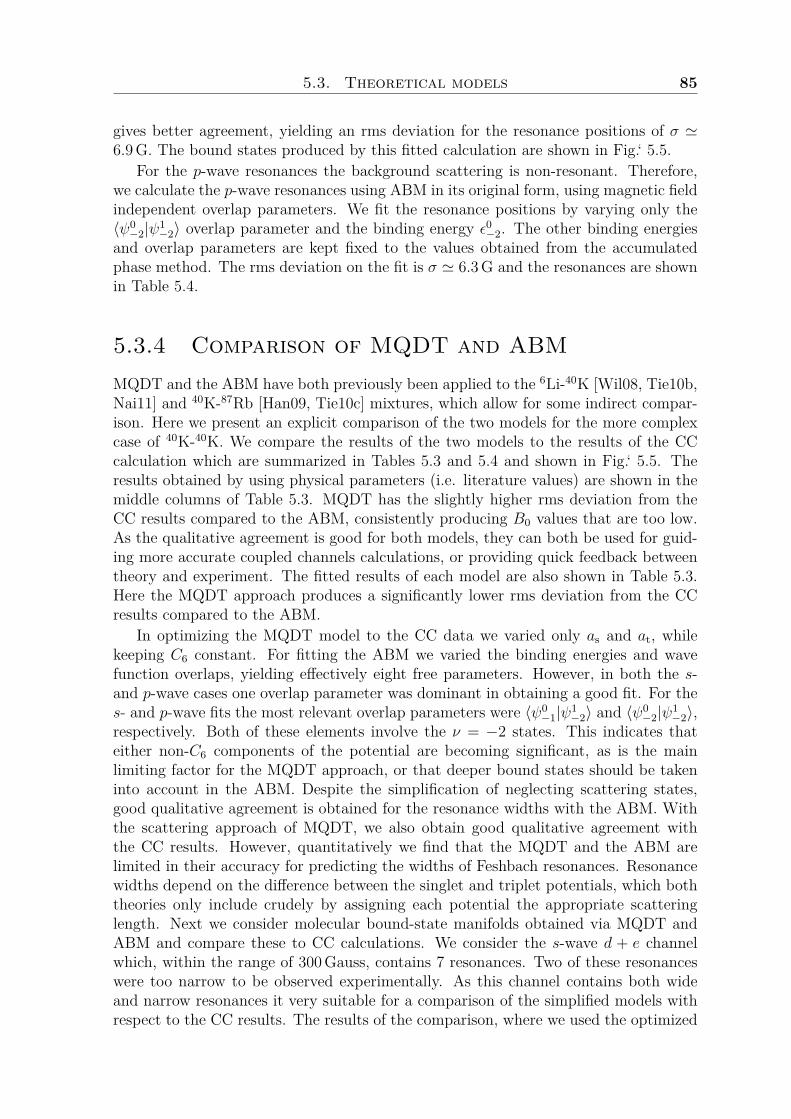
5.3. Theoretical models 85
gives better agreement, yielding an rms deviation for the resonance positions of σ '6.9G. The bound states produced by this fitted calculation are shown in Fig.‘ 5.5.
For the p-wave resonances the background scattering is non-resonant. Therefore,we calculate the p-wave resonances using ABM in its original form, using magnetic fieldindependent overlap parameters. We fit the resonance positions by varying only the〈ψ0−2|ψ1
−2〉 overlap parameter and the binding energy ε0−2. The other binding energiesand overlap parameters are kept fixed to the values obtained from the accumulatedphase method. The rms deviation on the fit is σ ' 6.3G and the resonances are shownin Table 5.4.
5.3.4 Comparison of MQDT and ABMMQDT and the ABM have both previously been applied to the 6Li-40K [Wil08, Tie10b,Nai11] and 40K-87Rb [Han09, Tie10c] mixtures, which allow for some indirect compar-ison. Here we present an explicit comparison of the two models for the more complexcase of 40K-40K. We compare the results of the two models to the results of the CCcalculation which are summarized in Tables 5.3 and 5.4 and shown in Fig.‘ 5.5. Theresults obtained by using physical parameters (i.e. literature values) are shown in themiddle columns of Table 5.3. MQDT has the slightly higher rms deviation from theCC results compared to the ABM, consistently producing B0 values that are too low.As the qualitative agreement is good for both models, they can both be used for guid-ing more accurate coupled channels calculations, or providing quick feedback betweentheory and experiment. The fitted results of each model are also shown in Table 5.3.Here the MQDT approach produces a significantly lower rms deviation from the CCresults compared to the ABM.
In optimizing the MQDT model to the CC data we varied only as and at, whilekeeping C6 constant. For fitting the ABM we varied the binding energies and wavefunction overlaps, yielding effectively eight free parameters. However, in both the s-and p-wave cases one overlap parameter was dominant in obtaining a good fit. For thes- and p-wave fits the most relevant overlap parameters were 〈ψ0
−1|ψ1−2〉 and 〈ψ0
−2|ψ1−2〉,
respectively. Both of these elements involve the ν = −2 states. This indicates thateither non-C6 components of the potential are becoming significant, as is the mainlimiting factor for the MQDT approach, or that deeper bound states should be takeninto account in the ABM. Despite the simplification of neglecting scattering states,good qualitative agreement is obtained for the resonance widths with the ABM. Withthe scattering approach of MQDT, we also obtain good qualitative agreement withthe CC results. However, quantitatively we find that the MQDT and the ABM arelimited in their accuracy for predicting the widths of Feshbach resonances. Resonancewidths depend on the difference between the singlet and triplet potentials, which boththeories only include crudely by assigning each potential the appropriate scatteringlength. Next we consider molecular bound-state manifolds obtained via MQDT andABM and compare these to CC calculations. We consider the s-wave d + e channelwhich, within the range of 300Gauss, contains 7 resonances. Two of these resonanceswere too narrow to be observed experimentally. As this channel contains both wideand narrow resonances it very suitable for a comparison of the simplified models withrespect to the CC results. The results of the comparison, where we used the optimized
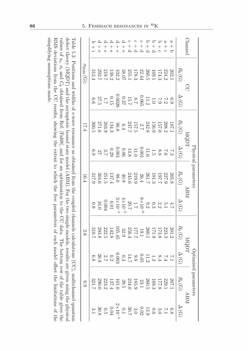
86 5. Feshbach resonances in 40K
Physicalparameters
Optim
isedparam
etersChannel
CC
MQDT
ABM
MQDT
ABM
B0 (G
)∆
(G)
B0 (G
)∆(G
)B
0 (G)
∆(G
)B
0 (G)
∆(G
)B
0 (G)
∆(G
)a+
b202.1
6.9187.1
7.3205.8
4.7201.2
7.1207.1
6.8a+
c224.2
7.2208.2
7.6227.9
5.1223.3
7.4229.1
7.1b+
c174.3
7.9157.0
8.8197.7
2.2173.8
8.4177.8
3.0b+
d169.1
1.0156.9
1.5181.3
0.3171.9
1.3169.3
0.6b+
d260.5
11.2242.8
11.6261.7
9.2260.1
11.2260.5
13.9c+
d22.44
0.0652.7
0.00126.4
8×10−
619.1
0.0523.1
0.02c+
d178.3
8.7157.5
11.0219.9
1.7177.7
9.8185.9
3.0c+
d255.1
15.7237.7
14.8245.6
20.7256.4
14.7234.0
30.7d+
e38.07
0.376.4
0.0640.9
4×10−
532.9
0.339.5
0.1d+
e102.2
0.002698.8
0.00198.0
3×10−
4105.45
0.003101.0
2×10−
4
d+
e138.2
0.15134.3
0.29137.4
0.01142.8
0.2137.4
0.04d+
e219.7
1.7203.9
3.7251.5
0.004222.5
2.7223.2
0.5d+
e292.7
27.5271.6
27304.6
16.0293.8
26.8290.0
30.8h+
i312.4
6.6300.5
6.9317.9
0.9310.7
6.8321.7
3.1σRMS (G
):17.4
16.42.6
6.9
Table5.3:Positionsand
widthsof
s-waveresonance
asobtainedfrom
thecoupled
channelscalculations(CC),m
ultichannelquantumdefecttheory
(MQDT)and
theasym
ptoticbound
statemodel(A
BM).Forthe
twosim
plemodels,resultsare
givenusing
thephysical
valuesofas ,at and
C6obtained
fromRef.[Fal08],and
foran
optimisation
tothe
CC
data.The
bottomrow
ofthetable
givesthe
RMSdeviations
fromthe
CC
results,showing
theextent
towhich
thefree
parameters
ofeach
modeloffset
thelim
itationsof
thesim
plifyingassum
ptionsmade.
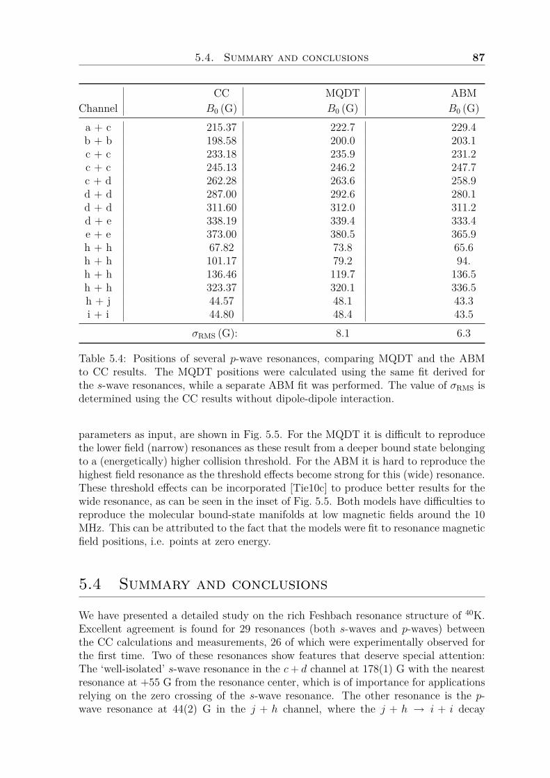
5.4. Summary and conclusions 87
CC MQDT ABMChannel B0 (G) B0 (G) B0 (G)a + c 215.37 222.7 229.4b + b 198.58 200.0 203.1c + c 233.18 235.9 231.2c + c 245.13 246.2 247.7c + d 262.28 263.6 258.9d + d 287.00 292.6 280.1d + d 311.60 312.0 311.2d + e 338.19 339.4 333.4e + e 373.00 380.5 365.9h + h 67.82 73.8 65.6h + h 101.17 79.2 94.h + h 136.46 119.7 136.5h + h 323.37 320.1 336.5h + j 44.57 48.1 43.3i + i 44.80 48.4 43.5
σRMS (G): 8.1 6.3
Table 5.4: Positions of several p-wave resonances, comparing MQDT and the ABMto CC results. The MQDT positions were calculated using the same fit derived forthe s-wave resonances, while a separate ABM fit was performed. The value of σRMS isdetermined using the CC results without dipole-dipole interaction.
parameters as input, are shown in Fig. 5.5. For the MQDT it is difficult to reproducethe lower field (narrow) resonances as these result from a deeper bound state belongingto a (energetically) higher collision threshold. For the ABM it is hard to reproduce thehighest field resonance as the threshold effects become strong for this (wide) resonance.These threshold effects can be incorporated [Tie10c] to produce better results for thewide resonance, as can be seen in the inset of Fig. 5.5. Both models have difficulties toreproduce the molecular bound-state manifolds at low magnetic fields around the 10MHz. This can be attributed to the fact that the models were fit to resonance magneticfield positions, i.e. points at zero energy.
5.4 Summary and conclusions
We have presented a detailed study on the rich Feshbach resonance structure of 40K.Excellent agreement is found for 29 resonances (both s-waves and p-waves) betweenthe CC calculations and measurements, 26 of which were experimentally observed forthe first time. Two of these resonances show features that deserve special attention:The ‘well-isolated’ s-wave resonance in the c+ d channel at 178(1) G with the nearestresonance at +55 G from the resonance center, which is of importance for applicationsrelying on the zero crossing of the s-wave resonance. The other resonance is the p-wave resonance at 44(2) G in the j + h channel, where the j + h → i + i decay
88 5. Feshbach resonances in 40K
channel is close to elastic and might find an application in studies on three fermioninteractions. Comparison of the CC calculations with the experimental observationsshows that the currently available BO potentials [Fal08], which are used as input forthe CC calculations, are sufficiently accurate to predict the position and width of allstudied resonances within the experimental error of 100 mG. This provides confidencethat, with these BO potentials, the CC method can be used to reliably model ultracoldcollisions of potassium atoms. A full characterization of the observed s-wave resonancesis given in Table 5.1.
For the ABM, the large background scattering length for most scattering channelsof 40K made it necessary to account for the strong influence of scattering states via amagnetic field-dependent overlap parameter between the least-bound singlet and tripletstates. This effectively accounts for the coupling between the bound and continuumstates, and is provided by mapping the field-dependent background scattering length,a continuum parameter, onto the background binding energy, an ABM property thatis sensitive to the overlap parameter. The mechanism is generic, and can be applied toother atomic systems with large positive background scattering lengths.
In addition we compared the performance of the MQDT and the ABM as twovaluable simplified models complementary to the CC method. The MQDT is based onscattering states while the ABM is based on bound states. In essence, both models arebased on three parameters. They are able to reproduce the scattering and bound stateproperties of 40K atom pairs quite well. In particular the prediction of the resonancepositions is fairly accurate. While MQDT gives the better optimized fit, the ABMperforms slightly better with the physical input parameters and is the simpler approach.As both simplified methods do not account properly for the exchange energy, thepredictions for the resonance width correspond only qualitatively to the CC results.As the ABM incorporates separate physical effects at separate levels, it provides aframework within which a system can be studied at various levels of complexity. Thisis not possible within the MQDT approach. The strengths and limitations of bothmodels are illustrated by comparing the predicted resonance field positions and bound-state energy spectrum (for s- and p-wave resonances) with CC calculations. From adetailed study of the molecular bound-state manifolds of the s-wave d+ e channel weconclude that both models performed equally well, be it that ABM shows a difficultyin handling resonances were strong threshold effects are involved, whereas the MQDThas a handicap in cases when more deeply bound states are involved. Both the MQDTand the ABM proved to be very valuable for the exploration of the 40K quantum gasas an example of a system with a rich structure of Feshbach resonances. For a fullcharacterization the more demanding CC calculations remain indispensable.
Appendix A
Atoms in optical potentials
Neutral atoms can be trapped in an optical dipole potential due to the AC Stark effect.A far detuned intense laser beam induces an electric dipole moment in the atom. Inthe electric field of the laser beam, the induced dipole is subject to an optical potential.The electric field E of light induces a dipole p in an atom
p = αE. (A.1)
The complex atomic polarizability α is given by[Mil88]:
α = 6πε0c3 Γω2
0
(1
ω20 − ω2
L − i(ω3L/ω
20)Γ
), (A.2)
where ω0 is the atomic resonance frequency, ωL the (angular) frequency of the light,Γ the linewidth of the transition, c the speed of light and ε0 the electric constant.The values for the D1 and D2 transitions of 40K are given in Tables A.1 and A.2.The semi-classical approach in Eq. A.1 is valid as long as the light intensity I anddetuning δ = ωL − ω0 are such that the excited state is not substantially populated.The potential of the induced dipole p in the electric field E is given by
Udip(r) = −12p · E(r) = − 1
4ε0cRe(α)I(r), (A.3)
withI = ε0c
2 |E|2.
A.1 Optical potential for 40KFor a multilevel atom one has to consider in principle all optical dipole transitionswith all their atomic polarizabilities. However, the linewidths of transitions to higherelectronic states are an order of magnitude smaller than the transitions in the electronicground state and add, in the case of 40K, a correction of less than 1%. In [Gri00] thedifferent detuning of the D1 and D2 line is also taken into account. In the case of40K, the detuning of both the dipole trap and the optical plug is much larger than the
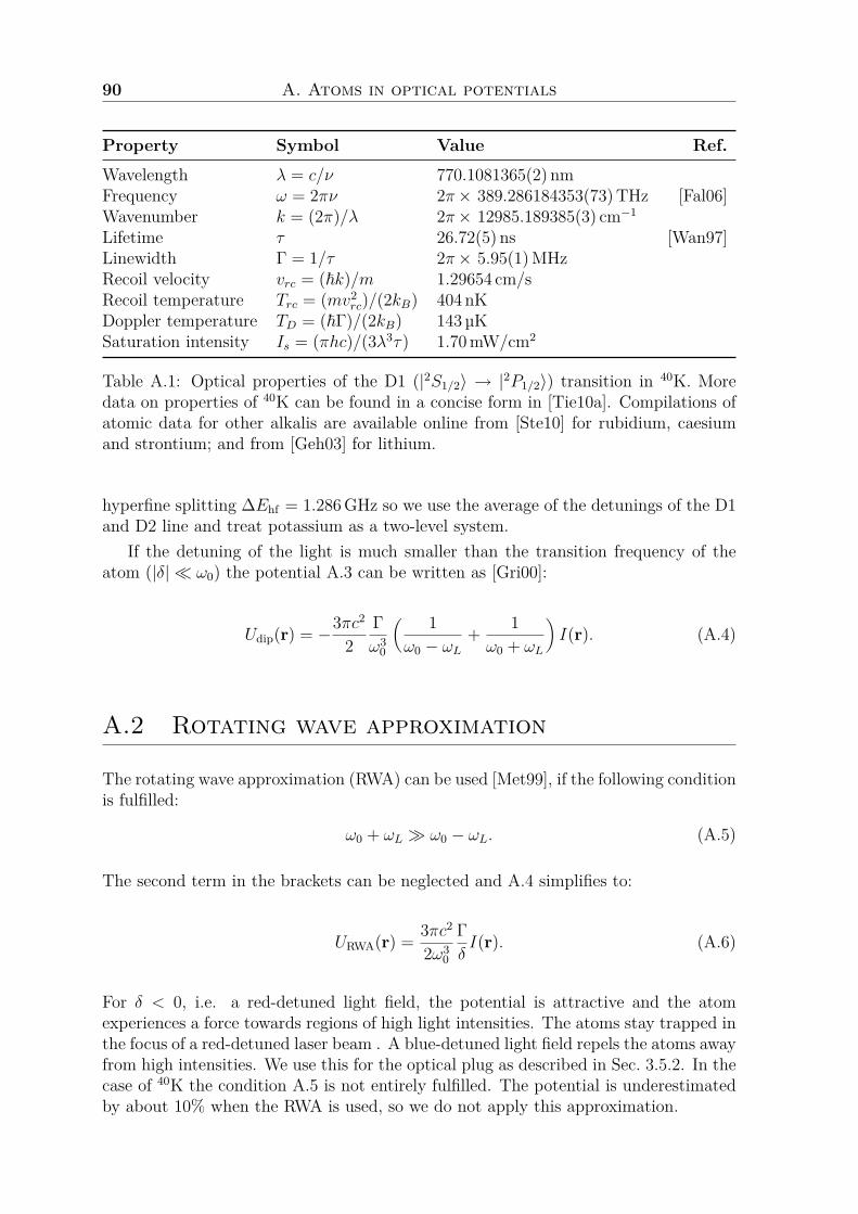
90 A. Atoms in optical potentials
Property Symbol Value Ref.
Wavelength λ = c/ν 770.1081365(2) nmFrequency ω = 2πν 2π× 389.286184353(73)THz [Fal06]Wavenumber k = (2π)/λ 2π× 12985.189385(3) cm−1
Lifetime τ 26.72(5) ns [Wan97]Linewidth Γ = 1/τ 2π× 5.95(1)MHzRecoil velocity vrc = (~k)/m 1.29654 cm/sRecoil temperature Trc = (mv2
rc)/(2kB) 404 nKDoppler temperature TD = (~Γ)/(2kB) 143µKSaturation intensity Is = (πhc)/(3λ3τ) 1.70mW/cm2
Table A.1: Optical properties of the D1 (|2S1/2〉 → |2P1/2〉) transition in 40K. Moredata on properties of 40K can be found in a concise form in [Tie10a]. Compilations ofatomic data for other alkalis are available online from [Ste10] for rubidium, caesiumand strontium; and from [Geh03] for lithium.
hyperfine splitting ∆Ehf = 1.286GHz so we use the average of the detunings of the D1and D2 line and treat potassium as a two-level system.
If the detuning of the light is much smaller than the transition frequency of theatom (|δ| ω0) the potential A.3 can be written as [Gri00]:
Udip(r) = −3πc2
2Γω3
0
( 1ω0 − ωL
+ 1ω0 + ωL
)I(r). (A.4)
A.2 Rotating wave approximation
The rotating wave approximation (RWA) can be used [Met99], if the following conditionis fulfilled:
ω0 + ωL ω0 − ωL. (A.5)
The second term in the brackets can be neglected and A.4 simplifies to:
URWA(r) = 3πc2
2ω30
ΓδI(r). (A.6)
For δ < 0, i.e. a red-detuned light field, the potential is attractive and the atomexperiences a force towards regions of high light intensities. The atoms stay trapped inthe focus of a red-detuned laser beam . A blue-detuned light field repels the atoms awayfrom high intensities. We use this for the optical plug as described in Sec. 3.5.2. In thecase of 40K the condition A.5 is not entirely fulfilled. The potential is underestimatedby about 10% when the RWA is used, so we do not apply this approximation.
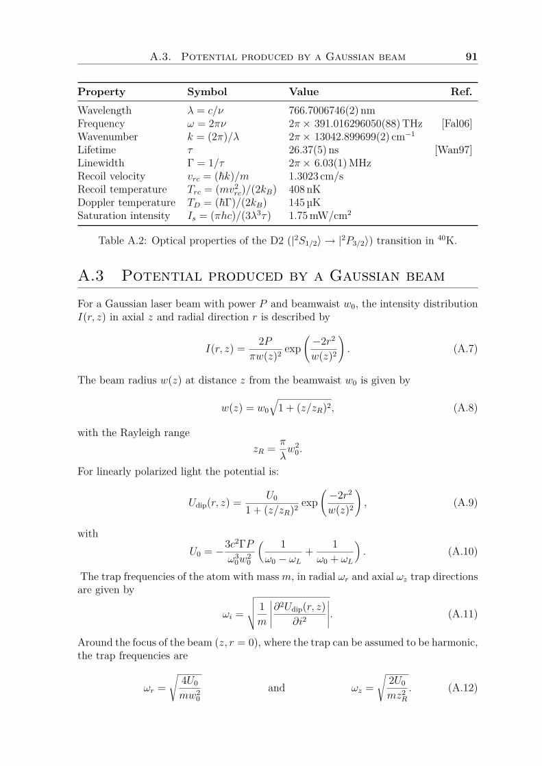
A.3. Potential produced by a Gaussian beam 91
Property Symbol Value Ref.
Wavelength λ = c/ν 766.7006746(2) nmFrequency ω = 2πν 2π× 391.016296050(88)THz [Fal06]Wavenumber k = (2π)/λ 2π× 13042.899699(2) cm−1
Lifetime τ 26.37(5) ns [Wan97]Linewidth Γ = 1/τ 2π× 6.03(1)MHzRecoil velocity vrc = (~k)/m 1.3023 cm/sRecoil temperature Trc = (mv2
rc)/(2kB) 408 nKDoppler temperature TD = (~Γ)/(2kB) 145 µKSaturation intensity Is = (πhc)/(3λ3τ) 1.75mW/cm2
Table A.2: Optical properties of the D2 (|2S1/2〉 → |2P3/2〉) transition in 40K.
A.3 Potential produced by a Gaussian beamFor a Gaussian laser beam with power P and beamwaist w0, the intensity distributionI(r, z) in axial z and radial direction r is described by
I(r, z) = 2Pπw(z)2 exp
(−2r2
w(z)2
). (A.7)
The beam radius w(z) at distance z from the beamwaist w0 is given by
w(z) = w0
√1 + (z/zR)2, (A.8)
with the Rayleigh rangezR = π
λw2
0.
For linearly polarized light the potential is:
Udip(r, z) = U0
1 + (z/zR)2 exp(−2r2
w(z)2
), (A.9)
withU0 = −3c2ΓP
ω30w
20
( 1ω0 − ωL
+ 1ω0 + ωL
). (A.10)
The trap frequencies of the atom with massm, in radial ωr and axial ωz trap directionsare given by
ωi =
√√√√ 1m
∣∣∣∣∣∂2Udip(r, z)∂i2
∣∣∣∣∣. (A.11)
Around the focus of the beam (z, r = 0), where the trap can be assumed to be harmonic,the trap frequencies are
ωr =√
4U0
mw20
and ωz =√
2U0
mz2R
. (A.12)
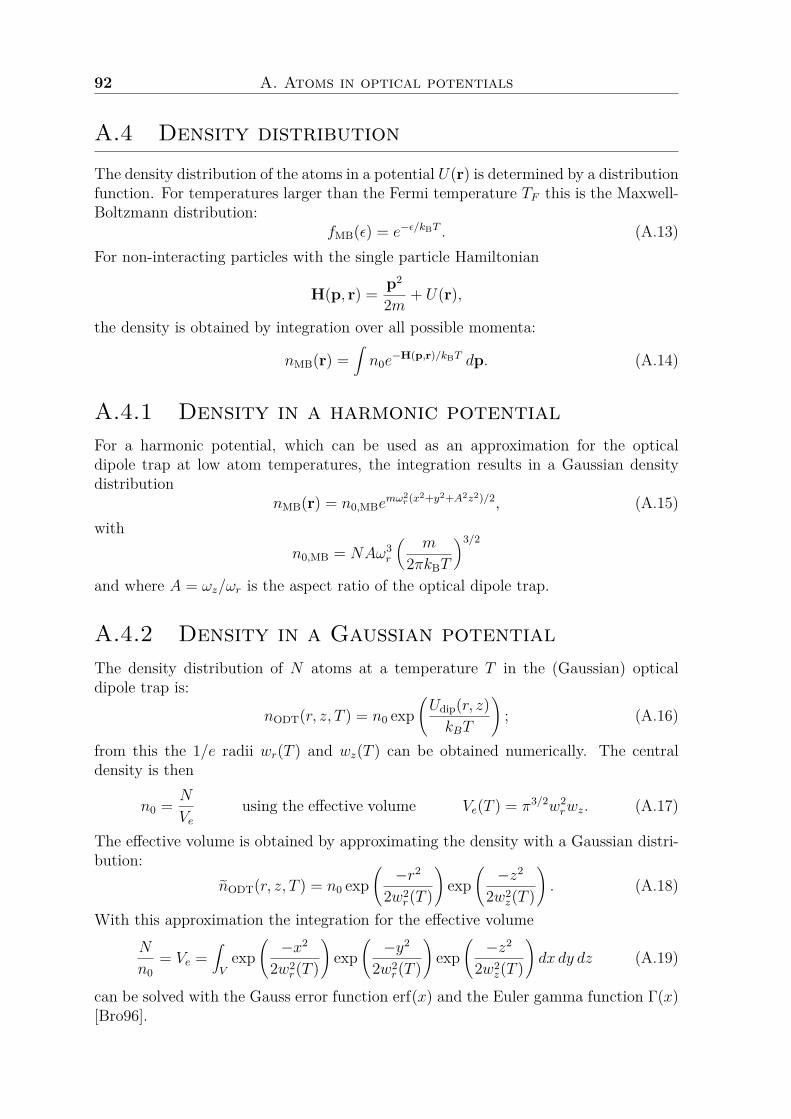
92 A. Atoms in optical potentials
A.4 Density distributionThe density distribution of the atoms in a potential U(r) is determined by a distributionfunction. For temperatures larger than the Fermi temperature TF this is the Maxwell-Boltzmann distribution:
fMB(ε) = e−ε/kBT . (A.13)For non-interacting particles with the single particle Hamiltonian
H(p, r) = p2
2m + U(r),
the density is obtained by integration over all possible momenta:
nMB(r) =∫n0e
−H(p,r)/kBT dp. (A.14)
A.4.1 Density in a harmonic potentialFor a harmonic potential, which can be used as an approximation for the opticaldipole trap at low atom temperatures, the integration results in a Gaussian densitydistribution
nMB(r) = n0,MBemω2r(x2+y2+A2z2)/2, (A.15)
withn0,MB = NAω3
r
(m
2πkBT
)3/2
and where A = ωz/ωr is the aspect ratio of the optical dipole trap.
A.4.2 Density in a Gaussian potentialThe density distribution of N atoms at a temperature T in the (Gaussian) opticaldipole trap is:
nODT(r, z, T ) = n0 exp(Udip(r, z)kBT
); (A.16)
from this the 1/e radii wr(T ) and wz(T ) can be obtained numerically. The centraldensity is then
n0 = N
Veusing the effective volume Ve(T ) = π3/2w2
rwz. (A.17)
The effective volume is obtained by approximating the density with a Gaussian distri-bution:
nODT(r, z, T ) = n0 exp(−r2
2w2r(T )
)exp
(−z2
2w2z(T )
). (A.18)
With this approximation the integration for the effective volumeN
n0= Ve =
∫V
exp(−x2
2w2r(T )
)exp
(−y2
2w2r(T )
)exp
(−z2
2w2z(T )
)dx dy dz (A.19)
can be solved with the Gauss error function erf(x) and the Euler gamma function Γ(x)[Bro96].
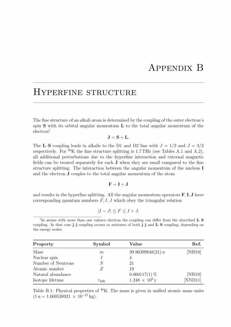
Appendix B
Hyperfine structure
The fine structure of an alkali atom is determined by the coupling of the outer electron’sspin S with its orbital angular momentum L to the total angular momentum of theelectron†
J = S + L.
The L–S coupling leads in alkalis to the D1 and D2 line with J = 1/2 and J = 3/2respectively. For 40K the fine structure splitting is 1.7THz (see Tables A.1 and A.2),all additional perturbations due to the hyperfine interaction and external magneticfields can be treated separately for each J when they are small compared to the finestructure splitting. The interaction between the angular momentum of the nucleus Iand the electron J couples to the total angular momentum of the atom
F = I + J
and results in the hyperfine splitting. All the angular momentum operators F, I,J havecorresponding quantum numbers F, I, J which obey the triangular relation
|I − J | ≤ F ≤ I + J,
†In atoms with more than one valence electron the coupling can differ from the described L–Scoupling. In that case j–j coupling occurs or mixtures of both j–j and L–S coupling, depending onthe energy scales.
Property Symbol Value Ref.
Mass m 39.96399848(21) u [NIS10]Nuclear spin I 4Number of Neutrons N 21Atomic number Z 19Natural abundance 0.000117(1)% [NIS10]Isotope lifetime τ40K 1.248 × 10⁹ y [NND11]
Table B.1: Physical properties of 40K. The mass is given in unified atomic mass units(1 u = 1.660538921 × 10⁻²⁷ kg).
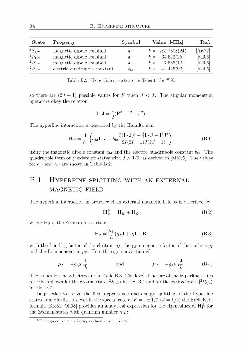
94 B. Hyperfine structure
State Property Symbol Value [MHz] Ref.2S1/2 magnetic dipole constant ahf h×−285.7308(24) [Ari77]2P1/2 magnetic dipole constant ahf h× −34.523(25) [Fal06]2P3/2 magnetic dipole constant ahf h× −7.585(10) [Fal06]2P3/2 electric quadrupole constant bhf h× −3.445(90) [Fal06]
Table B.2: Hyperfine structure coefficients for 40K.
so there are (2J + 1) possible values for F when J < I. The angular momentumoperators obey the relation
I · J = 12(F2 − I2 − J2).
The hyperfine interaction is described by the Hamiltonian
Hhf = 1~2
(ahfI · J + bhf
3(I · J)2 + 32I · J− I2J2
2I(2I − 1)J(2J − 1)
), (B.1)
using the magnetic dipole constant ahf and the electric quadrupole constant bhf . Thequadrupole term only exists for states with J > 1/2, as derived in [MK85]. The valuesfor ahf and bhf are shown in Table B.2.
B.1 Hyperfine splitting with an externalmagnetic field
The hyperfine interaction in presence of an external magnetic field B is described by
HBhf = Hhf + HZ, (B.2)
where HZ is the Zeeman interaction
HZ = µB
~(gJJ + gII) ·B, (B.3)
with the Landé g-factor of the electron gJ , the gyromagnetic factor of the nucleus gIand the Bohr magneton µB. Here the sign convention is‡:
µI = −gIµBI~
and µJ = −gJµBJ~. (B.4)
The values for the g-factors are in Table B.3. The level structure of the hyperfine statesfor 40K is shown for the ground state |2S1/2〉 in Fig. B.1 and for the excited state |2P3/2〉in Fig. B.2.
In practice we solve the field dependence and energy splitting of the hyperfinestates numerically, however in the special case of F = I±1/2 (J = 1/2) the Breit-Rabiformula [Bre31, Oh08] provides an analytical expression for the eigenvalues of HB
hf forthe Zeeman states with quantum number mF :
‡The sign convention for µI is chosen as in [Ari77].
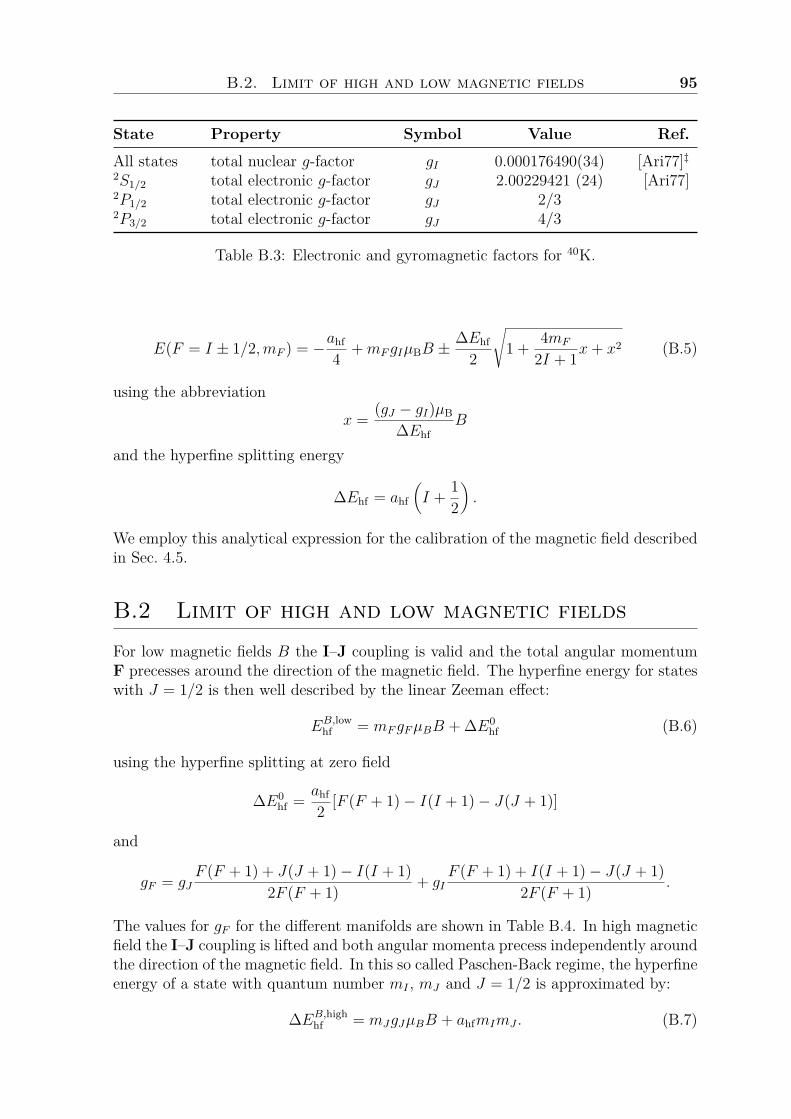
B.2. Limit of high and low magnetic fields 95
State Property Symbol Value Ref.
All states total nuclear g-factor gI 0.000176490(34) [Ari77]‡2S1/2 total electronic g-factor gJ 2.00229421 (24) [Ari77]2P1/2 total electronic g-factor gJ 2/32P3/2 total electronic g-factor gJ 4/3
Table B.3: Electronic and gyromagnetic factors for 40K.
E(F = I ± 1/2,mF ) = −ahf
4 +mFgIµBB ±∆Ehf
2
√1 + 4mF
2I + 1x+ x2 (B.5)
using the abbreviationx = (gJ − gI)µB
∆EhfB
and the hyperfine splitting energy
∆Ehf = ahf
(I + 1
2
).
We employ this analytical expression for the calibration of the magnetic field describedin Sec. 4.5.
B.2 Limit of high and low magnetic fieldsFor low magnetic fields B the I–J coupling is valid and the total angular momentumF precesses around the direction of the magnetic field. The hyperfine energy for stateswith J = 1/2 is then well described by the linear Zeeman effect:
EB,lowhf = mFgFµBB + ∆E0
hf (B.6)
using the hyperfine splitting at zero field
∆E0hf = ahf
2 [F (F + 1)− I(I + 1)− J(J + 1)]
and
gF = gJF (F + 1) + J(J + 1)− I(I + 1)
2F (F + 1) + gIF (F + 1) + I(I + 1)− J(J + 1)
2F (F + 1) .
The values for gF for the different manifolds are shown in Table B.4. In high magneticfield the I–J coupling is lifted and both angular momenta precess independently aroundthe direction of the magnetic field. In this so called Paschen-Back regime, the hyperfineenergy of a state with quantum number mI , mJ and J = 1/2 is approximated by:
∆EB,highhf = mJgJµBB + ahfmImJ . (B.7)
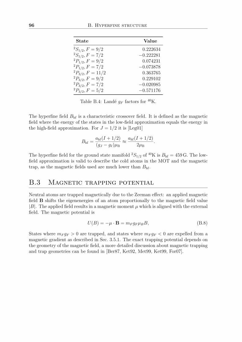
96 B. Hyperfine structure
State Value2S1/2, F = 9/2 0.2226342S1/2, F = 7/2 −0.2222812P1/2, F = 9/2 0.0742312P1/2, F = 7/2 −0.0738782P3/2, F = 11/2 0.3637652P3/2, F = 9/2 0.2291022P3/2, F = 7/2 −0.0209852P3/2, F = 5/2 −0.571176
Table B.4: Landé gF factors for 40K.
The hyperfine field Bhf is a characteristic crossover field. It is defined as the magneticfield where the energy of the states in the low-field approximation equals the energy inthe high-field approximation. For J = 1/2 it is [Leg01]
Bhf = ahf(I + 1/2)(gJ − gI)µB
≈ ahf(I + 1/2)2µB
.
The hyperfine field for the ground state manifold 2S1/2 of 40K is Bhf = 459G. The low-field approximation is valid to describe the cold atoms in the MOT and the magnetictrap, as the magnetic fields used are much lower than Bhf .
B.3 Magnetic trapping potentialNeutral atoms are trapped magnetically due to the Zeeman effect: an applied magneticfield B shifts the eigenenergies of an atom proportionally to the magnetic field value|B|. The applied field results in a magnetic moment µ which is aligned with the externalfield. The magnetic potential is
U(B) = −µ ·B = mFgFµBB, (B.8)
States where mFgF > 0 are trapped, and states where mFgF < 0 are expelled from amagnetic gradient as described in Sec. 3.5.1. The exact trapping potential depends onthe geometry of the magnetic field, a more detailed discussion about magnetic trappingand trap geometries can be found in [Ber87, Ket92, Met99, Ket99, For07].
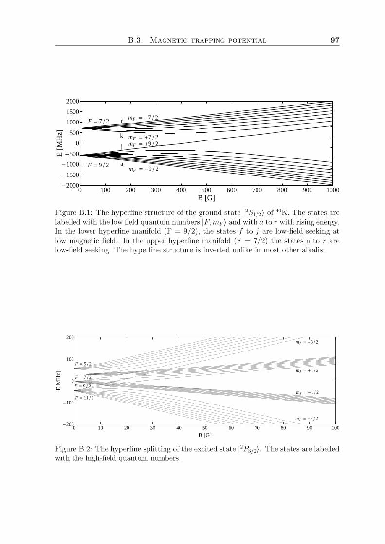
B.3. Magnetic trapping potential 97
F = 9 2
F = 7 2
a
j
r
k
mF = -9 2
mF = +9 2
mF = -7 2
mF = +7 2
0 100 200 300 400 500 600 700 800 900 1000-2000
-1500
-1000
-500
0
500
1000
1500
2000
B @GD
E@M
HzD
Figure B.1: The hyperfine structure of the ground state |2S1/2〉 of 40K. The states arelabelled with the low field quantum numbers |F,mF 〉 and with a to r with rising energy.In the lower hyperfine manifold (F = 9/2), the states f to j are low-field seeking atlow magnetic field. In the upper hyperfine manifold (F = 7/2) the states o to r arelow-field seeking. The hyperfine structure is inverted unlike in most other alkalis.
mJ = -1 2
mJ = +1 2
mJ = -3 2
mJ = +3 2
F = 11 2
F = 9 2
F = 7 2
F = 5 2
0 10 20 30 40 50 60 70 80 90 100-200
-100
0
100
200
B @GD
E@M
HzD
Figure B.2: The hyperfine splitting of the excited state |2P3/2〉. The states are labelledwith the high-field quantum numbers.

Appendix C
Optical transition probabilities
When imaging cold atoms, the transition strength of the used imaging transition needsto be known to accurately fit the number of atoms. Additionally the frequency of theimaging light and – if necessary – of the repump light has to be chosen according to thepossible transitions and decay channels. The transition matrix element µeg describesthe coupling between a ground and an excited state by an electric dipole:
µeg = e 〈e|ε · r|g〉 ,
here ε is the unit vector of the light polarization and e the elementary charge. Thestates are described by a wavefunction which can be factorised into a radial part andan angular part. The transition matrix element can be expanded in terms of Clebsch-Gordan coefficients using the Wigner-Eckart theorem. A detailed derivation can befound for example in [Met99, Wal10, LeB11]. The transition strengths for other isotopesof potassium and other alkalis are in listed [Met99].
C.1 Transition probabilities at zero magneticfield
The transition matrix element µeg coupling a ground state with quantum numbersn, L, S, I, J, F,mF to an excited state with quantum numbers n, L′, S, I, J ′, F ′,m′F canbe expressed as:
µeg = eRA,the radial part R only concerns the n, L quantum numbers and is the same for alltransitions within one line. To compare the transition strengths of transitions in theD1 and in the D2 line, the radial part R has to be taken into account (see [Met99]).The angular part is described by:
A = (−1)1+L′+S+J+J ′+I−m′√
(2J + 1)(2J ′ + 1)(2F + 1)(2F ′ + 1)
×√
max(L,L′)(F 1 F ′
m q −m′)
J ′ F ′ IF J 1
L′ J ′ SJ L 1
. (C.1)
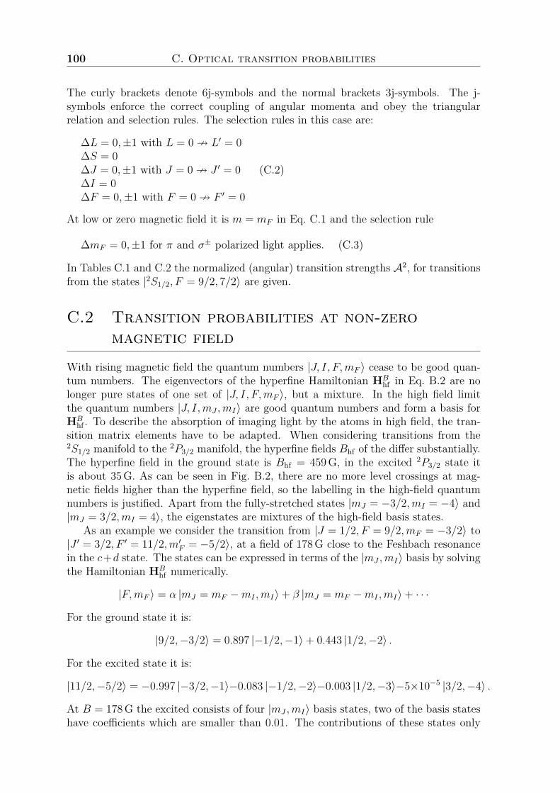
100 C. Optical transition probabilities
The curly brackets denote 6j-symbols and the normal brackets 3j-symbols. The j-symbols enforce the correct coupling of angular momenta and obey the triangularrelation and selection rules. The selection rules in this case are:
∆L = 0,±1 with L = 0 9 L′ = 0∆S = 0∆J = 0,±1 with J = 0 9 J ′ = 0∆I = 0∆F = 0,±1 with F = 0 9 F ′ = 0
(C.2)
At low or zero magnetic field it is m = mF in Eq. C.1 and the selection rule
∆mF = 0,±1 for π and σ± polarized light applies. (C.3)
In Tables C.1 and C.2 the normalized (angular) transition strengths A2, for transitionsfrom the states |2S1/2, F = 9/2, 7/2〉 are given.
C.2 Transition probabilities at non-zeromagnetic field
With rising magnetic field the quantum numbers |J, I, F,mF 〉 cease to be good quan-tum numbers. The eigenvectors of the hyperfine Hamiltonian HB
hf in Eq. B.2 are nolonger pure states of one set of |J, I, F,mF 〉, but a mixture. In the high field limitthe quantum numbers |J, I,mJ ,mI〉 are good quantum numbers and form a basis forHB
hf . To describe the absorption of imaging light by the atoms in high field, the tran-sition matrix elements have to be adapted. When considering transitions from the2S1/2 manifold to the 2P3/2 manifold, the hyperfine fields Bhf of the differ substantially.The hyperfine field in the ground state is Bhf = 459G, in the excited 2P3/2 state itis about 35G. As can be seen in Fig. B.2, there are no more level crossings at mag-netic fields higher than the hyperfine field, so the labelling in the high-field quantumnumbers is justified. Apart from the fully-stretched states |mJ = −3/2,mI = −4〉 and|mJ = 3/2,mI = 4〉, the eigenstates are mixtures of the high-field basis states.
As an example we consider the transition from |J = 1/2, F = 9/2,mF = −3/2〉 to|J ′ = 3/2, F ′ = 11/2,m′F = −5/2〉, at a field of 178G close to the Feshbach resonancein the c+d state. The states can be expressed in terms of the |mJ ,mI〉 basis by solvingthe Hamiltonian HB
hf numerically.
|F,mF 〉 = α |mJ = mF −mI ,mI〉+ β |mJ = mF −mI ,mI〉+ · · ·
For the ground state it is:
|9/2,−3/2〉 = 0.897 |−1/2,−1〉+ 0.443 |1/2,−2〉 .
For the excited state it is:
|11/2,−5/2〉 = −0.997 |−3/2,−1〉−0.083 |−1/2,−2〉−0.003 |1/2,−3〉−5×10−5 |3/2,−4〉 .
At B = 178G the excited consists of four |mJ ,mI〉 basis states, two of the basis stateshave coefficients which are smaller than 0.01. The contributions of these states only

C.2. Transition probabilities at non-zero magnetic field 101
F=
9/2,
mF
=−
9/2
−7/
2−
5/2
−3/
2−
1/2
1/2
3/2
5/2
7/2
9/2
ab
cd
ef
gh
ij
πF′=
9/2
8149
259
11
925
4981
F′=
7/2
032
5672
8080
7256
32σ
+F′=
9/2
1832
4248
5048
4232
18F′=
7/2
144
112
8460
4024
124
F=
7/2,
mF
=−
7/2
−5/
2−
3/2
−1/
21/
23/
25/
27/
2r
qp
on
ml
k
πF′=
9/2
3256
7280
8072
5632
F′=
7/2
4925
91
19
2549
σ+
F′=
9/2
412
2440
6084
112
144
F′=
7/2
1424
3032
3024
14
TableC.1:(
Ang
ular)t
ransition
streng
thsfrom|F
=7/
2,F
=9/
2,mF〉t
othe
2 P1/
2man
ifold
(D1-lin
e)in
40K.T
hevalues
areno
rmal-
ized
tothewe
akestt
ransition
intheD1lin
e(|F
=9/
2,mF
=−
1/2〉→|F′=
9/2,m′ F
=−
1/2〉).
Itism′ F
=mF
+1forσ
+tran
sitions
andm′ F
=mFforπtran
sitions.

102 C. Optical transition probabilities
F=
9/2,m
F=
−9/2
−7/2
−5/2
−3/2
−1/2
1/2
3/2
5/2
7/2
9/2
ab
cd
ef
gh
ij
F′=
11/268040
122472163296
190512204120
204120190512
163296122472
68040π
F′=
9/2181440
10976056000
201602240
224020160
56000109760
181440F′=
7/217248
3018438808
4312043120
3880830184
17248F′=
11/26804
2041240824
68040102060
142884190512
244944306180
374220σ
+F′=
9/240320
7168094080
107520112000
10752094080
7168040320
F′=
7/277616
6036845276
3234021560
129366468
2156F
=7/2,m
F=
−7/2
−5/2
−3/2
−1/2
1/2
3/2
5/2
7/2
rq
po
nm
lk
F′=
9/233880
5929076230
8470084700
7623059290
33880π
F′=
7/2215600
11000039600
44004400
39600110000
215600F′=
5/280190
133650160380
160380133650
80190F′=
9/24235
1270525410
4235063525
88935118580
152460σ
+F′=
7/261600
105600132000
140800132000
10560061600
F′=
5/2280665
200475133650
8019040095
13365
TableC.2:
(Angular)
transitionstrengths
from| 2S
1/2 ,F
=7/2,F
=9/2,m
F 〉to
the2P
3/2
manifold
(D2-line)
for40K
.The
valuesare
normalized
tothe
weakesttransition
inthe
D2line
(|F=
9/2,mF
=−
1/2〉→|F′=
9/2,m′F
=−
1/2〉)and
multiplied
with
thegreatest
common
denominator
toobtain
integervalues
asit
isdone
in[M
et99].It
ism′F
=mF
+1for
σ+transitions
andm′F
=mF
forπtransitions.
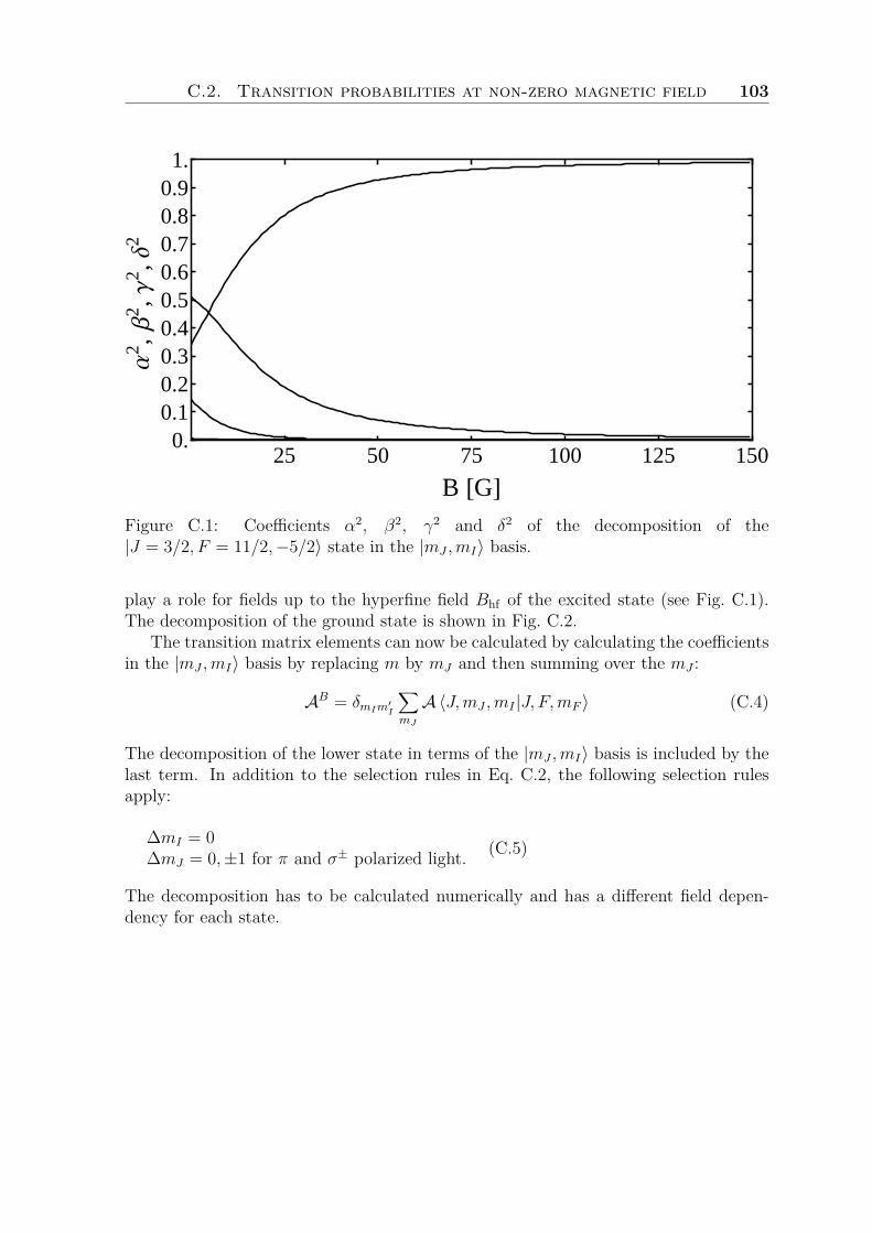
C.2. Transition probabilities at non-zero magnetic field 103
25 50 75 100 125 1500.
0.10.20.30.40.50.60.70.80.9
1.
B @GD
Α2 ,
Β2 ,Γ
2 ,∆2
Figure C.1: Coefficients α2, β2, γ2 and δ2 of the decomposition of the|J = 3/2, F = 11/2,−5/2〉 state in the |mJ ,mI〉 basis.
play a role for fields up to the hyperfine field Bhf of the excited state (see Fig. C.1).The decomposition of the ground state is shown in Fig. C.2.
The transition matrix elements can now be calculated by calculating the coefficientsin the |mJ ,mI〉 basis by replacing m by mJ and then summing over the mJ :
AB = δmIm′I∑mJ
A〈J,mJ ,mI |J, F,mF 〉 (C.4)
The decomposition of the lower state in terms of the |mJ ,mI〉 basis is included by thelast term. In addition to the selection rules in Eq. C.2, the following selection rulesapply:
∆mI = 0∆mJ = 0,±1 for π and σ± polarized light. (C.5)
The decomposition has to be calculated numerically and has a different field depen-dency for each state.
104 C. Optical transition probabilities
100 200 300 400 500 600 700 800 900 10000.
0.10.20.30.40.50.60.70.80.9
1.
B @GD
Α2 ,
Β2
Figure C.2: Coefficients α2 and β2 of the decomposition of the|J = 1/2, F = 9/2,−3/2〉 state in the |mJ ,mI〉 basis.
Bibliography
[A] All data from internet sources was retrieved in the year noted.[Ada95] C. S. Adams, H. J. Lee, N. Davidson, M. Kasevich and S. Chu, Evaporative
Cooling in a Crossed Dipole Trap, Phys. Rev. Lett. 74, 3577 (1995).[And95] M. H. Anderson, J. R. Ensher, M. R. Matthews, C. E. Wieman and E. A.
Cornell, Observation of Bose-Einstein Condensation in a Dilute AtomicVapor , Science 269, 198 (1995).
[Ari77] E. Arimondo, M. Inguscio and P. Violino, Experimental determinations of thehyperfine structure in the alkali atoms, Rev. Mod. Phys. 49, 31 (1977).
[Ash70] A. Ashkin, Acceleration and Trapping of Particles by Radiation Pressure,Phys. Rev. Lett. 24, 156 (1970).
[Aub05] S. Aubin, M. H. T. Extavour, S. Myrskog, L. J. LeBlanc, J. Estève, S. Singh,P. Scrutton, D. McKay, R. McKenzie, I. D. Leroux, A. Stummer andJ. H. Thywissen, Trapping Fermionic 40K and Bosonic 87Rb on a Chip,Journal of Low Temperature Physics 140, 377 (2005).
[Bag87] V. Bagnato, D. E. Pritchard and D. Kleppner, Bose-Einstein condensationin an external potential, Phys. Rev. A 35, 4354 (1987).
[Bar02] M. Baranov, L. Dobrek, K. Góral, L. Santos and M. Lewenstein, UltracoldDipolar Gases - a Challenge for Experiments and Theory, Physica Scripta2002, 74 (2002).
[Ber87] T. Bergeman, G. Erez and H. J. Metcalf, Magnetostatic trapping fields forneutral atoms, Phys. Rev. A 35, 1535 (1987).
[Bil08] J. Billy, V. Josse, Z. Zuo, A. Bernard, B. Hambrecht, P. Lugan, D. Clement,L. Sanchez-Palencia, P. Bouyer and A. Aspect, Direct observation of An-derson localization of matter waves in a controlled disorder , Nature 453,891 (2008).
[Bir74] F. Biraben, B. Cagnac and G. Grynberg, Experimental Evidence of Two-Photon Transition without Doppler Broadening, Phys. Rev. Lett. 32, 643(1974).
[Blo08] I. Bloch, J. Dalibard andW. Zwerger,Many-body physics with ultracold gases,Rev. Mod. Phys. 80, 885 (2008).
[Boh99] J. L. Bohn and P. S. Julienne, Semianalytic theory of laser-assisted resonantcold collisions, Phys. Rev. A 60, 414 (1999).
106 Bibliography
[Bos24] S. N. Bose, Plancks Gesetz und Lichtquantenhypothese, Zeitschrift für Physik26, 178 (1924).
[Bre31] G. Breit and I. I. Rabi, Measurement of Nuclear Spin, Phys. Rev. 38, 2082(1931).
[Bro96] I. N. Bronstein, K. A. Semandjajew, W. Hackbusch, H. R. Schwarz andE. Zeidler, Taschenbuch der Mathematik (Teubner, Stuttgart, 1996).
[Bru00] G. M. Bruun and C. W. Clark, Ideal gases in time-dependent traps, Phys.Rev. A 61, 061601 (2000).
[Bur97] J. P. Burke, J. L. Bohn, B. D. Esry and C. H. Greene, Impact of the 87Rbsinglet scattering length on suppressing inelastic collisions, Phys. Rev. A55, R2511 (1997).
[But97] D. A. Butts and D. S. Rokhsar, Trapped Fermi gases, Phys. Rev. A 55, 4346(1997).
[Cas96] Y. Castin and R. Dum, Bose-Einstein Condensates in Time DependentTraps, Phys. Rev. Lett. 77, 5315 (1996).
[Cat98] F. S. Cataliotti, E. A. Cornell, C. Fort, M. Inguscio, F. Marin, M. Prevedelli,L. Ricci and G. M. Tino,Magneto-optical trapping of Fermionic potassiumatoms, Phys. Rev. A 57, 1136 (1998).
[Cat06] J. Catani, P. Maioli, L. De Sarlo, F. Minardi and M. Inguscio, Intense slowbeams of bosonic potassium isotopes, Phys. Rev. A 73, 033415 (2006).
[Cha06] S. Chaudhuri, S. Roy and C. S. Unnikrishnan, Realization of an intensecold Rb atomic beam based on a two-dimensional magneto-optical trap:Experiments and comparison with simulations, Phys. Rev. A 74, 023406(2006).
[Che05] Q. Chen, J. Stajic, S. Tan and K. Levin, BCS - BEC crossover: Fromhigh temperature superconductors to ultracold superfluids, Physics Reports412, 1 (2005).
[Chi05] C. Chin, A simple model of Feshbach molecules, ArXiv e-prints 0506.313(2005).
[Chi10] C. Chin, R. Grimm, P. Julienne and E. Tiesinga, Feshbach resonances inultracold gases, Rev. Mod. Phys. 82, 1225 (2010).
[Chu86] S. Chu, J. E. Bjorkholm, A. Ashkin and A. Cable, Experimental Observationof Optically Trapped Atoms, Phys. Rev. Lett. 57, 314 (1986).
[Cou98] P. Courteille, R. S. Freeland, D. J. Heinzen, F. A. van Abeelen and B. J.Verhaar, Observation of a Feshbach Resonance in Cold Atom Scattering,Phys. Rev. Lett. 81, 69 (1998).
[CT77] C. Cohen-Tannoudji, B. Diu and F. Laloe, Quantum mechanics (Wiley, NewYork, 1977).
[Dav95a] K. B. Davis, M. O. Mewes, M. R. Andrews, N. J. van Druten, D. S. Durfee,D. M. Kurn and W. Ketterle, Bose-Einstein Condensation in a Gas ofSodium Atoms, Phys. Rev. Lett. 75, 3969 (1995).
Bibliography 107
[Dav95b] K. B. Davis, M. O. Mewes and W. Ketterle, An analytical model for evap-orative cooling of atoms, Applied Physics B: Lasers and Optics 60, 155(1995).
[Deh10] B. Deh, W. Gunton, B. G. Klappauf, Z. Li, M. Semczuk, J. Van Dongen andK. W. Madison, Giant Feshbach resonances in 6Li-85Rb mixtures, Phys.Rev. A 82, 020701 (2010).
[DeM99a] B. DeMarco and D. S. Jin, Onset of Fermi Degeneracy in a Trapped AtomicGas, Science 285, 1703 (1999).
[DeM99b] B. DeMarco, H. Rohner and D. S. Jin, An enriched 40K source for fermionicatom studies, Review of Scientific Instruments 70, 1967 (1999).
[DeM01] B. DeMarco, Quantum Behavior of an Atomic Fermi Gas, Ph.D. thesis, Uni-versity of Colorado (2001).
[Deu98] I. H. Deutsch and P. S. Jessen, Quantum-state control in optical lattices,Phys. Rev. A 57, 1972 (1998).
[Die98] K. Dieckmann, R. J. C. Spreeuw, M. Weidemüller and J. T. M. Walraven,Two-dimensional magneto-optical trap as a source of slow atoms, Phys.Rev. A 58, 3891 (1998).
[Dir26] P. A. M. Dirac, On the Theory of Quantum Mechanics, Proceedings of theRoyal Society of London. Series A, Containing Papers of a Mathematicaland Physical Character 112, pp. 661 (1926).
[Efi70] V. Efimov, Energy levels arising from resonant two-body forces in a three-bodysystem, Physics Letters B 33, 563 (1970).
[Ein25] A. Einstein, Quantentheorie des einatomigen idealen Gases, 2. Abhandlung,Sitzungsberichte der Preussischen Akademie der Wissenschaften zu Berlinpages 3–14 (1925).
[Ekl75] H. Eklund, A. Roos and S. T. Eng, Rotation of laser beam polarization inacousto-optic devices, Optical and Quantum Electronics 7, 73 (1975).
[Fal06] S. Falke, E. Tiemann, C. Lisdat, H. Schnatz and G. Grosche, Transition fre-quencies of the D lines of 39K, 40K, and 41K measured with a femtosecondlaser frequency comb, Phys. Rev. A 74, 032503 (2006).
[Fal08] S. Falke, H. Knöckel, J. Friebe, M. Riedmann, E. Tiemann and C. Lisdat,Potassium ground-state scattering parameters and Born-Oppenheimer po-tentials from molecular spectroscopy, Phys. Rev. A 78, 012503 (2008).
[Fed96] P. O. Fedichev, Y. Kagan, G. V. Shlyapnikov and J. T. M. Walraven,Influence of Nearly Resonant Light on the Scattering Length in Low-Temperature Atomic Gases, Phys. Rev. Lett. 77, 2913 (1996).
[Fer24] E. Fermi, Über die Wahrscheinlichkeit der Quantenzustände, Zeitschrift fürPhysik A Hadrons and Nuclei 26, 54 (1924).
[Fer26] E. Fermi, Zur Quantelung des idealen einatomigen Gases, Zeitschrift fürPhysik A Hadrons and Nuclei 36, 902 (1926), a translation into Englishof the original report by A. Zannoni: ArXiv e-prints 9912.229(1999).
108 Bibliography
[Fer02] G. Ferrari, M. Inguscio, W. Jastrzebski, G. Modugno, G. Roati and A. Si-moni, Collisional Properties of Ultracold K-Rb Mixtures, Phys. Rev. Lett.89, 053202 (2002).
[Fer06] F. Ferlaino, C. D’Errico, G. Roati, M. Zaccanti, M. Inguscio, G. Modugnoand A. Simoni, Feshbach spectroscopy of a K−Rb atomic mixture, Phys.Rev. A 73, 040702 (2006).
[Fes58] H. Feshbach, Unified theory of nuclear reactions, Annals of Physics 5, 357(1958).
[Fes62] H. Feshbach, A unified theory of nuclear reactions. II , Annals of Physics 19,287 (1962).
[Fey82] R. Feynman, Simulating physics with computers, International Journal ofTheoretical Physics 21, 467 (1982).
[Fla99] V. V. Flambaum, G. F. Gribakin and C. Harabati, Analytical calculation ofcold-atom scattering, Phys. Rev. A 59, 1998 (1999).
[Fli91] T. Fließbach, Quantenmechanik (BI Wissenschaftlicher Verlag, Mannheim,1991).
[For07] J. Fortágh and C. Zimmermann, Magnetic microtraps for ultracold atoms,Rev. Mod. Phys. 79, 235 (2007).
[Gae07] J. P. Gaebler, J. T. Stewart, J. L. Bohn and D. S. Jin, p-Wave FeshbachMolecules, Phys. Rev. Lett. 98, 200403 (2007).
[Gao05] B. Gao, E. Tiesinga, C. J. Williams and P. S. Julienne, Multichannelquantum-defect theory for slow atomic collisions, Phys. Rev. A 72, 042719(2005).
[Gau10] S. Gautam and D. Angom, Scattering length for fermionic alkali atoms, TheEuropean Physical Journal D - Atomic, Molecular, Optical and PlasmaPhysics 56, 173 (2010).
[Geh98] M. E. Gehm, K. M. O’Hara, T. A. Savard and J. E. Thomas, Dynamics ofnoise-induced heating in atom traps, Phys. Rev. A 58, 3914 (1998).
[Geh03] M. E. Gehm, Properties of 6Li (2003), http://www.phy.duke.edu/research/photon/qoptics/techdocs/pdf/PropertiesOfLi.pdf.
[Gio08] S. Giorgini, L. P. Pitaevskii and S. Stringari, Theory of ultracold atomicFermi gases, Rev. Mod. Phys. 80, 1215 (2008).
[Gün05] K. Günter, T. Stöferle, H. Moritz, M. Köhl and T. Esslinger, p-Wave Interac-tions in Low-Dimensional Fermionic Gases, Phys. Rev. Lett. 95, 230401(2005).
[Goo10] M. R. Goosen, T. G. Tiecke, W. Vassen and S. J. J. M. F. Kokkelmans,Feshbach resonances in 3He∗-4He∗ mixtures, Phys. Rev. A 82, 042713(2010).
[Goz93] A. Gozzini, F. Mango, J. Xu, G. Alzetta, F. Maccarrone and R. Bernheim,Light-induced ejection of alkali atoms in polysiloxane coated cells, Il NuovoCimento D 15, 709 (1993).

Bibliography 109
[Gre01] M. Greiner, I. Bloch, T. W. Hänsch and T. Esslinger, Magnetic transport oftrapped cold atoms over a large distance, Phys. Rev. A 63, 031401 (2001).
[Gre02] M. Greiner, O. Mandel, T. Esslinger, T. W. Hänsch and I. Bloch, Quantumphase transition from a superfluid to a Mott insulator in a gas of ultracoldatoms, Nature (London) 415, 39 (2002).
[Gre03] M. Greiner, C. A. Regal and D. S. Jin, Emergence of a molecular Bose-Einstein condensate from a Fermi gas, Nature (London) 426, 537 (2003).
[Gri93] G. F. Gribakin and V. V. Flambaum, Calculation of the scattering length inatomic collisions using the semiclassical approximation, Phys. Rev. A 48,546 (1993).
[Gri00] R. Grimm, M. Weidemüller and Y. Ovchinnikov, Optical Dipole Traps forNeutral Atoms, Adv. At. Mol. Opt. Phys. 42, 42 (2000).
[Gri05] P. F. Griffin, K. J. Weatherill and C. S. Adams, Fast switching of alkali atomdispensers using laser-induced heating, Review of Scientific Instruments76, 093102 (2005).
[Gus01] T. L. Gustavson, A. P. Chikkatur, A. E. Leanhardt, A. Görlitz, S. Gupta,D. E. Pritchard and W. Ketterle, Transport of Bose-Einstein Condensateswith Optical Tweezers, Phys. Rev. Lett. 88, 020401 (2001).
[Gus08] M. Gustavsson, E. Haller, M. J. Mark, J. G. Danzl, G. Rojas-Kopeinig andH.-C. Nägerl, Control of Interaction-Induced Dephasing of Bloch Oscilla-tions, Phys. Rev. Lett. 100, 080404 (2008).
[Ham10] H.-W. Hammer and L. Platter, Efimov States in Nuclear and ParticlePhysics, Annual Review of Nuclear and Particle Science 60, 207 (2010).
[Han09] T. M. Hanna, E. Tiesinga and P. S. Julienne, Prediction of Feshbach reso-nances from three input parameters, Phys. Rev. A 79, 040701 (2009).
[Han10] T. M. Hanna, E. Tiesinga and P. S. Julienne, Creation and manipulationof Feshbach resonances with radiofrequency radiation, New Journal ofPhysics 12, 083031 (2010).
[Hap72] W. Happer, Optical Pumping, Rev. Mod. Phys. 44, 169 (1972).[Hec90] E. Hecht, Optics (Addison-Wesley, 1990).[Heo11] M.-S. Heo, J.-y. Choi and Y.-i. Shin, Fast production of large 23Na Bose-
Einstein condensates in an optically plugged magnetic quadrupole trap,Phys. Rev. A 83, 013622 (2011).
[Hes86] H. F. Hess, Evaporative cooling of magnetically trapped and compressed spin-polarized hydrogen, Phys. Rev. B 34, 3476 (1986).
[Hut94] J. M. Hutson, Coupled channel methods for solving the bound-stateSchrödinger equation, Comput. Phys. Commun. 84, 1 (1994).
[Hut07] J. M. Hutson, Feshbach resonances in ultracold atomic and molecular colli-sions: threshold behaviour and suppression of poles in scattering lengths,New Journal of Physics 9, 152 (2007).
110 Bibliography
[Ing07] M. Inguscio, W. Ketterle and C. Salomon (Editors), Proceedings of the In-ternational School of Physics "Enrico Fermi", Course CLXIV, Ultra-coldFermi Gases (Società Italiana di Fisica and IOS Press Amsterdam, 2007).
[Ino98] S. Inouye, M. R. Andrews, J. Stenger, H.-J. Miesner, D. M. Stamper-KurnandW. Ketterle, Observation of Feshbach resonances in a Bose – Einsteincondensate, Nature 392, 151 (1998).
[Ino04] S. Inouye, J. Goldwin, M. L. Olsen, C. Ticknor, J. L. Bohn and D. S. Jin, Ob-servation of Heteronuclear Feshbach Resonances in a Mixture of Bosonsand Fermions, Phys. Rev. Lett. 93, 183201 (2004).
[Joc02] S. Jochim, M. Bartenstein, G. Hendl, J. H. Denschlag, R. Grimm, A. Moskand M. Weidemüller, Magnetic Field Control of Elastic Scattering ina Cold Gas of Fermionic Lithium Atoms, Phys. Rev. Lett. 89, 273202(2002).
[Jof93] M. A. Joffe, W. Ketterle, A. Martin and D. E. Pritchard, Transverse coolingand deflection of an atomic beam inside a Zeeman slower , J. Opt. Soc.Am. B 10, 2257 (1993).
[Joh73] B. R. Johnson, The multichannel log-derivative method for scattering calcu-lations, J. Comput. Phys. 13, 445 (1973).
[Jör08] R. Jördens, N. Strohmaier, K. Günter, H. Moritz and T. Esslinger, A Mottinsulator of fermionic atoms in an optical lattice, Nature (London) 455,204 (2008).
[Jör10a] R. Jördens, Metallic and Mott-insulating phases in fermionic quantum gases,Ph.D. thesis, ETH Zürich (2010).
[Jör10b] R. Jördens, L. Tarruell, D. Greif, T. Uehlinger, N. Strohmaier, H. Moritz,T. Esslinger, L. De Leo, C. Kollath, A. Georges, V. Scarola, L. Pollet,E. Burovski, E. Kozik and M. Troyer, Quantitative Determination of Tem-perature in the Approach to Magnetic Order of Ultracold Fermions in anOptical Lattice, Phys. Rev. Lett. 104, 180401 (2010).
[Kag96] Y. Kagan, E. L. Surkov and G. V. Shlyapnikov, Evolution of a Bose-condensed gas under variations of the confining potential, Phys. Rev. A54, R1753 (1996).
[Kau09] A. M. Kaufman, R. P. Anderson, T. M. Hanna, E. Tiesinga, P. S. Julienneand D. S. Hall, Radio-frequency dressing of multiple Feshbach resonances,Phys. Rev. A 80, 050701 (2009).
[Ket92] W. Ketterle and D. E. Pritchard, Trapping and focusing ground state atomswith static fields, Applied Physics B: Lasers and Optics 54, 403 (1992).
[Ket93] W. Ketterle, K. B. Davis, M. A. Joffe, A. Martin and D. E. Pritchard, Highdensities of cold atoms in a dark spontaneous-force optical trap, Phys.Rev. Lett. 70, 2253 (1993).
[Ket96] W. Ketterle and N. V. Druten, Evaporative Cooling of Trapped Atoms, Ad-vances In Atomic, Molecular, and Optical Physics 37, 181 (1996).
[Ket99] W. Ketterle, D. S. Durfee and D. M. Stamper-Kurn, Making, probing and un-derstanding Bose-Einstein condensates, ArXiv e-prints 9904:034 (1999).
Bibliography 111
[Köh05] T. Köhler, E. Tiesinga and P. S. Julienne, Spontaneous Dissociation of Long-Range Feshbach Molecules, Phys. Rev. Lett. 94, 020402 (2005).
[Köh06] T. Köhler, K. Góral and P. S. Julienne, Production of cold molecules via mag-netically tunable Feshbach resonances, Rev. Mod. Phys. 78, 1311 (2006).
[Kla10] J. Klaers, J. Schmitt, F. Vewinger and M. Weitz, Bose-Einstein condensationof photons in an optical microcavity, Nature 468, 545 (2010).
[Kle06] C. Klempt, T. van Zoest, T. Henninger, O. Topic, E. Rasel, W. Ertmer andJ. Arlt, Ultraviolet light-induced atom desorption for large rubidium andpotassium magneto-optical traps, Phys. Rev. A 73, 013410 (2006).
[Kno11] S. Knoop, T. Schuster, R. Scelle, A. Trautmann, J. Appmeier, M. K.Oberthaler, E. Tiesinga and E. Tiemann, Feshbach spectroscopy and anal-ysis of the interaction potentials of ultracold sodium, Phys. Rev. A 83,042704 (2011).
[Kok97] S. J. J. M. F. Kokkelmans, H. M. J. M. Boesten and B. J. Verhaar, Role ofcollisions in creation of overlapping Bose condensates, Phys. Rev. A 55,R1589 (1997).
[Koo07] M. Koot, Het maken van een diodelasersysteem voor het maken van eenmagneto-optische val van rubidium-atomen, Master’s thesis, Universityof Amsterdam (2007).
[Kra06] T. Kraemer, M. Mark, P. Waldburger, J. G. Danzl, C. Chin, B. Engeser, A. D.Lange, K. Pilch, A. Jaakkola, H.-C. Nägerl and R. Grimm, Evidence forEfimov quantum states in an ultracold gas of caesium atoms, Nature 440,315 (2006).
[LeB11] L. J. LeBlanc, Exploring many-body physics with ultracold atoms, Ph.D. the-sis, University of Toronto (2011).
[Leg01] A. J. Leggett, Bose-Einstein condensation in the alkali gases: Some funda-mental concepts, Rev. Mod. Phys. 73, 307 (2001).
[Lev74] M. D. Levenson and N. Bloembergen, Observation of Two-Photon Absorptionwithout Doppler Broadening on the 3S−5S Transition in Sodium Vapor ,Phys. Rev. Lett. 32, 645 (1974).
[Li08] Z. Li, S. Singh, T. V. Tscherbul and K. W. Madison, Feshbach resonancesin ultracold 85Rb-87Rb and 6Li-87Rb mixtures, Phys. Rev. A 78, 022710(2008).
[Lis99] F. Lison, P. Schuh, D. Haubrich and D. Meschede, High-brilliance Zeeman-slowed cesium atomic beam, Phys. Rev. A 61, 013405 (1999).
[Lof02] T. Loftus, C. A. Regal, C. Ticknor, J. L. Bohn and D. S. Jin, ResonantControl of Elastic Collisions in an Optically Trapped Fermi Gas of Atoms,Phys. Rev. Lett. 88, 173201 (2002).
[Lui96] O. J. Luiten, M. W. Reynolds and J. T. M. Walraven, Kinetic theory of theevaporative cooling of a trapped gas, Phys. Rev. A 53, 381 (1996).
[Maj32] E. Majorana, Atomi orientati in campo magnetico variabile, Il Nuovo Ci-mento 9, 43 (1932).

112 Bibliography
[Man86] D. E. Manolopoulos, An improved log derivative method for inelastic scatter-ing, J. Chem. Phys. 85, 6425 (1986).
[Met99] H. Metcalf and P. van der Straten, Laser Cooling and Trapping (Springer,1999).
[Met07] H. J. Metcalf and P. van der Straten, Laser Cooling and Trapping of NeutralAtoms, in T. G. Brown, K. Creath, H. Kogelnik, M. Kriss, J. Schmit andM. J. Weber (Editors), The Optics Encyclopedia (Wiley-VCH, 2007).
[Mey02] T. Meyrath and F. Schreck, A Laboratory Control System for Cold AtomExperiments: Hardware and Software (2002), http://www.nintaka.com.
[Mie96] F. M. Mies, C. J. Williams, P. S. Julienne and M. Krauss, Estimating Boundson Collisional Relaxation Rates of Spin-Polarized 87Rb Atoms at UltracoldTemperatures, J. Res. Natl. Inst. Stand. Technol. 101, 521 (1996).
[Mil88] P. W. Milonni and J. H. Eberly, Lasers (Wiley, 1988).[MK85] T. Mayer-Kuckuk, Atomphysik (Teubner, 1985).[Mod99] G. Modugno, C. Benkö, P. Hannaford, G. Roati and M. Inguscio, Sub-Doppler
laser cooling of fermionic 40K atoms, Phys. Rev. A 60, R3373 (1999).[Moe95] A. J. Moerdijk, B. J. Verhaar and A. Axelsson, Resonances in ultracold col-
lisions of 6Li, 7Li, and 23Na, Phys. Rev. A 51, 4852 (1995).[Moo05] K. L. Moore, T. P. Purdy, K. W. Murch, S. Leslie, S. Gupta and D. M.
Stamper-Kurn, Collimated, single-pass atom source from a pulsed alkalimetal dispenser for laser-cooling experiments, Review of Scientific Instru-ments 76, 023106 (2005).
[Nai05] D. S. Naik and C. Raman, Optically plugged quadrupole trap for Bose-Einstein condensates, Phys. Rev. A 71, 033617 (2005).
[Nai11] D. Naik, A. Trenkwalder, C. Kohstall, F. M. Spiegelhalder, M. Zaccanti,G. Hendl, F. Schreck, R. Grimm, T. M. Hanna and P. S. Julienne, Fesh-bach resonances in the 6Li-40K Fermi-Fermi mixture: elastic versus in-elastic interactions, The European Physical Journal D pages 1–11 (2011).
[New66] R. G. Newton, Scattering theory of waves and particles (Dover, New York,1966).
[Ni08] K.-K. Ni, S. Ospelkaus, M. H. G. de Miranda, A. Pe’er, B. Neyenhuis, J. J.Zirbel, S. Kotochigova, P. S. Julienne, D. S. Jin and J. Ye, A High Phase-Space-Density Gas of Polar Molecules, Science 322, 231 (2008).
[NIS10] NIST (National Institute of Standards and Technology), Physical ReferenceData (2010), http://physics.nist.gov/cuu/Constants/index.html.
[NIS11] NIST (National Institute of Standards and Technology), Digital Library ofMathematical Functions (2011), http://dlmf.nist.gov/4.13.
[NND11] NNDC (National Nuclear Data Center, Brookhaven National Laboratory),Nuclear Structure and Decay Databases (2011), http://www.nndc.bnl.gov.
Bibliography 113
[O’H02] K. M. O’Hara, S. L. Hemmer, S. R. Granade, M. E. Gehm, J. E. Thomas,V. Venturi, E. Tiesinga and C. J. Williams, Measurement of the zerocrossing in a Feshbach resonance of fermionic 6Li, Phys. Rev. A 66,041401 (2002).
[Oh08] S. Oh, Z. Huang, U. Peskin and S. Kais, Entanglement, Berry phases, andlevel crossings for the atomic Breit-Rabi Hamiltonian, Phys. Rev. A 78,062106 (2008).
[Ono00] R. Onofrio, D. S. Durfee, C. Raman, M. Köhl, C. E. Kuklewicz and W. Ket-terle, Surface Excitations of a Bose-Einstein Condensate, Phys. Rev.Lett. 84, 810 (2000).
[OS06] S. Ospelkaus-Schwarzer, Quantum Degenerate Fermi-Bose Mixtures of 40Kand 87Rb in 3D Optical Lattices, Ph.D. thesis, University of Hamburg(2006).
[Osp06a] C. Ospelkaus, S. Ospelkaus, L. Humbert, P. Ernst, K. Sengstock andK. Bongs, Ultracold Heteronuclear Molecules in a 3D Optical Lattice,Phys. Rev. Lett. 97, 120402 (2006).
[Osp06b] C. Ospelkaus, S. Ospelkaus, K. Sengstock and K. Bongs, Interaction-DrivenDynamics of 40K −87 Rb Fermion-Boson Gas Mixtures in the Large-Particle-Number Limit, Phys. Rev. Lett. 96, 020401 (2006).
[Osp06c] S. Ospelkaus, C. Ospelkaus, L. Humbert, K. Sengstock and K. Bongs, Tuningof Heteronuclear Interactions in a Degenerate Fermi-Bose Mixture, Phys.Rev. Lett. 97, 120403 (2006).
[Osp10] S. Ospelkaus, K.-K. Ni, D. Wang, M. H. G. de Miranda, B. Neyenhuis,G. Quemener, P. S. Julienne, J. L. Bohn, D. S. Jin and J. Ye, Quantum-State Controlled Chemical Reactions of Ultracold Potassium-RubidiumMolecules, Science 327, 853 (2010).
[Pap10] D. J. Papoular, G. V. Shlyapnikov and J. Dalibard, Microwave-induced Fano-Feshbach resonances, Phys. Rev. A 81, 041603 (2010).
[Pau25] W. Pauli, Über den Zusammenhang des Abschlusses der Elektronengruppenim Atom mit der Komplexstruktur der Spektren, Zeitschrift für Physik AHadrons and Nuclei 31, 765 (1925).
[Pet02] C. J. Pethick and H. Smith, Bose-Einstein Condensation in Dilute Gases(Cambridge University Press, 2002).
[Pet04] D. S. Petrov, Three-Boson Problem near a Narrow Feshbach Resonance,Phys. Rev. Lett. 93, 143201 (2004).
[Pri83] D. E. Pritchard, Cooling Neutral Atoms in a Magnetic Trap for PrecisionSpectroscopy, Phys. Rev. Lett. 51, 1336 (1983).
[Raa87] E. L. Raab, M. Prentiss, A. Cable, S. Chu and D. E. Pritchard, Trappingof Neutral Sodium Atoms with Radiation Pressure, Phys. Rev. Lett. 59,2631 (1987).
[Reg03a] C. A. Regal and D. S. Jin, Measurement of Positive and Negative ScatteringLengths in a Fermi Gas of Atoms, Phys. Rev. Lett. 90, 230404 (2003).
http://www.physnet.uni-hamburg.de/services/fachinfo/___Kurzfassungen/Silke___Ospelkaus-Schwarzer.htm
114 Bibliography
[Reg03b] C. A. Regal, C. Ticknor, J. L. Bohn and D. S. Jin, Creation of ultracoldmolecules from a Fermi gas of atoms, Nature (London) 424, 47 (2003).
[Reg03c] C. A. Regal, C. Ticknor, J. L. Bohn and D. S. Jin, Tuning p-Wave Interac-tions in an Ultracold Fermi Gas of Atoms, Phys. Rev. Lett. 90, 053201(2003).
[Reg04] C. A. Regal, M. Greiner and D. S. Jin, Observation of Resonance Conden-sation of Fermionic Atom Pairs, Phys. Rev. Lett. 92, 040403 (2004).
[Reg06] C. A. Regal, Experimental realization of BCS-BEC crossover physics with aFermi gas of atoms, Ph.D. thesis, University of Colorado (2006).
[Ric95] L. Ricci, M. Weidemüller, T. Esslinger, A. Hemmerich, C. Zimmermann,V. Vuletic, W. König and T. W. Hänsch, A compact grating-stabilizeddiode laser system for atomic physics, Optics Communications 117, 541(1995).
[Rid11a] A. Ridinger, Towards quantum degenerate Fermi mixtures: Photoassociationof weakly bound 6Li – 40K molecules, Ph.D. thesis, University Pierre andMarie Curie (Paris VI) (2011).
[Rid11b] A. Ridinger, S. Chaudhuri, T. Salez, U. Eismann, D. Rio Fernandes,D. Wilkowski, F. Chevy and C. Salomon, Large atom number dual-speciesmagneto-optical trap for fermionic 6Li and 40K atoms, ArXiv e-prints1103.0637 (2011).
[Roa02] G. Roati, F. Riboli, G. Modugno and M. Inguscio, Fermi-Bose QuantumDegenerate 40K-87Rb Mixture with Attractive Interaction, Phys. Rev. Lett.89, 150403 (2002).
[Roa08] G. Roati, C. D/’Errico, L. Fallani, M. Fattori, C. Fort, M. Zaccanti, G. Mod-ugno, M. Modugno and M. Inguscio, Anderson localization of a non-interacting Bose-Einstein condensate, Nature 453, 895 (2008).
[Rub81] J. R. Rubbmark, M. M. Kash, M. G. Littman and D. Kleppner, Dynamicaleffects at avoided level crossings: A study of the Landau-Zener effect usingRydberg atoms, Phys. Rev. A 23, 3107 (1981).
[Sak94] J. J. Sakurai, Modern Quantum Mechanics (Revised Edition) (Addison-Wesley, 1994).
[Sav97] T. A. Savard, K. M. O’Hara and J. E. Thomas, Laser-noise-induced heatingin far-off resonance optical traps, Phys. Rev. A 56, R1095 (1997).
[Sch99] U. Schünemann, H. Engler, R. Grimm, M. Weidemüller and M. Zielonkowski,Simple scheme for tunable frequency offset locking of two lasers, Reviewof Scientific Instruments 70, 242 (1999).
[Sch02] J. Schoser, A. Batär, R. Löw, V. Schweikhard, A. Grabowski, Y. B. Ovchin-nikov and T. Pfau, Intense source of cold Rb atoms from a pure two-dimensional magneto-optical trap, Phys. Rev. A 66, 023410 (2002).
[Sch08] U. Schneider, L. Hackermüller, S. Will, T. Best, I. Bloch, T. A. Costi, R. W.Helmes, D. Rasch and A. Rosch, Metallic and Insulating Phases of Re-pulsively Interacting Fermions in a 3D Optical Lattice, Science 322, 1520(2008).
Bibliography 115
[Sch10] U. Schneider, L. Hackermüller, J. P. Ronzheimer, S. Will, S. Braun, T. Best,I. Bloch, E. Demler, S. Mandt, D. Rasch and A. Rosch, Breakdown ofdiffusion: From collisional hydrodynamics to a continuous quantum walkin a homogeneous Hubbard model, ArXiv e-prints 1005.3545 (2010).
[Sco06] T. C. Scott, R. Mann and R. E. Martinez II, General relativity and quantummechanics: towards a generalization of the Lambert W function, Appli-cable Algebra in Engineering, Communication and Computing 17, 41(2006), or ArXiv e-prints 0607011(2006).
[Sil05] C. Silber, S. Günther, C. Marzok, B. Deh, P. W. Courteille and C. Zimmer-mann, Quantum-Degenerate Mixture of Fermionic Lithium and BosonicRubidium Gases, Phys. Rev. Lett. 95, 170408 (2005).
[Sim03] A. Simoni, F. Ferlaino, G. Roati, G. Modugno and M. Inguscio, MagneticControl of the Interaction in Ultracold K-Rb Mixtures, Phys. Rev. Lett.90, 163202 (2003).
[Slo05] C. Slowe, L. Vernac and L. V. Hau, High flux source of cold rubidium atoms,Review of Scientific Instruments 76, 103101 (2005).
[Smi11] R. P. Smith, R. L. D. Campbell, N. Tammuz and Z. Hadzibabic, Effects ofInteractions on the Critical Temperature of a Trapped Bose Gas, Phys.Rev. Lett. 106, 250403 (2011).
[Spi09] F. M. Spiegelhalder, A. Trenkwalder, D. Naik, G. Hendl, F. Schreck andR. Grimm, Collisional Stability of 40K Immersed in a Strongly InteractingFermi Gas of 6Li, Phys. Rev. Lett. 103, 223203 (2009).
[Sta05] C. A. Stan and W. Ketterle, Multiple species atom source for laser-coolingexperiments, Review of Scientific Instruments 76, 063113 (2005).
[Sta07] K. M. R. van der Stam, E. D. van Ooijen, R. Meppelink, J. M. Vogelsand P. van der Straten, Large atom number Bose-Einstein condensateof sodium, Review of Scientific Instruments 78, 013102 (2007).
[Ste08] J. T. Stewart, J. P. Gaebler and D. S. Jin, Using photoemission spectroscopyto probe a strongly interacting Fermi gas, Nature (London) 454, 744(2008).
[Ste10] D. A. Steck, Alkali D Line Data (2010), http://steck.us/alkalidata/.
[Ste11] W. Steinbrecht, U. Köhler, H. Claude, M. Weber, J. P. Burrows and R. J.van der A, Very high ozone columns at northern mid-latitudes in 2010 ,Geophys. Res. Lett. 38, L06803 (2011).
[Sto88] H. T. C. Stoof, J. M. V. A. Koelman and B. J. Verhaar, Spin-exchangeand dipole relaxation rates in atomic hydrogen: Rigorous and simplifiedcalculations, Phys. Rev. B 38, 4688 (1988).
[Str10] N. Strohmaier, D. Greif, R. Jördens, L. Tarruell, H. Moritz, T. Esslinger,R. Sensarma, D. Pekker, E. Altman and E. Demler, Observation of ElasticDoublon Decay in the Fermi-Hubbard Model, Phys. Rev. Lett. 104, 080401(2010).
116 Bibliography
[Stu04] A. Stummer, Mag-O-Matic – BEC/MT/MOT Coils (2004), http://www.physics.utoronto.ca/~astummer/pub/mirror/Projects/Archives/2004%20BEC%20Coil%20Driver%20%27Mag-O-Matic%27/BEC_coils.html.
[Tag06] M. Taglieber, A.-C. Voigt, F. Henkel, S. Fray, T. W. Hänsch and K. Dieck-mann, Simultaneous magneto-optical trapping of three atomic species,Phys. Rev. A 73, 011402 (2006).
[Tay72] J. R. Taylor, Scattering theory (Dover, New York, 1972).[Tic04] C. Ticknor, C. A. Regal, D. S. Jin and J. L. Bohn, Multiplet structure of
Feshbach resonances in nonzero partial waves, Phys. Rev. A 69, 042712(2004).
[Tie92] E. Tiesinga, A. J. Moerdijk, B. J. Verhaar and H. T. C. Stoof, Conditionsfor Bose-Einstein condensation in magnetically trapped atomic cesium,Phys. Rev. A 46, R1167 (1992).
[Tie93] E. Tiesinga, B. J. Verhaar and H. T. C. Stoof, Threshold and resonancephenomena in ultracold ground-state collisions, Phys. Rev. A 47, 4114(1993).
[Tie09a] T. G. Tiecke, Feshbach resonances in ultracold mixtures of the fermionicquantum gases 6Li and 40K, Ph.D. thesis, University of Amsterdam(2009).
[Tie09b] T. G. Tiecke, S. D. Gensemer, A. Ludewig and J. T. M. Walraven, High-flux two-dimensional magneto-optical-trap source for cold lithium atoms,Phys. Rev. A 80, 013409 (2009).
[Tie10a] T. G. Tiecke, Properties of Potassium (2010),http://www.tobiastiecke.nl/archive/PotassiumProperties.pdf.
[Tie10b] T. G. Tiecke, M. R. Goosen, A. Ludewig, S. D. Gensemer, S. Kraft, S. J. J.M. F. Kokkelmans and J. T. M. Walraven, Broad Feshbach Resonance inthe 6Li-40K Mixture, Phys. Rev. Lett. 104, 053202 (2010).
[Tie10c] T. G. Tiecke, M. R. Goosen, J. T. M. Walraven and S. J. J. M. F. Kokkel-mans, Asymptotic-bound-state model for Feshbach resonances, Phys. Rev.A 82, 042712 (2010).
[Tsc10] T. V. Tscherbul, T. Calarco, I. Lesanovsky, R. V. Krems, A. Dalgarno andJ. Schmiedmayer, rf-field-induced Feshbach resonances, Phys. Rev. A 81,050701 (2010).
[Ver09] B. J. Verhaar, E. G. M. van Kempen and S. J. J. M. F. Kokkelmans, Predict-ing scattering properties of ultracold atoms: Adiabatic accumulated phasemethod and mass scaling, Phys. Rev. A 79, 032711 (2009).
[Voi09] A.-C. Voigt, M. Taglieber, L. Costa, T. Aoki, W. Wieser, T. W. Hänsch andK. Dieckmann, Ultracold Heteronuclear Fermi-Fermi Molecules, Phys.Rev. Lett. 102, 020405 (2009).
[Wal96] J. T. M. Walraven, Atomic Hydrogen in magnetostatic traps, in G.-L. Oppo,S. Barnett, E. Riis and M. Wilkinson (Editors), Quantum Dynamics ofSimple Systems (IOP, Bristol, 1996).
Bibliography 117
[Wal10] J. T. M. Walraven, Elements of Quantum Gases: Thermodynamic and Col-lisional Properties of Trapped Atomic Gases, Les Houches lectures, un-published (2010).
[Wan97] H. Wang, P. L. Gould and W. C. Stwalley, Long-range interaction of the39K(4s)+39K(4p) asymptote by photoassociative spectroscopy. I. The 0−gpure long-range state and the long-range potential constants, The Journalof Chemical Physics 106, 7899 (1997).
[WI97] R. S. Williamson III, Magneto-optical trapping of potassium isotopes, Ph.D.thesis, University of Wisconsin (1997).
[Wil08] E. Wille, F. M. Spiegelhalder, G. Kerner, D. Naik, A. Trenkwalder, G. Hendl,F. Schreck, R. Grimm, T. G. Tiecke, J. T. M. Walraven, S. J. J. M. F.Kokkelmans, E. Tiesinga and P. S. Julienne, Exploring an UltracoldFermi-Fermi Mixture: Interspecies Feshbach Resonances and ScatteringProperties of 6Li and 40K, Phys. Rev. Lett. 100, 053201 (2008).
[Wit11] J. de Wit, personal communication (2011).[Wu11] C.-H. Wu, I. Santiago, J. W. Park, P. Ahmadi and M. W. Zwierlein, Strongly
interacting isotopic Bose-Fermi mixture immersed in a Fermi sea, Phys.Rev. A 84, 011601 (2011).
[Zac42] J. R. Zacharias, The Nuclear Spin and Magnetic Moment of 40K , Phys. Rev.61, 270 (1942).
[Zir08a] J. J. Zirbel, K.-K. Ni, S. Ospelkaus, J. P. D’Incao, C. E. Wieman, J. Ye andD. S. Jin, Collisional Stability of Fermionic Feshbach Molecules, Phys.Rev. Lett. 100, 143201 (2008).
[Zir08b] J. J. Zirbel, K.-K. Ni, S. Ospelkaus, T. L. Nicholson, M. L. Olsen, P. S.Julienne, C. E. Wieman, J. Ye and D. S. Jin, Heteronuclear molecules inan optical dipole trap, Phys. Rev. A 78, 013416 (2008).
[Zwi05] M. W. Zwierlein, J. R. Abo-Shaeer, A. Schirotzek, C. H. Schunck andW. Ket-terle, Vortices and superfluidity in a strongly interacting Fermi gas, Na-ture 435, 1047 (2005).


Summary
This thesis presents the measurement of Feshbach resonances in various hyperfine statemixtures of ultracold 40K. Feshbach resonances can be used to tune the strength and thesign of the interaction between atoms. With this tool ultracold atoms can be used as amodel system for other problems in physics. For very strongly interacting atoms onlya few universal parameters are required to describe the system. Systems with entirelydifferent underlying processes, such as for example neutron stars or superconductors,might share the same parameters and can then be compared to the strongly interactingcold atoms.
Feshbach resonances in neutral atoms occur when the energy of two colliding un-bound atoms is in resonance with the energy of a bound state of the two atoms. Whenthe magnetic moment of the bound pair differs from the unbound pair, the energydifference can be tuned into resonance by applying a magnetic field. Around the reso-nance the scattering length, which is a measure for the interaction strength, diverges.By changing an applied magnetic field the interaction of the atoms can be tuned fromattractive to repulsive and vice versa. Close to the resonance the interaction becomesso strong that the two-body mean field description breaks down and new theories arenecessary.
The positions and widths of Feshbach resonances of an atomic species in a specificstate depend on the interatomic potential which differs for different species and differentstates. Before Feshbach resonances can be used as a tool to tune the interaction, theirpositions and properties need to be determined. The theoretical description of Feshbachresonances is presented in Chapter 2.
To be able to make use of Feshbach resonances the temperature of the atoms needsto be close to the absolute zero (-273.15 C), otherwise the kinetic energy of the atomswould smear out the effect. The experimental setup and the techniques to trap andcool the atoms to such low temperatures are described in Chapter 3. At those verylow temperatures the behaviour of the atoms is governed by quantum statistics andthe division of the particles in two distinct classes - bosons and fermions - manifestsitself. Bosons can condense into a single state and form a macroscopic wavefunctionextending over the inter-particle distance. Bosonic atoms can be made to displayinterference patterns; something which is at room temperature only possible for light.
For fermions, the behaviour at low temperatures is very different from bosons: in-stead of condensing into a single state they each occupy a state by themselves, keepingtheir distance. The quantum statistics of fermions plays an important role in manyareas of physics. In condensed matter Fermi statistics determines electric and trans-port properties, neutron stars are prevented from collapsing by Fermi pressure and all
120 Summary
matter known to us is composed of quarks and electrons which are fermionic elemen-tary particles. For the understanding of superconductivity the pairing of fermions withattractive interactions plays a major role.
We work with the fermionic potassium isotope 40K in the experiments describedin this thesis. 40K has a rich hyperfine structure with many stable combinations ofhyperfine states. Each binary combination of hyperfine states can show Feshbachresonances at various fields, sometimes close in magnetic field to or even overlappingwith another Feshbach resonance in a different hyperfine state combination. It istherefore important to prepare mixtures of only the desired states as described inChapter 4. Additionally there are also various kinds of resonances; relevant in our caseare s-wave resonances which only occur between atoms in non-identical states and p-wave resonances which are allowed also between identical states. In addition, the shapeand position of p-wave resonances depends on the temperature and the projection ofthe atoms’ magnetic moment on the axis of the magnetic field.
Prior to the results presented in this thesis the position of four Feshbach resonancesin mixtures of 40K in the three lowest hyperfine states were known. In this thesiswe present measurements on mixtures occupying states in the middle of the hyperfinemanifold of 40K. Overall we measured 10 s-wave resonances in 4 state mixtures and13 p-wave resonances in 8 different binary mixtures. Among the s-wave resonances weidentified in the c+ d mixture a resonance which is isolated from other resonances byabout 55G. For the same Feshbach resonance we determined the width by evaporatingthe cold cloud at different magnetic fields and measuring the magnetic field dependentcloud size.
In the j+h mixture there is a p-wave resonance around the same magnetic field as ap-wave resonance in the i+ i mixture. On resonance the atoms in the j+h channel arenot entirely lost from the optical dipole trap, but appear in the i state. The resonancein the i+ i channel displays a multiplet feature caused by the dipole-dipole coupling tothe i+j, i+h and the h+h channels. The results of those measurements are presentedin Chapters 4 and 5.
The measured Feshbach resonances are useful for the development and improvementof simple theories. The experimental data was used by our collaborators as a testground for two simple models, the asymptotic bound state model (ABM) and themulti quantum defect theory (MQDT). The values obtained with coupled channelcalculations (CC) using the currently known potentials for 40K were all within theexperimental uncertainty of the measured values.
With the mapping out of the Feshbach resonances in 40K it is now easier to chosethe Feshbach resonances where side effects of other resonances can be neglected. This isof importance not only for experiments using 40K alone, but also for experiments withmixtures with other atomic species. Depending on the requirements for an experiment,the most convenient Feshbach resonance can be located.

Samenvatting
Dit proefschrift presenteert de meting van Feshbach-resonanties in mengsels van ver-schillende hyperfijntoestanden van ultrakoud 40K. Feshbach-resonanties kunnen wordengebruikt om de sterkte en het teken van de wisselwerking tussen atomen in te stellen.Met dit werktuig kunnen ultrakoude atomen worden gebruikt als een modelsysteemvoor andere problemen in de natuurkunde. In het geval van zeer sterk wisselwerk-ende atomen zijn er slechts een paar universele parameters nodig om het systeem tebeschrijven. Systemen met helemaal andere onderliggende processen, zoals bijvoor-beeld neutronensterren of supergeleiders, zouden dezelfde parameters kunnen delen endan met de sterk wisselwerking koude atomen vergeleken kunnen worden.
In neutrale atomen komen Feshbach-resonanties voor wanneer de energie van tweebotsende ongebonden atomen in resonantie is met de energie van een gebonden toes-tand van de twee atomen. Wanneer het magnetisch moment van het gebonden paarafwijkt van het ongebonden paar, kan het energieverschil in resonantie worden ge-bracht door het aanzetten van een magnetisch veld. Rondom de resonantie divergeertde strooilengte, een maat voor de wisselwerkingssterkte. Door het veranderen van hettoegepast magnetisch veld kan de wisselwerking tussen de atomen van aantrekkend totafstotend en vice versa ingesteld worden. Dicht bij de resonantie wordt de wisselwerk-ing zó sterk, dat beschrijving door een theorie waar de deeltjes een veld ervaren, datalleen van de twee-deeltjes wisselwerking afhangt, niet meer werkt en nieuwe theorieënnodig zijn. De posities en breedtes van Feshbach-resonanties zijn afhankelijk van hetinteratomaire potentiaal wat verschilt voor verschillende atoomsoorten en toestanden.Voordat Feshbach-resonanties kunnen worden gebruikt als een instrument om de wis-selwerking in te stellen, moeten hun posities en eigenschappen worden bepaald. Detheoretische beschrijving van Feshbach-resonanties is te vinden in hoofdstuk 2.
Om gebruik te kunnen maken van Feshbach resonanties moet de temperatuur van deatomen dicht bij het absolute nulpunt (-273.15 C) zijn, anders zou de kinetische energievan de atomen het effect verbergen. De experimentele opstelling en de technieken omde atomen te vangen en tot zulke lage temperaturen te koelen worden in hoofdstuk 3beschreven. Bij deze zeer lage temperaturen wordt het gedrag van de atomen beheerstdoor quantumstatistiek en de opdeling van de deeltjes in twee verschillende klassen- bosonen en fermionen - manifesteert zich. Bosonen kunnen in een enkele toestandcondenseren en vormen een macroscopische golffunctie die groter is dan de afstandtussen de deeltjes. Bosonische atomen kunnen interferentiepatronen vormen, iets datop kamertemperatuur alleen te doen is met licht.
Voor fermionen is het gedrag bij lage temperaturen heel anders dan voor boso-nen: in plaats van condensatie in één toestand bezetten ze elk een aparte toestand en

122 Samenvatting
houden ze afstand van elkaar. De quantumstatistiek van fermionen speelt een belan-grijke rol in veel gebieden van de natuurkunde. In gecondenseerde materie bepaalt deFermi-statistiek elektrische en transport-eigenschappen, neutronensterren storten nietin vanwege de Fermi-druk en alle materie die ons bekend is, bestaat uit quarks enelektronen - fermionische elementaire deeltjes. Voor het begrijpen van supergeleidingspeelt de koppeling van fermionen met aantrekkende wisselwerking een belangrijke rol.
In de in dit proefschrift beschreven experimenten werken we met het fermionsichkalium isotoop 40K, wat een rijke hyperfijnstructuur met veel stabiele combinatiesvan hyperfijntoestanden heeft. Elke binaire combinatie van hyperfijntoestanden kanbij diverse magneetvelden Feshbach-resonanties tonen, soms dicht bij elkaar in mag-netisch veld of zelfs overlappend met een andere Feshbach-resonantie van een anderecombinatie van hyperfijntoestanden. Daarnaast zijn er ook verschillende soorten reso-nanties; relevant in ons geval zijn s-golf resonanties die alleen optreden tussen atomenin niet-identieke toestanden en p-golf resonanties die ook zijn toegestaan tussen iden-tieke toestanden. Daarnaast is de vorm en positie van p-golf resonanties afhankelijkvan de temperatuur en de projectie van het magnetisch moment van de atomen op deas van het magnetisch veld.
Voorafgaand aan de resultaten gepresenteerd in dit proefschrift was de positie vanvier Feshbach-resonanties in mengsels van 40K in de drie laagste hyperfijnniveaus bek-end. In dit proefschrift presenteren we metingen op mengsels van toestanden uit hetmidden van de hyperfijntoestands-"waaier" van 40K. In totaal hebben we 10 s-golf res-onanties gemeten in 4 verschillende mengsels en 13 p-golf resonanties in 8 verschillendebinaire mengsels. Onder de s-golf resonanties hebben we er een gevonden in het c+ dmengsel, die op een afstand van circa 55G van aangrenzende resonanties ligt. Voordezelfde Feshbach-resonantie hebben we de breedte bepaald door het verdampen van dekoude wolk bij verschillende magnetische velden en het meten van de veldafhankelijkewolkgrootte.
In het j + h mengsel is er een p-golf resonantie rond hetzelfde magnetisch veld alsbij een p-golf resonantie in het i+ i mengsel. Bij de resonantie vallen de atomen in hetj + h kanaal niet allemaal zoals verwacht uit de optische dipoolval, maar verschijnenze in de i toestand. De resonantie in het i + i kanaal toont een multipletstruktuurveroorzaakt door de dipool-dipool koppeling aan de i + j, i + h en de h + h-kanalen.De resultaten van deze metingen worden gepresenteerd in hoofdstuk 4 en 5.
De gemeten Feshbach-resonanties zijn nuttig voor de ontwikkeling en verbeteringvan eenvoudige theorieën. De experimentele data is door samenwerkende theoretici alsproeftuin voor twee eenvoudige modellen gebruikt, de asymptotische gebonden toes-tand model (ABM) en de multi quantum defect theorie (MQDT). De met gekoppeldekanaal theorie (CC) berekende waarden (met behulp van de op dat moment bekendepotentialen voor 40K) waren allemaal binnen de experimentele onzekerheid van degemeten waarden.
Met het in kaart brengen van de Feshbach-resonanties in 40K is het nu gemakkelijkerom de Feshbach-resonanties uit te kiezen waar neveneffekten van andere resonantieskunnen worden verwaarloosd. Dit is niet alleen van belang voor experimenten metenkel 40K, maar ook voor experimenten met mengsels met andere atomaire soorten.Afhankelijk van de vereisten voor een experiment, kan de best passende Feshbach-resonantie worden gelokaliseerd.
Acknowledgements
Over the past years a lot of people have contributed to my work, on a professionalbasis or by keeping my spirits up and showing me support. Out of pure forgetfulnessI will certainly omit some in my acknowledgements - I am sorry about this and pleasefeel deeply thanked nevertheless.
First of all, I would like to thank my supervisor Jook Walraven. It has been trulyinspirational to work with you. There is something to be learned and understood fromevery problem - be it the thermalization in the lab due to severe weather conditionsor some – at first – inexplicable observation during the measurements. You taught methat with perseverance, some reading up and hard thinking anything can be tackledeventually. Aside from the work in the lab and at the whiteboard, you were always verysupportive and generous about allowing me to attend summer schools and conferenceswhere I made many valuable new contacts and was able to stay in touch with researchersfrom my home country. In the lab you offered us great freedom to make decisions andchoose our own direction of work, thank you for that.
When I first started my PhD-project, Steve Gensemer was the postdoc in the lab.Steve, you were a great teacher for me, especially in the art of electronics, where I hadhardly any experience. You were helpful and accepted that a PhD is first of all a verysteep learning curve. Outside the lab, you also allowed me to introduce you to the bigvariety of European (beer) culture and during the regular dinners at some Pizza placeor the mensa we had great discussions and fun before going back to the lab. Thankyou for all of this.
Sebastian Kraft, the second postdoc whom I worked with, you showed me that theslope of the learning curve is indeed positive and you were a great motivator for me.You showed great interest in what I was working on and gave new input when I gotstuck with something. In discussions about physics you were never patronizing to me,but showed socratic teaching skills, thank you very much for that.
The person I probably spent the most time with in that dark cellar lab, was myco-worker Tobias Tiecke. Tobias, it was great to work with you, thanks a lot foreverything. You were the driving force in the lab, keeping the overview and the biggerpicture in sight. Without your knowledge and abilities the experiment and the work inthe lab would not have been the same. You were generous in sharing your knowledgeand I learned a lot from you. We celebrated successes, suffered setbacks together andkept each other motivated and positive. Once you had left for Harvard you continuedyour support and kept an interest in what was happening in Amsterdam.
I would like to thank all the people who are involved in the mammoth project ofthe 40K Feshbach resonance paper, especially: Liam Cook, Maikel Goosen, Tom Hanna
124 Acknowledgements
and Servaas Kokkelmans. It was great to get input from the theoretical side and thenbe able to deliver the measurements which were of special interest. The meeting wehad together was very productive and inspiring. I am also deeply grateful for yourgoal-oriented approach.
There is probably not a single person from the UvA-workshops who has not con-tributed to our experimental setup. Big projects like the coil-switch, the Feshbachcoils, the heated spectroscopy cell, but also small things like quickly supplying theright screw or soldering a too-many-pins connector were always in good hands withthe people at the workshops. In emergencies you went the extra mile and found meanother power supply for the heart of our experiment or loaned me some equipment.Hartstikke bedankt Ron Manuputy, Mattijs Bakker, Hans Ellermeijer, Eric Hennes,Udo van Hes, Cees van den Biggelaar, Harry Beukers, Wim van Aartsen, Fred vanAnrooij, Wietse Buster, Tjerk van Goudoever, Jan Kalwij, Farah Kuckulus, DiederickKwakkestijn, Ben Klein-Meulekamp, Henk Luijten, Joost Overtoom, Jur Pluim, Jo-han Soede, Daan de Zwarte, Theo van Lieshout, Hans Agema, Herman Prins, PieterSannes, Johan te Winkel, Edwin Baay, Frans Pinkse, Alof Wassink, Ed de Water, HansGerritsen, Gerrit Hardeman, Ben Harrison, Taco Walstra en Bert Zwart. Thank you(and the people I might have forgotten) for all your hard work and the friendly andsupportive atmosphere.
I would like to thank the quantum gases group: Tom Hijmans, thanks for thenumerous times we took the world apart and put it back together and of course forsharing your intuitive views on physics. Ben van Linden van den Heuvell, you were agreat help with Mathematica and all physics questions. Shannon Whitlock, you werea great postdoc for me even though you worked on a different project. I really enjoyedthe evenings with you, Angie, Carolijn van Ditzhuijzen and René Gerritsma at theWildeman. Paul Cleary, you were a very helpful and cheerful next-door neighbour. PhilWicke, danke für all das gemeinsame Aufregen und Abkotzen und dann doch wiederüber andere Dinge reden und was normales machen, wie zu ’nem Konzert gehen oderso. Richard Newell, thanks for the entertainment with your encyclopaedic knowledgeand the good times spent together. Atreju Tauschinsky, Dir und Ela danke für vieleschöne Gespräche. Thanks to all the other people who helped me with minor or majorproblems: Gora Shlyapnikov, Klaasjan van Druten, Robert Spreeuw, Vanessa Leung,Wojciech Lewoczko-Adamczyk, Micha Baranov, Piotr Deuar, Dima Petrov, Jan-Jorisvan Es, Aaldert van Amerongen, Thomas Fernholz, Vlad Ivanov and Iuliana Barb.Frederik Spiegelhalder and Slava Lebedev have been working on the experiment afterI left the lab and had the difficult job of rebuilding everything after the move to thenew building. All the best for your future endeavours! Thanks to all the people fromthe quantum gases group for the friendly and cooperative atmosphere and the manygood discussions.
From the administration I would like to thank Rita Vinig, Ineke Baas and LuukLusink. Apart from showing interest in my progress, you also saved me twice from be-coming homeless. Meinen ehemaligen Lehrern Dagmar Geyer, Gregor Milla undWernerRall möchte ich danken für ihre Anregungen, Einsichten und den wissenschaftlichenStil, den sie vermittelt haben. Meine Entscheidung für ein (Physik-)Studium warsicherlich mitgeprägt durch diese positiven Erlebnisse in meiner Schulzeit.
At the institute I also had tremendous fun organizing fun things for others with thesocial club of the WZI and later also the ITF social club. Thanks to Joost, Alessia,
125
Jan-Joris, Sanne, Bahar, Liza, Balt and others for that. A lot of my social life evolvedaround the fluctuating group of ex-pats at the WZI and the ITF. A drink at Kriterion, abarbecue in Oosterpark, a dinner party – there were always wonderful people to spendtime with. Bedankt, Merci, Mamnoon, Gracias, Grazie to Rob (for my first Dutchlessons and your paranimfen choice), Jérémie, Sara (for all the nights at the movies),Pasquale (for all the Sundays in a museum and all the cooking), Alessia, Salima, Nacho,Kuba, Salvo, Bahar and Sanli (for the Farsi lessons), . . .
Dank aan de ’Three imaginary boys’ en entourage: Felix, Frank, Maurice, Richarden Christine, Miriam, ... - altijd gezellig samen met jullie gewoon kunst, kultuur en’n borrel te genieten. Theo en Olga, jullie zijn zo ’n beetje mijn Nederlandse familiegeworden, dank jullie voor alle steun.
Dank auch all jenen Freunden, die mich aus der Ferne so lieb unterstützt haben:Anne Müller und Kathrin Leßner, immer wieder bekomme ich Anrufe und Post vonEuch, auch wenn ich mich selbst zwischendurch gar nicht mehr melde. Kai Freund,danke für Deine Postkarten und Maultaschenlieferungen. Katharina Schäfer, wie ofthast Du mir Mut gemacht, Dir über skype meine Sorgen angehört um mir am nächstenTag gleich ein Wohlfühlpaket zu schicken. Vielen Dank Ihr Lieben! Baie dankie aanmy ’bhuti’ Hencharl, jy is ’n goeie vriend en sonder jou het ek nooit koue atoom fysikagekies nie. Meinen Geschwistern, Dagmar und Bodo, danke ich für die aufmunterndenGespräche, die nie nachlassende Anteilnahme und Solidarität und die schönen Besuche.
Beste Jan, waar moet ik beginnen? Wat ik Dir zu verdanken have, fills anotherbook. Thank you for your unendliche patience, das offene Ohr, where I could bounceof ideas, your help with all kinds of software problems, proof reading enzofoort. Dankedafür und für alles andere.
Meinen Eltern danke ich für die immerwährende Geduld und Unterstützung, die ichin allen Anliegen von ihnen erfahre. Das Vertrauen im Notfall auf Euch zurückkommenzu können, hat mir die Ruhe gegeben weiterzumachen.


List of publications
• Ph. W. Courteille, C. von Cube, B. Deh, D. Kruse, A. Ludewig, S. Slama andC. Zimmermann,The Collective Atomic Recoil Laser,AIP Conference Proceedings(ICAP2004) 770, 135 (2005).
• S. Slama, C. von Cube, B. Deh, A. Ludewig, C. Zimmermann andPh.W. Courteille,Phase-sensitive detection of Bragg Scattering at 1D Optical Lattices,Phys. Rev. Lett.94, 193901 (2005).
• S. Slama, C. von Cube, A. Ludewig, M. Kohler, C. Zimmermann andPh.W. Courteille,Dimensional crossover in Bragg scattering from an optical lattice,Phys. Rev. A 72, 031402(R) (2005).
• T.G. Tiecke, S.D. Gensemer, A. Ludewig and J.T.M. Walraven,High-flux two-dimensional magneto-optical-trap source for cold lithium atoms,Phys. Rev. A 80, 013409 (2009) [Tie09b].
• T.G. Tiecke, M.R. Goosen, A. Ludewig, S.D. Gensemer, S. Kraft, S.J.M.M.F.Kokkelmans and J.T.M. Walraven,Broad Feshbach resonance in the 6Li-40K mixture,Phys. Rev. Lett. 104, 053202 (2010) [Tie10b].
• A. Ludewig, L. Cook, M.R. Goosen, T.M. Hanna, T.G. Tiecke, U. Schneider,L. Tarruell, I. Bloch, T. Esslinger, P.S. Julienne, S.J.J.M.F. Kokkelmans andJ.T.M. Walraven,Feshbach resonances in 40Kin preparation

Related Documents


