FERMI LIQUID SUPERCONDUCTIVITY

FERMI LIQUID SUPERCONDUCTIVITY

Concepts, Equations, Applications

M. ESCHRlG, J.A. SAULS

Department of Physics & Astronomy, Northwestern University, Evanston, 1L 60208, USA

AND

H. BURKHARDT, D. RAINER

Physikalisches 1nstitut, Universitiit Bayreuth, D-95.U.0 Bayreuth, Germany

1. Introduction

The theory of Fermi liquid superconductivity combines two important theo­ries for correlated electrons in metals, Landau's theory of Fermi liquids and the BCS theory of superconductivity. In a series of papers published in 1956-58 Landau [31 J argued that a strongly interacting system of Fermions can form a "Fermi-liquid state" in which the physical properties at low tempera­tures and low energies are dominated by fermionic excitations called quasi­particles. These excitations are composite states of elementary Fermions that have the same charge and spin as the non-interacting Fermions, and can be labeled by their momentum P near a Fermi surface (defined by Fermi momenta PI). Landau further argued that an ensemble of quasiparticles is described by a classical distribution function in phase space, f(p, R; t), and that the low-energy properties of such a system are governed by a classical transport equation, which we refer to as the Boltzmann-Landau transport equation. A significant feature of Landau's theory is that quasi­particles are well defined excitations at low energy, yet their interactions are generally large and can never be neglected. These interactions lead to internal forces acting on the quasiparticles, damping of quasiparticles, and give rise to many of the unique signatures of strongly correlated Fermi liq­uids. The quasiparticle interactions are parametrized by phenomenological interaction functions that determine the interaction energy, internal forces between quasiparticles, and damping terms. The modern theory of superconductivity started in 1957 with the publica-

413

S.-L. Drechsler and T. Mishonov (eds.), High-Tc Superconductors and Related Materials, 413-446. © 2001 Kluwer Academic Publishers.

414

tion by Bardeen, Cooper and Schriefi'er [8] on the Theory of Superconduc­tivity, wildly known as the BCS theory. Theorists on both the 'east' and 'west' established within a few years basically a complete "standard theory of superconductivity" which was finally comprehensively reviewed by lead­ing western experts in Superconductivity edited by Parks in 1969 [45]. At about the time Parks' books were edited two papers by Eilenberger [19] and Larkin & Ovchinnikov [32] were published, which demonstrated, independently, that the complete standard theory of (equilibrium) super­conductivity can be formulated in terms of a quasiclassical transport equa­tion. Somewhat later this result was generalized to non-equilibrium con­ditions by Eliashberg [21] and Larkin & Ovchinnikov [33]. We consider this theory the generalization of Landau's theory of normal Fermi liquids to the superconducting states of metals or superfluid states of liquid 3He. It combines Landau's semiclassical transport equations for quasiparticles with the concepts of pairing and particle-hole coherence that are the ba­sis of the Bardeen, Cooper and Schrieffer theory. We will call this theory alternatively the "quasic1assical theory", as it was coined by Larkin and Ovchinnikov, or the" Fermi liquid theory of superconductivity". Several limits of the quasiclassical theory were known before its general formula­tion was established by Eilenberger, Larkin, Ovchinnikov and Eliashberg. De Gennes [17] had shown that equilibrium superconducting phenomena for T near T c could be described in terms of classical correlation functions, which may be calculated from a Boltzmann equation [39]. In 1964 Andreev [4] developed a set of equations (Andreev equations) which are equivalent to the clean limit equations of the quasiclassical theory. In the mid 60's Leggett [37] discussed in a series of papers the effects of Landau's interac­tions on the response functions for a superconductor. Geilikman [24] as well as Bardeen, Rickayzen and Tewordt [9] introduced in the late fifties a semi­classical transport equation, which corresponds to the long-wavelength, low-frequency limit of the quasiclassical dynamical equations. The linear response theory obtained bye-integrating the Kubo response function [1] is also equivalent to the linearized quasiclassical transport equation [49]. These early theories are predecessors of the complete quasiclassical theory which provides a full description of superconducting phenomena ranging from inhomogeneous equilibrium states to superconducting phenomena far from equilibrium. The theory is valid at all temperatures and excitation fields of interest, and it covers clean and dirty systems as well as metals with strong electron-phonon or electron-electron interactions. In section 2 we introduce the quasiclassical propagators, quasiclassical self­energies, as well as the set of quasiclassical equations. We briefly discuss their foundations and interpretation. The quasiclassical propagators are the generalization of Landau's distribution functions to the superconducting

415

state, and the quasiclassical self-energies describe the effects of quasiparticle interactions, quasiparticle-phonon interactions and quasiparticle-impurity scattering. For further details of the quasiclassical theory and its derivation we refer to various review articles [35, 18, 50, 47] and references therein. In sections 3 and 4 we present two recent applications of the quasiclassical theory. Section 3 discusses the Jo~p.phson effect and charge transport across a junction of differently oriented d-wave superconductors, while section 4 presents calculations of the electromagnetic response of a tw~dimeJlsional "pancake" vortex in a layered superconductor.

2. Quasiclassical theory

2.1. QUASICLASSICAL TRANSPORT EQUATIONS

Derivations ofthe quasiclassical equations were given by Eilenberger, Larkin, Ovchinnikov and Eliashberg in their original papers [19,32,21, 33J, by She­lankov [52J, and in several review articles [35, 18, 50, 48J. All derivations start from a formulation of the theory of superconductivity in terms of Green's functions (G), self-energies (E), and Dyson's equation,

(1)

We use here the notation of Larkin & Ovchinnikov [35J who introduced Nambu-Keldysh matrix Green's functions and self-energies (indicated by a hacek accent), whose matrix structure comprises Nambu's particle-hole index and Keldysh's doubled-time index [29J. Nambu's particle-hole matrix structure is essential for BCS superconductivity since off-diagonal terms in the particle-hole index indicate particle-hole coherence due to pairing. Keldysh's doubled-time index, on the other hand, is a very convenient tool for describing many-body systems out of equilibrium. Spin dependent phe­nomena require an additional matrix index for spin t and .J,.. The Green's functions depend on two positions (Xl, X2) and two times (t}, t2) or, alterna­tively, on an average position, R = (Xl +x2)/2, average time t = (tl +t2)/2 and, after Fourier transforming in Xl - X2 and tl - t2, on a momentum p and energy €.l All the physical information of interest is contained in the Green's functions, whose calculation requires i) an evaluation of the self­energies and ii) the solution of Dyson's equation. The Fermi-liquid theory of superconductivity provides a scheme for calculating self-energies and Green's functions consistently by an expansion in the small parameters Tc/Ef, l/kf~O, l/kfi, w/Ef' q/kf' wD/Ef' where Ef and kf are Fermi energy and momentum, Tc and ~o the superconducting transition temper­ature and coherence length, i the electron mean free path, WD the Debye

lWe set in this article Ii = kB = 1. The charge of an electron is e < O.

416

frequency, and w, q are typical frequencies and wave-vectors of external perturbations, such as electromagnetic fields, ultra-sound or temperature variations. We follow [50] and assign to these dimensionless expansion pa­rameters the order of magnitude "small". To leading order in small the full Green's functions, G(p, Rj €, t), can be replaced by the" e-integrated" Green's functions (quasiclassical propagators), 9(P/' Rj €, t), and the full self-energies, ~(p, Rj €, t), by the quasiclassical self-energies, a(P/' Rj €, t). The quasiclassical propagator describes the state at position R and time t, of quasiparticles with energy € (measured from the Fermi energy) and momenta P near the point PIon the Fermi surface. The reduction to the Fermi surface (p -+ PI) is an essential step. It establishes the bridge be­tween full quantum theory and quasiclassical theory. The dynamical equations for the quasiclassical propagators are obtained from Dyson's equation for the full Green's functions (1), and one finds (see, e.g., the review [47] and references therein)

[€T3-a-v,91®+iv/·V9= 0,

9 ® 9 = -7l'2i , where the ®-product is defined by

A ® B(€, t) = ei{lJ:-af-a:at) A(€, t)B(€, t) ,

and the commutator is given by

[A, Bl® = A ® B - B ® A

(2)

(3)

(4)

(5)

Eq. (2) turns in the normal-state limit into Landau's classical transport equation for quasiparticles. Hence, one should consider eq. (2), which has the form of a transport equation for matrices, as a generalization of Lan­dau's transport equation to the superconducting state. This interpretation becomes more transparent if one drops the Keldysh-matrix notation, and writes down the equations for the three components gR,A,K (advanced, re­tarded and Keldysh-type) of the Keldysh matrix propagator separately.

[€T3 - v(P/' Rj t) - a-R,A(P/' Rj €, t), gR,A(P/' Rj €, t)L

+iv/' VgR,A(P/,Rj€,t) = 0, (6)

(€T3 - v(P/' Rj t) - a-R(P/' Rj €, t)) 0 gK (PI' Rj €, t) (7)

_gK (PI, Rj €, t) 0 (€f3 - v(P/' Rj t) - a-A(P/' Rj €, t))

_17K (PI, Rj €, t) 0 9A(P/' Rj €, t) + 9R(P,' Rj €, t) 0 17K (PI, Rj €, t) +iV/' V9K(P/,Rj€,t) = O.

417

The a-product stands here the following operation in the energy-time vari­ables (the superscripts a, b refer to derivatives of a and b respectively).

and the commutator [a, bJo stands for a a b - baa. An important additional set of equations are the normalization conditions

gR(P/' Rj €, t) a gK (PI, Rj €, t) + gK (PI' Rj €, t) a gA(P/' Rj €, t) = 0, (9)

gR,A(P/' Rj €, t) a gR,A(P/' Rj €, t) = _11"21. (10)

The normalization condition was first derived by Eilenberger [19J for su­perconductors in equilibrium. An alternative, more physical derivation was given by Shelankov [52J. The quasiclassical transport equations (6,7) sup­plemented by the normalization conditions, Eqs. (9-10), are the fundamen­tal equations of the Fermi-liquid theory of superconductivity. The various steps and simplifications done to transform Dyson's equations into trans­port equations are in accordance with a systematic expansion to leading orders in small. The matrix structure of the quasiclassical propagators describes the quan­tum-mechanical internal degrees of freedom of electrons and holes. The internal degrees of freedom are the spin (s=I/2) and the particle-hole de­gree of freedom. The latter is of fundamental importance for superconduc­tivity. In the normal state one has an incoherent mixture of particle and hole excitations, whereas the superconducting state is characterized by the existence of quantum coherence between particles and holes. This coher­ence is the origin of persistent currents, Josephson effects, Andreev scatter­ing, flux quantization, and other non-classical superconducting effects. The quasiclassical propagators, in particular the combination gK _ (gR _ gA), are intimately related to the quantum-mechanical density matrices which describe the quantum-statistical state of the internal degrees of freedom. Non-vanishing off-diagonal elements in the particle-hole density matrix in­dicate superconductivity, and the onset of non-vanishing off-diagonal ele­ments marks the superconducting transition. One reason for the increased complexity of the transport equations in the superconducting state (3 cou­pled transport equations for the 3 matrix distribution functions gR,A,K) in comparison with the normal state of the Fermi liquid (1 transport equation for a scalar distribution function) is the fact that the quasiparticle states in the normal state are inert to the perturbations and to changes in the occupation of quasiparticle states. Hence, the only dynamical degrees of freedom are here the occupation probabilities of a quasiparticle state. On the other hand, quasiparticle states of energy € ;S t:J.. are coherent mixtures

418

(small)O: -0-

(small)l: Q + A + • I

-0- + • t , t , + ...

-0--0-

(small)2: + ...

Figure 1. The figure shows the leading order self-energy diagrams that contribute to the Fermi liquid theory of superconductivity. The diagram in the first row represents an effective potential which affects the shape of the quasiparticle Fermi surface and the mass of a quasiparticle. The diagrams in the second row are of lot order in the expan­sion parameter and represent Landau's quasiparticle interactions and the quasiparticle pairing interaction (first diagram), the Migdal-Eliashberg self-energy which leads to mass enhancement and damping of quasiparticles due to their coupling to phonons (second di­agram), quasiparticle-impurity scattering in leading order in l/kfl (the third and fourth diagram are representatives of an infinite series of diagrams whose sum is the T-matrix for quasiparticle scattering at an impurity, multiplied by the impurity concentration). The diagrams in the third row describe quasiparticle-quasiparticle collisions (first dia­gram) and a small correction to the quasiparticle-phonon interaction term of Migdal and Eliashberg.

of particle and hole states, and react sensitively to external as well as inter­nal forces in the superconducting state. Thus the quasiclassical transport equations describe the coupled dynamics of the quasiparticle states and their occupation probability (distribution functions). It is only in limiting cases possible to decouple to some degree the dynamics of states and oc­cupation. An important such case, which admits using scalar distribution functions, are low frequency (w « A) phenomena in superconductors, as first discussed by Betbeder-Matibet and Nozieres [13J (see also [50]). To conclude the section on the general quasiclassical theory we discuss the quasiclassical self-energies. The set of leading order self-energies ar­ranged according to their power in the expansion parameter small is shown in Fig. 2.1. The shaded spheres with connections to phonon lines (wiggly), quasiparticle lines (smooth) or impurity lines (dashed) represent interaction vertices describing quasiparticle-quasiparticle interactions, quasiparticle­phonon interactions in Migdal-Eliashberg approximation [43, 20J, and quasi­particle-impurity scattering. The full lines represent quasiparticle propaga-

419

tors (smooth) and phonon propagators (wiggly). The diagrams shown in Fig. 2.1 comprise the interaction processes taken into account in the stan­dard theory of superconductivity. We note that the interaction vertices are in leading order inert, i.e. independent of temperature, not affected by per­turbations or changes in quasiparticle occupations and, in particular, not affected by the superconducting transition. These vertices are phenomeno­logical parameters in the Fermi liquid theory of superconductivity which must be taken from experiment.

3. The Effect of Interface Roughness on the Josephson Current

In this section we present an application of the quasiclassical theory to Josephson tunneling in d-wave superconductors. Tunneling experiments in superconductors probe, in general, the quasiparticle states and the pairing amplitude at the tunneling contact. Such experiments give valuable infor­mation on the quasiparticle density of states and the symmetry of the order parameter. For superconductors with a single isotropic gap parameter the superconducting state is in most cases not distorted by the tunneling con­tact, and one measures basically bulk properties of the superconductor. A typical example is the Josephson current of an S - I - S tunnel junction. The Josephson current for traditional s-wave superconductors is well described hy the universal formula of Ambegaokar and Baratoff [2J,

h(1jJ,T) = Ic(T)sin(1jJ) = 2Ie~RN Ll(T) tanh (~~j,) sin(1jJ), (11)

which holds for isotropic BeS superconductors and a weakly transparent, non-magnetic tunneling barrier of arbitrary degree of roughness. It de­scribes the dependence of the Josephson current on the temperature T, and the phase difference 1jJ across the junction. This current-phase relation depends only on two parameters, the bulk energy gap Ll(T) which char­acterizes the superconductors, and the normal state resistance RN which characterizes the barrier. The universality of the Ambegaokar-Baratoff relation is lost for junctions involving anisotropic superconductors, in particular superconductors with strong anisotropies and sign changes of the gap function on the Fermi sur­face. The Josephson current depends in these cases on the orientation of the crystals with respect to the tunneling barrier, and on the quality of the barrier. Ideal barriers, which conserve parallel momentum, will give, in general, a different Josephson current than rough barriers of the same resistance RN. The origin of these non-universal effects is scattering at the tunneling barrier, which may lead to a depletion of the order param­eter in its vicinity [3J, to new quasiparticle states bound to the barrier

420

[14,26,41, 15,54], and eventually to spontaneous breaking oftime reversal symmetry ([41, 53, 23] and references therein). All these special features, which reflect the anisotropy of the gap function, react sensitively to barrier roughness which smears out the anisotropy, broadens the bound state spec­trum, changes the order parameter near the barrier, and thus influences the Josephson currents and the tunneling spectra. The quasiclassical theory of superconductivity is particularly well suited for studying the effects of roughness of tunneling barriers, surfaces, or in­terfaces. A barrier between two superconducting electrodes is modeled in the quasiclassical theory by a thin (atomic size) interface which may reflect electrons with a certain probability or transmit them across the interface. Reflection and transmission may be ideal or to some degree diffuse. We focus here on the effects of interface roughness on the Josephson critical current. In the following we present our model for rough interfaces which combines Zaitsev's model [55] for ideal (no roughness) interfaces with Ovchinnikov's model [44] for a rough surface. We then discuss briefly the interface resis­tance in the normal state and present analytical results for the Josephson current across a weakly transparent interface. Finally we present our numer­ical results for d-wave pairing which demonstrate the strong dependence of the Josephson current of junctions with unconventional superconductors on the junction quality, and discuss, in particular, the Ambegaokar-Baratoff relation for the Josephson current of weakly coupled junctions of d-wave superconductors.

3.1. MODEL FOR A ROUGH BARRlER

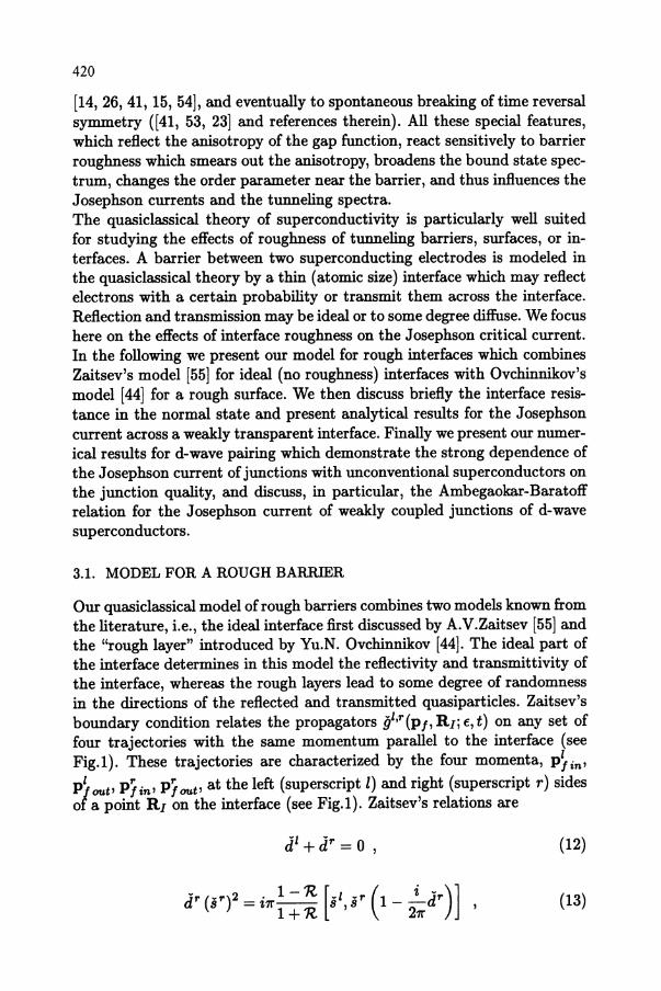
Our quasiclassical model of rough barriers combines two models known from the literature, Le., the ideal interface first discussed by A.V.Zaitsev [55] and the "rough layer" introduced by Yu.N. Ovchinnikov [44]. The ideal part of the interface determines in this model the reflectivity and transmittivity of the interface, whereas the rough layers lead to some degree of randomness in the directions of the reflected and transmitted quasiparticles. Zaitsev's boundary condition relates the propagators g"r(p" RJj €, t) on any set of four trajectories with the same momentum parallel to the interface (see Fig.1). These trajectories are characterized by the four momenta, P~in' P~ out' PI in' PI out' at the left (superscript l) and right (superscript r) sides of a point RJ on the interface (see Fig.1). Zaitsev's relations are

ti' + tir = 0 , (12)

(13)

421

5 I 5'

Figure 2. 8ketch of our interface model. The ideal interface (I) separates two different superconductors (8,8'), whose Fermi surfaces (curved lines) are shown on the right and left sides. Parallel momentum and energy are conserved in a transmission and reflection process which fixes, as shown, the four momenta, pj:n,out. The interface is coated by rough layers (dotted area).

where'R, = 'R,(P~in) = 'R,(P/in) is the reflection parameter, and dB, SB (8 = l, r) are defined as the difference and sum of propagators of quasiparticles on incoming trajectories before reflection (incoming velocity, momentum pj in) and on outgoing trajectories after reflection (outgoing velocity, momentum pjout),

dB(pjin' R]i €, t) =

S8(pjin' R]i €, t) gB(pjout,RIj€,t) - gB(pjin' RIj €,t) 9 8(Pj out, R]i €, t) + 9 B(pjin' RIj €, t)

(14) (15)

We follow here the notation of A.I. Larkin & Yu.N. Ovchinnikov [35] in­troduced in section 1, and use Nambu-Keldysh matrix propagators, indi­cated by a "hacek". Parallel momentum is conserved at an ideal interface, which fixes, together with energy conservation, the kinematics of interface scattering as shown in Fig.1. In the normal state a quasiparticle moving towards the point R] at the interface with a momentum pj in can ei­ther be reflected with probability 'R,(Pj in) or transmitted with probability 7(pj in) = 1 - 'R.(pj in) to the outgoing trajectory on the other side of the interface. Two more channels open in the superconducting state because

422

of Andreev scattering. An incoming quasiparticle can be "retroreflected" (velocity reversal) into its incoming trajectory or transmitted into the in­coming trajectory on the other side of the interface. The function 'R(pj in)

is considered here a phenomenological model describing the reflection and transmission properties of the ideal interface without roughness. We model the roughness of an interface by coating it on both sides by a thin layer of thickness 6 of a strongly disordered metal (see Fig.l). These "rough layers" are distinguished from the adjacent metals only by their very short mean free path t. Only the ratio 6/ t matters in the limit 6, t ---+ 0, and defines the roughness parameter P = 6/ t. We include regular elastic scattering as well as pair-breaking scattering (e.g., spin-flip scattering, in­elastic scattering), and introduce two roughness parameters, Po (regular scattering) and Pin (pair-breaking scattering). Vanishing p's correspond to a perfect interface, and P = 00 to a diffuse interface, i.e., a reflected or transmitted quasiparticle looses its memory of the incoming direction. In the quasiclassical equations for the rough layers all but the scattering terms can be dropped, and one obtains the following transport equation in the rough layer.

_ [Pin (_"r) + Po (-"r) -l,r] + .-l,ra -l,r - 0 2 93 ± 2 9 ±, 9 ~ V 1. ~9 - ,

7r 7r -(16)

where the superscripts l and r distinguish the metals on the left and right sides of the interface, 93 is the Nambu-Keldysh matrix obtained from 9 by keeping only the T3-components of its Nambu submatrices, x is the spatial coordinate perpendicular to the interface, measured in units of 6, and the dimensionless velocity v i:r is the perpendicular component of the quasiparticle velocity normalized by an averaged Fermi velocity, v l,r =

v t / J(lvtI2). The left and right rough layers are located between x = -1

and x = +1, and are separated by Zaitsev's ideal interface at x = 0 (see Fig.l). In general, the quasiclassical propagators in the rough layers depend on PI, R], €, t, and the spatial variable x which specifies the position in the infinitesimally thin rough layer. We use Ovchinnikov's model [44] for the scattering processes in the rough lay.ers. In this model scattering preserves the sign of v 1.; particles moving towards the interface are not scattered into outgoing directions and- vice versa. This "conservation of direction" is indicated in (16) by the indices ± in the scattering terms, which stand for averaging over the momenta corresponding to v 1. > ° and v 1. < 0, respectively. We assume equal scattering probability into all states compatible with Ovchinnikov's conservation of direction. A reversal of the velocity may only happen at Zaitsev's interface which separates the two rough layers. In order to obtain the current-phase relationship of the junction we solve the

423

quasiclassical transport equations in both superconductors and in the rough layers. The solution in the left superconductor has to match continuously the solution at x = -1 in the left rough layer and, equivalently, the solution in the right superconductor has to match the solution in the right rough layer at x = 1. At x = 0 the solutions in the rough layers are matched via Zaitsev's conditions (12, 13). The order parameter has to be determined self-consistently. To get a finite current we fix the phase difference of the order parameter across the junction,

(17)

where the phases 1jJ1 and 1jJr at the interface point RJ are determined by

(18)

-I lr Here, !::t. ,r (p i ) are convenient reference order parameters on the left and right sides. The reference order parameter can be taken real in the cases discussed in this paper. Note that the phase difference is measured directly at the interface at point RJ. The current density is obtained by standard formulas of the quasiclassical theory, i.e.,

'(R )_jd€j d2pI (AAK( R. )) J ,t - 411"i (211")31 vII eVltr 739 PI, ,€,t (19)

in the Keldysh formulation, and

in the Matsubara formulation. The critical Josephson current is obtained as the maximum supercurrent across the junction in equilibrium. The Fermi velocity, v I (p I), is a function of the momentum. This function has the sym­metry of the lattice, and will be understood here as a material parameter, to be taken from theoretical models or from experiment, if available. This completes our brief review of the quasiclassical equations for a rough interface.

3.2. NORMAL STATE RESISTANCE

In this section we calculate the normal state resistance of our model inter­face, and show that interface roughness does not affect the interface resis­tance. This is a unique feature of Ovchinnikov's model for a rough layer which is very convenient for studying the effects of interface roughness at fixed interface resistance.

424

In the normal state the retarded and advanced propagators gR and gA are trivial, and given by gR,A = =Fi1l"f3, and the Keldysh propagator can be parameterized in terms of a distribution function <t>(PJ' R; €, t),

~K( R' t) - 4 . ( <t>(PJ,R;€,t) 0 ) 9 PI, ,€, - 11"~ 0 <t>(-p R' -€ t) I, , ,

(21)

Given <t> one can calculate the current density from

(22)

The distribution function in the rough layers can be calculated by solving the Landau-Boltzmann transport equation,

(23)

which follows by taking the normal state limit of the general quasiclassical transport equation (16). In this normal state limit the scattering rates for elastic and inelastic scattering can be added up to a total scattering rate Ptot = Po + Pin' Zaitsev's boundary conditions (12, 13) at an ideal interface turn in the normal state into the following classical boundary conditions for the distribution function at the left and right sides of the boundary at x= 0,

<t>'(p~out) = R(P~in) <t>'(P~in) + T(P/in) <t>r(p/in) (24)

<t>r(p/out) R(P/in) <t>r(p/in) + T(P~in) <t>'(P~in) (25)

In addition, the solutions of (23) in the two rough layers have to be matched at x = ±1 to the physical distribution functions on the left and right sides of the interface. In order to calculate the interface resistance we apply a voltage V to our junction, solve the transport equation (23) subject to the proper matching conditions at x = 0 and x = ±1, and calculate the current from (22). We assume that the junction is formed by vefY good conductors separated by a weakly transparent interface, such that the total resistance of the junction is dominated by interface scattering, and the voltage drop is to a good approximation localized at the interface. This leads to a difference e V of the electrochemical potentials in the two conductors, which drives the current. It is assumed that both conductors are in thermal equilibrium far away from the interface. This fixes the incoming parts of the distribution function on the left and right sides of the rough interface,

425

where f is the Fermi function at temperature T. The outgoing excitations are not in equilibrium, and their distribution function must in general be calculated from the transport equation (23). This calculation can be skipped in Ovchinnikov's model. In this model the number of incoming and out­going excitations are conserved separately, and the incoming part of the equilibrium distribution function on the left (right) side ofthe interface are solutions of the transport equation (23) at x < 0 (x > 0). This pins down the total current in terms of the incoming parts of the thermal distribution functions far away from the interface. The distribution functions at x = -0 (x = +0) are given by the sum of the incoming equilibrium distribution function on the left (right) side, the reflected distribution function, and the transmitted distribution function from the other side. On the right side of the interface we have

cpr(p/in'x = +Oje) = f(e+eV) , (27)

cpr (p/aut, x = +OJ e) = 'R(P/in)f(e + eV) + T(P~in)f(e) , (28)

and the equivalent formulas hold on the left side. The current density is constant, and can be calculated at any convenient point of the junction. We pick x = +0, and obtain by inserting the distri­bution functions (27,28) into (22)

h ~ 2e fa.. (j(2~;~~ I vh['R.(p'i,.)f«+ eV) + T(p~,.)f(€)l

! d2p/ in r f( V)) + (211")3Iv/IV/-L e+e . (29)

We now use the relations 'R(P/in) = 1 - T(P/in), T(P~in) = T(P/in)' and

~pr ~pr I in r (r ) I aut r (r) (30)

7{2-1I"-:-)-=-3-:-I-v ...... ,{..,...P'-'-in-:-)"""7IV/-L P/in = - (211")31 v,{p,aut) IV/-L Plaut ,

and obtain

1 ! d2pr h = RNA V = (2e2 (211")31:; IV/-LT{P~in))V (31)

Equation (30) is a geometric relation which follows from conservation of parallel momentum. For clarity we write down in (30) explicitly the mo­mentum dependence of the velocity. The factor in brackets in (31) is the interface conductance per area, l/(RN A), where A is the area of the inter­face. The conductance is obviously independent of the scattering rate Ptot, i.e., independent of the roughness of the interface.

426

3.3. WEAKLY TRANSPARENT INTERFACE

Zaitsev's boundary conditions (12, 13) at x = 0 can be simplified sub­stantially for a weakly transparent interface (7 « 1). We expand the Matsubara propagator gM to first order in the transmission amplitude, 7: gM = gAA + gM + O(~). The solution gAA corresponds to the equilibrium solution of a non-transparent interface. Both sides are decoupled in this case, and Zaitsev's boundary conditions turn into dtci/ = dtci{ = O. Hence,

the Oth order propagators on the left and right sides of the interface de­scribe superconductors bounded by a rough, non-transparent surface. The first order correction to the difference of the incoming and reflected prop­agator, dtf) = gM(pjt,x = Oj€n) - gM(p}n,x = Oj€n), can be obtained

directly from (13) in terms of the Oth order propagators, i.e. without having to solve the quasiclassical transport equation for gM. Expansion of (13) to first order in the transparency 7 [6] leads to

d'Mr i 7[AMl AMr] (1) = - 811" 8(0)' 8(0) . (32)

Equation (30) implies that the current density (20) can be written in terms ot the difference, dM , of outgoing and incoming propagators alone, and does not depend on the sum. Hence, one can calculate from Eq. (32) the Josephson current in terms of the Oth order quantities 8tci)' and 8tcir The straight forward calculation leads to the following formula for the current­phase relation.

2 ! d2pr iJ(1/J,T) = :kBT~ (211")/1:~ I vj-L7 (P/)

x ([/tYo~ (p~j €n)ltYo) (P/j en) + l:to~(p~j €n)/:to) (P/j en)] sin( 1/J)

+[/tYo~ (p~j €n)/:to) (pjj en) - l:to~ (p~j €n)ltYo) (P/j en)] cos(1/J)) ,(33)

where If and If! are the off-diagonal components of the propagator 9M(Pf'x = Oj€n), defined via gM = Iff} + If!f2 + gMf3. In the case of real reference order parameters ~l,r (this is a possible choice for an s-wave or d-wave superconductor but, e.g., not for d+is) the term propor­tional cos( 1/J) vanishes, and we get the standard sinusoidal behavior of the Josephson current iJ [12]. We note that the Josephson current vanishes in the limit of strong inelastic roughness, Pin -+ 00. The reason is that the off-diagonal components of gM decay to zero in the dirty layer. Hence, one has gM = -i1l"8gn(€n)f3 at x = 0, and the current is zero.

427

3.4. CALCULATION OF THE JOSEPHSON CURRENT

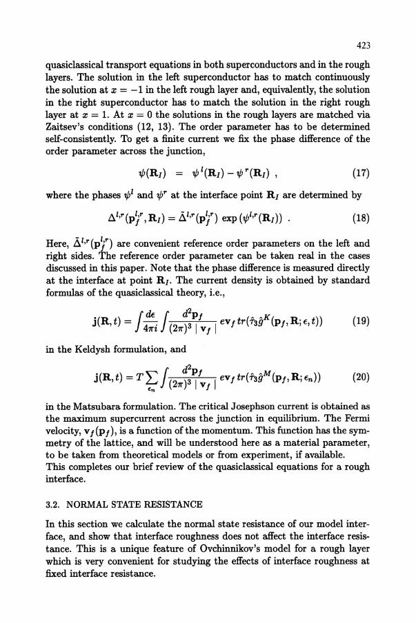
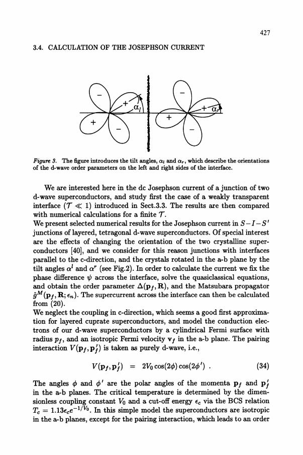
Figure 3. The figure introduces the tilt angles, al and a r , which describe the orientations of the d-wave order parameters on the left and right sides of the interface.

We are interested here in the dc Josephson current of a junction of two d-wave superconductors, and study first the case of a weakly transparent interface (7 « 1) introduced in Sect.3.3. The results are then compared with numerical calculations for a finite r. We present selected numerical results for the Josephson current in 8-1 -8' junctions of layered, tetragonal d-wave superconductors. Of special interest are the effects of changing the orientation of the two crystalline super­conductors [40J, and we consider for this reason junctions with interfaces parallel to the c-direction, and the crystals rotated in the a-b plane by the tilt angles 0 ' and or (see Fig.2). In order to calculate the current we fix the phase difference tP across the interface, solve the quasiclassical equations, and obtain the order parameter L\(P/' R), and the Matsubara propagator gM (PI' Rj en). The supercurrent across the interface can then be calculated from (20). We neglect the coupling in c-direction, which seems a good first approxima­tion for layered cuprate superconductors, and model the conduction elec­trons of our d-wave superconductors by a cylindrical Fermi surface with radius PI, and an isotropic Fermi velocity v I in the a-b plane. The pairing interaction V(PJ, PI) is taken as purely d-wave, i.e.,

V(PJ,p/) = 2Vocos(2¢)cos(2¢') (34)

The angles ¢ and ¢' are the polar angles of the momenta PI and p} in the a-b planes. The critical temperature is determined by the dimen­sionless coupling constant Vo and a cut-off energy €c via the BeS relation Tc = 1.13€ce-ljVo. In this simple model the superconductors are isotropic in the a-b planes, except for the pairing interaction, which leads to an order

428

M F=======~----~--l

'b .... .I0~ .. •. ..........•

....... .5"

~ 0.0 r.--~'~--:.::- -'-;--;=c--~--..;:.-;;=:- -:::;--=-~--~ ~ /' ,~~.- -

-ali< ; .' " E , , .. , !

-0.5 " ~ !/ CJ ! /

'. ' . <")

-1.0 '::'-'--'--::-::---::-:---::7--="=---:-' 0,0 0,4 0.6 0.6 ' .0

temperature TIT, 0.0 02 0,4 0.6 0.8 1.0

temperature TIT,

Figure 4. Temperature dependence of the Josephson critical current jc(T) of an ideal interface (Po = pin = 0) for different tilt angles 0/ = -o{ between 0° and 45°. (a) 'nInnel junctions (To = 0.01), (b) strongly coupled junctions (To = 0.50).

parameter, .6.{PJ) = .6. cos{24», with gap zeros and a sign change in (1,1) direction. Our interface is modeled by a reflection probability 'R.{O), and a roughness parameter PO. The pair-breaking scattering rate Pin is zero in this section. We follow [30] and choose the following one-parameter model for the de­pendence of 'R. on the angle of incidence 0,

'R.{ 0) _ 'R.o - 'R.o + (I - 'R.o) cos2(0)

(35)

It interpolates smoothly between a reflection probability 'R.o at perpendicu­lar incidence and total reflection ('R. = 1) at glancing incidence. All results presented in this section were obtained by numerical calculations, which involve a self-consistent calculation of the order parameter in. the supercon­ducting electrodes and of the scattering self-energy in the two rough layers.

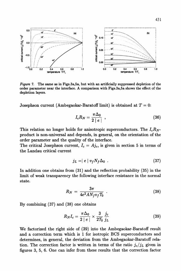
In Figs.3a,b we show the temperature dependence of the Josephson crit­ical current for d-wave superconductors, and ideally smooth (po = 0) inter­faces. We compare the cases of a very weak transparency (To = 1 -: 'R.o = 0.01) and a rather large transparency (To = 0.50). The critical currents are calculated for a representative set of tilt angles, 0:' = _o:r = 0°-45°. The critical current is normalized in all figures by iL = lelvJNJ.6.o which is the Landau critical current at T = 0 of a clean s-wave superconductor with the same Tc as the d-wave superconductor. Our results for d-wave supercon­ductors differ significantly from the Ambegaokar-Baratoff curve for s-wave superconductors. One finds [7]:

a) A strong dependence on the orientation of the crystals.

429

~ " "'---".-~/-/-/,-, '----'---:-:-:-:-::c-'-'-' -" ,-,,-, ,,-,, -,1

Z:- 0"0 k:-::--==~--~=~~ J i

0_04 '-(b-) ---_,--~--;:.--:-.-----,-~---.-~ . .. .. ... .. ... . ......... -~'-

". -........... . I

1- ~:l~: I' jl T-o __ •

,- - '-o~IT. ,--l~

=_----:-'"::-__ ~ __ J 0.5 1.0

phase .,Itc

-1.5 1'=-____ ~_:_=_---0.0 0.5

phase .,111:

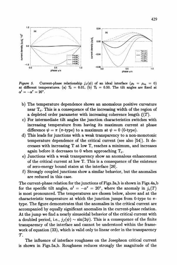
Figure 5. Current-phase relationship jJ(1j;) of an ideal interface (po = pin = 0) at different temperatures. (a) To = 0.01, (b) To = 0.50. The tilt angles are fixed at ol = -o{ = 20°.

b) The temperature dependence shows an anomalous positive curvature near Tc. This is a consequence of the increasing width of the region of a depleted order parameter with increasing coherence length ~(T).

c) For intermediate tilt angles the junction characteristics switches with increasing temperature from having its maximum current at phase difference t/J = 1r (1r-type) to a maximum at t/J = 0 (O-type).

d) This leads for junctions with a weak transparency to a non-monotonic temperature dependence of the critical current (see also [54]). It de­creases with increasing T at low T, reaches a minimum, and increases again before it decreases to 0 when approaching T c'

e) Junctions with a weak transparency show an anomalous enhancement of the critical current at low T. This is a consequence of the existence of zero-energy bound states at the interface [26].

f) Strongly coupled junctions show a similar behavior, but the anomalies are reduced in this case.

The current-phase relation for the junctions of Figs.3a,b is shown in Figs.4a,b for the specific tilt angles, ci = -at = 20°, where the anomaly in ic(T) is most pronounced. The temperatures are chosen below, above and at the characteristic temperature at which the junction jumps from Ootype to 1r­type. The figure demonstrates that the anomalies in the critical current are accompanied by equally significant anomalies in the current-phase relation. At the jump we find a nearly sinusoidal behavior of the critical current with a doubled period, Le., iJ(t/J) rv sin(2t/J). This is a consequence of the finite transparency of the interface and cannot be understood within the frame­work of equation (33), which is valid only to linear order in the transparency T.

The influence of interface roughness on the Josephson critical current is shown in Figs.5a,b. Roughness reduces strongly the magnitude of the

430

critical current of anisotropic superconductors, even at fixed normal state resistance. The reduction is in our cases by a factor 5 for (i = 0°, and by two orders of magnitude for a'~ 45°. The strong reduction of the Joseph­son current at diffuse interfaces can be understood in terms of a destruc­tive interference of contributions of different trajectories. This may occur if quasiparticles moving along different trajectories experience different phase changes of the order parameter when going from one side [d 8 (Pfin)] to the other side [d 8' (p f out)] ofthe junction. This effect requires anisotropic order parameters whose phase (e.g., the sign) changes with changing momentum direction. It is important to note that anomalies such as the transitions from a O-junction to a 1l"-junction, and the enhancement at low tempera­tures are sensitive to interface roughness, and have disappeared for Po = 2. At Po = 2 we have already reached to a good approximation the rough limit (po = 00) of our model. The results for Po > 2 are essentially unchanged compared to Po = 2, except for a l = _ar = 45° where iJ vanishes for Po = 00. Figs.6a,b finally demonstrate the role of the distorted order parameter near the interface. They show the calculated critical currents for a non­selfconsistent, constant order parameter. These approximate results exhibit the same qualitative features as Figs.3a,5a, but show significantly different magnitudes and T-dependences at temperatures above ~ 0.5 Te.

3.5. AMBEGAOKAR-BARATOFF RELATION

[2] derived a universal relation between the critical Josephson current across a junction of weakly coupled isotropic BCS superconductors, the energy gap and the junction resistance in the normal state (11). The maximum

ool j , I

I L--____ ~ __ J

0.0 0.2 0.4 0.6 0.8 1.0 temperature TIT.

I o·

0.0

~ 1 I I I

0.2 0.4 0.6 0.8 1.0 temperature TIT.

Figure 6. The same as in Figs.3a,b but for a rough interface (Po = 2, pin = 0).

431

O.5 F===== .....•. !If. .. ... .. .. _._ .•.. _"

,... IS". 'b F~"" "" " ~ :- 0.10 IS" •.•••• lUI I E' 0.0 ~I:--""""-':;':--:""----~=~ 'i ,'.,1 ,,/:z;,.

~ I ...... . • ..Jt r---JlI: --- - -----__ ....

~ ,,/0' "

I -0.5 :' ,;~ , .. , ,

/ ./ - 1.00.0 0.2 0.4 0 .6

temperllUre TIT,

i 005 r --~- . . . -..... """ ~ . _. _ _ li . ____ . __ ~_~:- - .. -.--:~. >->'" ! l! ---"-' -. . . I :6 0.00 --... .. -.-.~:::~:~'-:-

L ______________ ~ __ ~ 1.0 0.0 0.2 0.4 0 .6 0.8 1.0

tempefaJure TIT,

Figure 7. The same as in Figs.3a,5a, but with an artificially suppressed depletion of the order parameter near the interface. A comparison with Figs,3a,5a shows the effect of the depletion layers.

Josephson current (Ambegaokar-Baratoff limit) is obtained at T = 0:

1I'Ao IeRN=~ , (36)

This relation no longer holds for anisotropic superconductors. The IeRN­product is non-universal and depends, in general, on the orientation of the order parameter and the quality of the interface. The critical Josephson current, Ie = Aie, is given in section 5 in terms of the Landau critical current

(37)

In addition one obtains from (31) and the reflection probability (35) in the limit of weak transparency the following interface resistance in the normal state.

311' RN =

4e2ANfvfTo

By combining (37) and (38) one obtains

(38)

(39)

We factorized the right side of (39) into the Ambegaokar-Baratoff result and a correction term which is 1 for isotropic BCS superconductors and determines, in general, the deviation from the Ambegaokar-Baratoff rela­tion. The correction factor is written in terms of the ratio ie/ iL given in figures 3, 5, 6. One can infer from these results that the correction factor

432

1.0

0.00.0 0 .2 0 .4 0 .6 temperature TIT.

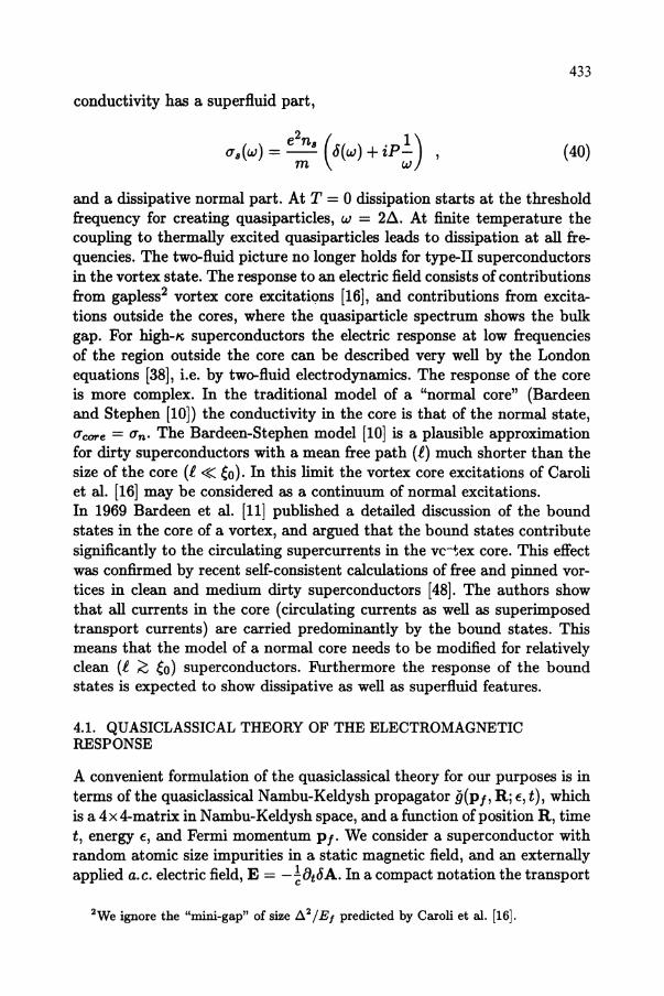
Figure 8. Temperature depen­dence of the critical current den­sity of a symmetric single grain boundary junction. The experimen­tal data are taken from Mannhart et al. (1988) (10° (D) and 15° (0) YBa2Cu307-6 tilt boundary). The solid (dashed) line is a theoretical curve obtained from our model for d-wave (s-wave) pairing with inter­face parameters To = 0.001, Po = 0.5, Pin = 0, ci = -at = 5° (To = 0.001, Po = 0, Pin = 0.34). Dotted line: Am­begaokar-Baratoff formula [Eq. (1)].

may be negative and larger than 1 for idealjunctions with d-wave supercon­ductors (see Fig.3a), and is much smaller than 1 for rough junctions with d-wave superconductors (see Fig.5a). In addition, the correction factor de­pends strongly on the orientation of the order parameter (see Figs.3, 5). In Fig.7 we compare temperature dependent critical current measurements on symmetric single grain boundary junctions by J. Mannhart et al. [40J (10° and 15° YBCO tilt boundaries) with our theoretical calculations. Our calculations have shown that the standard Fermi-liquid theory of supercon­ductivity in correlated, anisotropic metals predicts characteristic differences for d-wave and s-wave superconductors in the temperature dependence of the Josephson current and the current-phase relation. These differences are to some degree washed out by interface roughness, such that the best way to observe these effects would be experiments on ideally clean grain bound­ary junctions with a weak transparency, and the possibility of continuously varying the tilt angles.

4. Electromagnetic Response of a Pancake Vortex in Layered Superconductors

In oder to demonstrate the capacities of the Fermi liquid theory of super­conductivity we apply in this section the quasiclassical theory of supercon­ductivity to a non-trivial dynamical problem. We calculate the response of the currents in the core of a vortex to an alternating electric field. An electric field has two principal effects on a superconductor. It changes the supercurrents by accelerating the superfluid condensate, and it generates dissipation by exciting "normal" quasiparticles. This two-fluid picture of a condensate and normal excitations is clearly reflected in the optical conduc­tivity of standard s-wave superconductors in the Meissner state [42J. The

433

conductivity has a superfluid part,

0"8{W) = e:, (6{w) + iP~) , (40)

and a dissipative normal part. At T = 0 dissipation starts at the threshold frequency for creating quasiparticles, w = 2~. At finite temperature the coupling to thermally excited quasiparticles leads to dissipation at all fre­quencies. The two-fluid picture no longer holds for type-II superconductors in the vortex state. The response to an electric field consists of contributions from gapless2 vortex core excitations [16J, and contributions from excita­tions outside the cores, where the quasiparticle spectrum shows the bulk gap. For high-K superconductors the electric response at low frequencies of the region outside the core can be described very well by the London equations [38J, i.e. by two-fluid electrodynamics. The response of the core is more complex. In the traditional model of a "normal core" (Bardeen and Stephen [10]) the conductivity in the core is that of the normal state, O"core = O"n. The Bardeen-Stephen model [lOJ is a plausible approximation for dirty superconductors with a mean free path (l) much shorter than the size of the core (l « ~o). In this limit the vortex core excitations of Caroli et al. [16J may be considered as a continuum of normal excitations. In 1969 Bardeen et al. [l1J published a detailed discussion of the bound states in the core of a vortex, and argued that the bound states contribute significantly to the circulating supercurrents in the vc-~ex core. This effect was confirmed by recent self-consistent calculations of free and pinned vor­tices in clean and medium dirty superconductors [48J. The authors show that all currents in the core (circulating currents as well as superimposed transport currents) are carried predominantly by the bound states. This means that the model of a normal core needs to be modified for relatively clean (l ;G ~o) superconductors. Furthermore the response of the bound states is expected to show dissipative as well as superfluid features.

4.1. QUASICLASSICAL THEORY OF THE ELECTROMAGNETIC RESPONSE

A convenient formulation of the quasiclassical theory for our purposes is in terms of the quasiclassical Nambu-Keldysh propagator 9(Pf' Rj €, t), which is a 4 x 4-matrix in N ambu-Keldysh space, and a function of position R, time t, energy €, and Fermi momentum Pf' We consider a superconductor with random atomic size impurities in a static magnetic field, and an externally applied a.c. electric field, E = -~8tt5A. In a compact notation the transport

2We ignore the "mini-gap" of size 1:::.2 / Ef predicted by Caroli et aI. [16].

434

equation for this system and the normalization condition read

e ¥

[(€ + -vI· A)T3 - AmI - Ui - c5iJ ,g]® + iV/· Vg = 0 (41) c

g®g=-7r2i, (42)

where A(R) is the vector potential of the static magnetic field, B = V x A, Am/(P/, R; t) the mean-field order parameter matrix, and ui(P/, R; €, t) is the impurity self-energy. The perturbation c5iJ(P/, R; t) includes the external electric field and the field of the charge fluctuations, c5p(R; t), induced by the external field. For convenience we describe the external electric field by a vector potential c5A(R; t) and the induced electric field by the electro­chemical potential c5<p(R; t). Hence in the Nambu-Keldysh matrix notation the perturbation has the form,

e ¥

c5iJ = --v I . c5A(R; t)f3 + ec5<p(R; t)l , c

(43)

and is assumed to be sufficiently small so that it can be treated in linear response theory. Equations (41) and (42) must be supplemented by self-consistency equa­tions for the order parameter and the impurity self-energy. We use the weak-coupling gap equations,

(44)

(45)

and the impurity self-energy in Born approximation with isotropic scatter-ing,

(46)

where j K is the off-diagonal part of the 2 x 2 N ambu matrix gK, and the Fermi surface average is defined by

(47)

The materials parameters that enter the self-consistency equations are the pairing interaction, V (p I, PJ)' the impurity scattering lifetime, T, in addi­tion to the Fermi surface data PI (Fermi surface), v I (Fermi velocity), and

d2pt N, = J (21l-)3lv tl· In the linear response approximation one splits the propagator and the

435

self-energies into an unperturbed part and a term of first order in the per­turbation,

and expands the transport equation and normalization condition through first order. In oth order we obtain

e y

[(€ + -vJ· A)f3 - AmJO - 0-0 ,00J® + iVJ· VOo = 0 , c

Y 10\ Y 21Y

90 I(Y 90 = -7r ,

and in 1st order

(49)

(50)

e y Y

[(€+ -vJ· A)f3 - AmJo - 0-0 ,dO]® +ivJ· VdO = [dAmJ +do-i +dv, ooJ® , c

(51) 00 ® dO + dO ® 00 = 0 . (52)

In order to close this system of equations one has to supplement the trans­port and normalization equations with the self-consistency equations of oth and 1st order:

(53)

(54) and

1 o-o(R; €) = -2 (Oo(p/, R; E)) ,

7r'T (55)

1 do-i(R; €, t) = -2 (60(p/, R; €, t))

7r'T (56)

Finally, the electro-chemical potential, d<p, is determined by the condition of local charge neutrality [25, 5J. This condition follows from the expansion of charge density to leading order in the quasiclassical expansion parameters. One obtains dp(R; t) = 0, i.e.

The self-consistency equations (53)-(56) are of vital importance in the con­text of this paper. Equations (54) and (56) for the response of the quasiclas­sical self-energies are equivalent to vertex corrections in the Green's func­tion response theory. They guarantee that the quasiclassical theory does

436

not violate fundamental conservation laws. In particular, (55) and (56) im­ply charge conservation in scattering processes, whereas (53) and (54) imply charge conservation in a particle-hole conversion process. Any charge which is lost or gained in a particle-hole conversion process is balanced by the cor­responding gain or loss of condensate charge. It is the coupled quasiparticle dynamics and collective condensate dynamics which conserves charge in superconductors. Neglect of the dynamics of either component, or use of a non-conserving approximation for the coupling of quasiparticles and col­lective degrees of freedom leads to unphysical results. Condition (57) is a cl.JLsequence of the long-range of the Coulomb repulsion. The Coulomb energy of a charged region of size ~3 and typical charge density eN11:! is rv e2 NJ I:! 2 ~8, which should be compared with the condensation energy rv NI1:!2~3. Thus, the cost in Coulomb energy is a factor (EJlI:!)2 larger than the condensation energy. This leads to a strong suppression of charge fluctuations, and the condition of local charge neutrality holds to very good accuracy for superconducting phenomena. Equations (49)-(57) constitute a complete set of equations for calculating the electromagnetic response of a vortex. The structure of a vortex in equi­librium is obtained from (49), (50), (53) and (55), and the linear response of the vortex to the perturbation 6A(Rj t) follows from (51), (52), (54), (56) and (57). The currents induced by 6A(Rj t) can then be calculated directly from the Keldysh propagator 6gK via

4.2. STRUCTURE AND SPECTRUM OF A PANCAKE VORTEX

We consider an isolated pancake vortex in a strongly anisotropic, layered superconductor, and model the Fermi surface of these systems by a cylin­der of radius PI, and a Fermi velocity of constant magnitude, VI, along the layers. We also assume isotropic (s-wave) pairing and isotropic impurity scattering. Thus, the materials parameters of the model superconductor are: Tc , V I, the 2D density of states N I = PI / 27rV I, and the mean free path i = VIT. The model superconductor is type II with a large Ginzburg­Landau parameter /'i, ~ 100, so the magnetic field is to good approximation constant in the region of the vortex core. We first present results for the equilibrium vortex. The order parameter, l:!o(R), is calculated by solving the transport equation (49), the gap equa­tion (53), and the self-energy equation (55) self-consistently. These calcula­tions are done at Matsubara energies (€ --+ i€n = i(2n+1)7rT). Details of the numerical schemes for solving the transport equation self-consistently are

437

1.5

.... " -"" 1.0 -~ ~ 0.2

0.5

aj

0.0 '-'--~--'--'~~..........l~~-,-,-~~.......J 0·~/'-0.0~~....J_5'-.0~~...l0.0~"":""'~5-'-.0~~.......JIO.O

R / v/2.T, -10.0 -5.0 0.0 5.0 10.0

R / v/2.T,

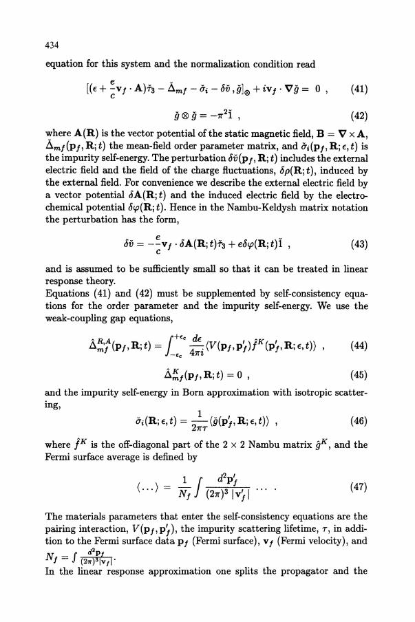
Figure g. Results of self-consistent calculations of the modulus of order parameter (a) and the current density (b) at T = O.3Te for superconductors with electron mean free path l = Weo (clean) to l = ~eo (dirty). R is the distance from the vortex center measured in units of the coherence length.

given elsewhere [22]. Charge conservation for the equilibrium vortex follows from the circular symmetry of the currents. Nevertheless, self-consistency of the equilibrium vortex is important; the equilibrium self-energies (Llo, 0"0) and propagators (go) are input quantities in the transport equation (51) for the linear response. Charge conservation in linear response is non­trivial and requires self-consistency of both the equilibrium solution and the solution in first order in the perturbation.

Fig.1 shows the order parameter and the current density in the vortex core of an equilibrium vortex for different impurity scattering rates 'T. As expected, scattering reduces the coherence length and thus the size of the core, and has a strong effect on the current density. Numerical results for the excitation spectrum of bound and continuum states at the vortex together with the corresponding spectral current densities are shown in Fig.2. The local density of states (per spin) and the spectral current density are defined by

N(R,€)

j(R,€)

Nf 4~ Tr(T3 (gR(Pf, R, €) - gA(Pf, R, €)) ) (59)

eNf 2~ Tr(T3 V f(Pf) (gR(pj, R, €) - gA(pj, R, €))) . (60)

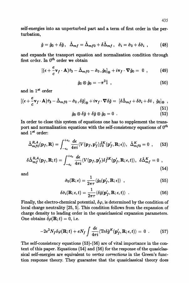
The zero-energy bound state is remarkably broadened by impurity scatter­ing. Its width is well approximated by the scattering rate 1/(vfl), which is G.63Tc for l = 10{0. The broadening of the bound states decreases with increasing energy. The results for the spectral current density (Fig.2b) show that nearly all of the current density of the equilibrium vortex resides in the energy range of the bound states. This reflects the observation that the supercurrents in the vortex core are predominantly carried by the bound

438

3. a r"'""" ............................. r-r ............................. r-r ................... ...,...,..., b)

3.0 2.0

",,' ,:--~""

~..., .. ~ 2.0 .... 1.0 ~ -... ~ ~

~ ~

1.0 0.0

0.0 1.0 2.0 3.0

Figure 10. Local density of states N(R, E) (a) and local spectral current density j.., (R, E) (b) in the vortex core of a superconductor with l = lO~o at T = 0.3Tc. Results are shown for a series of spatial points on the y-axis, at distances 0, .2511'~O, .511'~O, ... ,411'~O from the vortex center. The thickest full line corresponds to the vortex center, and decreasing thickness indicates increasing distance from the center. Results for the outermost point (411'~o) are shown as dashed lines. The thin dotted lines show the density of states of the homogeneous superconductor (a) and the value of the bulk gap (b) respectively.

states [11, 48]. The physics of the core is dominated by the bound states, in particular also, as we will show, the response of the core to an electric field.

4.3. DISTRlBUTION FUNCTIONS

The set of formulas for calculating the quasiclassical linear response of a superconductor is given in a compact notation in (48)-(57). In this sec­tion we transform these formulas into a more suitable form for analytical and numerical calculations. The central differential equation of the qua­siclassical response theory is the transport equation (51). It comprises 12 differential equations for the components of the three 2 x 2-N ambu matrices, dgR,A,K. The number of differential equations can be reduced significantly by using general symmetry relations and the normalization conditions of the quasiclassical theory. We focus on the simplifications which follow from the normalization equations (50) and (52). We use the projection operators

439

introduced by Shelankov [51J,

PR,A = ~ (i + _1_ AR,A) P!!,A = ~ (i _ ~9AOR'A) . + 2 _i7r 90 ' 2 -Z7r

(61)

ARA ARA A Obviously, P +' + p _ ' = 1. The algebra of the projection operators follows from the normalization conditions.

(P!,A)2 = P!,A, (P!!,A)2 = P!!,A,

P!,A P!!,A = P!!,A P!,A = o. (62)

A key result is that the Nambu matrices &gR,A,K can be expressed, with the help of Shelankov's projectors, in terms of 6 scalar distribution /unctions, &,R,A, &i'R,A, &xa and &xa, each of which is a function of PI, R, €, t, and satisfies a scalar transport equation. The distribution functions are defined by

and

&ga (64)

= _ 27ri [P! ® (&~a ~) ® p~ + p~ ® (~ &~a) ® Pt]

where the anomalous response, &ga, is defined in terms of &gK, &gR,&gA by

&gK = &gR ® tanh(,8€/2) _ tanh(,8€/2) ® &gA + &ga , (65)

The transport equations for the various distribution functions follow from (49) and (51) and one finds [22],

iv I . V &,R,A + 2€&,R,A + (T:,A tiR,A _ ~R,A) ® &,R,A + &,R,A ® (tiR,A,:,A + ~R,A) (66)

= _,:,A ® &ti R,A ® ,:,A + &~R,A ® ,:,A _ ,:,A ® &~R,A _ &Ll R,A,

iv I . V &i'R,A - 2€&i'R,A + (i':,A LlR,A _ ~R,A) ® &i'R,A + &i'R,A ® (LlR,Ai':,A + ~R,A) (67)

= -i':,A ® &LlR,A ® i':,A+ 6~R,A ® i'~,A _ i'~,A ® &~R,A_ &tiR,A,

440

iv I . Vaxa + i8taxa+ ('Yf ~ R_ ~R) ® axa + axa ® (t!. AiA + ~A) = 'Yf ® at,a ® it - at!.a ® it - 'Yf ® a~a - a~a , (68)

iv/· Vaxa - iBtaxa+ (if!l.R- t,R) ® axa + axa ® (/::..A'Yt + t,A) = if} ® a~a ® 'Yt - a/::..a ® 'Yt - if} ® ot!.a - at,a . (69)

We have used the following short-hand notation for the driving terms in the transport equations, which includes external potentials, perturbations and self-energies:

e ~ ~ ~R,A (~R'A t!.R'A) -~v/' AT3 + t!.m/O + O'iO = _~R,A t,R,A ,

ah = a/::..m / + M'i + ov , ahK = ahR ® tanh(,8€/2) - tanh(,8€/2) ® ohA + oha ,

(70)

(71)

(72)

(73)

The functions 'Y:,A and i:,A in (66)-(69) are defined by the following con­venient parameterization of the equilibriun.. propagators.

~R,A . 1 ( 1 - 'Y:,Ai:,A 2'Y:,A ) 90 = =fl7l'1 + R,A-R,A 2;yR,A (1 R,A-R,A) .

~ ~ 10 - -~ ~ (74)

After elimination of the time-dependence in (66)-(69) by Fourier transform one is left with four sets of ordinary differential equations along straight trajectories in R-space. For given right-hand sides these equations are de­coupled, and determine the distribution functions a'YR,A, oiR,A, oxa and oxa . On the other hand, the self-consistency conditions relate the right-hand sides of (66)-(69) to the solutions of (66)-(69). Hence, equations (66)-(69) may be considered either as a large system of linear differential equations of size six times the chosen number of trajectories, or as a self-consistency problem. We solved the self-consistency problem numerically using spe­cial algorithms for updating the right hand sides. Details of our numerical schemes for a self-consistent determination of the response functions are given elsewhere [22].

4.4. RESPONSE TO AN A.C. ELECTRIC FIELD

We consider a pancake vortex in a layered s-wave superconductor and cal­culate the response of the electric current density, oj (R; t), to a small homo­geneous a.c. electric field, oEW(t) = oE exp( -iwt). The results presented in

_ .. _-- .. _ .. _-­--- .. ---~ ..... ---------------

441

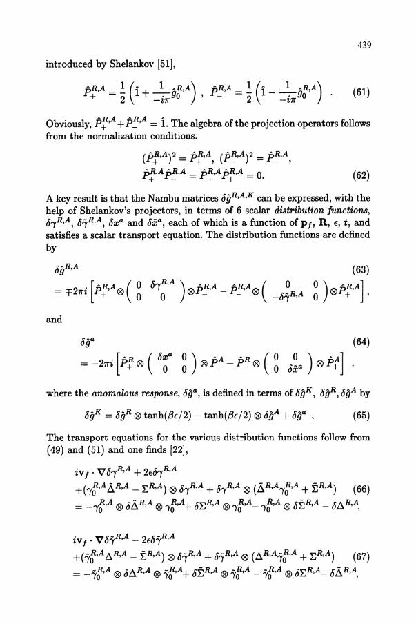
Figure 11. Snapshots of the time-dependent current pattern in the core of a pancake vortex at successive times, t = 0, -l2/, 12/, 12/, 12/, -&1 (upper left pattern to lower right pattern) . The arrows show the current density induced by an a.c. electric field in x-direction, E.,(t) = 5Ecos(wt), of frequency w = 21r/1 = 1.5A. The data are calculated in linear response approximation for a clean superconductor (l = WeD) at T = 0.3Tc. Current patterns in the second half-period, t = l I - H I, are obtained from the patterns in the first half-period by reversing the directions of the currents. The distance between two neighboring points on the hexagonal grid is 0.251reo.

this section are obtained by solving numerically the quasiclassical transport equations (66)-(69) together with the self-consistency equations (54), (56), and the condition oflocal charge neutrality (57). The calculation gives the local conductivity tensor, O"ij (R, w), defined' by

(75)

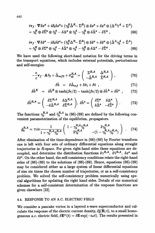
Figures 11 and 12 show the time development of the current pattern induced by an oscillating electric field in x-direction with time dependence tSEa:(t) = tSE cos(wt). Results are given for a medium range frequency (w = 1.5d) and a low frequency (w = O.3d). Two features should be emphMized. At medium and higher frequencies the current flow induced by the electric field is to good approximation uniform in space and phase shifted by 7r /2 (non-dissipative currents). The phase shift of 7r/2 is the consequence of a predominantly imaginary conductivity at frequencies above d, as shown in Fig.5. The current pattern at low frequencies (FigA) is qualitatively different. At the vortex center the current is phase shifted by ~ 7r / 4 in accordance with the conductivity at w = O.3d, which has about equal real ( dissipative) and imaginary (non-dissipative) parts, whereas further away

442

~ .......... '9 ~ " ................ " " ..

....... .A .... " to .. " , , ., t ,. .... ,. ...... ..

.... , , .. ,. .. ,. ........ .. ....... 'I' , ................ ...

.................. -_ ...... _---.................... ------ .. ---...................... ----- ... - .. ---. ............... IF.... ___________ _

.~................ ----- ... _----. ... " ... "",.... -----~.-~-----.......... \ .... I ... ., ...... .. . ... ~" .. ,,~...... ------, .. ,------

~ ........ ............. ."" ........... .. .-----,~~--- .. -. ------~~~------...... ----_ ......•..• _-------- .... ---------........ "."" ......... ... -.. --/~,--- ... ------~~~------....... , ... "........ --- .. ",."~--.. ------, .. ,------.... " ..... "..... .. .... "" .... ,"'..... -----_ ..... _-----...... , .......... ,',. . ..... .,............ ------- ... _----

", ....... "..... .................... ----_ .... _----................ ,. .... " .................. to... __________ _

.................. ,. .................... ----------.... ............... .............. ---------

--------------- --------------- ... ~~.-.,.~.~~. ---------------- ------ ••••• ----- •••• ~. ~~-,y~ •••• ______________________ ........ _____ •••••. 4 ___ 4 •••••

---------------- -----_ .... ------ ... ~~, ,-~~.~ ... . --------------- ---------#----- .. ~.,.,.-.~~ .. . -------------- -------------- ... ~~"-_, .... . ----._------- -------._---- ........ '---" .. .

Figure 12. The same as in fig. 11, but for a smaller external frequency, w = O.3~. The length of the current vectors is scaled down by a factor 5 compared to those in fig. 11.

from the center the conductivity becomes more and more non.dissipative. Fig.4 shows that the current flow at low frequencies is non-uniform. The dissipative currents exhibit a dipolar structure with enhanced currents at the vortex center, and back· flow currents away from the center. On the other hand, non· dissipative currents are approximately uniform.

The frequency dependence of the local conductivity, (7zz(R,w), for R along the x· and y·axis is shown in figures 13a,b. These figures include, for comparison, the Drude conductivity of the normal state and the con­ductivity of the homogeneous bulk superconductor. A significant feature of conductivity in the core is the strong increase of Re (7 at low frequencies. The conductivity is in this frequency range much larger than the normal state Drude conductivity and the exponentially small conductivity of the bulk s·wave superconductor. The real part of conductivity scales at low frequencies like l/w2• Its value at at the vortex center is 69.5e2N f vJ/Ll (outside the range of the figure) for w = a.ILl. The enhancement of the dis­sipative part at low frequencies is a consequence of the coupling of quasi­particles and collective order parameter modes, and cannot be obtained from non-selfconsistent calculations. Fig.13b shows that the real part of the conductivity becomes negative in the region of dipolar backfiow on the y-axis. This leads locally to a negative time averaged power absorption, < j . E >t < a, and a corresponding gain in energy, which is compensated by the strongly enhanced dissipation of energy in the center of the vortex. The dissipative part of the local conductivity at a distance R from the

aJ

------1.0 2.0 3.0

c.o/~

1.0

0.8

~;."" 0.6

~..., ~.,

'" ,-0.4

S ~ ~ ~ 0.2

0.0

-0.2 0.0 1.0 2.0

c.o/~

443

3.0

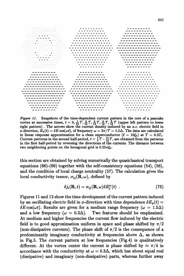
Figure 19. Frequency dependence of the real part ('lower' curves) and imaginary part ('upper' curves) of the local conductivity u.,., for a superconductor with parameters T = O.3Tc , l = toeo. For convenience, the conductivities are multiplied by w. The full black curves give the conductivity at the vortex center, and the series of dashed lines with decreasing intensity the conductivity at increasing distance from the center. Fig.13a presents data at points along the x-axis (in steps of (lI,/4)eo) , and Fig.13b at points along the y-axis (in steps of (V311'/4)eo). The dashed grey lines show the normal state Drude conductivity, and the full grey lines the conductivity of the homogeneous superconductor.

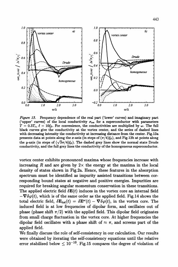
vortex center exhibits pronounced maxima whose frequencies increase with increasing R and are given by 2 x the energy at the maxima in the local density of states shown in Fig.2a. Hence, these features in the absorption spectrum must be identified as impurity assisted transitions between cor­responding bound states at negative and positive energies. Impurities are required for breaking angular momentum conservation in these transitions. The applied electric field oE(t} induces in the vortex core an internal field -VOI,O(t}, which is of the same order as the applied field. Fig.I4 shows the total electric field, oEtot(t} = oEW(t} - VOI,O(t}, in the vortex core. The induced field is at low frequencies of dipolar form, and oscillates out of phase (phase shift 71' /2) with the applied field. This dipolar field originates from small charge fluctuation in the vortex core. At higher frequencies the dipolar field oscillates with a phase shift of ~ 71', and screens part of the applied field. We finally discuss the role of self-consistency in our calculation. Our results were obtained by iterating the self-consistency equations until the relative error stabilized below::; 10-1°. Fig.I5 compares the degree of violation of

444

----------- ----------- - .. ---- .... ------------ ------------ .. _---------------------- ------------- .,.,-----_ .. . -------------- -------------- ... ,,~--"' .. . --------------- --------------- .... ,,~,,~ .. . ---------------- ---------------- ..... ,~~~ ... . ----------------- ----------------- ....... ---...... . ---------------- ---------------- ..... "---~ ..... . --------------- --------------- .... ,'~, .... . -------------- -------------- ... "'--~, ... . ------------- ------------- .-._------, .. ------------ ------------ .. -------_ .. ----------- ----------- .. _-.----.-.. .. .. .. .. .. .. .. .. .. .. .. .. .. .. .. .. .. ---------................ .. " .. . .. .. .. .. .. .. .. .. ----------

.... f ............ " , .. .. .. .. .. .. .. .. • •• __________ _ ............ " " l' l' ....... ".. ............... _____ .... ____ _ ~ •• 41 .. ' .... ".1'1'1' .............. ~. ........... _____ ..... _____ _

••••• , __ ••••• 0 ____ •••• ,..... _____________ _

.. .... ~~ ,~-". .... ...--,,"."~-........ -----" .. ,~-----· ........ ~/~\· ... · ... ·· ...... ---,~--,~-- ... - ... ------'.'-------......... __ . .. . .. .. ... ... ...... - -_ .... _ .... --_ ........ ------_ .... -------........ • \ ___ 1 ~ .. .. .. .... ... ...... __ .. , ......... ~ ....... _...... ... ______ ~ l' • , _____ _ ........ , It ,-~, ~ ~ l' .. .. ... ..... - ~ I IIj • , , ,_... ...... _____ ~, .. , ..... ____ _ ...... --,..... . .. "'" .. _--- --------------, , l' .. " ... , .... ~ • . .. , .. . ~ .. , .........

.. l' t " '" .......... . l' t " ............... .

.. " '" ............ . " '" ............ ..

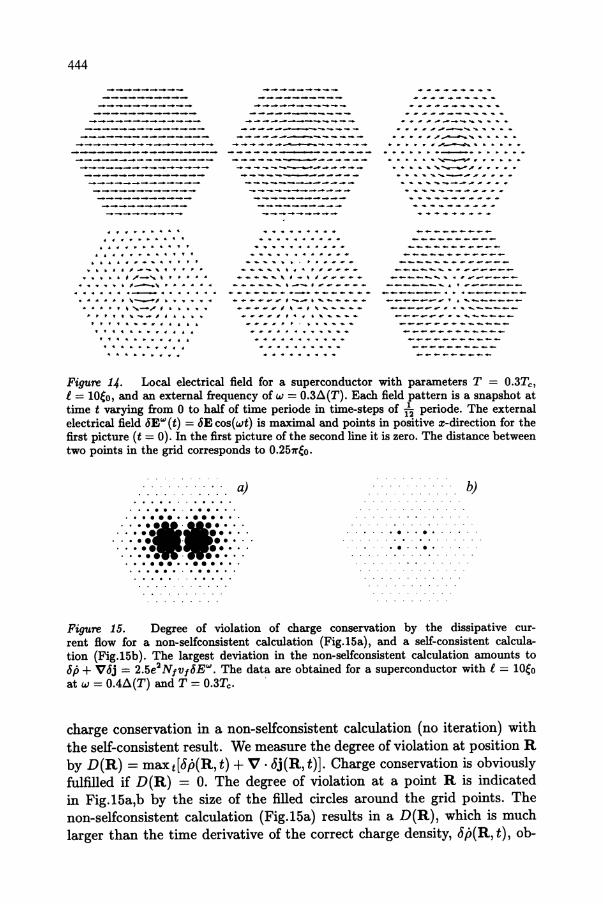
Figure 14. Local electrical field for a superconductor with parameters T = O.3Te, l = lOeo, and an external frequency of w = O.3A(T). Each field pattern is a snapshot at time t varying from 0 to half of time periode in time-steps of 12 periode. The external electrical field cSE'" (t) = cSE cos( wt) is maximal and points in positive x-direction for the first picture (t = 0). In the first picture of the second line it is zero. The distance between two points in the grid corresponds to O.251reo.

. . . . a) b)

. . . . .. . .... . . . . . .. . .. .. . . .. .

. -: ':-:-;-.·1-;-:-:-:-· . . . .. . ... . . . . .. . .... . ... ... . .....

. . . . .. .. .. .. . . . .

Figure 15. Degree of violation of charge conservation by the dissipative cur­rent flow for a non-selfconsistent calculation (Fig.15a), and a self-consistent calcula­tion (Fig.15b). The largest deviation in the non-selfconsistent calculation amounts to cSp + VcSj = 2.5e2 N,v,cSE"' . The data are obtained for a superconductor with l = lOeo at w = O.4A(T) and T = O.3Te.

charge conservation in a non-self consistent calculation (no iteration) with the self-consistent result. We measure the degree of violation at position R by D(R) = maxt[~p(R, t) + V . ~j(R, t)]. Charge conservation is obviously fulfilled if D(R) = O. The degree of violation at a point R is indicated in Fig.15a,b by the size of the filled circles around the grid points. The non-selfconsistent calculation (Fig.15a) results in a D(R), which is much larger than the time derivative of the correct charge density, ~p(R, t), ob-

445

tained from a self-consistent calculation with ~ip(R, t) = 0 instead of charge neutrality condition. In Fig.15b we show the violation of charge conserva­tion for our self-consistent calculation. The small remaining D(R) is here a consequence of the finite grid size used in our calculations.

4.5. DISCUSSION

In this section we used the quasiclassical theory to calculate the electro­magnetic response of a pancake vortex in a superconductor with finite but long mean free path. This complements previous calculations for perfectly clean systems, which were done self-consistently in the limit w -+ 0 [27J, and at finite frequencies without a self-consistent determination of the order parameter [28, 56]). The frequency range of interest in our calculations is of the order of the gap frequency, hw = a. We have shown that at low fre­quencies (nw < O.5a) the electromagnetic dissipation is strongly enhanced in the vortex cores above its normal state value, and that this effect is a con­sequence of the coupled dynamics of low-energy quasiparticles excitations bound to the vortex core and collective order parameter modes. The in­duced current density has at low frequencies a dipole-like behaviour, which results from an oscillating motion of the vortex perpendicular to direction of the driving a. c. field. The response of the vortex in the intermediate fre­quency range, .5a ;:s 1iw ;:s 2a, is dominated by bound states in the vortex core. We find peaks in the local dissipation at twice the bound state ener­gies. At higher frequencies, 1iw > 2a, the conductivity approaches that of a very clean homogeneous superconductor, which is in good approximation given by the non-dissipative response of an ideal conductor.

References

1. Ambegaokar, V. and Tewordt, L. (1964), Phys. Rev. 134, A805. 2. Ambegaokar, V. and Baratoff, A. (1963), Phys. Rev. Lett. 10, 486; 11, 104. 3. Ambegaokar, V., de Gennes, P.G. and Rainer, D. (1974), Phys. Rev. A 9, 2676. 4. Andreev, A.F. (1964), Sov. Phys. JETP 19, 1228. 5. Artemenko, S.N. and Volkov, A.F. (1979), Sov. Phys.-Usp. 22, 295. 6. Ashauer, B., Kieselmann, G. and Rainer, D. (1986), J. Low Temp. Phys. 36, 349. 7. Barash, Yu.S., Burkhardt, H. and Rainer D. (1996), Phys. Rev. Lett. 77, 4070. 8. Bardeen, J.; Cooper, L.N. and Schrieffer, J.R. (1957), Phys. Rev. 108, 1175. 9. Bardeen, J., Rickayzen, G. and Tewordt, L. (1995), Phys. Rev. 113, 982. 10. Bardeen, J. and Stephen, M.J. (1965), Phys. Rev. 140 A, 1197. 11. Bardeen, J., Kiimmel, R., Jacobs, A.E. and Tewordt, L., (1969), Phys. Rev. 187,

556. 12. Barone, A. and Paterno, G. (1982), Physics and Applications of the Josephson Effect

(Wiley & Sons, N.Y.). 13. Betbeder-Matibet, O. and Nozieres, P. (1969), Ann. Phys. 51, 329. 14. Buchholtz, L.J. and Zwicknagl, G. (1981), Phys.Rev. B 23, 5788. 15. Buchholtz, L.J., Palumbo M., Rainer, D. and Sauls, J.A. (1995),

J. Low Temp. Phys. 101, 1079.

446

16. Caroli, C., de Gennes, P.G., Matricon, J. (1964), Phys. Lett. 9,307. 17. de Gennes, P.G. (1966) Superconductivity in Metals and Alloys, .

W.A. Benjamin, New York; reprinted by Addison-Wesley, Reading, MA (1989). 18. Eckern, U. (1981), Ann. Phys. 133,390. 19. Eilenberger, G. (1968), Z. Physik 214, 195. 20. Eliashberg, G. (1962), Sov.Phys.-JETP 15, 1151. 21. Eliashberg, G.M. (1972), SOy. Phys. JETP 34, 668. 22. Eschrig, M. (1997), Ph.D. thesis, Bayreuth University. 23. Fogelstrom, M., Rainer, D. and Sauls, J.A. (1997), Phys. Rev. Lett. 19, 281. 24. Geilikman, B.T. (1958), SOy. Phys. JETP 1, 721 25. Gorkov, L.P. and Kopnin, N.B. (1975), SOy. Phys.-Usp. 18,496. 26. Hu, C.R. (1994), Phys. Rev. Lett. 12, 1526. 27. Hsu, T.C. (1993), Physica C 213, 305. 28. Janko, Boldizsar and Shore, J.D. (1992), Phys. Rev. B 46, 9270. 29. Keldysh, L.V. (1965), SOy. Phys. JETP 20, 1018. 30. Kieselmann, G. (1987), Phys. Rev. B 35, 6762. 31. Landau, L.D. (1957), SOy. Phys. JETP 3, 920.

Landau, L.D. (1957), SOy. Phys. JETP 5,101. Landau, L.D. (1959), SOy. Phys. JETP 8, 70.

32. Larkin, A.I. and Ovchinnikov, Yu.N. (1968), SOy. Phys.-JETP 26, 1200. 33. Larkin, A.I. and Ovchinnikov, Y.N. (1976), SOy. Phys. JETP 41, 960. 34. Larkin, A.I. and Ovchinnikov, Yu.N. (1977), SOy. Phys. JETP 46, 155. 35. Larkin, A.I. and Ovchinnikov, Yu.N. (1986), in Nonequilibrium Superconductivity,

edited by D. N. Langenberg and A. I. Larkin (Elsevier Science Publishers), 493. 36. Larkin, A.I. and Ovchinnikov, Yu.N. (1976), SOy. Phys. JETP 41, 960. 37. Leggett, A.J. (1965), Phys. Rev. Lett. 14, 536.

Leggett, A.J. (1965), Phys. Rev. 140, 1869. Leggett, A.J. (1966), Phys. Rev. 141, 119.

38. London, F. (1950), Superfluids, Vol.1; Wiley, New York. 39. Liiders, G. and Usadel, K.D. (1971), The Method of the Correlation Function

in Superconductivity Theory, Springer Tracts in Modern Physics No.56 (Springer, Berlin, 1971).

40. Mannhart, J., Chaudhari, P., Dimos, D., Tsuei, C.C. and McGuire, 'f.R. (1988), Phys. Rev. Lett. 61, 2476.

41. Matsumoto, M. and Shiba, H. (1995), J. Phys. Soc. Jpn. 64,3384. 42. Mattis, D.C. and Bardeen, J. (1958), Phys. Rev. 111, 412. 43. Migdal, A.B. (1958), SOy. Phys. JETP 1, 996. 44. Ovchinnikov, Yu.N. (1969), SOy. Phys. JETP 29, 853. 45. Parks, R.D. (ed.) (1969) Superconductivity 1+11, Marcel Dekker, New York. 46. Rainer D., in Recent Progress in Many-Body Theories, Vol.1

(Plenum Press New York 1988), 217. 47. Rainer, D. and Sauls, J. A. (1995), in Superconductivity, From Basic Physics to

the Latest Developments, Lecture Notes of the Spring College in Condensed Matter Physics, I.C.T.P., Trieste, ed. by P.N. Butcher and L. Yu, World Sci., Singapore.

48. Rainer, D., Sauls, J.A. and Waxman, D. (1996), Phys. Rev. B 54, 10094. 49. Schmid, A. and Schon, G. (1975), J. Low Temp. Phys. 20, 207. 50. Serene, J.W. and Rainer, D. (1983), Phys. Reports 101, 221. 51. Shelankov, A.L. (1984), SOy. Phys.-Solid State 26, 981. 52. Shelankov, A.L. (1985), J. Low Temp. Phys 60, 29. 53. Sigrist, M., Bailey, D.B. and Laughlin, R.B. (1995), Phys. Rev. Lett. 14, 3249. 54. Tanaka, Y. and Kashiwaya, S. (1996), Phys. Rev. 53, 9371. 55. Zaitsev, A.V. (1984), SOy. Phys. JETP 59, 1015. 56. Zhu, Yu-Dong, Zhang, Fu-Chun and Drew, H.D. (1993), Phys. Rev. B 41, 58.