Fermi acceleration in the randomized driven Lorentz gas and the Fermi-Ulam model

Fermi acceleration in the randomized driven Lorentz gas and the Fermi-Ulam model

A. K. Karlis,* P. K. Papachristou, and F. K. Diakonos†

Department of Physics, University of Athens, GR-15771 Athens, Greece

V. ConstantoudisInstitute of Microelectronics, NCSR Demokritos, P.O. Box 60228, Attiki, Greece

P. SchmelcherPhysikalisches Institut, Universität Heidelberg, Philosophenweg 12, 69120 Heidelberg, Germany

and Theoretische Chemie, Im Neuenheimer Feld 229, Universität Heidelberg, 69120 Heidelberg, Germany�Received 13 March 2007; revised manuscript received 15 June 2007; published 23 July 2007�

Fermi acceleration of an ensemble of noninteracting particles evolving in a stochastic two-moving wallvariant of the Fermi-Ulam model �FUM� and the phase randomized harmonically driven periodic Lorentz gasis investigated. As shown in �A. K. Karlis, P. K. Papachristou, F. K. Diakonos, V. Constantoudis, and P.Schmelcher, Phys. Rev. Lett. 97, 194102 �2006��, the static wall approximation, which ignores scattererdisplacement upon collision, leads to a substantial underestimation of the mean energy gain per collision. Inthis paper, we clarify the mechanism leading to the increased acceleration. Furthermore, the recently intro-duced hopping wall approximation is generalized for application in the randomized driven Lorentz gas. Uti-lizing the hopping approximation the asymptotic probability distribution function of the particle velocity isderived. Moreover, it is shown that, for harmonic driving, scatterer displacement upon collision increases theacceleration in both the driven Lorentz gas and the FUM by the same amount. On the other hand, theinvestigation of a randomized FUM, comprising one fixed and one moving wall driven by a sawtooth forcefunction, reveals that the presence of a particular asymmetry of the driving function leads to an increase ofacceleration that is different from that gained when symmetrical force functions are considered, for all finitenumber of collisions. This fact helps open up the prospect of designing accelerator devices by combiningdriving laws with specific symmetries to acquire a desired acceleration behavior for the ensemble of particles.

DOI: 10.1103/PhysRevE.76.016214 PACS number�s�: 05.45.Ac, 05.45.Pq

I. INTRODUCTION

In 1949 Fermi �1� proposed an acceleration mechanism ofcosmic ray particles interacting with a time dependent mag-netic field �for a review, see �2��. Ever since, this has been asubject of intense study in a broad range of systems in vari-ous areas of physics, including astrophysics �3–5�, plasmaphysics �6,7�, atom optics �8,9�, and has even been used forthe interpretation of experimental results in atomic physics�10�. Furthermore, when the mechanism is linked to higherdimensional time-dependent billiards, such as a time-dependent variant of the classic Lorentz Gas �11�, it has pro-found implications on statistical, molecular, and solid statephysics �12�.

Several modifications of the original model have beensuggested, one of which is the well-known Fermi-Ulammodel �FUM� �13–15� which describes the bouncing of aball between an oscillating and a fixed wall. FUM and itsvariants �16,17� have been the subject of extensive theoreti-cal �see Ref. �14� and references therein� and experimental�18–20� studies as they are simple to conceive but hard tounderstand in that their behavior is quite intricate.

The recurrence equations defining the dynamics of adriven billiard are, in general, of implicit form, which hin-

ders analytical treatment and complicates numerical simula-tions. For these reasons, a standard simplification, known asthe static wall approximation �SWA�, originally introducedby Lieberman et al. �14�, is widely used in the literature. TheSWA ignores the displacement of the moving wall but retainsthe time dependence in the momentum exchange betweenparticle and wall on the instant of collision as if the wallwere oscillating. The application of SWA speeds up time-consuming numerical simulations and allows analytical treat-ment as well as a deeper understanding of the system�14,21–26�. Similar simplified maps have also been used forthe investigation of higher-dimensional driven billiards, suchas a periodic time-dependent Lorentz gas, consisting of scat-terers with time dependent boundaries on a square lattice�12�.

However, as has recently been shown by Karlis et al. �27�the SWA considerably underestimates particle acceleration.Furthermore, in Ref. �27�, through the introduction of the socalled hopping wall approximation �HWA�, which takes intoaccount the spatial motion of the oscillating walls, it wasmade clear that the failure of the SWA is substantial due tothe fact that wall displacement is completely disregarded.More specifically, wall displacement causes small additionalfluctuations in the time of free flight between successive col-lisions, which are ignored by the SWA, leading to the under-estimation of the particle acceleration. In the present work,these findings are presented in more detail and an effort ismade to clarify the physical mechanism according to whichenergy exchange between particle and scatterer is affected by

*[email protected]†[email protected]

PHYSICAL REVIEW E 76, 016214 �2007�

1539-3755/2007/76�1�/016214�17� ©2007 The American Physical Society016214-1

the wall displacement. Moreover, a generalization of theHWA is made to the harmonically driven periodic Lorentzgas, showing that the amount of underestimation in theframework of the static approximation is the same as thatfound in the case of the stochastic harmonically driven FUM.On the other hand, as indicated in Ref. �27�, the specificcharacteristics �symmetries� of the driving law affect the in-crease with respect to the acceleration. To demonstrate this,additionally to the harmonic driving, sawtooth oscillationsare considered, in the context of the original stochastic FUM�with one fixed and one moving wall� as well as for its two-moving wall counterpart. The analysis reveals that the pres-ence of a particular asymmetry in the driving function leadsto an increase of acceleration that is different from that ac-quired when symmetrical force functions are considered, forall finite number of collisions. When the same asymmetricdriving is applied on the two-moving wall variant of theFUM, the increase in acceleration due to the displacement ofthe wall upon collision is once more constant and coincideswith that obtained on the assumption of a symmetric forcefunction. The understanding of the effect of the driving lawsymmetries on the acceleration mechanism, opens up theprospect of combining driving laws with specific symmetriesto acquire a desired acceleration behavior for the ensembleof particles.

The paper is organized as follows. In Sec. II the two-moving wall variant of the FUM is presented and all thedetails needed for the construction of the exact and approxi-mate maps are discussed. In this section we also present thenumerical as well as the analytical results in regard with theFUM. The analysis of the Fermi acceleration mechanism forthe time-dependent Lorentz gas is presented in Sec. III. InSec. IV the final remarks are made and conclusions drawn.Finally, some important technical details are discussed in Ap-pendices A and B.

II. FERMI-ULAM MODEL

We explore a dynamical system being a variant of theoriginal FUM. It consists of two harmonically driven infi-nitely heavy walls with an ensemble of particles bouncingbetween them. In the following, only the case of non-interacting particles is considered. This FUM variant, withtwo moving walls instead of one fixed and one moving, is astep towards the understanding of a class of open drivenspatially extended billiards. For instance, a FUM with twomoving walls fully corresponds to particle motion on abound orbit that exists between adjacent disks, oscillating inthe same direction, in a periodic driven Lorentz gas. When aparticle collides with a certain wall, a random shift of thephase of the other wall, which is uniformly distributed in�0,2��, occurs. The stochastic component in the oscillationlaw of the wall simulates the influence of a thermal environ-ment on wall motion and leads to Fermi acceleration�14,21–23,28,29�. It should be noted that although stochas-ticity can be introduced otherwise—for instance, via a ran-dom component in the angular frequency of oscillation—therandom phase approach has become quite common as amethod of randomization of the FUM and its modifications

�12,14,22�. Partially, this is because it is the only conceivableway to randomize the system without changing the energyrelated quantities, such as the frequency of the moving wall.

The specific setup of the studied system is determined bythe oscillation frequencies �i and amplitudes Ai of the twowalls �i=L ,R� as well as the distance w between the walls atequilibrium. However, the dynamics does not depend oneach of these parameters separately. It is therefore appropri-ate to introduce the relevant dimensionless quantities �i=Ai /w and r=�L /�R. Obviously, when the ratio �=�L /�Rmeets the condition ��1 �or ��1� the original FUM isrecovered. The case �=1 ��L=�R=�� and r=1 ��L=�R=��is exclusively considered in the following, as the specificchoice leads to a considerable reduction of the parameters ofthe system. Using as a length unit the spacing between thewalls w and as a time unit 1 /� the dynamical laws of thesystem can be written in a dimensionless form:

dn,�L,R� = �1

2+ � sin��tn + tn−1 + �n� , �1a�

un = � cos��tn + tn−1 + �n� , �1b�

Vn = − Vn−1 + 2un, �1c�

where dn,�L,R� stands for the position of the �left-right� wall inthe instant of the nth collision, un stands for the wall velocity,�n for the random phase component, and Vn for the particlevelocity after the nth collision. The time of free flight �tn isobtained by solving the implicit equation

Xn−1 + Vn−1�tn = dn,�L,R�, �2�

where Xn stands for the position of the particle in the instantof the nth collision. Equation �2� can be solved numerically,keeping the smallest positive solution. In our computer simu-lations we implemented the Van Wijngaarden–Dekker–Brentmethod �30�. Obviously, this equation links the time of thenth collision tn=�tn+ tn−1 to the position Xn−1 of the particleon the �n−1�th collision.

A. Static wall approximation

The SWA simplifies the process on the basis of the as-sumption that the time of free flight, �tn, depends only onparticle velocity, i.e., �tn= ±1/Vn−1. Thus, Eqs. �1� and �2�are simplified to

tn = tn−1 ±1

Vn−1, �3a�

Vn = ± �− Vn−1 + 2� cos�tn + �n�� . �3b�

The absolute value in Eq. �3b� is introduced for the followingreason: In the high velocity regime, for which the SWA isvalid, there is a rare class of collision events in which thedirection of the particle velocity is not reversed �within theexact model this corresponds to having multiple collisionswith the same wall�. In order to prevent the particle fromescaping the region between the walls the velocity is re-

KARLIS et al. PHYSICAL REVIEW E 76, 016214 �2007�

016214-2

versed “by hand.” This is done by taking the absolute valueof the particle velocity after such a collision, while the plus�minus� sign corresponds to a collision with the left �right�wall.

If this approximation is applied to the system of two os-cillating walls, then it is possible to extract analytically theensemble averaged change of the square particle velocity��Vn

2�= �Vn2−Vn−1

2 � after integration over the random phase�n. It should be noted that the ensemble trajectories are char-acterized by the same initial velocity V0. From Eq. �1� fol-lows that the square of the modulus of particle velocity isVn

2=Vn−12 −4unVn−1+4un

2. Thus

�Vn2 = Vn

2 − Vn−12 = − 4unVn−1 + 4un

2. �4�

After averaging Eq. �4� over the random phase componentwe obtain

���Vn2�� = 2�2. �5�

In Eq. �5� the notation �� �� is used for phase averaging. Toextract the ensemble average one should also integrate overthe velocity distribution ���V � ,n�, which in this case istrivial, since the result of Eq. �5� is independent of the par-ticle velocity. Given that �Vn

2�=�i=1n ��Vi

2�+V02, the root mean

square particle velocity is

Vrms,SWA�n� = 2�2n + V02. �6�

Independently, the rms velocity can be obtained numeri-cally, by the iteration of the set of Eqs. �3a� and �3b�. Results,yielded by the numerical simulation of an ensemble of 104

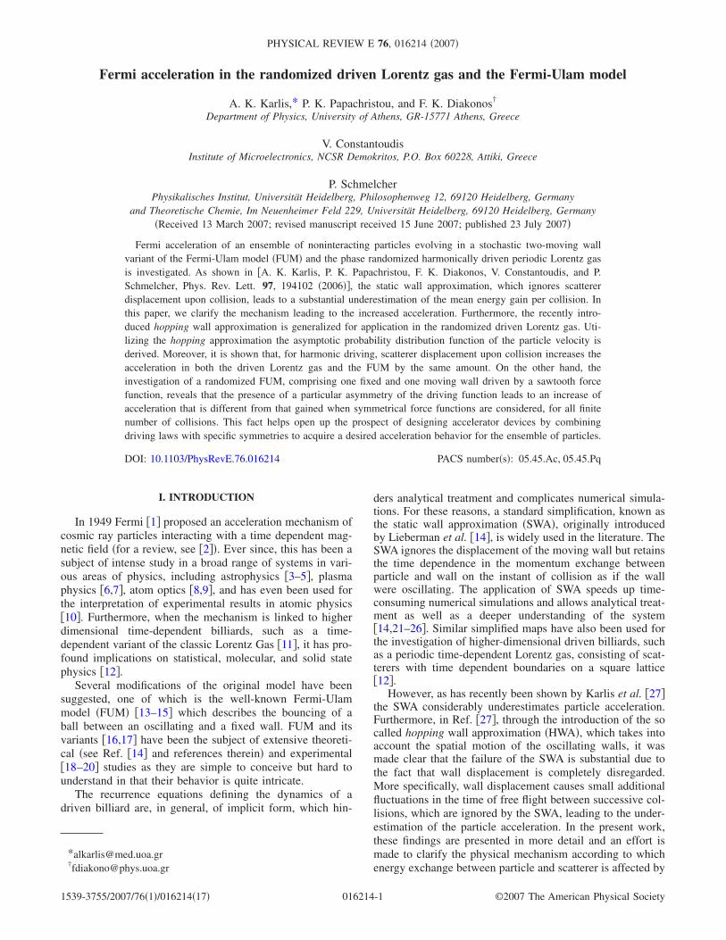
particles, for n=5105 collisions, with �=1/15 and V0=100/15 are presented in Fig. 1 along with numerical resultsusing the exact Eqs. �1� and �2�. Clearly, and despite theexternal randomization �14� the SWA fails to provide an ac-curate description of the acceleration process; more specifi-cally, the energy gain of the particles is substantially under-estimated. The shortcomings of the SWA must be attributedto the fact that it does not take into account the displacementof the scatterer upon collision. Thus, it is crucial, in order to

correctly describe the evolution of the root mean square par-ticle velocity, to incorporate the oscillation of the walls inconfiguration space.

B. Hopping wall approximation

As mentioned above, one of the advantages of the SWA isthe explicit form of Eqs. �3a� and �3b�, which facilitates theanalytical treatment of the acceleration problem as well assubstantially simplifies and speeds up numerical simulations.Therefore, a promising candidate as an alternative to thisapproximation should also have these merits but at the sametime being capable of providing an accurate description ofthe acceleration process.

For this reason we introduce the so-called hopping wallapproximation �HWA�, which takes into account the effect ofthe wall displacement. Using this approximation we clarifyhow the oscillation of the wall in configuration space affectsthe acceleration law of an ensemble of particles. Further-more, the corresponding map allows an analytical treatmentand is as computationally efficient as the SWA, enabling usto calculate the evolution of the velocity distribution of theparticles for long time periods.

The key simplifying assumption of the HWA is that thewall position on the nth collision can be approximated withits position at the previous, �n−1�th, collision. This approxi-mation is based on the observation that with increasing par-ticle velocity, the time of free flight decreases, becomingmuch smaller compared to the oscillation period of the wallsand consequently the relative displacement of the wall be-tween two successive collisions becomes very small, i.e.,negligible. So, according to the HWA, one wall moves onlywhen a particle collides with the other wall. Thus, when aparticle collides with one of the walls, the other “hops” �isinstantly moved� to its new position �as defined by the deter-ministic and random phase component� and remains fixeduntil the particle collides again with the other wall. However,the velocity of both walls is allowed to oscillate continu-ously. The equations defining the HWA read

dn,�L,R� = �1

2+ � sin�tn−1 + �n� , �7a�

un = � cos�tn + �n� , �7b�

Vn = ± �− Vn−1 + 2un� . �7c�

As already mentioned in Sec. II A, the absolute value in Eq.�7c� is introduced in order to prevent the particle from trav-eling beyond the walls. The plus �minus� sign corresponds toa collision with the left �right� wall. The time tn when the nthcollision occurs is determined by Eq. �2�, which within theframework of HWA can be solved analytically to obtain

tn = tn−1 + �tn* ±

1

Vn−1, �8a�

0 1 2 3 4 5

x 105

0

20

40

60

80

100

Number of collisions n

Vrm

s

FIG. 1. Numerical results for Vrms of an ensemble of 104 par-ticles evolving in a stochastic FUM with two oscillating walls as afunction of the number of collisions. Results were obtained by iter-ating the exact �� as well as the corresponding static �+� approxi-mate map, with �=1/15 and V0=100/15. Vrms is measured in unitsof �w. The analytical result according to the SWA, obtained byaveraging over the random phase �solid line�, is also shown.

FERMI ACCELERATION IN THE RANDOMIZED DRIVEN … PHYSICAL REVIEW E 76, 016214 �2007�

016214-3

�tn* =

��sin�tn−1 + �n� − sin�tn−2 + �n−1��Vn−1

, �8b�

where �tn* is the correction term to the time of free flight

predicted by SWA, due to wall displacement.In order to obtain the rms particle velocity within the

framework of HWA, the mean energy gain per collision��Vn

2� must be calculated. Let us first calculate the averageenergy gain over the phase of oscillation, ���Vn

2��. This isdone by averaging Eq. �4� over the random phase component�n, using the set of Eqs. �8a� and �8b�, which leads to thefollowing integrals:

Ij = 0

2� 1

2��� cos�tn + �n�� jd�n, �9�

where j=1, 2 and tn is given by Eq. �8a�. An exact analyticalcalculation of the integrals I1, I2 is not possible. However, forthe set of parameters considered here, �tn

* is much smallercompared to the other phase components. Therefore, we ex-pand the right-hand side �RHS� of Eq. �9� to the leadingorder of �tn

*, to obtain

I1 =1

2�

0

2� �� cos� 1

Vn−1+ tn−1 + �n

− � sin� 1

Vn−1+ tn−1 + �n �tn

*�d�n, �10�

I2 =1

2�

0

2� ��2 cos2� 1

Vn−1+ tn−1 + �n

− 2�2 cos� 1

Vn−1+ tn−1 + �n

sin� 1

Vn−1+ tn−1 + �n �tn

*�d�n. �11�

After the substitution of Eq. �8b� into Eqs. �10� and �11� thecalculation of the integrals yields

I1 � −

�2 cos� 1

Vn−1

2Vn−1, I2 �

�2

2.

Therefore, we find

���Vn2�� � 2�2 cos� 1

Vn−1 + 2�2. �12�

At the limit of high particle velocities Vn−1�1, Eq. �12� issimplified to, ���Vn

2���4�2. Since the result is independentof the particle velocity, the ensemble mean energy gain is

��Vn2� � 4�2, �13�

which is exactly two times the result obtained by neglectingwall displacement. Consequently, the root mean square ve-locity as a function of the number of collisions is

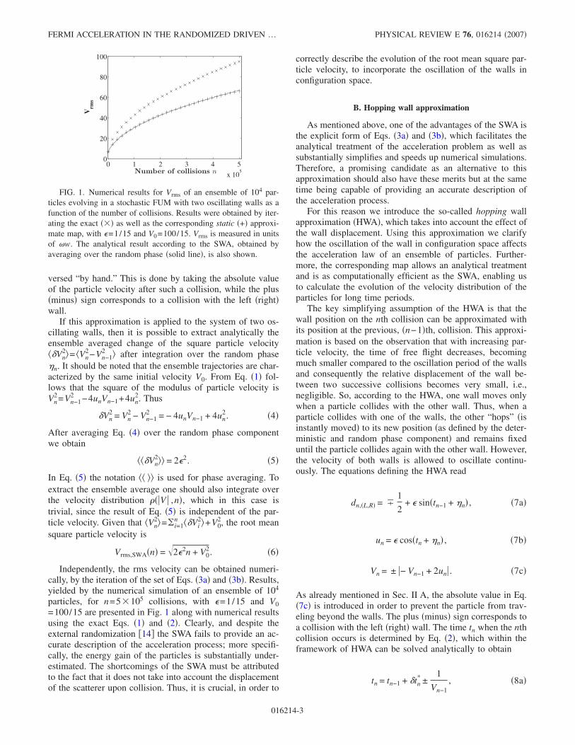
Vrms,HWA�n� = 4�2n + �V02� . �14�

The analytical result of Eq. �14� together with the numericalresults obtained by the simulation of 104 particles utilizingthe HWA map, are shown in Fig. 2. For the sake of compari-son, numerical results using the exact map are also pre-sented.

As seen in Fig. 2 the numerical results given by the itera-tion of the exact and the hopping approximative map virtu-ally coincide. Furthermore, the analytical result of Eq. �14� isalso in agreement with the numerical results obtained usingthe exact map. Obviously, the HWA succeeds in describingparticle acceleration, in clear contrast with the SWA whichleads to a substantial underestimation. This indicates that theincreased particle acceleration is due to the impact of thedynamically induced correlation between the position andvelocity of the oscillating wall in the collision process.

C. Physical mechanism

The previous analysis reveals the role of the fluctuationsin the time of flight �tn between successive collisions causedby the displacement of the scatterer. Despite the existence ofan external stochastic component in the phase of the oscil-lating wall these fluctuations lead to a systematic increase ofthe acceleration of the particles. A simple explanation of thephysical mechanism leading to the increased acceleration be-comes possible by considering the various configurations ofthe collision processes between the walls and the particles.

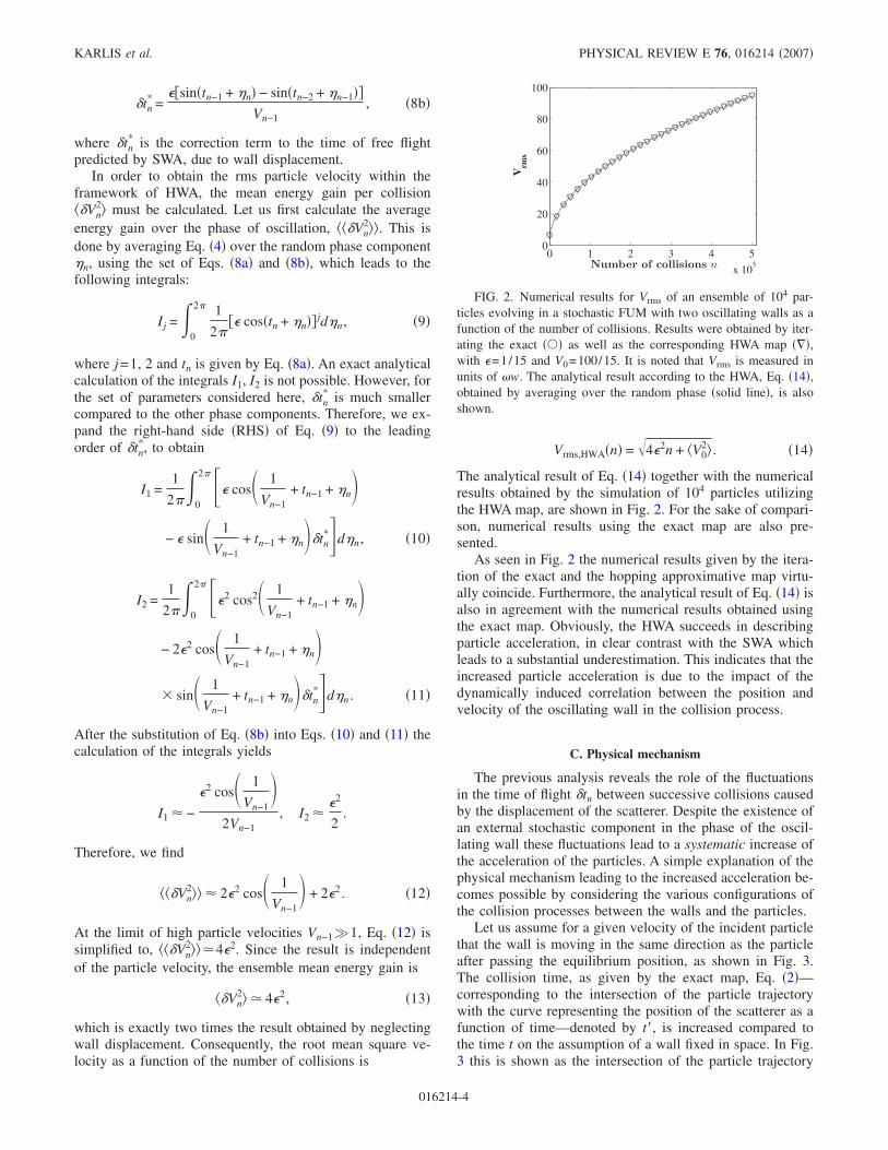
Let us assume for a given velocity of the incident particlethat the wall is moving in the same direction as the particleafter passing the equilibrium position, as shown in Fig. 3.The collision time, as given by the exact map, Eq. �2�—corresponding to the intersection of the particle trajectorywith the curve representing the position of the scatterer as afunction of time—denoted by t�, is increased compared tothe time t on the assumption of a wall fixed in space. In Fig.3 this is shown as the intersection of the particle trajectory

0 1 2 3 4 5

x 105

0

20

40

60

80

100

Number of collisions n

Vrm

s

FIG. 2. Numerical results for Vrms of an ensemble of 104 par-ticles evolving in a stochastic FUM with two oscillating walls as afunction of the number of collisions. Results were obtained by iter-ating the exact ��� as well as the corresponding HWA map ���,with �=1/15 and V0=100/15. It is noted that Vrms is measured inunits of �w. The analytical result according to the HWA, Eq. �14�,obtained by averaging over the random phase �solid line�, is alsoshown.

KARLIS et al. PHYSICAL REVIEW E 76, 016214 �2007�

016214-4

with the line corresponding to the equilibrium position. Inthis case, the velocity of the harmonically oscillating wall isa decreasing function of time and therefore an increase of thecollision time leads to a decrease of the wall velocity on theactual instant of the collision when compared to the staticwall approximation. This in turn leads to a reduced energyloss in the course of the collision. This reasoning holdsequally for all other types of collisional events, leading to thegeneral picture of reduced energy loss or enhanced energygain when the wall displacement is taken into account.

It should be stressed that although the additional fluctua-tions in the time of free flight due to wall displacement leadalways to an increased acceleration compared to the accel-eration predicted by the SWA, the specific amount of theincrease in the energy gain per collision due to the walldisplacement, depends on the characteristics of the oscilla-tion law. For this reason the ratio Rh�n�= ��Vn

2�− �V0

2��exact / ��Vn2�− �V0

2��SWA=�i=1n ��Vi

2�exact /�i=1n ��Vi

2�SWA isintroduced, which enables us to compare the relative effi-ciency of the mechanism leading to the increased accelera-tion between setups with different driving force laws. Thespecific definition of Rh�n�, compared to that given in Ref.�27�, is more convenient for numerical calculations as it con-verges much more rapidly in terms of ensemble averaging��105 initial conditions are adequate for reducing statisticaluncertainties to less that 1%, as opposed to numerical simu-lations using the definition of Rh�n� given in Ref. �27� inwhich case 106 initial conditions are necessary�. For theharmonically driven FUM �with randomized phase of oscil-lation� the correction factor Rh�n� can readily be calculatedusing Eqs. �5� and �12�, to obtain

Rh�n� =1

n�i=1

n �cos� 1

Vi−1 � + 1. �15�

Due to the Fermi acceleration mechanism developed in theFUM particle velocities quickly acquire large values, i.e.,

1 /V�1. The expansion of the right-hand side of Eq. �15� inpowers of 1 /V yields

Rh�n� = 2 + O�� 1

V2� . �16�

Consequently, in the case of the two-moving wall variant ofthe FUM driven by a harmonic driving force and randomizedphase of oscillation, the function Rh�n� is �within the leadingorder of �1/V� approximation� independent of n and equals2. It should be stressed that this result applies also to theoriginal FUM, with one fixed and one moving wall. Indeed,due to the randomization of the phase of oscillation and thesymmetry u�m�T /2�+T /4− t�=−u�m�T /2�+T /4+ t� �m=0,1 ,2 , . . . � of the oscillation time law, the two-wall variantof the FUM becomes fully equivalent to the original FUM,because collisions of the particles with either side of themoving wall�s�, on the average, result to the same energytransfer. However, we will show that this is not the casewhen this particular symmetry of the oscillation law is bro-ken.

D. Sawtooth driving law

In order to demonstrate the variability of the factor Rh andits dependence on the characteristics of the oscillation law,we perform an analysis of the case of a sawtooth driving law,in the context of the original FUM—consisting of one mov-ing and one fixed wall—as well as the two-moving wallFUM variant. In all occasions the phase of the oscillatingwall�s� is�are� shifted randomly �according to a uniform dis-tribution� after each collision with a particle. The followingclass of time-periodic laws for the moving wall�s� are con-sidered:

T/4 T/2 3T/2−A

−A/2

0

A/2

A

t

δt∗

δv Scatterer position

Scatterer velocity

Particle trajectory

t t′

FIG. 3. The position and thevelocity of one of the oscillatingwalls as a function of time. Thestraight line represents the trajec-tory of an incident particle.

FERMI ACCELERATION IN THE RANDOMIZED DRIVEN … PHYSICAL REVIEW E 76, 016214 �2007�

016214-5

xi�t� = x0,i +�1

a

�t + ��AT

,�t + ��

T� �0,a� ,

−2

b − a

�t + ��AT

,�t + ��

T� �a,b� ,

1

1 − b

�t + ��AT

,�t + ��

T� �b,1� ,

�17�

u�t� =�1

a

A

T,

�t + ��T

� �0,a� ,

−2

b − a

A

T,

�t + ��T

� �a,b� ,

1

1 − b

A

T,

�t + ��T

� �b,1� ,

�18�

where T is the period of the oscillation, A the amplitude,x0,�L,R� the equilibrium position of the left or right movingwall and � a random number uniformly distributed in�0,2��. Despite the randomization of the phase of oscilla-tion, due to the breaking of the symmetry u�m�T /2�+T /4− t�=−u�m�T /2�+T /4+ t� �m=0,1 ,2 , . . . �, the accelerationrate in a FUM with one oscillating and one fixed wall and ina two-moving wall FUM is not identical. To clarify this, letus calculate the factor Rh,i�n� �i=L ,R� in each setup, begin-ning from the FUM with one vibrating wall at x=0 and afixed wall at x=w.

The change of the particle square velocity on the nth col-lision is given by the expression

�Vn2 = Vn

2 − Vn−12 = − 4Vnun + 4un

2, �19�

where un is the wall velocity upon the nth collision and Vn−1is the particle velocity before this collision. The parametersa, b control the asymmetry of xL�t�. In order to calculate theaverage over the phase ���Vn

2�� within the framework of theSWA we need to separate the ensemble of particle trajecto-ries in two sets. The first set consists of trajectories for whichthe acceleration process is identical to that of the exactmodel. The second set consists of trajectories for which theacceleration in the SWA is underestimated. Each zone ischaracterized by a fixed value of ���Vn

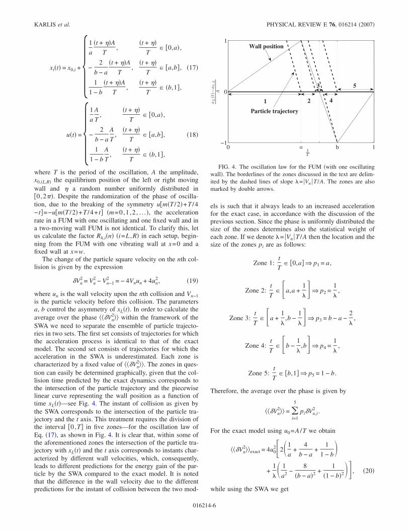
2��. The zones in ques-tion can easily be determined graphically, given that the col-lision time predicted by the exact dynamics corresponds tothe intersection of the particle trajectory and the piecewiselinear curve representing the wall position as a function oftime xL�t�—see Fig. 4. The instant of collision as given bythe SWA corresponds to the intersection of the particle tra-jectory and the t axis. This treatment requires the division ofthe interval �0,T� in five zones—for the oscillation law ofEq. �17�, as shown in Fig. 4. It is clear that, within some ofthe aforementioned zones the intersection of the particle tra-jectory with xL�t� and the t axis corresponds to instants char-acterized by different wall velocities, which, consequently,leads to different predictions for the energy gain of the par-ticle by the SWA compared to the exact model. It is notedthat the difference in the wall velocity due to the differentpredictions for the instant of collision between the two mod-

els is such that it always leads to an increased accelerationfor the exact case, in accordance with the discussion of theprevious section. Since the phase is uniformly distributed thesize of the zones determines also the statistical weight ofeach zone. If we denote �= �Vn �T /A then the location and thesize of the zones pi are as follows:

Zone 1:t

T� �0,a� ⇒ p1 = a ,

Zone 2:t

T� �a,a +

1

�� ⇒ p2 =

1

�,

Zone 3:t

T� �a +

1

�,b −

1

�� ⇒ p3 = b − a −

2

�,

Zone 4:t

T� �b −

1

�,b� ⇒ p4 =

1

�,

Zone 5:t

T� �b,1� ⇒ p5 = 1 − b .

Therefore, the average over the phase is given by

���Vn2�� = �

i=1

5

pi�Vn,i2 .

For the exact model using u0=A /T we obtain

���Vn2��exact = 4u0

2�2�1

a+

4

b − a+

1

1 − b

+1

�� 1

a2 −8

�b − a�2 +1

�1 − b�2 � , �20�

while using the SWA we get

0 b 1−1

0

1

xL(t

)−x0

,L

A

tT

a

Wall position

Particle trajectory

1 2

3

4

5

FIG. 4. The oscillation law for the FUM �with one oscillatingwall�. The borderlines of the zones discussed in the text are delim-ited by the dashed lines of slope �= �Vn �T /A. The zones are alsomarked by double arrows.

KARLIS et al. PHYSICAL REVIEW E 76, 016214 �2007�

016214-6

���Vn2��SWA = 4u0

2�1

a+

4

b − a+

1

1 − b . �21�

Thus the function Rh�n� is

Rh,L�n� = 2 +F�a,b�

n�i=1

n1

�, �22�

with

F�a,b� =

1

a2 −8

�b − a�2 +1

�1 − b�2

1

a+

4

b − a+

1

1 − b

.

Now we can perform also the averaging over the velocitydistribution of the particles and obtain the final expression:

Rh,L�n� = 2 +u0F�a,b�

n�i=1

n � 1

�Vi−1�� . �23�

To derive a formula featuring explicitly the dependence on nit is necessary to determine �1/ �Vn−1 � � as a function of n.Since the FUM under discussion is randomized, the accelera-tion of the particles can be described as a diffusion process inmomentum space, i.e., by the Fokker-Planck equation. Thesolution of the Fokker-Planck equation �see Appendix A�assuming a perfectly reflective barrier at �V � =0 leads to thefollowing asymptotic �n�1� expression for �1/Vn−1�:

� 1

�Vn−1�� ��

2

1

�,

� =g�a,b��n − 1� +V0

2

2,

g�a,b� = 4u02�1

a+

4

b − a+

1

1 − b . �24�

The summation after the substitution of Eqs. �24� into Eq.�23� yields

Rh,L�n� = 2 +u0F�a,b�

n �

2g�a,b�� �1

2,

V02

2g�a,b�

− �1

2,n +

V02

2g�a,b� � , �25�

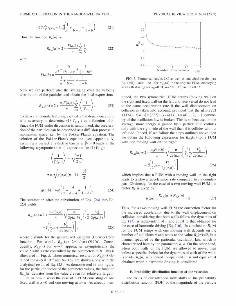
where stands for the generalized Riemann �Hurwitz� zetafunction. For n�1, Rh,L�n�−2�1/n+O�1/n�. Conse-quently, Rh,L�n� for n→� approaches asymptotically thevalue 2 with a rate controlled by the parameters a, b. This isillustrated in Fig. 5, where numerical results for Rh,L�n� ob-tained for a=510−3 and b=0.67 are shown along with theanalytical result of Eq. �25�. As demonstrated in this figure,for the particular choice of the parameter values, the functionRh,L�n� deviates from the value 2 even for relatively large n.

Let us now discuss the case of a FUM consisting of onefixed wall at x=0 and one moving at x=w. As already men-

tioned, the two symmetrical FUM setups �moving wall onthe right and fixed wall on the left and vice versa� do not leadto the same acceleration rate if the wall displacement oncollision is taken into account, provided that the u�m�T /2�+ �T /4�− t�=−u�m�T /2�+ �T /4�+ t�, �m=0,1 ,2 , . . . � symme-try of the oscillation law is broken. This is so because, on theaverage, more energy is gained by a particle if it collidesonly with the right side of the wall than if it collides with itsleft side. Indeed, if we follow the steps outlined above thenwe obtain the following expression for Rh,R�n� for a FUMwith one moving wall on the right:

Rh,R�n� = 2 −u0F�a,b�

n �

2g�a,b�� �1

2,

V02

2g�a,b�

− �1

2,n +

V02

2g�a,b� � , �26�

which implies that a FUM with a moving wall on the rightleads to a slower acceleration rate compared to its counter-part. Obviously, for the case of a two-moving wall FUM thefactor Rh is given by

Rh�n� =Rh,L�n� + Rh,R�n�

2= 2. �27�

Thus, for a two-moving wall FUM the correction factor forthe increased acceleration due to the wall displacement oncollision, considering that both walls follow the dynamics ofEq. �17�, is independent of n and equal to that obtained forthe case of harmonic driving �Eq. �16��. In conclusion, Rh�n�for the FUM setups with one moving wall depends on thenumber of collisions n and tends to the value Rh���=2, in amanner specified by the particular oscillation law, which ischaracterized here by the parameters a, b. On the other hand,when both walls of the FUM are allowed to move, thenunless a specific choice for the dynamics of each of the wallsis made, Rh�n� is rendered independent of n and equals thatobtained when a harmonic driving is considered.

E. Probability distribution function of the velocities

The focus of our attention now shifts to the probabilitydistribution function �PDF� of the magnitude of the particle

0.5 1 1.5 2

x 105

1.8

1.9

2

2.1

2.2

2.3

Number of collisions n

Rh,

L

FIG. 5. Numerical results �� as well as analytical results �seeEq. �25��—solid line—for Rh,L�n� in the original FUM, employingsawtooth driving for u0=0.01, a=510−3, and b=0.67.

FERMI ACCELERATION IN THE RANDOMIZED DRIVEN … PHYSICAL REVIEW E 76, 016214 �2007�

016214-7

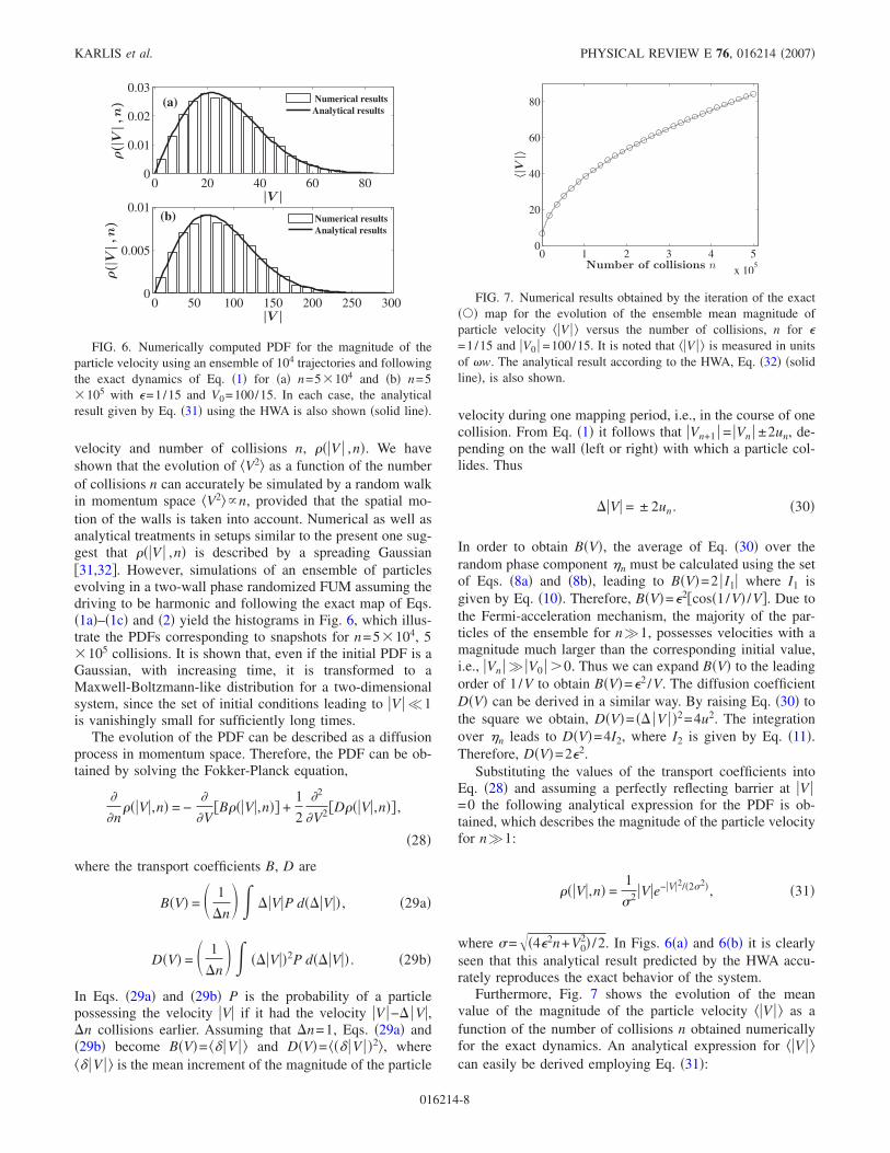
velocity and number of collisions n, ���V � ,n�. We haveshown that the evolution of �V2� as a function of the numberof collisions n can accurately be simulated by a random walkin momentum space �V2��n, provided that the spatial mo-tion of the walls is taken into account. Numerical as well asanalytical treatments in setups similar to the present one sug-gest that ���V � ,n� is described by a spreading Gaussian�31,32�. However, simulations of an ensemble of particlesevolving in a two-wall phase randomized FUM assuming thedriving to be harmonic and following the exact map of Eqs.�1a�–�1c� and �2� yield the histograms in Fig. 6, which illus-trate the PDFs corresponding to snapshots for n=5104, 5105 collisions. It is shown that, even if the initial PDF is aGaussian, with increasing time, it is transformed to aMaxwell-Boltzmann-like distribution for a two-dimensionalsystem, since the set of initial conditions leading to �V � �1is vanishingly small for sufficiently long times.

The evolution of the PDF can be described as a diffusionprocess in momentum space. Therefore, the PDF can be ob-tained by solving the Fokker-Planck equation,

�

�n���V�,n� = −

�

�V�B���V�,n�� +

1

2

�2

�V2 �D���V�,n�� ,

�28�

where the transport coefficients B, D are

B�V� = � 1

�n ��V�P d���V�� , �29a�

D�V� = � 1

�n ���V��2P d���V�� . �29b�

In Eqs. �29a� and �29b� P is the probability of a particlepossessing the velocity �V� if it had the velocity �V �−� �V�,�n collisions earlier. Assuming that �n=1, Eqs. �29a� and�29b� become B�V�= �� �V � � and D�V�= ��� �V � �2�, where�� �V � � is the mean increment of the magnitude of the particle

velocity during one mapping period, i.e., in the course of onecollision. From Eq. �1� it follows that �Vn+1 � = �Vn � ±2un, de-pending on the wall �left or right� with which a particle col-lides. Thus

��V� = ± 2un. �30�

In order to obtain B�V�, the average of Eq. �30� over therandom phase component �n must be calculated using the setof Eqs. �8a� and �8b�, leading to B�V�=2 � I1� where I1 isgiven by Eq. �10�. Therefore, B�V�=�2�cos�1/V� /V�. Due tothe Fermi-acceleration mechanism, the majority of the par-ticles of the ensemble for n�1, possesses velocities with amagnitude much larger than the corresponding initial value,i.e., �Vn � � �V0 � 0. Thus we can expand B�V� to the leadingorder of 1 /V to obtain B�V�=�2 /V. The diffusion coefficientD�V� can be derived in a similar way. By raising Eq. �30� tothe square we obtain, D�V�= �� �V � �2=4u2. The integrationover �n leads to D�V�=4I2, where I2 is given by Eq. �11�.Therefore, D�V�=2�2.

Substituting the values of the transport coefficients intoEq. �28� and assuming a perfectly reflecting barrier at �V �=0 the following analytical expression for the PDF is ob-tained, which describes the magnitude of the particle velocityfor n�1:

���V�,n� =1

�2 �V�e−�V�2/�2�2�, �31�

where �=�4�2n+V02� /2. In Figs. 6�a� and 6�b� it is clearly

seen that this analytical result predicted by the HWA accu-rately reproduces the exact behavior of the system.

Furthermore, Fig. 7 shows the evolution of the meanvalue of the magnitude of the particle velocity ��V � � as afunction of the number of collisions n obtained numericallyfor the exact dynamics. An analytical expression for ��V � �can easily be derived employing Eq. �31�:

0 20 40 60 800

0.01

0.02

0.03

|V |

ρ(|V

|,n) (a) Numerical results

Analytical results

0 50 100 150 200 250 3000

0.005

0.01

|V |

ρ(|V

|,n) (b) Numerical results

Analytical results

FIG. 6. Numerically computed PDF for the magnitude of theparticle velocity using an ensemble of 104 trajectories and followingthe exact dynamics of Eq. �1� for �a� n=5104 and �b� n=5105 with �=1/15 and V0=100/15. In each case, the analyticalresult given by Eq. �31� using the HWA is also shown �solid line�.

0 1 2 3 4 5

x 105

0

20

40

60

80

Number of collisions n

〈|V

|〉

FIG. 7. Numerical results obtained by the iteration of the exact��� map for the evolution of the ensemble mean magnitude ofparticle velocity ��V � � versus the number of collisions, n for �=1/15 and �V0 � =100/15. It is noted that ��V � � is measured in unitsof �w. The analytical result according to the HWA, Eq. �32� �solidline�, is also shown.

KARLIS et al. PHYSICAL REVIEW E 76, 016214 �2007�

016214-8

��V�� =��4�2n + V0

2�2

. �32�

For the sake of comparison this analytical result is also pre-sented in Fig. 7. Once again, results yielded by the exact andthe HWA map are in excellent agreement.

III. TIME-DEPENDENT LORENTZ GAS

In the theory of dynamical systems Lorentz gas �11� actsas a paradigm allowing us to address fundamental issues ofstatistical mechanics, for instance, ergodicity and mixing�33–35� and transport processes, such as diffusion in con-figuration space �36–41�. A generalization of the original pe-riodic Lorentz gas model has recently been introduced �12�allowing the velocity of the scatterers to oscillate radially ona square lattice, i.e., static approximation. Due to the inher-ent strong chaotic dynamics of the static Lorentz gas, owingto the convex geometry of the scatterers, one intuitively ex-pects �22� that the introduction of time dependence induces aFermi mechanism of acceleration, resulting in unboundedgrowth of the velocity of the tracer particle. This is in con-trast to the FUM, where, on the supposition of smooth peri-odic force functions, the particle energy remains bounded,due to the presence of a set of spanning KAM curves in thephase space �14,15� and only in the presence of externalstochasticity does Fermi acceleration become feasible.

In the following, we study a time-dependent Lorentz gasconsisting of harmonically oscillating scatterers on a triangu-lar lattice. For this specific geometry, the horizon, i.e., themaximum distance traveled by an incident particle withoutsuffering a collision, is finite �36�, provided that the spacingw between neighboring disks is appropriately chosen. Asmentioned above stochasticity is not needed in order to studyFermi acceleration. However, as will be shown, the presenceor absence of stochasticity, as well as the specific manner inwhich it is introduced affects the acceleration process. Thehigher dimensionality of the system, in comparison to that ofthe FUM, provides us with another way to induce stochas-ticity without affecting the energy of the oscillating scatterersapart from phase randomization, namely by randomizing thedirection of the oscillation axis. Therefore, stochasticity isinduced by �a� performing a random phase shift to all scat-terers when an incident particle exits the scattering area,through the addition of a random, uniformly distributed num-ber �� �0,2�� or by �b� rotating randomly the oscillationaxis of all scatterers when again the particle exits the scat-tering area of the disk with which it collided; specifically, theinclination angle of the axis of oscillation of each disk isuniformly distributed in �0,��. The imposed stochasticitysimulates the effect of thermal fluctuations on the dynamicsof the considered system. It is emphasized that the specificvalues of the random phase � or the axis inclination angles �are updated once the particles escape the hexagonal elemen-tary cell of the lattice. Within this approximation, memoryeffects are absent, and the simulation of thermal noise iseasily implemented.

Although the static approximation has been successfullyused in the past to understand the power-law increase of the

mean velocity in a time-dependent Lorentz gas �12� it hasalso been shown that this approximation fails to describecorrectly the increase of the mean particle velocity �27� inthe case of a phase randomized harmonically driven periodicLorentz gas, i.e., it systematically underestimates the numeri-cally observed acceleration. However, motivated by the goodagreement between the numerical results of the exact and theso called hopping map in Ref. �27� we utilize the latter in aneffort to understand the dynamical correlations that lead to ahigher acceleration in the harmonically driven Lorentz gas.

A. Exact map

The dynamics of a point particle suffering elastic colli-sions with a circular infinitely heavy harmonically drivenscatterer are described by the following set of equations �42�:

0 = c1�tn − tn−1�2 + c2 sin2��tn + �n� + c3�tn − tn−1�

+ sin��tn + �n� + c4�tn − tn−1� + c5 sin��tn + �n� + c6,

�33a�

rn = rn−1 + Vn−1�tn − tn−1� , �33b�

un,i = Ai� cos��tn + �n� , �33c�

Vn = Vn−1 − 2�n�Vn−1 − un��n , �33d�

where Ai is a vector directed along the randomly chosen axisof oscillation with magnitude equal to the amplitude of theoscillation of the ith scatterer, � is the angular frequency ofoscillation, �n is a random number uniformly distributed inthe interval �0,2��, tn is the instant when the nth collisionoccurs, rn the position vector of the particle at the instant tn,Vn the particle velocity vector immediately after the colli-sion, un the velocity of the scatterer, and finally n the inwardnormal vector at the point of collision on the scatterer’sboundary where collision occurs. Parameters c1 , . . . ,c6 aregiven by

c1 = Vn−12 ,

c2 = �Ai�2,

c3 = − 2Vn−1 · Ai,

c4 = 2�rn−1 − d0,i� · Vn−1,

c5 = 2�rn−1 − d0,i� · Vn−1,

c6 = �rn−1 − d0,i�2 − �Ri�2,

where d0,i is the position vector of the center of the ith scat-terer at equilibrium and Ri its radius. For the sake of simplic-ity in the present analysis we assume that all the scatterershave the same amplitude of oscillation and radii. In order toeliminate the nonrelevant parameters, the dimensionlessquantity �= �A � /w is introduced, where w denotes the spac-ing between the disk centers. Using as a length unit w and as

FERMI ACCELERATION IN THE RANDOMIZED DRIVEN … PHYSICAL REVIEW E 76, 016214 �2007�

016214-9

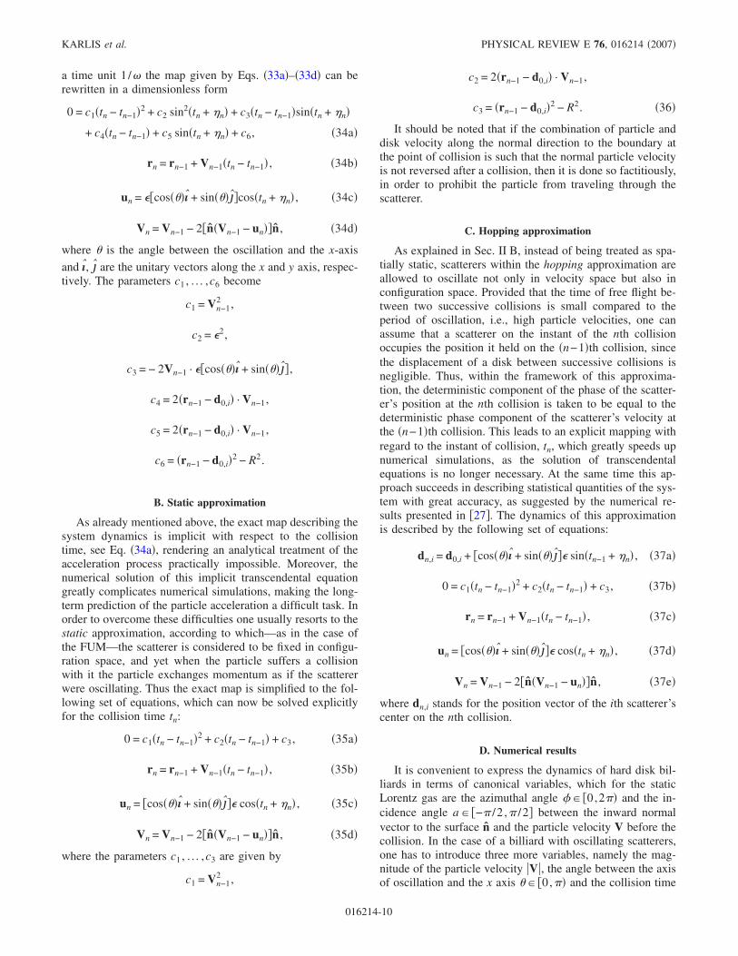
a time unit 1 /� the map given by Eqs. �33a�–�33d� can berewritten in a dimensionless form

0 = c1�tn − tn−1�2 + c2 sin2�tn + �n� + c3�tn − tn−1�sin�tn + �n�

+ c4�tn − tn−1� + c5 sin�tn + �n� + c6, �34a�

rn = rn−1 + Vn−1�tn − tn−1� , �34b�

un = ��cos���ı + sin���j�cos�tn + �n� , �34c�

Vn = Vn−1 − 2�n�Vn−1 − un��n , �34d�

where � is the angle between the oscillation and the x-axis

and ı, j are the unitary vectors along the x and y axis, respec-tively. The parameters c1 , . . . ,c6 become

c1 = Vn−12 ,

c2 = �2,

c3 = − 2Vn−1 · ��cos���ı + sin���j� ,

c4 = 2�rn−1 − d0,i� · Vn−1,

c5 = 2�rn−1 − d0,i� · Vn−1,

c6 = �rn−1 − d0,i�2 − R2.

B. Static approximation

As already mentioned above, the exact map describing thesystem dynamics is implicit with respect to the collisiontime, see Eq. �34a�, rendering an analytical treatment of theacceleration process practically impossible. Moreover, thenumerical solution of this implicit transcendental equationgreatly complicates numerical simulations, making the long-term prediction of the particle acceleration a difficult task. Inorder to overcome these difficulties one usually resorts to thestatic approximation, according to which—as in the case ofthe FUM—the scatterer is considered to be fixed in configu-ration space, and yet when the particle suffers a collisionwith it the particle exchanges momentum as if the scattererwere oscillating. Thus the exact map is simplified to the fol-lowing set of equations, which can now be solved explicitlyfor the collision time tn:

0 = c1�tn − tn−1�2 + c2�tn − tn−1� + c3, �35a�

rn = rn−1 + Vn−1�tn − tn−1� , �35b�

un = �cos���ı + sin���j�� cos�tn + �n� , �35c�

Vn = Vn−1 − 2�n�Vn−1 − un��n , �35d�

where the parameters c1 , . . . ,c3 are given by

c1 = Vn−12 ,

c2 = 2�rn−1 − d0,i� · Vn−1,

c3 = �rn−1 − d0,i�2 − R2. �36�

It should be noted that if the combination of particle anddisk velocity along the normal direction to the boundary atthe point of collision is such that the normal particle velocityis not reversed after a collision, then it is done so factitiously,in order to prohibit the particle from traveling through thescatterer.

C. Hopping approximation

As explained in Sec. II B, instead of being treated as spa-tially static, scatterers within the hopping approximation areallowed to oscillate not only in velocity space but also inconfiguration space. Provided that the time of free flight be-tween two successive collisions is small compared to theperiod of oscillation, i.e., high particle velocities, one canassume that a scatterer on the instant of the nth collisionoccupies the position it held on the �n−1�th collision, sincethe displacement of a disk between successive collisions isnegligible. Thus, within the framework of this approxima-tion, the deterministic component of the phase of the scatter-er’s position at the nth collision is taken to be equal to thedeterministic phase component of the scatterer’s velocity atthe �n−1�th collision. This leads to an explicit mapping withregard to the instant of collision, tn, which greatly speeds upnumerical simulations, as the solution of transcendentalequations is no longer necessary. At the same time this ap-proach succeeds in describing statistical quantities of the sys-tem with great accuracy, as suggested by the numerical re-sults presented in �27�. The dynamics of this approximationis described by the following set of equations:

dn,i = d0,i + �cos���ı + sin���j�� sin�tn−1 + �n� , �37a�

0 = c1�tn − tn−1�2 + c2�tn − tn−1� + c3, �37b�

rn = rn−1 + Vn−1�tn − tn−1� , �37c�

un = �cos���ı + sin���j�� cos�tn + �n� , �37d�

Vn = Vn−1 − 2�n�Vn−1 − un��n , �37e�

where dn,i stands for the position vector of the ith scatterer’scenter on the nth collision.

D. Numerical results

It is convenient to express the dynamics of hard disk bil-liards in terms of canonical variables, which for the staticLorentz gas are the azimuthal angle �� �0,2�� and the in-cidence angle a� �−� /2 ,� /2� between the inward normalvector to the surface n and the particle velocity V before thecollision. In the case of a billiard with oscillating scatterers,one has to introduce three more variables, namely the mag-nitude of the particle velocity �V�, the angle between the axisof oscillation and the x axis �� �0,�� and the collision time

KARLIS et al. PHYSICAL REVIEW E 76, 016214 �2007�

016214-10

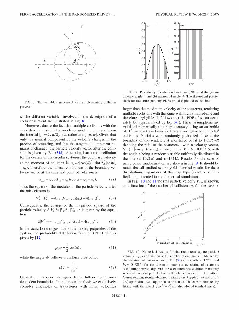
t. The different variables involved in the description of acollisional event are illustrated in Fig. 8.

Moreover, due to the fact that multiple collisions with thesame disk are feasible, the incidence angle a no longer lies inthe interval �−� /2 ,� /2�, but rather a� �−� ,��. Given thatonly the normal component of the velocity changes in theprocess of scattering, and that the tangential component re-mains unchanged, the particle velocity vector after the colli-sion is given by Eq. �34d�. Assuming harmonic oscillationfor the centers of the circular scatterers the boundary velocity

at the moment of collision is un=��cos���ı+sin���j�cos�tn

+�n�. Therefore, the normal component of the boundary ve-locity vector at the time and point of collision is

u�,n = � cos�tn + �n�cos�� − �n + �n� . �38�

Thus the square of the modulus of the particle velocity afterthe nth collision is

Vn2 = Vn−1

2 − 4u�,nVn−1 cos�an� + 4�u�,n�2. �39�

Consequently, the change of the magnitude square of theparticle velocity � �Vn�2= �Vn�2− �Vn−1�2 is given by the equa-tion

��V�2 = − 4u�,nVn−1 cos�an� + 4�u�,n�2. �40�

In the static Lorentz gas, due to the mixing properties of thesystem, the probability distribution function �PDF� of a isgiven by �12�

��a� =1

2cos�a� , �41�

while the angle �, follows a uniform distribution

���� =1

2�. �42�

Generally, this does not apply for a billiard with time-dependent boundaries. In the present analysis we exclusivelyconsider ensembles of trajectories with initial velocities

larger than the maximum velocity of the scatterers, renderingmultiple collisions with the same wall highly improbable andtherefore negligible. It follows that the PDF of a can accu-rately be approximated by Eq. �41�. These assumptions arevalidated numerically to a high accuracy, using an ensembleof 105 particle trajectories each one investigated for up to 104

collisions. Particles were randomly positioned close to theboundary of the scatterer, at a distance equal to 1.03R –Rdenoting the radii of the scatterers—with a velocity vector,V= ��V �cos z , �V �sin z�, of magnitude �V � =V=100/215, withthe angle z being a random variable uniformly distributed inthe interval �0,2�� and �=1/215. Results for the case ofusing phase randomization are shown in Fig. 9. It should benoted that all studied setups yield identical results for thesedistributions, regardless of the map type �exact or simpli-fied�, implemented in the numerical simulations.

In Figs. 10 and 11 the rms particle velocity Vrms is shown,as a function of the number of collisions n, for the case of

FIG. 8. The variables associated with an elementary collisionprocess.

−0.5 0 0.50

0.1

0.2

0.3

0.4

0.5

0.6

0.7

0.8

a/π

ρ(a

)

(a)

0 1 20

0.02

0.04

0.06

0.08

0.1

0.12

0.14

0.16

0.18

φ/π

ρ(φ

)

(b)

FIG. 9. Probability distribution functions �PDFs� of the �a� in-cidence angle a and �b� azimuthal angle �. The theoretical predic-tions for the corresponding PDFs are also plotted �solid line�.

1 2 3 4 5

x 105

0

1

2

3

4

5

Number of collisions n

Vrm

s

FIG. 10. Numerical results for the root mean square particlevelocity Vrms as a function of the number of collisions n obtained bythe iteration of the exact map, Eq. �34� ��� �with �=1/215 andV0=100/215� for the driven Lorentz gas consisting of scatterersoscillating horizontally, with the oscillation phase shifted randomlywhen an incident particle leaves the elementary cell of the lattice.Corresponding results obtained utilizing the hopping �+� and static�� approximative maps are also presented. The curves obtained byfitting with the model ��2n+V0

2 are also plotted �dashed lines�.

FERMI ACCELERATION IN THE RANDOMIZED DRIVEN … PHYSICAL REVIEW E 76, 016214 �2007�

016214-11

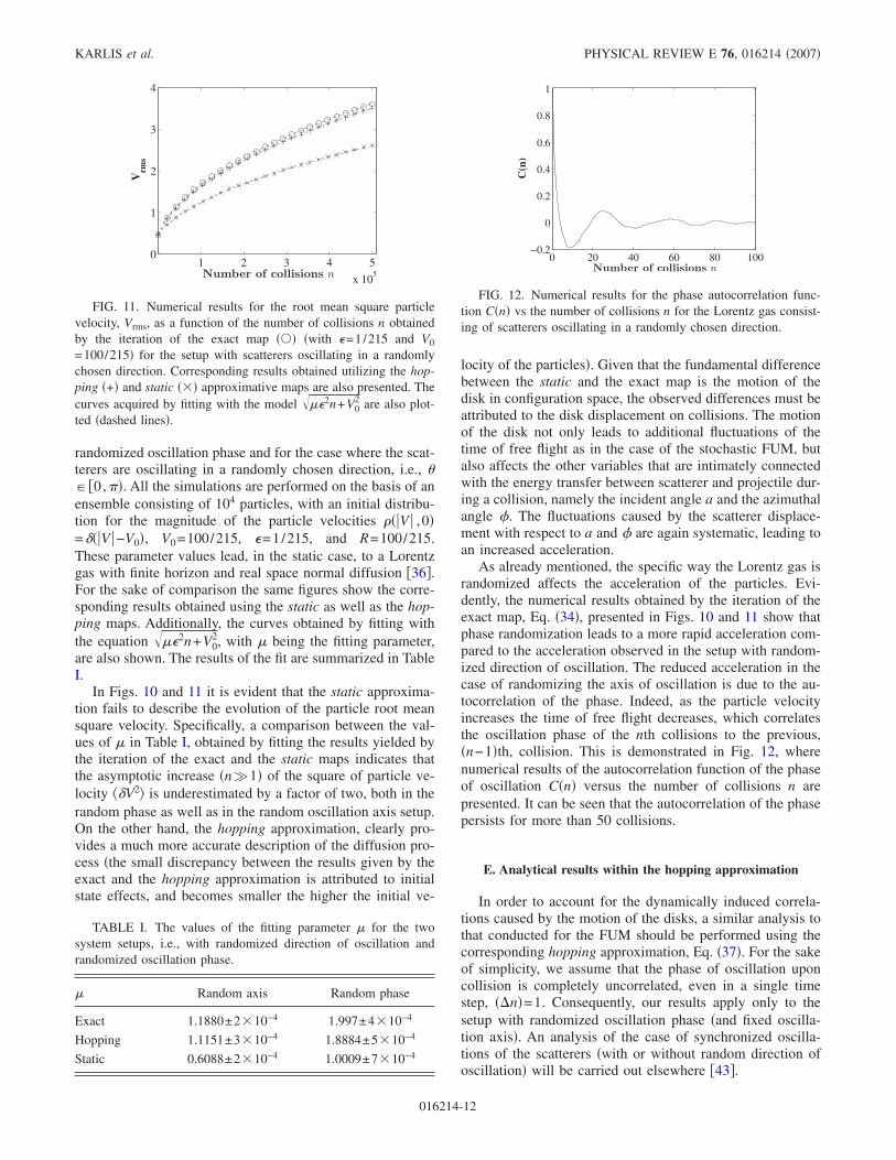
randomized oscillation phase and for the case where the scat-terers are oscillating in a randomly chosen direction, i.e., �� �0,��. All the simulations are performed on the basis of anensemble consisting of 104 particles, with an initial distribu-tion for the magnitude of the particle velocities ���V � ,0�=���V �−V0�, V0=100/215, �=1/215, and R=100/215.These parameter values lead, in the static case, to a Lorentzgas with finite horizon and real space normal diffusion �36�.For the sake of comparison the same figures show the corre-sponding results obtained using the static as well as the hop-ping maps. Additionally, the curves obtained by fitting withthe equation ��2n+V0

2, with � being the fitting parameter,are also shown. The results of the fit are summarized in TableI.

In Figs. 10 and 11 it is evident that the static approxima-tion fails to describe the evolution of the particle root meansquare velocity. Specifically, a comparison between the val-ues of � in Table I, obtained by fitting the results yielded bythe iteration of the exact and the static maps indicates thatthe asymptotic increase �n�1� of the square of particle ve-locity ��V2� is underestimated by a factor of two, both in therandom phase as well as in the random oscillation axis setup.On the other hand, the hopping approximation, clearly pro-vides a much more accurate description of the diffusion pro-cess �the small discrepancy between the results given by theexact and the hopping approximation is attributed to initialstate effects, and becomes smaller the higher the initial ve-

locity of the particles�. Given that the fundamental differencebetween the static and the exact map is the motion of thedisk in configuration space, the observed differences must beattributed to the disk displacement on collisions. The motionof the disk not only leads to additional fluctuations of thetime of free flight as in the case of the stochastic FUM, butalso affects the other variables that are intimately connectedwith the energy transfer between scatterer and projectile dur-ing a collision, namely the incident angle a and the azimuthalangle �. The fluctuations caused by the scatterer displace-ment with respect to a and � are again systematic, leading toan increased acceleration.

As already mentioned, the specific way the Lorentz gas israndomized affects the acceleration of the particles. Evi-dently, the numerical results obtained by the iteration of theexact map, Eq. �34�, presented in Figs. 10 and 11 show thatphase randomization leads to a more rapid acceleration com-pared to the acceleration observed in the setup with random-ized direction of oscillation. The reduced acceleration in thecase of randomizing the axis of oscillation is due to the au-tocorrelation of the phase. Indeed, as the particle velocityincreases the time of free flight decreases, which correlatesthe oscillation phase of the nth collisions to the previous,�n−1�th, collision. This is demonstrated in Fig. 12, wherenumerical results of the autocorrelation function of the phaseof oscillation C�n� versus the number of collisions n arepresented. It can be seen that the autocorrelation of the phasepersists for more than 50 collisions.

E. Analytical results within the hopping approximation

In order to account for the dynamically induced correla-tions caused by the motion of the disks, a similar analysis tothat conducted for the FUM should be performed using thecorresponding hopping approximation, Eq. �37�. For the sakeof simplicity, we assume that the phase of oscillation uponcollision is completely uncorrelated, even in a single timestep, ��n�=1. Consequently, our results apply only to thesetup with randomized oscillation phase �and fixed oscilla-tion axis�. An analysis of the case of synchronized oscilla-tions of the scatterers �with or without random direction ofoscillation� will be carried out elsewhere �43�.

TABLE I. The values of the fitting parameter � for the twosystem setups, i.e., with randomized direction of oscillation andrandomized oscillation phase.

� Random axis Random phase

Exact 1.1880±210−4 1.997±410−4

Hopping 1.1151±310−4 1.8884±510−4

Static 0.6088±210−4 1.0009±710−4

1 2 3 4 5

x 105

0

1

2

3

4

Number of collisions n

Vrm

s

FIG. 11. Numerical results for the root mean square particlevelocity, Vrms, as a function of the number of collisions n obtainedby the iteration of the exact map ��� �with �=1/215 and V0

=100/215� for the setup with scatterers oscillating in a randomlychosen direction. Corresponding results obtained utilizing the hop-ping �+� and static �� approximative maps are also presented. Thecurves acquired by fitting with the model ��2n+V0

2 are also plot-ted �dashed lines�.

0 20 40 60 80 100−0.2

0

0.2

0.4

0.6

0.8

1

Number of collisions n

C(n

)

FIG. 12. Numerical results for the phase autocorrelation func-tion C�n� vs the number of collisions n for the Lorentz gas consist-ing of scatterers oscillating in a randomly chosen direction.

KARLIS et al. PHYSICAL REVIEW E 76, 016214 �2007�

016214-12

Obviously, the disk displacement causes a shift of the val-ues of the incident angle a, the azimuthal angle � and thelength of the free path l traveled by the incident particle onits collision course to a disk. This leads to a shift of the timeof free flight �t= l / �V�. Therefore, assuming that the respec-tive values of the variables on the nth collision, were the diskto be fixed on its equilibrium position, are an, �n, and ln, Eqs.�38� and �40� can be rewritten as

��Vn�2 = − 4u�,nVn−1 cos�an + �an� + 4u�,n2 , �43�

u�,n = − � cos�tn−1 +ln + �ln

Vn+ �n cos��n + ��n� , �44�

where �an, ��n, and �ln denote the change to the values ofthe respective variables caused by the displacement of thescatterer on the nth collision. From geometrical consider-ations �an, ��n, and �ln can be expressed as a function of an,�n, ln,

�ln = R�cos��n� − cos��n + ��n� −�

Rsin�tn−1 + �n��

sec�an + �n� , �45�

sin�an + �an� = sin�an� −�

Rsin�tn−1 + �n�sin�an + �n� ,

�46�

��n = − �an. �47�

On the supposition of small oscillations the change �an, ��n,�ln caused by disk displacement to the angle variables and tothe free particle path is small, i.e., �an, ��n, �ln�1. There-fore, we can expand the left-hand side �LHS� of Eq. �46� tothe leading order of �an to obtain an explicit equation for�an:

�an = −�

Rsec�an�sin�tn−1 + �n�sin�an + �n� . �48�

After the substitution of Eqs. �45�, �47�, and �48� to Eq. �43�and integration over �, �, and a �for details see AppendixB�, assuming that they follow the PDFs defined by Eqs. �41�and �42�, we obtain a formula for the mean particle energygain upon a collision, which reads

�Vn2 = �2 cos� �l�

Vn + �2, �49�

where �l� stands for the mean free path on the supposition offixed scatterers at their corresponding equilibrium positions.In the limit of high particle velocities cos��l� /Vn� tends tounity. Thus the following asymptotic value of �V2 is ob-tained:

�Vn2 � 2�2. �50�

It follows that the rms particle velocity is

�Vn2� =�

j=1

n

���V� j2� + V0

2 = 2�2n + V02. �51�

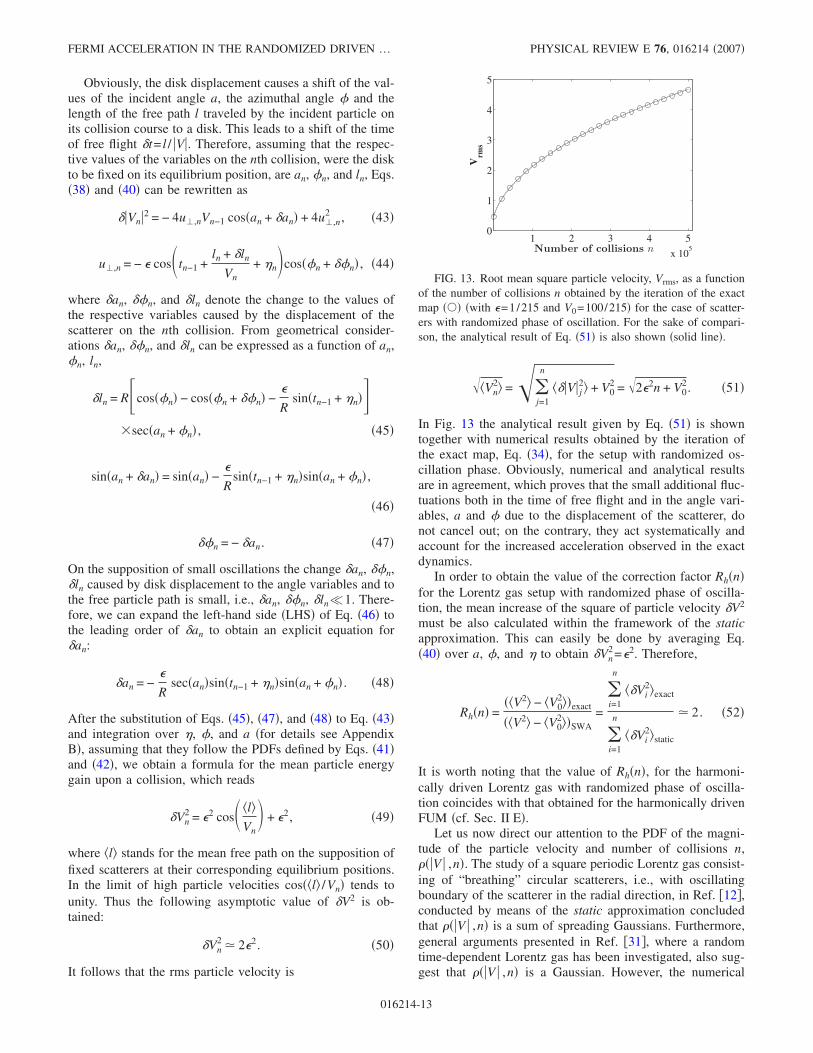
In Fig. 13 the analytical result given by Eq. �51� is showntogether with numerical results obtained by the iteration ofthe exact map, Eq. �34�, for the setup with randomized os-cillation phase. Obviously, numerical and analytical resultsare in agreement, which proves that the small additional fluc-tuations both in the time of free flight and in the angle vari-ables, a and � due to the displacement of the scatterer, donot cancel out; on the contrary, they act systematically andaccount for the increased acceleration observed in the exactdynamics.

In order to obtain the value of the correction factor Rh�n�for the Lorentz gas setup with randomized phase of oscilla-tion, the mean increase of the square of particle velocity �V2

must be also calculated within the framework of the staticapproximation. This can easily be done by averaging Eq.�40� over a, �, and � to obtain �Vn

2=�2. Therefore,

Rh�n� =��V2� − �V0

2��exact

��V2� − �V02��SWA

=

�i=1

n

��Vi2�exact

�i=1

n

��Vi2�static

� 2. �52�

It is worth noting that the value of Rh�n�, for the harmoni-cally driven Lorentz gas with randomized phase of oscilla-tion coincides with that obtained for the harmonically drivenFUM �cf. Sec. II E�.

Let us now direct our attention to the PDF of the magni-tude of the particle velocity and number of collisions n,���V � ,n�. The study of a square periodic Lorentz gas consist-ing of “breathing” circular scatterers, i.e., with oscillatingboundary of the scatterer in the radial direction, in Ref. �12�,conducted by means of the static approximation concludedthat ���V � ,n� is a sum of spreading Gaussians. Furthermore,general arguments presented in Ref. �31�, where a randomtime-dependent Lorentz gas has been investigated, also sug-gest that ���V � ,n� is a Gaussian. However, the numerical

1 2 3 4 5

x 105

0

1

2

3

4

5

Number of collisions n

Vrm

s

FIG. 13. Root mean square particle velocity, Vrms, as a functionof the number of collisions n obtained by the iteration of the exactmap ��� �with �=1/215 and V0=100/215� for the case of scatter-ers with randomized phase of oscillation. For the sake of compari-son, the analytical result of Eq. �51� is also shown �solid line�.

FERMI ACCELERATION IN THE RANDOMIZED DRIVEN … PHYSICAL REVIEW E 76, 016214 �2007�

016214-13

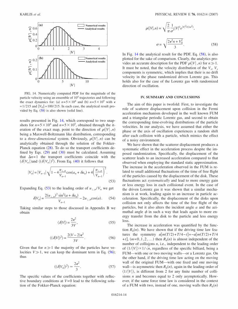
results presented in Fig. 14, which correspond to two snap-shots for n=5104 and n=5105, obtained through the it-eration of the exact map, point to the direction of ���V � ,n�being a Maxwell-Boltzmann like distribution, correspondingto a three-dimensional system. Obviously, ���V � ,n� can beanalytically obtained through the solution of the Fokker-Planck equation �28�. To do so the transport coefficients de-fined by Eqs. �29� and �30� must be calculated. Assumingthat �n=1 the transport coefficients coincide with the�� �Vn � �and ��� �Vn � �2�. From Eq. �40� it follows that

�Vn� = �Vn−1�1 − 4u�,n

Vn−1cos�an + �an� + 4� u�,n

Vn−1 2

.

�53�

Expanding Eq. �53� to the leading order of u�,n /Vn we get

��Vn� =2�u�,n�2 sin2�a + �an�

Vn−1− 2u�,ncos�a� . �54�

Taking similar steps to those discussed in Appendix B weobtain

���V�� =2�2

3V, �55�

����V��2� =2�V − 2��2

3V. �56�

Given that for n�1 the majority of the particles have ve-locities V�1, we can keep the dominant term in Eq. �56�;thus

����Vn��2� �2�2

3. �57�

The specific values of the coefficients together with reflec-tive boundary conditions at V=0 lead to the following solu-tion of the Fokker-Planck equation:

���V�,n� = 2

�

1

�3 �V�2e�V�2/�2�2�,

� =2�2n + V02

3. �58�

In Fig. 14 the analytical result for the PDF, Eq. �58�, is alsoplotted for the sake of comparison. Clearly, the analytics pro-vides an accurate description for the PDF ���V � ,n� for n�1.It must be noted, that the velocity distribution of the Vx, Vycomponents is symmetric, which implies that their is no driftvelocity in the phase randomized driven Lorentz gas. Thisholds also for the case of the Lorentz gas with randomizeddirection of oscillation.

IV. SUMMARY AND CONCLUSIONS

The aim of this paper is twofold: First, to investigate therole of scatterer displacement upon collision in the Fermiacceleration mechanism developed in the well known FUMand a triangular periodic Lorentz gas, and second to obtainthe corresponding time-evolving distributions of the particlevelocities. In our analysis, we have assumed that either thephase or the axis of oscillation experiences a random shiftafter each collision with a particle, which mimics the effectof a noisy environment.

We have shown that the scatterer displacement produces asystematic effect in the acceleration process despite the im-posed randomization. Specifically, the displacement of thescatterer leads to an increased acceleration compared to thatobserved when employing the standard static approximation.The increase in the acceleration observed in the FUM is re-lated to small additional fluctuations of the time of free flightof the particles caused by the displacement of the disk. Thesefluctuations act systematically and lead to more energy gainor less energy loss in each collisional event. In the case ofthe driven Lorentz gas it was shown that a similar mecha-nism is at work, leading again to an increase in particle ac-celeration. Specifically, the displacement of the disks uponcollision not only affects the time of the free flight of theparticles, but it also alters the incident angle a and the azi-muthal angle � in such a way that leads again to more en-ergy transfer from the disk to the particle and less energyloss.

The increase in acceleration was quantified by the func-tion Rh�n�. We have shown that if the driving time law fea-tures the symmetry u�m�T /2�+T /4− t�=−u�m�T /2�+T /4+ t�, �m=0,1 ,2 , . . . � then Rh�n� is almost independent of thenumber of collisions n, i.e., independent to the leading orderof �1/ �V � ��1/n, regardless of the specific billiard, being aFUM—with one or two moving walls—or a Lorentz gas. Onthe other hand, if the driving time law acting on the movingwall of the original FUM—with one fixed and one movingwall—is asymmetric then Rh�n�, again in the leading order of�1/ �V � �, is different from 2 for any finite number of colli-sions n and becomes equal to 2 only asymptotically. How-ever, if the same force time law is considered in the contextof a FUM with two, instead of one, moving walls then Rh�n�

0 1 2 3 40

0.2

0.4

0.6

|V |

ρ(|V

|,n) (a) Numerical results

Analytical results

0 5 100

0.1

0.2

|V |

ρ(|V

|,n) (b) Numerical results

Analytical results

FIG. 14. Numerically computed PDF for the magnitude of theparticle velocity using an ensemble of 104 trajectories and followingthe exact dynamics for: �a� n=5104 and �b� n=5105 with �=1/215 and �V0 � =100/215. In each case, the analytical result pro-vided by Eq. �58� is also shown �solid line�.

KARLIS et al. PHYSICAL REVIEW E 76, 016214 �2007�

016214-14

is again independent of the number of collisions n and equalsonce more 2.

The investigation of the distribution functions of particlevelocities in the FUM �with two moving walls or one mov-ing and one fixed� revealed that irrespective of the specificdriving of the billiard �sawtooth or harmonic� the same pro-file is obtained for n�1, resembling a 2D Maxwell-Boltzmann distribution. This is in contrast to the result ob-tained by the application of the standard SWA, i.e., by nottaking into account the displacement of the scatterer, wherethe corresponding PDFs are found spreading Gaussians.Moreover, we have shown that the application of the gener-alization of the hopping approximation leads to a similarprofile for the PDF in the case of higher dimensional bil-liards, such as the phase randomized harmonically drivenLorentz gas, in which case it was shown that the PDF of theparticle velocities is again Maxwell-Boltzmann-like �only inthis case corresponding to a higher dimensional system�. An-other interesting aspect of this finding is that, though in therandomized FUM billiards and in the driven Lorentz gas nosteady state of the distribution of the particle velocities ex-ists, in all circumstances, i.e., independently of the specificbilliard and driving, all the corresponding PDFs converge toa similar profile.

In all studied systems, we were able to obtain an analyti-cal estimation of the evolution of the mean square velocity ofthe particles as a function of the number of collisions n,independently of the derivation of the distribution of particlevelocities. For the setups considered herein it was found thatin the presence of external randomization, �V2�=Vrms�n.

As a final remark, we note that the understanding of thedependence of particle acceleration behavior on the symme-tries of the driving law, helps open up the prospect of design-ing specific devices combining driving laws with differentsymmetries in order to achieve a desired acceleration behav-ior.

ACKNOWLEDGMENT

The project is co-funded by the European Social Fund andNational Resources �EPEAEK II� PYTHAGORAS.

APPENDIX A: SOLUTION OF THE FOKKER-PLANCKEQUATION FOR THE SAWTOOTH DRIVEN FUM

The evolution of the PDF in a randomized billiard, asdiscussed in Sec. II E, can be determined by the Fokker-Planck �FP� equation. Therefore, to determine �1/ �V � � as afunction of the number of collisions, n, we must first obtainthe PDF by solving the FP equation,

�

�n���V�,n� = −

�

�V�B���V�,n�� +

1

2

�2

�V2 �D���V�,n�� ,

�A1�

where the transport coefficients B, D are

B�V� = � 1

�n ��V�P d���V�� , �A2a�

D�V� = � 1

�n ���V��2P d���V�� . �A2b�

Assuming �n=1 the coefficients B, D coincide with themean particle velocity increment � �V � � and the mean squareof the particle velocity increment ��� �V � �2�, respectively,whereas, � �V� is given by Eq. �30�. Therefore, to determinethe FP coefficients, the average of the wall velocity, ��un��and ��un

2�� over the oscillation phase must be calculated. Fol-lowing the steps thoroughly discussed in Sec. II D, one finds

B = ���V�� = 2u0

2

�V� �1

a+

4

b − a+

1

1 − b , �A3a�

D = ����V��2� = 4u02��1

a+

4

b − a+

1

1 − b

+u0

�V� � 1

a2 −8

�b − a�2 +1

�1 − b�2 � . �A3b�

Assuming the amplitude of wall velocity is small, u0

= AT �1 and at the limit of high particle velocities V�1 the

first term on the RHS of Eq. �A3b� dominates and the coef-ficient D��V � � becomes asymptotically equal to

D � 4u02�1

a+

4

b − a+

1

1 − b . �A4�

Assuming reflective boundary conditions at �V � =0 the solu-tion of Eq. �A1� is

���V�,n� =�V��2 e−�V�2/�2�2�, �A5�

where

� =4u02�1

a+

4

b − a+

1

1 − b n +

�V0�2

2.

Thus, �1/ �Vn � � as a function of the number of collisions, n,reads

� 1

�Vn�� =�

2

1

�. �A6�

APPENDIX B

Assuming that the amplitude of oscillation A is smallcompared to the radii of the scatterers R the change causedby disk displacement to the angle variables �an, ��n and tothe free particle path �ln is small, i.e., �an, ��n, �ln�1.Therefore, after the substitution of Eqs. �45� and �47� in Eq.�43�, we expand the RHS of the resulting equation to theleading order of �an to obtain

FERMI ACCELERATION IN THE RANDOMIZED DRIVEN … PHYSICAL REVIEW E 76, 016214 �2007�

016214-15

�Vn2 =

8 cos2��n�cos� ln

Vn−1+ �n + tn−1 sec�an + �n�sin��n + tn−1�sin� ln

Vn−1+ �n + tn−1 �3

Vn−1

+ 4 cos2��n�cos2� ln

Vn−1+ �n + tn−1 �2 + 4 cos�an�cos��n�sec�an + �n�sin��n + tn−1�sin� ln

Vn−1+ �n + tn−1 �2

+ 4Vn−1cos�an�cos��n�cos� ln

Vn−1+ �n + tn−1 �

+ �an�16 cos��n�cos� ln

Vn−1+ �n + tn−1 sec�an + �n�sin��n�sin��n + tn−1�

Vn−1�

sin� ln

Vn−1+ �n + tn−1 �3 + 8 cos��n�cos2� ln

Vn−1+ �n + tn−1 sin��n��2

+

8R cos2��n�cos� ln

Vn−1+ �n + tn−1 sec�an + �n�sin��n�sin� ln

Vn−1+ �n + tn−1 �2

Vn−1− 4 cos��n�sec�an + �n�sin�an�

sin��n + tn−1�sin� ln

Vn−1+ �n + tn−1 �2 + 4 cos�an�sec�an + �n�sin��n�sin��n + tn−1�sin� ln

Vn−1+ �n + tn−1 �2

− 4Vn−1 cos��n�cos� ln

Vn−1+ �n + tn−1 sin�an�� + 4Vn−1cos�an� cos� ln

Vn−1+ �n + tn−1 sin��n���

+ 4R cos�an�cos��n�sec�an + �n�sin��n�sin� ln

Vn−1+ �n + tn−1 �� . �B1�

The substitution of Eq. �48� into Eq. �B1� followed by inte-gration over �n yields

���Vn2�� = 2�2 cos2��n�

+ 2�2 cos� ln

Vn−1 cos�an�cos��n�sec�an + �n�

+

2Vn−1�2 sin� ln

Vn−1 sin��n�sin�an + �n�

R

−

2Vn−1�2 cos��n�sin� ln

Vn−1 sin�an + �n�tan�an�

R

− �2 cos� ln

Vn−1 sin�2�n�tan�an + �n� . �B2�

The length of the free path ln traveled by a particle between

any two successive collisions, assuming the disk with whichit experiences its nth collision to be fixed at its equilibriumposition, is itself a function of the angle variables an and �nas well as the respective ones upon the previous collision,an−1 and �n−1. Moreover, ln also depends on the phase ofoscillation at its previous, �n−1�th, collision due to the dis-placement of the disk at the previous step. However, as ex-plained in Sec. II C it is the displacement of the scatterer atits nth collision that affects the energy transfer on the samecollision. In other words, the variation of ln does not system-atically affect the energy gain of a particle during a collision.Therefore, to facilitate analytical treatment in Eq. �B2� wesubstitute ln with its mean value �l�. The final step is toobtain the mean value of �Vn

2 with respect to an and �nusingthe PDFs given by Eqs. �41� and �42�. The integration yields

��Vn2� = �2�cos� �l�

Vn−1 + 1� . �B3�

KARLIS et al. PHYSICAL REVIEW E 76, 016214 �2007�

016214-16

�1� E. Fermi, Phys. Rev. 75, 1169 �1949�.�2� R. Blandford and D. Eichler, Phys. Rep. 154, 1 �1987�.�3� A. Veltri and V. Carbone, Phys. Rev. Lett. 92, 143901 �2004�.�4� K. Kobayakawa, Y. S. Honda, and T. Samura, Phys. Rev. D

66, 083004 �2002�.�5� M. A. Malkov, Phys. Rev. E 58, 4911 �1998�.�6� G. Michalek, M. Ostrowski, and R. Schlickeiser, Sol. Phys.

184, 339 �1999�.�7� A. V. Milovanov and L. M. Zelenyi, Phys. Rev. E 64, 052101

�2001�.�8� F. Saif, I. Bialynicki-Birula, M. Fortunato, and W. P. Schleich,

Phys. Rev. A 58, 4779 �1998�.�9� A. Steane, P. Szriftgiser, P. Desbiolles, and J. Dalibard, Phys.

Rev. Lett. 74, 4972 �1995�.�10� G. Lanzano et al., Phys. Rev. Lett. 83, 4518 �1999�.�11� H. A. Lorentz, Proc. R. Acad. Sci. Amsterdam 7, 438 �1905�.�12� A. Yu. Loskutov, A. B. Ryabov, and L. G. Akinshin, JETP 89,

966 �1999�; J. Phys. A 33, 7973 �2000�.�13� S. Ulam, in Proceedings of the Fourth Berkley Symposium on

Mathematics, Statistics, and Probability �California UniversityPress, Berkeley, 1961�, Vol. 3, p. 315.

�14� M. A. Lieberman and A. J. Lichtenberg, Phys. Rev. A 5, 1852�1972�.

�15� A. J. Lichtenberg and M. A. Lieberman, Regular and ChaoticDynamics, Applied Mathematical Sciences, Vol. 38 �Springer-Verlag, NewYork, 1992�.

�16� P. J. Holmes, J. Sound Vib. 84, 173 �1982�.�17� R. M. Everson, Physica D 19, 355 �1986�.�18� Z. J. Kowalik, M. Franaszek, and P. Pieranski, Phys. Rev. A

37, 4016 �1988�.�19� S. Warr et al., Physica A 231, 551 �1996�.�20� S. Celaschi and R. L. Zimmerman, Phys. Lett. A 120, 447

�1987�.�21� E. D. Leonel, J. K. da Silva, and S. O. Kamphorst, Physica A

331, 435 �2004�.�22� E. D. Leonel and P. V. E. McClintock, J. Phys. A 38, 823

�2005�.�23� A. J. Lichtenberg, M. A. Lieberman, and R. H. Cohen, Physica

D 1, 291 �1980�.�24� E. D. Leonel, P. V. E. McClintock, and J. K. da Silva, Phys.

Rev. Lett. 93, 014101 �2004�.�25� E. D. Leonel and P. V. E. McClintock, Phys. Rev. E 73,

066223 �2006�.�26� D. G. Ladeira and J. K. da Silva, Phys. Rev. E 73, 026201

�2006�.�27� A. K. Karlis, P. K. Papachristou, F. K. Diakonos, V. Constan-

toudis, and P. Schmelcher, Phys. Rev. Lett. 97, 194102 �2006�.�28� G. M. Zaslavskii and B. V. Chirikov, Sov. Phys. Dokl. 9, 989

�1965�.�29� A. Brahic, Astron. Astrophys. 12, 98 �1971�.�30� W. H. Press, S. A. Teukolsky, W. T. Vetterling, and B. P. Flan-

nery, Numerical Recipes in Fortran 77: The Art of ScientificComputing, 2nd ed. �Cambridge University Press, Cambridge,England, 1992�, pp. 352–355.

�31� F. Bouchet, F. Cecconi, and A. Vulpiani, Phys. Rev. Lett. 92,040601 �2004�.

�32� E. Ott, Chaos in Dynamical Systems �Cambridge UniversityPress, Cambridge, UK, 1993�.

�33� Ya. G. Sinai, Russ. Math. Surveys 27, 21 �1972�; 25, 137�1970�.

�34� L. A. Bunimovich, Commun. Math. Phys. 65, 295 �1979�.�35� L. A. Bunimovich and Ya. G. Sinai, Commun. Math. Phys. 78,

247 �1980�; 78, 479 �1980�.�36� J. Machta and R. Zwanzig, Phys. Rev. Lett. 50, 1959 �1983�.�37� H. v. Beijeren, Rev. Mod. Phys. 54, 195 �1982�.�38� P. Gaspard, Chaos, Scattering, and Statistical Mechanics

�Cambridge University Press, Cambridge, UK, 1998�.�39� R. Klages and C. Dellago, J. Stat. Phys. 101, 145 �2000�.�40� C. P. Dettmann, in Encyclopaedia of Mathematical Sciences,

edited by D. Szasz �Springer, Berlin, 2000�, Vol. 101, p. 315.�41� D. N. Armstead, B. R. Hunt, and E. Ott, Phys. Rev. E 67,

021110 �2003�.�42� P. K. Papachristou, F. K. Diakonos, E. Mavrommatis, and V.

Constantoudis, Phys. Rev. E 64, 016205 �2001�.�43� A. K. Karlis et al. �unpublished�.

FERMI ACCELERATION IN THE RANDOMIZED DRIVEN … PHYSICAL REVIEW E 76, 016214 �2007�

016214-17