Feeding ecology of wild migratory tunas revealed by archival tag records of visceral warming

Journal of Animal Ecology

2008,

77

, 1223–1233 doi: 10.1111/j.1365-2656.2008.01437.x

© 2008 The Authors. Journal compilation © 2008 British Ecological Society

Blackwell Publishing Ltd

Feeding ecology of wild migratory tunas revealed by

archival tag records of visceral warming

Sophie Bestley

1,2

*, Toby A. Patterson

1,2

, Mark A. Hindell

1

and John S. Gunn

1

1

CSIRO Marine and Atmospheric Research Laboratories, Hobart, Tas. 7000, Australia; and

2

School of Zoology, University

of Tasmania, Sandy Bay Campus, Hobart, Tas. 7001, Australia

Summary

1.

Seasonal long-distance migrations are often expected to be related to resource distribution, andforaging theory predicts that animals should spend more time in areas with relatively richerresources. Yet for highly migratory marine species, data on feeding success are difficult to obtain.We analysed the temporal feeding patterns of wild juvenile southern bluefin tuna from visceralwarming patterns recorded by archival tags implanted within the body cavity.

2.

Data collected during 1998–2000 totalled 6221 days, with individual time series (

n

= 19) varyingfrom 141 to 496 days. These data span an annual migration circuit including a coastal summerresidency within Australian waters and subsequent migration into the temperate south Indian Ocean.

3.

Individual fish recommenced feeding between 5 and 38 days after tagging, and feeding events(

n

= 5194) were subsequently identified on 76·3 ± 5·8% of days giving a mean estimated daily intakeof 0·75 ± 0·05 kg.

4.

The number of feeding events varied significantly with time of day with the greatest numberoccurring around dawn (58·2 ± 8·0%). Night feeding, although rare (5·7 ± 1·3%), was linked to thefull moon quarter. Southern bluefin tuna foraged in ambient water temperatures ranging from4·9

°

C to 22·9

°

C and depths ranging from the surface to 672 m, with different targeting strategiesevident between seasons.

5.

No clear relationship was found between feeding success and time spent within an area. This wasprimarily due to high individual variability, with both positive and negative relationships observedat all spatial scales examined (grid ranges of 2

×

2

°

to 10

×

10

°

). Assuming feeding success isproportional to forage density, our data do not support the hypothesis that these predatorsconcentrate their activity in areas of higher resource availability.

6.

Multiple-day fasting periods were recorded by most individuals. The majority of these (87·8%)occurred during periods of apparent residency within warmer waters (sea surface temperature > 15

°

C)at the northern edge of the observed migratory range. These previously undocumented nonfeedingperiods may indicate alternative motivations for residency.

7.

Our results demonstrate the importance of obtaining information on feeding when interpretinghabitat utilization from individual animal tracks.

Key-words:

feeding telemetry, foraging behaviour, long-distance migration, oceanic residencies,pelagic predators

Introduction

Understanding the movement of animals in time and spaceand its implications for the abundance and distribution ofpopulations is a pivotal problem in animal ecology, fundamental

to conservation and resource management strategies.Migration is often a response to environmental heterogeneity,such as adaptations to seasonal cycles in weather patterns andresource availability (Alerstam, Hedenstrom & Akesson 2003).For immature or nonbreeding individuals, the resourcesdriving movement generally relate to food supply and/orhabitat suitability (Baker 1978). Modern telemetry hasprovided data on individual movements of highly mobilemarine animals previously difficult to study due to their speed

*Correspondence author. CSIRO Marine and AtmosphericResearch, GPO Box 1538, Hobart, Tas. 7001, Australia; E-mail:[email protected]

1224

S. Bestley

et al

.

© 2008 The Authors. Journal compilation © 2008 British Ecological Society,

Journal of Animal Ecology

,

77

, 1223–1233

and the vast range over which they travel (Ropert-Coudert &Wilson 2005; Hays 2008). Direct links between movementpatterns and food resources have been difficult to establish,due to a lack of explicit information on food availability,foraging activity and feeding success.

In the oceanic environment, resources are patchily distributedat a range of spatial and temporal scales and predators mustsuccessfully locate prey in a three-dimensional habitat(Hindell

et al.

2002). Foraging theory predicts that animalsshould spend more time in areas of high foraging success, andshould minimize time spent moving between these areas(Stephens & Krebs 1986). Although the interpretation ofindividual movement data has proved to be a nontrivial task(Turchin 1998), time spent in an area is commonly used as aconvenient way to represent data from multiple individuals orspecies (Guinet

et al.

2001; Bradshaw

et al.

2004). Habitatutilization by marine predators is widely assumed to reflectthe quality and availability of resources in an area, with areasof high use popularly inferred to be areas of high foragingsuccess (Bailey & Thompson 2006). From this premise ensuesan increasing effort to identify oceanic regions of enhancedbiological productivity of interest to predators (Sydeman

et al.

2006), often with objectives relating to conservationzoning and fisheries management. However, the assumptionthat areas of highest residency correspond to feeding areas hasremained largely untested in the absence of direct feeding data.

Direct observation of feeding is generally not possible forlarge marine predators as they forage over large and remoteareas and commonly while diving. Hence, information onwhen and how feeding actually occurs is commonly inferredindirectly from behavioural information such as vertical diving(Boyd & Croxall 1996), landing events in seabirds (Shaffer,Costa & Weimerskirch 2001) or movement patterns (Jonsen,Flenming & Myers 2005; Robinson

et al.

2007). There are anumber of methods for directly establishing feeding rates formarine vertebrates. Motion sensors attached to the jaws canreveal feeding patterns over periods of a few days (Fossette

et al.

2008). For cetaceans that use echolocation to locate prey,loggers recording ambient sounds may reveal prey pursuitand capture (Watwood

et al.

2006). However, for longer-termrecords of feeding, perhaps the most widely used technique isto measure stomach or oesophageal temperature (Gales &Renouf 1993; Austin

et al.

2006). Yet stomach telemetry is oftenhampered by the premature ejection of sensors from the stomach.

In bluefin tunas, the visceral temperatures increase markedlyin association with digestion (Carey, Kanwisher & Stevens1984). This is thought to be due to a combination of factors,but probably most important is the heat produced by specificdynamic action (i.e. the result of metabolic heat productionduring digestion). The elevated temperatures promote increasedenzyme activity (Stevens & McLeese 1984) and appear to bethe primary mechanism by which tunas digest food muchfaster than other piscivorous fish. In cage experiments,archival tags incorporating a temperature sensor implantedwithin the body cavity of southern bluefin tuna (

Thunnus

maccoyii

) and Pacific bluefin tuna (

Thunnus orientalis

)showed regular patterns of visceral warming and cooling,

providing an accurate record of when feeding eventsoccurred (Gunn, Hartog & Rough 2001; Itoh, Tsuji &Nitta 2003). These patterns also occur in data collected fromwild fish (Gunn & Block 2001; Itoh

et al.

2003; Kitagawa

et al.

2004).For adult animals, long-distance migrations are often

associated with travel to breeding sites. This means thattracking often simply reveals shuttling between breeding andforaging sites, rather than specifically animal search for preypatches (Hays

et al.

2006; Bailey

et al.

2008). Tracks of juveniles,being nonbreeding, might therefore be expected to be moretightly coupled to food resources. We used long-term archivaltag records of visceral warming to examine the temporal feed-ing patterns and seasonal foraging ecology of wild juvenilesouthern bluefin tuna (SBT) during their migrations in thesouth Indian Ocean. Specifically, we examined the hypothesisthat highly mobile species should spend more time inenergetically profitable areas, by examining the relationshipbetween the feeding success of SBT and the time spent inspecific areas. The rare combination of long-term feeding andmovement data allows for a unique interpretation of habitatutilization by a highly migratory marine predator.

Methods

DATA

COLLECTION

AND

PROCESSING

Archival tag data

During the austral summers of 1998–2000, SBT (

n

= 200) werecaught by pole-and-line in the Great Australia Bight (GAB) andarchival tags of model Mk7 (Wildlife Computers, Redmond, WA,USA) were surgically implanted into the peritoneal cavity ventral tothe stomach. Tags sampled pressure (depth), ambient light, ambientwater and visceral temperatures every 4 min. To date, 51 (25·5%)have been recovered and data retrieved from 47. Due to very earlyrecapture (

n

= 10), or sensor (

n

= 4) and tag (

n

= 4) failures, long-term (> 120 days) data were obtained from only 29.

Location estimation

Daily longitudes were determined by geolocation methods (Hill1994) using

geocontrol

software version 2·01·0002 (WildlifeComputers). Nineteen age-3 fish (mean fork length = 99 ± 3 cm,range = 93–111 cm) (Eveson, Laslett & Polacheck 2004) moved westinto the south Indian Ocean during their first year at liberty, andthese migrants are the focus of this analysis. Latitude was estimatedby comparing the surface water temperature recorded by the tagwith satellite sea surface temperature (SST) estimates (Teo

et al.

2004).Briefly, using the Advanced Very High Resolution Radiometer(AVHRR) weekly global 18 km multichannel SST (MCSST) (nightpasses) data (http://podaac.jpl.nasa.gov/PRODUCTS/p016.html), astrip centred on the geolocation longitude (±1ºE) was searchedfrom 20

°

S–60

°

S. Shown in this analysis are the median positionsof all MCSST pixels matching within ±0·2

°

C of the mediantemperature recorded in the surface 5 m during each 24 h. Using thismethod, the average 90th percentile boundaries of all pixel matchesare 1·1 and 0·8 degrees to the north and south of the median position,respectively.

Feeding ecology of wild migratory tunas

1225

© 2008 The Authors. Journal compilation © 2008 British Ecological Society,

Journal of Animal Ecology

,

77

, 1223–1233

Determining the time of feeding events and relative meal size

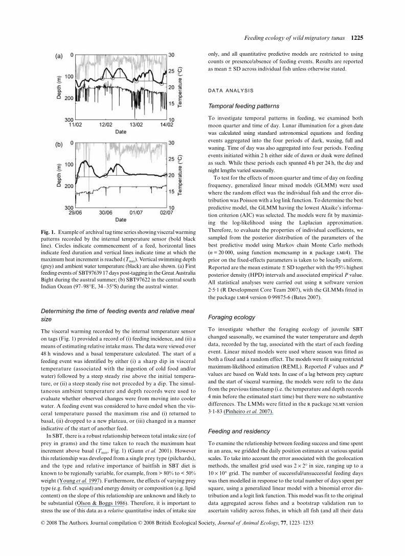
The visceral warming recorded by the internal temperature sensoron tags (Fig. 1) provided a record of (i) feeding incidence, and (ii) ameans of estimating relative intake mass. The data were viewed over48 h windows and a basal temperature calculated. The start of afeeding event was identified by either (i) a sharp dip in visceraltemperature (associated with the ingestion of cold food and/orwater) followed by a steep steady rise above the initial tempera-ture, or (ii) a steep steady rise not preceded by a dip. The simul-taneous ambient temperature and depth records were used toevaluate whether observed changes were from moving into coolerwater. A feeding event was considered to have ended when the vis-ceral temperature passed the maximum rise and (i) returned tobasal, (ii) dropped to a new plateau, or (iii) changed in a mannerindicative of the start of another feed.

In SBT, there is a robust relationship between total intake size (ofprey in grams) and the time taken to reach the maximum heatincrement above basal (

T

max

, Fig. 1) (Gunn

et al.

2001). Howeverthis relationship was developed from a single prey type (pilchards),and the type and relative importance of baitfish in SBT diet isknown to be regionally variable, for example, from > 80% to < 50%weight (Young

et al.

1997). Furthermore, the effects of varying preytype (e.g. fish cf. squid) and energy density or composition (e.g. lipidcontent) on the slope of this relationship are unknown and likely tobe substantial (Olson & Boggs 1986). Therefore, it is important tostress the use of this data as a

relative

quantitative index of intake size

only, and all quantitative predictive models are restricted to usingcounts or presence/absence of feeding events. Results are reportedas mean ± SD across individual fish unless otherwise stated.

DATA

ANALYSIS

Temporal feeding patterns

To investigate temporal patterns in feeding, we examined bothmoon quarter and time of day. Lunar illumination for a given datewas calculated using standard astronomical equations and feedingevents aggregated into the four periods of dark, waxing, full andwaning. Time of day was also aggregated into four periods. Feedingevents initiated within 2 h either side of dawn or dusk were definedas such. While these periods each spanned 4 h per 24 h, the day andnight lengths varied seasonally.

To test for the effects of moon quarter and time of day on feedingfrequency, generalized linear mixed models (GLMM) were usedwhere the random effect was the individual fish and the error dis-tribution was Poisson with a log link function. To determine the bestpredictive model, the GLMM having the lowest Akaike’s informa-tion criterion (AIC) was selected. The models were fit by maximiz-ing the log-likelihood using the Laplacian approximation.Therefore, to evaluate the properties of individual coefficients, wesampled from the posterior distribution of the parameters of thebest predictive model using Markov chain Monte Carlo methods(

n

= 20 000, using function mcmcsamp in

r

package

lme

4). Theprior on the fixed-effects parameters is taken to be locally uniform.Reported are the mean estimate ± SD together with the 95% highestposterior density (HPD) intervals and associated empirical

P

value.All statistical analyses were carried out using

r

software version2·5·1 (R Development Core Team 2007), with the GLMMs fitted inthe package

lme

4 version 0·99875-6 (Bates 2007).

Foraging ecology

To investigate whether the foraging ecology of juvenile SBTchanged seasonally, we examined the water temperature and depthdata, recorded by the tag, associated with the start of each feedingevent. Linear mixed models were used where season was fitted asboth a fixed and a random effect. The models were fit using restrictedmaximum-likelihood estimation (REML). Reported

F

values and

P

values are based on Wald tests. In case of a lag between prey captureand the start of visceral warming, the models were refit to the datafrom the previous timestamp (i.e. the temperature and depth records4 min before the estimated start time) but there were no substantivedifferences. The LMMs were fitted in the

r

package

nlme

version3·1-83 (Pinheiro

et al.

2007).

Feeding and residency

To examine the relationship between feeding success and time spentin an area, we gridded the daily position estimates at various spatialscales. To take into account the error associated with the geolocationmethods, the smallest grid used was 2

×

2

°

in size, ranging up to a10

×

10

°

grid. The number of successful/unsuccessful feeding dayswas then modelled in response to the total number of days spent persquare, using a generalized linear model with a binomial error dis-tribution and a logit link function. This model was fit to the originaldata aggregated across fishes and a bootstrap validation run toascertain validity across fishes, in which all fish (and all their data

Fig. 1. Example of archival tag time series showing visceral warmingpatterns recorded by the internal temperature sensor (bold blackline). Circles indicate commencement of a feed, horizontal linesindicate feed duration and vertical lines indicate time at which themaximum heat increment is reached (Tmax). Vertical swimming depth(grey) and ambient water temperature (black) are also shown. (a) Firstfeeding events of SBT97639 17 days post-tagging in the Great AustraliaBight during the austral summer; (b) SBT97622 in the central southIndian Ocean (97–98°E, 34–35°S) during the austral winter.

1226

S. Bestley

et al

.

© 2008 The Authors. Journal compilation © 2008 British Ecological Society,

Journal of Animal Ecology

,

77

, 1223–1233

points) were sampled with replacement and the model refit(

n

= 10 000). To investigate further the pattern for individual fish,we examined GLMMs with a binomial error distribution. Datafrom squares centred within the GAB coastal summer residencyarea bounded by the coordinates (127·5

°

E, 29

°

S), (127·5

°

E, 34

°

S),(140

°

E, 34

°

S), (140

°

E, 42·5

°

S) were excluded from this analysis. Fishwith data available only for the outward migration leg from theGAB, that is, without any oceanic residencies, due to early tag fail-ure (

n

= 3) or recapture (

n

= 1), were also excluded.

Results

A total of 6221 days of data were collected from the 19 fish,with individual time series spanning 141–496 days (Table 1).Individuals recommenced feeding between 5 and 38 daysafter tagging (mean ± SD: 19 ± 10 days). These post-releasefasting periods were excluded from all analyses. Feedingevents (

n

= 5194) were subsequently identified on 76·3 ± 5·8%of days (range: 63·5–84·9%), for an overall feeding rate of0·89 ± 0·08 feeding events per day per individual (range:0·76–1·16). On feeding days, the feeding rate was 1·17 ± 0·09(range: 1·05–1·48). The estimated daily intake was 0·75 ±0·05 kg (range: 0·67–0·85 kg) and the mean feed size was 0·85 ±0·09 kg (range: 0·63–1·03). The mean duration of the visceraltemperature signature was 18·5 ± 1·4 h (range: 14·4–20·9).The minimum interval recorded between feeding events was40 min; however, there was a distinct diurnal cycle with themedian ranging between 18·7–24·1 h. There was considerablevariation in the maximum between-feed interval, with indi-

viduals recording periods of up to 3·9–24·4 days withoutfeeding (mean ± SD: 11·4 ± 6·5).

TEMPORAL

PATTERNS

IN

FEEDING

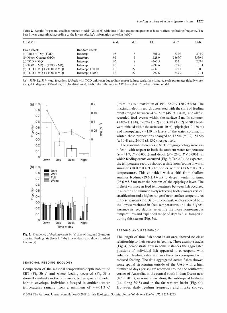
The number of feeding events varied strongly with time of theday (GLMM, all

|

z

|

> 24,

P

< 0·0001; Table 2) with the high-est number of feeding events (58·2 ± 8·0%) and feeding rate(0·16 ± 0·03 feeds h

–1

) occurring near dawn (Fig. 2a). Somefeeding activity occurred during the day (26·0 ± 6·4%) butrarely at night (5·7 ± 1·3%, Fig. 2a). Moon quarter was not asignificant independent factor influencing the number offeeding events (GLMM, all

|

z

|

< 1,

P

> 0·3), however themoon quarter-time of day interaction was significant (Table 2).Night feeds during the full moon quarter were predicted to bemore likely by a factor of 10·7 (± 1·3, 95% highest posteriordensity (HPD) = 6·2–19·6,

P

< 0·0001) relative to the darkmoon, and by a factor of 5·6 (± 1·4, 95% HPD = 3·1–10·2,

P

< 0·0001) and 3·3 (± 1·4 SE, 95% HPD = 1·8–6·3,

P

= 0·0001)during the waning and waxing quarters, respectively (Fig. 2b).A weaker effect of the full moon was a small decline in dawnfeeding (by a factor of 0·8 ± 1·1, 95% HPD = 0·7–0·9,

P

= 0·0001) and increase in day and dusk feeding (by a factorof 1·5 ± 1·1, 95% HPD = 1·2–1·8,

P

< 0·0001, and 1·6 ± 1·1,95% HPD = 1·3–2·0,

P

= 0·0001 respectively). The best modelexplicitly included a random effect for time of day withinfishes, due to small variations in relative feed incidencebetween day and dusk.

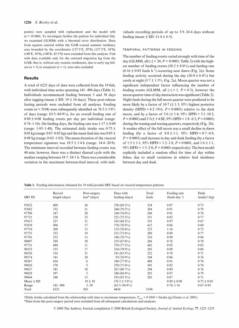
Table 1. Feeding information obtained for 19 wild juvenile SBT based on visceral temperature patterns

SBT IDRecord length (days)

Post-surgery fast* (days)

Days with feeding (days)

Total feeds

Feeding rate (feeds day–1)

Daily intake† (kg)

97622 409 36 258 (69·2%) 324 0·87 0·7597682 332 21 244 (78·5%) 284 0·91 0·7997708 247 20 168 (74·0%) 206 0·91 0·7897721 338 32 221 (72·2%) 251 0·82 0·7797615 227 31 165 (84·2%) 191 0·97 0·6797639 496 17 378 (78·9%) 412 0·86 0·6997718 209 15 152 (78·4%) 225 1·16 0·7397733 332 19 231 (73·8%) 280 0·89 0·7797741 252 13 188 (78·7%) 216 0·90 0·8498007 389 38 235 (67·0%) 266 0·76 0·7897731 490 11 370 (77·2%) 442 0·92 0·8598553 335 17 254 (79·9%) 283 0·89 0·8098556 316 31 181 (63·5%) 222 0·78 0·7198574 141 20 93 (76·9%) 104 0·86 0·7699267 454 6 349 (77·9%) 408 0·91 0·7099626 370 5 259 (71·0%) 301 0·82 0·7099627 341 10 267 (80·7%) 294 0·89 0·7699629 297 5 248 (84·9%) 283 0·97 0·7999664 246 15 193 (83·5%) 202 0·87 0·71Mean ± SD 19 ± 10 (76·3 ± 5·8%) 0·89 ± 0·08 0·75 ± 0·05Range 141–496 5–38 (63·5–84·9%) 0·76–1·16 0·67–0·85Total 6221 362 4454 5194

†Daily intake calculated from the relationship with time to maximum temperature, Tmax = 0·5845 * Intake (g) (Gunn et al, 2001).*Data from this post-surgery period were excluded from all subsequent calculations and analyses.

Feeding ecology of wild migratory tunas

1227

© 2008 The Authors. Journal compilation © 2008 British Ecological Society, Journal of Animal Ecology, 77, 1223–1233

SEASONAL FEEDING ECOLOGY

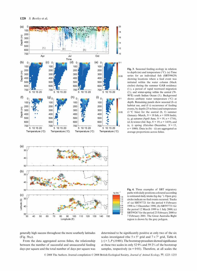
Comparison of the seasonal temperature–depth habitat ofSBT (Fig. 3b–e) and where feeding occurred (Fig. 3f–i)showed similarity in the core areas, but in general a widerhabitat envelope. Individuals foraged in ambient watertemperatures ranging from a minimum of 4·9–11·3 °C

(9·0 ± 1·4) to a maximum of 19·3–22·9 °C (20·9 ± 0·8). Themaximum depth records associated with the start of feedingevents ranged between 247–672 m (460 ± 134 m), and all fishrecorded feed events within the surface 2 m. In summer,41·8% (± 11·8), 55·2% (± 9·2) and 3·0% (± 6·2) of SBT feedswere initiated within the surface (0–10 m), epipelagic (10–150 m)and mesopelagic (> 150 m) layers of the water column. Inwinter, these proportions changed to 17·5% (± 7·9), 58·5%(± 10·4) and 24·0% (± 13·2), respectively.

The seasonal differences in SBT foraging ecology were sig-nificant with respect to both the ambient water temperature(F = 41·7, P < 0·0001) and depth (F = 26·0, P < 0·0001) inwhich feeding events occurred (Fig. 3; Table 3). As expected,the temperature records showed a shift from feeding in warmsummer (18·0 ± 0·4 °C) to cooler winter (13·6 ± 0·2 °C)temperatures. This coincided with a shift from shallowsummer feeding (29·6 ± 4·6 m) to deeper winter foraging(96·6 ± 8·5 m) near the bottom of the epipelagic layer. Thehighest variance in feed temperatures between fish occurredin autumn and summer, likely reflecting both stronger verticalstratification and a higher range of near-surface temperaturesin these seasons (Fig. 3a,b). In contrast, winter showed boththe lowest variance in feed temperatures and the highestvariance in feed depths, reflecting the more homogeneoustemperatures and expanded range of depths SBT foraged induring this season (Fig. 3c).

FEEDING AND RESIDENCY

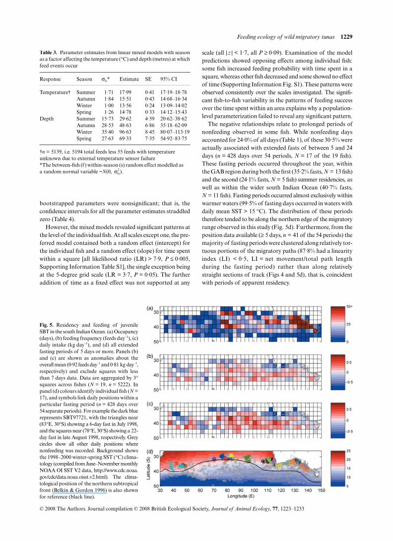
The length of time fish spent in an area showed no clearrelationship to their success in feeding. Three example tracks(Fig. 4) demonstrate how in some instances the aggregatedpositions of individual fish appeared to correspond withenhanced feeding rates, and in others to correspond withreduced feeding. The data aggregated across fishes showedsome spatial structuring outside of the GAB with a highnumber of days per square recorded around the south-westcorner of Australia, in the central south Indian Ocean near(40°S, 80°E), in some areas along the subtropical latitudes(i.e. along 30°S) and in the far western basin (Fig. 5a).However, daily feeding frequency and intake showed

Table 2. Results for generalized linear mixed models (GLMM) with time of day and moon quarter as factors affecting feeding frequency. Thebest fit was determined according to the lowest Akaike’s information criterion (AIC)

GLMM† Scale d.f. LL AIC ΔAIC

Fixed effects Random effects(a) Time of Day (TOD) Intercept 1·5 5 –361·2 732·3 204·2(b) Moon Quarter (MQ) Intercept 3·5 5 –1928·9 3867·7 3339·6(c) TOD + MQ Intercept 1·5 8 –360·5 737 208·9(d) TOD + MQ + (TOD × MQ) Intercept 1·3 17 –297·6 629·2 101·1(e) TOD + MQ + (TOD × MQ) Intercept + TOD 1·0 27 –237·1 528·1 0(f) TOD + MQ + (TOD × MQ) Intercept + MQ 1·3 27 –297·6 649·2 121·1

†n = 5179, i.e. 5194 total feeds less 15 feeds with TOD unknown due to light sensor failure; scale, the estimated scale parameter (ideally close to 1); d.f., degrees of freedom; LL, log-likelihood; ΔAIC, the difference in AIC from that of the best-fitting model.

Fig. 2. Frequency of feeding events by (a) time of day, and (b) moonquarter. Feeding rate (feeds hr–1) by time of day is also shown (dashedline) in (a).

1228 S. Bestley et al.

© 2008 The Authors. Journal compilation © 2008 British Ecological Society, Journal of Animal Ecology, 77, 1223–1233

generally high success throughout the more southerly latitudes(Fig. 5b,c).

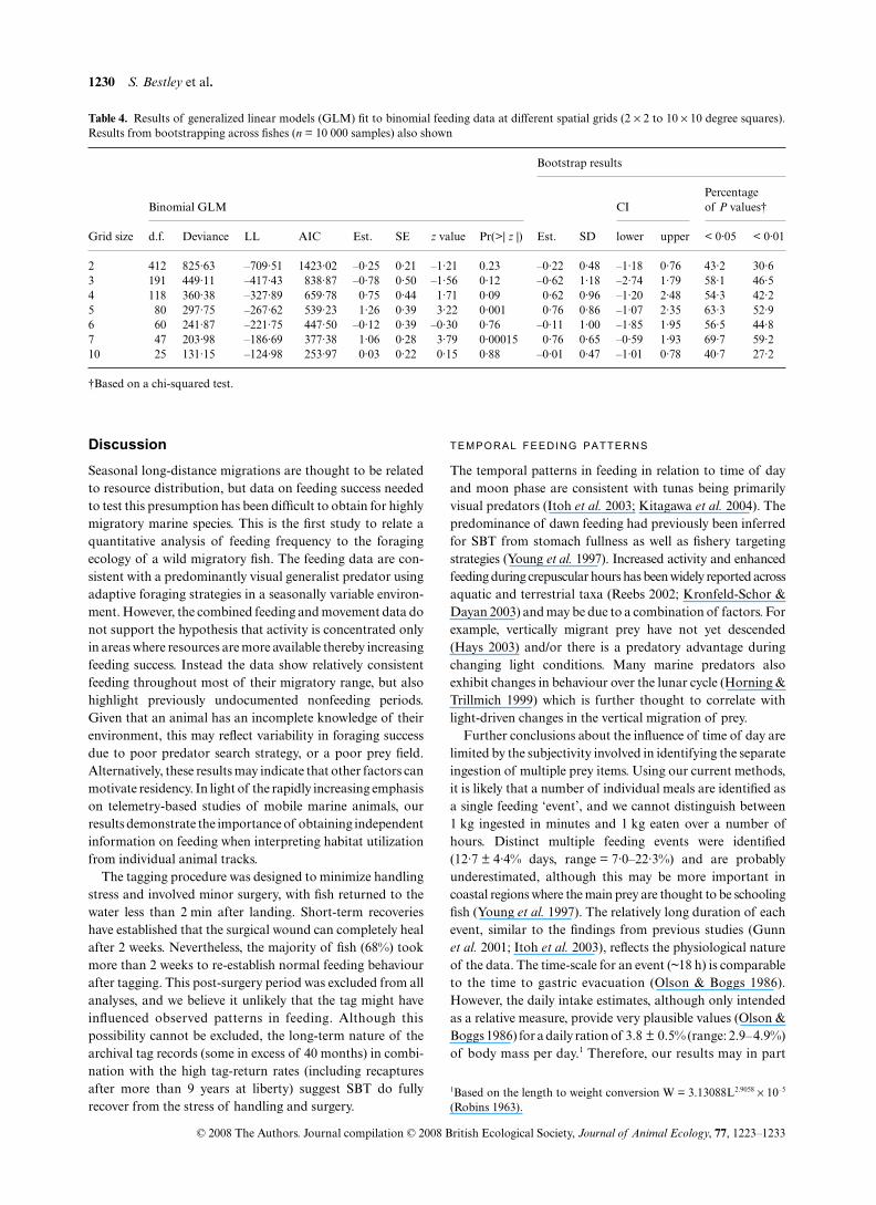
From the data aggregated across fishes, the relationshipbetween the number of successful and unsuccessful feedingdays per square and the total number of days per square was

determined to be significantly positive at only two of the sixscales investigated (the 5 × 5° grid and 7 × 7° grid, Table 4;| z | > 3, P ≤ 0·001). The bootstrap procedure showed significanceat these two scales in only 52·9% and 59·2% of the bootstrapsamples, respectively (α = 0·01). Therefore, at all scales the

Fig. 3. Seasonal feeding ecology in relationto depth (m) and temperature (°C). (a) Timeseries for an individual fish (SBT99629)showing locations where a feed event wasinitiated within the water column (blackcircles) during the summer GAB residency(1.), a period of rapid westward migration(2.), and winter-spring within the central (70–90°E) south Indian Ocean (3.). Backgroundshows ambient water temperature (°C) atdepth. Remaining panels show seasonal (b–e)habitat use, and (f–i) occurrence of feedingevents, by depth (25 m bins) and temperature(1 °C bins) for the austral (b, f ) summer(January–March, N = 18 fish, n = 1058 feeds),(c, g) autumn (April–June, N = 19, n = 1716),(d, h) winter (Jul–Sep, N = 19, n = 1419), and(e, i) spring (October–December, N = 15,n = 1000). Data in (b) – (i) are aggregated asaverage proportions across fishes.

Fig. 4. Three examples of SBT migratorypaths with daily positions coloured accordingto estimated daily intake (kg day–1). Open greycircles indicate no feed events occurred. Tracksof (a) SBT97721 for the period 4 February1998 to 5 December 1998; (b) SBT97731 forthe period 12 March 1999 to 1 July 2000; (c)SBT99267 for the period 23 February 2000 to7 February 2001. The Great Australia Bightregion is shown by the grey polygon.

Feeding ecology of wild migratory tunas 1229

© 2008 The Authors. Journal compilation © 2008 British Ecological Society, Journal of Animal Ecology, 77, 1223–1233

bootstrapped parameters were nonsignificant; that is, theconfidence intervals for all the parameter estimates straddledzero (Table 4).

However, the mixed models revealed significant patterns atthe level of the individual fish. At all scales except one, the pre-ferred model contained both a random effect (intercept) forthe individual fish and a random effect (slope) for time spentwithin a square [all likelihood ratio (LR) > 7·9, P ≤ 0·005,Supporting Information Table S1], the single exception beingat the 5-degree grid scale (LR = 3·7, P = 0·05). The furtheraddition of time as a fixed effect was not supported at any

scale (all | z | < 1·7, all P ≥ 0·09). Examination of the modelpredictions showed opposing effects among individual fish:some fish increased feeding probability with time spent in asquare, whereas other fish decreased and some showed no effectof time (Supporting Information Fig. S1). These patterns wereobserved consistently over the scales investigated. The signifi-cant fish-to-fish variability in the patterns of feeding successover the time spent within an area explains why a population-level parameterization failed to reveal any significant pattern.

The negative relationships relate to prolonged periods ofnonfeeding observed in some fish. While nonfeeding daysaccounted for 24·0% of all days (Table 1), of these 30·5% wereactually associated with extended fasts of between 5 and 24days (n = 428 days over 54 periods, N = 17 of the 19 fish).These fasting periods occurred throughout the year, withinthe GAB region during both the first (35·2% fasts, N = 13 fish)and the second (24·1% fasts, N = 5 fish) summer residencies, aswell as within the wider south Indian Ocean (40·7% fasts,N = 11 fish). Fasting periods occurred almost exclusively withinwarmer waters (99·5% of fasting days occurred in waters withdaily mean SST > 15 °C). The distribution of these periodstherefore tended to be along the northern edge of the migratoryrange observed in this study (Fig. 5d). Furthermore, from theposition data available (≥ 5 days, n = 41 of the 54 periods) themajority of fasting periods were clustered along relatively tor-tuous portions of the migratory paths (87·8% had a linearityindex (LI) < 0·5, LI = net movement/total path lengthduring the fasting period) rather than along relativelystraight sections of track (Figs 4 and 5d), that is, coincidentwith periods of apparent residency.

Table 3. Parameter estimates from linear mixed models with seasonas a factor affecting the temperature (°C) and depth (metres) at whichfeed events occur

Response Season σfs* Estimate SE 95% CI

Temperature† Summer 1·71 17·99 0·41 17·19–18·78Autumn 1·84 15·51 0·43 14·68–16·34Winter 1·00 13·56 0·24 13·09–14·02Spring 1·26 14·78 0·33 14·12–15·43

Depth Summer 15·73 29·62 4·59 20·62–38·62Autumn 28·53 48·63 6·86 35·18–62·09Winter 35·40 96·63 8·45 80·07–113·19Spring 27·63 69·33 7·35 54·92–83·75

†n = 5139, i.e. 5194 total feeds less 55 feeds with temperature unknown due to external temperature sensor failure*The between-fish (f) within-season (s) random effect modelled as a random normal variable ~N(0, ).σfs

2

Fig. 5. Residency and feeding of juvenileSBT in the south Indian Ocean. (a) Occupancy(days), (b) feeding frequency (feeds day–1), (c)daily intake (kg day–1), and (d) all extendedfasting periods of 5 days or more. Panels (b)and (c) are shown as anomalies about theoverall mean (0·92 feeds day–1 and 0·81 kg day–1,respectively) and exclude squares with lessthan 7 days data. Data are aggregated by 3°squares across fishes (N = 19, n = 5222). Inpanel (d) colours identify individual fish (N =17), and symbols link daily positions within aparticular fasting period (n = 428 days over54 separate periods). For example the dark bluerepresents SBT97721, with the triangles near(83°E, 30°S) showing a 6-day fast in July 1998,and the squares near (78°E, 30°S) showing a 22-day fast in late August 1998, respectively. Greycircles show all other daily positions wherenonfeeding was recorded. Background showsthe 1998–2000 winter-spring SST (°C) clima-tology (compiled from June–November monthlyNOAA OI SST V2 data, http://www.cdc.noaa.gov/cdc/data.noaa.oisst.v2.html). The clima-tological position of the northern subtropicalfront (Belkin & Gordon 1996) is also shownfor reference (black line).

1230 S. Bestley et al.

© 2008 The Authors. Journal compilation © 2008 British Ecological Society, Journal of Animal Ecology, 77, 1223–1233

Discussion

Seasonal long-distance migrations are thought to be relatedto resource distribution, but data on feeding success neededto test this presumption has been difficult to obtain for highlymigratory marine species. This is the first study to relate aquantitative analysis of feeding frequency to the foragingecology of a wild migratory fish. The feeding data are con-sistent with a predominantly visual generalist predator usingadaptive foraging strategies in a seasonally variable environ-ment. However, the combined feeding and movement data donot support the hypothesis that activity is concentrated onlyin areas where resources are more available thereby increasingfeeding success. Instead the data show relatively consistentfeeding throughout most of their migratory range, but alsohighlight previously undocumented nonfeeding periods.Given that an animal has an incomplete knowledge of theirenvironment, this may reflect variability in foraging successdue to poor predator search strategy, or a poor prey field.Alternatively, these results may indicate that other factors canmotivate residency. In light of the rapidly increasing emphasison telemetry-based studies of mobile marine animals, ourresults demonstrate the importance of obtaining independentinformation on feeding when interpreting habitat utilizationfrom individual animal tracks.

The tagging procedure was designed to minimize handlingstress and involved minor surgery, with fish returned to thewater less than 2 min after landing. Short-term recoverieshave established that the surgical wound can completely healafter 2 weeks. Nevertheless, the majority of fish (68%) tookmore than 2 weeks to re-establish normal feeding behaviourafter tagging. This post-surgery period was excluded from allanalyses, and we believe it unlikely that the tag might haveinfluenced observed patterns in feeding. Although thispossibility cannot be excluded, the long-term nature of thearchival tag records (some in excess of 40 months) in combi-nation with the high tag-return rates (including recapturesafter more than 9 years at liberty) suggest SBT do fullyrecover from the stress of handling and surgery.

TEMPORAL FEEDING PATTERNS

The temporal patterns in feeding in relation to time of dayand moon phase are consistent with tunas being primarilyvisual predators (Itoh et al. 2003; Kitagawa et al. 2004). Thepredominance of dawn feeding had previously been inferredfor SBT from stomach fullness as well as fishery targetingstrategies (Young et al. 1997). Increased activity and enhancedfeeding during crepuscular hours has been widely reported acrossaquatic and terrestrial taxa (Reebs 2002; Kronfeld-Schor &Dayan 2003) and may be due to a combination of factors. Forexample, vertically migrant prey have not yet descended(Hays 2003) and/or there is a predatory advantage duringchanging light conditions. Many marine predators alsoexhibit changes in behaviour over the lunar cycle (Horning &Trillmich 1999) which is further thought to correlate withlight-driven changes in the vertical migration of prey.

Further conclusions about the influence of time of day arelimited by the subjectivity involved in identifying the separateingestion of multiple prey items. Using our current methods,it is likely that a number of individual meals are identified asa single feeding ‘event’, and we cannot distinguish between1 kg ingested in minutes and 1 kg eaten over a number ofhours. Distinct multiple feeding events were identified(12·7 ± 4·4% days, range = 7·0–22·3%) and are probablyunderestimated, although this may be more important incoastal regions where the main prey are thought to be schoolingfish (Young et al. 1997). The relatively long duration of eachevent, similar to the findings from previous studies (Gunnet al. 2001; Itoh et al. 2003), reflects the physiological natureof the data. The time-scale for an event (~18 h) is comparableto the time to gastric evacuation (Olson & Boggs 1986).However, the daily intake estimates, although only intendedas a relative measure, provide very plausible values (Olson &Boggs 1986) for a daily ration of 3.8 ± 0.5% (range: 2.9–4.9%)of body mass per day.1 Therefore, our results may in part

Table 4. Results of generalized linear models (GLM) fit to binomial feeding data at different spatial grids (2 × 2 to 10 × 10 degree squares).Results from bootstrapping across fishes (n = 10 000 samples) also shown

Grid size

Binomial GLM

Bootstrap results

CIPercentage of P values†

d.f. Deviance LL AIC Est. SE z value Pr(>| z |) Est. SD lower upper < 0·05 < 0·01

2 412 825·63 –709·51 1423·02 –0·25 0·21 –1·21 0.23 –0·22 0·48 –1·18 0·76 43·2 30·63 191 449·11 –417·43 838·87 –0·78 0·50 –1·56 0·12 –0·62 1·18 –2·74 1·79 58·1 46·54 118 360·38 –327·89 659·78 0·75 0·44 1·71 0·09 0·62 0·96 –1·20 2·48 54·3 42·25 80 297·75 –267·62 539·23 1·26 0·39 3·22 0·001 0·76 0·86 –1·07 2·35 63·3 52·96 60 241·87 –221·75 447·50 –0·12 0·39 –0·30 0·76 –0·11 1·00 –1·85 1·95 56·5 44·87 47 203·98 –186·69 377·38 1·06 0·28 3·79 0·00015 0·76 0·65 –0·59 1·93 69·7 59·210 25 131·15 –124·98 253·97 0·03 0·22 0·15 0·88 –0·01 0·47 –1·01 0·78 40·7 27·2

†Based on a chi-squared test.

1Based on the length to weight conversion W = 3.13088L2.9058 × 10–5

(Robins 1963).

Feeding ecology of wild migratory tunas 1231

© 2008 The Authors. Journal compilation © 2008 British Ecological Society, Journal of Animal Ecology, 77, 1223–1233

represent the efficiency of a predator aiming to fill its stomachonce per day, and feeding rapidly to satiation when theopportunity arises.

SEASONAL FORAGING ECOLOGY

Our findings show juvenile SBT predominantly exploit theepipelagic ocean, with some feeding also occurring within themesopelagic layer particularly during winter. The deepestrecorded feeding event (672 m) also provides evidence thatSBT occasionally forage at very low light levels, consistentwith previous reports of deep-sea crustaceans and bottom-dwelling fish in their diet. A deeper winter vertical distribution,and by inference feeding depth, has been previously reportedfor other tunas (Thunnus orientalis; Kitagawa et al. 2004) andpredatory fish (Oncorhynchus tshawytscha; Hinke et al. 2005).Studies of marine predators in the southern oceans such aspenguins and seals have also reported deeper diving patterns,increased diving effort, expanded foraging ranges and anincreased diversity of prey items during winter (Aptenodytes

patagonicus; Cherel, Ridoux & Rodhouse 1996; Arctocephalus

tropicalis; Beauplet et al. 2004; Eudyptes chrysolophus; Greenet al. 2005). Such behavioural flexibility, as observed across avariety of top predators, has widely been interpreted as aresponse to seasonally reduced epipelagic prey availabilityand density, ensuring broader diets and higher feeding rates.

L INKING FEEDING AND RESIDENCY

Increasingly, quantitative analyses aimed at elucidatingforaging strategies are being applied to high-precisionmovement tracks such as obtained via global positioning systemcollars (Morales et al. 2004). However, the large errorsassociated with geolocation methods, and to a lesser extentArgos satellite estimates, present substantial limitations tothe application of such track-based analytical methods(Bradshaw, Sims & Hays 2007). The geographical grid scalesexamined in this study, although somewhat of an artificialimposition, were selected to cover an appropriate range givenboth the coarse resolution of the data and the spatial scales ofthe movements being studied. The range also encompassedscales previously identified as characteristic of mesoscaleforaging patches for other top predators operating oversimilar spatial scales, although shorter time-scales (Fauchald& Tveraa 2006).

Our analysis found time spent within an area had no clearrelationship with feeding success. Most interestingly, this wasprimarily a result of the high degree of individual variationwith both positive and negative trends observed betweenindividuals. Importantly, these patterns were observedconsistently across all the spatial scales examined. This findingprovides strong evidence against the interpretation of high-use areas for migratory species, commonly determined fromonly horizontal and/or vertical movement data in the absenceof any independent information on feeding activity, assuccessful feeding grounds (Robinson et al. 2007). Thisstrengthens previous findings from studies using indirect

measures such as body condition (Bailleul et al. 2007) andmass gain (Bradshaw et al. 2004) which found equivocal or noevidence for a relationship between foraging success andspatial usage of areas. Explanations for the observed variation intrends can be (i) time spent within an area is more likely to bea measure of searching activity rather than a direct proxy forforaging success, given that predators have imperfect knowledgeof their environment; and (ii) predators do not necessarilyfeed all the time, and may spend time within areas for alternativereasons.

Although animal movements may be driven by resourcedistribution, superimposed on this is the fact that they mayhave incomplete knowledge of their environment, particularly inheterogeneous marine environments. At very broad geographicaland seasonal scales, predators may have an awareness of preydistribution (Bradshaw et al. 2004; Houghton et al. 2006),and at fine-scales foraging is likely to be dominated by proximalsensory clues (Sims & Quayle 1998). However, the mesoscalesearch strategies by which animals locate prey remains a pivotalproblem in ecology. To examine whether animals use optimalsearch strategies, recent studies have used empirical data onboth horizontal and vertical movements (Edwards et al. 2007;Sims et al. 2008), as well as simulations (Sims et al. 2006). Ourfinding that juvenile SBT did not consistently spend longestwhere their feeding success was highest may reflect that asjuveniles, some individuals have poor search strategies (Simset al. 2006); however, no information on adult foraging iscurrently available to determine if this is a specific juvenilebehaviour. Since our study examined same-age individualswithin a narrow size range, therefore presumably similarlevels of foraging experience and skill, the high variability inpatterns of feeding between individuals are not expected to berelated to age or size. Yet as unsexed juveniles, it was not pos-sible to determine whether the differences were sex-related.

The variable patterns of feeding success may reflect realdifferences in the availability of prey or the prey type targetedby individuals. High individual variability in feeding behaviour,not specific to juvenile cases, has been reported in many othertop predators including seals (Halichoerus grypus; Austinet al. 2006), albatross (Diomedea exulans; Weimerskirch et al.

1997) and penguins (A. patagonicus; Putz & Bost 1994), andgenerally attributed to the patchy and unpredictable preydistribution. It is also a possibility that the high spatial overlap inthe locations of poor feeding success are indicative of arelatively poor season(s) within a region of usually predictablyhigh forage (Bradshaw et al. 2004). Future studies should revealif (i) SBT do show fidelity to particular regions; and (ii) theidentified areas of low feeding success are consistent orvariable between years.

The second explanation for the observed variation infeeding trends is that large predators do not necessarily feedall the time, and may spend time in particular areas foralternative reasons. Particularly in coastal waters, where SBTexhibit strong schooling behaviour, movements may be drivenby social factors rather than individual-based decision-making (Gunn & Block 2001). In an oceanic context, associationwith floating objects and/or topographic structures has been

1232 S. Bestley et al.

© 2008 The Authors. Journal compilation © 2008 British Ecological Society, Journal of Animal Ecology, 77, 1223–1233

proposed as a behaviour that increases the encounter ratebetween isolated migratory fishes (Freon & Dagorn 2000).Alternatively, particular topographic features may be importantfor other reasons such as resting or for navigational reference(Castro, Santiago & Santana-Ortega 2001). Movements mayalso be related to predator avoidance, which is often ignoredfor large species but has been demonstrated in bottlenosedolphins (Tursiops aduncus) and green turtles (Chelonia mydas)where there are high abundances of sharks (Heithaus & Dill2006; Heithaus et al. 2007). Finally, it has been suggested thatwhen tunas forage within frontal zones, the warm side of frontsmay be used as a thermal refuge, enabling them to feed in coldwaters while minimizing the cost of staying warm (Gunn &Young 1999; Kitagawa et al. 2004). Thermal conditions areknown to play a driving role in the large-scale movementsof a range of marine predators including turtles, fish andmammals (McMahon & Hays 2006; Neat & Righton 2007). Inour study, the prevalence of nonfeeding periods in warmwaters (Fig. 5d) provides some evidence that resting periodsmay occur within thermal refuges over longer time-scales (ofdays to weeks) in the south Indian Ocean.

In summary, we have shown the value of integrating directinformation on feeding when interpreting habitat utilizationfrom individual animal tracks. Our findings do not show astraightforward relationship between feeding and residency.Current efforts to develop novel methods for determiningfeeding activity on a wide range of marine species will continueto advance our understanding of foraging ecology and thecritical linkages between animal behaviour, movement,environment and energetics.

Acknowledgements

Tag deployments were funded under the collaborative SBT RecruitmentMonitoring Program by the Japan Marine Fishery Resources Research Center(JAMARC), the Commonwealth Scientific and Industrial Research Organization(CSIRO), and the Australian Fisheries Management Authority (AFMA). Allprocedures were approved by the Australian Primary Industries and WaterAnimal Ethics Committee. We thank the Australian purse-seine industry, aswell as the Australian and international long-line fishermen, for their cooper-ation in returning tags. We also acknowledge the ongoing contribution of manyCSIRO staff and particularly thank K. Tattersall for the feed identificationwork. Thanks to M. Bravington and S. Foster for statistical advice. This studywas supported by a joint CSIRO-UTAS QMS scholarship and a CSIROPostgraduate Award to S.B. C. Davies, G. Hays and two anonymous reviewersprovided constructive comments on the manuscript that were greatly appreciated.

References

Alerstam, T., Hedenstrom, A. & Akesson, S. (2003) Long-distance migration:evolution and determinants. Oikos, 103, 247–260.

Austin, D., Bowen, W.D., McMillan, J.I. & Boness, D.J. (2006) Stomachtemperature telemetry reveals temporal patterns of foraging success infree-ranging marine mammal. Journal of Animal Ecology, 75, 408–420.

Bailey, H. & Thompson, P. (2006) Quantitative analysis of bottlenose dolphinmovement patterns and their relationship with foraging. Journal of Animal

Ecology, 75, 456–465.Bailey, H., Shillinger, G., Palacios, D., Bograd, S., Spotila, J., Paladino, F. & Block, B.

(2008) Identifying and comparing phases of movement by leatherbackturtles using state-space models. Journal of Experimental Marine Biology

and Ecology, 356, 128–135.Bailleul, F., Charrassin, J.B., Monestiez, P., Roquet, F., Biuw, M. & Guinet, C.

(2007) Successful foraging zones of southern elephant seals from the

Kerguelen Islands in relation to oceanographic conditions. Philosophical

Transactions of the Royal Society B-Biological Sciences, 362, 2169–2181.Baker, R.R. (1978) The Evolutionary Ecology of Animal Migration. Hodder

and Stoughton, London, UK.Bates, D. (2007) LME4: Linear Mixed-Effects Models Using S4 Classes. R package

version 0·99875-6. http://www.stats.bris.ac.uk/R.Beauplet, G., Dubroca, L., Guinet, C., Cherel, Y., Dabin, W., Gagne, C. &

Hindell, M. (2004) Foraging ecology of subantarctic fur seals Arctocephalus

tropicalis breeding on Amsterdam Island: seasonal changes in relation tomaternal characteristics and pup growth. Marine Ecology Progress Series,273, 211–225.

Belkin, I.M. & Gordon, A.L. (1996) Southern Ocean fronts from the Greenwichmeridian to Tasmania. Journal of Geophysical Research, 101, 3675–3696.

Boyd, I.L. & Croxall, J.P. (1996) Dive durations in pinnipeds and seabirds.Canadian Journal of Zoology, 74, 1696–1705.

Bradshaw, C.J.A., Hindell, M.A., Sumner, M.D. & Michael, K.J. (2004)Loyalty pays: potential life history consequences of fidelity to marineforaging regions by southern elephant seals. Animal Behaviour, 68, 1349–1360.

Bradshaw, C.J.A., Sims, D.W. & Hays, G.C. (2007) Measurement error causesscale-dependent threshold erosion of biological signals in animal movementdata. Ecological Applications, 17, 628–638.

Carey, F.G., Kanwisher, J.W. & Stevens, E.D. (1984) Bluefin tuna warm theirviscera during digestion. Journal of Experimental Biology, 109, 1–20.

Castro, J.J., Santiago, J.A. & Santana-Ortega, A.T. (2001) General theory onfish aggregation to floating objects: an alternative to the meeting pointhypothesis. Reviews in Fish Biology and Fisheries, 11, 255–277.

Cherel, Y., Ridoux, V. & Rodhouse, P.G. (1996) Fish and squid in the diet ofking penguin chicks, Aptenodytes patagonicus, during winter at sub-antarctic Crozet Islands. Marine Biology, 126, 559–570.

Edwards, A.M., Phillips, R.A., Watkins, N.W., Freeman, M.P., Murphy, E.J.,Afanasyev, V., Buldyrev, S.V., da Luz, M.G.E., Raposo, E.P., Stanley, H.E.& Viswanathan, G.M. (2007) Revisiting Levy flight search patterns ofwandering albatrosses, bumblebees and deer. Nature, 449, 1044–U5.

Eveson, J.P., Laslett, G.M. & Polacheck, T. (2004) An integrated model forgrowth incorporating tag-recapture, length-frequency, and directaging data. Canadian Journal of Fisheries and Aquatic Sciences, 61, 292–306.

Fauchald, P. & Tveraa, T. (2006) Hierarchical patch dynamics and animalmovement pattern. Oecologia, 149, 383–395.

Fossette, S., Gaspar, P., Handrich, Y., Le Maho, Y. & Georges, J.-Y. (2008) Diveand beak movement patterns in leatherback turtles Dermochelys coriacea

during internesting intervals in French Guiana. Journal of Animal Ecology,77, 236–246.

Freon, P. & Dagorn, L. (2000) Review of fish associative behaviour: towardgeneralisation of the meeting point hypothesis. Reviews in Fish Biology and

Fisheries, 10, 183–207.Gales, R. & Renouf, D. (1993) Detecting and measuring food and water intake

in captive seals using temperature telemetry. Journal of Wildlife Management,57, 514–519.

Green, J.A., Boyd, I.L., Woakes, A.J., Warren, N.L. & Butler, P.J. (2005) Beha-vioural flexibility during year-round foraging in macaroni penguins. Marine

Ecology Progress Series, 296, 183–196.Guinet, C., Dubroca, L., Lea, M.A., Goldsworthy, S., Cherel, Y., Duhamel, G.,

Bonadonna, F. & Donnay, J.-P. (2001) Spatial distribution of foraging infemale Antarctic fur seals Arctocephalus gazella in relation to oceanographicvariables: scale-dependent approach using geographic information systems.Marine Ecology Progress Series, 219, 251–264.

Gunn, J. & Block, B.A. (2001) Advances in acoustic, archival and pop-upsatellite tagging of tunas. Tunas: Physiology, Ecology and Evolution (eds B.A.Block & E.D. Stevens), Vol. 19, pp. 167–224. Academic Press, San Diego CA.

Gunn, J. & Young, J. (1999) Environmental determinants of the movement andmigration of juvenile southern bluefin tuna. Australian Society for Fish Biology

Workshop Proceedings: Fish Movement and Migration (eds D.A. Hancock,D.C. Smith & J.D. Koehn), pp. 123–128. Australian Society for Fish Biology,Bendigo, Australia.

Gunn, J., Hartog, J. & Rough, K. (2001). The relationship between food intakeand visceral warming in southern bluefin tuna (Thunnus maccoyii): can wepredict how much tuna has eaten from archival tag data? Electronic Tagging

and Tracking in Marine Fisheries (eds J.R. Sibert & J.L. Neilson), pp. 109–130. Kluwer Academic Publishers, Dordrecht, The Netherlands.

Hays, G.C. (2003) Review of the adaptive significance and ecosystem consequencesof zooplankton diel vertical migrations. Hydrobiologia, 503, 163–170.

Hays, G.C. (2008) Sea turtles: review of some key recent discoveries andremaining questions. Journal of Experimental Marine Biology and Ecology,356, 1–7.

Feeding ecology of wild migratory tunas 1233

© 2008 The Authors. Journal compilation © 2008 British Ecological Society, Journal of Animal Ecology, 77, 1223–1233

Hays, G.C., Hobson, V.J., Metcalfe, J.D., Righton, D. & Sims, D.W. (2006)Flexible foraging movements of leatherback turtles across the north AtlanticOcean. Ecology, 87, 2647–2656.

Heithaus, M.R. & Dill, L.M. (2006) Does tiger shark predation risk influenceforaging habitat use by bottlenose dolphins at multiple spatial scales? Oikos,114, 257–264.

Heithaus, M.R., Frid, A., Wirsing, A.J., Dill, L.M., Fourqurean, J.W.,Burkholder, D., Thomson, J., & Bejder, L. (2007) State-dependent risk-taking by green sea turtles mediates top-down effects of tiger sharkintimidation in marine ecosystem. Journal of Animal Ecology, 76, 837–844.

Hill, R. (1994). Theory of geolocation by light levels. Elephant Seals: Population

Ecology, Behaviour and Physiology (eds B.J. Le Boeuf & R.M. Laws),pp. 227–236. University of California Press, Berkeley, CA.

Hindell, M.A., Harcourt, R.G., Waas, J.R. & Thompson, D. (2002) Fine-scale,three-dimensional spatial use of diving by lactating female Weddell sealsLeptonychotes weddellii. Marine Ecology Progress Series, 242, 275–284.

Hinke, J.T., Foley, D.G., Wilson, C. & Watters, G.M. (2005) Persistent habitatuse by Chinook salmon Oncorhynchus tshawytscha in the coastal ocean.Marine Ecology Progress Series, 304, 207–220.

Horning, M. & Trillmich, F. (1999) Lunar cycles in diel prey migrations exertstronger effect on the diving of juveniles than adult Galapagos furseals. Proceedings of the Royal Society B: Biological Sciences, 266, 1127–1132.

Houghton, J.D.R., Doyle, T.K., Wilson, M.W., Davenport, J. & Hays, G.C.(2006) Jellyfish aggregations and leatherback turtle foraging patterns intemperate coastal environment. Ecology, 87, 1967–1972.

Itoh, T., Tsuji, S. & Nitta, A. (2003) Swimming depth, ambient water temperaturepreference, and feeding frequency of young Pacific bluefin tuna (Thunnus

orientalis) determined with archival tags. Fishery Bulletin, 101, 535–544.Jonsen, I.D., Flenming, J.M. & Myers, R.A. (2005) Robust state-space modeling

of animal movement data. Ecology, 86, 2874–2880.Kitagawa, T., Kimura, S., Nakata, H. & Yamada, H. (2004) Diving behavior of

immature, feeding Pacific bluefin tuna (Thunnus thynnus orientalis) inrelation to season and area: the East China Sea and the Kuroshio–Oyashiotransition region. Fisheries Oceanography, 13, 161–180.

Kronfeld-Schor, N. & Dayan, T. (2003) Partitioning of time as an ecologicalresource. Annual Review of Ecology, Evolution and Systematics, 34, 153–181.

McMahon, C.R. & Hays, G.C. (2006) Thermal niche, large-scale movementsand implications of climate change for critically endangered marinevertebrate. Global Change Biology, 12, 1330–1338.

Morales, J.M., Haydon, D.T., Frair, J., Holsiner, K.E. & Fryxell, J.M. (2004)Extracting more out of relocation data: building movement models asmixtures of random walks. Ecology, 85, 2436–2445.

Neat, F. & Righton, D. (2007) Warm water occupancy by North Sea cod.Proceedings of the Royal Society B: Biological Sciences, 274, 789–798.

Olson, R.J. & Boggs, C.H. (1986) Apex predation by yellowfin tuna (Thunnus

albacares): independent estimates from gastric evacuation and stomachcontents, bioenergetics, and cesium concentrations. Canadian Journal of

Fisheries and Aquatic Sciences, 43, 1760–1775.Pinheiro, J., Bates, D., DebRoy, S. & Sarkar, D. (2007) NLME: linear and nonlinear

mixed effects models. R package version, 3.1–83. http://www.stats.bris.ac.uk/R/.

Putz, K. & Bost, C.A. (1994) Feeding behavior of free-ranging king penguins(Aptenodytes patagonicus). Ecology, 75, 489–497.

R Development Core Team (2007) R: A Language and Environment for Statis-

tical Computing. R Foundation for Statistical Computing, Vienna, Austria.Available from URL: http://www.R-project.org

Reebs, S.G. (2002) Plasticity of diel and circadian activity rhythms in fishes.Reviews in Fish Biology and Fisheries, 12, 349–371.

Robins, J.P. (1963) Synopsis of biological data on bluefin tuna, Thunnus thynnus

maccoyii (Castelnau) 1872. FAO Fisheries Report, 6, 562–587.Robinson, P.W., Tremblay, Y., Crocker, D.E., Kappes, M.A., Kuhn, C.E.,

Shaffer, S.A., Simmons, S.E. & Costa, D.P. (2007) Comparison of indirectmeasures of feeding behaviour based on ARGOS tracking data. Deep-Sea

Research II, 54, 356–368.Ropert-Coudert, Y. & Wilson, R.P. (2005) Trends and perspectives in animal attached

remote sensing. Frontiers in Ecology and the Environment, 3, 437–444.Shaffer, S.A., Costa, D.P. & Weimerskirch, H. (2001) Behavioural factors

affecting foraging effort of breeding wandering albatrosses. Journal of

Animal Ecology, 70, 864–874.Sims, D., Southall, E., Humphries, N., Hays, G., Bradshaw, C., Pitchford, J.,

James, A., Ahmed, M., Brierley, A., Hindell, M., Morritt, D., Musyl, M.,

Righton, D., Shepard, E., Wearmouth, V., Wilson, R., Witt, M. & Metcalfe, J.(2008) Scaling laws of marine predator search behaviour. Nature, 451,1098–1095.

Sims, D.W. & Quayle, V.A. (1998) Selective foraging behaviour of baskingsharks on zooplankton in small-scale front. Nature, 393, 460–464.

Sims, D.W., Witt, M.J., Richardson, A.J., Southall, E.J. & Metcalfe, J.D. (2006)Encounter success of free-ranging marine predator movements acrossdynamic prey landscape. Proceedings of the Royal Society B: Biological

Sciences, 273, 1195–1201.Stephens, D.W. & Krebs, J.R. (1986) Foraging Theory. Princeton University

Press, Princeton, NJ.Stevens, E.D. & McLeese, J.M. (1984) Why bluefin have warms tummies:

temperature effect on trypsin and chymotrypsin. American Journal of

Physiology, 246, 487–494.Sydeman, W.J., Brodeur, R.D., Grimes, C.B., Bychkov, A.S. & McKinnell, S. (2006)

Marine habitat ‘hotspots’ and their use by migratory species and top predatorsin the North Pacific Ocean: introduction. Deep-Sea Research II, 53, 247–249.

Teo, S., Boustany, A., Blackwell, S.B., Walli, A., Weng, K.C. & Block, B.A.(2004) An assessment of sea surface temperature based latitude estimatesfrom electronic tags using free-swimming fish and computer simulations.Marine Ecology Progress Series, 283, 81–98.

Turchin, P. (1998) Quantitative Analysis of Movement: Measuring and Modeling

Population Redistribution in Animals and Plants. Sinauer & Associates,Sunderland, MA.

Watwood, S.L., Miller, P.J.O., Johnson, M., Madsen, P.T. & Tyack, P.L. (2006)Deep-diving foraging behaviour of sperm whales (Physeter macrocephalus).Journal of Animal Ecology, 75, 814–825.

Weimerskirch, H., Cherel, Y., Cuenot-Chaillet, F. & Ridoux, V. (1997) Alter-native foraging strategies and resource allocation by male and female wan-dering albatrosses. Ecology, 78, 2051–2063.

Young, J.W., Lamb, T.D., Le, D., Bradford, R.W. & Whitelaw, A.W. (1997)Feeding ecology and interannual variations in diet of southern bluefin tuna,Thunnus maccoyii, in relation to coastal and oceanic waters off eastern Tas-mania, Australia. Environmental Biology of Fishes, 50, 275–291.

Received 6 March 2008; accepted 8 May 2008

Handling Editor: Graeme Hays

Supporting Information

Additional Supporting Information may be found in theonline version of this article:

Fig. S1. Predictions from generalized linear mixed models(GLMM) on feeding success/failure in relation to time (days)spent within a grid square. Shown are (a) the base case modelwith a population mean intercept (dashed line) plus randomeffects for each fish (coloured lines); (b) as for (a) plus a fixedeffect for time; (c) the preferred model with random effects inboth the intercept and linear time term, with no fixed effectfor time; and (d) as for (c) plus a fixed effect for time. Theresults are shown for the 3 × 3° grid scale but the patterns wereconsistent across the scales investigated.

Table S1. Results for generalized linear mixed models(GLMM) on feeding success/failure in relation to time (days)spent within a grid square

Please note: Wiley-Blackwell is not responsible for the contentor functionality of any supporting materials supplied by theauthors. Any queries (other than missing material) should bedirected to the corresponding author for the article.