Feedback Control System THE ROOT-LOCUS DESIGN METHOD Dr.-Ing. Erwin Sitompul Chapter 5 http://zitompul.wordpress.com

Feedback Control System THE ROOT-LOCUS DESIGN METHOD Dr.-Ing. Erwin Sitompul Chapter 5 .
Jan 01, 2016
Welcome message from author
This document is posted to help you gain knowledge. Please leave a comment to let me know what you think about it! Share it to your friends and learn new things together.
Transcript
Feedback Control System
THE ROOT-LOCUS DESIGN METHOD
Dr.-Ing. Erwin Sitompul
Chapter 5
http://zitompul.wordpress.com
6/2Erwin Sitompul Feedback Control System
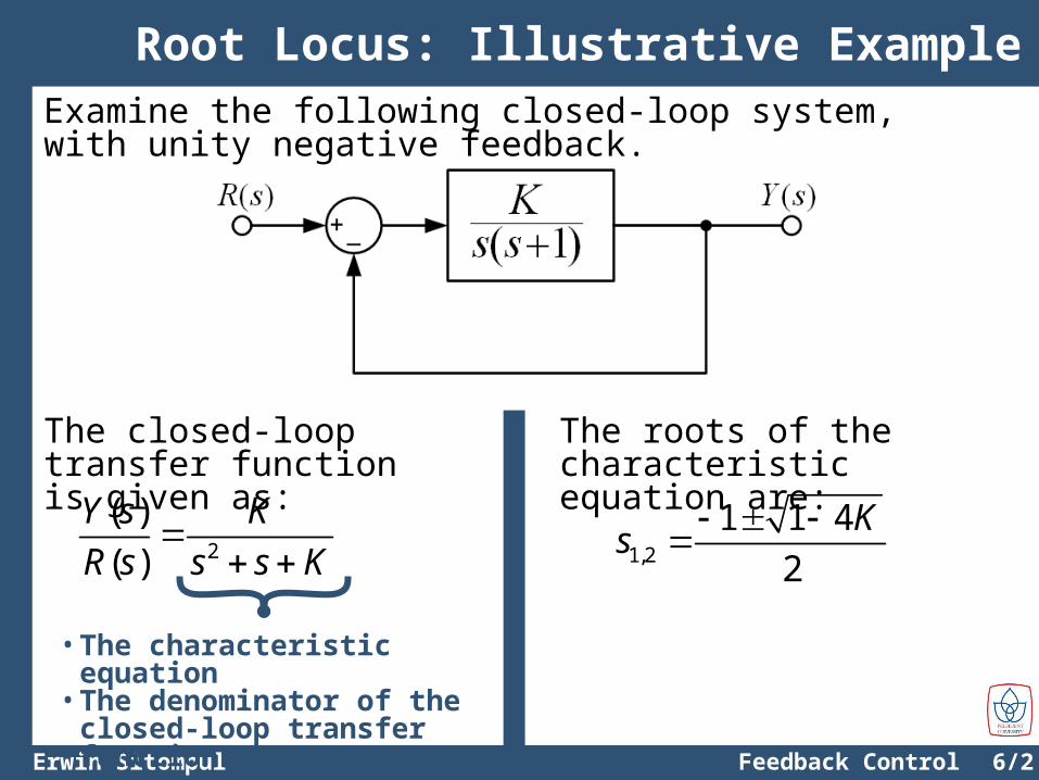
Root Locus: Illustrative ExampleExamine the following closed-loop system, with unity negative feedback.
2
( )
( )
Y s K
R s s s K
1,2
1 1 4
2
Ks
The closed-loop transfer function is given as:
The roots of the characteristic equation are:
• The characteristic equation• The denominator of the
closed-loop transfer function
6/3Erwin Sitompul Feedback Control System
Real Axis
Imag
inar
y A
xis
-2 -1 0 1-2
-1
0
1
2
1,2
1 1 4 1, 0
2 2 4
1 4 1 1,
2 2 4
KK
sK
j K
Root Locus: Illustrative Example
K=0K=0
K=1/4
K=∞
K=∞
: the poles of open-loop transfer function
6/4Erwin Sitompul Feedback Control System
Real Axis
Imag
inar
y A
xis
-2 -1 0 1-1.5
-1
-0.5
0
0.5
1
1.5
Root Locus: Illustrative Example
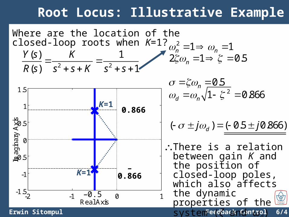
Where are the location of the closed-loop roots when K=1?
2 2
( ) 1
( ) 1
Y s K
R s s s K s s
2 1 0.5n
2 1 1n n
0.5n 21 0.866d n
( ) ( 0.5 0.866)dj j
K=1
K=1
–0.5
–0.866
0.866
There is a relation between gain K and the position of closed-loop poles, which also affects the dynamic properties of the system (ζ and ωd)
6/5Erwin Sitompul Feedback Control System
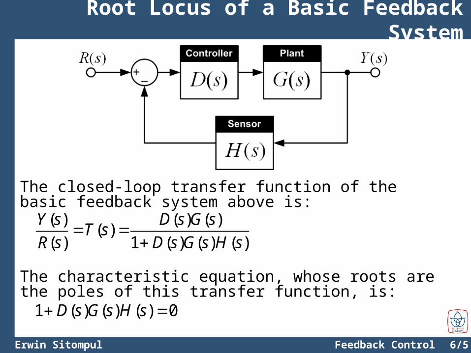
Root Locus of a Basic Feedback System
The closed-loop transfer function of the basic feedback system above is:
( ) ( ) ( )( )
( ) 1 ( ) ( ) ( )
Y s D s G sT s
R s D s G s H s
The characteristic equation, whose roots are the poles of this transfer function, is:
1 ( ) ( ) ( ) 0D s G s H s
6/6Erwin Sitompul Feedback Control System
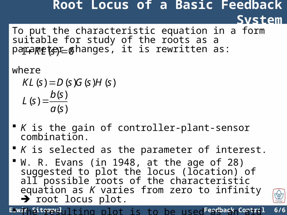
Root Locus of a Basic Feedback SystemTo put the characteristic equation in a form suitable for study of the roots as a parameter changes, it is rewritten as:
1 ( ) 0KL s
where( ) ( ) ( ) ( )KL s D s G s H s
( )( )
( )
b sL s
a s
K is the gain of controller-plant-sensor combination. K is selected as the parameter of interest. W. R. Evans (in 1948, at the age of 28) suggested to plot
the locus (location) of all possible roots of the characteristic equation as K varies from zero to infinity root locus plot.
The resulting plot is to be used as an aid in selecting the best value of K.
6/7Erwin Sitompul Feedback Control System
1 ( ) 0KL s
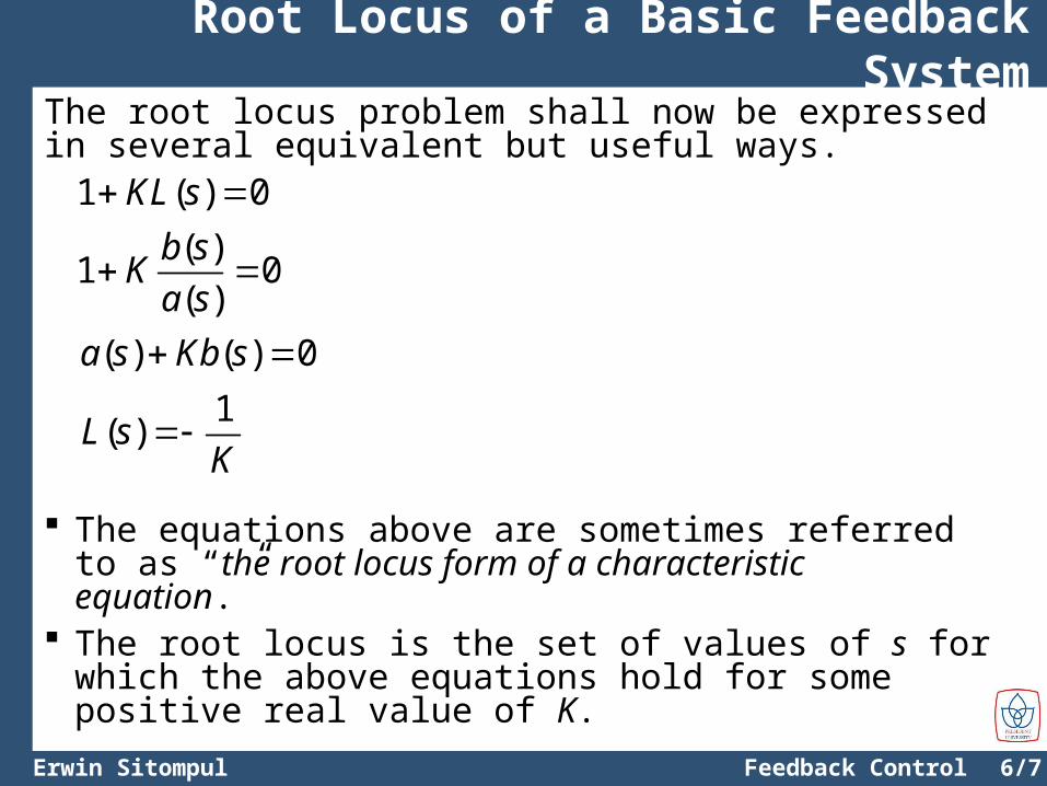
Root Locus of a Basic Feedback SystemThe root locus problem shall now be expressed in several equivalent but useful ways.
( )1 0
( )
b sKa s
( ) ( ) 0a s Kb s 1
( )L sK
The equations above are sometimes referred to as “the root locus form of a characteristic equation.”
The root locus is the set of values of s for which the above equations hold for some positive real value of K.
6/8Erwin Sitompul Feedback Control System
Root Locus of a Basic Feedback System
Explicit solutions are difficult to obtain for higher-order system General rules for the construction of a root locus were developed by Evans.
With the availability of MATLAB, plotting a root locus becomes very easy, using the command “rlocus(num,den)”.
However, in control design we are also interested in how to modify the dynamic response so that a system can meet the specifications for good control performance.
For this purpose, it is very useful to be able to roughly sketch a root locus which will be used to examine a system and to evaluate the consequences of possible compensation alternatives.
Also, it is important to be able to quickly evaluate the correctness of a MATLAB-generated locus to verify that what is plotted is in fact what was meant to be plotted.
6/9Erwin Sitompul Feedback Control System
Guideines for Sketching a Root Locus
1 ( ) 0KL s 1
( )L sK
( ) 1
( )
b s
a s K
Deriving using the root locus form of characteristic equation,
1 2
1 2
( )( ) ( ) 1
( )( ) ( )m
n
s z s z s z
s p s p s p K
Taking the polynomial a(s) and b(s) to be monic, i.e., the coefficient of the highest power of s equals1, they can be factorized as:
If any s = s0 fulfills the equation above, then s0 is said to be on the root locus.
6/10Erwin Sitompul Feedback Control System
0
1 2
1 2
( ) ( ) ( ) 1 1
( ) ( ) ( )m
n s s
s z s z s z
s p s p s p K K
0
1 2
1 2
( )( ) ( ) 1180
( )( ) ( )m
n s s
s z s z s z
s p s p s p K
Phase Condition
Magnitude Condition
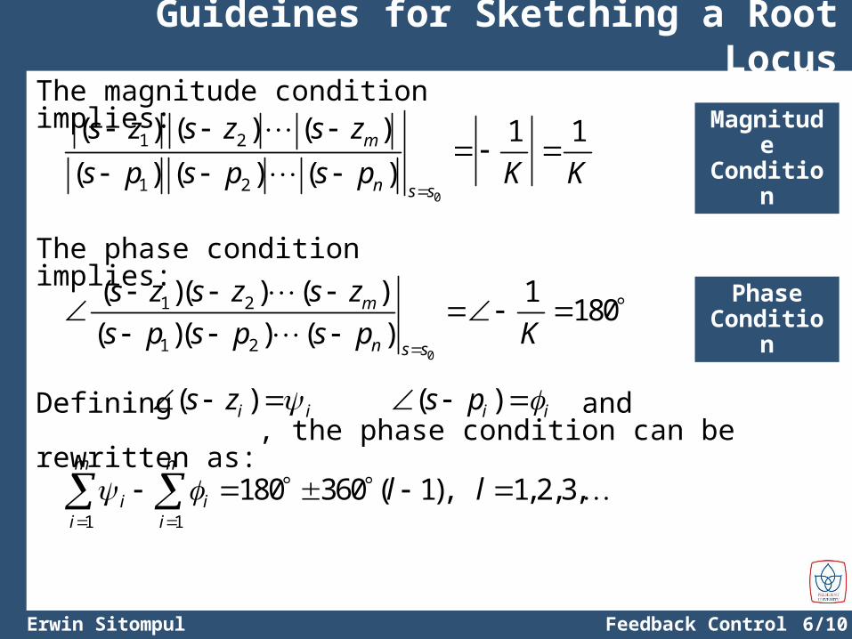
Guideines for Sketching a Root LocusThe magnitude condition implies:
The phase condition implies:
Defining and , the phase condition can be rewritten as:
( )i is z ( )i is p
1 1
180 360 ( 1), 1, 2,3,m n
i ii i
l l
6/11Erwin Sitompul Feedback Control System
Guideines for Sketching a Root Locus
The root locus is the set of values of s for which 1 + KL(s) = 0 is satisfied as the real parameter K varies from 0 to ∞. Typically, 1 + KL(s) = 0 is the characteristic equation of the system, and in this case the roots on the locus are the closed-loop poles of that system.
“
”The root locus of L(s) is the set of points in the s-plane where the phase of L(s) is 180°. If the angle to a test point from a zero is defined as ψi and the angle to a test point from a pole as Φi, then the root locus of L(s) is expressed as those points in the s-plane where, for integer l, Σψi – ΣΦi = 180° + 360°(l–1).
“
”
6/12Erwin Sitompul Feedback Control System
Guideines for Sketching a Root Locus
2
1( )
( 5) ( 2) 4
sL s
s s s
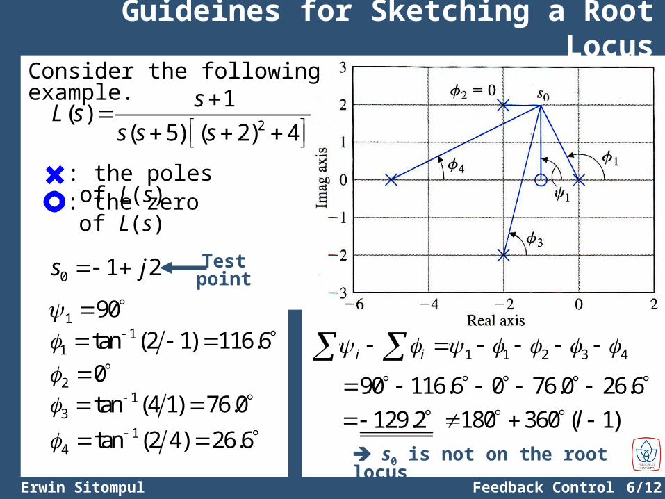
Consider the following example.
: the poles of L(s): the zero of L(s)
0 1 2s j Test point
1 90 1
1 tan (2 1) 116.6
2 0 1
3 tan (4 1) 76.0 1
4 tan (2 4) 26.6
1 1 2 3 4i i 90 116.6 0 76.0 26.6
129.2 180 360 ( 1)l s0 is not on the root locus
6/13Erwin Sitompul Feedback Control System
Rules for Plotting a Root Locus
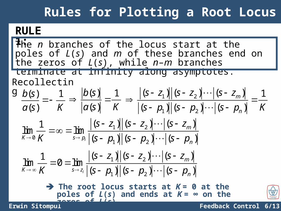
RULE 1:The n branches of the locus start at the poles of L(s) and m of these branches end on the zeros of L(s), while n–m branches terminate at infinity along asymptotes.
( ) 1
( )
b s
a s K
Recollecting( ) 1
( )
b s
a s K
1 2
01 2
( ) ( ) ( )1lim lim
( ) ( ) ( )i
m
K s pn
s z s z s z
K s p s p s p
1 2
1 2
( ) ( ) ( ) 1
( ) ( ) ( )m
n
s z s z s z
s p s p s p K
1 2
1 2
( ) ( ) ( )1lim 0 lim
( ) ( ) ( )i
m
K s zn
s z s z s z
K s p s p s p
The root locus starts at K = 0 at the poles of L(s) and ends at K = ∞ on the zeros of L(s)
6/14Erwin Sitompul Feedback Control System
Rules for Plotting a Root Locus
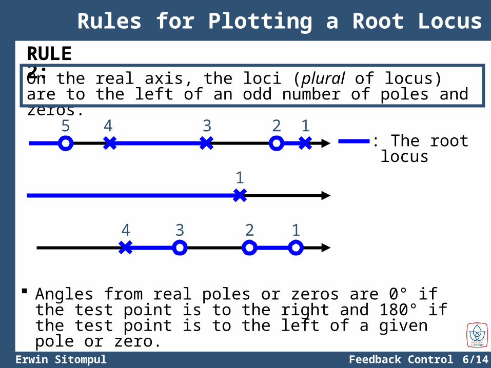
RULE 2:On the real axis, the loci (plural of locus) are to the left of an odd number of poles and zeros.
12345: The root locus
1
1234
Angles from real poles or zeros are 0° if the test point is to the right and 180° if the test point is to the left of a given pole or zero.
6/15Erwin Sitompul Feedback Control System
2
1( )
( 4) 16L s
s s
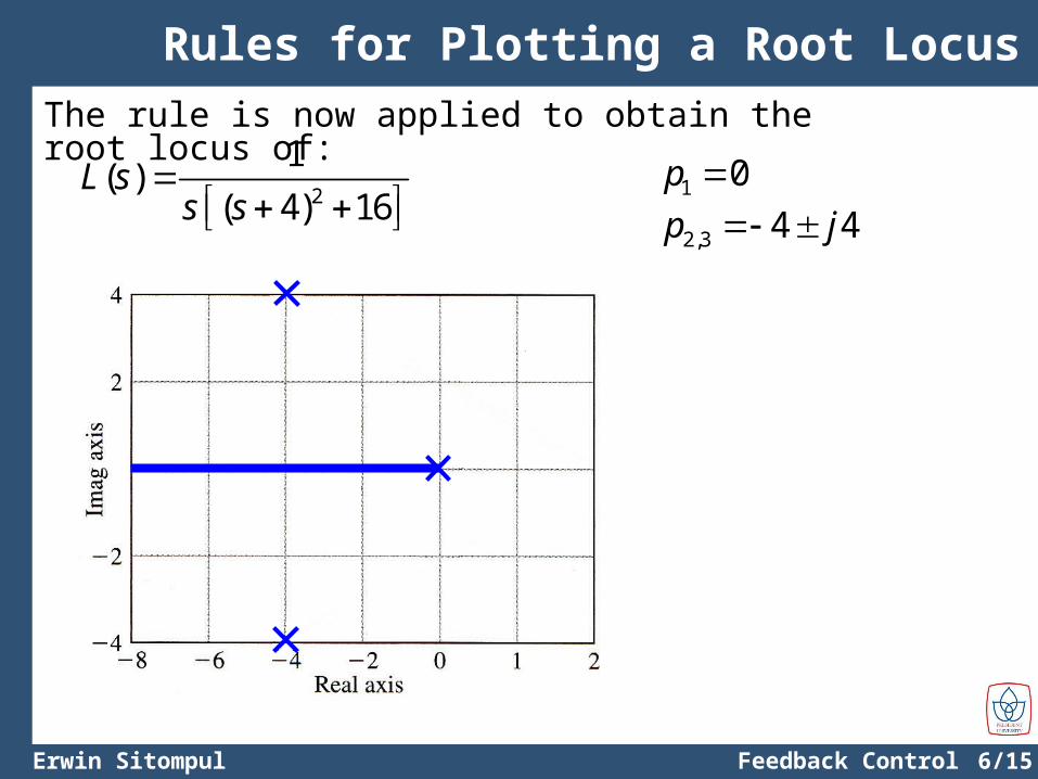
Rules for Plotting a Root Locus
The rule is now applied to obtain the root locus of:
2,3 4 4p j 1 0p
6/16Erwin Sitompul Feedback Control System
Rules for Plotting a Root Locus
1 2 3 0
180 360 ( 1)l
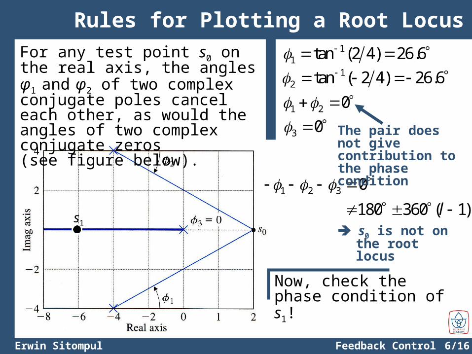
For any test point s0 on the real axis, the angles φ1 and φ2 of two complex conjugate poles cancel each other, as would the angles of two complex conjugate zeros (see figure below).
11 tan (2 4) 26.6
12 tan ( 2 4) 26.6
1 2 0
3 0 The pair does not give contribution to the phase condition
s0 is not on the root locus
Now, check the phase condition of s1!
s1
6/17Erwin Sitompul Feedback Control System
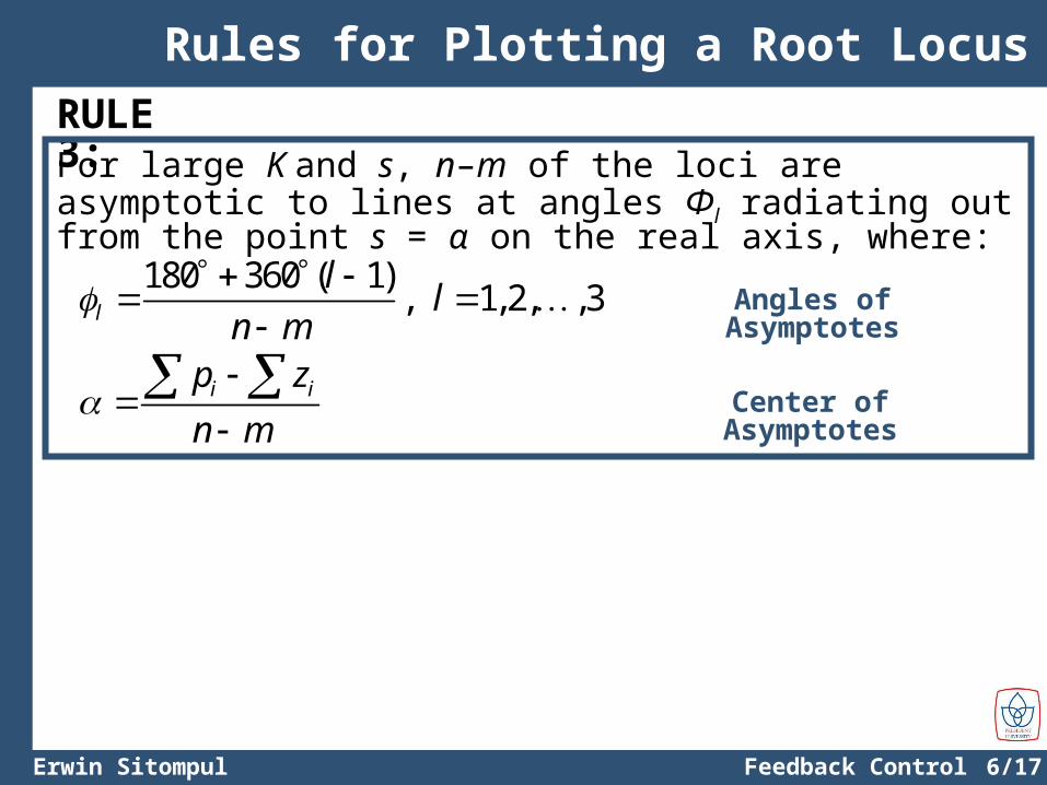
RULE 3:For large K and s, n–m of the loci are asymptotic to lines at angles Φl radiating out from the point s = α on the real axis, where:
Rules for Plotting a Root Locus
180 360 ( 1), 1, 2, ,3l
ll
n m
i ip z
n m
Center of Asymptotes
Angles of Asymptotes
6/18Erwin Sitompul Feedback Control System
Rules for Plotting a Root Locus
2
1( )
( 4) 16L s
s s
For , we obtain
1 2,30, 4 4p p j 3, 0n m
180 360 ( 1)
3 0
l
i ip z
n m
60 120 ( 1)l 60 ,180 ,300
180 360 ( 1)l
l
n m
( 4 4) ( 4 4) 0
3 0
j j
8
2.673
–2.67
60°
180°
300°
6/19Erwin Sitompul Feedback Control System
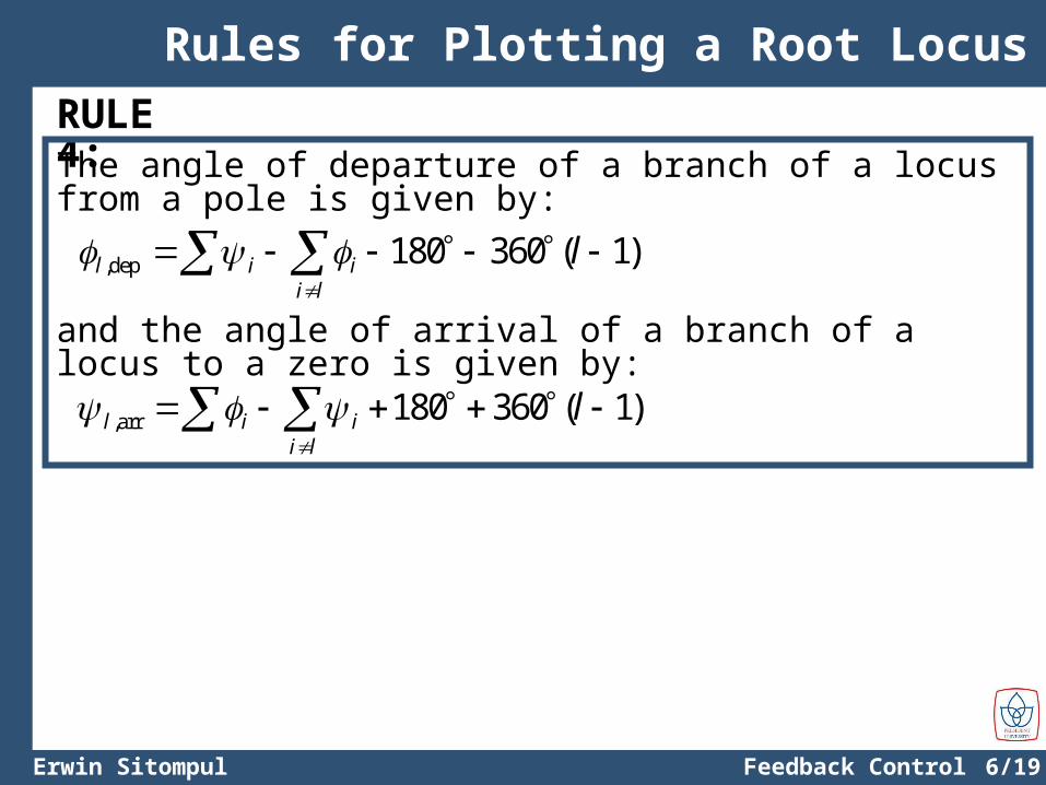
RULE 4:The angle of departure of a branch of a locus from a pole is given by:
Rules for Plotting a Root Locus
,dep 180 360 ( 1)l i ii l
l
and the angle of arrival of a branch of a locus to a zero is given by:
,arr 180 360 ( 1)l i ii l
l
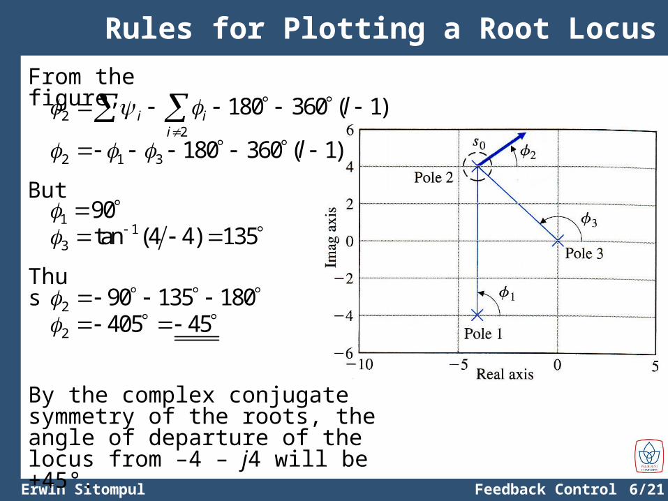
6/20Erwin Sitompul Feedback Control System
Rules for Plotting a Root Locus
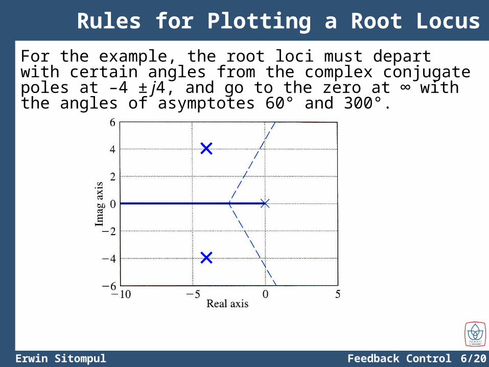
For the example, the root loci must depart with certain angles from the complex conjugate poles at –4 ± j4, and go to the zero at ∞ with the angles of asymptotes 60° and 300°.
6/21Erwin Sitompul Feedback Control System
Rules for Plotting a Root Locus
22
180 360 ( 1)i ii
l
2 1 3 180 360 ( 1)l
13 tan (4 4) 135 1 90
2 90 135 180 2 405 45
From the figure,
But
Thus
By the complex conjugate symmetry of the roots, the angle of departure of the locus from –4 – j4 will be +45°.
6/22Erwin Sitompul Feedback Control System
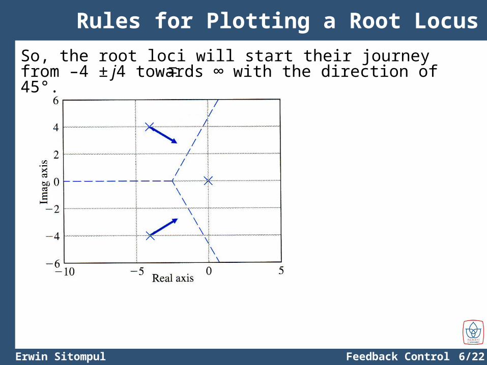
Rules for Plotting a Root Locus
So, the root loci will start their journey from –4 ± j4 towards ∞ with the direction of 45°.
±
6/23Erwin Sitompul Feedback Control System
Rules for Plotting a Root Locus
RULE 5:The locus crosses the jω axis (imaginary axis) at points where: The Routh criterion shows a transition from roots in the left
half-plane to roots in the right half-plane. This transition means that the closed-loop system is
becoming unstable. This fact can be tested by Routh’s stability criterion, with
K as the parameter, where an incremental change of K will cause the sign change of an element in the first column of Routh’s array.
The values of s = ± jω0 are the solution of the characteristic equation in root locus form, 1 + KL(s) = 0. The points ± jω0 are the points of cross-over on the
imaginary axis.
6/24Erwin Sitompul Feedback Control System
Rules for Plotting a Root Locus
For the example, the characteristic equation can be written as:
1 ( ) 0KL s
2
11 0
( 4) 16Ks s
3 28 32 0s s s K
3
2
1
0
: 1 32
: 8
8 32:
8:
s
s K
Ks
s K
The closed-loop system is stable for K > 0 and K < 256 for 0 < K < 256.
For K > 256 there are 2 roots in the RHP (two sign changes in the first column).
For K = 256 the roots must be on the imaginary axis.

6/25Erwin Sitompul Feedback Control System
3 28 32 256 0s s s
The characteristic equation is now solved using K = 256.
1
2,3 0
85.66
ss j j Points of Cross-over
Another way to solve for ω0 is by simply replacing any s with jω0 without finding the value of K first.
3 20 0 0( ) 8( ) 32( ) 0j j j K
3 20 0 08 32 0j j K
2 30 0 08 (32 ) 0K j
≡ 0 ≡ 0
30 0
20
0
32 32 5.66
208
8 32 256
KKK
Rules for Plotting a Root Locus
Same results for K and ω0
6/26Erwin Sitompul Feedback Control System
5.66
–5.66
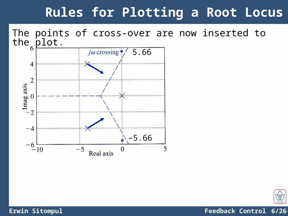
Rules for Plotting a Root Locus
The points of cross-over are now inserted to the plot.
6/27Erwin Sitompul Feedback Control System
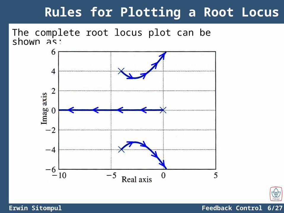
Rules for Plotting a Root Locus
The complete root locus plot can be shown as:
6/28Erwin Sitompul Feedback Control System
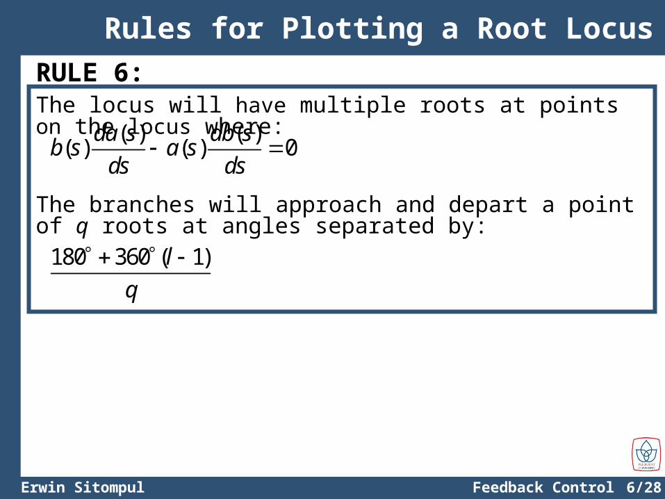
Rules for Plotting a Root Locus
RULE 6:The locus will have multiple roots at points on the locus where:
( ) ( )( ) ( ) 0da s db s
b s a sds ds
The branches will approach and depart a point of q roots at angles separated by:
180 360 ( 1)l
q
6/29Erwin Sitompul Feedback Control System
Rules for Plotting a Root Locus
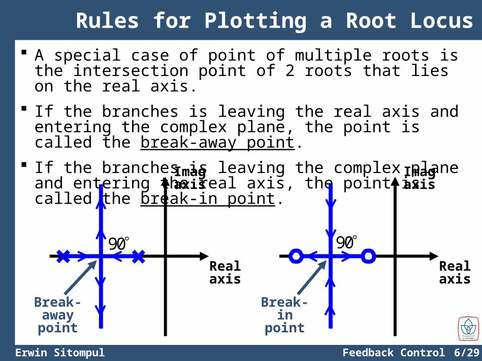
A special case of point of multiple roots is the intersection point of 2 roots that lies on the real axis.
If the branches is leaving the real axis and entering the complex plane, the point is called the break-away point.
If the branches is leaving the complex plane and entering the real axis, the point is called the break-in point.
Realaxis
Imagaxis
Break-awaypoint
Realaxis
Imagaxis
Break-inpoint
90 90
6/30Erwin Sitompul Feedback Control System
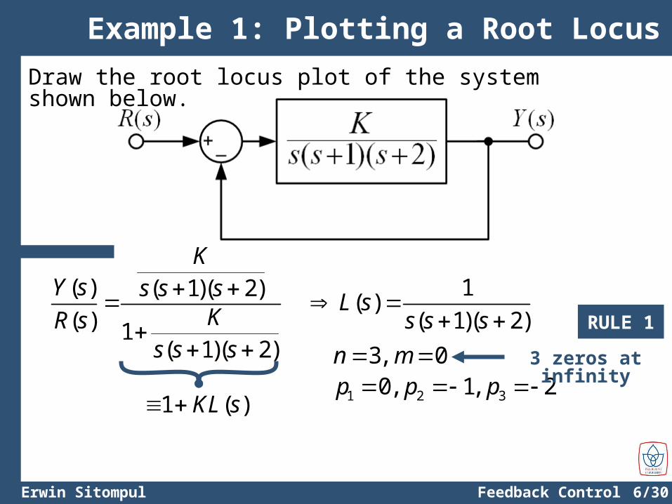
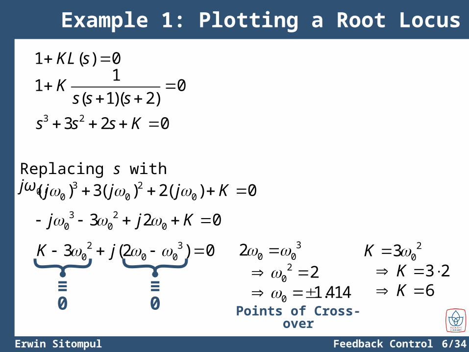
Example 1: Plotting a Root Locus
Draw the root locus plot of the system shown below.
1( )
( 1)( 2)L s
s s s
1 2 30, 1, 2p p p 3, 0n m 3 zeros at infinity
RULE 1
( ) ( 1)( 2)( ) 1
( 1)( 2)
KY s s s s
KR ss s s
1 ( )KL s
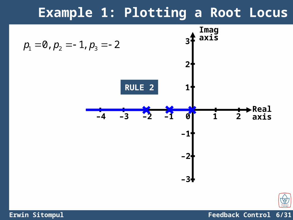
6/31Erwin Sitompul Feedback Control System
Example 1: Plotting a Root Locus
Realaxis
Imagaxis
1 20–1–2–3–4
1
2
–1
–2
3
–3
RULE 2
1 2 30, 1, 2p p p
6/32Erwin Sitompul Feedback Control System
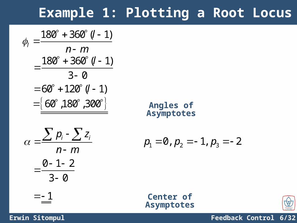
Example 1: Plotting a Root Locus
180 360 ( 1)l
l
n m
180 360 ( 1)
3 0
l
i ip z
n m
60 120 ( 1)l 60 ,180 ,300
0 1 2
3 0
1
1 2 30, 1, 2p p p
Center of Asymptotes
Angles of Asymptotes
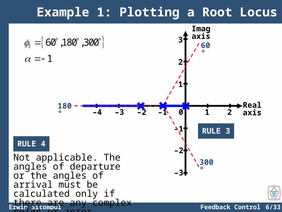
6/33Erwin Sitompul Feedback Control System
Example 1: Plotting a Root Locus
Realaxis
Imagaxis
1 20–1–2–3–4
1
2
–1
–2
3
–3
RULE 3
60°
180°
300°
60 ,180 ,300l
1
Not applicable. The angles of departure or the angles of arrival must be calculated only if there are any complex poles or zeros.
RULE 4
6/34Erwin Sitompul Feedback Control System
Example 1: Plotting a Root Locus
1 ( ) 0KL s 1
1 0( 1)( 2)
Ks s s
3 23 2 0s s s K
Replacing s with jω0,3 2
0 0 0( ) 3( ) 2( ) 0j j j K 3 2
0 0 03 2 0j j K 2 3
0 0 03 (2 ) 0K j
≡ 0 ≡ 0
30 0
20
0
2 2 1.414
203
3 2 6
KKK
Points of Cross-over
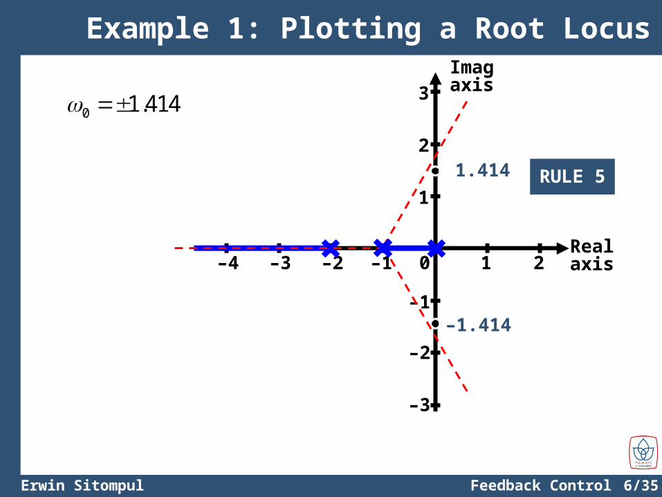
6/35Erwin Sitompul Feedback Control System
Example 1: Plotting a Root Locus
Realaxis
Imagaxis
1 20–1–2–3–4
1
2
–1
–2
3
–3
RULE 51.414
–1.414
0 1.414
6/36Erwin Sitompul Feedback Control System
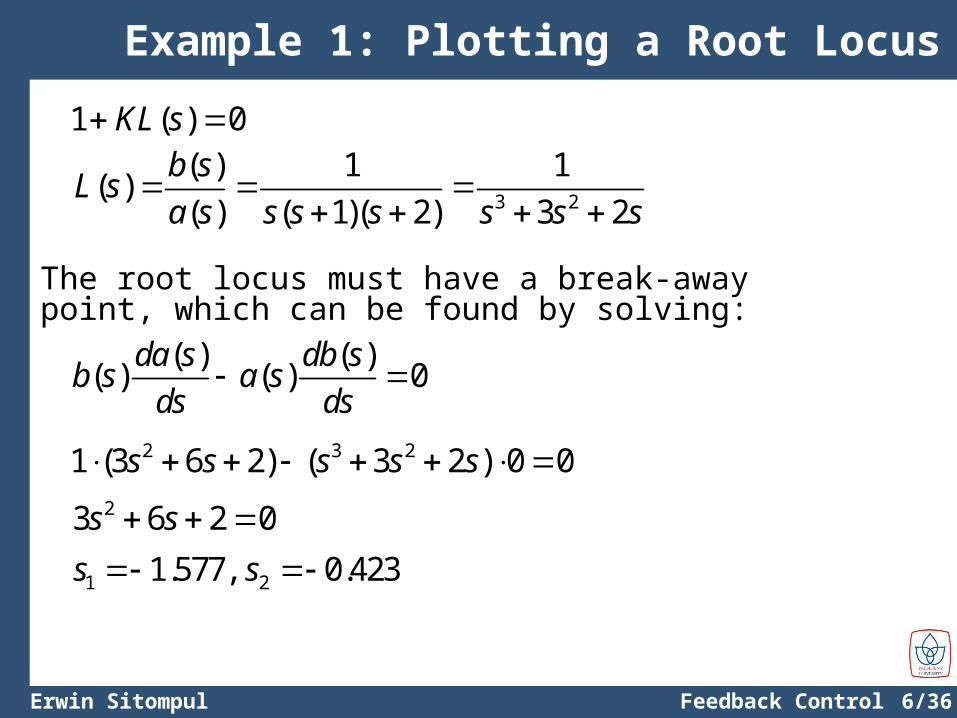
Example 1: Plotting a Root Locus
1 ( ) 0KL s
3 2
( ) 1 1( )
( ) ( 1)( 2) 3 2
b sL s
a s s s s s s s
( ) ( )( ) ( ) 0da s db s
b s a sds ds
The root locus must have a break-away point, which can be found by solving:
2 3 21 (3 6 2) ( 3 2 ) 0 0s s s s s 23 6 2 0s s
1 21.577, 0.423s s
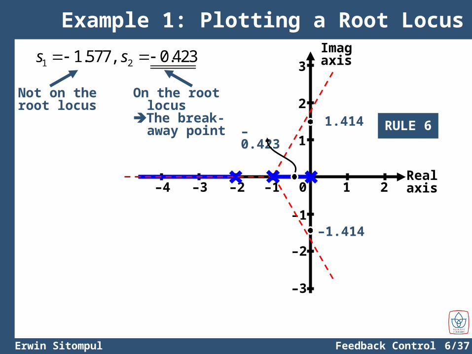
6/37Erwin Sitompul Feedback Control System
Example 1: Plotting a Root Locus
Realaxis
Imagaxis
1 20–1–2–3–4
1
2
–1
–2
3
–3
RULE 61.414
–1.414
1 21.577, 0.423s s
On the root locusThe break-away
point
Not on the root locus
–0.423
6/38Erwin Sitompul Feedback Control System
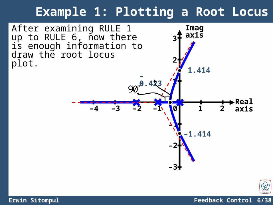
Example 1: Plotting a Root LocusAfter examining RULE 1 up to RULE 6, now there is enough information to draw the root locus plot.
Realaxis
Imagaxis
1 20–1–2–3–4
1
2
–1
–2
3
–3
1.414
–1.414
–0.423
90
6/39Erwin Sitompul Feedback Control System
Example 1: Plotting a Root Locus
Realaxis
Imagaxis
1 20–1–2–3–4
1
2
–1
–2
3
–3
1.414
–1.414
–0.423
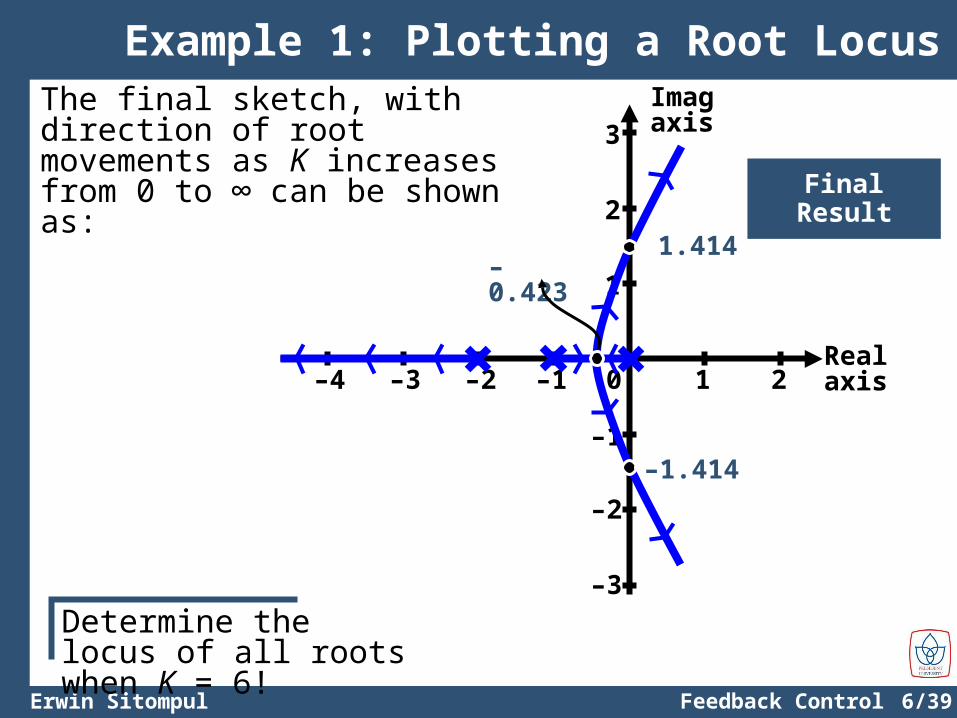
The final sketch, with direction of root movements as K increases from 0 to ∞ can be shown as:
Final Result
Determine the locus of all roots when K = 6!
6/40Erwin Sitompul Feedback Control System
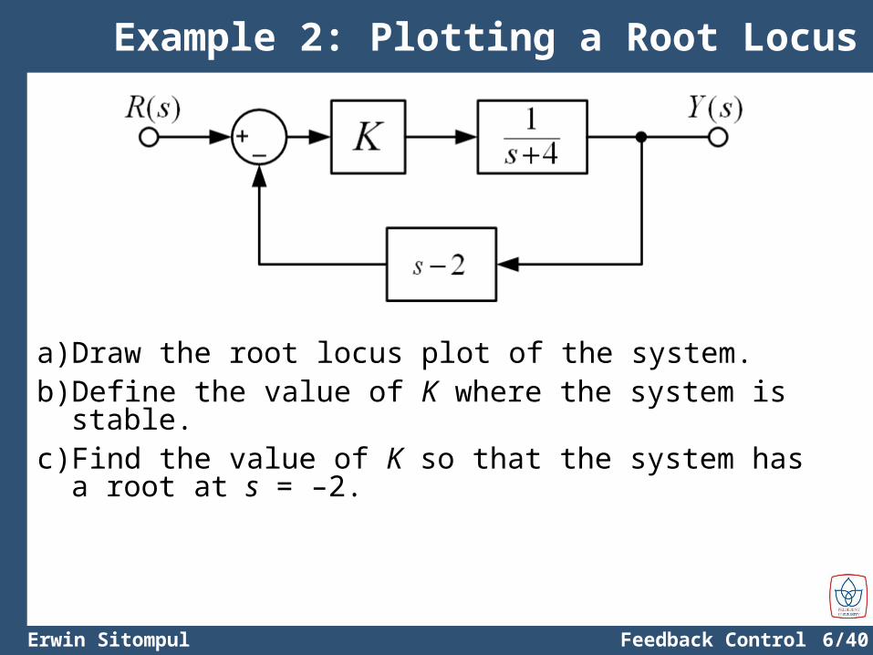
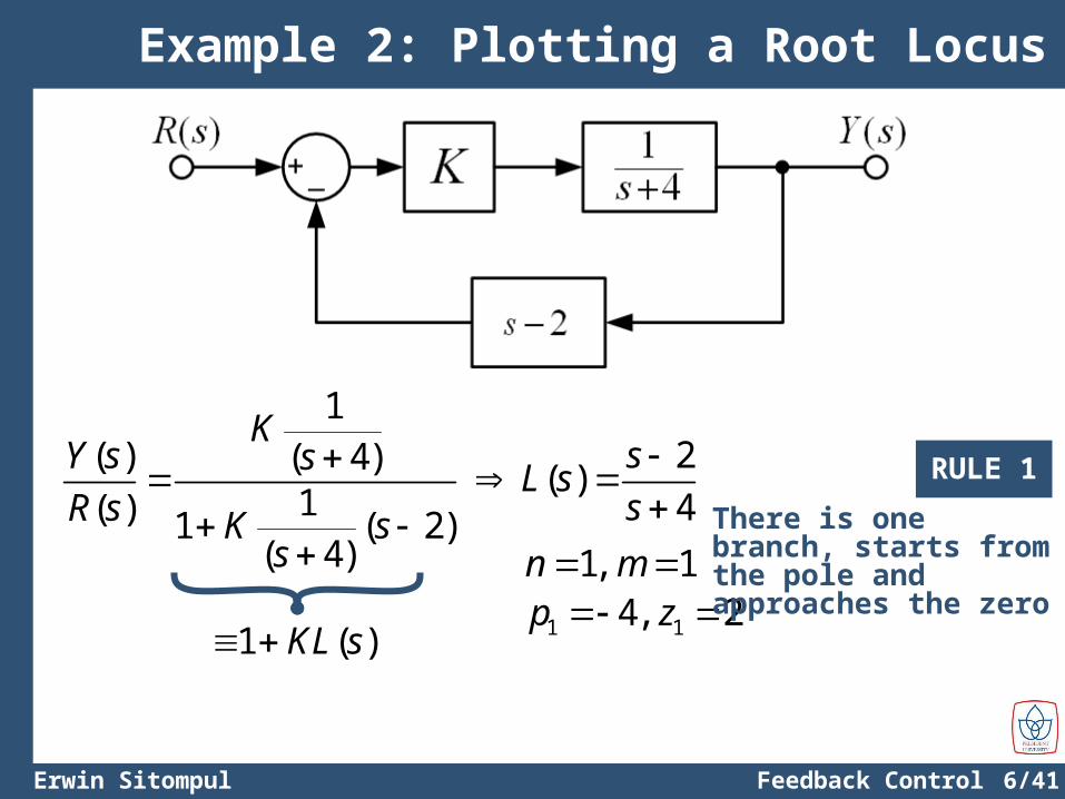
Example 2: Plotting a Root Locus
a) Draw the root locus plot of the system.b) Define the value of K where the system is stable.c) Find the value of K so that the system has a root at s = –2.
6/41Erwin Sitompul Feedback Control System
Example 2: Plotting a Root Locus
1( ) ( 4)
1( ) 1 ( 2)( 4)
KY s sR s K s
s
2( )
4
sL s
s
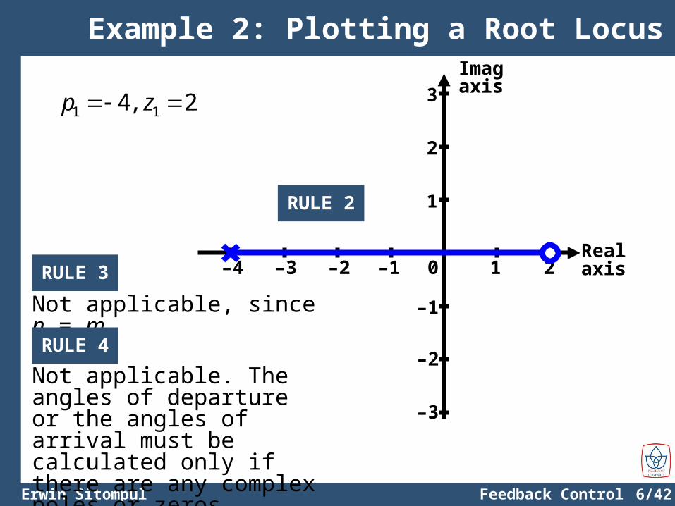
1 14, 2p z 1, 1n m
1 ( )KL s
RULE 1
There is one branch, starts from the pole and approaches the zero
6/42Erwin Sitompul Feedback Control System
Example 2: Plotting a Root Locus
Realaxis
Imagaxis
1 20–1–2–3–4
1
2
–1
–2
3
–3
RULE 2
1 14, 2p z
Not applicable, since n = m.
RULE 3
Not applicable. The angles of departure or the angles of arrival must be calculated only if there are any complex poles or zeros.
RULE 4
6/43Erwin Sitompul Feedback Control System
Example 2: Plotting a Root Locus
1 ( ) 0KL s 2
1 04
sKs
4 ( 2) 0s K s
Replacing s with jω0,
0 0( ) 4 ( 2) 0j K j
04 2 (1 ) 0K j K
≡ 0 ≡ 0
4 2 2
KK
0
0
(1 ) 0
K
Points of Cross-over
6/44Erwin Sitompul Feedback Control System
Example 2: Plotting a Root Locus
Realaxis
Imagaxis
1 20–1–2–3–4
1
2
–1
–2
3
–3
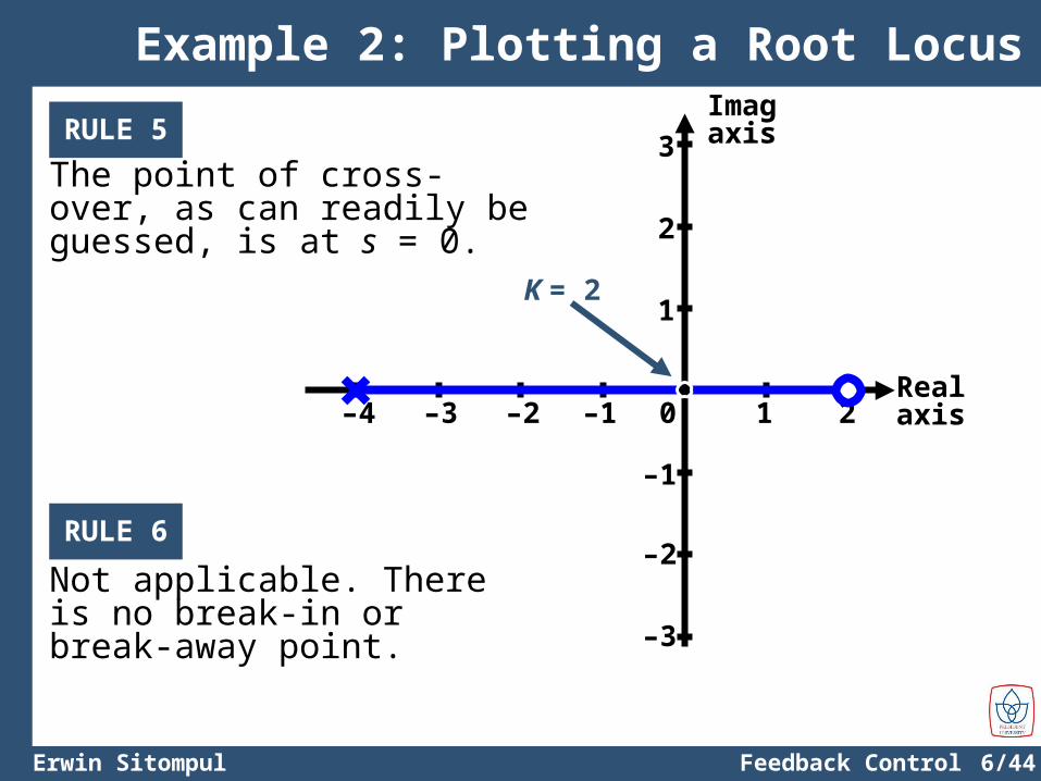
The point of cross-over, as can readily be guessed, is at s = 0.
RULE 5
Not applicable. There is no break-in or break-away point.
RULE 6
K = 2
6/45Erwin Sitompul Feedback Control System
Example 2: Plotting a Root Locus
Realaxis
Imagaxis
1 20–1–2–3–4
1
2
–1
–2
3
–3
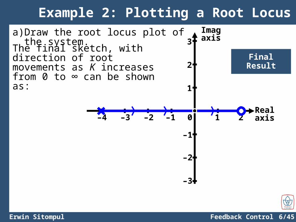
The final sketch, with direction of root movements as K increases from 0 to ∞ can be shown as:
Final Result
a) Draw the root locus plot of the system.
6/46Erwin Sitompul Feedback Control System
Example 2: Plotting a Root Locus
Realaxis
Imagaxis
1 20–1–2–3–4
1
2
–1
–2
3
–3
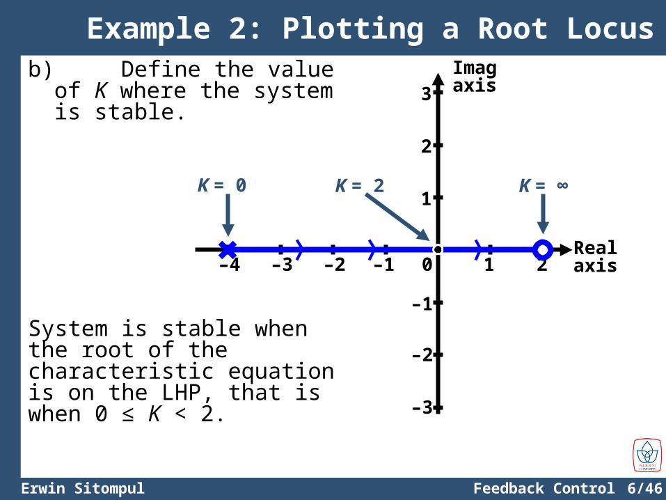
b) Define the value of K where the system is stable.
System is stable when the root of the characteristic equation is on the LHP, that is when 0 ≤ K < 2.
K = 2K = 0 K = ∞
6/47Erwin Sitompul Feedback Control System
Example 2: Plotting a Root Locus
Realaxis
Imagaxis
1 20–1–2–3–4
1
2
–1
–2
3
–3
K = 2K = 0 K = ∞
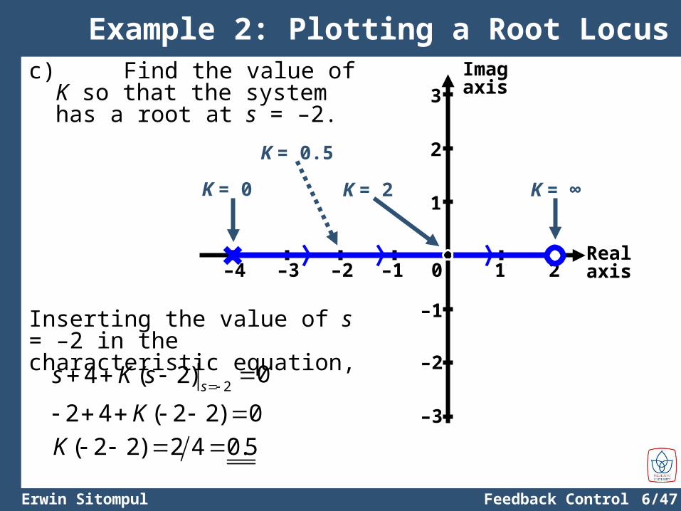
c) Find the value of K so that the system has a root at s = –2.
Inserting the value of s = –2 in the characteristic equation,
204 ( 2)
ss K s
2 4 ( 2 2) 0K ( 2 2) 2 4 0.5K
K = 0.5
6/48Erwin Sitompul Feedback Control System
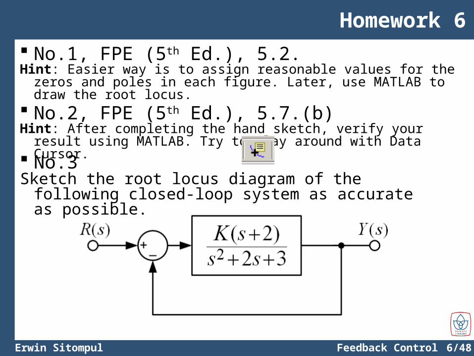
Homework 6 No.1, FPE (5th Ed.), 5.2.Hint: Easier way is to assign reasonable values for the zeros and poles in
each figure. Later, use MATLAB to draw the root locus.
No.3Sketch the root locus diagram of the following closed-loop
system as accurate as possible.
No.2, FPE (5th Ed.), 5.7.(b)Hint: After completing the hand sketch, verify your result using MATLAB. Try
to play around with Data Cursor.
Related Documents


