Feedback control of solid oxide fuel cell spatial temperature variation

Page 1

F

MD

a

ARR1AA

KSSHDDL

1

arrbgaettblt

bmpasS

0d

Journal of Power Sources 195 (2010) 4222–4233

Contents lists available at ScienceDirect

Journal of Power Sources

journa l homepage: www.e lsev ier .com/ locate / jpowsour

eedback control of solid oxide fuel cell spatial temperature variation

ahshid Fardadi, Fabian Mueller ∗, Faryar Jabbariepartment of Mechanical and Aerospace Engineering, University of California, Irvine, CA 92697, United States

r t i c l e i n f o

rticle history:eceived 13 November 2009eceived in revised form9 December 2009ccepted 22 December 2009vailable online 13 January 2010

eywords:olid oxide fuel cell

a b s t r a c t

A high performance feedback controller has been developed to minimize SOFC spatial temperature vari-ation following significant load perturbations. For thermal management, spatial temperature variationalong SOFC cannot be avoided. However, results indicate that feedback control can be used to manipulatethe fuel cell air flow and inlet fuel cell air temperature to maintain a nearly constant SOFC electrode elec-trolyte assembly temperature profile. For example temperature variations of less than 5 K are obtainedfor load perturbations of ±25% from nominal. These results are obtained using a centralized controlstrategy to regulate a distributed temperature profile and manage actuator interactions. The controller isbased on H-infinity synthesis using a physical based dynamic model of a single co-flow SOFC repeat cell.

patial temperature control-infinityynamic modelingisturbance rejectionoad following

The model of the fuel cell spatial temperature response needed for control synthesis was linearized andreduced from nonlinear model of the fuel cell assembly. A single 11 state feedback linear system testedin the full nonlinear model was found to be effective and stable over a wide fuel cell operating envelope(0.82–0.6 V). Overall, simulation of the advanced controller resulted in small and smooth monotonic tem-perature response to rapid and large load perturbations. This indicates that future SOFC systems can bedesigned and controlled to have superb load following characteristic with less than previously expected

thermal stresses.

. Introduction and background

There is much interest in the shift from fossil fuel to renew-ble based energy infrastructures to secure energy supplies andeduce environmental impacts (for example see [1–3]). To maintaineliable and dependable energy generation, with increased contri-utions from renewable sources, a much larger role for dispatchableeneration will be required. High temperature fuel cell systems aren attractive solution with ultra low pollutant emissions and highfficiency—particularly if used in hybrid arrangements. The abilityo achieve high efficiencies on smaller scales opens the door for dis-ributed generation and use of renewable biogas. To fully exploit theenefits of this new paradigm, the fuel cell must have a relatively

arge envelop of transient operation (changes in power demand orhe supply of renewable fuel).

High temperature fuel cells are currently being deployed asase-loaded system as the technology is slowly overcoming theany engineering challenges to be competitive in the market

lace. In particular, transient operation of SOFC system can be veryttractive. Simulations indicate that well designed integrated SOFCystems can load follow very rapidly [4–9]. The current drawn fromOFC can be increased at the rate of electrochemistry, on the order

∗ Corresponding author. Tel.: +1 949 824 6602; fax: +1 949 824 7423.E-mail address: [email protected] (F. Mueller).

378-7753/$ – see front matter © 2010 Elsevier B.V. All rights reserved.oi:10.1016/j.jpowsour.2009.12.111

© 2010 Elsevier B.V. All rights reserved.

of milliseconds, with increased efficiency at part load, and ultra lowpollutant emissions for the whole range of operation (see [10] fora list of SOFC attributes).

A major issue inhibiting transient SOFC operation is that thermalstresses during transient operation can increase the probability offailure and degradation of the fuel cell (e.g., see [11–14]). To mini-mize thermal stresses and the corresponding probability of failure,it is critical to minimize spatial temperature variations during SOFCoperation. The goal of this paper is to evaluate the ability to mini-mize fuel cell spatial temperature variations, during transients.

Transient operation of solid oxide fuel cell requires advancedintegrated system controls as explored in [4,7,9,15,16] to maintainthe system within operating requirements. Exact SOFC system con-troller design can vary depending on the SOFC system design andconfiguration. However, all fuel cell systems will generally requirea (1) system power controller, (2) a fuel utilization/combustortemperature controller, and (3) a fuel cell stack temperature con-troller. The first two have received ample attention, for examplesee [4,5,7,16,17]. The focus of this paper is on spatial temperaturecontrol. Since fuel cell temperature response time constants areconsiderably larger than fuel and electrochemical response and dif-

ferent actuators are used for fuel, electrochemical and temperaturecontrol, it is possible to decouple fuel cell temperature control fromthe more rapid fuel flow and fuel cell current control.

Fuel cells are thermally managed by control of air through thefuel cell. Temperature increase in the air flow direction of the fuel

Page 2

M. Fardadi et al. / Journal of Power So

Nomenclature

C solid specific heat capacity [kJ kg−1 K−1]CV constant volume gas specific heat capacityE voltage polarization [V]F Faradays constant [96,487 C mol−1]h enthalpy [kJ kmol−1]hf enthalpy of formation [kJ kmol−1]i current [A]N molar capacity [kmol]N molar flow rate [kmol s−1]Nu Nusselt number [–]P pressure [kpa], power [kW]� density of solid [kg m-2]Q heat transfer [kW]R species reaction rate [kmol s−1], universal gas con-

stant [8.3145 J mol−1 K−1]t time [s]T temperature [K]V volume [m3], voltage [V]

cspsiceiw

msionfivpo

crcmptitmmstttd

hgbad

2.1. Model discretization

In total the fuel cell is discretized into 20 control volumes (4layers per node times 5 nodes in flow direction), where the top and

W rate of work [kW]X species mole fraction [–]

ell is generally unavoidable and is a critical fuel cell design con-ideration. The nominal full-power operating SOFC temperaturerofile is a trade-off between the fuel cell material durability andystem efficiency. SOFC are made of thin ceramic tri-layer consist-ng of a positive electrode, electrolyte, negative electrode (PEN) thatan crack due to thermal stresses. However, to maximize systemfficiency the fuel cell air flow rate should be minimized resultingn increased temperature gradient and increased thermal stresses

ithin the PEN.Different stack configurations and fuel cell thermal manage-

ent strategies exist in the literature (for examples see [18–20]). Aingle planar fuel cell is considered here, with a 100 K temperaturencrease in the PEN from 1023 to 1123 K, in balanced or nominalperation. The optimization of the nominal temperature profile isot the focus of the paper, since the nominal temperature pro-le is application dependent. The control goal here is to minimizeariation in the fuel cell PEN spatial temperature in time. This isarticularly challenging during load perturbations as the amountf heat generated within the fuel cell changes non-uniformly.

Research has shown that the average temperature of fuel cellsan be effectively managed by manipulating the cathode air flowate through the fuel cell [4–6,21,22]. However, to minimize fuelell degradation, variations in the fuel cell temperature must beinimized. For example, Nakajo et al. [13,23] have shown that

robabilities of failure can increase significantly due to tempera-ure variation during transient. Inui et al. [24] have showed thatt is possible to minimize the spatial temperature variations ofhe fuel cell over a large fuel cell operating envelope by optimally

anipulating both the fuel cell air flow and air inlet temperature toinimize temperature variations. That work is based primarily on

teady-state analysis and is not directly related to transient opera-ion under changing loads or disturbances. This research builds onhe work of Inui et al., to demonstrate the performance of controlso maintain a nominal fuel cell spatial temperature profile, in time,uring load perturbations.

A model with modest levels of spatial distribution is utilized

erein. Due to the uneven distribution of current and thus heateneration, as well as heat conduction and convection, there cane significant variations in the temperature profile of the fuel cell,long the length of the cell. These large variations can lead toamage or failure and average temperature from a bulk model

urces 195 (2010) 4222–4233 4223

would not show the extent of the thermal stress. We start by a fuelcell operating at the baseline condition, based on some maximumoverall efficiency consideration. We then show the temperaturevariations from the temperature profile associated with the base-line condition due to disturbances associated with power demandfluctuations. After linearizing the model about the operating con-ditions, we show the large range of variations that can be capturedby the approximate model. Next, we develop high performancecontrollers that reduce the variations significantly and comparethe results with what could have been obtained from extensivesimulation and off-line optimization (e.g., look-up tables).

Consistent with the work of Inui et al., the air flow rate andinlet temperature are considered as manipulated variables. In SOFCsystem, the air flow rate can be varied either by variable speed com-pressor and blowers (as was explored in [4,5,7,25]) or by air inletguide vanes (see [25]). The air inlet temperature can be manipu-lated by bypassing air recuperators. The air flow rate and air inlettemperature can be manipulated independently to minimize spa-tial temperature variations in time. The results show the potentialfor use of advance control techniques for high performance opera-tion of fuel cell power systems.

2. Dynamic modeling

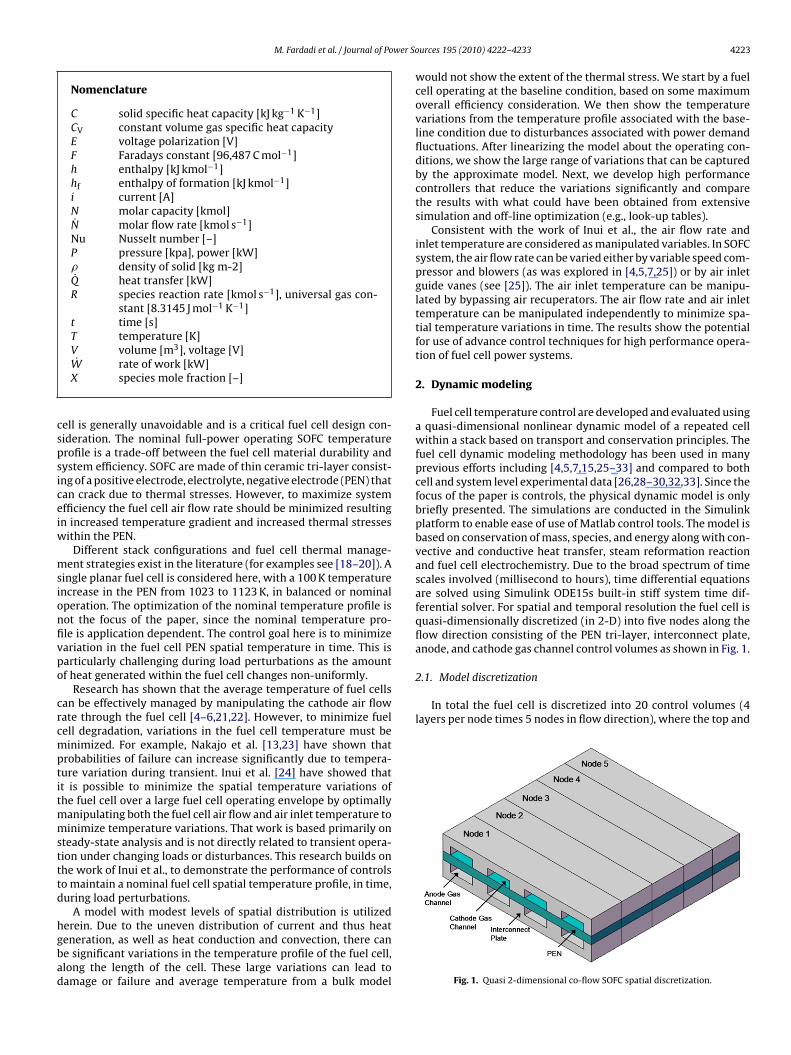
Fuel cell temperature control are developed and evaluated usinga quasi-dimensional nonlinear dynamic model of a repeated cellwithin a stack based on transport and conservation principles. Thefuel cell dynamic modeling methodology has been used in manyprevious efforts including [4,5,7,15,25–33] and compared to bothcell and system level experimental data [26,28–30,32,33]. Since thefocus of the paper is controls, the physical dynamic model is onlybriefly presented. The simulations are conducted in the Simulinkplatform to enable ease of use of Matlab control tools. The model isbased on conservation of mass, species, and energy along with con-vective and conductive heat transfer, steam reformation reactionand fuel cell electrochemistry. Due to the broad spectrum of timescales involved (millisecond to hours), time differential equationsare solved using Simulink ODE15s built-in stiff system time dif-ferential solver. For spatial and temporal resolution the fuel cell isquasi-dimensionally discretized (in 2-D) into five nodes along theflow direction consisting of the PEN tri-layer, interconnect plate,anode, and cathode gas channel control volumes as shown in Fig. 1.

Fig. 1. Quasi 2-dimensional co-flow SOFC spatial discretization.

Page 3

4224 M. Fardadi et al. / Journal of Power Sources 195 (2010) 4222–4233

ion se

bpbooeti

bfinaCc[el

aSbmtiaf5hespsctt

2

s

1234

5

interface based on Faradays law. Steam reformation and water gasshift reaction are also assumed to be uniformly distributed on thesurface of each PEN control volume. The water gas shift reactionis assumed to be in equilibrium and steam reformation kineticsare based on Xu and Froment [35,36], using anode gas specie mole

Table 1Planar SOFC parameters.

Value Units Description

W 0.1 m Cell widthL 0.1 m Cell lengthtplate 0.001 m Interconnect plate thicknessChannels 10 Flow channels per cellWchannel 0.005 m Width of flow channels�pen 5000 kg m−3 PEN solid density�plate 7900 kg m−3 Interconnect plate densityCpen 0.8 kJ kg−1 K−1 PEN specific heat capacityC 0.64 kJ kg−1 K−1 Interconnect plate specific heat capacity

Fig. 2. Discretizat

ottom interconnect plate is assumed to be the same resulting in aeriodic boundary condition, since in a typical fuel cells large num-er of cells are stacked next to another. Within each control volumenly the physical and chemical processes that affect the time scalef interest in the dynamic simulation are considered (>10 ms). Forxample, processes such as electrochemical reaction rates and elec-ric current flow dynamics are assumed to occur at a time scale thats faster than that of interest to the model.

The temperature of each control volume as well as methane, car-on monoxide, carbon dioxide, hydrogen, water and nitrogen moleraction in the anode gas, and nitrogen and oxygen mole fractionn the cathode gas is resolved dynamically. In total the full physicalonlinear model contains 60 states (5 nodes each with 4 temper-ture, 6 species per anode gas CV, 2 species per cathode gas CV).ompared to other spatial dynamic models in the literature the dis-retization of the current work is relatively coarse (for example see12]). The simplicity of the spatial dynamic model is necessary forffective linearization and control development. In fact, the 60 stateinear model has to be further reduced for the controller synthesis.

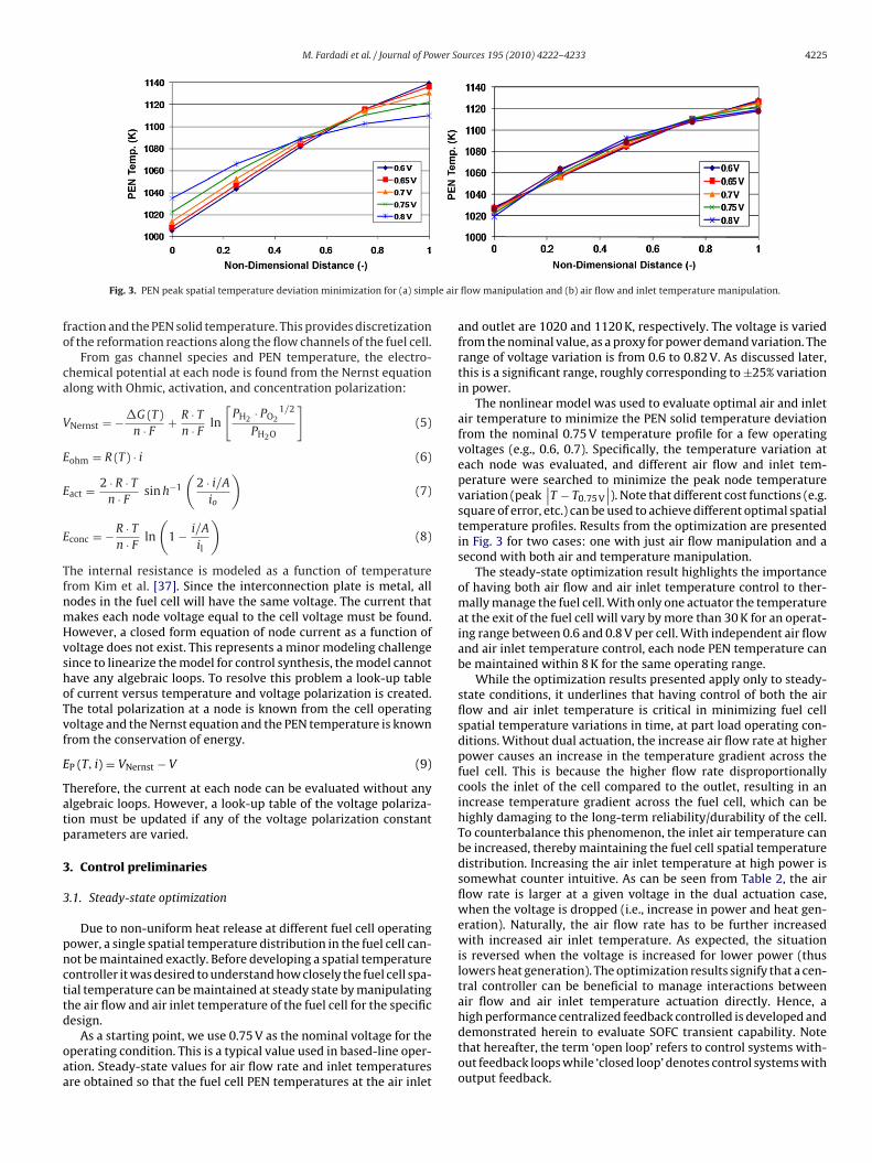
It has been suggested [34] that five nodes is not sufficient toccurately capture the fuel cell spatial temperature distribution.ensitivity analysis of the fuel cell spatial temperature distributionetween a 5 and 10 node model (see Fig. 2) indicates that 5 nodesay result in some inaccuracies in modeling steady-state spatial

emperature distribution. However, it was found that the changen temperature at each node due to perturbation is well captured by5 node model. For example, the PEN spatial temperature response

or a 0.5 V decrease from nominal operating conditions of both theand 10 node model is almost exactly the same (see Fig. 2, right-and side). The results indicate that while 5 nodes cannot preciselyvaluate the temperature profile, a 5 node model can well capturepatial temperature deviation from nominal temperatures for givenerturbation and thus is adequate for evaluating how closely SOFCpatial temperature deviations can be minimized in time. As dis-ussed below, many of the 60 states have weak contributions tohe input–output characteristics of the fuel cell, particularly for theime scales of interest, and can be eliminated without much effect.

.2. Model summary

The fuel cell PEN assembly temperature is resolved one dimen-ionally in the flow direction capturing:

. Heat generation from electrochemistry.

. Conduction heat transfer through the PEN assembly.

. Conduction heat transfer through the metal interconnect.

. Conduction heat transfer between the PEN and metal intercon-nect

. Convection heat transfer to the fuel and air stream.

nsitivity analysis.

6. Surface steam reformation and water gas shift chemical reac-tions.

Conduction heat transfer between the PEN and interconnectplate as well as along the flow direction is modeled by Fourierlaw. Convective heat transfer between the solids and gas flow aremodeled by Newton’s law using constant Nusselt number approx-imation. (See Table 1 for model parameters used e.g., kplate, kpen.)Corresponding energy conservation equation within the PEN con-trol volumes is as follows:

�VCdT

dt=

∑Qhx +

∑Qreact − Qelec (1)

Qelec = −(

hf(H2O)(Te) · i

n · F− iV

)(2)

where Qhx is the heat transfer into the control volume, Qreact isthe heat release from the steam reformation and water gas shiftreactions, Qelec is the heat generated by electrochemistry. The inter-connect plate conservation equation is modeled in a similar fashionwithout the reaction and electrochemical contributions.

Energy and species conservation are applied at each gas channelcontrol volumes as follows:

NCvdT

dt= Ninhin − Nouthout +

∑Q (3)

Nd �X

dt= Nin

�Xin − Nout�Xout + �R (4)

Electrochemical reactions are assumed on the surface of the PEN gas

plate

kpen 10 × 10−3 kW m−1 K−1 PEN conduction coefficientkplate 20 × 10−3 kW m−1 K−1 Interconnect plate conduction coefficientNu 4.12 Nusselt numberio 4000 A m−2 Fuel cell exchange current densityil 9000 A m−2 Fuel cell limiting current density

Page 4

M. Fardadi et al. / Journal of Power Sources 195 (2010) 4222–4233 4225

le air

fo

ca

V

E

E

E

TfnmHvshoTvf

E

Tatp

3

3

pncttd

oaa

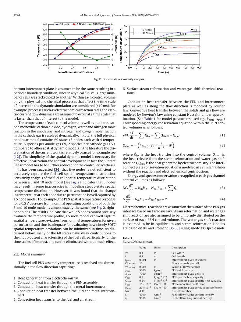
Fig. 3. PEN peak spatial temperature deviation minimization for (a) simp

raction and the PEN solid temperature. This provides discretizationf the reformation reactions along the flow channels of the fuel cell.

From gas channel species and PEN temperature, the electro-hemical potential at each node is found from the Nernst equationlong with Ohmic, activation, and concentration polarization:

Nernst = −�G (T)n · F

+ R · T

n · Fln

[PH2 · PO2

1/2

PH2O

](5)

ohm = R (T) · i (6)

act = 2 · R · T

n · Fsin h−1

(2 · i/A

io

)(7)

conc = −R · T

n · Fln

(1 − i/A

il

)(8)

he internal resistance is modeled as a function of temperaturerom Kim et al. [37]. Since the interconnection plate is metal, allodes in the fuel cell will have the same voltage. The current thatakes each node voltage equal to the cell voltage must be found.owever, a closed form equation of node current as a function ofoltage does not exist. This represents a minor modeling challengeince to linearize the model for control synthesis, the model cannotave any algebraic loops. To resolve this problem a look-up tablef current versus temperature and voltage polarization is created.he total polarization at a node is known from the cell operatingoltage and the Nernst equation and the PEN temperature is knownrom the conservation of energy.

P (T, i) = VNernst − V (9)

herefore, the current at each node can be evaluated without anylgebraic loops. However, a look-up table of the voltage polariza-ion must be updated if any of the voltage polarization constantarameters are varied.

. Control preliminaries

.1. Steady-state optimization

Due to non-uniform heat release at different fuel cell operatingower, a single spatial temperature distribution in the fuel cell can-ot be maintained exactly. Before developing a spatial temperatureontroller it was desired to understand how closely the fuel cell spa-ial temperature can be maintained at steady state by manipulatinghe air flow and air inlet temperature of the fuel cell for the specific

esign.

As a starting point, we use 0.75 V as the nominal voltage for theperating condition. This is a typical value used in based-line oper-tion. Steady-state values for air flow rate and inlet temperaturesre obtained so that the fuel cell PEN temperatures at the air inlet

flow manipulation and (b) air flow and inlet temperature manipulation.

and outlet are 1020 and 1120 K, respectively. The voltage is variedfrom the nominal value, as a proxy for power demand variation. Therange of voltage variation is from 0.6 to 0.82 V. As discussed later,this is a significant range, roughly corresponding to ±25% variationin power.

The nonlinear model was used to evaluate optimal air and inletair temperature to minimize the PEN solid temperature deviationfrom the nominal 0.75 V temperature profile for a few operatingvoltages (e.g., 0.6, 0.7). Specifically, the temperature variation ateach node was evaluated, and different air flow and inlet tem-perature were searched to minimize the peak node temperaturevariation (peak

∣∣T − T0.75 V

∣∣). Note that different cost functions (e.g.square of error, etc.) can be used to achieve different optimal spatialtemperature profiles. Results from the optimization are presentedin Fig. 3 for two cases: one with just air flow manipulation and asecond with both air and temperature manipulation.

The steady-state optimization result highlights the importanceof having both air flow and air inlet temperature control to ther-mally manage the fuel cell. With only one actuator the temperatureat the exit of the fuel cell will vary by more than 30 K for an operat-ing range between 0.6 and 0.8 V per cell. With independent air flowand air inlet temperature control, each node PEN temperature canbe maintained within 8 K for the same operating range.

While the optimization results presented apply only to steady-state conditions, it underlines that having control of both the airflow and air inlet temperature is critical in minimizing fuel cellspatial temperature variations in time, at part load operating con-ditions. Without dual actuation, the increase air flow rate at higherpower causes an increase in the temperature gradient across thefuel cell. This is because the higher flow rate disproportionallycools the inlet of the cell compared to the outlet, resulting in anincrease temperature gradient across the fuel cell, which can behighly damaging to the long-term reliability/durability of the cell.To counterbalance this phenomenon, the inlet air temperature canbe increased, thereby maintaining the fuel cell spatial temperaturedistribution. Increasing the air inlet temperature at high power issomewhat counter intuitive. As can be seen from Table 2, the airflow rate is larger at a given voltage in the dual actuation case,when the voltage is dropped (i.e., increase in power and heat gen-eration). Naturally, the air flow rate has to be further increasedwith increased air inlet temperature. As expected, the situationis reversed when the voltage is increased for lower power (thuslowers heat generation). The optimization results signify that a cen-tral controller can be beneficial to manage interactions betweenair flow and air inlet temperature actuation directly. Hence, a

high performance centralized feedback controlled is developed anddemonstrated herein to evaluate SOFC transient capability. Notethat hereafter, the term ‘open loop’ refers to control systems with-out feedback loops while ‘closed loop’ denotes control systems withoutput feedback.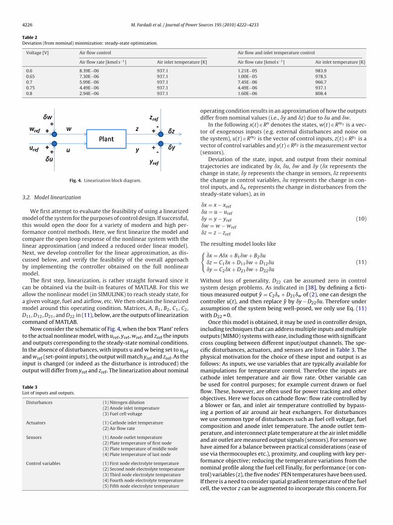

Page 5

4226 M. Fardadi et al. / Journal of Power Sources 195 (2010) 4222–4233

Table 2Deviation (from nominal) minimization: steady-state optimization.

Voltage [V] Air flow control Air flow and inlet temperature control

Air flow rate [kmol s−1] Air inlet temperature [K] Air flow rate [kmol s−1] Air inlet temperature [K]

0.6 8.39E−06 937.1 1.21E−05 983.90.65 7.30E−06 937.10.7 5.99E−06 937.10.75 4.49E−06 937.10.8 2.94E−06 937.1

3

mtfclNcbm

caamDc

taIaio

TL

Fig. 4. Linearization block diagram.

.2. Model linearization

We first attempt to evaluate the feasibility of using a linearizedodel of the system for the purposes of control design. If successful,

his would open the door for a variety of modern and high per-ormance control methods. Here, we first linearize the model andompare the open loop response of the nonlinear system with theinear approximation (and indeed a reduced order linear model).ext, we develop controller for the linear approximation, as dis-ussed below, and verify the feasibility of the overall approachy implementing the controller obtained on the full nonlinearodel.The first step, linearization, is rather straight forward since it

an be obtained via the built-in features of MATLAB. For this wellow the nonlinear model (in SIMULINK) to reach steady state, forgiven voltage, fuel and airflow, etc. We then obtain the linearizedodel around this operating condition. Matrices, A, B1, B2, C1, C2,

11, D12, D21, and D22 in (11), below, are the outputs of linearizationommand of MATLAB.

Now consider the schematic of Fig. 4, when the box ‘Plant’ referso the actual nonlinear model, with uref, yref, wref, and zref the inputsnd outputs corresponding to the steady-state nominal conditions.

n the absence of disturbances, with inputs u and w being set to urefnd wref (set-point inputs), the output will match yref and zref. As thenput is changed (or indeed as the disturbance is introduced) theutput will differ from yref and zref. The linearization about nominal

able 3ist of inputs and outputs.

Disturbances (1) Nitrogen dilution(2) Anode inlet temperature(3) Fuel cell voltage

Actuators (1) Cathode inlet temperature(2) Air flow rate

Sensors (1) Anode outlet temperature(2) Plate temperature of first node(3) Plate temperature of middle node(4) Plate temperature of last node

Control variables (1) First node electrolyte temperature(2) Second node electrolyte temperature(3) Third node electrolyte temperature(4) Fourth node electrolyte temperature(5) Fifth node electrolyte temperature

1.00E−05 978.57.45E−06 966.74.49E−06 937.11.60E−06 808.4

operating condition results in an approximation of how the outputsdiffer from nominal values (i.e., ıy and ız) due to ıu and ıw.

In the following x(t) ∈ Rn denotes the states, w(t) ∈ Rm1 is a vec-tor of exogenous inputs (e.g. external disturbances and noise onthe system), u(t) ∈ Rm2 is the vector of control inputs, z(t) ∈ Rp1 is avector of control variables and y(t) ∈ Rp2 is the measurement vector(sensors).

Deviation of the state, input, and output from their nominaltrajectories are indicated by ıx, ıu, ıw and ıy (ıx represents thechange in state, ıy represents the change in sensors, ız representsthe change in control variables, ıu represents the change in con-trol inputs, and ıw represents the change in disturbances from thesteady-state values), as in

ıx = x − xrefıu = u − urefıy = y − yrefıw = w − wrefız = z − zref

(10)

The resulting model looks like{ıx = Aıx + B1ıw + B2ıuız = C1ıx + D11ıw + D12ıuıy = C2ıx + D21ıw + D22ıu

(11)

Without loss of generality, D22 can be assumed zero in controlsystem design problems. As indicated in [38], by defining a ficti-tious measured output y = C2ıx + D21ıw of (2), one can design thecontroller u(t), and then replace y by ıy − D22ıu. Therefore underassumption of the system being well-posed, we only use Eq. (11)with D22 = 0.

Once this model is obtained, it may be used in controller design,including techniques that can address multiple inputs and multipleoutputs (MIMO) systems with ease, including those with significantcross coupling between different input/output channels. The spe-cific disturbances, actuators, and sensors are listed in Table 3. Thephysical motivation for the choice of these input and output is asfollows: As inputs, we use variables that are typically available formanipulations for temperature control. Therefore the inputs arecathode inlet temperature and air flow rate. Other variable canbe used for control purposes; for example current drawn or fuelflow. These, however, are often used for power tracking and otherobjectives. Here we focus on cathode flow: flow rate controlled bya blower or fan, and inlet air temperature controlled by bypass-ing a portion of air around air heat exchangers. For disturbanceswe use common type of disturbances such as fuel cell voltage, fuelcomposition and anode inlet temperature. The anode outlet tem-perature, and interconnect plate temperature at the air inlet middleand air outlet are measured output signals (sensors). For sensors wehave aimed for a balance between practical considerations (ease ofuse via thermocouples etc.), proximity, and coupling with key per-

formance objective; reducing the temperature variations from thenominal profile along the fuel cell Finally, for performance (or con-trol) variables (z), the five nodes’ PEN temperatures have been used.If there is a need to consider spatial gradient temperature of the fuelcell, the vector z can be augmented to incorporate this concern. For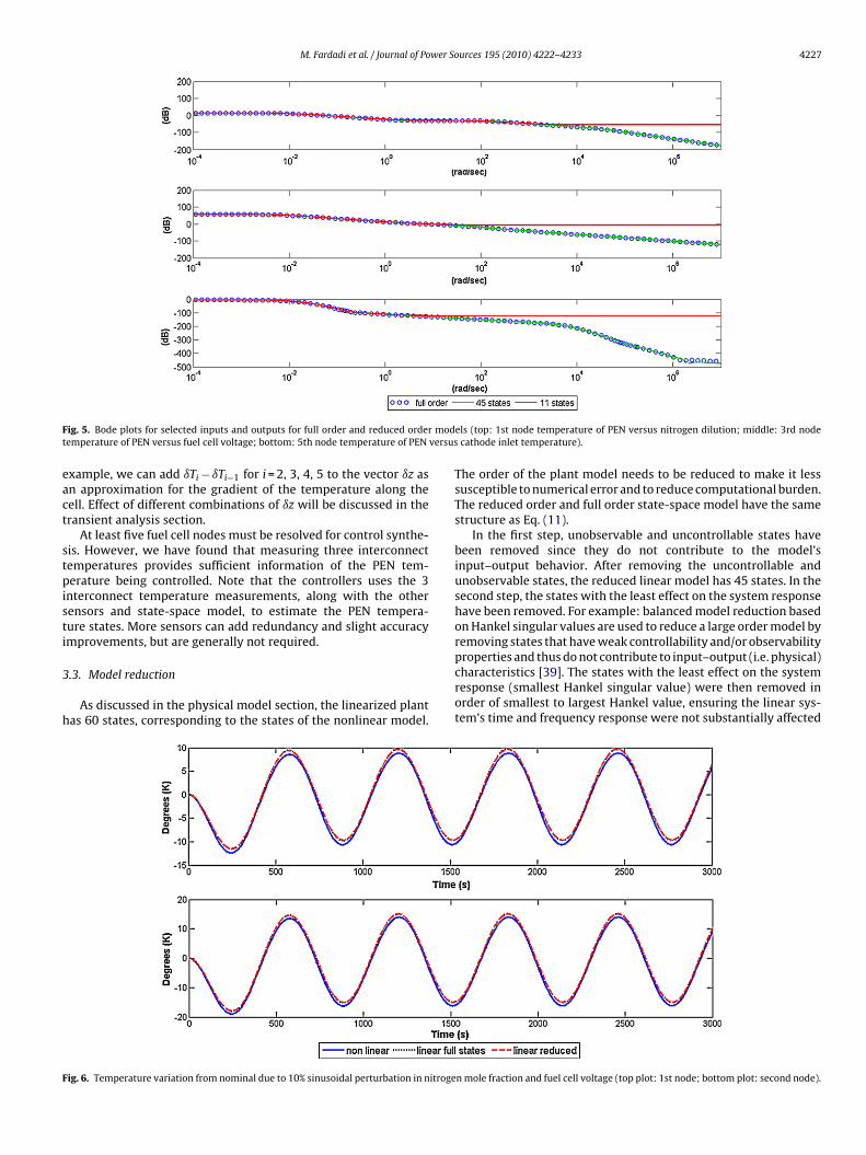

Page 6

M. Fardadi et al. / Journal of Power Sources 195 (2010) 4222–4233 4227

F modt versus

eact

stpisti

3

h

F

ig. 5. Bode plots for selected inputs and outputs for full order and reduced orderemperature of PEN versus fuel cell voltage; bottom: 5th node temperature of PEN

xample, we can add ıTi − ıTi−1 for i = 2, 3, 4, 5 to the vector ız asn approximation for the gradient of the temperature along theell. Effect of different combinations of ız will be discussed in theransient analysis section.

At least five fuel cell nodes must be resolved for control synthe-is. However, we have found that measuring three interconnectemperatures provides sufficient information of the PEN tem-erature being controlled. Note that the controllers uses the 3

nterconnect temperature measurements, along with the otherensors and state-space model, to estimate the PEN tempera-ure states. More sensors can add redundancy and slight accuracymprovements, but are generally not required.

.3. Model reduction

As discussed in the physical model section, the linearized plantas 60 states, corresponding to the states of the nonlinear model.

ig. 6. Temperature variation from nominal due to 10% sinusoidal perturbation in nitroge

els (top: 1st node temperature of PEN versus nitrogen dilution; middle: 3rd nodecathode inlet temperature).

The order of the plant model needs to be reduced to make it lesssusceptible to numerical error and to reduce computational burden.The reduced order and full order state-space model have the samestructure as Eq. (11).

In the first step, unobservable and uncontrollable states havebeen removed since they do not contribute to the model’sinput–output behavior. After removing the uncontrollable andunobservable states, the reduced linear model has 45 states. In thesecond step, the states with the least effect on the system responsehave been removed. For example: balanced model reduction basedon Hankel singular values are used to reduce a large order model byremoving states that have weak controllability and/or observability

properties and thus do not contribute to input–output (i.e. physical)characteristics [39]. The states with the least effect on the systemresponse (smallest Hankel singular value) were then removed inorder of smallest to largest Hankel value, ensuring the linear sys-tem’s time and frequency response were not substantially affected

n mole fraction and fuel cell voltage (top plot: 1st node; bottom plot: second node).

Page 7

4 wer S

aur5m

krembmf

trrotf

mmprtabib

4

cvtTrt

tst{N(t

228 M. Fardadi et al. / Journal of Po

fter each removal. In this system the range of Hankel singular val-es was from very close to zero to 3.97 × 107. Due to a natural, andelatively large, gap in the singular values between about 80 and00, we chose to keep those above 100, leading to a reduced orderodel of order 11.After model reduction, the model contained 11 states with Han-

el singular values greater than 102. Fig. 5 compares the frequencyesponse for the full state linear model and the reduced order lin-ar models (order 45, and 11). The difference between full orderodel and reduced order models is not important after 102 rad s−1,

ecause temperature response is a slow process. Therefore, theodel with 11 states is a good approximation of full order model

or our range of frequency.To further evaluate the effects of linearization and model reduc-

ion, the open loop time response of the full order linear, theeduced order linear and the nonlinear models were compared for aepresentative disturbance. Fig. 6 provides the open loop responsef the linearized model, reduced order model and nonlinear sys-em (actual system) to a 10% sinusoidal variation in nitrogen modelraction and voltage.

Fig. 6 indicates that the response predicted by reduced orderodel matches well the response predicted from the nonlinearodel and that perturbations in fuel cell voltage and fuel com-

osition have a substantial effect on the system’s operating point,equiring control for disturbance rejection. The large variations ofemperature due to load perturbation can lead to thermal fatiguend decrease the life of the fuel cell [13,23]. Note several otherounded disturbances were also tested, all of which lead to sim-

lar results. These results are not shown here for the sake ofrevity.

. Feedback control design

In this section, the concepts and definitions used to designontrollers are presented. Once a linearized model is available, aariety of control methods can be used. Here we present a con-roller obtained from a standard H-infinity or L-2 gain approach.his is partly due to the natural match between our objectives:educing the effects of disturbances on the control outputs, and theemperature profile of the fuel cell [40].

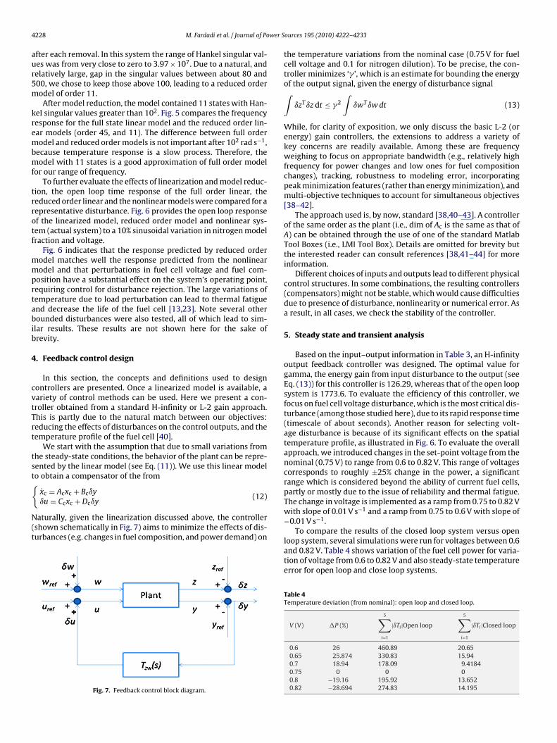
We start with the assumption that due to small variations fromhe steady-state conditions, the behavior of the plant can be repre-ented by the linear model (see Eq. (11)). We use this linear modelo obtain a compensator of the from

xc = Acxc + Bcıy

ıu = Ccxc + Dcıy

(12)

aturally, given the linearization discussed above, the controllershown schematically in Fig. 7) aims to minimize the effects of dis-urbances (e.g. changes in fuel composition, and power demand) on

Fig. 7. Feedback control block diagram.

ources 195 (2010) 4222–4233

the temperature variations from the nominal case (0.75 V for fuelcell voltage and 0.1 for nitrogen dilution). To be precise, the con-troller minimizes ‘� ’, which is an estimate for bounding the energyof the output signal, given the energy of disturbance signal∫

ızT ız dt ≤ �2

∫ıwT ıw dt (13)

While, for clarity of exposition, we only discuss the basic L-2 (orenergy) gain controllers, the extensions to address a variety ofkey concerns are readily available. Among these are frequencyweighing to focus on appropriate bandwidth (e.g., relatively highfrequency for power changes and low ones for fuel compositionchanges), tracking, robustness to modeling error, incorporatingpeak minimization features (rather than energy minimization), andmulti-objective techniques to account for simultaneous objectives[38–42].

The approach used is, by now, standard [38,40–43]. A controllerof the same order as the plant (i.e., dim of Ac is the same as that ofA) can be obtained through the use of one of the standard MatlabTool Boxes (i.e., LMI Tool Box). Details are omitted for brevity butthe interested reader can consult references [38,41–44] for moreinformation.

Different choices of inputs and outputs lead to different physicalcontrol structures. In some combinations, the resulting controllers(compensators) might not be stable, which would cause difficultiesdue to presence of disturbance, nonlinearity or numerical error. Asa result, in all cases, we check the stability of the controller.

5. Steady state and transient analysis

Based on the input–output information in Table 3, an H-infinityoutput feedback controller was designed. The optimal value forgamma, the energy gain from input disturbance to the output (seeEq. (13)) for this controller is 126.29, whereas that of the open loopsystem is 1773.6. To evaluate the efficiency of this controller, wefocus on fuel cell voltage disturbance, which is the most critical dis-turbance (among those studied here), due to its rapid response time(timescale of about seconds). Another reason for selecting volt-age disturbance is because of its significant effects on the spatialtemperature profile, as illustrated in Fig. 6. To evaluate the overallapproach, we introduced changes in the set-point voltage from thenominal (0.75 V) to range from 0.6 to 0.82 V. This range of voltagescorresponds to roughly ±25% change in the power, a significantrange which is considered beyond the ability of current fuel cells,partly or mostly due to the issue of reliability and thermal fatigue.The change in voltage is implemented as a ramp from 0.75 to 0.82 Vwith slope of 0.01 V s−1 and a ramp from 0.75 to 0.6 V with slope of−0.01 V s−1.

To compare the results of the closed loop system versus openloop system, several simulations were run for voltages between 0.6and 0.82 V. Table 4 shows variation of the fuel cell power for varia-tion of voltage from 0.6 to 0.82 V and also steady-state temperatureerror for open loop and close loop systems.

Table 4Temperature deviation (from nominal): open loop and closed loop.

V (V) �P (%)

5∑i=1

|ıTi|Open loop

5∑i=1

|ıTi|Closed loop

0.6 26 460.89 20.650.65 25.874 330.83 15.940.7 18.94 178.09 9.41840.75 0 0 00.8 −19.16 195.92 13.6520.82 −28.694 274.83 14.195

Page 8

M. Fardadi et al. / Journal of Power Sources 195 (2010) 4222–4233 4229

asing

wd

(

5

lndmt

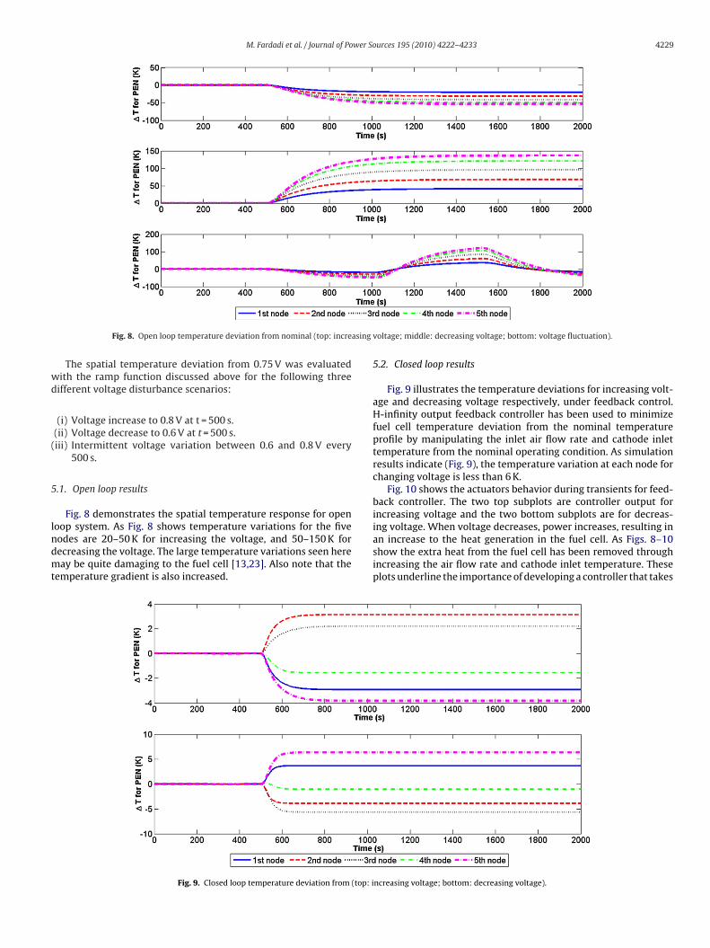
Fig. 8. Open loop temperature deviation from nominal (top: incre

The spatial temperature deviation from 0.75 V was evaluatedith the ramp function discussed above for the following threeifferent voltage disturbance scenarios:

(i) Voltage increase to 0.8 V at t = 500 s.(ii) Voltage decrease to 0.6 V at t = 500 s.iii) Intermittent voltage variation between 0.6 and 0.8 V every

500 s.

.1. Open loop results

Fig. 8 demonstrates the spatial temperature response for open

oop system. As Fig. 8 shows temperature variations for the fiveodes are 20–50 K for increasing the voltage, and 50–150 K forecreasing the voltage. The large temperature variations seen hereay be quite damaging to the fuel cell [13,23]. Also note that the

emperature gradient is also increased.

Fig. 9. Closed loop temperature deviation from (top: i

voltage; middle: decreasing voltage; bottom: voltage fluctuation).

5.2. Closed loop results

Fig. 9 illustrates the temperature deviations for increasing volt-age and decreasing voltage respectively, under feedback control.H-infinity output feedback controller has been used to minimizefuel cell temperature deviation from the nominal temperatureprofile by manipulating the inlet air flow rate and cathode inlettemperature from the nominal operating condition. As simulationresults indicate (Fig. 9), the temperature variation at each node forchanging voltage is less than 6 K.

Fig. 10 shows the actuators behavior during transients for feed-back controller. The two top subplots are controller output forincreasing voltage and the two bottom subplots are for decreas-

ing voltage. When voltage decreases, power increases, resulting inan increase to the heat generation in the fuel cell. As Figs. 8–10show the extra heat from the fuel cell has been removed throughincreasing the air flow rate and cathode inlet temperature. Theseplots underline the importance of developing a controller that takes

ncreasing voltage; bottom: decreasing voltage).

Page 9

4230 M. Fardadi et al. / Journal of Power Sources 195 (2010) 4222–4233

creasi

bttfiwstobattwdoc

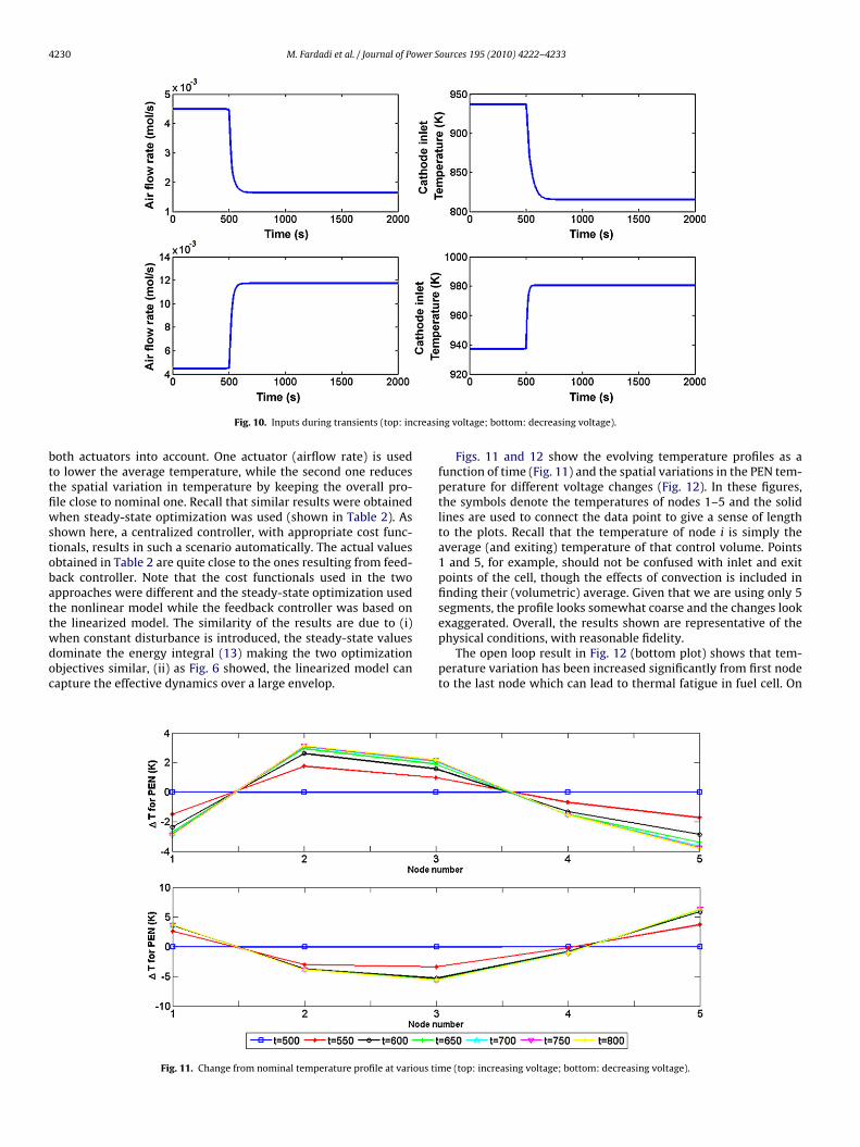
Fig. 10. Inputs during transients (top: in

oth actuators into account. One actuator (airflow rate) is usedo lower the average temperature, while the second one reduceshe spatial variation in temperature by keeping the overall pro-le close to nominal one. Recall that similar results were obtainedhen steady-state optimization was used (shown in Table 2). As

hown here, a centralized controller, with appropriate cost func-ionals, results in such a scenario automatically. The actual valuesbtained in Table 2 are quite close to the ones resulting from feed-ack controller. Note that the cost functionals used in the twopproaches were different and the steady-state optimization usedhe nonlinear model while the feedback controller was based onhe linearized model. The similarity of the results are due to (i)

hen constant disturbance is introduced, the steady-state valuesominate the energy integral (13) making the two optimizationbjectives similar, (ii) as Fig. 6 showed, the linearized model canapture the effective dynamics over a large envelop.

Fig. 11. Change from nominal temperature profile at various tim

ng voltage; bottom: decreasing voltage).

Figs. 11 and 12 show the evolving temperature profiles as afunction of time (Fig. 11) and the spatial variations in the PEN tem-perature for different voltage changes (Fig. 12). In these figures,the symbols denote the temperatures of nodes 1–5 and the solidlines are used to connect the data point to give a sense of lengthto the plots. Recall that the temperature of node i is simply theaverage (and exiting) temperature of that control volume. Points1 and 5, for example, should not be confused with inlet and exitpoints of the cell, though the effects of convection is included infinding their (volumetric) average. Given that we are using only 5segments, the profile looks somewhat coarse and the changes lookexaggerated. Overall, the results shown are representative of the

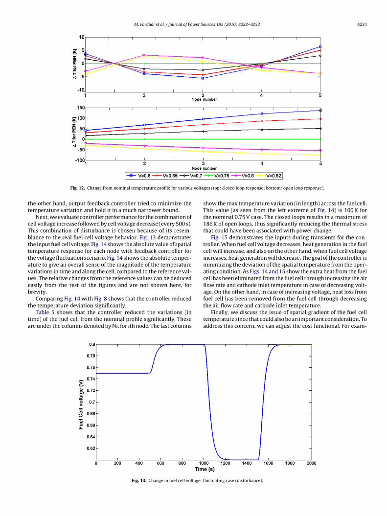
physical conditions, with reasonable fidelity.

The open loop result in Fig. 12 (bottom plot) shows that tem-perature variation has been increased significantly from first nodeto the last node which can lead to thermal fatigue in fuel cell. On

e (top: increasing voltage; bottom: decreasing voltage).

Page 10

M. Fardadi et al. / Journal of Power Sources 195 (2010) 4222–4233 4231

volta

tt

cTbtttavueb

t

ta

Fig. 12. Change from nominal temperature profile for various

he other hand, output feedback controller tried to minimize theemperature variation and hold it in a much narrower bound.

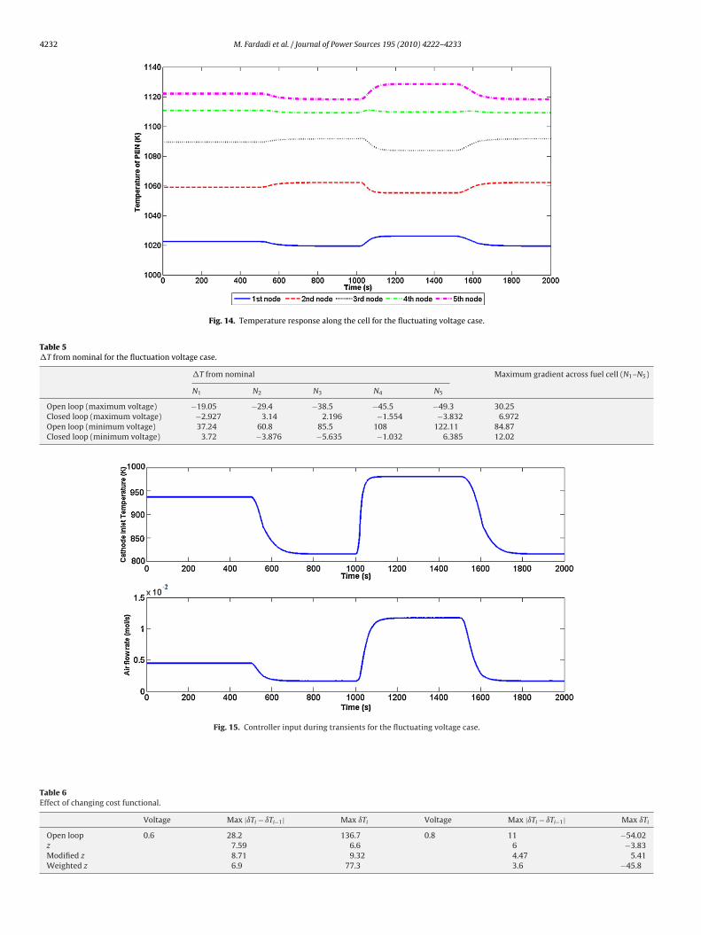
Next, we evaluate controller performance for the combination ofell voltage increase followed by cell voltage decrease (every 500 s).his combination of disturbance is chosen because of its resem-lance to the real fuel cell voltage behavior. Fig. 13 demonstrateshe input fuel cell voltage. Fig. 14 shows the absolute value of spatialemperature response for each node with feedback controller forhe voltage fluctuation scenario. Fig. 14 shows the absolute temper-ture to give an overall sense of the magnitude of the temperatureariations in time and along the cell, compared to the reference val-es. The relative changes from the reference values can be deducedasily from the rest of the figures and are not shown here, forrevity.

Comparing Fig. 14 with Fig. 8 shows that the controller reduced

he temperature deviation significantly.

Table 5 shows that the controller reduced the variations (inime) of the fuel cell from the nominal profile significantly. Thesere under the columns denoted by Ni, for ith node. The last columns

Fig. 13. Change in fuel cell voltage:

ges (top: closed loop response; bottom: open loop response).

show the max temperature variation (in length) across the fuel cell.This value (as seen from the left extreme of Fig. 14) is 100 K forthe nominal 0.75 V case. The closed loops results in a maximum of186 K of open loops, thus significantly reducing the thermal stressthat could have been associated with power change.

Fig. 15 demonstrates the inputs during transients for the con-troller. When fuel cell voltage decreases, heat generation in the fuelcell will increase, and also on the other hand, when fuel cell voltageincreases, heat generation will decrease. The goal of the controller isminimizing the deviation of the spatial temperature from the oper-ating condition. As Figs. 14 and 15 show the extra heat from the fuelcell has been eliminated from the fuel cell through increasing the airflow rate and cathode inlet temperature in case of decreasing volt-age. On the other hand, in case of increasing voltage, heat loss fromfuel cell has been removed from the fuel cell through decreasing

the air flow rate and cathode inlet temperature.

Finally, we discuss the issue of spatial gradient of the fuel celltemperature since that could also be an important consideration. Toaddress this concern, we can adjust the cost functional. For exam-

fluctuating case (disturbance).

Page 11

4232 M. Fardadi et al. / Journal of Power Sources 195 (2010) 4222–4233

Fig. 14. Temperature response along the cell for the fluctuating voltage case.

Table 5�T from nominal for the fluctuation voltage case.

�T from nominal Maximum gradient across fuel cell (N1–N5)

N1 N2 N3 N4 N5

Open loop (maximum voltage) −19.05 −29.4 −38.5 −45.5 −49.3 30.25Closed loop (maximum voltage) −2.927 3.14 2.196 −1.554 −3.832 6.972Open loop (minimum voltage) 37.24 60.8 85.5 108 122.11 84.87Closed loop (minimum voltage) 3.72 −3.876 −5.635 −1.032 6.385 12.02

Fig. 15. Controller input during transients for the fluctuating voltage case.

Table 6Effect of changing cost functional.

Voltage Max |ıTi − ıTi−1| Max ıTi Voltage Max |ıTi − ıTi−1| Max ıTi

Open loop 0.6 28.2 136.7 0.8 11 −54.02z 7.59 6.6 6 −3.83Modified z 8.71 9.32 4.47 5.41Weighted z 6.9 77.3 3.6 −45.8

Page 12

wer So

potrzTtii

foi‘asasdamc

6

mesttSrbocidctoattp

R

[

[

[

[

[[

[

[

[

[

[[

[

[

[

[

[

[

[

[

[

[

[

[

[[[[

[[[

[

M. Fardadi et al. / Journal of Po

le, we can add ıTi − ıTi−1 for i = 2,3,4,5 to the control/performanceutput vector (i.e., z) as an approximation for the gradient of theemperature along the cell. The results are listed in Table 6. Theow ‘z’ corresponds to the ız vector used so far. The row ‘modified’ corresponds to the case of having the four ıTi − ıTi−1 plus ıT4.he last entry, ıT4, is to hold the overall temperature profile closeo the nominal and prevent large drifts. ‘Weighted z’ in the last rows similar to the ‘new z’ case, except the entry corresponding to ıT4s multiplied by 0.1 to place more emphasis on the slope reductions.

The results of Table 6 show that this modification to the costunctional can be used to reduce the peak (or worst case) slopef the temperature along the cell, if that is desired. There is onenconsistency in Table 6, for decreasing fuel cell voltage in theModified z’ versus ‘z’. Given that the controller here is aimedt reducing the energy (i.e., integral of the square) of the signal,uch anomalies can occur. With modest modifications, one canttempt energy to peak or peak-to-peak minimization, but we leaveuch variations to future work. The exact level of trade-off in theesign iterations depends on the specific properties of the fuel cellnd is beyond the scope of this paper. It suffices to say that theethodology presented is flexible enough to accommodate such

oncerns.

. Conclusion

Controlling SOFC spatial temperature plays an important role ininimizing fuel cell thermal stresses and fatigue. Dynamic mod-

ling has been used to design and evaluate controls in reducingignificantly fuel cell spatial temperature variation during loadransients. Dynamic modeling provides an effective means to inves-igate controls without risking loss or deterioration of expensiveOFC systems. The actuation is through manipulating the air flowate and cathode inlet temperature. The control technique is aasic H-infinity output feedback design, developed for a reduce-rder linearized model of the fuel cell, around a baseline operatingondition. This control technique is shown to be quite effectiven reducing the thermal variations, due to changes in the poweremand, while a variety of other disturbances (e.g., fuel variations)an easily be addressed but are left to future work. Similarly sys-ematic approaches aimed at reducing peak response (e.g., errorr variations) to peak or energy bounded disturbance can also bettempted with relative ease. Simulated control results indicate forhe first time that future SOFC systems can be designed and con-rolled to have superb load following characteristic with less thanreviously expected thermal stresses.

eferences

[1] S. Chalk, American Recovery and Reinvestment Act Program Plan for the Officeof Energy Efficiency and Renewable Energy, Department of Energy, The Officeof Energy Efficiency and Renewable Energy (EERE), 2009.

[2] E. Sison-Lebrilla, G. Kibrya, V. Tiangco, D. Yen, P. Sethi, M. Kane, Research Devel-opment and Demonstration Roadmap, California Energy Commission PIERRenewable Energy Technologies Program, CEC-500-2007-035, Sacremento,2007, 45 pp.

[3] A. Cano, F. Jurado, Optimum Location of Biomass-Fuelled Gas Turbines in AnElectric System, 2006, 6 pp.

[4] F. Mueller, F. Jabbari, R. Gaynor, J. Brouwer, Journal of Power Sources 172 (1)(2007) 308–323.

[5] F. Mueller, R. Gaynor, A.E. Auld, J. Brouwer, F. Jabbari, G.S. Samuelsen, Journalof Power Sources 176 (1) (2008) 229–239.

[

[

[

urces 195 (2010) 4222–4233 4233

[6] F. Mueller, Journal of Power Sources 187 (2) (2009) 452–460.[7] F. Mueller, B. Tarroja, J. Maclay, F. Jabbari, J. Brouwer, S. Samuelsen, Design, Sim-

ulation and Control of a 100 Megawatt Class Solid Oxide Fuel Cell Gas TurbineHybrid System, ASME, Denver, Colorado, 2008.

[8] F. Mueller, The Dynamics and Control of Integrated Solid Oxide Fuel Cell Sys-tems: Transient Load-Following and Fuel Disturbance Rejection, University ofCalifornia, Irvine, Irvine, 2008 (Doctorate).

[9] A.M. Murshed, B. Huang, K. Nandakumar, Estimation and control of solid oxidefuel cell system, Computers and Chemical Engineering 34 (2010) 96–111.

10] M.C. Williams, J.P. Strakey, W.A. Surdoval, L.C. Wilson, Solid State Ionics 177(19–25) (2006) 2039–2044.

11] M.F. Serincan, U. Pasaogullari, N.M. Sammes, A transient analysis of a microtubular solid oxide fuel cell (SOFC), Journal of Power Sources 194 (2009)864–872.

12] A. Nakajo, C. Stiller, G. Harkegard, O. Bolland, Journal of Power Sources 158 (1)(2006) 287–294.

13] A. Nakajo, Z. Wuillemin, J. Van herle, D. Favrat, Journal of Power Sources 193(1) (2009) 203–215.

14] Y.C. Hsiao, J.R. Selman, Solid State Ionics 98 (1–2) (1997) 33–38.15] F. Mueller, F. Jabbari, J. Brouwer, R. Roberts, T. Junker, H. Ghezel-Ayagh, Journal

of Fuel Cell Science and Technology 4 (2007) 221–230.16] C. Stiller, B. Thorud, O. Bolland, R. Kandepu, L. Imsland, Journal of Power Sources

158 (1) (2006) 303–315.17] R. Gaynor, F. Mueller, F. Jabbari, J. Brouwer, Journal of Power Sources 180 (1)

(2008) 330–342.18] B.A. Haberman, J.B. Young, International Journal of Heat and Mass Transfer 48

(25–26) (2005) 5475–5487.19] H.-K. Park, Y.-R. Lee, M.-H. Kim, G.-Y. Chung, S.-W. Nam, S.-A. Hong, T.-H. Lim,

H.-C. Lim, Journal of Power Sources 104 (1) (2002) 140–147.20] P.-W. Li, M.K. Chyu, Journal of Power Sources 124 (2) (2003) 487–498.21] J. Yang, X. Li, H.-G. Mou, L. Jian, Journal of Power Sources 193 (2) (2009) 699–

705.22] J. Yang, X. Li, H.-G. Mou, L. Jian, Journal of Power Sources 188 (2) (2009) 475–

482.23] A. Nakajo, Z. Wuillemin, J. Van herle, D. Favrat, Journal of Power Sources 193

(1) (2009) 216–226.24] Y. Inui, N. Ito, T. Nakajima, A. Urata, Energy Conversion and Management 47

(15–16) (2006) 2319–2328.25] R. Roberts, J. Brouwer, F. Jabbari, T. Junker, H. Ghezel-Ayagh, Journal of Power

Sources 161 (1) (2006) 484–491.26] Y. Kuniba, Development and Analysis of Load Following SOFC/GT Hybrid Sys-

tem Control Strategies for Commercial Building Applications, University ofCalifornia, Irvine, Irvine, 2007.

27] T. Kaneko, J. Brouwer, G.S. Samuelsen, Journal of Power Sources 160 (1) (2006)316–325.

28] J. Brouwer, F. Jabbari, E.M. Leal, T. Orr, Journal of Power Sources 158 (1) (2006)213–224.

29] K. Min, J. Brouwer, J. Auckland, F. Mueller, S. Samuelsen, Dynamic Simulationof a Stationary PEM Fuel Cell System, ASME, Irvine, CA, 2006.

30] F. Mueller, J. Brouwer, F. Jabbari, S. Samuelsen, Dynamic Simulation of an Inte-grated Solid Oxide Fuel Cell System Including Current-Based-Fuel Control, 2005May 23–25, ASME, Ypsilanti, MI, 2005, pp. 1–11.

31] F. Mueller, J. Brouwer, S. Kang, H.-S. Kim, K. Min, Journal of Power Sources 163(2) (2007) 814–829.

32] R. Roberts, A Dynamic Fuel Cell-Gas Turbine Hybrid Simulation Methodolgy toEstablish Control Strategies and an Improved Ballance of Plant, University ofCalifornia, Irvine, Irvine, 2005, 338 pp. (Doctorate).

33] R. Roberts, J. Brouwer, Journal of Fuel Cell Science and Technology 3 (1) (2006)18–25.

34] S. Campanari, P. Iora, Journal of Power Sources 132 (1–2) (2004) 113–126.35] J. Xu, G.F. Froment, AIChE Journal 35 (1) (1989) 88–96.36] J. Xu, G.F. Froment, AIChE Journal 35 (1) (1989) 97–103.37] J.-W. Kim, A. Virkar, K.-Z. Fung, M. Karum, S. Singhal, Journal of The Electro-

chemistry Society 146 (1) (1999) 69–78.38] T. Iwasaki, R.E. Skelton, Automatica 30 (8) (1994) 1307–1317.39] K. Zhou, J.C. Doyle, Essentials of Robust Control, Prentice Hall, 1998.40] S. Boyd, L.E. Ghaoui, E. Feron, V. Balakrishnan, Linear Matrix Inequalities in

System and Control Theory, 1994.41] P. Gahinet, P. Apkarian, International Journal of Robust and Nonlinear Control

4 (4) (1994) 421–448.

42] C. Scherer, P. Gahinet, M. Chilali, IEEE Transaction on Automatic Control 42 (7)

(1997) 896–911.43] R.E. Skelton, T. Iwaskai, K. Grigoriadis, A Unified Algebraic Approach to Linear

Control Design, Taylor and Francis, London, 1998.44] P. Gahinet, A. Nemirovski, A.J. Laub, M. Chilali, LMI Control Toolbox for Use with

Matlab, The MathWorks, Inc., 1995.