ESE319 Introduction to Microelectronics 1 2008 Kenneth R. Laker (based on P. V. Lopresti 2006) updated 29Oct08 KRL Feedback Basics ● Stability ● Feedback concept ● Feedback in emitter follower ● One-pole feedback and root locus ● Frequency dependent feedback and root locus ● Gain and phase margins ● Conditions for closed loop stability ● Frequency compensation

Welcome message from author
This document is posted to help you gain knowledge. Please leave a comment to let me know what you think about it! Share it to your friends and learn new things together.
Transcript
ESE319 Introduction to Microelectronics
12008 Kenneth R. Laker (based on P. V. Lopresti 2006) updated 29Oct08 KRL
Feedback Basics● Stability● Feedback concept● Feedback in emitter follower● One-pole feedback and root locus● Frequency dependent feedback and root locus● Gain and phase margins● Conditions for closed loop stability● Frequency compensation
ESE319 Introduction to Microelectronics
22008 Kenneth R. Laker (based on P. V. Lopresti 2006) updated 29Oct08 KRL

ESE319 Introduction to Microelectronics
32008 Kenneth R. Laker (based on P. V. Lopresti 2006) updated 29Oct08 KRL
F
F
F
F
F
F
Operational Amplifier From Another View

ESE319 Introduction to Microelectronics
42008 Kenneth R. Laker (based on P. V. Lopresti 2006) updated 29Oct08 KRL
Feedback Block Diagram Point of View
A
β
-+vi vo
vo=A
1AFvi
Fundamental feedback equation
Fundamental block diagram We can split the idealop amp and resistivedivider into 2 separateblocks because theydo not interact with, or“load,” each other.
1. The op amp output isan ideal voltage source.
2. The op amp input draws no current.
F
vf

ESE319 Introduction to Microelectronics
52008 Kenneth R. Laker (based on P. V. Lopresti 2006) updated 29Oct08 KRL
Comments on the Feedback Equation
G=vovi= A1A F
The quantity ' loop-gain and G = closed-loop gain.
AF≫1(and the system is stable – a topic to be discussed later!) the closed-loop gain approximates &and is independent of “A” !
AF
1/F
The quantity A = open-loop gain and = feedback gain.
If the loop gain is much greater than one, i.e.
F
A=vovi
A
β
-+vi vo
F
vf
F=v fvo
G=vovi≈1F
|v f=0
ESE319 Introduction to Microelectronics
62008 Kenneth R. Laker (based on P. V. Lopresti 2006) updated 29Oct08 KRL
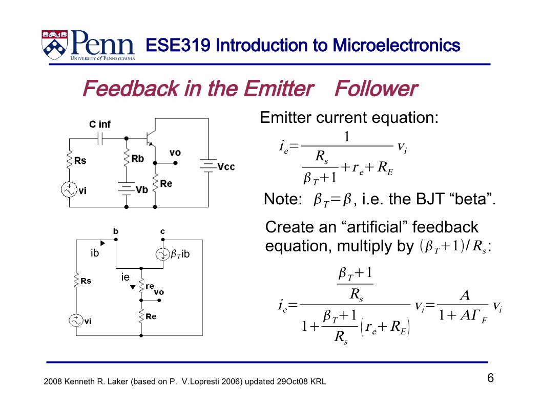
Feedback in the Emitter FollowerEmitter current equation:
ie=1
RsT1
r eREvi
Create an “artificial” feedbackequation, multiply by :
ie=
T1Rs
1T1Rs
r eRE vi=
A1AF
vi
T1/Rs
Note: , i.e. the BJT “beta”. T=
ib
ie
T ib
ESE319 Introduction to Microelectronics
72008 Kenneth R. Laker (based on P. V. Lopresti 2006) updated 29Oct08 KRL
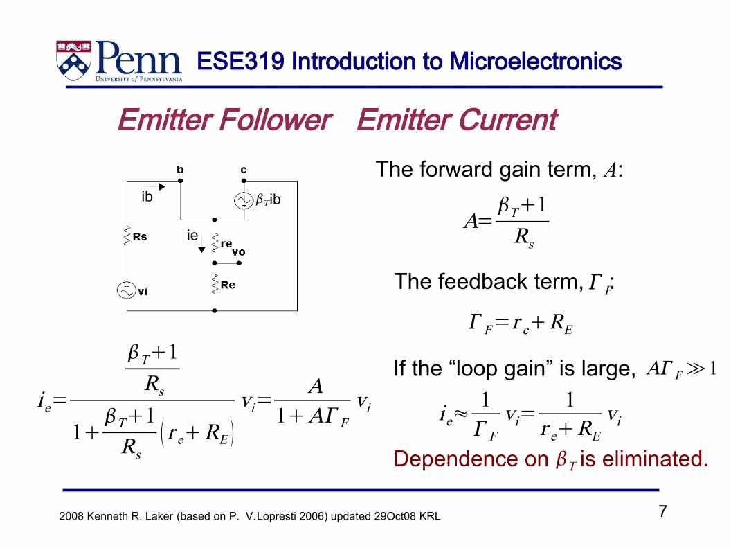
Emitter Follower Emitter Current
ie=
T1Rs
1T1Rs
r eRE vi=
A1AF
vi
The forward gain term, A:
A=T1Rs
The feedback term, :
F=r eRE
If the “loop gain” is large,
ie≈1 Fvi=
1r eRE
vi
F
AF≫1
ib ib
ie
T
Dependence on is eliminated.T

ESE319 Introduction to Microelectronics
82008 Kenneth R. Laker (based on P. V. Lopresti 2006) updated 29Oct08 KRL
Loop Gain Sensitivities For:Forward gain:dGdA
=1
1A F 2
dGG
=1
1A F 21AFA
dA
11AF
dAA
0
Feedback gain:dGd F
=−A2
1A F 2
dGG
=−A2
1AF 21AFA
d F
−A F
1A F d F F
−d F
F
High loop gain makes system insensitive to A, but sensitive to !
G= A1AF
F
==AF∞
AF∞

ESE319 Introduction to Microelectronics
92008 Kenneth R. Laker (based on P. V. Lopresti 2006) updated 29Oct08 KRL
Feedback - One-pole A(s)
Consider the case where:
As=a K0
sa
A
β
-+vi vov
f
F
G=vovi=
A1AF
G s ,F =
a K0
sa
1a F K01sa
=a K0
sa 1F K0
open-loop pole
closed-loop pole
Where and K0 are positive real quantities.F
X-a
j
s= j
F=0
∞F
Root Locus Plot for G s ,F
stable for all ΓF!

ESE319 Introduction to Microelectronics
102008 Kenneth R. Laker (based on P. V. Lopresti 2006) updated 29Oct08 KRL
Feedback - One-pole A(s) cont.As=
a K0
saG s=
a K 0
sa 1F K0=N sD s
GBWOL=GBWCL=a K0
a
Kω
Gain - dB
- 20 dB/dec
20 log10K0
1F K0
a 1F K00
- 20 dB/dec
20 log10K0
frequency (ω)
open-loop (OL) closed-loop (CL)
ESE319 Introduction to Microelectronics
112008 Kenneth R. Laker (based on P. V. Lopresti 2006) updated 29Oct08 KRL
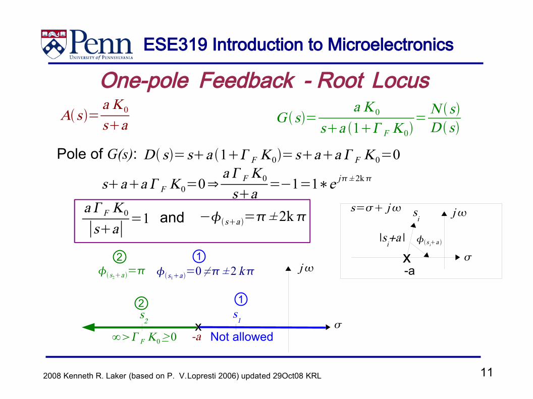
One-pole Feedback - Root LocusG s=
a K 0
sa 1F K0= N sD s
As=a K0
sa
D s=sa 1F K0=saa F K0=0Pole of G(s):
saa F K0=0⇒a F K0
sa=−1=1∗e j± 2k
a F K0
∣sa∣=1 −sa =± 2kand
x
si
|si+a |
-a
s ia
-ax
12
s1a =0≠± 2 k1
s2a =2
∞F K0≥ 0 Not allowed
s1s
2
j
js= j
ESE319 Introduction to Microelectronics
122008 Kenneth R. Laker (based on P. V. Lopresti 2006) updated 29Oct08 KRL
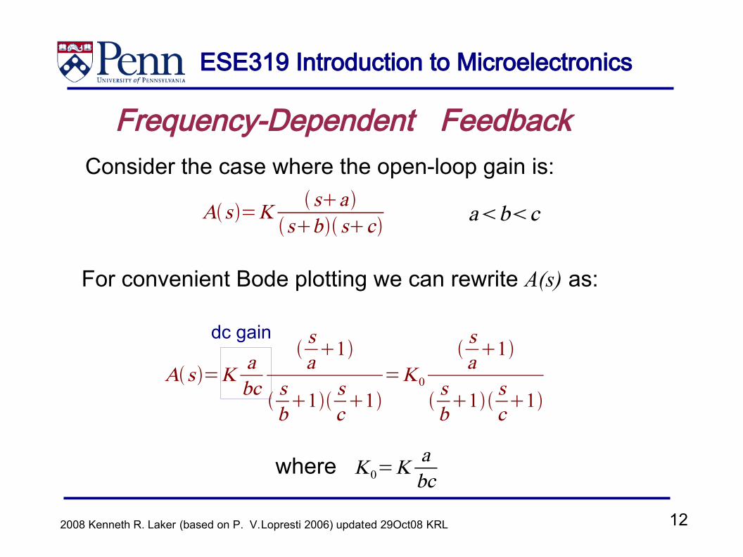
Frequency-Dependent FeedbackConsider the case where the open-loop gain is:
As=K sa sb sc
For convenient Bode plotting we can rewrite A(s) as:
As=K abc
sa1
sb1sc1
=K0
sa1
sb1sc1
abc
K0=Kabc
where
dc gain
ESE319 Introduction to Microelectronics
132008 Kenneth R. Laker (based on P. V. Lopresti 2006) updated 29Oct08 KRL
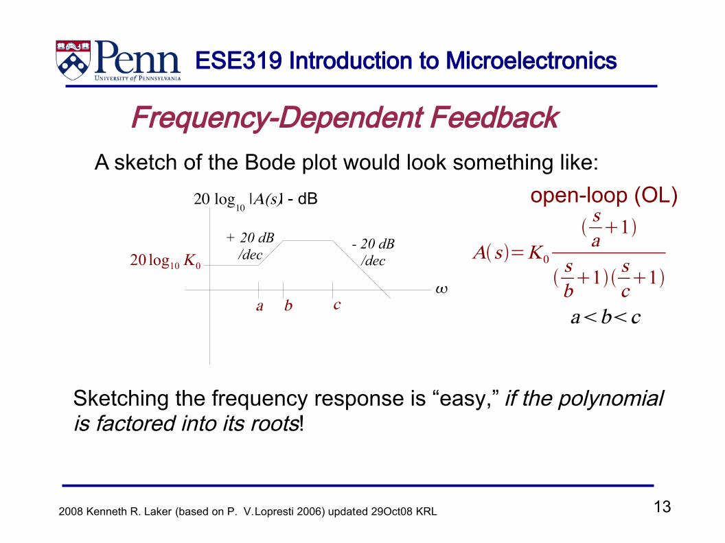
Frequency-Dependent FeedbackA sketch of the Bode plot would look something like:
Sketching the frequency response is “easy,” if the polynomialis factored into its roots!
As=K0
sa1
sb1 s
c1
abca b c
Kω
20 log10
|A(s)| - dB
+ 20 dB/dec
- 20 dB/dec
open-loop (OL)
20 log10K0
ESE319 Introduction to Microelectronics
142008 Kenneth R. Laker (based on P. V. Lopresti 2006) updated 29Oct08 KRL
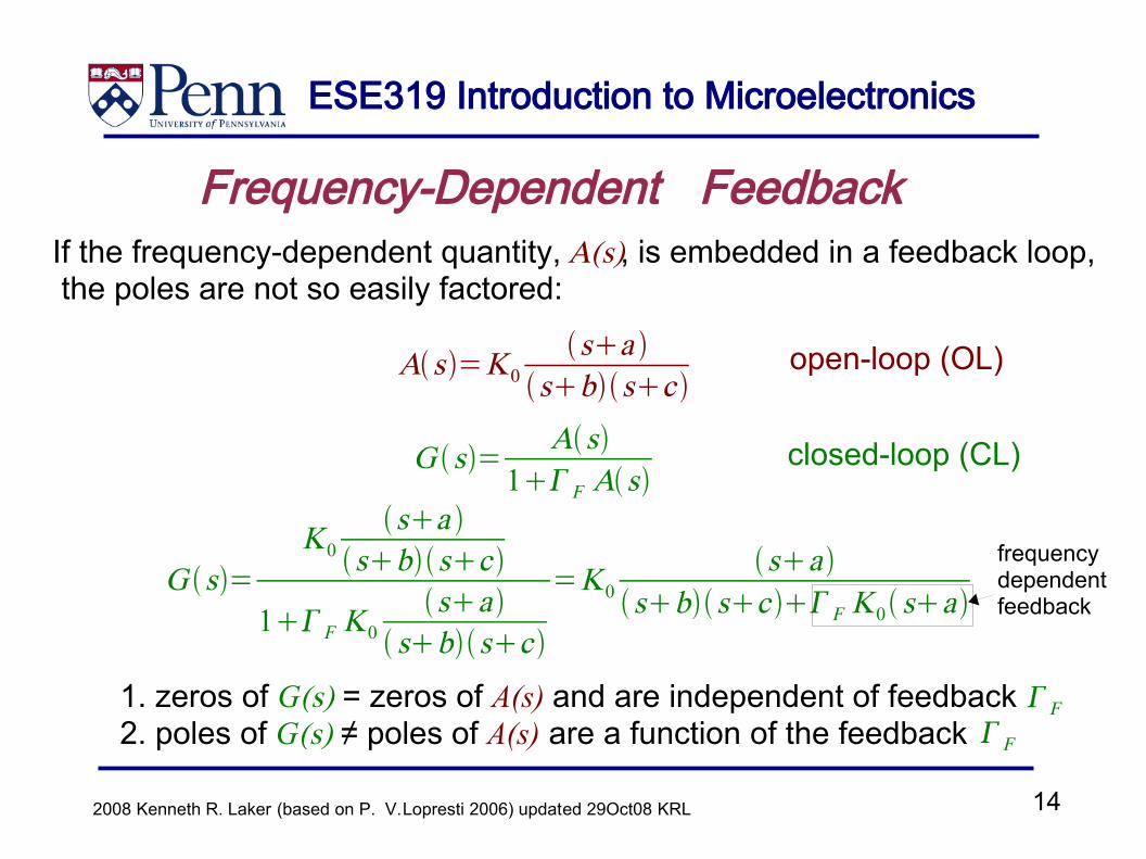
Frequency-Dependent FeedbackIf the frequency-dependent quantity, A(s), is embedded in a feedback loop, the poles are not so easily factored:
As=K0sa
sbsc
G s= As1 F As
G s=K0
sa sbsc
1F K0sa
sbsc
=K0sa
sbsc F K0 sa
open-loop (OL)
closed-loop (CL)
1. zeros of G(s) = zeros of A(s) and are independent of feedback2. poles of G(s) ≠ poles of A(s) are a function of the feedback F
F
frequency dependent feedback
ESE319 Introduction to Microelectronics
152008 Kenneth R. Laker (based on P. V. Lopresti 2006) updated 29Oct08 KRL
Frequency-Dependent Feedback – Root Locus
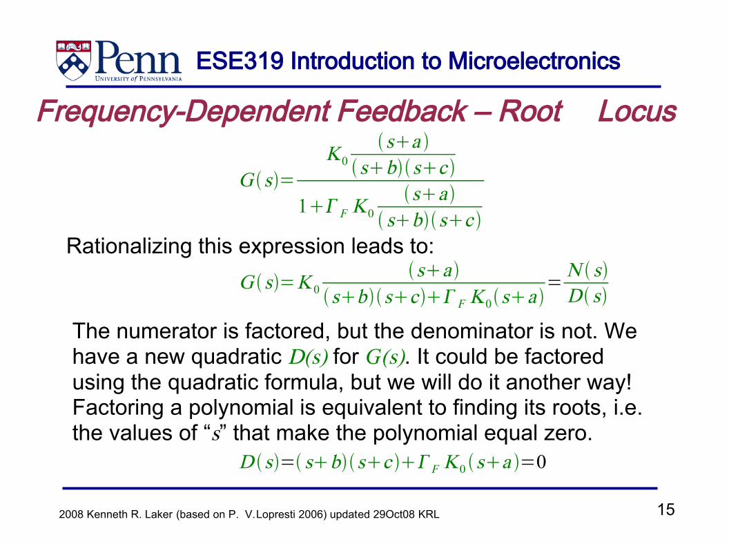
Rationalizing this expression leads to:G s=K 0
sa sbscF K0sa
=N sD s
The numerator is factored, but the denominator is not. Wehave a new quadratic D(s) for G(s). It could be factoredusing the quadratic formula, but we will do it another way!Factoring a polynomial is equivalent to finding its roots, i.e.the values of “s” that make the polynomial equal zero.
D s= sbsc F K0 sa =0
G s=K0
sa sbsc
1F K0sa
sbsc
ESE319 Introduction to Microelectronics
162008 Kenneth R. Laker (based on P. V. Lopresti 2006) updated 29Oct08 KRL
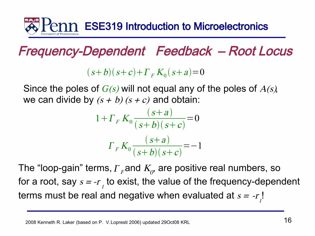
Frequency-Dependent Feedback – Root LocussbscF K0 sa =0
Since the poles of G(s) will not equal any of the poles of A(s), we can divide by (s + b) (s + c) and obtain:
1F K0sa
sbsc=0
The “loop-gain” terms, and K0, are positive real numbers, sofor a root, say s = -r
1 to exist, the value of the frequency-dependent
terms must be real and negative when evaluated at s = -r1!
F K0 sa
sbsc=−1
F

ESE319 Introduction to Microelectronics
172008 Kenneth R. Laker (based on P. V. Lopresti 2006) updated 29Oct08 KRL
Frequency-Dependent Feedback – Root Locus
F K0 sa
sbsc=−1=1∗e j±2k
Working with the complex numbers in polar form:
F K0∣sa∣
∣sb∣∣sc∣=1
⇒∣sa∣
∣sb∣∣sc∣=
1F K0
sia −sib−sic=± 2k
we add the angles for zeros to the point “s
i” in the complex plane and subtract
the angles for poles.
and
where k = 0, 1, ...
ESE319 Introduction to Microelectronics
182008 Kenneth R. Laker (based on P. V. Lopresti 2006) updated 29Oct08 KRL
Frequency-Dependent Feedback – Root Locus
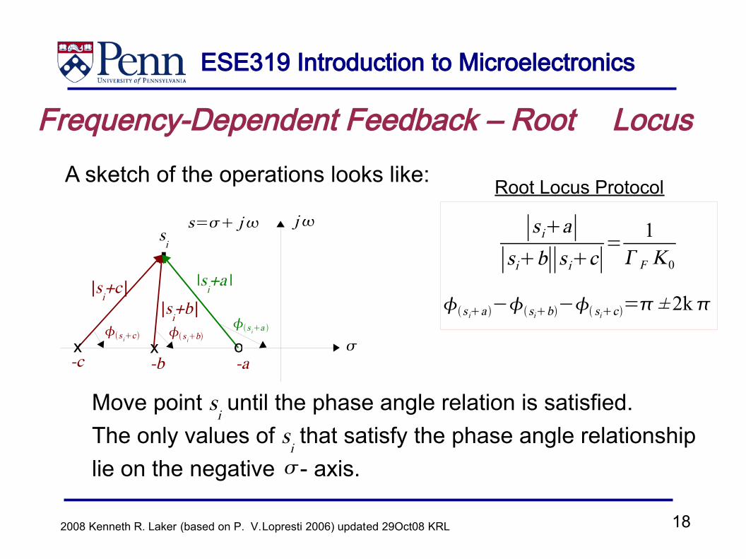
A sketch of the operations looks like:
.
-a-b-c
si
|si+c |
s ic s ibs ia
x x o
|si+b |
|si+a |
∣s ia∣∣sib∣∣s ic∣
=1
F K0
s ia −sib− sic=± 2k
Move point si until the phase angle relation is satisfied.
The only values of si that satisfy the phase angle relationship
lie on the negative - axis.
Root Locus Protocol
j
s= j
ESE319 Introduction to Microelectronics
192008 Kenneth R. Laker (based on P. V. Lopresti 2006) updated 29Oct08 KRL
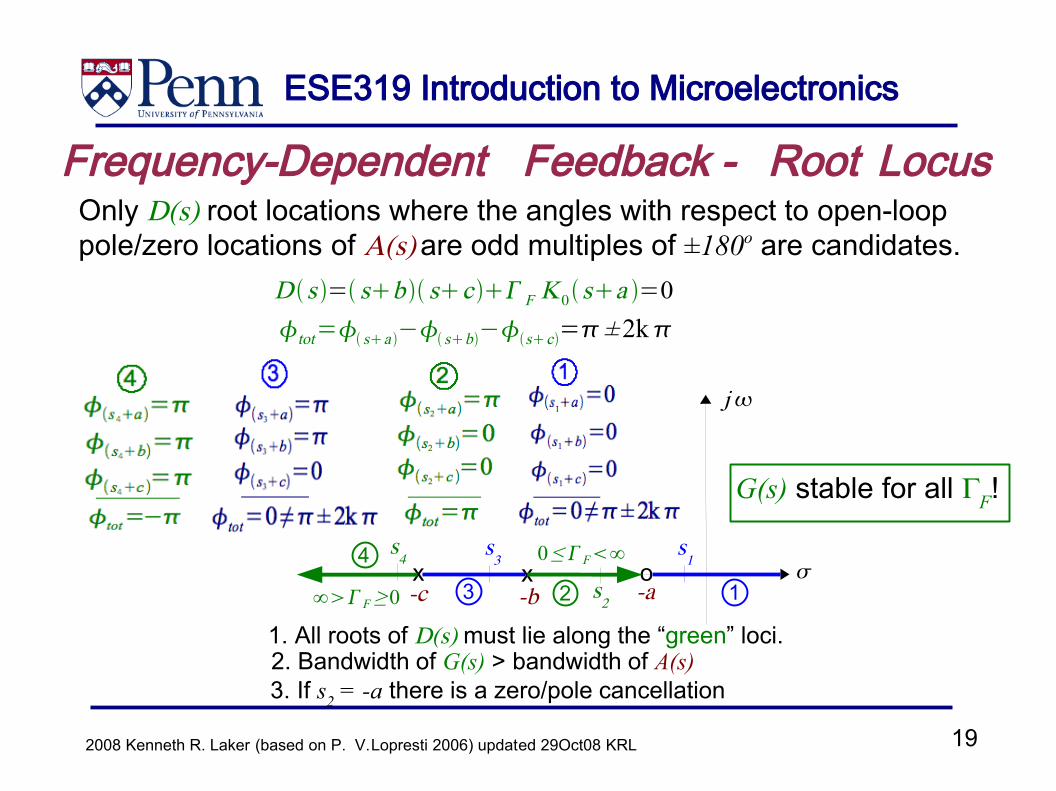
Frequency-Dependent Feedback - Root LocusOnly D(s) root locations where the angles with respect to open-loop pole/zero locations of A(s) are odd multiples of ±180o are candidates.
1. All roots of D(s) must lie along the “green” loci.
tot= sa − sb−sc=± 2kD s = sb sc F K0sa =0
∞F ≥0 -a-b-cx x o
13 2
4
j
0≤ F∞ s
1s
3s
4
s2
G(s) stable for all ΓF!
3. If s2 = -a there is a zero/pole cancellation2. Bandwidth of G(s) > bandwidth of A(s)
ESE319 Introduction to Microelectronics
202008 Kenneth R. Laker (based on P. V. Lopresti 2006) updated 29Oct08 KRL
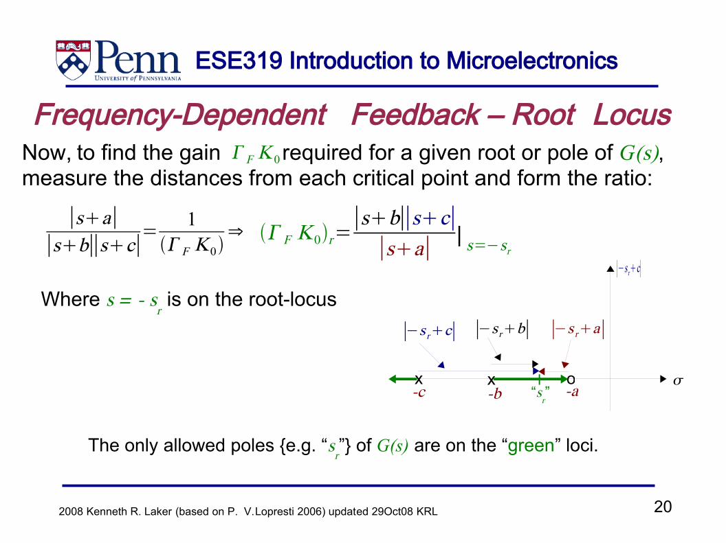
Frequency-Dependent Feedback – Root LocusNow, to find the gain required for a given root or pole of G(s), measure the distances from each critical point and form the ratio:
F K0r=∣sb∣∣sc∣
∣sa∣ s=−sr
The only allowed poles {e.g. “sr”} of G(s) are on the “green” loci.
Where s = - sr is on the root-locus
∣sa∣∣sb∣∣sc∣
= 1F K0
⇒ |∣−s rc∣
-a-b-cx x o
∣−s rb∣ ∣−s ra∣
l“s
r”
F K 0
∣−s rc∣

ESE319 Introduction to Microelectronics
212008 Kenneth R. Laker (based on P. V. Lopresti 2006) updated 29Oct08 KRL
Root Locus Two-pole A(s)
As=K0bc
sb sc
G s=K0bc
sbscF K 0bc=N sD s b c
Kω
20 log10
|A(s)| - dB
- 20 dB/dec
- 40 dB/dec
-b-cX X
∞F ≥ 0
20 log10K0
jcomplex conjugate poles of G(s)
G(s) stable for all ΓF!
Note: no zero at s = -a

ESE319 Introduction to Microelectronics
222008 Kenneth R. Laker (based on P. V. Lopresti 2006) updated 29Oct08 KRL
Root Locus Three-pole A(s)
As=K0bcd
sb scsd G s=
K 0bcdsbscsd F K 0bcd
=N sD s
-b-cX XX-d
G(s) NOT stable for all ΓF!
j
ESE319 Introduction to Microelectronics
232008 Kenneth R. Laker (based on P. V. Lopresti 2006) updated 29Oct08 KRL
The Root Locus MethodThis graphical method for finding the roots of a polynomialis known as the root locus method. It was developed beforecomputers were available. It is still used because it givesvaluable insight into the behavior of feedback systems asthe loop gain is varied. Matlab (control systems toolbox) will plot root loci.
In the frequency-dependent feedback example, we noted that increasing feedback increases the closed-loop bandwidth – i.e. the low and high frequency break points moved in opposite directions as ΓF increases. Higher ΓF , as a trade-off, reducesthe closed-loop mid-band gain.
ESE319 Introduction to Microelectronics
242008 Kenneth R. Laker (based on P. V. Lopresti 2006) updated 29Oct08 KRL
GM
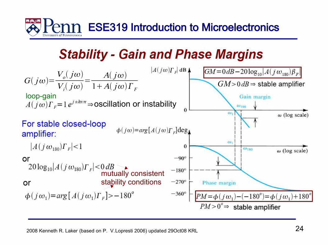
oscillation or instability
G j=Vo jV i j
=A j
1A jF
F
F
F
F
F
F
loop-gain
mutually consistent stability conditions
ESE319 Introduction to Microelectronics
252008 Kenneth R. Laker (based on P. V. Lopresti 2006) updated 29Oct08 KRL
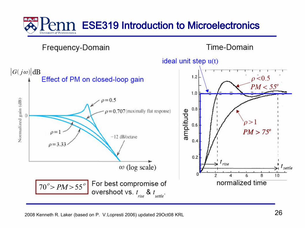
G j
∣G j∣
F
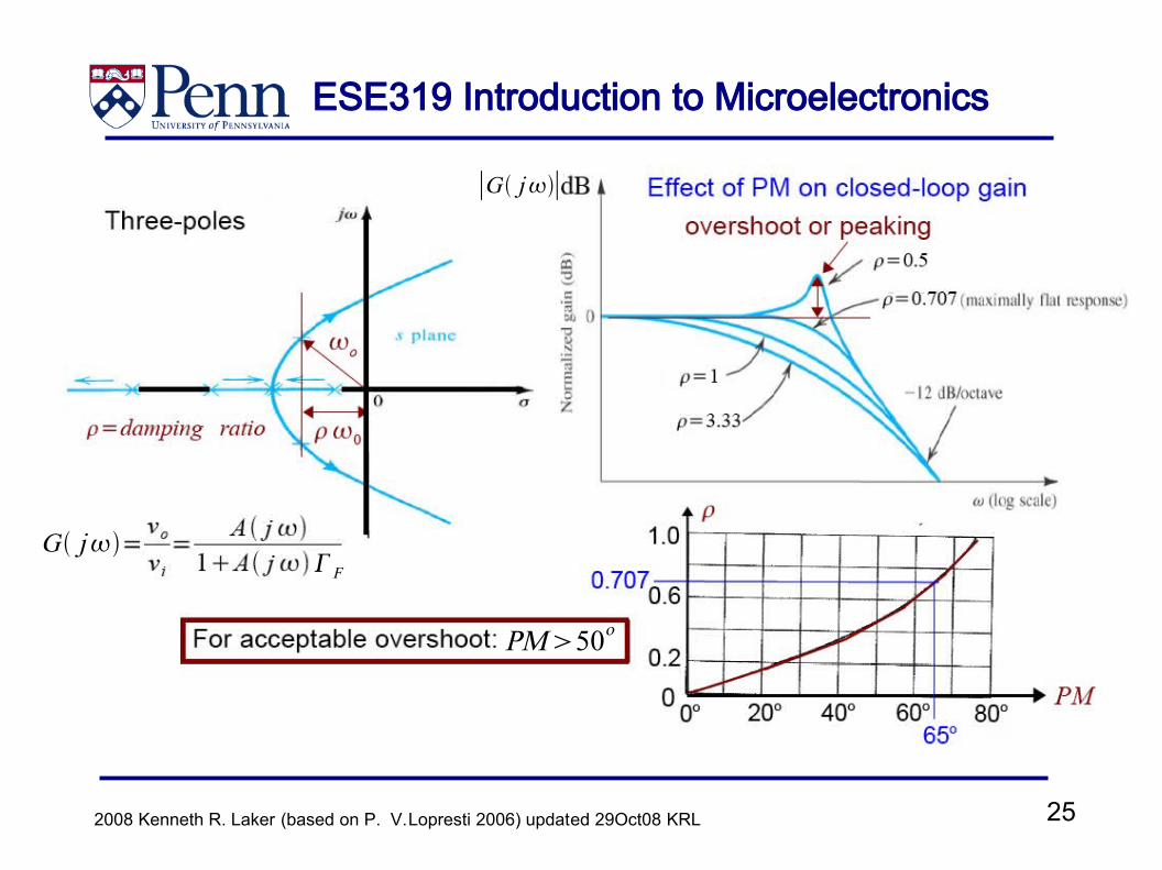
PM50o
ESE319 Introduction to Microelectronics
262008 Kenneth R. Laker (based on P. V. Lopresti 2006) updated 29Oct08 KRL
∣G j∣
70oPM55o
ESE319 Introduction to Microelectronics
272008 Kenneth R. Laker (based on P. V. Lopresti 2006) updated 29Oct08 KRL
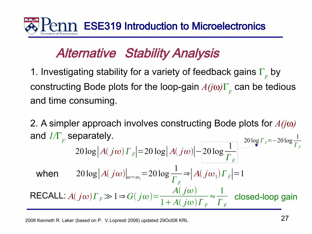
Alternative Stability Analysis1. Investigating stability for a variety of feedback gains Γ
F by
constructing Bode plots for the loop-gain A(jω)ΓF can be tedious
and time consuming.
2. A simpler approach involves constructing Bode plots for A(jω) and 1/Γ
F separately.20 log∣A jF∣=20 log∣A j∣−20 log 1
F
A jF≫1⇒G j=A j
1A jF≈1F
20 log∣A j∣=1=20 log 1
F⇒∣A j1 F∣=1
RECALL:
when
closed-loop gain
20 logF=−20 log 1F
ESE319 Introduction to Microelectronics
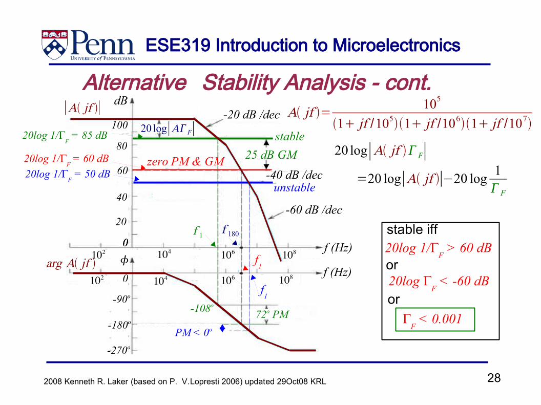
282008 Kenneth R. Laker (based on P. V. Lopresti 2006) updated 29Oct08 KRL
Alternative Stability Analysis - cont.
stable iff20log 1/Γ
F > 60 dB
or20log Γ
F < -60 dB
orΓ
F < 0.001
.=20 log∣A jf ∣−20 log 1F
-20 dB /dec
-40 dB /dec
-60 dB /dec
20 log∣AF∣20log 1/ΓF = 85 dB
20log 1/ΓF = 60 dB
20log 1/ΓF = 50 dB
dB
100
80
60
40
20
0000
-90o
-180o
-270o
-108o
72o PM
stable
zero PM & GM
unstable
f 180
25 dB GM
f 1
f1
f1
PM < 0o
∣A jf ∣
arg A jf 102 104 106 108
108106104102
A jf = 105
1 jf /1051 jf /1061 jf /107
20 log∣A jf F∣
f (Hz)
f (Hz)

ESE319 Introduction to Microelectronics
292008 Kenneth R. Laker (based on P. V. Lopresti 2006) updated 29Oct08 KRL
Alternative Stability Analysis - cont.
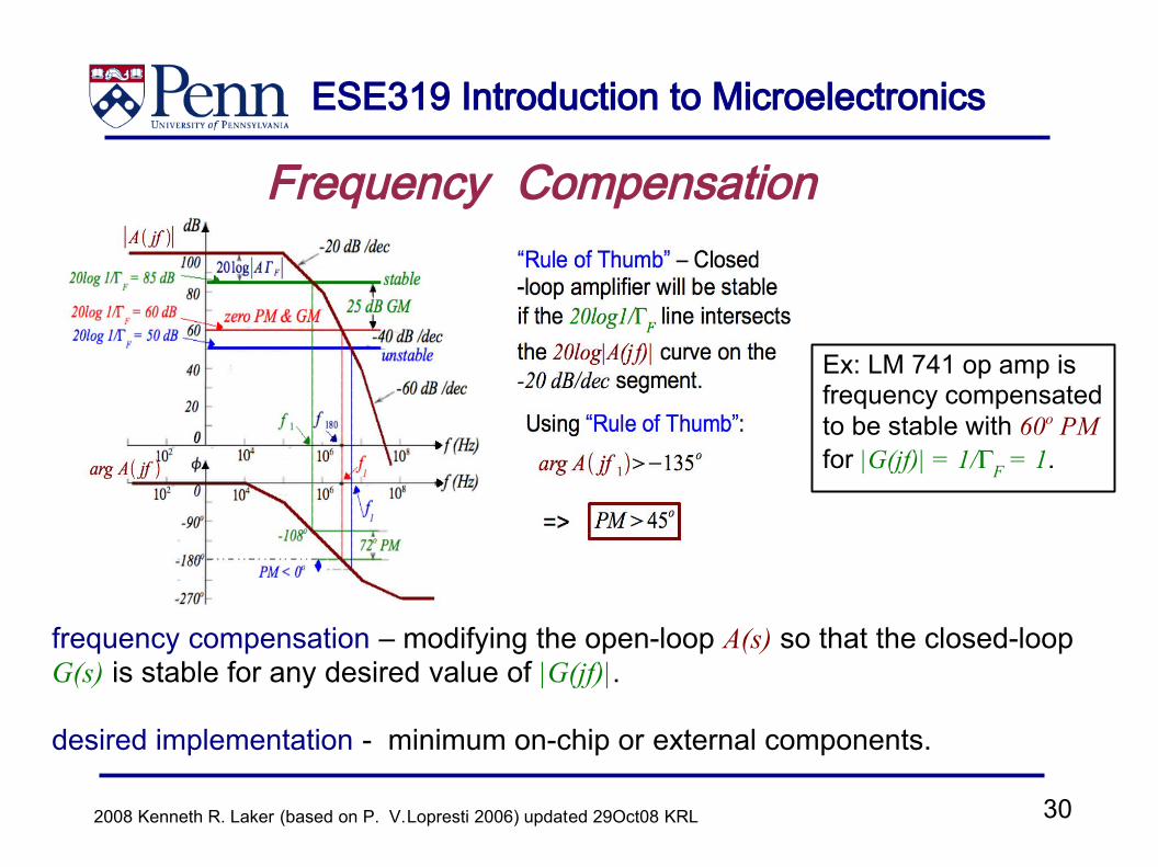
“Rule of Thumb” – Closed -loop amplifier will be stable if the 20log1/ΓF line intersects the 20log|A(j f)| curve on the -20 dB/dec segment.
Using “Rule of Thumb”:
PM45o
arg A jf 1−135o
=>
∣A jf ∣
arg A jf
ESE319 Introduction to Microelectronics
302008 Kenneth R. Laker (based on P. V. Lopresti 2006) updated 29Oct08 KRL
Frequency Compensation
frequency compensation – modifying the open-loop A(s) so that the closed-loop G(s) is stable for any desired value of |G(jf)|.
desired implementation - minimum on-chip or external components.
Ex: LM 741 op amp is frequency compensated to be stable with 60o PM for |G(jf)| = 1/ΓF = 1.
ESE319 Introduction to Microelectronics
312008 Kenneth R. Laker (based on P. V. Lopresti 2006) updated 29Oct08 KRL
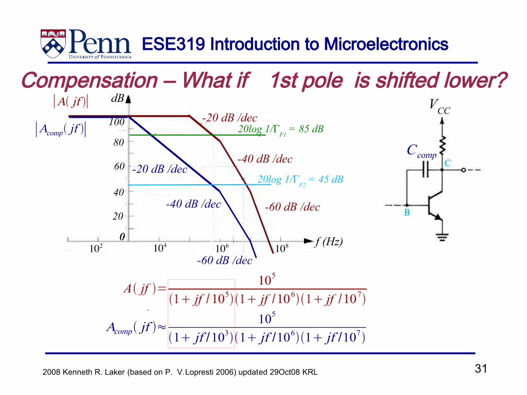
Compensation – What if 1st pole is shifted lower?VCC
dB
100
80
60
40
20
0000
-90o
-180o
-270o
∣A jf ∣
102 104 106 108
108106104
-20 dB /dec
-40 dB /dec
-60 dB /dec
-60 dB /dec
-40 dB /dec
-20 dB /dec
∣Acomp jf ∣ 20log 1/ΓF1
= 85 dB
20log 1/ΓF2
= 45 dB
Acomp jf ≈105
1 jf /1031 jf /1061 jf /107
f (Hz)
C comp
ESE319 Introduction to Microelectronics
322008 Kenneth R. Laker (based on P. V. Lopresti 2006) updated 29Oct08 KRL
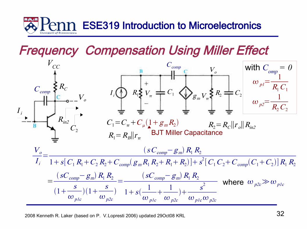
Frequency Compensation Using Miller EffectVCC Ccomp
C1 C2R1 R2V gmVI i
I i
Vo
Vo
C1=CC 1gmR2R1=RB∥r
RC
R2=RC∥r o∥Rin2Rin2
C2
Vo
I i=
sC comp−gmR1R21s [C1R1C2R2C compgmR1R2R1R2]s
2[C1C 2C compC 1C2]R1R2
.=sC comp−gmR1R2
1 sp1c
1 sp2c
=
sC comp−gmR1R2
1s 1 p1c
1 p2c
s2
p1cp2c
where p2c≫p1c
p1=1R1C1
p2=1R2C2
BJT Miller Capacitance
with Comp = 0
C comp
ESE319 Introduction to Microelectronics
332008 Kenneth R. Laker (based on P. V. Lopresti 2006) updated 29Oct08 KRL
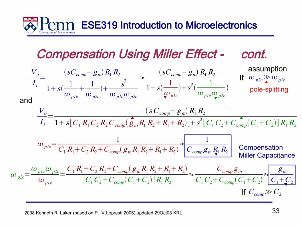
Compensation Using Miller Effect - cont.Vo
I i=
sC comp−gmR1R2
1s 1 p1c
1 p2c
s2
p1cp2c
≈sC comp−gmR1R2
1s 1p1c
s2 1p1c p2c
p2c≫p1cIf
Vo
I i=
sC comp−gmR1R21s [C1R1C 2R2C compgmR1R2R1R2]s
2[C1C2C compC1C 2]R1R2
and
p1c=1
C1R1C2R2C compgmR1R2R1R2≈ 1C compgmR1R2
p2c= p1c p2c
p1c=C1R1C2R2C compgmR1R2R1R2
[C1C2C compC1C 2]R1R2≈
C comp gmC1C2C compC1C 2
≈gm
C1C 2
C comp≫C 2
pole-splitting
assumption
Compensation Miller Capacitance
If
ESE319 Introduction to Microelectronics
342008 Kenneth R. Laker (based on P. V. Lopresti 2006) updated 29Oct08 KRL
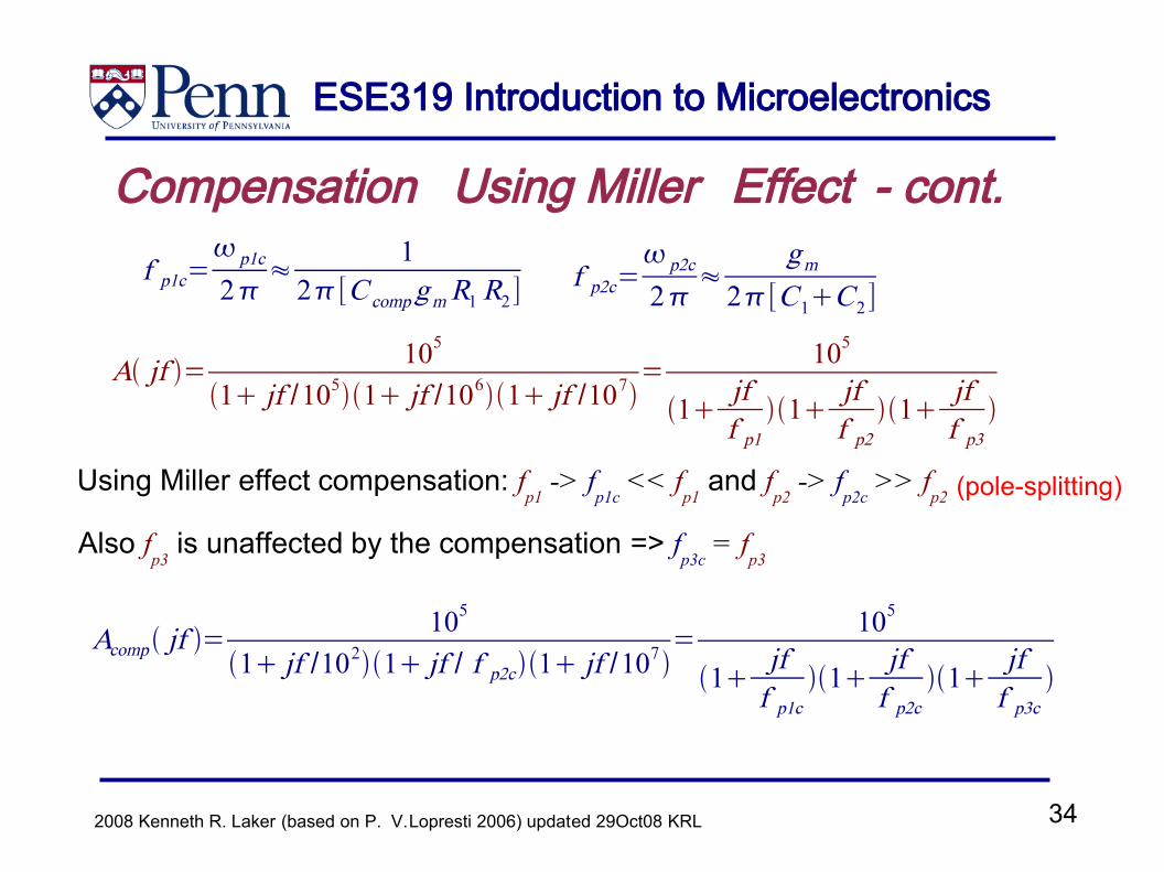
Compensation Using Miller Effect - cont.f p1c=
p1c
2≈
12 [C compgmR1R2]
f p2c= p2c
2≈
gm2 [C1C2]
A jf = 105
1 jf /1051 jf /1061 jf /107= 105
1 jff p1
1 jff p2
1 jff p3
Using Miller effect compensation: fp1
-> fp1c
<< fp1
and fp2
-> fp2c
>> fp2
Also fp3
is unaffected by the compensation => fp3c
= fp3
Acomp jf =105
1 jf /1021 jf / f p2c1 jf /107= 105
1 jff p1c
1 jff p2c
1 jff p3c
(pole-splitting)
ESE319 Introduction to Microelectronics
352008 Kenneth R. Laker (based on P. V. Lopresti 2006) updated 29Oct08 KRL
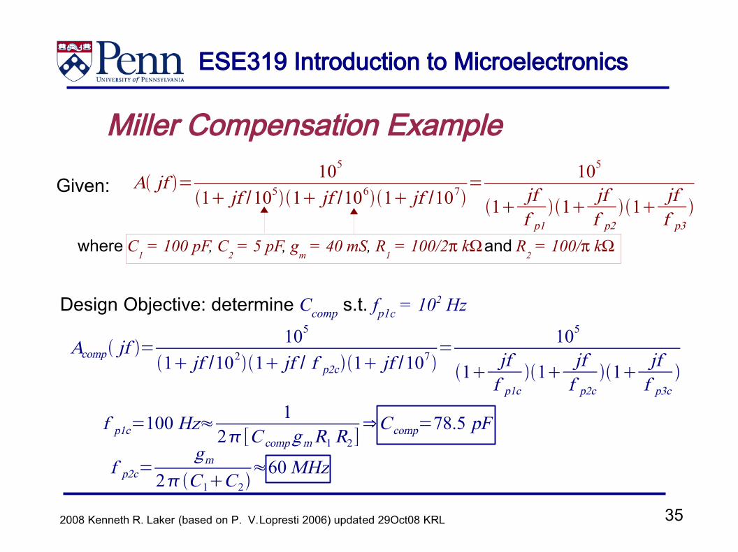
Miller Compensation Example
Design Objective: determine Ccomp s.t. fp1c = 102 Hz
Given: A jf = 105
1 jf /1051 jf /1061 jf /107= 105
1 jff p1
1 jff p2
1 jff p3
f p2c=gm
2C1C2≈60MHz
Acomp jf =105
1 jf /1021 jf / f p2c1 jf /107= 105
1 jff p1c
1 jff p2c
1 jff p3c
where C1 = 100 pF, C
2 = 5 pF, g
m = 40 mS, R
1 = 100/2π kΩ and R
2 = 100/π kΩ
f p1c=100 Hz≈1
2 [C compgmR1R2]⇒C comp=78.5 pF
ESE319 Introduction to Microelectronics
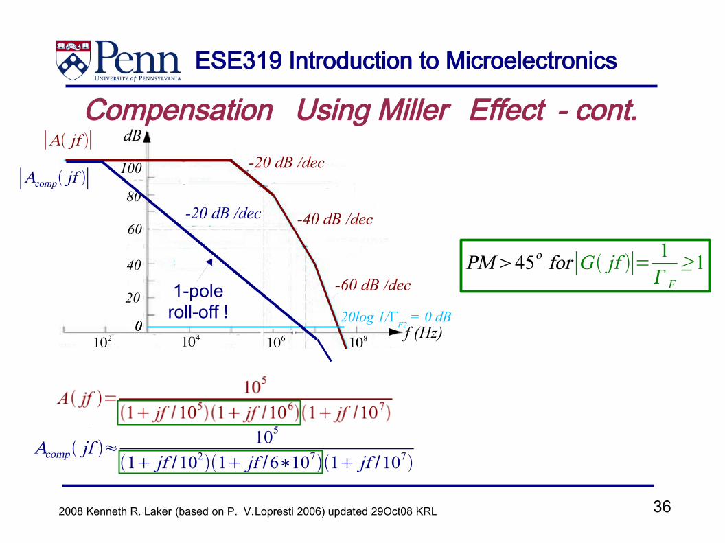
362008 Kenneth R. Laker (based on P. V. Lopresti 2006) updated 29Oct08 KRL
Compensation Using Miller Effect - cont.dB
100
80
60
40
20
000
∣A jf ∣
102 104 106 108
-20 dB /dec
-40 dB /dec
-60 dB /dec
-60 dB /dec -40 dB /dec
-20 dB /dec
∣Acomp jf ∣
20log 1/ΓF2
= 0 dBf (Hz)
0
-90o
-180o
-270o
108106104
1-pole roll-off !
Acomp jf ≈105
1 jf /1021 jf /6∗1071 jf /107
PM45o for∣G jf ∣= 1F≥1

ESE319 Introduction to Microelectronics
372008 Kenneth R. Laker (based on P. V. Lopresti 2006) updated 29Oct08 KRL
SummaryFeedback has many desirable features, but it can createunexpected - undesired results if the full frequency-dependent nature (phase-shift with frequency) of the feedback circuit is not taken into account.
We next will use feedback to convert a well-behaved stablecircuit into an oscillator. Sometimes, because of parasitics,feedback in amplifiers turns them into unexpected oscillators.
The root-locus method was used to help us understand how feedback can create the conditions for oscillation and instability.
Related Documents


