1 FEC 512 Financial Econometrics -About the Course- • What is Financial Econometrics? – Science of modeling and forecasting financial time series. • Who is this course for? – Students in finance, practitioners in the financial services sector. • How is the presentation of the lectures? – Begins with review of necessary statistics and probability theory, continues with basics of econometrics reaches up to the most recent theoretical results – Uses computer applications, Eviews. – Course materials are online at online.bilgi.edu.tr – Students are supposed to choose a data set from the list at the beginning of the term in order to do assignments – Attendence is not required.

Welcome message from author
This document is posted to help you gain knowledge. Please leave a comment to let me know what you think about it! Share it to your friends and learn new things together.
Transcript
1
FEC 512 Financial Econometrics-About the Course-
• What is Financial Econometrics?
– Science of modeling and forecasting financial time series.
• Who is this course for?
– Students in finance, practitioners in the financial services sector.
• How is the presentation of the lectures?
– Begins with review of necessary statistics and probability theory, continues with basics of econometrics reaches up to the most recent theoretical results
– Uses computer applications, Eviews.
– Course materials are online at online.bilgi.edu.tr
– Students are supposed to choose a data set from the list at the beginning of the term in order to do assignments
– Attendence is not required.
2
FEC 512 Financial Econometrics-About the Course-
• Textbooks:
1. (for Statistics part only) Groebner D.F. et al.(2008) Business Statistics.
2. Ruppert D. (2004), Statistics and Finance, Springer.
3. Brooks, C. “Introductory Econometics for Finance”
4. Stock J.H. and Watson M.W. (2003), Introduction to Econometrics (first edition), Addison-Wesley.
• Method of Evaluation:– Assignments (50%)
– Final Examination (50% )
3
Overview
Before getting into applications in financialeconometrics we will first define
• returns on assets
Then we will review• Probability
– probability density functions, cumulative distribution functions
– expectations, variance, covariance and correlation
• Statistics– Testing
– Estimation
• We’ll also be studying some new areas of statistics:– Regression
• interesting connections with portfolio analysis.
– Probit, Logit Analysis
– Time series models
FEC 512 Preliminaries and Review Lecture 1-4
I. Preliminary: Asset Return
Calculations
Istanbul Bilgi University
FEC 512 Financial Econometrics-I
Asst. Prof. Dr. Orhan Erdem
FEC 512 Preliminaries and Review Lecture 1-5
Background
� How do the prices of stocks and other
financial assets behave?
� We will start by defining returns on the prices
of a stock.
FEC 512 Preliminaries and Review Lecture 1-6
Prices and Returns
� Main data of financial econometrics are asset
prices and returns.
� Almost all empirical research analyzes
returns to investors rather than prices. Why?
� Investors are interested in revenues that are
high r.t. size of the initial invstmnt. Returns
measure this: Changes in prices expressed
as a fraction of the initial price.
FEC 512 Preliminaries and Review Lecture 1-7
Asset Return Calculations
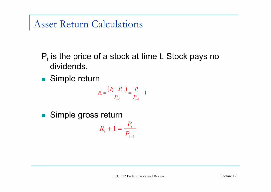
Pt is the price of a stock at time t. Stock pays no
dividends.
� Simple return
� Simple gross return
1
1 tt
t
PR
P −
+ =
( )11 1
1t t t
t
t t
P P PR
P P
−
− −
−= = −
FEC 512 Preliminaries and Review Lecture 1-8
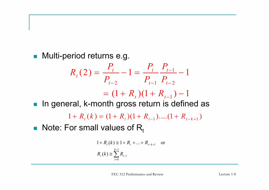
� Multi-period returns e.g.
� In general, k-month gross return is defined as
� Note: For small values of Rt
1
2 1 2
1
(2) 1 1
(1 )(1 ) 1
t t tt
t t t
t t
P P PR
P P P
R R
−
− − −
−
= − = −
= + + −
1 11 ( ) (1 )(1 )....(1 )t t t t kR k R R R− − ++ = + + +
∑−
=−
+−
≅
+++≅+1
0
1
)(
or ...1)(1
k
i
itt
kttt
RkR
RRkR
FEC 512 Preliminaries and Review Lecture 1-9
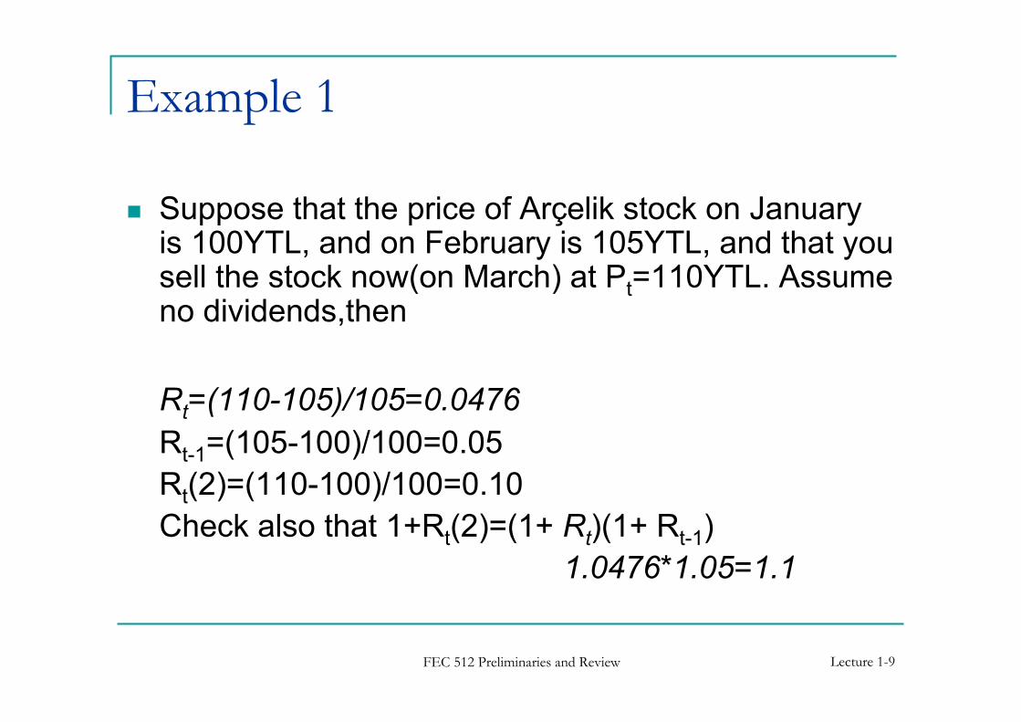
Example 1
� Suppose that the price of Arçelik stock on January is 100YTL, and on February is 105YTL, and that yousell the stock now(on March) at Pt=110YTL. Assumeno dividends,then
Rt=(110-105)/105=0.0476
Rt-1=(105-100)/100=0.05
Rt(2)=(110-100)/100=0.10
Check also that 1+Rt(2)=(1+ Rt)(1+ Rt-1)
1.0476*1.05=1.1
FEC 512 Preliminaries and Review Lecture 1-10
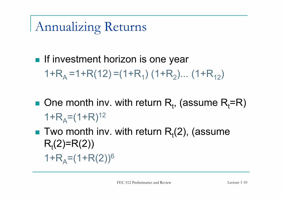
Annualizing Returns
� If investment horizon is one year
1+RA =1+R(12) =(1+R1) (1+R2)... (1+R12)
� One month inv. with return Rt, (assume Rt=R)
1+RA=(1+R)12
� Two month inv. with return Rt(2), (assume
Rt(2)=R(2))
1+RA=(1+R(2))6
FEC 512 Preliminaries and Review Lecture 1-11
Cont. to Example 1
� In the first example the one month return was
4.76%. If we assume that we can get this
return for 12 months then the annualized
return is
RA=(1.0476)12-1=1.7472-1=0.7472 or 74.72%
FEC 512 Preliminaries and Review Lecture 1-12
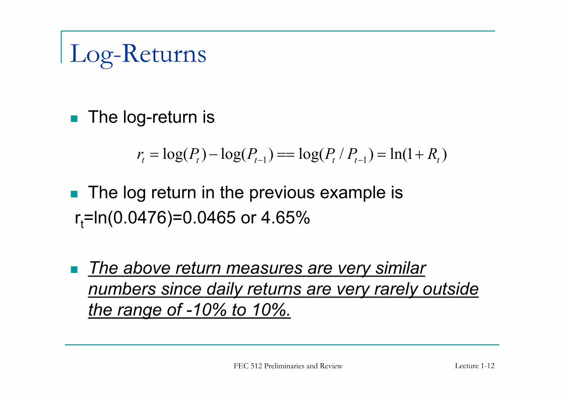
Log-Returns
� The log-return is
� The log return in the previous example is
rt=ln(0.0476)=0.0465 or 4.65%
� The above return measures are very similar
numbers since daily returns are very rarely outside
the range of -10% to 10%.
)1ln()/log()log()log( 11 tttttt RPPPPr +===−= −−
FEC 512 Preliminaries and Review Lecture 1-13
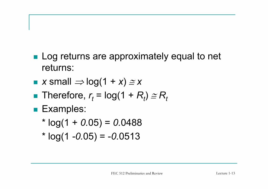
� Log returns are approximately equal to net
returns:
� x small ⇒ log(1 + x) ≅ x
� Therefore, rt = log(1 + Rt) ≅ Rt
� Examples:
* log(1 + 0.05) = 0.0488
* log(1 -0.05) = -0.0513
FEC 512 Preliminaries and Review Lecture 1-14
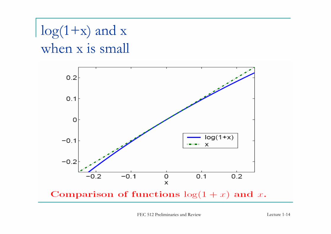
log(1+x) and x
when x is small
FEC 512 Preliminaries and Review Lecture 1-15
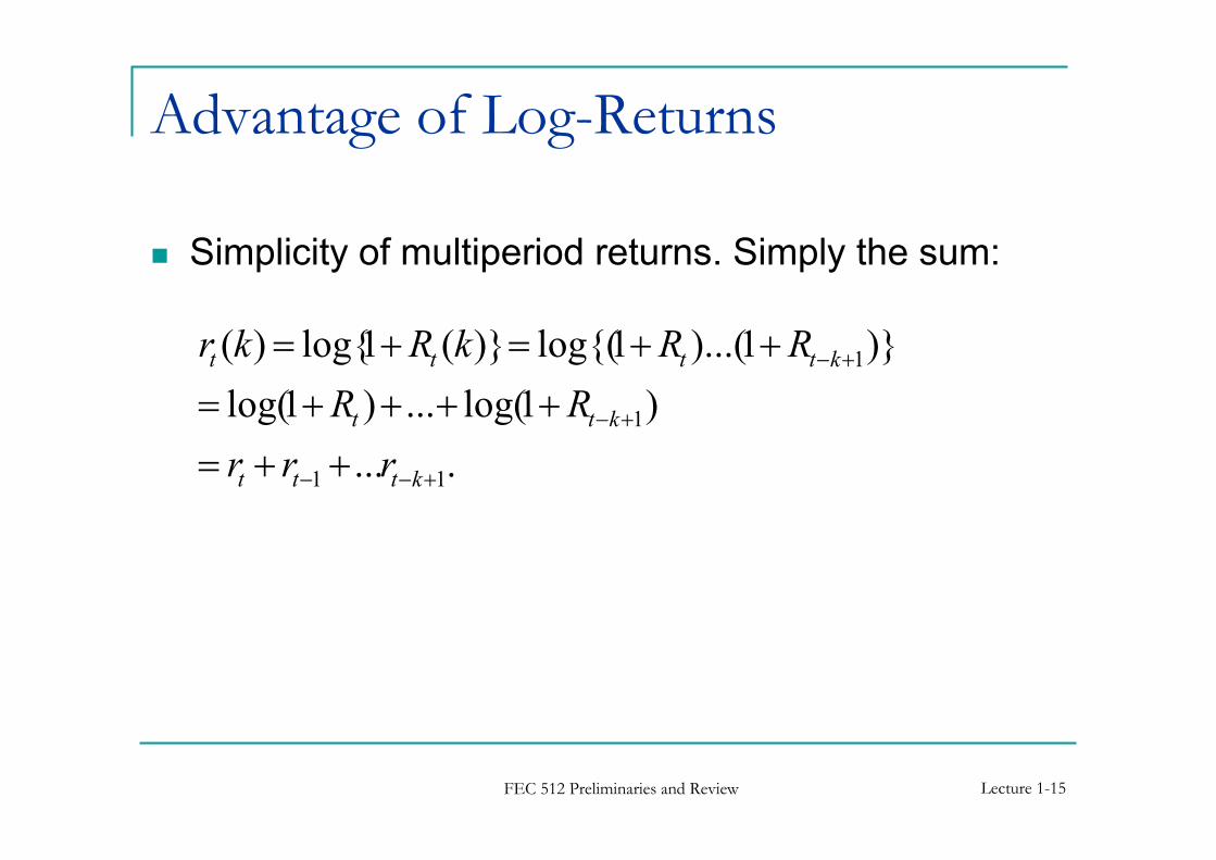
Advantage of Log-Returns
� Simplicity of multiperiod returns. Simply the sum:
....
)1log(...)1log(
)}1)...(1log{()}(1log{)(
11
1
1
+−−
+−
+−
++=
++++=
++=+=
kttt
ktt
ktttt
rrr
RR
RRkRkr
FEC 512 Preliminaries and Review Lecture 1-16
Returns are
� scale-free, meaning that they do not depend
on monetary units (dollars, cents, etc.)
� not unit-less, unit is time; they depend on the
units of t (hour, day, etc.)
FEC 512 Preliminaries and Review Lecture 1-17
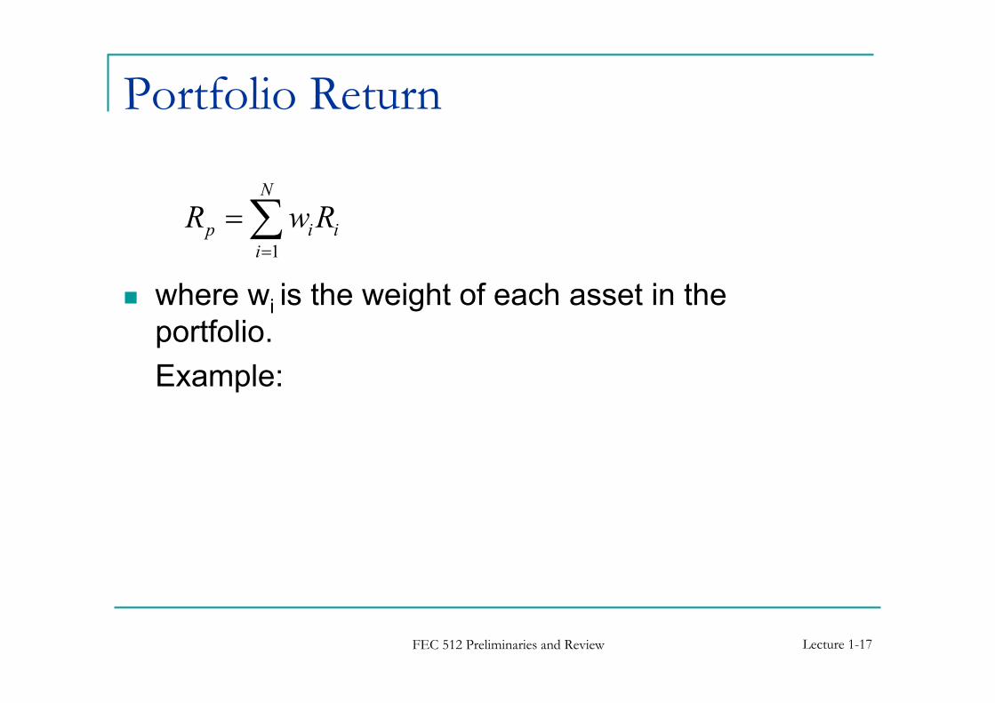
Portfolio Return
� where wi is the weight of each asset in the
portfolio.
Example:
1
N
p i i
i
R w R=
=∑
FEC 512 Preliminaries and Review Lecture 1-18
About Returns
� Returns cannot be perfectly predicted, they
are random.
� This randomness implies that a return might
be smaller than its expected value and even
negative, which means that investing involves
RISK.
� It took quite some time before it was realized
that risk could be described by probability
theory
FEC 512 Preliminaries and Review Lecture 1-19
II. Review of Probability &
Statistics
FEC 512 Preliminaries and Review Lecture 1-20
Probability and Finance
� Because we cannot build purelydeterministic models of the economy, weneed a mathematical representation of uncertainty in finance (probability, fuzzymeasures etc…)
� In economic and finance theory, probabilitymight have 2 meanings:
1. As a descriptive concept
2. As a determinant of the agent decisionmaking theory.
FEC 512 Preliminaries and Review Lecture 1-21
Probability as a Descriptive Concept
� The probability of an event is assumed to be
approx. equal to the rel.freq. of its occurrence
in a large # experiments.
� There is one difficulty with this interpretation:
� Empirical data have only one realization.
� Every estimate is made on a single time-evolving
series.
� If stationarity(!) is not assumed, performing
statistical estimation is impossible.
FEC 512 Preliminaries and Review Lecture 1-22
Probability Concepts
� Experiment – a process of obtaining
outcomes for uncertain events
� Outcome – the possible results of an
observation, such as the price of a security
at t.
� However, probability statements are not
made on outcomes but on events, which are
sets of possible outcomes.
� The Sample Space is the collection of all
possible outcomes
FEC 512 Preliminaries and Review Lecture 1-23
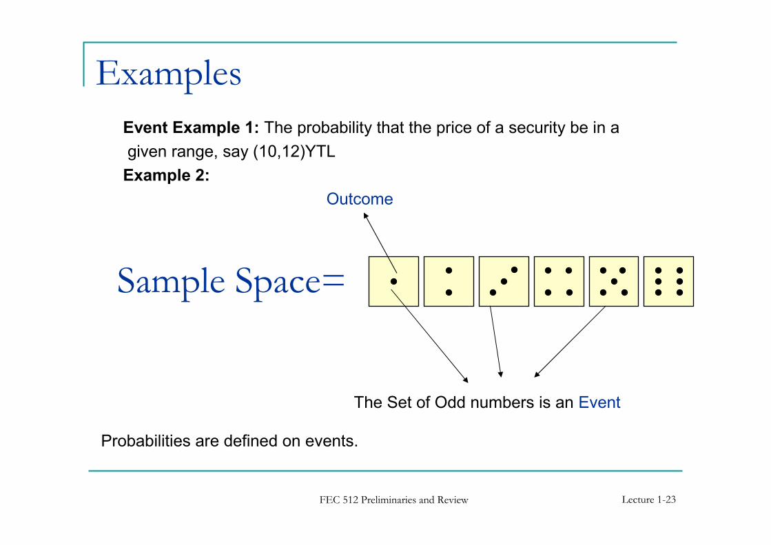
Sample Space=
Outcome
The Set of Odd numbers is an Event
Event Example 1: The probability that the price of a security be in a
given range, say (10,12)YTL
Example 2:
Probabilities are defined on events.
Examples
FEC 512 Preliminaries and Review Lecture 1-24
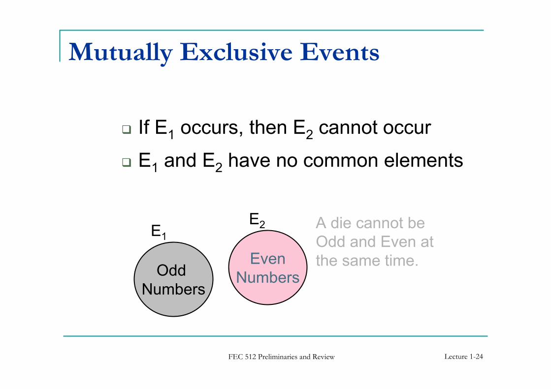
Mutually Exclusive Events
� If E1 occurs, then E2 cannot occur
� E1 and E2 have no common elements
Odd
Numbers
Even
Numbers
A die cannot be
Odd and Even at
the same time.
E1
E2
FEC 512 Preliminaries and Review Lecture 1-25
� Independent: Occurrence of one does not
influence the probability of occurrence of
the other
� Dependent: Occurrence of one affects the
probability of the other
Independent and Dependent
Events
FEC 512 Preliminaries and Review Lecture 1-26
Independent vs. Dependent Events
� Independent Events
E1 = heads on one flip of fair coin
E2 = heads on second flip of same coin
Result of second flip does not depend on the
result of the first flip.
� Dependent Events
E1 = rain forecasted on the news
E2 = take umbrella to work
Probability of the second event is affected by the
occurrence of the first event
FEC 512 Preliminaries and Review Lecture 1-27
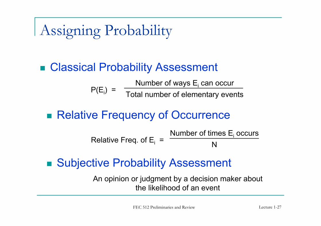
Assigning Probability
� Classical Probability Assessment
� Relative Frequency of Occurrence
� Subjective Probability Assessment
P(Ei) =Number of ways Ei can occur
Total number of elementary events
Relative Freq. of Ei =Number of times Ei occurs
N
An opinion or judgment by a decision maker about
the likelihood of an event
FEC 512 Preliminaries and Review Lecture 1-28
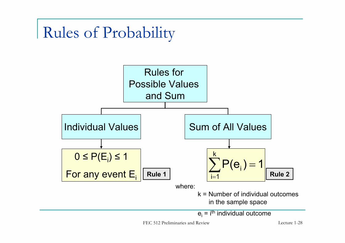
Rules of Probability
Rules for
Possible Values
and Sum
Individual Values Sum of All Values
0 ≤ P(Ei) ≤ 1
For any event Ei
1)P(ek
1i
i =∑=
where:
k = Number of individual outcomes
in the sample space
ei = ith individual outcome
Rule 1 Rule 2
FEC 512 Preliminaries and Review Lecture 1-29
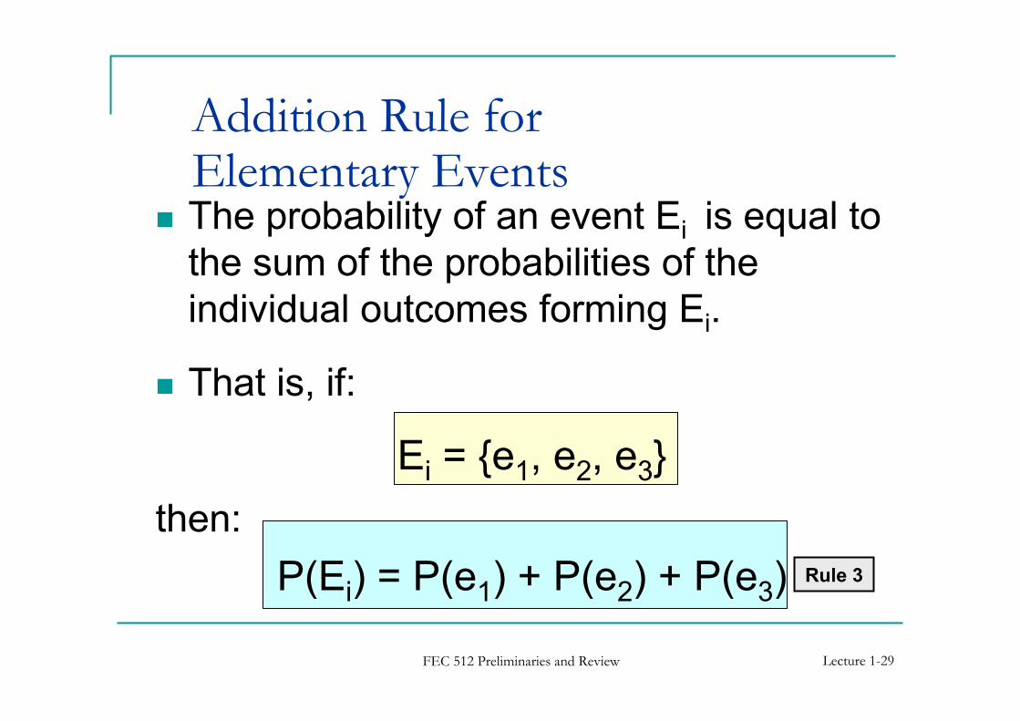
Addition Rule forElementary Events
Rule 3
� The probability of an event Ei is equal to
the sum of the probabilities of the
individual outcomes forming Ei.
� That is, if:
Ei = {e1, e2, e3}
then:
P(Ei) = P(e1) + P(e2) + P(e3)
FEC 512 Preliminaries and Review Lecture 1-30
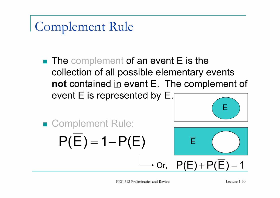
Complement Rule
� The complement of an event E is the
collection of all possible elementary events
not contained in event E. The complement of
event E is represented by E.
� Complement Rule:
P(E)1)EP( −= E
E
1)EP(P(E) =+Or,
FEC 512 Preliminaries and Review Lecture 1-31
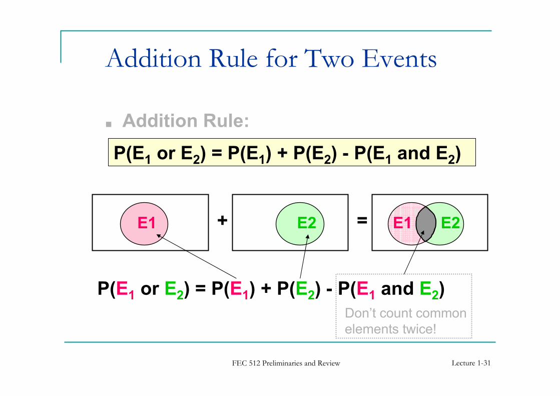
Addition Rule for Two Events
P(E1 or E2) = P(E1) + P(E2) - P(E1 and E2)
E1 E2
P(E1 or E2) = P(E1) + P(E2) - P(E1 and E2)
Don’t count common
elements twice!
■ Addition Rule:
E1 E2+ =
FEC 512 Preliminaries and Review Lecture 1-32
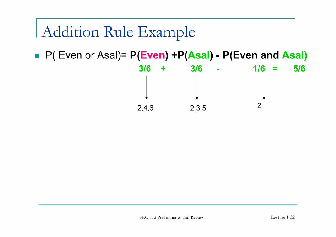
Addition Rule Example
� P( Even or Asal)= P(Even) +P(Asal) - P(Even and Asal)
3/6 + 3/6 - 1/6 = 5/6
2,4,6 2,3,5 2

FEC 512 Preliminaries and Review Lecture 1-33
Addition Rule for Mutually Exclusive Events
� If E1 and E2 are mutually exclusive, then
P(E1 and E2) = 0
So
P(E1 or E2) = P(E1) + P(E2) - P(E1 and E2)
= P(E1) + P(E2)
= 0
E1 E2
if mutu
ally
exclusiv
e
FEC 512 Preliminaries and Review Lecture 1-34
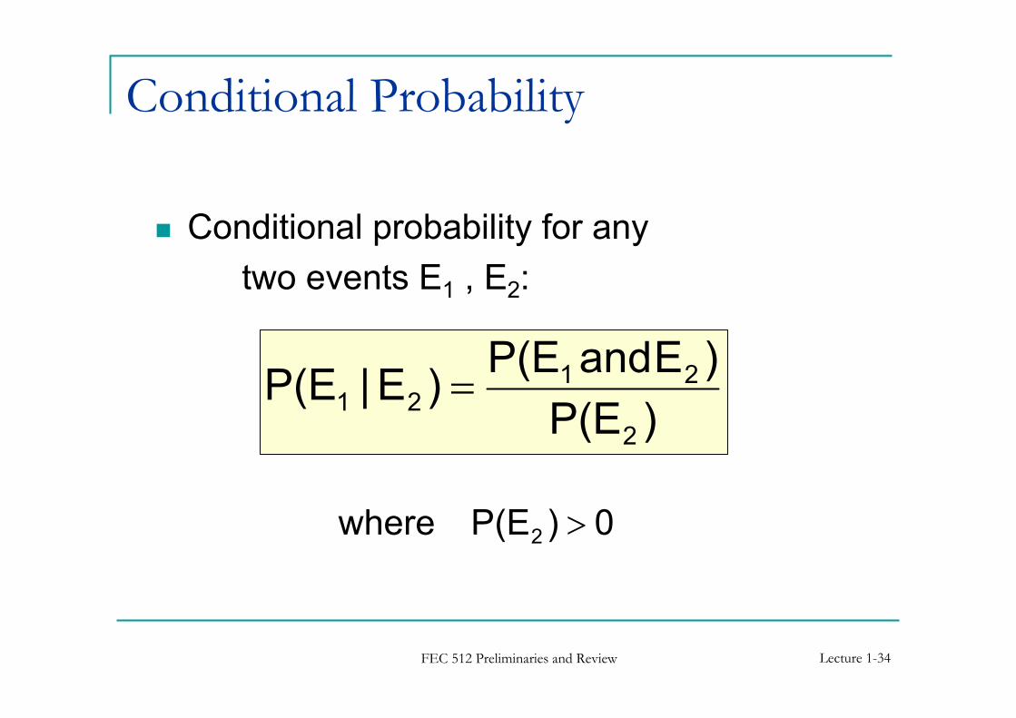
Conditional Probability
� Conditional probability for any
two events E1 , E2:
)P(E
)EandP(E)E|P(E
2
2121 =
0)P(Ewhere 2 >
FEC 512 Preliminaries and Review Lecture 1-35
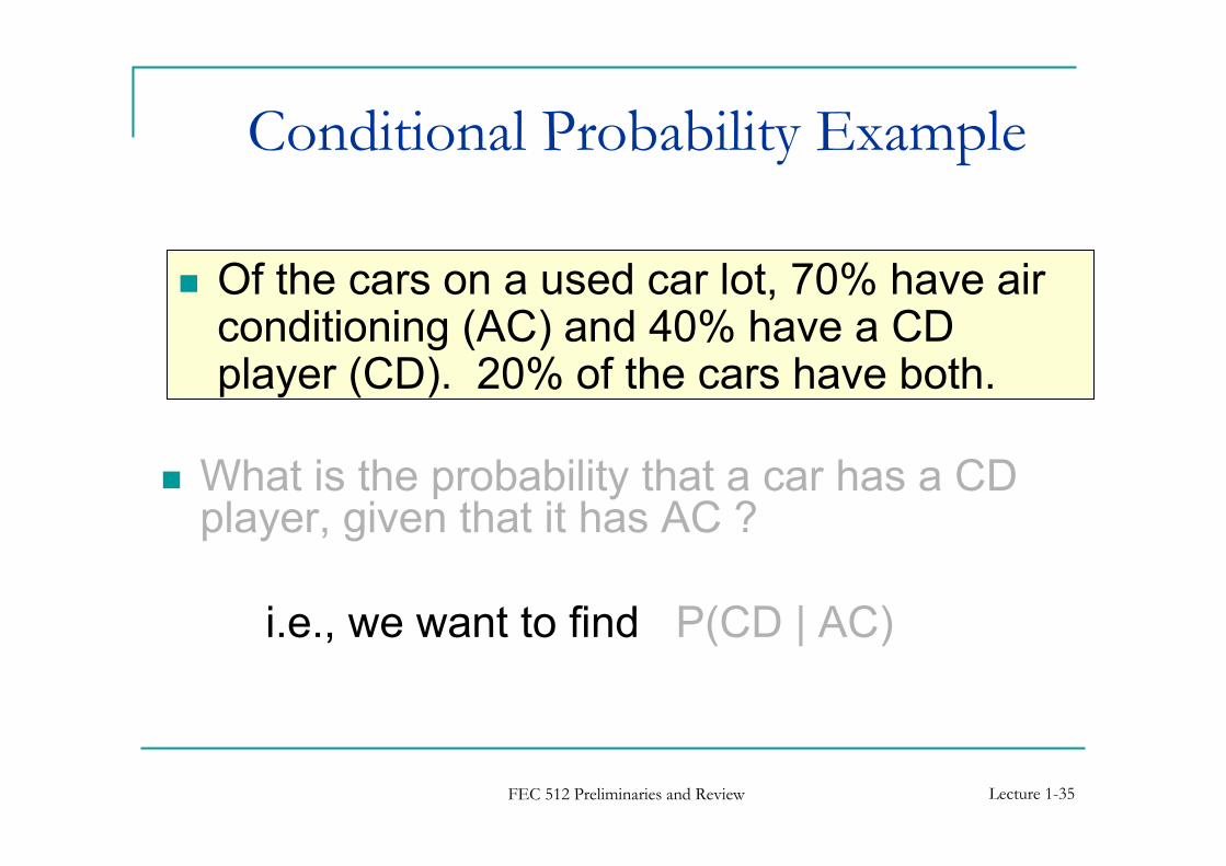
� What is the probability that a car has a CD player, given that it has AC ?
i.e., we want to find P(CD | AC)
Conditional Probability Example
� Of the cars on a used car lot, 70% have air conditioning (AC) and 40% have a CD player (CD). 20% of the cars have both.
FEC 512 Preliminaries and Review Lecture 1-36
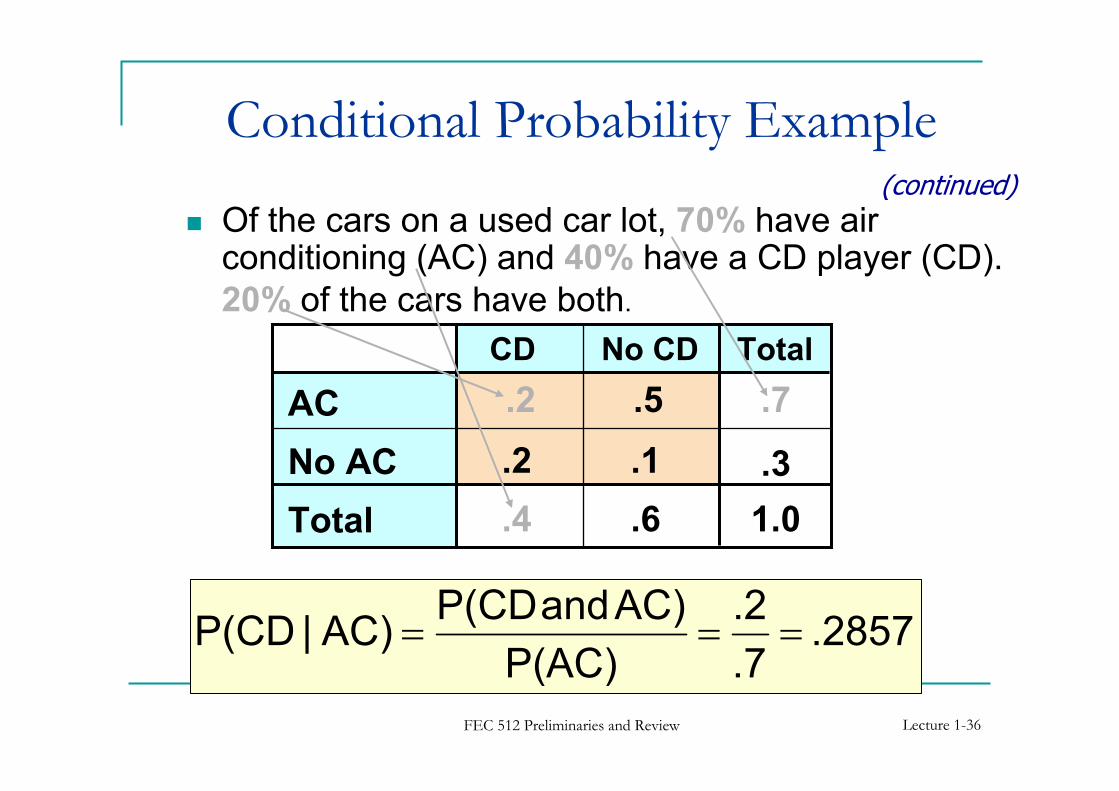
Conditional Probability Example
No CDCD Total
AC .2 .5 .7
No AC .2 .1 .3
Total .4 .6 1.0
� Of the cars on a used car lot, 70% have air conditioning (AC) and 40% have a CD player (CD).
20% of the cars have both.
.2857.7
.2
P(AC)
AC)andP(CDAC)|P(CD ===
(continued)
FEC 512 Preliminaries and Review Lecture 1-37
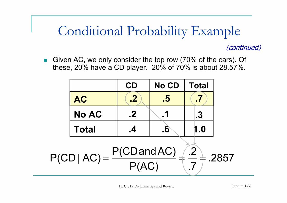
Conditional Probability Example
No CDCD Total
AC .2 .5 .7
No AC .2 .1 .3
Total .4 .6 1.0
� Given AC, we only consider the top row (70% of the cars). Of these, 20% have a CD player. 20% of 70% is about 28.57%.
.2857.7
.2
P(AC)
AC)andP(CDAC)|P(CD ===
(continued)
FEC 512 Preliminaries and Review Lecture 1-38
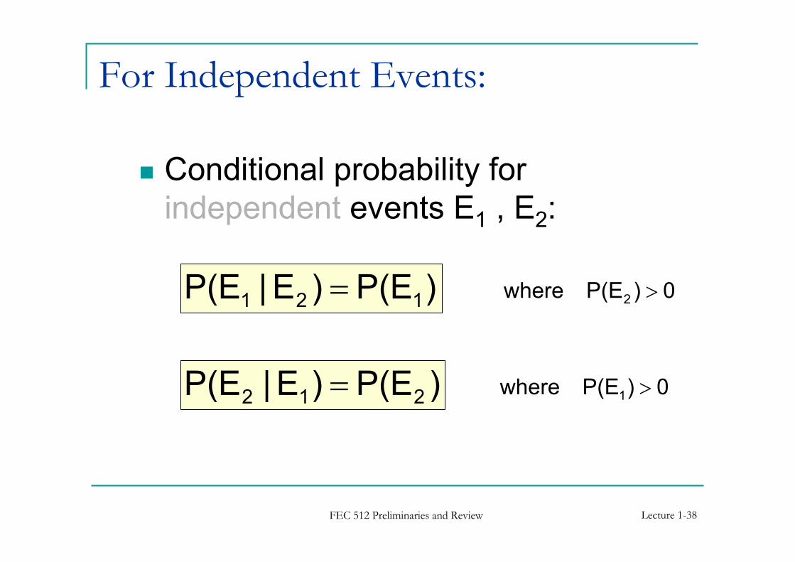
For Independent Events:
� Conditional probability for
independent events E1 , E2:
)P(E)E|P(E 121 = 0)P(Ewhere 2 >
)P(E)E|P(E 212 = 0)P(Ewhere 1 >
FEC 512 Preliminaries and Review Lecture 1-39
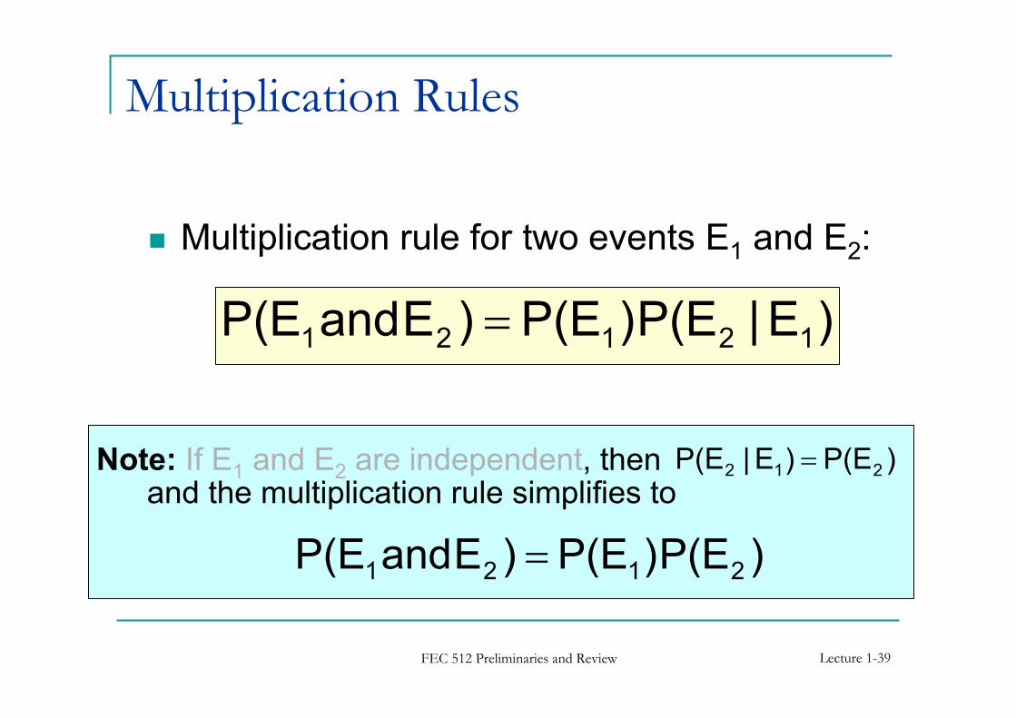
Multiplication Rules
� Multiplication rule for two events E1 and E2:
)E|P(E)P(E)EandP(E 12121 =
)P(E)E|P(E 212 =Note: If E1 and E2 are independent, thenand the multiplication rule simplifies to
)P(E)P(E)EandP(E 2121 =
FEC 512 Preliminaries and Review Lecture 1-40
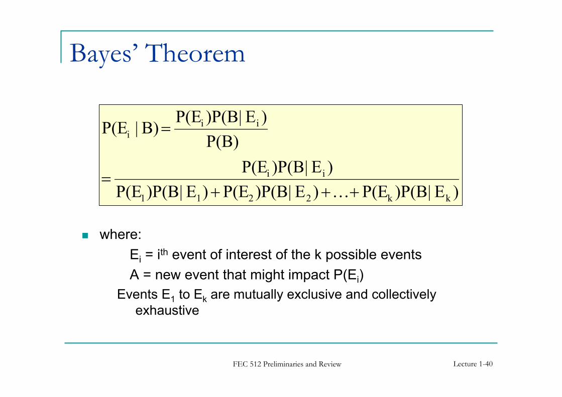
Bayes’ Theorem
� where:
Ei = ith event of interest of the k possible events
A = new event that might impact P(Ei)
Events E1 to Ek are mutually exclusive and collectively
exhaustive
)E|)P(BP(E)E|)P(BP(E)E|)P(BP(E
)E|)P(BP(E
P(B)
)E|)P(BP(EB)|P(E
kk2211
ii
iii
+++=
=
K
FEC 512 Preliminaries and Review Lecture 1-41
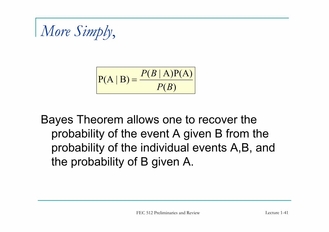
More Simply,
Bayes Theorem allows one to recover the
probability of the event A given B from the
probability of the individual events A,B, and
the probability of B given A.
)(
P(A))A|(B)|P(A
BP
BP=

FEC 512 Preliminaries and Review Lecture 1-42
Bayes’ Theorem Example
Suppose that the probability that the price of a
stock will rise on any given day, is 0.5. Thus,
we have the prior probabilities
P(Rise)=0.5 and P(No rise)=0.5.
When it actually rises, the brokers correctly
forecasts the rise 30% of the time. When it
does not rise, they incorrectly forecast rise 6%
of the time. What is the probability that the
prices will rise if the brokers forecasted that it
will rise tomorrow?
FEC 512 Preliminaries and Review Lecture 1-43
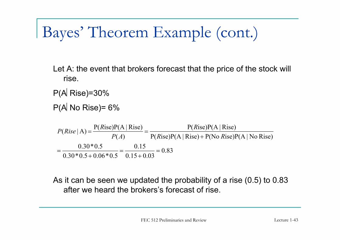
Bayes’ Theorem Example (cont.)
Let A: the event that brokers forecast that the price of the stock will
rise.
P(ARise)=30%
P(ANo Rise)= 6%
As it can be seen we updated the probability of a rise (0.5) to 0.83
after we heard the brokers’s forecast of rise.
83.003.015.0
15.0
5.0*06.05.0*30.0
5.0*30.0
Rise) No|ise)P(A P(NoRise)|ise)P(AP(
Rise)|ise)P(AP(
)(
Rise)|ise)P(AP(A)|(
=+
=+
=
+==
RR
R
AP
RRiseP
FEC 512 Preliminaries and Review Lecture 1-44
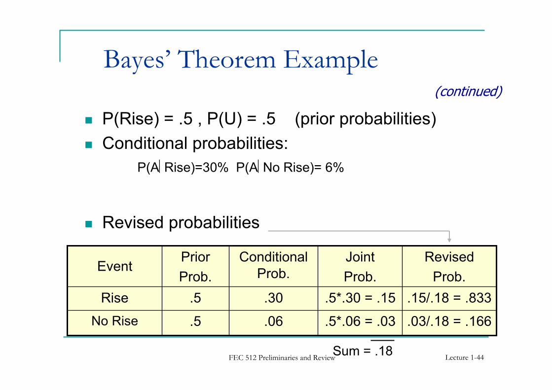
� P(Rise) = .5 , P(U) = .5 (prior probabilities)
� Conditional probabilities:
P(ARise)=30% P(ANo Rise)= 6%
� Revised probabilities
Bayes’ Theorem Example
.03/.18 = .166.5*.06 = .03.06.5No Rise
.15/.18 = .833.5*.30 = .15.30.5Rise
Revised
Prob.
Joint
Prob.
Conditional
Prob.
Prior
Prob.Event
Sum = .18
(continued)
FEC 512 Preliminaries and Review Lecture 1-45
Importance of Bayes Law
� We update our beliefs in light of new
information.
� Revising beliefs after receiving additional info
is smth that humans do poorly without the
help of mathematics.
� There is a tendency to put either too little or
too much emphasis on new info
� This problem can be mitigated by using
Bayes’ Law.
FEC 512 Preliminaries and Review Lecture 1-46
For Further Study
� For Topic I:Ruppert D. (2004), Statistics and
Finance, Springer.
� For Topic II:Groebner D.F. et al.(2008)
Business Statistics.
Related Documents