Intelligent Data Analysis 1 (1997) 131–156 www.elsevier.com/locate/ida Feature Selection for Classification M. Dash 1 , H. Liu 2 Department of Information Systems & Computer Science, National University of Singapore, Singapore 119260 Received 24 January 1997; revised 3 March 1997; accepted 21 March 1997 Abstract Feature selection has been the focus of interest for quite some time and much work has been done. With the creation of huge databases and the consequent requirements for good machine learning techniques, new problems arise and novel approaches to feature selection are in demand. This survey is a comprehensive overview of many existing methods from the 1970’s to the present. It identifies four steps of a typical feature selection method, and categorizes the different existing methods in terms of generation procedures and evaluation functions, and reveals hitherto unattempted combinations of generation procedures and evaluation functions. Representative methods are chosen from each category for detailed explanation and discussion via example. Benchmark datasets with different characteristics are used for comparative study. The strengths and weaknesses of different methods are explained. Guidelines for applying feature selection methods are given based on data types and domain characteristics. This survey identifies the future research areas in feature selection, introduces newcomers to this field, and paves the way for practitioners who search for suitable methods for solving domain-specific real-world applications. (Intelligent Data Analysis, Vol. 1, no. 3, http:llwww.elsevier.com/locate/ida) 1997 Elsevier Science B.V. All rights reserved. Keywords: Feature selection; Classification; Framework 1. Introduction The majority of real-world classification problems require supervised learning where the underlying class probabilities and class-conditional probabilities are unknown, and each instance is associated with a class label. In real-world situations, relevant features are often unknown a priori. Therefore, many candidate features are introduced to better represent the domain. Unfortunately many of these are either partially or completely irrelevant/redundant to the target concept. A relevant feature is neither irrelevant nor redundant to the target concept; an irrelevant feature does not affect the target concept in any way, and a redundant feature does not add anything new to the target concept [21]. In many applications, the size of a dataset is so large that learning might not work as well before removing these unwanted features. Reducing the number of irrelevant/redundant features drastically reduces the running time of a learning 1 E-mail: [email protected]. 2 E-mail: [email protected]. 1088-467X/97/$17.00 1997 Elsevier Science B.V. All rights reserved. PII:S1088-467X(97)00008-5

Welcome message from author
This document is posted to help you gain knowledge. Please leave a comment to let me know what you think about it! Share it to your friends and learn new things together.
Transcript
Intelligent Data Analysis 1 (1997) 131–156www.elsevier.com/locate/ida
Feature Selection for Classification
M. Dash1, H. Liu 2
Department of Information Systems & Computer Science, National University of Singapore, Singapore 119260
Received 24 January 1997; revised 3 March 1997; accepted 21 March 1997
Abstract
Feature selection has been the focus of interest for quite some time and much work has been done. With the creation of hugedatabases and the consequent requirements for good machine learning techniques, new problems arise and novel approachesto feature selection are in demand. This survey is a comprehensive overview of many existing methods from the 1970’s to thepresent. It identifies four steps of a typical feature selection method, and categorizes the different existing methods in termsof generation procedures and evaluation functions, and reveals hitherto unattempted combinations of generation proceduresand evaluation functions. Representative methods are chosen from each category for detailed explanation and discussion viaexample. Benchmark datasets with different characteristics are used for comparative study. The strengths and weaknesses ofdifferent methods are explained. Guidelines for applying feature selection methods are given based on data types and domaincharacteristics. This survey identifies the future research areas in feature selection, introduces newcomers to this field, and pavesthe way for practitioners who search for suitable methods for solving domain-specific real-world applications. (Intelligent DataAnalysis, Vol. 1, no. 3, http:llwww.elsevier.com/locate/ida) 1997 Elsevier Science B.V. All rights reserved.
Keywords:Feature selection; Classification; Framework
1. Introduction
The majority of real-world classification problems require supervised learning where the underlyingclass probabilities and class-conditional probabilities are unknown, and each instance is associated witha class label. In real-world situations, relevant features are often unknowna priori. Therefore, manycandidate features are introduced to better represent the domain. Unfortunately many of these are eitherpartially or completely irrelevant/redundant to the target concept. A relevant feature is neither irrelevantnor redundant to the target concept; an irrelevant feature does not affect the target concept in any way,and a redundant feature does not add anything new to the target concept [21]. In many applications, thesize of a dataset is so large that learning might not work as well before removing these unwanted features.Reducing the number of irrelevant/redundant features drastically reduces the running time of a learning
1 E-mail: [email protected] E-mail: [email protected].
1088-467X/97/$17.00 1997 Elsevier Science B.V. All rights reserved.PII: S1088-467X(97)00008-5
132 M. Dash, H. Liu / Intelligent Data Analysis 1 (1997) 131–156
algorithm and yields a more general concept. This helps in getting a better insight into the underlyingconcept of a real-world classification problem [23,24].Feature selectionmethods try to pick a subset offeatures that are relevant to the target concept.
Feature selection is defined by many authors by looking at it from various angles. But as expected,many of those are similar in intuition and/or content. The following lists those that are conceptuallydifferent and cover a range of definitions.
1. Idealized: find the minimally sized feature subset that is necessary and sufficient to the targetconcept [22].
2. Classical: select a subset ofM features from a set ofN features,M < N , such that the value of acriterion function is optimized over all subsets of sizeM [34].
3. Improving Prediction accuracy: the aim of feature selection is to choose a subset of features forimproving prediction accuracy or decreasing the size of the structure without significantly decreasingprediction accuracy of the classifier built using only the selected features [24].
4. Approximating original class distribution: the goal of feature selection is to select a small subsetsuch that the resulting class distribution, given only the values for the selected features, is as close aspossible to the original class distribution given all feature values [24].
Notice that the third definition emphasizes the prediction accuracy of a classifier, built using only theselected features, whereas the last definition emphasizes the class distribution given the training dataset.These two are quite different conceptually. Hence, our definition considers both factors.
Feature selection attempts to select the minimally sized subset of features according to the followingcriteria. The criteria can be:
1. the classification accuracy does not significantly decrease; and2. the resulting class distribution, given only the values for the selected features, is as close as possible
to the original class distribution, given all features.
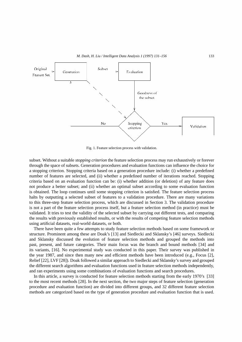
Ideally, feature selection methods search through the subsets of features, and try to find the bestone among the competing 2N candidate subsets according to some evaluation function. However thisprocedure is exhaustive as it tries to find only the best one. It may be too costly and practically prohibitive,even for a medium-sized feature set size (N ). Other methods based on heuristic or random searchmethods attempt to reduce computational complexity by compromising performance. These methodsneed a stopping criterion to prevent an exhaustive search of subsets. In our opinion, there are four basicsteps in a typical feature selection method (see Figure 1):
1. ageneration procedureto generate the next candidate subset;2. an evaluation functionto evaluate the subset under examination;3. astopping criterionto decide when to stop; and4. avalidation procedureto check whether the subset is valid.
Thegeneration procedureis asearch procedure[46,26]. Basically, it generates subsets of features forevaluation. The generation procedure can start: (i) with no features, (ii) with all features, or (iii) witha random subset of features. In the first two cases, features are iteratively added or removed, whereasin the last case, features are either iteratively added or removed or produced randomly thereafter [26].An evaluation functionmeasures the goodness of a subset produced by some generation procedure, andthis value is compared with the previous best. If it is found to be better, then it replaces the previous best
M. Dash, H. Liu / Intelligent Data Analysis 1 (1997) 131–156 133
Fig. 1. Feature selection process with validation.
subset. Without a suitablestopping criterionthe feature selection process may run exhaustively or foreverthrough the space of subsets. Generation procedures and evaluation functions can influence the choice fora stopping criterion. Stopping criteria based on a generation procedure include: (i) whether a predefinednumber of features are selected, and (ii) whether a predefined number of iterations reached. Stoppingcriteria based on an evaluation function can be: (i) whether addition (or deletion) of any feature doesnot produce a better subset; and (ii) whether an optimal subset according to some evaluation functionis obtained. The loop continues until some stopping criterion is satisfied. The feature selection processhalts by outputting a selected subset of features to a validation procedure. There are many variationsto this three-step feature selection process, which are discussed in Section 3. The validation procedureis not a part of the feature selection process itself, but a feature selection method (in practice) must bevalidated. It tries to test the validity of the selected subset by carrying out different tests, and comparingthe results with previously established results, or with the results of competing feature selection methodsusing artificial datasets, real-world datasets, or both.
There have been quite a few attempts to study feature selection methods based on some framework orstructure. Prominent among these are Doak’s [13] and Siedlecki and Sklansky’s [46] surveys. Siedleckiand Sklansky discussed the evolution of feature selection methods and grouped the methods intopast, present, and future categories. Their main focus was the branch and bound methods [34] andits variants, [16]. No experimental study was conducted in this paper. Their survey was published inthe year 1987, and since then many new and efficient methods have been introduced (e.g., Focus [2],Relief [22], LVF [28]). Doak followed a similar approach to Siedlecki and Sklansky’s survey and groupedthe different search algorithms and evaluation functions used in feature selection methods independently,and ran experiments using some combinations of evaluation functions and search procedures.
In this article, a survey is conducted for feature selection methods starting from the early 1970’s [33]to the most recent methods [28]. In the next section, the two major steps of feature selection (generationprocedure and evaluation function) are divided into different groups, and 32 different feature selectionmethods are categorized based on the type of generation procedure and evaluation function that is used.
134 M. Dash, H. Liu / Intelligent Data Analysis 1 (1997) 131–156
This framework helps in finding the unexplored combinations of generation procedures and evaluationfunctions. In Section 3 we briefly discuss the methods under each category, and select a representativemethod for a detailed description using a simple dataset. Section 4 describes an empirical comparisonof the representative methods using three artificial datasets suitably chosen to highlight their benefitsand limitations. Section 5 consists of discussions on various data set characteristics that influence thechoice of a suitable feature selection method, and some guidelines, regarding how to choose a featureselection method for an application at hand, are given based on a number of criterial extracted from thesecharacteristics of data. This paper concludes in Section 6 with further discussions on future researchbased on the findings of Section 2. Our objective is that this article will assist in finding better featureselection methods for given applications.
2. Study of Feature Selection Methods
In this section we categorize the two major steps of feature selection: generation procedure andevaluation function. The different types of evaluation functions are compared based on a number ofcriteria. A framework is presented in which a total of 32 methods are grouped based on the types ofgeneration procedure and evaluation function used in them.
2.1. Generation Procedures
If the original feature set containsN number of features, then the total number of competing candidatesubsets to be generated is 2N. This is a huge number even for medium-sizedN . There are differentapproaches for solving this problem, namely:complete, heuristic, and random.
2.1.1. CompleteThis generation procedure does a complete search for the optimal subset according to the evaluation
function used. An exhaustive search is complete. However, Schlimmer [43] argues that “just because thesearch must be complete does not mean that it must be exhaustive.” Different heuristic functions are usedto reduce the search without jeopardizing the chances of finding the optimal subset. Hence, although theorder of the search space is O(2N ), a fewer subsets are evaluated. The optimality of the feature subset,according to the evaluation function, is guaranteed because the procedure can backtrack. Backtrackingcan be done using various techniques, such as: branch and bound, best first search, and beam search.
2.1.2. HeuristicIn each iteration of this generation procedure, all remaining features yet to be selected (rejected) are
considered for selection (rejection). There are many variations to this simple process, but generation ofsubsets is basically incremental (either increasing or decreasing). The order of the search space is O(N2)or less; some exceptions are Relief [22], DTM [9] that are discussed in detail in the next section. Theseprocedures are very simple to implement and very fast in producing results, because the search space isonly quadratic in terms of the number of features.
2.1.3. RandomThis generation procedure is rather new in its use in feature selection methods compared to the other
two categories. Although the search space is O(2N ), but these methods typically search fewer number of
M. Dash, H. Liu / Intelligent Data Analysis 1 (1997) 131–156 135
subsets than 2N by setting a maximum number of iterations possible. Optimality of the selected subsetdepends on the resources available. Each random generation procedure would require values of someparameters. Assignment of suitable values to these parameters is an important task for achieving goodresults.
2.2. Evaluation Functions
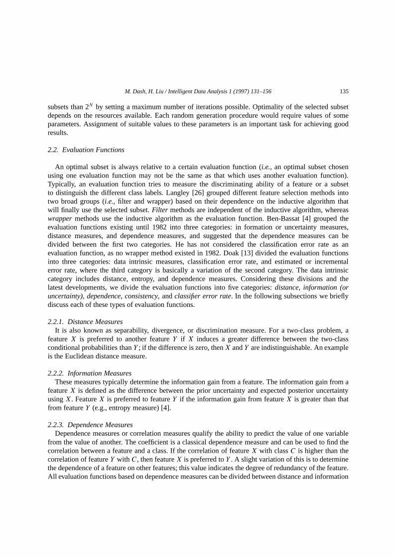
An optimal subset is always relative to a certain evaluation function (i.e., an optimal subset chosenusing one evaluation function may not be the same as that which uses another evaluation function).Typically, an evaluation function tries to measure the discriminating ability of a feature or a subsetto distinguish the different class labels. Langley [26] grouped different feature selection methods intotwo broad groups (i.e., filter and wrapper) based on their dependence on the inductive algorithm thatwill finally use the selected subset.Filter methods are independent of the inductive algorithm, whereaswrapper methods use the inductive algorithm as the evaluation function. Ben-Bassat [4] grouped theevaluation functions existing until 1982 into three categories: in formation or uncertainty measures,distance measures, and dependence measures, and suggested that the dependence measures can bedivided between the first two categories. He has not considered the classification error rate as anevaluation function, as no wrapper method existed in 1982. Doak [13] divided the evaluation functionsinto three categories: data intrinsic measures, classification error rate, and estimated or incrementalerror rate, where the third category is basically a variation of the second category. The data intrinsiccategory includes distance, entropy, and dependence measures. Considering these divisions and thelatest developments, we divide the evaluation functions into five categories:distance, information (oruncertainty), dependence, consistency, andclassifier error rate. In the following subsections we brieflydiscuss each of these types of evaluation functions.
2.2.1. Distance MeasuresIt is also known as separability, divergence, or discrimination measure. For a two-class problem, a
featureX is preferred to another featureY if X induces a greater difference between the two-classconditional probabilities thanY ; if the difference is zero, thenX andY are indistinguishable. An exampleis the Euclidean distance measure.
2.2.2. Information MeasuresThese measures typically determine the information gain from a feature. The information gain from a
featureX is defined as the difference between the prior uncertainty and expected posterior uncertaintyusingX. FeatureX is preferred to featureY if the information gain from featureX is greater than thatfrom featureY (e.g., entropy measure) [4].
2.2.3. Dependence MeasuresDependence measures or correlation measures qualify the ability to predict the value of one variable
from the value of another. The coefficient is a classical dependence measure and can be used to find thecorrelation between a feature and a class. If the correlation of featureX with classC is higher than thecorrelation of featureY with C, then featureX is preferred toY . A slight variation of this is to determinethe dependence of a feature on other features; this value indicates the degree of redundancy of the feature.All evaluation functions based on dependence measures can be divided between distance and information

136 M. Dash, H. Liu / Intelligent Data Analysis 1 (1997) 131–156
Table 1A Comparison of Evaluation Functions
Evaluation Function Generality Time Complexity Accuracy
Distance Measure Yes Low –
Information Measure Yes Low –
Dependence Measure Yes Low –
Consistency Measure Yes Moderate –
Classifier Error Rate No High Very High
measures. But, these are still kept as a separate category, because conceptually, they represent a differentviewpoint [4]. More about the above three measures can be found in Ben-Basset’s [4] survey.
2.2.4. Consistency MeasuresThese measures are rather new and have been in much focus recently. These are characteristically
different from other measures, because of their heavy reliance on the training dataset and the use of theMin-Features bias in selecting a subset of features [3]. Min-Features bias prefers consistent hypothesesdefinable over as few features as possible. More about this bias is discussed in Section 3.6. Thesemeasures find out the minimally sized subset that satisfies the acceptable inconsistency rate, that is usuallyset by the user.
2.2.5. Classifier Error Rate MeasuresThe methods using this type of evaluation function are called “wrapper methods”, (i.e., the classifier is
the evaluation function). As the features are selected using the classifier that later on uses these selectedfeatures in predicting the class labels of unseen instances, the accuracy level is very high althoughcomputationally quite costly [21].
Table 1 shows a comparison of various evaluation functions irrespective of the type of generationprocedure used. The different parameters used for the comparison are:
1. generality: how suitable is the selected subset for different classifiers (not just for one classifier);2. time complexity: time taken for selecting the subset of features; and3. accuracy: how accurate is the prediction using the selected subset.
The ‘–’ in the last column means that nothing can be concluded about the accuracy of thecorresponding evaluation function. Except ‘classifier error rate,’ the accuracy of all other evaluationfunctions depends on the data set and the classifier (for classification after feature selection) used. Theresults in Table 1 show a non-surprising trend (i.e., the more time spent, the higher the accuracy). Thetable also tells us which measure should be used under different circumstances, for example, with timeconstraints, given several classifiers to choose from, classifier error rate should not be selected as anevaluation function.
2.3. The Framework
In this subsection, we suggest a framework on which the feature selection methods are categorized.Generation procedures and evaluation functions are considered as two dimensions, and each method is
M. Dash, H. Liu / Intelligent Data Analysis 1 (1997) 131–156 137
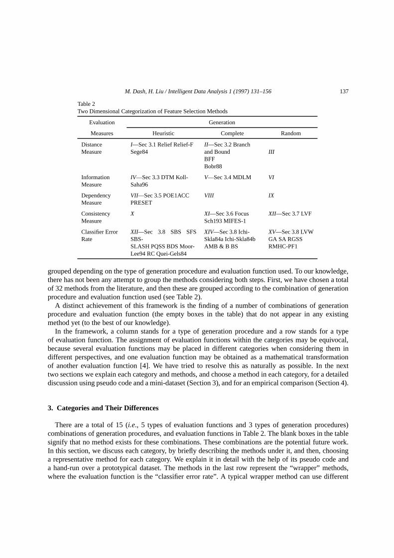
Table 2Two Dimensional Categorization of Feature Selection Methods
Evaluation Generation
Measures Heuristic Complete Random
DistanceMeasure
I—Sec 3.1 Relief Relief-FSege84
II—Sec 3.2 Branchand BoundBFFBobr88
III
InformationMeasure
IV—Sec 3.3 DTM Koll-Saha96
V—Sec 3.4 MDLM VI
DependencyMeasure
VII—Sec 3.5 POE1ACCPRESET
VIII IX
ConsistencyMeasure
X XI—Sec 3.6 FocusSch193 MIFES-1
XII—Sec 3.7 LVF
Classifier ErrorRate
XII—Sec 3.8 SBS SFSSBS-SLASH PQSS BDS Moor-Lee94 RC Quei-Gels84
XIV—Sec 3.8 Ichi-Skla84a Ichi-Skla84bAMB & B BS
XV—Sec 3.8 LVWGA SA RGSSRMHC-PF1
grouped depending on the type of generation procedure and evaluation function used. To our knowledge,there has not been any attempt to group the methods considering both steps. First, we have chosen a totalof 32 methods from the literature, and then these are grouped according to the combination of generationprocedure and evaluation function used (see Table 2).
A distinct achievement of this framework is the finding of a number of combinations of generationprocedure and evaluation function (the empty boxes in the table) that do not appear in any existingmethod yet (to the best of our knowledge).
In the framework, a column stands for a type of generation procedure and a row stands for a typeof evaluation function. The assignment of evaluation functions within the categories may be equivocal,because several evaluation functions may be placed in different categories when considering them indifferent perspectives, and one evaluation function may be obtained as a mathematical transformationof another evaluation function [4]. We have tried to resolve this as naturally as possible. In the nexttwo sections we explain each category and methods, and choose a method in each category, for a detaileddiscussion using pseudo code and a mini-dataset (Section 3), and for an empirical comparison (Section 4).
3. Categories and Their Differences
There are a total of 15 (i.e., 5 types of evaluation functions and 3 types of generation procedures)combinations of generation procedures, and evaluation functions in Table 2. The blank boxes in the tablesignify that no method exists for these combinations. These combinations are the potential future work.In this section, we discuss each category, by briefly describing the methods under it, and then, choosinga representative method for each category. We explain it in detail with the help of its pseudo code anda hand-run over a prototypical dataset. The methods in the last row represent the “wrapper” methods,where the evaluation function is the “classifier error rate”. A typical wrapper method can use different
138 M. Dash, H. Liu / Intelligent Data Analysis 1 (1997) 131–156
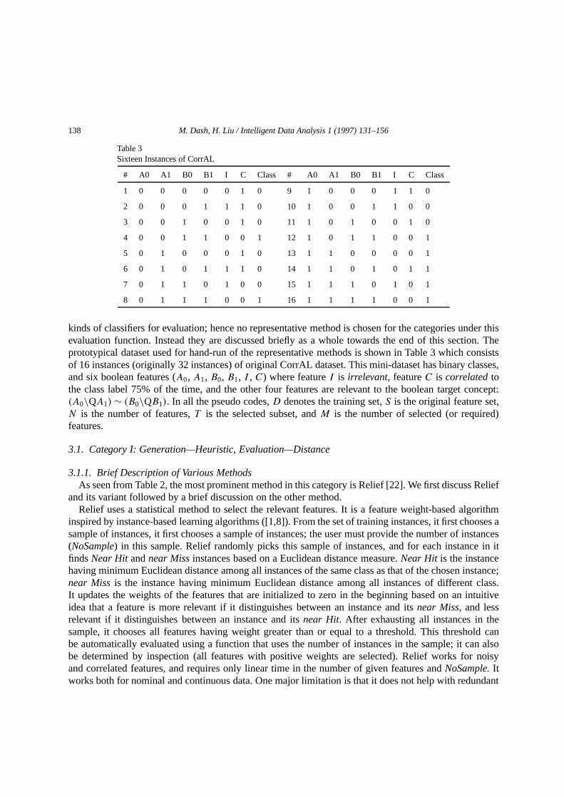
Table 3Sixteen Instances of CorrAL
# A0 A1 B0 B1 I C Class # A0 A1 B0 B1 I C Class
1 0 0 0 0 0 1 0 9 1 0 0 0 1 1 0
2 0 0 0 1 1 1 0 10 1 0 0 1 1 0 0
3 0 0 1 0 0 1 0 11 1 0 1 0 0 1 0
4 0 0 1 1 0 0 1 12 1 0 1 1 0 0 1
5 0 1 0 0 0 1 0 13 1 1 0 0 0 0 1
6 0 1 0 1 1 1 0 14 1 1 0 1 0 1 1
7 0 1 1 0 1 0 0 15 1 1 1 0 1 0 1
8 0 1 1 1 0 0 1 16 1 1 1 1 0 0 1
kinds of classifiers for evaluation; hence no representative method is chosen for the categories under thisevaluation function. Instead they are discussed briefly as a whole towards the end of this section. Theprototypical dataset used for hand-run of the representative methods is shown in Table 3 which consistsof 16 instances (originally 32 instances) of original CorrAL dataset. This mini-dataset has binary classes,and six boolean features (A0, A1, B0, B1, I , C) where featureI is irrelevant, featureC is correlatedtothe class label 75% of the time, and the other four features are relevant to the boolean target concept:(A0\QA1)∼ (B0\QB1). In all the pseudo codes,D denotes the training set,S is the original feature set,N is the number of features,T is the selected subset, andM is the number of selected (or required)features.
3.1. Category I: Generation—Heuristic, Evaluation—Distance
3.1.1. Brief Description of Various MethodsAs seen from Table 2, the most prominent method in this category is Relief [22]. We first discuss Relief
and its variant followed by a brief discussion on the other method.Relief uses a statistical method to select the relevant features. It is a feature weight-based algorithm
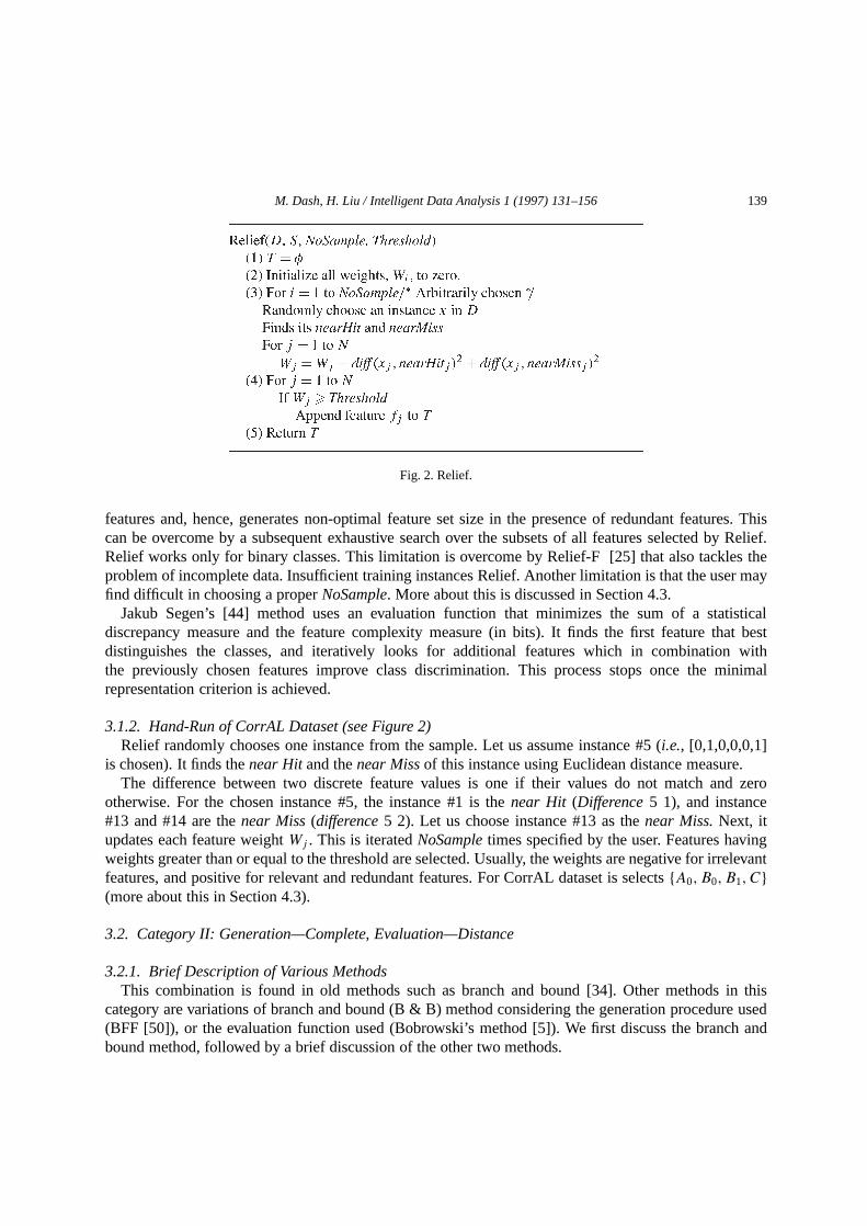
inspired by instance-based learning algorithms ([1,8]). From the set of training instances, it first chooses asample of instances, it first chooses a sample of instances; the user must provide the number of instances(NoSample) in this sample. Relief randomly picks this sample of instances, and for each instance in itfindsNear Hit andnear Missinstances based on a Euclidean distance measure.Near Hit is the instancehaving minimum Euclidean distance among all instances of the same class as that of the chosen instance;near Missis the instance having minimum Euclidean distance among all instances of different class.It updates the weights of the features that are initialized to zero in the beginning based on an intuitiveidea that a feature is more relevant if it distinguishes between an instance and itsnear Miss, and lessrelevant if it distinguishes between an instance and itsnear Hit. After exhausting all instances in thesample, it chooses all features having weight greater than or equal to a threshold. This threshold canbe automatically evaluated using a function that uses the number of instances in the sample; it can alsobe determined by inspection (all features with positive weights are selected). Relief works for noisyand correlated features, and requires only linear time in the number of given features andNoSample.Itworks both for nominal and continuous data. One major limitation is that it does not help with redundant
M. Dash, H. Liu / Intelligent Data Analysis 1 (1997) 131–156 139
Fig. 2. Relief.
features and, hence, generates non-optimal feature set size in the presence of redundant features. Thiscan be overcome by a subsequent exhaustive search over the subsets of all features selected by Relief.Relief works only for binary classes. This limitation is overcome by Relief-F [25] that also tackles theproblem of incomplete data. Insufficient training instances Relief. Another limitation is that the user mayfind difficult in choosing a properNoSample. More about this is discussed in Section 4.3.
Jakub Segen’s [44] method uses an evaluation function that minimizes the sum of a statisticaldiscrepancy measure and the feature complexity measure (in bits). It finds the first feature that bestdistinguishes the classes, and iteratively looks for additional features which in combination withthe previously chosen features improve class discrimination. This process stops once the minimalrepresentation criterion is achieved.
3.1.2. Hand-Run of CorrAL Dataset (see Figure 2)Relief randomly chooses one instance from the sample. Let us assume instance #5 (i.e., [0,1,0,0,0,1]
is chosen). It finds thenear Hitand thenear Missof this instance using Euclidean distance measure.The difference between two discrete feature values is one if their values do not match and zero
otherwise. For the chosen instance #5, the instance #1 is thenear Hit (Difference5 1), and instance#13 and #14 are thenear Miss(difference5 2). Let us choose instance #13 as thenear Miss.Next, itupdates each feature weightWj . This is iteratedNoSampletimes specified by the user. Features havingweights greater than or equal to the threshold are selected. Usually, the weights are negative for irrelevantfeatures, and positive for relevant and redundant features. For CorrAL dataset is selects{A0,B0,B1,C}(more about this in Section 4.3).
3.2. Category II: Generation—Complete, Evaluation—Distance
3.2.1. Brief Description of Various MethodsThis combination is found in old methods such as branch and bound [34]. Other methods in this
category are variations of branch and bound (B & B) method considering the generation procedure used(BFF [50]), or the evaluation function used (Bobrowski’s method [5]). We first discuss the branch andbound method, followed by a brief discussion of the other two methods.
140 M. Dash, H. Liu / Intelligent Data Analysis 1 (1997) 131–156
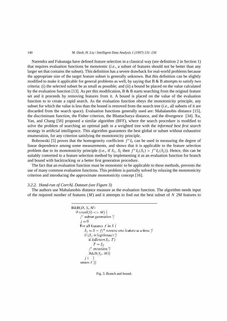
Narendra and Fukunaga have defined feature selection in a classical way (see definition 2 in Section 1)that requires evaluation functions be monotonic (i.e., a subset of features should not be better than anylarger set that contains the subset). This definition has a severe drawback for real-world problems becausethe appropriate size of the target feature subset is generally unknown. But this definition can be slightlymodified to make it applicable for general problems as well, by saying that B & B attempts to satisfy twocriteria: (i) the selected subset be as small as possible; and (ii) a bound be placed on the value calculatedby the evaluation function [13]. As per this modification, B & B starts searching from the original featureset and it proceeds by removing features from it. A bound is placed on the value of the evaluationfunction to to create a rapid search. As the evaluation function obeys the monotonicity principle, anysubset for which the value is less than the bound is removed from the search tree (i.e., all subsets of it arediscarded from the search space). Evaluation functions generally used are: Mahalanobis distance [15],the discriminant function, the Fisher criterion, the Bhattacharya distance, and the divergence [34]. Xu,Yan, and Chang [50] proposed a similar algorithm (BFF), where the search procedure is modified tosolve the problem of searching an optimal path in a weighted tree with theinformed best first searchstrategy in artificial intelligence. This algorithm guarantees the best global or subset without exhaustiveenumeration, for any criterion satisfying the monotonicity principle.
Bobrowski [5] proves that the homogeneity coefficientf ∗Ik can be used in measuring the degree oflinear dependence among some measurements, and shows that it is applicable to the feature selectionproblem due to its monotonicity principle (i.e., if S1, S2 thenf ∗Ik(S1) > f
∗Ik(S2)). Hence, this can besuitably converted to a feature selection method by implementing it as an evaluation function for branchand bound with backtracking or a better first generation procedure.
The fact that an evaluation function must be monotonic to be applicable to these methods, prevents theuse of many common evaluation functions. This problem is partially solved by relaxing the monotonicitycriterion and introducing the approximate monotonicity concept [16].
3.2.2. Hand-run of CorrAL Dataset (see Figure 3)The authors use Mahalanobis distance measure as the evaluation function. The algorithm needs input
of the required number of features (M) and it attempts to find out the best subset ofN 2M features to
Fig. 3. Branch and bound.
M. Dash, H. Liu / Intelligent Data Analysis 1 (1997) 131–156 141
Fig. 4. Decision tree method (DTM).
reject. It begins with the full set of featuresS0, removes one feature fromSljˆ21 in turn to generate subsetsSlj , wherel is the current level andj specifies different subsets at thelth level. If U(Slj ). U(S
ljˆ21), Slj
stops growing (its branch is pruned), otherwise, it grows to levell 1 1, i.e., one more feature will beremoved. If for the CorrAL dataset,M is set to 4, then subset (A0, A1, B0, I ) is selected as the bestsubset of 4 features.
3.3. Category IV: Generation—Heuristic, Evaluation—Information
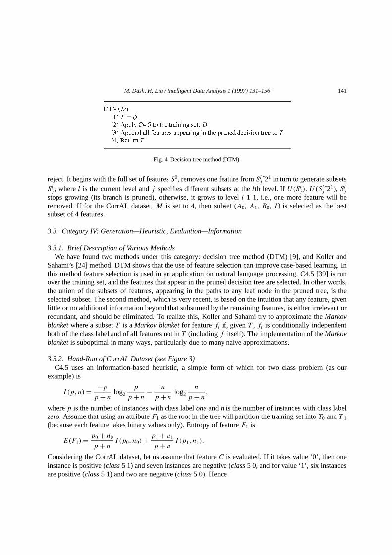
3.3.1. Brief Description of Various MethodsWe have found two methods under this category: decision tree method (DTM) [9], and Koller and
Sahami’s [24] method. DTM shows that the use of feature selection can improve case-based learning. Inthis method feature selection is used in an application on natural language processing. C4.5 [39] is runover the training set, and the features that appear in the pruned decision tree are selected. In other words,the union of the subsets of features, appearing in the paths to any leaf node in the pruned tree, is theselected subset. The second method, which is very recent, is based on the intuition that any feature, givenlittle or no additional information beyond that subsumed by the remaining features, is either irrelevant orredundant, and should be eliminated. To realize this, Koller and Sahami try to approximate theMarkovblanketwhere a subsetT is aMarkov blanketfor featurefi if, given T , fi is conditionally independentboth of the class label and of all features not inT (includingfi itself). The implementation of theMarkovblanketis suboptimal in many ways, particularly due to many naive approximations.
3.3.2. Hand-Run of CorrAL Dataset (see Figure 3)C4.5 uses an information-based heuristic, a simple form of which for two class problem (as our
example) is
I (p,n)= −pp+ n log2
p
p+ n −n
p+ n log2n
p+ n,wherep is the number of instances with class labeloneandn is the number of instances with class labelzero.Assume that using an attributeF1 as the root in the tree will partition the training set intoT0 andT 1
(because each feature takes binary values only). Entropy of featureF1 is
E(F1)= p0+ n0
p+ n I (p0, n0)+ p1+ n1
p+ n I (p1, n1).
Considering the CorrAL dataset, let us assume that featureC is evaluated. If it takes value ‘0’, then oneinstance is positive (class5 1) and seven instances are negative (class5 0, and for value ‘1’, six instancesare positive (class5 1) and two are negative (class5 0). Hence

142 M. Dash, H. Liu / Intelligent Data Analysis 1 (1997) 131–156
E(C)= 1+ 7
16I (1,7)+ 6+ 2
16I (6,2)
is 0.552421. In fact this value is minimum among all features, andC is selected as the root of thedecision tree. The original training set of sixteen instances is divided into two nodes, each representingeight instances using featureC. For these two nodes, again features having the least entropy are selected,and so on. This process halts when each partition contains instances of a single class, or until no testoffers any improvement. The decision tree constructed, thus is pruned basically to avoid over-fitting.DTM chooses all features appearing in the pruned decision tree (i.e.,A0, A1, B0, B1, C).
3.4. Category V: Generation—Complete, Evaluation—Information
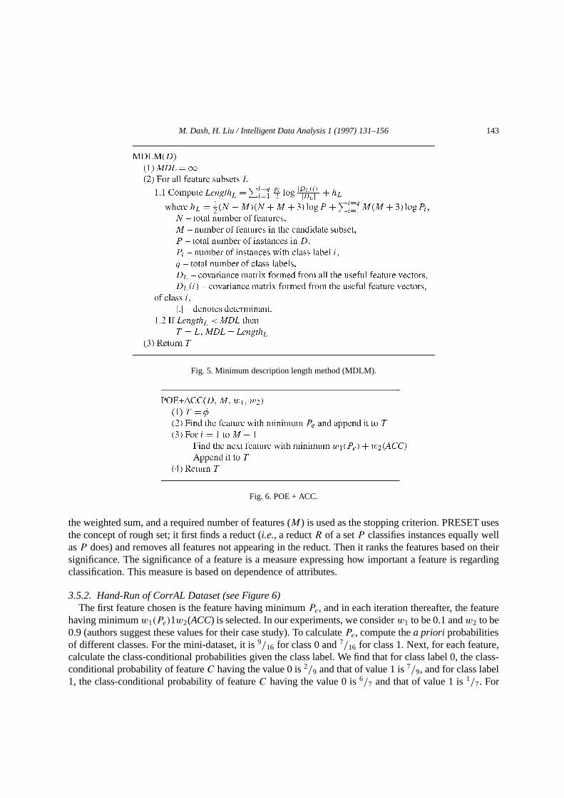
Under this category we found Minimum Description Length Method (MDLM) [45]. In this method,the authors have attempted to eliminate alluseless(irrelevant and/or redundant) features. According tothe authors, if the features in a subsetV can be expressed as a fixed non-class-dependent functionF ofthe features in another subsetU , then once the values of the features in subsetU are known, the featuresubsetV becomes useless. For feature selection,U andV together make up the complete feature setand one has the task of separating them. To solve this, the authors use the minimum description lengthcriterion (MDLC) introduced by Rissanen [40]. They formulated an expression that can be interpretedas the number of bits required to transmit the classes of the instances, the optimal parameters, the usefulfeatures, and (finally) the useless features. The algorithm exhaustively searches all the possible subsets(2N ) and outputs the subset satisfying MDLC. This method can find all the useful features and only thoseof the observations are Gaussian. For non-Gaussian cases, it may not be able to find the useful features(more about this in Section 4.3).
3.4.1. Hand-Run of CorrAL DatasetAs seen in Figure 5, MDLM is basically the evaluation of an equation that represents the description
length given the candidate subset of features. The actual implementation suggested by the authors is asfollows. Calculate the covariance matrices of the whole feature vectors for all classes and for each classseparately. The covariance matrix for useful subsets are obtained as sub-matrices of these. Determinethe determinants of the sub-matricesDL(i) andDL for equation as shown in Figure 5, and find out thesubset having minimum description length. For the CorrAL dataset the chosen feature subset is{C} witha minimum description length of 119.582.
3.5. Category VII: Generation—Heuristic, Evaluation—Dependence
3.5.1. Brief Description of Various MethodsWe found POE1ACC (Probability of ERROR & Average Correlation Coefficient) method [33] and
PRESET [31] under this combination. As many as seven techniques of feature selection are presentedin POE1ACC, but we choose the last (i.e., seventh) method, because the authors consider this to be themost important among the seven.
In this method, the first feature selected is the feature with the smallest probability of error (Pe).The next feature selected is the feature that produces the minimum weighted sum ofPe and averagecorrelation coefficient (ACC), and so on. ACC is the mean of the correlation coefficients of the candidatefeature with the features previously selected at that point. This method can rank all the features based on
M. Dash, H. Liu / Intelligent Data Analysis 1 (1997) 131–156 143
Fig. 5. Minimum description length method (MDLM).
Fig. 6. POE + ACC.
the weighted sum, and a required number of features (M) is used as the stopping criterion. PRESET usesthe concept of rough set; it first finds a reduct (i.e., a reductR of a setP classifies instances equally wellasP does) and removes all features not appearing in the reduct. Then it ranks the features based on theirsignificance. The significance of a feature is a measure expressing how important a feature is regardingclassification. This measure is based on dependence of attributes.
3.5.2. Hand-Run of CorrAL Dataset (see Figure 6)The first feature chosen is the feature having minimumPe, and in each iteration thereafter, the feature
having minimumw1(Pe)1w2(ACC) is selected. In our experiments, we considerw1 to be 0.1 andw2 to be0.9 (authors suggest these values for their case study). To calculatePe, compute thea priori probabilitiesof different classes. For the mini-dataset, it is9/16 for class 0 and7/16 for class 1. Next, for each feature,calculate the class-conditional probabilities given the class label. We find that for class label 0, the class-conditional probability of featureC having the value 0 is2/9 and that of value 1 is7/9, and for class label1, the class-conditional probability of featureC having the value 0 is6/7 and that of value 1 is1/7. For
144 M. Dash, H. Liu / Intelligent Data Analysis 1 (1997) 131–156
each feature value (e.g., featureC taking value 0), we find out the class label for the product ofa prioriclass probability and class-conditional probability given that the class label is maximum. When featureC takes the value 0, the prediction is class 1, and when featureC takes value 1, the prediction is class 0.For all instances, we count the number of mismatches between the actual and the predicted class values.FeatureC has3/16 fraction of mismatches (Pe). In fact, among all features,C has the leastPe and hence,is selected as the first feature. In the second step, correlations of all remaining features (A0, A1, B0, B1,I ) with featureC are calculated. Using the expressionw1(Pe)1w2(ACC) we find that featureA0 has theleast value among the five features and is chosen as the second feature. IfM (required number) is 4, thensubset (C, A0, B0, I ) is selected.
3.6. Category XI: Generation—Complete, Evaluation—Consistency
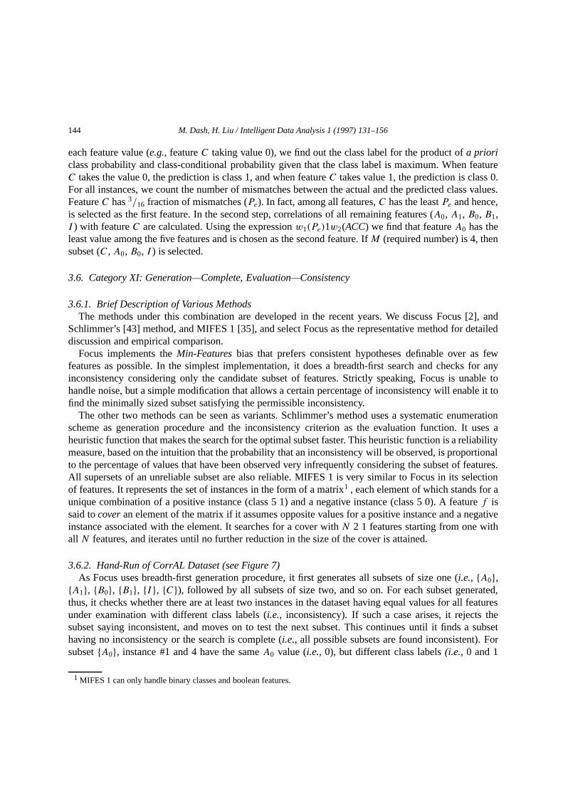
3.6.1. Brief Description of Various MethodsThe methods under this combination are developed in the recent years. We discuss Focus [2], and
Schlimmer’s [43] method, and MIFES 1 [35], and select Focus as the representative method for detaileddiscussion and empirical comparison.
Focus implements theMin-Featuresbias that prefers consistent hypotheses definable over as fewfeatures as possible. In the simplest implementation, it does a breadth-first search and checks for anyinconsistency considering only the candidate subset of features. Strictly speaking, Focus is unable tohandle noise, but a simple modification that allows a certain percentage of inconsistency will enable it tofind the minimally sized subset satisfying the permissible inconsistency.
The other two methods can be seen as variants. Schlimmer’s method uses a systematic enumerationscheme as generation procedure and the inconsistency criterion as the evaluation function. It uses aheuristic function that makes the search for the optimal subset faster. This heuristic function is a reliabilitymeasure, based on the intuition that the probability that an inconsistency will be observed, is proportionalto the percentage of values that have been observed very infrequently considering the subset of features.All supersets of an unreliable subset are also reliable. MIFES 1 is very similar to Focus in its selectionof features. It represents the set of instances in the form of a matrix1 , each element of which stands for aunique combination of a positive instance (class 5 1) and a negative instance (class 5 0). A featuref issaid tocoveran element of the matrix if it assumes opposite values for a positive instance and a negativeinstance associated with the element. It searches for a cover withN 2 1 features starting from one withall N features, and iterates until no further reduction in the size of the cover is attained.
3.6.2. Hand-Run of CorrAL Dataset (see Figure 7)As Focus uses breadth-first generation procedure, it first generates all subsets of size one (i.e., {A0},{A1}, {B0}, {B1}, {I }, {C}), followed by all subsets of size two, and so on. For each subset generated,thus, it checks whether there are at least two instances in the dataset having equal values for all featuresunder examination with different class labels (i.e., inconsistency). If such a case arises, it rejects thesubset saying inconsistent, and moves on to test the next subset. This continues until it finds a subsethaving no inconsistency or the search is complete (i.e., all possible subsets are found inconsistent). Forsubset{A0}, instance #1 and 4 have the sameA0 value (i.e., 0), but different class labels(i.e., 0 and 1
1 MIFES 1 can only handle binary classes and boolean features.
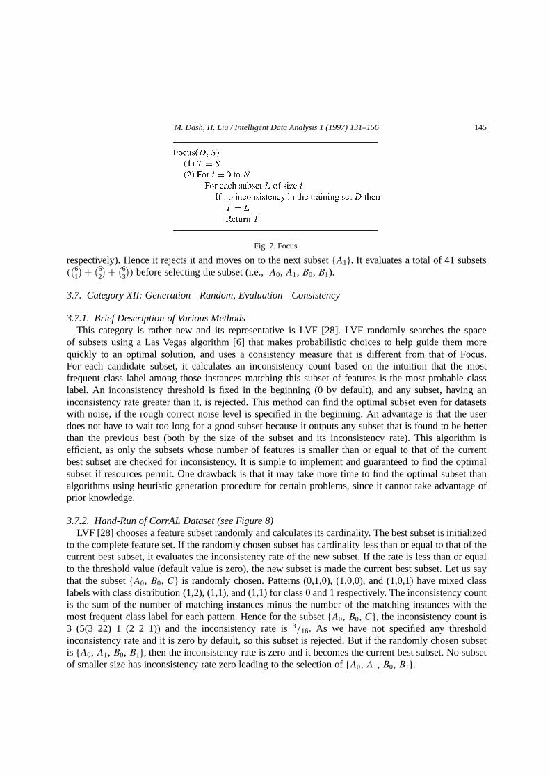
M. Dash, H. Liu / Intelligent Data Analysis 1 (1997) 131–156 145
Fig. 7. Focus.
respectively). Hence it rejects it and moves on to the next subset{A1}. It evaluates a total of 41 subsets((6
1
)+ (62)+ (63)) before selecting the subset (i.e.,A0, A1, B0, B1).
3.7. Category XII: Generation—Random, Evaluation—Consistency
3.7.1. Brief Description of Various MethodsThis category is rather new and its representative is LVF [28]. LVF randomly searches the space
of subsets using a Las Vegas algorithm [6] that makes probabilistic choices to help guide them morequickly to an optimal solution, and uses a consistency measure that is different from that of Focus.For each candidate subset, it calculates an inconsistency count based on the intuition that the mostfrequent class label among those instances matching this subset of features is the most probable classlabel. An inconsistency threshold is fixed in the beginning (0 by default), and any subset, having aninconsistency rate greater than it, is rejected. This method can find the optimal subset even for datasetswith noise, if the rough correct noise level is specified in the beginning. An advantage is that the userdoes not have to wait too long for a good subset because it outputs any subset that is found to be betterthan the previous best (both by the size of the subset and its inconsistency rate). This algorithm isefficient, as only the subsets whose number of features is smaller than or equal to that of the currentbest subset are checked for inconsistency. It is simple to implement and guaranteed to find the optimalsubset if resources permit. One drawback is that it may take more time to find the optimal subset thanalgorithms using heuristic generation procedure for certain problems, since it cannot take advantage ofprior knowledge.
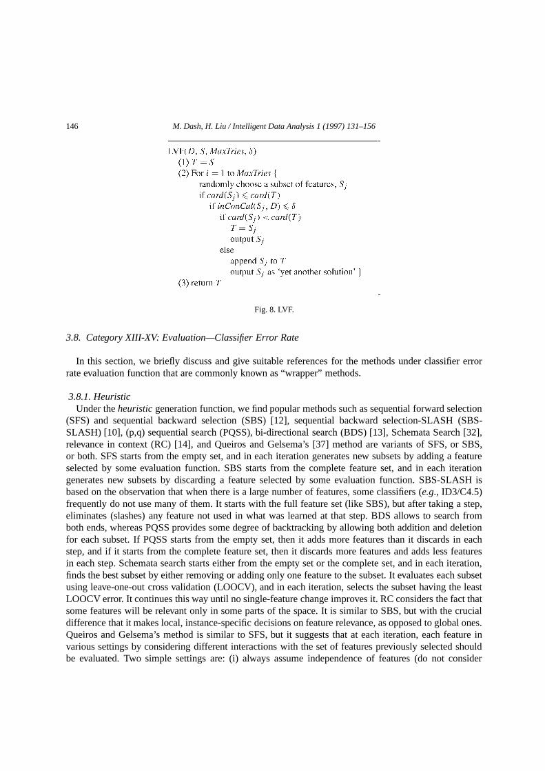
3.7.2. Hand-Run of CorrAL Dataset (see Figure 8)LVF [28] chooses a feature subset randomly and calculates its cardinality. The best subset is initialized
to the complete feature set. If the randomly chosen subset has cardinality less than or equal to that of thecurrent best subset, it evaluates the inconsistency rate of the new subset. If the rate is less than or equalto the threshold value (default value is zero), the new subset is made the current best subset. Let us saythat the subset{A0, B0, C} is randomly chosen. Patterns (0,1,0), (1,0,0), and (1,0,1) have mixed classlabels with class distribution (1,2), (1,1), and (1,1) for class 0 and 1 respectively. The inconsistency countis the sum of the number of matching instances minus the number of the matching instances with themost frequent class label for each pattern. Hence for the subset{A0, B0, C}, the inconsistency count is3 (5(3 22) 1 (2 2 1)) and the inconsistency rate is3/16. As we have not specified any thresholdinconsistency rate and it is zero by default, so this subset is rejected. But if the randomly chosen subsetis {A0, A1, B0, B1}, then the inconsistency rate is zero and it becomes the current best subset. No subsetof smaller size has inconsistency rate zero leading to the selection of{A0, A1, B0, B1}.
146 M. Dash, H. Liu / Intelligent Data Analysis 1 (1997) 131–156
Fig. 8. LVF.
3.8. Category XIII-XV: Evaluation—Classifier Error Rate
In this section, we briefly discuss and give suitable references for the methods under classifier errorrate evaluation function that are commonly known as “wrapper” methods.
3.8.1. HeuristicUnder theheuristicgeneration function, we find popular methods such as sequential forward selection
(SFS) and sequential backward selection (SBS) [12], sequential backward selection-SLASH (SBS-SLASH) [10], (p,q) sequential search (PQSS), bi-directional search (BDS) [13], Schemata Search [32],relevance in context (RC) [14], and Queiros and Gelsema’s [37] method are variants of SFS, or SBS,or both. SFS starts from the empty set, and in each iteration generates new subsets by adding a featureselected by some evaluation function. SBS starts from the complete feature set, and in each iterationgenerates new subsets by discarding a feature selected by some evaluation function. SBS-SLASH isbased on the observation that when there is a large number of features, some classifiers (e.g., ID3/C4.5)frequently do not use many of them. It starts with the full feature set (like SBS), but after taking a step,eliminates (slashes) any feature not used in what was learned at that step. BDS allows to search fromboth ends, whereas PQSS provides some degree of backtracking by allowing both addition and deletionfor each subset. If PQSS starts from the empty set, then it adds more features than it discards in eachstep, and if it starts from the complete feature set, then it discards more features and adds less featuresin each step. Schemata search starts either from the empty set or the complete set, and in each iteration,finds the best subset by either removing or adding only one feature to the subset. It evaluates each subsetusing leave-one-out cross validation (LOOCV), and in each iteration, selects the subset having the leastLOOCV error. It continues this way until no single-feature change improves it. RC considers the fact thatsome features will be relevant only in some parts of the space. It is similar to SBS, but with the crucialdifference that it makes local, instance-specific decisions on feature relevance, as opposed to global ones.Queiros and Gelsema’s method is similar to SFS, but it suggests that at each iteration, each feature invarious settings by considering different interactions with the set of features previously selected shouldbe evaluated. Two simple settings are: (i) always assume independence of features (do not consider
M. Dash, H. Liu / Intelligent Data Analysis 1 (1997) 131–156 147
the previously selected features), and (ii) never assume independence (consider the previously selectedfeatures). Bayesian classifier error rate as the evaluation function was used.
3.8.1. CompleteUnder completegeneration procedure, we find fourwrapper methods. Ichino and Sklansky have
devised two methods based on two different classifiers, namely: linear classifier [19] and boxclassifier [20]. In both methods, they solve the feature selection problem using zero-one integerprogramming [17]. Approximate monotonic branch and bound (AMB&B) was introduced to combat thedisadvantage of B&B by permitting evaluation functions that are not monotonic [16]. In it, the bound ofB&B is relaxed to generate subsets that appear below some subset violating the bound; but the selectedsubset should not violate the bound.Beam Search(BS), [13] is a type of best-first search that uses abounded queue to limit the scope of the search. The queue is ordered from best to worst with the bestsubsets at the front of the queue. The generation procedure proceeds by taking the subset at the front ofthe queue, and producing all possible subsets by adding a feature to it, and so on. Each subset is placedin its proper sorted position in the queue. If there is no limit on the size of the queue, BS is an exhaustivesearch; if the limit on the size of the queue is one, it is equivalent to SFS.
3.8.2. RandomThe five methods found underrandomgeneration procedure are: LVW [27], genetic algorithm [49],
simulated nnealing [13], random generation plus sequential selection (RGSS) [13], and RMHC-PF1 [47].LVW generates subsets in a perfectly random fashion (it uses Las Vegas algorithm [6], genetic algorithm(GA) and simulated annealing (SA), although there is some element of randomness in their generation,follow specific procedures for generating subsets continuously. RGSS injects randomness to SFS andSBS. It generates a random subset, and runs SFS and SBS starting from the random subset. Randommutation hill climbing-prototype and feature selection (RMHC-PF1) selects prototypes (instances) andfeatures simultaneously for nearest neighbor classification problem, using a bet vector that records boththe prototypes and features. It uses the error rate of an 1-nearest neighbour classifier as the evaluationfunction. In each iteration it randomly mutates a bit in the vector to produce the next subset. All thesemethods need proper assignment of values to different parameters. In addition to maximum number ofiterations, other parameters may be required, such as for LVW the threshold inconsistency rate; for GAinitial population size, crossover rate, and mutation rate; for SA the annealing schedule, number of timesto loop, initial temperature, and mutation probability.
3.9. Summary
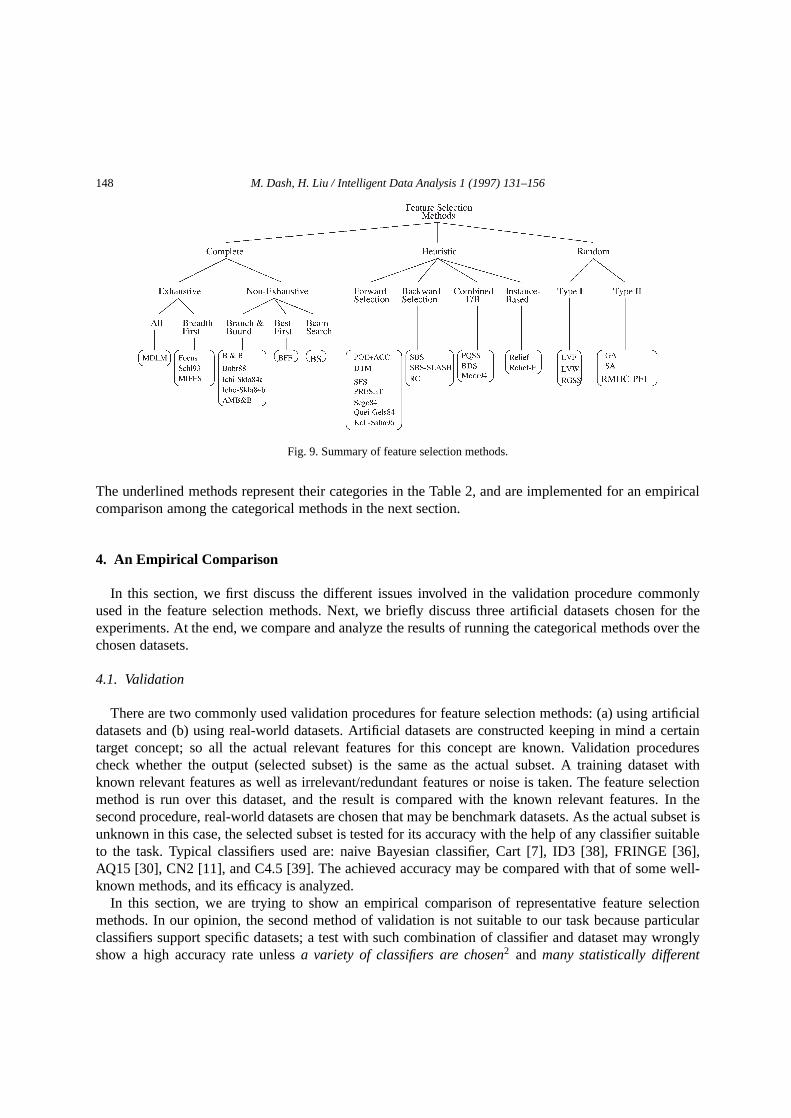
Figure 9 shows a summary of the feature selection methods based on the 3 types of generationprocedures. Complete generation procedures are further subdivided into ‘exhaustive’ and ‘non-exhaustive’; under ‘exhaustive’ category, a method may evaluate ‘All’ 2N subsets, or it may do a ‘breadth-first’ search to stop searching as soon as an optimal subset is found: under ‘non-exhaustive’ category wefind ‘branch & bound’, ‘best first’, and ‘beam search’ as different search techniques. Heuristic generationprocedures are subdivided into ‘forward selection’, ‘backward selection’, ‘combined forward/backward’,and ‘instance-based’ categories. Similarly, random generation procedures are grouped into ‘type I’ and‘type II.’ In ‘type I’ methods the probability of a subset to be generated remains constant, and it isthe same for all subsets, whereas in ‘type II’ methods this probability changes as the program runs.
148 M. Dash, H. Liu / Intelligent Data Analysis 1 (1997) 131–156
Fig. 9. Summary of feature selection methods.
The underlined methods represent their categories in the Table 2, and are implemented for an empiricalcomparison among the categorical methods in the next section.
4. An Empirical Comparison
In this section, we first discuss the different issues involved in the validation procedure commonlyused in the feature selection methods. Next, we briefly discuss three artificial datasets chosen for theexperiments. At the end, we compare and analyze the results of running the categorical methods over thechosen datasets.
4.1. Validation
There are two commonly used validation procedures for feature selection methods: (a) using artificialdatasets and (b) using real-world datasets. Artificial datasets are constructed keeping in mind a certaintarget concept; so all the actual relevant features for this concept are known. Validation procedurescheck whether the output (selected subset) is the same as the actual subset. A training dataset withknown relevant features as well as irrelevant/redundant features or noise is taken. The feature selectionmethod is run over this dataset, and the result is compared with the known relevant features. In thesecond procedure, real-world datasets are chosen that may be benchmark datasets. As the actual subset isunknown in this case, the selected subset is tested for its accuracy with the help of any classifier suitableto the task. Typical classifiers used are: naive Bayesian classifier, Cart [7], ID3 [38], FRINGE [36],AQ15 [30], CN2 [11], and C4.5 [39]. The achieved accuracy may be compared with that of some well-known methods, and its efficacy is analyzed.
In this section, we are trying to show an empirical comparison of representative feature selectionmethods. In our opinion, the second method of validation is not suitable to our task because particularclassifiers support specific datasets; a test with such combination of classifier and dataset may wronglyshow a high accuracy rate unlessa variety of classifiers are chosen2 and many statistically different

M. Dash, H. Liu / Intelligent Data Analysis 1 (1997) 131–156 149
datasets are used3. Also, as different feature selection methods have a different bias in selecting features,similar to that of different classifiers, it is not fair to use certain combinations of methods and classifiers,and try to generalize from the results that some feature selection methods are better than others withoutconsidering the classifier. Fortunately many recent papers, that introduce new feature selection methods,have done some extensive tests in comparison. Hence, if a reader wants to probe further, he/she is referredin this survey to the original work. To give some intuition regarding the wrapper methods, we includeone wrapper method (LVW [27]) in the empirical comparison along with the representative methods inthe categories I, II, IV, V, VII, XI, and XII (other categories are empty).
We choose three artificial datasets with combinations of relevant, irrelevant, redundant features, andnoise to perform comparison. They are simple enough but have characteristics that can be used for testing.For each dataset, a training set commonly used in literature for comparing the results, is chosen forchecking whether a feature selection method can find the relevant features.
4.2. Datasets
The three datasets are chosen in which the first dataset hasirrelevant and correlatedfeatures, thesecond hasirrelevant and redundantfeatures, and the third hasirrelevant features and it isnoisy(misclassification). Our attempt is to find out the strengths and weaknesses of the methods in thesesettings.
4.2.1. CorrAL[21]This dataset has 32 instances, binary classes, and six boolean features(A0,A1,B0,B1, I,C) out of
which featureI is irrelevant, featureC is correlatedto the class label 75% of the time, and the other fourfeatures are relevant to the boolean target concept:(A0\QA1)∼ (B0\QB1).
4.2.2. Modified Par3+3Par3+3 is a modified version of the original Parity3 data that has no redundant feature. The dataset
contains binary classes and twelve boolean features of which three features(A1,A2,A3) are relevant,(A7,A8,A9) are redundant, and(A4,A5,A6) and (A7,A8,A9) are irrelevant (randomly chosen). Thetraining set contains 64 instances and the target concept is the odd parity of the first three features.
4.2.3. Monk3[48]It has binary classes and six discrete features(A1, . . . ,A6) only the second, fourth and fifth of which
are relevant to the target concept:(A553∼A451)\Q(A5!54∼A2!53) with “!5” denoting inequality. Thetraining set contains 122 instances, 5% of which isnoise(misclassification).
4.3. Results and Analyses
Table 4 shows the results of running the eight categorical methods over the three artificial datasets. Inthe following paragraphs we analyze these results, and compare the methods based on the datasets used.
4.3.1. Relief[22]For CorrAL dataset, Relief selects(A0,B0,B1,C) for the range [14] ofNoSample.For all values of
NoSample, Relief prefers the correlated featureC over the relevant featureA1. The experiment over
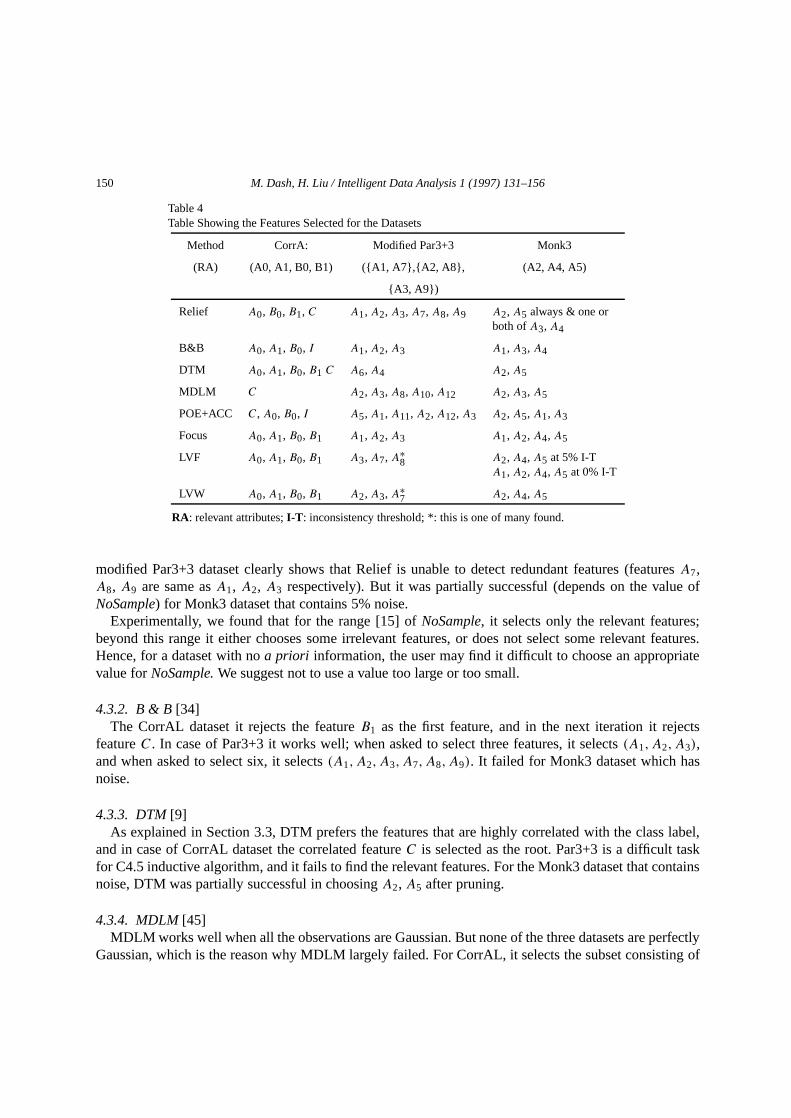
150 M. Dash, H. Liu / Intelligent Data Analysis 1 (1997) 131–156
Table 4Table Showing the Features Selected for the Datasets
Method CorrA: Modified Par3+3 Monk3
(RA) (A0, A1, B0, B1) ({A1, A7},{A2, A8}, (A2, A4, A5)
{A3, A9})
Relief A0, B0, B1, C A1,A2, A3,A7, A8,A9 A2,A5 always & one orboth ofA3,A4
B&B A0,A1, B0, I A1,A2, A3 A1,A3, A4
DTM A0,A1, B0, B1 C A6,A4 A2,A5
MDLM C A2,A3, A8,A10,A12 A2,A3, A5
POE+ACC C, A0, B0, I A5,A1, A11, A2,A12, A3 A2,A5, A1,A3
Focus A0,A1, B0, B1 A1,A2, A3 A1,A2, A4,A5
LVF A0,A1, B0, B1 A3,A7, A∗8 A2,A4, A5 at 5% I-TA1,A2, A4,A5 at 0% I-T
LVW A0,A1, B0, B1 A2,A3, A∗7 A2,A4, A5
RA: relevant attributes;I-T : inconsistency threshold; *: this is one of many found.
modified Par3+3 dataset clearly shows that Relief is unable to detect redundant features (featuresA7,A8, A9 are same asA1, A2, A3 respectively). But it was partially successful (depends on the value ofNoSample) for Monk3 dataset that contains 5% noise.
Experimentally, we found that for the range [15] ofNoSample, it selects only the relevant features;beyond this range it either chooses some irrelevant features, or does not select some relevant features.Hence, for a dataset with noa priori information, the user may find it difficult to choose an appropriatevalue forNoSample.We suggest not to use a value too large or too small.
4.3.2. B & B[34]The CorrAL dataset it rejects the featureB1 as the first feature, and in the next iteration it rejects
featureC. In case of Par3+3 it works well; when asked to select three features, it selects(A1,A2,A3),and when asked to select six, it selects(A1,A2,A3,A7,A8,A9). It failed for Monk3 dataset which hasnoise.
4.3.3. DTM[9]As explained in Section 3.3, DTM prefers the features that are highly correlated with the class label,
and in case of CorrAL dataset the correlated featureC is selected as the root. Par3+3 is a difficult taskfor C4.5 inductive algorithm, and it fails to find the relevant features. For the Monk3 dataset that containsnoise, DTM was partially successful in choosingA2, A5 after pruning.
4.3.4. MDLM[45]MDLM works well when all the observations are Gaussian. But none of the three datasets are perfectly
Gaussian, which is the reason why MDLM largely failed. For CorrAL, it selects the subset consisting of

M. Dash, H. Liu / Intelligent Data Analysis 1 (1997) 131–156 151
only the correlated featureC which indicates that it prefers correlated features. For the other two datasetsthe results are also not good.
4.3.5. POE+ACC[33]The results for this method show the rankings of the features. As seen, it was not very successful for any
of the dataset. For CorrAL, it chooses featureC as the first feature, as explained in Section 3.5. When wemanually input some other first features (e.g.,A0), then it correctly ranks the other three relevant featuresin the top four positions(A0,A1,B0,B1). This interesting finding points out the importance of the firstfeature on all the remaining features for POE+ACC. For Par3+3 and Monk3 it does not work well.
4.3.6. Focus[2]Focus works well when the dataset has no noise (as in the case of CorrAL and Par3+3), but it selects
an extra featureA1 for Monk3 that has 5% noise, as the actual subset(A2,A4,A5) does not satisfy thedefault inconsistency rate zero. Focus is also very fast in producing the results for CorrAL and Par3+3,because the actual subsets appear in the beginning which supports breadth-first search.
4.3.7. LVF[28]LVF works well for all the datasets in our experiment. For CorrAL it correctly selects the actual subset.
It is particularly efficient for Par3+3 that has three redundant features, because it can generate at leastone result out of the eight possible actual subsets quite early while randomly generating the subsets. Forthe Monk3 dataset, it needs an approximate noise level to produce the actual subset; otherwise (defaultcase of zero inconsistency rate) it selects an extra featureA1.
5. Discussions and Guidelines
Feature selection is used in many application areas as a tool to remove irrelevant and/or redundantfeatures. As is well known, there is no single feature selection method that can be applied to allapplications. The choice of a feature selection method depends on various data set characteristics: (i) datatypes, (ii) data size, and (iii) noise. Based on different criteria from these characteristics, we give someguidelines to a potential user of feature selection as to which method to select for a particular application.
5.1. Data Types
Various data types are found, in practice, forfeaturesandclass labels.Features: Feature values can be continuous (C), discrete (D), or nominal including boolean (N). The
nominal data type requires special handling because it is not easy to assign real values to it. Hence wepartition the methods based on theirability to handle different data types(C,D, N ).
Class Label: Some feature selection methods can handle only binary classes, and others can deal withmultiple (more than two) classes. Hence, the methods are separated based on theirability to handlemultiple classes.
152 M. Dash, H. Liu / Intelligent Data Analysis 1 (1997) 131–156
5.2. Data Size
This aspect of feature selection deals with: (i) whether a method can perform well for small trainingset, and (ii) whether it can handle large data size. In this information age, datasets are commonly largein size; hence the second criterion is more practical and of interest to the current as well as the futureresearchers and practitioners in this area [28]; so we separate the methods based on theirability to handlelarge dataset.
5.3. Noise
Typical noise encountered during the feature selection process are: (i) misclassification, and(ii) conflicting date ([29,41]). We partition the methods based on theirability to handle noise.
5.4. Some Guidelines
In this subsection we give some guidelines based on the criteria extracted from these characteristics.The criteria are as follows:
• ability to handle different data types (C: (Y/N), D: (Y/N), N: (Y/N)), where C, D, and N denotecontinuous, discrete, and nominal;• ability to handle multiple (more than two) classes (Y/N);• ability to handle large dataset (Y/N);• ability to handle noise (Y/N); and• ability to produce optimal subset if data is not noisy (Y/N).
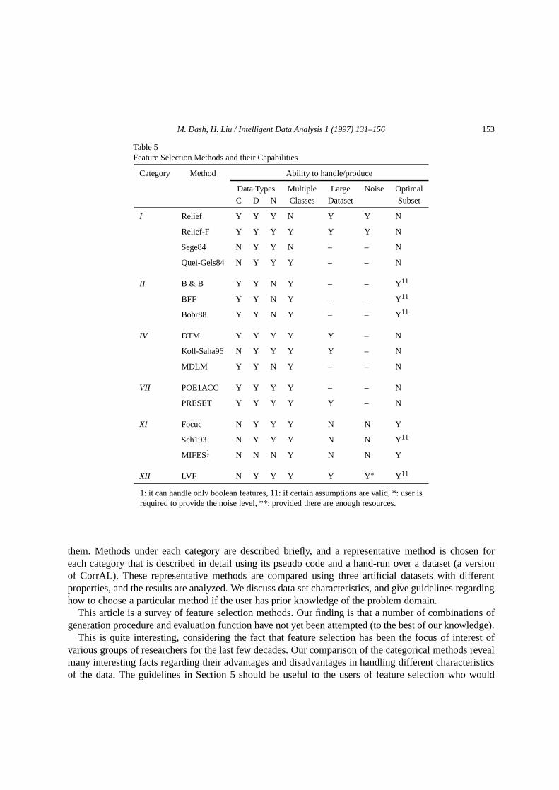
Table 5 lists the capabilities regarding these five characteristics of sixteen feature selection methods thatappear in the framework in Section 2. The methods having “classifier error rate” as an evaluation functionare not considered because their capabilities depend on the particular classifier used. A method can beimplemented in different ways, so the entries in the table are based on the presentation of the methods inthe papers. The “2” suggests that the method does not discuss the particular characteristics. A user mayemploy his/her prior knowledge regarding these five characteristics to find an appropriate method for aparticular application. For example, if the data contains noise, then the methods marked “Y” under thecolumn “Noise” should be considered. If there are more than one method satisfying the criteria mentionedby the user, then the user needs to have a closer look at the methods to find the most suitable among them,or design a new method that suits the application.
6. Conclusion and Further Work
We present a definition of feature selection after discussing many existing definitions. Four stepsof a typical feature selection process are recognized: generation procedure, evaluation function,stopping criterion, and validation procedure. We group the generation procedures into thee categories:complete, heuristic, and random, and the evaluation functions into five categories: distance, information,dependence, consistency, and classifier error rate measures. Thirty two existing feature selection methodsare categorized based on the combinations of generation procedure and evaluation function used in
M. Dash, H. Liu / Intelligent Data Analysis 1 (1997) 131–156 153
Table 5Feature Selection Methods and their Capabilities
Category Method Ability to handle/produce
Data Types Multiple Large Noise OptimalC D N Classes Dataset Subset
I Relief Y Y Y N Y Y N
Relief-F Y Y Y Y Y Y N
Sege84 N Y Y N – – N
Quei-Gels84 N Y Y Y – – N
II B & B Y Y N Y – – Y 11
BFF Y Y N Y – – Y11
Bobr88 Y Y N Y – – Y11
IV DTM Y Y Y Y Y – N
Koll-Saha96 N Y Y Y Y – N
MDLM Y Y N Y – – N
VII POE1ACC Y Y Y Y – – N
PRESET Y Y Y Y Y – N
XI Focuc N Y Y Y N N Y
Sch193 N Y Y Y N N Y11
MIFES11 N N N Y N N Y
XII LVF N Y Y Y Y Y ∗ Y11
1: it can handle only boolean features, 11: if certain assumptions are valid, *: user isrequired to provide the noise level, **: provided there are enough resources.
them. Methods under each category are described briefly, and a representative method is chosen foreach category that is described in detail using its pseudo code and a hand-run over a dataset (a versionof CorrAL). These representative methods are compared using three artificial datasets with differentproperties, and the results are analyzed. We discuss data set characteristics, and give guidelines regardinghow to choose a particular method if the user has prior knowledge of the problem domain.
This article is a survey of feature selection methods. Our finding is that a number of combinations ofgeneration procedure and evaluation function have not yet been attempted (to the best of our knowledge).
This is quite interesting, considering the fact that feature selection has been the focus of interest ofvarious groups of researchers for the last few decades. Our comparison of the categorical methods revealmany interesting facts regarding their advantages and disadvantages in handling different characteristicsof the data. The guidelines in Section 5 should be useful to the users of feature selection who would
154 M. Dash, H. Liu / Intelligent Data Analysis 1 (1997) 131–156
have been otherwise baffled by the sheer number of methods. Properly used, these guidelines can be ofpractical value in choosing the suitable method.
Although feature selection is a well-developed research area, researchers still try to find better methodsto make their classifiers more efficient. In this scenario the framework which shows the unattemptedcombinations of generation procedures and evaluation functions will be helpful. By testing particularimplementation of evaluation function and generation procedure combinations previously used in somecategories, we can design new and efficient methods for some unattempted combinations. It is obviousthat not all combinations will be efficient. The combination of consistency measure and heuristicgeneration procedure in the category ‘X’ may give some good results. One may also test differentcombinations that previously exist, such as branch and bound generation procedure and consistencymeasure in category XI.
Acknowledgments
The authors wish to thank the two referees, and Professor Hiroshi Motoda of Osaka University for theirvaluable comments, constructive suggestion, and thorough reviews on the earlier version of this article.Thanks also to Lee Leslie Leon, Sng Woei Tyng, and Wong Siew Kuen for implementing some of thefeature selection methods and analyzing their results.
References
[1] Aha, D.W., Kibler, D. and Albert, M.K.,Instance-Based Learning Algorithms. Machine Learning, 6:37–66, 1991.[2] Almuallim, H., and Dietterich, T.G., Learning with many irrelevant features. In:Proceedings of Ninth National Conference
on Artifical Intelligence, MIT Press, Cambridge, Massachusetts, 547–552, 1992.[3] Almuallim, H., and Dietterich, T.G.,Learning Boolean Concepts in the Presence of Many Irrelevant Features. Artificial
Intelligence, 69(1–2):279–305, November, 1994.[4] Ben-Bassat, M., Pattern recognition and reduction of dimensionality. In:Handbook of Statistics, (P. R. Krishnaiah and
L. N. Kanal, eds.), North Holland, 773–791, 1982.[5] Bobrowski, L., Feature selection based on some homogeneity coefficient. In:Proceedings of Ninth International
Conference on Pattern Recognition, 544–546, 1988.[6] Brassard, G., and Bratley, P.,Fundamentals of Algorithms. Prentice Hall, New Jersey, 1996.[7] Breiman, G., Friedman, J.H., Olshen, R.A. and Stone, C.J.,Classification and Regression Trees. Wadsworth International
Group, Belmont, California, 1984.[8] Callan, J.P., Fawcett, T.E. and Rissland, E.L., An adaptive approach to case-based search. In:Proceedings of the Twelfth
International Joint Conference on Artificial Intelligence, 803–808, 1991.[9] Cardie, C., Using decision trees to improve case-based learning. In:Proceedings of Tenth International Conference on
Machine Learning, 25–32, 1993.[10] Caruana, R. and Freitag, D., Greedy attribute selection. In:Proceedings of Eleventh International Conference on Machine
Learning, Morgan Kaufmann, New Brunswick, New Jersey, 28–36, 1994.[11] Clark, P. and Niblett, T., The CN2 Induction Algorithm.Machine Learning, 3:261–283, 1989.[12] Devijver, P.A. and Kittler, J.,Pattern Recognition: A Statistical Approach. Prentice Hall, 1982.[13] Doak, J.,An evaluation of feature selection methods and their application to computer security. Technical report, Davis,
CA: University of California, Department of Computer Science, 1992.[14] Domingos, P., Context-sensitive feature selection for lazy learners.Artificial Intelligence Review, 1996.[15] Duran, B.S. and Odell, P.K.,Cluster Analysis—A Survey. Springer-Verlag, 1974.[16] Foroutan, I. and Sklansky, J., Feature selection for automatic classification of non-gaussian data.IEEE Transactions on
Systems, Man, and Cybernatics, SMC-17(2):187–198, 1987.
M. Dash, H. Liu / Intelligent Data Analysis 1 (1997) 131–156 155
[17] Geoffrion, A.M., Integer programming by implicit enumeration and balas, method.SIAM Review, 9:178–190, 1967.[18] Holte, R.C., Very simple classification rules perform well on most commonly used datasets.Machine Learning, 11(1):63–
90, 1993.[19] Ichino, M. and Sklansky, J., Feature selection for linear classifier. In:Proceedings of the Seventh International Conference
on Pattern Recognition, volume 1, 124–127, July–Aug 1984.[20] Ichino, M. and Sklansky, J., Optimum feature selection by zero-one programming.IEEE Trans. on Systems, Man and
Cybernetics, SMC-14(5):737–746, September/October 1984.[21] John, G.H., Kohavi, R. and Pfleger, K., Irrelevant features and the subset selection problem. In:Proceedings of the Eleventh
International Conference on Machine Learning, 121–129, 1994.[22] Kira, K. and Rendell, L.A., The feature selection problem: Traditional methods and a new algorithm. In:Proceedings of
Ninth National Conference on Artificial Intelligence, 129–134, 1992.[23] Kohavi, R. and Sommerfield, D., Feature subset selection using the wrapper method: Overfitting and dynamic search
space topology. In:Proceedings of First International Conference on Knowledge Discovery and Data Mining, MorganKaufmann, 192–197, 1995.
[24] Koller, D. and Sahami, M., Toward optimal feature selection. In:Proceedings of International Conference on MachineLearning, 1996.
[25] Kononenko, I., Estimating attributes: Analysis and extension of RELIEF. In:Proceedings of European Conference onMachine Learning, 171–182, 1994.
[26] Langley, P., Selection of relevant features in machine learning. In:Proceedings of the AAAI Fall Symposium on Relevance,1–5, 1994.
[27] Liu, H. and Setiono, R., Feature selection and classification—a probabilistic wrapper approach. In:Proceedings of NinthInternational Conference on Industrial and Engineering Applications of AI and ES, 284–292, 1996.
[28] Liu, H. and Setiono, R., A probabilistic approach to feature selection—a filter solution. In:Proceedings of InternationalConference on Machine Learning, 319–327, 1996.
[29] Michalski, R.S., Carbonell, J.G. and Mitchell, T.M (eds.), The effect of noise on concept learning, In:Machine Learning:An Artificial Intelligence Approach(vol. II), Morgan Kaufmann, San Mateo, CA, 419–424, 1986.
[30] Michalski, R.S., Mozetic, I., Hong, J. and Lavrac, N., The aq15 inductive learning system: An overview and experiments.Technical Report UIUCDCS-R-86-1260, University of Illinois, July 1986.
[31] Modrzejewski, M., Feature selection using rough sets theory. In:Proceedings of the European Conference on MachineLearning(P. B. Brazdil, ed.), 213–226, 1993.
[32] Moore, A.W. and Lee, M.S., Efficient algorithms for minimizing cross validation error. In:Proceedings of EleventhInternational Conference on Machine Learning, Morgan Kaufmann, New Brunswick, New Jersey, 190–198, 1994.
[33] Mucciardi, A.N. and Gose, E.E., A comparison of seven techniques for choosing subsets of pattern recognition.IEEETransactions on Computers, C-20:1023–1031, September 1971.
[34] Narendra, P.M. and Fukunaga, K., A branch and bound algorithm for feature selection.IEEE Transactions on Computers,C-26(9):917–922, September 1977.
[35] Oliveira, A.L. and Vincentelli, A.S., Constructive induction using a non-greedy strategy for feature selection. In:Proceedings of Ninth International Conference on Machine Learning, 355–360, Morgan Kaufmann, Aberdeen, Scotland,1992.
[36] Pagallo, G. and Haussler, D., Boolean feature discovery in empirical learning.Machine Learning, 1(1):81–106, 1986.[37] Queiros, C.E. and Gelsema, E.S., On feature selection. In:Proceedings of Seventh International Conference on Pattern
Recognition, 1:128–130, July-Aug 1984.[38] Quinlan, J., Induction of decision trees. In:Machine Learning, Morgan Kaufmann, 81–106. 1986.[39] Quinlan, J.R., C4.5: Programs for Machine Learning. Morgan Kaufmann, San Mateo, California, 1993.[40] Rissanen, J., Modelling by shortest data description.Automatica, 14:465–471, 1978.[41] Schaffer, C., Overfitting avoidance as bias.Machine Learning, 10(2):153–178, 1993.[42] Schaffer, C., A conservation law for generalization performance. In:Proceedings of Eleventh International Conference on
Machine Learning, Morgan Kaufmann, New Brunswick, NJ, 259–265, 1994.[43] Schlimmer, J.C., Efficiently inducing determinations: A complete and systematic search algorithm that uses optimal
pruning. In:Proceedings of Tenth International Conference on Machine Learning, 284–290, (1993).[44] Segen, J., Feature selection and constructive inference. In:Proceedings of Seventh International Conference on Pattern
Recognition, 1344–1346, 1984.

156 M. Dash, H. Liu / Intelligent Data Analysis 1 (1997) 131–156
[45] Sheinvald, J., Dom, B. and Niblack, W., A modelling approach to feature selection. In:Proceedings of Tenth InternationalConference on Pattern Recognition, 1:535–539, June 1990.
[46] Siedlecki, W. and Sklansky, J., On automatic feature selection.International Journal of Pattern Recognition and ArtificialIntelligence, 2:197–220, 1988.
[47] Skalak, D.B., Prototype and feature selection by sampling and random mutation hill-climbing algorithms. In:Proceedingsof Eleventh International Conference on Machine Learning, Morgan Kaufmann, New Brunswick, 293–301, 1994.
[48] Thrun, S.B., et al., The monk’s problem: A performance comparison of different algorithms. Technical Report CMU-CS-91-197, Carnegie Mellon University, December 1991.
[49] Vafaie, H. and Imam, I.F., Feature selection methods: genetic algorithms vs. greedy-like search. In:Proceedings ofInternational Conference on Fuzzy and Intelligent Control Systems, 1994.
[50] Xu, L., Yan, P. and Chang, T., Best first strategy for feature selection. In:Proceedings of Ninth International Conferenceon Pattern Recognition, 706–708, 1988.
Related Documents


![Data Mining - [2] Classification - 07 - Feature Selection](https://static.cupdf.com/doc/110x72/61a90a7cc6cb190dbd05c382/data-mining-2-classification-07-feature-selection.jpg)