FC4: Fully Convolutional Color Constancy With Confidence ...openaccess.thecvf.com/content_cvpr_2017/papers/Hu...FC4: Fully Convolutional Color Constancy with Condence-weighted Pooling

FC4: Fully Convolutional Color Constancy with Confidence-weighted Pooling

Yuanming Hu1∗ Baoyuan Wang2 Stephen Lin2

1Tsinghua University, 2Microsoft Research

[email protected], {baoyuanw,stevelin}@microsoft.com

Abstract

Improvements in color constancy have arisen from the

use of convolutional neural networks (CNNs). However, the

patch-based CNNs that exist for this problem are faced with

the issue of estimation ambiguity, where a patch may con-

tain insufficient information to establish a unique or even a

limited possible range of illumination colors. Image patch-

es with estimation ambiguity not only appear with great fre-

quency in photographs, but also significantly degrade the

quality of network training and inference. To overcome

this problem, we present a fully convolutional network ar-

chitecture in which patches throughout an image can car-

ry different confidence weights according to the value they

provide for color constancy estimation. These confidence

weights are learned and applied within a novel pooling lay-

er where the local estimates are merged into a global so-

lution. With this formulation, the network is able to de-

termine “what to learn” and “how to pool” automatical-

ly from color constancy datasets without additional super-

vision. The proposed network also allows for end-to-end

training, and achieves higher efficiency and accuracy. On s-

tandard benchmarks, our network outperforms the previous

state-of-the-art while achieving 120× greater efficiency.

1. Introduction

Computational color constancy is a longstanding prob-

lem, where the goal is to remove illumination color casts

in images. This form of color correction can benefit down-

stream applications such as visual recognition, where color

is an important feature for distinguishing objects. Despite

various needs for accurate color constancy, there remains

much room for improvement among current algorithms due

to the significant challenges that this task presents.

State-of-the-art techniques [38, 6, 7, 31, 5] have har-

nessed the power of convolutional neural networks (CNNs)

to learn color constancy models from large training sets,

∗This work was done when Yuanming Hu was an intern at Microsoft

Research.

Computational Color Constancy

ground truth illumination estimation

estimation error

Input Output (color cast removed)

both plausible,but which one

is correct?

Example Image

Ambiguous

Informative

ReflectanceIllumination ×= ×××=

=

=

Patch

= ... lots of other combinations

Reflectance is probably yellow

white illum.

restricted possible reflectance higher illum. est. confidence

yellow light

yellow wall

white wall

white light

white light

yellow light

yellow banana

white banana (does not exist)

Confidence mapInput Robust Outputillum. est. (noisy)

weighted illum. est.

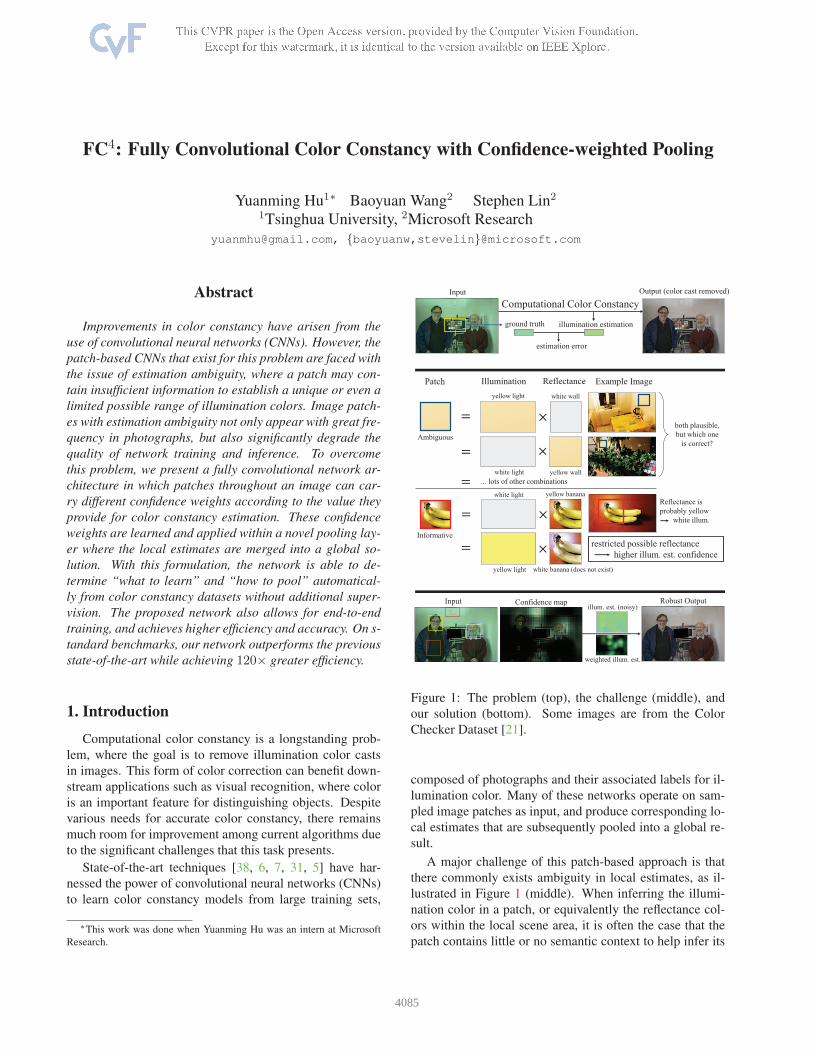
Figure 1: The problem (top), the challenge (middle), and

our solution (bottom). Some images are from the Color

Checker Dataset [21].

composed of photographs and their associated labels for il-

lumination color. Many of these networks operate on sam-

pled image patches as input, and produce corresponding lo-

cal estimates that are subsequently pooled into a global re-

sult.

A major challenge of this patch-based approach is that

there commonly exists ambiguity in local estimates, as il-

lustrated in Figure 1 (middle). When inferring the illumi-

nation color in a patch, or equivalently the reflectance col-

ors within the local scene area, it is often the case that the

patch contains little or no semantic context to help infer its

4085

reflectance or illumination. If the classes of objects with-

in a patch can be of arbitrary reflectance (such as a painted

wall), then there may be a broad range of illuminations that

can plausibly explain the patch’s appearance in an image.

On the other hand, patches containing objects that have an

innate color (such as bananas) provide cues that are much

more informative for color constancy estimation. In patch-

based CNNs, these two types of patches are treated equally,

even though patches that are ambiguous for color constan-

cy provide little or no value, and furthermore inject noise

into both CNN training and inference. Noisy data adverse-

ly affects CNN-based estimation, as noted in recent works

on object recognition [34] and image classification [41, 43].

For color constancy, noise is an especially concerning issue,

since ambiguous patches occur at high frequency within

many photographs and may diminish the influence of more

valuable patches.

To address this problem, we propose a fully convolution-

al network, called FC4, where the patches in an input image

can differ in influence over the color constancy estimation.

This influence is formulated as a confidence weight that re-

flects the value of a patch for inferring the illumination col-

or. The confidence weights are integrated into a novel pool-

ing layer where they are applied to local patch estimates in

determining a global color constancy result. In contrast to

existing patch-based CNNs for this problem, which process

patches sequentially and individually, FC4 considers all of

the image patches together at the same time, which allows

the usefulness of patches to be compared and learned dur-

ing training. In this way, the network can learn from color

constancy datasets about which local areas in an image are

informative for color constancy and how to combine their

information to produce a final estimation result.

This network design with joint patch processing and

confidence-weighted pooling not only distinguishes be-

tween useful and noisy data in both the training and eval-

uation phases, but also confers other advantages including

end-to-end training, direct processing of images with arbi-

trary size, and much faster computation. Our experiments

show that FC4 compares favorably in performance to state-

of-the-art techniques, and is also less prone to large esti-

mation errors. Aside from its utility for color constancy,

the proposed scheme for learning and pooling confidence

weights may moreover be useful for other vision problems

in which a global estimate is determined from aggregated

local inferences.

2. Related Work

Color constancy Methods for computational color con-

stancy fall mainly into two categories: statistics-based and

learning-based. The former assumes certain statistical prop-

erties of natural scenes, such as an average surface re-

flectance of gray [11], and solves for an illumination color

that explains the deviation of an image from that property.

A unified model for various statistics-based methods was

presented by Van De Weijer et al. [42].

Learning-based techniques estimate illumination color

using a model learned from training data. This approach has

become prevalent because of its generally higher accuracy

relative to statistics-based methods. Many of these tech-

niques employ models based on handcrafted features [12,

18, 20, 35, 15], while the most recent works learn features

using convolutional neural networks [6, 31, 5, 7, 38]. Here,

we will review these latter works, which yield the highest

performance and are the most relevant to ours. We refer

readers to the surveys in [24] and [23] for additional back-

ground.

Among the CNN-based approaches, there are those that

operate on local patches as input [38, 6, 7], while others

directly take full image data [5, 31]. In the work of Bar-

ron [5]1, the full image data is in the form of various chro-

ma histograms, for which convolutional filters are learned

to discriminatively evaluate possible illumination color so-

lutions in the chroma plane. As spatial information is on-

ly weakly encoded in these histograms, semantic context

is largely ignored. The method of Lou et al. [31] instead

uses the image itself as input. It thus considers semantic

information at a global level, where the significance of se-

mantically valuable local regions is difficult to discern. The

learning is further complicated by the limited number of full

images for color constancy training. Also, as their CNN is

not fully convolutional, test images need to be resized to

predefined dimensions, which may introduce spatial distor-

tions of image content. While our network also takes a full

image as input, it does not suffer from these limitations, as

its estimation is based on windows within the image, and

the network is formulated in a fully convolutional structure.

Patch-based CNNs were first used for color constancy by

Bianco et al., where a conventional convolutional network

is used to extract local features which are then pooled [6] or

passed to a support vector regressor [7] to estimate illumina-

tion color. Later, Shi et al. [38] proposed a more advanced

network to deal with estimation ambiguities, where multi-

ple illumination hypotheses are generated for each patch in

a two-branch structure, and a selection sub-network adap-

tively chooses an estimate from among the hypotheses. Our

work also employs a selection mechanism, but instead s-

elects which patches in an image are used for estimation.

Learning the semantic value of local regions makes our ap-

proach more robust to the estimation ambiguities addressed

in [38], as semantically ambiguous patches can then be pre-

vented from influencing the illumination estimation.

Related to patch-based CNNs is the method of Bianco

and Schettini [8, 9], which focuses specifically on face re-

1Though the system in [5] utilizes only a single convolutional layer, we

include it in our discussion of CNN-based methods.

4086

Patch-based Image-based Histograms Ours

[38, 6, 7] [31] [5]

Ample training data � × � �

Semantic info. � only global × �

End-to-end × � × �

Arbitrary-sized input � × � �

Noisy data masking × - - �

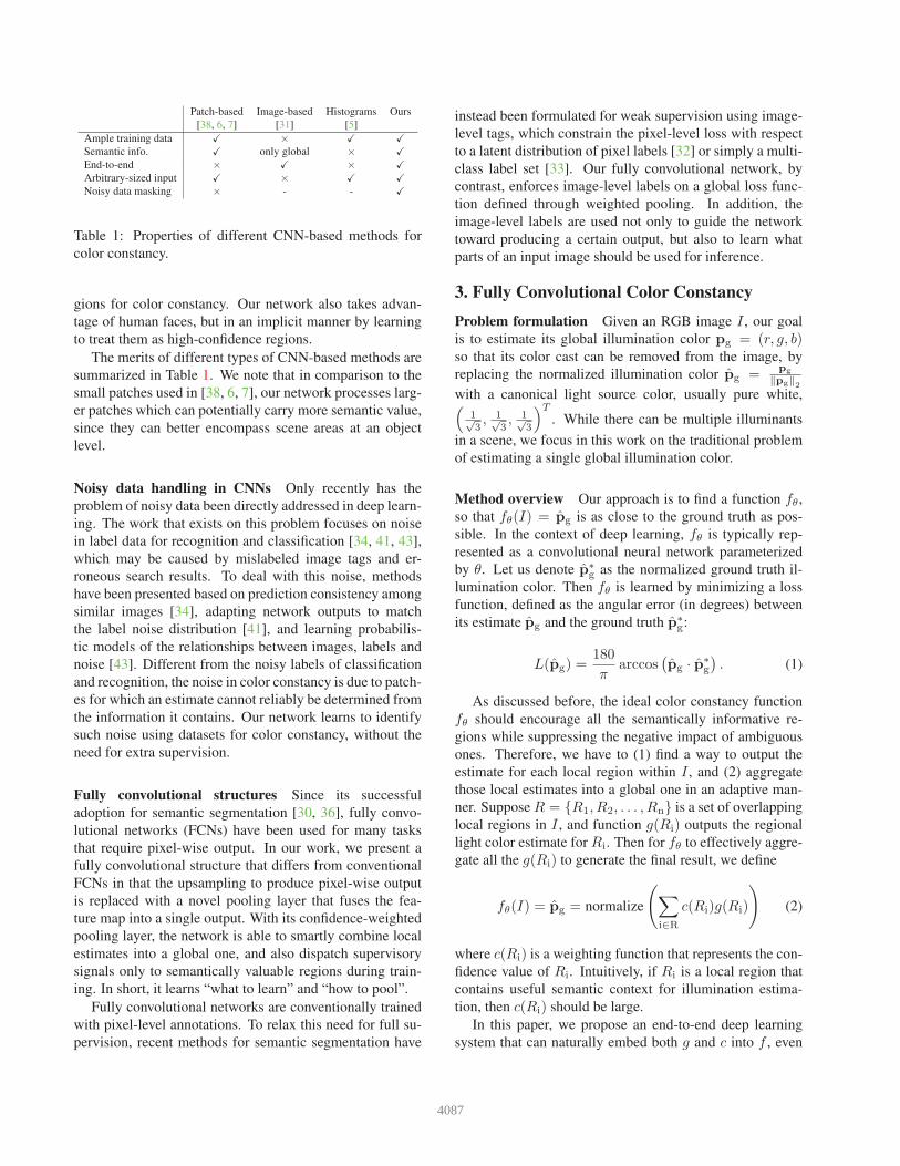
Table 1: Properties of different CNN-based methods for

color constancy.

gions for color constancy. Our network also takes advan-

tage of human faces, but in an implicit manner by learning

to treat them as high-confidence regions.

The merits of different types of CNN-based methods are

summarized in Table 1. We note that in comparison to the

small patches used in [38, 6, 7], our network processes larg-

er patches which can potentially carry more semantic value,

since they can better encompass scene areas at an object

level.

Noisy data handling in CNNs Only recently has the

problem of noisy data been directly addressed in deep learn-

ing. The work that exists on this problem focuses on noise

in label data for recognition and classification [34, 41, 43],

which may be caused by mislabeled image tags and er-

roneous search results. To deal with this noise, methods

have been presented based on prediction consistency among

similar images [34], adapting network outputs to match

the label noise distribution [41], and learning probabilis-

tic models of the relationships between images, labels and

noise [43]. Different from the noisy labels of classification

and recognition, the noise in color constancy is due to patch-

es for which an estimate cannot reliably be determined from

the information it contains. Our network learns to identify

such noise using datasets for color constancy, without the

need for extra supervision.

Fully convolutional structures Since its successful

adoption for semantic segmentation [30, 36], fully convo-

lutional networks (FCNs) have been used for many tasks

that require pixel-wise output. In our work, we present a

fully convolutional structure that differs from conventional

FCNs in that the upsampling to produce pixel-wise output

is replaced with a novel pooling layer that fuses the fea-

ture map into a single output. With its confidence-weighted

pooling layer, the network is able to smartly combine local

estimates into a global one, and also dispatch supervisory

signals only to semantically valuable regions during train-

ing. In short, it learns “what to learn” and “how to pool”.

Fully convolutional networks are conventionally trained

with pixel-level annotations. To relax this need for full su-

pervision, recent methods for semantic segmentation have

instead been formulated for weak supervision using image-

level tags, which constrain the pixel-level loss with respect

to a latent distribution of pixel labels [32] or simply a multi-

class label set [33]. Our fully convolutional network, by

contrast, enforces image-level labels on a global loss func-

tion defined through weighted pooling. In addition, the

image-level labels are used not only to guide the network

toward producing a certain output, but also to learn what

parts of an input image should be used for inference.

3. Fully Convolutional Color Constancy

Problem formulation Given an RGB image I , our goal

is to estimate its global illumination color pg = (r, g, b)so that its color cast can be removed from the image, by

replacing the normalized illumination color pg =pg

‖pg‖2

with a canonical light source color, usually pure white,(

1√3, 1√

3, 1√

3

)T

. While there can be multiple illuminants

in a scene, we focus in this work on the traditional problem

of estimating a single global illumination color.

Method overview Our approach is to find a function fθ,

so that fθ(I) = pg is as close to the ground truth as pos-

sible. In the context of deep learning, fθ is typically rep-

resented as a convolutional neural network parameterized

by θ. Let us denote p∗g as the normalized ground truth il-

lumination color. Then fθ is learned by minimizing a loss

function, defined as the angular error (in degrees) between

its estimate pg and the ground truth p∗g:

L(pg) =180

πarccos

(

pg · p∗g

)

. (1)

As discussed before, the ideal color constancy function

fθ should encourage all the semantically informative re-

gions while suppressing the negative impact of ambiguous

ones. Therefore, we have to (1) find a way to output the

estimate for each local region within I , and (2) aggregate

those local estimates into a global one in an adaptive man-

ner. Suppose R = {R1, R2, . . . , Rn} is a set of overlapping

local regions in I , and function g(Ri) outputs the regional

light color estimate for Ri. Then for fθ to effectively aggre-

gate all the g(Ri) to generate the final result, we define

fθ(I) = pg = normalize

(

∑

i∈R

c(Ri)g(Ri)

)

(2)

where c(Ri) is a weighting function that represents the con-

fidence value of Ri. Intuitively, if Ri is a local region that

contains useful semantic context for illumination estima-

tion, then c(Ri) should be large.

In this paper, we propose an end-to-end deep learning

system that can naturally embed both g and c into f , even

4087

× ℎ ×

input imageconv1-5

from AlexNet

conv/ReLU/max pooling layers

summation

max poolingconv6:6 × 6 × 6 conv7:× ×

=×

Confidence-weighted pooling

semi-densefeature maps

conv6, conv7 randomly initialized

× ℎ ×

× ℎ ×

× ℎ ×

FC4

normalizationillumination color

restored image

high confidence image regions

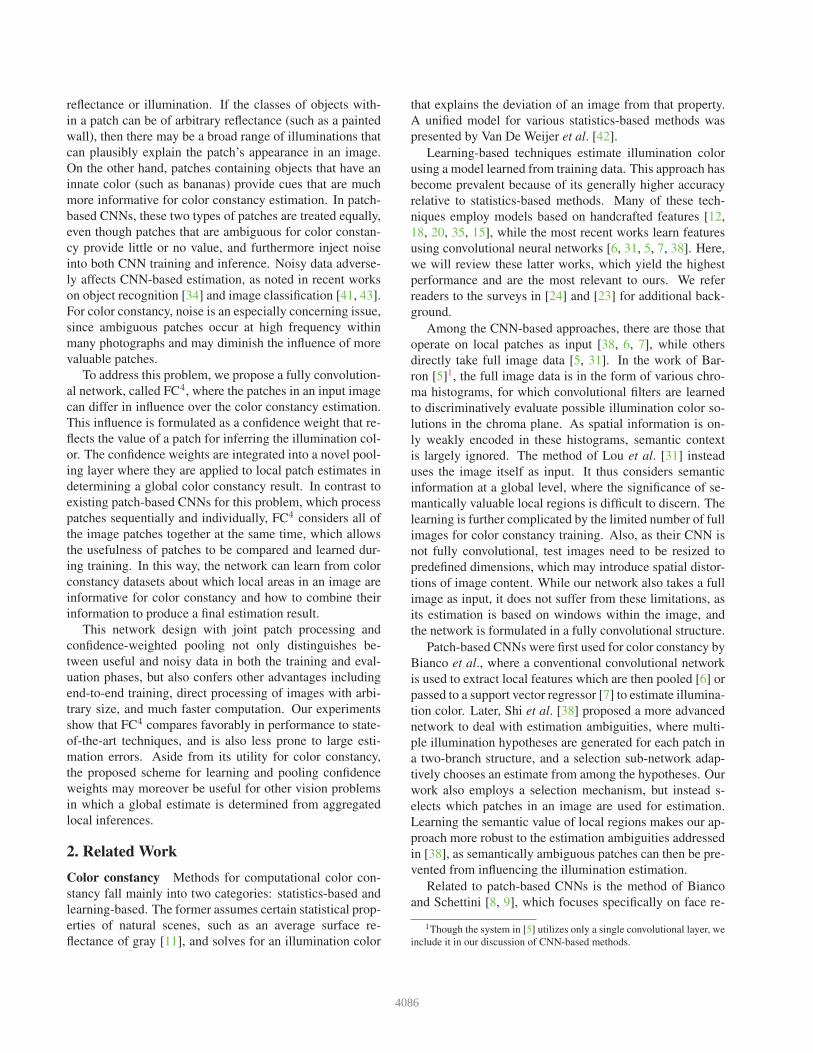
Figure 2: The architecture of AlexNet-FC4. Replacing AlexNet (conv1-conv5) with SqueezeNet v1.1 (conv1-fire8 plus an

extra 2× 2 pooling) yields SqueezeNet-FC4.

though we have no explicit supervision for either g or c. The

network should learn to fuse optimal combinations of local

estimates, through adaptive use of the corresponding g and

c for each local region such that the impact of ambiguous

patches will be suppressed. Toward this end, we propose

a novel architecture based on a fully convolutional network

(FCN) and a weighted pooling layer that are tailored for the

color constancy problem. Figure 2 shows the architecture

of our network.

3.1. Fully Convolutional Architecture

Following the observation that mid-level semantic infor-

mation provides more clues for illumination estimation, we

extract medium-sized window regions R = {Ri} from I as

square subsets of the image. For each region, the estimate

made by function g(Ri) is denoted as pi. Unlike previous

patch-based methods, such as [7], which treat each Ri in-

dependently over an image and use a CNN to learn g, we

instead consider all of the local patches within the same im-

age jointly so that their relative importance for estimating

the global illumination color can be well explored. There-

fore, given an image, we wish to determine the local es-

timates simultaneously. Fortunately, a fully convolutional

network can accomplish our goal by sharing all the convo-

lution computations in a natural way and predicting all the

spatially local estimates at the same time. In addition, an

FCN can take an input of any size, which avoids distortions

of semantic information that may occur with CNN methods

that employ resizing [31].

We design our fully convolutional network as shown in

Figure 2. As our basic model for extracting semantic fea-

tures for each patch, we adapt all the layers up to conv5 of

AlexNet [29], which are pretrained on ImageNet [16]. A

relatively large conv6 (6 × 6 × 64) and subsequent conv7

(1× 1× 4 for dimensionality reduction) are further used in

extracting semi-dense feature maps. Those feature maps are

passed to a weighted pooling layer to aggregate from local

to global to generate the final color constancy estimate as

described in Eqn. 2.

Note that, within the four channels in the semi-dense

feature maps, we force the first three channels to represen-

t the color triplet pi = g(Ri) estimated from each corre-

sponding patch, while the last one represents its confidence

ci = c(Ri) in contributing to the final global estimation.

The four channels are passed through a ReLU layer to avoid

negative values, and the final estimated RGB channels are

l2-normalized per pixel. We define the weighted estimate

pi as cipi.

Discussion Theoretically, either shallower (i.e. [38]) or

deeper networks (i.e., VGG-16 [39] or [2]) could be used

to replace AlexNet in our system. However, due to the na-

ture of the color constancy problem, the best model is con-

strained by at least two important properties: (1) the net-

work should be able to extract sufficient semantic features to

discriminate ambiguous patches (such as textureless walls)

for illumination estimation, and (2) the network should not

be illumination invariant, but rather it should be sensitive to

different lighting colors. As we can see, the second require-

ment violates the knowledge embedded in networks trained

on classification tasks, since lighting conditions should not

affect the class of an object. Unfortunately, networks with

4088

strong ability to extract semantic information are usually al-

so insensitive to changing lighting conditions, meaning that

the extracted features are invariant to illumination color.

To find a good balance between the two aforementioned

properties, we experimented with different network config-

urations. We tried a shallower version of AlexNet with con-

v4 and/or conv5 removed, and found that the performance

becomes worse, perhaps due to insufficient ability for se-

mantic feature extraction. In addition, we tried other kernel

sizes for conv6, including 1×1, 3×3 and 10×10, but found

that 6 × 6, which is the original output size of AlexNet af-

ter the convolution layers, leads to the best results. To re-

duce model size, we experimented with SqueezeNet [25]

v1.1 and found that it also leads to good results.

3.2. Confidence-weighted Pooling Layer

As explained earlier, different local regions may differ

in value for illumination estimation based on their seman-

tic content. To treat these patches differently, a function

c(Ri) is regressed to output the confidence values of the

corresponding estimates. Although a function c could be

modeled as a separate fully convolutional branch originat-

ing from conv5 or even lower layers, it is more straightfor-

ward to implement it jointly as a fourth channel that is in-

cluded with the three color channels of each local illumina-

tion estimate. The final result is simply a weighted-average

pooling of all the local estimates, as expressed in Eqn. 3 and

4.

Note that patch based training with average pooling can

be regarded as a special case of our network by setting each

c(Ri) = 1. In our network, thanks to the FCN architecture,

convolutional operations are shared among patches with-

in the same image, while for the patch-based CNNs each

patch needs to go through the same network sequentially.

There also exist other pooling methods, such as fully con-

nected pooling or max-pooling; however, they either lack

flexibility (i.e., require a specific input image size) or have

been shown to be not very effective for color constancy es-

timation. Median pooling does a better job according to

[38], as it prevents outliers from contributing directly to the

global estimation, but it does not completely eliminate their

impact when a significant proportion of the estimates are

noisy. Furthermore, even if we incorporate it in an end-to-

end training pipeline, the loss can only back-propagate to a

single (median) patch in the image each time, ignoring pair-

wise dependencies among the patches. For a comparison of

different pooling methods, please refer to Table 2.

Mathematical analysis Here we show where the abili-

ty of learning the confidence comes from, by a more rigid

mathematical analysis. During back-propagation, this pool-

ing layer serves as a “gradient dispatcher” which back-

propagates gradients to local regions with respect to their

confidence. Let us take a closer look at the pooling layer

by differentiating the loss function with respect to a local

estimate pi and confidence c(Ri) (denoted as ci in the fol-

lowing for simplicity). The weighted pooling is defined as

pg =∑

i∈R

cipi, (3)

pg =pg

‖pg‖2=

1

‖pg‖2

∑

i∈R

cipi. (4)

Then by the chain rule, we get

∂L(pg)

∂pi

=ci

‖pg‖2·∂L(pg)

∂pg

. (5)

From the above, it can be seen that among the estimates pi,

their gradients all share the same direction but have differ-

ent magnitudes that are proportional to ci, the confidence.

So for the local estimates, the confidence serves as a mask

for the supervision signal, which prevents our network from

learning noisy data.

Similarly, for confidence ci, we have

∂L(pg)

∂ci=

1

‖pg‖2·∂L(pg)

∂pg

· pi. (6)

Intuitively, as long as a local estimate helps the global

estimation get closer to the ground truth, the network in-

creases the corresponding confidence. Otherwise, the con-

fidence will be reduced. This is exactly how the confidence

should be learned. Please refer to the supplementary ma-

terial for a more detailed deduction and illustration of the

training cycle.

4. Experimental Results

4.1. Settings

Implementation and Training Our network was imple-

mented in TensorFlow [1]. Explicitly outputting ci and pi

after conv7 is mathematically clearer, and in practice we

found that directly outputting the weighted estimate pi in-

stead, where ci and pi are implicitly the norm and direction

of pi, leads to similar accuracy and also a simpler imple-

mentation.

We trained our network end-to-end by back-propagation.

For optimization, Adam [28] is employed with a batch size

of 16 and a base learning rate of 1× 10−4 for AlexNet and

3 × 10−4 for SqueezeNet. We fine-tuned all of the con-

volutional layers from the pre-trained networks. Since the

color constancy task is quite different from the original im-

age classification task, we use the same learning rate for the

pre-trained layers as for the last two layers, instead of small-

er ones, to expedite their adaptation to color constancy. We

also include a dropout [40] probability of 0.5 for conv6 and

a weight decay of 5 × 10−5 for all layers to help prevent

overfitting.

4089

Data augmentation and preprocessing Considering the

relatively small size of color constancy datasets, we aug-

mented the data aggressively on-the-fly. To facilitate this

augmentation, we use square crops of the images, which are

initially obtained by first randomly choosing a side length

that is 0.1 ∼ 1 times the shorter edge of the original im-

age, and then randomly selecting the upper-left corner of

the square. The crop is rotated by a random angle between

−30◦ ∼ +30◦, and is left-right flipped with a probabil-

ity of 0.5. When training SqueezeNet-FC4 on [37], we

rescale images and ground truth by random RGB values in

[0.6, 1.4]. Finally, we resize the crop to 512px×512px and

feed a batch of them to the network for training. In testing,

the images are downsampled to 50% for faster processing.

Since AlexNet and SqueezeNet are pretrained on Ima-

geNet [16], where images are gamma-corrected for display,

we apply a gamma correction of γ = 1/2.2 on linear RGB

images to make them more similar to those in ImageNet.

Datasets Two standard datasets are used for benchmark-

ing: the reprocessed [37] Color Checker Dataset [21] and

the NUS 8-Camera Dataset [14]. These datasets contain

568 and 1736 raw images, respectively. In the NUS 8-

Camera Dataset, the images are divided into 8 subsets of

about 210 images for each camera. As a result, although

the total number of images is larger, each independent ex-

periment on the NUS 8-Camera Dataset involves only about

1/3 the number of images in the reprocessed Color Check-

er Dataset. For images in both datasets, a Macbeth Color

Checker (MCC) is present for obtaining the ground truth il-

lumination color. The corners of the MMCs are provided

by the datasets, and we mask the MCCs by setting the en-

closed image regions to RGB = (0, 0, 0) for both training

and testing. No other special processing was done for these

regions. Both datasets contain photos of different orienta-

tions, and the Color Checker Dataset has photos of different

sizes from two cameras. Our fully convolutional networks

naturally handle these arbitrary-sized inputs.

Following previous work, three-fold cross validation is

used for both datasets. Several standard metrics are reported

in terms of angular error in degrees: mean, median, tri-mean

of all the errors, mean of the lowest 25% of errors, and mean

of the highest 25% of errors. For the reprocessed Color

Checker Dataset, we additionally report the 95th percentile

error. For the NUS dataset, we also report the geometric

mean (G.M. in Table 5) of the other five metrics.

4.2. Internal comparisons

We compare FC4 with variants of itself that employ oth-

er combinations of pooling layers and network inputs. This

evaluation of accuracy and speed is performed on the repro-

cessed Color Checker Dataset, and the results are shown in

Table 3.

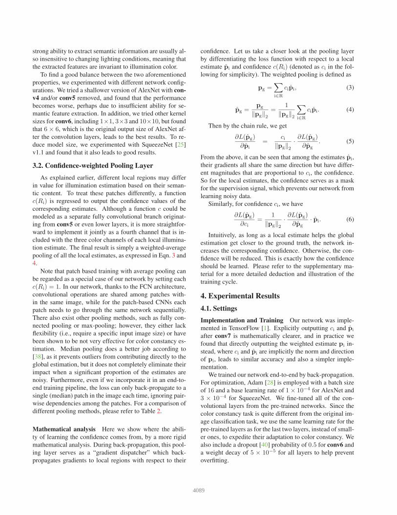
FC layer average median weighted

End-to-end training �� �� � ��Arbitrary-sized input � � �Noisy data masking � �� � � �Parameter-free � � �

Table 2: Comparison of different pooling methods. More

stars stands for stronger property.

Pooling layers To examine the improvements induced by

confidence-weighted pooling, we experimentally compare

it to the following alternatives:

• Fully connected (FC) layer, which takes the feature

map from the last convolutional layer as input, and out-

puts RGB values. This is very similar to traditional C-

NNs which are not fully convolutional. Note that one

drawback of FC layers is their fixed input size, which

requires rescaling or trimming of images. Because of

its learnable parameters, an FC layer introduces extra

network complexity which may worsen overfitting, e-

specially on small datasets.

• Average pooling, which is equivalent to equally-

weighted pooling where all regions, regardless of esti-

mation value for color constancy, are treated the same.

We note that median pooling is also a popular alternative

that has been used in previous techniques [38, 7]. Howev-

er, since its gradient is not usually considered to be com-

putable, end-to-end training cannot be easily performed so

we omit it from this experiment. Median pooling, along

with the other pooling schemes, is nevertheless included in

the pooling comparison of Table 2.

Network inputs We also compare our use of arbitrary-

sized images (full images without resizing) to other types

of network input:

• Patches, which are commonly used in previous meth-

ods [38, 6, 7]. Here we extract random patches of size

512px×512px from the image. There exists a trade-

off between patch coverage and efficiency. With more

patches there is higher coverage and thus better accu-

racy, but lower efficiency. Note that additional pooling

is needed to combine patch-based estimates for global

estimation.

• Full image with resizing, where both scale and aspect

ratio are adjusted to fit a certain input size. Resizing

can potentially distort semantic information.

We tested all the combinations of pooling layers and net-

work inputs. The results are listed in Table 3.

2All the experiments in this work were done on NVIDIA GTX TITAN

X (Maxwell) GPUs.

4090

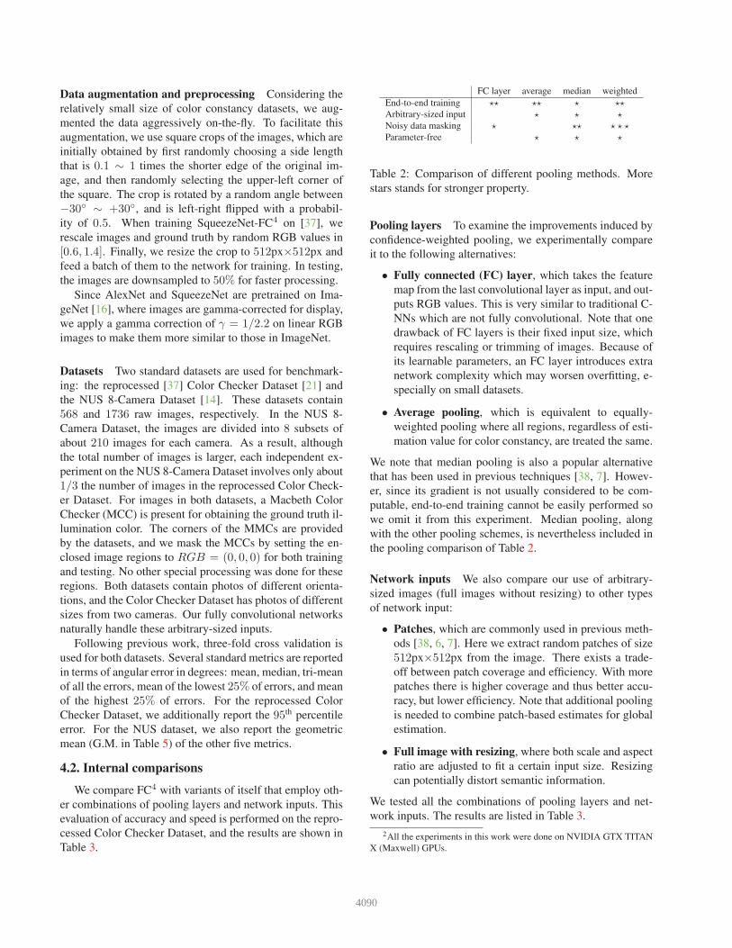
input image confidence map estimation map weighted estimation image × confidence estimation (left half) andground truth (right half)

Figure 3: Examples of outputs by our network. Note that noisy estimates in regions of little semantic value are masked by the

confidence map, resulting in more robust estimation. The angular errors are 0.54, 4.63, 1.78 and 4.76 degrees, respectively.

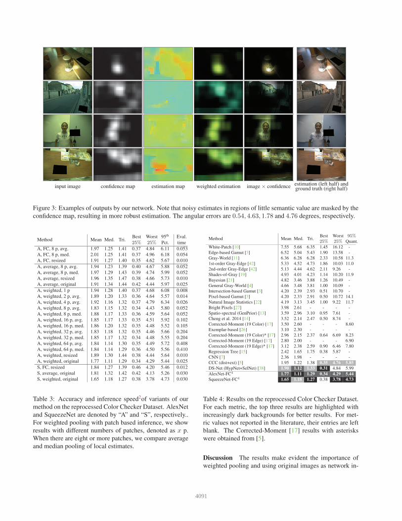
Method Mean Med. Tri.Best

25%Worst

25%95th

Pct.

Eval.

time

A, FC, 8 p, avg. 1.97 1.25 1.41 0.37 4.84 6.11 0.053

A, FC, 8 p, med. 2.01 1.25 1.41 0.37 4.96 6.18 0.054

A, FC, resized 1.91 1.27 1.40 0.35 4.62 5.67 0.010

A, average, 8 p, avg. 1.94 1.23 1.39 0.40 4.67 5.88 0.052

A, average, 8 p, med. 1.97 1.29 1.43 0.39 4.74 5.99 0.052

A, average, resized 1.96 1.35 1.47 0.38 4.66 5.73 0.010

A, average, original 1.91 1.34 1.44 0.42 4.44 5.97 0.025

A, weighted, 1 p 1.94 1.28 1.40 0.37 4.68 6.08 0.008

A, weighted, 2 p, avg. 1.89 1.20 1.33 0.36 4.64 5.57 0.014

A, weighted, 4 p, avg. 1.92 1.16 1.32 0.37 4.79 6.34 0.026

A, weighted, 8 p, avg. 1.83 1.15 1.32 0.34 4.43 5.80 0.052

A, weighted, 8 p, med. 1.88 1.17 1.33 0.36 4.59 5.64 0.052

A, weighted, 16 p, avg. 1.85 1.17 1.33 0.35 4.51 5.92 0.102

A, weighted, 16 p, med. 1.86 1.20 1.32 0.35 4.48 5.52 0.105

A, weighted, 32 p, avg. 1.83 1.18 1.32 0.35 4.46 5.66 0.204

A, weighted, 32 p, med. 1.85 1.17 1.32 0.34 4.48 5.55 0.204

A, weighted, 64 p, avg. 1.84 1.14 1.30 0.35 4.49 5.72 0.408

A, weighted, 64 p, med. 1.84 1.14 1.29 0.36 4.50 5.56 0.410

A, weighted, resized 1.89 1.30 1.44 0.38 4.44 5.64 0.010

A, weighted, original 1.77 1.11 1.29 0.34 4.29 5.44 0.025

S, FC, resized 1.84 1.27 1.39 0.46 4.20 5.46 0.012

S, average, original 1.81 1.32 1.42 0.42 4.13 5.26 0.030

S, weighted, original 1.65 1.18 1.27 0.38 3.78 4.73 0.030

Table 3: Accuracy and inference speed2of variants of our

method on the reprocessed Color Checker Dataset. AlexNet

and SqueezeNet are denoted by “A” and “S”, respectively..

For weighted pooling with patch based inference, we show

results with different numbers of patches, denoted as x p.

When there are eight or more patches, we compare average

and median pooling of local estimates.

Method Mean Med. Tri.Best

25%Worst

25%95%

Quant.

White-Patch [10] 7.55 5.68 6.35 1.45 16.12 -

Edge-based Gamut [3] 6.52 5.04 5.43 1.90 13.58 -

Gray-World [11] 6.36 6.28 6.28 2.33 10.58 11.3

1st-order Gray-Edge [42] 5.33 4.52 4.73 1.86 10.03 11.0

2nd-order Gray-Edge [42] 5.13 4.44 4.62 2.11 9.26 -

Shades-of-Gray [19] 4.93 4.01 4.23 1.14 10.20 11.9

Bayesian [21] 4.82 3.46 3.88 1.26 10.49 -

General Gray-World [4] 4.66 3.48 3.81 1.00 10.09 -

Intersection-based Gamut [3] 4.20 2.39 2.93 0.51 10.70 -

Pixel-based Gamut [3] 4.20 2.33 2.91 0.50 10.72 14.1

Natural Image Statistics [22] 4.19 3.13 3.45 1.00 9.22 11.7

Bright Pixels [27] 3.98 2.61 - - - -

Spatio-spectral (GenPrior) [13] 3.59 2.96 3.10 0.95 7.61 -

Cheng et al. 2014 [14] 3.52 2.14 2.47 0.50 8.74 -

Corrected-Moment (19 Color) [17] 3.50 2.60 - - - 8.60

Exemplar-based [26] 3.10 2.30 - - - -

Corrected-Moment (19 Color)* [17] 2.96 2.15 2.37 0.64 6.69 8.23

Corrected-Moment (19 Edge) [17] 2.80 2.00 - - - 6.90

Corrected-Moment (19 Edge)* [17] 3.12 2.38 2.59 0.90 6.46 7.80

Regression Tree [15] 2.42 1.65 1.75 0.38 5.87 -

CNN [7] 2.36 1.98 - - - -

CCC (dist+ext) [5] 1.95 1.22 1.38 0.35 4.76 5.85

DS-Net (HypNet+SelNet) [38] 1.90 1.12 1.33 0.31 4.84 5.99

AlexNet-FC4 1.77 1.11 1.29 0.34 4.29 5.44

SqueezeNet-FC4 1.65 1.18 1.27 0.38 3.78 4.73

Table 4: Results on the reprocessed Color Checker Dataset.

For each metric, the top three results are highlighted with

increasingly dark backgrounds for better results. For met-

ric values not reported in the literature, their entries are left

blank. The Corrected-Moment [17] results with asterisks

were obtained from [5].

Discussion The results make evident the importance of

weighted pooling and using original images as network in-

4091

Method Mean Med. Tri.Best

25%Worst

25%G.M.

White-Patch [10] 10.62 10.58 10.49 1.86 19.45 8.43

Edge-based Gamut [3] 8.43 7.05 7.37 2.41 16.08 7.01

Pixel-based Gamut [3] 7.70 6.71 6.90 2.51 14.05 6.60

Intersection-based Gamut [3] 7.20 5.96 6.28 2.20 13.61 6.05

Gray-World [11] 4.14 3.20 3.39 0.90 9.00 3.25

Bayesian [21] 3.67 2.73 2.91 0.82 8.21 2.88

Natural Image Statistics [22] 3.71 2.60 2.84 0.79 8.47 2.83

Shades-of-Gray [19] 3.40 2.57 2.73 0.77 7.41 2.67

Spatio-spectral (ML) [13] 3.11 2.49 2.60 0.82 6.59 2.55

General Gray-World [4] 3.21 2.38 2.53 0.71 7.10 2.49

2nd-order Gray-Edge [42] 3.20 2.26 2.44 0.75 7.27 2.49

Bright Pixels [27] 3.17 2.41 2.55 0.69 7.02 2.48

1st-order Gray-Edge [42] 3.20 2.22 2.43 0.72 7.36 2.46

Spatio-spectral (GenPrior) [13] 2.96 2.33 2.47 0.80 6.18 2.43

Corrected-Moment* (19 Edge) [17] 3.03 2.11 2.25 0.68 7.08 2.34

Corrected-Moment* (19 Color) [17] 3.05 1.90 2.13 0.65 7.41 2.26

Cheng et al. [14] 2.92 2.04 2.24 0.62 6.61 2.23

CCC (dist+ext) [5] 2.38 1.48 1.69 0.45 5.85 1.74

Regression Tree [15] 2.36 1.59 1.74 0.49 5.54 1.78

DS-Net (HypNet+SelNet) [38] 2.24 1.46 1.68 0.48 6.08 1.74

AlexNet-FC4 2.12 1.53 1.67 0.48 4.78 1.66

SqueezeNet-FC4 2.23 1.57 1.72 0.47 5.15 1.71

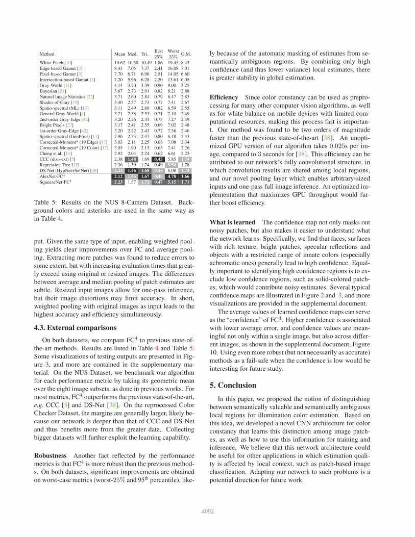
Table 5: Results on the NUS 8-Camera Dataset. Back-

ground colors and asterisks are used in the same way as

in Table 4.

put. Given the same type of input, enabling weighted pool-

ing yields clear improvements over FC and average pool-

ing. Extracting more patches was found to reduce errors to

some extent, but with increasing evaluation times that great-

ly exceed using original or resized images. The differences

between average and median pooling of patch estimates are

subtle. Resized input images allow for one-pass inference,

but their image distortions may limit accuracy. In short,

weighted pooling with original images as input leads to the

highest accuracy and efficiency simultaneously.

4.3. External comparisons

On both datasets, we compare FC4 to previous state-of-

the-art methods. Results are listed in Table 4 and Table 5.

Some visualizations of testing outputs are presented in Fig-

ure 3, and more are contained in the supplementary ma-

terial. On the NUS Dataset, we benchmark our algorithm

for each performance metric by taking its geometric mean

over the eight image subsets, as done in previous works. For

most metrics, FC4 outperforms the previous state-of-the-art,

e.g. CCC [5] and DS-Net [38]. On the reprocessed Color

Checker Dataset, the margins are generally larger, likely be-

cause our network is deeper than that of CCC and DS-Net

and thus benefits more from the greater data. Collecting

bigger datasets will further exploit the learning capability.

Robustness Another fact reflected by the performance

metrics is that FC4 is more robust than the previous method-

s. On both datasets, significant improvements are obtained

on worst-case metrics (worst-25% and 95th percentile), like-

ly because of the automatic masking of estimates from se-

mantically ambiguous regions. By combining only high

confidence (and thus lower variance) local estimates, there

is greater stability in global estimation.

Efficiency Since color constancy can be used as prepro-

cessing for many other computer vision algorithms, as well

as for white balance on mobile devices with limited com-

putational resources, making this process fast is importan-

t. Our method was found to be two orders of magnitude

faster than the previous state-of-the-art [38]. An unopti-

mized GPU version of our algorithm takes 0.025s per im-

age, compared to 3 seconds for [38]. This efficiency can be

attributed to our network’s fully convolutional structure, in

which convolution results are shared among local regions,

and our novel pooling layer which enables arbitrary-sized

inputs and one-pass full image inference. An optimized im-

plementation that maximizes GPU throughput would fur-

ther boost efficiency.

What is learned The confidence map not only masks out

noisy patches, but also makes it easier to understand what

the network learns. Specifically, we find that faces, surfaces

with rich texture, bright patches, specular reflections and

objects with a restricted range of innate colors (especially

achromatic ones) generally lead to high confidence. Equal-

ly important to identifying high confidence regions is to ex-

clude low confidence regions, such as solid-colored patch-

es, which would contribute noisy estimates. Several typical

confidence maps are illustrated in Figure 2 and 3, and more

visualizations are provided in the supplemental document.

The average values of learned confidence maps can serve

as the “confidence” of FC4. Higher confidence is associated

with lower average error, and confidence values are mean-

ingful not only within a single image, but also across differ-

ent images, as shown in the supplemental document, Figure

10. Using even more robust (but not necessarily as accurate)

methods as a fail-safe when the confidence is low would be

interesting for future study.

5. Conclusion

In this paper, we proposed the notion of distinguishing

between semantically valuable and semantically ambiguous

local regions for illumination color estimation. Based on

this idea, we developed a novel CNN architecture for color

constancy that learns this distinction among image patch-

es, as well as how to use this information for training and

inference. We believe that this network architecture could

be useful for other applications in which estimation quali-

ty is affected by local context, such as patch-based image

classification. Adapting our network to such problems is a

potential direction for future work.

4092

References

[1] M. Abadi, A. Agarwal, P. Barham, E. Brevdo, Z. Chen, C. C-

itro, G. S. Corrado, A. Davis, J. Dean, M. Devin, S. Ghe-

mawat, I. Goodfellow, A. Harp, G. Irving, M. Isard, Y. Jia,

R. Jozefowicz, L. Kaiser, M. Kudlur, J. Levenberg, D. Mane,

R. Monga, S. Moore, D. Murray, C. Olah, M. Schuster,

J. Shlens, B. Steiner, I. Sutskever, K. Talwar, P. Tucker,

V. Vanhoucke, V. Vasudevan, F. Viegas, O. Vinyals, P. War-

den, M. Wattenberg, M. Wicke, Y. Yu, and X. Zheng. Tensor-

Flow: Large-scale machine learning on heterogeneous sys-

tems, 2015. Software available from tensorflow.org. 5

[2] A. Alemi. Improving inception and image classification in

tensorflow. https://research.googleblog.com/

2016/08/improving-inception-and-image.

html. 4

[3] K. Barnard. Improvements to gamut mapping colour con-

stancy algorithms. In European Conference on Computer

Vision, pages 390–403. Springer, 2000. 7, 8

[4] K. Barnard, L. Martin, A. Coath, and B. Funt. A comparison

of computational color constancy algorithms. ii. experiments

with image data. IEEE Transactions on Image Processing,

11(9):985–996, 2002. 7, 8

[5] J. T. Barron. Convolutional color constancy. In International

Conference on Computer Vision, pages 379–387, 2015. 1, 2,

3, 7, 8

[6] S. Bianco, C. Cusano, and R. Schettini. Color constancy us-

ing cnns. In Computer Vision and Pattern Recognition Work-

shops, pages 81–89, 2015. 1, 2, 3, 6

[7] S. Bianco, C. Cusano, and R. Schettini. Single and multiple

illuminant estimation using convolutional neural networks.

ArXiv e-prints, 1508.00998, 2015. 1, 2, 3, 4, 6, 7

[8] S. Bianco and R. Schettini. Color constancy using faces.

In Computer Vision and Pattern Recognition, pages 65–72.

IEEE, 2012. 2

[9] S. Bianco and R. Schettini. Adaptive color constancy using

faces. IEEE Transactions on Pattern Analysis and Machine

Intelligence, 36(8):1505–1518, 2014. 2

[10] D. H. Brainard and B. A. Wandell. Analysis of the retinex

theory of color vision. JOSA A, 3(10):1651–1661, 1986. 7,

8

[11] G. Buchsbaum. A spatial processor model for object colour

perception. Journal of the Franklin Institute, 310(1):1–26,

1980. 2, 7, 8

[12] V. C. Cardei, B. Funt, and K. Barnard. Estimating the scene

illumination chromaticity by using a neural network. JOSA

A, 19(12):2374–2386, 2002. 2

[13] A. Chakrabarti, K. Hirakawa, and T. Zickler. Color constan-

cy with spatio-spectral statistics. IEEE Transactions on Pat-

tern Analysis and Machine Intelligence, 34(8):1509–1519,

2012. 7, 8

[14] D. Cheng, D. K. Prasad, and M. S. Brown. Illuminant estima-

tion for color constancy: why spatial-domain methods work

and the role of the color distribution. JOSA A, 31(5):1049–

1058, 2014. 6, 7, 8

[15] D. Cheng, B. Price, S. Cohen, and M. S. Brown. Effective

learning-based illuminant estimation using simple features.

In Computer Vision and Pattern Recognition, pages 1000–

1008, 2015. 2, 7, 8

[16] J. Deng, W. Dong, R. Socher, L.-J. Li, K. Li, and L. Fei-

Fei. Imagenet: A large-scale hierarchical image database. In

Computer Vision and Pattern Recognition, pages 248–255.

IEEE, 2009. 4, 6

[17] G. D. Finlayson. Corrected-moment illuminant estima-

tion. In International Conference on Computer Vision, pages

1904–1911, 2013. 7, 8

[18] G. D. Finlayson, S. D. Hordley, and P. M. Hubel. Color

by correlation: A simple, unifying framework for color con-

stancy. IEEE Transactions on Pattern Analysis and Machine

Intelligence, 23(11):1209–1221, 2001. 2

[19] G. D. Finlayson and E. Trezzi. Shades of gray and colour

constancy. In Color and Imaging Conference, volume 2004,

pages 37–41. Society for Imaging Science and Technology,

2004. 7, 8

[20] B. Funt and W. Xiong. Estimating illumination chromaticity

via support vector regression. In Color and Imaging Confer-

ence, volume 2004, pages 47–52. Society for Imaging Sci-

ence and Technology, 2004. 2

[21] P. V. Gehler, C. Rother, A. Blake, T. Minka, and T. Sharp.

Bayesian color constancy revisited. In Computer Vision and

Pattern Recognition, pages 1–8. IEEE, 2008. 1, 6, 7, 8

[22] A. Gijsenij and T. Gevers. Color constancy using natural

image statistics and scene semantics. IEEE Transactions on

Pattern Analysis and Machine Intelligence, 33(4):687–698,

2011. 7, 8

[23] A. Gijsenij, T. Gevers, and J. Van De Weijer. Computational

color constancy: Survey and experiments. IEEE Transac-

tions on Image Processing, 20(9):2475–2489, 2011. 2

[24] S. D. Hordley. Scene illuminant estimation: past, present,

and future. Color Research & Applications, 31(4):303–314,

2006. 2

[25] F. N. Iandola, S. Han, M. W. Moskewicz, K. Ashraf, W. J.

Dally, and K. Keutzer. Squeezenet: Alexnet-level accuracy

with 50x fewer parameters and < 0.5 mb model size. ArXiv

e-prints, 1602.07360, 2016. 5

[26] H. R. V. Joze and M. S. Drew. Exemplar-based color constan-

cy and multiple illumination. IEEE Transactions on Pattern

Analysis and Machine Intelligence, 36(5):860–873, 2014. 7

[27] H. R. V. Joze, M. S. Drew, G. D. Finlayson, and P. A. T.

Rey. The role of bright pixels in illumination estimation. In

Color and Imaging Conference, volume 2012, pages 41–46.

Society for Imaging Science and Technology, 2012. 7, 8

[28] D. Kingma and J. Ba. Adam: A method for stochastic op-

timization. In International Conference on Learning Repre-

sentations, 2015. 5

[29] A. Krizhevsky, I. Sutskever, and G. E. Hinton. Imagenet

classification with deep convolutional neural networks. In

Advances in Neural Information Processing Systems, pages

1097–1105, 2012. 4

[30] J. Long, E. Shelhamer, and T. Darrell. Fully convolution-

al networks for semantic segmentation. In Computer Vision

and Pattern Recognition, pages 3431–3440, 2015. 3

[31] Z. Lou, T. Gevers, N. Hu, and M. P. Lucassen. Color constan-

cy by deep learning. In British Machine Vision Conference,

2015. 1, 2, 3, 4

4093

[32] D. Pathak, P. Krahenbuhl, and T. Darrell. Constrained con-

volutional neural networks for weakly supervised segmenta-

tion. In International Conference on Computer Vision, 2015.

3

[33] D. Pathak, E. Shelhamer, J. Long, and T. Darrell. Fully con-

volutional multi-class multiple instance learning. In Interna-

tional Conference on Learning Representations, 2015. 3

[34] S. E. Reed, H. Lee, D. Anguelov, C. Szegedy, D. Erhan,

and A. Rabinovich. Training deep neural networks on noisy

labels with bootstrapping. In International Conference on

Learning Representations, 2015. 2, 3

[35] C. Rosenberg, M. Hebert, and S. Thrun. Color constancy us-

ing kl-divergence. In International Conference on Computer

Vision, volume 1, pages 239–246. IEEE, 2001. 2

[36] E. Shelhamer, J. Long, and T. Darrell. Fully convolutional

networks for semantic segmentation. IEEE Transactions on

Pattern Analysis and Machine Intelligence, 39(4):640–651,

2017. 3

[37] L. Shi and B. Funt. Re-processed version of the gehler color

constancy dataset of 568 images. http://www.cs.sfu.

ca/˜colour/data/. 6

[38] W. Shi, C. C. Loy, and X. Tang. Deep specialized network for

illuminant estimation. In European Conference on Computer

Vision, pages 371–387. Springer, 2016. 1, 2, 3, 4, 5, 6, 7, 8

[39] K. Simonyan and A. Zisserman. Very deep convolutional

networks for large-scale image recognition. In International

Conference on Learning Representations, 2015. 4

[40] N. Srivastava, G. E. Hinton, A. Krizhevsky, I. Sutskever, and

R. Salakhutdinov. Dropout: a simple way to prevent neu-

ral networks from overfitting. Journal of Machine Learning

Research, 15(1):1929–1958, 2014. 5

[41] S. Sukhbaatar, J. Bruna, M. Paluri, L. Bourdev, and R. Fer-

gus. Training convolutional networks with noisy labels.

In International Conference on Learning Representations,

2015. 2, 3

[42] J. Van De Weijer, T. Gevers, and A. Gijsenij. Edge-based

color constancy. IEEE Transactions on Image Processing,

16(9):2207–2214, 2007. 2, 7, 8

[43] T. Xiao, T. Xia, Y. Yang, C. Huang, and X. Wang. Learning

from massive noisy labeled data for image classification. In

Computer Vision and Pattern Recognition, 2015. 2, 3

4094