Fault-tolerant meshes and hypercubes with minimal numbers ...

IEEE TRANSACTIONS ON COMPUTERS, VOL. 42, NO. 9. SEPTEMBEK lYY3 10x9

Fault-Tolerant Meshes and Hypercubes with Minimal Numbers of Spares

Jehoshua Bruck, Robert Cypher, and Ching-Tien Ho, Member, IEEE

Abstract-Many parallel computers consist of processors connected in the form of a d-dimensional mesh or hypercube. Two- and three-dimensional meshes have been shown to be efficient in manipulating images and dense matrices, whereas hypercubes have been shown to be well suited to divide-and- conquer algorithms requiring global communication. However, even a single faulty processor or communication link can seriously affect the performance of these machines.

This paper presents several techniques for tolerating faults in tl-dimensional mesh and hypercube architectures. Our approach consists of adding spare processors and communication links so that the resulting architecture will contain a fault-free mesh or hypercube in the presence of faults. We optimize the cost of the fault-tolerant architecture by adding exactly k spare processors (while tolerating up to k processor and/or link faults) and minimizing the maximum number of links per processor. For example, when the desired architecture is a d-dimensional mesh and !i = 1, we present a fault-tolerant architecture that has the same maximum degree as the desired architecture (namely, 2tl) and has only one spare processor. We also present efficient layouts for fault-tolerant two- and three-dimensional meshes, and show how multiplexers and buses can be used to reduce the degree of fault-tolerant architectures. Finally, we give constructions for fault-tolerant tori, eight-connected meshes, and hexagonal meshes.

I. INTRODUCTION

ANY existing parallel machines have a mesh or hy- M percube topology. Examples of hypercube computers include the Cosmic Cube (from Caltech), the iPSC/860 (from Intel), the NCUBE (from NCUBE Inc.), and the CM-2 (from Thinking Machines). Examples of two-dimensional mesh computers include the MPP (from Goodyear Aerospace) [3], the MP-1 (from MASPAR), VICTOR (from IBM), and DELTA (from Intel and Caltech). The J-Machine, which is under development at MIT, and the GC series from Parsytec [20] are three-dimensional meshes. In addition, memory chips are also organized in the form of a two-dimensional mesh [16],

As improvements in technology lead to the creation of larger parallel computers, it becomes essential to consider the issue of computing in the presence of faults. In particular, the ability to

1271.

Manuscript received July 2, 1991; revised November 12, 1991, and August 28, 1992. This work is based on “Fault-Tolerant Meshes with Minimal Numbers of Spares,’’ by J. Bruck, R. Cypher, and C. T. Ho, which appeared in the Proceedings of the 3rd IEEE Symposium on Parallel und Distributed Processing, Dallas, TX, Dec. 2-5, 1991, pp. 288-295, and “Efficient Fault-Tolerant Mesh and Hypercube Architectures,” which appeared in the Proceedings of the 22nd Annual International Symposium on Fault-Tolerunt Computing, Boston, MA, July 8-10, 1992, pp. 162-169. 01991, 1992 IEEE.

The authors are with IBM, Almaden Research Center, San Jose. CA 95120. IEEE Log Number 9208568.

tolerate even a small number of faults could allow the machine to be used between the time a failure is first detected and the time the machine is repaired. As a result, several existing parallel machines contain spare processors and are designed to tolerate a limited number of faults [3], [20].

A large amount of research has been devoted to creating fault-tolerant parallel architectures. The techniques used in this research can be divided into two main classes. The first class consists of techniques that do not add redundancy to the desired architecture. Instead, these techniques attempt to mask the effects of faults by using the healthy part of the architecture to simulate the entire machine [l], [6], [12], [14]. The hope with this approach is to obtain the same functionality with a reasonable slowdown factor. Although this approach yields interesting theoretical results, even a constant factor slowdown in performance can be very significant in practice. Furthermore, this approach requires that some healthy processors simulate several processors. As a result, each simulated processor can have only a fraction of the memory present in a healthy processor.

The second class consists of techniques that do add redundancy to the desired architecture. These techniques attempt to isolate the faults, usually by disabling certain links or disallowing certain switch settings, while maintaining the complete desired architecture [2], [3], [SI, [8]-[ lo], [13], [ 1S]-[17], [ 191, [21]-[24], [26], [28]. Many of these techniques require either a nonminimal number of spare processors [2], [3], [SI, [lS], [16], [24], [26] or a switching mechanism assumed to be immune to faults [3], [lS], [16], [21], [22], [24], [26]. In contrast, the results presented herein use only the minimal number of spare processors and can tolerate faults in any of the components. Finally, we assume a worst case distribution of faults, whereas many of the preceding approaches do not work in a worst case scenario.

Our approach is based on a graph model. In this model a distributed memory parallel computer is viewed as being a graph in which the nodes represent the processors and the edges represent the communication links. A target graph with 71 nodes is selected first. Then a fault-tolerant graph with 72 + k: nodes is defined with the property that, given any set of A. or fewer faulty nodes, the remaining graph is guaranteed to contain the target graph as a subgraph. This approach guarantees that any algorithm designed for the target graph will run with no slowdown in the presence of k . or fewer node faults, regardless of their distribution. Note that in our approach the spare nodes are fully utilized. Hence, minimizing the cost in this model amounts to constructing a fault-tolerant graph with

0018-93-10/93$03.00 0 1903 IEEE

I 1 90 IEEE TRANSACTIONS ON COMPUTERS, VOL. 42, NO. 9, SEPTEMBER 1933

a small maximum degree. Although our results are stated for n>de faults, it should be noted that they can also be used t o tolerate edge faults by viewing a node incident with each I iulty edge as being faulty.

This graph model of fault tolerance has been used by several I ther researchers. Hayes [13] has used this model with target p raphs of cycles, linear arrays, and trees. Rosenberg examined 1 iult-tolerant graphs for linear arrays [ 2 3 ] . The work by Wong ‘1 nd Wong [28] and Paoli et al. [ 191 relates to cycles. The more r:cent work by Dutt and Hayes uses trees [8], hypercubes [9], I. irculant and nearly circulant graphs [9], and arbitrary graphs

The main contribution of this paper is the creation of effi- 1. ient fault-tolerant graphs for several important target graphs.

pecifically, we give four different constructions for creating I iult-tolerant two-dimensional meshes, as well as constructions I 3r creating fault-tolerant d -dimensional meshes, hypercubes, t x i , eight-connected meshes, and hexagonal meshes. In all <ases. our fault-tolerant graphs have a smaller degree than I ny previously known graphs with the same properties. In I articular, we present a construction for fault-tolerant d- imensional meshes that can tolerate k faults and has degree

i k + 1)d when k is odd and ( k + 2)d when k is even. ‘hus when k = 1 this construction has degree 2d, which

I S no larger than the degree of the target graph. Our fault- t alerant graph for the d-dimensional hypercube has degree ik + 2)d - ( k + 2)log k + 2k - 3 when k is a power of

1. This is approximately a factor of 2 improvement over the result obtained by Dutt and Hayes, which has degree ! ( ( k + 1)d- ( k + 1) log k - 3 ) when k is a power of 2 [9]. We llso show how multiplexers and buses can be used to reduce he degree of the fault-tolerant architectures.

The rest of this paper is organized as follows. Defini- ions that will be used throughout the paper are given in iection 11. In Section 111, we present several fault-tolerant wo-dimensional meshes, all of which are based on a family If graphs known as “circulant graphs.” In Section IV, we ntroduce another family of graphs, called “diagonal graphs,” ind show how they can be used to create fault-tolerant d- limensional meshes and hypercubes. We also present efficient mplementations for many of these fault-tolerant architectures. Section V shows how the same techniques can be used to sreate fault-tolerant graphs for target graphs that are related to he mesh. Conclusions are presented in Section VI.

IO] as target graphs.

11. DEFINITIONS

The following definitions will be used throughout this paper. Definition: Let IC be a nonnegative integer and let G =

(V,E) be a graph. We say that the graph G’ = (V’,E’) is (k,G)-tolerant if the subgraph of G’ induced by any set of IV’I - k nodes contains G as a subgraph. We note here that throughout this paper the number of spare nodes is minimal,

Definition: Given two graphs G1 and G2: a function of 4 that maps the vertices of G1 to the vertices of G2 is called an embedding of GI into G2 if for any pair of distinct

so JV’J = J V J + I C .

0

12 4

8

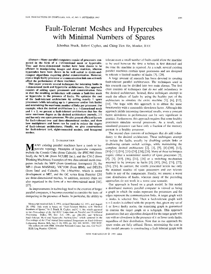
Fig. 1. Circulant graph with 16 nodes and offsets 1 and 4.

nodes i and j in G I , qb(1:) # qb(j), and for any edge ( i , j ) in G l , ( d ( i ) , b ( j ) ) is an edge in Gz.

Definition: For any positive integer n, the set { O , 1 , . . . , n - 1) will be denoted [n].

Definition: Let nn,ni,”.,nd-l be integers all of which are greater than or equal to 2. The no x ‘11 x . . . n d - 1 d- dimensional mesh M consists of IIfzt n,; nodes. Each node in M has a unique label of the form (an, (11, . . , ad-1) whcre for all 1: E [ d ,a i E [nil. Each node ( a o , a l ; . . . > a d - l ) is connected to the 2d other nodes of the form (an, . . . , ai- 1, n f 1, ai+l,. . . , a d - 1 ) provided they exist.

Definition: The d-dimensional hypercube, denoted Qd, i; a 2 x 2 x . . . x 2 d-dimensional mesh with n = 2d nodes. Note that hypercubes are simply special types of d-dimensional mesh-s, so that results presented for d-dimensional meshes will apply to d-dimensional hypercubes as well.

111. CIRCULANT GRAPHS

This section discusses a class of graphs known as “circul int graphs” [ll] and shows how they can be used to create fault-tolerant two-dimensional meshes. We begin by defin ng circulant graphs and reviewing some of their known properties.

Definition: Let p be a positive integer and let S be a set of integers in the range 1 through p - 1. The p -node c i rcuht graph with connection set S , denoted C,,S, consists of p nodes. Each node in C,,S has a unique label in the range 0 throi.gh p - 1. Each node 1: is connected to all nodes of the form ( z 4: s) mod p where s E S. The values in the connection set S will be referred to as ‘‘jumps’’ or “offsets.” A simple example c f a circulant graph is a cycle, where there is only one offset and the value of that offset is 1. Fig. 1 shows an example cf a circulant graph.

Definition: Let p be a positive integer and let S be a se of integers in the range 1 through p - 1. The closure of S b)! p , denoted close( S , p ) , is the set

T = {t( t E S or ( p - t ) 5)

Note that the degree of C,,S is ( c l o s e ( S . p ~ ( . In addition, note that IS1 5 Iclose(S,p)l 5 2(SI.

Definition: Let S be a set of integers and let k be a nonceg- ative integer. The expansion of S by I C , denoted expand(S. k),

BRUCK et al.: FAULT-TOLERANT MESHES AND HYPERCUBES 1091

is the set T , where

Note that lezpand(S,k)( 5 ( k + 1)lSl. The following theorem is an immediate consequence of a

result proven by Dutt and Hayes [9]. Theorem 3.1 [9]: Let n be a positive integer, let S be a

set of integers in the range 1 through n - 1, let k be a nonnegative integer, and let T = ezpand(S, k ) . The circulant graph Cn+k,T is ( k , C,,s)-tolerant.

The idea behind Theorem 3.1 is that given any set of k faulty nodes in Cn+k ,T , we can embed the target graph cn,s into the healthy nodes of the fault-tolerant graph Cn+k,T by mapping each node i in the target graph to the ith healthy node in the fault-tolerant graph. It is clear that any pair of nodes that are z apart in the target graph are mapped to nodes in the fault-tolerant graph that are at least z apart and at most z + k apart (because there are between 0 and k faulty nodes between them). Consider any edge that connects nodes that are z apart in the target graph, where z E S. This edge will be mapped to nodes that are z’ apart in the fault-tolerant graph, where z’ E T , so it will be mapped to an edge in the fault-tolerant graph.

Theorem 3.1 gives a general technique for creating a fault- tolerant graph when the target graph is circulant. We will use Theorem 3.1 to obtain four different constructions for fault-tolerant two-dimensional meshes. Each construction first defines a circulant graph, which is a supergraph of the desired two-dimensional mesh. Then Theorem 3.1 is used to add fault tolerance to the supergraph. It is interesting to note that circulant graphs that contain two-dimensional meshes as subgraphs have been studied in a context unrelated to fault tolerance [4].

Throughout the remainder of this section, let T and c be integers greater than or equal to 2, and let k be a nonnegative integer. Additional constraints on these parameters will be added as needed. In addition, let Mr,c denote the two-dimensional mesh with T rows and c columns. The four different constructions and their degrees are given in Theorems 3.3, 3.5, 3.7, and 3.14. Another construction for fault-tolerant two-dimensional meshes is given in Corollary 4.7 in Section IV. This final construction has the smallest degree when the number of faults that must be tolerated is small.

A. Mesh Construction 1

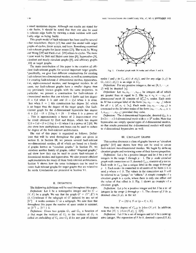
The first fault-tolerant mesh construction is based on the fact that, when the nodes in Mr,c are labeled in row-major order, the labels of adjacent nodes differ by either 1 or c [see Fig. 2(a)].

Lemma 3.2: Let S = { 1, c}. The mesh Mr,c is a subgraph of the circulant graph CrC,s.

Proof: Let q5(i,j) = i c + j . It is straightforward to verify 0

Theorem 3.3: Let S = { 1, c} and let T = expand( S , k ) . The circulant graph Crc+k,T is ( k , M,,,)-tolerant and has degree at most 4k + 4.

that q5 defines an embedding of Mr,c into CrC,s.

l ! ! ! ! ! ! ! l

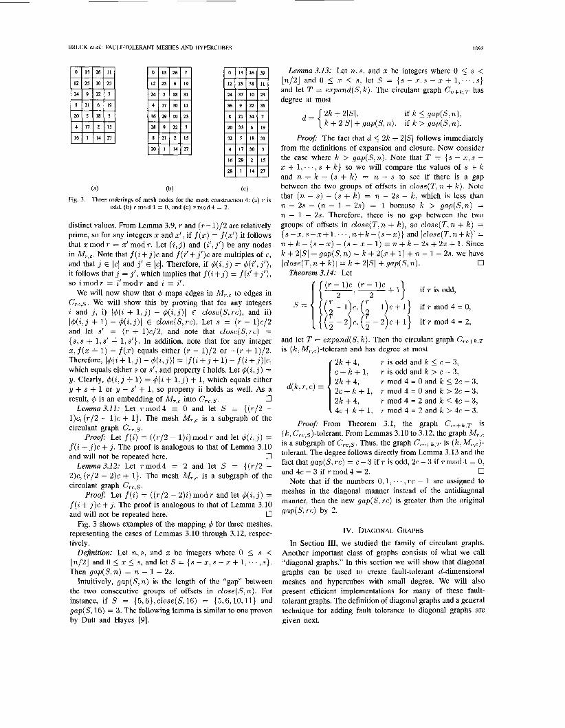
@2l@l8@22@l7@Z2@17@U@ M 19 21 I8 21 18 21 18 @18@U@17@22@17@22@17@ 19 21 18 21 18 21 18 21 aUm17.U.17 .Pm17mU. 21 18 21 18 21 18 21 19 @17@22@17@U@17@U@18@ 18 21 18 21 18 21 19 M @a@ l7@22@ 17@U@ 18@2l

(c) ( 4

Fig. 2. Three orderings of mesh nodes

Proof: From Theorem 3.1, the graph Crc+k,T is (k,C,,,s)-tolerant. From Lemma 3.2, the graph Mr,c is a subgraph of cTc,s. As a result, the graph Crc+k,T is ( k , M r , c ) -

tolerant. Because IS1 5 2 and T = ezpand(S, k ) , (TI 5 2 k f 2 0 and the degree of Crc+k,T is at most 4k + 4.

B. Mesh Construction 2 Whereas Construction 1 is a very natural application of

Theorem 3.1, Theorem 3.1 can also be used to obtain more efficient constructions. We will now give a construction for obtaining a graph that tolerates k faults and has degree only 2k + 4. This construction is based on an ordering of the nodes in the mesh that we call the antidiagonal-major order [see Fig. 2(b)]. The advantage of antidiagonal-major order is that it leads to a circulant graph that has a connection set consisting of two consecutive integers. As a result, fault tolerance can be added to the circulant graph in an efficient manner.

Lemma 3.4: Let S = {c, c + 1). The mesh Mr,c is a subgraph of the circulant graph Crc,s.

Proof: Let I$ ( i , j ) = ( ( i + j) mod T ) C + j. It is straightforward to verify that I$ defines an embedding of MT,c into

Theorem 3.5: Let S = {c, c+l} and let T = ezpand(S, k ) . The circulant graph Crc+k,T is ( k , M,,,)-tolerant and has degree at most 2k + 4.

Proof: From Theorem 3.1, the graph Crc+k,T is (k,C,,,s)-tolerant. From Lemma 3.4, the graph Mr,c is a subgraph of CTC,s. As a result, the graph Crc+k,T is (k, tolerant. BecauseT = { c , c + l , ~ ~ ~ , c + k + l } , ~ T ~ 5 k + 2

0

crc,s 0

and the degree of Crc+k,T is at most 2k + 4.

C. Mesh Construction 3 The fault-tolerant meshes produced by Construction 2 re-

quire two additional edges per node for each additional fault that is tolerated. We will now give a construction that requires only one additional edge per node for each additional fault that is tolerated. However, this reduced rate of growth in the degree requires a larger initial degree.

The construction is based on an ordering of the nodes in the mesh that we call the interleaved antidiagonal-major order [see Fig. 2(c)]. The interleaved antidiagonal-major order

1092 IEEE TRANSACTIONS ON COMPUTERS, VOL. 42, NO. 9, SEPTEMBER 993

issigns the numbers 0 through r c - 1 to the nodes in M,,c. Yode (0, 0) (the upper left corner) is assigned the value 0, and successive values are assigned to the nodes in every 3ther antidiagonal. Then node (1, 0) (the node immediately below the upper left comer) is assigned the value [rc/2], and successive values are assigned to the nodes in the remaining antidiagonals. The advantage of interleaved antidiagonal-major order is that it leads to a circulant graph with r c nodes that has a connection set clustered about the value rc/2.

Lemma 3.6: Let r and c be integers greater than 2, let a = [rc/21 - [r/2], let b = [rc/2] + Lr/2], and let S be the set of integers in the range a through b. The mesh M,,, is a subgraph of the circulant graph CTC,s.

Proof: Let d ( i , j ) be the value assigned to node ( i , j ) when M,,, is labeled in interleaved antidiagonal-major order. It will be shown that for any nodes ( i1 , j l ) and ( i 2 , j z ) that are adjacent in M,,,,a 5 I4(il , j l) - 4 ( 2 2 , j 2 ) 1 I 6 .

For all integers i and j where 0 5 i 5 r - 1 and 0 I j < c - 1, let hi,j = I4( i , j ) - 4( i , j + 1)l. For all integers i and j where 0 5 i < r - 1 and 0 5 j 5 c - 1, let ui,j = I4( i , j ) - d(Z + 1, j ) l . We will call the hi,j values horizontal differences and the ui, j values vertical differences [see Fig. 2(d)]. First, we will show that if there is a vertical difference that is not in the range a through b, then there is also a horizontal difference that is not in the range a through b. Let ui,j be any vertical difference. If j = 0 then either hi,j < ui, j < hi+l,j or hi+l,j < ui, j < hi>j. Conversely, if j > 0 then either hi,j-l < ui,j < hi+l,j-l or hi+l,j-l < ui,j < hi,j-l. Therefore, if the ui,j is not in the range a through b, there also exists an hij,jf that is not in the range a through b.

It is clear that for all i and j where 1 5 i 5 r - 1 and 0 5 j I c - 3, hi,j = hi-l,j+l, so horizontal differences that are in the same antidiagonal are equal. It will be helpful to divide the horizontal differences into two sets according to their parity. We will say that horizontal difference hi,j is even if i + j is even, and it is odd otherwise. It is straightforward to show that all even horizontal differences are greater than rc/2 and all odd horizontal differences are less than rc/2. Furthermore, it is straightforward to show that the largest horizontal difference is hr-2,0 if r is even and h,-l,o if r is odd, whereas the smallest horizontal difference is h,-l,o if r is even and hr-2,0 if r is odd. Therefore, it suffices to show that hr-2,0 and h,-l,o are in the range a through b. There are two cases:

Case 1) r is even: In this case, 4(r - 2,O) = r2/4 - r + I , $(r - 2, I ) = rc/2 + r2 /4 - r /2 + 1, $(r - 1,O) = rc /2 + r 2 / 4 - r /2 , and 4(r - 1, l ) = r2/4. Thus, hr-2,0 = rc/2 + r / 2 = b and h,-l,o = rc/2 - r / 2 = a.

Case 2) r is odd: In this case, 4(r - 2,O) - [rc/21 + Lr/2]’ - Lr/2],4(r - 2 , l ) = Lr/212 + 1 , 4 ( ~ - 1 , O ) = Lr/2J2,4(r-1,1) = [rc/21+Lr/2j2+Lr/2j. Thus, hr-2,0 = [rc/2] - [r/2] = a and h,-l,o = [rc/21 + [r/2J = b.

It has been shown that all horizontal and vertical differences are in the range a through b. Furthermore, 4 assigns a unique value in the range 0 through r c - 1 to each node in M,,,. As a result, it follows that 4 defines an embedding of M,,, into C,, s.

Theorem 3.7: Let r and c be integers greater than 2, let a = rrc/21 - rr/21, let b = [rc/21 + Lr/2], let S be the set of integers in the range a through b, and let T = erpand(S, IC) . The circulant graph C,.c+k,T is ( k , M,,,)-tolerant and las degree at most k + r + 1 when r is odd and c is even, and at most k + r otherwise.

Proof: From Theorem 3.1, the graph Crc+k,T is (k,C,,,s)-tolerant. From Lemma 3.6, the graph M,., is, a subgraph of CTc,s. As a result, the graph C r c + k , T is ( k , M, C ) -

tolerant. Note that T = { a , a + l , . . . , b + k } and that b-a = r. If r is odd and c is even, then close(T, rc + k) = { a , L + 1 , . . - , b+k+l} and the degree of C,c+k,T is at most k+r-- l . Otherwise, close(T, rc + k) = { a , a + 1 , . . . , b + I C } and the

Theorem 3.7 is based on Lemma 3.6, which showed that the mesh My,, is a subgraph of a circulant graph with r c nodes and a connection set that has values near rc/2. Specifically, when r is odd and c is even, all of the values in the connection set are within ( r+1) /2 of rc/2, and in all other cases all of the values in the connection set are within r /2 of rc/2. If Lemma 3.6 could be improved by finding a circulant graph wit’i a connection set that is more tightly clustered around rc/2, the degree of the construction in Theorem 3.7 could be reduced. However, as we will see in Theorem 3.8, no such improvement in Lemma 3.6 is possible. The proof of Theorem 3.8 is gkien in the Appendix.

Theorem 3.8: Let r and c be integers where 4 5 r 5 c md let CTC,s be a circulant graph that contains the mesh M,.,, ;is a subgraph. There exists an s E S such that 1s - (rc/2)1 2 ( r + 1)/2 if r is odd and c is even, and such that 1s - (rc/2)1 2 -/2 otherwise.

degree of CTc+k,T is at most k + r.

D. Mesh Construction 4

We will now present constructions of ( k , M,,,)-tolelant graphs that combine the advantages of Constructions 2 md 3. More precisely, the degree of the construction given l-ere increases at the rate of two per fault up to some number of faults, at which point it increases at the rate of one per fault. The cut-off point at which the rate of growth in the degree slows depends on a value called the gap, which will be defined later.

Lemma 3.9: The following properties hold. i) If r is 1)dd then r and ( r - l ) / 2 are relatively prime. ii) If T mod 4 = 0 then r and (r /2) - 1 are relatively prime. iii) If r m o d 4 = 2 then r and ( r /2) - 2 are relatively prime.

Proof: First, we prove i). Let r = 22 + 1 when: 5

is an integer. Thus gcd( r , ( r - 1)/2) = gcd(22 + 1 9 x ; = gcd( 1, 2 ) = 1, so r and ( r - 1)/2 are relatively prime. To prove ii), let r = 42 where 2 is an integer. Thus gcd(r, ( r /2) - 1) = gcd(4z,22 - 1) = gcd(2,2z - 1) = 1. To prove iii), let r = 42 + 2 where 2 is an integer. Thus, gcd(r , ( r /2) - 2) =

Lemma 3.10: Let r be odd and let S = { ( r - l)c/2, ( r - l )c /2 + l}. The mesh M,,, is a subgraph of the circulant

Proof: Let f ( i ) = ( i ( r - 1) /2 )modr and let $ ( i , j ) = f ( i + j ) c + j . First, we will show that 4 maps distinct nodes to

g c d ( 4 ~ + 2,22 - 1) = gcd(4,22 - 1) = 1.

graph CTr,s.

BRUCK et al.: FAULT-TOLERANT MESHES AND HYPERCUBES 1093

(a) (b) (c)

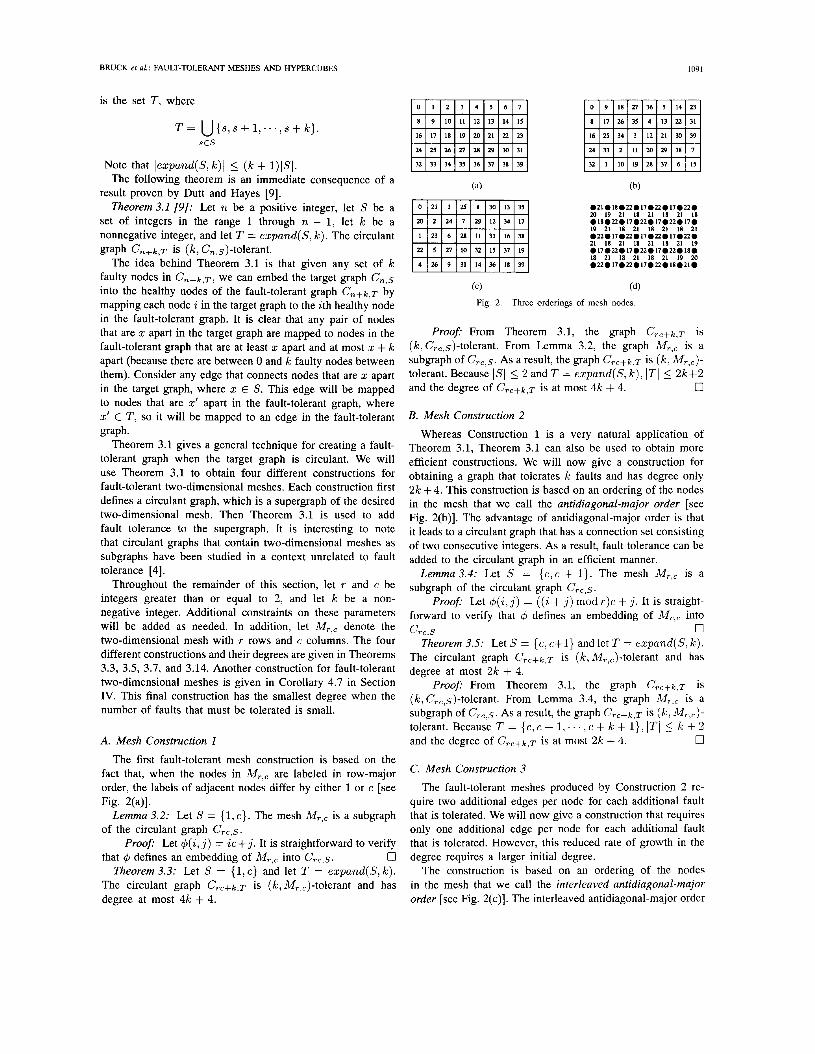
Fig. 3. Three orderings of mesh nodes for the mesh construction 4: (a) T is odd, (b) T mod4 = 0. and (c) T mod4 = 2 .

distinct values. From Lemma 3.9, r and ( r - 1)/2 are relatively prime, so for any integers x and x’, if f(x) = f ( d ) it follows that x mod r = x’ mod r. Let ( 2 , j ) and (i ‘ , j ’ ) be any nodes in Mr,c. Note that f ( i + j ) c and j ( i ’ + j ’ ) c are multiples of c, and that j E [e] and j ‘ E [c]. Therefore, if $ ( i , j ) = 4( i ’ , j ’ ) , it follows that j = j ’ , which implies that f ( i + j ) = f ( i ’ + j ’ ) , so i m o d r = i ’modr and i = i ’ .

We will now show that 4 maps edges in MT,c to edges in CTC,s. We will show this by proving that for any integers i and j , i) I4(i + 1 , j ) - d ( i , j ) l E close(S,rc), and ii) I4(i,j + 1) - b( i , j ) I E close(S,rc). Let s = ( r - 1)c/2 and let s’ = ( r + l)c/2, and note that close(S,rc) = {s,s + 1,s’ 1 l,s’}. In addition, note that for any integer x , f ( x + 1) - f(x) equals either ( r - 1)/2 or - ( r + 1)/2. Therefore, I4(i + 1 , j ) - 4( i , j ) l = I f ( i + j + 1) - f ( i + j ) l c , which equals either s or s’, and property i holds. Let 4 ( i , j ) = y. Clearly, $ ( i , j + 1) = 4(i + 1 , j ) + 1, which equals either y + s + 1 or y - s’ + 1, so property ii holds as well. As a

0 Lemma3.11: Let r m o d 4 = 0 and let S = {(r /2 -

l )c , ( r /2 - 1)c + l}. The mesh Mr,c is a subgraph of the circulant graph CrC,s.

Proof: Let f ( i ) = ( ( r /2 - 1 ) i ) m o d r and let qh(i,j) = f ( i + j ) c + j . The proof is analogous to that of Lemma 3.10

0 Lemma3.12: Let r m o d 4 = 2 and let S = { ( r / 2 -

2)c, ( r /2 - 2)c + 1). The mesh Mr,c is a subgraph of the circulant graph CTc,s.

Proof: Let f ( i ) = ( ( r / 2 - 2 ) i ) m o d r and let 4 ( i , j ) = f ( i + j ) c + j . The proof is analogous to that of Lemma 3.10

0 Fig. 3 shows examples of the mapping 4 for three meshes,

representing the cases of Lemmas 3.10 through 3.12, respectively.

Definition: Let n , s , and x be integers where 0 5 s < Ln/2] and 0 5 x I s, and let S = {s - x, s - z + 1 , . . . , s}. Then gap(S ,n ) = n - 1 - 2s.

Intuitively, gap( S, n) is the length of the “gap” between the two consecutive groups of offsets in close(S, n ) . For instance, if S = {5,6},close(S,16) = {5,6,10,11} and gap(S , 16) = 3. The following lemma is similar to one proven by Dutt and Hayes [9].

result, 4 is an embedding of Mr,c into CTC,s.

and will not be repeated here.

and will not be repeated here.

Lemma 3.13: Let n, s, and x be integers where 0 5 s < Ln/2J and 0 I z I s , let S = {s - 5,s - z + l , . . . , s } and let T = expand(S,k). The circulant graph Cn+k,T has degree at most

d = { 2IC + 2 ( S ( , if k- I g a p ( S , n ) , if IC > gap(S , n). k + 21SI + gap(S , n ) ,

Proof: The fact that d 5 2k + 21S( follows immediately from the definitions of expansion and closure. Now consider the case where IC > g a p ( S , n ) . Note that T = {s - x, s - x + 1, . . . , s + I C } so we will compare the values of s + IC and n + IC - (s + I C ) = n - s to see if there is a gap between the two groups of offsets in close(T,n + I C ) . Note that (n - s) - (s + k ) = n - 2s - I C , which is less than n - 2s - (n - 1 - 2.9) = 1 because k > g a p ( S , n ) = n - 1 - 2s. Therefore, there is no gap between the two groups of offsets in close(T,n + I C ) , so close(T,n + IC) = {s - 2 , s -x+ 1,. . . , n+ k - (s -x)} and Iclose(T, n+lc)l = n + IC - (s - x) - (s - x - 1) = n + IC - 2s + 22 + 1. Since IC + 21SI + gap(S , n) = IC + 2(x + 1) + n - 1 - 2s, we have

0 JcZose(T, n + I C ) \ = IC + 215’1 + g a p ( S , n). Theorem 3.14: Let

{(i - l )c , (i - l )c+’l} if r mod 4 = 0,

{ (i - 2)c, (f - 2). + 1} if r mod 4 = 2,

and let T = expand(S, k ) . Then the circulant graph Crc+k,T

is ( I C , M,,,)-tolerant and has degree at most

d(k, r, c) =

’ 2k + 4, e + I C + 1, 2IC + 4, 2c + k + 1, 21C + 4,

, 4c + k + 1,

r is odd and k 5 c - 3 , r is odd and IC > c - 3, r mod 4 = 0 and IC 5 2c - 3 , r mod 4 = 0 and IC > 2c - 3, r mod 4 = 2 and IC I 4c - 3, r mod 4 = 2 and IC > 4c - 3.

Proof: From Theorem 3.1, the graph Crc+k,T is ( I C , C,,,s)-tolerant. From Lemmas 3.10 to 3.12, the graph is a subgraph of CrC,s. Thus, the graph Crc+k,T is ( I C , tolerant. The degree follows directly from Lemma 3.13 and the fact that gap(S, r e ) = c - 3 if r is odd, 2c - 3 if r mod 4 = 0, and 4c - 3 if r m o d 4 = 2. 0

Note that if the numbers 0,1, . . . , rc - 1 are assigned to meshes in the diagonal manner instead of the antidiagonal manner, then the new gap(S , re) is greater than the original g a p ( S , rc) by 2.

IV. DIAGONAL GRAPHS In Section 111, we studied the family of circulant graphs.

Another important class of graphs consists of what we call “diagonal graphs.” In this section we will show that diagonal graphs can be used to create fault-tolerant d-dimensional meshes and hypercubes with small degree. We will also present efficient implementations for many of these fault- tolerant graphs. The definition of diagonal graphs and a general technique for adding fault tolerance to diagonal graphs are given next.

IEEE TRANSACTIONS ON COMPUTERS, VOL. 42, NO. 9. SEPTEMBER 1993

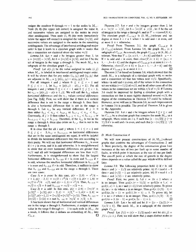
Fig. 4.

B

Diagonal graph with 16 nodes and offsets 1 and 4.

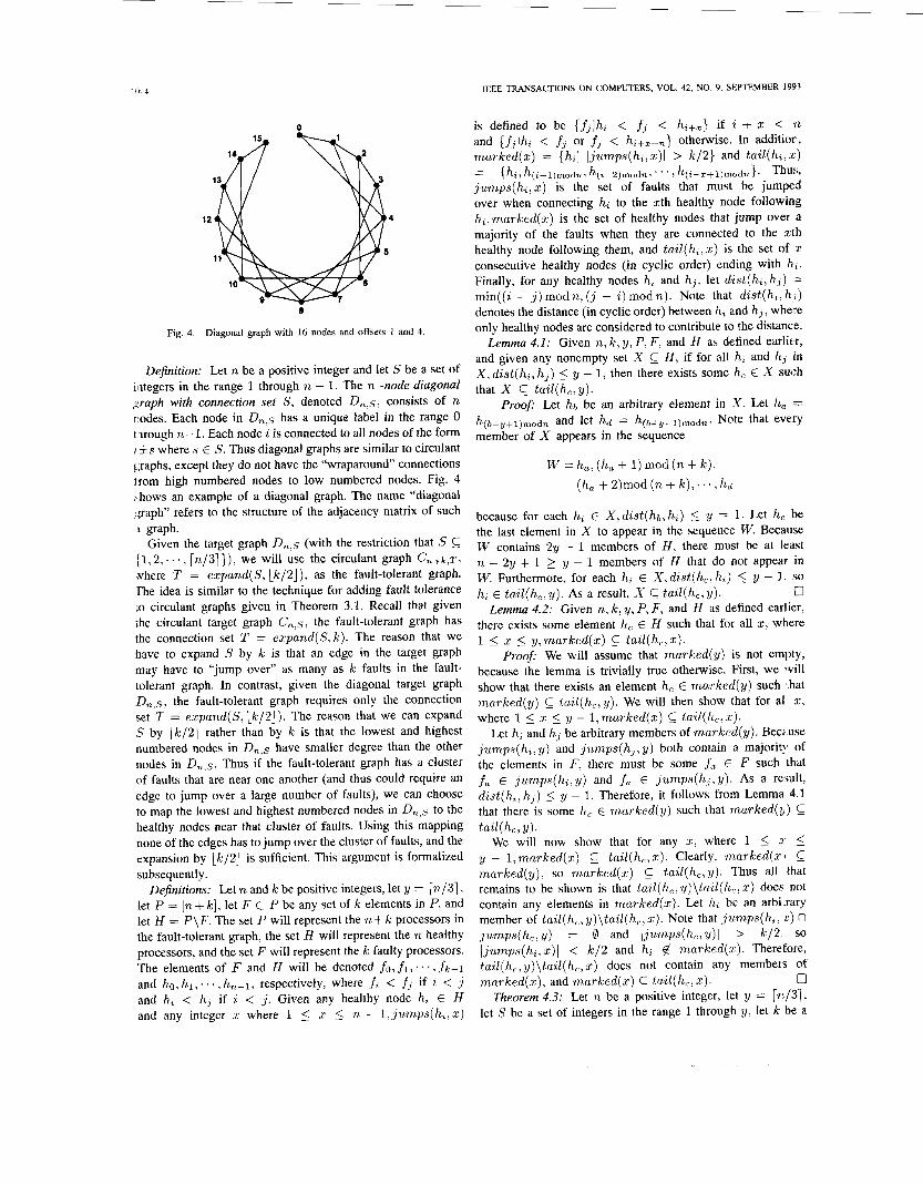
Definition: Let n be a positive integer and let S be a set of iiitegers in the range 1 through n - 1. The n -node diagonal graph with connection set S, denoted Dn,s, consists of n rodes. Each node in Dn,s has a unique label in the range 0 t irough n- 1. Each node z is connected to all nodes of the form I f s where s E S. Thus diagonal graphs are similar to circulant t,raphs, except they do not have the “wraparound” connections from high numbered nodes to low numbered nodes, Fig. 4 chows an example of a diagonal graph. The name “diagonal ~raph” refers to the structure of the adjacency matrix of such L graph.

Given the target graph Dn,s (with the restriction that S C [ 1 , 2 , . . . , [n/31}), we will use the circulant graph C n + k , ~ ,

where T = ezpand(S , Lk/2]), as the fault-tolerant graph. The idea is similar to the technique for adding fault tolerance LO circulant graphs given in Theorem 3.1. Recall that given the circulant target graph C,,s, the fault-tolerant graph has the connection set T = expand(S , k ) . The reason that we have to expand S by k is that an edge in the target graph may have to “jump over” as many as k faults in the fault- tolerant graph. In contrast, given the diagonal target graph D,,s , the fault-tolerant graph requires only the connection set T = ezpand(S , Lk /2]) . The reason that we can expand S by Lk/2] rather than by k is that the lowest and highest numbered nodes in D,,s have smaller degree than the other nodes in D,,s. Thus if the fault-tolerant graph has a cluster of faults that are near one another (and thus could require an edge to jump over a large number of faults), we can choose to map the lowest and highest numbered nodes in D,,s to the healthy nodes near that cluster of faults. Using this mapping none of the edges has to jump over the cluster of faults, and the expansion by Lk/2J is sufficient. This argument is formalized subsequently.

Definitions: Let n and k be positive integers, let y = [n/31, let P = [n + k ] , let F c P be any set of k elements in P, and let H = P\F. The set P will represent the n + k processors in the fault-tolerant graph, the set H will represent the n healthy processors, and the set F will represent the k faulty processors. The elements of F and H will be denoted f o , f l , . . . , fk-1

and ho, h l , . . . , hn-l, respectively, where f z < f, if z < 1 and h, < h, if a < 3. Given any healthy node h, E H and any integer z where 1 5 T 5 n - l , jumps(h , ,x )

is defined to be {fjlhi < fj < hi+%} if i + x < 11

and {fjlhi < f, or fj < hi+l-n} otherwise. In additior, marked(%) = (hi1 Ijumps(hi,z)( > k / 2 } and t a i l ( h i , x )

jumps(hi,z) is the set of faults that must be jumped over when connecting hi to the xth healthy node following h i , m a r k e d ( x ) is the set of healthy nodes that jump over a majority of the faults when they are connected to the zth healthy node following them, and tail(h;,x) is the set of x consecutive healthy nodes (in cyclic order) ending with h; . Finally, for any healthy nodes hi and hi , let dist(hi, h j ) = min((i - j ) m o d n , ( j - i) m o d n ) . Note that dist(hi, h,;) denotes the distance (in cyclic order) between h; and hj, whe:e only healthy nodes are considered to contribute to the distance.

Lemma 4.1: Given n, k , y, P, F , and H as defined earlier, and given any nonempty set X H , if for all hi and hj in X , dist(hi, h j ) 5 y - 1, then there exists some h, E X such that X 5 ta i l (h , ,y ) .

Proof: Let hb be an arbitrary element in x. Let ha = h(b-y+l)mo& and let h d = h(b+y- l )modn. Note that every member of X appears in the sequence

= {hi, h ( i - l ) m o d n , h(i--2)modn, ’ ‘ . > h ( i - z + l ) m o d n } . Thuh

W = ha, (ha + 1) mod (n + k ) . (ha + 2)mod (n + k ) , . . . , hd

because for each hi E X,dis t (hb, hi) 5 y = 1. Let h, be the last element in X to appear in the sequence W. Because W contains 2y - 1 members of H , there must be at least n - 2y + 1 2 y - 1 members of H that do not appear in W. Furthermore, for each hi E X , dist(h,, hi) 5 y - I, SO

0 Lemma 4.2: Given n, k , y , P, F, and H as defined earlier,

there exists some element h, E H such that for all z, where 1 5 3: 5 y , m a r k e d ( x ) C tail(h,,z).

Proof: We will assume that marked(:y) is not empty, because the lemma is trivially true otherwise. First, we will show that there exists an element h, E m a r k e d ( y ) such ‘.hat m a r k e d ( y ) C tai l (h , ,y) . We will then show that for a1 z, where 1 5 x 5 y - l ,marked(x) C tail(h,,.c).

Let hi and hj be arbitrary members of marked(y ) . Bec2use jumps(hi, y ) and jumps(hj, y ) both contain a majorit!’ of the elements in F, there must be some f a E F such that fa E jumps(h;,y) and fa E jumps(hj,y). As a result, dist(h,, h j ) 5 y - 1. Therefore, it follows from Lemma 4.1 that there is some h, E m a r k e d ( y ) such that marked(%) C

We will now show that for any x, where 1 5 3. 5 y - I , m a r k e d ( z ) C tail(h,,z). Clearly, marked(x1 C m a r k e d ( y ) , so m a r k e d ( x ) C ta i l (h , ,y ) . Thus all that remains to be shown is that tail(h,, y)\tclil(h,, x) does not contain any elements in marked(%). Let hi be an arbi:rary member of tail(h,, y)\tail(h,,z). Note that .jumps(hi, E ) n j u m p s ( h , , y ) = 0 and Ijumps(h,,,y)l > k / 2 . so Jjumps(hi,z)) < k / 2 and hi 6 marked( z ) . Therefore, tail(& y)\tail(h,,z) does not contain any members of

0 Theorem 4.3: Let n be a positive integer, let y = [?!/31 ,

let S be a set of integers in the range 1 through y , let k be a

h; E tail(h,, y) . As a result, X C taiZ(h,, y).

tail( h,, y ) .

marked(x ) , and marked(z) C tail(h,,x).

1095 BRUCK et al.: FAULT-TOLERANT MESHES AND HYPERCUBES

positive integer, and let T = expan,d(S: [k: /2] ) . The circulant graph C,+k)T is ( k , D,,s)-tolerant.

Proof: We will show the existence of an embedding d, that maps the nodes of DTL,s to the healthy nodes in C,{+~ ,T . Let P, F. and H be as defined earlier, with P representing the nodes in C,+~,T> F representing an arbitrary set of k: faulty nodes, and H representing the remaining 71 healthy nodes. From Lemma 4.2, there exists a node h,,. E H such that for all x , where 1 5 z 5 y ,mm-ked( . r ) C tail(h,,.:e). Let h, = (h , + 1) mod ( n + k ) . Define the function d, that maps from [n,] to [n+k] such that for any ,i E [n,]. 4 ( i ) = h ( z + z ) m o d n .

We will show that 4 is an embedding of Dn..y into the healthy nodes in Cn+k,T. It is clear that for any node i in D,,s, 4( i ) is a healthy node in C n + k . ~ . In addition, it is clear that for any distinct nodes i and j in Dn,s . $( i ) # 4(:j). Thus all that remains to be shown is that for any edge ( i . j ) in D,,s. (d( i ) ,d , ( . j ) ) is an edge in CT,+k.T. Every edge in Dn.s is of the form (a: a + .T) , where (I E [n - x] and :r E S. We will show that (d (u ) . d ( a + x)) is an edge in C,,+~.,T. Note that d ( a ) = h ( z + a ) m o d n , and because a E [n, - . T I . 4 ( a ) tail(h,, x ) . However, h,, was selected so that mmrked(:r:) C tail(h,,n:), so it follows that Ijumps(q5(n),z)/ 5 [ k / 2 ] and 5 + Ijumps(d(a), x)I E T. Therefore, ( d ( a ) . d(o, + , E ) ) is an edge in Cn+k,T.

(b) A. d-Dimensional Meshes and Hypercubes The previous theorem on diagonal graphs can be used to

construct efficient fault-tolerant d-dimensional meshes and

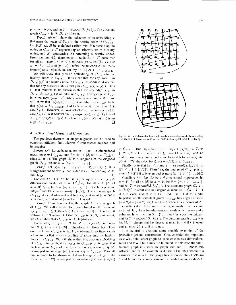
Fig. S . (a) A 6 x 6 one-fault-tolerant two-dimensional mesh. (b) New labeling of the fault-tolerant mesh when the node with original label 13 is faulty.

hypercubes. Lemma 4.4: Let M be an n,o x 721 x . . . x njrl-l d-dimensional

mesh, let TI, = II::; n,t. and for all 1 E [d] let s i = IItzi 71j

(thus so = 1). The graph M is a subgraph of the diagonal graph Dn,s, where s = { s o . 9 1 . . . . . sd - 1) .

straightforward to verify that q5 defines an embedding of M

Theorem 4.5: Let M be an no x n,1 x . . . x fr1,1-1 d- dimensional mesh, let n, = IIfzi n,i, for all i E [ d ] let s, = IIgzi n3, let S = {sg. s l , . . . , s d - l } . let k be a positive integer, and let T = ezpnn,d(S, [ k / 2 ] ) . The circulant graph C,+~,T is ( I C , M)-tolerant and has degree at most ( k + 2)d if k is even, and at most ( k + 1)d if k is odd.

Proof: From Lemma 4.4, the graph M is a subgraph of D,,s. We will consider two cases based on the value of n d - 1 . If n d - 1 2 3. then S C { 1 , 2 : . . . , [ n / 3 ] } . Therefore, it follows from Theorem 4.3 that C,+~.T is ( k . D,,.s)-tolerant, which implies that C,+~,T is ( k , AI)-tolerant.

Conversely, if nd-1 = 2 let S' = S\{n,/2} and note that S' C { 1 , 2 . . . . ~ Ln/3)}. Therefore, it follows from The- orem 4.3 that C,+~.T is ( k . D,,sf)-tolerant, so there exists a function 4 that is an embedding of D,,s, into the healthy nodes in C,+,+,T. We will show that q5 is also an embedding of Dn,s into the healthy nodes in C n + k , ~ . It is clear that each edge in D,,s of the form ( i , i + x). where :E E S'. is mapped to an edge (4(i),d,(i + x ) ) in C,,+~.T. Thus all that remains to be shown is that each edge in Dn,s of the form (zli + n/2) is mapped to an edge (4(6).4(i + n, /2) )

Proof: Let 4(n0.a813.. . .ad-l) = E,=, d - 1 ( u i ) ( s , ) . It is

into Dn>s. 0

in C,,+~.T. But {n/2,71,/2 + l , . . . , n , / 2 + L k / 2 ] } C T , so {n/2.71/2 + l , . . . , r 1 , / 2 + k } C closc(T,n + k), and no matter how many faulty nodes are located between d,(i) and 4(1 + n/2) , the edge ( d ( i ) , cj(i + n / 2 ) ) is in C n + k , ~ .

Finally, note that IS1 5 d and T = e:rpand(S, L k / 2 ] ) , so (TI 5 d ( 1 + [k/Zj) . Therefore, the degree of Cn+k,T is at most ( k + 2 ) d if k is even and at most ( k + 1)d if k is odd.0

Corollary 4.6: Let Q ( 1 be a d-dimensional hypercube, let n = 2 ' , f o r a l l i ~ [d] I e t s , = 2 ' , ~ e t S = { s o , . ~ 1 . ~ ~ ~ , s ~ - - l } , and let T = cxpand(S, [ k / 2 J ) . The circulant graph C n + k . ~

is ( k . Qd)-tolerant and has degree at most ( k + 2 ) d - k - 1 if k is even, and at most ( k + l ) d - k + 1 if k is odd. In particular, the circulant graph C,,,,. has degree at most ( k + 2)d - ( k + 2 ) log k + 2k - 3 when k: is a power of 2.

Corollary 4.7: Let r and c be integers greater than or equal to 2, let M r ~ , be a two-dimensional mesh with T rows and c columns, let n = T C , let S = { 1, c}. let k be a positive integer, and let T = ezpn,71,d(S. [ k / 2 ) ) . The circulant graph C,+~,T is ( k . M?,,)-tolerant and has degree at most 2k + 4 if k is even, and at most 2k + 2 if k: is odd.

I t is helpful to examine some specific examples of the preceding general construction. First, consider the important case where the target graph A4 is an m x m two-dimensional mesh and k = 1 fault must be tolerated. In this case the fault- tolerant graph is a circulant graph with m2 + 1 nodes and offsets 1 and m,. An example is shown in Fig. 5(a), where it is assumed that m = 6. The graph has 37 nodes, the offsets are 1 and 6, and the connections are calculated using modulo-37

IEEE TRANSACTIONS ON COMPUTERS, VOL. 42, NO. 9. SEPTEMBER 1993

I I I I I I I I I t

a

I I I I I I I I I

b c d e i I

I I I I

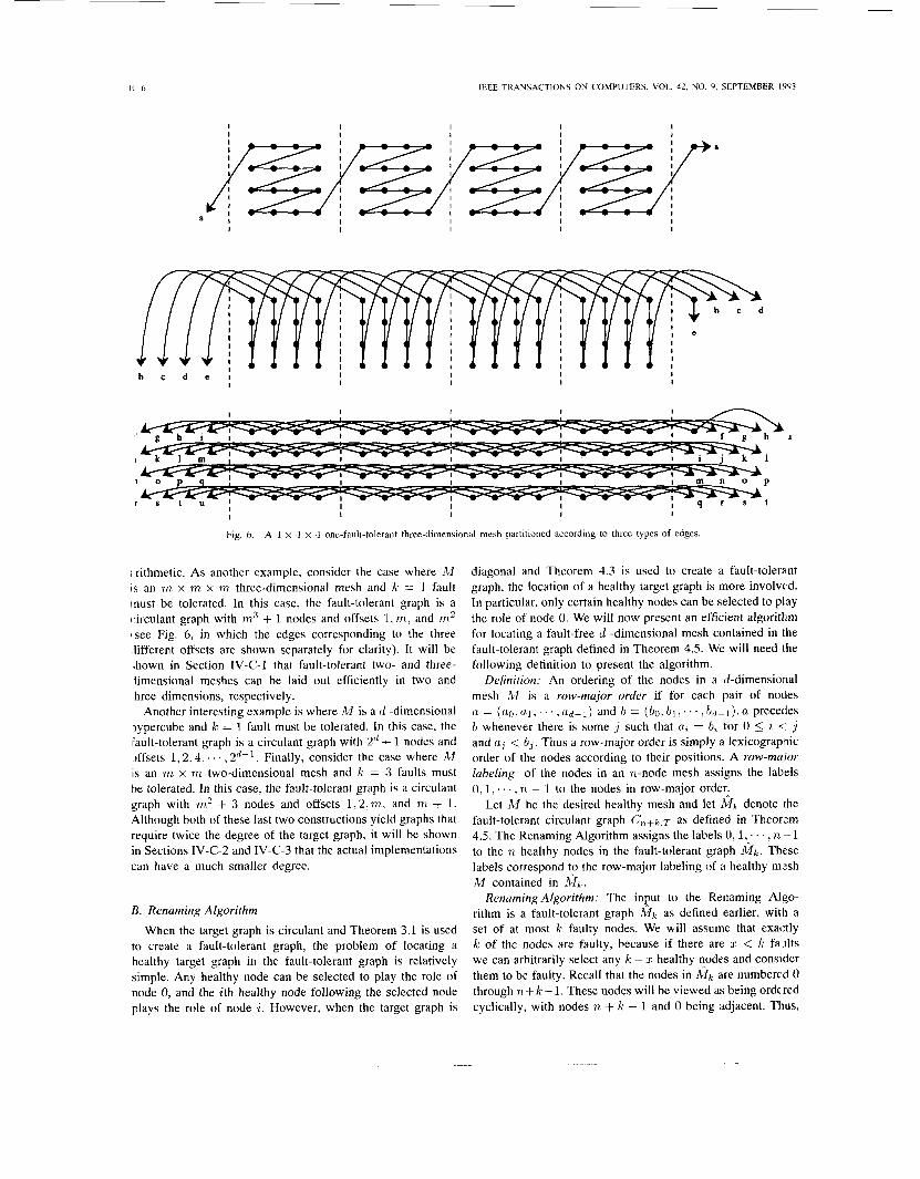
Fig. 6. A 4 x 4 x 4 one-fault-tolerant three-dimensional mesh partitioned according to three types of edges.

; rithmetic. As another example, consider the case where M i s an m x m x r n three-dimensional mesh and k = 1 fault inust be tolerated. In this case, the fault-tolerant graph is a ~irculant graph with m3 + 1 nodes and offsets l . m , and m 2 #see Fig. 6, in which the edges corresponding to the three iifferent offsets are shown separately for clarity). It will be ,hown in Section IV-C-1 that fault-tolerant two- and three- iimensional meshes can be laid out efficiently in two and hree dimensions, respectively.

Another interesting example is where M is a d -dimensional iypercube and k = 1 fault must be tolerated. In this case, the fault-tolerant graph is a circulant graph with 2" + 1 nodes and 3ffsets 1 ,2 .4 , . . . .2"-l. Finally, consider the case where A4 IS an m x ni two-dimensional mesh and k = 3 faults must be tolerated. In this case, the fault-tolerant graph is a circulant graph with m2 + 3 nodes and offsets 1 ,2 .m. and m + 1. Although both of these last two constructions yield graphs that require twice the degree of the target graph, it will be shown in Sections IV-C-2 and IV-C-3 that the actual implementations can have a much smaller degree.

B. Renaming Algorithm When the target graph is circulant and Theorem 3.1 is used

to create a fault-tolerant graph, the problem of locating a healthy target graph in the fault-tolerant graph is relatively simple. Any healthy node can be selected to play the role of node 0, and the ith healthy node following the selected node plays the role of node i . However, when the target graph is

diagonal and Theorem 4.3 is used to create a fault-tolerant graph, the location of a healthy target graph is more involved. In particular, only certain healthy nodes can be selected to play the role of node 0. We will now present an efficient algorithm for locating a fault-free d -dimensional mesh contained in the fault-tolerant graph defined in Theorem 4.5. We will need the following definition to present the algorithm.

Definition: An ordering of the nodes in a d-dimensional mesh A4 is a row-major order if for each pair of nodes n = (fig. u1. . . . , n d - 1 ) and b = (bo. b l , . . . , h d - l ) , u precedes b whenever there is some ,J' such that ai = hi for 0 5 i <: j and u j < b, . Thus a row-major order is simply a lexicographic order of the nodes according to their positions. A row-maior labeling of the nodes in an n,-node mesh assigns the labels 0, I , . . . , n - 1 to the nodes in row-major order:

Let M be the desired healthy mesh and let Mk denote the fault-tolerant circulant graph Cn+k,T as defined in Theorem 4.5. The Renaming Algorithm assigns the labels O , l , - . . . , n - 1 to the 71, healthy nodes in the fault-tolerant graph h f k . These labels correspond to the row-major labeling of a healthy mssh M contained in Mk.

Renaming Algorithm: The input to the Renaming Ngo- rithm is a fault-tolerant graph Mk as defined earlier, with a set of at most k faulty nodes. We will assume that exactly k of the nodes are faulty, because if there are .T < k: failts we can arbitrarily select any IC - 5 healthy nodes and consider them to be faulty. Recall that the nodes in h.r, are numbered 0 through n + k: - 1. These nodes will be viewed as being ordc red cyclically, with nodes n, + k - 1 and 0 being adjacent. Thus,

BRUCK et al .: FAULT-TOLERANT MESHES AND HYPERCUBES IO9 7

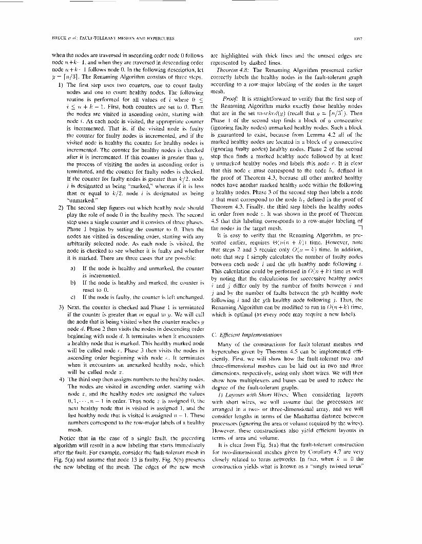
when the nodes are traversed in ascending order node 0 follows node n+k- l , and when they are traversed in descending order node n + k - 1 follows node 0. In the following description, let y = [n/31. The Renaming Algorithm consists of three steps.

The first step uses two counters, one to count faulty nodes and one to count healthy nodes. The following routine is performed for all values of ‘i where 0 5 i 5 71 + k - 1. First, both counters are set to 0. Then the nodes are visited in ascending order, starting with node 1;. As each node is visited, the appropriate counter is incremented. That is, if the visited node is faulty the counter for faulty nodes is incremented, and if the visited node is healthy the counter for healthy nodes is incremented. The counter for healthy nodes is checked after it is incremented. If this counter is greater than y. the process of visiting the nodes in ascending order is terminated, and the counter for faulty nodes is checked. If the counter for faulty nodes is greater than k / 2 . node z is designated as being “marked,” whereas if i t is less than or equal to k / 2 . node i is designated as being “unmarked.” The second step figures out which healthy node should play the role of node 0 in the healthy mesh. The second step uses a single counter and i t consists of three phases. Phase 1 begins by setting the counter to 0. Then the nodes are visited in descending order, starting with any arbitrarily selected node. As each node is visited, the node is checked to see whether it is faulty and whether it is marked. There are three cases that are possible:

If the node is healthy and unmarked, the counter is incremented. If the node is healthy and marked, the counter is reset to 0. If the node is faulty, the counter is left unchanged.

Next, the counter is checked and Phase 1 is terminated if the counter is greater than or equal to y. We will call the node that is being visited when the counter reaches node d. Phase 2 then visits the nodes in descending order beginning with node d. It terminates when i t encounters a healthy node that is marked. This healthy marked node will be called node c. Phase 3 then visits the nodes in ascending order beginning with node c. I t terminates when it encounters an unmarked healthy node, which will be called node z . The third step then assigns numbers to the healthy nodes. The nodes are visited in ascending order, starting with node z , and the healthy nodes are assigned the values 0.1, . . ,TI , - 1 in order. Thus node z is assigned 0, the next healthy node that is visited is assigned 1, and the last healthy node that is visited is assigned 71 - 1. These numbers correspond to the row-major labels of a healthy mesh.

a)

b)

c)

Notice that in the case of a single fault, the preceding algorithm will result in a new labeling that starts immediately after the fault. For example, consider the fault-tolerant mesh in Fig. 5(a) and assume that node 13 is faulty. Fig. 5(b) presents the new labeling of the mesh. The edges of the new mesh

are highlighted with thick lines and the unused edges are represented by dashed lines.

Theorem 4.8: The Renaming Algorithm presented earlier correctly labels the healthy nodes in the fault-tolerant graph according to a row-major labeling of the nodes in the target mesh.

Proof: It is straightforward to verify that the first step of the Renaming Algorithm marks exactly those healthy nodes that are in the set ~ r r ~ m - k c d ( g ) (recall that = [ ~ t , / 3 1 ) . Then Phase 1 of the second step finds a block of y consecutive (ignoring faulty nodes) unmarked healthy nodes. Such a block is guaranteed to exist, because from Lemma 4.2 all of the marked healthy nodes are located in a block of g consecutive (ignoring faulty nodes) healthy nodes. Phase 2 of the second step then finds a marked healthy node followed by at least y unmarked healthy nodes and labels this node c. It is clear that this node c must correspond to thc node h,. defined in the proof of Theorem 4.3, because all other marked healthy nodes have another marked healthy node within the following y healthy nodes. Phase 3 of the second step then labels a node z that must correspond to the node h Z defined in the proof of Theorem 4.3. Finally, the third step labels the healthy nodes in order from node z . It was shown in the proof of Theorem 4.5 that this labeling corresponds to a row-major labeling of

0 I t is easy to verify that the Renaming Algorithm, as pre-

scnted earlier, requires (-)(n(n + X:)) time. However, note that steps 2 and 3 require only O(r/ + X ) time. In addition, note that step 1 simply calculates the number of faulty nodes between each node i and the yth healthy node following I .

This calculation could be performed in O ( n + k ) time as well by noting that the calculations for successive healthy nodes i and , j differ only by the number of faults between i and , j and by the number of faults between the yth healthy node following i and the yth healthy node following , j . Thus, the Renaming Algorithm can be modified to run in O ( 7 1 - t k ) time, which is optimal (as every node may require a new label).

the nodes in the target mesh.

C. Eficient Implementations

Many of the constructions for fault-tolerant meshes and hypercubes given by Theorem 4.5 can be implemented efficiently. First, we will show how the fault-tolerant two- and three-dimensional meshes can be laid out in two and three dimensions, respectively, using only short wires. We will then show how multiplexers and buses can be used to reduce the degree of the fault-tolerant graphs.

1) Layouts with Short Wires: When considering layouts with short wires, we will assume that the processors are arranged in a two- or three-dimensional array, and we will consider lengths in terms of the Manhattan distance between processors (ignoring the area or volume required by the wires). However, these constructions also yield efficient layouts in terms of area and volume.

It is clear from Fig. S(a) that the fault-tolerant construction for two-dimensional meshes given by Corollary 4.7 are very closely related to torus networks. In fact, when A. = 0 the construction yields what is known as a “singly twisted torus”

IEEE TRANSACTIONS ON COMPUTERS, VOL. 42, NO. ' 2 , SEPTEMBER 19'13

P 1 2 3 4 5 6 7

(b)

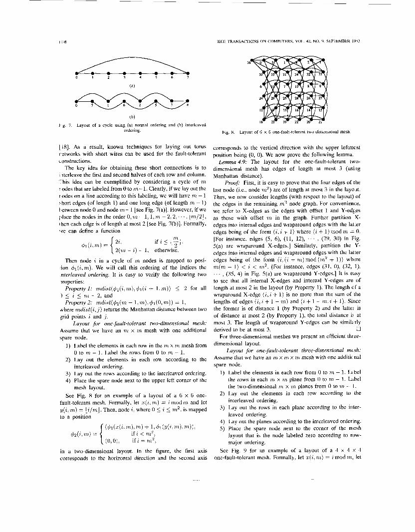
1. g. 7. Layout of a cycle using (a) normal ordering and (b) interleaved

3

Fig. 8. Layout of 6 x 6 one-fault-tolerant two-dimensional mesh. ordering.

1181. As a result, known techniques for laying out torus retworks with short wires can be used for the fault-tolerant constructions.

The key idea for obtaining these short connections is to I iterleave the first and second halves of each row and column. ':'his idea can be exemplified by considering a cycle of m I odes that are labeled from 0 to m-I . Clearly, if we lay out the I odes on a line according to this labeling, we will have m - 1 5hort edges (of length 1) and one long edge (of length m - 1) t letween node 0 and node m- 1 [see Fig. 7(a)]. However, if we [dace the nodes in the order 0, m - 1, I , m - 2 ,2 , . . . , Im/2], 1 hen each edge is of length at most 2 [see Fig. 7(b)]. Formally, rve can define a function

m 2 { i i m - i ) - 1, otherwise.

if i 5 1-1, m) =

Then node i in a cycle of m nodes is mapped to posi- lion &( i , m). We will call this ordering of the indices the .nterleaved ordering. It is easy to verify the following two xoperties:

Property I : mdist(q51(i,m),q51(i + 1 , m ) ) 5 2 for all 1 5 i 5 m - 2 , a n d

Property 2: mdist(&(m - 1, m), &(0, m) ) = 1, where mdist(i , j ) returns the Manhattan distance between two grid points i and j.

Layout for one-fault-tolerant two-dimensional mesh: Assume that we have an m x m mesh with one additional spare node.

I) Label the elements in each row in the m x m mesh from

2) Lay out the elements in each row according to the

3) Lay out the rows according to the interleaved ordering. 4) Place the spare node next to the upper left corner of the

See Fig. 8 for an example of a layout of a 6 x 6 one- fault-tolerant mesh. Formally, let x ( i , 772) = i mod m and let y ( i , m) = li/m,J. Then, node z, where 0 5 i 5 m 2 , is mapped to a position

0 to m - 1. Label the rows from 0 to m - 1.

interleaved ordering.

mesh layout.

( 4 1 ( 4 i , m ) , m ) + L d l ( Y ( i , m ) , m ) ) , if i < m2, { (o ,o) , if i = m 2 ,

42(i,m) =

in ii two-dimensional layout. In the figure, the first axis corresponds to the horizontal direction and the second axis

corresponds to the vertical direction with the upper leftmclst position being (0, 0). We now prove the following lemma.

Lemma 4.9: The layout for the one-fault-tolerant two- dimensional mesh has edges of length at most 3 (using Manhattan distance).

Proof: First, it is easy to prove that the four edges of the last node (Le., node m2) are of length at most 3 in the layoit. Thus, we now consider lengths (with respect to the layout) of the edges in the remaining m2 node graph. For convenience, we refer to X-edges as the edges with offset 1 and Y-edges as those with offset m in the graph. Further partition Y- edges into internal edges and wraparound edges with the latter edges being of the form (2, z + 1) where (i + 1) mod m = 0. [For instance, edges (5, 6), (11, 12), . . . , (29, 30) in Fig. 5(a) are wraparound X-edges.] Similarly, partition the Y- edges into internal edges and wraparound edges with the latter edges being of the form ( A , ( 7 + m) mod (7n2 + 1)) where m(m - 1) < z < m2. [For instance, edges (31, O), (32, I), . . . , (35, 4) in Fig. 5(a) are wraparound Y-edges.] It is easy to see that all internal X-edges and internal Y-edges are of length at most 2 in the layout (by Property 1). The length cf a wraparound X-edge (z , z + 1) is no more than the sum of the lengths of edges (z,z + 1 - m) and (z + I - m,z + 1). Since the former is of distance 1 (by Property 2) and the lattei is of distance at most 2 (by Property I), the total distance i: at most 3. The length of wraparound Y-edges can be simikrly derived to be at most 3. 0

For three-dimensional meshes we present an efficient three- dimensional layout.

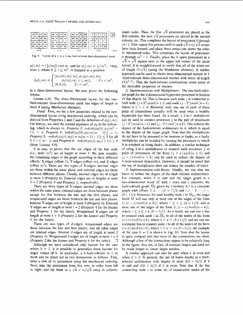
Layout for one-fault-tolerunt three-dimensional mesh: Assume that we have an m x m x m mesh with one additicnal spare node.

1) Label the elements in each row from 0 to m - 1. L bel the rows in each m x m plane from 0 to m - 1. Label the two-dimensional m x m planes from 0 to m - 1.

2) Lay out the elements in each row according to the interleaved ordering.

3) Lay out the rows in each plane according to the interleaved ordering.

4) Lay out the planes according to the interleaved ordering. 5 ) Place the spare node next to the corner of the mesh

layout that is the node labeled zero according to row- major ordering.

See Fig. 9 for an example of a layout of a 4 x 4 x 4 one-fault-tolerant mesh. Formally, let ~ ( i , 711) = z mod m, let

BRUCK et ai.: FAULT-TOLERANT MESHES AND HYPERCUBES 1099

r = 4 r = 3 ’ r = 2 r = l I z = o

Fig. 9. Layout of 4 x 4 x 4 one-fault-tolerant three-dimensional mesh.

y(i, m) = (Li/m]) modm, and let z ( i , m) = Li/m2]. Then, node i , where 0 5 a 5 m3, is mapped to a position

( 4 l ( Z ( i : m): m): 41(di, m), m), 4 l ( z ( i , m) + 1, m)). if i < m3, { ( O , O , O ) , if i = m3,

$3(i1m) =

in a three-dimensional layout. We now prove the following lemma.

Lemma 4.10: The three-dimensional layout for the one- fault-tolerant three-dimensional mesh has edges of length at most 4 (using Manhattan distance).

Proof: First, we list a few properties related to the two- dimensional layout using interleaved ordering, which can be derived from Properties 1 and 2 and the definition of 4 2 ( s i ~ m). For brevity, we omit the second argument of 42 in the following, which is always m. Property 3: mdist(42(0), 42(m2 - 1)) = 2; Property 4: mdist(42(0),42(m(m - 1))) = 1; Property 5: mdist(4z(i), 42(i + m(m - 1) + 1)) 5 3 for all 0 5 i 5 m - 1; and Property 6: mdist(42(i), 42(i + 1)) I 3 (from Lemma 4.9).

It is easy to prove that the six edges of the last node (Le., node m3) are of length at most 4. We now consider the remaining edges in the graph according to three different offsets: X-edges (offset l) , Y-edges (offset m), and Z-edges (offset m2). There are two types of X-edges: internal edges are those within the same plane, and external edges are those between different planes. Clearly, internal edges are of length at most 3 (Property 6). External edges are of lengths at most 2 + 2 (Property 3 and Property 1, respectively).

There are three types of Y-edges: internal edges are those within the same plane, external edges are those between planes except for that between the last and the first planes, and wraparound edges are those between the last and first planes. Internal Y-edges are of length at most 3 (Property 6). External Y-edges are of length at most 1 + 2 (Property 4 for the former and Property 1 for the latter). Wraparound Y-edges are of length at most 1 + 3 (Property 2 for the former and Property 5 for the latter).

There are two types of Z-edges: wraparound edges are those between the last and first planes, and all other edges are internal edges. Internal Z-edges are of length at most 2 (Property 1). Wraparound Z-edges are of length at most 1 + 3 (Property 2 for the former and Property 6 for the latter). 0

Although we have considered only layouts for the case where k = 1, it is possible to generalize these layouts for larger values of k . In particular, a k-fault-tolerant m x m mesh can be layed out in two dimensions as follows. First, label a row of m processors using the interleaved ordering. Next, take the processors from this row, in order from left to right, and lay them in a & x m/& array in column-

major order. Thus, the first & processors are placed in the first column, the next & processors are placed in the second column, etc. This completes the layout of processors 0 through m-1. Now repeat this process until m such f i x m l f i arrays have been formed, and place these arrays one above the other in interleaved order. This completes the layout of processors 0 through m2 - 1. Finally, place the k spare processors in a fi X & square next to the upper left corner of the mesh layout. It is straightforward to verify that all of the wires are of length O(&) (using the Manhattan distance). A similar approach can be used to obtain three-dimensional layouts of k -fault-tolerant three-dimensional meshes with wires of length O(k1/3). Thus the fault-tolerant constructions retain many of the favorable properties of meshes.

2) Implementations with Multiplexers: The one-fault-tolerant graph for the d-dimensional hypercube presented in Section IV has degree 2d. This is because each node j is connected to both node (~ ‘+2~)11 iod(n+ l ) andnode ( ~ ’ - 2 ~ ) m o d ( n + l ) , where 0 5 a < d. However, only one out of each of these pairs of connections actually will be used once a healthy hypercube has been found. As a result, a 2-to-1 multiplexer can be used to connect processor j to the pair of processors (j+22) mod ( n + l ) and ( ~ ’ - 2 ~ ) mod ( n + l ) . This reduces the degree of the fault-tolerant architecture to d, which is equal to the degree of the target graph. Note that the multiplexers do not have to be assumed to be immune to faults, as a faulty multiplexer can be avoided by treating the processor to which it is attached as being faulty. In addition, a similar technique of using 2-to-1 multiplexers to connect each processor j to pairs of processors of the form ( j + x)mod(n + k ) and ( j - z)mod (n + k ) can be used to reduce the degree of k-fault-tolerant hypercubes. However, it should be noted that the use of multiplexers does not reduce the number of wires.

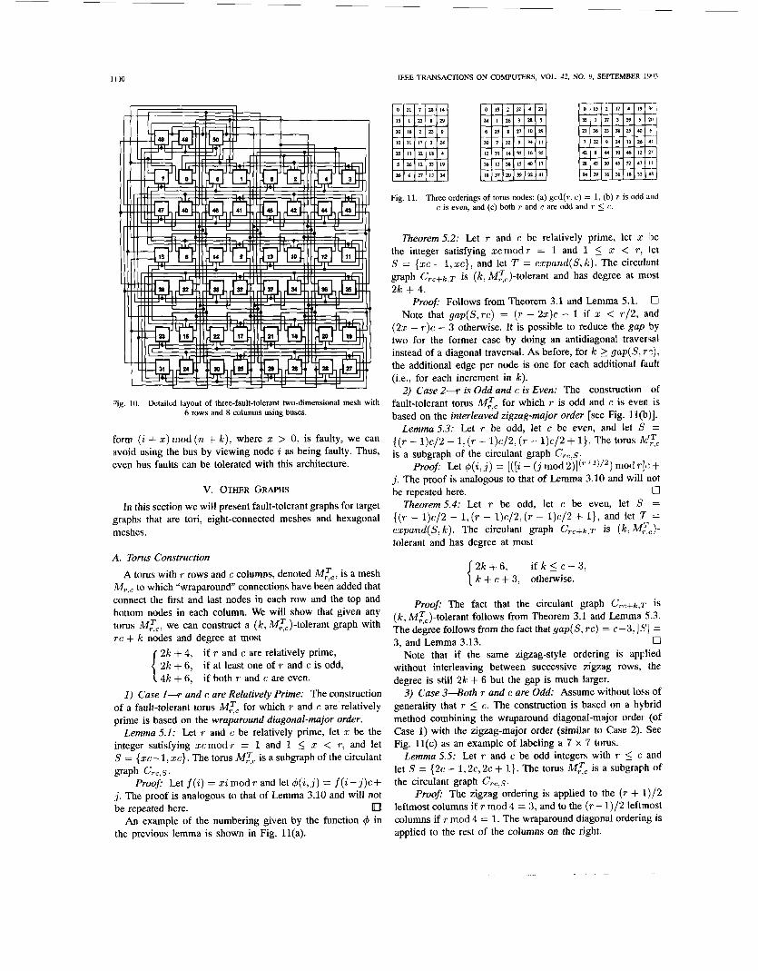
3) Implementations with Buses: Finally, we can also use buses to reduce the degree of the fault-tolerant architectures. For example, when k is odd and the target graph is a two-dimensional mesh M with r rows and c columns, the fault-tolerant graph f i k given by Corollary 4.7 is a circulant graph with offsets 1, 2 , . . . ~ ( k + 1)/2 and e, e-+ 1,. . . , c + ( k - 1)/2. However, for each healthy node i in Mk,, the target mesh M will use only at most one of the edges of the form (i, ( i + x) mod (n + k ) ) , where 1 I x I ( k + 1)/2, and at most one of the edges of the form ( i , (z + x) mod (n + k ) ) , where c 5 x 5 c + ( k - 1)/2. As a result, we can use a bus to connect each node i in &fk to all of the nodes of the form ( i+x) mod ( n + k ) , where 1 5 z 5 (k+1) /2 , and we can use a separate bus to connect node i to all of the nodes of the form ( i+x) mod ( n + k ) , where 1 5 z I c+(k-1)/2. An example of the case k = 3 is shown in Fig. 10. Note that the layout is quite compact and that most of the connections are short. Although a few of the connections appear to be relatively long in the figure, they are, in fact, of constant length and need not be made longer to create larger meshes.

A similar approach can also be used when k is even and when d > 2. In general, the use of buses results in a fault- tolerant architecture with degree at most d(k + 3)/2 if k is odd and d(k + 4)/2 if k is even. Note that if the bus connecting node i to some set of consecutive nodes of the

11 M

3

'ig. 10. Detailed layout of three-fault-tolerant two-dimensional mesh with 6 rows and 8 columns using buses.

form ( i + x) mod (n + k ) , where x > 0, is faulty, we can avoid using the bus by viewing node i as being faulty. Thus, even bus faults can be tolerated with this architecture.

V. OTHER GRAPHS In this section we will present fault-tolerant graphs for target

graphs that are tori, eight-connected meshes and hexagonal meshes.

A. Torus Construction

A torus with r rows and c columns, denoted MKc, is a mesh Mr,c to which "wraparound" connections have been added that connect the first and last nodes in each row and the top and bottom nodes in each column. We will show that given any torus MTc, we can construct a (k,MT,)-tolerant graph with r c + k nodes and degree at most

2k + 4, 2k + 6,

if r and c are relatively prime, if at least one of r and c is odd, { 4k + 6, if both r and c are even.

1) Case 1-r and c are Relatively Prime: The construction of a fault-tolerant torus MKc for which r and c are.relatively prime is based on the wraparound diagonal-major order.

Lemma 5.1: Let T and c be relatively prime, let x be the integer satisfying x c m o d r = 1 and 1 5 x < r, and let S = {zc-1, xc}. The torus MTc is a subgraph of the circulant graph crc,s.

Proof: Let f ( i ) = xamodr and let 4(i,j) = f ( z - j ) c + j. The proof is analogous to that of Lemma 3.10 and will not be repeated here.

An example of the numbering given by the function 4 in the previous lemma is shown in Fig. ll(a).

IEEE TRANSACTIONS ON COMPUTERS, VOL. 42, NO. 9, SEFEMBER 1913

Fig. 11. Three orderings of torus nodes: (a) gcd(r, c ) = 1. (b) r is odd and c is even, and (c) both T and c are odd and r 5 c.

Theorem 5.2: Let r and c be relatively prime, let x be the integer satisfying x c m o d r = 1 and 1 5 x < r, let S = {xc - l ,xc}, and let T = ezpand(S,k). The circulant graph Crc+k,T is (k, MKc)-tolerant and has degree at most 2k + 4.

Proof: Follows from Theorem 3.1 and Lemma 5.1. 0 Note that gup(S,rc) = ( r - 2x)c - 1 if x < r /2 , and

(ax - r ) c - 3 otherwise. It is possible to reduce the gap by two for the former case by doing an antidiagonal traversal instead of a diagonal traversal. As before, for k 2 gap(S, rc) , the additional edge per node is one for each additional fault @e., for each increment in k).

2) Case 2 4 is Odd and c is Even: The construction of fault-tolerant torus MTc for which r is odd and c is even is based on the interleaved zigzag-major order [see Fig. ll(b)].

Lemma5.3: Let r be odd, let c be even, and let S = { ( r - 1)c/2 - 1, ( r - is a subgraph of the circulant graph CrC,s.

Proof: Let 4 ( i , j ) = [ ( [ i - (jm0d2)]( '+~)/~)modr], :+ j . The proof is analogous to that of Lemma 3.10 and will not be repeated here. 0

Theorem 5.4: Let r be odd, let c be even, let S = { ( r - l )c /2 - 1, ( r - l )c /2 , ( r - l )c /2 + l}, and let T = expand(S, IC). The circulant graph Crc+k,T is (IC, ~4::~)- tolerant and has degree at most

( r - 1)c/2 + I}. The torus

if k 5 c - 3, { ?:c> 3, otherwise.

Proof: The fact that the circulant graph Crc+k ,~ is ( k , MTc)-tolerant follows from Theorem 3.1 and Lemma 5.3. The degree follows from the fact that gap(S, rc ) = c-3,)6'1 =

Note that if the same zigzag-style ordering is apFlied without interleaving between successive zigzag rows, the degree is still 2k + 6 but the gap is much larger.

3) Case 3 4 0 t h r and c are Odd: Assume without loss of generality that r 5 c. The construction is based on a hybrid method combining the wraparound diagonal-major ordei (of Case 1) with the zigzag-major order (similar to Case 2). See Fig. l l (c ) as an example of labeling a 7 x 7 torus.

Lemma 5.5: Let r and c be odd integers with r 5 c and let S = {2c - 1,2c, 2c + 1). The torus MTc is a subgraph of the circulant graph CrC,S.

Proof: The zigzag ordering is applied to the (T + 1)/2 leftmost columns if r mod 4 = 3, and to the ( r - 1)/2 leftmost columns if r mod 4 = 1. The wraparound diagonal ordering is applied to the rest of the columns on the right.

3, and Lemma 3.13. 0

BRUCK et ul,: FAULT-TOLERANT MESHES AND HYPERCUBES

‘(2’’) = ‘

1101

r + l 2

r - 1

i f r m o d 4 = 3 a n d j 2 -. f 2 ( i - ( j m o d 2 ) ) c + j ,

i f r m o d 4 = 1and.j < O .

Formally, let f l ( i ) = i ( r - 2) mod r, let f 2 ( i ) = 27 mod r, and let

‘(2’’) = I ~ ( z - ( j mod 2 ) ) ~ + .i.

i f r m o d 4 = 3 a n d j < 7, r + l I’ r + l i f r m o d 4 = 3 a n d j 2 -

2 .

r - 1 i f r m o d 4 = 1and.j < O .

f 2 ( i - ( j m o d 2 ) ) c + j ,

, I

- j + y ) c + j ,

It is straightforward to verify that 4 defines an embedding of

Theorem5.6: Let r and c be odd and 7‘ 5 e. let S = (2c - 1,2c, 2c + l) , and let T = erpand(S , k ) . The circulant graph C r c + k , ~ is (k,MTc)-tolerant and has degree at most 2k + 6.

Proof: The fault tolerance of C r c + k . ~ follows from Theorem 3.1 and Lemma 5.5. Since T = (2c- 1 , 2 c , . . . , 2 c + k+1) , the degree of C r c + b , ~ is Iclose(T.rc+k)l = 2 k + 6 . 0

4) Case 4 4 0 t h r and c are Even: In this case, we simply use row-major order as used in Section 111-A for the first fault- tolerant mesh construction. The proof of the following lemma is analogous to that of Lemma 3.2 and will not be included.

Lemma 5.7: Let S = (1 , c - 1 , ~ ) . The torus M:c is a subgraph of the circulant graph CrC,s.

Theorem 5.8: Let S = (1,. - 1,c) and let T = ezpand(S, k ) . The circulant graph C r c + k , ~ is ( k , MTc)- tolerant and has degree at most 4k + 6.

Proof: Follows from Theorem 3.1 and Lemma 5.7. 0 Note that Theorem 5.8 does not require that T and e have any

special properties. Finally, it should be noted that some of the constructions for fault-tolerant meshes can also be used to add fault tolerance to twisted torus networks [ 181. For example, Mesh Construction 2 presented in Theorem 3.5 yields a degree 2k + 4 fault-tolerant singly twisted torus when r = e.

MTc into Crc,s. 0

B. Eight-Connected Meshes

An eight-connected mesh with r rows and c columns, denoted M:,,,, is a mesh Mr,c to which connections between nodes that are diagonal or antidiagonal neighbors have been added. We will use row-major order to construct its fault- tolerant graph. The proofs are analogous to those of the previous section and are omitted.

Lemma 5.9: Let S = ( 1 , c - 1 , c , c + 1). The eight- connected mesh M:,,. is isomorphic to the diagonal graph

Theorem 5.10: Let S = (1.c - l . c , c + 1) and let T = ezpand(S , L k / 2 ] ) . If r > 3, the circulant graph C r c + k . ~ is ( k , M:,c) tolerant and has degree at most 2k + 6 if k is odd and 2k + 8 if k is even.

Drc,s.

Fig. 12. Wraparound hexagonal mesh of order 4

C. Hexagonal Meshes

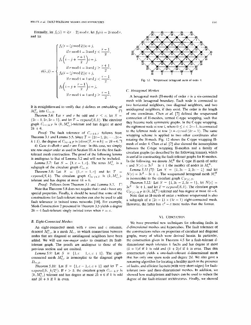
A hexagonal mesh (H-mesh) of order c is a six-connected mesh with hexagonal boundary. Each node is connected to two horizontal neighbors, two diagonal neighbors, and two antidiagonal neighbors, if they exist. The order is the length of one coordinate. Chen et al. [7] defined the wraparound connection of H-meshes, termed C-type wrapping, such that they become node symmetric graphs. In the C-type wrapping, the rightmost node at row a , where 0 5 z < 2c- 1, is connected to the leftmost node at row ( z + e ) mod (2c - 1). The same wrapping scheme is applied to two other coordinates after rotating the H-mesh. Fig. 12 shows the C-type wrapping H- mesh of order 4. Chen et al. [7] also showed the isomorphism between the C-type wrapping H-meshes and a family of circulant graphs (as described by the following lemma), which is useful in constructing the fault-tolerant graphs for H-meshes. In the following, we denote M/ the C-type H-mesh of order c and N ( c ) = 3c2 - 3c + 1 the number of nodes in M F .

Lemma 5.11 [7]: Let S = (1,3c - 2,3c - 1) and let N ( c ) = 3c2 - 3c + 1. The wraparound hexagonal mesh M P is isomorphic to the circulant graph CN(~),S.

Theorem 5.12: Let S = (1 ,3c - 2,3c - l), let N ( c ) = 3c2 - 3c + 1, and let T = erpand(S, k ) . The circulant graph C , V ( ~ ) + ~ , T is ( k , MF)-tolerant and has degree at most 4k + 6.

Note that an H-mesh of order c without wraparound is also a subgraph of a (2( - 1) x (2c - 1) eight-connected mesh. However, the latter has c2 - c more nodes than the former.

VI. CONCLUSION

We have presented new techniques for tolerating faults in d-dimensional meshes and hypercubes. The fault tolerance of the constructions relies on properties of circulant and diagonal graphs, many of which were derived herein. In particular, the construction given in Theorem 4.5 for a fault-tolerant d- dimensional mesh tolerates k faults and has degree at most ( k + 1)d if k is odd and ( k + 2)d if k is even. Thus this construction yields a one-fault-tolerant d-dimensional mesh that has only one spare node and degree 2d . We also gave a renaming algorithm for locating a healthy mesh in the presence of faults, and efficient layouts (with very short edges) for fault- tolerant two- and three-dimensional meshes. In addition, we showed how multiplexers and buses can be used to reduce the degree of the fault-tolerant architectures. Finally, we showed

, 02 IEEE TRANSACTIONS ON COMPUTERS, VOL. 42, NO. 9, SEPTEMBER l‘J93

how similar techniques can be used to obtain fault-tolerant tori, eight-connected meshes and hexagonal meshes.

APPENDIX This appendix presents the proof of Theorem 3.8. The proof

r :quires the following definitions and lemmas. Definitions: Any node ( i , j ) is a mesh Mr,c will be called

even if i+j is even, and odd otherwise. The graph Lr,c consists ( f the [rc/21 even nodes in Mr,c. Any pair of nodes ( 2 1 , jl) and (i2,jz) in Lr,c are adjacent iff Jil - 221 + Ij, - j 2 l = 2, Note that any pair of nodes adjacent in Lr,c are connected by ii path of length 2 in Mr,c. Given a set S of nodes in L,,,, t i e diagonal compression of S , denoted d i a g ( S ) , is the set ( lbtained by sliding the nodes in S upward along the diagonals i ntil all gaps have been removed. Similarly, the antidiagonal compression of S , denoted a n t i d i a g ( S ) , is the set obtained by sliding the nodes in S upward along the antidiagonals until ;11 gaps have been removed. More formal definitions of the diagonal and antidiagonal compression of S are as follows. For all i where 1 - c 5 i 5 T - 1, the ith diagonal, denoted il);, is the set D; = {(z,y) E Mr,clx - y = i}. Any node i 2 . j ) in Lr,c is in d i a g ( S ) if and only if either i 5 j and

n SI. Similarly, for all i where 0 5 i 5 T + c - 2, the ith antidiagonal, denoted Ai, Is the set Ai = {(z,y) E M,,clz + y = i}. Any node ( i , j ) i n Lr>c is in a n t i d i a g ( S ) if and only if either i + j < c and ’, < I.4;+j nSI or i + j 2 c and c - 1 - j < (A;+j nSI . Given i t graph G and a set S of nodes in G, the neighbors of S in ‘2 , denoted n e i g h b ( S , G), is the set of nodes in G that are not in S but are adjacent to a node in S.

LemmaAl: Let r be any positive integer and let S be m y set of nodes in Lr,r. Then J n e i g h b ( d i a g ( S ) , Lr,r)l 5 n e i g h b ( S , Lr,,)1 and ( n e i g h b ( a n t i d i a g ( S ) , Lr,r)l 5 ( n e i g h b

Proofi It will be shown that J n e i g h b ( d i a g ( S ) , L , , ) ( 5 neighb( S , L,,,) I. The proof that Ineighb(ant idiag( S , L,,,) I 5 Ine ighb(S , Lr,,)I is analogous and will not be given. The proof will first show that, within each diagonal, the diagonal compression operator can only decrease the number of neighbors. As a result, the overall number of neighbors can Imly decrease.

For notational simplicity, let D; = 0 for all i where either : 5 -r or i 2 r. For all i where -T - 1 5 i 5 r + 1, et Si = S fl Di and let 5’: = d i a g ( S ) fl D;. Let a be my integer where 1 - r 5 a 5 T - 1. Let T-2 = D, fl ~ e i g h b ( S , - 2 , Lr,,,), let To = D,n(ne ighb(S , , L,,,)uS,), let T1+2 = D , n n e i g h t ~ ( S , + ~ , L , , ) , and let T = T-~UTOUT+~. Similarly, let TL2 = D, n neighb(S:-,, Lr,,), let TA = D, fl :ne ighb(S; , Lr,r)USA), let Ti2 = D, fl neighb(SA+,, Lr,r) , md let T’ = T12 U TA u Ti2.

First, it will be shown that ITL21 5 IT-2). There are three :ases:

Case 1) a 5 2 - r : In this case, D,-z = 0, so Z’L2 = T-2 = 0 and ITL2( 5 IT-21.

Case 2) 3 - T 5 a 5 0 : In this case, IT-2) 2 ISa-zl + 2 and [Ti2( = lSA-21 + 2. However, (Sa-21 = lS:-21, so

< 1Di-j n SI or i > j and j <

s, Lr,r)I.

ITl21 I IT-21.

C a s e 3 ) 2 5 a < r - l : Inthiscase,if(Sa-21 2 ID,-Zl--l then T-2 = D, and TL2 C D,, so JTi2) I IT-2). Conversely, if [Sa-21 5 lDa-21 - 2 then IT-21 ISa-21 and ITL21 =

Next, we will show that IT61 I [TO(. If Sa = D, then TA = TO = D, and ITA1 5 [TO(. Conversely, if S, # D, then IT01 L (Sal + 1 and ITA1 = IS:( + 1. However, (Sal = (S,il,

It can also be shown that 5 1T+21. The proof is analogous to the proof that 5 IT-21 and will not be repeated. Therefore, ITL21 5 ]T-2l,]TA\ 5 IT)[, and 5 (T+21. Note that T = T-2 U TO U Tt.2, so IT1 2 max(lT-21,ITo(,IT+z(). In addition, note that IT’1 = max(lT121, ITol, [ T i 2 [ ) . As a result, IT’( 5 IYl. Furthermore, ID, n n e i g h b ( S , L,.,,,)I 2 IT1 - [Sal and ID, fl n e i g h b ( d i a g ( S ) , L,,,,)I = (T’( - IS:(. However, IS,( = ISil, SO ID, fl n e i g h b ( d i a g ( S ) , L,.,,)I 5 ID, fl n e i g h b ( S , Lp,r) l . Because a was chosen arbitrarily, the diagonal compression operation can only decrease the number of neighbors in each of the diagonals, and Ine ighb(d iag(S) , L,,r)l 5

Lemma A2: Let T be any integer greater than 3 and let S be any set of [r2/41 - 1 nodes in Lr,,,. Then ( n e i g h b ( S , Lr ,r) l 2 r.

Proof: Define the infinite sequence of sets So, SI, . . such that S = SO, for each i , O I i ,Si+l = anti d i a g ( d i a g ( S i ) ) . Let h be the smallest nonnegative integer such that sh = Sh+l (such as h is guaranteed to exist, as both the diagonal and antidiagonal compression operators only move nodes upward in the mesh). Note that sh = dzag(Sh) = Untzdiag(Sh) . In addition, note that for any node ( i , j ) E :;h,

it follows that all nodes of the form (i’,j’), where i’-j’ 5 i - j and i’ + j ’ I i + j , are also in sh.

Assume for the sake of contradiction that there exists. a column j in Lr,r such that all of the nodes in column j ,ire in sh. Let node (zlj) be the lowest node in column j of L,,, (thus, i = r - 1 if r + j is odd and i = r - 2 if r + j is even). Let T be the set of all nodes in Lr,, of the form (Z ’ , j ’ ) where z ’ - j ’ 5 2-j and z’+j ’ 5 z+j. Note that T C sh. However, it is straightforward (but tedious) to show that IT1 > IS), which is a contradiction.

Next, assume for the sake of contradiction that there exists a pair of adjacent columns j and j + 1 in Lr,r such that none of the nodes in columns j and j + 1 are in sh. Let a = j if j is even and let a = j + 1 if j is odd. Let T be the set of all nodes in Lr,r of the form (2, j ’ ) , where i’ - j ’ < -a or i’ + j ’ < a. Because ( 0 , a ) E sh, it follows that sh C T. However, ii is straightforward (but tedious) to show that IT( < (5’1, which is a contradiction.

Thus, there is no column in Lr,, that is completely contained in sh and there are no adjacent columns in L,,, that have no nodes in sh. As a result, every column contains at least one node in n e i g h b ( S h , L,,r) and Ineighb(Sh, Lr,,) L T . However, from Lemma A l , Ineighb(Sh, &,,)I I Ineighb(S, Lr,,)l. As a result, Ineighb(S, Lr,r)l T .

Theorem 3.8: Let T and c be integers where 4 I T 5 c and let Crc,s be a circulant graph that contains the mesh Mr,c its a subgraph. There exists an s E S such that 1s - (rc/2)1 2 ( - +

However, IS,-zl = ISi-21, so I lT-21.

so ITA1 5 ITol.

Ineighb(S, &,,)I. 0

11(3 BbUCK et al.: FAULT-TOLERANT MESHES AND HYPERCUBES

1) /2 if T is odd and C is even, and such that Is- ( r c / 2 ) ( 2 r / 2 ot ienvise.

(121 J. Hastad, F. T. Leighton, and M. Newman, “Fast computations using faulty hypercubes,” in Proc. 21st Annual ACM Symn on Theory c’f _ _ Computing, 1989, pp. 251-284.

[I31 J. P. Hayes, “A graph model for fault-tolerant computing systems,” IEEIC Trans. Comput., vol. C-25, no. 9, pp. 875-884, 1976. C. Kakkimanis, A. R. Karlin, F. T. Leighton, V. Milenkovic, P. Raghavan, S. Rao, C. Thomborson, and A. Tsantilas, “Asymptoticall!, tight bounds for computing with faulty arrays of processors,” in Proc 3Ist Annual IEEE Symp. on Foundaiions of Computer Science, pp

[15] S. Y. Kung, S. N. Jean, and C. W. Chang, “Fault-tolerant arra) processors using single-track switches,” IEEE Trans. C‘omput., vol. C-38. no. 4, pp. 501-514, 1989.

[16] S-Y. Kuo and W. K. Fuchs, “Efficient spare allocation for reconfigurable arrays,” IEEE Design and Test, pp. 24-31, 1987.

(171 F. T. Leighton and C. E. Leiserson, “Wafer scale integration of systolic arrays,” IEEE Trans. Computers, vol. C-34, no. 5 , pp. 448461, 1985.

(181 A. J. Martin, “The torus: An exercise in constructing a processing surface,” in Proc. 2nd Caltech Con5 on VLSI, 1981, pp. 527-531.

[I91 M. Paoli, W. W. Wong, and C. K. Wong, “Minimum k-Hamiltonian graphs, 11,” J. Graph Theory, vol. 10, pp. 79-95, 1986.

[20] Setting New Horizons. Aachen, Germany: Parsytec Computer GmbH, 1991.

[21] A. L. Rosenberg, “The Diogenes approach to testable fault-tolerant VLSI processor arrays,” IEEE Trans. Comput., vol. C-32, no. IO, pp. 902-910,

(221 A. L. Rosenberg, “Routing with permuters: Toward reconfigurable and fault-tolerant networks,” Tech. Rep. CS-1981-13, Dept. of Computer Science, Duke University, Durham, NC, 1981.

[23] A. L. Rosenberg, “On designing fault-tolerant VLSl processor arrays,” Advances in Computing Research, V O ~ . 2, pp. 181-204, 1984.

the in is [24] v. P. Roychowdhury, J. Bruck, and T. Kailath, “Efficient algorithms for reconfiguration in VLSI/WSI arrays,” IEEE Trans. Comput., vol. C-39, no, 4, pp. 480-489, 1990,

[2S] M. R. Samatham and D. K. Pradhan, “The de Bruijn multiprocessor network: A versatile network for parallel computation,” IEEE Trans. Comput., vol. 38, no. 4, pp. 567-581, 1989.

(261 M. Sami and R. Stefanelli, “Reconfigurable architectures for VLSI processing arrays,” Proc. IEEE, vol. 74, no. 5, 1986.

[27] Y. Ueoka, C. Minagawa, M. Oka, and A. Ishimoto, “A defect-tolerant design for full-wafer memory LSI,” IEEE J . Solid-State Circuits, vol. SC-19, no. 3, 1984.

[28] W. W. Wong and C. K. Wong, “Minimum k-Hamiltonian graphs,” J . Graph Theory, vol. 8, pp. 155-165, 1984.

First, we show that in any there exists an s E S such that Is - ( rc /2) l 2 r /2 . Assume for the sake (If contradiction that for all E S, Is - (../a)( < r / 2 , Let

i3. j ) be an embedding of Mr,c into c r c , S . Now consider an4 two nodes (i1,jl) and (i2,j2) which are adjacent in LF,r. Because there exists a path Of length in Mr,‘ between ( i l , . d and ( & ~ 2 ) , d W 4 ( i l > . d > 4 ( 2 2 , j 2 ) , T C ) i ?- - 1. Le q = [ r / 2 ] and assume without loss of generality that $ ! I ( ! ! , q ) = ( r /2 ) ( r - I) (no generality is lost because CFc,s is node-symmetric). Note that the distance in LF,F between ( q , q ) ant any other node in LF,r is at most r /2 . As a result, for any node ( i , j ) in Lr,,,O 5 q5(i,j) 5 2 ( r / 2 ) ( r - 1) = r2 - r. Thcrefore, given any two nodes (il,jl) and (iz,jz) that are adj,icent in L , r , 14(il,jl) - 4(iz,j2)1 5 r - 1.

l e t A be the set of [r2/41 - 1 nodes in Lr,r that have the smallest 4 values [formally, IA( = rr2/4] - 1 and for

B = neighb(A, L T , ~ ) . From Lemma A2, IBI 2 r , which implies that there exists a node (Z1,jl) E A and a node ( ’ 2 2 . j 2 ) E which is a c( ntradiction. Thus, in all cases, there exists an s E S such that Is - ( rc /2) l 2 r / 2 . N~~ odd and c is even. In this case, ( r c / 2 ) - r /2 and ( r c / 2 ) + r / 2 arc: not integers, so there must exist an s E s such that

0

285-296, 1990.

:Zllal) E A and ( 2 2 > j 2 ) A,4(i1>j1) < 4 ( 2 2 > j 2 ) ] ’ Let 1983.

such that I4(Zl,jl) - 4 ( i 2 , j 2 ) 1 2

1.9 - ( r c / 2 ) ( 2 ( r + 1)/2.

ACKNOWLEDGMENT

‘The authors would like to thank the anonymous referees for their helpful comments and suggestions.

REFERENCES

111 2. Annexstein, “Fault tolerance in hypercube-derivative networks,” in ,’roc. 1st Annual ACM Symposium on Parallel Algorithms and Architec- lures, 1989, pp. 179-188.

121 ‘1. Balasubramanian and P. Banejee, “A fault-tolerant massively paral- I el processing architecture,” J . Parallel Distributed Computing, vol. 4,

(31 1;. E. Batcher, “Design of a massively parallel processor,” IEEE Trans. (’omput., vol. C-29, no. 9, pp. 836-840, 1980.

14) b:. Beivide, E. Herrada, J. L. Balcizar, and J. Labarta, “Optimized mesh- connected networks for SIMD and MIMD architectures,” in Proc. 14th 6 nnual Int. Symp. Computer Architecture, 1987, pp. 163-170.

[5] I Bruck, R. Cypher, and C. T. Ho, “On the construction of fault-tolerant c‘ibe-connected cycles networks,” in Proc. I991 Int. Cont on Parallel f rocessing, vol. I, pp. 692493.

[O] .I Bruck, R. Cypher, and D. Soroker, “Running algorithms efficiently 11 1 faulty hypercubes,” in Proc. 2nd Annual ACM Symp. on Parallel A !gorithms and Architectures, 1990, pp. 37-44.

[ Y ] h‘.-S. Chen, K. G. Shin, and D. D. Kandlur, “Addressing, routing, and h oadcasting in hexagonal mesh multiprocessors,” IEEE Trans. Comput., \ol. C-39, no. 1, pp. 10-18, 1990.

181 S Dutt and J. P. Hayes, “On designing and reconfiguring k-fault-tolerant t i :e architectures,” IEEE Trans. Comput., vol. C-39, no. 4, pp. 490-503, l”90.

(91 S Dutt and J. P. Hayes, “Designing fault-tolerant systems using auto- m xphisms,” J . Parallel Distributed Computing, vol. 12, pp. 249-268, 1‘91.

[lo] S. Dutt and J. P. Hayes, “Some practical issues in the design of fault- to erant multiprocessors,” in Proc. 21st Int. Symp. on Fault-Tolerant C c,mputing, 1991, pp. 292-299.

(11.’ H Elspas and J. Turner, “Graphs with circulant adjacency matrices,” J . (’ I mbinutorial Theory, no. 9, pp. 297-307, 1970.

r’p. 363-383, 1987.

Jehoshua Bruck was born in Haifa, Ivael, on April 19, 1956 He received the BSc. and M.Sc degrees in electrical engineering from the Technion-Israel Institute of Technology, in 19x2 and 1985, respectively, and the Ph.D degree in electrical engineering from Stanford University in 1989

From 1982 to 1985 he was with the IBM Haifa Scientific Center, Israel In March 1989, he joined the IBM Research Divi5ion at the Almaden Research Center, San Jose, CA, where he currently

manages the Foundations of Massively Parallel Computing Group. He is also a Consulting Assistant Professor in the Stanford Univewty Electrical Engineering Department. Dr Bruck’s research Interests include parallel computing, fault-tolerant computing, error-correcting code\, and neural networks

Robert Cypher was born in Schenectady, NY, in 1959 He received the B S. degree in mathematical Sciences from Stanford University in 1982 dnd the M S and Ph D degrees in computer science from the University of Washington In 1987 md 1989. respective1 y

He is currently d Research Staff Member of the IBM Almaden Research Center dnd d Consulting Assistant Professor in the Stanford Univeruty Com- puter Science Department His rese,rrch interest\ include parallel algorithms, VLSI, fault tolerance,

and the design of interconnection networks

1104

Ching-Tien Ho received the B.S. degree in electrical engineering from National Taiwan University, Taiwan, in 1979 and the M.S., M.Phil., and Ph.D. degrees in computer science from Yale University, New Haven, CT, in 1985, 1986, and 1990, respectively.

Since August 1989, he has been a Research Staff Member in the Foundations of Massively Parallel Computing Group at IBM, Almaden Re- search Center. His primary research interests include communication issues for interconnection networks,

graph embeddings, fault tolerance, parallel algorithms, and architectures. Dr. Ho is a corecipient of the 1986 Outstanding Paper Award of the

International Conference on Parallel Processing. He is a member of the Association for Computing Machinery and the IEEE Computer Society.

IEEE TRANSACTIONS ON COMPUTERS, VOL. 42. NO. 9, SEPTEMBER 1993

Fault-tolerant meshes and hypercubes with minimal numbers ...

Documents