Western University Western University Scholarship@Western Scholarship@Western Electronic Thesis and Dissertation Repository 12-2-2011 12:00 AM Fault Location and Incipient Fault Detection in Distribution Cables Fault Location and Incipient Fault Detection in Distribution Cables Zhihan Xu, The University of Western Ontario Supervisor: Tarlochan Sidhu, The University of Western Ontario A thesis submitted in partial fulfillment of the requirements for the Doctor of Philosophy degree in Electrical and Computer Engineering © Zhihan Xu 2011 Follow this and additional works at: https://ir.lib.uwo.ca/etd Part of the Power and Energy Commons Recommended Citation Recommended Citation Xu, Zhihan, "Fault Location and Incipient Fault Detection in Distribution Cables" (2011). Electronic Thesis and Dissertation Repository. 319. https://ir.lib.uwo.ca/etd/319 This Dissertation/Thesis is brought to you for free and open access by Scholarship@Western. It has been accepted for inclusion in Electronic Thesis and Dissertation Repository by an authorized administrator of Scholarship@Western. For more information, please contact [email protected].

Welcome message from author
This document is posted to help you gain knowledge. Please leave a comment to let me know what you think about it! Share it to your friends and learn new things together.
Transcript
Western University Western University
Scholarship@Western Scholarship@Western
Electronic Thesis and Dissertation Repository
12-2-2011 12:00 AM
Fault Location and Incipient Fault Detection in Distribution Cables Fault Location and Incipient Fault Detection in Distribution Cables
Zhihan Xu, The University of Western Ontario
Supervisor: Tarlochan Sidhu, The University of Western Ontario
A thesis submitted in partial fulfillment of the requirements for the Doctor of Philosophy degree
in Electrical and Computer Engineering
© Zhihan Xu 2011
Follow this and additional works at: https://ir.lib.uwo.ca/etd
Part of the Power and Energy Commons
Recommended Citation Recommended Citation Xu, Zhihan, "Fault Location and Incipient Fault Detection in Distribution Cables" (2011). Electronic Thesis and Dissertation Repository. 319. https://ir.lib.uwo.ca/etd/319
This Dissertation/Thesis is brought to you for free and open access by Scholarship@Western. It has been accepted for inclusion in Electronic Thesis and Dissertation Repository by an authorized administrator of Scholarship@Western. For more information, please contact [email protected].
FAULT LOCATION AND INCIPIENT FAULT DETECTION IN DISTRIBUTION CABLES
(Spine title: Fault Location and Incipient Fault Detection in Distribution Cables)
(Thesis format: Monograph)
by
Zhihan Xu
Graduate Program in Engineering Science Department of Electrical and Computer Engineering
A thesis submitted in partial fulfillment of the requirements for the degree of
Doctor of Philosophy
The School of Graduate and Postdoctoral Studies The University of Western Ontario
London, Ontario, Canada
© Zhihan Xu, 2011
ii
THE UNIVERSITY OF WESTERN ONTARIO School of Graduate and Postdoctoral Studies
CERTIFICATE OF EXAMINATION
Supervisor ______________________________ Dr. Tarlochan Sidhu
Examiners ______________________________ Dr. Yuan Liao ______________________________ Dr. Kazimierz Adamiak ______________________________ Dr. Anestis Dounavis ______________________________ Dr. Jin Zhang
The thesis by
Zhihan Xu
entitled:
Fault Location and Incipient Fault Detection in Distribution Cables
is accepted in partial fulfillment of the requirements for the degree of
Doctor of Philosophy
______________________ _______________________________ Date Chair of the Thesis Examination Board

iii
Abstract
A set of fault location algorithms for underground medium voltage cables, two incipient fault
detection schemes for distribution cables and a state estimation method for underground
distribution networks are developed in this thesis.
Two schemes are designed to detect and classify incipient faults in underground distribution
cables. Based on the methodology of wavelet analysis, one scheme is to detect the fault-
induced transients, and therefore identify the incipient faults. Based on the analysis of the
superimposed fault current and negative sequence current in time domain, the other scheme
is particularly suitable to detect the single-line-to-ground incipient faults, which are mostly
occurring in underground cables. To verify the effectiveness and functionalities of the
proposed detection algorithms, different fault conditions, various system configurations, real
field cases and normal operating transients are examined. The simulation results have
demonstrated a technical feasibility for practical implementations of both schemes.
Based on the methodology of the direct circuit analysis, a set of location algorithms are
proposed to locate the single phase related faults in the typical underground medium voltage
cables. A large number of complex equations are effectively solved to find the fault distance
and fault resistance. The algorithms only utilize the fundamental phasors of three-phase
voltages and currents recorded at single end, normally at substation. The various system and
fault conditions are taken into account in the development of algorithms, such as effects of
shunt capacitance, mutual effects of metallic sheaths, common sheath bonding methods and
different fault scenarios. The extensive simulations have validated the accuracy and
effectiveness of the proposed algorithms.
In order to extend the proposed fault location algorithms to underground distribution
networks, a state estimation algorithm is developed to provide the necessary information for
the location algorithms. Taking account of the complexity and particularity of cable circuits,
the problem of the state estimation is formulated as a nonlinear optimization problem that is
solved by the sequential quadratic programming technique. The simulation studies have
indicated that the proposed fault location scheme incorporating with the state estimation
algorithm can achieve good performance under different load and fault conditions.

iv
Keywords
Fault Location, Distribution State Estimation, Incipient Fault Detection, Underground
Medium Voltage Cables.

v
Acknowledgments
I would like to express my deepest gratitude to my advisor Dr. Tarlochan S. Sidhu for his
advice, encouragement and guidance throughout my studies at the University of Western
Ontario. Without his support and patience, this research would have never been possible.
I am grateful to the advisory committee members, Dr. Liao, Dr. Adamiak, Dr. Dounavis and
Dr. Zhang, for their careful reading of the thesis and insightful technical suggestions.
Sincere thanks are owed to all the fine people, especially at the power group in the
Department of Electrical and Computer Engineering, who have made my time here
enjoyable.
Thanks are due to my mentor and friend, Mr. Xiaochuan Liu. Thank you for allowing me the
opportunity to learn from you, listening to me patiently, answering me accordingly and
helping me generously.
Finally, I would like to extend my heartfelt gratitude to my parents, my wife Wei and my son
Ray, for their love, support, encouragement, understanding and patience. They are the
foundation for who I am, and anything I have been able to accomplish is a tribute to them.
vi
Table of Contents
CERTIFICATE OF EXAMINATION ........................................................................... ii
Abstract .............................................................................................................................. iii
Acknowledgments............................................................................................................... v
Table of Contents............................................................................................................... vi
List of Tables ..................................................................................................................... xi
List of Figures .................................................................................................................. xiii
List of Appendices ............................................................................................................ xx
List of Symbols ................................................................................................................ xxi
Nomenclature................................................................................................................. xxiv
Chapter 1............................................................................................................................. 1
1 Introduction.................................................................................................................... 1
1.1 Incipient Fault Detection Methods.......................................................................... 1
1.2 Fault Location Methods for Cables......................................................................... 3
1.2.1 Offline Methods .......................................................................................... 3
1.2.2 Online Methods........................................................................................... 5
1.3 Fault Location Methods for Distribution Networks................................................ 9
1.3.1 Technical Cruces in Selected Location Methods...................................... 14
1.3.2 Summary of Line Model........................................................................... 18
1.3.3 Summary of Load Model .......................................................................... 21
1.3.4 Existing Limitations and Problems........................................................... 22
1.4 Distribution State Estimation Methods................................................................. 24
1.5 Objectives of the Thesis........................................................................................ 25
1.6 Contributions of the Thesis................................................................................... 26
1.7 Scope of the Thesis ............................................................................................... 27
vii
Chapter 2........................................................................................................................... 29
2 Incipient Fault Detection Schemes for Distribution Cables......................................... 29
2.1 Background........................................................................................................... 29
2.1.1 Incipient Faults in Cables.......................................................................... 29
2.1.2 Model of Arc............................................................................................. 32
2.2 Wavelet-based Detection Scheme......................................................................... 34
2.2.1 Principles................................................................................................... 34
2.2.2 System Description ................................................................................... 35
2.2.3 Detection and Classification Rules ........................................................... 40
2.2.4 Thresholds................................................................................................. 42
2.3 Superimposed Components-based Detection Scheme.......................................... 43
2.3.1 Detection of Transient Inception .............................................................. 43
2.3.2 Selection of Faulty Phase.......................................................................... 49
2.3.3 Classification............................................................................................. 53
2.3.4 Thresholds................................................................................................. 53
2.4 Simulations ........................................................................................................... 54
2.4.1 Configuration of Simulation System ........................................................ 54
2.4.2 Test Systems ............................................................................................. 55
2.4.3 Cases Studied ............................................................................................ 57
2.4.4 Simulation Results .................................................................................... 58
2.4.5 Results Using Field Recorded Data .......................................................... 62
Chapter 3........................................................................................................................... 69
3 Fault Location Algorithms for Medium Voltage Cables ............................................. 69
3.1 Background........................................................................................................... 70
3.1.1 Structure of a Typical XLPE Cable .......................................................... 70
3.1.2 Sheath Bonding Methods.......................................................................... 71
viii
3.1.3 Complexities in Fault Location for Cables ............................................... 72
3.1.4 Fault Scenarios.......................................................................................... 73
3.2 Model of Cable ..................................................................................................... 74
3.3 Location Algorithm for Cables with SPBS........................................................... 78
3.3.1 Problem Formulation ................................................................................ 78
3.3.2 Locating Core-Sheath-Ground Fault......................................................... 82
3.3.3 Locating Core-Ground Fault..................................................................... 91
3.3.4 Locating Core-Sheath Fault ...................................................................... 92
3.3.5 General Location Scheme......................................................................... 93
3.4 Location Algorithm for Cables with SPBR .......................................................... 94
3.4.1 Differences from SPBS............................................................................. 94
3.4.2 Similarities with SPBS.............................................................................. 96
3.5 Location Algorithm for Cables with SPBM ......................................................... 97
3.5.1 Fault in the First Half Section................................................................... 97
3.5.2 Fault in the Second Half Section ............................................................ 104
3.5.3 Location Scheme for Entire Cable.......................................................... 105
3.6 Location Algorithm for Cables with SBBE........................................................ 106
3.6.1 Differences from SPBS........................................................................... 106
3.6.2 Similarities with SPBS............................................................................ 108
3.7 Location Algorithm for Cables with XB ............................................................ 109
3.7.1 Fault in the First Section......................................................................... 109
3.7.2 Fault in the Middle Section..................................................................... 116
3.7.3 Fault in the Last Section ......................................................................... 119
3.7.4 Other Issues............................................................................................. 121
3.7.5 Location Scheme for Entire Cable.......................................................... 121
3.8 Summary of Location Algorithms ...................................................................... 122
ix
3.9 Load Impedance Estimation ............................................................................... 125
3.9.1 Constant Impedance Load Model ........................................................... 125
3.9.2 Static Response Load Model .................................................................. 128
3.10 Simulations ........................................................................................................ 129
3.10.1 Test Cases ............................................................................................... 129
3.10.2 Simulation Results .................................................................................. 129
3.10.3 Summary of Effects ................................................................................ 150
Chapter 4......................................................................................................................... 152
4 Extension of the Proposed Fault Location Algorithms to Medium Voltage Cables in Distribution Networks................................................................................................ 152
4.1 Background......................................................................................................... 153
4.1.1 Complexities in Fault Location in Distribution Networks...................... 153
4.1.2 Complexities in State Estimation for Distribution Networks ................. 153
4.1.3 Emerging Issues Caused by Extension to Distribution Networks .......... 154
4.1.4 Introduction to Sequential Quadratic Programming ............................... 155
4.2 Development of State Estimation Algorithm...................................................... 156
4.2.1 Problem Formulation .............................................................................. 156
4.2.2 State Estimation Algorithm..................................................................... 156
4.3 General Location Procedure Combined with State Estimation .......................... 161
4.3.1 Prefault Load Estimation by DSE........................................................... 163
4.3.2 Estimation of Quantities during Fault..................................................... 165
4.3.3 Determination of Faulty Section............................................................. 177
4.3.4 Fault Location ......................................................................................... 188
4.3.5 Summary of Location Procedure ............................................................ 188
4.4 Application of Static Response Load Model ...................................................... 189
4.5 Simulations ......................................................................................................... 190
x
4.5.1 Test System and Cases............................................................................ 190
4.5.2 Performance Indices................................................................................ 193
4.5.3 State Estimation Results ......................................................................... 194
4.5.4 Fault Location Results ............................................................................ 196
Chapter 5......................................................................................................................... 219
5 Conclusions and Future Works .................................................................................. 219
5.1 Conclusions......................................................................................................... 219
5.2 Future Works ...................................................................................................... 223
References....................................................................................................................... 225
Appendices...................................................................................................................... 234
xi
List of Tables
Table 1.1: Summary of Fault Location Methods for Distribution Networks – I .................... 10
Table 1.2: Summary of Fault Location Methods for Distribution Networks - II ................... 12
Table 2.1: Detection and Classification Results (Wavelet-based Scheme) ............................ 59
Table 2.2: Detection and Classification Results (Superimposed Components-based Scheme)
................................................................................................................................................. 62
Table 3.1: Decision of Fault Scenarios in Theory .................................................................. 74
Table 3.2: List of Unknown Variables – SPBS & CSGF ....................................................... 81
Table 3.3: List of Equations – SPBS & CSGF ....................................................................... 81
Table 3.4: List of Unknown Variables – SPBS & CGF ......................................................... 92
Table 3.5: List of Equations – SPBS & CGF ......................................................................... 92
Table 3.6: List of Unknown Variables – SPBS & CSF .......................................................... 93
Table 3.7: List of Equations – SPBS & CSF .......................................................................... 93
Table 3.8: Decision of Fault Scenarios in Practice ................................................................. 94
Table 3.9: List of Unknown Variables – SPBM-1 & CSGF................................................. 100
Table 3.10: List of Equations – SPBM-1 & CSGF............................................................... 101
Table 3.11: List of Unknown Variables – XB & CSGF....................................................... 113
Table 3.12: List of Equations – XB & CSGF ....................................................................... 113
Table 3.13: Summary of Algorithms for Single Point Bonding ........................................... 123
Table 3.14: Summary of Algorithms for Solid and Cross Bonding ..................................... 124
Table 3.15: Average of Absolute Values of Location Errors ............................................... 130
xii
Table 3.16: Distribution of Absolute Values of Location Errors.......................................... 147
Table 3.17: Effects of Bonding Methods and Fault Types on Location Accuracy............... 151
Table 4.1: Category of Sub-Algorithms................................................................................ 166
Table 4.2: Estimation of Nodal Voltages and Branch Currents............................................ 174
Table 4.3: Details of Test System......................................................................................... 191
Table 4.4: Performance Indices for Initial Loads ................................................................. 194
Table 4.5: Performance Indices for Estimated Loads........................................................... 195
Table 4.6: Percent Reduction in Error - Load Estimation .................................................... 196
Table 4.7: Average of Absolute Values of Location Errors – Individual Load Pattern ....... 197
Table 4.8: Distribution of Absolute Values of Relative Errors – Individual Load Pattern .. 198
Table 4.9: Distribution of Absolute Values of Absolute Errors – Individual Load Pattern . 199
Table 4.10: Average of Absolute Values of Location Errors – Combination of Load Patterns
............................................................................................................................................... 216
Table 4.11: Percent Reduction in Error – Combination of Load Patterns ............................ 217
Table 4.12: Distribution of Absolute Values of Relative Errors – Combination of Load
Patterns.................................................................................................................................. 217
Table 4.13: Distribution of Absolute Values of Absolute Errors – Combination of Load
Patterns.................................................................................................................................. 218
xiii
List of Figures
Figure 1.1: Lumped π line model............................................................................................ 19
Figure 2.1: Illustrations of water tree (WT) and electrical tree (ET) [76]. ............................. 30
Figure 2.2: Sub-cycle incipient fault....................................................................................... 32
Figure 2.3: Multi-cycle incipient fault. ................................................................................... 32
Figure 2.4: Detail and approximation coefficients after wavelet decomposition and
reconstruction.......................................................................................................................... 35
Figure 2.5: Flowchart of detection and classification procedures. ......................................... 36
Figure 2.6: Time sequence diagram........................................................................................ 38
Figure 2.7: Feeder current for the event of multi-cycle incipient fault................................... 39
Figure 2.8: Current for the event of capacitor switching. ....................................................... 39
Figure 2.9: Waveforms from Rule S1 – Phase-A-ground sub-cycle incipient fault............... 44
Figure 2.10: Waveforms from Rule S1 – Phase-A-ground multi-cycle incipient fault. ......... 45
Figure 2.11: Waveforms from Rule S1 – Phase-A-ground permanent fault. ......................... 45
Figure 2.12: Waveforms from Rule S1 – Phase-B-C permanent fault. .................................. 45
Figure 2.13: Waveforms from Rule S1 – Phase-A-B-ground permanent fault. ..................... 46
Figure 2.14: Waveforms from Rule S1 – Three-phase-ground permanent fault. ................... 46
Figure 2.15: Waveforms from Rule S1 – Capacitor switching............................................... 46
Figure 2.16: Waveforms from Rule S2 – Phase-A-ground sub-cycle incipient fault. ............ 47
Figure 2.17: Waveforms from Rule S2 – Phase-A-ground multi-cycle incipient fault. ......... 47
xiv
Figure 2.18: Waveforms from Rule S2 – Phase-A-ground permanent fault. ......................... 47
Figure 2.19: Waveforms from Rule S2 – Phase-B-C permanent fault. .................................. 48
Figure 2.20: Waveforms from Rule S2 – Phase-A-B-ground permanent fault. ..................... 48
Figure 2.21: Waveforms from Rule S2 – Three-phase-ground permanent fault. ................... 48
Figure 2.22: Waveforms from Rule S2 – Capacitor switching............................................... 49
Figure 2.23: Waveforms of IΔmg (Phase-A-ground multi-cycle fault, primary side, Δ/Y0). ... 50
Figure 2.24: Waveforms of IΔmg (Phase-A-ground multi-cycle fault, primary side, Y/Y0). ... 51
Figure 2.25: Amplitude of currents (3LG, primary side, Y/Y0). ............................................ 52
Figure 2.26: Amplitude of currents (SLG, primary side, Y/Y0). ............................................ 52
Figure 2.27: Configuration of simulation system. .................................................................. 55
Figure 2.28: Test system 1. ..................................................................................................... 56
Figure 2.29: Test system 2. ..................................................................................................... 57
Figure 2.30: Undetected sub-cycle fault (30 ohm). ................................................................ 59
Figure 2.31: Undetected multi-cycle fault (50 ohm). ............................................................. 60
Figure 2.32: Events with similar changing. ............................................................................ 61
Figure 2.33: Analysis process of a sub-cycle incipient fault (Wavelet-based)....................... 64
Figure 2.34: Analysis process of a sub-cycle incipient fault (Superimposed components-
based). ..................................................................................................................................... 65
Figure 2.35: Analysis process of a multi-cycle incipient fault (Wavelet-based).................... 66
Figure 2.36: Analysis process of a multi-cycle incipient fault (Superimposed components-
based). ..................................................................................................................................... 67
xv
Figure 3.1: Structure of a typical single-conductor XLPE cable and laid formations of three-
phase cables. ........................................................................................................................... 70
Figure 3.2: Sheath bonding methods. ..................................................................................... 71
Figure 3.3: Fault scenarios...................................................................................................... 74
Figure 3.4: Model of three single-conductor XLPE cables. There exist the mutual impedances
among all six conductors (Only the mutual impedances related to the core conductor of phase
A are shown in the dash-dot lines above). .............................................................................. 75
Figure 3.5: A CSGF in cable with SPBS. ............................................................................... 79
Figure 3.6: Conical surface to estimate current of the healthy sheath. ................................... 85
Figure 3.7: Three-dimensional illustration to estimate current of the faulty sheath............... 86
Figure 3.8: Contour of Figure 3.7 at zero planes. ................................................................... 87
Figure 3.9: A set of estimated currents of sheath A marked as round dots. ........................... 88
Figure 3.10: Example to show results of pinpoint criteria...................................................... 89
Figure 3.11: Location procedure for CSGF & SPBS.............................................................. 90
Figure 3.12: General location scheme - SPBS........................................................................ 94
Figure 3.13: A CSGF in cable with SPBM-1. ........................................................................ 98
Figure 3.14: Location scheme for entire cable - SPBM........................................................ 106
Figure 3.15: A CSGF in cable with XB-1............................................................................. 110
Figure 3.16: Location scheme for entire cable - XB............................................................. 122
Figure 3.17: Effect of fault type - SPBS. .............................................................................. 131
Figure 3.18: Effect of fault type - SPBR............................................................................... 132
Figure 3.19: Effect of fault type - SPBM.............................................................................. 133
xvi
Figure 3.20: Effect of fault type - SBBE. ............................................................................. 134
Figure 3.21: Effect of fault type - XB................................................................................... 135
Figure 3.22: Effect of bonding method - CSGF. .................................................................. 136
Figure 3.23: Effect of bonding method - CSF. ..................................................................... 138
Figure 3.24: Effect of bonding method - CGF...................................................................... 139
Figure 3.25: Effect of fault distance – SBBE&CSGF. ......................................................... 140
Figure 3.26: Effect of fault distance – XB&CGF. ................................................................ 141
Figure 3.27: Effect of fault distance – SPBM&CSF............................................................. 142
Figure 3.28: Effect of fault resistance – SPBS&CSGF. ....................................................... 144
Figure 3.29: Effect of fault resistance – SBBE&CGF.......................................................... 145
Figure 3.30: Effect of fault resistance – XB&CSF. .............................................................. 146
Figure 3.31: Calculation of fault resistance – SPBR. ........................................................... 148
Figure 3.32: Calculation of fault resistance – SPBM. .......................................................... 149
Figure 3.33: Calculation of fault resistance – SPBS............................................................. 150
Figure 4.1: Example to calculate injected power.................................................................. 159
Figure 4.2: A radial unbalanced underground distribution network..................................... 162
Figure 4.3: General circuit section to categorize sub-algorithms. ........................................ 165
Figure 4.4: Flowchart of SA4. .............................................................................................. 169
Figure 4.5: Node with no lateral and tapped load................................................................. 171
Figure 4.6: Node with tapped load and with no lateral......................................................... 172
xvii
Figure 4.7: Node with lateral and with no tapped load......................................................... 172
Figure 4.8: Node with lateral and tapped load...................................................................... 172
Figure 4.9: Calculation of seen impedance........................................................................... 173
Figure 4.10: Calculation processed on branch 1 (CSGF at branch 1). ................................. 178
Figure 4.11: Calculation processed on branch 2 (CSGF at branch 1). ................................. 178
Figure 4.12: Calculation processed on branch 14 (CSGF at branch 14). ............................. 179
Figure 4.13: Calculation processed on branch 13 (CSGF at branch 14). ............................. 180
Figure 4.14: Calculation processed on branch 15 (CSGF at branch 14). ............................. 180
Figure 4.15: Calculation processed on branch 18 (CSGF at branch 14). ............................. 181
Figure 4.16: Calculation processed on branch 21 (CSGF at branch 21). ............................. 182
Figure 4.17: Calculation processed on branch 19 (CSGF at branch 21). ............................. 182
Figure 4.18: Calculation processed on branch 20 (CSGF at branch 21). ............................. 183
Figure 4.19: Calculation processed on branch 1 (CGF at branch 1)..................................... 184
Figure 4.20: Calculation processed on branch 2 (CGF at branch 1)..................................... 184
Figure 4.21: Calculation processed on branch 14 (CGF at branch 14)................................. 185
Figure 4.22: Calculation processed on branch 13 (CGF at branch 14)................................. 185
Figure 4.23: Calculation processed on branch 15 (CGF at branch 14)................................. 186
Figure 4.24: Calculation processed on branch 18 (CGF at branch 14)................................. 186
Figure 4.25: Calculation processed on branch 21 (CGF at branch 21)................................. 187
Figure 4.26: Calculation processed on branch 19 (CGF at branch 21)................................. 187
xviii
Figure 4.27: Calculation processed on branch 20 (CGF at branch 21)................................. 188
Figure 4.28: Effect of cable length (CSGF @25%).............................................................. 200
Figure 4.29: Effect of cable length (CSF @50%)................................................................. 201
Figure 4.30: Effect of cable length (CGF @75%). ............................................................... 202
Figure 4.31: Effect of faulty section (CSGF @25%)............................................................ 203
Figure 4.32: Effect of faulty section (CSF @50%). ............................................................. 204
Figure 4.33: Effect of faulty section (CGF @75%).............................................................. 205
Figure 4.34: Effect of load profile (CSGF@50%, Generic profile). .................................... 206
Figure 4.35: Effect of load profile (CSGF@50%, Uniform profile). ................................... 207
Figure 4.36: Effect of load profile (CGF@50%, Generic profile)........................................ 208
Figure 4.37: Effect of load profile (CGF@50%, Uniform profile). ..................................... 209
Figure 4.38: Effect of fault distance (CSGF, LP1). .............................................................. 210
Figure 4.39: Effect of fault distance (CSF, LP1). ................................................................. 211
Figure 4.40: Effect of fault distance (CGF, LP1). ................................................................ 212
Figure 4.41: Effect of fault type (25%, LP2). ....................................................................... 213
Figure 4.42: Effect of fault type (50%, LP4). ....................................................................... 214
Figure 4.43: Effect of fault type (75%, LP6). ....................................................................... 215
Figure A.1: Fault currents. .................................................................................................... 234
Figure A.2: Wavefronts of traveling waves. ......................................................................... 235
Figure A.3: Illustration of propagation of traveling waves in spatiotemporal domain......... 236
xix
Figure A.4: Two dimension illustration of propagation of traveling wave. ......................... 236
Figure A.5: Bewley lattice diagram. ..................................................................................... 237
Figure A.6: Arc voltage. ....................................................................................................... 238
Figure A.7: Arc current......................................................................................................... 238
Figure A.8: Arc resistance. ................................................................................................... 238

xx
List of Appendices
Appendix A: Illustration of Traveling Wave ........................................................................ 234
Appendix B: Example of Kizilcay’s Arc Model................................................................... 237

xxi
List of Symbols
Unless otherwise specified, the following symbols are applied to the context.
Vx : Voltage phasor vector (6×1) at the location x, containing three-phase core voltage
phasors and three-phase sheath voltage phasors. The lowercase x could be s, r, f, m, p or t.
Vxu : Three-phase voltage phasor vector (3×1) of the conductor u at the location x. The
lowercase x could be s, r, f, m, p or t. The lowercase u could be c or n.
WVxu : Voltage phasor scalar of the conductor u of the phase W at the location x. The
lowercase x could be s, r, f, m, p or t. The lowercase u could be c or n. The capital W could be
A, B or C.
Ix : Current phasor vector (6×1) at location x, containing three-phase core current phasors
and three-phase sheath current phasors. The lowercase x could be s, r, f, m, p or t.
Ixu : Three-phase current phasor vector (3×1) of the conductor u at the location x. The
lowercase x could be s, r, f, m, p and t. The lowercase u could be c or n.
WIxu : Current phasor scalar of the conductor u of the phase W at the location x. The lowercase
x could be s, r, f, m, p or t. The lowercase u could be c or n. The capital W could be A, B or C.
Z: 6×6 series impedance matrix of cable circuit.
Zxu : 3×3 series impedance matrix between conductors x and u. The lowercase x and u could
be c or n.
EEzxx : Self-impedance scalar of the conductor x of the phase E. The lowercase x could be c or
n. The capital E could be A, B or C.

xxii
EFzxu : Series mutual impedance scalar between the conductor x of the phase E and the
conductor u of the phase F. The lowercase x and u could be c or n. The capital E and F could
be A, B or C.
Zload : 3×3 or 6×6 load impedance matrix. The dimension would be specified in the context.
Ezload : Load impedance scalar of the Phase E.
zxu : Series impedance scalar between the conductor x and u. The lowercase x and u could be
c or n. The phase is not specified.
Y: 6×6 shunt admittance matrix of cable circuit.
Yxu : 3×3 shunt admittance matrix between conductors x and u. The lowercase x and u could
be c or n.
EEyxx : Shunt admittance impedance scalar of the conductor x of the phase E. The lowercase x
could be c or n. The capital E could be A, B or C.
ycn : Shunt impedance scalar between the core conductor c and sheath n. The phase is not
specified.
yng : Shunt impedance scalar between the sheath n and ground g. The phase is not specified.
L: Length of a cable section (or subsection).
D: Fault distance from the sending terminal of the faulty section to the fault point.
core X: Core conductor of the phase X. The capital X could be A, B or C.
sheath X: Sheath conductor of the phase X. The capital X could be A, B or C.
j: 1−
c at subscript: quantities of core conductor

xxiii
n at subscript: quantities of sheath conductor
s at subscript: quantities at sending terminal
r at subscript: quantities at receiving terminal
f at subscript: quantities at fault point
m at subscript: quantities at middle point of cables with SPBM
p at subscript: quantities at the first joint of cables with XB
t at subscript: quantities at the second joint of cables with XB
A at superscript: Phase A
B at superscript: Phase B
C at superscript: Phase C
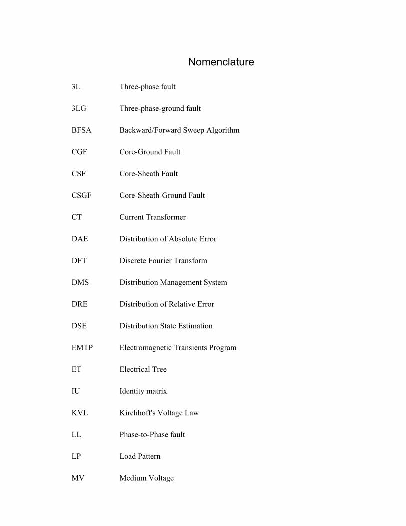
Nomenclature
3L Three-phase fault
3LG Three-phase-ground fault
BFSA Backward/Forward Sweep Algorithm
CGF Core-Ground Fault
CSF Core-Sheath Fault
CSGF Core-Sheath-Ground Fault
CT Current Transformer
DAE Distribution of Absolute Error
DFT Discrete Fourier Transform
DMS Distribution Management System
DRE Distribution of Relative Error
DSE Distribution State Estimation
EMTP Electromagnetic Transients Program
ET Electrical Tree
IU Identity matrix
KVL Kirchhoff's Voltage Law
LL Phase-to-Phase fault
LP Load Pattern
MV Medium Voltage

xxv
PE Polyethylene
PRE Percent Reduction in Error
QP Quadratic Programming
SA Sub-Algorithm
SBBE Solid Bonding at Both Ends
SE State Estimation
SLG Single-Line-Ground fault
SNR Signal Noise Ratio
SPBM Single Point Bonding at Middle Point
SPBM-1 First Half Section with Single Point Bonding at Middle Point
SPBM-2 Second Half Section with Single Point Bonding at Middle Point
SPBR Single Point Bonding at Receiving Terminal
SPBS Single Point Bonding at Sending Terminal
SQP Sequential Quadratic Programming
TDR Time Domain Reflectrometer
WLS Weighted Least Squares
WT Water Tree
XB Cross Bonding
XB-1 First Section with Cross Bonding
XB-2 Middle Section with Cross Bonding

xxvi
XB-3 Last Section with Cross Bonding
XLPE Cross-Linked Polyethylene
1
Chapter 1
1 Introduction
Underground cables have been widely applied in power distribution networks due to the
benefits of underground connection, involving more secure than overhead lines in bad
weather, less liable to damage by storms or lightning, no susceptible to trees, less
expensive for shorter distance, environment-friendly and low maintenance. However, the
disadvantages of underground cables should also be mentioned, including 8 to 15 times
more expensive than equivalent overhead lines, less power transfer capability, more
liable to permanent damage following a flash-over, and difficult to locate fault.
Faults in underground cables can be normally classified as two categories: incipient faults
and permanent faults. Usually, incipient faults in power cables are gradually resulted
from the aging process, where the localized deterioration in insulations exists. Electrical
overstress in conjunction with mechanical deficiency, unfavorable environmental
condition and chemical pollution, can cause the irreparable and irreversible damages in
insulations. Eventually, incipient faults would fail into permanent faults sooner or later.
The detection of incipient faults can provide an early warning for the breakdown of the
defective cable, even trip the suspected feeder to limit the repetitive voltage transients.
The location of permanent faults in cables is essential for electric power distribution
networks to improve network reliability, ensure customer power quality, speed up
restoration process, minimize outage time, reduce repairing cost, dispatch crews more
efficiently and maintain network reliability. The state estimation (SE) is an auxiliary tool
to provide the necessary information for the proposed location algorithms. The related
methods published in journals and proceedings are reviewed, summarized and compared
in the next subsections.
1.1 Incipient Fault Detection Methods
Comparing with the detection methods for arcing faults in overhead lines, there are
relatively fewer literatures and reports discussing the detection of incipient faults in

2
underground cables. The existing detection methods are generally based on the analysis
of waveforms rather than phasors. Basically, the process of detection is to examine the
characteristics of voltages and currents in time domain, frequency domain and time-
frequency domain.
The advantages and disadvantages of four existing techniques developed for field
applications were reviewed and evaluated from the point of a power engineer in [1].
These techniques include detection of partial discharges, time and frequency domain
reflectometry, measurements of dielectric ohmic and polarization, and acoustic and
pressure wave techniques.
Charytoniuk et al. studied the feasibility of detecting arcing faults in underground cables
[2]. An experiment was carried out in one secondary distribution network by personnel
from the Consolidated Edison Company of New York. Through analyzing the collected
data, three feasible methods are considered, i.e. analysis of voltages and currents in time
domain, in frequency domain and in time-frequency domain with the aid of the wavelet
analysis. Furthermore, it is pointed out that the potential approaches can process the
instantaneous values of currents, and combine the arc fault features in time, frequency
and time-frequency domains.
Kojovic et al. proposed an incipient cable splice failure detection scheme, which is
integrated into a universal relay platform as an additional function to enhance the
distribution feeder protection [3], [4]. The basic principle is to monitor instantaneous
overcurrent, counter the number of fault occurrences, record the frequency of fault
occurrences, and provide alarming or tripping capability.
Kasztenny et al. proposed a simple, fast and robust method for detecting incipient faults
in cables and implemented it in a commercial relay [5]. The method employs the
superimposed current components and neutral current to monitor the consistency of
currents before and after the event, find the phase where the event occurs, check the event
duration, and set the alarming or tripping signal.
3
Both the magnitude of neutral current and the magnitude of rate of change of neutral
current were used to detect self-clearing cable transient faults and distinguish them from
normal system switching as well as other system faults, such as fast fuse operations [6].
The faulty phase is selected by a phase current rate of change based detector.
The wavelet analysis and neural network were combined to detect on-line incipient
transients in underground distribution cable laterals and predict the remaining life of the
cable lateral [7]. The wavelet packet analysis technique is applied to decompose the
current into separate frequency bands and to extract features. Then, a type of artificial
neural network, self-organizing map, is used for pattern identification. Therefore, the data
sets are clustered and incipient behavior is identified and categorized.
The pattern analysis techniques were applied to classify load change transients and
incipient abnormalities in an underground distribution cable lateral [8]. A set of features
are exacted by the wavelet packet analysis and output to k-nearest-neighbor classifiers.
The methods of dimensionality reduction are used to reduce the dimensionality for the
pattern recognition and preserve the good classification accuracy as well.
1.2 Fault Location Methods for Cables
Basically, the location methods for cables are divided into the offline and online methods.
The offline methods employ the special instruments to test the out of service cable in
field. On the other hand, the online methods utilize and process the sampled voltages and
currents to determine the fault point.
1.2.1 Offline Methods
There are two offline location approaches, i.e. terminal approaches and tracer approaches.
Terminal methods rely on measurements made from either one or both terminals of the
cable to prelocate fault points approximately, but not accurately enough to allow dig.
Tracer methods rely on measurements taken along the cable to pinpoint the fault location
very accurately. Both methods are on-site technique and performed with low efficiency.
Eighteen terminal methods are introduced in [9] and listed below.
4
• Halfway Approach Method • Voltage Drop Ratio Method
• Charging Current Method • Insulation Resistance Ratio Method
• Murray Loop Method • Capacitance Ratio Method
• Murray Loop Two-End Method • Murray-Fisher Loop Method
• Varley Loop Method • Hilborn Loop Method
• Open-and-closed Loop Method • Werren Overlap Method
• Impulse Current Method • Pulse Decay Method
• Standing Wave Differential • DC Charging Current Method
• Time Domain Reflectrometer (TDR)/Cable Radar Method
• TDR/Cable Radar and Thumper Method
Following the prelocation by the terminal methods, a tracer method is generally applied
to pinpoint the fault point and this method usually requests the repair crews to walk along
the cable route. Nine tracer methods introduced in [9] are listed below.
• Magnetic Pickup Method • Tracing current Method
• Earth gradient Method • Hill-of-Potential Method
• Thumper/Acoustic Method • Thumper/Electromagnetic Wave Method
• Sheath Coil Method • Pick Method
• DC Sheath Potential Difference Method
Some extension works were proposed as an aid for the offline methods. An expert system
was developed for the Electric Power Research Institute (EPRI) [10]. The system creates
a reference manual [9] to provide the guidance for field crews to diagnose a cable failure,
recommend applicable fault location techniques, and trouble-shoot resulting difficulties
which occur during the process of locating underground cable faults.
For the sake of clarifying the results obtained from the terminal methods, an expert
system approach was proposed to locate fault on high voltage underground cable systems
[11]. The experience and expertise of many different engineers is accumulated to build a
truly expert system. With the data acquired from diagnostic tests, the system can infer the
fault type, advise the further location techniques, and conclude the probable fault location.
The operator is then advised to carry out the tracer methods to locate the fault precisely.
5
1.2.2 Online Methods
The online location methods for underground cables are comparatively fewer than the
ones applied for overhead lines. Two principal techniques have been proposed for the
online location, i.e. signal analysis and knowledge-based [12]. The former one is further
classified into the approaches based on fundamental frequency phasor quantities and high
frequency traveling waves.
1.2.2.1 Fundamental Phasor-based Methods
The fundamental phasor-based methods utilize the voltage and current phasors at the
fundamental frequency. Basically, the impedance is calculated and used to decide the
fault distance, so it is also called the impedance-based methods [13], [14].
Filomena et al. extended the traditional impedance-based location algorithms to calculate
the apparent impedance of cables in cases of single phase to ground fault (SLG) and
three-phase fault (3L) [15]. The single-end voltages and currents are used. An iterative
algorithm is proposed to compensate the capacitive characteristic in typical underground
cables. The fault location scheme can be applied in balanced or unbalanced distribution
systems with laterals and tapped loads.
Based on the estimation of the fault-loop impedance, Saha et al. presented four location
algorithms to consider the following scenarios [16]: SLG fault with measurements
available in the faulty feeder (voltages and currents), SLG fault with measurements
available at the substation level (total currents are measured at the supplying transformer),
phase to phase (LL) or 3L fault with measurements available in the faulty feeder, LL or
3L fault with measurements available at the substation. Only positive sequence
impedance calculation is needed for LL or 3L fault, while the zero-sequence impedance
calculation is required for SLG fault. The algorithms can be applied in radial medium
voltage (MV) systems, which include many intermediate load taps. The non-homogeneity
of the feeder sections is also taken into account.
The apparent seen impedance was calculated using local measuring quantities available at
substation [17]. Upon the different fault type, the different apparent impedance
6
parameters, voltage and current quantities are utilized. Then, a fault distance is estimated
using the conventional apparent impedance computation. Finally, an iterative
compensation mechanism is executed to eliminate the estimation errors caused by the
charging currents in cables. The basic procedure is similar to the work in [15] except that
the symmetrical components are used.
The location algorithm in [18] extended the traditional Takagi’s method [19] into
distribution cable networks. The sequence phase impedance model is used to model
laterals and circuit sections. The line shunt capacitance is taken into account to optimize
the result so that the major source of error in conventional impedance based methods,
particularly for cable networks, is minimized.
Differentiating from the above extended impedance-based methods, an iterative
algorithm was proposed for locating faults in cables [20]. The circuit is modeled by the
distributed parameter approach and the voltage and current equations are formulated
based on the sequence networks. The Newton–Raphson method is applied to calculate the
fault distance. The algorithm is also extended to the radial multi-section cables with
tapped loads.
A double-end based location algorithm was presented, particularly for aged power cables
[21]. The aging process in cables would cause the change of the relative permittivity and
in turn result in the changes in the positive, negative, and zero sequence capacitance. The
fault location scheme is based on phasor measurements from both ends of the cable,
incorporating with the distributed line model, Clarke transformation theory and discrete
Fourier transform (DFT).
One algorithm implemented in the Con Edison of New York was presented in [22]. The
voltages and currents are recorded by the power quality monitors and processed for
calculations in the control center. The reactance to fault is calculated based on the fault
measurements and prior knowledge of known fault information. The calculation results
combined with up-to-date distribution feeder models and geographic information system
data are used to generate the estimated fault location tables and viewing maps. The
estimation would typically take ten minutes after the inception of a fault. The location
7
accuracy is within 10% of the total number of feeder structures, for about 80% of the
single phase faults.
One more implementation in the Dutch grid operator Alliander was presented in [23],
[24]. The fault locators only use the calculated reactance since the reactance of fault
impedance is zero and the cable reactance is well known and not current dependent. Then,
the scenarios of short circuits on all nodes in the faulted feeder are simulated on an actual
network model. The calculated impedance is compared with the simulated impedances to
find the exact location. The location algorithm is known to find the distance within 5
minutes after the occurrence of a fault. The system is able to locate LL and 3L faults
within 100 meters and SLG faults within 500 meters.
1.2.2.2 Traveling wave-based Methods
Traveling waves are generated by the change of stored energy in capacitance and
inductance in lines or cables after the occurrence of a fault. Both voltage and current
traveling waves propagate along the circuit at the speed as high as the light speed until
meeting any impedance discontinuities, and then the fault-induced high frequency waves
would reflect back to the origin and transmit through towards other side.
Almost all traveling waves-based methods are based on the principle of the Bewley
lattice diagram [25], and the fault distance is calculated by the multiplication of the
propagation velocity and the interval, which is the time difference between the arrival
instant of the initial wavefront and the arrival instant of the reflected wavefront. The
basic location principle and common locator types are introduced in [26].
Appendix A visually illustrates and explains an example of the traveling wave, which is
generated by an SLG fault in a transmission line and can be used for the purpose of the
line protection and fault location.
Bo et al. designed a special transient capturing unit to extract the fault-generated high
frequency voltage transient signals in cables [27]. The principle of the fault location
method is to identify the successive arrivals of the traveling high frequency voltage
signals arriving at the busbar where the locator is installed. Particularly the first and the

8
subsequent arriving wavefronts with reference to the first wavefront are used to locate the
fault position. The above work is enhanced by applying new technique, wavelet
transform, to effectively extract a band of high frequency transient voltage signals [28].
A cable fault location scheme was proposed based on the principle of the traditional
traveling wave principle, synchronized sampling technique and wavelet analysis [29].
The current signals at the two terminals are synchronized with the help of GPS and the
arrival time of fault-induced traveling waves is precisely detected by the wavelet analysis.
Then, the location is obtained from the multiplication of the propagation velocity and the
time interval.
Similarly, based on the principle of the traditional Bewley lattice, a double-end traveling
wave fault location scheme was proposed for locating faults in aged cables [30]. The
wavelet analysis is applied to analyze the synchronized voltage singles at the two
terminals to capture the singularity in high frequency transients. The calculations are
processed with the modal quantities rather than the phase quantities. The effect of
changes in the propagation velocity of traveling wave is eliminated.
The fault section and location was determined by the analysis of traveling waves in
current signals [31]. First, the fault section is identified by the comparison between the
distance of each peak in the high frequency current signals and the known reflection
points in distribution feeders. Then, the simulation is processed with the possible location
in a transient power system simulator, which is modeled from the actual network. The
simulated currents are cross correlated with the measured currents to find the match
degree in high frequency transients of both current signals. The cross-correlation
coefficients would be a high positive value if the estimated fault location is correct.
1.2.2.3 Knowledge-based Methods
Knowledge-based techniques, such neural network, fuzzy logic and expert system, are
applied to fault location for cables. The usage of artificial intelligence techniques usually
requires the specific learning process for each analyzed feeder. Additionally, the signal
9
processing techniques can also be used to preprocess the signals and extract the features
fed into the analysis of artificial intelligence.
Sadeh et al. proposed a fault location algorithm for combined overhead transmission line
with underground power cable [32]. First, one adaptive network-based fuzzy inference
system (ANFIS) is used to classify the fault type. Then, another ANFIS is applied to
detect the faulty section, whether the fault is on the overhead line or on the underground
cable. Other eight ANFIS networks are utilized to pinpoint the fault, in which two
networks are used for one fault type. The neuro-fuzzy inference systems are trained by
the data obtained from simulations.
Moshtagh and Aggarwal proposed a location algorithm combined the neural network and
wavelet analysis [33]. The power distribution system transient signals are generated by
the EMTP software, analyzed using the wavelet analysis to extract the useful fault
features, and applied to the artificial neural networks (ANNs) for locating ungrounded
shunt faults. A three-layer feed-forward ANN with Levenberg-Marquardt learning
algorithm is used for the fault classification and fault location. One network is designed
to classify the fault type and several ANNs related to each fault type are designed to
locate the actual ungrounded fault position.
1.3 Fault Location Methods for Distribution Networks
The fault location techniques have been well developed and applied in transmission
systems. However, relatively less research work has been conducted in the development
of fault location approaches for distribution networks. An effective and accurate fault
location algorithm is essential for electric power distribution networks to locate the fault
point, improve the service reliability, ensure the customer power quality, and speed up
the restoration process. Particularly, it appears more important for locating faults in
underground distribution cables due to the complexities in electrical characteristics of
cables, underground placement environment and wide applications in high density
commercial districts.
10
Similarly, two principal techniques have been proposed for such methods, i.e., signal
analysis and knowledge-based [12]. The former one is further classified into the
approaches based on fundamental frequency phasor quantities and high frequency
traveling waves. The knowledge-based and traveling wave-based techniques have been
briefly discussed in Section 1.2.2.
The utility companies and researchers have been turning more and more attention to the
location methods only using voltages and currents recorded at substation [34]. The
fundamental phasor-based methods utilize and process the recorded voltages and currents
to determine the fault point. Since the proposed algorithm is to use the fundamental
phasors, the existing fundamental phasor-based methods would be discussed in this
subsection.
The basic location methods, such as the reactance method and Takagi method, have been
reviewed in [13], [14] and [35]. Ten most cited impedance-based fault location methods
are compared, analyzed and tested, and thereafter the main problems existing in these
methods are concluded [36]. The practical experience and the fault location systems used
in utilities are introduced in [37] and [38]. Most of the previously proposed location
techniques concern the location problem in overhead distribution lines, and a few of
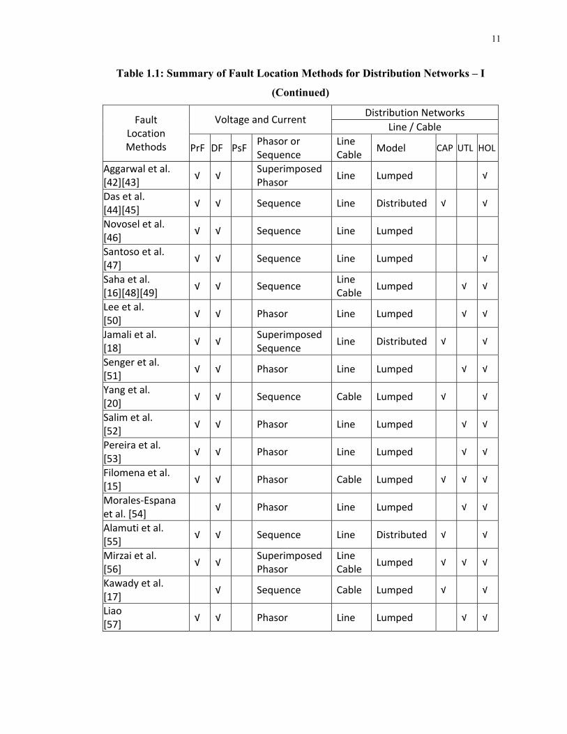
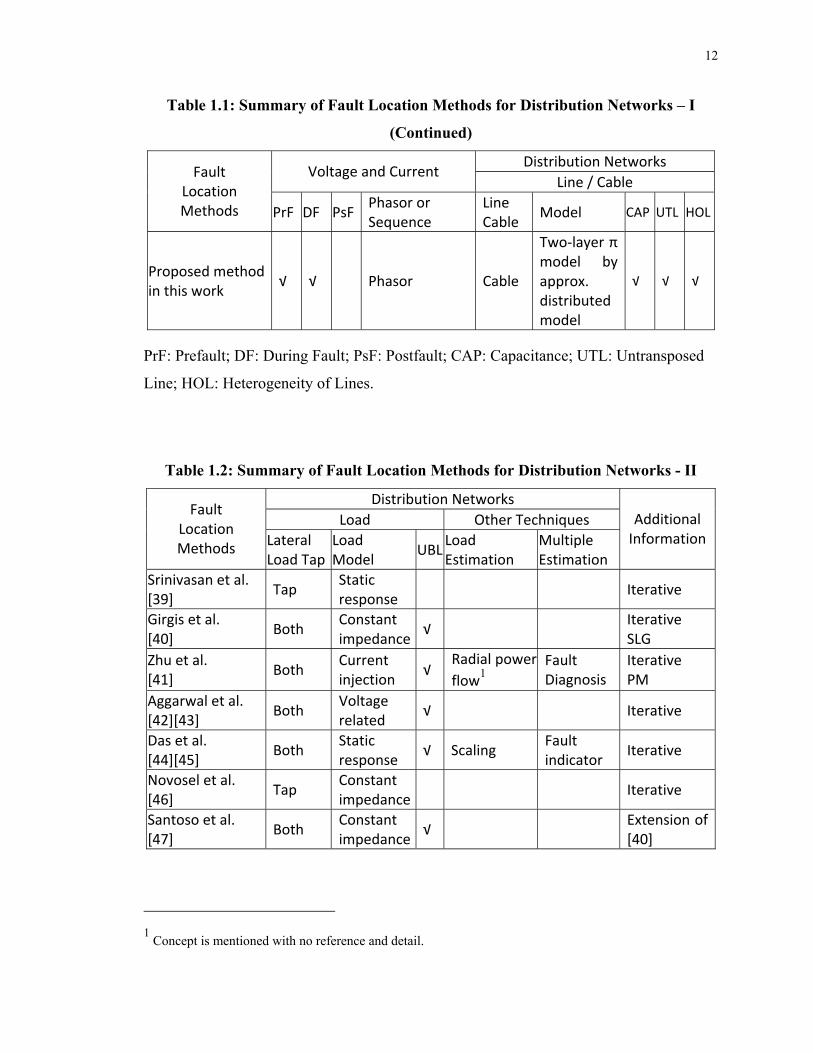
literatures discuss the algorithms for underground distribution cables. Twenty algorithms
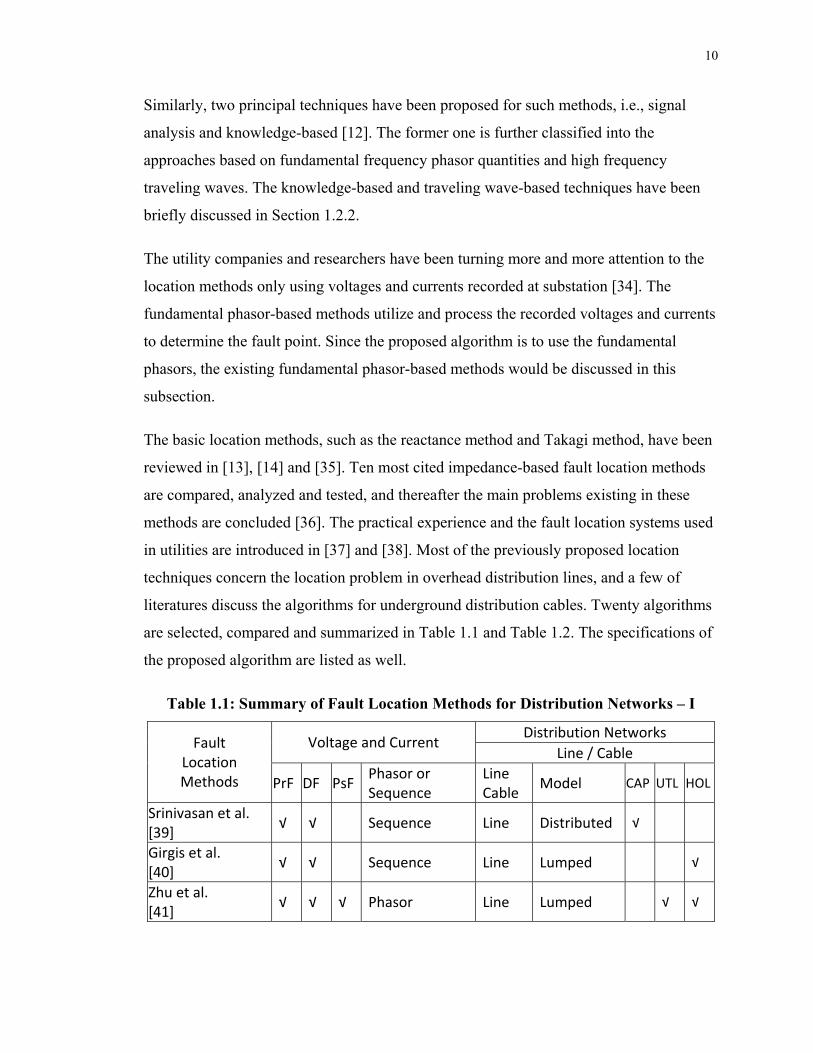
are selected, compared and summarized in Table 1.1 and Table 1.2. The specifications of
the proposed algorithm are listed as well.
Table 1.1: Summary of Fault Location Methods for Distribution Networks – I
Distribution Networks Voltage and Current Line / Cable
Fault Location Methods PrF DF PsF Phasor or
Sequence Line Cable Model CAP UTL HOL
Srinivasan et al. [39] √ √ Sequence Line Distributed √
Girgis et al. [40] √ √ Sequence Line Lumped √
Zhu et al. [41] √ √ √ Phasor Line Lumped √ √
11
Table 1.1: Summary of Fault Location Methods for Distribution Networks – I
(Continued)
Distribution Networks Voltage and Current Line / Cable
Fault Location Methods PrF DF PsF Phasor or
Sequence Line Cable Model CAP UTL HOL
Aggarwal et al. [42][43] √ √ Superimposed
Phasor Line Lumped √
Das et al. [44][45] √ √ Sequence Line Distributed √ √
Novosel et al. [46] √ √ Sequence Line Lumped
Santoso et al. [47] √ √ Sequence Line Lumped √
Saha et al. [16][48][49] √ √ Sequence Line
Cable Lumped √ √
Lee et al. [50] √ √ Phasor Line Lumped √ √
Jamali et al. [18] √ √ Superimposed
Sequence Line Distributed √ √
Senger et al. [51] √ √ Phasor Line Lumped √ √
Yang et al. [20] √ √ Sequence Cable Lumped √ √
Salim et al. [52] √ √ Phasor Line Lumped √ √
Pereira et al. [53] √ √ Phasor Line Lumped √ √
Filomena et al. [15] √ √ Phasor Cable Lumped √ √ √
Morales-Espana et al. [54] √ Phasor Line Lumped √ √
Alamuti et al. [55] √ √ Sequence Line Distributed √ √
Mirzai et al. [56] √ √ Superimposed
Phasor Line Cable Lumped √ √ √
Kawady et al. [17] √ Sequence Cable Lumped √ √
Liao [57] √ √ Phasor Line Lumped √ √
12
Table 1.1: Summary of Fault Location Methods for Distribution Networks – I
(Continued)
Distribution Networks Voltage and Current Line / Cable
Fault Location Methods PrF DF PsF Phasor or
Sequence Line Cable Model CAP UTL HOL
Proposed method in this work √ √ Phasor Cable
Two-layer π model by approx. distributed model
√ √ √
PrF: Prefault; DF: During Fault; PsF: Postfault; CAP: Capacitance; UTL: Untransposed
Line; HOL: Heterogeneity of Lines.
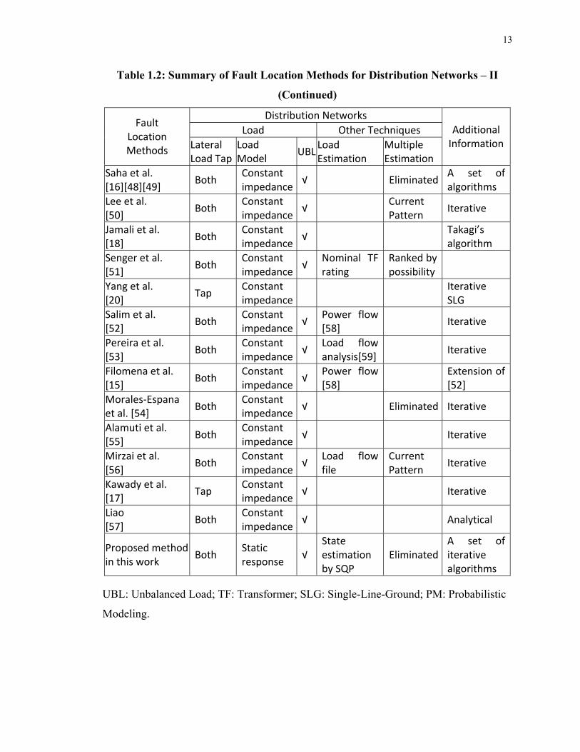
Table 1.2: Summary of Fault Location Methods for Distribution Networks - II
Distribution Networks Load Other Techniques
Fault Location Methods Lateral
Load Tap Load Model UBL Load
Estimation Multiple Estimation
Additional Information
Srinivasan et al. [39] Tap Static
response Iterative
Girgis et al. [40] Both Constant
impedance √ Iterative SLG
Zhu et al. [41] Both Current
injection √ Radial power flow1
Fault Diagnosis
Iterative PM
Aggarwal et al. [42][43] Both Voltage
related √ Iterative
Das et al. [44][45] Both Static
response √ Scaling Fault indicator Iterative
Novosel et al. [46] Tap Constant
impedance Iterative
Santoso et al. [47] Both Constant
impedance √ Extension of [40]
1 Concept is mentioned with no reference and detail.
13
Table 1.2: Summary of Fault Location Methods for Distribution Networks – II
(Continued)
Distribution Networks Load Other Techniques
Fault Location Methods Lateral
Load Tap Load Model UBL Load
Estimation Multiple Estimation
Additional Information
Saha et al. [16][48][49] Both Constant
impedance √ Eliminated A set of algorithms
Lee et al. [50] Both Constant
impedance √ Current Pattern Iterative
Jamali et al. [18] Both Constant
impedance √ Takagi’s algorithm
Senger et al. [51] Both Constant
impedance √ Nominal TF rating
Ranked by possibility
Yang et al. [20] Tap Constant
impedance Iterative SLG
Salim et al. [52] Both Constant
impedance √ Power flow [58] Iterative
Pereira et al. [53] Both Constant
impedance √ Load flow analysis[59] Iterative
Filomena et al. [15] Both Constant
impedance √ Power flow [58] Extension of
[52] Morales-Espana et al. [54] Both Constant
impedance √ Eliminated Iterative
Alamuti et al. [55] Both Constant
impedance √ Iterative
Mirzai et al. [56] Both Constant
impedance √ Load flow file
Current Pattern Iterative
Kawady et al. [17] Tap Constant
impedance √ Iterative
Liao [57] Both Constant
impedance √ Analytical
Proposed method in this work Both Static
response √ State estimation by SQP
Eliminated A set of iterative algorithms
UBL: Unbalanced Load; TF: Transformer; SLG: Single-Line-Ground; PM: Probabilistic
Modeling.
14
The voltages and/or currents measured at substation are used in all selected methods.
Most of them utilize the prefault and during-fault quantities.
The phasors, symmetrical components, and/or superimposed components of voltages and
currents are employed. However, the usage of symmetrical components restricts its
application to ideally balanced and transposed feeders, which is not true in a typical
distribution network.
The location methods for cables should take the capacitance into account since the
capacitance has significant effect on the voltage and current along cables and cannot be
ignored.
The untransposed lines and cables are very normal in a distribution system, which makes
the system unbalanced and restricts the application of symmetrical components.
Heterogeneity of feeders is characterized by the presence of multiple sections of different
size and length of overhead lines and underground cables.
The distribution network is unbalance due to the presence of single-phase, double-phase
and three-phase loads.
The laterals and tapped loads along the main feeder are presented in a typical distribution
network.
The representative technical cruces, load models and line models in selected methods are
concluded in the following subsections.
1.3.1 Technical Cruces in Selected Location Methods
The general logic principle in most of the selected algorithms, including the proposed
one, is first to determine the fault point in a single plain line or cable with no laterals and
tapped loads. Subsequently, the location algorithm is extended to distribution networks
taking account of the presence of laterals, tapped loads, unbalanced loads, and
heterogeneity of lines, etc.
15
Some very general fundamentals in the selected methods are somehow similar and
behave like a technical crux in the development of the location algorithms. However, the
principle and procedure of a specific method may appear considerable diversity, which
depends on many factors, such as locating strategy and logic, assumptions, unknown
variables, utilized quantities, applied line and load models, and particular application
environment. Three mostly used cruces in the selected location methods are explained
below. It should be mentioned that only the very basic fundamentals are introduced and
the application details may have considerable diversity and can be referred to the related
literatures.
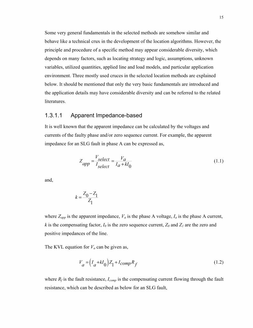
1.3.1.1 Apparent Impedance-based
It is well known that the apparent impedance can be calculated by the voltages and
currents of the faulty phase and/or zero sequence current. For example, the apparent
impedance for an SLG fault in phase A can be expressed as,
0
V Vselect aZapp I I kIaselect= = + (1.1)
and,
0 1
1
Z Zk
Z
−=
where Zapp is the apparent impedance, Va is the phase A voltage, Ia is the phase A current,
k is the compensating factor, I0 is the zero sequence current, Z0 and Z1 are the zero and
positive impedances of the line.
The KVL equation for Va can be given as,
( ) 10V I kI Z I Rcomp fa a= + + (1.2)
where Rf is the fault resistance, Icomp is the compensating current flowing through the fault
resistance, which can be described as below for an SLG fault,
16
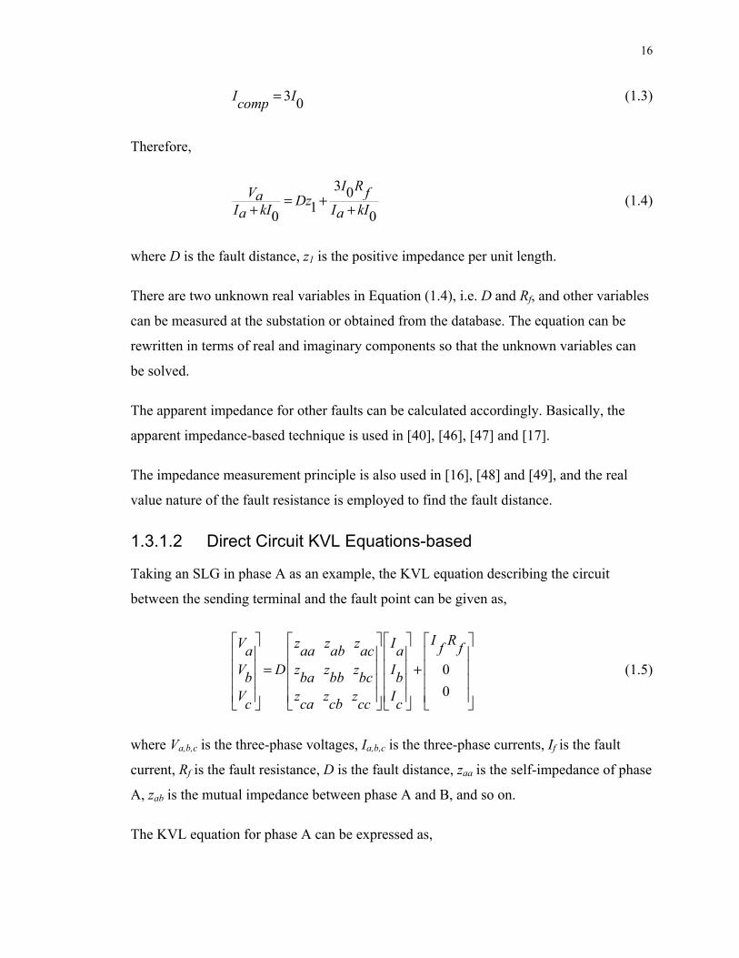
3 0I Icomp = (1.3)
Therefore,
3 01
0 0
I RV fa DzI kI I kIa a
= ++ + (1.4)
where D is the fault distance, z1 is the positive impedance per unit length.
There are two unknown real variables in Equation (1.4), i.e. D and Rf, and other variables
can be measured at the substation or obtained from the database. The equation can be
rewritten in terms of real and imaginary components so that the unknown variables can
be solved.
The apparent impedance for other faults can be calculated accordingly. Basically, the
apparent impedance-based technique is used in [40], [46], [47] and [17].
The impedance measurement principle is also used in [16], [48] and [49], and the real
value nature of the fault resistance is employed to find the fault distance.
1.3.1.2 Direct Circuit KVL Equations-based
Taking an SLG in phase A as an example, the KVL equation describing the circuit
between the sending terminal and the fault point can be given as,
0
0
I RV z z z I f fa aa ab ac aV D z z z Ib ba bb bc bV z z z Ic ca cb cc c
= +
(1.5)
where Va,b,c is the three-phase voltages, Ia,b,c is the three-phase currents, If is the fault
current, Rf is the fault resistance, D is the fault distance, zaa is the self-impedance of phase
A, zab is the mutual impedance between phase A and B, and so on.
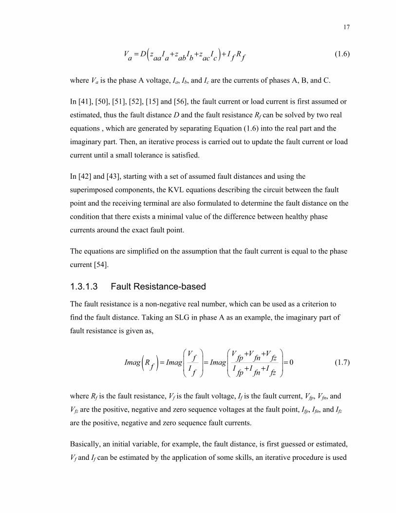
The KVL equation for phase A can be expressed as,
17
( )V D z I z I z I I Rf fa aa a ab b ac c= + + + (1.6)
where Va is the phase A voltage, Ia, Ib, and Ic are the currents of phases A, B, and C.
In [41], [50], [51], [52], [15] and [56], the fault current or load current is first assumed or
estimated, thus the fault distance D and the fault resistance Rf can be solved by two real
equations , which are generated by separating Equation (1.6) into the real part and the
imaginary part. Then, an iterative process is carried out to update the fault current or load
current until a small tolerance is satisfied.
In [42] and [43], starting with a set of assumed fault distances and using the
superimposed components, the KVL equations describing the circuit between the fault
point and the receiving terminal are also formulated to determine the fault distance on the
condition that there exists a minimal value of the difference between healthy phase
currents around the exact fault point.
The equations are simplified on the assumption that the fault current is equal to the phase
current [54].
1.3.1.3 Fault Resistance-based
The fault resistance is a non-negative real number, which can be used as a criterion to
find the fault distance. Taking an SLG in phase A as an example, the imaginary part of
fault resistance is given as,
( ) 0V V V Vf fp fn fz
Imag R Imag Imagf I I I If fp fn fz
+ + = = = + +
(1.7)
where Rf is the fault resistance, Vf is the fault voltage, If is the fault current, Vfp, Vfn, and
Vfz are the positive, negative and zero sequence voltages at the fault point, Ifp, Ifn, and Ifz
are the positive, negative and zero sequence fault currents.
Basically, an initial variable, for example, the fault distance, is first guessed or estimated,
Vf and If can be estimated by the application of some skills, an iterative procedure is used
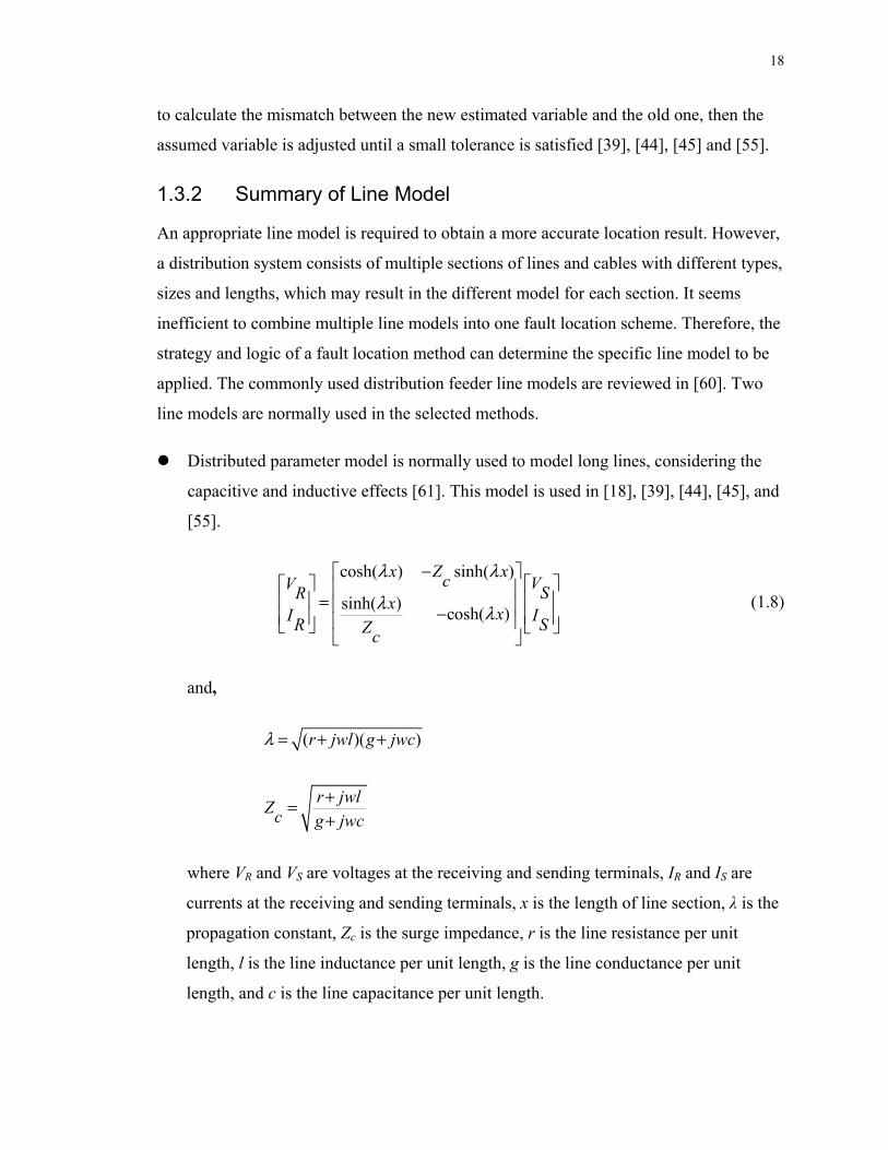
18
to calculate the mismatch between the new estimated variable and the old one, then the
assumed variable is adjusted until a small tolerance is satisfied [39], [44], [45] and [55].
1.3.2 Summary of Line Model
An appropriate line model is required to obtain a more accurate location result. However,
a distribution system consists of multiple sections of lines and cables with different types,
sizes and lengths, which may result in the different model for each section. It seems
inefficient to combine multiple line models into one fault location scheme. Therefore, the
strategy and logic of a fault location method can determine the specific line model to be
applied. The commonly used distribution feeder line models are reviewed in [60]. Two
line models are normally used in the selected methods.
Distributed parameter model is normally used to model long lines, considering the
capacitive and inductive effects [61]. This model is used in [18], [39], [44], [45], and
[55].
cosh( ) sinh( )
sinh( )cosh( )
x Z xc VV SRx
xI IR SZc
λ λ
λ λ
− = −
(1.8)
and,
( )( )r jwl g jwcλ = + +
r jwlZc g jwc
+=+
where VR and VS are voltages at the receiving and sending terminals, IR and IS are
currents at the receiving and sending terminals, x is the length of line section, λ is the
propagation constant, Zc is the surge impedance, r is the line resistance per unit
length, l is the line inductance per unit length, g is the line conductance per unit
length, and c is the line capacitance per unit length.
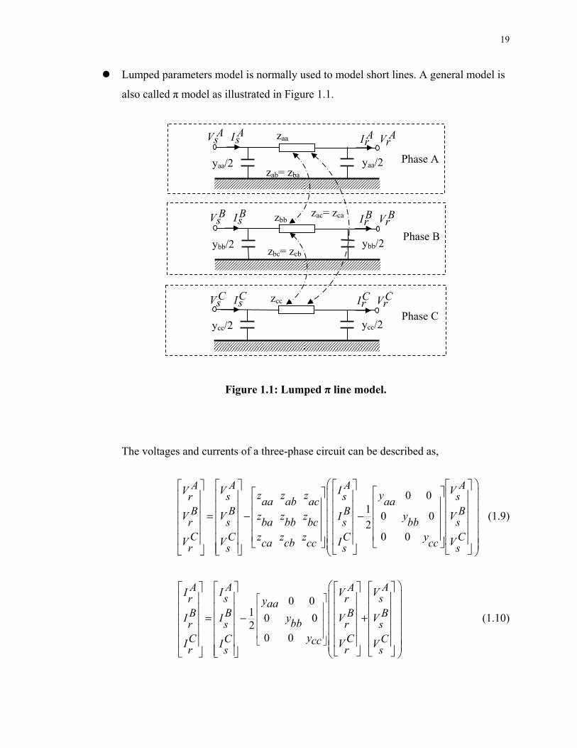
19
Lumped parameters model is normally used to model short lines. A general model is
also called π model as illustrated in Figure 1.1.
Figure 1.1: Lumped π line model.
The voltages and currents of a three-phase circuit can be described as,
0 01
0 02
0 0
A A AA V I VV z z z ys s sr aa ab ac aaB B B BV V z z z I y Vr s ba bb bc s bb sC C z z z C y CV V I Vca cb cc ccr s s s
= − −
(1.9)
0 01 0 02
0 0
A AA AI VI Vs sr ryaaB B B BI I y V Vbbr s r s
yC CC CccI VI Vr rs s
= − +
(1.10)
Phase A yaa/2 yaa/2
zaa
Phase B ybb/2 ybb/2
zbb
Phase C ycc/2 ycc/2
zcc
zab= zba
zbc= zcb
zac= zca
A AV Is s A AI Vr r
B BI Vr rB BV Is s
C CV Is sC CI Vr r
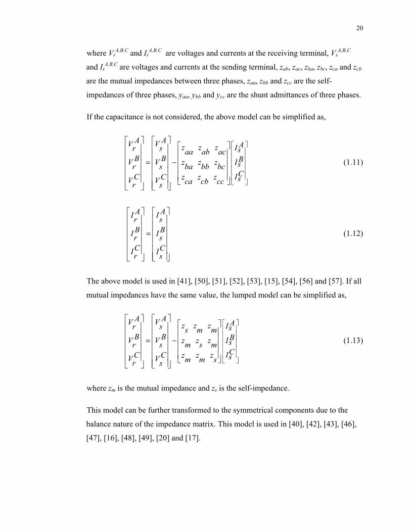
20
where VrA,B,C and Ir
A,B,C are voltages and currents at the receiving terminal, VsA,B,C
and IsA,B,C are voltages and currents at the sending terminal, zab, zac, zba, zbc, zca and zcb
are the mutual impedances between three phases, zaa, zbb and zcc are the self-
impedances of three phases, yaa, ybb and ycc are the shunt admittances of three phases.
If the capacitance is not considered, the above model can be simplified as,
AA VV Az z z Isr saa ab acB B BV V z z z Isr s ba bb bc
CIC C z z z sV V ca cb ccr s
= −
(1.11)
AA II srB BI Ir sC CI Ir s
=
(1.12)
The above model is used in [41], [50], [51], [52], [53], [15], [54], [56] and [57]. If all
mutual impedances have the same value, the lumped model can be simplified as,
AA VV Az z z Isr ss m mB B BV V z z z Isr s m s m
CIC C z z z sV V m m sr s
= −
(1.13)
where zm is the mutual impedance and zs is the self-impedance.
This model can be further transformed to the symmetrical components due to the
balance nature of the impedance matrix. This model is used in [40], [42], [43], [46],
[47], [16], [48], [49], [20] and [17].
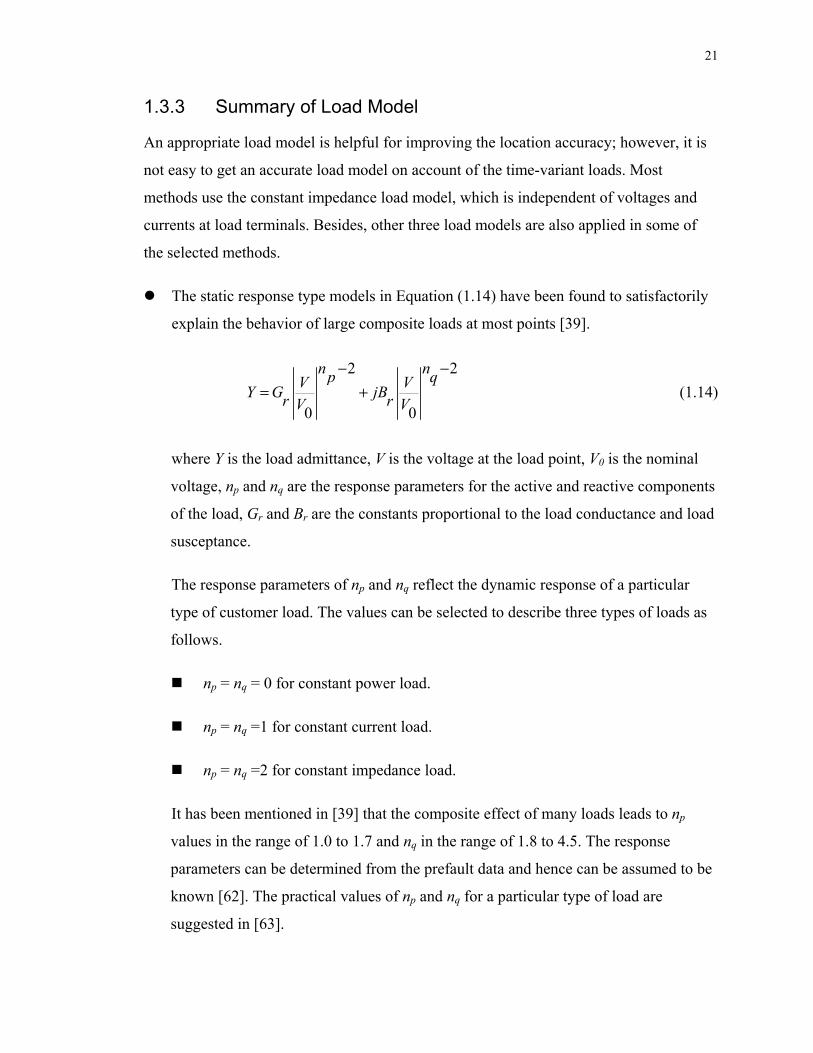
21
1.3.3 Summary of Load Model
An appropriate load model is helpful for improving the location accuracy; however, it is
not easy to get an accurate load model on account of the time-variant loads. Most
methods use the constant impedance load model, which is independent of voltages and
currents at load terminals. Besides, other three load models are also applied in some of
the selected methods.
The static response type models in Equation (1.14) have been found to satisfactorily
explain the behavior of large composite loads at most points [39].
2 2
0 0
n np qV VY G jBr rV V
− −= + (1.14)
where Y is the load admittance, V is the voltage at the load point, V0 is the nominal
voltage, np and nq are the response parameters for the active and reactive components
of the load, Gr and Br are the constants proportional to the load conductance and load
susceptance.
The response parameters of np and nq reflect the dynamic response of a particular
type of customer load. The values can be selected to describe three types of loads as
follows.
np = nq = 0 for constant power load.
np = nq =1 for constant current load.
np = nq =2 for constant impedance load.
It has been mentioned in [39] that the composite effect of many loads leads to np
values in the range of 1.0 to 1.7 and nq in the range of 1.8 to 4.5. The response
parameters can be determined from the prefault data and hence can be assumed to be
known [62]. The practical values of np and nq for a particular type of load are
suggested in [63].
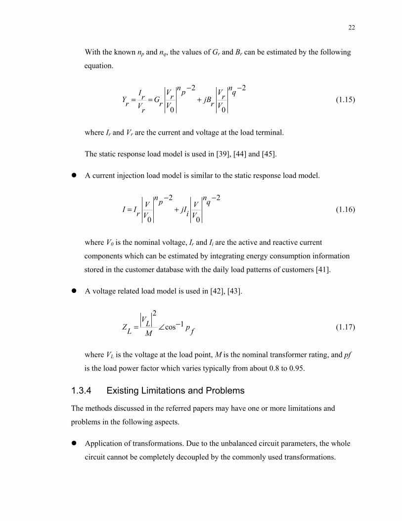
22
With the known np and nq, the values of Gr and Br can be estimated by the following
equation.
2 2
0 0
n np qV VI r rrY G jBr r rV VVr
− −= = + (1.15)
where Ir and Vr are the current and voltage at the load terminal.
The static response load model is used in [39], [44] and [45].
A current injection load model is similar to the static response load model.
2 2
0 0
n np qV VI I jIr iV V
− −= + (1.16)
where V0 is the nominal voltage, Ir and Ii are the active and reactive current
components which can be estimated by integrating energy consumption information
stored in the customer database with the daily load patterns of customers [41].
A voltage related load model is used in [42], [43].
2
1cosVLZ pL fM
−= ∠ (1.17)
where VL is the voltage at the load point, M is the nominal transformer rating, and pf
is the load power factor which varies typically from about 0.8 to 0.95.
1.3.4 Existing Limitations and Problems
The methods discussed in the referred papers may have one or more limitations and
problems in the following aspects.
Application of transformations. Due to the unbalanced circuit parameters, the whole
circuit cannot be completely decoupled by the commonly used transformations.
23
Presence of tap loads and laterals. The tap loads and/or laterals are not considered in
some fault location algorithms.
Heterogeneity of line sections. The heterogeneity of line sections is not considered in
some fault location algorithms.
Untransposed line. Most line and cable sections in a typical distribution network are
not ideally transposed so that the usage of symmetrical components is not proper.
Applications for underground cables. Most methods are applied for overhead lines in
distribution systems. However, only very few papers discuss the applications for
underground cables in distribution systems. The possibility and functionality is not
discussed if the algorithms developed for overhead lines are applied in the cases of
underground cables.
Effect of capacitance. The capacitance in cables is relatively larger than that in lines,
which would affect the voltage and current along the cable circuit.
Effect of sheaths in cables. There exist the voltage and current in the metallic sheaths
surrounding the core conductors.
Effect of bonding methods. Five bonding methods are widely used, namely, single
point bonding at sending terminal (SPBS), single point bonding at receiving terminal
(SPBR), single point bonding at middle point (SPBM), solid bonding at both ends
(SBBE), and cross bonding (XB). None of the published location algorithms
considered all bonding situations.
Problem of the multiple estimations. The present algorithms may find multiple fault
points, which specially exist in the impedance-based location algorithms. In some
papers, the multiple estimated points are ranked by possibilities [51], limited by fault
indicators [44] and [45], or eliminated by the fault diagnosis techniques [41], [54]
and [56].
Estimation of loads. In order to ensure the accuracy and performance of the location
algorithms in distribution networks, the techniques of load estimation, power flow
24
analysis or state estimation have to be applied. The load information can be acquired
either by the power flow analysis or load estimation based on the real time
measurements and historical load profile [15], [41], [52] and [53] where the existing
analysis methods [58] and [59] are used, or by the scaling methods based on the real
time measurements, load flow files and/or nominal transformer ratings [44], [51] and
[56].
1.4 Distribution State Estimation Methods
The state estimation for distribution networks is an important application in the
distribution management system (DMS) to provide the essential information for
operation, management, control and planning in distribution networks. It also assists in
the fault location algorithms by providing the necessary information of load flows and
bus states (voltage magnitudes and phases).
The present distribution state estimation (DSE) methods are reviewed below since a DSE
algorithm is proposed for underground distribution networks in this work.
Usually, the weighted least squares (WLS) technique is employed. Wan et al. proposed
two WLS approaches to estimate loads in unbalanced power distribution networks [64],
[65]. One is the WLS load parameter method to solve the constrained optimization
problem where loads are treated as variables. The constrained optimization problem is
transformed into an unconstrained problem by the exterior penalty method. The loads and
voltages are estimated simultaneously. Incorporating the operating and loading
constraints, the other one is a constrained WLS distribution state estimation-based
method to estimate voltages by a constrained WLS DSE, then to estimate loads
sequentially based on the estimated voltages.
Baran et al. proposed a three-phase state estimation method based on the WLS method in
[66]. A two-stage algorithm is developed to overcome the observability problems
associated with the branch current magnitude measurements. Rather than using nodal
voltages as estimation variables, the branch currents are used as state variables in the
state estimation to solve the WLS problem [67], where the Jacobian matrix is well
25
conditioned and can be decoupled on a phase basis. This method was substantially
revised in [68] where a new algorithm with the constant gain matrix and a decoupled
form was developed.
The problem of load estimation was formulated as a weighted least absolute values
estimation problem and solved by WLS [69]. The Newton-Raphson approach is applied
to eliminate the nonlinear effect of power losses.
In addition to WLS methods, the modified conventional algorithms were also proposed.
Extending the work in [59], the custom-tailored Gauss-Seidel load flow analysis was
proposed in [70]. A computationally efficient solution scheme based on the Newton-
Raphson method was proposed in [71]. An algorithm was developed to build a constant
Jacobian matrix [72] and the Newton-Raphson algorithm was also used to solve the load
flow problem.
The load flow problem of a radial distribution system was formulated as a convex
optimization problem, particularly a conic quadratic program [73]. The solution of the
distribution load flow problem can be obtained in polynomial time using interior-point
methods.
1.5 Objectives of the Thesis
The following objectives are proposed to be achieved during the course of this thesis:
Design of the incipient fault detection scheme for distribution cables;
Development of the fault location scheme for a medium voltage cable with no
laterals;
Design of the state estimation algorithm for underground distribution networks;
Extension of the proposed location algorithm to underground distribution networks
with the aid of the proposed state estimation algorithm.

26
1.6 Contributions of the Thesis
The contributions of the thesis are summarized as follows:
A wavelet analysis-based method is developed to detect incipient faults in cables in
time and frequency domains, additionally, identify transient and fault types, remove
effect of noise and supervise almost entire cable circuit.
A simple and practical algorithm based on the analysis of superimposed components
and negative sequence is particularly designed to detect single-line-to-ground
incipient faults in cables. The fewer thresholds and less computation are required.
A two-layer π circuit is formulated and examined to approximate the behavior and
characteristic of a typical medium voltage cable.
A set of fault location algorithms are proposed for underground cables. The
characteristics of underground cables in real systems are comprehensively considered
and analyzed in the development of algorithms, such as the shunt capacitance,
metallic sheath, heterogeneity and untranspositon. The cable configurations and fault
scenarios are taken into account as well, such as five bonding methods and three fault
pathways. Besides, a large number of fault equations are solved effectively and
efficiently and the fault resistance can be calculated.
The state estimation for underground distribution networks is formulated as a
nonlinear optimization problem and solved by the sequential quadratic programming
technique. The characteristics and configurations of underground cables and
distribution networks are considered in the development of the algorithm, such as the
shunt capacitance, metallic sheath, bonding method, unbalance loads and presence of
laterals and tapped loads.
A section-by-section estimation algorithm combined with the backward/forward
sweep algorithm is presented to estimate the nodal voltage and branch current for
each circuit section in a distribution network with laterals and tapped loads.
27
The combination of the fault location and state estimation algorithms is proposed to
solve the fault location problem in distribution cables.
The faulty section in distribution networks can be determined and the problem of
multiple estimations is eliminated.
Only the fundamental voltage and current phasors recorded at the single-end are
utilized in the proposed fault location and state estimation methods.
The performance and functionalities of the all proposed algorithms are examined and
verified with the extensive simulations, considering various fault conditions and
system configurations.
1.7 Scope of the Thesis
The thesis is organized in five chapters and two appendices. The first chapter outlines and
compares the present methods in the fields of incipient fault detection for cables, fault
location for cables, fault location for distribution networks and state estimation for
distribution networks. The objectives, contributions and scope of the thesis are introduced
and summarized as well.
Chapter 2 describes the development of the incipient fault detection algorithms for
distribution cables. The basic concept of incipient faults in cables is first introduced and
the model of arc is formulated. Then two algorithms are proposed, one is based on the
wavelet analysis and the other is based on the analysis of the superimposed fault current
and negative sequence current in time domain. Two test distribution systems, extensive
simulation cases and field cases are investigated.
Chapter 3 focuses on proposing a set of fault location algorithms for underground
medium voltage cables with no laterals. First, a series of the basic background knowledge
is introduced. Then the principle and procedure of the location algorithms are specially
explicated for a cable with sheaths grounded at the sending terminal. The differences and
similarities of the algorithms for other bonding methods are compared and summarized as
well. The estimation of constant load impedance is explained and the application of the

28
static response load model is also discussed. The extensive simulations are carried out
and explained to demonstrate the accuracy and effectiveness of the proposed algorithms.
Chapter 4 is to extend the proposed fault location algorithms to underground distribution
networks. Since the distribution state estimation is capable of providing the additional
information for the fault location algorithms, this chapter includes two parts:
development of a state estimation algorithm for underground distribution networks and
extension of the proposed location algorithms to underground distribution networks with
the aid of the proposed state estimation algorithm. The basic background knowledge is
first introduced and the details of the proposed state estimation algorithm are discussed.
Then a general location procedure combined with the state estimation is described as
well. The algorithms are examined on a radial underground distribution network with
different load and fault conditions.
Chapter 5 presents the conclusions and the suggested future works, followed by the list of
references.
Appendices describe the supplement document and additional work performed during the
course of this research. An example of traveling waves is illustrated in a spatiotemporal
domain to demonstrate a clear process of the propagation and reflection of traveling
waves in a transmission line. The voltage, current and resistance of an arc are also
illustrated.
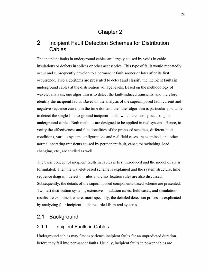
29
Chapter 2
2 Incipient Fault Detection Schemes for Distribution Cables
The incipient faults in underground cables are largely caused by voids in cable
insulations or defects in splices or other accessories. This type of fault would repeatedly
occur and subsequently develop to a permanent fault sooner or later after its first
occurrence. Two algorithms are presented to detect and classify the incipient faults in
underground cables at the distribution voltage levels. Based on the methodology of
wavelet analysis, one algorithm is to detect the fault-induced transients, and therefore
identify the incipient faults. Based on the analysis of the superimposed fault current and
negative sequence current in the time domain, the other algorithm is particularly suitable
to detect the single-line-to-ground incipient faults, which are mostly occurring in
underground cables. Both methods are designed to be applied in real systems. Hence, to
verify the effectiveness and functionalities of the proposed schemes, different fault
conditions, various system configurations and real field cases are examined, and other
normal operating transients caused by permanent fault, capacitor switching, load
changing, etc., are studied as well.
The basic concept of incipient faults in cables is first introduced and the model of arc is
formulated. Then the wavelet-based scheme is explained and the system structure, time
sequence diagram, detection rules and classification rules are also discussed.
Subsequently, the details of the superimposed components-based scheme are presented.
Two test distribution systems, extensive simulation cases, field cases, and simulation
results are examined, where, more specially, the detailed detection process is explicated
by analyzing four incipient faults recorded from real systems.
2.1 Background
2.1.1 Incipient Faults in Cables
Underground cables may first experience incipient faults for an unpredicted duration
before they fail into permanent faults. Usually, incipient faults in power cables are
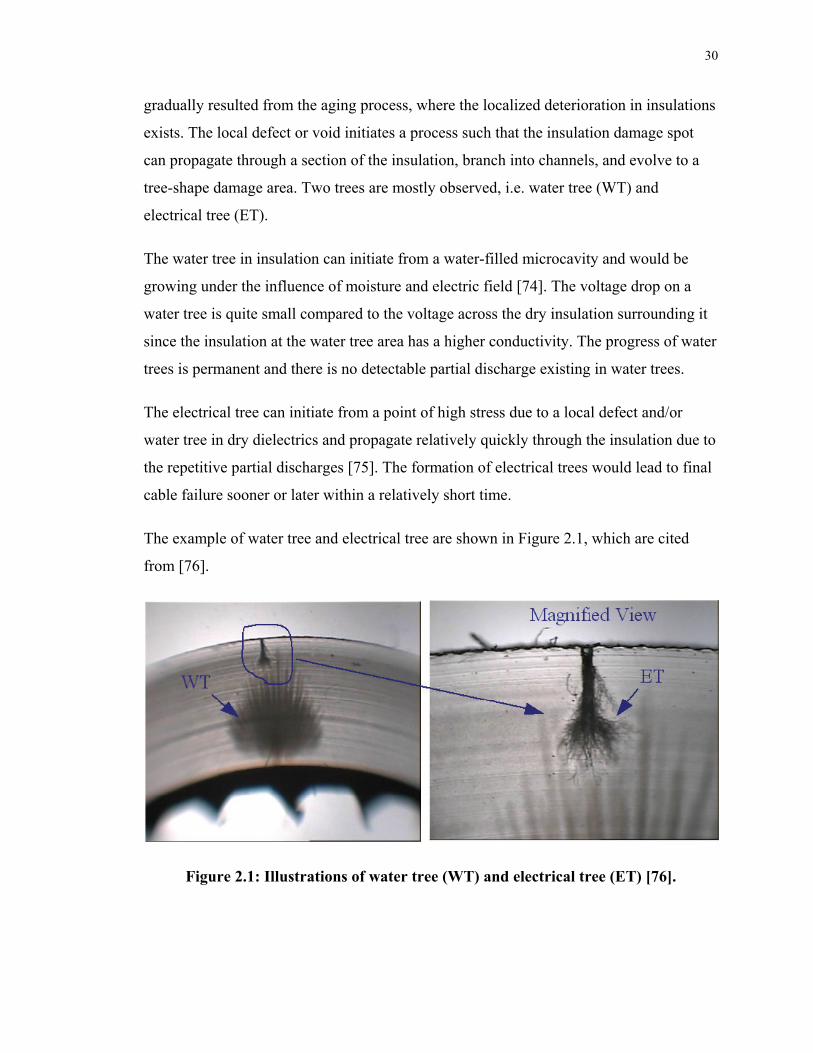
30
gradually resulted from the aging process, where the localized deterioration in insulations
exists. The local defect or void initiates a process such that the insulation damage spot
can propagate through a section of the insulation, branch into channels, and evolve to a
tree-shape damage area. Two trees are mostly observed, i.e. water tree (WT) and
electrical tree (ET).
The water tree in insulation can initiate from a water-filled microcavity and would be
growing under the influence of moisture and electric field [74]. The voltage drop on a
water tree is quite small compared to the voltage across the dry insulation surrounding it
since the insulation at the water tree area has a higher conductivity. The progress of water
trees is permanent and there is no detectable partial discharge existing in water trees.
The electrical tree can initiate from a point of high stress due to a local defect and/or
water tree in dry dielectrics and propagate relatively quickly through the insulation due to
the repetitive partial discharges [75]. The formation of electrical trees would lead to final
cable failure sooner or later within a relatively short time.
The example of water tree and electrical tree are shown in Figure 2.1, which are cited
from [76].
Figure 2.1: Illustrations of water tree (WT) and electrical tree (ET) [76].

31
Overall, electrical overstress in conjunction with mechanical deficiency, unfavorable
environmental condition, and chemical pollution, can cause the irreparable and
irreversible damages in insulations. The details of the inception of aging and propagation
mechanisms are explained in [77].
The formation of electrical trees would generate partial discharges, which can be
considered as the early stage of incipient faults before the condition of insulation gets
worse. The partial discharge is characterized by a series of short discharge current pulses
with the width of about one nanosecond and with the time interval of several tens of
nanoseconds between successive discharges. Therefore, the detection of early cable
defects or failures can be classified into two categories: detection of partial discharges
and detection of incipient faults. Both of them are concerned by the utility companies,
and the power protection engineers would pay more attention on the latter one. The
proposed method is also directly associated with the latter one.
Incipient faults are normally characterized as the faulty phenomena with the relatively
low fault currents and the relatively short duration ranging from one-quarter cycle to
multi-cycle. These short lasting current variations cannot be detected by the traditional
distribution protection schemes because of their short duration and low increment in
magnitude. However, such faults must be detected at the early stage to avoid the
consequent catastrophe induced by the degradation themselves. The field experience and
laboratory experiments of incipient faults are investigated in [78], [79].
In underground cables, the incipient fault is one type of transients in power systems,
which is prone to an intermittent arc fault. The typical incipient faults are composed of
two types: sub-cycle incipient fault and multi-cycle incipient fault. The sub-cycle
incipient fault always occurs near a voltage peak where arc is ignited, lasts around one-
quarter cycle, and self-clears when the current crosses zero. Figure 2.2 shows the three-
phase feeder currents when a sub-cycle incipient fault occurs between phase A and
ground at the 2 km location of a 9 km cable in the first test system in Section 2.4.2. The
multi-cycle incipient fault also likely occurs near a voltage peak, lasts 1-4 cycles, and
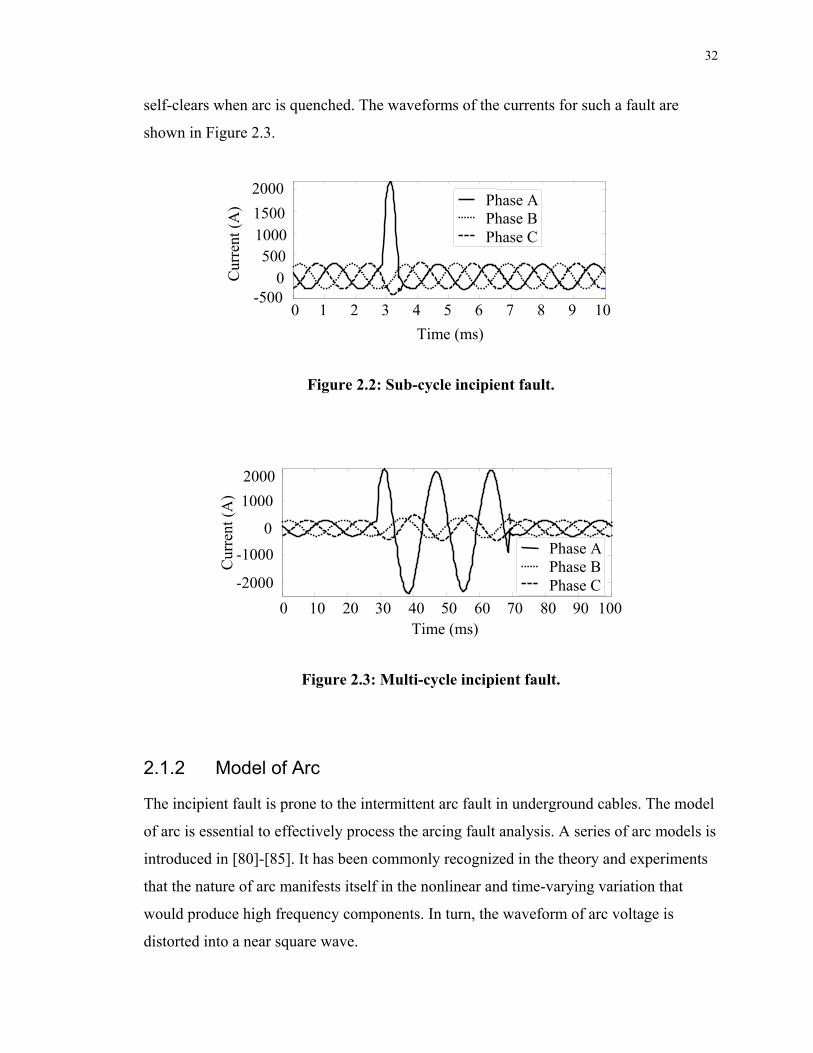
32
self-clears when arc is quenched. The waveforms of the currents for such a fault are
shown in Figure 2.3.
Figure 2.2: Sub-cycle incipient fault.
Figure 2.3: Multi-cycle incipient fault.
2.1.2 Model of Arc
The incipient fault is prone to the intermittent arc fault in underground cables. The model
of arc is essential to effectively process the arcing fault analysis. A series of arc models is
introduced in [80]-[85]. It has been commonly recognized in the theory and experiments
that the nature of arc manifests itself in the nonlinear and time-varying variation that
would produce high frequency components. In turn, the waveform of arc voltage is
distorted into a near square wave.
0 1 2 3 4 5 6 7 8 9 10-500
0 500
1000 1500
2000
Time (ms)
Phase A Phase B Phase C
Cur
rent
(A
)
0 10 20 30 40 50 60 70 80 90 100
-2000
-1000
0
1000
2000
Cur
rent
(A
)
Time (ms)
Phase A Phase B Phase C
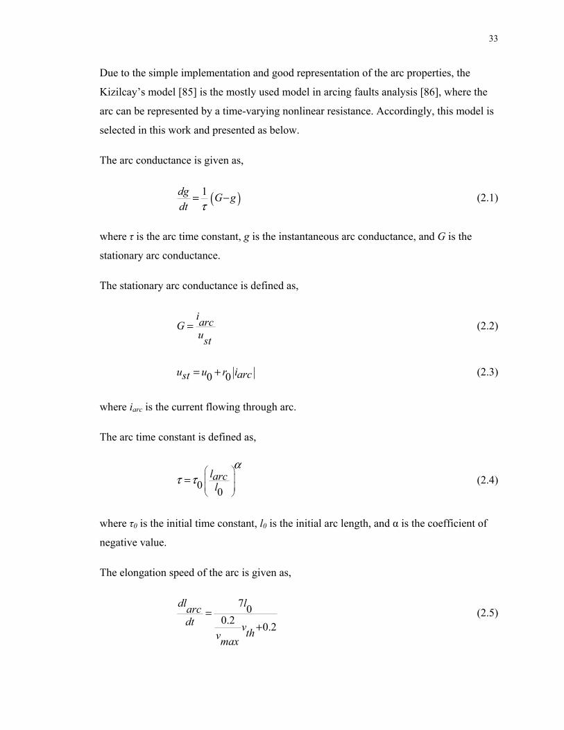
33
Due to the simple implementation and good representation of the arc properties, the
Kizilcay’s model [85] is the mostly used model in arcing faults analysis [86], where the
arc can be represented by a time-varying nonlinear resistance. Accordingly, this model is
selected in this work and presented as below.
The arc conductance is given as,
( )1dgG g
dt τ= − (2.1)
where τ is the arc time constant, g is the instantaneous arc conductance, and G is the
stationary arc conductance.
The stationary arc conductance is defined as,
iarcGust
= (2.2)
0 0u u r iarcst = + (2.3)
where iarc is the current flowing through arc.
The arc time constant is defined as,
00
larcl
ατ τ
= (2.4)
where τ0 is the initial time constant, l0 is the initial arc length, and α is the coefficient of
negative value.
The elongation speed of the arc is given as,
7 00.2
0.2
dl larcdt vthvmax
=+
(2.5)
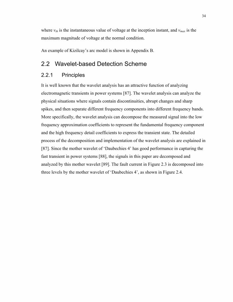
34
where vth is the instantaneous value of voltage at the inception instant, and vmax is the
maximum magnitude of voltage at the normal condition.
An example of Kizilcay’s arc model is shown in Appendix B.
2.2 Wavelet-based Detection Scheme
2.2.1 Principles
It is well known that the wavelet analysis has an attractive function of analyzing
electromagnetic transients in power systems [87]. The wavelet analysis can analyze the
physical situations where signals contain discontinuities, abrupt changes and sharp
spikes, and then separate different frequency components into different frequency bands.
More specifically, the wavelet analysis can decompose the measured signal into the low
frequency approximation coefficients to represent the fundamental frequency component
and the high frequency detail coefficients to express the transient state. The detailed
process of the decomposition and implementation of the wavelet analysis are explained in
[87]. Since the mother wavelet of ‘Daubechies 4’ has good performance in capturing the
fast transient in power systems [88], the signals in this paper are decomposed and
analyzed by this mother wavelet [89]. The fault current in Figure 2.3 is decomposed into
three levels by the mother wavelet of ‘Daubechies 4’, as shown in Figure 2.4.
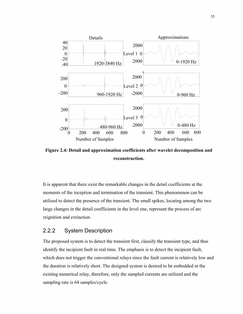
35
Figure 2.4: Detail and approximation coefficients after wavelet decomposition and
reconstruction.
It is apparent that there exist the remarkable changes in the detail coefficients at the
moments of the inception and termination of the transient. This phenomenon can be
utilized to detect the presence of the transient. The small spikes, locating among the two
large changes in the detail coefficients in the level one, represent the process of arc
reignition and extinction.
2.2.2 System Description
The proposed system is to detect the transient first, classify the transient type, and thus
identify the incipient fault in real time. The emphasis is to detect the incipient fault,
which does not trigger the conventional relays since the fault current is relatively low and
the duration is relatively short. The designed system is desired to be embedded in the
existing numerical relay, therefore, only the sampled currents are utilized and the
sampling rate is 64 samples/cycle.
-40 -20
0 20 40
Details
0
-2000
0
2000
Approximations
-200
0
200
-2000
0
2000
0 200 400 600 800-200
0
200
0 200 400 600 800
-2000
0
2000
Level 1
Level 2
Level 3
1920-3840 Hz
960-1920 Hz
480-960 Hz
0-1920 Hz
0-960 Hz
0-480 Hz
Number of Samples Number of Samples
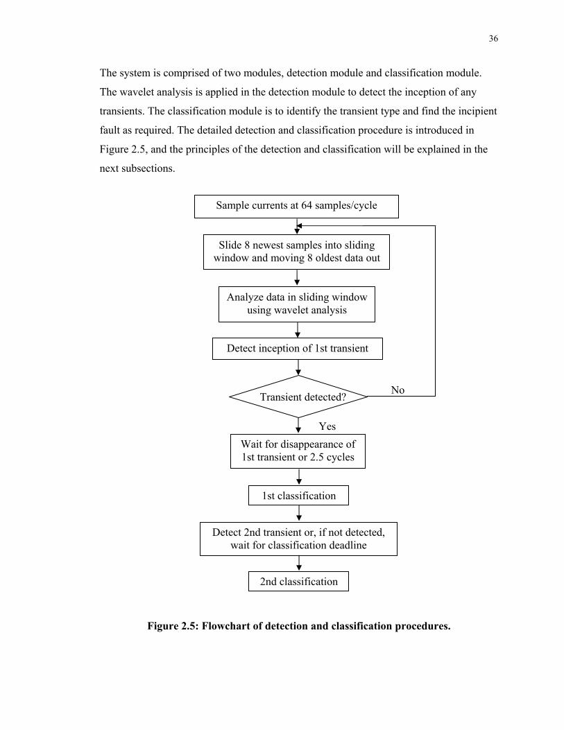
36
The system is comprised of two modules, detection module and classification module.
The wavelet analysis is applied in the detection module to detect the inception of any
transients. The classification module is to identify the transient type and find the incipient
fault as required. The detailed detection and classification procedure is introduced in
Figure 2.5, and the principles of the detection and classification will be explained in the
next subsections.
Figure 2.5: Flowchart of detection and classification procedures.
Sample currents at 64 samples/cycle
Slide 8 newest samples into sliding window and moving 8 oldest data out
Analyze data in sliding window using wavelet analysis
Detect inception of 1st transient
Transient detected?
Wait for disappearance of 1st transient or 2.5 cycles
1st classification
Detect 2nd transient or, if not detected, wait for classification deadline
2nd classification
Yes
No
37
The detection module includes two detection steps. The first step is to detect the
inception of transient, and the second is to recognize the possible subsequent transient,
such as the breaker operation, end of incipient fault, and arc quench, etc.
The classification module also includes two steps. The first step is to pre-classify the
transient type at the moment of the disappearance of the first transient or 2.5 cycles later
than the inception of the first transient. This pre-classified result is not definitely correct
because some events may have the similar initial transient phenomena after the
occurrence of the first transient. Hence, the second classification is applied to revise the
previous result at the moment of the disappearance of the second detected transient or at
the moment of the preset deadline time. Usually, the deadline time can be set up as 4 or 5
cycles after the first transient is detected.
The time sequence diagram of the detection and classification procedures is shown in
Figure 2.6. Two examples are illustrated in Figure 2.7 and Figure 2.8 to give a more
visualized demonstration.
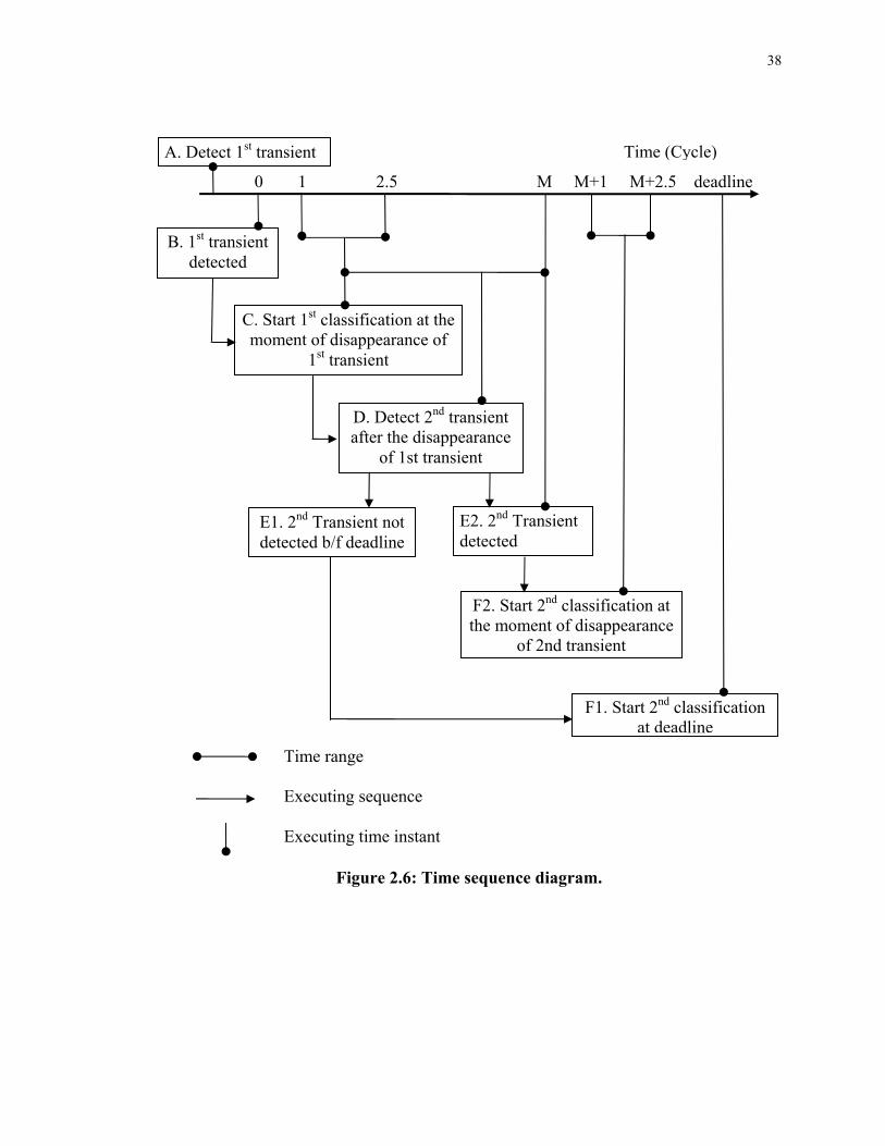
38
Figure 2.6: Time sequence diagram.
B. 1st transient detected
0 1 2.5 M M+1 M+2.5 deadline
C. Start 1st classification at the moment of disappearance of
1st transient
F1. Start 2nd classification at deadline
D. Detect 2nd transient after the disappearance
of 1st transient
E1. 2nd Transient not detected b/f deadline
Time (Cycle)
F2. Start 2nd classification at the moment of disappearance
of 2nd transient
E2. 2nd Transient detected
Time range Executing sequence Executing time instant
A. Detect 1st transient
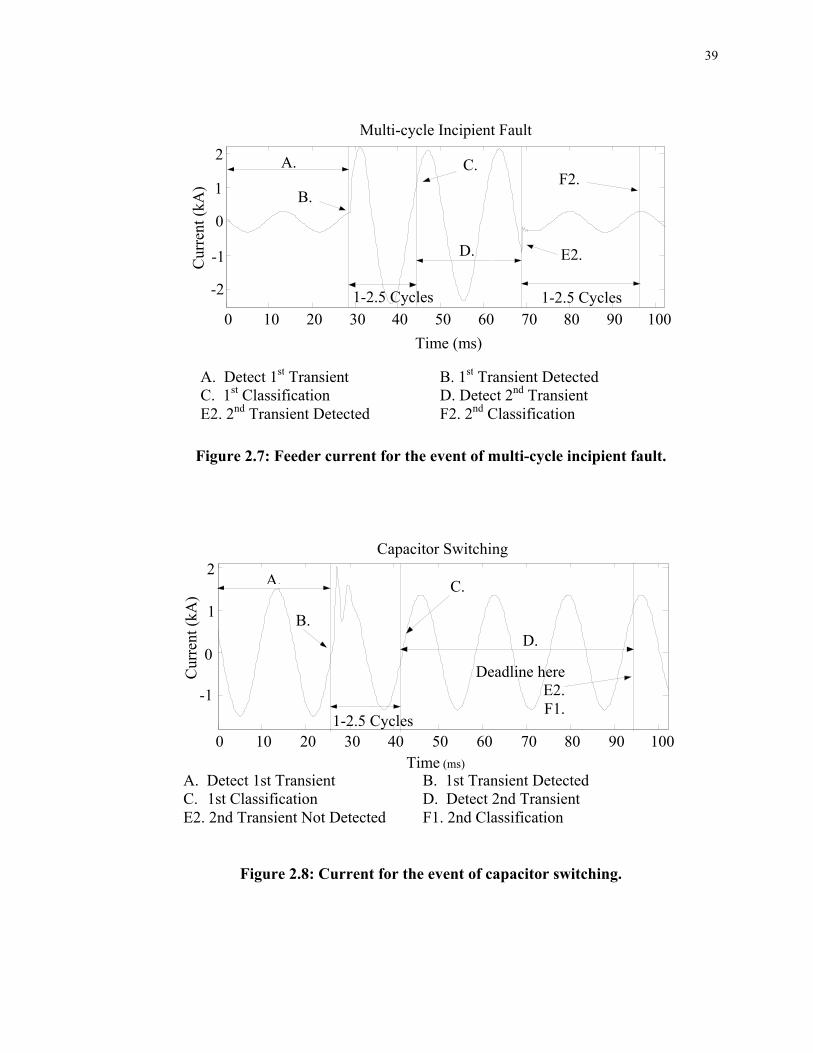
39
Figure 2.7: Feeder current for the event of multi-cycle incipient fault.
Figure 2.8: Current for the event of capacitor switching.
0 10 20 30 40 50 60 70 80 90 100
-2
-1
0
1
2
Multi-cycle Incipient Fault
Time (ms)
Cur
rent
(kA
)
1-2.5 Cycles
A.
B.
C.
1-2.5 Cycles
D.
F2.
E2.
A. Detect 1st Transient B. 1st Transient Detected C. 1st Classification D. Detect 2nd Transient E2. 2nd Transient Detected F2. 2nd Classification
0 10 20 30 40 50 60 70 80 90 100
-1
0
1
2 Capacitor Switching
Time (ms)
1-2.5 Cycles
Cur
rent
(kA
)
A.
B.
C.
D.
Deadline hereE2. F1.
A. Detect 1st Transient B. 1st Transient Detected C. 1st Classification D. Detect 2nd Transient E2. 2nd Transient Not Detected F1. 2nd Classification
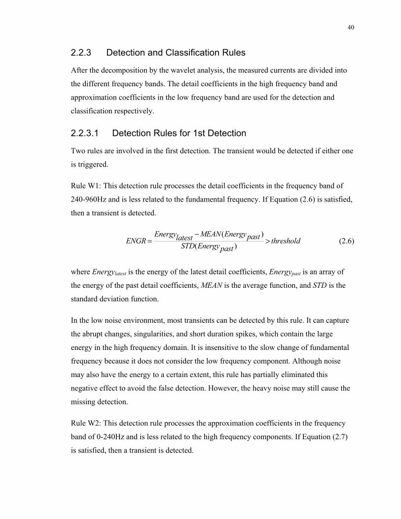
40
2.2.3 Detection and Classification Rules
After the decomposition by the wavelet analysis, the measured currents are divided into
the different frequency bands. The detail coefficients in the high frequency band and
approximation coefficients in the low frequency band are used for the detection and
classification respectively.
2.2.3.1 Detection Rules for 1st Detection
Two rules are involved in the first detection. The transient would be detected if either one
is triggered.
Rule W1: This detection rule processes the detail coefficients in the frequency band of
240-960Hz and is less related to the fundamental frequency. If Equation (2.6) is satisfied,
then a transient is detected.
( )
( )
Energy MEAN EnergypastlatestENGR thresholdSTD Energypast
−= > (2.6)
where Energylatest is the energy of the latest detail coefficients, Energypast is an array of
the energy of the past detail coefficients, MEAN is the average function, and STD is the
standard deviation function.
In the low noise environment, most transients can be detected by this rule. It can capture
the abrupt changes, singularities, and short duration spikes, which contain the large
energy in the high frequency domain. It is insensitive to the slow change of fundamental
frequency because it does not consider the low frequency component. Although noise
may also have the energy to a certain extent, this rule has partially eliminated this
negative effect to avoid the false detection. However, the heavy noise may still cause the
missing detection.
Rule W2: This detection rule processes the approximation coefficients in the frequency
band of 0-240Hz and is less related to the high frequency components. If Equation (2.7)
is satisfied, then a transient is detected.
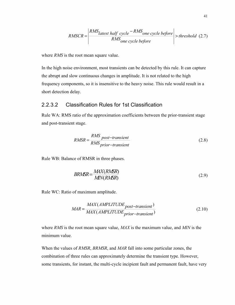
41
RMS RMSlatest half cycle one cycle beforeRMSCR threshold
RMSone cycle before
−= > (2.7)
where RMS is the root mean square value.
In the high noise environment, most transients can be detected by this rule. It can capture
the abrupt and slow continuous changes in amplitude. It is not related to the high
frequency components, so it is insensitive to the heavy noise. This rule would result in a
short detection delay.
2.2.3.2 Classification Rules for 1st Classification
Rule WA: RMS ratio of the approximation coefficients between the prior-transient stage
and post-transient stage.
RMS post transientRMSRRMS prior transient
−=−
(2.8)
Rule WB: Balance of RMSR in three phases.
( )( )
MAX RMSRBRMSRMIN RMSR
= (2.9)
Rule WC: Ratio of maximum amplitude.
( )
( )
MAX AMPLITUDEpost transientMARMAX AMPLITUDEprior transient
−=−
(2.10)
where RMS is the root mean square value, MAX is the maximum value, and MIN is the
minimum value.
When the values of RMSR, BRMSR, and MAR fall into some particular zones, the
combination of three rules can approximately determine the transient type. However,
some transients, for instant, the multi-cycle incipient fault and permanent fault, have very
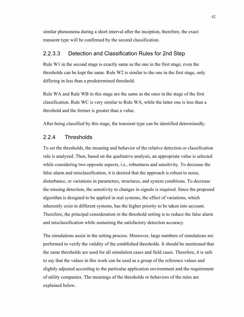
42
similar phenomena during a short interval after the inception, therefore, the exact
transient type will be confirmed by the second classification.
2.2.3.3 Detection and Classification Rules for 2nd Step
Rule W1 in the second stage is exactly same as the one in the first stage, even the
thresholds can be kept the same. Rule W2 is similar to the one in the first stage, only
differing in less than a predetermined threshold.
Rule WA and Rule WB in this stage are the same as the ones in the stage of the first
classification. Rule WC is very similar to Rule WA, while the latter one is less than a
threshold and the former is greater than a value.
After being classified by this stage, the transient type can be identified determinedly.
2.2.4 Thresholds
To set the thresholds, the meaning and behavior of the relative detection or classification
rule is analyzed. Then, based on the qualitative analysis, an appropriate value is selected
while considering two opposite aspects, i.e., robustness and sensitivity. To decrease the
false alarm and misclassification, it is desired that the approach is robust to noise,
disturbance, or variations in parameters, structures, and system conditions. To decrease
the missing detection, the sensitivity to changes in signals is required. Since the proposed
algorithm is designed to be applied in real systems, the effect of variations, which
inherently exist in different systems, has the higher priority to be taken into account.
Therefore, the principal consideration in the threshold setting is to reduce the false alarm
and misclassification while sustaining the satisfactory detection accuracy.
The simulations assist in the setting process. Moreover, large numbers of simulations are
performed to verify the validity of the established thresholds. It should be mentioned that
the same thresholds are used for all simulation cases and field cases. Therefore, it is safe
to say that the values in this work can be used as a group of the reference values and
slightly adjusted according to the particular application environment and the requirement
of utility companies. The meanings of the thresholds or behaviors of the rules are
explained below.
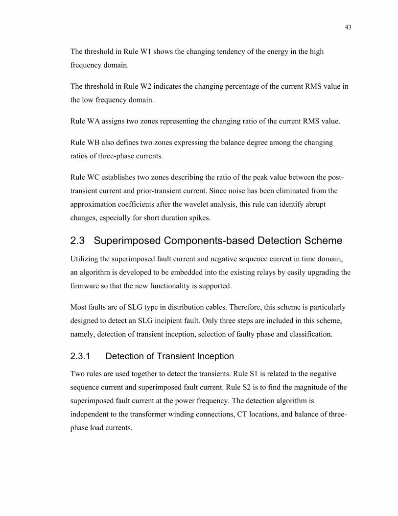
43
The threshold in Rule W1 shows the changing tendency of the energy in the high
frequency domain.
The threshold in Rule W2 indicates the changing percentage of the current RMS value in
the low frequency domain.
Rule WA assigns two zones representing the changing ratio of the current RMS value.
Rule WB also defines two zones expressing the balance degree among the changing
ratios of three-phase currents.
Rule WC establishes two zones describing the ratio of the peak value between the post-
transient current and prior-transient current. Since noise has been eliminated from the
approximation coefficients after the wavelet analysis, this rule can identify abrupt
changes, especially for short duration spikes.
2.3 Superimposed Components-based Detection Scheme
Utilizing the superimposed fault current and negative sequence current in time domain,
an algorithm is developed to be embedded into the existing relays by easily upgrading the
firmware so that the new functionality is supported.
Most faults are of SLG type in distribution cables. Therefore, this scheme is particularly
designed to detect an SLG incipient fault. Only three steps are included in this scheme,
namely, detection of transient inception, selection of faulty phase and classification.
2.3.1 Detection of Transient Inception
Two rules are used together to detect the transients. Rule S1 is related to the negative
sequence current and superimposed fault current. Rule S2 is to find the magnitude of the
superimposed fault current at the power frequency. The detection algorithm is
independent to the transformer winding connections, CT locations, and balance of three-
phase load currents.
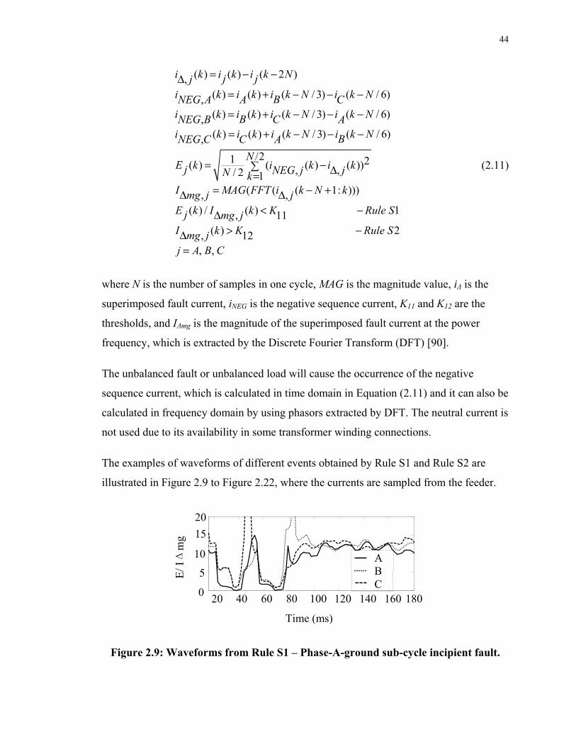
44
( ) ( ) ( 2 ),( ) ( ) ( / 3) ( / 6),( ) ( ) ( / 3) ( / 6),( ) ( ) ( / 3) ( / 6),
/21 2( ) ( ( ) ( )),,/ 2 1( ( ( 1: ))), ,
( ) /
i k i k i k Nj jji k i k i k N i k NBNEG A A Ci k i k i k N i k NBNEG B C Ai k i k i k N i k NBNEG C C A
NE k i k i kj jNEG jN kI MAG FFT i k N kmg j jE kj
= − −Δ= + − − −
= + − − −
= + − − −
= − Δ== − +Δ Δ
( ) 1, 11( ) 2, 12
, ,
I k K Rule Smg jI k K Rule Smg jj A B C
< −Δ> −Δ
=
(2.11)
where N is the number of samples in one cycle, MAG is the magnitude value, iΔ is the
superimposed fault current, iNEG is the negative sequence current, K11 and K12 are the
thresholds, and IΔmg is the magnitude of the superimposed fault current at the power
frequency, which is extracted by the Discrete Fourier Transform (DFT) [90].
The unbalanced fault or unbalanced load will cause the occurrence of the negative
sequence current, which is calculated in time domain in Equation (2.11) and it can also be
calculated in frequency domain by using phasors extracted by DFT. The neutral current is
not used due to its availability in some transformer winding connections.
The examples of waveforms of different events obtained by Rule S1 and Rule S2 are
illustrated in Figure 2.9 to Figure 2.22, where the currents are sampled from the feeder.
Figure 2.9: Waveforms from Rule S1 – Phase-A-ground sub-cycle incipient fault.
20 40 60 80 100 120 140 160 180 0
5
10
15
20
Time (ms)
A B C
E/ IΔ
mg
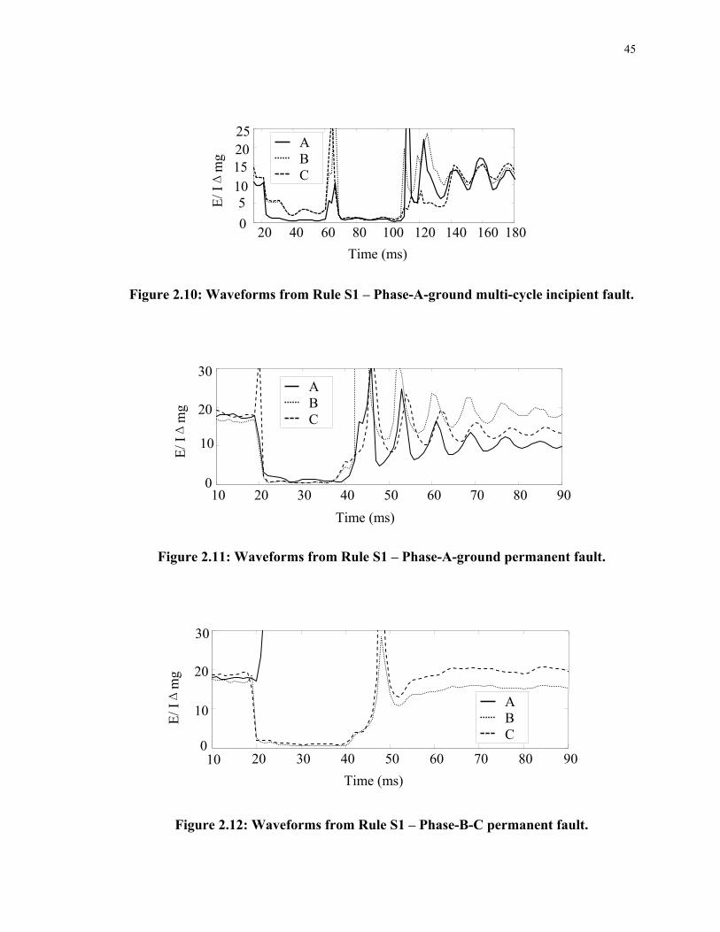
45
Figure 2.10: Waveforms from Rule S1 – Phase-A-ground multi-cycle incipient fault.
Figure 2.11: Waveforms from Rule S1 – Phase-A-ground permanent fault.
Figure 2.12: Waveforms from Rule S1 – Phase-B-C permanent fault.
20 40 60 80 100 120 140 160 180 0
5 10 15 20 25
Time (ms)
A B C
E/ IΔ
mg
10 20 30 40 50 60 70 80 90 0
10
20
30 A
B C
E/ IΔ
mg
Time (ms)
10 20 30 40 50 60 70 80 90 0
10
20
30
A B C
E/ IΔ
mg
Time (ms)
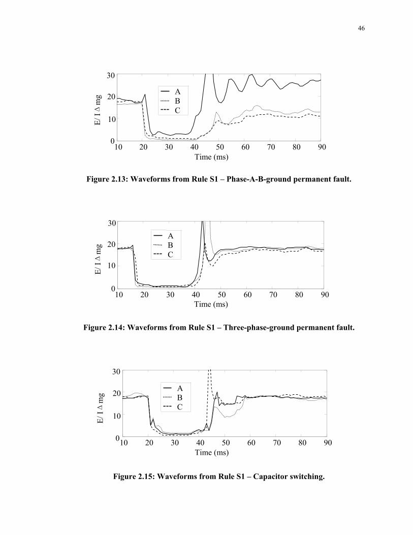
46
Figure 2.13: Waveforms from Rule S1 – Phase-A-B-ground permanent fault.
Figure 2.14: Waveforms from Rule S1 – Three-phase-ground permanent fault.
Figure 2.15: Waveforms from Rule S1 – Capacitor switching.
10 20 30 40 50 60 70 80 90 0
10
20
30
E/ IΔ
mg
Time (ms)
A B C
10 20 30 40 50 60 70 80 90 0
10
20
30
Time (ms)
E/ IΔ
mg
A B C
10 20 30 40 50 60 70 80 90 0
10
20
30
Time (ms)
E/ IΔ
mg
A B C
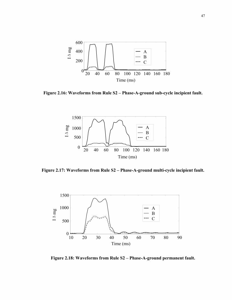
47
Figure 2.16: Waveforms from Rule S2 – Phase-A-ground sub-cycle incipient fault.
Figure 2.17: Waveforms from Rule S2 – Phase-A-ground multi-cycle incipient fault.
Figure 2.18: Waveforms from Rule S2 – Phase-A-ground permanent fault.
20 40 60 80 100 120 140 160 180 0
500
1000
1500
Time (ms)
A B C I
Δm
g
20 40 60 80 100 120 140 160 180 0
200
400
600
Time (ms)
A B C
IΔ
mg
10 20 30 40 50 60 70 80 90 0
500
1000
1500
IΔ
mg
Time (ms)
A B C
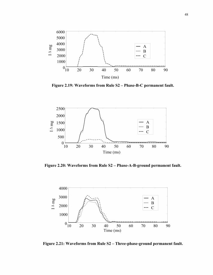
48
Figure 2.19: Waveforms from Rule S2 – Phase-B-C permanent fault.
Figure 2.20: Waveforms from Rule S2 – Phase-A-B-ground permanent fault.
Figure 2.21: Waveforms from Rule S2 – Three-phase-ground permanent fault.
10 20 30 40 50 60 70 80 90 0
1000
2000
3000
4000
5000
6000
A B C I
Δm
g
Time (ms)
10 20 30 40 50 60 70 80 90 0
500
1000
1500
2000
2500
A B C IΔ
mg
Time (ms)
10 20 30 40 50 60 70 80 90 0
1000
2000
3000
4000
A B C
Time (ms)
IΔ
mg
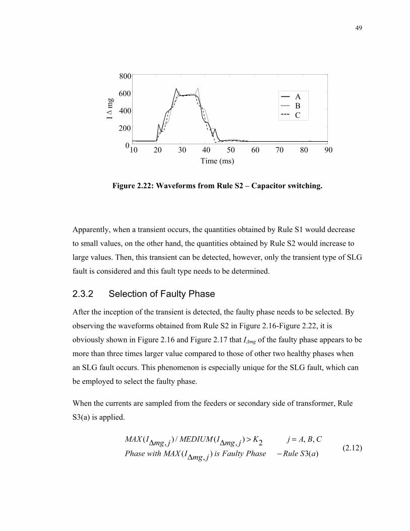
49
Figure 2.22: Waveforms from Rule S2 – Capacitor switching.
Apparently, when a transient occurs, the quantities obtained by Rule S1 would decrease
to small values, on the other hand, the quantities obtained by Rule S2 would increase to
large values. Then, this transient can be detected, however, only the transient type of SLG
fault is considered and this fault type needs to be determined.
2.3.2 Selection of Faulty Phase
After the inception of the transient is detected, the faulty phase needs to be selected. By
observing the waveforms obtained from Rule S2 in Figure 2.16-Figure 2.22, it is
obviously shown in Figure 2.16 and Figure 2.17 that IΔmg of the faulty phase appears to be
more than three times larger value compared to those of other two healthy phases when
an SLG fault occurs. This phenomenon is especially unique for the SLG fault, which can
be employed to select the faulty phase.
When the currents are sampled from the feeders or secondary side of transformer, Rule
S3(a) is applied.
( ) / ( ) , ,, , 2( ) 3( ),
MAX I MEDIUM I K j A B Cmg j mg jPhase with MAX I is Faulty Phase Rule S amg j
> =Δ Δ−Δ
(2.12)
10 20 30 40 50 60 70 80 900
200
400
600
800
IΔ
mg
Time (ms)
A B C
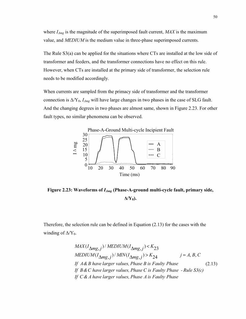
50
where IΔmg is the magnitude of the superimposed fault current, MAX is the maximum
value, and MEDIUM is the medium value in three-phase superimposed currents.
The Rule S3(a) can be applied for the situations where CTs are installed at the low side of
transformer and feeders, and the transformer connections have no effect on this rule.
However, when CTs are installed at the primary side of transformer, the selection rule
needs to be modified accordingly.
When currents are sampled from the primacy side of transformer and the transformer
connection is Δ/Y0, IΔmg will have large changes in two phases in the case of SLG fault.
And the changing degrees in two phases are almost same, shown in Figure 2.23. For other
fault types, no similar phenomena can be observed.
Figure 2.23: Waveforms of IΔmg (Phase-A-ground multi-cycle fault, primary side,
Δ/Y0).
Therefore, the selection rule can be defined in Equation (2.13) for the cases with the
winding of Δ/Y0.
( ) / ( ), , 23( ) / ( ) , ,, , 24
MAX I MEDIUM I Kmg j mg jMEDIUM I MIN I K j A B Cmg j mg jIf A& B have larger values, Phase B is Faulty PhaseIf B&C have larger values, Phase C is Faulty Phase - Rule S3(c)If C & A have larger values, Phase A is Faulty Phase
<Δ Δ> =Δ Δ
(2.13)
10 20 30 40 50 60 70 80 90 0 5
10 15 20 25 30
Phase-A-Ground Multi-cycle Incipient Fault
Time (ms)
A B C I
Δm
g
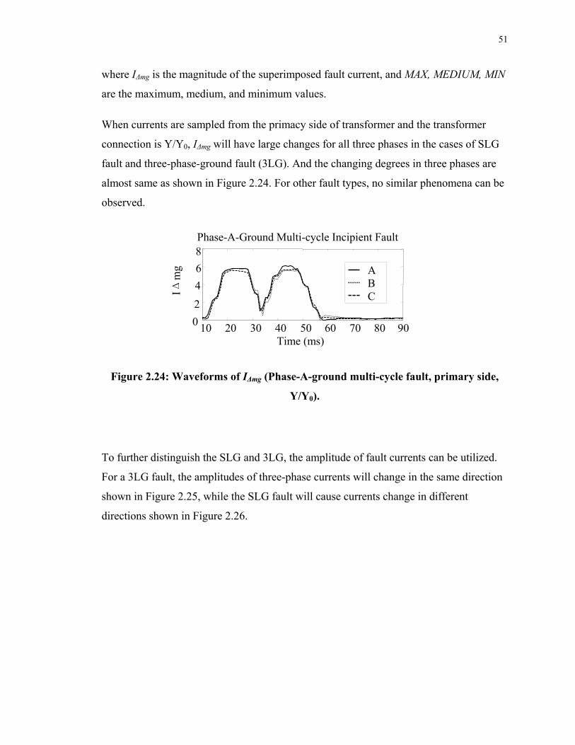
51
where IΔmg is the magnitude of the superimposed fault current, and MAX, MEDIUM, MIN
are the maximum, medium, and minimum values.
When currents are sampled from the primacy side of transformer and the transformer
connection is Y/Y0, IΔmg will have large changes for all three phases in the cases of SLG
fault and three-phase-ground fault (3LG). And the changing degrees in three phases are
almost same as shown in Figure 2.24. For other fault types, no similar phenomena can be
observed.
Figure 2.24: Waveforms of IΔmg (Phase-A-ground multi-cycle fault, primary side,
Y/Y0).
To further distinguish the SLG and 3LG, the amplitude of fault currents can be utilized.
For a 3LG fault, the amplitudes of three-phase currents will change in the same direction
shown in Figure 2.25, while the SLG fault will cause currents change in different
directions shown in Figure 2.26.
10 20 30 40 50 60 70 80 90 0
2
4
6
8 Phase-A-Ground Multi-cycle Incipient Fault
Time (ms)
A B C I
Δm
g
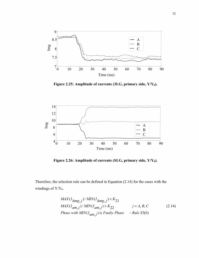
52
Figure 2.25: Amplitude of currents (3LG, primary side, Y/Y0).
Figure 2.26: Amplitude of currents (SLG, primary side, Y/Y0).
Therefore, the selection rule can be defined in Equation (2.14) for the cases with the
windings of Y/Y0.
( ) / ( ), , 21( ) / ( ) , ,, , 22
( ) 3( ),
MAX I MIN I Kmg j mg jMAX I MIN I K j A B Cam j am jPhase with MIN I is Faulty Phase Rule S bam j
<Δ Δ> =
−
(2.14)
0 10 20 30 40 50 60 70 80 907
7.5
8
8.5
9
Im
g
Time (ms)
A B C
0 10 20 30 40 50 60 70 80 904
6
8
10
12
14
Time (ms)
Im
g
A B C
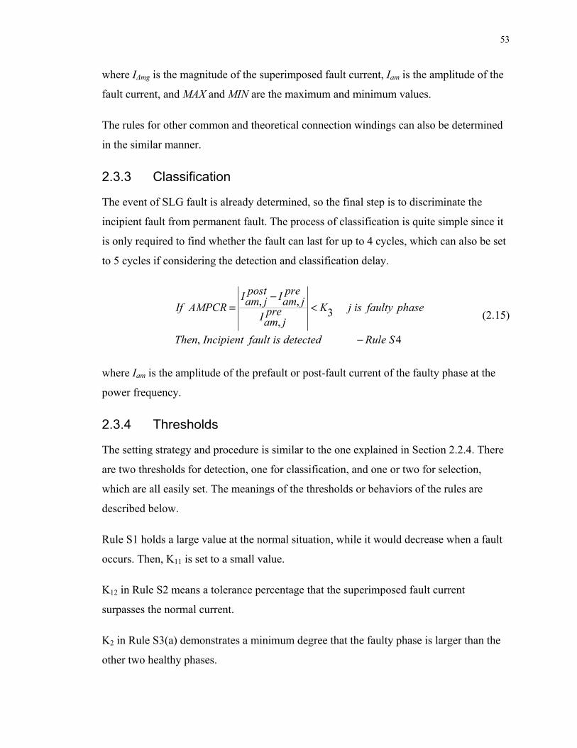
53
where IΔmg is the magnitude of the superimposed fault current, Iam is the amplitude of the
fault current, and MAX and MIN are the maximum and minimum values.
The rules for other common and theoretical connection windings can also be determined
in the similar manner.
2.3.3 Classification
The event of SLG fault is already determined, so the final step is to discriminate the
incipient fault from permanent fault. The process of classification is quite simple since it
is only required to find whether the fault can last for up to 4 cycles, which can also be set
to 5 cycles if considering the detection and classification delay.
, ,3
,
, 4
post preI Iam j am jIf AMPCR K j is faulty phasepreIam j
Then Incipient fault is detected Rule S
−= <
−
(2.15)
where Iam is the amplitude of the prefault or post-fault current of the faulty phase at the
power frequency.
2.3.4 Thresholds
The setting strategy and procedure is similar to the one explained in Section 2.2.4. There
are two thresholds for detection, one for classification, and one or two for selection,
which are all easily set. The meanings of the thresholds or behaviors of the rules are
described below.
Rule S1 holds a large value at the normal situation, while it would decrease when a fault
occurs. Then, K11 is set to a small value.
K12 in Rule S2 means a tolerance percentage that the superimposed fault current
surpasses the normal current.
K2 in Rule S3(a) demonstrates a minimum degree that the faulty phase is larger than the
other two healthy phases.
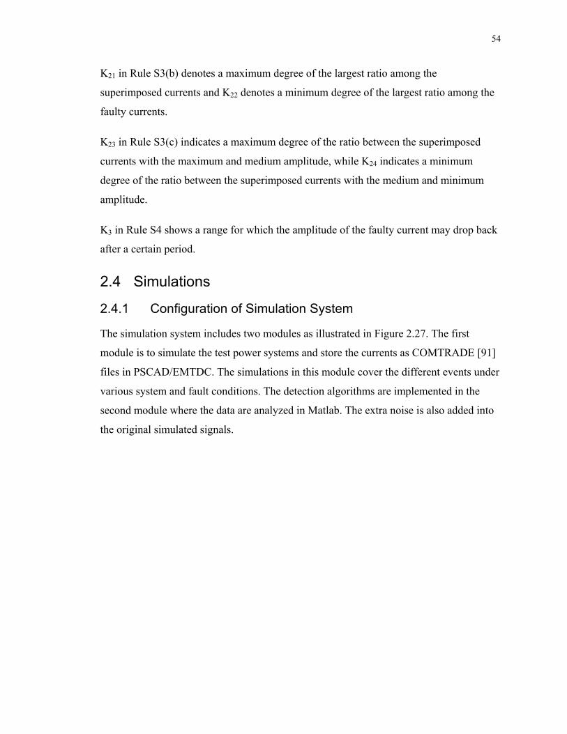
54
K21 in Rule S3(b) denotes a maximum degree of the largest ratio among the
superimposed currents and K22 denotes a minimum degree of the largest ratio among the
faulty currents.
K23 in Rule S3(c) indicates a maximum degree of the ratio between the superimposed
currents with the maximum and medium amplitude, while K24 indicates a minimum
degree of the ratio between the superimposed currents with the medium and minimum
amplitude.
K3 in Rule S4 shows a range for which the amplitude of the faulty current may drop back
after a certain period.
2.4 Simulations
2.4.1 Configuration of Simulation System
The simulation system includes two modules as illustrated in Figure 2.27. The first
module is to simulate the test power systems and store the currents as COMTRADE [91]
files in PSCAD/EMTDC. The simulations in this module cover the different events under
various system and fault conditions. The detection algorithms are implemented in the
second module where the data are analyzed in Matlab. The extra noise is also added into
the original simulated signals.
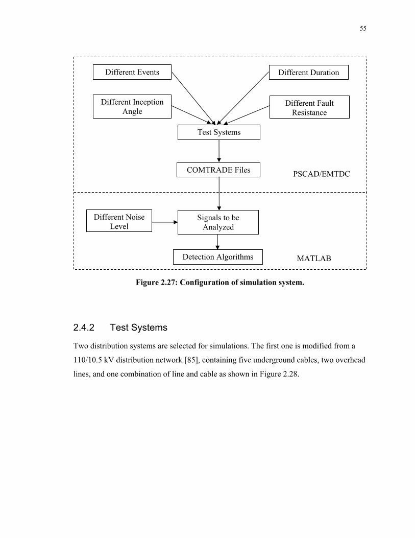
55
Figure 2.27: Configuration of simulation system.
2.4.2 Test Systems
Two distribution systems are selected for simulations. The first one is modified from a
110/10.5 kV distribution network [85], containing five underground cables, two overhead
lines, and one combination of line and cable as shown in Figure 2.28.
Different Events Different Duration
Different Inception Angle
Different Fault Resistance
Test Systems
COMTRADE Files PSCAD/EMTDC
Different Noise Level
Signals to be Analyzed
Detection Algorithms MATLAB
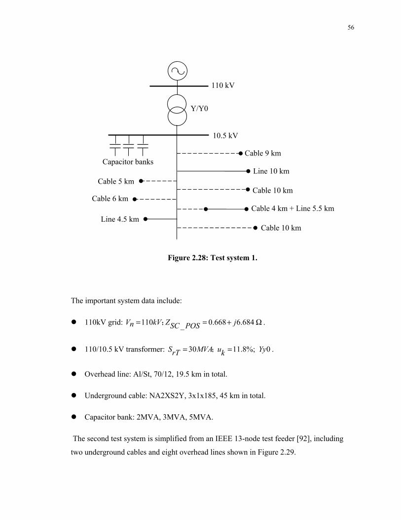
56
Figure 2.28: Test system 1.
The important system data include:
110kV grid: 110 0.668 6.684_V kV Z jn SC POS= = + Ω; .
110/10.5 kV transformer: 30 11.8%; 0S MVA u YyrT k= =; .
Overhead line: Al/St, 70/12, 19.5 km in total.
Underground cable: NA2XS2Y, 3x1x185, 45 km in total.
Capacitor bank: 2MVA, 3MVA, 5MVA.
The second test system is simplified from an IEEE 13-node test feeder [92], including
two underground cables and eight overhead lines shown in Figure 2.29.
Y/Y0
Cable 9 km
Line 10 km
Cable 10 km
110 kV
10.5 kV
Cable 4 km + Line 5.5 km
Cable 10 km
Cable 5 km
Cable 6 km
Line 4.5 km
Capacitor banks
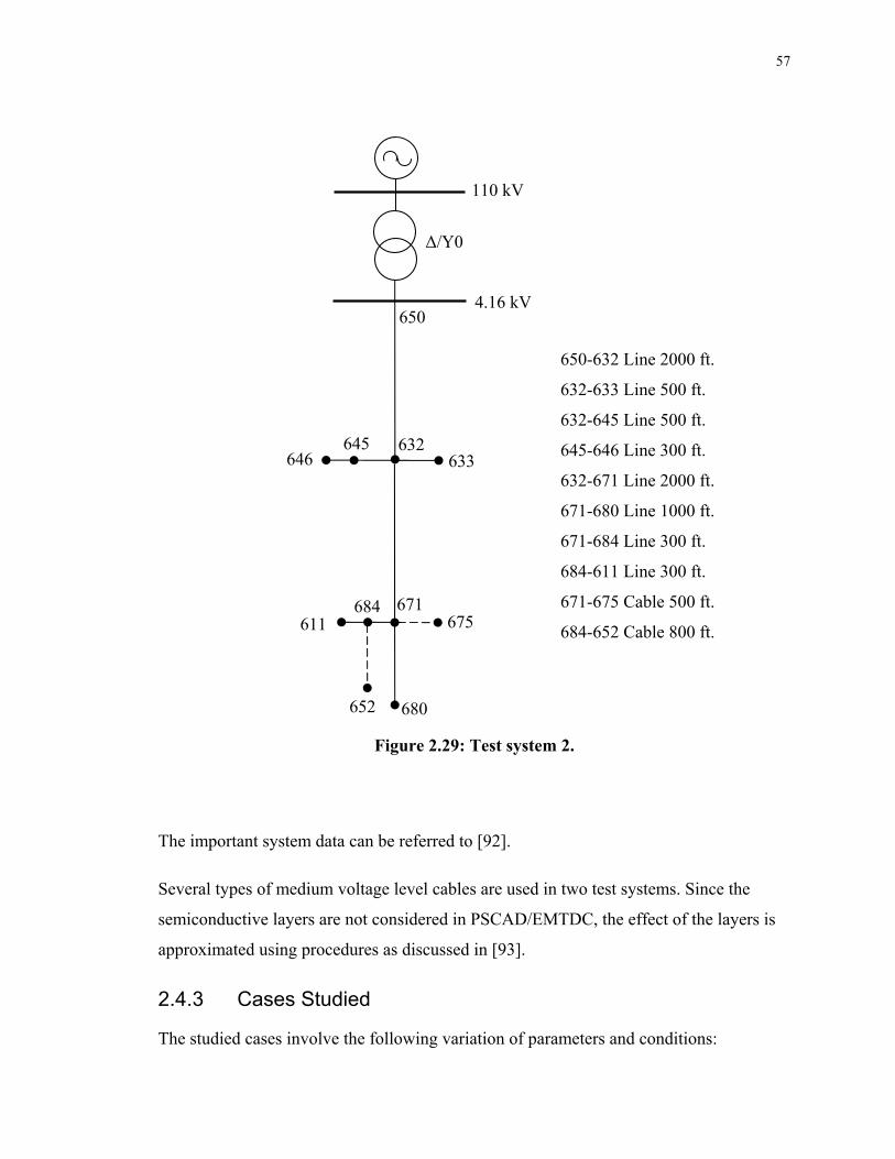
57
Figure 2.29: Test system 2.
The important system data can be referred to [92].
Several types of medium voltage level cables are used in two test systems. Since the
semiconductive layers are not considered in PSCAD/EMTDC, the effect of the layers is
approximated using procedures as discussed in [93].
2.4.3 Cases Studied
The studied cases involve the following variation of parameters and conditions:
Δ/Y0
650
650-632 Line 2000 ft.
632-633 Line 500 ft.
632-645 Line 500 ft.
645-646 Line 300 ft.
632-671 Line 2000 ft.
671-680 Line 1000 ft.
671-684 Line 300 ft.
684-611 Line 300 ft.
671-675 Cable 500 ft.
684-652 Cable 800 ft.
110 kV
4.16 kV
632 633
645 646
671
680
675 684
611
652

58
Noise levels, white noise are mixed into simulated data to make SNR (Signal-to-
Noise Ratio) range from 8.8 to 44 dB;
Fault distances, close-in terminal to far-end terminal in different feeders;
Fault types, balanced and unbalanced, grounded and ungrounded;
Fault resistances, zero to 50 ohm;
Fault inception angles, 0-270 degree;
CT locations, feeder, secondary and primary;
Transformer windings;
Capacitor and load switching;
Relay auto-reclosure;
Unbalanced/Balanced load;
Faults in underground cables and overhead lines.
2.4.4 Simulation Results
2.4.4.1 Wavelet-based Scheme
Simulated in the wavelet-based scheme, this group of simulations concerns the various
noise levels in the measured currents, different fault conditions, and other transient
events. The total amount of 404 events is simulated and each event is simulated more
than 300 times in a wide range of noise levels. The detection and classification results are
given in Table 2.1.
It is evident that there is no false detection. Also it can be found that not all of the events
can be detected correctly, nevertheless, it does not mean the proposed algorithm cannot
obtain the desired performance. When SNR=44dB, 20 undetected sub-cycle faults and 12
undetected multi-cycle faults have the relatively high fault resistance, so the currents
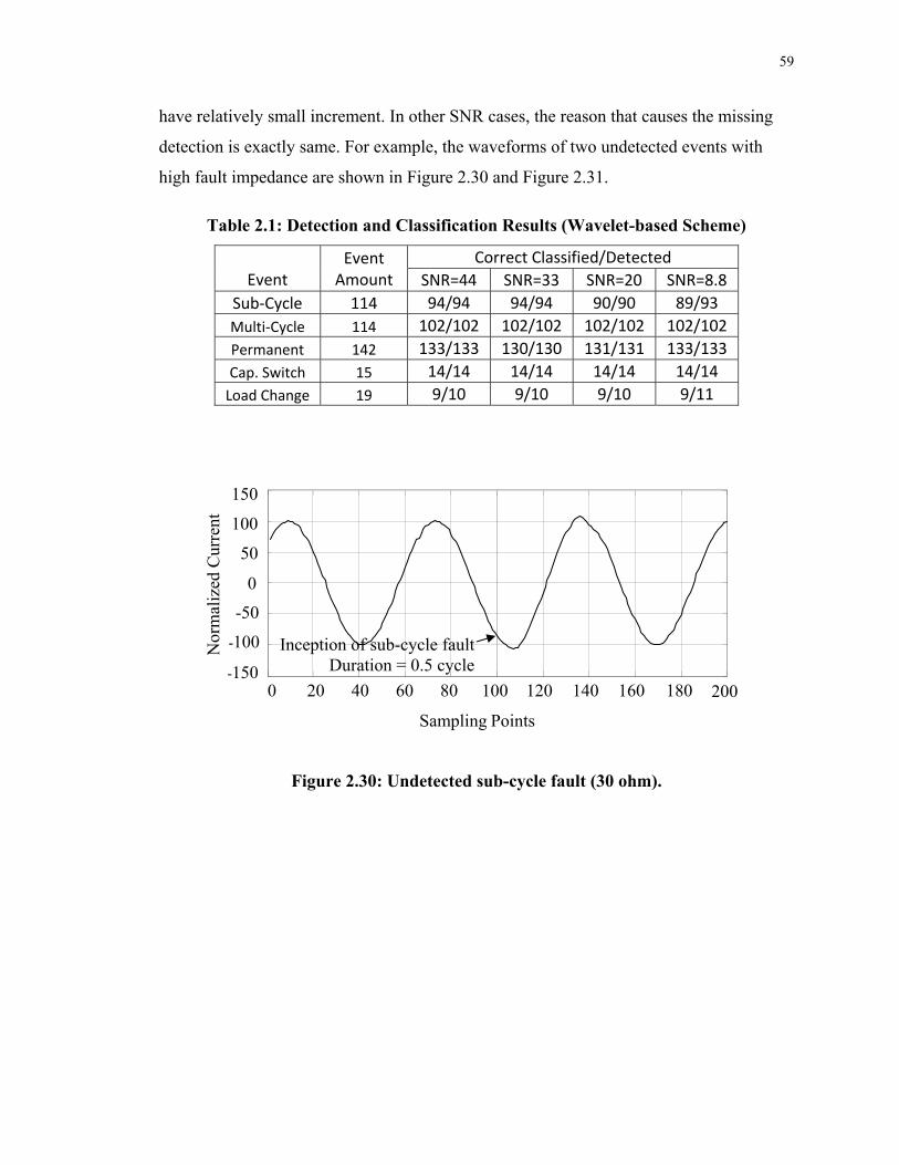
59
have relatively small increment. In other SNR cases, the reason that causes the missing
detection is exactly same. For example, the waveforms of two undetected events with
high fault impedance are shown in Figure 2.30 and Figure 2.31.
Table 2.1: Detection and Classification Results (Wavelet-based Scheme)
Correct Classified/Detected Event
Event Amount SNR=44 SNR=33 SNR=20 SNR=8.8
Sub-Cycle 114 94/94 94/94 90/90 89/93 Multi-Cycle 114 102/102 102/102 102/102 102/102 Permanent 142 133/133 130/130 131/131 133/133 Cap. Switch 15 14/14 14/14 14/14 14/14
Load Change 19 9/10 9/10 9/10 9/11
Figure 2.30: Undetected sub-cycle fault (30 ohm).
0 20 40 60 80 100 120 140 160 180 200
Sampling Points
Inception of sub-cycle faultDuration = 0.5 cycle
-150
-100
-50
50
100
150
Nor
mal
ized
Cur
rent
0
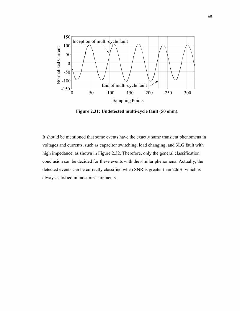
60
Figure 2.31: Undetected multi-cycle fault (50 ohm).
It should be mentioned that some events have the exactly same transient phenomena in
voltages and currents, such as capacitor switching, load changing, and 3LG fault with
high impedance, as shown in Figure 2.32. Therefore, only the general classification
conclusion can be decided for these events with the similar phenomena. Actually, the
detected events can be correctly classified when SNR is greater than 20dB, which is
always satisfied in most measurements.
0 50 100 150 200 250 300 -150
-100
-50
0
50
100
150 Inception of multi-cycle fault
End of multi-cycle fault
Sampling Points
Nor
mal
ized
Cur
rent
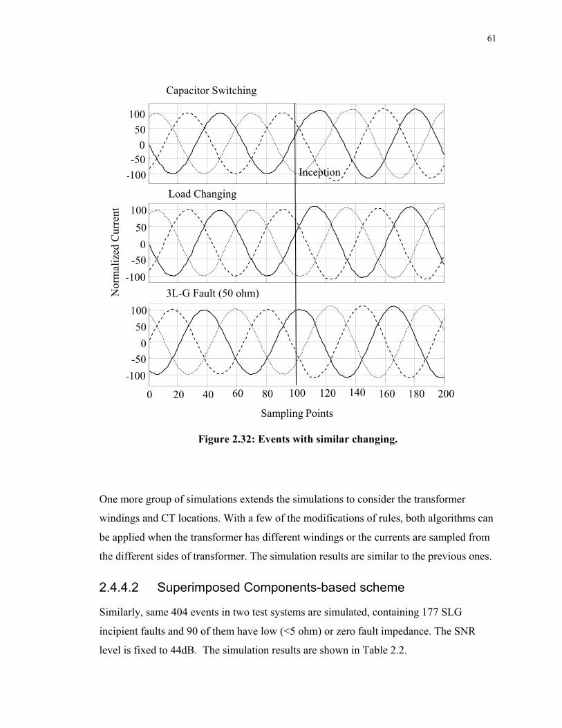
61
Figure 2.32: Events with similar changing.
One more group of simulations extends the simulations to consider the transformer
windings and CT locations. With a few of the modifications of rules, both algorithms can
be applied when the transformer has different windings or the currents are sampled from
the different sides of transformer. The simulation results are similar to the previous ones.
2.4.4.2 Superimposed Components-based scheme
Similarly, same 404 events in two test systems are simulated, containing 177 SLG
incipient faults and 90 of them have low (<5 ohm) or zero fault impedance. The SNR
level is fixed to 44dB. The simulation results are shown in Table 2.2.
-100
-50 0
50
100
-100
-50
0
50
100
0 20 40 60 80 100 120 140 160 180 200
-100
-50
0
50
100
Inception
Capacitor Switching
Load Changing
3L-G Fault (50 ohm)
Sampling Points
Nor
mal
ized
Cur
rent
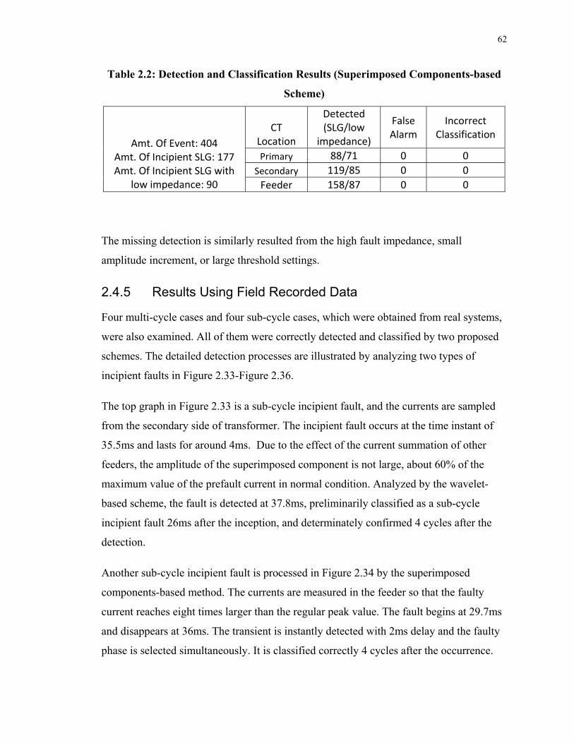
62
Table 2.2: Detection and Classification Results (Superimposed Components-based
Scheme)
CT Location
Detected (SLG/low
impedance)
False Alarm
Incorrect Classification
Primary 88/71 0 0 Secondary 119/85 0 0
Amt. Of Event: 404 Amt. Of Incipient SLG: 177 Amt. Of Incipient SLG with
low impedance: 90 Feeder 158/87 0 0
The missing detection is similarly resulted from the high fault impedance, small
amplitude increment, or large threshold settings.
2.4.5 Results Using Field Recorded Data
Four multi-cycle cases and four sub-cycle cases, which were obtained from real systems,
were also examined. All of them were correctly detected and classified by two proposed
schemes. The detailed detection processes are illustrated by analyzing two types of
incipient faults in Figure 2.33-Figure 2.36.
The top graph in Figure 2.33 is a sub-cycle incipient fault, and the currents are sampled
from the secondary side of transformer. The incipient fault occurs at the time instant of
35.5ms and lasts for around 4ms. Due to the effect of the current summation of other
feeders, the amplitude of the superimposed component is not large, about 60% of the
maximum value of the prefault current in normal condition. Analyzed by the wavelet-
based scheme, the fault is detected at 37.8ms, preliminarily classified as a sub-cycle
incipient fault 26ms after the inception, and determinately confirmed 4 cycles after the
detection.
Another sub-cycle incipient fault is processed in Figure 2.34 by the superimposed
components-based method. The currents are measured in the feeder so that the faulty
current reaches eight times larger than the regular peak value. The fault begins at 29.7ms
and disappears at 36ms. The transient is instantly detected with 2ms delay and the faulty
phase is selected simultaneously. It is classified correctly 4 cycles after the occurrence.
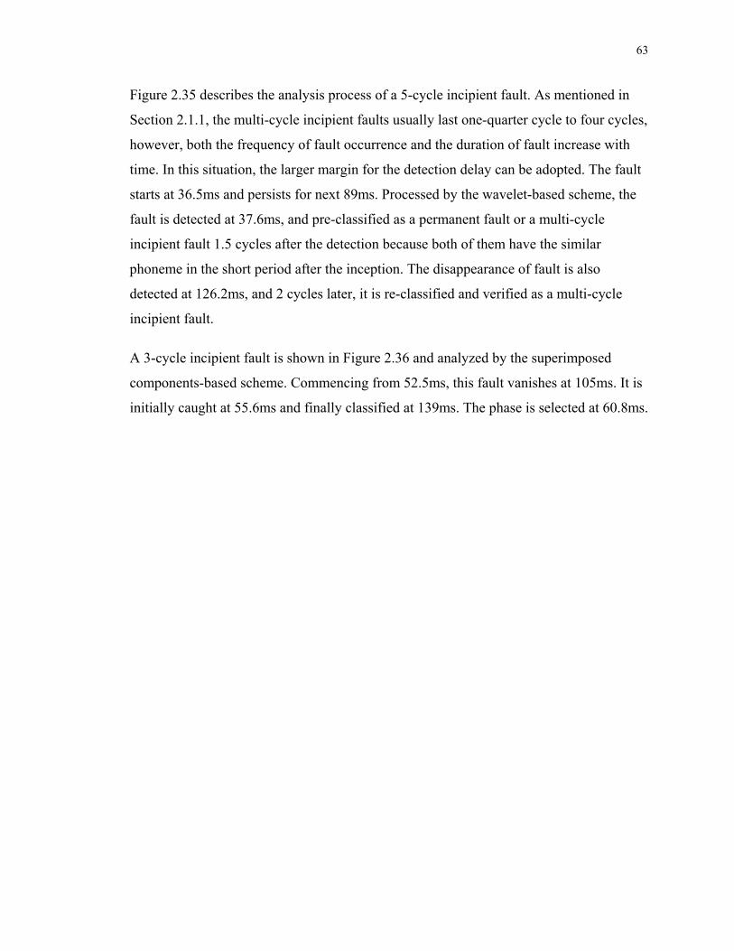
63
Figure 2.35 describes the analysis process of a 5-cycle incipient fault. As mentioned in
Section 2.1.1, the multi-cycle incipient faults usually last one-quarter cycle to four cycles,
however, both the frequency of fault occurrence and the duration of fault increase with
time. In this situation, the larger margin for the detection delay can be adopted. The fault
starts at 36.5ms and persists for next 89ms. Processed by the wavelet-based scheme, the
fault is detected at 37.6ms, and pre-classified as a permanent fault or a multi-cycle
incipient fault 1.5 cycles after the detection because both of them have the similar
phoneme in the short period after the inception. The disappearance of fault is also
detected at 126.2ms, and 2 cycles later, it is re-classified and verified as a multi-cycle
incipient fault.
A 3-cycle incipient fault is shown in Figure 2.36 and analyzed by the superimposed
components-based scheme. Commencing from 52.5ms, this fault vanishes at 105ms. It is
initially caught at 55.6ms and finally classified at 139ms. The phase is selected at 60.8ms.
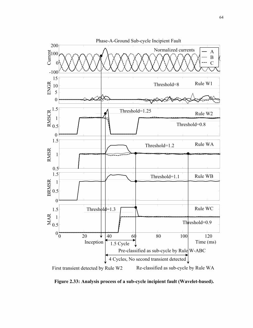
64
Figure 2.33: Analysis process of a sub-cycle incipient fault (Wavelet-based).
-100
0
100
200 Normalized currents
Phase-A-Ground Sub-cycle Incipient Fault
0
5 10
15 Threshold=8 Rule W1
0
0.5
1
1.5 Threshold=1.25
Threshold=0.8
Rule W2
0.5
1
1.5 Threshold=1.2 Rule WA
0
0.5
1
1.5 Threshold=1.1 Rule WB
0 20 40 60 80 100 1200
0.5
1
1.5 Threshold=1.3
Threshold=0.9
Rule WC
A B C
Inception 1.5 Cycle
Pre-classified as sub-cycle by Rule W-ABC
4 Cycles, No second transient detected
First transient detected by Rule W2 Re-classified as sub-cycle by Rule WA
Time (ms)
MA
R
B
RM
SR
RM
SR
R
MS
CR
EN
GR
Cur
rent
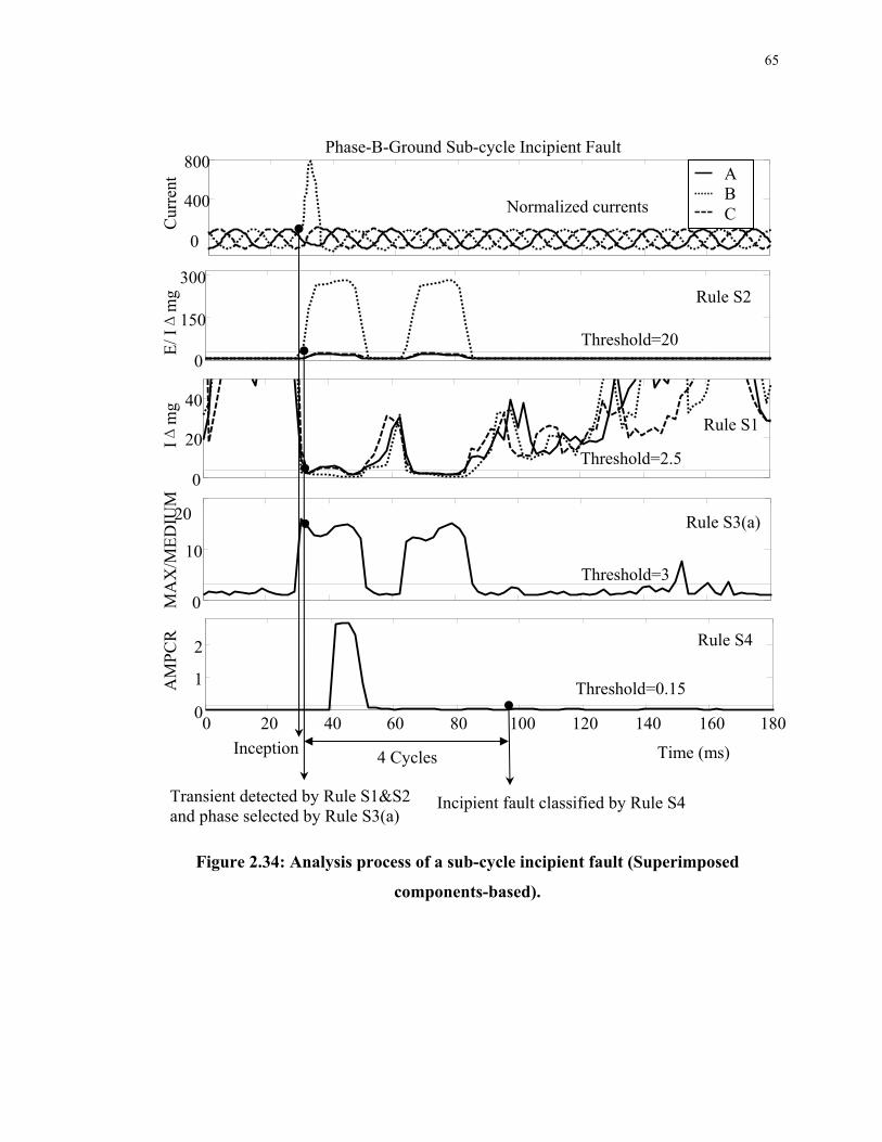
65
Figure 2.34: Analysis process of a sub-cycle incipient fault (Superimposed
components-based).
0
400
800
Normalized currents
Phase-B-Ground Sub-cycle Incipient Fault
0
150
300
Threshold=20
Rule S2
0
20
40
Threshold=2.5
Rule S1
0
10
20
Threshold=3
Rule S3(a)
0 20 40 60 80 100 120 140 160 1800
1
2
Threshold=0.15
Rule S4
AM
PC
R
MA
X/M
ED
IUM
IΔ
mg
E
/ IΔ
mg
Cur
rent
A B C
Inception
Transient detected by Rule S1&S2 and phase selected by Rule S3(a)
4 Cycles
Incipient fault classified by Rule S4
Time (ms)
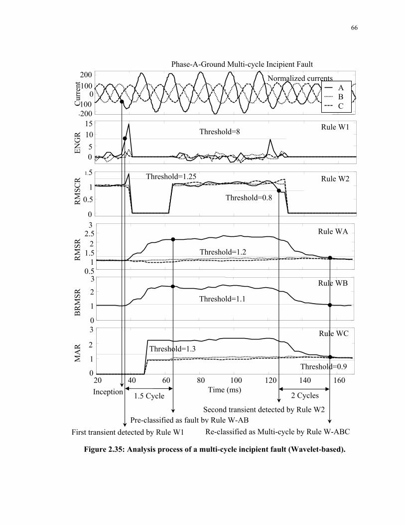
66
Figure 2.35: Analysis process of a multi-cycle incipient fault (Wavelet-based).
-200 -100
0 100
200 Normalized currents
Phase-A-Ground Multi-cycle Incipient Fault
0 5
10 15
Threshold=8Rule W1
0
0.5
1
1.5 Threshold=1.25
Threshold=0.8
Rule W2
0.5 1
1.5 2
2.5 3
Threshold=1.2
Rule WA
0
1
2
3
Threshold=1.1
Rule WB
20 40 60 80 100 120 140 1600
1
2
3
Threshold=1.3
Threshold=0.9
Rule WC
A B C
1.5 Cycle 2 Cycles Inception
Second transient detected by Rule W2 Pre-classified as fault by Rule W-AB
First transient detected by Rule W1 Re-classified as Multi-cycle by Rule W-ABC
Time (ms)
MA
R
B
RM
SR
RM
SR
R
MS
CR
EN
GR
Cur
rent
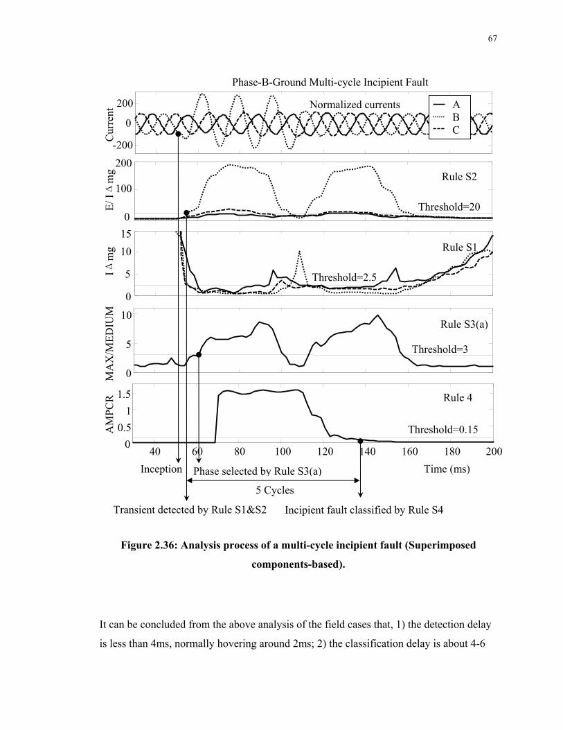
67
Figure 2.36: Analysis process of a multi-cycle incipient fault (Superimposed
components-based).
It can be concluded from the above analysis of the field cases that, 1) the detection delay
is less than 4ms, normally hovering around 2ms; 2) the classification delay is about 4-6
-200
0
200 Normalized currents
Phase-B-Ground Multi-cycle Incipient Fault
0
100
200
Threshold=20
Rule S2
0
5
10
15
Threshold=2.5
Rule S1
0
5
10
Threshold=3
Rule S3(a)
40 60 80 100 120 140 160 180 2000
0.5
1
1.5
Threshold=0.15
Rule 4
A B C
AM
PC
R
MA
X/M
ED
IUM
IΔ
mg
E/ IΔ
mg
C
urre
nt
Inception
Transient detected by Rule S1&S2
Phase selected by Rule S3(a)
5 Cycles
Incipient fault classified by Rule S4
Time (ms)
68
cycles after the detection; 3) the fault can be detected even if its duration is as short as
4ms; 4) the fault can be detected even if its superimposed amplitude is as less as 60% of
the regular peak value. In addition, these conclusions are verified by the simulation cases
in PSCAD/EMTDC.
69
Chapter 3
3 Fault Location Algorithms for Medium Voltage Cables
The fault location in underground cables is characterized as the technical difficulties due
to the complexities in cables. Based on the direct circuit analysis, a set of location
algorithms are proposed to locate the single phase related faults in the typical single-
conductor cross-linked polyethylene (XLPE) cables rated at the medium voltage levels. A
number of complex equations are effectively solved to find the fault distance and fault
resistance. The algorithms only utilize the fundamental phasors of three-phase voltages
and currents recorded at the substation. Particularly, the distinctive cable characteristics
are considered, such as the effects of shunt capacitance, effects of metallic sheaths and
common sheath bonding methods. The different fault scenarios are taken into account as
well.
The background knowledge is first introduced, including the structure of a typical XLPE
cable, the common sheath bonding methods, the complexities existing in fault location
calculations for cables and the different fault scenarios. Then a two-layer π model is
formulated to approximate the characteristics and behaviors of a typical MV XLPE cable.
The principle and procedure of the location algorithms are specially explicated for a cable
with sheaths grounded at the sending terminal. The differences and similarities of the
algorithms for other bonding methods are compared and summarized as well. The
estimation of load impedance is discussed for the constant impedance load model and
static response load model respectively. The algorithms are examined on three types of
MV cables with different fault types, fault resistances, fault distances and bonding
methods in the last section of this chapter. The simulation studies demonstrate that the
proposed algorithm can achieve the high accuracy under various system and fault
conditions.
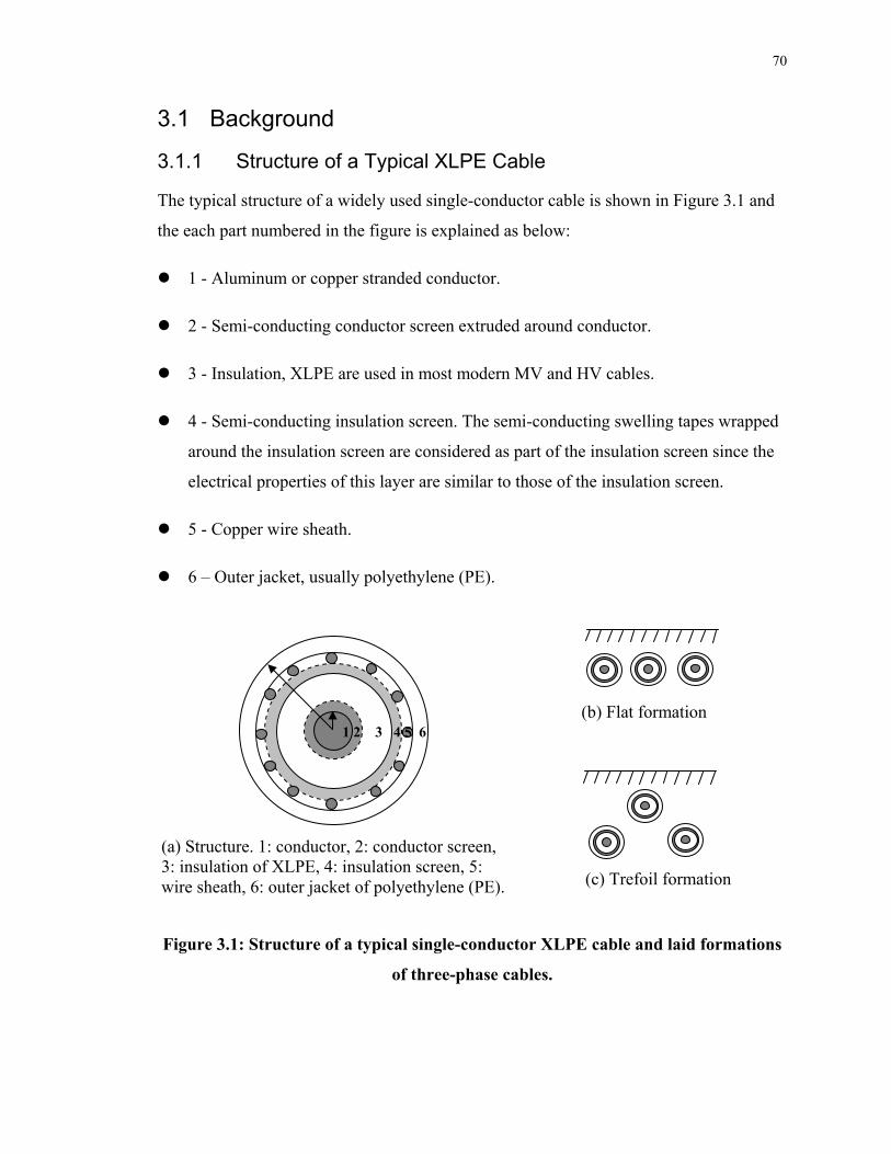
70
3.1 Background
3.1.1 Structure of a Typical XLPE Cable
The typical structure of a widely used single-conductor cable is shown in Figure 3.1 and
the each part numbered in the figure is explained as below:
1 - Aluminum or copper stranded conductor.
2 - Semi-conducting conductor screen extruded around conductor.
3 - Insulation, XLPE are used in most modern MV and HV cables.
4 - Semi-conducting insulation screen. The semi-conducting swelling tapes wrapped
around the insulation screen are considered as part of the insulation screen since the
electrical properties of this layer are similar to those of the insulation screen.
5 - Copper wire sheath.
6 – Outer jacket, usually polyethylene (PE).
Figure 3.1: Structure of a typical single-conductor XLPE cable and laid formations
of three-phase cables.
1 2 3 4 5 6
(a) Structure. 1: conductor, 2: conductor screen, 3: insulation of XLPE, 4: insulation screen, 5: wire sheath, 6: outer jacket of polyethylene (PE).
(b) Flat formation
(c) Trefoil formation
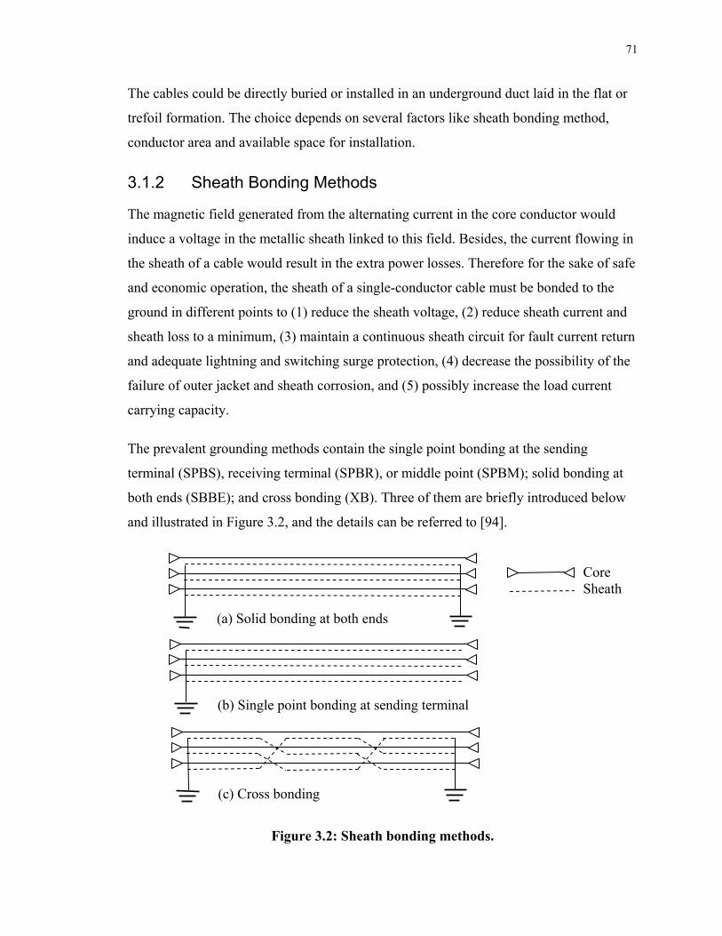
71
The cables could be directly buried or installed in an underground duct laid in the flat or
trefoil formation. The choice depends on several factors like sheath bonding method,
conductor area and available space for installation.
3.1.2 Sheath Bonding Methods
The magnetic field generated from the alternating current in the core conductor would
induce a voltage in the metallic sheath linked to this field. Besides, the current flowing in
the sheath of a cable would result in the extra power losses. Therefore for the sake of safe
and economic operation, the sheath of a single-conductor cable must be bonded to the
ground in different points to (1) reduce the sheath voltage, (2) reduce sheath current and
sheath loss to a minimum, (3) maintain a continuous sheath circuit for fault current return
and adequate lightning and switching surge protection, (4) decrease the possibility of the
failure of outer jacket and sheath corrosion, and (5) possibly increase the load current
carrying capacity.
The prevalent grounding methods contain the single point bonding at the sending
terminal (SPBS), receiving terminal (SPBR), or middle point (SPBM); solid bonding at
both ends (SBBE); and cross bonding (XB). Three of them are briefly introduced below
and illustrated in Figure 3.2, and the details can be referred to [94].
Figure 3.2: Sheath bonding methods.
(a) Solid bonding at both ends
(b) Single point bonding at sending terminal
(c) Cross bonding
Core Sheath

72
The solid bonding method grounds sheaths at both ends, which can reduce the induced
voltage. The disadvantages of this bonding method include that it provides the loop path
for circulating currents at normal operation conditions, causes power losses in sheaths,
and further reduces the cable ampacity. The single-point bonding method grounds sheaths
at one point along the cable circuit, typically at one of the two terminals or at the middle
point of a cable. Although there are no significant circulating currents flowing in sheaths,
a voltage will be induced between the core conductor and sheath and between the sheath
and earth. Therefore, the surge voltage limiters must be used to protect the floating end of
sheaths from overvoltage danger. The cross bonding method grounds sheaths at both ends
and sheaths are cross-connected at the joints by which the cable is sectionalized into three
sections of equal length. The circulating currents and power losses are significantly
reduced and the induced voltages are partially neutralized as well. The maximum induced
voltage appears at the joint boxes.
3.1.3 Complexities in Fault Location for Cables
The location principles for underground cables are comparatively different from the ones
for overhead transmission lines or distribution lines due to the following electrical
characteristics of cables [95]-[99].
The impedance per unit length of cables is less than that of lines.
The series inductance of cables is typically 30~50% lower than that of lines.
The shunt capacitance of cables is 30~40 times higher than that of lines.
The zero-sequence impedance of cables is not constant and depends on many factors,
such as bonding method, fault current, presence of parallel circuit and resistivity of
ground.
The zero-sequence impedance angle of cables is less than that of lines.
The X/R ratio of cables is much lower than that of lines.
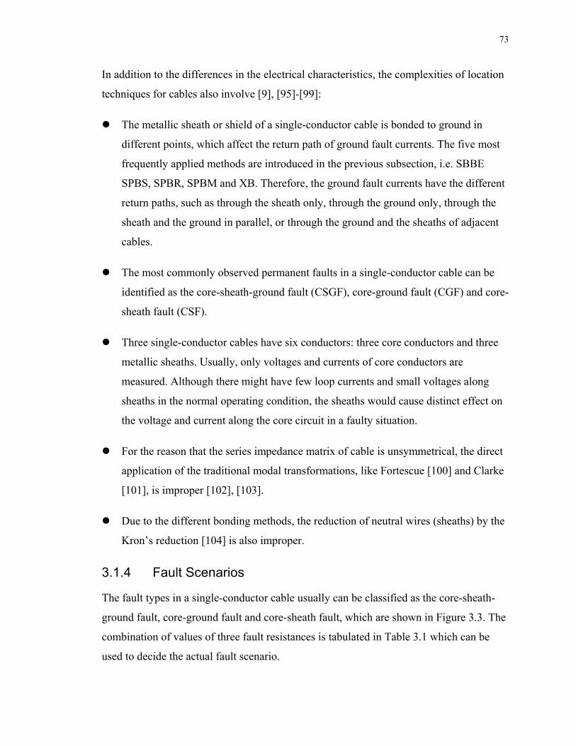
73
In addition to the differences in the electrical characteristics, the complexities of location
techniques for cables also involve [9], [95]-[99]:
The metallic sheath or shield of a single-conductor cable is bonded to ground in
different points, which affect the return path of ground fault currents. The five most
frequently applied methods are introduced in the previous subsection, i.e. SBBE
SPBS, SPBR, SPBM and XB. Therefore, the ground fault currents have the different
return paths, such as through the sheath only, through the ground only, through the
sheath and the ground in parallel, or through the ground and the sheaths of adjacent
cables.
The most commonly observed permanent faults in a single-conductor cable can be
identified as the core-sheath-ground fault (CSGF), core-ground fault (CGF) and core-
sheath fault (CSF).
Three single-conductor cables have six conductors: three core conductors and three
metallic sheaths. Usually, only voltages and currents of core conductors are
measured. Although there might have few loop currents and small voltages along
sheaths in the normal operating condition, the sheaths would cause distinct effect on
the voltage and current along the core circuit in a faulty situation.
For the reason that the series impedance matrix of cable is unsymmetrical, the direct
application of the traditional modal transformations, like Fortescue [100] and Clarke
[101], is improper [102], [103].
Due to the different bonding methods, the reduction of neutral wires (sheaths) by the
Kron’s reduction [104] is also improper.
3.1.4 Fault Scenarios
The fault types in a single-conductor cable usually can be classified as the core-sheath-
ground fault, core-ground fault and core-sheath fault, which are shown in Figure 3.3. The
combination of values of three fault resistances is tabulated in Table 3.1 which can be
used to decide the actual fault scenario.
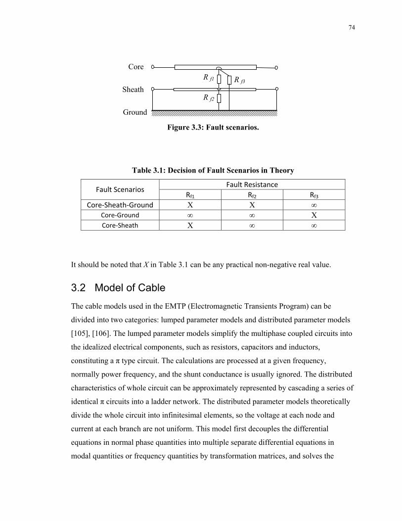
74
Figure 3.3: Fault scenarios.
Table 3.1: Decision of Fault Scenarios in Theory
Fault Resistance Fault Scenarios Rf1 Rf2 Rf3
Core-Sheath-Ground X X ∞ Core-Ground ∞ ∞ X Core-Sheath X ∞ ∞
It should be noted that X in Table 3.1 can be any practical non-negative real value.
3.2 Model of Cable
The cable models used in the EMTP (Electromagnetic Transients Program) can be
divided into two categories: lumped parameter models and distributed parameter models
[105], [106]. The lumped parameter models simplify the multiphase coupled circuits into
the idealized electrical components, such as resistors, capacitors and inductors,
constituting a π type circuit. The calculations are processed at a given frequency,
normally power frequency, and the shunt conductance is usually ignored. The distributed
characteristics of whole circuit can be approximately represented by cascading a series of
identical π circuits into a ladder network. The distributed parameter models theoretically
divide the whole circuit into infinitesimal elements, so the voltage at each node and
current at each branch are not uniform. This model first decouples the differential
equations in normal phase quantities into multiple separate differential equations in
modal quantities or frequency quantities by transformation matrices, and solves the
R f3R f1
R f2Sheath
Ground
Core
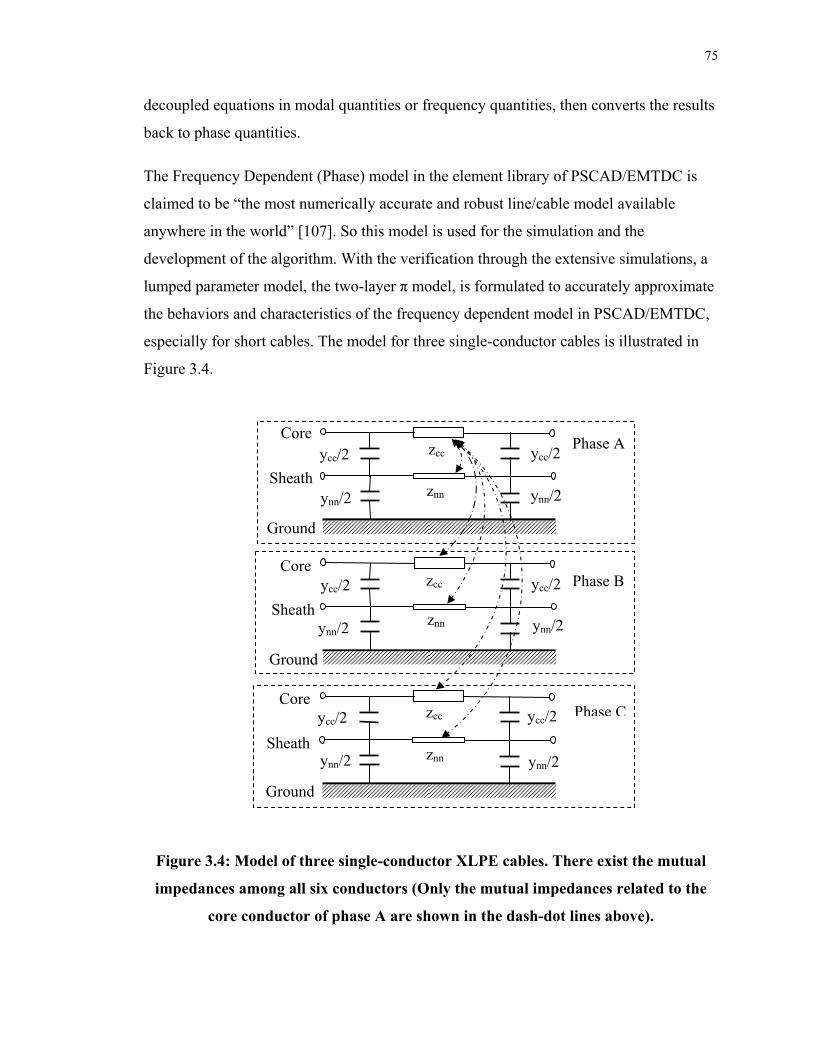
75
decoupled equations in modal quantities or frequency quantities, then converts the results
back to phase quantities.
The Frequency Dependent (Phase) model in the element library of PSCAD/EMTDC is
claimed to be “the most numerically accurate and robust line/cable model available
anywhere in the world” [107]. So this model is used for the simulation and the
development of the algorithm. With the verification through the extensive simulations, a
lumped parameter model, the two-layer π model, is formulated to accurately approximate
the behaviors and characteristics of the frequency dependent model in PSCAD/EMTDC,
especially for short cables. The model for three single-conductor cables is illustrated in
Figure 3.4.
Figure 3.4: Model of three single-conductor XLPE cables. There exist the mutual
impedances among all six conductors (Only the mutual impedances related to the
core conductor of phase A are shown in the dash-dot lines above).
Phase A
Phase C
Phase B
Core
znn
ycc/2 ycc/2
ynn/2 ynn/2 Sheath
Ground
Core
znn
ycc/2 ycc/2
ynn/2 ynn/2 Sheath
Ground
Core
znn
ycc/2 ycc/2
ynn/2 ynn/2 Sheath
Ground
zcc
zcc
zcc
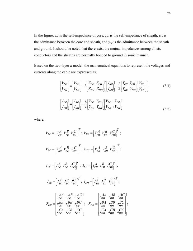
76
In the figure, zcc is the self-impedance of core, znn is the self-impedance of sheath, ycn is
the admittance between the core and sheath, and yng is the admittance between the sheath
and ground. It should be noted that there exist the mutual impedances among all six
conductors and the sheaths are normally bonded to ground in some manner.
Based on the two-layer π model, the mathematical equations to represent the voltages and
currents along the cable are expressed as,
2
V V Z Z I Y Y Vrc sc cc cn sc cc cn scLLV V Z Z I Y Y Vrn sn nc nn sn nc nn sn
= − − (3.1)
2
I I Y Y V Vrc sc cc cn sc rcLI I Y Y V Vrn sn nc nn sn rn
+= −
+ (3.2)
where,
; ;T TA B C A B CV V V V V V V Vrc rnrc rc rc rn rn rn
= =
; ;T TA B C A B CV V V V V V V Vsc snsc sc sc sn sn sn
= =
; ;T TA B C A B CI I I I I I I Irc rnrc rc rc rn rn rn
= =
; ;T TA B C A B CI I I I I I I Isc snsc sc sc sn sn sn
= =
; ;
AA AB AC AA AB ACz z z z z zcc cc cc nn nn nnBA BB BC BA BB BCZ z z z Z z z zcc nncc cc cc nn nn nnCA CB CC CA CB CCz z z z z zcc cc cc nn nn nn
= =
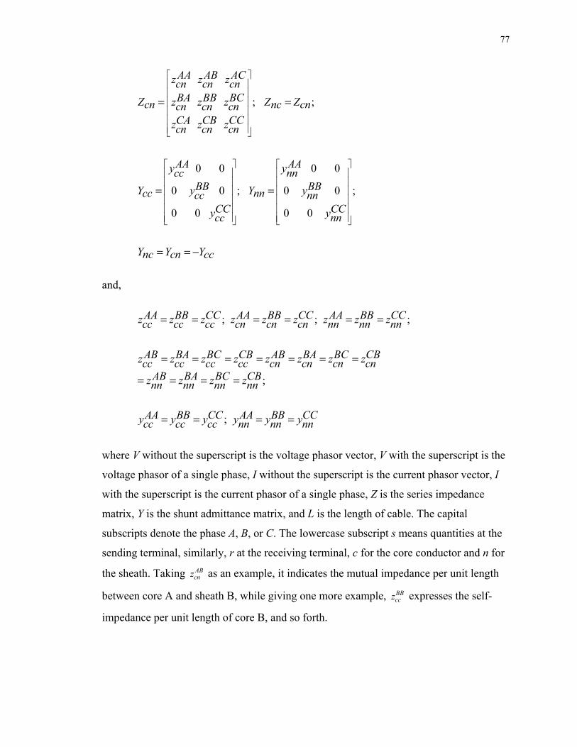
77
; ;
AA AB ACz z zcn cn cnBA BB BCZ z z z Z Zcn nc cncn cn cnCA CB CCz z zcn cn cn
= =
0 0 0 0
0 0 ; 0 0 ;
0 0 0 0
AA AAy ycc nnBB BBY y Y ycc nncc nn
CC CCy ycc nn
= =
Y Y Ync cn cc= = −
and,
; ; ;AA BB CC AA BB CC AA BB CCz z z z z z z z zcc cc cc cn cn cn nn nn nn= = = = = =
;
AB BA BC CB AB BA BC CBz z z z z z z zcc cc cc cc cn cn cn cnAB BA BC CBz z z znn nn nn nn
= = = = = = =
= = = =
;AA BB CC AA BB CCy y y y y ycc cc cc nn nn nn= = = =
where V without the superscript is the voltage phasor vector, V with the superscript is the
voltage phasor of a single phase, I without the superscript is the current phasor vector, I
with the superscript is the current phasor of a single phase, Z is the series impedance
matrix, Y is the shunt admittance matrix, and L is the length of cable. The capital
subscripts denote the phase A, B, or C. The lowercase subscript s means quantities at the
sending terminal, similarly, r at the receiving terminal, c for the core conductor and n for
the sheath. Taking ABcnz as an example, it indicates the mutual impedance per unit length
between core A and sheath B, while giving one more example, BBccz expresses the self-
impedance per unit length of core B, and so forth.
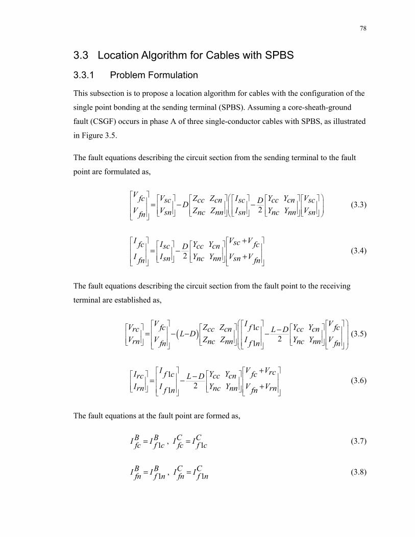
78
3.3 Location Algorithm for Cables with SPBS
3.3.1 Problem Formulation
This subsection is to propose a location algorithm for cables with the configuration of the
single point bonding at the sending terminal (SPBS). Assuming a core-sheath-ground
fault (CSGF) occurs in phase A of three single-conductor cables with SPBS, as illustrated
in Figure 3.5.
The fault equations describing the circuit section from the sending terminal to the fault
point are formulated as,
2
V V Z Z I Y Y Vfc sc cc cn sc cc cn scDDV V Z Z I Y Y Vsn nc nn sn nc nn snfn
= − − (3.3)
2
I V VscI Y Yfc fcsc cc cnDI I Y Y V Vsn nc nn snfn fn
+= −
+ (3.4)
The fault equations describing the circuit section from the fault point to the receiving
terminal are established as,
( ) 1
21
V I VV Z Z Y Yfc f c fcrc cc cn cc cnL DL DV V Z Z I Y Y Vrn nc nn nc nnfn f n fn
−= − − − (3.5)
1
21
I V VrcI Y Yf c fcrc cc cnL DI I Y Y V Vrn nc nn rnf n fn
+−= −
+ (3.6)
The fault equations at the fault point are formed as,
,1 1B B C CI I I Ifc f c fc f c= = (3.7)
,1 1B B C CI I I Ifn f n fn f n= = (3.8)
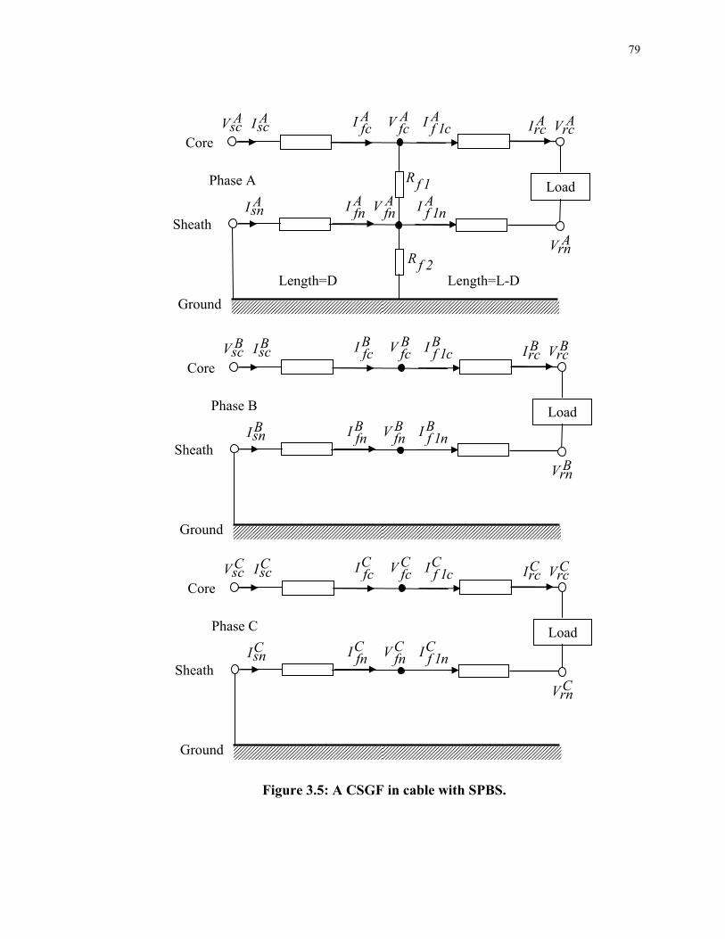
79
Figure 3.5: A CSGF in cable with SPBS.
Core
Sheath
Ground
Load Phase A
Length=D Length=L-D
A AI Vrc rc A A AI V Ifc fc f 1c
A AV Isc sc
AIsn A A AI V Ifn fn f 1n
AVrn
R f 1
R f 2
Core
Sheath
Ground
Load Phase B
B BI Vrc rc B B BI V Ifc fc f 1c
B BV Isc sc
BIsn B B BI V Ifn fn f 1n
BVrn
Core
Sheath
Ground
Load Phase C
C CI Vrc rc C C CI V Ifc fc f 1c
C CV Isc sc
CIsn C C CI V Ifn fn f 1n
CVrn
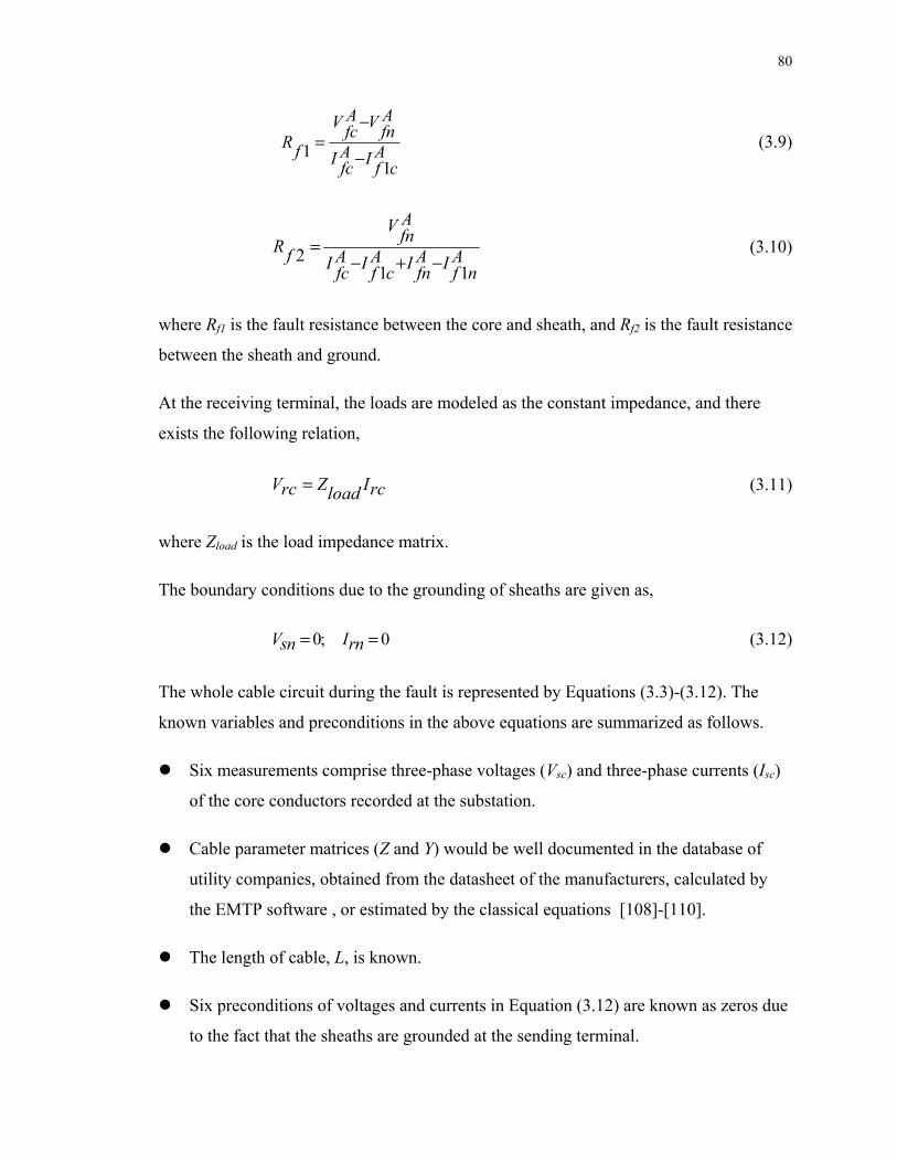
80
11
A AV Vfc fn
R f A AI Ifc f c
−=
− (3.9)
21 1
AVfn
R f A A A AI I I Ifc f c fn f n
=− + −
(3.10)
where Rf1 is the fault resistance between the core and sheath, and Rf2 is the fault resistance
between the sheath and ground.
At the receiving terminal, the loads are modeled as the constant impedance, and there
exists the following relation,
V Z Irc rcload= (3.11)
where Zload is the load impedance matrix.
The boundary conditions due to the grounding of sheaths are given as,
0; 0V Isn rn= = (3.12)
The whole cable circuit during the fault is represented by Equations (3.3)-(3.12). The
known variables and preconditions in the above equations are summarized as follows.
Six measurements comprise three-phase voltages (Vsc) and three-phase currents (Isc)
of the core conductors recorded at the substation.
Cable parameter matrices (Z and Y) would be well documented in the database of
utility companies, obtained from the datasheet of the manufacturers, calculated by
the EMTP software , or estimated by the classical equations [108]-[110].
The length of cable, L, is known.
Six preconditions of voltages and currents in Equation (3.12) are known as zeros due
to the fact that the sheaths are grounded at the sending terminal.
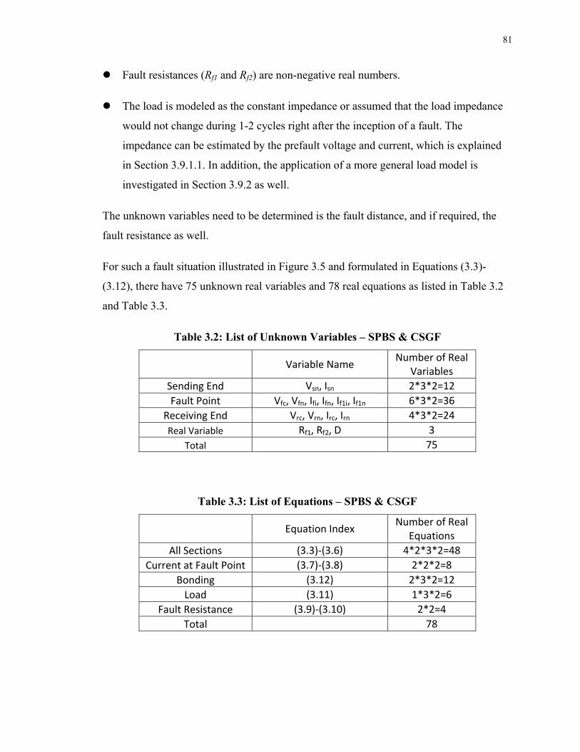
81
Fault resistances (Rf1 and Rf2) are non-negative real numbers.
The load is modeled as the constant impedance or assumed that the load impedance
would not change during 1-2 cycles right after the inception of a fault. The
impedance can be estimated by the prefault voltage and current, which is explained
in Section 3.9.1.1. In addition, the application of a more general load model is
investigated in Section 3.9.2 as well.
The unknown variables need to be determined is the fault distance, and if required, the
fault resistance as well.
For such a fault situation illustrated in Figure 3.5 and formulated in Equations (3.3)-
(3.12), there have 75 unknown real variables and 78 real equations as listed in Table 3.2
and Table 3.3.
Table 3.2: List of Unknown Variables – SPBS & CSGF
Variable Name Number of Real Variables
Sending End Vsn, Isn 2*3*2=12 Fault Point Vfc, Vfn, Ifi, Ifn, If1i, If1n 6*3*2=36
Receiving End Vrc, Vrn, Irc, Irn 4*3*2=24 Real Variable Rf1, Rf2, D 3
Total 75
Table 3.3: List of Equations – SPBS & CSGF
Equation Index Number of Real Equations
All Sections (3.3)-(3.6) 4*2*3*2=48 Current at Fault Point (3.7)-(3.8) 2*2*2=8
Bonding (3.12) 2*3*2=12 Load (3.11) 1*3*2=6
Fault Resistance (3.9)-(3.10) 2*2=4 Total 78

82
However, it is impractical and time-consuming to solve this set of equations by directly
using some mathematic solving tools, such as the solving functions in Matlab [111]. The
fast solving algorithm would be proposed in the next subsection.
3.3.2 Locating Core-Sheath-Ground Fault
The proposed algorithm in this subsection is to locate the single-phase core-sheath-
ground fault (CSGF) in three single-conductor cables, especially with sheaths only
grounded at the sending terminal.
It is doubtless that all variables in Equations (3.3)-(3.12) would be definitely solved
provided that the sheath currents (Isn) and fault distance (D) were known. There are six
real variables for Isn, which values are time-varying and the range is hardly predictable.
Nonetheless, there is only one real variable for D with a known range, i.e. from 0 to the
length of cable, L. Therefore, a conceptual framework is proposed that a set of fault
distances are first assumed, and then, the related sheath currents at the sending terminal
are estimated for each assumed distance, subsequently all unknown quantities are solved
by Equations (3.3)-(3.12), finally the exact fault point is accurately pinpointed.
3.3.2.1 Estimation of Sheath Currents of Healthy Cables
First, a fault distance (D) is assumed and three-phase sheath currents at the sending
terminal (Isn) are initially set to zeros or assigned to the values calculated from the
estimation for the previous assumed distance.
The voltages at the fault point are calculated by,
2 00
V Z Z I Y Y VVfc sc cc cn sccc cnsc DDI Y YV Z Z sn nc nnnc nnfn
= − − (3.13)
The currents at the immediate left side of the fault point are formulated as,
2
I V VscI Y Yfc fcsc cc cnDI I Y Y Vsn nc nnfn fn
+= − (3.14)
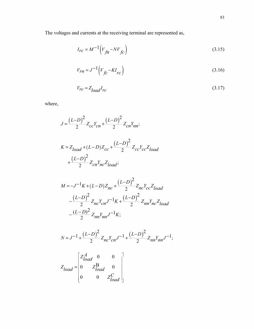
83
The voltages and currents at the receiving terminal are represented as,
( )1I M V NVrc fn fc−= − (3.15)
( )1V J V KIrn fc rc−= − (3.16)
V Z Irc rcload= (3.17)
where,
( ) ( )2 2;
2 2
L D L DJ Z Y Z Ycc cn cn nn
− −= +
( ) ( )
( )
2
22
;2
L DK Z L D Z Z Y Zcc cc ccload load
L DZ Y Zcn nc load
−= + − +
−+
( ) ( )
( ) ( )
21
22 2
12 2
2( ) 1 ;2
L DM J K L D Z Z Y Znc nc cc load
L D L DZ Y J K Z Y Znc cn nn nc load
L D Z Y J Knn nn
−−= − + − +
− −−− +
− −−
( ) ( )2 21 1 1;
2 2
L D L DN J Z Y J Z Y Jnc cn nn nn
− −− − −= + +
0 0
B0 0
0 0
AZload
Z Zload loadCZload
=
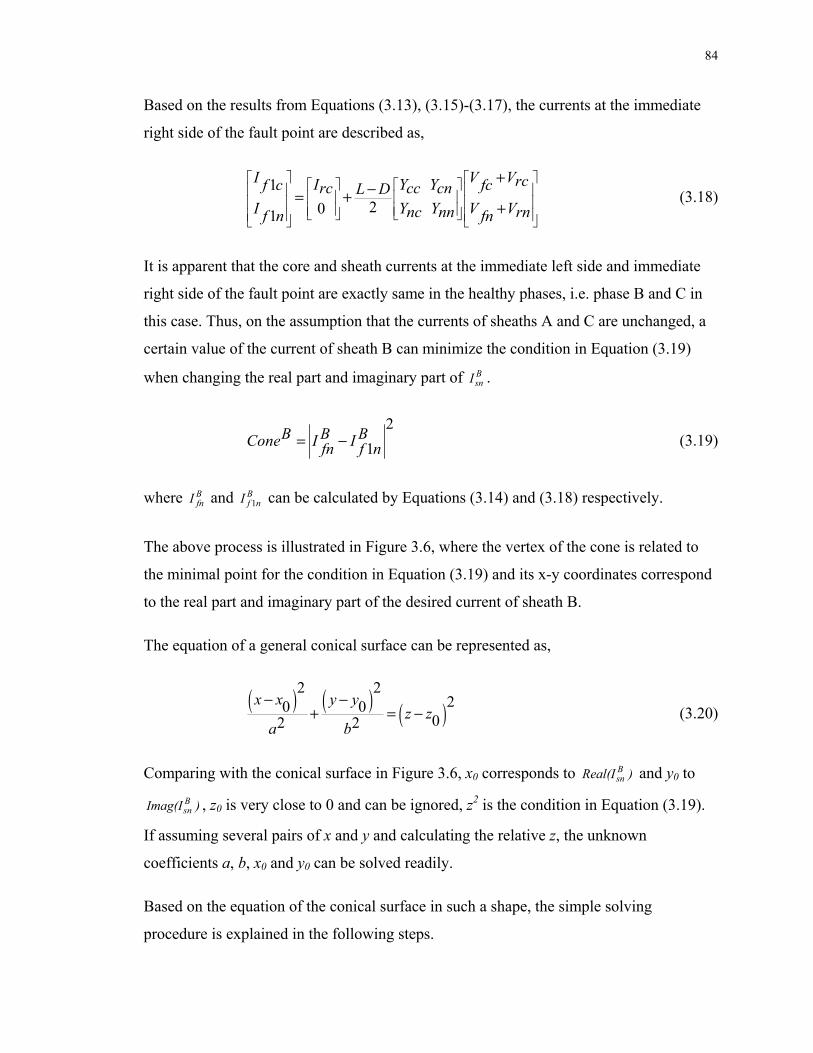
84
Based on the results from Equations (3.13), (3.15)-(3.17), the currents at the immediate
right side of the fault point are described as,
1
201
I V VrcY YIf c fccc cnrc L DI Y Y V Vnc nn rnf n fn
+−= +
+ (3.18)
It is apparent that the core and sheath currents at the immediate left side and immediate
right side of the fault point are exactly same in the healthy phases, i.e. phase B and C in
this case. Thus, on the assumption that the currents of sheaths A and C are unchanged, a
certain value of the current of sheath B can minimize the condition in Equation (3.19)
when changing the real part and imaginary part of BsnI .
2
1B B BCone I Ifn f n= − (3.19)
where BfnI and 1
Bf nI can be calculated by Equations (3.14) and (3.18) respectively.
The above process is illustrated in Figure 3.6, where the vertex of the cone is related to
the minimal point for the condition in Equation (3.19) and its x-y coordinates correspond
to the real part and imaginary part of the desired current of sheath B.
The equation of a general conical surface can be represented as,
( ) ( ) ( )2 2
20 002 2
x x y yz z
a b
− −+ = − (3.20)
Comparing with the conical surface in Figure 3.6, x0 corresponds to BsnReal(I ) and y0 to
BsnImag(I ) , z0 is very close to 0 and can be ignored, z2 is the condition in Equation (3.19).
If assuming several pairs of x and y and calculating the relative z, the unknown
coefficients a, b, x0 and y0 can be solved readily.
Based on the equation of the conical surface in such a shape, the simple solving
procedure is explained in the following steps.
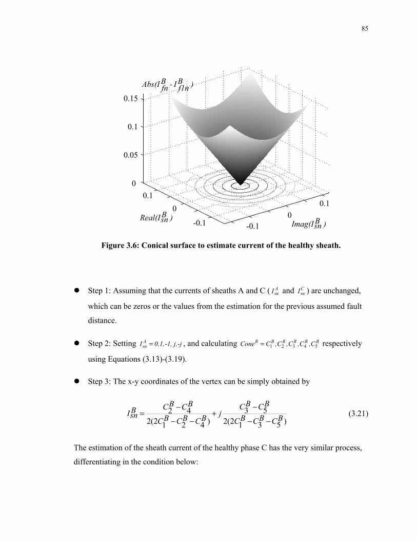
85
Figure 3.6: Conical surface to estimate current of the healthy sheath.
Step 1: Assuming that the currents of sheaths A and C ( AsnI and C
snI ) are unchanged,
which can be zeros or the values from the estimation for the previous assumed fault
distance.
Step 2: Setting AsnI 0,1,-1, j,-j= , and calculating 1 2 3 4 5
B B B B B BCone C ,C ,C ,C ,C= respectively
using Equations (3.13)-(3.19).
Step 3: The x-y coordinates of the vertex can be simply obtained by
532 42(2 ) 2(2 )51 2 4 1 3
B BB B C CC CBI jsn B B B B B BC C C C C C
−−= +
− − − − (3.21)
The estimation of the sheath current of the healthy phase C has the very similar process,
differentiating in the condition below:
BImag(I )sn BReal(I )sn
-0.10
0.1
-0.1
0
0.1
0.15 0.1
0.05
0
B BAbs(I - I )fn f1n
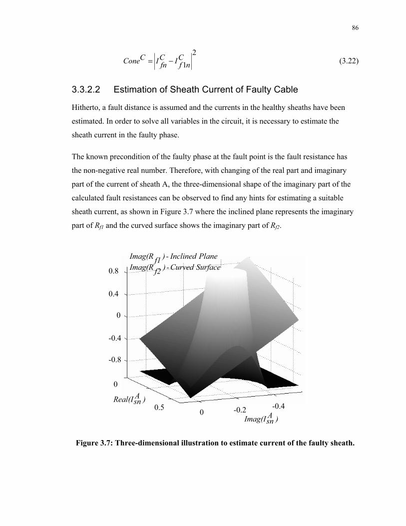
86
2
1C C CCone I Ifn f n= − (3.22)
3.3.2.2 Estimation of Sheath Current of Faulty Cable
Hitherto, a fault distance is assumed and the currents in the healthy sheaths have been
estimated. In order to solve all variables in the circuit, it is necessary to estimate the
sheath current in the faulty phase.
The known precondition of the faulty phase at the fault point is the fault resistance has
the non-negative real number. Therefore, with changing of the real part and imaginary
part of the current of sheath A, the three-dimensional shape of the imaginary part of the
calculated fault resistances can be observed to find any hints for estimating a suitable
sheath current, as shown in Figure 3.7 where the inclined plane represents the imaginary
part of Rf1 and the curved surface shows the imaginary part of Rf2.
Figure 3.7: Three-dimensional illustration to estimate current of the faulty sheath.
AImag(I )sn -0.20
-0.40.5
0
0.25
0.8
0.4
0
-0.4
-0.8
Imag(R )- Inclined Planef1Imag(R )- Curved Surfacef2
AReal(I )sn
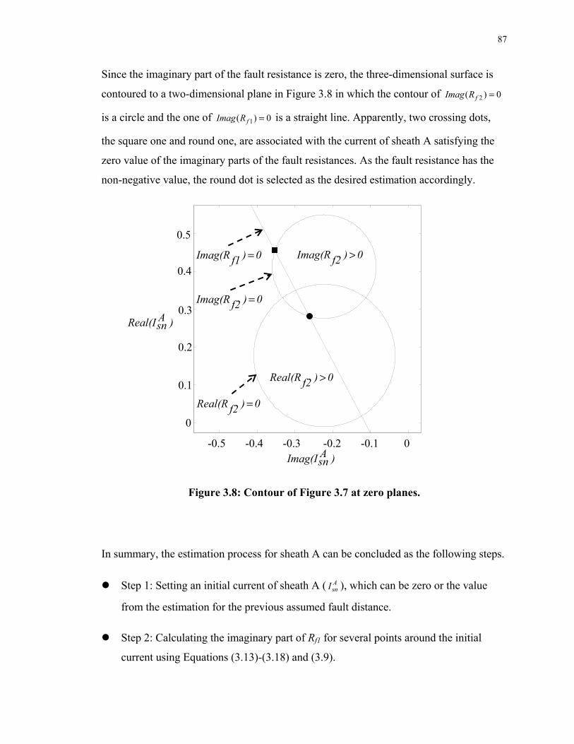
87
Since the imaginary part of the fault resistance is zero, the three-dimensional surface is
contoured to a two-dimensional plane in Figure 3.8 in which the contour of 2( ) 0fImag R =
is a circle and the one of 1( ) 0fImag R = is a straight line. Apparently, two crossing dots,
the square one and round one, are associated with the current of sheath A satisfying the
zero value of the imaginary parts of the fault resistances. As the fault resistance has the
non-negative value, the round dot is selected as the desired estimation accordingly.
Figure 3.8: Contour of Figure 3.7 at zero planes.
In summary, the estimation process for sheath A can be concluded as the following steps.
Step 1: Setting an initial current of sheath A ( AsnI ), which can be zero or the value
from the estimation for the previous assumed fault distance.
Step 2: Calculating the imaginary part of Rf1 for several points around the initial
current using Equations (3.13)-(3.18) and (3.9).
-0.5 -0.4 -0.3 -0.2 -0.1 0
0
0.1
0.2
0.3
0.4
0.5
AReal(I )sn
Imag(R ) 0f2 >Imag(R ) 0f1 =
Imag(R ) 0f2 =
Real(R ) 0f2 =
Real(R ) 0f2 >
AImag(I )sn
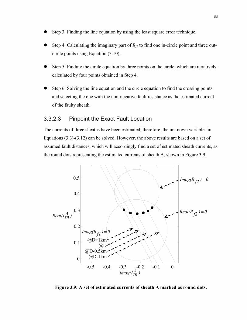
88
Step 3: Finding the line equation by using the least square error technique.
Step 4: Calculating the imaginary part of Rf2 to find one in-circle point and three out-
circle points using Equation (3.10).
Step 5: Finding the circle equation by three points on the circle, which are iteratively
calculated by four points obtained in Step 4.
Step 6: Solving the line equation and the circle equation to find the crossing points
and selecting the one with the non-negative fault resistance as the estimated current
of the faulty sheath.
3.3.2.3 Pinpoint the Exact Fault Location
The currents of three sheaths have been estimated, therefore, the unknown variables in
Equations (3.3)-(3.12) can be solved. However, the above results are based on a set of
assumed fault distances, which will accordingly find a set of estimated sheath currents, as
the round dots representing the estimated currents of sheath A, shown in Figure 3.9.
Figure 3.9: A set of estimated currents of sheath A marked as round dots.
-0.5 -0.4 -0.3 -0.2 -0.1 0
0
0.1
0.2
0.3
0.4
0.5
AReal(I )sn
@D+1km@D
@D-0.5km@D-1km
Imag(R ) 0f2 =
Real(R ) 0f2 =
AImag(I )sn
Imag(R ) 0f1 =
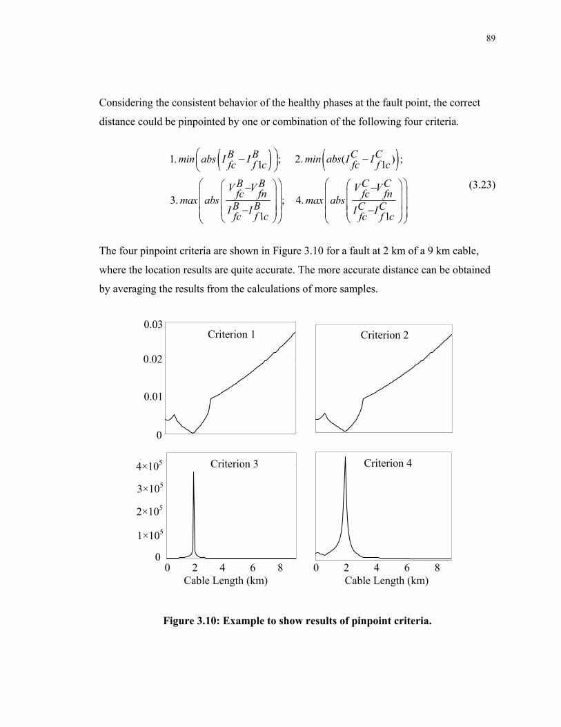
89
Considering the consistent behavior of the healthy phases at the fault point, the correct
distance could be pinpointed by one or combination of the following four criteria.
( ) ( )1 ; 2. ( ) ;1 1
3. ; 4.
1 1
B B C C. min abs I I min abs I Ifc f c fc f c
B B C CV V V Vfc fn fc fn
max abs max absB B C CI I I Ifc f c fc f c
− −
− − − −
(3.23)
The four pinpoint criteria are shown in Figure 3.10 for a fault at 2 km of a 9 km cable,
where the location results are quite accurate. The more accurate distance can be obtained
by averaging the results from the calculations of more samples.
Figure 3.10: Example to show results of pinpoint criteria.
0
0.01
0.02
0.03
0 2 4 6 8 0 2 4 6 8 Cable Length (km) Cable Length (km)
0
1×10⁵
2×10⁵
3×10⁵
4×10⁵
Criterion 1 Criterion 2
Criterion 3 Criterion 4
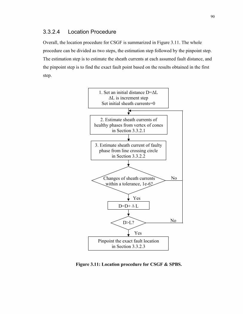
90
3.3.2.4 Location Procedure
Overall, the location procedure for CSGF is summarized in Figure 3.11. The whole
procedure can be divided as two steps, the estimation step followed by the pinpoint step.
The estimation step is to estimate the sheath currents at each assumed fault distance, and
the pinpoint step is to find the exact fault point based on the results obtained in the first
step.
Figure 3.11: Location procedure for CSGF & SPBS.
1. Set an initial distance D=ΔL ΔL is increment step
Set initial sheath currents=0
2. Estimate sheath currents of healthy phases from vertex of cones
in Section 3.3.2.1
Changes of sheath currents within a tolerance, 1e-6?
D=D+ΔL
Pinpoint the exact fault location in Section 3.3.2.3
Yes
No
3. Estimate sheath current of faulty phase from line crossing circle
in Section 3.3.2.2
D>L? No
Yes
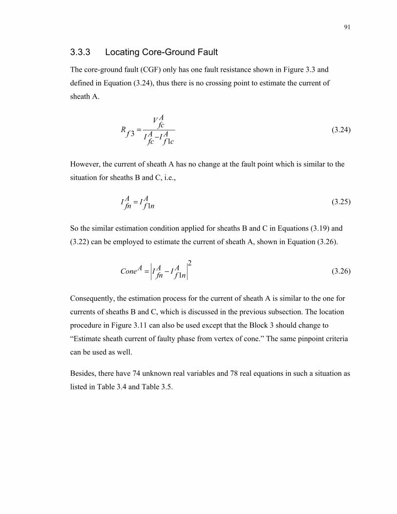
91
3.3.3 Locating Core-Ground Fault
The core-ground fault (CGF) only has one fault resistance shown in Figure 3.3 and
defined in Equation (3.24), thus there is no crossing point to estimate the current of
sheath A.
31
AVfc
R f A AI Ifc f c
=−
(3.24)
However, the current of sheath A has no change at the fault point which is similar to the
situation for sheaths B and C, i.e.,
1A AI Ifn f n= (3.25)
So the similar estimation condition applied for sheaths B and C in Equations (3.19) and
(3.22) can be employed to estimate the current of sheath A, shown in Equation (3.26).
2
1A A ACone I Ifn f n= − (3.26)
Consequently, the estimation process for the current of sheath A is similar to the one for
currents of sheaths B and C, which is discussed in the previous subsection. The location
procedure in Figure 3.11 can also be used except that the Block 3 should change to
“Estimate sheath current of faulty phase from vertex of cone.” The same pinpoint criteria
can be used as well.
Besides, there have 74 unknown real variables and 78 real equations in such a situation as
listed in Table 3.4 and Table 3.5.
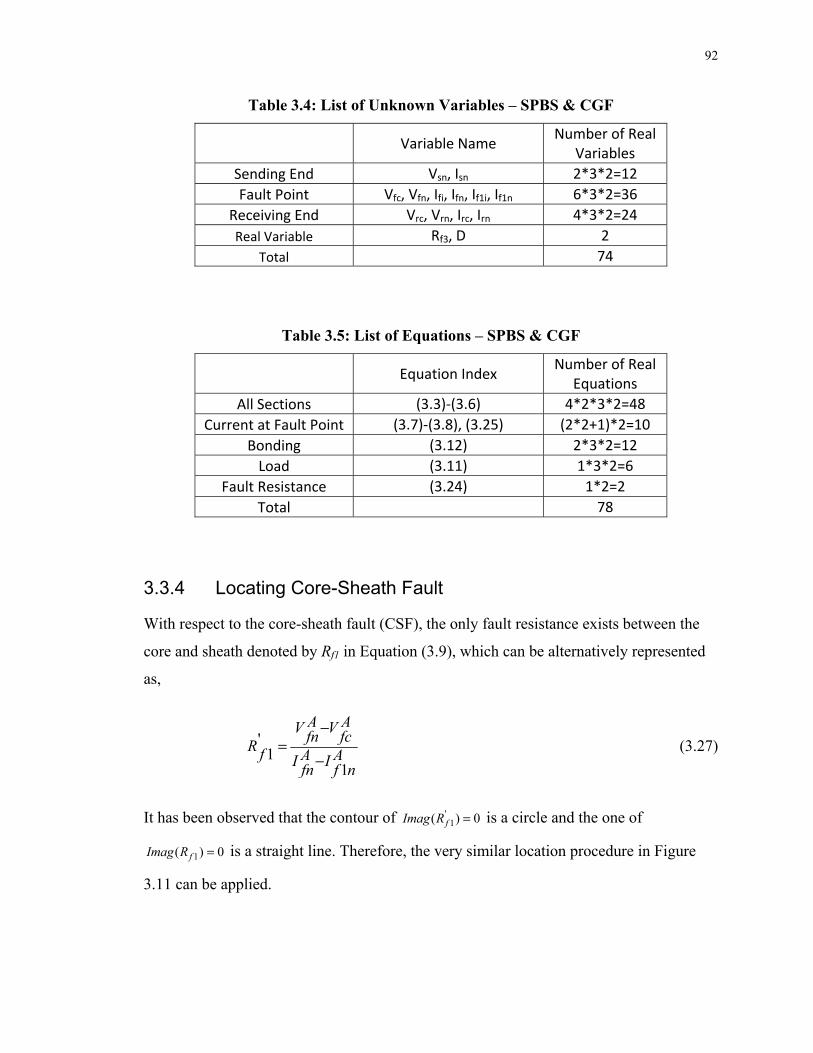
92
Table 3.4: List of Unknown Variables – SPBS & CGF
Variable Name Number of Real Variables
Sending End Vsn, Isn 2*3*2=12 Fault Point Vfc, Vfn, Ifi, Ifn, If1i, If1n 6*3*2=36
Receiving End Vrc, Vrn, Irc, Irn 4*3*2=24 Real Variable Rf3, D 2
Total 74
Table 3.5: List of Equations – SPBS & CGF
Equation Index Number of Real Equations
All Sections (3.3)-(3.6) 4*2*3*2=48 Current at Fault Point (3.7)-(3.8), (3.25) (2*2+1)*2=10
Bonding (3.12) 2*3*2=12 Load (3.11) 1*3*2=6
Fault Resistance (3.24) 1*2=2 Total 78
3.3.4 Locating Core-Sheath Fault
With respect to the core-sheath fault (CSF), the only fault resistance exists between the
core and sheath denoted by Rf1 in Equation (3.9), which can be alternatively represented
as,
'1
1
A AV Vfn fc
R f A AI Ifn f n
−=
− (3.27)
It has been observed that the contour of '1( ) 0fImag R = is a circle and the one of
1( ) 0fImag R = is a straight line. Therefore, the very similar location procedure in Figure
3.11 can be applied.
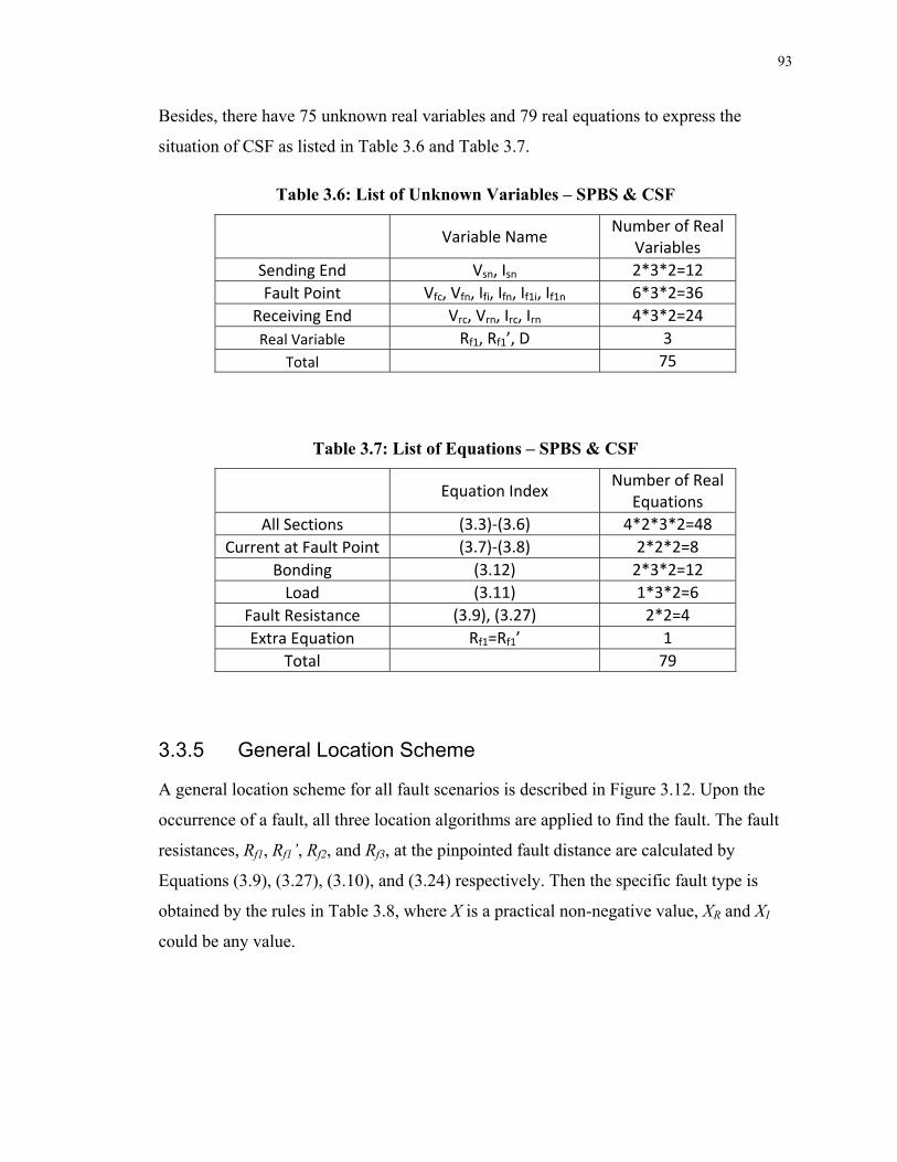
93
Besides, there have 75 unknown real variables and 79 real equations to express the
situation of CSF as listed in Table 3.6 and Table 3.7.
Table 3.6: List of Unknown Variables – SPBS & CSF
Variable Name Number of Real Variables
Sending End Vsn, Isn 2*3*2=12 Fault Point Vfc, Vfn, Ifi, Ifn, If1i, If1n 6*3*2=36
Receiving End Vrc, Vrn, Irc, Irn 4*3*2=24 Real Variable Rf1, Rf1’, D 3
Total 75
Table 3.7: List of Equations – SPBS & CSF
Equation Index Number of Real Equations
All Sections (3.3)-(3.6) 4*2*3*2=48 Current at Fault Point (3.7)-(3.8) 2*2*2=8
Bonding (3.12) 2*3*2=12 Load (3.11) 1*3*2=6
Fault Resistance (3.9), (3.27) 2*2=4 Extra Equation Rf1=Rf1’ 1
Total 79
3.3.5 General Location Scheme
A general location scheme for all fault scenarios is described in Figure 3.12. Upon the
occurrence of a fault, all three location algorithms are applied to find the fault. The fault
resistances, Rf1, Rf1’, Rf2, and Rf3, at the pinpointed fault distance are calculated by
Equations (3.9), (3.27), (3.10), and (3.24) respectively. Then the specific fault type is
obtained by the rules in Table 3.8, where X is a practical non-negative value, XR and XI
could be any value.
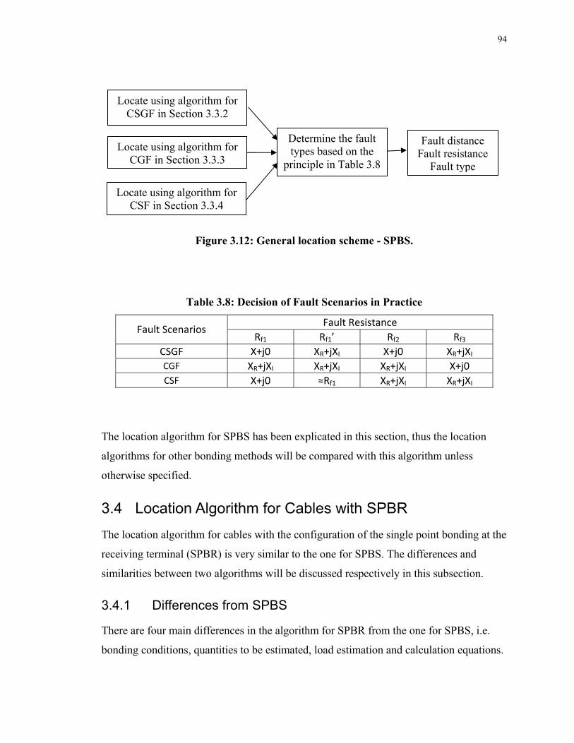
94
Figure 3.12: General location scheme - SPBS.
Table 3.8: Decision of Fault Scenarios in Practice
Fault Resistance Fault Scenarios Rf1 Rf1’ Rf2 Rf3
CSGF X+j0 XR+jXI X+j0 XR+jXI CGF XR+jXI XR+jXI XR+jXI X+j0 CSF X+j0 ≈Rf1 XR+jXI XR+jXI
The location algorithm for SPBS has been explicated in this section, thus the location
algorithms for other bonding methods will be compared with this algorithm unless
otherwise specified.
3.4 Location Algorithm for Cables with SPBR
The location algorithm for cables with the configuration of the single point bonding at the
receiving terminal (SPBR) is very similar to the one for SPBS. The differences and
similarities between two algorithms will be discussed respectively in this subsection.
3.4.1 Differences from SPBS
There are four main differences in the algorithm for SPBR from the one for SPBS, i.e.
bonding conditions, quantities to be estimated, load estimation and calculation equations.
Locate using algorithm for CSGF in Section 3.3.2
Determine the fault types based on the
principle in Table 3.8
Fault distance Fault resistance
Fault type
Locate using algorithm for CGF in Section 3.3.3
Locate using algorithm for CSF in Section 3.3.4
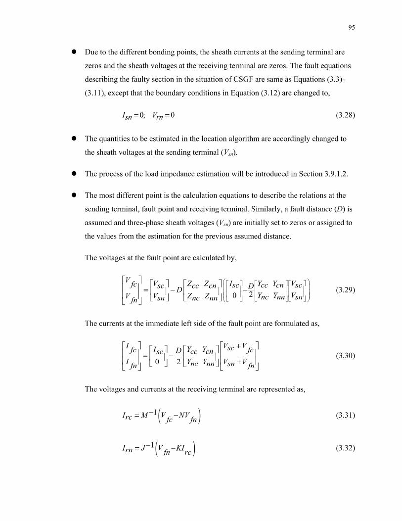
95
Due to the different bonding points, the sheath currents at the sending terminal are
zeros and the sheath voltages at the receiving terminal are zeros. The fault equations
describing the faulty section in the situation of CSGF are same as Equations (3.3)-
(3.11), except that the boundary conditions in Equation (3.12) are changed to,
0; 0I Vsn rn= = (3.28)
The quantities to be estimated in the location algorithm are accordingly changed to
the sheath voltages at the sending terminal (Vsn).
The process of the load impedance estimation will be introduced in Section 3.9.1.2.
The most different point is the calculation equations to describe the relations at the
sending terminal, fault point and receiving terminal. Similarly, a fault distance (D) is
assumed and three-phase sheath voltages (Vsn) are initially set to zeros or assigned to
the values from the estimation for the previous assumed distance.
The voltages at the fault point are calculated by,
20
V V Z Z I Y Y Vfc sc cc cn scsc cc cn DDY Y VV V Z Z nc nn snsn nc nnfn
= − − (3.29)
The currents at the immediate left side of the fault point are formulated as,
20
I V VscY YIfc fcD cc cnscI Y Y V Vnc nn snfn fn
+ = − + (3.30)
The voltages and currents at the receiving terminal are represented as,
( )1I M V NVrc fc fn−= − (3.31)
( )1I J V KIrn fn rc−= − (3.32)
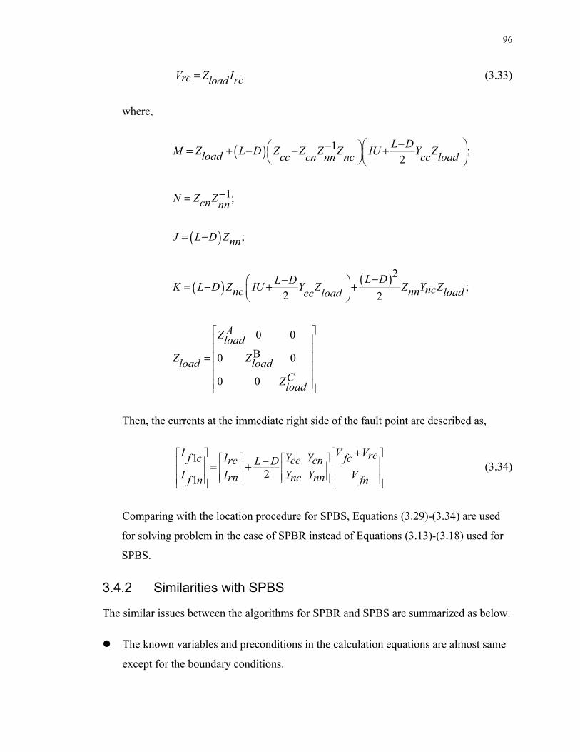
96
V Z Irc rcload= (3.33)
where,
( ) 1 ;2
L DM Z L D Z Z Z Z IU Y Zload cc cn nn nc cc load
− − = + − − +
1;N Z Zcn nn−=
( ) ;J L D Znn= −
( ) ( )2;
2 2
L DL DK L D Z IU Y Z Z Y Zncnc nn loadcc load
−− = − + +
0 0
B0 0
0 0
AZload
Z Zload loadCZload
=
Then, the currents at the immediate right side of the fault point are described as,
1
21
I V VrcI Y Yf c fcrc cc cnL DI I Y Y Vrn nc nnf n fn
+−= + (3.34)
Comparing with the location procedure for SPBS, Equations (3.29)-(3.34) are used
for solving problem in the case of SPBR instead of Equations (3.13)-(3.18) used for
SPBS.
3.4.2 Similarities with SPBS
The similar issues between the algorithms for SPBR and SPBS are summarized as below.
The known variables and preconditions in the calculation equations are almost same
except for the boundary conditions.
97
Similarly, there have 75 unknown real variables and 78 real equations for CSGF &
SPBR, 74 unknown real variables and 78 real equations for CGF & SPBR, and 75
unknown real variables and 79 real equations for CSF & SPBR.
The principle and procedure are basically similar in estimating sheath quantities of
the healthy cables.
The principle and procedure are quite similar in estimating sheath quantities of the
faulty cable.
The pinpoint criteria are completely same.
The location principles for CSF and CGF are similar.
The general location scheme and the fault type decision logic are exactly same.
3.5 Location Algorithm for Cables with SPBM
The cable with sheaths grounded at the middle point (SPBM) can be regarded as two
cable sections, one equivalent to SPBR and the other to SPBS. It is clear that the
algorithms presented in the previous subsections can be respectively applied for each
section. However, the presence of one cable section would affect the calculations for the
other section.
3.5.1 Fault in the First Half Section
3.5.1.1 Problem Formulation
The first half section with SPBM (SPBM-1) can be considered as a cable with SPBR. It is
illustrated in Figure 3.13 where a CSGF occurs in SPBM-1.
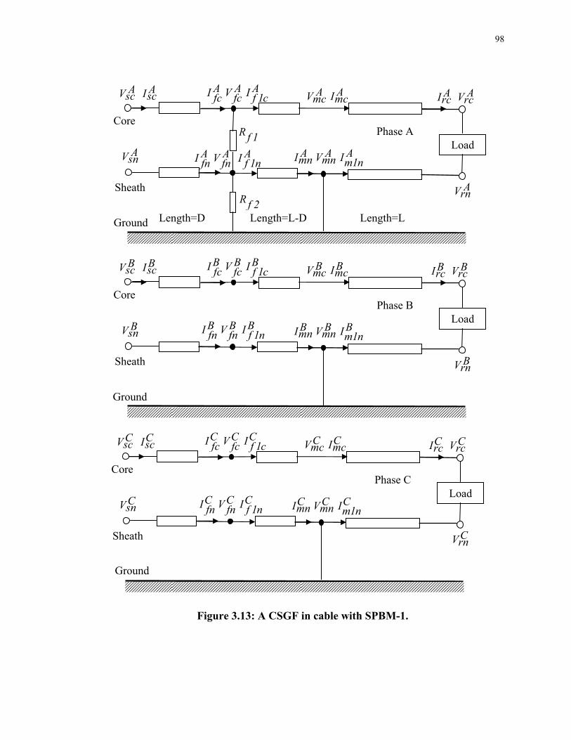
98
Figure 3.13: A CSGF in cable with SPBM-1.
Core
Sheath
Ground
Load Phase A
Length=D Length=L-D Length=L
A AI Vrc rc A A AI V Ifc fc f 1c
A AV Isc sc
AVsn A A AI V Ifn fn f 1n
AVrn
R f 1
R f 2
A AV Imc mc
A A AI V Imn mn m1n
Core
Sheath
Ground
Load Phase B
B BI Vrc rcB B BI V Ifc fc f 1c
B BV Isc sc
BVsn B B BI V Ifn fn f 1n
BVrn
B BV Imc mc
B B BI V Imn mn m1n
Core
Sheath
Ground
Load Phase C
C CI Vrc rcC C CI V Ifc fc f 1c
C CV Isc sc
CVsn C C CI V Ifn fn f 1n
CVrn
C CV Imc mc
C C CI V Imn mn m1n
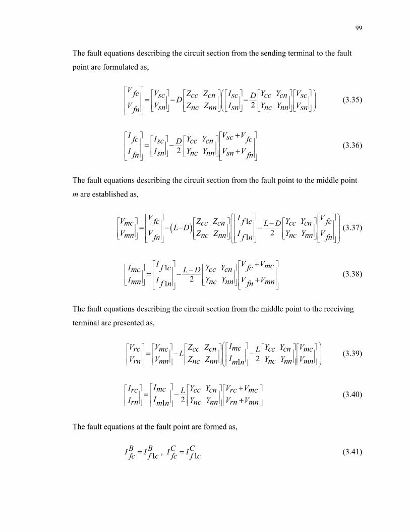
99
The fault equations describing the circuit section from the sending terminal to the fault
point are formulated as,
2
V V Z Z I Y Y Vfc sc cc cn sc cc cn scDDV V Z Z I Y Y Vsn nc nn sn nc nn snfn
= − − (3.35)
2
I V VscI Y Yfc fcsc cc cnDI I Y Y V Vsn nc nn snfn fn
+= −
+ (3.36)
The fault equations describing the circuit section from the fault point to the middle point
m are established as,
( ) 1
21
V I VV Z Z Y Yfc f c fcmc cc cn cc cnL DL DV V Z Z I Y Y Vmn nc nn nc nnfn f n fn
−= − − − (3.37)
1
21
I V VmcI Y Yf c fcmc cc cnL DI I Y Y V Vmn nc nn mnf n fn
+−= −
+ (3.38)
The fault equations describing the circuit section from the middle point to the receiving
terminal are presented as,
21
IV V Z Z Y Y Vmcrc mc cc cn cc cn mcLLIV V Z Z Y Y Vrn mn nc nn nc nn mnm n
= − − (3.39)
21
II Y Y V Vmcrc cc cn rc mcLII Y Y V Vrn nc nn rn mnm n
+= −
+ (3.40)
The fault equations at the fault point are formed as,
,1 1B B C CI I I Ifc f c fc f c= = (3.41)
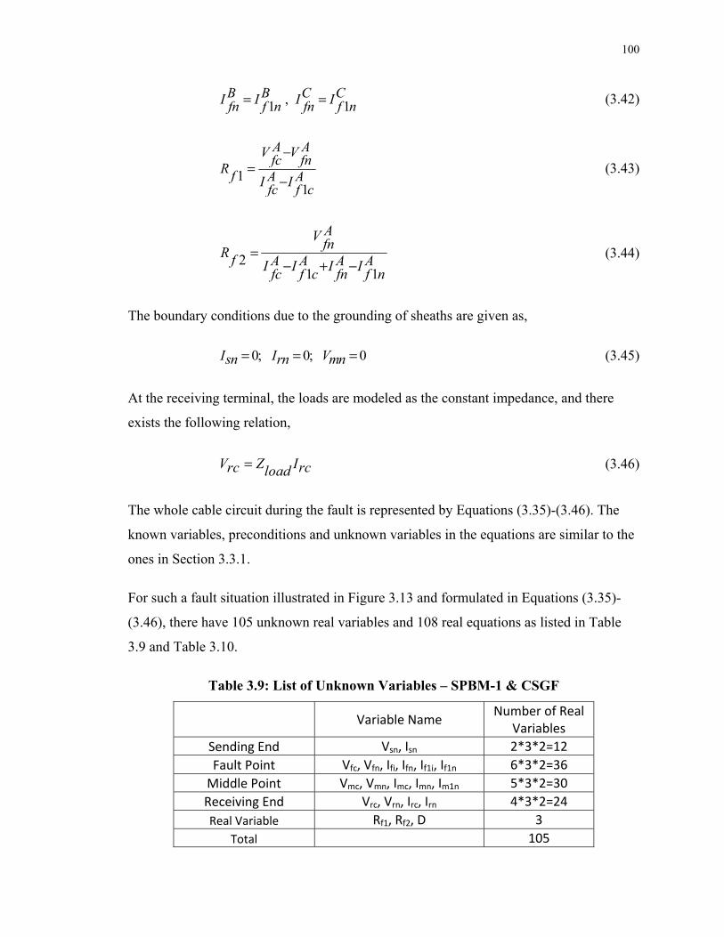
100
,1 1B B C CI I I Ifn f n fn f n= = (3.42)
11
A AV Vfc fn
R f A AI Ifc f c
−=
− (3.43)
21 1
AVfn
R f A A A AI I I Ifc f c fn f n
=− + −
(3.44)
The boundary conditions due to the grounding of sheaths are given as,
0; 0; 0I I Vsn rn mn= = = (3.45)
At the receiving terminal, the loads are modeled as the constant impedance, and there
exists the following relation,
V Z Irc rcload= (3.46)
The whole cable circuit during the fault is represented by Equations (3.35)-(3.46). The
known variables, preconditions and unknown variables in the equations are similar to the
ones in Section 3.3.1.
For such a fault situation illustrated in Figure 3.13 and formulated in Equations (3.35)-
(3.46), there have 105 unknown real variables and 108 real equations as listed in Table
3.9 and Table 3.10.
Table 3.9: List of Unknown Variables – SPBM-1 & CSGF
Variable Name Number of Real Variables
Sending End Vsn, Isn 2*3*2=12 Fault Point Vfc, Vfn, Ifi, Ifn, If1i, If1n 6*3*2=36
Middle Point Vmc, Vmn, Imc, Imn, Im1n 5*3*2=30 Receiving End Vrc, Vrn, Irc, Irn 4*3*2=24 Real Variable Rf1, Rf2, D 3
Total 105
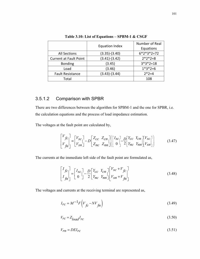
101
Table 3.10: List of Equations – SPBM-1 & CSGF
Equation Index Number of Real Equations
All Sections (3.35)-(3.40) 6*2*3*2=72 Current at Fault Point (3.41)-(3.42) 2*2*2=8
Bonding (3.45) 3*3*2=18 Load (3.46) 1*3*2=6
Fault Resistance (3.43)-(3.44) 2*2=4 Total 108
3.5.1.2 Comparison with SPBR
There are two differences between the algorithm for SPBM-1 and the one for SPBR, i.e.
the calculation equations and the process of load impedance estimation.
The voltages at the fault point are calculated by,
20
V V Z Z I Y Y Vfc sc cc cn scsc cc cn DDY Y VV V Z Z nc nn snsn nc nnfn
= − − (3.47)
The currents at the immediate left side of the fault point are formulated as,
20
I V VscY YIfc fcD cc cnscI Y Y V Vnc nn snfn fn
+ = − + (3.48)
The voltages and currents at the receiving terminal are represented as,
( )1I M F V NVrc fc fn−= − (3.49)
V Z Irc rcload= (3.50)
V DEIrn rc= (3.51)
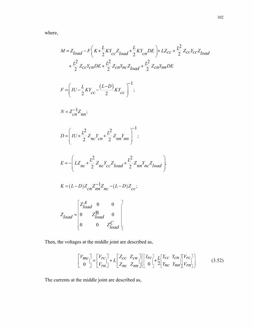
102
where,
2
22 2
2 2 2
2 2 2
L L LM Z F K KY Z KY DE LZ Z Y Zcc cc ccload loadcc load cn
L L LZ Y DE Z Y Z Z Y DEcc cn cn nc cn nnload
= − + + + +
+ + +
( ) 1;
2 2
L DLF IU KY KYcc cc
− −= − −
1 ;N Z Zcn nn−=
12 2;
2 2L L
D IU Z Y Z Ync cn nn nn
− = + +
2 2;
2 2L L
E LZ Z Y Z Z Y Znc nc cc load nn nc load
= − + +
( ) ( )1 ;K L D Z Z Z L D Zcn nn nc cc−= − − −
0 0
B0 0
0 0
AZload
Z Zload loadCZload
=
Then, the voltages at the middle joint are described as,
200
V Z Z I Y Y VV rc cc cn rcrc cc cnmc LLY Y VV Z Z nc nn rnrn nc nn
= + +
(3.52)
The currents at the middle joint are described as,
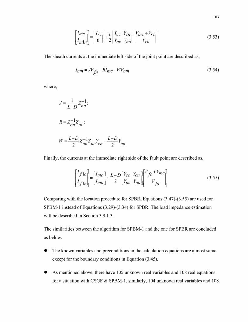
103
201
I Y Y V VImc cc cn mc rcrc LI Y Y Vnc nn rnm n
+= + (3.53)
The sheath currents at the immediate left side of the joint point are described as,
I JV RI WVmn mc mnfn= − − (3.54)
where,
1 1;J ZnnL D−=
−
1 ;R Z Znn nc−=
12 2
L D L DW Z Z Y Ynn nc cn cn
− −−= +
Finally, the currents at the immediate right side of the fault point are described as,
1
21
I V VmcI Y Yf c fcmc cc cnL DI I Y Y Vmn nc nnf n fn
+−= + (3.55)
Comparing with the location procedure for SPBR, Equations (3.47)-(3.55) are used for
SPBM-1 instead of Equations (3.29)-(3.34) for SPBR. The load impedance estimation
will be described in Section 3.9.1.3.
The similarities between the algorithm for SPBM-1 and the one for SPBR are concluded
as below.
The known variables and preconditions in the calculation equations are almost same
except for the boundary conditions in Equation (3.45).
As mentioned above, there have 105 unknown real variables and 108 real equations
for a situation with CSGF & SPBM-1, similarly, 104 unknown real variables and 108
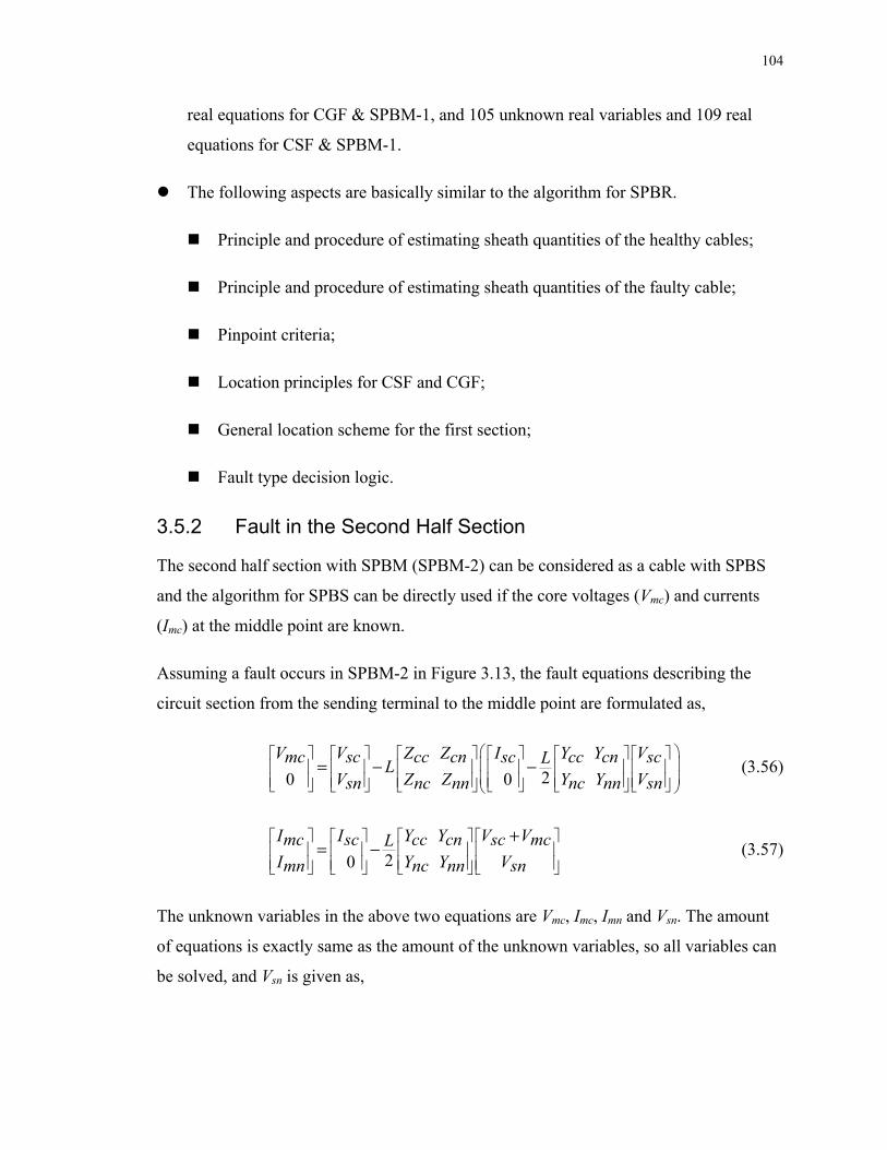
104
real equations for CGF & SPBM-1, and 105 unknown real variables and 109 real
equations for CSF & SPBM-1.
The following aspects are basically similar to the algorithm for SPBR.
Principle and procedure of estimating sheath quantities of the healthy cables;
Principle and procedure of estimating sheath quantities of the faulty cable;
Pinpoint criteria;
Location principles for CSF and CGF;
General location scheme for the first section;
Fault type decision logic.
3.5.2 Fault in the Second Half Section
The second half section with SPBM (SPBM-2) can be considered as a cable with SPBS
and the algorithm for SPBS can be directly used if the core voltages (Vmc) and currents
(Imc) at the middle point are known.
Assuming a fault occurs in SPBM-2 in Figure 3.13, the fault equations describing the
circuit section from the sending terminal to the middle point are formulated as,
20 0
V Z Z Y Y VV Isc cc cn cc cn scmc sc LLV Z Z Y Y Vsn nc nn nc nn sn
= − − (3.56)
20
I Y Y V VImc cc cn sc mcsc LI Y Y Vmn nc nn sn
+= − (3.57)
The unknown variables in the above two equations are Vmc, Imc, Imn and Vsn. The amount
of equations is exactly same as the amount of the unknown variables, so all variables can
be solved, and Vsn is given as,
105
( )1V J MI NVsn sc sc−= − (3.58)
where,
2 2;
2 2L LJ IU Z Y Z Ync cn nn nn= + +
;M LZnc=
2 2
2 2L LN Z Y Z Ync cc nn nc= +
It is obvious that the location problem here is equivalent to the one for SPBS after Vmc
and Imc are estimated by Equations (3.56)-(3.58). Hitherto, the location algorithm for
SPBS in Section 3.3 can be used completely.
3.5.3 Location Scheme for Entire Cable
The location scheme for entire cable is described in Figure 3.14. The first half section is
examined by the algorithm for SPBM-1. If the obtained fault distance (D1) is very close
to the middle point, the algorithm for SPBM-2 is applied then. Otherwise, the distance
D1 is the true fault distance and the location process stops here. If the located distance
(D2) is close to the joint point again, the real fault distance would be around the joint
point. Otherwise, the distance D2 is the true fault distance.
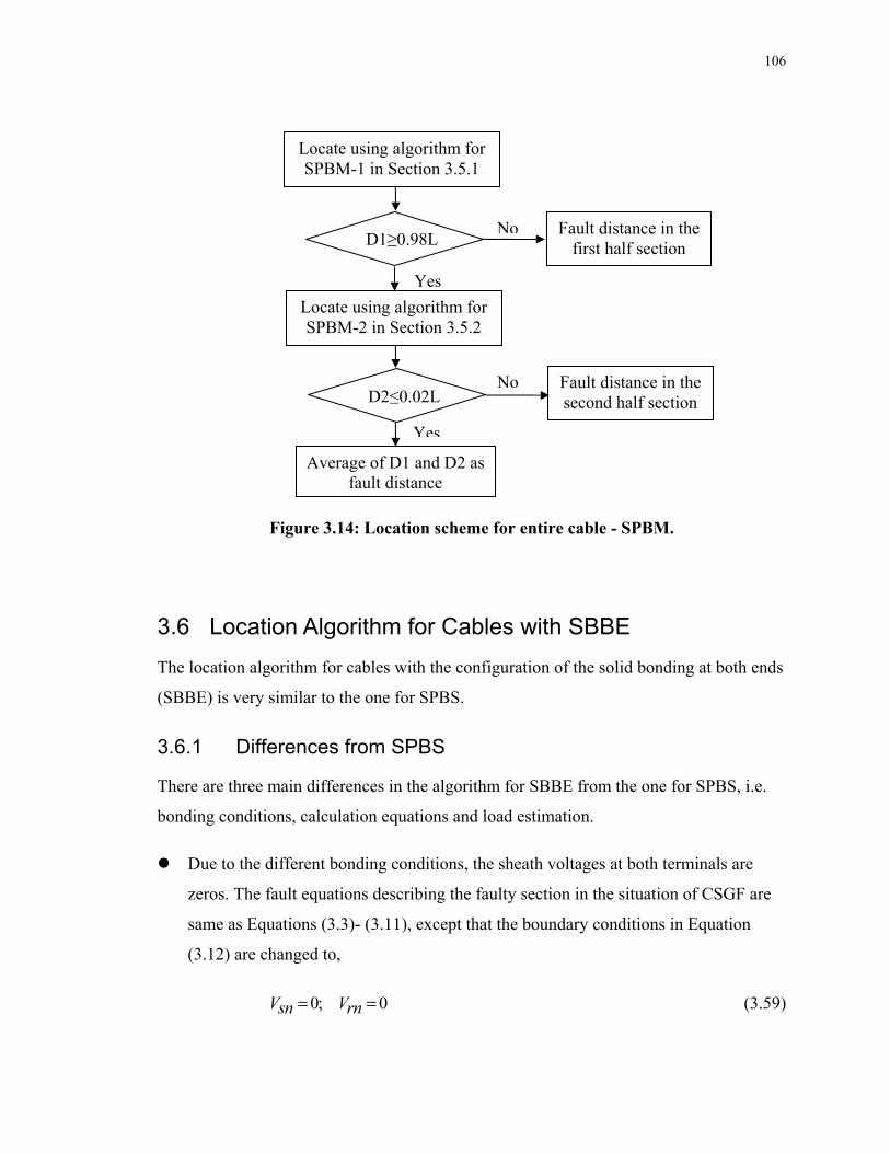
106
Figure 3.14: Location scheme for entire cable - SPBM.
3.6 Location Algorithm for Cables with SBBE
The location algorithm for cables with the configuration of the solid bonding at both ends
(SBBE) is very similar to the one for SPBS.
3.6.1 Differences from SPBS
There are three main differences in the algorithm for SBBE from the one for SPBS, i.e.
bonding conditions, calculation equations and load estimation.
Due to the different bonding conditions, the sheath voltages at both terminals are
zeros. The fault equations describing the faulty section in the situation of CSGF are
same as Equations (3.3)- (3.11), except that the boundary conditions in Equation
(3.12) are changed to,
0; 0V Vsn rn= = (3.59)
Locate using algorithm for SPBM-1 in Section 3.5.1
Fault distance in the first half section
Average of D1 and D2 as fault distance
D1≥0.98L
Yes
No
Locate using algorithm for SPBM-2 in Section 3.5.2
D2≤0.02LNo
Yes
Fault distance in the second half section
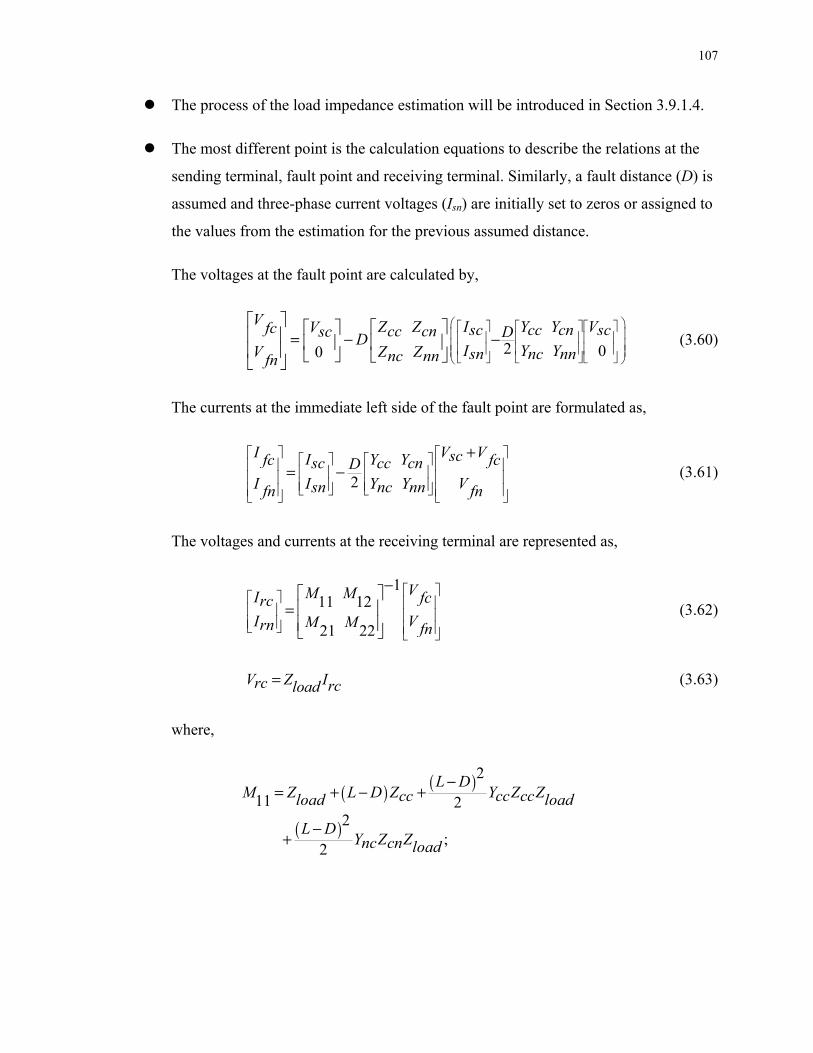
107
The process of the load impedance estimation will be introduced in Section 3.9.1.4.
The most different point is the calculation equations to describe the relations at the
sending terminal, fault point and receiving terminal. Similarly, a fault distance (D) is
assumed and three-phase current voltages (Isn) are initially set to zeros or assigned to
the values from the estimation for the previous assumed distance.
The voltages at the fault point are calculated by,
2 00
V Z Z I Y Y VVfc sc cc cn sccc cnsc DDI Y YV Z Z sn nc nnnc nnfn
= − − (3.60)
The currents at the immediate left side of the fault point are formulated as,
2
I V VscI Y Yfc fcsc cc cnDI I Y Y Vsn nc nnfn fn
+= − (3.61)
The voltages and currents at the receiving terminal are represented as,
111 12
21 22
VM MI fcrcI VM Mrn fn
− =
(3.62)
V Z Irc rcload= (3.63)
where,
( ) ( )
( )
2
11 22
;2
L DM Z L D Z Y Z Zcc cc ccload load
L DY Z Znc cn load
−= + − +
−+
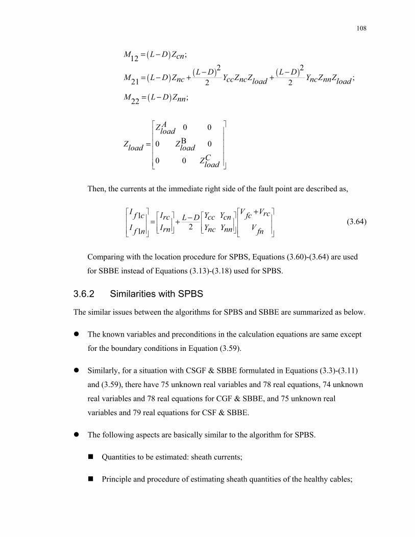
108
( ) ;12M L D Zcn= −
( ) ( ) ( )2 2;21 2 2
L D L DM L D Z Y Z Z Y Z Znc cc nc nc nnload load
− −= − + +
( ) ;22M L D Znn= −
0 0
B0 0
0 0
AZload
Z Zload loadCZload
=
Then, the currents at the immediate right side of the fault point are described as,
1
21
I V VrcI Y Yf c fcrc cc cnL DI I Y Y Vrn nc nnf n fn
+−= + (3.64)
Comparing with the location procedure for SPBS, Equations (3.60)-(3.64) are used
for SBBE instead of Equations (3.13)-(3.18) used for SPBS.
3.6.2 Similarities with SPBS
The similar issues between the algorithms for SPBS and SBBE are summarized as below.
The known variables and preconditions in the calculation equations are same except
for the boundary conditions in Equation (3.59).
Similarly, for a situation with CSGF & SBBE formulated in Equations (3.3)-(3.11)
and (3.59), there have 75 unknown real variables and 78 real equations, 74 unknown
real variables and 78 real equations for CGF & SBBE, and 75 unknown real
variables and 79 real equations for CSF & SBBE.
The following aspects are basically similar to the algorithm for SPBS.
Quantities to be estimated: sheath currents;
Principle and procedure of estimating sheath quantities of the healthy cables;

109
Principle and procedure of estimating sheath quantities of the faulty cable;
Pinpoint criteria;
Location principles for CSF and CGF;
General location scheme;
Fault type decision logic.
3.7 Location Algorithm for Cables with XB
A cable with the cross bonding (XB) is divided into three sections of equal length and the
sheaths are cross-connected at the joints. The first section is similar to SPBS at the
starting terminal of the first section, but there have voltages and currents in sheaths at the
ending terminal of the first section. The middle section has the voltages and currents in
sheaths at both starting and ending terminals of this section. The last section is similar to
SPBR at the ending terminal of the last section, but there have voltages and currents in
sheaths at the starting terminal of the last section.
3.7.1 Fault in the First Section
3.7.1.1 Problem Formulation
A CSGF occurs in the first section with XB (XB-1), as illustrated in Figure 3.15.
The fault equations describing the circuit section from the sending terminal to the fault
point are formulated as,
2
V V Z Z I Y Y Vfc sc cc cn sc cc cn scDDV V Z Z I Y Y Vsn nc nn sn nc nn snfn
= − − (3.65)
2
I V VscI Y Yfc fcsc cc cnDI I Y Y V Vsn nc nn snfn fn
+= −
+ (3.66)
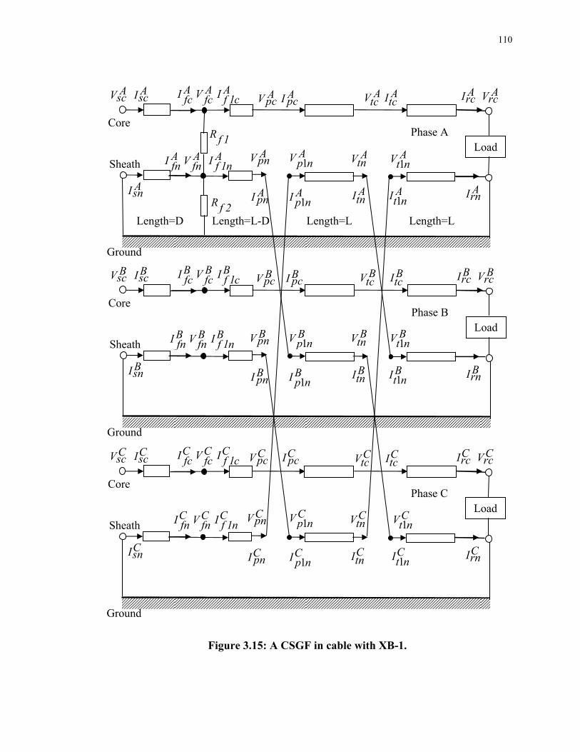
110
Figure 3.15: A CSGF in cable with XB-1.
Core
Sheath
Ground
Load Phase A
Length=D Length=L-D Length=L Length=L
A AI Vrc rcA A AI V Ifc fc f 1c
A AV Isc sc
AIsn
A A AI V Ifn fn f 1n
AIrn
R f 1
R f 2
A AV Ipc pc
1
1
A AV Vpn p n
A AI Ipn p n
1
1
A AV Vtn t n
A AI Itn t n
A AV Itc tc
Core
Sheath
Ground
Load Phase B
B BI Vrc rcB B BI V Ifc fc f 1c
B BV Isc sc
BIsn
B B BI V Ifn fn f 1n
BIrn
B BV Ipc pc
1
1
B BV Vpn p n
B BI Ipn p n
1
1
B BV Vtn t n
B BI Itn t n
B BV Itc tc
C C CI V Ifn fn f 1n 1
1
C CV Vpn p n
C CI Ipn p n
C CV Ipc pc C CV Itc tc
1
1
C CV Vtn t n
C CI Itn t n
Core
Sheath
Ground
Load Phase C
C CI Vrc rcC C CI V Ifc fc f 1c
C CV Isc sc
CIsn CIrn
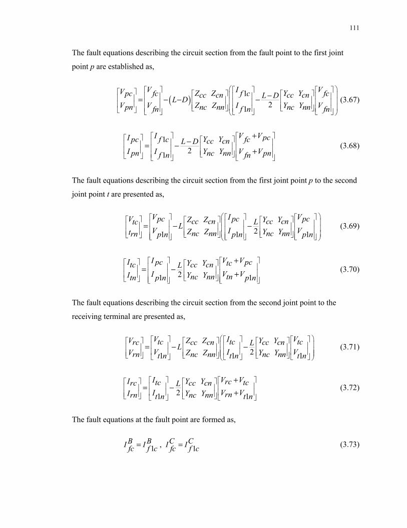
111
The fault equations describing the circuit section from the fault point to the first joint
point p are established as,
( ) 1
21
V I VV Z Z Y Ypc fc f c fccc cn cc cnL DL DV V Z Z I Y Y Vpn nc nn nc nnfn f n fn
−= − − − (3.67)
1
21
I V VpcI Y Ypc f c fccc cnL DI I Y Y V Vpn nc nn pnf n fn
+−= −
+ (3.68)
The fault equations describing the circuit section from the first joint point p to the second
joint point t are presented as,
21 1 1
V I Vpc pc pcV Z Z Y Ycc cn cc cnLtc LV I VZ Z Y Yt nc nn nc nnrn p n p n p n
= − − (3.69)
21 1
I V VI pc pcY Y tctc cc cnLI V VI Y Y tnnc nntn p n p n
+= − + (3.70)
The fault equations describing the circuit section from the second joint point to the
receiving terminal are presented as,
21 1 1
V I VV Z Z Y Ytc tc tcrc cc cn cc cnLLV I VV Z Z Y Yrn nc nn nc nnt n t n t n
= − − (3.71)
21 1
I V VI Y Y rctc tcrc cc cnLI V VI Y Y rnrn nc nnt n t n
+= −
+ (3.72)
The fault equations at the fault point are formed as,
,1 1B B C CI I I Ifc f c fc f c= = (3.73)
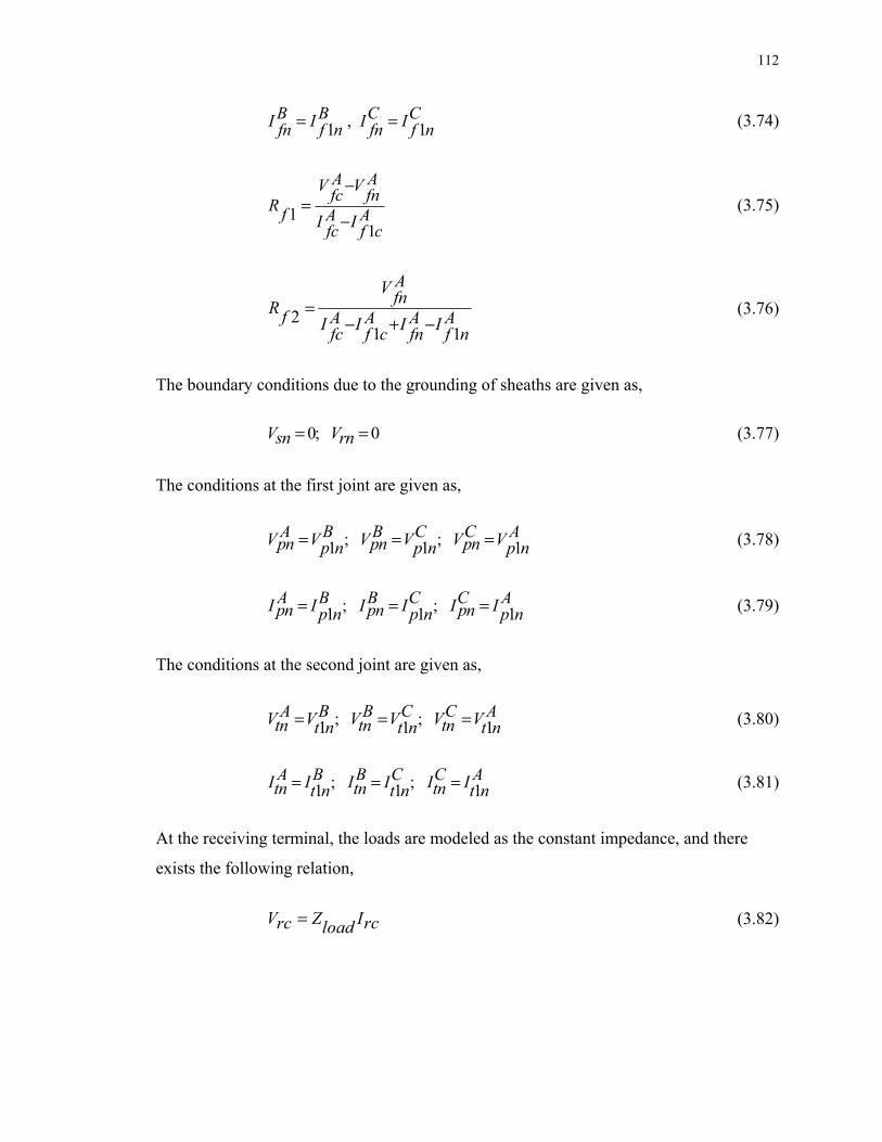
112
,1 1B B C CI I I Ifn f n fn f n= = (3.74)
11
A AV Vfc fn
R f A AI Ifc f c
−=
− (3.75)
21 1
AVfn
R f A A A AI I I Ifc f c fn f n
=− + −
(3.76)
The boundary conditions due to the grounding of sheaths are given as,
0; 0V Vsn rn= = (3.77)
The conditions at the first joint are given as,
; ;1 1 1A B B C C AV V V V V Vpn pn pnp n p n p n= = = (3.78)
; ;1 1 1A B B C C AI I I I I Ipn pn pnp n p n p n= = = (3.79)
The conditions at the second joint are given as,
; ;1 1 1A B B C C AV V V V V Vtn tn tnt n t n t n= = = (3.80)
; ;1 1 1A B B C C AI I I I I Itn tn tnt n t n t n= = = (3.81)
At the receiving terminal, the loads are modeled as the constant impedance, and there
exists the following relation,
V Z Irc rcload= (3.82)
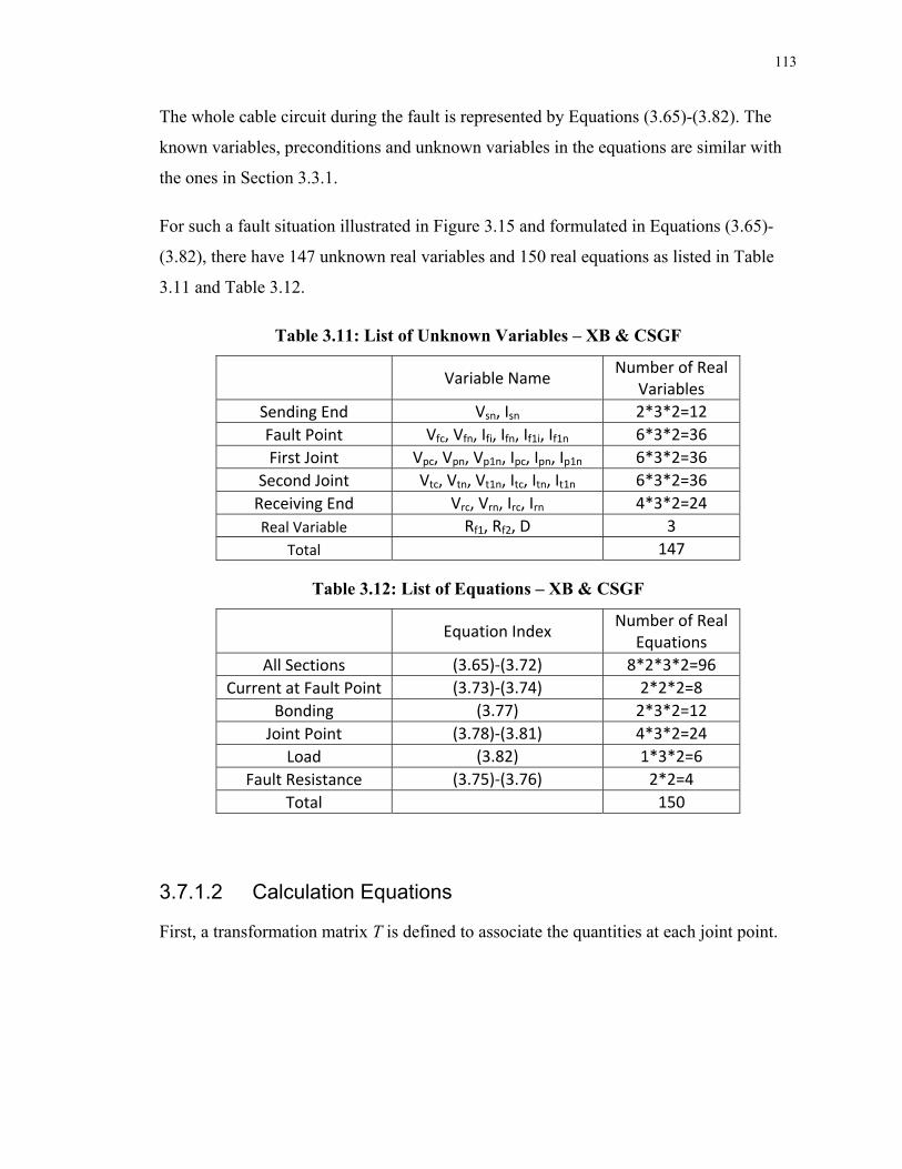
113
The whole cable circuit during the fault is represented by Equations (3.65)-(3.82). The
known variables, preconditions and unknown variables in the equations are similar with
the ones in Section 3.3.1.
For such a fault situation illustrated in Figure 3.15 and formulated in Equations (3.65)-
(3.82), there have 147 unknown real variables and 150 real equations as listed in Table
3.11 and Table 3.12.
Table 3.11: List of Unknown Variables – XB & CSGF
Variable Name Number of Real Variables
Sending End Vsn, Isn 2*3*2=12 Fault Point Vfc, Vfn, Ifi, Ifn, If1i, If1n 6*3*2=36 First Joint Vpc, Vpn, Vp1n, Ipc, Ipn, Ip1n 6*3*2=36
Second Joint Vtc, Vtn, Vt1n, Itc, Itn, It1n 6*3*2=36 Receiving End Vrc, Vrn, Irc, Irn 4*3*2=24 Real Variable Rf1, Rf2, D 3
Total 147
Table 3.12: List of Equations – XB & CSGF
Equation Index Number of Real Equations
All Sections (3.65)-(3.72) 8*2*3*2=96 Current at Fault Point (3.73)-(3.74) 2*2*2=8
Bonding (3.77) 2*3*2=12 Joint Point (3.78)-(3.81) 4*3*2=24
Load (3.82) 1*3*2=6 Fault Resistance (3.75)-(3.76) 2*2=4
Total 150
3.7.1.2 Calculation Equations
First, a transformation matrix T is defined to associate the quantities at each joint point.
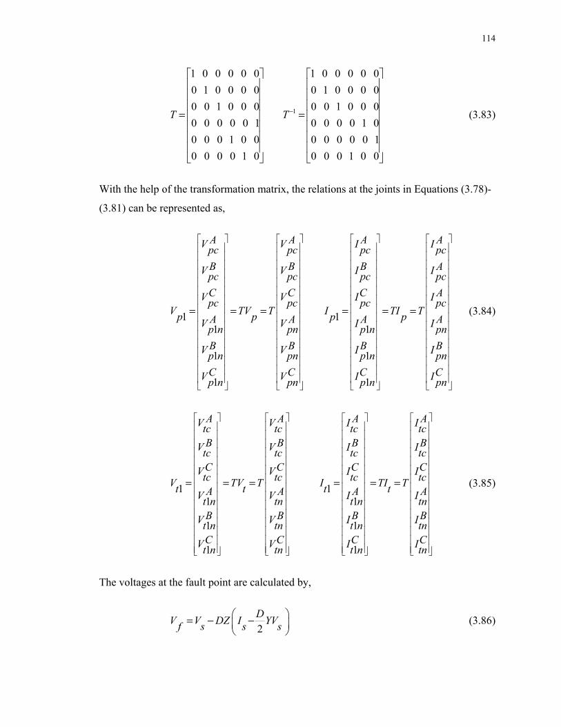
114
1
1 0 0 0 0 0 1 0 0 0 0 0
0 1 0 0 0 0 0 1 0 0 0 0
0 0 1 0 0 0 0 0 1 0 0 0
0 0 0 0 0 1 0 0 0 0 1 0
0 0 0 1 0 0 0 0 0 0 0 1
0 0 0 0 1 0 0 0 0 1 0 0
T T −
= =
(3.83)
With the help of the transformation matrix, the relations at the joints in Equations (3.78)-
(3.81) can be represented as,
1 11 1
1 1
1 1
A A AV V Ipc pc pc
B B BV V Ipc pc pc
C C CV V Ipc pc pcV TV T Ip p pA A AV V Ip n pn p n
B B BV V Ip n pn p n
C C CV V Ip n pn p n
= = = =
AI pc
AI pc
AI pcTI Tp AI pn
BI pn
CI pn
= = (3.84)
1 11 1
1 1
1 1
A A AV V Itc tc tcB B BV V Itc tc tcC C CV V Itc tc tcV TV T I TI Tt t t tA A AV V It n tn t nB B BV V It n tn t nC C CV V It n tn t n
= = = = = =
AItcBItcCItcAItnBItnCItn
(3.85)
The voltages at the fault point are calculated by,
2D
V V DZ I YVf s s s = − −
(3.86)
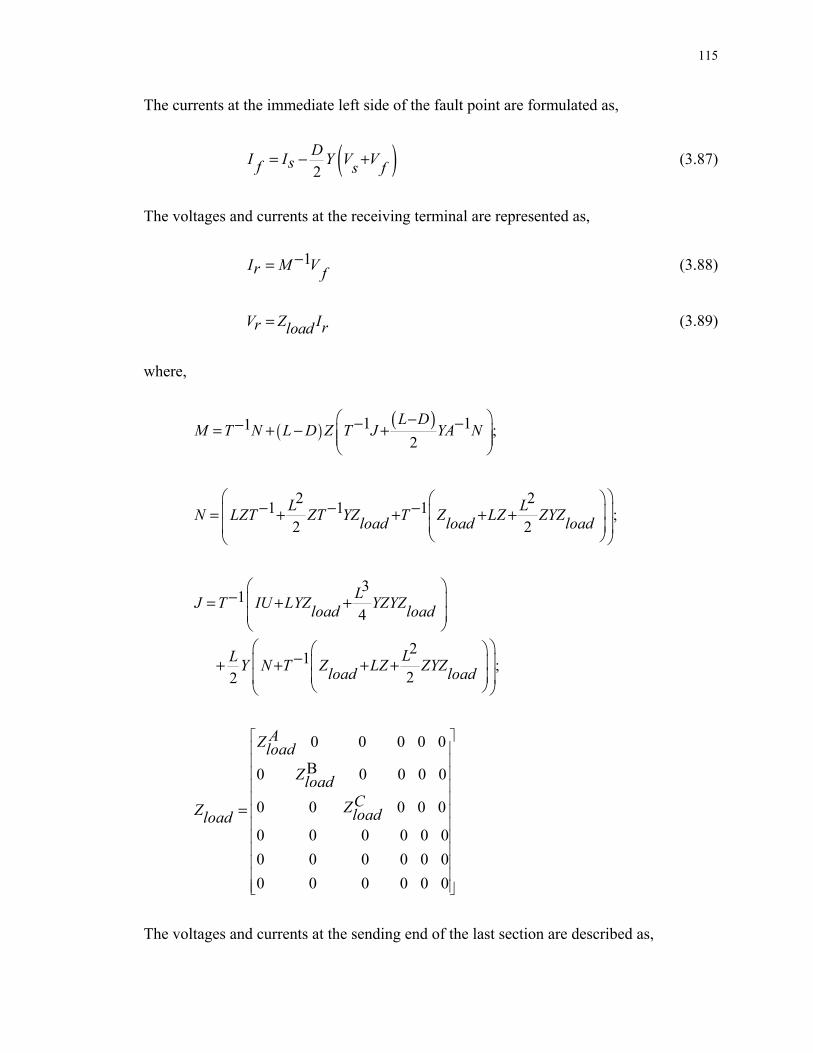
115
The currents at the immediate left side of the fault point are formulated as,
( )2D
I I Y V Vsf s f= − + (3.87)
The voltages and currents at the receiving terminal are represented as,
1I M Vr f−= (3.88)
V Z Ir rload= (3.89)
where,
( ) ( )1 11 ;2
L DM T N L D Z T J YA N
−− −−= + − +
2 21 1 1 ;
2 2L L
N LZT ZT YZ T Z LZ ZYZload load load
− − − = + + + +
31
4
21 ;
22
LJ T IU LYZ YZYZload load
LLY N T Z LZ ZYZload load
− = + + − + + + +
0 0 0 0 0
B0 0 0 0 0
0 0 0 0 0
0 0 0 0 0 0
0 0 0 0 0 0
0 0 0 0 0 0
AZload
ZloadCZZ loadload
=
The voltages and currents at the sending end of the last section are described as,
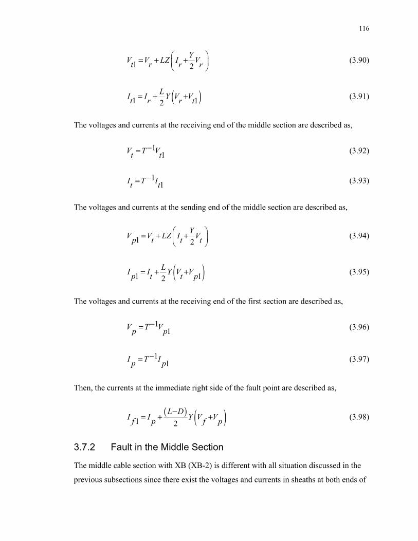
116
1 2Y
V V LZ I Vt r r r = + +
(3.90)
( )1 12L
I I Y V Vt r r t= + + (3.91)
The voltages and currents at the receiving end of the middle section are described as,
11V T Vt t
−= (3.92)
11I T It t
−= (3.93)
The voltages and currents at the sending end of the middle section are described as,
1 2Y
V V LZ I Vp t t t = + +
(3.94)
( )1 12L
I I Y V Vp t t p= + + (3.95)
The voltages and currents at the receiving end of the first section are described as,
11V T Vp p
−= (3.96)
11I T Ip p
−= (3.97)
Then, the currents at the immediate right side of the fault point are described as,
( ) ( )1 2
L DI I Y V Vf p f p
−= + + (3.98)
3.7.2 Fault in the Middle Section
The middle cable section with XB (XB-2) is different with all situation discussed in the
previous subsections since there exist the voltages and currents in sheaths at both ends of
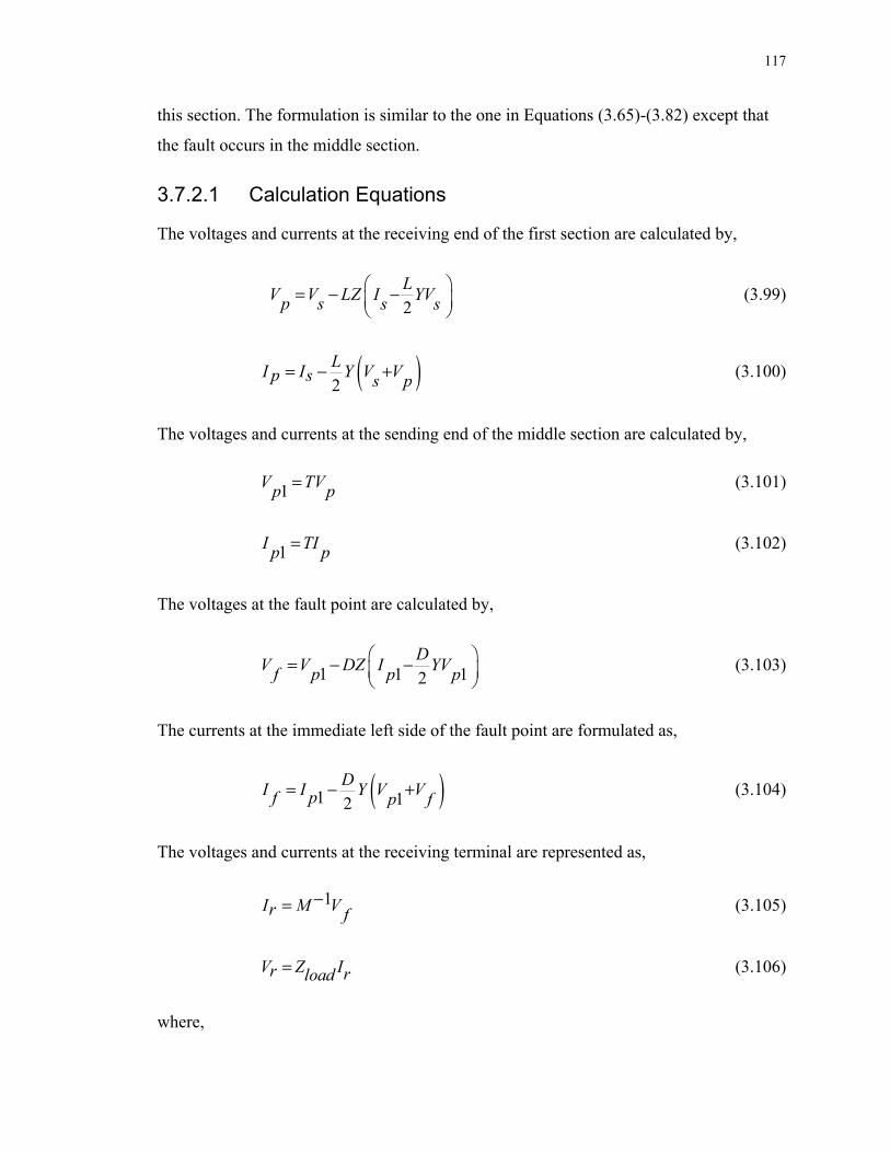
117
this section. The formulation is similar to the one in Equations (3.65)-(3.82) except that
the fault occurs in the middle section.
3.7.2.1 Calculation Equations
The voltages and currents at the receiving end of the first section are calculated by,
2L
V V LZ I YVp s s s = − −
(3.99)
( )2L
I I Y V Vp s s p= − + (3.100)
The voltages and currents at the sending end of the middle section are calculated by,
1V TVp p= (3.101)
1I TIp p= (3.102)
The voltages at the fault point are calculated by,
1 1 12D
V V DZ I YVf p p p = − −
(3.103)
The currents at the immediate left side of the fault point are formulated as,
( )1 12D
I I Y V Vpf p f= − + (3.104)
The voltages and currents at the receiving terminal are represented as,
1I M Vr f−= (3.105)
V Z Ir rload= (3.106)
where,
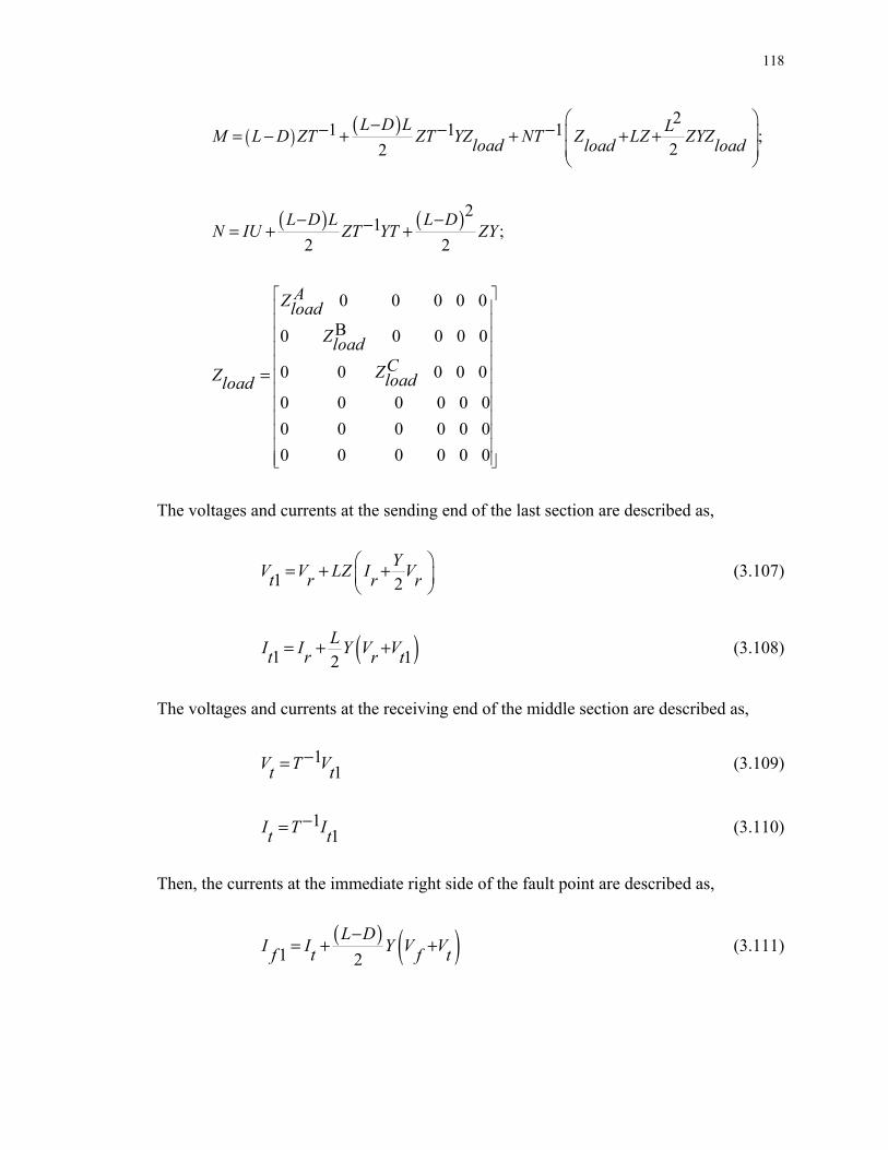
118
( ) ( ) 21 1 1 ;
22
L D L LM L D ZT ZT YZ NT Z LZ ZYZload load load
−− − − = − + + + +
( ) ( )21 ;2 2
L D L L DN IU ZT YT ZY
− −−= + +
0 0 0 0 0
B0 0 0 0 0
0 0 0 0 0
0 0 0 0 0 0
0 0 0 0 0 0
0 0 0 0 0 0
AZload
ZloadCZZ loadload
=
The voltages and currents at the sending end of the last section are described as,
1 2Y
V V LZ I Vt r r r = + +
(3.107)
( )1 12L
I I Y V Vt r r t= + + (3.108)
The voltages and currents at the receiving end of the middle section are described as,
11V T Vt t
−= (3.109)
11I T It t
−= (3.110)
Then, the currents at the immediate right side of the fault point are described as,
( ) ( )1 2
L DI I Y V Vf t f t
−= + + (3.111)
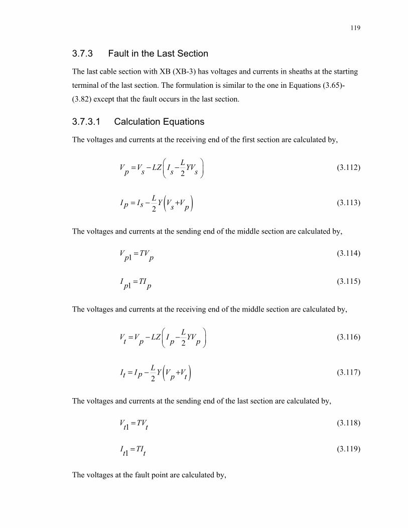
119
3.7.3 Fault in the Last Section
The last cable section with XB (XB-3) has voltages and currents in sheaths at the starting
terminal of the last section. The formulation is similar to the one in Equations (3.65)-
(3.82) except that the fault occurs in the last section.
3.7.3.1 Calculation Equations
The voltages and currents at the receiving end of the first section are calculated by,
2L
V V LZ I YVp s s s = − −
(3.112)
( )2L
I I Y V Vp s s p= − + (3.113)
The voltages and currents at the sending end of the middle section are calculated by,
1V TVp p= (3.114)
1I TIp p= (3.115)
The voltages and currents at the receiving end of the middle section are calculated by,
2L
V V LZ I YVt p p p = − −
(3.116)
( )2L
I I Y V Vpt p t= − + (3.117)
The voltages and currents at the sending end of the last section are calculated by,
1V TVt t= (3.118)
1I TIt t= (3.119)
The voltages at the fault point are calculated by,
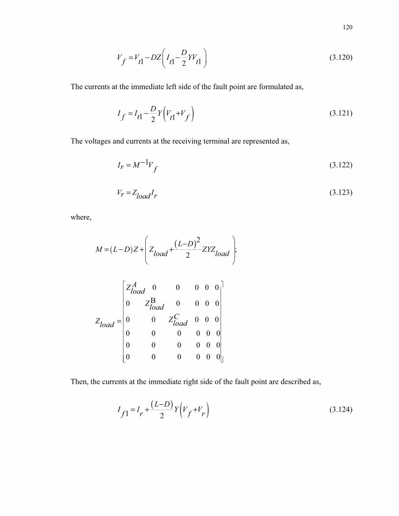
120
1 1 12D
V V DZ I YVf t t t = − −
(3.120)
The currents at the immediate left side of the fault point are formulated as,
( )1 12D
I I Y V Vtf t f= − + (3.121)
The voltages and currents at the receiving terminal are represented as,
1I M Vr f−= (3.122)
V Z Ir rload= (3.123)
where,
( ) ( )2;
2
L DM L D Z Z ZYZload load
− = − + +
0 0 0 0 0
B0 0 0 0 0
0 0 0 0 0
0 0 0 0 0 0
0 0 0 0 0 0
0 0 0 0 0 0
AZload
ZloadCZZ loadload
=
Then, the currents at the immediate right side of the fault point are described as,
( ) ( )1 2
L DI I Y V Vf r f r
−= + + (3.124)

121
3.7.4 Other Issues
Comparing with the detailed principle and procedure for SPBS, the similarity issues for
all three XB methods are summarized as below.
The known variables and preconditions in the calculation equations are same except
for the boundary conditions in Equation (3.77).
There have 147 unknown real variables and 150 real equations for CSGF & XB, 146
unknown real variables and 150 real equations for CGF & XB, and 147 unknown
real variables and 151 real equations for CSF & XB.
The following aspects are basically similar to the algorithm for SPBS.
Quantities to be estimated: sheath currents;
Principle and procedure of estimating sheath quantities of the healthy cables;
Principle and procedure of estimating sheath quantities of the faulty cable;
Pinpoint criteria;
Location principles for CSF and CGF;
General location scheme for each section
Fault type decision logic.
Besides, the process of the load impedance estimation will be introduced in Section
3.9.1.5.
3.7.5 Location Scheme for Entire Cable
Similar to the location scheme for SPBM, the location scheme for entire cable with XB is
described in Figure 3.16.
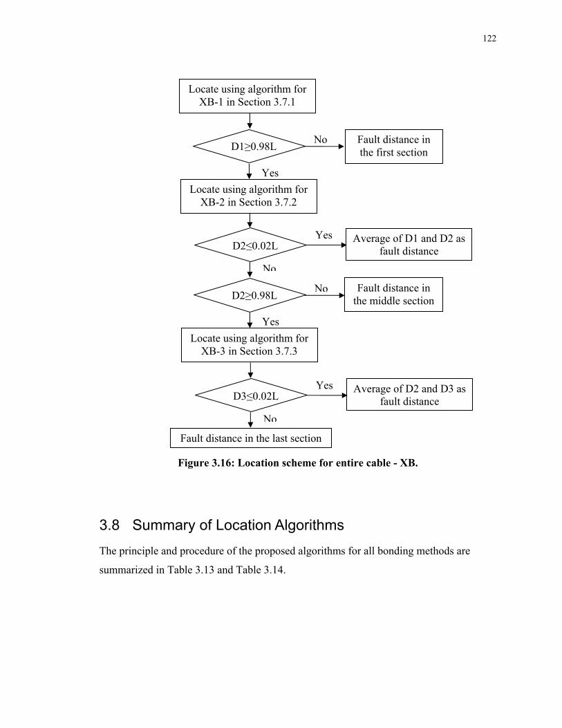
122
Figure 3.16: Location scheme for entire cable - XB.
3.8 Summary of Location Algorithms
The principle and procedure of the proposed algorithms for all bonding methods are
summarized in Table 3.13 and Table 3.14.
Locate using algorithm for XB-1 in Section 3.7.1
Fault distance in the first section
Average of D1 and D2 as fault distance
D1≥0.98L
No
No
Locate using algorithm for XB-2 in Section 3.7.2
D2≤0.02L
Yes
Fault distance in the middle section D2≥0.98L
No
Yes
Yes
Locate using algorithm for XB-3 in Section 3.7.3
Average of D2 and D3 as fault distance
No
D3≤0.02LYes
Fault distance in the last section
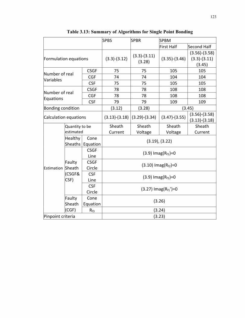
123
Table 3.13: Summary of Algorithms for Single Point Bonding
SPBM SPBS SPBR
First Half Second Half
Formulation equations (3.3)-(3.12) (3.3)-(3.11) (3.28) (3.35)-(3.46)
(3.56)-(3.58)(3.3)-(3.11)
(3.45) CSGF 75 75 105 105 CGF 74 74 104 104 Number of real
Variables CSF 75 75 105 105
CSGF 78 78 108 108 CGF 78 78 108 108 Number of real
Equations CSF 79 79 109 109
Bonding condition (3.12) (3.28) (3.45)
Calculation equations (3.13)-(3.18) (3.29)-(3.34) (3.47)-(3.55) (3.56)-(3.58)(3.13)-(3.18)
Quantity to be estimated
Sheath Current
Sheath Voltage
Sheath Voltage
Sheath Current
Healthy Sheaths
Cone Equation (3.19), (3.22)
CSGF Line (3.9) Imag(Rf1)=0
CSGF Circle (3.10) Imag(Rf2)=0
CSF Line (3.9) Imag(Rf1)=0
Faulty Sheath (CSGF&CSF)
CSF Circle (3.27) Imag(Rf1’)=0
Cone Equation (3.26)
Estimation
Faulty Sheath (CGF) Rf3 (3.24)
Pinpoint criteria (3.23)
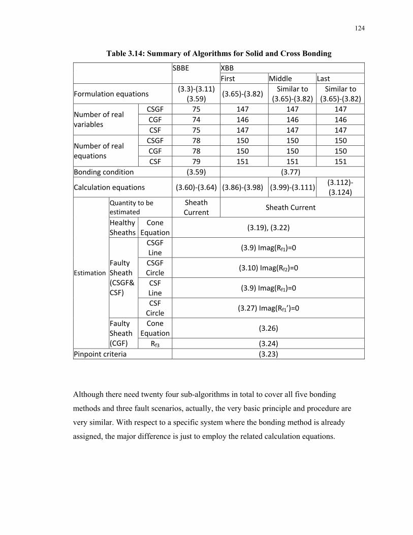
124
Table 3.14: Summary of Algorithms for Solid and Cross Bonding
XBB
SBBE First Middle Last
Formulation equations (3.3)-(3.11) (3.59) (3.65)-(3.82) Similar to
(3.65)-(3.82) Similar to
(3.65)-(3.82)CSGF 75 147 147 147 CGF 74 146 146 146 Number of real
variables CSF 75 147 147 147
CSGF 78 150 150 150 CGF 78 150 150 150 Number of real
equations CSF 79 151 151 151
Bonding condition (3.59) (3.77)
Calculation equations (3.60)-(3.64) (3.86)-(3.98) (3.99)-(3.111) (3.112)-(3.124)
Quantity to be estimated
Sheath Current Sheath Current
Healthy Sheaths
Cone Equation (3.19), (3.22)
CSGF Line (3.9) Imag(Rf1)=0
CSGF Circle (3.10) Imag(Rf2)=0
CSF Line (3.9) Imag(Rf1)=0
Faulty Sheath (CSGF&CSF)
CSF Circle (3.27) Imag(Rf1’)=0
Cone Equation (3.26)
Estimation
Faulty Sheath (CGF) Rf3 (3.24)
Pinpoint criteria (3.23)
Although there need twenty four sub-algorithms in total to cover all five bonding
methods and three fault scenarios, actually, the very basic principle and procedure are
very similar. With respect to a specific system where the bonding method is already
assigned, the major difference is just to employ the related calculation equations.
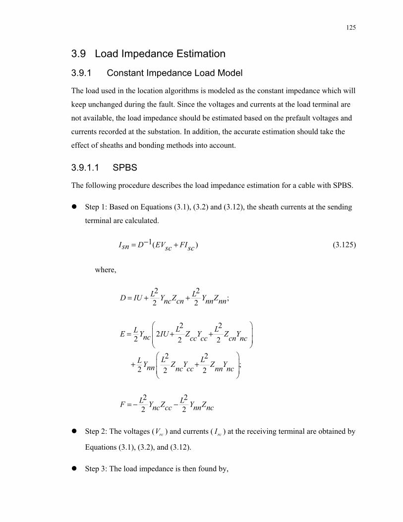
125
3.9 Load Impedance Estimation
3.9.1 Constant Impedance Load Model
The load used in the location algorithms is modeled as the constant impedance which will
keep unchanged during the fault. Since the voltages and currents at the load terminal are
not available, the load impedance should be estimated based on the prefault voltages and
currents recorded at the substation. In addition, the accurate estimation should take the
effect of sheaths and bonding methods into account.
3.9.1.1 SPBS
The following procedure describes the load impedance estimation for a cable with SPBS.
Step 1: Based on Equations (3.1), (3.2) and (3.12), the sheath currents at the sending
terminal are calculated.
1( )I D EV FIsn sc sc−= + (3.125)
where,
2 2;
2 2L LD IU Y Z Y Znc cn nn nn= + +
2 22
2 2 2
2 2;
2 2 2
L LLE Y IU Z Y Z Ync cc cc cn nc
L LL Y Z Y Z Ynn nc cc nn nc
= + + + +
2 2
2 2L LF Y Z Y Znc cc nn nc= − −
Step 2: The voltages ( rcV ) and currents ( rcI ) at the receiving terminal are obtained by
Equations (3.1), (3.2), and (3.12).
Step 3: The load impedance is then found by,
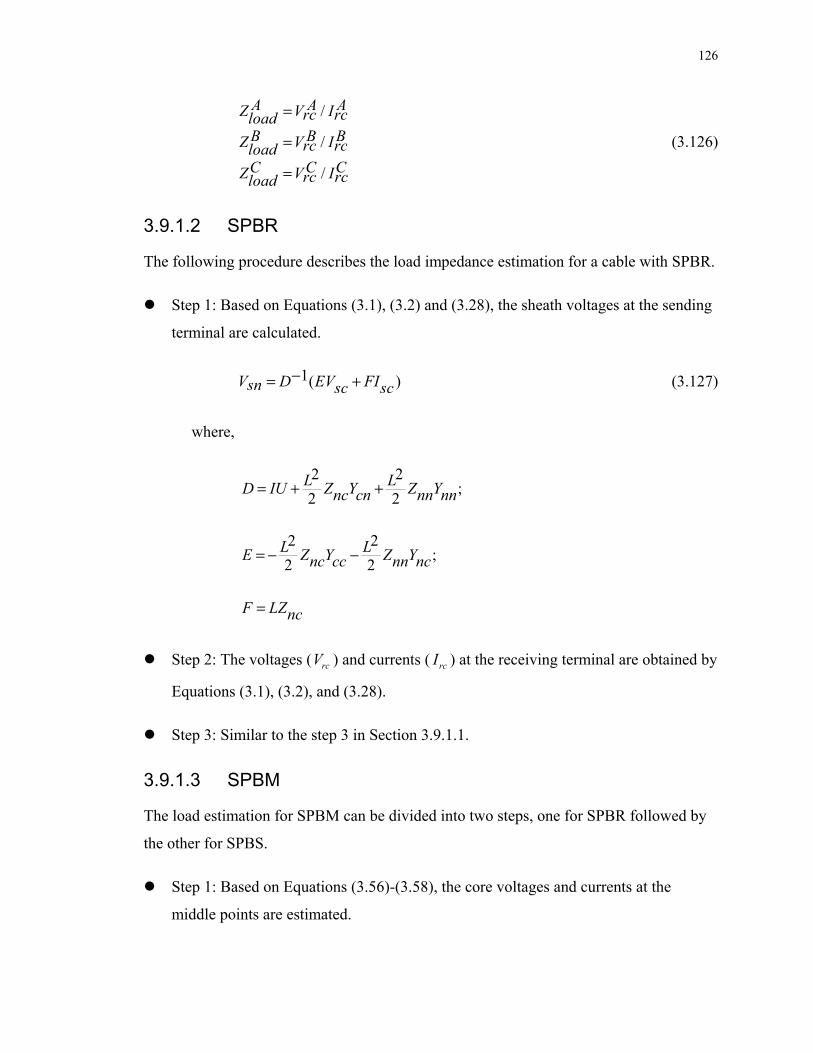
126
/
/
/
A A AZ V Irc rcloadB B BZ V Irc rcloadC C CZ V Irc rcload
=
=
=
(3.126)
3.9.1.2 SPBR
The following procedure describes the load impedance estimation for a cable with SPBR.
Step 1: Based on Equations (3.1), (3.2) and (3.28), the sheath voltages at the sending
terminal are calculated.
1( )V D EV FIsn sc sc−= + (3.127)
where,
2 2;
2 2L LD IU Z Y Z Ync cn nn nn= + +
2 2;
2 2L LE Z Y Z Ync cc nn nc= − −
F LZnc=
Step 2: The voltages ( rcV ) and currents ( rcI ) at the receiving terminal are obtained by
Equations (3.1), (3.2), and (3.28).
Step 3: Similar to the step 3 in Section 3.9.1.1.
3.9.1.3 SPBM
The load estimation for SPBM can be divided into two steps, one for SPBR followed by
the other for SPBS.
Step 1: Based on Equations (3.56)-(3.58), the core voltages and currents at the
middle points are estimated.
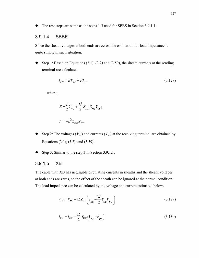
127
The rest steps are same as the steps 1-3 used for SPBS in Section 3.9.1.1.
3.9.1.4 SBBE
Since the sheath voltages at both ends are zeros, the estimation for load impedance is
quite simple in such situation.
Step 1: Based on Equations (3.1), (3.2) and (3.59), the sheath currents at the sending
terminal are calculated.
I EV FIsn sc sc= + (3.128)
where,
3;
2 2L LE Y Z Z Ync nn nc cc= +
2F L Z Znn nc= −
Step 2: The voltages ( rcV ) and currents ( rcI ) at the receiving terminal are obtained by
Equations (3.1), (3.2), and (3.59).
Step 3: Similar to the step 3 in Section 3.9.1.1.
3.9.1.5 XB
The cable with XB has negligible circulating currents in sheaths and the sheath voltages
at both ends are zeros, so the effect of the sheath can be ignored at the normal condition.
The load impedance can be calculated by the voltage and current estimated below.
33
2L
V V LZ I Y Vrc sc cc sc cc sc = − −
(3.129)
( )32L
I I Y V Vrc sc cc sc rc= − + (3.130)
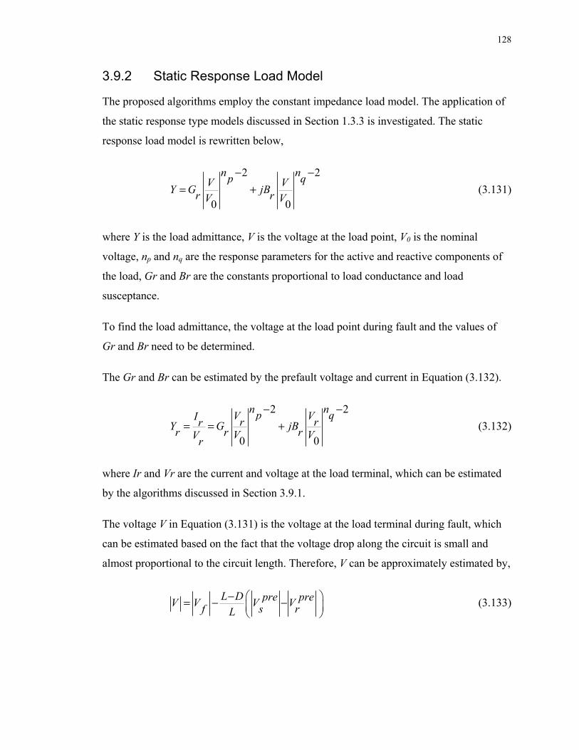
128
3.9.2 Static Response Load Model
The proposed algorithms employ the constant impedance load model. The application of
the static response type models discussed in Section 1.3.3 is investigated. The static
response load model is rewritten below,
2 2
0 0
n np qV VY G jBr rV V
− −= + (3.131)
where Y is the load admittance, V is the voltage at the load point, V0 is the nominal
voltage, np and nq are the response parameters for the active and reactive components of
the load, Gr and Br are the constants proportional to load conductance and load
susceptance.
To find the load admittance, the voltage at the load point during fault and the values of
Gr and Br need to be determined.
The Gr and Br can be estimated by the prefault voltage and current in Equation (3.132).
2 2
0 0
n np qV VI r rrY G jBr r rV VVr
− −= = + (3.132)
where Ir and Vr are the current and voltage at the load terminal, which can be estimated
by the algorithms discussed in Section 3.9.1.
The voltage V in Equation (3.131) is the voltage at the load terminal during fault, which
can be estimated based on the fact that the voltage drop along the circuit is small and
almost proportional to the circuit length. Therefore, V can be approximately estimated by,
L D pre preV V V Vf s rL− = − −
(3.133)
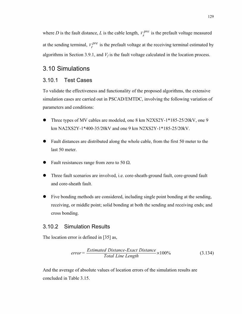
129
where D is the fault distance, L is the cable length, preVs is the prefault voltage measured
at the sending terminal, preVr is the prefault voltage at the receiving terminal estimated by
algorithms in Section 3.9.1, and Vf is the fault voltage calculated in the location process.
3.10 Simulations
3.10.1 Test Cases
To validate the effectiveness and functionality of the proposed algorithms, the extensive
simulation cases are carried out in PSCAD/EMTDC, involving the following variation of
parameters and conditions:
Three types of MV cables are modeled, one 8 km N2XS2Y-1*185-25/20kV, one 9
km NA2XS2Y-1*400-35/20kV and one 9 km N2XS2Y-1*185-25/20kV.
Fault distances are distributed along the whole cable, from the first 50 meter to the
last 50 meter.
Fault resistances range from zero to 50 Ω.
Three fault scenarios are involved, i.e. core-sheath-ground fault, core-ground fault
and core-sheath fault.
Five bonding methods are considered, including single point bonding at the sending,
receiving, or middle point; solid bonding at both the sending and receiving ends; and
cross bonding.
3.10.2 Simulation Results
The location error is defined in [35] as,
100%Estimated Distance-Exact Distance
error =Total Line Length
× (3.134)
And the average of absolute values of location errors of the simulation results are
concluded in Table 3.15.
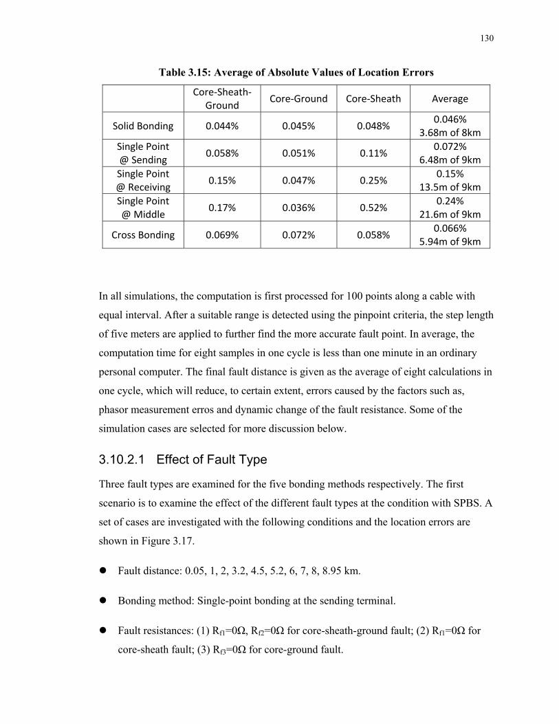
130
Table 3.15: Average of Absolute Values of Location Errors
Core-Sheath- Ground Core-Ground Core-Sheath Average
Solid Bonding 0.044% 0.045% 0.048% 0.046% 3.68m of 8km
Single Point @ Sending 0.058% 0.051% 0.11% 0.072%
6.48m of 9km Single Point @ Receiving 0.15% 0.047% 0.25% 0.15%
13.5m of 9km Single Point @ Middle 0.17% 0.036% 0.52% 0.24%
21.6m of 9km
Cross Bonding 0.069% 0.072% 0.058% 0.066% 5.94m of 9km
In all simulations, the computation is first processed for 100 points along a cable with
equal interval. After a suitable range is detected using the pinpoint criteria, the step length
of five meters are applied to further find the more accurate fault point. In average, the
computation time for eight samples in one cycle is less than one minute in an ordinary
personal computer. The final fault distance is given as the average of eight calculations in
one cycle, which will reduce, to certain extent, errors caused by the factors such as,
phasor measurement erros and dynamic change of the fault resistance. Some of the
simulation cases are selected for more discussion below.
3.10.2.1 Effect of Fault Type
Three fault types are examined for the five bonding methods respectively. The first
scenario is to examine the effect of the different fault types at the condition with SPBS. A
set of cases are investigated with the following conditions and the location errors are
shown in Figure 3.17.
Fault distance: 0.05, 1, 2, 3.2, 4.5, 5.2, 6, 7, 8, 8.95 km.
Bonding method: Single-point bonding at the sending terminal.
Fault resistances: (1) Rf1=0Ω, Rf2=0Ω for core-sheath-ground fault; (2) Rf1=0Ω for
core-sheath fault; (3) Rf3=0Ω for core-ground fault.
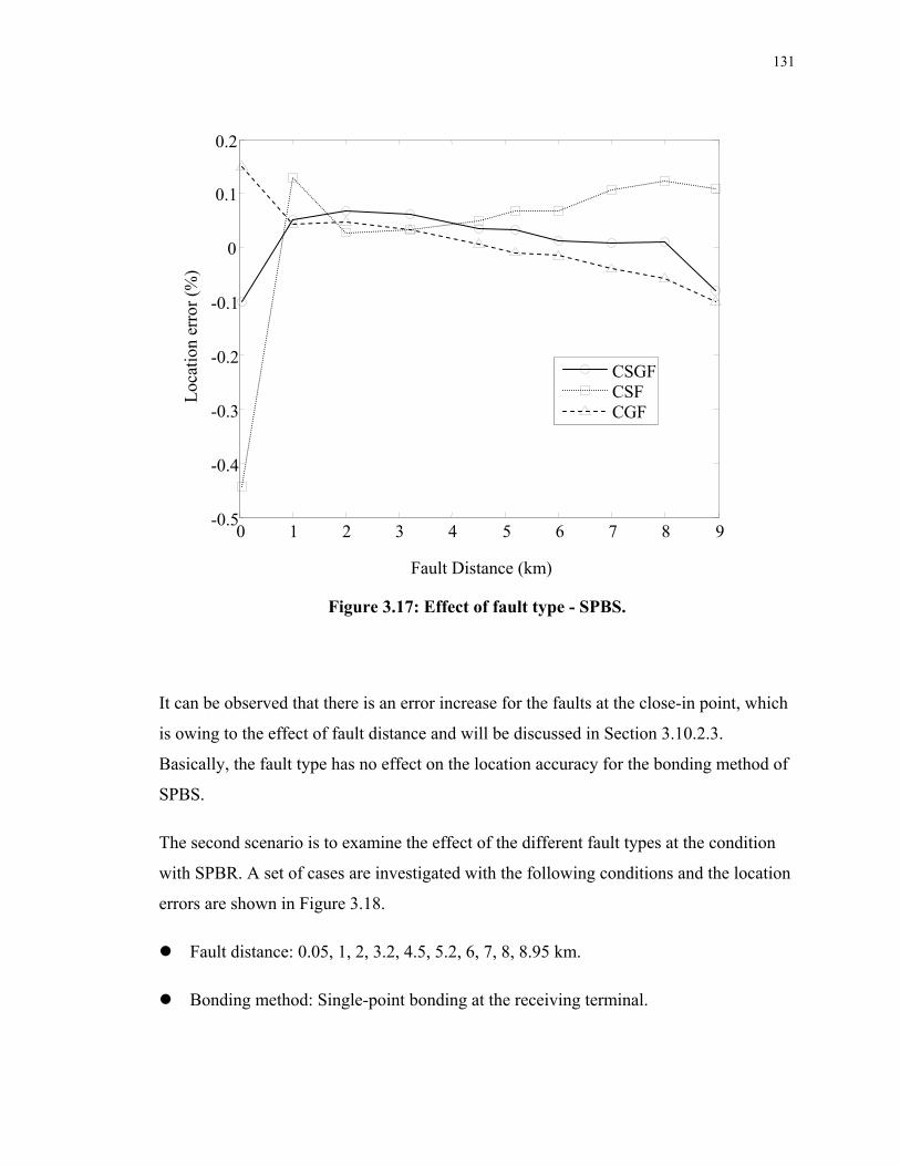
131
Figure 3.17: Effect of fault type - SPBS.
It can be observed that there is an error increase for the faults at the close-in point, which
is owing to the effect of fault distance and will be discussed in Section 3.10.2.3.
Basically, the fault type has no effect on the location accuracy for the bonding method of
SPBS.
The second scenario is to examine the effect of the different fault types at the condition
with SPBR. A set of cases are investigated with the following conditions and the location
errors are shown in Figure 3.18.
Fault distance: 0.05, 1, 2, 3.2, 4.5, 5.2, 6, 7, 8, 8.95 km.
Bonding method: Single-point bonding at the receiving terminal.
0 1 2 3 4 5 6 7 8 9-0.5
-0.4
-0.3
-0.2
-0.1
0
0.1
0.2
CSGF CSF CGF
Fault Distance (km)
Loc
atio
n er
ror
(%)
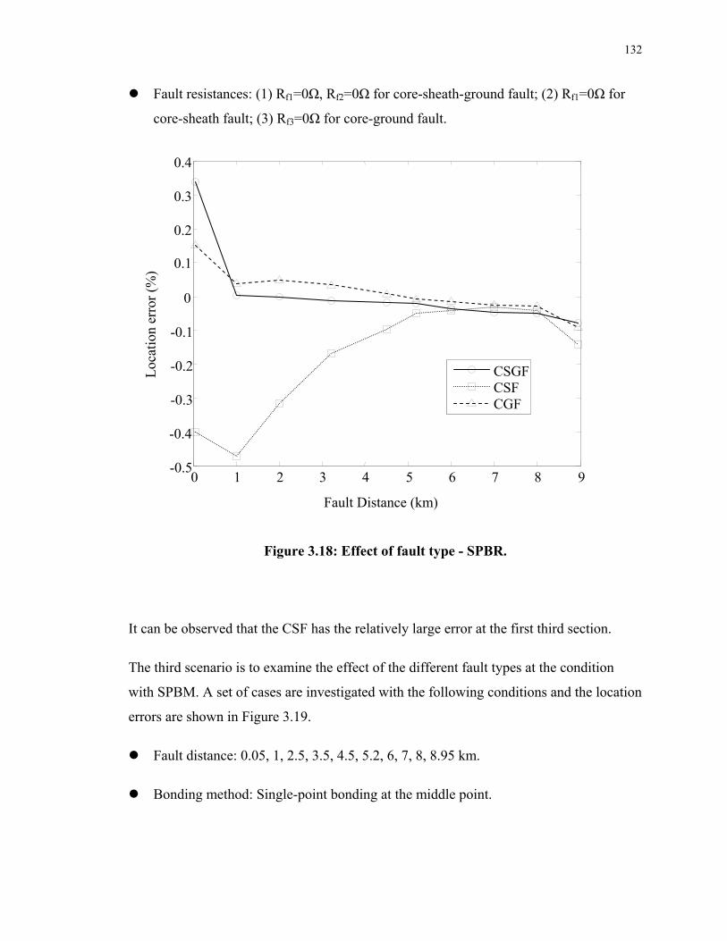
132
Fault resistances: (1) Rf1=0Ω, Rf2=0Ω for core-sheath-ground fault; (2) Rf1=0Ω for
core-sheath fault; (3) Rf3=0Ω for core-ground fault.
Figure 3.18: Effect of fault type - SPBR.
It can be observed that the CSF has the relatively large error at the first third section.
The third scenario is to examine the effect of the different fault types at the condition
with SPBM. A set of cases are investigated with the following conditions and the location
errors are shown in Figure 3.19.
Fault distance: 0.05, 1, 2.5, 3.5, 4.5, 5.2, 6, 7, 8, 8.95 km.
Bonding method: Single-point bonding at the middle point.
0 1 2 3 4 5 6 7 8 9-0.5
-0.4
-0.3
-0.2
-0.1
0
0.1
0.2
0.3
0.4
CSGF CSF CGF
Fault Distance (km)
Loc
atio
n er
ror
(%)
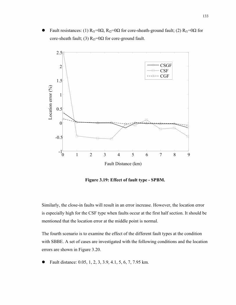
133
Fault resistances: (1) Rf1=0Ω, Rf2=0Ω for core-sheath-ground fault; (2) Rf1=0Ω for
core-sheath fault; (3) Rf3=0Ω for core-ground fault.
Figure 3.19: Effect of fault type - SPBM.
Similarly, the close-in faults will result in an error increase. However, the location error
is especially high for the CSF type when faults occur at the first half section. It should be
mentioned that the location error at the middle point is normal.
The fourth scenario is to examine the effect of the different fault types at the condition
with SBBE. A set of cases are investigated with the following conditions and the location
errors are shown in Figure 3.20.
Fault distance: 0.05, 1, 2, 3, 3.9, 4.1, 5, 6, 7, 7.95 km.
0 1 2 3 4 5 6 7 8 9-1
-0.5
0
0.5
1
1.5
2
2.5
CSGF CSF CGF
Fault Distance (km)
Loc
atio
n er
ror
(%)
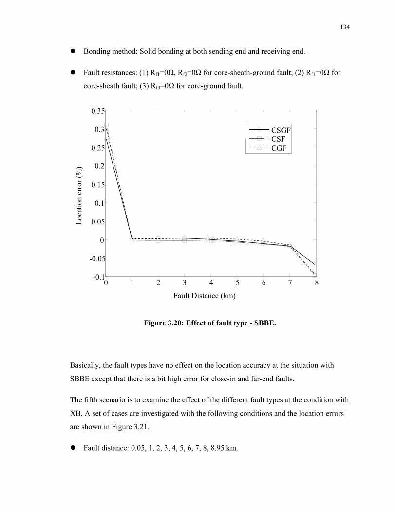
134
Bonding method: Solid bonding at both sending end and receiving end.
Fault resistances: (1) Rf1=0Ω, Rf2=0Ω for core-sheath-ground fault; (2) Rf1=0Ω for
core-sheath fault; (3) Rf3=0Ω for core-ground fault.
Figure 3.20: Effect of fault type - SBBE.
Basically, the fault types have no effect on the location accuracy at the situation with
SBBE except that there is a bit high error for close-in and far-end faults.
The fifth scenario is to examine the effect of the different fault types at the condition with
XB. A set of cases are investigated with the following conditions and the location errors
are shown in Figure 3.21.
Fault distance: 0.05, 1, 2, 3, 4, 5, 6, 7, 8, 8.95 km.
0 1 2 3 4 5 6 7 8-0.1
-0.05
0
0.05
0.1
0.15
0.2
0.25
0.3
0.35
Fault Distance (km)
CSGF CSF CGF
Loc
atio
n er
ror
(%)
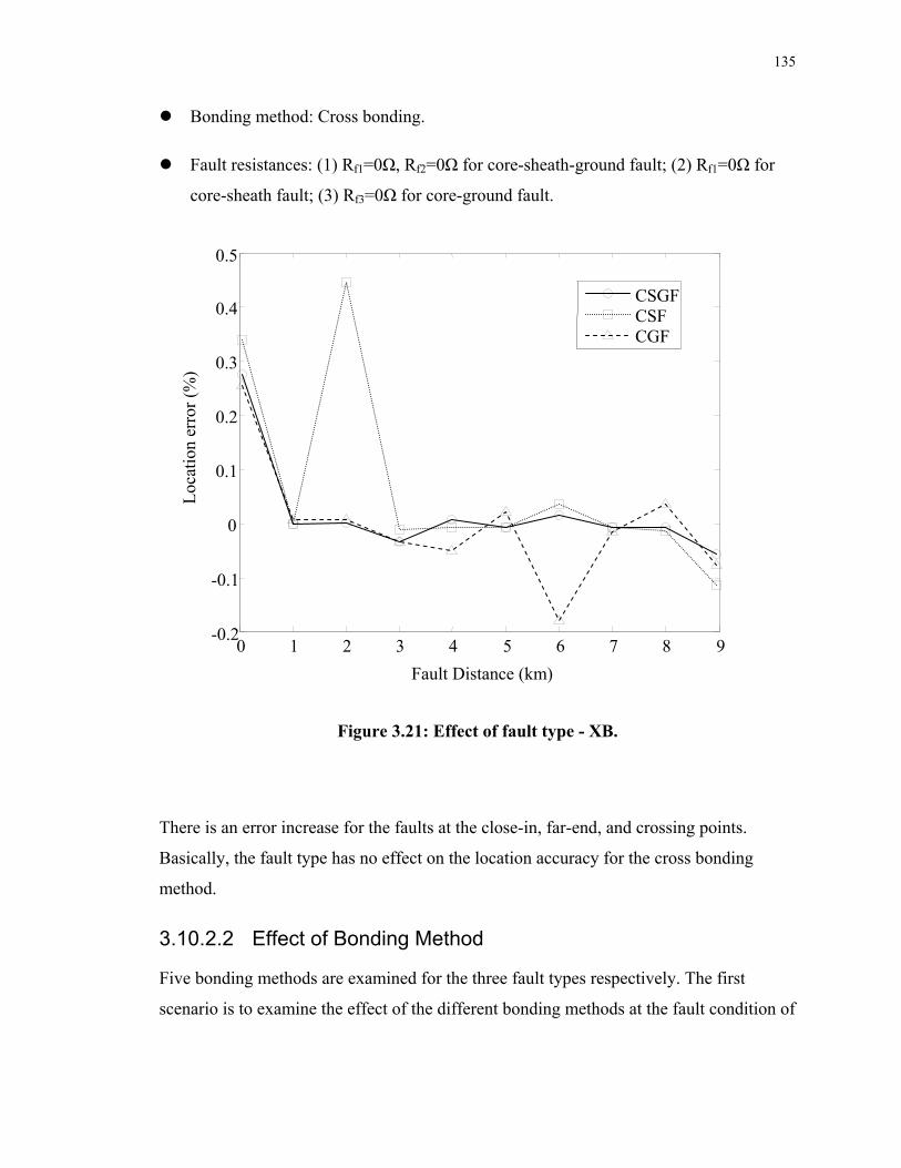
135
Bonding method: Cross bonding.
Fault resistances: (1) Rf1=0Ω, Rf2=0Ω for core-sheath-ground fault; (2) Rf1=0Ω for
core-sheath fault; (3) Rf3=0Ω for core-ground fault.
Figure 3.21: Effect of fault type - XB.
There is an error increase for the faults at the close-in, far-end, and crossing points.
Basically, the fault type has no effect on the location accuracy for the cross bonding
method.
3.10.2.2 Effect of Bonding Method
Five bonding methods are examined for the three fault types respectively. The first
scenario is to examine the effect of the different bonding methods at the fault condition of
0 1 2 3 4 5 6 7 8 9-0.2
-0.1
0
0.1
0.2
0.3
0.4
0.5
CSGF CSF CGF
Loc
atio
n er
ror
(%)
Fault Distance (km)
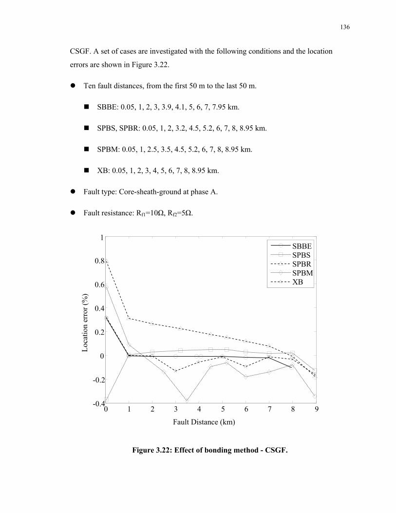
136
CSGF. A set of cases are investigated with the following conditions and the location
errors are shown in Figure 3.22.
Ten fault distances, from the first 50 m to the last 50 m.
SBBE: 0.05, 1, 2, 3, 3.9, 4.1, 5, 6, 7, 7.95 km.
SPBS, SPBR: 0.05, 1, 2, 3.2, 4.5, 5.2, 6, 7, 8, 8.95 km.
SPBM: 0.05, 1, 2.5, 3.5, 4.5, 5.2, 6, 7, 8, 8.95 km.
XB: 0.05, 1, 2, 3, 4, 5, 6, 7, 8, 8.95 km.
Fault type: Core-sheath-ground at phase A.
Fault resistance: Rf1=10Ω, Rf2=5Ω.
Figure 3.22: Effect of bonding method - CSGF.
0 1 2 3 4 5 6 7 8 9-0.4
-0.2
0
0.2
0.4
0.6
0.8
1
SBBE SPBS SPBR SPBM XB
Fault Distance (km)
Loc
atio
n er
ror
(%)
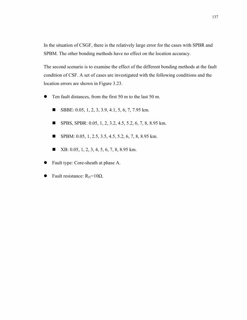
137
In the situation of CSGF, there is the relatively large error for the cases with SPBR and
SPBM. The other bonding methods have no effect on the location accuracy.
The second scenario is to examine the effect of the different bonding methods at the fault
condition of CSF. A set of cases are investigated with the following conditions and the
location errors are shown in Figure 3.23.
Ten fault distances, from the first 50 m to the last 50 m.
SBBE: 0.05, 1, 2, 3, 3.9, 4.1, 5, 6, 7, 7.95 km.
SPBS, SPBR: 0.05, 1, 2, 3.2, 4.5, 5.2, 6, 7, 8, 8.95 km.
SPBM: 0.05, 1, 2.5, 3.5, 4.5, 5.2, 6, 7, 8, 8.95 km.
XB: 0.05, 1, 2, 3, 4, 5, 6, 7, 8, 8.95 km.
Fault type: Core-sheath at phase A.
Fault resistance: Rf1=10Ω.
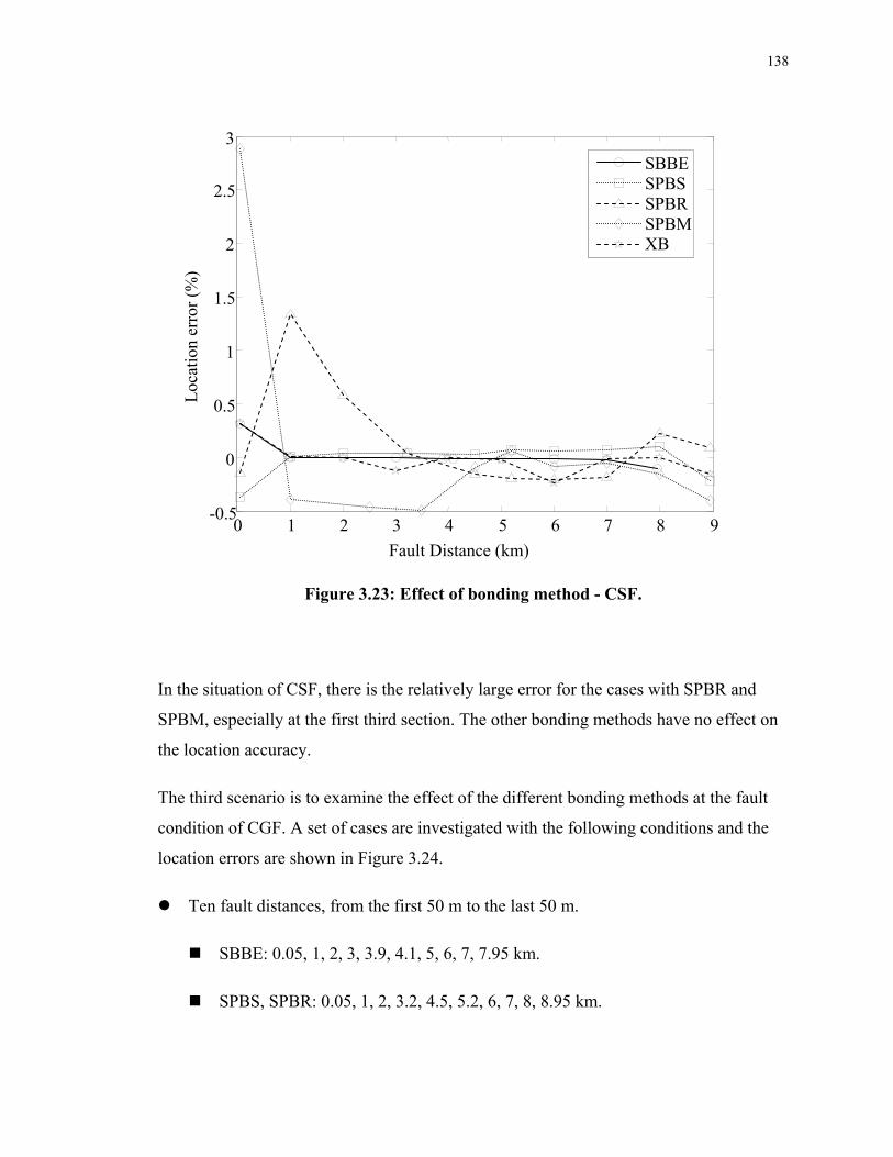
138
Figure 3.23: Effect of bonding method - CSF.
In the situation of CSF, there is the relatively large error for the cases with SPBR and
SPBM, especially at the first third section. The other bonding methods have no effect on
the location accuracy.
The third scenario is to examine the effect of the different bonding methods at the fault
condition of CGF. A set of cases are investigated with the following conditions and the
location errors are shown in Figure 3.24.
Ten fault distances, from the first 50 m to the last 50 m.
SBBE: 0.05, 1, 2, 3, 3.9, 4.1, 5, 6, 7, 7.95 km.
SPBS, SPBR: 0.05, 1, 2, 3.2, 4.5, 5.2, 6, 7, 8, 8.95 km.
0 1 2 3 4 5 6 7 8 9-0.5
0
0.5
1
1.5
2
2.5
3
SBBE SPBS SPBR SPBM XB
Fault Distance (km)
Loc
atio
n er
ror
(%)
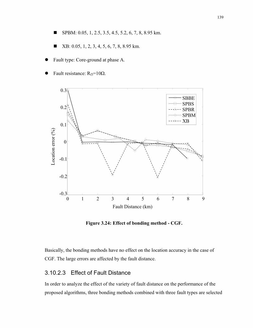
139
SPBM: 0.05, 1, 2.5, 3.5, 4.5, 5.2, 6, 7, 8, 8.95 km.
XB: 0.05, 1, 2, 3, 4, 5, 6, 7, 8, 8.95 km.
Fault type: Core-ground at phase A.
Fault resistance: Rf3=10Ω.
Figure 3.24: Effect of bonding method - CGF.
Basically, the bonding methods have no effect on the location accuracy in the case of
CGF. The large errors are affected by the fault distance.
3.10.2.3 Effect of Fault Distance
In order to analyze the effect of the variety of fault distance on the performance of the
proposed algorithms, three bonding methods combined with three fault types are selected
0 1 2 3 4 5 6 7 8 9-0.3
-0.2
-0.1
0
0.1
0.2
0.3
SBBE SPBS SPBR SPBM XB
Fault Distance (km)
Loc
atio
n er
ror
(%)
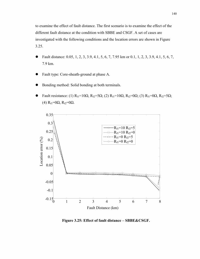
140
to examine the effect of fault distance. The first scenario is to examine the effect of the
different fault distance at the condition with SBBE and CSGF. A set of cases are
investigated with the following conditions and the location errors are shown in Figure
3.25.
Fault distance: 0.05, 1, 2, 3, 3.9, 4.1, 5, 6, 7, 7.95 km or 0.1, 1, 2, 3, 3.9, 4.1, 5, 6, 7,
7.9 km.
Fault type: Core-sheath-ground at phase A.
Bonding method: Solid bonding at both terminals.
Fault resistance: (1) Rf1=10Ω, Rf2=5Ω; (2) Rf1=10Ω, Rf2=0Ω; (3) Rf1=0Ω, Rf2=5Ω;
(4) Rf1=0Ω, Rf2=0Ω.
Figure 3.25: Effect of fault distance – SBBE&CSGF.
0 1 2 3 4 5 6 7 8-0.15
-0.1
-0.05
0
0.05
0.1
0.15
0.2
0.25
0.3
0.35
Rf1=10 Rf2=5 Rf1=10 Rf2=0 Rf1=0 Rf2=5 Rf1=0 Rf2=0
Fault Distance (km)
Loc
atio
n er
ror
(%)
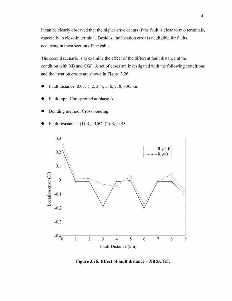
141
It can be clearly observed that the higher error occurs if the fault is close to two terminals,
especially to close-in terminal. Besides, the location error is negligible for faults
occurring in most section of the cable.
The second scenario is to examine the effect of the different fault distance at the
condition with XB and CGF. A set of cases are investigated with the following conditions
and the location errors are shown in Figure 3.26.
Fault distance: 0.05, 1, 2, 3, 4, 5, 6, 7, 8, 8.95 km.
Fault type: Core-ground at phase A.
Bonding method: Cross bonding.
Fault resistance: (1) Rf3=10Ω; (2) Rf3=0Ω.
Figure 3.26: Effect of fault distance – XB&CGF.
0 1 2 3 4 5 6 7 8 9-0.4
-0.3
-0.2
-0.1
0
0.1
0.2
0.3
Fault Distance (km)
Rf1=10 Rf1=0
Loc
atio
n er
ror
(%)
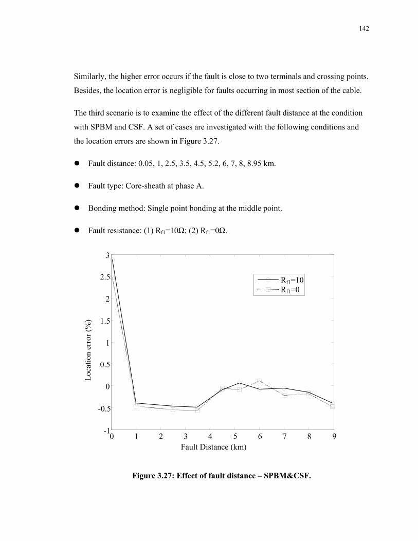
142
Similarly, the higher error occurs if the fault is close to two terminals and crossing points.
Besides, the location error is negligible for faults occurring in most section of the cable.
The third scenario is to examine the effect of the different fault distance at the condition
with SPBM and CSF. A set of cases are investigated with the following conditions and
the location errors are shown in Figure 3.27.
Fault distance: 0.05, 1, 2.5, 3.5, 4.5, 5.2, 6, 7, 8, 8.95 km.
Fault type: Core-sheath at phase A.
Bonding method: Single point bonding at the middle point.
Fault resistance: (1) Rf1=10Ω; (2) Rf1=0Ω.
Figure 3.27: Effect of fault distance – SPBM&CSF.
0 1 2 3 4 5 6 7 8 9-1
-0.5
0
0.5
1
1.5
2
2.5
3
Rf1=10 Rf1=0
Fault Distance (km)
Loc
atio
n er
ror
(%)
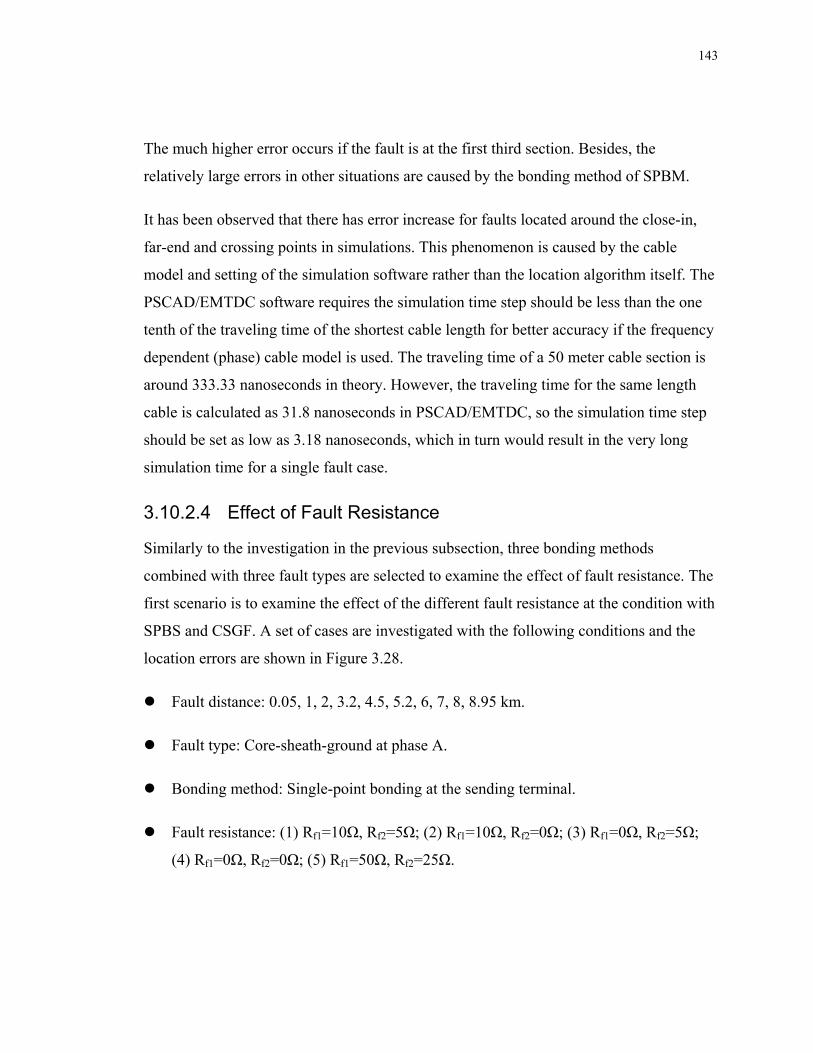
143
The much higher error occurs if the fault is at the first third section. Besides, the
relatively large errors in other situations are caused by the bonding method of SPBM.
It has been observed that there has error increase for faults located around the close-in,
far-end and crossing points in simulations. This phenomenon is caused by the cable
model and setting of the simulation software rather than the location algorithm itself. The
PSCAD/EMTDC software requires the simulation time step should be less than the one
tenth of the traveling time of the shortest cable length for better accuracy if the frequency
dependent (phase) cable model is used. The traveling time of a 50 meter cable section is
around 333.33 nanoseconds in theory. However, the traveling time for the same length
cable is calculated as 31.8 nanoseconds in PSCAD/EMTDC, so the simulation time step
should be set as low as 3.18 nanoseconds, which in turn would result in the very long
simulation time for a single fault case.
3.10.2.4 Effect of Fault Resistance
Similarly to the investigation in the previous subsection, three bonding methods
combined with three fault types are selected to examine the effect of fault resistance. The
first scenario is to examine the effect of the different fault resistance at the condition with
SPBS and CSGF. A set of cases are investigated with the following conditions and the
location errors are shown in Figure 3.28.
Fault distance: 0.05, 1, 2, 3.2, 4.5, 5.2, 6, 7, 8, 8.95 km.
Fault type: Core-sheath-ground at phase A.
Bonding method: Single-point bonding at the sending terminal.
Fault resistance: (1) Rf1=10Ω, Rf2=5Ω; (2) Rf1=10Ω, Rf2=0Ω; (3) Rf1=0Ω, Rf2=5Ω;
(4) Rf1=0Ω, Rf2=0Ω; (5) Rf1=50Ω, Rf2=25Ω.
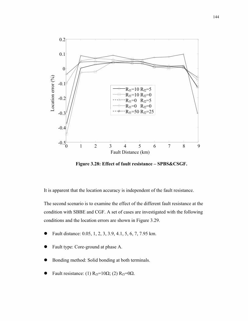
144
Figure 3.28: Effect of fault resistance – SPBS&CSGF.
It is apparent that the location accuracy is independent of the fault resistance.
The second scenario is to examine the effect of the different fault resistance at the
condition with SBBE and CGF. A set of cases are investigated with the following
conditions and the location errors are shown in Figure 3.29.
Fault distance: 0.05, 1, 2, 3, 3.9, 4.1, 5, 6, 7, 7.95 km.
Fault type: Core-ground at phase A.
Bonding method: Solid bonding at both terminals.
Fault resistance: (1) Rf3=10Ω; (2) Rf3=0Ω.
Rf1=10 Rf2=5 Rf1=10 Rf2=0 Rf1=0 Rf2=5 Rf1=0 Rf2=0 Rf1=50 Rf2=25
0 1 2 3 4 5 6 7 8 9-0.5
-0.4
-0.3
-0.2
-0.1
0
0.1
0.2
Fault Distance (km)
Loc
atio
n er
ror
(%)
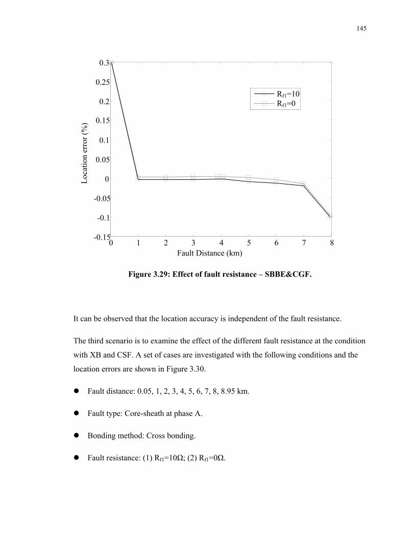
145
Figure 3.29: Effect of fault resistance – SBBE&CGF.
It can be observed that the location accuracy is independent of the fault resistance.
The third scenario is to examine the effect of the different fault resistance at the condition
with XB and CSF. A set of cases are investigated with the following conditions and the
location errors are shown in Figure 3.30.
Fault distance: 0.05, 1, 2, 3, 4, 5, 6, 7, 8, 8.95 km.
Fault type: Core-sheath at phase A.
Bonding method: Cross bonding.
Fault resistance: (1) Rf1=10Ω; (2) Rf1=0Ω.
0 1 2 3 4 5 6 7 8-0.15
-0.1
-0.05
0
0.05
0.1
0.15
0.2
0.25
0.3
Rf1=10 Rf1=0
Fault Distance (km)
Loc
atio
n er
ror
(%)
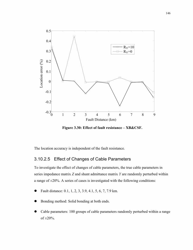
146
Figure 3.30: Effect of fault resistance – XB&CSF.
The location accuracy is independent of the fault resistance.
3.10.2.5 Effect of Changes of Cable Parameters
To investigate the effect of changes of cable parameters, the true cable parameters in
series impedance matrix Z and shunt admittance matrix Y are randomly perturbed within
a range of ±20%. A series of cases is investigated with the following conditions:
Fault distance: 0.1, 1, 2, 3, 3.9, 4.1, 5, 6, 7, 7.9 km.
Bonding method: Solid bonding at both ends.
Cable parameters: 100 groups of cable parameters randomly perturbed within a range
of ±20%.
0 1 2 3 4 5 6 7 8 9-0.3
-0.2
-0.1
0
0.1
0.2
0.3
0.4
0.5
Rf1=10 Rf1=0
Fault Distance (km)
Loc
atio
n er
ror
(%)
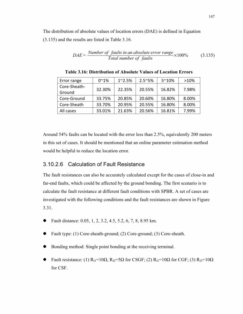
147
The distribution of absolute values of location errors (DAE) is defined in Equation
(3.135) and the results are listed in Table 3.16.
100%Number of faults in an absolute error range
DAE =Total number of faults
× (3.135)
Table 3.16: Distribution of Absolute Values of Location Errors
Error range 0~1% 1~2.5% 2.5~5% 5~10% >10% Core-Sheath- Ground 32.30% 22.35% 20.55% 16.82% 7.98%
Core-Ground 33.75% 20.85% 20.60% 16.80% 8.00% Core-Sheath 33.70% 20.95% 20.55% 16.80% 8.00% All cases 33.01% 21.63% 20.56% 16.81% 7.99%
Around 54% faults can be located with the error less than 2.5%, equivalently 200 meters
in this set of cases. It should be mentioned that an online parameter estimation method
would be helpful to reduce the location error.
3.10.2.6 Calculation of Fault Resistance
The fault resistances can also be accurately calculated except for the cases of close-in and
far-end faults, which could be affected by the ground bonding. The first scenario is to
calculate the fault resistance at different fault conditions with SPBR. A set of cases are
investigated with the following conditions and the fault resistances are shown in Figure
3.31.
Fault distance: 0.05, 1, 2, 3.2, 4.5, 5.2, 6, 7, 8, 8.95 km.
Fault type: (1) Core-sheath-ground; (2) Core-ground; (3) Core-sheath.
Bonding method: Single point bonding at the receiving terminal.
Fault resistance: (1) Rf1=10Ω, Rf2=5Ω for CSGF; (2) Rf1=10Ω for CGF; (3) Rf3=10Ω
for CSF.
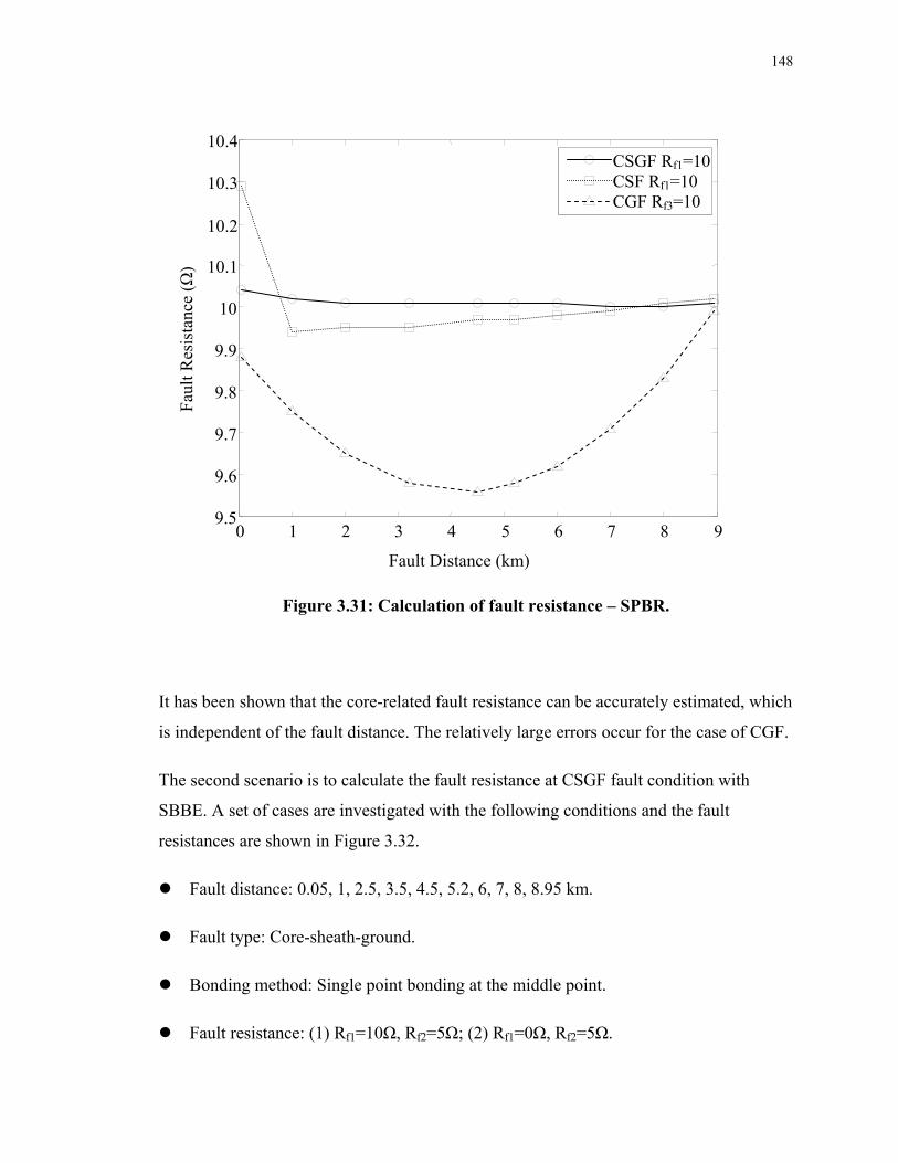
148
Figure 3.31: Calculation of fault resistance – SPBR.
It has been shown that the core-related fault resistance can be accurately estimated, which
is independent of the fault distance. The relatively large errors occur for the case of CGF.
The second scenario is to calculate the fault resistance at CSGF fault condition with
SBBE. A set of cases are investigated with the following conditions and the fault
resistances are shown in Figure 3.32.
Fault distance: 0.05, 1, 2.5, 3.5, 4.5, 5.2, 6, 7, 8, 8.95 km.
Fault type: Core-sheath-ground.
Bonding method: Single point bonding at the middle point.
Fault resistance: (1) Rf1=10Ω, Rf2=5Ω; (2) Rf1=0Ω, Rf2=5Ω.
0 1 2 3 4 5 6 7 8 99.5
9.6
9.7
9.8
9.9
10
10.1
10.2
10.3
10.4
CSGF Rf1=10 CSF Rf1=10 CGF Rf3=10
Fault Distance (km)
Fau
lt R
esis
tanc
e (Ω
)
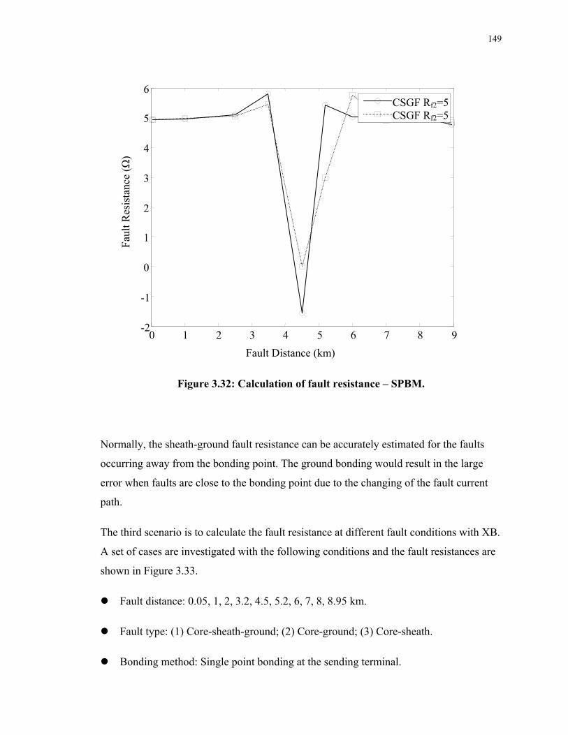
149
Figure 3.32: Calculation of fault resistance – SPBM.
Normally, the sheath-ground fault resistance can be accurately estimated for the faults
occurring away from the bonding point. The ground bonding would result in the large
error when faults are close to the bonding point due to the changing of the fault current
path.
The third scenario is to calculate the fault resistance at different fault conditions with XB.
A set of cases are investigated with the following conditions and the fault resistances are
shown in Figure 3.33.
Fault distance: 0.05, 1, 2, 3.2, 4.5, 5.2, 6, 7, 8, 8.95 km.
Fault type: (1) Core-sheath-ground; (2) Core-ground; (3) Core-sheath.
Bonding method: Single point bonding at the sending terminal.
0 1 2 3 4 5 6 7 8 9-2
-1
0
1
2
3
4
5
6
CSGF Rf2=5 CSGF Rf2=5
Fau
lt R
esis
tanc
e (Ω
)
Fault Distance (km)
150
Fault resistance: (1) Rf1=0Ω, Rf2=0Ω for CSGF; (2) Rf1=0Ω for CGF; (3) Rf3=0Ω for
CSF.
Figure 3.33: Calculation of fault resistance – SPBS.
The zero fault resistance can be accurately estimated in the cases of CSGF and CSF.
However, there has relatively large error in the case of CGF owing to the fact that the
fault resistance is not involved in the calculation of the CGF algorithm.
3.10.3 Summary of Effects
It has been tested that the fault resistance has no effect on the location accuracy.
Basically, the fault distance has no effect on the location accuracy, except that there has
an error increase for faults closed to the close-in, far-end and crossing points, which is
caused by the model and setting in the simulation software. The changes of cable
0 1 2 3 4 5 6 7 8 9-0.5
0
0.5
1
1.5
2
2.5
CSGF Rf1=0 CSF Rf1=0 CGF Rf3=0
Fault Distance (km)
Fau
lt R
esis
tanc
e (Ω
)

151
parameters would result in the large increase of the location error, but it can be averted by
an online parameter estimation method.
The effects of the bonding methods and fault types on the location accuracy are
summarized in Table 3.17.
Table 3.17: Effects of Bonding Methods and Fault Types on Location Accuracy
Core-Sheath- Ground Core-Ground Core-Sheath
Solid Bonding No effect No effect No effect Single Point @ Sending No effect No effect No effect
Single Point @ Receiving
Relatively large No effect Relatively large at
the first third section Single Point @ Middle
Relatively large No effect Relatively large at
the first half section Cross Bonding No effect No effect No effect
152
Chapter 4
4 Extension of the Proposed Fault Location Algorithms to Medium Voltage Cables in Distribution Networks
A set of the fault location algorithms for a plain cable with no laterals have been
presented in Chapter 3. The extensive simulations have validated the accuracy and
effectiveness of the proposed scheme. This chapter is to extend the proposed location
algorithms to underground distribution networks. In order to ensure the effectiveness of
location calculations, the voltages and currents at the sending terminal of the faulty cable
section, and the seen impedance behind the faulty section should be accurately estimated.
The power flow analysis or state estimation approach can provide the additional
information required by the location algorithm. Taking account of the complexity and
particularity of cable circuits in distribution networks, the state estimation for
underground distribution systems is formulated as a nonlinear optimization problem that
is solved by the sequential quadratic programming (SQP) technique. A section-by-section
estimation algorithm combined with the backward/forward sweep algorithm is proposed
to estimate the nodal voltage and branch current for each line section. The simulation
studies indicate the proposed fault location algorithm and the state estimation algorithm
can achieve good performance under different system and fault conditions.
The background knowledge is first introduced, including the complexities existing in
fault location calculations for cables, complexities existing in the state estimation for
distribution networks, problems emerging from the extension, and introduction to the
SQP nonlinear programming. Then the details of the proposed state estimation method
are discussed. A general location procedure combined with the proposed state estimation
technique is described as well. The application of the static response load model is
investigated. The algorithm is examined on a 31-node radial underground distribution
network, with consideration of laterals, tapped loads, unbalanced loads, different fault
types and fault distances.
153
4.1 Background
4.1.1 Complexities in Fault Location in Distribution Networks
The traditional fault analysis algorithms applied for transmission systems cannot
effectively achieve the expected performance in distribution systems due to the following
reasons.
Existence of short and heterogeneous feeders, including various size and length lines
and cables with different configurations.
Presence of laterals along the main feeder.
Presence of tapped loads distributed along the main feeder and laterals.
Unbalanced loads due to the presence of single phase, double-phase and three-phase
loads.
Untransposed lines and cables.
4.1.2 Complexities in State Estimation for Distribution Networks
Similarly, the traditional state estimation or power flow analysis algorithms applied for
transmission systems cannot be directly applied for distribution systems due to the
following facts [112].
Unbalanced system in nature, including laterals, tapped loads, and untransposed and
heterogeneous feeders.
Limited availability of real-time measurements.
Large number of loads.
For the sake of the accurate estimation, the state estimation for underground distribution
networks should consider the characteristics of cables, such as the relatively large
capacitance, effect of metallic sheath, sheath bonding method and unbalance impedance
matrix.
154
4.1.3 Emerging Issues Caused by Extension to Distribution Networks
It has been mentioned that the general logic principle in most of location algorithms is
first to determine the fault point in a plain line or cable with no laterals. Subsequently, the
location algorithm is extended to distribution networks taking account of the presence of
laterals, tapped loads, unbalanced loads, heterogeneity of lines, etc. The extension of such
a location algorithm for a plain line/cable into distribution networks causes three
technical issues.
How to obtain the voltage and current at the sending terminal of the faulty section?
How to estimate the seen load impedance at the receiving terminal of the faulty
section if the load impedance is required in calculations?
How to resolve the multiple estimates for possible faulty points due to the existence
of laterals? This problem specially exists in the impedance-based location
algorithms.
Due to the limited availability of measurements, the voltages and currents are usually
recorded at the substation in a distribution system. Therefore, the voltage and current can
be simply obtained by lumping all upstream loads and laterals between the substation and
faulty section, or gradually calculated node by node starting from the substation to the
faulty section. To carry out the above calculations, one prerequisite is the information of
laterals and tapped loads between the substation and faulty section should be available for
calculations. Similarly, the data of laterals and tapped loads behind the faulty section
should also be known to solve the second issue.
Overall, the load information prior to fault and during fault should be estimated for the
purpose of the accurate location. The sequential quadratic programming technique is
applied in this work to estimate the prefault voltage and load information of each node in
distribution networks.
155
4.1.4 Introduction to Sequential Quadratic Programming
Sequential quadratic programming (SQP) algorithms have proved to be fast and robust
for solving the general nonlinear optimization problem of the form [113],
,1, 2, ...,
( ) 0 1, 2, ...,
( ) 0 1, 2, ...,
Minimize f(x)subject to
l x u m nmCI x i piCE x j qj
≤ ≤ =≥ == =
(4.1)
where f(x), CI(x) and CE(x) are nonlinear smooth continuous functions which have
continuous second partial derivatives. The nonlinear problem has one quadratic objective
function f(x), n variables x, p inequality constraints CI(x), q equality constraints CE(x).
The notations l and u express the bound constraints on x.
The basic concept of SQP is to convert the nonlinear problem in Equation (4.1) into a
sequence of quadratic programming (QP) subproblems in Equation (4.2) where the
objective function is quadratic and the constraints are linear. Thus, SQP is converted to
an iterative method which solves a QP problem at each iteration.
,Minimize f(x)subject to
Ax bCx d
=≥
(4.2)
where f(x) is the quadratic objective function, and the matrices of A and C and the vectors
of b and d compose the linear constraints.
The solving procedure of SQP is available in many numerical optimization books such as
[113] and [114], free third party software, such as SQPlab [115], and commercial
mathematical tools, such as Matlab.
156
4.2 Development of State Estimation Algorithm
4.2.1 Problem Formulation
The state estimation for distribution networks can be used for different needs, such as
voltage monitoring and control at each bus, load control and service restoration for
individual loads, nodal pricing for aggregated loads, and fault location as suggested in
this work. Considering an underground distribution network, the known quantities and
preconditions can be summarized as follows.
Limited measurements, including three-phase voltages and three-phase currents of
the core conductors recorded at the substation, and other sparse measurements placed
in feeder transformers or important loads where voltage, current and/or power
quantities can be measured.
Load information can be acquired from the analysis of load forecast, documented in
the historical database, or analyzed from the load profiles.
Cable configuration and parameter would be stored in the database of utility
companies or obtained by other ways mentioned in Section 3.3.1. The information
includes the cable length, series impedance matrix, shunt admittance matrix and
sheath bonding method.
Owing to the availability of measurements and the uncertainty of load information, the
problem of the distribution state estimation can be formulated as a constrained nonlinear
optimization problem that incorporates the operating and loading constraints. The
voltages at each node are firstly estimated by solving the optimization problem, and
subsequently the loads are calculated based on the estimated voltages.
4.2.2 State Estimation Algorithm
The formulation of the state estimation is described as a constrained nonlinear
programming given as,
( ( )) 2Minimize W z f VV
− (4.3)
157
subject to,
min maxV V Vn n n≤ ≤ (4.4)
min maxn n nθ θ θ≤ ≤ (4.5)
est iniP Pn nPLB PUBn niniPn
−≤ ≤ (4.6)
est iniQ Qn nQLB QUB for each node nn niniQn
−≤ ≤ (4.7)
In the objective function (4.3), the voltage vector V is the set of state variables. The
vector z is the set of measurements. The function f(V) is the measurement function, where
the estimated measurements are calculated from the state variables. The matrix W is the
diagonal weighing matrix to rank different types of measurements with different
emphasis. The notation 2 denotes the Euclidean norm to evaluate the fitness of
weighted measurement residuals.
In the voltage constraints (4.4) and (4.5), the magnitude of the state variable V at each
node would be limited into a range from |V|min to |V|max. Similarly, the angle of the state
variable V at each node would be limited into a range from θmin to θmax.
In the loading constraints (4.6) and (4.7), the injected real power and reactive power Pest
and Qest at each node are estimated by f(V). The initial real power and reactive power at
each node Pini and Qini are obtained from the initial load information in advance. The
relative error between them should be in a range bounded by [PLB, PUB] and [QLB,
QUB].
4.2.2.1 Objective Function
The objective of the formulated optimization problem is to minimize the weighted errors
between the measurements (z) and the calculated results from the measurement function
158
(f(V)). Therefore, the estimated load flows can best fit measured load flows and adapt a
balance between the initial load information and calculated load outcome.
The measurement vector z denotes the measurements of the real power and reactive
power injected into each node, including the real-time measurements, zero-injection
measurements and load pseudo measurements. The real-time measurements are
physically sampled from sensors placed in networks sparsely. Since there have no enough
real-time measurements for the calculations of estimation, the load pseudo measurements
are introduced, which consider the known load information as a type of measurement
with less accuracy. The zero-injection measurements particularly represent the zero
injected power at the zero injection nodes and can also be regarded as the real-time
measurements or highly accurate pseudo measurements. There have twelve
measurements for a three-phase node, including three measurements of real part of real
power, three measurements of imaginary part of real power, three measurements of real
part of reactive power, and three measurements of imaginary part of reactive power.
Similarly, there have eight measurements for a two-phase node, and four for a single
phase node.
The measurement function f(V) is to calculate the injected power at each node based on
voltages at all adjacent nodes. For example, the injected power at node n can be
calculated as,
( )S S f Vn nk nkk An k An= =
∈ ∈ (4.8)
where Sn is the injected load flow at node n, Snk is the power flowing out of node n to
node k, and An is the set containing the nodes directly connected to node n. In the
example shown in Figure 4.1, An =m, s, t. The function fnk(V) is to calculate the branch
load flowing out of node n to node k based on the voltages at nodes n and k.
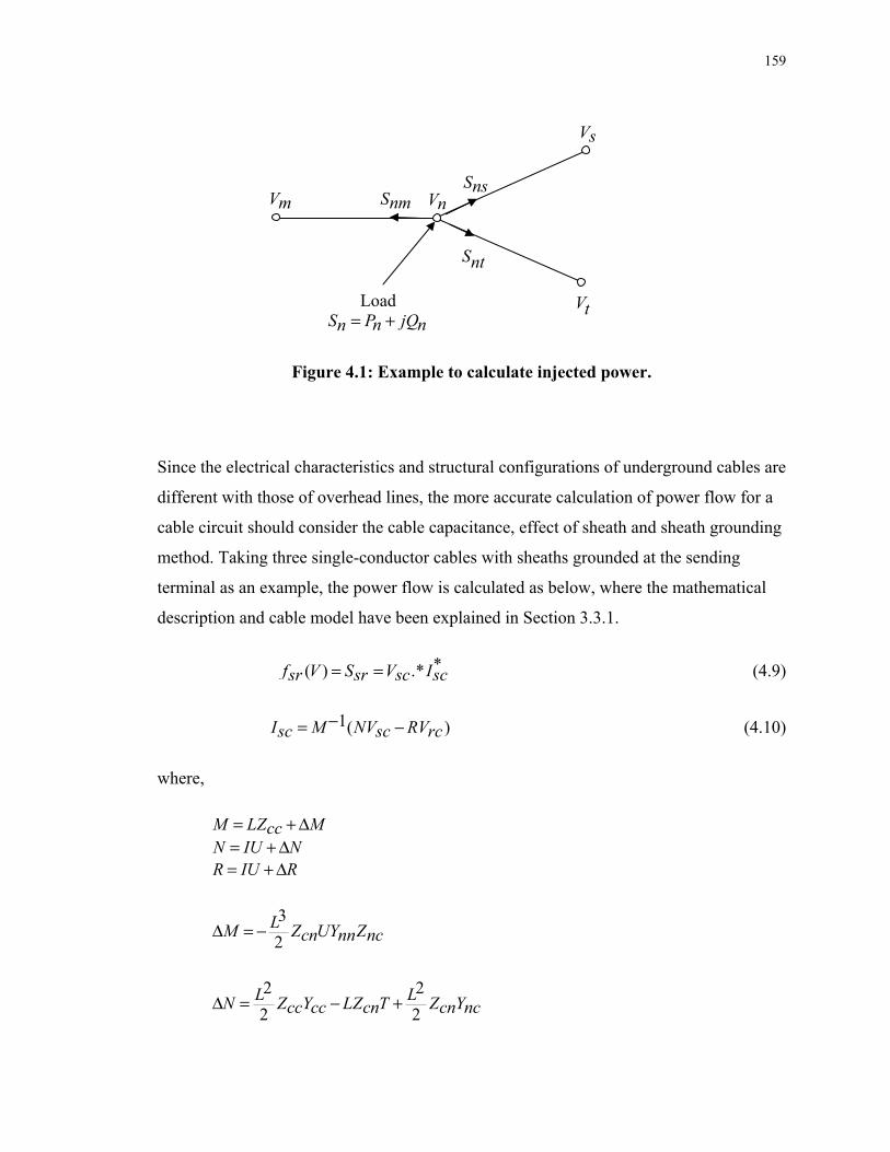
159
Figure 4.1: Example to calculate injected power.
Since the electrical characteristics and structural configurations of underground cables are
different with those of overhead lines, the more accurate calculation of power flow for a
cable circuit should consider the cable capacitance, effect of sheath and sheath grounding
method. Taking three single-conductor cables with sheaths grounded at the sending
terminal as an example, the power flow is calculated as below, where the mathematical
description and cable model have been explained in Section 3.3.1.
*( ) .*f V S V Isr sr sc sc= = (4.9)
1( )I M NV RVsc sc rc−= − (4.10)
where,
M LZ MccN IU NR IU R
= + Δ= + Δ= + Δ
3
2LM Z UY Zcn nn ncΔ = −
2 2
2 2L LN Z Y LZ T Z Ycc cc cn cn ncΔ = − +
Vm Vn
Vt
SnmSns
Snt
Load S P jQn nn = +
Vs
160
2
2LR Z UYcn ncΔ =
3 3( )2 4 4L L LT U Y Y Z Y Y Z Ync nn nc cc nn nn nc= + +
2 1( )2
LU IU Y Znn nn−= +
where V is the voltage phasor vector, I is the current phasor vector, Z is the series
impedance matrix, Y is the shunt admittance matrix, IU is the identity matrix, and L is the
length of cable. The symbol .* denotes the elementwise multiplication. The lowercase
subscript s means quantities at the sending terminal, similarly, r at the receiving terminal,
c for core conductor and n for sheath. Taking Zcn as an example, it indicates the mutual
impedance matrix per unit length between three cores and three sheaths, and so forth.
It is clear in Equation (4.10) that the power flow calculation for cables differs from the
classical equation for lines in the fact that there have three correction factors, ΔM, ΔN and
ΔR, which are caused by the particular characteristics and configurations of cables.
The matrix W in the objective function is the diagonal weighing matrix, which is
determined by the accuracy of corresponding measurements. For example, the real-time
measurements are most accurate and credible, so the largest weight values would be
assigned to the residuals of them. The notation 2 denotes the Euclidean norm, which is
defined as,
2 2 2...1 22x x x xn= + + + (4.11)
where the vector x=x1, x2, …, xn.
4.2.2.2 Voltage Constraints
The voltage at each node will maintain in a limited range around the nominal rating in the
normal operating condition. Therefore, this limited range can be used as the operating
constraints in Equations (4.4) and (4.5) to restrict the search region. Normally, this range
161
can be uniformly set within the ±3~5% of the voltages measured at the substation. The
values of real part and imaginary part can also be used as constraints rather than the
magnitude and angle. The state variables at each node contain six real variables for a
three-phase node, four for a two-phase node or two for a single phase node.
4.2.2.3 Loading Constraints
As mentioned in the above subsection, the known load information is considered as the
load pseudo measurements. However, this initial load information is obtained from the
load forecast, historical database or load profile, so it cannot accurately represent the true
load flow, which may be in a range around the initial load values. This range can be set as
the constraints in Equations (4.6) and (4.7) to further narrow down the search region,
which can also be expressed as,
.*est ini iniP P PB Pn n n n= + (4.12)
PLB PB PUBn n n≤ ≤ (4.13)
.*est ini iniQ Q QB Qn n n n= + (4.14)
QLB QB QUB for each node nn n n≤ ≤ (4.15)
where estPn and estQn express the injected real and reactive power calculated by
Equations (4.8)-(4.10), PBn and QBn are the load variation factors ranging from PLBn and
QLBn to PUBn and QUBn respectively.
Hitherto, the state estimation problem formulated in Equation (4.3) is in fact similar to
the general nonlinear optimization problem described in Equation (4.1), which can be
solved by the sequential quadratic programming methods.
4.3 General Location Procedure Combined with State Estimation
The general location procedure combined with the state estimation is described in this
section, which can be divided into four steps, i.e. prefault load estimation by DSE,
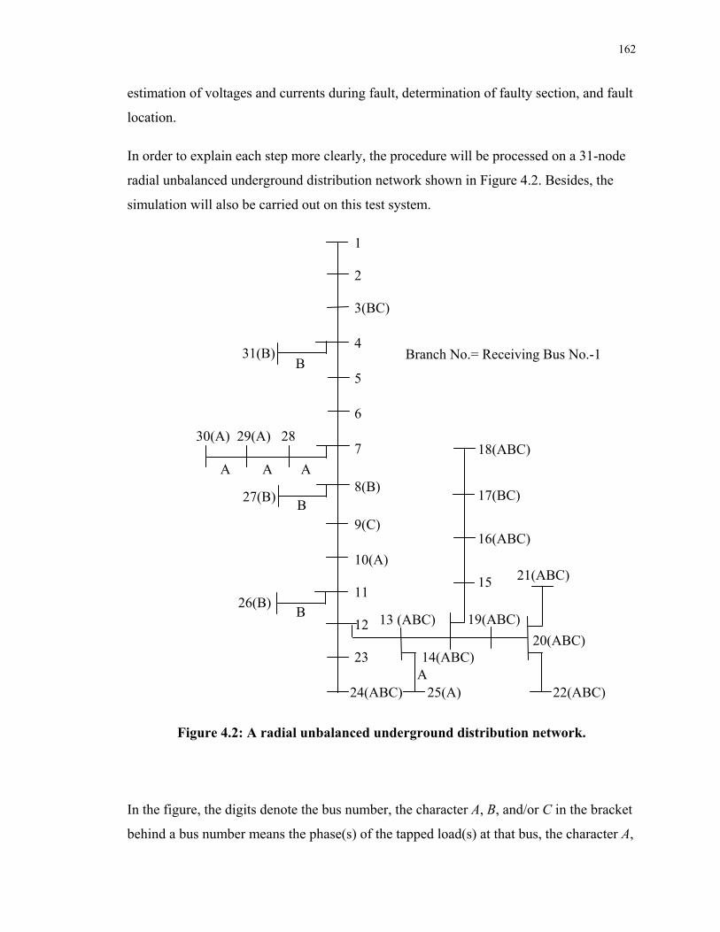
162
estimation of voltages and currents during fault, determination of faulty section, and fault
location.
In order to explain each step more clearly, the procedure will be processed on a 31-node
radial unbalanced underground distribution network shown in Figure 4.2. Besides, the
simulation will also be carried out on this test system.
Figure 4.2: A radial unbalanced underground distribution network.
In the figure, the digits denote the bus number, the character A, B, and/or C in the bracket
behind a bus number means the phase(s) of the tapped load(s) at that bus, the character A,
B31(B)
27(B)
A A A
30(A) 29(A) 28
13 (ABC)
B
B 26(B)
A
21(ABC)
14(ABC) 20(ABC)
18(ABC) 17(BC)
16(ABC)
15
24(ABC) 25(A) 22(ABC)
19(ABC)
1 2 3(BC) 4 5 6 7
8(B)
9(C) 10(A) 11 12 23
Branch No.= Receiving Bus No.-1
163
B, or C near a cable section expresses the phase of that lateral, and the section is a three-
phase feeder or lateral if there is no character near that section. The branch number is
equal to the receiving bus number minus one.
4.3.1 Prefault Load Estimation by DSE
The loads prior to the inception of a fault should be estimated in order to provide the real-
time load information for the fault location algorithm. This estimation process can be
regularly carried out in DMS, like every fifteen or thirty minutes. The results include the
estimated voltage at each node. Also the following quantities can be calculated by
Equations (4.8)-(4.10):
Branch current of each branch.
Branch real and reactive powers flowing in and out of a branch.
Injected load at each node.
Seen impedance behind each circuit section.
First, the initial load information can be acquired from the analysis of load forecast,
documented in the historical database, or analyzed from the load profiles. The initial
information can be used for two purposes:
Composing the pseudo measurements.
Calculating the voltage, Vprofile, at each node related to this specific load profile. The
applied algorithm is a section-by-section estimation algorithm combined with the
backward/forward sweep algorithm (BFSA) [58], which will be introduced in
Section 4.3.2.1.
Then, the state variables should be determined, including six real variables for each three-
phase node, four for each two-phase node or two for each single phase node. For example,
in the system in Figure 4.2, the total number of state variables is (24-1)×6+7×2=152. It
should be mentioned that the voltage at the substation bus is not counted as the state
variable.
164
Next, the initial values of state variables are calculated by scaling as below.
__ _ 0
_ 0
Vprofile iV Vinitial i initial Vprofile
= (4.16)
where Vprofile_i is the voltage at bus i estimated by the initial load profile. Vprofile_0 is the
voltage at the substation, which should be accurate for the corresponding load profile.
Vinitial_i is the initial voltage at bus i used for solving SE. Vinitial_0 is the voltage at the
substation, which is measured in real-time.
The voltage constraints are easily to be set. Normally, the constraint at each node can be
uniformly set within the ±3% of the Vinitial_i so that the voltage constraints can be
rewritten as,
0.97 1.03_ _V V Viinitial i initial i≤ ≤ (4.17)
0.97 1.03_ _V V Vinitial i i initial i∠ ≤ ∠ ≤ ∠ (4.18)
where Vi is the voltage at bus i, and is regarded as the state variable.
The initial loads are chosen to close to the true loads; however the real biases between
them are unknown. The loading constraints, PLBn, QLBn, PUBn and QUBn, can be
uniformly set as the constants. That is, the lower boundaries, PLBn and QLBn, are set to a
constant for all nodes, and the upper boundaries, PUBn and QUBn, are also set to a
constant for all nodes. The values of constants depend on the accuracy of the initial load
information. For example, if the initial load information is obtained from the load
forecast, which is supposed to be more accurate, the upper constant can be set to 0.05 and
the lower one to -0.05. And if the load is documented from a set of incomplete
information, the upper constant can be set to a value in the range from 0.05 to 0.2 and the
lower one could have the same value with the negative sign.
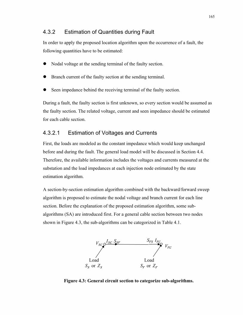
165
4.3.2 Estimation of Quantities during Fault
In order to apply the proposed location algorithm upon the occurrence of a fault, the
following quantities have to be estimated:
Nodal voltage at the sending terminal of the faulty section.
Branch current of the faulty section at the sending terminal.
Seen impedance behind the receiving terminal of the faulty section.
During a fault, the faulty section is first unknown, so every section would be assumed as
the faulty section. The related voltage, current and seen impedance should be estimated
for each cable section.
4.3.2.1 Estimation of Voltages and Currents
First, the loads are modeled as the constant impedance which would keep unchanged
before and during the fault. The general load model will be discussed in Section 4.4.
Therefore, the available information includes the voltages and currents measured at the
substation and the load impedances at each injection node estimated by the state
estimation algorithm.
A section-by-section estimation algorithm combined with the backward/forward sweep
algorithm is proposed to estimate the nodal voltage and branch current for each line
section. Before the explanation of the proposed estimation algorithm, some sub-
algorithms (SA) are introduced first. For a general cable section between two nodes
shown in Figure 4.3, the sub-algorithms can be categorized in Table 4.1.
Figure 4.3: General circuit section to categorize sub-algorithms.
Vsc Vrc
S Irs rc
Load Sr or Zr
Load Ss or Zs
I Ssc sr
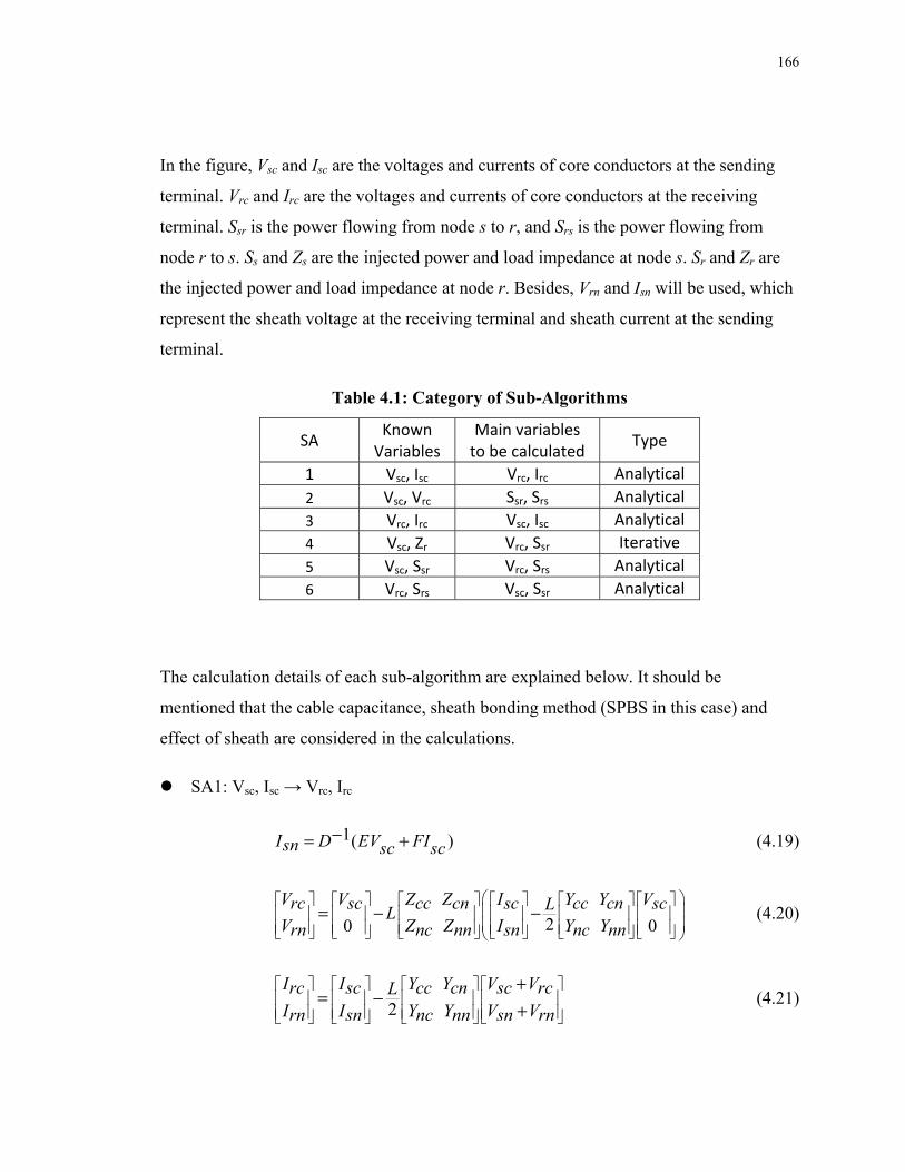
166
In the figure, Vsc and Isc are the voltages and currents of core conductors at the sending
terminal. Vrc and Irc are the voltages and currents of core conductors at the receiving
terminal. Ssr is the power flowing from node s to r, and Srs is the power flowing from
node r to s. Ss and Zs are the injected power and load impedance at node s. Sr and Zr are
the injected power and load impedance at node r. Besides, Vrn and Isn will be used, which
represent the sheath voltage at the receiving terminal and sheath current at the sending
terminal.
Table 4.1: Category of Sub-Algorithms
SA Known Variables
Main variables to be calculated Type
1 Vsc, Isc Vrc, Irc Analytical 2 Vsc, Vrc Ssr, Srs Analytical 3 Vrc, Irc Vsc, Isc Analytical 4 Vsc, Zr Vrc, Ssr Iterative 5 Vsc, Ssr Vrc, Srs Analytical 6 Vrc, Srs Vsc, Ssr Analytical
The calculation details of each sub-algorithm are explained below. It should be
mentioned that the cable capacitance, sheath bonding method (SPBS in this case) and
effect of sheath are considered in the calculations.
SA1: Vsc, Isc → Vrc, Irc
1( )I D EV FIsn sc sc−= + (4.19)
20 0
V Z Z I Y YV Vrc cc cn sc cc cnsc scLLV Z Z I Y Yrn nc nn sn nc nn
= − − (4.20)
2
I I Y Y V Vrc sc cc cn sc rcLI I Y Y V Vrn sn nc nn sn rn
+= −
+ (4.21)
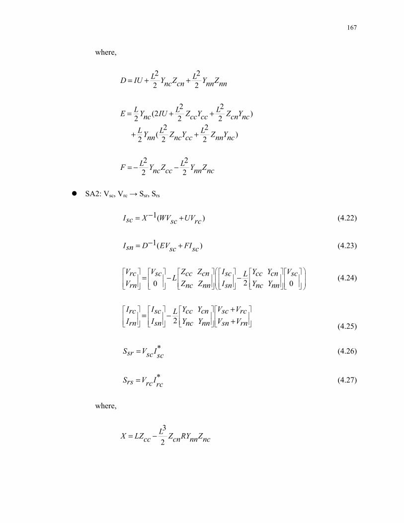
167
where,
2 2
2 2L LD IU Y Z Y Znc cn nn nn= + +
2 2(2 )
2 2 22 2
( )2 2 2
L L LE Y IU Z Y Z Ync cc cc cn nc
L L LY Z Y Z Ynn nc cc nn nc
= + +
+ +
2 2
2 2L LF Y Z Y Znc cc nn nc= − −
SA2: Vsc, Vrc → Ssr, Srs
1( )I X WV UVsc sc rc−= + (4.22)
1( )I D EV FIsn sc sc−= + (4.23)
20 0
V Z Z I Y YV Vrc cc cn sc cc cnsc scLLV Z Z I Y Yrn nc nn sn nc nn
= − − (4.24)
2
I I Y Y V Vrc sc cc cn sc rcLI I Y Y V Vrn sn nc nn sn rn
+= −
+ (4.25)
*S V Isr sc sc= (4.26)
*S V Irs rc rc= (4.27)
where,
3
2L
X LZ Z RY Zcc cn nn nc= −
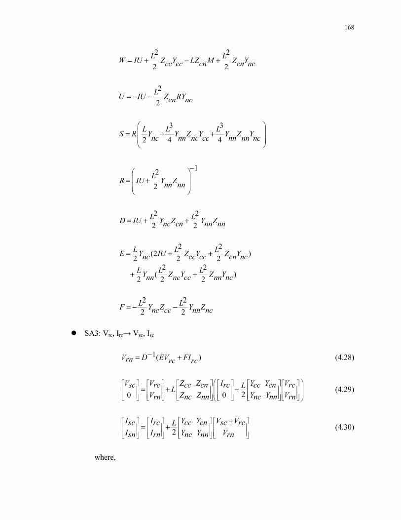
168
2 2
2 2L L
W IU Z Y LZ M Z Ycc cc cn cn nc= + − +
2
2L
U IU Z RYcn nc= − −
3 3
2 4 4L L L
S R Y Y Z Y Y Z Ync nn nc cc nn nn nc
= + +
12
2L
R IU Y Znn nn
− = +
2 2
2 2L LD IU Y Z Y Znc cn nn nn= + +
2 2(2 )
2 2 22 2
( )2 2 2
L L LE Y IU Z Y Z Ync cc cc cn nc
L L LY Z Y Z Ynn nc cc nn nc
= + +
+ +
2 2
2 2L LF Y Z Y Znc cc nn nc= − −
SA3: Vrc, Irc→ Vsc, Isc
1( )V D EV FIrn rc rc−= + (4.28)
20 0
V Z Z Y Y VV Irc cc cn cc cn rcsc rc LLV Z Z Y Y Vrn nc nn nc nn rn
= + + (4.29)
2
I I Y Y V Vsc rc cc cn sc rcLI I Y Y Vsn rn nc nn rn
+= + (4.30)
where,
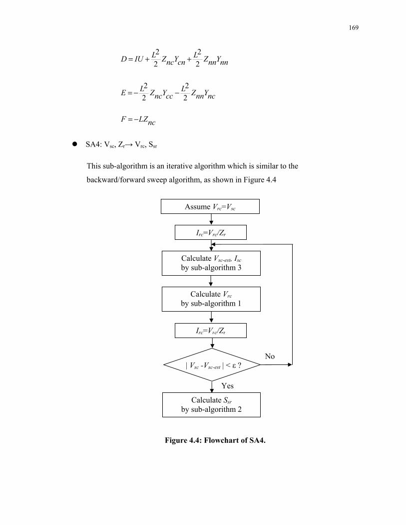
169
2 2
2 2L LD IU Z Y Z Ync cn nn nn= + +
2 2
2 2L LE Z Y Z Ync cc nn nc= − −
F LZnc= −
SA4: Vsc, Zr→ Vrc, Ssr
This sub-algorithm is an iterative algorithm which is similar to the
backward/forward sweep algorithm, as shown in Figure 4.4
Figure 4.4: Flowchart of SA4.
Assume Vrc=Vsc
| Vsc -Vsc-est | < ε ? No
Yes
Irc=Vrc/Zr
Calculate Vsc-est, Isc
by sub-algorithm 3
Calculate Vrc
by sub-algorithm 1
Irc=Vrc/Zr
Calculate Ssr
by sub-algorithm 2
170
SA5: Vsc, Ssr→ Vrc, Srs
*SsrIsc Vsc
=
(4.31)
1( )I D EV FIsn sc sc−= + (4.32)
20 0
V Z Z I Y YV Vrc cc cn sc cc cnsc scLLV Z Z I Y Yrn nc nn sn nc nn
= − − (4.33)
2
I I Y Y V Vrc sc cc cn sc rcLI I Y Y V Vrn sn nc nn sn rn
+= −
+ (4.34)
where,
2 2
2 2L LD IU Y Z Y Znc cn nn nn= + +
2 2(2 )
2 2 22 2
( )2 2 2
L L LE Y IU Z Y Z Ync cc cc cn nc
L L LY Z Y Z Ynn nc cc nn nc
= + +
+ +
2 2
2 2L LF Y Z Y Znc cc nn nc= − −
SA6: Vrc, Srs→ Vsc, Ssr
*SrsIrc Vrc
=
(4.35)
1( )V D EV FIrn rc rc−= + (4.36)
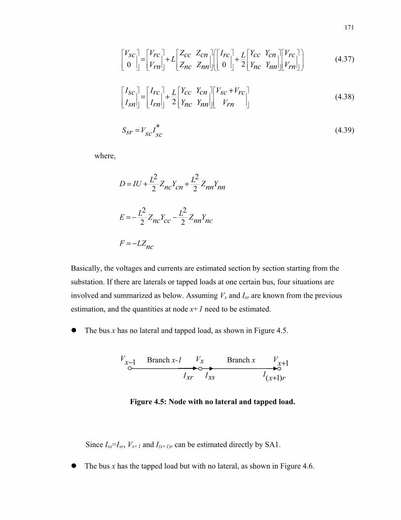
171
20 0
V Z Z Y Y VV Irc cc cn cc cn rcsc rc LLV Z Z Y Y Vrn nc nn nc nn rn
= + + (4.37)
2
I I Y Y V Vsc rc cc cn sc rcLI I Y Y Vsn rn nc nn rn
+= + (4.38)
*S V Isr sc sc= (4.39)
where,
2 2
2 2L LD IU Z Y Z Ync cn nn nn= + +
2 2
2 2L LE Z Y Z Ync cc nn nc= − −
F LZnc= −
Basically, the voltages and currents are estimated section by section starting from the
substation. If there are laterals or tapped loads at one certain bus, four situations are
involved and summarized as below. Assuming Vx and Ixr are known from the previous
estimation, and the quantities at node x+1 need to be estimated.
The bus x has no lateral and tapped load, as shown in Figure 4.5.
Figure 4.5: Node with no lateral and tapped load.
Since Ixs=Ixr, Vx+1 and I(x+1)r can be estimated directly by SA1.
The bus x has the tapped load but with no lateral, as shown in Figure 4.6.
1Vx− Branch x-1 Branch x
( 1)I x r+ Ixr
Vx 1Vx+
Ixs
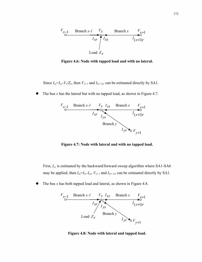
172
Figure 4.6: Node with tapped load and with no lateral.
Since Ixs=Ixr-Vx/Zx, then Vx+1 and I(x+1)r can be estimated directly by SA1.
The bus x has the lateral but with no tapped load, as shown in Figure 4.7.
Figure 4.7: Node with lateral and with no tapped load.
First, Iys is estimated by the backward/forward sweep algorithm where SA1-SA6
may be applied, then Ixs=Ixr-Iys, Vx+1 and I(x+1)r can be estimated directly by SA1.
The bus x has both tapped load and lateral, as shown in Figure 4.8.
Figure 4.8: Node with lateral and tapped load.
1Vx− Branch x-1 Branch x
( 1)I x r+ Ixr
Vx 1Vx+ Ixs
Branch y
I ys
I yrLoad Zx
1Vx− Branch x-1 Branch x
( 1)I x r+ Ixr
Vx 1Vx+ Ixs
Branch y
1Vy+
I ys
I yr
1Vx− Branch x-1 Branch x
( 1)I x r+ Ixr
Vx 1Vx+
Ixs
Load Zx
1Vy+
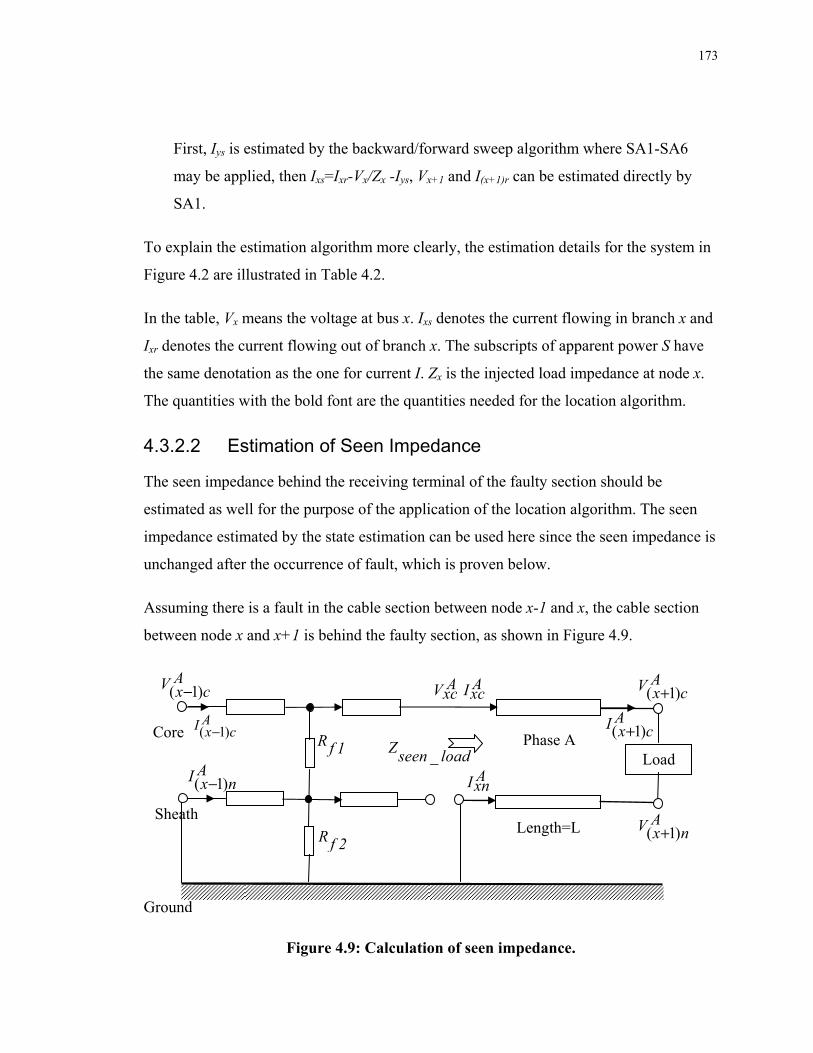
173
First, Iys is estimated by the backward/forward sweep algorithm where SA1-SA6
may be applied, then Ixs=Ixr-Vx/Zx -Iys, Vx+1 and I(x+1)r can be estimated directly by
SA1.
To explain the estimation algorithm more clearly, the estimation details for the system in
Figure 4.2 are illustrated in Table 4.2.
In the table, Vx means the voltage at bus x. Ixs denotes the current flowing in branch x and
Ixr denotes the current flowing out of branch x. The subscripts of apparent power S have
the same denotation as the one for current I. Zx is the injected load impedance at node x.
The quantities with the bold font are the quantities needed for the location algorithm.
4.3.2.2 Estimation of Seen Impedance
The seen impedance behind the receiving terminal of the faulty section should be
estimated as well for the purpose of the application of the location algorithm. The seen
impedance estimated by the state estimation can be used here since the seen impedance is
unchanged after the occurrence of fault, which is proven below.
Assuming there is a fault in the cable section between node x-1 and x, the cable section
between node x and x+1 is behind the faulty section, as shown in Figure 4.9.
Figure 4.9: Calculation of seen impedance.
Load Phase A
Length=L
( 1)AV x c+( 1)
AV x c−
( 1)AI x n−
( 1)AV x n+
R f 1
R f 2
A AV Ixc xc
AIxn
( 1)AI x c− ( 1)
AI x c+Core
Sheath
Ground
_Zseen load
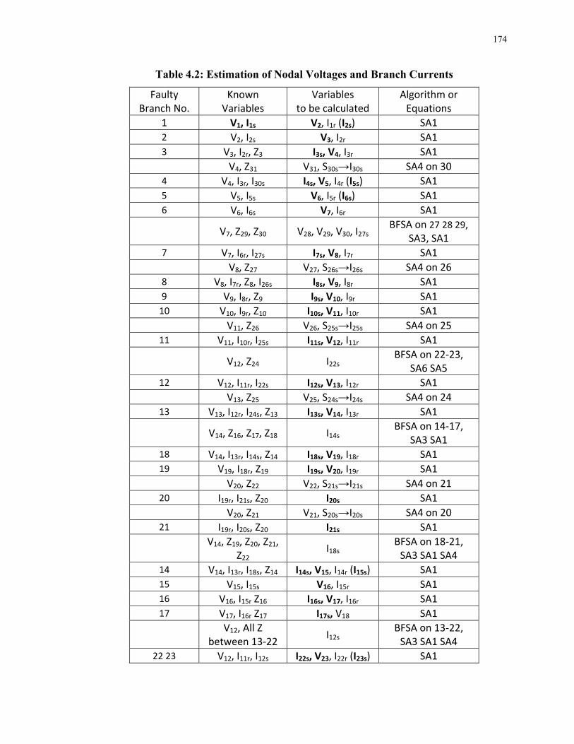
174
Table 4.2: Estimation of Nodal Voltages and Branch Currents
Faulty Branch No.
Known Variables
Variables to be calculated
Algorithm or Equations
1 V1, I1s V2, I1r (I2s) SA1 2 V2, I2s V3, I2r SA1 3 V3, I2r, Z3 I3s, V4, I3r SA1 V4, Z31 V31, S30s→I30s SA4 on 30
4 V4, I3r, I30s I4s, V5, I4r (I5s) SA1 5 V5, I5s V6, I5r (I6s) SA1 6 V6, I6s V7, I6r SA1
V7, Z29, Z30 V28, V29, V30, I27s BFSA on 27 28 29,
SA3, SA1 7 V7, I6r, I27s I7s, V8, I7r SA1 V8, Z27 V27, S26s→I26s SA4 on 26
8 V8, I7r, Z8, I26s I8s, V9, I8r SA1 9 V9, I8r, Z9 I9s, V10, I9r SA1
10 V10, I9r, Z10 I10s, V11, I10r SA1 V11, Z26 V26, S25s→I25s SA4 on 25
11 V11, I10r, I25s I11s, V12, I11r SA1
V12, Z24 I22s BFSA on 22-23,
SA6 SA5 12 V12, I11r, I22s I12s, V13, I12r SA1
V13, Z25 V25, S24s→I24s SA4 on 24 13 V13, I12r, I24s, Z13 I13s, V14, I13r SA1
V14, Z16, Z17, Z18 I14s BFSA on 14-17,
SA3 SA1 18 V14, I13r, I14s, Z14 I18s, V19, I18r SA1 19 V19, I18r, Z19 I19s, V20, I19r SA1
V20, Z22 V22, S21s→I21s SA4 on 21 20 I19r, I21s, Z20 I20s SA1
V20, Z21 V21, S20s→I20s SA4 on 20 21 I19r, I20s, Z20 I21s SA1
V14, Z19, Z20, Z21, Z22 I18s
BFSA on 18-21, SA3 SA1 SA4
14 V14, I13r, I18s, Z14 I14s, V15, I14r (I15s) SA1 15 V15, I15s V16, I15r SA1 16 V16, I15r Z16 I16s, V17, I16r SA1 17 V17, I16r Z17 I17s, V18 SA1
V12, All Z between 13-22 I12s
BFSA on 13-22, SA3 SA1 SA4
22 23 V12, I11r, I12s I22s, V23, I22r (I23s) SA1
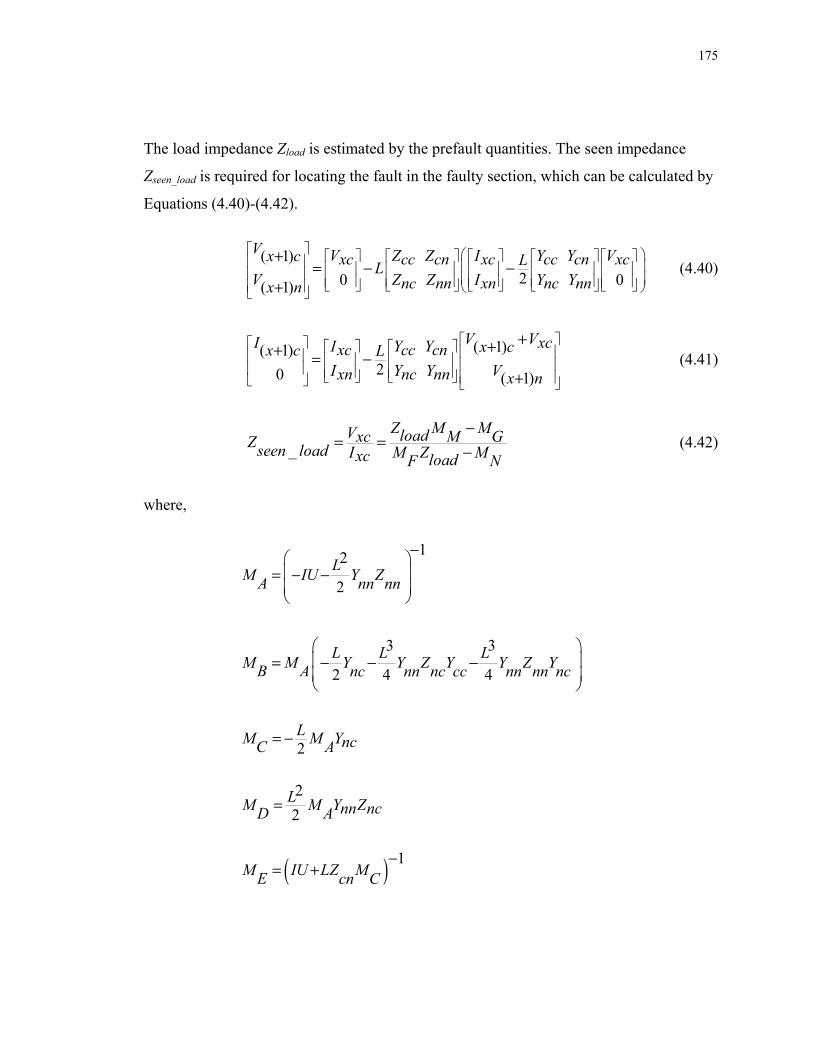
175
The load impedance Zload is estimated by the prefault quantities. The seen impedance
Zseen_load is required for locating the fault in the faulty section, which can be calculated by
Equations (4.40)-(4.42).
( 1)
20 0( 1)
V Z Z I Y YV Vx c cc cn xc cc cnxc xcLLV Z Z I Y Ync nn xn nc nnx n
+= − −
+ (4.40)
( 1)( 1)20 ( 1)
V VxcI I Y Y x cxc cc cnx c LI Y Y Vxn nc nn x n
+++ = −+
(4.41)
_
Z M MV loadxc M GZseen load I M Z Mxc loadF N
−= = − (4.42)
where,
12
2L
M IU Y ZA nn nn
− = − −
3 3
2 4 4L L L
M M Y Y Z Y Y Z YB A nc nn nc cc nn nn nc
= − − −
2LM M YncC A= −
2
2LM M Y Znn ncD A=
( ) 1M IU LZ ME cn C
−= +
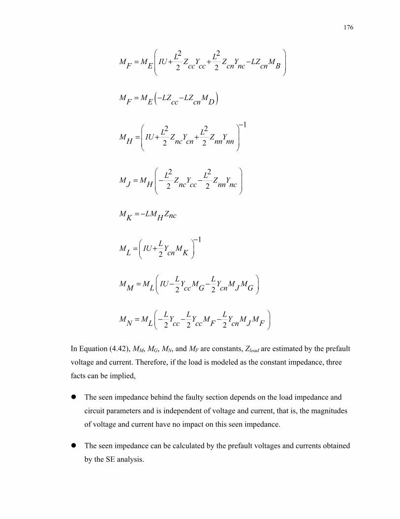
176
2 2
2 2L L
M M IU Z Y Z Y LZ MF E cc cc cn nc cn B
= + + −
( )M M LZ LZ MF E cc cn D= − −
12 2
2 2L L
M IU Z Y Z YH nc cn nn nn
− = + +
2 2
2 2L L
M M Z Y Z YJ H nc cc nn nc
= − −
M LM ZncK H= −
1
2L
M IU Y ML cn K
− = +
2 2L L
M M IU Y M Y M MM L cc G cn J G = − −
2 2 2L L L
M M Y Y M Y M MN L cc cc F cn J F = − − −
In Equation (4.42), MM, MG, MN, and MF are constants, Zload are estimated by the prefault
voltage and current. Therefore, if the load is modeled as the constant impedance, three
facts can be implied,
The seen impedance behind the faulty section depends on the load impedance and
circuit parameters and is independent of voltage and current, that is, the magnitudes
of voltage and current have no impact on this seen impedance.
The seen impedance can be calculated by the prefault voltages and currents obtained
by the SE analysis.

177
All downstream feeders, laterals and loads behind the faulty section can be lumped
as the seen impedance by this way.
4.3.3 Determination of Faulty Section
So far, the voltage and current at the sending terminal of each section, and the seen
impedance behind each section have been estimated. The proposed location algorithm
can be applied for each cable section, starting from the source.
If the location calculation is processed on a healthy cable, one or more of the following
phenomena could be observed:
No line-circle crossing point when estimating the current of the faulty sheath;
Multiple zigzags in the curves of the pinpoint criteria;
Singular matrix in the process of calculations.
Therefore, the true faulty section is identified as the section with the definite line-circle
crossing points, smooth curves of the pinpoint criteria, and well-conditioned matrix in
calculation.
Based on the test system in Figure 4.2, three examples with CSGF are given to show the
process of determination of the faulty section.
The first example shows a fault occurs at the branch 1 between node 1 and 2. As
illustrated in Figure 4.10, there exists the line crossing circle zone along the cable, the
pinpoint criteria are smooth, and the minimal point can be clearly found in the curve of
the pinpoint criterion. However, these phenomena cannot be observed in Figure 4.11
where the location calculation is processed in the healthy branch 2. Other healthy
branches have the similar problem. Therefore, the faulty section can be identified as the
branch 1.
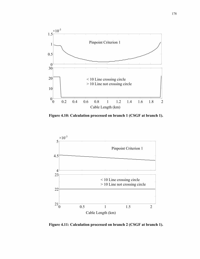
178
Figure 4.10: Calculation processed on branch 1 (CSGF at branch 1).
Figure 4.11: Calculation processed on branch 2 (CSGF at branch 1).
0
0.5
1
1.5
0 0.2 0.4 0.6 0.8 1 1.2 1.4 1.6 1.8 20
10
20
30
Pinpoint Criterion 1
< 10 Line crossing circle > 10 Line not crossing circle
×10-3
Cable Length (km)
4
4.5
5
0 0.5 1 1.5 2 21
22
23 < 10 Line crossing circle > 10 Line not crossing circle
Pinpoint Criterion 1
×10-3
Cable Length (km)
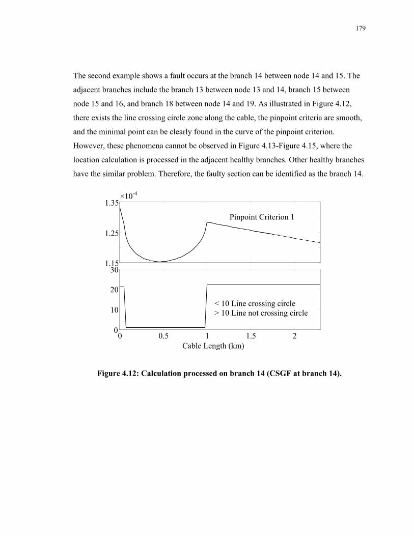
179
The second example shows a fault occurs at the branch 14 between node 14 and 15. The
adjacent branches include the branch 13 between node 13 and 14, branch 15 between
node 15 and 16, and branch 18 between node 14 and 19. As illustrated in Figure 4.12,
there exists the line crossing circle zone along the cable, the pinpoint criteria are smooth,
and the minimal point can be clearly found in the curve of the pinpoint criterion.
However, these phenomena cannot be observed in Figure 4.13-Figure 4.15, where the
location calculation is processed in the adjacent healthy branches. Other healthy branches
have the similar problem. Therefore, the faulty section can be identified as the branch 14.
Figure 4.12: Calculation processed on branch 14 (CSGF at branch 14).
1.15
1.25
1.35
0 0.5 1 1.5 2 0
10
20
30
Pinpoint Criterion 1
< 10 Line crossing circle > 10 Line not crossing circle
×10-4
Cable Length (km)
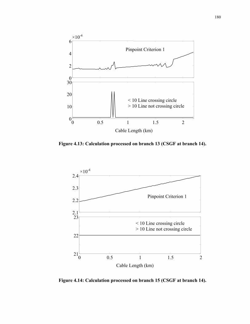
180
Figure 4.13: Calculation processed on branch 13 (CSGF at branch 14).
Figure 4.14: Calculation processed on branch 15 (CSGF at branch 14).
0
2
4
6
0 0.5 1 1.5 2 0
10
20
30
< 10 Line crossing circle > 10 Line not crossing circle
Pinpoint Criterion 1
×10-4
Cable Length (km)
2.1
2.2
2.3
2.4
0 0.5 1 1.5 221
22
23 < 10 Line crossing circle > 10 Line not crossing circle
Pinpoint Criterion 1
Cable Length (km)
×10-4
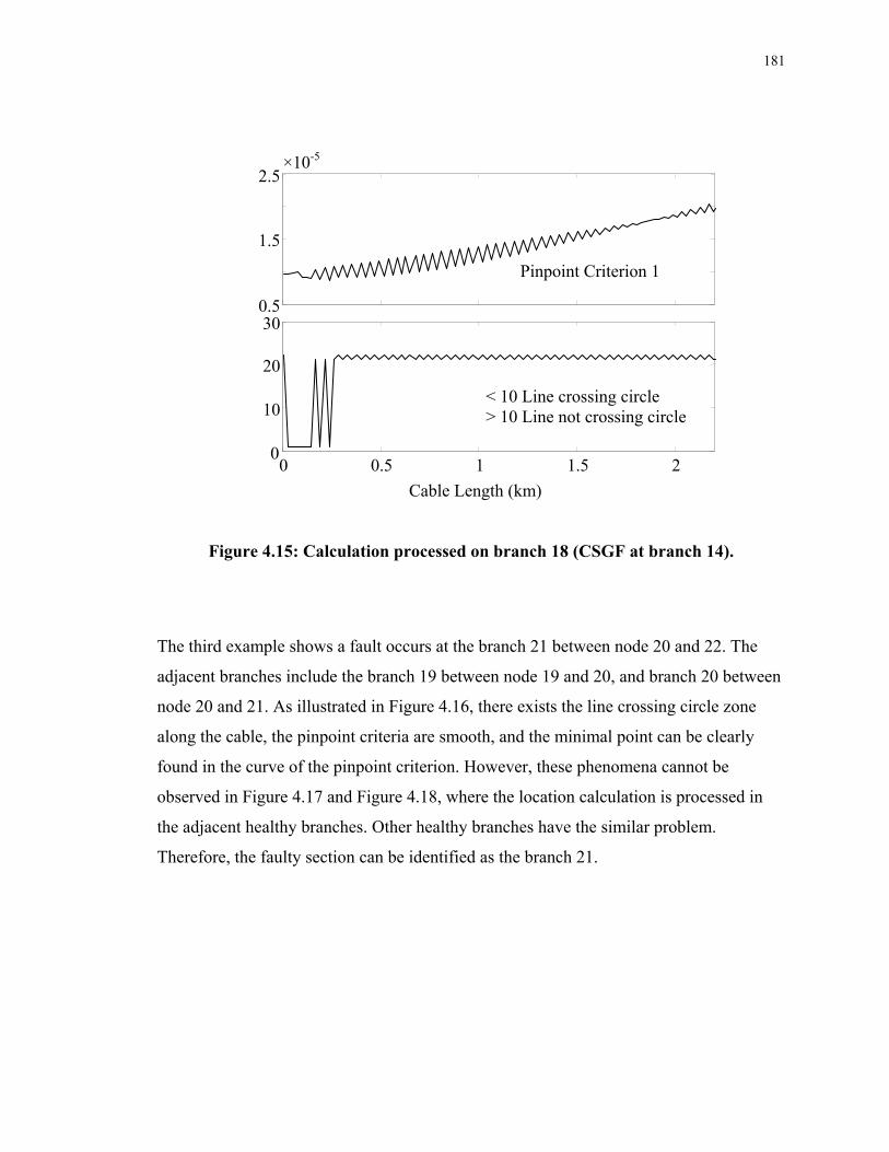
181
Figure 4.15: Calculation processed on branch 18 (CSGF at branch 14).
The third example shows a fault occurs at the branch 21 between node 20 and 22. The
adjacent branches include the branch 19 between node 19 and 20, and branch 20 between
node 20 and 21. As illustrated in Figure 4.16, there exists the line crossing circle zone
along the cable, the pinpoint criteria are smooth, and the minimal point can be clearly
found in the curve of the pinpoint criterion. However, these phenomena cannot be
observed in Figure 4.17 and Figure 4.18, where the location calculation is processed in
the adjacent healthy branches. Other healthy branches have the similar problem.
Therefore, the faulty section can be identified as the branch 21.
0.5
1.5
2.5
0 0.5 1 1.5 2 0
10
20
30
< 10 Line crossing circle > 10 Line not crossing circle
Pinpoint Criterion 1
Cable Length (km)
×10-5
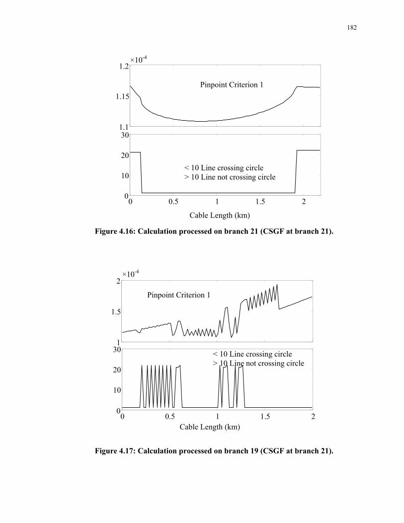
182
Figure 4.16: Calculation processed on branch 21 (CSGF at branch 21).
Figure 4.17: Calculation processed on branch 19 (CSGF at branch 21).
1
1.5
2
0 0.5 1 1.5 2 0
10
20
30
Pinpoint Criterion 1
< 10 Line crossing circle > 10 Line not crossing circle
×10-4
Cable Length (km)
1.1
1.15
1.2
0 0.5 1 1.5 2 0
10
20
30
< 10 Line crossing circle > 10 Line not crossing circle
Pinpoint Criterion 1
×10-4
Cable Length (km)
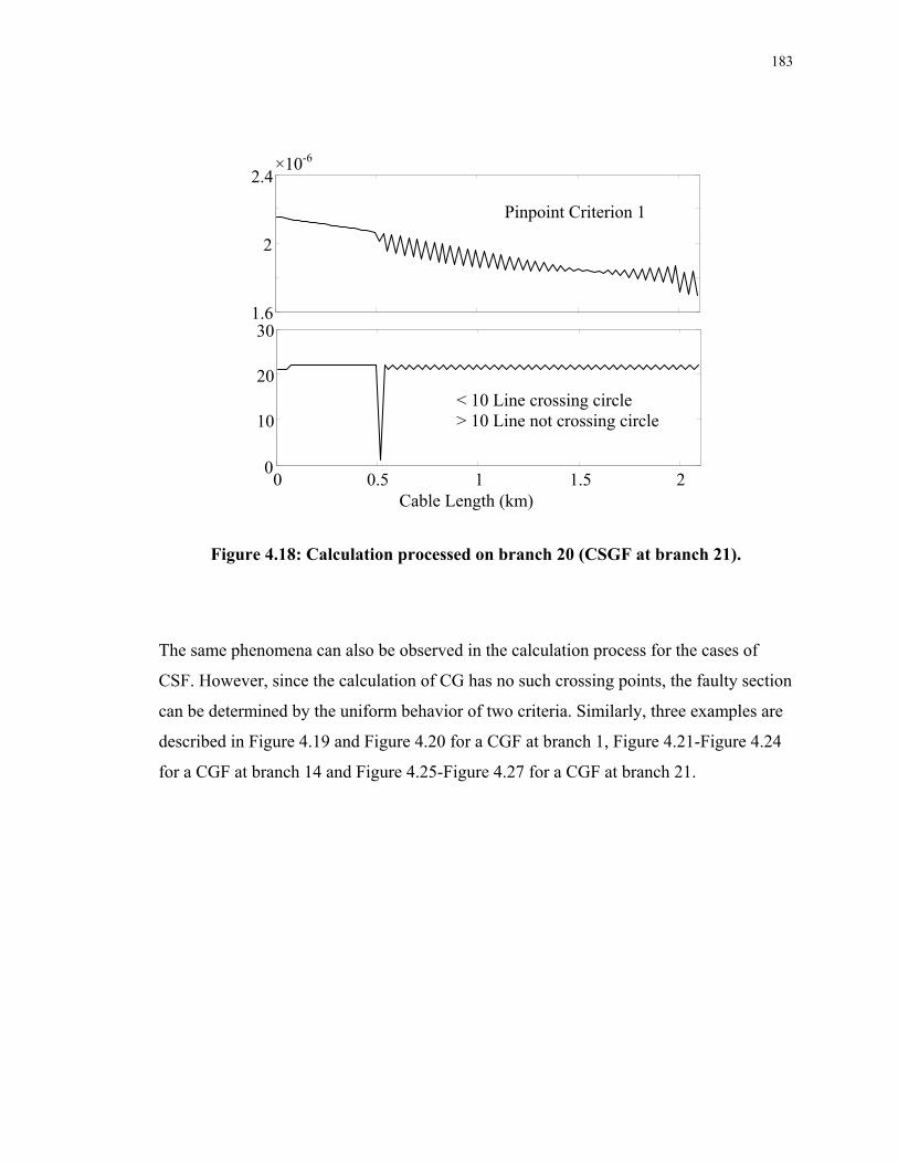
183
Figure 4.18: Calculation processed on branch 20 (CSGF at branch 21).
The same phenomena can also be observed in the calculation process for the cases of
CSF. However, since the calculation of CG has no such crossing points, the faulty section
can be determined by the uniform behavior of two criteria. Similarly, three examples are
described in Figure 4.19 and Figure 4.20 for a CGF at branch 1, Figure 4.21-Figure 4.24
for a CGF at branch 14 and Figure 4.25-Figure 4.27 for a CGF at branch 21.
1.6
2
2.4
0 0.5 1 1.5 2 0
10
20
30
Pinpoint Criterion 1
< 10 Line crossing circle > 10 Line not crossing circle
×10-6
Cable Length (km)
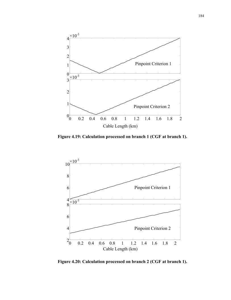
184
Figure 4.19: Calculation processed on branch 1 (CGF at branch 1).
Figure 4.20: Calculation processed on branch 2 (CGF at branch 1).
0
1
2
3
4
0 0.2 0.4 0.6 0.8 1 1.2 1.4 1.6 1.8 2 0
1
2
3
×10-3
×10-3
Pinpoint Criterion 1
Pinpoint Criterion 2
Cable Length (km)
4
6
8
10
0 0.2 0.4 0.6 0.8 1 1.2 1.4 1.6 1.8 2 2
4
6
8
×10-3
×10-3
Cable Length (km)
Pinpoint Criterion 2
Pinpoint Criterion 1
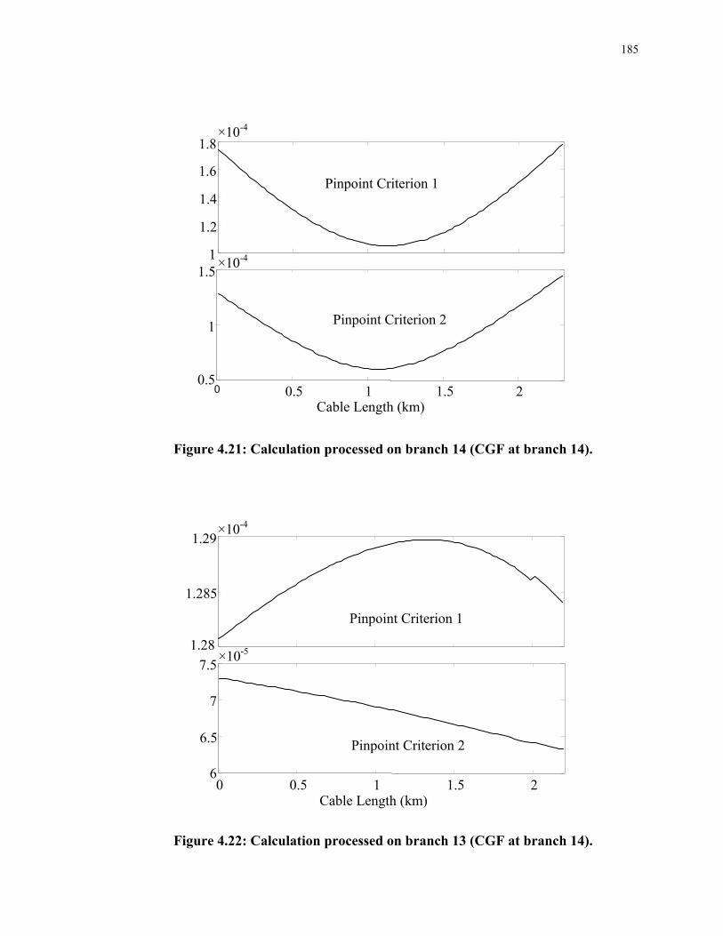
185
Figure 4.21: Calculation processed on branch 14 (CGF at branch 14).
Figure 4.22: Calculation processed on branch 13 (CGF at branch 14).
1.28
1.285
1.29
0 0.5 1 1.5 2 6
6.5
7
7.5×10⁻⁵
Pinpoint Criterion 1
Pinpoint Criterion 2
Cable Length (km)
×10-4
1
1.2
1.4
1.6
1.8
0 0.5 1 1.5 2 0.5
1
1.5
Pinpoint Criterion 1
Pinpoint Criterion 2
×10-4
×10-4
Cable Length (km)
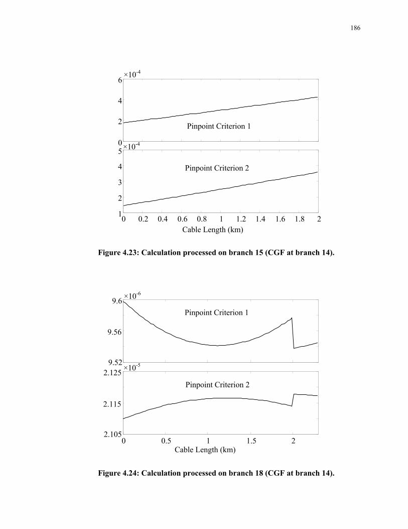
186
Figure 4.23: Calculation processed on branch 15 (CGF at branch 14).
Figure 4.24: Calculation processed on branch 18 (CGF at branch 14).
0
2
4
6
0 0.2 0.4 0.6 0.8 1 1.2 1.4 1.6 1.8 2 1
2
3
4
5
×10-4
×10-4
Cable Length (km)
Pinpoint Criterion 1
Pinpoint Criterion 2
9.52
9.56
9.6
0 0.5 1 1.5 2 2.105
2.115
2.125
×10-6
×10-5
Pinpoint Criterion 2
Pinpoint Criterion 1
Cable Length (km)
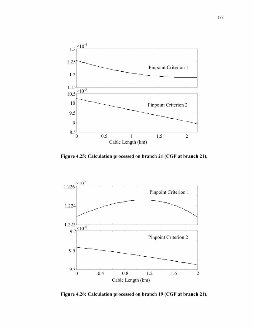
187
Figure 4.25: Calculation processed on branch 21 (CGF at branch 21).
Figure 4.26: Calculation processed on branch 19 (CGF at branch 21).
1.15
1.2
1.25
1.3
0 0.5 1 1.5 2 8.5
9
9.5
10
10.5 ×10-5
×10-4
Pinpoint Criterion 1
Pinpoint Criterion 2
Cable Length (km)
1.222
1.224
1.226
0 0.4 0.8 1.2 1.6 2 9.3
9.5
9.7
×10-4
×10-5
Pinpoint Criterion 1
Pinpoint Criterion 2
Cable Length (km)
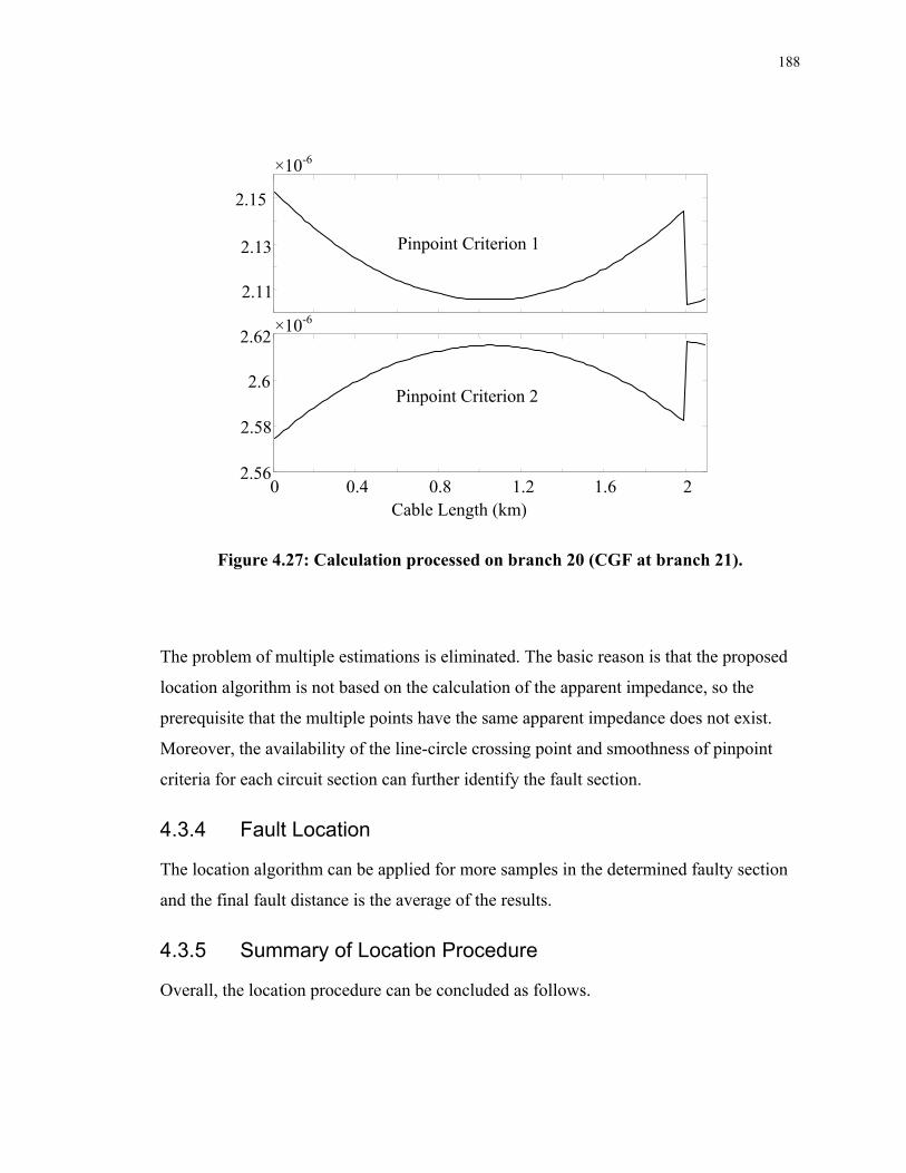
188
Figure 4.27: Calculation processed on branch 20 (CGF at branch 21).
The problem of multiple estimations is eliminated. The basic reason is that the proposed
location algorithm is not based on the calculation of the apparent impedance, so the
prerequisite that the multiple points have the same apparent impedance does not exist.
Moreover, the availability of the line-circle crossing point and smoothness of pinpoint
criteria for each circuit section can further identify the fault section.
4.3.4 Fault Location
The location algorithm can be applied for more samples in the determined faulty section
and the final fault distance is the average of the results.
4.3.5 Summary of Location Procedure
Overall, the location procedure can be concluded as follows.
2.11
2.13
2.15
0 0.4 0.8 1.2 1.6 2 2.56
2.58
2.6
2.62
×10-6
×10-6
Pinpoint Criterion 2
Pinpoint Criterion 1
Cable Length (km)
189
Step 1: The state estimation problem is regularly solved by SQP methods in DMS,
and the voltage at each node is estimated. Then the branch current of each branch,
injected load at each node and seen impedance behind each circuit are calculated.
This step is explained in Section 4.3.1.
Step 2: Upon the occurrence of a fault, the voltages and currents at the sending
terminal of each circuit section are estimated with the assumption that the fault may
occur at this certain section. The employed quantities are the real measurements
during the fault, and estimated load impedance at each node obtained in Step 1. This
step is explained in Section 4.3.2.
Step 3: The faulty section has been assumed, the voltage and current have been
estimated in Step 2, and the seen impedance has been estimated in Step1. The
proposed location algorithm in Chapter 3 is applied for each cable section, starting
from the source. The true faulty section would be selected. This step is explained in
Section 4.3.3.
Step 4: The location algorithm can be applied for more samples in the determined
faulty section as mentioned in Section 4.3.4.
With respect to the three emerging issues mentioned in Section 4.1.3, the first issue is
resolved in Step 2, the second one in Step 1 and the third one in Step 3.
4.4 Application of Static Response Load Model
The above algorithm is based on the assumption that the load model is the constant
impedance. Similarly to Section 3.9.2, the effect of the static response type models will
be investigated. This load model is introduced in Section 1.3.3 and [39], and given as,
2 2
0 0
n np qV VY G jBr rV V
− −= + (4.43)
The Gr and Br can be estimated by the prefault voltage and current obtained from the
state estimation.
190
The voltage V in Equation (4.43) is the voltage at the load terminal during fault, and its
magnitude can be approximately estimated by,
preVlL D pre preV V V Vf s rL preVr
− = − −
(4.44)
where D is the fault distance, L is the cable length. presV is the prefault voltage at the
sending terminal, prerV is the prefault voltage at the receiving terminal, pre
lV is the
prefault voltage at the load point, all of them are estimated by the state estimation
method. Vf is the fault voltage calculated in the location process.
Since the load impedance is changed during the fault, the seen impedance calculated by
the prefault quantities cannot be used. However, it can be estimated by Equation (4.42)
during the fault. Due to the large computation in such situation, the constant parameters
used in the calculation can be preprocessed and stored in the database.
4.5 Simulations
4.5.1 Test System and Cases
A radial underground distribution network shown in Figure 4.2 is used to examine the
state estimation algorithm and fault location algorithm. The test system has the following
aspects:
31 buses.
23 three-phase feeders or laterals and 7 single-phase laterals.
9 three-phase, 2 double-phase and 9 single-phase loads.
All circuits are composed of underground cables with sheaths grounded at the
sending terminal of circuit sections.
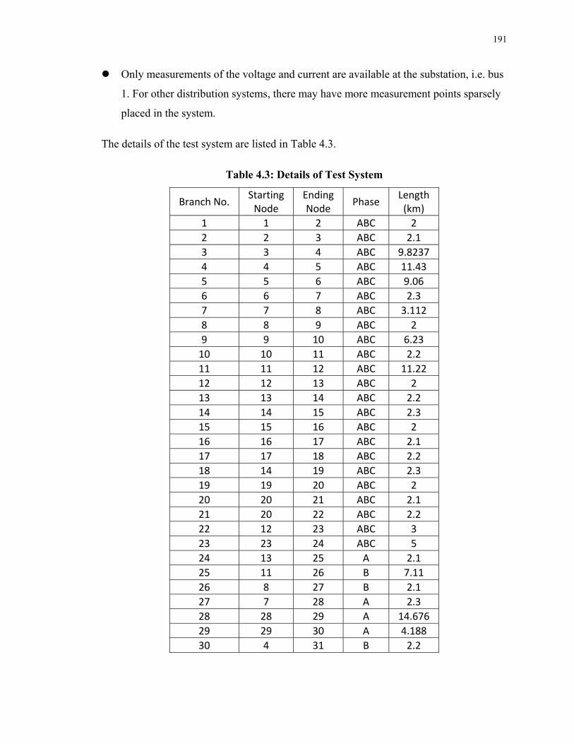
191
Only measurements of the voltage and current are available at the substation, i.e. bus
1. For other distribution systems, there may have more measurement points sparsely
placed in the system.
The details of the test system are listed in Table 4.3.
Table 4.3: Details of Test System
Branch No. Starting Node
Ending Node Phase Length
(km) 1 1 2 ABC 2 2 2 3 ABC 2.1 3 3 4 ABC 9.8237 4 4 5 ABC 11.43 5 5 6 ABC 9.06 6 6 7 ABC 2.3 7 7 8 ABC 3.112 8 8 9 ABC 2 9 9 10 ABC 6.23
10 10 11 ABC 2.2 11 11 12 ABC 11.22 12 12 13 ABC 2 13 13 14 ABC 2.2 14 14 15 ABC 2.3 15 15 16 ABC 2 16 16 17 ABC 2.1 17 17 18 ABC 2.2 18 14 19 ABC 2.3 19 19 20 ABC 2 20 20 21 ABC 2.1 21 20 22 ABC 2.2 22 12 23 ABC 3 23 23 24 ABC 5 24 13 25 A 2.1 25 11 26 B 7.11 26 8 27 B 2.1 27 7 28 A 2.3 28 28 29 A 14.676 29 29 30 A 4.188 30 4 31 B 2.2
192
In order to apply the proposed state estimation technique, a set of initial load patterns
(LP) should be assigned as the load pseudo measurements. Therefore, seven load patterns
given below are introduced by uniformly or randomly perturbing the true loads within a
range.
LP1: higher within 4~6%.
LP2: higher within 0~5%.
LP3: higher within 5~10%.
LP4: higher within 5~15%.
LP5: within -5~5%.
LP6: within -10~10%.
LP7: within -20~20%.
The patterns LP1-LP4 demonstrate the uniform load profiles, which have a uniformly
positive bias regarding to the true loads. The patterns LP5-LP7 represent the generic load
profiles.
The fault cases involve the following variation of parameters and conditions:
Faults occur at each three-phase cable.
Fault distances are fixed at 25%, 50% and 75% length of each cable section.
Fault resistances are fixed as 4 ohm.
Three fault scenarios are respectively involved for each fault point.
The location algorithm is processed for each load pattern.
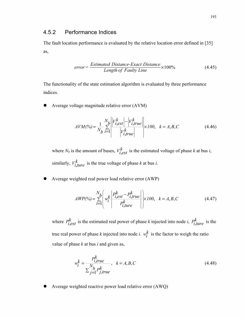
193
4.5.2 Performance Indices
The fault location performance is evaluated by the relative location error defined in [35]
as,
100%Estimated Distance-Exact Distance
error =Length of Faulty Line
× (4.45)
The functionality of the state estimation algorithm is evaluated by three performance
indices.
Average voltage magnitude relative error (AVM)
, ,1 , , ,1 ,
k kN V Vb i est i trueAVM(%) 100 k A B C
N ki Vb i true
−= × =
= (4.46)
where Nb is the amount of buses, ,kVi est is the estimated voltage of phase k at bus i,
similarly, ,kVi ture is the true voltage of phase k at bus i.
Average weighted real power load relative error (AWP)
, , , , ,1 ,
k kN P Pb i est i truekAWP(%) w 100 k A B Ci ki Pi ture
−= × =
= (4.47)
where ,kPi est is the estimated real power of phase k injected into node i, ,
kPi ture is the
true real power of phase k injected into node i. kwi is the factor to weigh the ratio
value of phase k at bus i and given as,
, , , ,
,1
kPi truekw k A B Ci N kb Pj truej
= = =
(4.48)
Average weighted reactive power load relative error (AWQ)
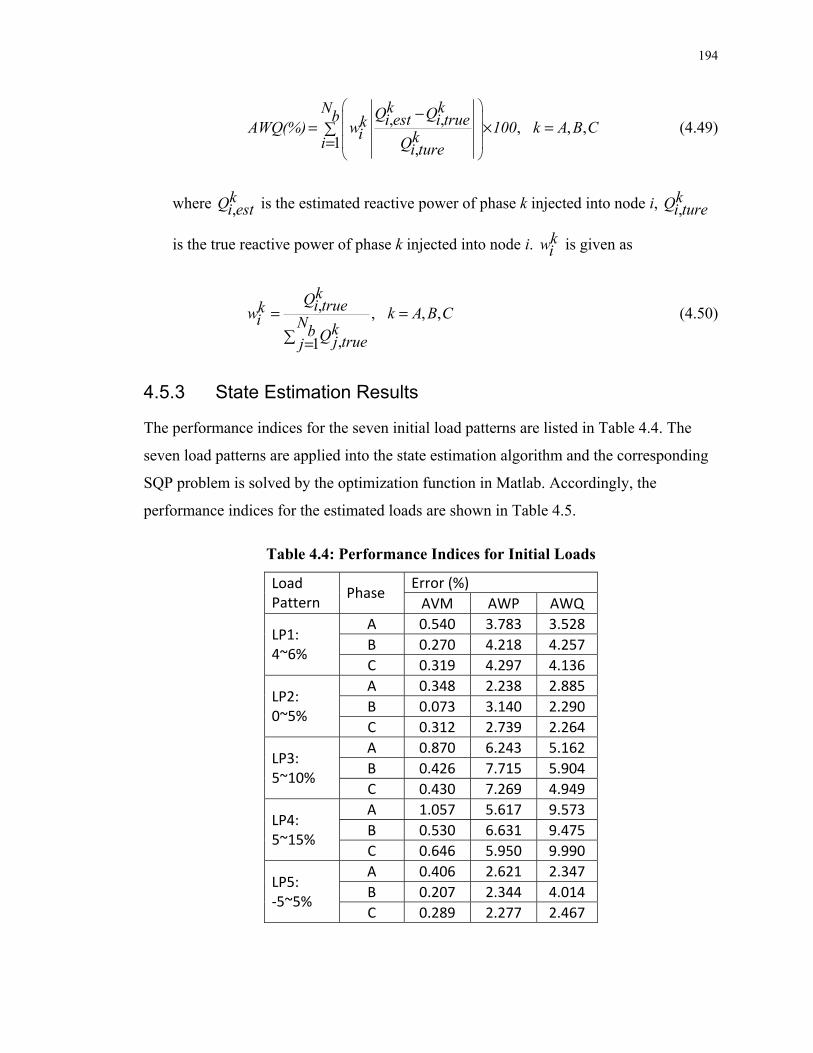
194
, , , , ,1 ,
k kN Q Qb i est i truekAWQ(%) w 100 k A B Ci ki Qi ture
−= × =
= (4.49)
where ,kQi est is the estimated reactive power of phase k injected into node i, ,
kQi ture
is the true reactive power of phase k injected into node i. kwi is given as
, , , ,
,1
kQi truekw k A B Ci N kb Q j truej
= = =
(4.50)
4.5.3 State Estimation Results
The performance indices for the seven initial load patterns are listed in Table 4.4. The
seven load patterns are applied into the state estimation algorithm and the corresponding
SQP problem is solved by the optimization function in Matlab. Accordingly, the
performance indices for the estimated loads are shown in Table 4.5.
Table 4.4: Performance Indices for Initial Loads
Error (%) Load Pattern Phase
AVM AWP AWQ A 0.540 3.783 3.528 B 0.270 4.218 4.257 LP1:
4~6% C 0.319 4.297 4.136 A 0.348 2.238 2.885 B 0.073 3.140 2.290 LP2:
0~5% C 0.312 2.739 2.264 A 0.870 6.243 5.162 B 0.426 7.715 5.904 LP3:
5~10% C 0.430 7.269 4.949 A 1.057 5.617 9.573 B 0.530 6.631 9.475 LP4:
5~15% C 0.646 5.950 9.990 A 0.406 2.621 2.347 B 0.207 2.344 4.014 LP5:
-5~5% C 0.289 2.277 2.467
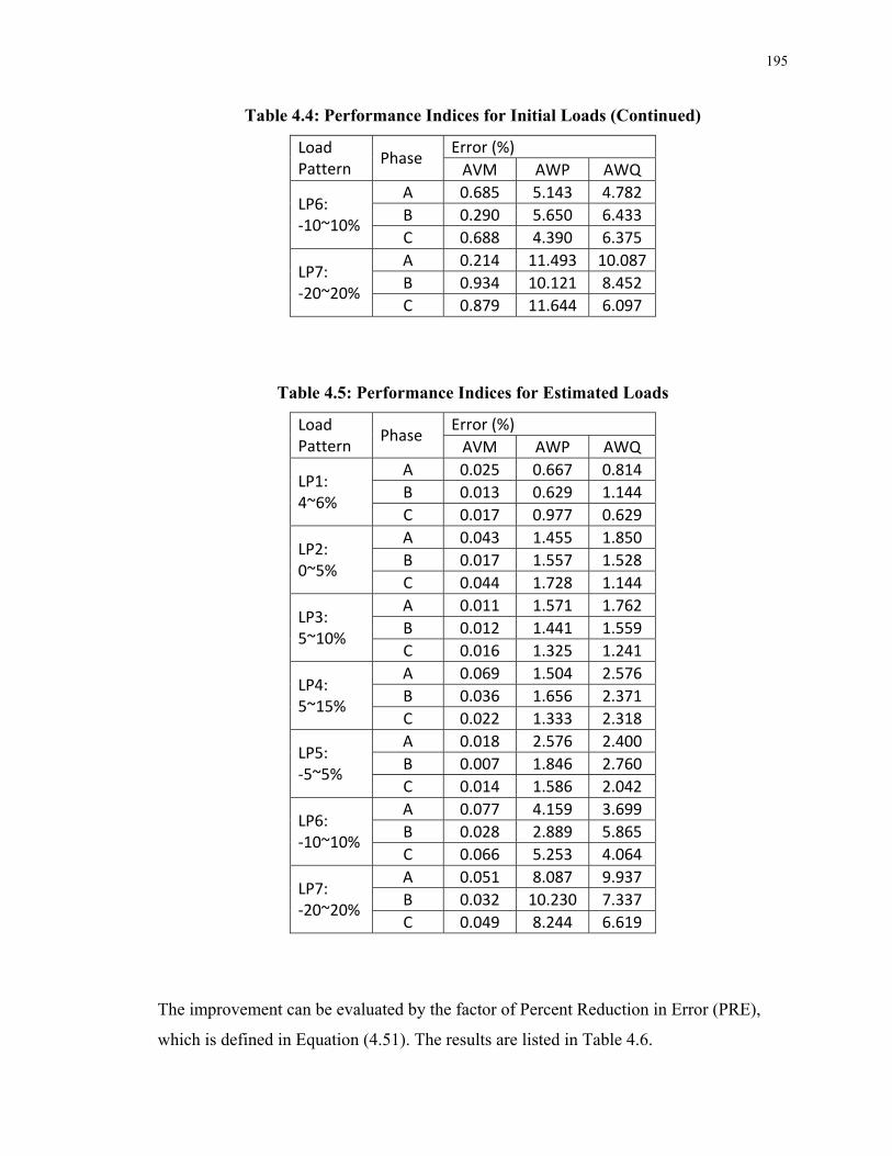
195
Table 4.4: Performance Indices for Initial Loads (Continued)
Error (%) Load Pattern Phase
AVM AWP AWQ A 0.685 5.143 4.782 B 0.290 5.650 6.433 LP6:
-10~10% C 0.688 4.390 6.375 A 0.214 11.493 10.087 B 0.934 10.121 8.452 LP7:
-20~20% C 0.879 11.644 6.097
Table 4.5: Performance Indices for Estimated Loads
Error (%) Load Pattern Phase
AVM AWP AWQ A 0.025 0.667 0.814 B 0.013 0.629 1.144 LP1:
4~6% C 0.017 0.977 0.629 A 0.043 1.455 1.850 B 0.017 1.557 1.528 LP2:
0~5% C 0.044 1.728 1.144 A 0.011 1.571 1.762 B 0.012 1.441 1.559 LP3:
5~10% C 0.016 1.325 1.241 A 0.069 1.504 2.576 B 0.036 1.656 2.371 LP4:
5~15% C 0.022 1.333 2.318 A 0.018 2.576 2.400 B 0.007 1.846 2.760 LP5:
-5~5% C 0.014 1.586 2.042 A 0.077 4.159 3.699 B 0.028 2.889 5.865 LP6:
-10~10% C 0.066 5.253 4.064 A 0.051 8.087 9.937 B 0.032 10.230 7.337 LP7:
-20~20% C 0.049 8.244 6.619
The improvement can be evaluated by the factor of Percent Reduction in Error (PRE),
which is defined in Equation (4.51). The results are listed in Table 4.6.
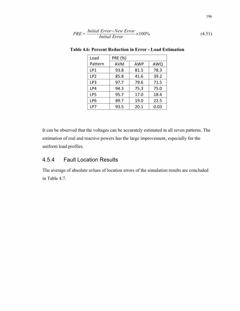
196
100%Initial Error New Error
PRE =Initial Error
− × (4.51)
Table 4.6: Percent Reduction in Error - Load Estimation
PRE (%) Load Pattern AVM AWP AWQ LP1 93.8 81.5 78.3 LP2 85.8 41.6 39.2 LP3 97.7 79.6 71.5 LP4 94.3 75.3 75.0 LP5 95.7 17.0 18.4 LP6 89.7 19.0 22.5 LP7 93.5 20.1 0.03
It can be observed that the voltages can be accurately estimated in all seven patterns. The
estimation of real and reactive powers has the large improvement, especially for the
uniform load profiles.
4.5.4 Fault Location Results
The average of absolute avlues of location errors of the simulation results are concluded
in Table 4.7.
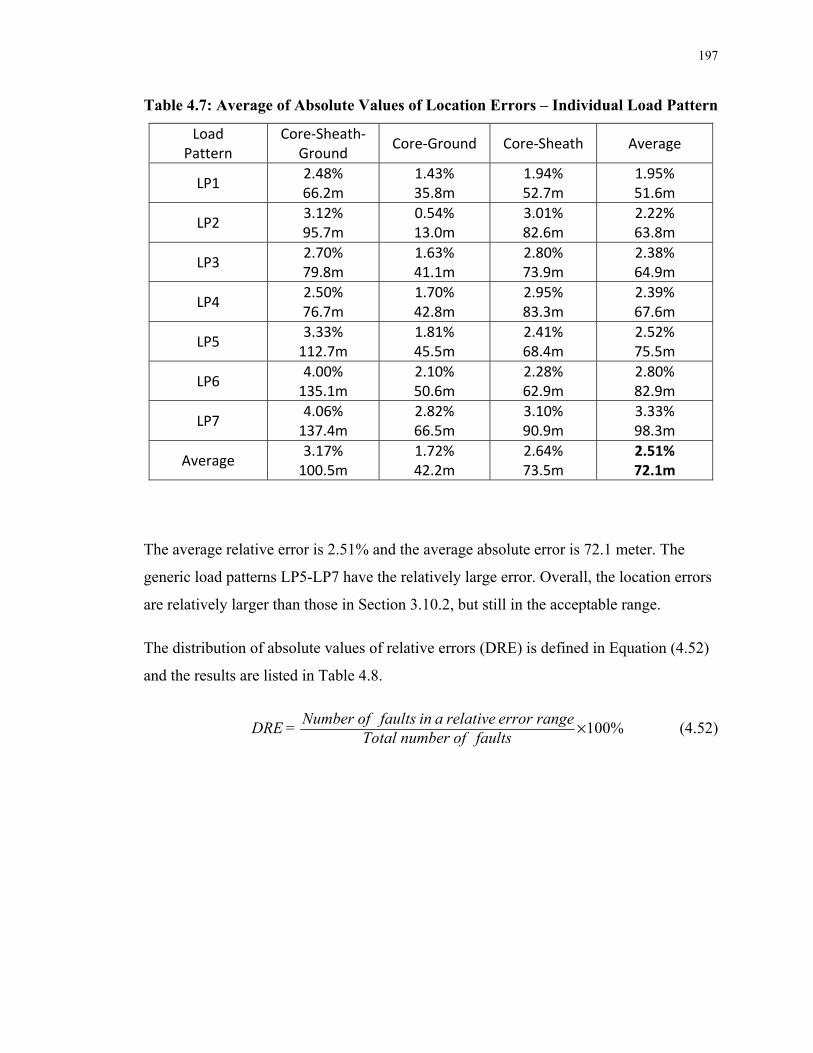
197
Table 4.7: Average of Absolute Values of Location Errors – Individual Load Pattern
Load Pattern
Core-Sheath- Ground Core-Ground Core-Sheath Average
LP1 2.48% 66.2m
1.43% 35.8m
1.94% 52.7m
1.95% 51.6m
LP2 3.12% 95.7m
0.54% 13.0m
3.01% 82.6m
2.22% 63.8m
LP3 2.70% 79.8m
1.63% 41.1m
2.80% 73.9m
2.38% 64.9m
LP4 2.50% 76.7m
1.70% 42.8m
2.95% 83.3m
2.39% 67.6m
LP5 3.33% 112.7m
1.81% 45.5m
2.41% 68.4m
2.52% 75.5m
LP6 4.00% 135.1m
2.10% 50.6m
2.28% 62.9m
2.80% 82.9m
LP7 4.06% 137.4m
2.82% 66.5m
3.10% 90.9m
3.33% 98.3m
Average 3.17% 100.5m
1.72% 42.2m
2.64% 73.5m
2.51% 72.1m
The average relative error is 2.51% and the average absolute error is 72.1 meter. The
generic load patterns LP5-LP7 have the relatively large error. Overall, the location errors
are relatively larger than those in Section 3.10.2, but still in the acceptable range.
The distribution of absolute values of relative errors (DRE) is defined in Equation (4.52)
and the results are listed in Table 4.8.
100%Number of faults in a relative error range
DRE =Total number of faults
× (4.52)
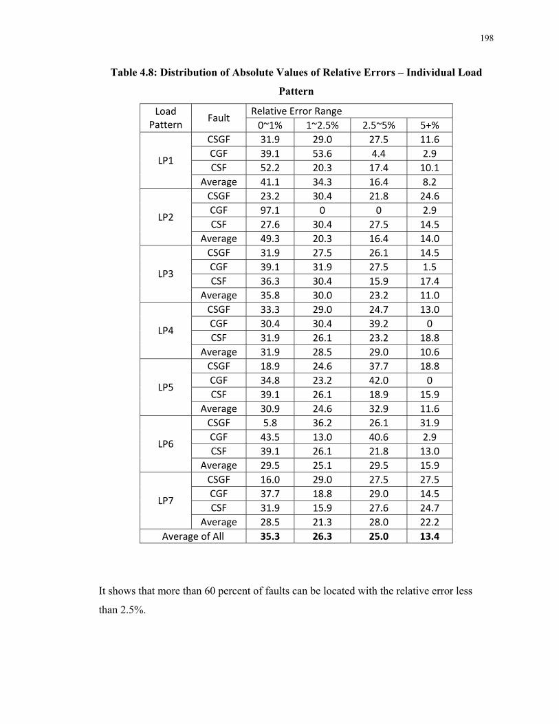
198
Table 4.8: Distribution of Absolute Values of Relative Errors – Individual Load
Pattern
Relative Error Range Load Pattern Fault
0~1% 1~2.5% 2.5~5% 5+% CSGF 31.9 29.0 27.5 11.6 CGF 39.1 53.6 4.4 2.9 CSF 52.2 20.3 17.4 10.1
LP1
Average 41.1 34.3 16.4 8.2 CSGF 23.2 30.4 21.8 24.6 CGF 97.1 0 0 2.9 CSF 27.6 30.4 27.5 14.5
LP2
Average 49.3 20.3 16.4 14.0 CSGF 31.9 27.5 26.1 14.5 CGF 39.1 31.9 27.5 1.5 CSF 36.3 30.4 15.9 17.4
LP3
Average 35.8 30.0 23.2 11.0 CSGF 33.3 29.0 24.7 13.0 CGF 30.4 30.4 39.2 0 CSF 31.9 26.1 23.2 18.8
LP4
Average 31.9 28.5 29.0 10.6 CSGF 18.9 24.6 37.7 18.8 CGF 34.8 23.2 42.0 0 CSF 39.1 26.1 18.9 15.9
LP5
Average 30.9 24.6 32.9 11.6 CSGF 5.8 36.2 26.1 31.9 CGF 43.5 13.0 40.6 2.9 CSF 39.1 26.1 21.8 13.0
LP6
Average 29.5 25.1 29.5 15.9 CSGF 16.0 29.0 27.5 27.5 CGF 37.7 18.8 29.0 14.5 CSF 31.9 15.9 27.6 24.7
LP7
Average 28.5 21.3 28.0 22.2 Average of All 35.3 26.3 25.0 13.4
It shows that more than 60 percent of faults can be located with the relative error less
than 2.5%.
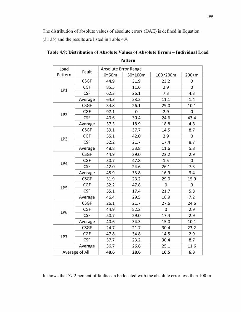
199
The distribution of absolute values of absolute errors (DAE) is defined in Equation
(3.135) and the results are listed in Table 4.9.
Table 4.9: Distribution of Absolute Values of Absolute Errors – Individual Load
Pattern
Absolute Error Range Load Pattern Fault
0~50m 50~100m 100~200m 200+m CSGF 44.9 31.9 23.2 0 CGF 85.5 11.6 2.9 0 CSF 62.3 26.1 7.3 4.3
LP1
Average 64.3 23.2 11.1 1.4 CSGF 34.8 26.1 29.0 10.1 CGF 97.1 0 2.9 0 CSF 40.6 30.4 24.6 43.4
LP2
Average 57.5 18.9 18.8 4.8 CSGF 39.1 37.7 14.5 8.7 CGF 55.1 42.0 2.9 0 CSF 52.2 21.7 17.4 8.7
LP3
Average 48.8 33.8 11.6 5.8 CSGF 44.9 29.0 23.2 2.9 CGF 50.7 47.8 1.5 0 CSF 42.0 24.6 26.1 7.3
LP4
Average 45.9 33.8 16.9 3.4 CSGF 31.9 23.2 29.0 15.9 CGF 52.2 47.8 0 0 CSF 55.1 17.4 21.7 5.8
LP5
Average 46.4 29.5 16.9 7.2 CSGF 26.1 21.7 27.6 24.6 CGF 44.9 52.2 0 2.9 CSF 50.7 29.0 17.4 2.9
LP6
Average 40.6 34.3 15.0 10.1 CSGF 24.7 21.7 30.4 23.2 CGF 47.8 34.8 14.5 2.9 CSF 37.7 23.2 30.4 8.7
LP7
Average 36.7 26.6 25.1 11.6 Average of All 48.6 28.6 16.5 6.3
It shows that 77.2 percent of faults can be located with the absolute error less than 100 m.
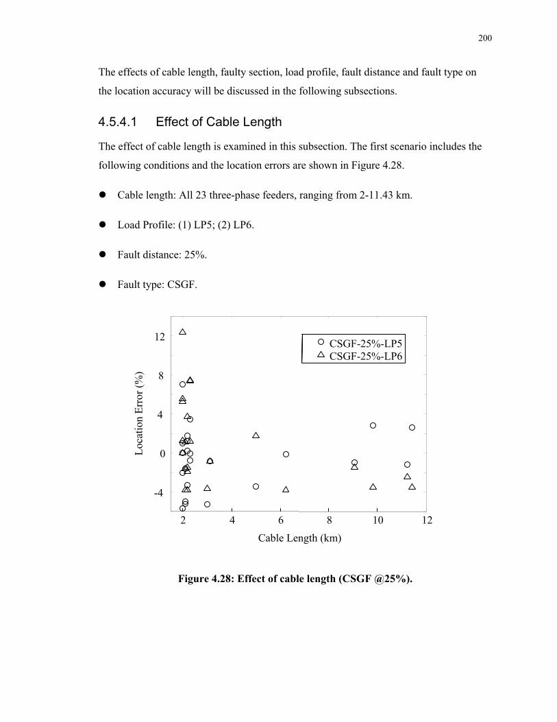
200
The effects of cable length, faulty section, load profile, fault distance and fault type on
the location accuracy will be discussed in the following subsections.
4.5.4.1 Effect of Cable Length
The effect of cable length is examined in this subsection. The first scenario includes the
following conditions and the location errors are shown in Figure 4.28.
Cable length: All 23 three-phase feeders, ranging from 2-11.43 km.
Load Profile: (1) LP5; (2) LP6.
Fault distance: 25%.
Fault type: CSGF.
Figure 4.28: Effect of cable length (CSGF @25%).
2 4 6 8 10 12
-4
0
4
8
12
CSGF-25%-LP5 CSGF-25%-LP6
Cable Length (km)
Loc
atio
n E
rror
(%
)
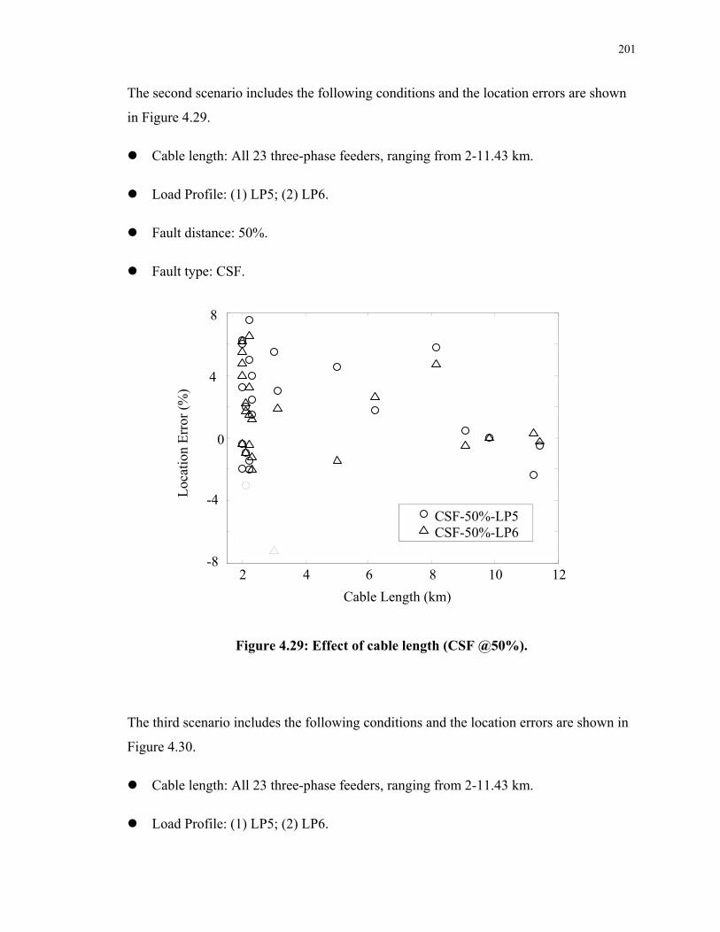
201
The second scenario includes the following conditions and the location errors are shown
in Figure 4.29.
Cable length: All 23 three-phase feeders, ranging from 2-11.43 km.
Load Profile: (1) LP5; (2) LP6.
Fault distance: 50%.
Fault type: CSF.
Figure 4.29: Effect of cable length (CSF @50%).
The third scenario includes the following conditions and the location errors are shown in
Figure 4.30.
Cable length: All 23 three-phase feeders, ranging from 2-11.43 km.
Load Profile: (1) LP5; (2) LP6.
2 4 6 8 10 12 -8
-4
0
4
8
Cable Length (km)
CSF-50%-LP5 CSF-50%-LP6
Loc
atio
n E
rror
(%
)
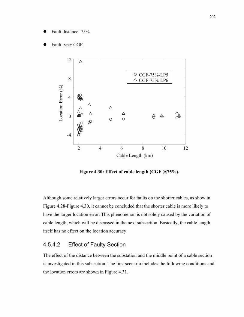
202
Fault distance: 75%.
Fault type: CGF.
Figure 4.30: Effect of cable length (CGF @75%).
Although some relatively larger errors occur for faults on the shorter cables, as show in
Figure 4.28-Figure 4.30, it cannot be concluded that the shorter cable is more likely to
have the larger location error. This phenomenon is not solely caused by the variation of
cable length, which will be discussed in the next subsection. Basically, the cable length
itself has no effect on the location accuracy.
4.5.4.2 Effect of Faulty Section
The effect of the distance between the substation and the middle point of a cable section
is investigated in this subsection. The first scenario includes the following conditions and
the location errors are shown in Figure 4.31.
2 4 6 8 10 12
-4
0
4
8
12
CGF-75%-LP5 CGF-75%-LP6
Cable Length (km)
Loc
atio
n E
rror
(%
)
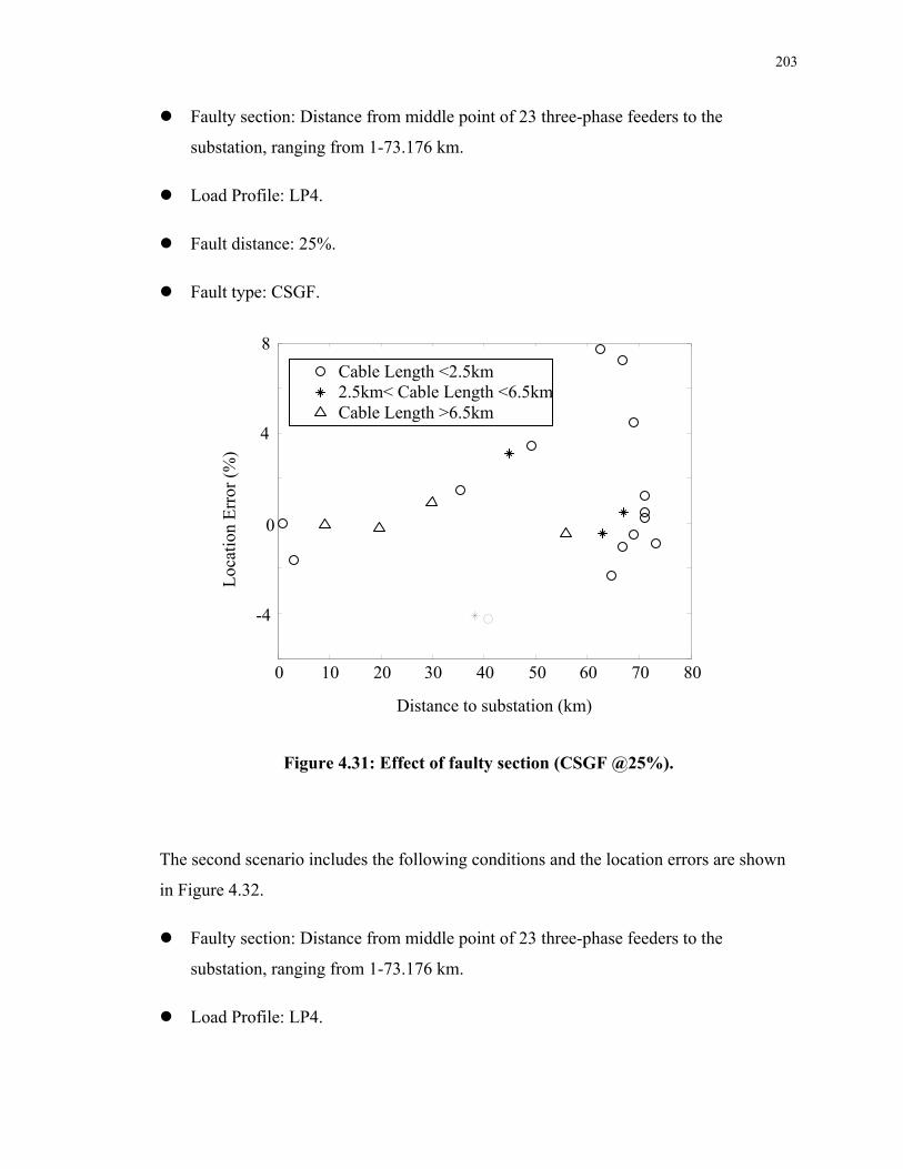
203
Faulty section: Distance from middle point of 23 three-phase feeders to the
substation, ranging from 1-73.176 km.
Load Profile: LP4.
Fault distance: 25%.
Fault type: CSGF.
Figure 4.31: Effect of faulty section (CSGF @25%).
The second scenario includes the following conditions and the location errors are shown
in Figure 4.32.
Faulty section: Distance from middle point of 23 three-phase feeders to the
substation, ranging from 1-73.176 km.
Load Profile: LP4.
0 10 20 30 40 50 60 70 80
-4
0
4
8
Cable Length <2.5km 2.5km< Cable Length <6.5kmCable Length >6.5km
Distance to substation (km)
Loc
atio
n E
rror
(%
)
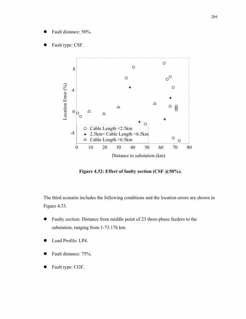
204
Fault distance: 50%.
Fault type: CSF.
Figure 4.32: Effect of faulty section (CSF @50%).
The third scenario includes the following conditions and the location errors are shown in
Figure 4.33.
Faulty section: Distance from middle point of 23 three-phase feeders to the
substation, ranging from 1-73.176 km.
Load Profile: LP4.
Fault distance: 75%.
Fault type: CGF.
0 10 20 30 40 50 60 70 80
-4
0
4
8
Distance to substation (km)
Loc
atio
n E
rror
(%
)
Cable Length <2.5km 2.5km< Cable Length <6.5kmCable Length >6.5km
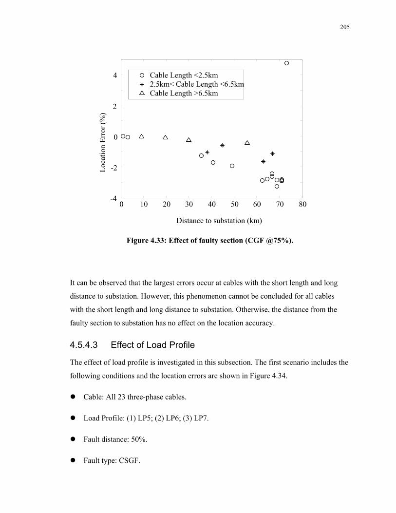
205
Figure 4.33: Effect of faulty section (CGF @75%).
It can be observed that the largest errors occur at cables with the short length and long
distance to substation. However, this phenomenon cannot be concluded for all cables
with the short length and long distance to substation. Otherwise, the distance from the
faulty section to substation has no effect on the location accuracy.
4.5.4.3 Effect of Load Profile
The effect of load profile is investigated in this subsection. The first scenario includes the
following conditions and the location errors are shown in Figure 4.34.
Cable: All 23 three-phase cables.
Load Profile: (1) LP5; (2) LP6; (3) LP7.
Fault distance: 50%.
Fault type: CSGF.
0 10 20 30 40 50 60 70 80 -4
-2
0
2
4
Distance to substation (km)
Loc
atio
n E
rror
(%
)
Cable Length <2.5km 2.5km< Cable Length <6.5kmCable Length >6.5km
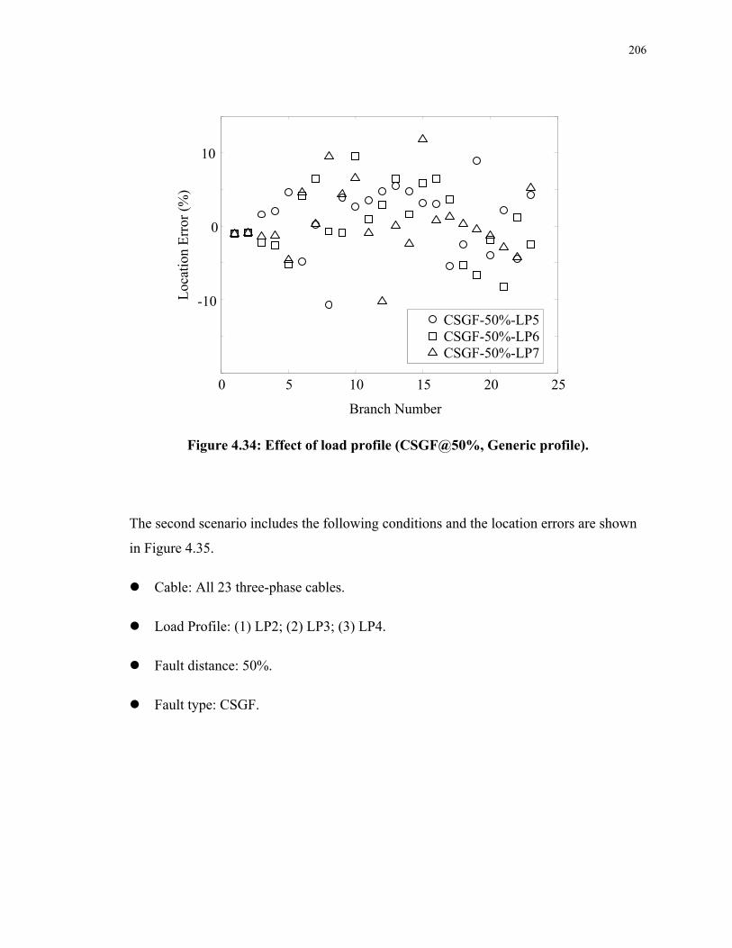
206
Figure 4.34: Effect of load profile (CSGF@50%, Generic profile).
The second scenario includes the following conditions and the location errors are shown
in Figure 4.35.
Cable: All 23 three-phase cables.
Load Profile: (1) LP2; (2) LP3; (3) LP4.
Fault distance: 50%.
Fault type: CSGF.
0 5 10 15 20 25
-10
0
10
CSGF-50%-LP5 CSGF-50%-LP6 CSGF-50%-LP7
Branch Number
Loc
atio
n E
rror
(%
)
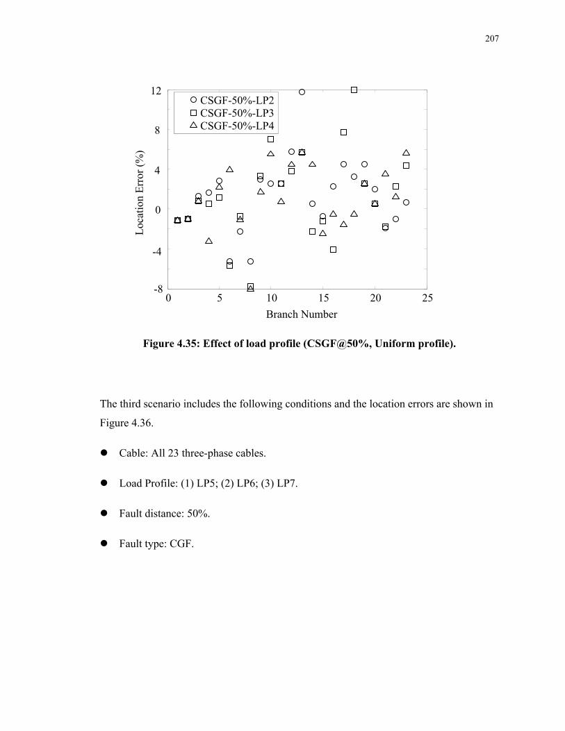
207
Figure 4.35: Effect of load profile (CSGF@50%, Uniform profile).
The third scenario includes the following conditions and the location errors are shown in
Figure 4.36.
Cable: All 23 three-phase cables.
Load Profile: (1) LP5; (2) LP6; (3) LP7.
Fault distance: 50%.
Fault type: CGF.
0 5 10 15 20 25 -8
-4
0
4
8
12
CSGF-50%-LP2 CSGF-50%-LP3 CSGF-50%-LP4
Branch Number
Loc
atio
n E
rror
(%
)
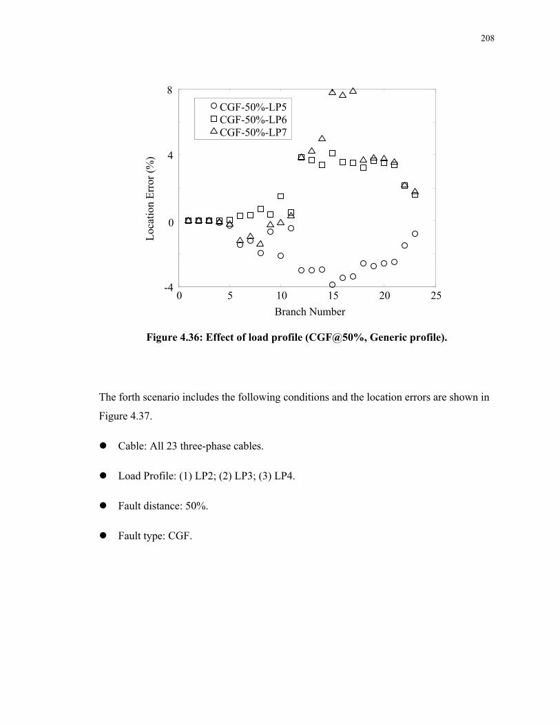
208
Figure 4.36: Effect of load profile (CGF@50%, Generic profile).
The forth scenario includes the following conditions and the location errors are shown in
Figure 4.37.
Cable: All 23 three-phase cables.
Load Profile: (1) LP2; (2) LP3; (3) LP4.
Fault distance: 50%.
Fault type: CGF.
0 5 10 15 20 25 -4
0
4
8
CGF-50%-LP5 CGF-50%-LP6 CGF-50%-LP7
Branch Number
Loc
atio
n E
rror
(%
)
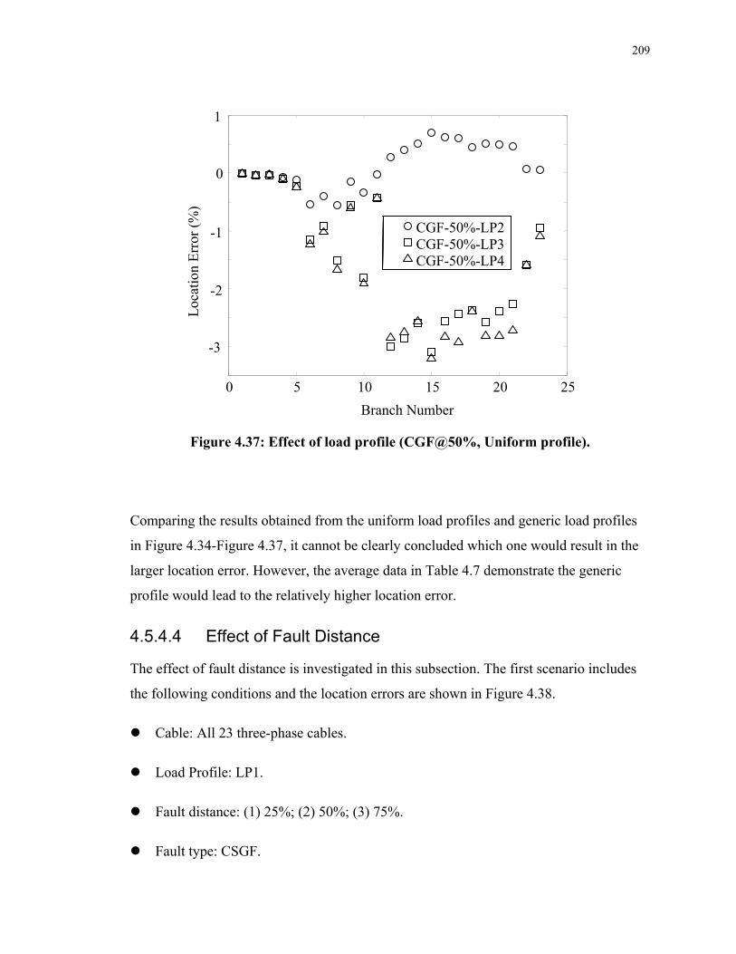
209
Figure 4.37: Effect of load profile (CGF@50%, Uniform profile).
Comparing the results obtained from the uniform load profiles and generic load profiles
in Figure 4.34-Figure 4.37, it cannot be clearly concluded which one would result in the
larger location error. However, the average data in Table 4.7 demonstrate the generic
profile would lead to the relatively higher location error.
4.5.4.4 Effect of Fault Distance
The effect of fault distance is investigated in this subsection. The first scenario includes
the following conditions and the location errors are shown in Figure 4.38.
Cable: All 23 three-phase cables.
Load Profile: LP1.
Fault distance: (1) 25%; (2) 50%; (3) 75%.
Fault type: CSGF.
0 5 10 15 20 25
-3
-2
-1
0
1
CGF-50%-LP2 CGF-50%-LP3 CGF-50%-LP4
Branch Number
Loc
atio
n E
rror
(%
)
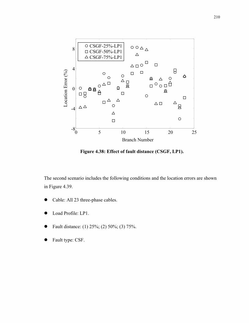
210
Figure 4.38: Effect of fault distance (CSGF, LP1).
The second scenario includes the following conditions and the location errors are shown
in Figure 4.39.
Cable: All 23 three-phase cables.
Load Profile: LP1.
Fault distance: (1) 25%; (2) 50%; (3) 75%.
Fault type: CSF.
0 5 10 15 20 25 -8
-4
0
4
8
CSGF-25%-LP1 CSGF-50%-LP1 CSGF-75%-LP1
Branch Number
Loc
atio
n E
rror
(%
)
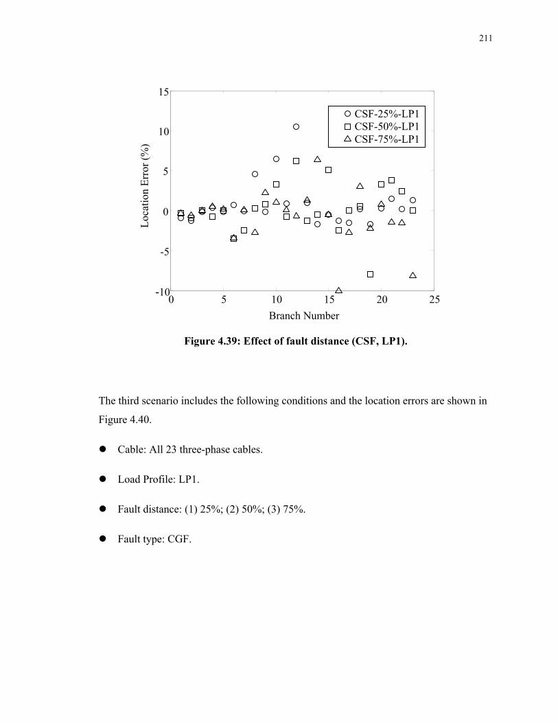
211
Figure 4.39: Effect of fault distance (CSF, LP1).
The third scenario includes the following conditions and the location errors are shown in
Figure 4.40.
Cable: All 23 three-phase cables.
Load Profile: LP1.
Fault distance: (1) 25%; (2) 50%; (3) 75%.
Fault type: CGF.
0 5 10 15 20 25 -10
-5
0
5
10
15
CSF-25%-LP1 CSF-50%-LP1 CSF-75%-LP1
Branch Number
Loc
atio
n E
rror
(%
)
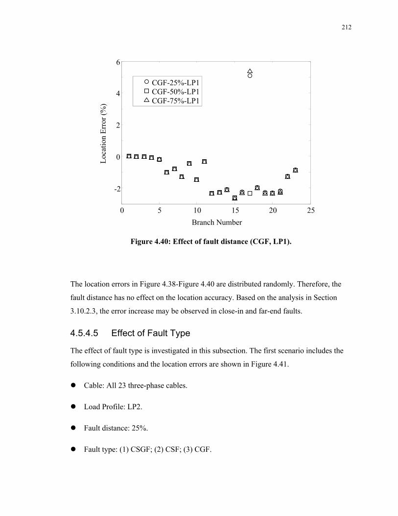
212
Figure 4.40: Effect of fault distance (CGF, LP1).
The location errors in Figure 4.38-Figure 4.40 are distributed randomly. Therefore, the
fault distance has no effect on the location accuracy. Based on the analysis in Section
3.10.2.3, the error increase may be observed in close-in and far-end faults.
4.5.4.5 Effect of Fault Type
The effect of fault type is investigated in this subsection. The first scenario includes the
following conditions and the location errors are shown in Figure 4.41.
Cable: All 23 three-phase cables.
Load Profile: LP2.
Fault distance: 25%.
Fault type: (1) CSGF; (2) CSF; (3) CGF.
0 5 10 15 20 25
-2
0
2
4
6
CGF-25%-LP1 CGF-50%-LP1 CGF-75%-LP1
Loc
atio
n E
rror
(%
)
Branch Number
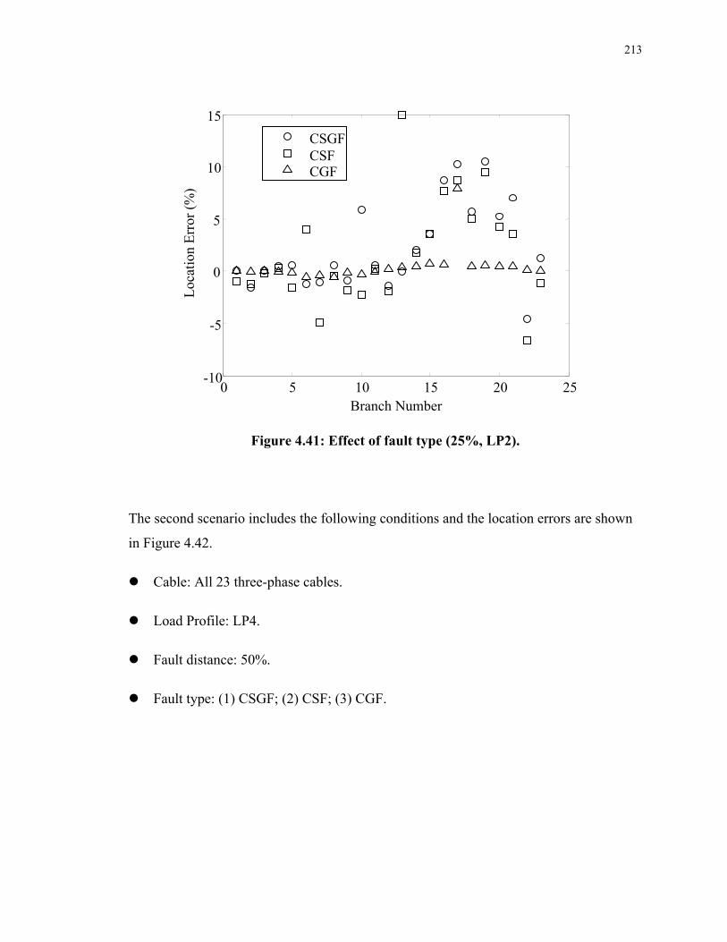
213
Figure 4.41: Effect of fault type (25%, LP2).
The second scenario includes the following conditions and the location errors are shown
in Figure 4.42.
Cable: All 23 three-phase cables.
Load Profile: LP4.
Fault distance: 50%.
Fault type: (1) CSGF; (2) CSF; (3) CGF.
0 5 10 15 20 25 -10
-5
0
5
10
15
CSGFCSFCGF
Loc
atio
n E
rror
(%
)
Branch Number
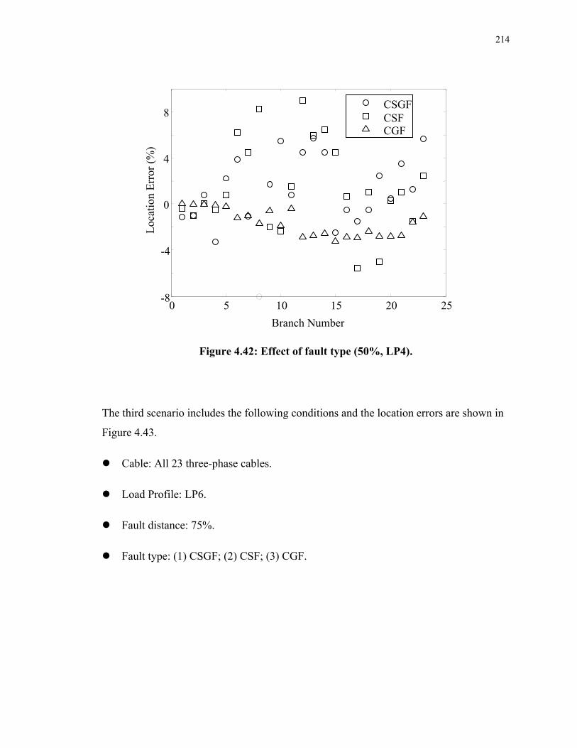
214
Figure 4.42: Effect of fault type (50%, LP4).
The third scenario includes the following conditions and the location errors are shown in
Figure 4.43.
Cable: All 23 three-phase cables.
Load Profile: LP6.
Fault distance: 75%.
Fault type: (1) CSGF; (2) CSF; (3) CGF.
0 5 10 15 20 25 -8
-4
0
4
8
CSGF CSFCGF
Branch Number
Loc
atio
n E
rror
(%
)
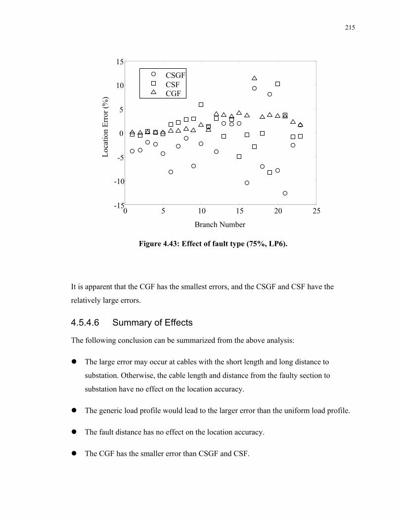
215
Figure 4.43: Effect of fault type (75%, LP6).
It is apparent that the CGF has the smallest errors, and the CSGF and CSF have the
relatively large errors.
4.5.4.6 Summary of Effects
The following conclusion can be summarized from the above analysis:
The large error may occur at cables with the short length and long distance to
substation. Otherwise, the cable length and distance from the faulty section to
substation have no effect on the location accuracy.
The generic load profile would lead to the larger error than the uniform load profile.
The fault distance has no effect on the location accuracy.
The CGF has the smaller error than CSGF and CSF.
0 5 10 15 20 25 -15
-10
-5
0
5
10
15
CSGFCSFCGF
Branch Number
Loc
atio
n E
rror
(%
)

216
4.5.4.7 More Accurate Results
The above simulation results are based on one certain load profile individually. However,
there may have several load profiles available for the state estimation and the most
suitable one cannot be readily decided. Therefore, several available load profiles can be
processed for the state estimation and fault location. The final results can be calculated by
averaging.
Three groups are simulated, in which five load profiles are randomly selected from the
seven load patterns. The average of absolute values of location errors of each group are
concluded in Table 4.10.
Table 4.10: Average of Absolute Values of Location Errors – Combination of Load
Patterns
Load Patterns
Core-Sheath- Ground Core-Ground Core-Sheath Average
LP2, 4, 5, 6,7 2.02% 59.5m
0.63% 16.3m
1.65% 45.4m
1.43% 40.4m
LP2, 3, 4, 5, 6 1.94% 58.3m
1.14% 28.9m
1.4% 38.1m
1.49% 41.8m
LP1, 2, 3, 6, 7 2.08% 62.2m
0.68% 17.0m
1.37% 36.7m
1.38% 38.6m
The percent reduction in error is used to evaluate the improvement in location errors, as
shown in Table 4.11. It can be found that, in average, both relative and absolute errors are
reduced by more than 40%.
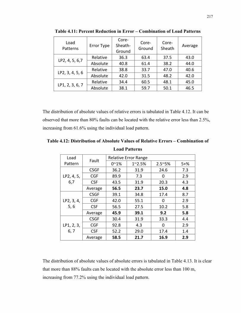
217
Table 4.11: Percent Reduction in Error – Combination of Load Patterns
Load Patterns Error Type
Core- Sheath- Ground
Core- Ground
Core- Sheath Average
Relative 36.3 63.4 37.5 43.0 LP2, 4, 5, 6,7 Absolute 40.8 61.4 38.2 44.0 Relative 38.8 33.7 47.0 40.6 LP2, 3, 4, 5, 6 Absolute 42.0 31.5 48.2 42.0 Relative 34.4 60.5 48.1 45.0 LP1, 2, 3, 6, 7 Absolute 38.1 59.7 50.1 46.5
The distribution of absolute values of relative errors is tabulated in Table 4.12. It can be
observed that more than 80% faults can be located with the relative error less than 2.5%,
increasing from 61.6% using the individual load pattern.
Table 4.12: Distribution of Absolute Values of Relative Errors – Combination of
Load Patterns
Relative Error Range Load Pattern Fault
0~1% 1~2.5% 2.5~5% 5+% CSGF 36.2 31.9 24.6 7.3 CGF 89.9 7.3 0 2.9 CSF 43.5 31.9 20.3 4.3
LP2, 4, 5, 6,7
Average 56.5 23.7 15.0 4.8 CSGF 39.1 34.8 17.4 8.7 CGF 42.0 55.1 0 2.9 CSF 56.5 27.5 10.2 5.8
LP2, 3, 4, 5, 6
Average 45.9 39.1 9.2 5.8 CSGF 30.4 31.9 33.3 4.4 CGF 92.8 4.3 0 2.9 CSF 52.2 29.0 17.4 1.4
LP1, 2, 3, 6, 7
Average 58.5 21.7 16.9 2.9
The distribution of absolute values of absolute errors is tabulated in Table 4.13. It is clear
that more than 88% faults can be located with the absolute error less than 100 m,
increasing from 77.2% using the individual load pattern.
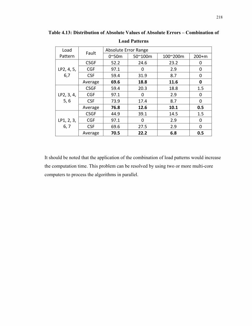
218
Table 4.13: Distribution of Absolute Values of Absolute Errors – Combination of
Load Patterns
Absolute Error Range Load Pattern Fault
0~50m 50~100m 100~200m 200+m CSGF 52.2 24.6 23.2 0 CGF 97.1 0 2.9 0 CSF 59.4 31.9 8.7 0
LP2, 4, 5, 6,7
Average 69.6 18.8 11.6 0 CSGF 59.4 20.3 18.8 1.5 CGF 97.1 0 2.9 0 CSF 73.9 17.4 8.7 0
LP2, 3, 4, 5, 6
Average 76.8 12.6 10.1 0.5 CSGF 44.9 39.1 14.5 1.5 CGF 97.1 0 2.9 0 CSF 69.6 27.5 2.9 0
LP1, 2, 3, 6, 7
Average 70.5 22.2 6.8 0.5
It should be noted that the application of the combination of load patterns would increase
the computation time. This problem can be resolved by using two or more multi-core
computers to process the algorithms in parallel.
219
Chapter 5
5 Conclusions and Future Works
Three schemes have been developed in this thesis, i.e. incipient fault detection for
distribution cables based on the wavelet analysis and superimposed components, fault
location for distribution cables based on the direct circuit analysis, and state estimation
for underground distribution networks based on the sequential quadratic programming
technique. Then, the proposed fault location algorithm and state estimation method have
been applied together to locate faults in underground distribution networks.
5.1 Conclusions
Based on the methodology of wavelet transform and analysis of superimposed
components, two schemes have been proposed to detect and classify the incipient faults
in underground distribution cables. The following design goals have been achieved for
the schemes.
Easy implementation in the existing digital relays;
High detection and classification accuracy;
Low rate of missing detection, false alarm, and incorrect classification;
Insensitive to fault type, fault location, fault resistance, and fault inception angle
Less dead zone;
Robust to noise, disturbance, and uncertainties;
Configurable for different CT locations;
Configurable for different transformer windings;
Capable to detect and classify in real time.

220
The wavelet-based scheme has the following advantages in terms of the accuracy,
detectability, and identifiability.
Achieving higher detection accuracy, especially for high impedance incipient faults;
Supervising almost entire length of cable, i.e., less detection dead zone;
Detecting and classifying the different fault types;
Detecting and classifying the other transients, such as cold load pickup and capacitor
switching;
Eliminating noise from signals.
The superimposed components-based scheme is particularly designed to detect SLG
incipient faults. In other respects, this method has the following advantages in terms of
the configuration and simplicity.
Performing simple and less computation;
Setting fewer thresholds;
Implementing by easily upgrading firmware.
The wavelet-based scheme can obtain the low rate of missing detection and zero rate of
false alarm in the presence of the various noise levels, fault conditions, transient types
and system configurations. The superimposed components-based scheme is capable of
achieving the zero rates of false alarm and misclassification. The advantages of both
schemes indicate a technical feasibility for practical implementations.
Based on the direct circuit analysis of a two-layer π cable model, a set of fault location
algorithms have been proposed to locate the single phase-related permanent faults in
underground cables. The main characteristics of the location algorithms are concluded as
follows.

221
A two-layer π cable model has been formulated to approximate the behaviors and
characteristics of cables and used to develop the location algorithms.
The various cable characteristics have been taken into account, such as the shunt
capacitance, metallic sheaths, heterogeneity and untransposition.
A set of location algorithms have been developed to cover five bonding methods and
three fault scenarios.
A large number of complex equations in the location algorithms have been solved
effectively and efficiently.
Only fundamental voltage and current phasors measured at substation have been
utilized.
The estimation of load impedance has been proposed and the application of the static
response type load model has been investigated.
The location algorithms are capable to calculate fault resistance.
The location algorithms are capable to determine fault type.
The high location accuracy has been achieved.
The location algorithms are insensitive to fault resistance.
Basically, the location algorithms are insensitive to fault distance except that there
has an error increase for faults closed to the close-in, far-end and crossing points,
which is caused by the model and setting in the simulation software.
There may have relatively large error for CSGF or CSF with SPBR or SPBM,
otherwise, the bonding methods and fault scenarios have no effect on the location
accuracy.
The location algorithms are capable to locate in real time.

222
The state estimation for underground distribution networks has been formulated as a
nonlinear optimization problem and solved by the sequential quadratic programming
method. The proposed location algorithm incorporating with the proposed state
estimation algorithm has the following characteristics.
The state estimation for underground distribution networks has been formulated as a
nonlinear optimization problem and solved by the SQP method.
The shunt capacitance, effect of metallic sheath and bonding method have been taken
into account for the development of the state estimation method.
The laterals and tapped loads have been taken into account.
A section-by-section estimation algorithm combined with the backward/forward
sweep algorithm has been proposed to estimate the nodal voltage and branch current
for each line section. Six sub-algorithms have been applied in the estimation
algorithm.
Only fundamental voltage and current phasors measured at substation have been
utilized.
The state estimation algorithm can accurately estimate the nodal voltages. The
estimation accuracy of load flows is acceptable.
The estimation of the seen impedance behind the faulty section has been discussed
and the application of the static response type load model has been investigated.
The state estimation algorithm can provide necessary information for the location
algorithms.
The faulty section can be determined.
The location accuracy is acceptable.

223
Basically , the location of the faulty section and the cable length have no effect on
the location accuracy, however, faults in cables with short length and long distance to
substation may have relatively large error.
The generic patterns would lead to the relatively higher location error than the
uniform load patterns.
The fault distance has no effect on the location accuracy.
The CGF has the smaller error than CSGF and CSF.
A revised scheme has been proposed to increase the location accuracy.
5.2 Future Works
Nowadays, the fault location and state estimation for underground distribution networks
are very challenging. This work may help in some degree to encourage further analytical
and practical studies in the fields of fault location and state estimation for real
underground distribution systems. The possibly interesting future works include,
Formulation of a simple cable model or development of a modified transformation
matrix. The cable model used in this work can accurately present the characteristics
and behaviors of cables; however, its complexity limits the possible simplicity of the
fault location algorithms.
Online estimation of cable parameters. The cable parameters, especially the
capacitance, may have a quite large change over age. An online estimation method
using single end measurements can provide more accurate parameters for location
algorithms and in turn improve the location accuracy.
Application of the state estimation algorithm in large-scale networks. The proposed
state estimation algorithm has been examined in a 31-node radial distribution system
with one measurement point; however, the application in the large-scale system
would result in the longer computation time and possibly larger estimation error.

224
Therefore, the state estimation algorithm should be modified by adapting more
measurements and/or dividing the large system into small zones.
Location of incipient faults. The permanent fault in cables would be averted if the
incipient fault was located, which is significantly important for utility companies to
have sufficient time to diagnosis the defective cable in advance. Considering the
short duration of faults, the method using sample values would be one possible
solution.
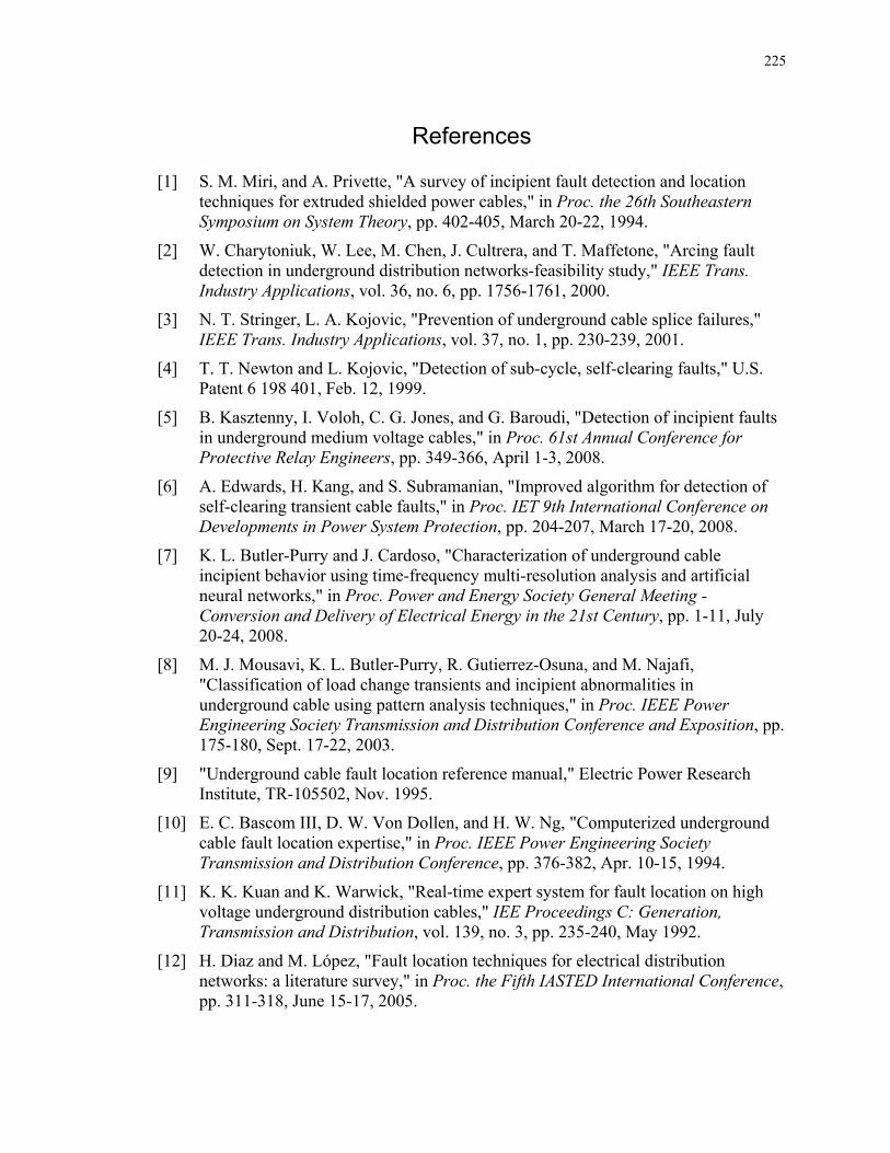
225
References
[1] S. M. Miri, and A. Privette, "A survey of incipient fault detection and location techniques for extruded shielded power cables," in Proc. the 26th Southeastern Symposium on System Theory, pp. 402-405, March 20-22, 1994.
[2] W. Charytoniuk, W. Lee, M. Chen, J. Cultrera, and T. Maffetone, "Arcing fault detection in underground distribution networks-feasibility study," IEEE Trans. Industry Applications, vol. 36, no. 6, pp. 1756-1761, 2000.
[3] N. T. Stringer, L. A. Kojovic, "Prevention of underground cable splice failures," IEEE Trans. Industry Applications, vol. 37, no. 1, pp. 230-239, 2001.
[4] T. T. Newton and L. Kojovic, "Detection of sub-cycle, self-clearing faults," U.S. Patent 6 198 401, Feb. 12, 1999.
[5] B. Kasztenny, I. Voloh, C. G. Jones, and G. Baroudi, "Detection of incipient faults in underground medium voltage cables," in Proc. 61st Annual Conference for Protective Relay Engineers, pp. 349-366, April 1-3, 2008.
[6] A. Edwards, H. Kang, and S. Subramanian, "Improved algorithm for detection of self-clearing transient cable faults," in Proc. IET 9th International Conference on Developments in Power System Protection, pp. 204-207, March 17-20, 2008.
[7] K. L. Butler-Purry and J. Cardoso, "Characterization of underground cable incipient behavior using time-frequency multi-resolution analysis and artificial neural networks," in Proc. Power and Energy Society General Meeting - Conversion and Delivery of Electrical Energy in the 21st Century, pp. 1-11, July 20-24, 2008.
[8] M. J. Mousavi, K. L. Butler-Purry, R. Gutierrez-Osuna, and M. Najafi, "Classification of load change transients and incipient abnormalities in underground cable using pattern analysis techniques," in Proc. IEEE Power Engineering Society Transmission and Distribution Conference and Exposition, pp. 175-180, Sept. 17-22, 2003.
[9] "Underground cable fault location reference manual," Electric Power Research Institute, TR-105502, Nov. 1995.
[10] E. C. Bascom III, D. W. Von Dollen, and H. W. Ng, "Computerized underground cable fault location expertise," in Proc. IEEE Power Engineering Society Transmission and Distribution Conference, pp. 376-382, Apr. 10-15, 1994.
[11] K. K. Kuan and K. Warwick, "Real-time expert system for fault location on high voltage underground distribution cables," IEE Proceedings C: Generation, Transmission and Distribution, vol. 139, no. 3, pp. 235-240, May 1992.
[12] H. Diaz and M. López, "Fault location techniques for electrical distribution networks: a literature survey," in Proc. the Fifth IASTED International Conference, pp. 311-318, June 15-17, 2005.
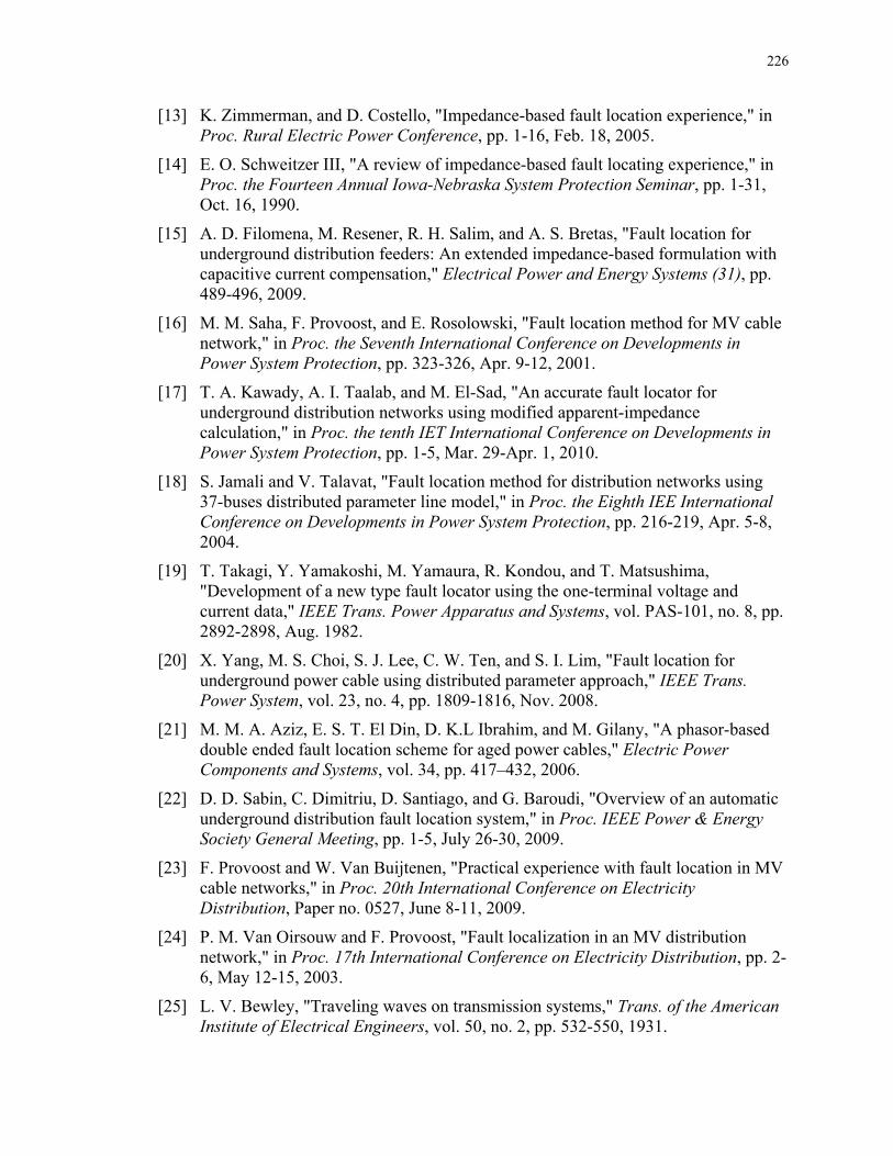
226
[13] K. Zimmerman, and D. Costello, "Impedance-based fault location experience," in Proc. Rural Electric Power Conference, pp. 1-16, Feb. 18, 2005.
[14] E. O. Schweitzer III, "A review of impedance-based fault locating experience," in Proc. the Fourteen Annual Iowa-Nebraska System Protection Seminar, pp. 1-31, Oct. 16, 1990.
[15] A. D. Filomena, M. Resener, R. H. Salim, and A. S. Bretas, "Fault location for underground distribution feeders: An extended impedance-based formulation with capacitive current compensation," Electrical Power and Energy Systems (31), pp. 489-496, 2009.
[16] M. M. Saha, F. Provoost, and E. Rosolowski, "Fault location method for MV cable network," in Proc. the Seventh International Conference on Developments in Power System Protection, pp. 323-326, Apr. 9-12, 2001.
[17] T. A. Kawady, A. I. Taalab, and M. El-Sad, "An accurate fault locator for underground distribution networks using modified apparent-impedance calculation," in Proc. the tenth IET International Conference on Developments in Power System Protection, pp. 1-5, Mar. 29-Apr. 1, 2010.
[18] S. Jamali and V. Talavat, "Fault location method for distribution networks using 37-buses distributed parameter line model," in Proc. the Eighth IEE International Conference on Developments in Power System Protection, pp. 216-219, Apr. 5-8, 2004.
[19] T. Takagi, Y. Yamakoshi, M. Yamaura, R. Kondou, and T. Matsushima, "Development of a new type fault locator using the one-terminal voltage and current data," IEEE Trans. Power Apparatus and Systems, vol. PAS-101, no. 8, pp. 2892-2898, Aug. 1982.
[20] X. Yang, M. S. Choi, S. J. Lee, C. W. Ten, and S. I. Lim, "Fault location for underground power cable using distributed parameter approach," IEEE Trans. Power System, vol. 23, no. 4, pp. 1809-1816, Nov. 2008.
[21] M. M. A. Aziz, E. S. T. El Din, D. K.L Ibrahim, and M. Gilany, "A phasor-based double ended fault location scheme for aged power cables," Electric Power Components and Systems, vol. 34, pp. 417–432, 2006.
[22] D. D. Sabin, C. Dimitriu, D. Santiago, and G. Baroudi, "Overview of an automatic underground distribution fault location system," in Proc. IEEE Power & Energy Society General Meeting, pp. 1-5, July 26-30, 2009.
[23] F. Provoost and W. Van Buijtenen, "Practical experience with fault location in MV cable networks," in Proc. 20th International Conference on Electricity Distribution, Paper no. 0527, June 8-11, 2009.
[24] P. M. Van Oirsouw and F. Provoost, "Fault localization in an MV distribution network," in Proc. 17th International Conference on Electricity Distribution, pp. 2-6, May 12-15, 2003.
[25] L. V. Bewley, "Traveling waves on transmission systems," Trans. of the American Institute of Electrical Engineers, vol. 50, no. 2, pp. 532-550, 1931.
227
[26] P. F. Gale, P. A. Crossley, B. Xu, Y. Ge, B. J. Cory, and J. R. G. Barker, "Fault location based on travelling waves," in Proc. Fifth International Conference on Developments in Power System Protection, pp. 54-59, Mar. 30-Apr. 1, 1993.
[27] Z. Q. Bo, R. K. Aggarwal, A. T. Johns, and P. J. Moore, "Accurate fault location and protection scheme for power cable using fault generated high frequency voltage transients," in Proc. the Eight Mediterranean Electro-technical Conference, Industrial Applications in Power Systems, pp. 777-780, May 1996.
[28] Z. Chen, Z. Q. Bo, F. Jiang, X. Z. Dong, G. Weller, and N. F. Chin, "Wavelet transform based accurate fault location and protection technique for cable circuits," in Proc. International Conference on Advances in Power System Control, Operation and Management, pp. 59-63, Oct. 30-Nov. 1, 2000.
[29] W. Zhao, Y. H. Song, and W. R. Chen, "Improved GPS travelling wave fault locator for power cables by using wavelet analysis," Electrical Power System Research (23), pp. 403-411, 2001.
[30] M. Gilany, D. Ibrahim, and E. S. Tag Eldin, "Traveling-wave-based fault-location scheme for multiend-aged underground cable system," IEEE Trans. Power Delivery, vol. 22, no. 1, pp. 82-89, Jan. 2010.
[31] H. Hizam, P. A. Crossley, P. F. Gale, and G. Bryson, "Fault section identification and location on a distribution feeder using travelling waves," in Proc. IEEE Power & Energy Society Summer Meeting, vol. 3, pp. 1107-1112, July 25, 2002.
[32] J. Sadeh and H. Afradi, "A new and accurate fault location algorithm for combined transmission lines using adaptive network-based fuzzy inference system," Electrical Power System Research (79), pp. 1538-1545, 2009.
[33] J. Moshtagh and R. K. Aggarwal, "A new approach to ungrounded fault location in a three-phase underground distribution system using combined neural networks & wavelet analysis," in Proc. Canadian Conference on Electrical and Computer Engineering, pp. 376-381, May 2006.
[34] "Distribution Fault Location," Electric Power Research Institute, 1012438, Dec. 2006.
[35] IEEE Guide for Determining Fault Location on AC Transmission and Distribution Lines, IEEE Standard C37.114-2004, June 2005.
[36] J. Mora-Flòrez, J. Meléndez, and G. Carrillo-Caicedo, "Comparison of impedance based fault location methods for power distribution systems," Electrical Power System Research (78), pp. 657-666, 2008.
[37] T. Short, J. Kim, and C. Melhorn, "Update on distribution system fault location technologies and effectiveness," in Proc. 20th International Conference and Exhibition on Electricity Distribution - Part 1, paper no. 0973, June 8-11, 2009.
[38] M. Lehtonen, "Novel techniques for fault location in distribution networks," in Proc. Power Quality and Supply Reliability Conference, pp. 1-6, Aug. 27-29, 2008.
228
[39] K. Srinivasan and A. St.-Jacques, "A new fault location algorithm for radial transmission lines with loads," IEEE Trans. Power Delivery, vol. 4, no. 3, pp. 1676-1682, July 1989.
[40] A. A. Girgis, C. M. Fallon, and D. L. Lubkeman, "A fault location technique for rural distribution feeders," IEEE Trans. Industry Application, vol. 29, no. 6, pp. 1170-1175, Nov. 1993.
[41] J. Zhu, D. L. Lubkeman, and A. A. Girgis, "Automated fault location and diagnosis on electric power distribution feeders," IEEE Trans. on Power Delivery, vol. 12, no. 2, pp. 801-809, April 1997.
[42] R. Aggarwal, Y. Aslan, and A. Johns, "New concept in fault location for overhead distribution systems using superimposed components," IEE Proc. Generation, Transmission and Distribution, vol. 144, no. 3, pp. 309-316, May 1997.
[43] Y. Aslan and R. K. Aggarwal, "An alternative approach to fault location on main line feeders and laterals in low voltage overhead distribution networks," in Proc. IET 9th International Conference on Developments in Power System Protection, pp. 354-359, mar. 17-20, 2008.
[44] R. Das, "Determining the locations of faults in distribution systems," Ph.D. thesis, Dept. Elec. Eng., Univ. Saskatchewan, 1998.
[45] R. Das, M.S. Sachdev, and T. S. Sidhu, "A fault locator for radial subtransmission and distribution lines," in Proc. IEEE Power & Energy Society Summer Meeting, vol. 1, pp. 443-448, 2000.
[46] D. Novosel, D. Hart, Y. Hu, and J. Myllymaki, "System for locating faults and estimating fault resistance in distribution networks with tapped loads," U.S. Patent 5 839 093, Nov. 17, 1998.
[47] S. Santoso, R. C. Dugan, J. Lamoree, and A. Sundaram, "Distance estimation technique for single line-to-ground faults in a radial distribution system," in Proc. IEEE Power & Energy Society Winter Meeting, pp. 2551-2555, Jan. 23-27, 2000.
[48] M. Saha and E. Rosolowski, "Method and device of fault location for distribution networks," U.S. Patent 6 483 435, Nov. 19, 2002.
[49] M. Saha, E. Rosolowski, and J. Izykowski, "ATP-EMTP investigation for fault location in medium voltage networks," in Proc. International Conference on Power Systems Transients, paper no. IPST05-220, June 19-23, 2005.
[50] S.-J. Lee, M.-S. Choi, S.-H. Kang, B.-G. Jin, D.-S. Lee, B.-S. Ahn, N.-S. Yoon, H.-Y. Kim, and S.-B. Wee, "An intelligent and efficient fault location and diagnosis scheme for radial distribution systems, " IEEE Trans. Power Delivery, vol. 19, no. 2, pp. 524–532, Apr. 2004.
[51] E. C. Senger, G. Jr. Manassero, C. Goldemberg, and E. L. Pellini, "Automated fault location system for primary distribution networks," IEEE Trans. Power Delivery, vol. 20, no. 2, pp. 1332-1340, April 2005.
229
[52] R. H. Salim, M. Resener, A. D. Filomena, K. R. C. de Oliveira, and A. S. Bretas, "Extended fault-location formulation for power distribution systems," IEEE Trans. Power Delivery, vol. 24, no. 2, pp. 508-516, April 2009.
[53] R. A. F. Pereira, L. G. W. da Silva, M. Kezunovic, and J. R. S. Mantovani, "Improved fault location on distribution feeders based on matching during-fault voltage sags," IEEE Trans. Power Delivery, vol. 24, no. 2, pp. 852-866, April 2009.
[54] G. Morales-Espana, J. Mora-Florez, and H. Vargas-Torres, "Elimination of multiple estimation for fault location in radial power systems by using fundamental single-end measurements," IEEE Trans. Power Delivery, vol. 24, no. 3, pp. 1382-1389, July 2009.
[55] M. M. Alamuti, H. Nouri, N. Makhol, and M. Montakhab, "Developed single end low voltage fault location using distributed parameter approach," in Proc. the 44th International Universities Power Engineering Conference, pp. 1-5, Sept. 1-4, 2009.
[56] M. A. Mirzai and A. A. Afzalian, "A novel fault-locator system; algorithm, principle and practical implementation," IEEE Trans. on Power Delivery, vol. 25, no. 1, pp. 35-46, Jan. 2010.
[57] Y. Liao, "Generalized fault-location methods for overhead electric distribution systems," IEEE Trans. on Power Delivery, vol. 26, no. 1, pp. 53-64, Jan. 2011.
[58] W. H. Kersting, Distribution System Modeling and Analysis. Boca Ratón, FL: CRC, 2002.
[59] C. S. Cheng and D. Shirmohammadi, “A three-phase power flow method for real-time distribution system analysis,” IEEE Trans. Power System, vol. 10, no. 2, pp. 671–679, May 1995.
[60] W. H. Kersting and W. H. Phillips, "Distribution feeder line models," IEEE Trans. Industry Applications, vol. 31, no. 4, pp. 715-720, July/Aug. 1995.
[61] J. J. Grainger and W. D. Stevenson Jr., Power system analysis, New York: McGraw-Hill, 1994.
[62] K. Srinivasan, C. T. Nguyen, Y. Robichaud, A. St. Jacques, and G. J. Rogers, "Load response coefficients monitoring system: Theory and field experience," IEEE Trans. Power Apparatus and Systems, vol. PAS-100, no. 8, pp. 3818-3827, Aug. 1981.
[63] C. A. Reineri and C Alvarez, "Load research for fault location in distribution feeders," IEE Proc. Generation, Transmission and Distribution, vol. 146, no. 2, pp. 115-120, May 1999.
[64] J. Wan, "Nodal load estimation for electric power distribution systems," Ph.D. thesis, Dept. Elec. Eng., Drexel Univ., 2003.
[65] J. Wan and K. N. Miu, "Weighted least squares methods for load estimation in distribution networks," IEEE Trans. Power System, vol. 18, no. 4, pp. 1338-1345, Nov. 2003.
230
[66] M. Baran and A. W. Kelley, "State estimation for real time monitoring of distribution systems," IEEE Trans. Power System, vol. 9, no. 3, pp. 1601-1609, Aug. 1994.
[67] M. E. Baran and A. W. Kelley, "A branch-current-based state estimation method for distribution systems" IEEE Trans. Power System, vol. 10, no. 1, pp. 483-491, Feb. 1995.
[68] W.-M. Lin, J.-H. Teng, and S.-J. Chen, "A highly efficient algorithm in treating current measurements for the branch-current-based distribution state estimation," IEEE Trans. Power Delivery, vol. 16, no. 3, pp. 433-439, July 2001.
[69] M. R. Irving and C. N. Macqueen, "Robust algorithm for load estimation in distribution networks," IEE Proc. Generation, Transmission and Distribution, vol. 145, no. 5, pp. 499-504, Sept. 1998.
[70] M. K. Celik and W. H. E. Liu, "A practical distribution state calculation algorithm," in Proc. IEEE Power & Energy Society Winter Meeting, vol. 1, pp. 442-447, 1999.
[71] A. Gomez Esposito and E. Romero Ramos, "Reliable load flow technique for radial distribution networks," IEEE Trans. Power System, vol. 14, no. 3, pp. 1063-1069, Aug. 1999.
[72] J.-H. Teng and C.-Y. Chang, "A novel and fast three-phase load flow for unbalanced radial distribution systems" IEEE Trans. Power System, vol. 17, no. 4, pp. 1238-1244, Nov. 2002.
[73] R. A. Jabr, "Radial distribution load flow using conic programming," IEEE Trans. Power System, vol. 21, no. 3, pp. 1458-1459, Aug. 2006.
[74] R. Ross, "Inception and propagation mechanisms of water treeing," IEEE Trans. Dielectrics and Electrical Insulation, vol. 5, no. 5, pp. 660-680, Oct. 1998.
[75] G. Chen and C. H. Tham, "Electrical treeing characteristics in XLPE power cable insulation in frequency range between 20 and 500 Hz," IEEE Trans. Dielectrics and Electrical Insulation, vol. 16, no. 1, pp. 179-188, Feb. 2009.
[76] M. S. Mashikian and A. Szatkowski, "Medium voltage cable defects revealed by off-line partial discharge testing at power frequency," IEEE Electrical Insulation Magazine, vol. 22, no. 4, pp. 24-32, July/Aug. 2006.
[77] J. Densley, "Ageing mechanisms and diagnostics for power cables - an overview," IEEE Electrical Insulation Magazine, vol. 17, no. 1, pp. 14-22, Jan./Feb. 2001.
[78] B. Koch, and Y. Carpentier, "Manhole explosion due to arcing faults on underground secondary distribution cables in ducts," IEEE Trans. Power Delivery, vol. 7, no. 3, pp. 1425-1433, July 1992.
[79] A. Hamel, A. Gaudreau, and M. Côté, "Intermittent arcing fault on underground low-voltage cables," IEEE Trans. Power Delivery, vol. 19, no. 4, pp. 1862-1868, Oct. 2004.
[80] IEEE Guide for Performing Arc-Flash Hazard Calculations, IEEE Standard 1584-2002.
231
[81] R. Wilkins, M. Allison, and M. Lang, "Improved method for arc flash hazard analysis – calculating hazards," IEEE Ind. Application Magazine, vol. 11, no. 3, pp. 40–48, 2005.
[82] T. Gammon and J. Matthews, "The historical evolution of arcing-fault models for low-voltage systems," in Proc. Industrial and Commercial Power Systems Technical Conference, pp. 1-6, Aug. 1999.
[83] H. A. Darwish and N. I. Elkalashy, "Universal arc representation using EMTP," IEEE Trans. Power Delivery, vol. 20, no. 2, pp. 772–779, Apr. 2000.
[84] U. Habedank, "Application of a new arc model for the evaluation of short-circuit breaking tests," IEEE Trans. Power Delivery, vol. 8, no. 4, pp. 1921–1925, Oct. 1993.
[85] M. Kizilcay, and P. La Seta, "Digital simulation of fault arcs in medium-voltage distribution networks," in Proc. 15th Power Systems Computation Conference, session 36, paper 3, pp. 1-7, August 22-26, 2005.
[86] G. I. Ospina, D. Cubillos, and L. Ibanez, "Analysis of arcing fault models," in Proc. IEEE Power Engineering Society Transmission and Distribution Conference and Exposition: Latin America, pp. 1-5, Aug. 13-15, 2008
[87] D.C. Robertson, O.I. Camps, J.S. Mayer, and W.B. Gish, "Wavelets and electromagnetic power system transients," IEEE Trans. Power Delivery, vol. 11, no. 2, pp. 1050-1058, Apr. 1996.
[88] N.S.D. Brito, B.A. Souza, and F.A.C. Pires, "Daubechies wavelets in quality of electrical power," in Proc. 8th International Conference on Harmonics and Quality of Power, pp. 511-515, Oct 14-16, 1998.
[89] I. Daubechies, Ten Lectures on Wavelets, SIAM, 1992.
[90] A. V. Oppenheim, R.W. Schafer, and J. R. Buck, Discrete-time signal processing, 2nd ed., Prentice-Hall, 1998.
[91] IEEE Standard Common Format for Transient Data Exchange (COMTRADE) for Power Systems, IEEE Std. 37.111-1991.
[92] W.H. Kersting, "Radial distribution test feeders," in Proc. IEEE Power & Energy Society Winter Meeting, vol. 2, pp. 908-912, Jan. 28-Feb. 1, 2001.
[93] B. Gustavsen, "Panel session on data for modeling system transients insulated cables," in Proc. IEEE Power & Energy Society Winter Meeting, vol. 2, pp. 718-723, Jan. 28-Feb. 1, 2001.
[94] IEEE Guide for Application of Sheath-Bonding Methods for Single-Conductor Cables and the Calculation of Induced Voltages and Currents in Cable Sheaths, IEEE Standard 575-988, March 1986.
[95] D. A. Tziouvaras, "Protection of high-voltage AC cables," in Proc. Power Systems Conference: Advanced Metering, Protection, Control, Communication and Distributed Resources, pp 316-328, Mar. 14-17, 2006.
232
[96] J. Zipp, "Protective relaying considerations for transmission lines with high voltage AC cables," IEEE Trans. on Power Delivery, vol. 12, no. 1, pp. 83-96, Jan. 1997.
[97] B. Kasztenny, I. Voloh, and J. G. Hubertus, "Applying distance protection to cable circuits," in Proc. 57th Annual Conference for Protective Relay Engineers, pp. 46-69, Mar. 30-Apr. 1, 2004.
[98] V. Leitloff, X. Bourgeat, and G. Duboc, "Setting constraints for distance protection on underground lines," in Proc. Seventh International Conference on Developments in Power System Protection, pp. 467-470, Apr. 9-12, 2001.
[99] J. Vargas, A. Guzmán, and J. Robles, "Underground/submarine cable protection using a negative-sequence directional comparison scheme," [Online]. Available: www2.selinc.com/techpprs/underground.pdf.
[100] C. L. Fortescue, "Method of symmetrical co-ordinates applied to the solution of polyphase networks," Trans. of American Institute of Electrical Engineers, vol. XXXVII, no. 2, pp. 1027-1140, July, 1918.
[101] E. Clarke, Circuit Analysis of AC Power Systems, vol. I. New York: Wiley, 1950.
[102] J. A. Brandao Faria and J. H. Briceno Mendez, "Modal analysis of untransposed bilateral three-phase lines - a perturbation approach," IEEE Trans. on Power Delivery, vol. 12, no. 1, pp. 497-504, Jan. 1997.
[103] A. J. do Prado, J. P. Filho, S. Kurokawa, and E. F. Bovolato, "Correction procedure applied to a single real transformation matrix -untransposed three-phase transmission line cases," in Proc. IEEE Power Engineering Society Transmission & Distribution Conference and Exposition: Latin America, pp. 1-6, Aug. 15-18, 2006.
[104] G. Kron, Tensor analysis of networks, New York: Wiley, 1939.
[105] L. Marti, "Simulation of electromagnetic transients in underground cables using the EMTP," in Proc. the 2nd International Conference on Advances in Power System Control, Operation and Management, pp. 147-152, Dec. 7-10, 1993.
[106] L. Marti, "Simulation of transients in underground cables with frequency-dependent modal transformation matrices," IEEE Trans. on Power Delivery, vol. 3, no. 3, pp. 1099-1110, July 1988.
[107] "PSCAD/EMTDC User’s Guide," Manitoba HVDC Research Center, 2004.
[108] J. R. Carson, "Wave propagation in overhead wires with ground return," Bell System Technical Journal, vol. 5, pp. 539-554, 1926.
[109] L. M. Wedepohl and D. J. Wilcox, "Transient analysis of underground power-transmission systems. System-model and wave-propagation characteristics," Proceedings of the Institution of Electrical Engineers, vol. 120, no. 2, pp. 253-260, Feb. 1973.
[110] G. C. Stone and S. A. Boggs, "Propagation of partial discharge pulses in shielded power cable," in Proc. Annual Report of the Conference on Electrical Insulation and Dielectric Phenomena, pp. 275–280, 1982.

233
[111] The Mathworks, Inc., Mathworks Matlab [Online]. Available: http://www.mathworks.com.
[112] M. E. Baran, "Challenges in state estimation on distribution systems," in Proc. IEEE Power & Energy Society Summer Meeting, vol. 1, pp. 429-433, 2001.
[113] J. F. Bonnans, J. C. Gilbert, C. Lemarechal, and C. A. Sagastizábal, Numerical optimization: Theoretical and practical aspects, 2nd ed., New York: Springer, 2006.
[114] A. Antoniou and W.-S. Lu, Practical optimization algorithms and engineering applications, New York: Springer, 2007.
[115] J. C. Gilbert, SQPlab: A Matlab software for solving nonlinear optimization problems and optimal control problems. [Online]. Available: http://www-rocq.inria.fr/~gilbert/preprint/u02-sqplab.pdf.
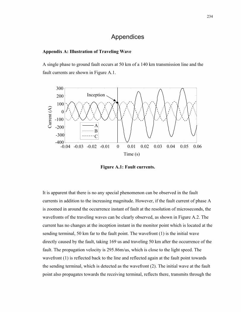
234
Appendices
Appendix A: Illustration of Traveling Wave
A single phase to ground fault occurs at 50 km of a 140 km transmission line and the
fault currents are shown in Figure A.1.
Figure A.1: Fault currents.
It is apparent that there is no any special phenomenon can be observed in the fault
currents in addition to the increasing magnitude. However, if the fault current of phase A
is zoomed in around the occurrence instant of fault at the resolution of microseconds, the
wavefronts of the traveling waves can be clearly observed, as shown in Figure A.2. The
current has no changes at the inception instant in the monitor point which is located at the
sending terminal, 50 km far to the fault point. The wavefront (1) is the initial wave
directly caused by the fault, taking 169 us and traveling 50 km after the occurrence of the
fault. The propagation velocity is 295.86m/us, which is close to the light speed. The
wavefront (1) is reflected back to the line and reflected again at the fault point towards
the sending terminal, which is detected as the wavefront (2). The initial wave at the fault
point also propagates towards the receiving terminal, reflects there, transmits through the
-0.04 -0.03 -0.02 -0.01 0 0.01 0.02 0.03 0.04 0.05 0.06-400
-300
-200
-100
0
100
200
300
Time (s)
ABC
Cur
rent
(A
)
Inception
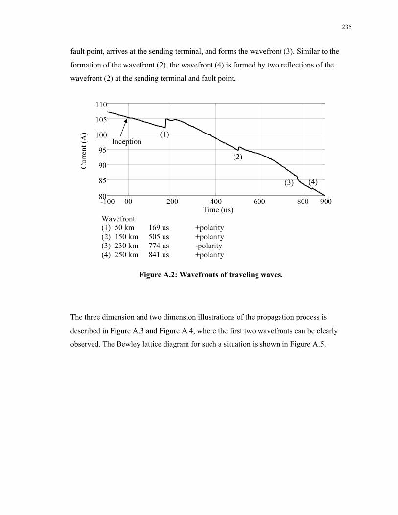
235
fault point, arrives at the sending terminal, and forms the wavefront (3). Similar to the
formation of the wavefront (2), the wavefront (4) is formed by two reflections of the
wavefront (2) at the sending terminal and fault point.
Figure A.2: Wavefronts of traveling waves.
The three dimension and two dimension illustrations of the propagation process is
described in Figure A.3 and Figure A.4, where the first two wavefronts can be clearly
observed. The Bewley lattice diagram for such a situation is shown in Figure A.5.
-100 00 200 400 600 800 90080
85
90
95
100
105
110
Time (us)
Inception
Wavefront (1) 50 km 169 us +polarity (2) 150 km 505 us +polarity (3) 230 km 774 us -polarity (4) 250 km 841 us +polarity
(1)
(2)
(3) (4)
Cur
rent
(A
)
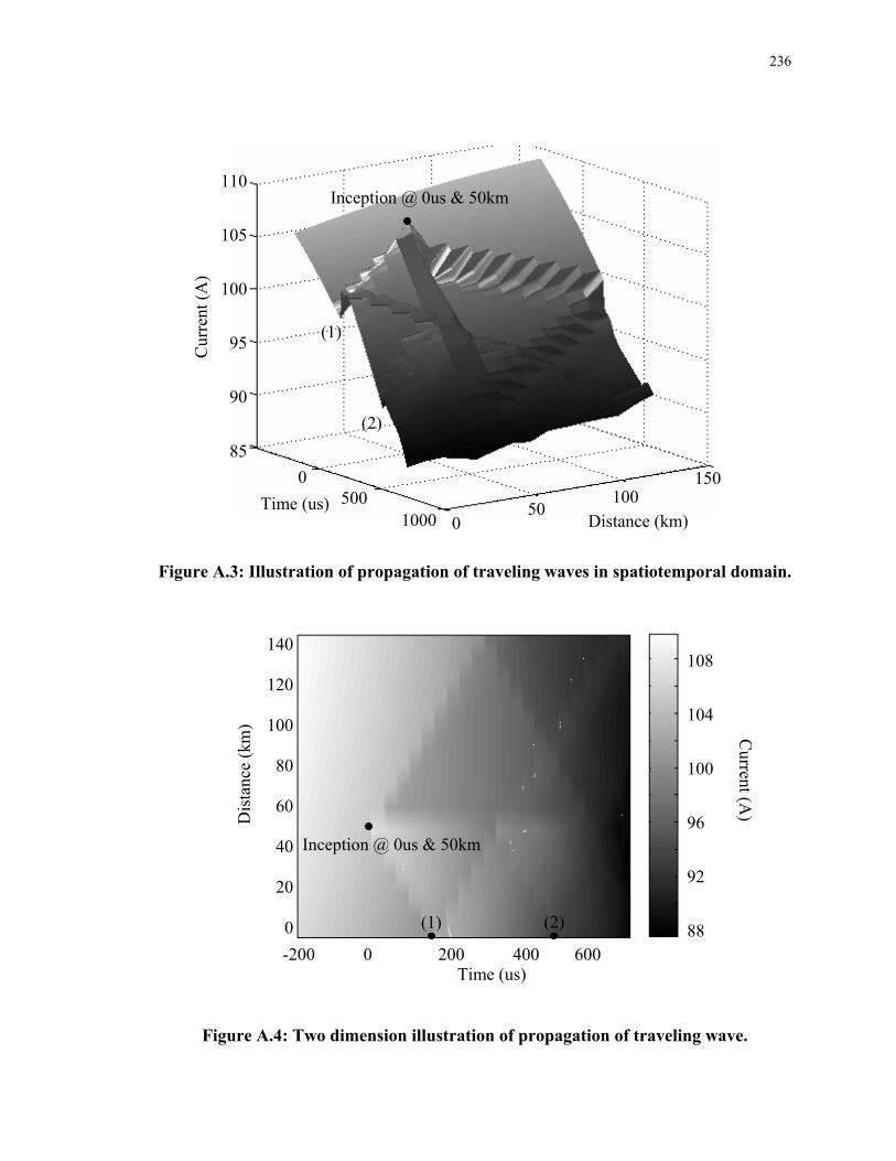
236
Figure A.3: Illustration of propagation of traveling waves in spatiotemporal domain.
Figure A.4: Two dimension illustration of propagation of traveling wave.
140
120
100
80
60
40
20
0
-200 0 200 400 600
108
104
100
96
92
88
Time (us)
Inception @ 0us & 50km
Dis
tanc
e (k
m)
(1) (2)
Current (A
)
110
105
100
95
90
85
0 500
1000 0 50
100 150
Time (us) Distance (km)
Cur
rent
(A
)
(1)
(2)
Inception @ 0us & 50km
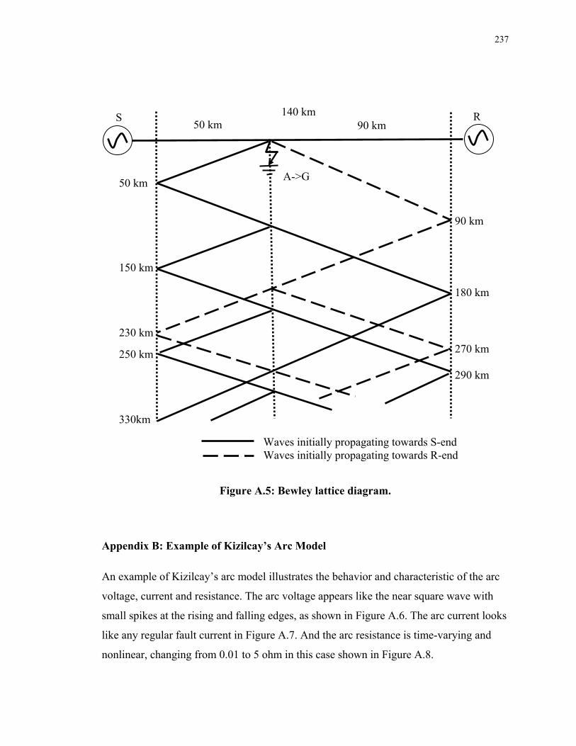
237
Figure A.5: Bewley lattice diagram.
Appendix B: Example of Kizilcay’s Arc Model
An example of Kizilcay’s arc model illustrates the behavior and characteristic of the arc
voltage, current and resistance. The arc voltage appears like the near square wave with
small spikes at the rising and falling edges, as shown in Figure A.6. The arc current looks
like any regular fault current in Figure A.7. And the arc resistance is time-varying and
nonlinear, changing from 0.01 to 5 ohm in this case shown in Figure A.8.
140 km50 km
A->G 50 km 150 km 230 km
250 km 330km
90 km 180 km 270 km 290 km
S R90 km
Waves initially propagating towards S-end Waves initially propagating towards R-end
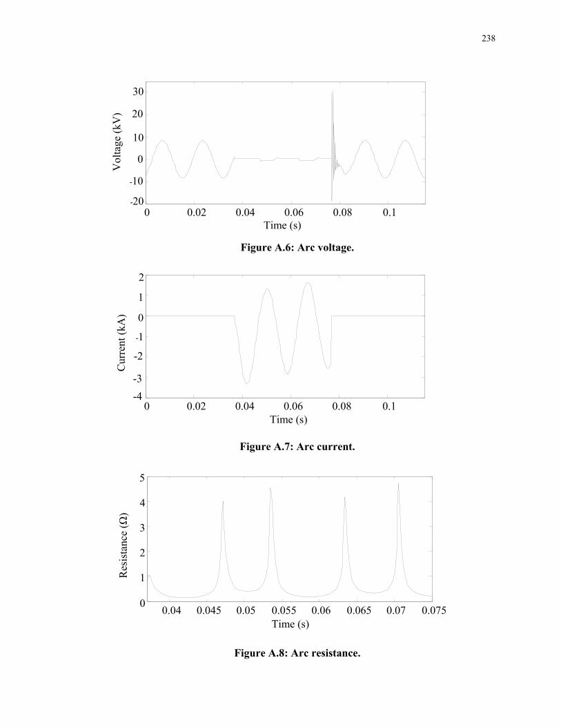
238
Figure A.6: Arc voltage.
Figure A.7: Arc current.
Figure A.8: Arc resistance.
0 0.02 0.04 0.06 0.08 0.1 -20
-10
0
10
20
30
Time (s)
Vol
tage
(kV
)
0 0.02 0.04 0.06 0.08 0.1 -4
-3
-2
-1
0
1
2
Time (s)
Cur
rent
(kA
)
0.04 0.045 0.05 0.055 0.06 0.065 0.07 0.075 0
1
2
3
4
5
Time (s)
Res
ista
nce
(Ω)

239
Curriculum Vitae
Name: Zhihan Xu Post-secondary Sichuan University Education and Chengdu, Sichuan, China Degrees: 1991-1995 B.E.
Sichuan University Chengdu, Sichuan, China 1997-2000 M.Sc.
The University of Alberta Edmonton, Alberta, Canada 2000-2002 M.Sc.
The University of Western Ontario London, Ontario, Canada 2007-2011 Ph.D.
Honors and Western Graduate Research Scholarship - Engineering Awards: 2007-2011 Related Work Research Assistant and Teaching Assistant Experience The University of Western Ontario
2007-2011 Publications: T. S. Sidhu and Z. Xu, “Detection and Classification of Incipient Faults in Underground Cables in Distribution Systems”, in Proc. Canadian Conference on Electrical and Computer Engineering, pp. 122-126, May 3-6, 2009. T. S. Sidhu and Z. Xu, "Detection of incipient faults in distribution underground cables," IEEE Trans. Power Del., vol. 25, no. 3, pp. 1363-1371, July 2010. Z. Xu and T. S. Sidhu, "Fault location method based on single-end measurements for underground cables," IEEE Trans. Power Del., vol. 26, no. 4, pp. 2845-2854, October 2011. Z. Xu and T. S. Sidhu, "Fault location for cables in distribution networks with the aid of state estimation," to be submitted.
Related Documents