Fault Detection and Isolation for Linear Dynamical Systems · Fault Detection and Isolation for Linear Dynamical Systems ... com aplicação na área de deteção e isolamento de

Fault Detection and Isolation for Linear Dynamical Systems

Diogo Filipe Guerreiro Piçarra da Cunha Monteiro

Thesis to obtain the Master of Science Degree in

Aerospace Engineering

Supervisors: Prof. Paulo Jorge Coelho Ramalho OliveiraProf. Carlos Jorge Ferreira Silvestre

Expert: Doctor Paulo André Nobre Rosa

Examination Committee

Chairperson: Professor João Manuel Lage de Miranda LemosSupervisor: Prof. Paulo Jorge Coelho Ramalho Oliveira

Member of the Committee: Professor João Miguel da Costa Sousa

October 2015

ii

To my parents.

iii

iv

Acknowledgements

I would like to start by showing my gratitude to my co-supervisor, Prof. Paulo Oliveira, for his guid-

ance and support throughout this thesis. His deep knowledge and experience certainly contributed to

develop my research and to obtain a more consolidated work. Also, the high standards he requires from

his students led me to be more exigent with my work and constantly search for improvement. Not least

important, I would like to address my gratitude to Prof. Carlos Silvestre, that despite supervising me

from Macau, always made his important opinion clear through Prof. Paulo Oliveira.

My next gratitude words go to my thesis advisor Dr. Paulo Rosa for his unconditional support in

providing determinant recommendations and advices during the last six months. Certainly, his expertise

and incredible intuition were fundamental to find the right research path. Through his person, I shall

also thank Deimos Engenharia, S.A. and everyone there that always received me with enthusiasm and

provided everything I required to develop my work there.

I would like to thank the Institute for Systems and Robotics (ISR) and all my colleagues there, that

through countless conversations and lunches together helped me to solve several problems during my

research. Also, their support, encouragement, and enthusiasm were paramount during this stage of my

academic path.

I can not finish without a very special gratitude word to two incredible student groups in Técnico.

To the Autonomous Section of Applied Aeronautics (S3A) for enabling me to develop deeply interesting

hands-on projects during my course and to collaborate with an enthusiastic group of colleagues, that

share the same passion for aviation. The second group is the Técnico’s Football team in which I took

part during the last 4 years. There, I came across the most incredible human beings that today I call

friends. For their encouragement and great advice during every moment we shared, and for everything

I learned by participating in this team, I address my deepest thankfulness.

I’m also thankful to my closest friends. They were unconditionally present every time I needed and

with them I shared some of the most important moments during my years at the University. A special

thanks to João for the patience of revising this thesis.

Finally, my utmost gratitude words go to all my family but particularly to my parents, Ana Paula and

Filipe, my sisters, Rafaela and Ana Filipe, and my grandparents for their endless support and advice

during these years, and to Ana, for her love and unconditional friendship.

v

vi

Resumo

A Segurança e fiabilidade de sistemas dinâmicos é um problema que tem acompanhado o desen-

volvimento da tecnologia tanto na comunidade científica, como também na indústria. A importância de

monitorizar a condição de um sistema é, ainda mais, relevante para sistemas críticos, como na indústria

química e nuclear, medicina, transportes e sistemas de segurança. A ocorrência de eventos atípicos

nestes processos pode levar à deterioração da operação, ou até mesmo a catástrofes quando as falhas

são significativas. A relevância deste tema e também o crescente interesse por técnicas de múltiplos

modelos, com aplicação na área de deteção e isolamento de falhas em tempo-real, motiva o desen-

volvimento desta tese.

Inicialmente, aborda-se a técnica clássica de estimação adaptativa com múltiplos modelos (MMAE),

através de um estudo aprofundado para o desenho de uma arquitetura capaz de determinação do

regime de funcionamento de um sistema. Isto é atingido através da identificação da região em que os

parâmetros da falha estão localizados, tendo em conta o domínio de incerteza associado. Este pro-

cesso decorre de uma estratégia baseada na avaliação da performance de estimação dos estados, que

deverá ser independente da localização dos parâmetros da falha.

Devido à elevada exigência computacional do sistema MMAE clássico, de seguida propõe-se um

novo desenho para o banco de estimadores através da combinação de filtros de Kalman e filtros H2

robustos. A estratégia desenvolvida leva a uma redução substancial no número de filtros presentes no

banco, e simultaneamente mantém o nível de performance de estimação pretendido.

Em ambas as propostas as propriedades de convergência assimptótica são avaliadas, de forma a

garantir a robustez dos métodos. Utilizando um modelo dinâmico genérico de um helicóptero, várias

simulações computacionais são executadas de forma a provar o potencial dos métodos desenvolvidos

e também fornecer uma base de verificação dos resultados teóricos alcançados.

Palavras-chave: estimação adaptativa com múltiplos modelos; diagnóstico de falhas com base

em modelos dinâmicos; filtros H2 robustos; estimação de estados em regime de incerteza;

vii

viii

Abstract

Safety and reliability of a dynamical system is a concern that have always pursued designers in both

academia and industry. Monitoring the health status of a system is even more relevant for safety critical

applications, such as chemical and nuclear plants, medicine, transportation, and security systems. The

occurrence of abnormal events on these processes may lead to malfunctions and disasters in ultimate

fault conditions, as witnessed in the past. The paramount importance of the topic and the increasing

interest in multiple-model approaches under the scope of on-line fault detection and isolation motivates

this thesis.

Initially, focus is given to classical multiple-model adaptive estimation (MMAE) in which an in-depth

study is undertaken for the design of a scheme capable of determining the working regime of a system.

This is done by identifying the region where the fault parameters lie under the associated uncertainty

domain. The design procedure is built on a performance-based strategy, which ensures a well-defined

level of state estimation performance despite the fault location.

Due to the high computational complexity of the classical MMAE approach, in what follows we pro-

pose a novel bank design based on the combination of Kalman and robustH2 filters. This strategy leads

to a substantial reduction on the number of estimators in the bank, while preserving the desired state

estimation performance.

In both approaches a prominent study on convergence properties is performed, so that robustness

of the methods is guaranteed. Computational simulations based on a generic helicopter model are

also executed to prove the potential of the strategies developed and provide a verification basis for the

theoretical results achieved.

Keywords: Multiple-model adaptive estimation; model-based fault diagnosis; robust H2 filters;

state estimation in uncertain systems;

ix

x

Contents

Acknowledgements . . . . . . . . . . . . . . . . . . . . . . . . . . . . . . . . . . . . . . . . . . v

Resumo . . . . . . . . . . . . . . . . . . . . . . . . . . . . . . . . . . . . . . . . . . . . . . . . . vii

Abstract . . . . . . . . . . . . . . . . . . . . . . . . . . . . . . . . . . . . . . . . . . . . . . . . . ix

List of Tables . . . . . . . . . . . . . . . . . . . . . . . . . . . . . . . . . . . . . . . . . . . . . . xiii

List of Figures . . . . . . . . . . . . . . . . . . . . . . . . . . . . . . . . . . . . . . . . . . . . . xv

Notation . . . . . . . . . . . . . . . . . . . . . . . . . . . . . . . . . . . . . . . . . . . . . . . . . xvii

List of Acronyms . . . . . . . . . . . . . . . . . . . . . . . . . . . . . . . . . . . . . . . . . . . . xix

1 Introduction 1

1.1 Motivation for Fault Diagnosis . . . . . . . . . . . . . . . . . . . . . . . . . . . . . . . . . . 1

1.2 From Fault to Fault Diagnosis . . . . . . . . . . . . . . . . . . . . . . . . . . . . . . . . . . 3

1.3 Review on Model-Based Fault Diagnosis Techniques . . . . . . . . . . . . . . . . . . . . . 4

1.4 Research Proposal . . . . . . . . . . . . . . . . . . . . . . . . . . . . . . . . . . . . . . . . 11

1.5 Thesis Outline and Main Contributions . . . . . . . . . . . . . . . . . . . . . . . . . . . . . 11

2 Theoretical Background 13

2.1 Norms for Signals and Systems . . . . . . . . . . . . . . . . . . . . . . . . . . . . . . . . . 13

2.2 Stochastic Processes . . . . . . . . . . . . . . . . . . . . . . . . . . . . . . . . . . . . . . 14

2.2.1 Gaussian Probability Distribution . . . . . . . . . . . . . . . . . . . . . . . . . . . . 14

2.2.2 Moments of a Probability Density Function . . . . . . . . . . . . . . . . . . . . . . 15

2.3 Estimation Theory . . . . . . . . . . . . . . . . . . . . . . . . . . . . . . . . . . . . . . . . 16

2.3.1 Kalman Filter . . . . . . . . . . . . . . . . . . . . . . . . . . . . . . . . . . . . . . . 16

2.3.2 H2 Filter . . . . . . . . . . . . . . . . . . . . . . . . . . . . . . . . . . . . . . . . . . 17

2.4 Linear Matrix Inequalities . . . . . . . . . . . . . . . . . . . . . . . . . . . . . . . . . . . . 18

3 Fault Model 21

4 Multiple-Model Adaptive Estimation (MMAE) 23

4.1 Properties of the MMAE . . . . . . . . . . . . . . . . . . . . . . . . . . . . . . . . . . . . . 23

4.1.1 General Structure . . . . . . . . . . . . . . . . . . . . . . . . . . . . . . . . . . . . 23

4.1.2 Posterior Probability Evaluator (PPE) . . . . . . . . . . . . . . . . . . . . . . . . . . 25

4.1.3 Convergence Properties . . . . . . . . . . . . . . . . . . . . . . . . . . . . . . . . . 27

xi

4.1.4 Computing the mean-square innovation generated by each filter . . . . . . . . . . 29

4.2 Advantages and Limitations of the MMAE . . . . . . . . . . . . . . . . . . . . . . . . . . . 31

4.3 Bank of Kalman Filters Design Strategy . . . . . . . . . . . . . . . . . . . . . . . . . . . . 31

4.3.1 Defining the concept of Equivalently Identified Plants (EIP) . . . . . . . . . . . . . 32

4.3.2 Equivalent Kalman Filter Dynamics . . . . . . . . . . . . . . . . . . . . . . . . . . . 32

4.3.3 Independent Bank Design per actuator . . . . . . . . . . . . . . . . . . . . . . . . 33

4.3.4 Design Procedure . . . . . . . . . . . . . . . . . . . . . . . . . . . . . . . . . . . . 33

4.3.5 Design Results . . . . . . . . . . . . . . . . . . . . . . . . . . . . . . . . . . . . . . 36

4.4 Experiments on Simulation Environment . . . . . . . . . . . . . . . . . . . . . . . . . . . . 39

4.4.1 Results . . . . . . . . . . . . . . . . . . . . . . . . . . . . . . . . . . . . . . . . . . 40

4.4.2 Improving results: second filtering stage . . . . . . . . . . . . . . . . . . . . . . . . 41

5 Multiple-Model Adaptive Estimation (MMAE) with H2 Robust Filters 49

5.1 Motivation for H2 Robust Filtering . . . . . . . . . . . . . . . . . . . . . . . . . . . . . . . . 49

5.2 H2 Robust Filter Design with LMI Convex Programming . . . . . . . . . . . . . . . . . . . 51

5.2.1 General Case . . . . . . . . . . . . . . . . . . . . . . . . . . . . . . . . . . . . . . . 51

5.2.2 Application to the Actuator Fault Model . . . . . . . . . . . . . . . . . . . . . . . . 55

5.2.3 Alternative Approach: Offset as a White Signal Perturbation . . . . . . . . . . . . . 56

5.3 Performance comparison between H2 Filter and Kalman Filter . . . . . . . . . . . . . . . 61

5.4 Novel MMAE Bank Design . . . . . . . . . . . . . . . . . . . . . . . . . . . . . . . . . . . . 63

5.5 Experiments on Simulation Environment . . . . . . . . . . . . . . . . . . . . . . . . . . . . 66

5.5.1 Results . . . . . . . . . . . . . . . . . . . . . . . . . . . . . . . . . . . . . . . . . . 67

6 Conclusions and Future Work 69

6.1 Conclusions . . . . . . . . . . . . . . . . . . . . . . . . . . . . . . . . . . . . . . . . . . . . 69

6.2 Future Work . . . . . . . . . . . . . . . . . . . . . . . . . . . . . . . . . . . . . . . . . . . . 70

References 73

A Experiments: Helicopter Model 79

xii

List of Tables

2.1 Moments of a PDF. . . . . . . . . . . . . . . . . . . . . . . . . . . . . . . . . . . . . . . . . 15

2.2 Central moments of a PDF. . . . . . . . . . . . . . . . . . . . . . . . . . . . . . . . . . . . 16

4.1 Model set obtained for a 80% IMAEP minimum performance criterion. . . . . . . . . . . . 36

4.2 Model set obtained for a 50% IMAEP minimum performance criterion. . . . . . . . . . . . 36

4.3 Faults description. . . . . . . . . . . . . . . . . . . . . . . . . . . . . . . . . . . . . . . . . 39

5.1 Faults description. . . . . . . . . . . . . . . . . . . . . . . . . . . . . . . . . . . . . . . . . 66

A.1 Stability derivative values for the helicopter state-space model. . . . . . . . . . . . . . . . 80

xiii

xiv

List of Figures

1.1 Firefighters survey the wreckage of the X-15 Nov. 15, 1967. Source: NASA[2] . . . . . . . . 2

1.2 Fault classification diagram. . . . . . . . . . . . . . . . . . . . . . . . . . . . . . . . . . . . 4

1.3 Time-dependency of faults. . . . . . . . . . . . . . . . . . . . . . . . . . . . . . . . . . . . 4

1.4 Fault modelling . . . . . . . . . . . . . . . . . . . . . . . . . . . . . . . . . . . . . . . . . . 5

1.5 Fault-Tolerant Control system diagram. . . . . . . . . . . . . . . . . . . . . . . . . . . . . . 5

1.6 Resistor circuit system. . . . . . . . . . . . . . . . . . . . . . . . . . . . . . . . . . . . . . 8

1.7 Residual thresholding: adaptive vs fixed methods. . . . . . . . . . . . . . . . . . . . . . . 10

2.1 Gaussian PDF examples. . . . . . . . . . . . . . . . . . . . . . . . . . . . . . . . . . . . . 15

3.1 Types of actuator faults occurring after tF . Source: [30, pg. 6] . . . . . . . . . . . . . . . . . . 21

3.2 Actuator fault types illustrated in fault parameters domain. . . . . . . . . . . . . . . . . . . 22

4.1 Multiple-model Adpative Estimation (MMAE) Architecture. . . . . . . . . . . . . . . . . . . 23

4.2 Equivalently Identified Plants (EIP) representation example for a bi-dimensional uncer-

tainty parameter κ =⟨θ1 ∈

[θ−1 , θ

+1

], θ2 ∈

[θ−2 , θ

+2

]⟩. . . . . . . . . . . . . . . . . . . . . . 32

4.3 Representative parameter set definition via IMAEP approach for a one-dimension uncer-

tainty parameter domain. . . . . . . . . . . . . . . . . . . . . . . . . . . . . . . . . . . . . 34

4.4 Model-set design strategy illustration. . . . . . . . . . . . . . . . . . . . . . . . . . . . . . 35

4.5 Bank of Kalman Filters design for a 80% IMAEP minimum performance criterion. . . . . . 37

4.6 Bank of Kalman Filters design for a 50% IMAEP minimum performance criterion. . . . . . 38

4.7 Faults on the EIP regions graph. . . . . . . . . . . . . . . . . . . . . . . . . . . . . . . . . 40

4.8 Real-time Baram Proximity Measure (BPM), performance criterion defined for the bank

design and optimal performance IMAEP. . . . . . . . . . . . . . . . . . . . . . . . . . . . . 41

4.9 Conditional Posterior Probability of each model. . . . . . . . . . . . . . . . . . . . . . . . . 42

4.10 Zoom-in view: Conditional Posterior Probability of each model. . . . . . . . . . . . . . . . 43

4.11 Inclusion of a second filtering stage in the MMAE architecture. . . . . . . . . . . . . . . . 44

4.12 Second filtering stage algorithm. . . . . . . . . . . . . . . . . . . . . . . . . . . . . . . . . 45

4.13 Filtered Conditional Posterior Probability of each model. . . . . . . . . . . . . . . . . . . . 46

4.14 Zoom-in view: Filtered Conditional Posterior Probability of each model. . . . . . . . . . . . 47

5.1 Expectation about Kalman Filter-based vs H2-based MMAE design. . . . . . . . . . . . . 50

xv

5.2 Augmented plant block diagram defining the offset as white perturbation. . . . . . . . . . 57

5.3 Performance vs Sensitivity, considering distinct real λ, for increasing values of KLP forH2

filter optimized for λ = 0.5. . . . . . . . . . . . . . . . . . . . . . . . . . . . . . . . . . . . . 59

5.4 Performance vs Sensitivity, considering distinct real λ, for increasing values of KLP forH2

filter optimized for λ ∈ [0.1, 1]. Each plot considers a distinct real λ. . . . . . . . . . . . . . 60

5.5 RMS of state estimation error for increasing values of KLP ; Comparison with KF-based

approach for 50% IMAEP design. . . . . . . . . . . . . . . . . . . . . . . . . . . . . . . . . 61

5.6 Performance comparison between H2 Filter and Kalman Filter. . . . . . . . . . . . . . . . 62

5.7 Novel MMAE block diagram. . . . . . . . . . . . . . . . . . . . . . . . . . . . . . . . . . . . 64

5.8 Performance comparison between H2 Filter and MMAE 50% IMAEP-based design. . . . . 64

5.9 Performance comparison between H2 Filter and Kalman Filter. . . . . . . . . . . . . . . . 65

5.10 Faults on the EIP regions graph. . . . . . . . . . . . . . . . . . . . . . . . . . . . . . . . . 66

5.11 Conditional Posterior Probability of each filter ( 0 - Nominal Kalman filter; 1 - H2 model). . 67

5.12 Zoom-in view: Conditional Posterior Probability of each filter ( 0 - Nominal Kalman filter; 1

- H2 model). . . . . . . . . . . . . . . . . . . . . . . . . . . . . . . . . . . . . . . . . . . . . 67

5.13 Filtered Conditional Posterior Probability of each filter ( 0 - Nominal Kalman filter; 1 - H2

model). . . . . . . . . . . . . . . . . . . . . . . . . . . . . . . . . . . . . . . . . . . . . . . 68

5.14 Zoom-in view: Filtered Conditional Posterior Probability of each model ( 0 - Nominal

Kalman filter; 1 - H2 filter). . . . . . . . . . . . . . . . . . . . . . . . . . . . . . . . . . . . . 68

xvi

Notation

General symbols

x Regular lower case symbol denotes a scalar.

x Bold lower case symbol denotes a vector.

X Regular upper case symbol denotes a matrix.

I Identity matrix of appropriate dimensions.

0 Null matrix of appropriate dimensions.

1n Row column vector of ones with size n.

0n Row column vector of zeros with size n.

• Symmetric block in partitioned symmetric matrices.

Operators

cov {·} Covariance.

E {·} Expected value.

XT Transpose of X.

X−1 Inverse of X.

detX Determinant of X.

Tr (X) Trace of X.

diag ([x]) Diagonal matrix with diagonal elements x.

inf f Infimum value of f .

sup f Supremum value of f .

min f Minimum value of f .

max f Maximum value of f .

arg minxf Value of x that minimizes f .

xvii

arg maxx

f Value of x that maximizes f .

‖ · ‖p P-norm.

Specific symbols

x(k|k−1) Prediction state estimate vector at time k.

x(k|k) State estimate vector at time k.

ν(k) Innovation vector at time k.

r(k) Residual vector at time k.

ΣG(k|k) (MMAE) global estimation error covariance matrix at time k

Σ(k|k), Σ Estimation error covariance matrix at time k, steady-state.

Σ(k|k−1),Σ Prediction estimation error covariance matrix at time k, steady-state.

S(k), S Innovation covariance matrix at time k, steady-state.

S(k), S Residual covariance matrix at time k, steady-state.

Γ(k),Γ Innovation mean-square matrix at time k, steady-state.

Γ(k), Γ Residual mean-square matrix at time k, steady-state.

Pi(k) (MMAE) conditional probability of filter i at time k.

β Baram Proximity Measure (BPM).

λ Effectiveness fault parameter.

u0 Offset fault parameter.

xviii

List of Acronyms

BPM Baram Proximity Measure

EIP Equivalently Identified Plants

FDI Fault Detection and Isolation

FD Fault Diagnosis

IMAEP Infinite Model Adaptive Estimation Perfor-

mance

IMM Interacting Multiple-Model

KF(s) Kalman Filter(s)

LMI Linear Matrix Inequality

LTI Linear-Time Invariant

MIMO Multiple-Input-Multiple-Output

MMAC Multiple-Model Adaptive Control

MMAE Multiple-Model Adaptive Estimation

PDF Probability Density Function

PPE Posterior Probability Evaluator

RMS Root Mean Square

xix

xx

Chapter 1

Introduction

1.1 Motivation for Fault Diagnosis

Safety has always been a critical factor in any technical application or process. Nowadays, more

than ever before, human beings rely on control systems in their every-day life, either by stepping into

an airplane or high-speed train, or in any other trivial actions such as baking a cake in a modern oven.

Basically, automated systems are everywhere meaning that their reliability, safety, and efficiency play

an important role for both the designer and end-user. This interest has brought about a considerable

attention from the industry and academic research for the topic of on-line supervision and fault diagnosis.

The relevance of monitoring the health status of a system is even more relevant for safety critical

applications, such as chemical and nuclear plants, medicine, transportation, and security systems. The

occurrence of abnormal events on these processes may lead to malfunctions and disasters in ultimate

fault conditions, as witnessed in the past. Several accidents in our history, specially during the 20th

century, due to the technological revolution, were caused by unexpected failures in control systems.

Many claim that if proper diagnosis with an early fault detection have been undertaken several of these

events could have been avoided by a simple advisory warning or at an advanced level a controller

reconfiguration. Both from an economic perspective and even more importantly to avert the loss of lives,

the topic of fault diagnosis has become a research priority across many fields of study. To strengthen

the enunciated relevance of the subject, some examples of passed incidents in the interest field of this

thesis are now provided:

• X-15 Flight 3-65: On November 15, 1967, X-15-3 was destroyed in flight due to a structural load

exceedance precipitated by a loss of control. The causes of the accidents were attributed to an

electrical anomaly associated to a test motor which resulted in instrumentation failures. The ex-

cessive demand for the pilot’s awareness to troubleshoot the obvious malfunction and the extreme

conditions of a ballistic flight regime culminated in a hypersonic spin and dive into the ground. It

was also reported that the inability of the control system to deal with such failure prevented the

pilot to manually recover the aircraft. The research pilot, USAF Major Michael J. Adams, did not

1

survive the event. [1]

Figure 1.1: Firefighters survey the wreckage of the X-15 Nov. 15, 1967. Source: NASA[2]

• Alaska Airlines MD-83 Flight 261: On January 31, 2000, a McDonnell Douglas MD-83 commer-

cial flight operated by Alaska Airlines crashed into the Pacific ocean in middle flight. The accident

report indicates as the most plausible cause the loss of the aircraft pitch control due to a failure in

the horizontal stabilizer trim mechanism. An indicative premise for this failure was the excessive

wear of the acme nut threads resultant from lack of lubrication of the jack-screw assembly. All the

88 people on board died. [3]

• Copterline S-76 Flight 103: On August 10, 2005, a helicopter Sikorsky S-76 crashed into the

water of Tallin Bay, Estonia. The investigation commission declared that the accident occurred

due to an uncommanded runaway of the main rotor actuator. As a consequence, the helicopter

operated by Copterline entered in a an uncontrolled regime of pitch and roll manoeuvres. The 12

passengers and 2 pilot on board did not survive. [4]

Across the three cases described, system faults are identified as the primal cause of the accidents.

In the early days, classical approaches based on hardware redundancy were the main tool to avoid

catastrophes. This means that every mechanism, such as sensors or actuators, were double or tripled

and subsequent voting schemes were applied to track the existence of faults. This strategy presents

several limitations, namely the increase in system complexity, physical space and maintenance costs.

The identified issues motivated the search for a novel strategy, which was firstly introduced in the 1970s

by Beard [5], that suggested the replacement of hardware redundancy by analytical redundancy. The

latter concept presupposes the use of the available signals, controller inputs and sensor outputs, in

combination with a physical model of the system that enables to assess the health status of the system

components. More than answering to the clear drawbacks of hardware redundancy, it also enabled the

identification of more types of failures and malfunctions in dynamic processes. In Section 1.3, the most

recognized techniques in fault diagnosis using analytical redundancy are explored.

2

1.2 From Fault to Fault Diagnosis

Fault is defined as "an unpermitted deviation of at least one characteristic property or parameter of

the system from an acceptable/usual/standard condition", according to the International Federation of

Automatic Control (IFAC) SAFEPROCESS Technical Committee [6, 7]. Such malfunctions affect the

normal and expected operational behaviour of a dynamic system by causing a performance deteriora-

tion or in extreme situations leading to catastrophes.

The term failure is also widely employed and a proper distinction to fault shall be emphasized.

This distinction is not achieved by just considering the outcome effects from a fault or failure, but by

analysing the condition of the affected component. A failure presupposes a complete breakdown or

a non-operational condition, meaning that the component can not be used any longer for the function

it was designed. A good example of such a situation is a complete brake system failure of a vehicle,

causing the driver not to be able to use it. In a less dangerous situation, to which we may refer as a fault,

imagine a similar scenario in which the brake pads suffered friction loss due to overheat. In this case,

the driver can still break his vehicle but not with the same effectiveness. In this thesis, the term fault is

generally employed for convenience.

The range of possible faults that may affect a dynamical system is very large. Consequently, each of

those may present very distinctive characteristics. A possible fault characterization diagram is illustrated

in Fig. 1.2. The first group, as well as Fig. 1.3, refers to the behaviour in time of a fault in the way it affects

a system: an abrupt fault stands for malfunctions that instantly present their full magnitude; incipient

faults, whose magnitude grows progressively with time; and intermittent faults. The second group refers

to the fault nature or in other words to its general location. Sensor and actuator faults are self-explanatory

due to their nomenclature, whereas component faults refer to defects that lead to changes on parameters

of the system dynamics. This can be, for instance, a structural failure or a geometry modification. The

third characterization group specifies how a fault may be mathematically modelled. As shown in Fig. 1.4,

additive faults are modelled as an addition to system variables, while multiplicative faults result from the

product of a system variable with a fault term. These modelling properties play an important role in how

a fault investigation scheme is developed in model-based techniques, as described in the sequel. In

general, sensor and actuator faults are modelled in an additive manner, whereas to component faults a

multiplicative model is applied.

The supervision procedure for detection and determination of the fault properties, such as location

and magnitude, is the so-called Fault Diagnosis (FD) system. The FD systems comprehends three main

features [8]:

• Fault Detection: Binary decision on whether a fault occurred or not.

• Fault Isolation: Determination of fault location, i.e. figuring out which system component was

affected.

• Fault Identification: Investigation for the type and magnitude of the fault.

3

Fault Classification

Nature ModelTime-dependancy

1. Abrupt

2. Incipient

3. Intermitent

1. Actuator

2. Sensor3. Component

1. Multiplicative

2. Additive

Figure 1.2: Fault classification diagram.

Fault (f)

Time

(a) Abrupt

Fault (f)

Time

(b) Incipient

Fault (f)

Time

(c) Intermitent

Figure 1.3: Time-dependency of faults.

Not every application requires the identification procedure. Therefore, most of the literature refers to

this system as Fault Detection and Isolation (FDI). Still, if one wishes to accommodate a certain fault

by a controller adaptation, based on the FD information, the third step is undoubtedly crucial. This

reasoning leads to the definition of Fault-Tolerant Control (FTC) systems, which include the controller

reconfiguration part [9, 8]. A block diagram of a general FTC system is depicted in Fig. 1.5. In some of

the investigated literature, the nomenclature Fault Detection, Isolation and Reconfiguration (FDIR) [7] is

also employed with the same meaning as FTC.

1.3 Review on Model-Based Fault Diagnosis Techniques

In Section 1.1, analytical redundancy was introduced as an alternative for consistency checking of

the system variables to achieve a fault diagnosis scheme. This type of analysis assumes the availability

of some kind of mathematical relationships between those variables. In other words, we may refer to

those relationships as a mathematical model which reflects the theoretically expected system behaviour

under the physical laws applied. Therefore, analytical redundancy is also commonly referred as a model-

based approach to fault diagnosis.

The idea behind the availability of a mathematical model is that one may compare the measured

variables, with the aid of sensors, with the information provided by the model. If the mathematical re-

lationships truly reflect the system behaviour, then a comparison can be achieved by the generation of

a residual r(t) in time which provides nothing else than a difference between the measured variables

4

PU Y = (P + ∆P )U

Ef = ∆P

(a) Multiplicative

EU0 U = U0 + f

f

(b) Additive

Figure 1.4: Fault modelling

Controller Plant

FaultDiagnosis

ref u zEFault

Figure 1.5: Fault-Tolerant Control system diagram.

and the model variables. A simple example may be provided to better clarify the analytical redundancy

approach. Consider a kitchen oven at the room temperature T0 which is turned on and set to a certain

desired temperature, Td. As it is turned on, an appropriate electric current is expected to flow through

the oven resistor and cause a temperature increase. While this happens, some diagnostic tool is mea-

suring the temperature which is kept constant at T0, despite the oven being turned on and requested

to increase it to Td. In an opposite way, our mathematical model states that the temperature should

be raising. In this simple case, our residual can be obtained by the difference between the model tem-

perature Tm = Td and the measured value T , r(t) = Tm − T = Td − T0 6= 0. This deviation of the

residual clearly indicates that some fault affected the system. Nevertheless, we may also verify that no

information is provided concerning the fault location, which could be either in the oven heating circuit

or in the temperature sensor. Consequently, to achieve fault isolation and identification, more relations

need to be investigated with a rather complete mathematical description of the system.

In summary, in order to be applicable for fault detection, the residual is expected to satisfy the follow-

ing properties:

1. Zero mean valued under no fault condition, i.e. E {r(t)} = 0

2. Deviate from zero when a fault has occurred, i.e. E {r(t)} 6= 0

Obviously, these properties are ideal and the assumption that a completely accurate system model is

available is also unrealistic in practice. Models are always subject to uncertainties, and systems are

affected by unpredictable noise and disturbances with unknown or partially unknown properties. This

reasoning claims for robust fault diagnostic systems, which should be ideally insensitive to uncertainties,

5

noise, and disturbances. Frank [10] states that "other than with modelling for the purpose of control, such

discrepancies cause fundamental methodical difficulties in FDI applications. They constitute a source

of false alarms which can corrupt the performance of the FDI system to such an extent that it may even

become totally useless. The effect of modelling uncertainties is therefore the most crucial point in the

observer-based FDI concept, and the solution of this problem is the key to its practical applicability."

In this section we intend to provide an overview on some of the most relevant model-based tech-

niques applied to FD. The first studies on FDI are dated from the early 1970s. For instance, Beard

[5] developed fault detection filters used to generate directional residuals suitable to fault isolation, and

Mehra and Peschon [11] introduced the application of the Kalman Filter for FD purposes with the anal-

ysis and comparison of the residuals and innovations properties. Throughout the years, classical ap-

proaches have been developed and new techniques have arisen as well documented in several survey

papers [12, 13, 14, 15, 7] and books [8, 16]. At this point we will focus on three distinct approaches

to model-based fault diagnosis which constitute the baseline of scientific research on this topic [12]:

observer-based methods, parity relations methods and parameter estimation. It is stressed that other

methods not explored in this document, namely those that explore nonlinear formulations, also present

very interesting contributions to the FD research area to which the interested reader is addressed to

[17, 18, 19].

Observer-based methods

Observer-based design constitute the development basis in FD research. The main idea behind this

approach is to apply an observer, based on an available model of the system. The residual is then

obtained by computing the difference between the observer outputs and measured signals. Several

authors explore this method in a deterministic setting, through the so-called Luenberger Observer, as

described in [5, 20] or in a stochastic fashion with the application of the Kalman filter [11, 21, 22]. It is

straightforward to understand that if only one observer is put in practice, fault detection can be achieved

but the isolation part becomes hard to solve. One possible alternative mentioned in the reviewed liter-

ature for sensor faults is the dedicated observer scheme, which suggests the development of a set of

observers each of which driven by a specific measured output. In this way, if some sensor is faulty, the

correspondent observer will have its residual deviated from the nominal behaviour. Usually, this causes

the observer to be highly affected by model uncertainties and disturbances, being susceptible to false

alarms. A second alternative is the generalized observer design, which also defines a set of observers

but all driven by every output available except one. In this methodology the reasoning is opposed to

the former scheme, i.e. all residuals except one are affected by a single fault. Although this method

has its advantages in terms of robustness, it finds some drawbacks if one intends to detect multiple and

independent faults. Moreover, the design of such structured residuals for actuator fault diagnosis is more

challenging. For this case, alternatives like unknown input observers [12, 23, 24] and eigenstructure as-

signment [25, 26] are applicable. However, it is not always possible due to do so due to the observability

6

properties of the system [8]. The basic idea behind the referred strategies is that by adapting the driven

residual vector structure and the observer gain, it is possible to design an insensitive residual to some

specific actuator fault. Other strategies that try to achieve fault isolation with only one observer were

also a focus of study, namely the fault detection filter firstly introduced by Beard [5]. Such a filter is built

with a gain design strategy which allows for the residual to react differently on the presence of distinct

faults. Therefore, the residual properties along the time provide the isolation basis of the method.

Multiple-Model Approach

Multiple-model strategies may be interpreted as an extension of the observer-based methods, in the

sense that all the information about the system process and admissible fault characteristics is used to

build a set of filters, each of which designed for a particular fault scenario. A simple to describe this

methodology is a system, that besides its nominal operation, can also operate at two other working

points by the incidence of two distinct faults. This means that the uncertainty of this model, caused

by the considered admissible faults, is defined by a discrete combination of three operating conditions.

With a multiple-model approach, the designer uses three independent filters each tuned for one of the

operating conditions. As a consequence, by the analysis of the residual sequences, fault detection and

fault isolation may be achieved.

Usually, the uncertainty caused by possible faults define an infinite set of operating points, rendering

this method more challenging but still very useful. In fact, the multiple-model framework with application

to fault diagnosis is going to be the focus on this thesis, thus extensively explored in the following chap-

ters. A considerable research has been performed throughout the years upon this method mainly due to

its flexible structure that allows intuitive modelling of faults [9] and higher support in modern computers

for larger processing requirements. Note that one of the main drawbacks of this approach is its computa-

tional complexity, which increases in-line with the number of filters included in the bank. Some examples

of successful applications may be found in [27, 28, 9, 29, 30]. A more recent variation of this method

is the interacting multiple-model (IMM) design that considers an inter-dependent processing between

the filters, what Ru and Li [29] suggest to lead to an enhanced performance in terms of detection time

and proper identification. IMM-based fault diagnosis has attracted the interest of researchers in the last

decades [31, 32, 33].

Parity relations methods

Parity relations are alternative forms of residuals which fully exploit the direct redundancy between

the available measurement units or the temporal redundancy provided by an accurate system model.

Similarly, parity relations are expected to be null in a fault-free scenario and non-zero under a fault oc-

currence.

7

Let us first introduce the former approach which uses either redundant direct measurements or ex-

plores analytical relations between them. To better illustrate the concept, consider a simple resistor

circuit system as shown in Fig. 1.6. In addition, two sensors are available: an ammeter that directly

measures the circuit current I and a voltage V meter at the resistor terminals. A parity relation may be

achieved by noting that the current variable value can be obtained by two means: (i) direct measurement

Im or (ii) by applying the Joule law which gives If = VmR . An obvious residual, based on this parity rela-

tion, is then r(t) = Im − VmR which can be used to detect faults in the pair of sensors. Ray and Luck [34]

provide an introductory overview on this parity relations approach, where the concept of parity space is

also explored.

V

AI

R

V

Figure 1.6: Resistor circuit system.

Chow and Willsky [35] showed the application of parity relations using temporal redundancy for state-

space models. To briefly describe the basis of this method, consider a discrete LTI state-space model

x(k+1) = Ax(k) +Bu(k) (1.1a)

y(k) = Cx(k) +Du(k) (1.1b)

where x(k) is the state, u(k) is the input, and y(k) is the output vector of the system. The system

matrices are given by A, B, C, and D. Consider the following output equation sequence

y(k−t) = Cx(k−t) +Du(k−t)

y(k−t+1) = CAx(k−t) + CBu(k−t) +Du(k−t+1)

...

y(k) = CA(t) + CA(t−1)Bu(k − t) + · · ·+ CBu(k−1) +Du(k)

which in a compact matrix form is given by

y(k−t)

y(k−t+1)

...

y(k)

︸︷︷︸

Yk|t

=

C

CA...

CAt

︸︷︷︸

Θt

x(k−t) +

D 0 · · · 0

CB D 0...

.... . . . . . 0

CA(t−1) · · · CB D

︸︷︷︸

Υt

u(k−t)

u(k−t+1)

...

u(k)

︸︷︷︸

Uk|t

(1.2)

On the argument that (1.1) accurately describes the system, the only unknown in Eq. (1.2) is x(k−t)

8

which may be omitted by defining a row vector υt belonging to the left null space of Θt such that

υtΘt = 0 (1.3)

With Eq. (1.3) the parity relation υtYk|t = υtΥtUk|t is obtained leading to the the following corresponding

residual

r(k) = υt

(Yk|t −ΥtUk|t

)(1.4)

which deviates from zero in a fault scenario. We point out that structured residuals may also be achieved

with this approach by only considering an intended group of measurements in Yk|t, allowing sensor fault

isolation. The same may also be achieved for actuator fault isolation as shown in [36], still that it is not

always possible. To conclude, we stress that the parity relation method requires an accurate description

of the system and provides less design flexibility when compared to methods which are based on ob-

servers [8].

Parameter Estimation

Parameter estimation methods make use of parameters of the system dynamics obtained via a sys-

tem identification procedure under fault-free conditions. Then, the same or a similar process is run online

and the parameters are compared resulting in a fault diagnosis residual. The referred parameters can

be either the physical parameters or parameters of some representative model, thus providing design

flexibility. Furthermore, this method is easily applicable to both multiplicative and additive faults as op-

posed to the two previously described methods, which are more suitable for actuator and sensor faults

modelled in an additive fashion. For further details on this approach, the reader is referred to [37], which

explores the determination of physical parameters for an industrial robot with an approach that could be

easily applied to fault diagnosis purposes. In addition, Isermann [38] provides a comprehensive tutorial

overview on fault diagnosis schemes applied to general processes via parameter estimation.

Residual Evaluation: Decision Making

Having discussed three alternative methods for residual generation, the following step in the fault

diagnosis process is devoted to residual evaluation which will enable to assess a fault occurrence. The

most straightforward strategy is to define fixed residual thresholds which when crossed indicate a fault

presence. Still, due to the inevitable system model uncertainties, disturbances and noise, the generated

residuals will never be strictly null in a fault-free scenario. Similarly, with a fault occurrence it is probable

that the expected characteristics of the residual signal are not met. As a consequence, the definition of

thresholds is a challenging task that plays an important role on decision making [9]. Note that if small

thresholds are assigned, false alarms are likely to occur, whereas large thresholds values may lead to

missed detections, both of which deteriorate the fault diagnosis scheme.

9

To overcome this limitation, one widely documented strategy is to use adaptive thresholds [39, 40].

Adaptive threshold techniques provide a methodology to compute threshold values in real-time based on

the control activity, noise, and characteristics of the residual signal. This method enhances the decision

making performance by decreasing the ratio of false alarms and missed detections. Recent applications

of adaptive threshold to FD systems, can be found in [41, 42]. To better illustrate the application of

this technique and compare to the classical fixed thresholding counterpart, a pictorial representation is

depicted in Fig. 1.7.

Residual

t

Fault

Fixed Threshold

Adaptive Threshold

False

Alarm

Missed

Detection

Figure 1.7: Residual thresholding: adaptive vs fixed methods.

In Hwang et al. [7], the authors focus on decision making tools which apply statistical testing to a

discrete set of hypotheses. In general, this approach performs a testing analysis for change in a certain

parameter θ with nominal value θ0 and acceptable fault values in the set {θ1, . . . , θN}. The following

hypotheses are then assumed:

H0 : θ = θ0

H1 : θ = θ1

...

HN : θ = θN

(1.5)

A continuous statistical test is performed supported by the set of measurements or observations

available. While no failure is detected, the selected hypothesis is H0, whereas in a fault scenario one

other hypothesis is expected to be taken in favor. Details on hypothesis testing techniques are not ex-

plored in the present literature review. Still, some common approaches are: sequential probability ratio

test (SPRT), generalized likelihood ratio test (GLR) and local approach. The interested reader is referred

to [7] and the references therein.

It is worthwhile to mention that fault diagnosis schemes with multiple-model approaches are based

on hypothesis testing. Each model considered in the bank of observers is assumed a hypothetical real

model. This topic is going to be further explored in Chapter 4.

10

1.4 Research Proposal

In this thesis we focus on multiple-model estimation techniques with application to residual-based

fault detection and isolation. More precisely, we intend to determine the working regime of the monitored

plant under the uncertainty imposed by an unknown fault occurrence. Initially, the problem will be tackled

through a classical approach using Kalman filters. In what follows, the study of robust H2 filters designed

for well-defined uncertainty domains is undertaken. In both approaches, we will discuss and explore

the estimation stability properties and provide a verification of the developed theory through several

computational simulations, using a generic Helicopter dynamical model. We also intend to consider a

mostly generic fault model, in opposition to what is found in great part of the dedicated literature where

only specific faults are contemplated.

The decision of developing a research on multiple-model strategies lies mostly on the identified

current trend studies on fault diagnosis. Additionally, and despite being focused on other applications,

the work developed by other students and researchers at the Institute for System and Robotics on

multiple-model adaptive estimation and control techniques [43, 44, 45, 46, 47, 48, 49, 50] motivate us

for the proposed approach.

1.5 Thesis Outline and Main Contributions

In Chapter 1, we start by developing a substantial review on fault diagnosis systems from definitions

to the description of classical and state-of-the-art methods. The most prominent strategies on model-

based fault detection and isolation are introduced, providing a focused survey study on this topic.

Chapter 2 briefly introduces some relevant theoretical contents that were considerably relevant for

the study undertaken. Focus is given to (i) norms of signals and systems, (ii) stochastic processes, (iii)

estimation theory and (iiii) linear matrix inequalities.

In Chapter 3 a fault model capable of representing effectively the full range of admissible actuator

faults of a dynamical system is developed. This chapter is, indeed, the kick-start of our research project

since the developed methodologies were designed to answer to faults described by this model.

Chapter 4 is devoted to the research on a classical multiple-model adaptive estimator, based on

Kalman filters, with the aim of detecting and isolating faults on a dynamical system. Besides providing

an in-depth understanding on how this method works, a convergence study is also performed. The most

innovative points are found in the filters’ bank performance-based design in a bi-dimensional uncertainty

fault domain, which required the development of new strategies not found in the reviewed literature. Also,

a second filtering stage algorithm to the posterior conditional probability signals is originally developed

and tested during the simulation runs.

11

In Chapter 5 a novel MMAE bank design is suggested built upon H2 filters optimized for regions

of uncertainty defined by the fault model considered. The design of these robust filters is developed

with a technique denoted by LMI convex programming, in which the observer dynamics are obtained

by the optimization of a defined performance criterion, namely the 2-norm of the state estimation error.

Following the study of the precedent chapter, a comparison between both approaches is performed and

a new design in a combination of a H2 filter and a nominal Kalman filter is proposed.

Finally, in Chapter 6 the most relevant achievements and outcomes of the developed research are

highlighted in a concluding text. Also, several recommendations for future work developments following

this thesis are indicated.

12

Chapter 2

Theoretical Background

This chapter intends to provide a brief overview on the most relevant theoretical concepts explored

in this thesis. We start by giving some definitions on norms of signal and systems, mainly based on [51].

The following section, build upon [52, 53], is devoted to stochastic processes with focus on Guassian

probability distribution and definition of probability moments. Then, the main aspects behind the design

of the Kalman filter and H2 filter are addressed in a text primarily inspired in the work developed by

Ribeiro [54] and Geromel et al. [55], respectively. The chapter is concluded with an introduction to linear

matrix inequalities and semi-definite programming based on [56, 57, 58].

2.1 Norms for Signals and Systems

Signals

Let us start by recalling the four properties that define a norm of signals in time:

1. ‖u‖ ≥ 0

2. ‖u‖ = 0⇔ u(t) = 0 ∀t

3. ‖au‖ = |a|‖u‖ ∀a ∈ R

4. ‖u+ v‖ ≤ ‖u‖+ ‖v‖ (triangle inequality)

It is relevant to mention that piecewise continuous signals are assumed with mapping [−∞,∞] → R.

The following norms can then be defined

1-norm

‖u‖1 ≡∫ ∞−∞|u(t)| dt (2.1)

2-norm

‖u‖2 ≡

√∫ ∞−∞

u(t)2 dt (2.2)

13

∞-norm

‖u‖∞ ≡ supt|u(t)| (2.3)

Usually the squared 2-norm ‖u‖22 of a signal is intuitively perceived as the "energy" of signal u, whereas

|u(t)|2 its power.

Systems

In the following definitions systems are assumed to be linear, time-invariant, casual and finite-

dimensional. Given a transfer function G(s), the following norms may be defined

2-norm

‖G‖2 ≡

√1

2π

∫ ∞−∞|G(jω)|2 dω (2.4)

Furthermore, if G(s) is stable, by Parseval’s theorem

‖G‖2 =

√1

2π

∫ ∞−∞|G(jω)|2 dω =

√∫ ∞−∞

G(t)2 dt (2.5)

where G(t) is the inverse Laplace transform of G(s). Note, that by Eq. (2.5) the 2-norm of G(s) yields the

2-norm of the impulse response for a input-output model governed by the the convolution equation

y = G ∗ u (2.6)

∞-norm

‖G‖∞ ≡ supω|G(jω)| (2.7)

From a rather intuitive standpoint, the ∞-norm corresponds to the peak value on the Bode magnitude

plot of G. Note that these norms are often referred as the H2 norm and H∞ norm of a transfer function.

Finally, we stress that under certain conditions, as enunciated in Theorem 2.1, the two norms defined

are finite.

Theorem 2.1. The 2-norm of G is finite iff G is strictly proper and has no poles on the imaginary axis;

the∞-norm is finite iff G is proper and has no poles on the imaginary axis.

Proof. [51, pg. 16]

2.2 Stochastic Processes

2.2.1 Gaussian Probability Distribution

A random variable θ is said to be Gaussian distributed, or normal distributed, if its probability density

function (PDF) is given by

fθ(θ) =1

σθ√

2πe− (θ−µθ)2

2σ2θ (2.8)

14

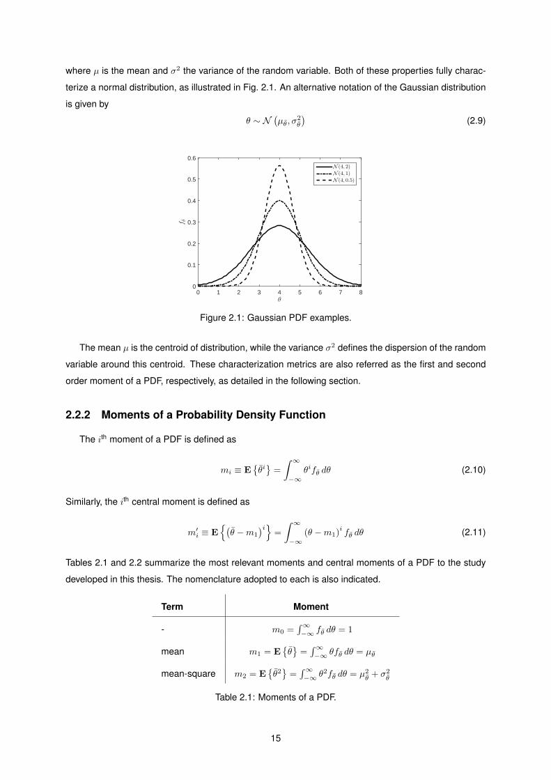
where µ is the mean and σ2 the variance of the random variable. Both of these properties fully charac-

terize a normal distribution, as illustrated in Fig. 2.1. An alternative notation of the Gaussian distribution

is given by

θ ∼ N(µθ, σ

2θ

)(2.9)

θ

0 1 2 3 4 5 6 7 8

fθ

0

0.1

0.2

0.3

0.4

0.5

0.6N (4, 2)

N (4, 1)

N (4, 0.5)

Figure 2.1: Gaussian PDF examples.

The mean µ is the centroid of distribution, while the variance σ2 defines the dispersion of the random

variable around this centroid. These characterization metrics are also referred as the first and second

order moment of a PDF, respectively, as detailed in the following section.

2.2.2 Moments of a Probability Density Function

The ith moment of a PDF is defined as

mi ≡ E{θi}

=

∫ ∞−∞

θifθ dθ (2.10)

Similarly, the ith central moment is defined as

m′i ≡ E{(θ −m1

)i}=

∫ ∞−∞

(θ −m1)ifθ dθ (2.11)

Tables 2.1 and 2.2 summarize the most relevant moments and central moments of a PDF to the study

developed in this thesis. The nomenclature adopted to each is also indicated.

Term Moment

- m0 =∫∞−∞ fθ dθ = 1

mean m1 = E{θ}

=∫∞−∞ θfθ dθ = µθ

mean-square m2 = E{θ2}

=∫∞−∞ θ2fθ dθ = µ2

θ+ σ2

θ

Table 2.1: Moments of a PDF.

15

Term Moment

- m′0 =∫∞−∞ fθ dθ = 1

- m′1 = E{θ − µθ

}=∫∞−∞

(θ − µθ

)fθ dθ = 0

variance m′2 = E{(θ − µθ

)2}=∫∞−∞

(θ − µθ

)2fθ dθ = σ2

θ

Table 2.2: Central moments of a PDF.

2.3 Estimation Theory

2.3.1 Kalman Filter

Start by considering a LTI system described by the following model

x(k+1) = Ax(k) +Bu(k) +Gw(k) (2.12a)

z(k) = Cx(k) + v(k) (2.12b)

where x(k) ∈ Rn denotes the system state, u(k) ∈ Rm its control input, z(k) ∈ Rq the measured output,

w(k) ∈ Rn the process noise input, and v(k) ∈ Rq the measurement noise. The noise vectors which are

white noise Gaussian sequences obey the following relations

E {w(k)} = 0 E{w(k)w(t)

T}

= Qδkt

E {v(k)} = 0 E{v(k)v(t)

T}

= Rδkt

(2.13)

A, B, and C are the state, input and output matrices, respectively, of appropriate dimensions. The

Kalman Filter, firstly introduced by Kalman [59], is an optimal linear filter in the sense that it minimizes the

mean-square state estimation error. Since it is also assumed to be an unbiased filter, i.e. E {x} = E {x},

part of the literature also refers to it as the minimum variance unbiased estimator, which is equivalent to

the previous definition under the unbiased condition. Formerly the optimization criteria is given by

x(k|k) = arg minx

Σ(k|k) = arg minx

Tr(E{

(x(k)− x(k|k)) (x(k)− x(k|k))T})

(2.14)

where x corresponds to the optimal estimate of x. To avoid misunderstandings, we clarify that x(k|i)

stands for the estimation of x at time k based on measurements up to time i, k ≥ i. In what follows we

provide the key equations that define the Kalman filter dynamics.

Prediction Step

x(k+1|k) = Ax(k|k) +Bu(k) (2.15)

Σ(k+1|k) = AΣ(k|k)AT +GQGT (2.16)

16

Filtering Step

x(k|k) = x(k|k−1) + L(k) [z(k)− Cx(k+1|k)] (2.17)

L(k) = Σ(k|k−1)CT[CΣ(k|k−1)CT +R

]−1(2.18)

Σ(k|k) = [I − L(k)C] Σ(k|k−1) (2.19)

Initial Conditions

x(0|−1) = x0 (2.20)

Σ(0|−1) = Σ0 (2.21)

The steady-state version of the Kalman filter may be derived under the following additional conditions

1. The matrix Q = QT is a positive definite matrix.

2. The matrix R = RT is a positive definite matrix.

3. The pair (A,G) is controllable (excitation condition).

4. The pair (A,C) is observable.

which enable the following conclusions

1. The prediction covariance matrix Σ(k|k−1) converges to a constant matrix,

limk→∞

Σ(k|k−1) = Σ

where Σ is a symmetric positive definite matrix, Σ = ΣT � 0.

2. Σ is the unique positive definite solution of the discrete algebraic Riccati equation

Σ = AΣAT −AΣCT[CΣCT +R

]−1CΣAT (2.22)

3. Σ is independent of Σ0 provided that Σ0 � 0.

A consequence of these conclusions is that the Kalman filter gain will tend towards a constant value

given by

L = limk→∞

L(k) = ΣCT[CΣCT +R

]−1(2.23)

and the filter dynamics will be time-invariant. For a more detailed deduction of this important result see

[54].

2.3.2 H2 Filter

TheH2 filtering problem, in its classical form, is defined as the deduction of a linear filter that ensures

estimation stability and minimization of the H2 norm of the transfer function from the noise inputs to the

17

estimation error. Based on the definitions presented in Section 2.1,it is then equivalent to minimizing the

mean-square estimation error, or more precisely the root-mean-square. Therefore, assuming x as the

estimation of the state vector x, the problem is formerly given by

x(k|k) = arg minx

Tr(E{

(x(k)− x(k|k)) (x(k)− x(k|k))T})

(2.24)

meaning that we recover the optimization criteria (2.14) defined for the Kalman filter design. As a

consequence, both filters are equivalent in performance and structure since the optimal filter solution

is unique, as expressed in the previous section. The great advantage of the H2 formulation is that it

allows to design an "optimal" filter for an uncertain system, i.e. systems that admit uncertainties in their

state-space matrices. In that case, the optimization criteria can be redefined to the minimization of the

upper bound of the mean-square estimation error over all the uncertainty domain. In simpler words,

it means that despite the parameters that the real model admits, it is ensured that the filter obtained

minimizes the mean-square error of the worst case scenario. Hence, defining by M the uncertain

model of the system, which we know to belong to the convex bounded polyhedral domain Dc, the formal

optimization criteria is defined by

x(k|k) = arg minx

[supM∈Dc

Tr(E{

(x(k)− x(k|k)) (x(k)− x(k|k))T})]

(2.25)

Usually this problem is solved through LMI semi-definite programming. We also stress that the latter

approach, concerning model uncertainty, is just one possible formulation. Other types of constraints

may also be defined including pole placement of the filter dynamics, as nicely highlighted by Rodrigues

[60]. Still, in this thesis only model uncertainty is considered due to the effect of faults on the system

parameters.

2.4 Linear Matrix Inequalities

Let Sn be the space of symmetric matrices with dimensions n × n. A Linear Matrix Inequality (LMI)

assumes de form

F (x) , F0 +

m∑i=1

xiFi � 0 (2.26)

where x ∈ Rm is the variable and Fi ∈ Sn are m given matrices. In words, a LMI may be defined as a

linear combination of symmetric matrices in the form of a inequality. These inequalities may either be

strict (� ,≺) or nonstrict (� ,�). Due to the linearity, LMIs are convex constraints on x, i.e. {x | F (x) � 0}

is convex. As a consequence, they are easily tractable and several tools are available to efficiently solve

problems built upon LMIs. This is specially interesting in control theory, namely in Lyapunov stability

theory in which the Lyapunov inequality is formulated as

ATP + PA ≺ 0 (2.27)

18

where A ∈ Rn×n is given and P ∈ Sn is the matrix variable. Note that the form here is not as explicit

as in LMI (2.26) definition, but that can be achieved by taking P1, . . . , Pm as the basis of the symmetric

n × n matrices followed by defining F0 = 0 and Fi = −ATPi − PiA. In this thesis, the use of LMIs will

be mostly focused on semi-definite programming in which a linear objective function is defined with LMI

constraints. The referred type of problem is intensively explored in Chapter 5 for the design of H2 filters.

To conclude, two important results related to LMI problem manipulation are given below. Both of which

will be relevant in the research developed.

Lemma 2.1. (Schur Complement) Consider X ∈ Sn a partitioned matrix as

X ≡

X1 X2

• X3

(2.28)

Then,X � 0 iff X1 � 0 and X3 − X2TX1

−1X2 � 0. Furthermore if X1 � 0 then X � 0 iff X3 −

X2TX1

−1X2 � 0.

Lemma 2.2. (Congruence Transformation) Two matrices X, Y ∈ Sn are said to be congruent if there

exists a nonsingular matrix T ∈ Rn×n such that Y = TTXTT . Furthermore if X and Y are congruent

then Y � 0 iff X � 0.

We will not enter in further details on this section concerning LMIs, but for the interested reader we

suggest two very well written books devoted to the topic of LMI problems applied to control [56, 57]. For

a less extensive reading, but very clarifying introductory approach see [58].

19

20

Chapter 3

Fault Model

Consider an LTI system of the form

x(t) = Ax(t) +Bu(t) (3.1a)

y(t) = Cx(t) +Du(t) (3.1b)

where x is the state, u the input, and y the output vectors of the system. Matrices A, B, C, and D

correspond, respectively, to the state matrix, input matrix, output matrix and feedthrough matrix. Usually

faults are modelled with a variation of the system parameters which directly affect the system matrices. In

fact, for several types of fault, the system defined by {A,B,C,D} can be replaced with {Af , Bf , Cf , Df}

in a fault condition by the following relations

Af = A+ δA; Bf = B + δB; Cf = C + δC; Df = D + δD; (3.2)

Still, as discussed in Chapter 1 this multiplicative modelling fashion is more suitable for component faults,

becoming restrictive if one intends to consider sensor or actuator faults. For instance, an offset fault that

imposes a bias in the state dynamics can not be described by formulation (3.2).

Figure 3.1: Types of actuator faults occurring after tF . Source: [30, pg. 6]

21

In this thesis the focus will be the study on actuator faults, which will require us to find an appropriate

additive fault model. Despite this particularization, it is aimed that the developed research can also

be applied to other types of faults by considering a dedicated fault model. In what follows, let us first

reason that an actuator fault can be seen as a modification of the system input vector u. Through the

reviewed literature, but mainly based on Jacques and Ducard [30], four major types of actuator faults

can be identified. All of which are illustrated in Fig. 3.1. Except for fault type (a), the other three types of

fault may be modelled by the combination of two scalar fault parameters: (i) an effectiveness parameter

λ ∈ [0, 1] and (ii) an offset parameter u0 ∈ [umin, umax] such that the system input may be given by

u(t) = Λuc(t) + u0 (3.3)

with

Λ = diag ([λ1, λ2, . . . , λm]) ; u0 = [u01, u02, . . . , u0m]T (3.4)

where m is the number of system actuators and uc the control input vector. The global actuator fault

system model is then given by

x(t) = Ax(t) +B (Λuc(t) + u0) (3.5a)

y(t) = Cx(t) +Du(t) (3.5b)

A fault domain representation is shown in Fig. 3.2 where each fault type region is indicated. Note

that in nominal/fault-free condition the following fault parameters matrices hold

Λ = diag(1m

T)

; u0 = 0m (3.6)

u0

λ

umin

umax

10

Locked-in-place

Hard-over

Hard-over

Loss of Effectiveness

Nominal/Fault-free

Figure 3.2: Actuator fault types illustrated in fault parameters domain.

22

Chapter 4

Multiple-Model Adaptive Estimation

(MMAE)

4.1 Properties of the MMAE

4.1.1 General Structure

The Multiple-Model Adaptive Estimation (MMAE) technique is a model-based estimation approach

specially suitable for systems subject to parameter uncertainty. If some information is known about the

uncertain parameter, such as its domain of uncertainty, then a multiple-estimator bank structure may

be designed covering an adequate range of possible models. A specific probability analysis tool may

then be applied to analyse the local state-estimation and associated innovations, for a stochastic setting,

generated by each estimator in order to obtain the optimal combined estimation. The architecture of the

described technique is shown in Fig. 4.1.

Plant

KF1

...

KFN

PosteriorProbabilityEvaluator

...

x1(k|k)

ν1(k|k)

xN (k|k)

νN(k|k)

u z

x(k|k)

P (k)

S1

SN

· · ·

MMAE

Figure 4.1: Multiple-model Adpative Estimation (MMAE) Architecture.

Recall that under no parameter uncertainty, the Kalman filter (KF) is the optimal state-estimation fil-

ter as shown by Rudolf E. Kalman [59] and several other authors [61, 62, 54] throughout the years. We

23

also know that under those ideal conditions and some linear-gaussian assumptions, explored in Sec-

tion 2.3.1, the KF provides the true conditional mean and covariance of the state vector given the past

control inputs and observations. Therefore, based on our assumptions about the uncertain parameters

set we may well design each estimator of the bank as a KF tuned for a certain admissible parameter

vector. Besides the bank of KFs, the MMAE has in its structure a Posterior Probability Evaluator which

owns the responsibility of determining how well each filter is performing at every time-step. This perfor-

mance information is provided as the conditional probability of each estimator model to match the real

system given the past sequence of measurements and inputs. The global state-estimate provided by

the MMAE is then the posterior probabilities weighted sum of each local estimate [63].

Note that we may interpret system faults as uncertainties in our model description, thus the MMAE

turns out to be an interesting tool under the scope of our study in fault detection and isolation. Ac-

cordingly, consider an LTI MIMO system subject to actuator uncertainties according to the actuator fault

model described in Chapter 3

x(k+1) = Ax(k) +B(Λκu(k) + uκ0

)+Gw(k) (4.1a)

z(k) = Cx(k) + v(k) (4.1b)

where x(k) ∈ Rn denotes the system state, u(k) ∈ Rm its control input, z(k) ∈ Rq the measured output,

w(k) ∈ Rn the process noise input, and v(k) ∈ Rq the measurement noise. The noise vectors, which are

white noise Gaussian sequences, obey the following relations

E {w(k)} = 0 E{w(k)w(t)

T}

= Qδkt

E {v(k)} = 0 E{v(k)v(t)

T}

= Rδkt

(4.2)

A, B, and C are the state, input and output matrix of appropriate dimensions, respectively. Matrix Λκ

and vector u0(k) are unknown and determine the uncertain parameters of system (4.1) that belong or

are "close" to a finite discrete parameter set, κ := {κ1, κ2, . . . , κn} indexed by i ∈ {1, 2, . . . , N}. The

MMAE approach suggests that the global estimate is given by

x(k|k) =

N∑i=1

Pi(k)xi(k|k) (4.3)

whereas the global residual covariance matrix is obtained by

Σ(k|k) =

N∑i=1

Pi(k)

[Σi(k|k) + (x(k)− xi(k|k)) (x(k)− xi(k|k))

T]

(4.4)

where Pi(k) stands for the conditional posterior probability of κi = κ, i.e. that estimator i model matches

the real system. It can be shown that if κ ∈ κ both Eqs. (4.3) and (4.4) represent the true conditional

expectation and conditional covariance of the state estimate; for details on that result see [64].

24

4.1.2 Posterior Probability Evaluator (PPE)

The central element of the MMAE is the previously referred Posterior Probability Evaluator (PPE)

which is responsible for computing the posterior conditional probability of each model, at every instant,

to match the real one. Considering the notation used in Section 4.1.1, this probability is equivalent to the

probability of κi = κ with i ∈ {1, 2, . . . , N} given by Pi(k). Due to the importance of the PPE module, the

recursive relation to compute those probabilities is now deduced, so that it can be implemented online.

Start by considering the formal description of the conditional probability which we aim to obtain

Pi(k) = P [κ = κi | Z(t)] ≥ 0 ,

N∑i=1

Pi(k) = 1 (4.5)

where κi ∈ {κ1, κ2, . . . , κN} := κ represents a certain model considered out of a set of N possible

models and Z(t) = [u(0),u(1), . . . ,u(k−1); z(1), z(2), . . . , z(k)] represents the available information until

instant k consisting of all the control input vectors u and measured output vectors z. One relevant

property is related to the probability density functions associated to Pi(k), which are a weighted sum of

impulses due to κ being a discrete random variable

p [κ|Z(k)] =

N∑i=1

Pi(k)δ (κ− κi) (4.6a)

p [κ|Z(k+1)] =

N∑i=1

Pi(k+1)δ (κ− κi) (4.6b)

Note that we may face our deduction by trying to develop a recursive algorithm which enables to obtain

Pi(k+1) from Pi(k). This way, consider the following deduction by applying Bayes’ rule

p [κ|Z(k+1)] = p [κ|u(k), z(k+1), Z(k)]

=p [κ, z(k+1)|u(k), Z(k)]

p [z(k+1)|u(k), Z(k)]

=p [z(k+1)|u(k), κ, Z(k)] · p [κ|Z(k)]

p [z(k+1)|u(k), Z(k)]

(4.7)

Replacing now Eq. (4.6a) in Eq. (4.7) and defining κ = κi we obtain the desired relation

Pi(k+1) =p [z(k+1)|u(k), κi, Z(k)]

p [z(k+1)|u(k), Z(k)]· Pi(k) (4.8)

The numerator in Eq. (4.8) corresponds to the probability density function of obtaining measurement

z(k+1) given a certain input u at time k and information Z until that instant while having model κi

matching the real plant. Recalling the definition of the ith Kalman Filter innovation vector νi(k+1) ∈ Rq

and the associated covariance matrix Si(k+1) ∈ Rq×q which are given by

νi(k+1) = z(k+1)− Cxi(k+1|k) ; E {νi(k+1)|u(k), κi, Z(k)} = 0 (4.9)

Si(k+1) = cov{νi(k+1)νi(k+1)

T |u(k), κi, Z(k)}

= CΣ(k+1|k)CT +R (4.10)

25

It can be easily shown that the referred PDF is Gaussian with mean

E {z(k+1)|u(k), κi, Z(k)} = Cxi(k+1|k) (4.11)

and covariance

cov{z(k+1)z(k+1)

T |u(k), κi, Z(k)}

= cov{νi(k+1)νi(k+1)

T |u(k), κi, Z(k)}

= Si(k+1) (4.12)

Therefore, the following relation may be obtained

p [z(k+1)|u(k), κi, Z(k)] =e−

12νi(k+1)TSi(k+1)−1νi(k+1)

(2π)m2

√detSi(k+1)

(4.13)

To complete our deduction, we still need to find an explicit relation for the denominator in Eq. (4.8)

p [z(k+1)|u(k), Z(k)] =

∫p [z(k+1), κ|u(k), Z(k)] dκ

=

∫p [z(k+1)|u(k), κ, Z(k)] p [κ|Z(k)] dκ

=

∫p [z(k+1)|u(k), κ, Z(k)]

N∑j=1

Pi(k)δ (κ− κj) dκ

=

N∑j=1

p [z(k+1)|u(k), κj , Z(k)] · Pj(k)

(4.14)

where the term p [z(k+1)|u(k), κj , Z(k)] is equivalent to Eq. (4.13). Usually the conditional probability

Pi(k+1) is also referred as the posterior whereas Pi(t) the prior. In conclusion, the explicit relation for

Eq. (4.8) is then expressed by

Pi(k+1) =

(ζi(k+1)e−

12ωi(k+1)∑N

j=1 ζj(k+1)e−12ωj(k+1)Pj(k)

)· Pi(k) (4.15)

with ζi(k+1) ≡ 1

(2π)m2

√detSi(k+1)

and ωi(k+1) ≡ νi(k+1)TSi(k+1)

−1νi(k+1)

for a given initial prior Pi(0). A closer look at Eq. (4.15) reveals that, from an implementation point of

view, one may not allow that any model κi has its probability down to 0 as it will cause the posterior

to never recover, even if κi matches the real model. Thus, the following criterion was defined in our

research

Pi(k) ≥ ε with ε = 10−4 (4.16)

Remarks

• Note that the covariance Si(k+1) is a pre-computable quantity which assumes the steady-state

value Si = CΣCT + R; for further details on this result see [61, p. 270]. Consequently, the scalar

value ζi(k+1) in Eq. (4.15) is also computed offline, as opposed to wi(k+1) which is a real-time

quantity.

26

• It is interesting to notice that similarly to the single-model approach, the past control sequence

[u(0),u(1), . . . ,u(k−1)] has a direct impact on the conditional state-estimate generated by the KF.

• On the other hand, contrarily to the single-model case, in the MMAE technique the past control

sequence influences the accuracy of the estimation by affecting the conditional global estimation

error covariance matrix Σ(k|k), as expressed in the above relations. As a consequence, this implies

that certain control sequences may induce an improved estimation performance [64].

4.1.3 Convergence Properties

This section explores the asymptotic properties of the MMAE. Until this point, we have constantly

considered that the real model parameter κ is in the discretized parameter set κ. Thus, our first object

of analysis should be to find a proof that if κ = κi, where κi denotes the design point of filter i inside

the bank, then its conditional posterior probability Pi(k) must asymptotically converge to 1, whereas

Pj(k) → 0 with j 6= i. In what follows, it is fair to assume that for a persistently excited system we

might expect that the innovation sequence of the ith Kalman Filter will be less energetic than the other

innovation sequences represented by index j 6= i

νi(k) << νj(k) ∀j 6= i (4.17)

Recovering the result found in Eq. (4.15), let us try to compute the conditional posterior probability

difference between time steps for model i

Pi(k+1)− Pi(k) =

(ζi(k+1)e−

12ωi(k+1)∑N


− 1

)· Pi(k)

=

((1− Pi(k)) ζi(k+1)e−

12ωi(k+1) −

∑Nj 6=i ζj(k+1)e−

12ωj(k+1)Pj(k)∑N


)· Pi(k)

(4.18)

With assumption (4.17), we can also state the following as k →∞

e−12ωi(k+1) → 1 (4.19a)

e−12ωj(k+1) → 0 ∀j 6= i (4.19b)

Consequently,

Pi(k+1)− Pi(k) =Pi(k) (1− Pi(k)) ζi(k+1)∑Nj=1 ζj(k+1)e−

12ωj(k+1)Pj(k)

> 0 (4.20)

By contrast for j 6= i,

Pj(k+1)− Pj(k) =−Pj(k)Pi(k)ζi(k+1)∑N


< 0 (4.21)

Results (4.20) and (4.21) show us the intended MMAE convergence properties, assuming the "nice"

innovation sequence behaviour as stated in Eq. (4.17). Moreover, we put forward the assumption that

the real model parameter is, indeed, inside the parameter set κ. The following natural step is therefore to

27

analyze the convergence properties of the MMAE in case the uncertain parameter domain is infinite or

just too large to be fully covered by the model set. We stress that this analysis is crucial to our research

on fault detection, on the basis that the actuator fault model applied (Chapter 3) provides us an infinite

but bounded uncertain parameter set. In [61, p. 274] an interesting discussion is developed on this issue

from where we borrow the following theorem.

Theorem 4.1. [61, p. 274] With notation as above, let the true value of κ be κ0 and let νi(k) for

κ := {κ1, κ2, . . . , κn}, indexed by i ∈ {1, 2, . . . , N}, be the innovations sequence of the Kalman Filter

tuned to κi and driven by the real model input and output. Let Si(k) denote the design covariance of

the filter innovations, i.e., the value of E{νi(k)νi(k)

T}

should the real model have κ = κi. Suppose that

νi(k) is asymptotically ergodic in the autocorrelation function; suppose that Si(k) → Si as k → ∞ with

Si > 0; and denote the actual limiting mean-square innovations1 of the filter by

Γ0i ≡ lim

n→∞n−1

k+n−1∑j=k

νi(j)νi(j)T (4.22)

Suppose that a priori pseudo-probability P1(0), P2(0), . . . , PN (0) are assigned, with Eq. (4.15) providing

the recursive update for these pseudo-probabilities. Define

β0i = ln (detSi) + Tr

(Si−1Γ0

i

)(4.23)

and assume that for some i, say i = I ∀j 6= I, one has

βI < βj (4.24)

Then PI (k)→ 1 and Pj(k)→ 0, as k →∞ with convergence being exponentially fast.

Proof. [61, p. 274]

From Theorem 4.1 one may conclude that for the case that none of the models included in the bank

of filters matches the real parameters, the MMAE will converge to the closest matching model in a proba-

bilistic sense, defined by Eq. (4.23). This equation is also commonly referred to as the Baram Proximity

Measure (BPM) [65, 66, 43] and plays an important role within the MMAE bank design discussed in

Section 4.3. In other words, one may say that if the uncertain parameter κi is the representation of the

true model, then the MMAE governed by Eq. (4.15) will converge to the jth filter whose BPM satisfies

βij = minj

βij ∀j ∈ {1, 2, . . . , N} (4.25)

Moreover, the actual mean-square innovations generated by each filter are given by Eq. (4.22) determin-

ing the accuracy of the estimation generated. Also, it is stressed that in this scenario Eqs. (4.3) and (4.4)

provide no longer the true conditional expectation and conditional covariance of the state estimate, but

still the most truthful expectation owing the convergence result discussed in this section.1In [61] the author uses the term covariance. In order to keep the mathematical formalism, it was decided to not apply it here

since in general the innovation sequence is not white so long as κ 6= κi.

28

4.1.4 Computing the mean-square innovation generated by each filter

A demonstration for the computation of the actual limiting mean-square innovation Γ is now provided.

That being said, consider both the true model representation for which we admit a determined parameter,

say κi

x(k+1) = Ax(k) +B(Λiu(k) + ui

0

)+Gw(k) (4.26a)

z(k) = Cx(k) + v(k) (4.26b)

and a Kalman Filter model tuned for a generic parameter κj

xj(k+1|k) = Axj(k|k) +B(

Λju(k) + uj0

)(4.27a)

xj(k+1|k+1) = xj(k+1|k) + L (z(k+1)− Cxj(k+1|k)) (4.27b)

where the notation used previously in description (4.1) is preserved and L ∈ Rn×q stands for the Kalman

Filter gain. Let the mean-square innovation generated by Kalman Filter (4.27) fed by the input and output

of system (4.26) be given by

Γij(k) ≡ E{ν(k)ν(k)

T}

= E{

(z(k)− Cx(k|k−1)) (z(k)− Cx(k|k−1))T}

(4.28)

being our variable of analysis. We stress that for the scenario κi = κj , the steady-state mean-square

innovation generated by the filter, i.e. the steady-state solution of Eq. (4.28), is equivalent to the optimal

innovation covariance given in Eq. (4.10). Consider now the combined dynamics of the system state

x(k) and its predicted estimation xj(k|k−1) by

x(k+1)

xj(k+1|k)

=

A 0

ALC A(I − LC)

x(k)

xj(k|k−1)

+

BΛi

BΛj

u(k) +

Bui0

Buj0

+

G 0

0 AL

w(k)

v(k)

(4.29)

Hereafter, assume a generic stabilizing control law u(k) = −Kz(k) to be applied to the dynamics de-

scription x(k+1)

xj(k+1|k)

=

A−BΛiKC 0

ALC −BΛjKC A(I − LC)

x(k)

xj(k|k−1)

+

Bui0

Buj0

+

G −BΛiK

0 AL−BΛjK

w(k)

v(k)

(4.30)

29

where for notation convenience

xj(k) ≡

x(k)

xj(k|k−1)

(4.31)

F ij ≡

A−BΛiKC 0

ALC −BΛjKC A(I − LC)

(4.32)

uij ≡

Bui0

Buj0

(4.33)

Gij ≡

G −BΛiK

0 AL−BΛjK

(4.34)

n(k) ≡

w(k)

v(k)

(4.35)

Hence, Eq. (4.30) is notationally simplified to

xj(k+1) = F ijxj(k) + uij +Gijn(k) (4.36)

Eq. (4.28) can also be written in the following alternative form

Λij(k) =[C −C

]E

x(k)

xj(k|k−1)

x(k)

xj(k|k−1)

T[C −C

]T+R = HΨi

j(k)HT +R (4.37)

Assuming an asymptotically stable dynamics matrix F ij , the steady state limit of Ψij(k) → Ψi

j as k → ∞

can be computed and is generated by the discrete-time Lyapunov function

Ψij = F ijΨ

ijF

ij

T+ T +GijNG

ij

T(4.38)

with

N ≡ E{n(k)n(k)

T}

=

Q 0

0 R

(4.39)

and

T ≡ F ijE {xj(k)}uijT

+ uijE{xj(k)

T}F ij

T+ ui

juij

T(4.40)

= F ij(I − F ij

)−1uiju

ij

T+(F ij(I − F ij

)−1uiju

ij

T)T

+ uiju

ij

T

Finally the sought relation for the steady-state mean-square innovation is then given by

Γij = HΨijH

T +R (4.41)

30

4.2 Advantages and Limitations of the MMAE

In the last decades, the MMAE methodology has been studied and applied by several authors in the

realm of fault detection, fault isolation and reconfigurable control systems [67, 28, 27, 30, 9]. The interest

in this technique find its primary reason on the capacity of coping with any type of parameter variation

the designer may consider and fast responsiveness to faults due to the multiple-model structure [27].

Also, the capability of not only detecting and isolating faults but, also enabling the reconstruction of a

correct state estimate is of high importance to the application of commonly used control algorithms.

On the other hand, this multiple-model approach also presents a set of drawbacks worth to be dis-

cussed. The MMAE design follows the idea that each KF is tuned to a specific fault. Therefore, usually

they are not representative of the whole range of possible faults but only of the most probable ones

based on some knowledge about the system. For instance, in the borrowed helicopter presented in

Appendix A, which includes four actuators, we would require one KF for every possible fault position per

actuator just for the lock-in-place type of fault. It would be impracticable to consider one estimator for ev-

ery combination of fault magnitude and fault type per actuator. Not to mention other sources of incidents

such as sensor faults or component faults. Considering this remark, in certain unexpected scenarios the

estimation provided by the filters can be completely biased and become useless for control purposes.

Frequently, even if just considering the most probable fault scenarios, some implementation issues may

be found such as the demanding computation load to process a large bank of Kalman filters. Although

search and development of rather efficient and faster processors have been a focus of study on the last

decades, allowing this method to regain prominence in recent times [30], there will always be a limit to

the size of the bank of estimators.

As a final consideration, it should be mentioned that the MMAE methodology assumes that the

change of model is infrequent. This means that the convergence of hypotheses must be faster than

the modification of the real model, otherwise no guarantees are provided concerning the reliability of

the method [64]. Still, under the FDI framework this might not represent a main concern by noting that

system faults are usually improbable and barely occur sequentially in small time intervals.

4.3 Bank of Kalman Filters Design Strategy

As stated earlier, the actuator fault model which we consider provide us with an infinite uncertain

parameters set. From this set one shall pick N admissible values which will be the tuning parameters of

our N Kalman filters. In what follows, two main questions arise in this design process

1. What should be the size of the representative parameter set given by N which define the number

of KFs in the bank?

2. How can one establish the representative parameter set κ := {κ1, κ2, . . . , κN} ?

Before facing the design problem to answer these two questions, let us first introduce the important

concept of EIP and discuss a few details about the estimators’ bank properties and about a relevant

31

design procedure assumption.

4.3.1 Defining the concept of Equivalently Identified Plants (EIP)

Since we are dealing with an infinite uncertain parameters set, we can not assume that the real fault

parameter, represented by κ, will be inside κ. However, from the convergence results presented in Sec-

tion 4.1.3 one knows that the closest matching model in a probabilistic sense defined by the Baram Prox-

imity Measure (BPM) metric will have its probability, say Pi, converging to 1 while the others, Pj ∀j 6= i,

will converge to 0. This property allows us to define regions in the uncertain parameter domain that are

characterized by the model to which they will converge given all the admissible real parameter and the

representative set κ. Each of these regions is called the set of Equivalently Identified Plants (EIP) [45].

An exemplification of this representation is given in Fig. 4.2 considering a bi-dimensional limited param-

eter uncertainty, which is equivalent to our design problem as will be discussed later in this section. It is

noticed that each EIP region is represented by a well-defined boundary and the parameter to which the

associated KF model is tuned - κ1, κ2, κ3, κ4.

θ2

θ1

θ−2

θ+2

θ−1 θ+1

κ1 =⟨θ11 , θ

12

⟩

θ11

θ12

EIP1

κ2

EIP2

κ3

EIP3

κ4

EIP4

Figure 4.2: Equivalently Identified Plants (EIP) representation example for a bi-dimensional uncertaintyparameter κ =

⟨θ1 ∈

[θ−1 , θ

+1

], θ2 ∈

[θ−2 , θ

+2

]⟩.

4.3.2 Equivalent Kalman Filter Dynamics

Given our system model in (4.1) we may note that the uncertain parameters only affect the control

input elements, meaning that the Kalman Filter dynamics are equivalent for every tuning parameters

in the model set. Recall that the Kalman Filter minimizes the estimation error covariance considering

the stochastic inputs, given by w(k) and v(k). Since the system dynamics matrix A is not affected as

well as matrix G, then the transfer function from the noise inputs to the estimation error is not modified

for any admissible uncertain parameters. This is not true in general for other types of faults, such as

component faults which may affect, for instance, the dynamics matrix. Moreover, given that our system

is time-invariant from the filters perspective and under a few additional assumptions [54], in steady-state

the Kalman gain is constant and the filter dynamics is also time-invariant. Similarly, the steady-state

32

estimation error and innovation covariance matrices are again constant. As a consequence of this anal-

ysis, the optimal performance of every EIPi is equivalent, occurring when κ = κi, and is given by the

innovation covariance Si ≡ S ∀κi ∈ κ; see remark 1 on Section 4.1.2.

4.3.3 Independent Bank Design per actuator

We finally stress that our design procedure considers each actuator individually, i.e. for every model

the uncertain domain is characterized by only two scalar uncertain parameters λj and u0j with j ∈

{1, 2, . . . ,m} indexing the actuator under analysis. The reason for this strategy lies in the convenience

of performing the bank design in a R2 domain, rather than a larger dimension domain. Therefore, the

idea is to run a design methodology for each actuator and create a bank of KFs generated by the union of

the sub-banks designed for each actuator fault model. This way, the design of the sub-bank considering

the model uncertainty on actuator j assumes

Λj = diag ([λ1, λ2, . . . , λm]) (4.42)

with λn =

1 for n 6= j

λj ∈ [0, 1] for n = j

∀n ∈ {1, 2, . . . ,m}

uj 0 = [u01, u02, . . . , u0m]T (4.43)

with u0n =

0 for n 6= j

u0j ∈ [−1, 1] for n = j

∀n ∈ {1, 2, . . . ,m}

Being the uncertain parameters vector given by

κ = 〈λj , u0j〉 (4.44)

As a result, system (4.1) for the ith Kalman Filter with an admissible fault in actuator j may be rewritten

as

x(k+1) = Ax(k) +B(

Λj iu(k) + uj i0

)+Gw(k) (4.45a)

z(k) = Cx(k) + v(k) (4.45b)

4.3.4 Design Procedure

Having discussed the relevant preliminary aspects in the prequel, we shall now focus on the design

procedure. The first step towards this design, is to reason that the ideal way to deal with the questions

stated in the beginning of the section would be to have a performance measure that could allow us

to define the discretized representative parameter set κ in a systematic procedure. In [45], the author

33

suggests a performance-based model set design strategy for the MMAE, in a one dimension parameter

vector framework. The presented strategy introduces the concept Infinite Model Adaptive Estimation

Performance (IMAEP) index which provides the best performance in terms of Baram Proximity Measure

considering an ideal bank design with N → ∞. The IMAEP may be obtained by computing Si in

Eq. (4.23)

βii ≡ βi = ln (detSi) +q

2(4.46)

where q stands for the dimension of the measurement vector z(k), as identified in (4.1). Indeed, this

corresponds to the scenario of having the true parameter vector κ = κi, being κi part of the represen-

tative parameter set κ. The designer input to this approach is provided as a percentage of Eq. (4.46),

% IMAEP, which defines the worst admissible performance. Consequently, every covered parameters in

a EIP region, say EIPj , must satisfy

βi ≤ βij ≤ %βi (4.47)

being κi the considered real parameter vector and κj the closest parameter vector in the bank, in terms

of BPM. As an example see Fig. 4.3, which considers a one dimension parameter vector known to

be inside a domain region limited by κ− and κ+. The algorithm starts in one of the domain limits,

and progressively computes the BPM values until it reaches the opposite limit with a minimum number

models which satisfy the performance interval imposed by the % IMAEP curve. In our problem this

curve admits a constant value since Si = S is equal for every admissible κi as discussed previously,

nonetheless in general that is not the case. As a consequence of the design strategy introduced, we

are able to easily answer both questions presented in the beginning: how each parameter included in

the model set is chosen and consequently, the set size. Moreover, this performance-based design also

provides an intuitive manner of interpreting the design process.

βκκi(BPM)

κκ− κ+

EIP1 EIP2 EIP3

κ1

Model 1κ2

Model 2κ3

Model 3

IMAEP ≡ βκκ

% IMAEP ≡ %βκκ

βκκ1βκκ3

βκκ2

Figure 4.3: Representative parameter set definition via IMAEP approach for a one-dimension uncertaintyparameter domain.

Recall that in a bi-dimensional uncertain parameter domain, which characterizes our actuator fault

model, the BPM curves will become surfaces. Although the baseline idea is preserved, this fact forces

34

us to adapt the performance-based algorithm exploited. The first aspect to notice is that the intersection

between two surfaces is a curve and no longer a point as depicted in Fig. 4.3. A second challenge

imposed is that it is no longer straightforward how to define a progression direction between each de-

fined model. For the simplified one-dimension counterpart, once one started at one of the limits of the

uncertain parameter domain the only and obvious progression direction would be to the opposite limit.

Therefore, a few additions and small modifications were implemented. Firstly, it was settled that under

the scope of our study it is immediate that one of the models to be included is the nominal model, defined

by κ0 = 〈1, 0〉 based on the formulation provided in Eq. (4.44). Hence, this was defined as the initial point

from our model set "search" problem. At a second stage it was also reasoned that a fair progression

direction could be the straight line connecting the nominal parameter vector point κ0 and one of the most

extreme2 fault models to be admitted, κ+e = 〈0, 1〉 or κ−e = 〈0,−1〉3. The defined strategy is illustrated

in Fig. 4.4. Obviously this design procedure admits an infinity of variations considering the 180 degree

window from the nominal point, hence no guarantees are given in terms of minimization of the model set

size for a given performance criterion. It should be mentioned that no similar bi-dimensional uncertainty

MMAE bank design problem was found in the investigated literature, therefore we address it for future

research due to its relevance. An important remark shall be given concerning the approximated uncer-

tainty domain considered and revealed in Fig. 4.4 by the parameter λε. This approximation is related to

the necessity of ensuring the stability of F ij which is only possible for λ > 0. Note that λ = 0 cancels the

control law admitted in Eq. (4.30). In the results presented afterwards it was defined λε = 0.1.

u0

λ

−1

1

10

κ0

κ+e

κ−e

λε

Approx. Uncertainty DomainProgression Direction

κ0 Nominal Parameter Vectorκ±e Extreme Parameter Vector

Figure 4.4: Model-set design strategy illustration.

2The word extreme is used here in the sense that those points provide the largest norm difference to the nominal model in theuncertain parameter vector domain, i.e. ‖κe − κ0‖2 > ‖κ− κ0‖2 ∀κ 6= κe

3Recall that, in the borrowed helicopter model, umax = 1 and umin = −1.

35

Finally, we stress that the solution of the discrete-time Lyapunov function given in Eq. (4.38) shows

a symmetry of results on the effectiveness parameter λ axis, turning indifferent the choice between the

two alternative progression directions presented in Fig. 4.4.

4.3.5 Design Results

The results obtained from the estimators’ bank design are now presented. Due to the independence

of design of each actuator, we only considered in this process the first actuator - δB (cyclic control input)

- fault model in the helicopter system studied, which is deemed sufficient to validate the developed

technique. Two distinct performance criteria were chosen: 80% IMAEP and 50% IMAEP, whose results

are found in Figs. 4.5 and 4.6, respectively. As expected the former criterion revealed the need for a

larger amount of filters, 15 in total, whereas when defining 50% IMAEP as minimum performance 9 filters

were obtained. Each of the figures show two graphs. The first one (Fig. 4.5a;Fig. 4.6a) presents a 2D

view of the model set providing a clear view of the discretized representative set and each associated

EIP region with a gradient colouring to represent BPM levels. The second plot (Fig. 4.5b;Fig. 4.6b)

displays a 3D perspective of the surfaces with the performance measure, i.e. the BPM, on the third axis.

Finally, a table (Table 4.1;Table 4.2) is also given providing the exact location of each parameter vector

in the model set.

κ0 κ1/2 κ3/4 κ5/6 κ7/8 κ9/10 κ11/12 κ13/14

λ 1 0.69 0.48 0.34 0.24 0.18 0.13 0.1u0 0 ±0.31 ±0.52 ±0.67 ±0.76 ±0.82 ±0.87 ±0.90

Table 4.1: Model set obtained for a 80% IMAEP minimum performance criterion.

κ0 κ1/2 κ3/4 κ5/6 κ7/8

λ 1 0.53 0.28 0.15 0.10u0 0 ±0.47 ±0.72 ±0.85 ±0.90

Table 4.2: Model set obtained for a 50% IMAEP minimum performance criterion.

36

(a) 2D view

(b) 3D view

Figure 4.5: Bank of Kalman Filters design for a 80% IMAEP minimum performance criterion.

37

(a) 2D view

(b) 3D view

Figure 4.6: Bank of Kalman Filters design for a 50% IMAEP minimum performance criterion.

38

4.4 Experiments on Simulation Environment

This section aims to present the results of the simulations tests performed on the MMAE approach.

It is recalled that the following experiments were performed based on the helicopter system model pre-

sented in Appendix A. On this battery of simulations the estimators’ bank designed with a 50% IMAEP

criterion was applied and run for about 300 seconds along with the incidence of 4 distinct abrupt faults,

randomly chosen, at different instants. These faults are clearly characterised in Table 4.3 and associated

locations on the EIP regions are shown in Fig. 4.7. In the time between the faults incidence, which lasts

30 seconds for each, the nominal model is applied.

For this simulation setup, three main assessment goals were settled:

1. Evaluate the identifiability of the models by verifying the conditional posterior probability conver-

gence to different models along with the faults incidence and removal.

2. Compare the converged models with the expected results arisen from the estimators’ bank design;

see Fig. 4.7.

3. Verify that the performance criterion 50% IMAEP defined is satisfied.

These three assessment points not only enable us to validate the MMAE approach for actuator faults

detection purposes, but also allow to obtain an indicative validation of the bank of Kalman filters design

developed in Section 4.3.

Fault 1 (F#1) Fault 2 (F#2) Fault 3 (F#3) Fault 4 (F#4)λ 0.60 0.50 0.80 0.15u0 0.47 −0.90 0 0.7EIP 1 4 0 5Occurrence Time 30s-60s 90s-120s 150s-180s 210s-240s

Table 4.3: Faults description.

39

Figure 4.7: Faults on the EIP regions graph.

4.4.1 Results

1. Figure 4.9 displays the conditional posterior probability of each of the nine models included in the

bank of Kalman filters. A zoom-in view of the same information for the most relevant models owing

the faults properties is provided in Fig. 4.10. Analysing the initial moments, one may see that the

system clearly identifies the nominal model as the true model, until the first fault (F#1) occurrence

at instant 30s. As depicted in the correspondent zoom-in view, the convergence to the 1st Kalman

filter is achieved rapidly. However, some oscillations during the 30s of fault incidence are noticed.

Fault 2 (F#2) occurs at instant 90s and a probability convergence is also verified for model 4. In this

case, the oscillatory behaviour is even more evident due to a frequent probability exchange with

model 2. Note that the closest non-overlapping EIP region to fault 2 parameter vector is, indeed,

EIP2.

Fault 3 (F#3) is specially interesting because its parameter vector is located in the same EIP region

as the nominal model. Therefore, from instant 120s to 210, P0(k) is kept closer to 1, despite the

fault incidence at second 150.

Finally, fault 4 (F#4) causes an initial convergence to model 3, which is the closest non-overlapping

EIP region. Still, a few seconds later (≈ 5s) the identification of model 4 is attained matching the

expectations of the bank design.

2. In order to assess the MMAE system performance and compare it with the expected results, a

second experiment was run for each fault considering a unique incidence right at instant 1s. The

results obtained are presented in Fig. 4.8. It is clear that for every fault the performance metric

converges to a value between the IMAEP and 50% IMAEP. Moreover, the closer, in BPM terms,

the fault parameters are to the convergent filter parameters the better the performance achieved.

40

To analyse the latter aspect compare Fig. 4.8 and Fig. 4.7.

Figure 4.8: Real-time Baram Proximity Measure (BPM), performance criterion defined for the bankdesign and optimal performance IMAEP.

Comments on the Results

• The performed experiments show that the MMAE approach allows to clearly identify different mod-

els under distinct fault occurrences. Nevertheless, some faults, such as F#3, may not be detected

if their fault parameters fall in the nominal EIP region.

• An oscillatory behaviour of the conditional probabilities was verified at some instants, hence the

analysis of the these probabilities requires proper care. If some filter presents a high probability at

some moment, we may not assume directly that it corresponds or it is tuned to the closest model,

in a stochastic sense, to the real counterpart.

• The two previously analysed facts suggest that the MMAE approach is not an ideal tool for fault

detection and isolation, as it is susceptible to false alarms or missed detections. On the other

hand, it is a powerful system for state estimation under parameter uncertainty. Note that a good

state estimation is crucial for the performance of the control systems, which we aim to adapt on

the long run under a fault occurrence scenario.

• Fig. 4.8 provides an indicative validation for the performance-based design of the estimators’ bank.

This is, indeed, a convincing argument for the application of the MMAE method along with the

developed design strategy, since we are able ensure a well-defined a performance criterion for the

state estimation.

4.4.2 Improving results: second filtering stage

For some control algorithms that rely on the MMAE technique for state estimation, the posterior

probabilities are used to select which controller is put in practice at every instant; see [67] for details on

41

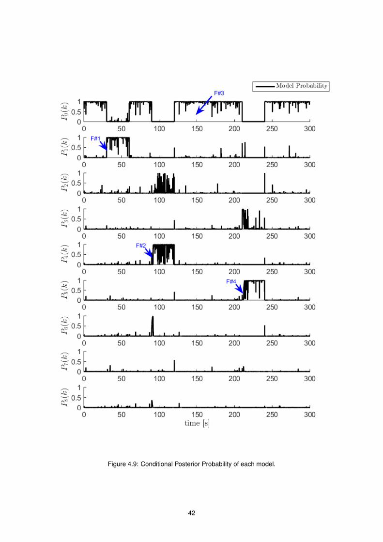
Figure 4.9: Conditional Posterior Probability of each model.

42

Figure 4.10: Zoom-in view: Conditional Posterior Probability of each model.

43

multiple-model adaptive control (MMAC) methods. Therefore, the observed oscillatory behaviour of the

conditional posterior probability signals is not completely suitable. Also, it does not meet what we initially

expected that was a clear identification of the models once a fault is defined in a certain EIP region.

KF1

...

KFN

Posterior

Probability

Evaluator

...Probability

Filtering

x1(k|k)

ν1(k|k)

xN (k|k)

νN(k|k)

u

z x(k|k)

P (k) P (k)

S1

SN

· · ·

MMAE

Figure 4.11: Inclusion of a second filtering stage in the MMAE architecture.

To enhance the obtained probability signals, a second filtering stage was developed based on an

original algorithm that only sets a certain model probability to 1 if it meets a defined criterion. The same

logic is applied to change the probability of some model back to 0. In practice, the algorithm outlined in

Fig. 4.12 gives a punctuation to every model in the bank based on its current probability. If it is higher

than an upper threshold, the model punctuation is increased by one, if it is less than a lower threshold

defined it sees its score decreased by one. All the models in-between both thresholds get 0 points. In

the end, the model with the highest score at every time-step is defined as the current identified model.

To avoid the domination of some model due to a longer period under the same working condition, maxi-

mum and minimum punctuation limits are imposed.

The outcome of the presented strategy, whose results are found in Figs. 4.13 and 4.14, is a well-

defined identification of the models. However, we highlight that the probability transition between filters

might take a longer time and that wrong isolations, i.e. probability transitions to not expected models,

might not be completely eradicated. In fact, in the performed simulation an erroneous isolation is ob-

served after fault 4 (F#4) incidence in which model 3 was expected to converge to 1. The same is

noticed for fault 2 (F#2). Still, a proper tuning of the algorithm variables, e.g. the thresholds and score

limits, might attenuate this drawback. We stress that the unfiltered probability signals are still used for

estimation purposes despite the filtering stage, as well expressed in Fig. 4.11, since they guarantee the

optimal estimation under our uncertainty regime.

To conclude, it is relevant to mention that similar filtering approaches have been undertaken in the

past by other researchers. Although not applied to probability signals, but to residual sequences, we

refer in this context the work developed by Ahmet [68].

44

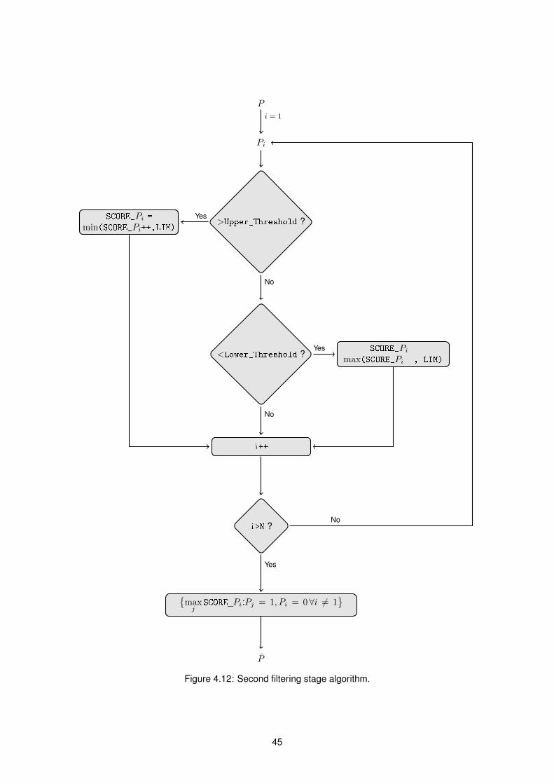
P

Pi

>Upper_Threshold ?SCORE_Pi =min(SCORE_Pi++,LIM)

<Lower_Threshold ?SCORE_Pi =

max(SCORE_Pi--,-LIM)

i++

i>N ?

{maxj

SCORE_Pi:Pj = 1, Pi = 0∀i 6= 1}

P

i = 1

Yes

Yes

No

No

Yes

No

Figure 4.12: Second filtering stage algorithm.

45

Figure 4.13: Filtered Conditional Posterior Probability of each model.

46

Figure 4.14: Zoom-in view: Filtered Conditional Posterior Probability of each model.

47

48

Chapter 5

Multiple-Model Adaptive Estimation

(MMAE) with H2 Robust Filters

5.1 Motivation for H2 Robust Filtering

In the last chapter we focused our study on fault diagnosis in a multiple-model based approach

which considered a bank of Kalman Filters, each specifically tuned for a fixed combination of actuator

fault effectiveness and offset parameters. The developed strategy, which was built upon a well defined

performance criterion, resulted in large banks of estimators capable of detecting and isolating faults ef-

fectively. To be more precise, the MMAE posterior probability evaluator could clearly indicate the real

fault parameters region when under a fault occurrence or in a fault-free scenario.

One of the drawbacks identified of the accomplished designed was the requirement for a large num-

ber of Kalman Filters to achieve the performance criterion defined. Recall that under the most strict

performance defined - 80% IMAEP - 15 filters needed to be included, whereas for the 50% IMAEP case

9 filters were required just for a single actuator monitoring. The use of a large number of estimators

asks for substantial processing means which are not always available and may well be limited in real

applications. This concern and the interesting studies about optimal linear filtering under parameter

uncertainty reviewed on the literature ([55, 69]) motivated the application of H2 robust filters under the

scope of actuator fault diagnosis.

The goal is set to reduce the number of filters required, while meeting a certain worst-case perfor-

mance. Note that the Kalman Filters designed in the previous chapter can be interpreted as H2 filters

in the sense that they also minimize the 2-norm of the estimation error output, or in other words the

steady-state estimation error covariance. The main difference between the two approaches is that with

the H2 synthesis the dynamical model of the system does not have to be precisely known, allowing to

cope with parameter uncertainties. Consequently, assuming that the estimation error depends on the

unknown parameters, the performance index to be optimized is the upper bound of the mean-square

49

estimation error, being valid for all admissible models [69]. In simpler words, the H2 synthesis guar-

antees "optimality" for a defined parameter uncertainty region instead of a single admissible operating

point. As a result, we may expect a reduction in performance in the Kalman Filter design points and

their neighbourhood but an equivalent or enhanced overall and worst-case performance with the bonus

of a bank size reduction. Fig. 5.1 illustrates the described expectation for a unidimensional parameter

uncertainty scenario, in which the performance of two Kalman Filters - tuned for z1 and z2 - is compared

with that of a single H2 filter optimized for the whole uncertainty region z ∈ [z−, z+].2-

Nor

mof

the

Est

imat

ion

Err

or

z

Performance Criterion

z− z+z1 z2

KF1 KF2

H2

Figure 5.1: Expectation about Kalman Filter-based vs H2-based MMAE design.

An alternative but also valid interest for the H2-based design could be to improve the overall perfor-

mance of each of the EIP regions defined in the previous chapter. With this strategy, despite considering

the same number of filters, an improved general performance might be attained revealing an optimiza-

tion of the performance criterion for an equivalent computational cost. Although that analysis falls out

of the scope of this thesis, for controller reconfiguration schemes it might be interesting sometimes to

preserve the EIP regions. For instance, Maybeck and Stevens [67] present a multiple-model adaptive

control (MMAC) algorithm which uses a separate set of controller gains specifically designed for every

admissible operating region determined by the MMAE EIP regions. It is straightforward that less regions

may impose a more changeling controller design, since it will have to be prepared to work under a larger

uncertainty scenario [67].

To conclude, we stress that the focus will be on reducing the number of required filters in the MMAE

bank, while simultaneously preserving or improving the performance criterion defined in Chapter 4.

50

5.2 H2 Robust Filter Design with LMI Convex Programming

5.2.1 General Case

Let us define the following discrete linear time-invariant system

x(k+1) = Ax(k) +Gn(k) (5.1a)

z(k) = Cx(k) +Dn(k) (5.1b)

ξ(k) = Cξx(k) (5.1c)

where x(k) ∈ Rn denotes the system state, z(k) ∈ Rq the measured output, n(k) ∈ Rn+q the noise

input, and ξ(k) ∈ Rs the vector to be estimated. The noise input is given by the concatenation of the

process noise input vector w(k) ∈ Rn and the measurement noise input vector v(k) ∈ Rq, which are

both uncorrelated white noise Gaussian sequences obeying the following relations

E {n(k)} =

E {w(k)}

E {v(k)}

=

0

0

E{n(k)n(k)

T}

=

E{w(k)w(k)

T}

0

0 E{v(k)v(k)

T} =

Q 0

0 R

≡W(5.2)

A, G, C, and Cξ are, respectively, the state, noise input, output, and estimation matrices of appropriate

dimensions. It is assumed that:

1. All matrices dimensions are known.

2. The parameter uncertainty of the system is characterized by a convex bounded polyhedral domain

Dc ⊃M, whereM∈ R(n+q)×(n+n) is defined as

M =

A G

C D

(5.3)

From [70], each uncertain matrix of this set can be written as an unknown combination of N given

extreme matricesM1,M2, . . . ,MN , resulting in the condition thatM∈ Dc if and only if

M =

N∑i=1

λiMi (5.4)

with λi ≥ 0 and∑Ni=1 λi = 1.

3. MatrixM is time-invariant.

4. Matrix Cξ is known and defined by the designer.

It should be emphasized that the description provided in assumption 2 is sufficiently general to allow

the modelling of any type of system uncertainties in the system matrices. In this thesis, uncertainties

51

are a surrogate for system faults, thus they can be easily considered by the provided description. This

is specially relevant for actuator effectiveness faults which directly affect the input matrix disguised in

matrix A through the control law. Accounting for offset faults in the actuators using this methodology is

addressed in the subsequent section.

Having defined the system and uncertainty domain, let us now consider the problem at hand. The goal

is to obtain an estimate ξ of ξ, through a linear filter F ∈ C which guarantees the minimum upper-bound

of the steady-state mean-square estimation error, e(k) = ξ(k) − ξ(k), over all the admissible parameter

uncertainty domain. Formally the objective function is given by

arg minF

[supM∈Dc

E{e(k)e(k)

T}]

(5.5)

which is also equivalent to the minimization of the H2 norm of the transfer function from the noise input

to the estimation error. Domain C represents the feasible set of all linear operators of order nf = n and

form

x(k+1) = Af x(k) +Bfz(k) (5.6a)

ξ(k) = Cf x(k) (5.6b)

where matrices Af ∈ Rnf×nf , Bf ∈ Rnf×q, and Cf ∈ Rs×nf are to be determined. Considering the

combined dynamics of system (5.1) and filter (5.6), we can write

x(k) = Fx(k) + Gn(k) (5.7a)

e(k) = Hx(k) (5.7b)

with

x(k) ≡

x(k)

x(k)

(5.8)

F ≡

A 0

BfC Af

(5.9)

G ≡

G

BfD

(5.10)

n(k) ≡

w(k)

v(k)

(5.11)

H ≡[Cξ −Cf

](5.12)

In what follows, it can be easily shown that the steady-state mean-square estimation error satisfies

limk→∞

E{e(k)e(k)

T}

= Tr(HΨHT

)(5.13)

52

where Ψ = E{x(k)x(k)

T}

as k → ∞ is the symmetric and non-negative solution generated by the

discrete-time Lyapunov function

Ψ = FΨFT + GWGT (5.14)

The solution of Eq. (5.14) exists and is unique if and only if F is asymptotically stable. This condition is

equivalent to state that there exists some other positive definite matrix X � Ψ such that

X − FXFT − GWGT � 0 (5.15)

The following minimization problem may then be formulated, in order to obtain X and filter F

minX,F

Tr(HXHT

)subject to X − FXFT − GWGT � 0

X � 0

(5.16)

Note that the solution to problem (5.16) is not yet a solution that satisfies (5.5) sinceM is not assumed

to be exactly know but only the domain Dc in which it is included. Hence, consider Theorem 5.1 whose

detailed proof can be found in [55].

Theorem 5.1. The optimal H2 robust filter, with dimension nf = n and Cf = Cξ, which satisfies (5.5) is

a filter which minimizes Tr(HXHT

)under the following constraints

X − FXFT − GWGT∣∣Mi� 0

X � 0.(5.17)

for all i ∈ {1, 2, . . . ,W}.

This theorem provide us a very interesting result which states that only the extreme matrices required

to define the bounded polyhedral domain Dc are relevant to obtain the solution of (5.6), meaning that

all other matrices in Dc are automatically considered. Still, we are not yet in condition to solve our

problem because constraints like Eq. (5.15) are nonlinear matrix inequalities. The approach adopted

in this work is to transform those constraints into Linear Matrix Inequalities (LMIs), so that problems

(5.16) and (5.17) become convex programming problems, which can typically be solved with the aid of

available computational tools.

Nonlinear Transformations to obtain a LMI Convex Programming Problem

To achieve the goal, let us start by applying the Schur complement, introduced in Section 2.4, to

Eq. (5.15) which is equivalent to the existence of X � 0 such that

X FX G

• X 0

• • W−1

� 0 (5.18)

53

Next, we may assume the following partition of P and its inverse

P ≡

X U

• X

, P−1 ≡

Y V

• Y

(5.19)

where X, X, Y, Y ∈ Rn×n are symmetric and positive definite matrices. Also, a multiplication of P by its

inverse P−1 reveals the following equalities

XY + UV T = I (5.20a)

UTY + XV T = 0 (5.20b)

At this point our aim is to find an appropriate congruence transformation and change of variables which

may lead us to the desired LMI. Results (5.20) may help us finding the desired transformation by noting

that for any given symmetric and positive definite matrix X such that X � Y −1 and U nonsingular then

V is also nonsingular. Furthermore, the Schur complement guarantees that it is always possible to find

X � 0 assuring that P � 0. A possible congruence transformation matrix T is then given by

T ≡

X−1 Y

0 V T

, T ≡

T 0

0 I

(5.21)

Finally, by multiplying the nonlinear matrices inequalities constraints in (5.17) to the left by TT , to the

right by T , and considering the following change of variables

Z ≡ X−1, A ≡ V AfUTZ, B ≡ V Bf (5.22)

the following LMI convex programming equivalent to (5.17) is obtained

minX,F

Tr(HXHT

)

subject to

Z Z ZA ZA ZB

• Y Y A+ BC +A Y A+ BC Y B + BD

• • Z Z 0

• • • Y 0

• • • • W−1

� 0

X � 0

(5.23)

The filter F matrices to be determined can be recovered by assuming, with no loss of generality, V =

V T = −Y and combining results (5.20) and the change of varibles declared in (5.22)

Af = −Y −1A(I − Y −1Z)−1, Bf = −Y −1B (5.24)

54

5.2.2 Application to the Actuator Fault Model

Having devised the H2 robust filter considering an uncertainty domain in any of the system matrices,

the focus is now on the inclusion of the developed actuator fault model (Chapter 3) in the description

used in the previous section. Concerning the effectiveness type of faults, we shall note that they repre-

sent a change in the system input matrix. This change may be easily modelled within matrix A of system

(5.1) due to the output-feedback control law applied, previously described.

The major challenge stems from the inclusion of the offset type of faults, which can not be modelled

by a simple modification of the system matrices. Note that a lock-in-place type of fault is nothing else

than a bias in the state dynamics. As a consequence, great part of the thesis research was devoted

to this challenging topic. This section aims to demonstrate the limitations of the classical H2 synthesis

approach under offset type of faults. A solution to the problem is provided in Section 5.2.3.

Let us start by reformulating the description of system (5.1) by adding the offset fault terms

x(k+1) = Ax(k) +Gn(k) +Bu0 (5.25a)

z(k) = Cx(k) +Dn(k) (5.25b)

ξ(k) = Cξx(k) (5.25c)

where the notation used previously is preserved, except for u0 ∈ Rm which is the offset input vector

and B the input matrix of appropriate dimensions. If one maintains the observer structure of the general

case study, the combined dynamics of the system state x and its estimate x becomes

x(k+1) = Fx(k) + Gn(k) + u (5.26a)

e(k) = Hx(k) (5.26b)

with

u =

Bu0

0

(5.27)

(5.28)

Furthermore, the steady-state mean-square estimation error satisfies Eq. (5.13). Nevertheless, if F

asymptotically stable is assumed Ψ is now generated by the discre-time Lyapunov function

Ψ = FΨFT + GWGT + U (5.29)

whereU ≡ FE {x(k)} uT + uE

{x(k)

T}FT + uuT

= F(I − F

)−1

uuT +

(F(I − F

)−1

uuT)T

+ uuT(5.30)

55

Note that the above relation was also earlier found in Section 4.1.4 when we analysed the derivation of

the mean-square innovation generated by the Kalman filters in the MMAE bank. In practice, the problem

we referred lies in the extra term U in Eq. (5.29) when compared to Eq. (5.14). Note as well that this

extra term, due to the offset fault inclusion is dependent, on F , i.e. dependent of the problem solution.

In fact, if the shown dependency was linear an iterative approach could be taken by accounting for this

term in the minimization problem constraints with a given initial value U0, such that Eq. (5.18) by the

Schur complement would become X FX G U

• X 0 0

• • W−1 0

• • • U−1

� 0 (5.31)

if and only if the two following assumptions are met

1. U is symmetric, i.e. U = UT

2. U is positive definite, i.e. U � 0

Indeed, the first assumption is direct from Eq. (5.30) but it is not possible to guarantee assumption 2

what invalidates our approach. Furthermore, Eq. (5.30) is not linear on F meaning that an iterative

algorithm to solve the problem could result in a sub-optimal solution.

5.2.3 Alternative Approach: Offset as a White Signal Perturbation

The limitation of the strategy developed in the last section calls, thus, for an alternative approach.

The rationale of this section is to eliminate matrix U in Eq. (5.29) which could easily lead us back to

the formulation developed for the general case, that we have shown already to be able to solve. One

possible solution would be to consider a state vector extension with the offset term, thus also allowing

for for its estimation. Following this strategy, the system dynamics from the observer perspective is given

by

xe(k+1) =

Ae︷︸︸︷A B

0 I

xe(k) +

Ge︷︸︸︷G0

n(k) (5.32a)

z(k) =[C 0

]xe(k+1) +Dn(k) (5.32b)

where xe(k) =[x(k) u0(k)

]T. Nevertheless, two major problems can be identified in this approach:

1. The extended state matrix Ae is not asymptotically stable, since it is straightforward to show that

the poles associated to the offset state vector will be located at the unitary disk.

56

2. The pair (Ae, Ge) is not controllable, or in other words the system does not meet the excitation

condition introduced in Section 2.3.1.

In order to circumvent these two issues, we may assume a relaxed formulation which considers the

offset as a low-pass filtered white perturbation on the system states. With this methodology, illustrated

in Fig. 5.2, matrix Ae becomes asymptotically stable, since the low-pass transfer function places a new

pole inside the unitary disk. Moreover, the excitation condition is also met due to the white noise input

assumed.

Plant

Low-Pass

Filter

Offset White

Signalw(k) v(k)

u z

Augmented Plant

Figure 5.2: Augmented plant block diagram defining the offset as white perturbation.

This is an obvious approximation but to which results are quite satisfactory, as will be shown at a later

stage. It is stressed that this latter formulation is in the limit equivalent to the one described in (5.32),

where the low-pass filter is an integrator and the perturbation has no energy, i.e. null variance.

Low-Pass Filter Design

The first order low-pass filter considered assumes de following transfer function

TLP (s) = KLPa

s+ a(5.33)

where a stands for the filter cut-off frequency and KLP for the filter gain. In order to obtain a single

variable as tuning knob of the filter design, a sufficiently small value for the cut-off frequency was de-

fined, a = 0.01Hz1. Also, the offset white perturbation was defined with unity power spectrum. As a

consequence, the filter gain KLP lasts as the unique adjustment variable.

The tuning of KLP has two main points into consideration. The first one is the performance of the

offset parameter estimation by the H2 filter versus its sensitivity to the noise inputs given by n. The

performance can be measured by the low-frequency gain of the transfer function from the offset input

u0 to its estimation u0, whereas for the sensitivity computation we shall obtain the root mean-square

estimation error considering the noise inputs. Initially, this assessment was performed for a H2 filter

1The most appropriate approach would be to bring this value as close to 0 as possible but some numerical problems werewitnessed with the LMI convex programming solver for values smaller than 0.01Hz.

57

optimized for λ = 0.5, whose results are found in Fig. 5.3. As a refresher, recall that λ stands for the

effectiveness fault parameter. The figure presents several plots that represent different real conditions

by defining a distinct λ associated to the real model. As expected, so long the real λ gets distant from

0.5, the estimation low-frequency gain assumes larger absolute values meaning that the performance

is deteriorated. In fact, this conclusion also stems from the fact that the offset estimation will try to

compensate the difference of the effectiveness parameter λ between the real and filter model. The

same analysis, depicted in Fig. 5.4, was performed for an H2 filter optimized in the range λ ∈ [0.1, 1],

thus fully covering the uncertainty domain. In addition, it is noticed that Figs. 5.3 and 5.4 indicate that,

under a certain real λ, for increasing gain values both the offset estimation performance and sensitivity

increases. The observed results may be classified as a Pareto optimality set, meaning that it is not

possible to increase the estimation performance without decreasing the robustness of the system, or in

other words deteriorating its sensitivity. In fact, this trade-off between performance and robustness is a

key topic also found in many other applications and branches on the control research area [71, 72].

Despite the previous analysis, it is clear that the loss of performance for different real conditions

causes the offset estimation to become useless in practical terms. Still, it is recalled that the goal with

the H2 strategy is to achieve an enhanced state estimation performance, which motivates the second

part of the analysis.

The second assessment metric applied was the verification of the minimum and maximum values of the

mean-square estimation error, for each value of the low-pass filter gain KLP assumed, over the whole

uncertainty domain. The minimum and maximum of the root mean-square estimation errors correspond

to the best and worst-case, respectively, under the uncertainty assumption. Also, a comparison with

the KF-based approach for the 50% IMAEP design is performed, as illustrated in Fig. 5.5, considering a

whole uncertainty range λ ∈ [0.1, 1] optimized filter.

Fig. 5.5 reveals that the minimum RMS of the state estimation error is not affected by selecting distinct

filter gains. Nonetheless, a notable improvement for the maximum value over the uncertainty domain

is verified for increased gain values. This improvement is such that a lower RMS maximum is only

achieved for KLP & 20 when comparing to the 50% IMAEP design . Consequently, we set KLP = 25 for

the following steps of our design procedure. Finally, Fig. 5.5 also reveals that the minimum RMS of state

estimation considering the Kalman filter based approach is lower in any circumstance than the H2 filter

counterpart when optimized for a certain uncertainty region larger than a discrete point. This expected

result was introduced in the initial words of the present chapter (Fig. 5.1) and is now confirmed by the

presented results.

58

RM

S o

f Offs

et E

stim

atio

n E

rror

0.13

0.13

50.

14

Low-Frequency Gain [dB] 13.8

2

13.8

4

13.8

6

13.8

8

13.9

13.9

2

13.9

4

13.9

6

13.9

8λ=

0.1

data

fitte

d cu

rve

RM

S o

f Offs

et E

stim

atio

n E

rror

0.05

50.

060.

065


7.787.

8

7.82

7.84

7.86

7.887.

9

7.92

λ=

0.2

data

fitte

d cu

rve

RM

S o

f Offs

et E

stim

atio

n E

rror

0.03

0.03

50.

04


4.24

4.26

4.284.

3

4.32

4.34

4.36

4.38

λ=

0.3

data

fitte

d cu

rve

RM

S o

f Offs

et E

stim

atio

n E

rror

0.01

50.

020.

025

0.03


1.74

1.76

1.781.

8

1.82

1.84

1.86

1.88

λ=

0.4

data

fitte

d cu

rve

RM

S o

f Offs

et E

stim

atio

n E

rror

0.01

50.

020.

025

0.03

Low-Frequency Gain [dB] -0.2

2

-0.2

-0.1

8

-0.1

6

-0.1

4

-0.1

2

-0.1

-0.0

8

-0.0

6λ=

0.5

data

fitte

d cu

rve

RM

S o

f Offs

et E

stim

atio

n E

rror

0.01

50.

020.

025

0.03


2

-1.8

-1.7

8

-1.7

6

-1.7

4

-1.7

2

-1.7

-1.6

8

-1.6

6λ=

0.6

data

fitte

d cu

rve

RM

S o

f Offs

et E

stim

atio

n E

rror

0.01

50.

020.

025

0.03


5

-3.1

-3.0

5-3λ=

0.7

data

fitte

d cu

rve

RM

S o

f Offs

et E

stim

atio

n E

rror

0.01

50.

020.

025

0.03

0.03

5


2

-4.3

-4.2

8

-4.2

6

-4.2

4

-4.2

2

-4.2

-4.1

8

-4.1

6λ=

0.8

data

fitte

d cu

rve

RM

S o

f Offs

et E

stim

atio

n E

rror

0.02

0.02

50.

030.

035


4

-5.3

2

-5.3

-5.2

8

-5.2

6

-5.2

4

-5.2

2

-5.2

-5.1

8λ=

0.9

data

fitte

d cu

rve

RM

S o

f Offs

et E

stim

atio

n E

rror

0.02

0.02

50.

030.

035


5

-6.2

-6.1

5

-6.1

λ=

1

data

fitte

d cu

rve

10

12

14

16

18

20

2224

2628

30

10

12

14

16

18

20

2224

2628

30

10

12

14

16

18

20

2224

2628

30

10

12

14

16

18

20

2224

2628

30

10

12

14

16

18

20

2224

2628

30

10

12

14

16

18

20

2224

2628

30

10

12

14

16

18

20

2224

2628

30

10

12

14

16

18

20

2224

2628

30

10

12

14

16

18

20

2224

2628

30

10

12

14

16

18

20

2224

2628

30

Figure 5.3: Performance vs Sensitivity, considering distinct real λ, for increasing values of KLP for H2

filter optimized for λ = 0.5.

59

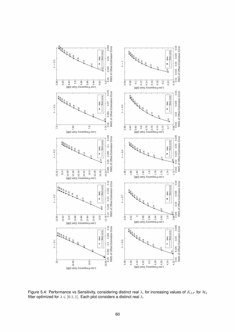
RM

S o

f Offs

et E

stim

atio

n E

rror

0.29

0.29

50.

30.

305

0.31


5

19.9

19.9

520λ=

0.1

data

fitte

d cu

rve

RM

S o

f Offs

et E

stim

atio

n E

rror

0.14

0.14

50.

150.

155

0.16


8

13.8

13.8

2

13.8

4

13.8

6

13.8

8

13.9

13.9

2

13.9

4λ=

0.2

data

fitte

d cu

rve

RM

S o

f Offs

et E

stim

atio

n E

rror

0.08

50.

090.

095

0.1

0.10

5


4

10.2

6

10.2

8

10.3

10.3

2

10.3

4

10.3

6

10.3

8

10.4

10.4

2λ=

0.3

data

fitte

d cu

rve

RM

S o

f Offs

et E

stim

atio

n E

rror

0.06

0.06

50.

070.

075

Low-Frequency Gain [dB] 7.757.

8

7.857.

9λ=

0.4

data

fitte

d cu

rve

RM

S o

f Offs

et E

stim

atio

n E

rror

0.04

0.04

50.

050.

055

Low-Frequency Gain [dB]

5.8

5.82

5.84

5.86

5.885.

9

5.92

5.94

5.96

λ=

0.5

data

fitte

d cu

rve

RM

S o

f Offs

et E

stim

atio

n E

rror

0.03

0.03

50.

040.

045


4.24

4.26

4.284.

3

4.32

4.34

4.36

4.38

λ=

0.6

data

fitte

d cu

rve

RM

S o

f Offs

et E

stim

atio

n E

rror

0.02

50.

030.

035

0.04


9

2.92

2.94

2.96

2.983

3.02

3.04

λ=

0.7

data

fitte

d cu

rve

RM

S o

f Offs

et E

stim

atio

n E

rror

0.01

50.

020.

025

0.03

0.03

5


1.74

1.76

1.781.

8

1.82

1.84

1.86

1.88

λ=

0.8

data

fitte

d cu

rve

RM

S o

f Offs

et E

stim

atio

n E

rror

0.01

50.

020.

025

0.03


7

0.72

0.74

0.76

0.780.

8

0.82

0.84

0.86

λ=

0.9

data

fitte

d cu

rve

RM

S o

f Offs

et E

stim

atio

n E

rror

0.01

0.01

50.

020.

025

0.03


4

-0.2

2

-0.2

-0.1

8

-0.1

6

-0.1

4

-0.1

2

-0.1

-0.0

8

-0.0

6λ=

1

data

fitte

d cu

rve

10

12

14

16

18

20

2224262830

10

12

14

16

18

20

2224262830

10

12

14

16

18

2022

24262830

10

12

14

16

18

20

2224

2628

30

10

12

14

16

18

20

2224

2628

30

10

12

14

16

18

20

2224

2628

30

10

12

14

16

18

20

2224

2628

30

10

12

14

16

18

20

2224

2628

30

10

12

14

16

18

2022

2426

2830

10

12

14

16

18

2022

2426

2830

Figure 5.4: Performance vs Sensitivity, considering distinct real λ, for increasing values of KLP for H2

filter optimized for λ ∈ [0.1, 1]. Each plot considers a distinct real λ.

60

Low-Pass Filter Gain KLP

10 15 20 25 30

RM

S o

f Sta

te E

stim

atio

n E

rror

0.015

0.016

0.017

0.018

0.019

0.02

0.021

0.022Min - H2

Max - H2

Max - 50% IMAEPMin - 50% IMAEP

Figure 5.5: RMS of state estimation error for increasing values of KLP ; Comparison with KF-basedapproach for 50% IMAEP design.

5.3 Performance comparison between H2 Filter and Kalman Filter

Having fully defined the design of the H2 robust filter under the actuator fault model in the previous

section, we are now in condition to provide a clear comparison, based on the system framework used

on this thesis, between the H2 filter and the Kalman filter performance. For that purpose, Fig. 5.6 shows

the RMS of state estimation error over all the uncertainty domain for both filters, in which the Kalman

filter was tuned for the nominal model 〈λ, uo〉 = 〈1, 0〉. On the other hand, the H2 filter was optimized in

the effectiveness range λ ∈ [0.1, 1].

From the mesh plot in Fig. 5.6a it is overwhelming to verify the achieved performance of the H2

filter. In an illustrative reasoning, we may state that the H2 filter RMS surface presented seems to be

flat with a negligible increase along the uncertainty domain. By contrast, the Kalman filter RMS surface

increases significantly as the fault parameters gets distant from the tuning point. However, with the aid

of the zoom-in view in Fig. 5.6b it is clear the Kalman filter actually achieves a better performance in the

tuning point and in its neighbourhood, as expected.

In a conclusive manner, the H2 filter attain approximately a 95% decrease on the RMS of the estima-

tion error for the worst-case performance with just 18% increase for the best case counter part occurring

at the nominal fault parameters point. Indeed, the results presented herein strengthen the motivation for

the study onH2 filter design and form the basis of a novel MMAE bank design discussed in the following

section.

61

(a) General View.

(b) Zoom-in view.

Figure 5.6: Performance comparison between H2 Filter and Kalman Filter.

62

5.4 Novel MMAE Bank Design

This section is focused on the MMAE filters’ bank design with the inclusion of the H2 filter. However,

before proceeding we would like to provide some remarks concerning the PPE formulation when includ-

ing an H2 filter in the MMAE bank. Some discussion may arise in how Si(k+1) shall be computed in

Eq. (4.13), which relates to the recursive law (4.15), for the conditional posterior probability evaluation.

Note that having a certain model κi matching the real plant loses significance for the H2 filter when

optimized for a certain region. Still, it was shown in Section 4.3.2 that for any admissible model the

optimal state estimation for each always yields the Kalman filter and associated steady-state residual

covariance, given by S ≡ CΣCT + R, which is constant over the whole uncertainty domain. As a con-

sequence, that value should also be applied for any H2 filter in bank independently of the optimization

range. The supporting rationale for this choice is that the recursive function implemented in the PPE

shall have a common optimal estimation reference for all filters in the bank, so that a fair comparison

between residuals is attained. Furthermore, since the innovation ν has no meaning in theH2 description

developed, we suggest the use of the residual r(k) = z(k)− Cx(k|k) for any Kalman filter present in the

bank and r(k) = z(k)−Cx(k) for the H2 filter. Based on the developed results in Section 4.1.2, similarly

it can be shown that with the use of r(k) the PPE recursive law becomes

Pi(k+1) =

(ζi(k+1)e−

12ωi(k+1)∑N


)· Pi(k) (5.34)

with ζi(k+1) ≡ 1

(2π)m2

√det Si

and ωi(k+1) ≡ ri(k+1)T Si−1

ri(k+1)

Rule (5.34) allow us to design our bank freely, which may only include Kalman filters, H2 filters or a

combination of both. Following the same reasoning, the BPM may also be redefined by

βij = ln(det Si) + Tr(S−1i Γij

)(5.35)

with Γij ≡ E{r(k)r(k)T

}as k →∞

In order to achieve a final bank design, let us first assess the RMS of the estimation error performance

of the 50% IMAEP design and compare it to the proposed H2 filter as seen in Fig. 5.8. During the

low-pass filter design in Section 5.2.3, it was concluded from Fig. 5.5 that for a filter gain KLP & 20 the

H2 filter could decrease the maximum RMS of the state estimation error to what is achieved with the

50% IMAEP approach. This is actually of paramount importance, since with a single filter we may attain

an enhanced worst-case performance, which is better than that obtained with 9 Kalman filters, over the

whole uncertainty domain. Once again, we emphasize that this result is attained at the cost of lower

performance in the KFs tuning points and their neighbourhoods.

63

Plant

KF

H2

Posterior

Probability

Evaluator

x1(k|k)

r1(k|k)

x2(k|k)

r2(k|k)

u z

x(k|k)

P (k)

S

H2 MMAE

Figure 5.7: Novel MMAE block diagram.

Figure 5.8: Performance comparison between H2 Filter and MMAE 50% IMAEP-based design.

As we are dealing with faults, assumed not to be likely to occur in regular system operation, it be-

comes relevant to have an optimal state estimation performance at the nominal condition. Therefore,

in this thesis, it is suggested the application of a combined filter structure for the MMAE bank with a

Kalman filter tuned for the nominal parameters and an H2 filter optimized in the range λ ∈ [0.1, 1], as

illustrated in Fig. 5.7. From Fig. 5.6b we can easily retain the expected state estimation performance,

whereas Fig. 5.9 provides the obtained BPM, given by Eq. (5.35), over the whole uncertainty domain.

64

(a) 3D view

(b) 2D view.

Figure 5.9: Performance comparison between H2 Filter and Kalman Filter.

65

5.5 Experiments on Simulation Environment

This section aims to test the proposed novel MMAE bank. The simulation setup follows the same

structure as that found in Section 4.4. This means that the same conditions are assumed, including the

4 distinct faults whose characterization is repeated in Table 5.1 for convenience. The fault locations on

the EIP regions for this new MMAE bank are illustrated in Fig. 5.10. The following assessment points

are defined for the present experiments:

1. Evaluate the identifiability of the models by verifying the conditional posterior probability conver-

gence to different models along with the faults incidence and removal.

2. Compare the converged models with the expected results arisen from the estimators’ bank design;

see Fig. 5.10.

Fault 1 (F#1) Fault 2 (F#2) Fault 3 (F#3) Fault 4 (F#4)λ 0.60 0.50 0.80 0.15u0 0.47 −0.90 0 0.7EIP 1 1 0 1Occurrence Time 30s-60s 90s-120s 150s-180s 210s-240s

Table 5.1: Faults description.

Figure 5.10: Faults on the EIP regions graph.

66

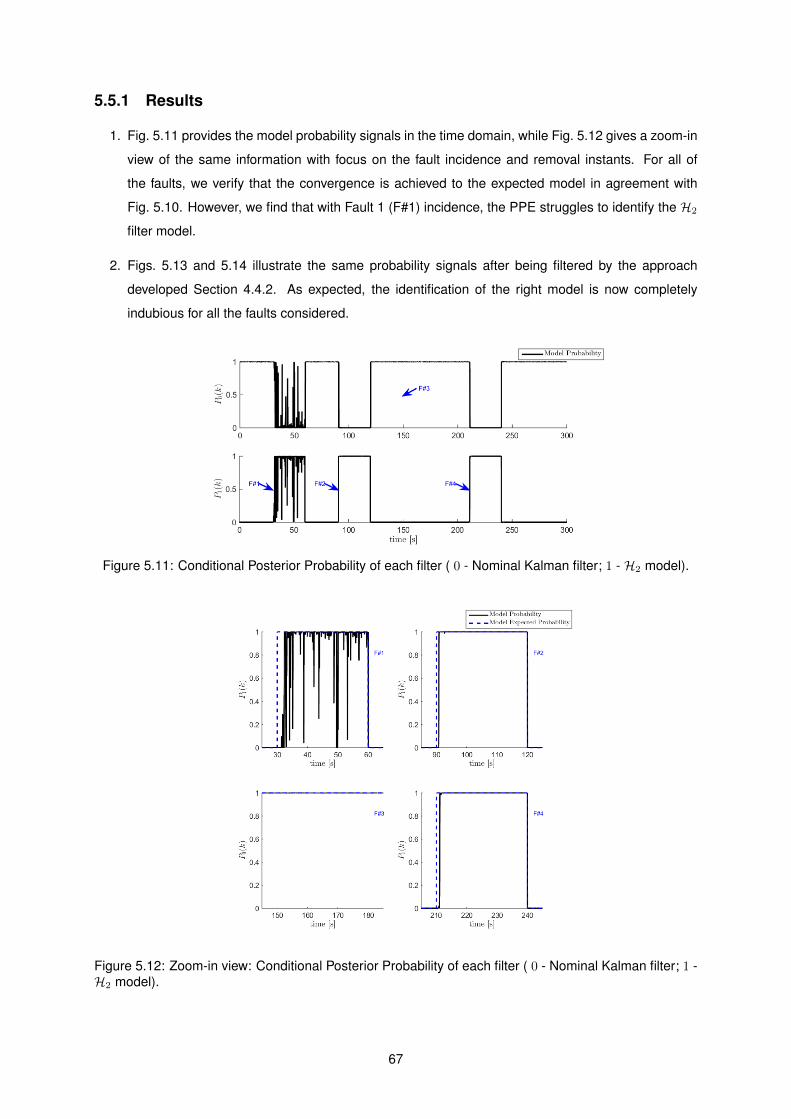
5.5.1 Results

1. Fig. 5.11 provides the model probability signals in the time domain, while Fig. 5.12 gives a zoom-in

view of the same information with focus on the fault incidence and removal instants. For all of

the faults, we verify that the convergence is achieved to the expected model in agreement with

Fig. 5.10. However, we find that with Fault 1 (F#1) incidence, the PPE struggles to identify the H2

filter model.

2. Figs. 5.13 and 5.14 illustrate the same probability signals after being filtered by the approach

developed Section 4.4.2. As expected, the identification of the right model is now completely

indubious for all the faults considered.

Figure 5.11: Conditional Posterior Probability of each filter ( 0 - Nominal Kalman filter; 1 - H2 model).

Figure 5.12: Zoom-in view: Conditional Posterior Probability of each filter ( 0 - Nominal Kalman filter; 1 -H2 model).

67

Figure 5.13: Filtered Conditional Posterior Probability of each filter ( 0 - Nominal Kalman filter; 1 - H2

model).

Figure 5.14: Zoom-in view: Filtered Conditional Posterior Probability of each model ( 0 - Nominal Kalmanfilter; 1 - H2 filter).

Comments on the Results

• The novel MMAE bank, built upon the application of a nominal Kalman filter in combination with

a H2 filter, optimized in the effectiveness parameter uncertainty domain, showed an acceptable

performance in terms of model identification considering the EIP regions obtained.

• Significant oscillations are witnessed on the original probability signals during Fault 1 (F#1) in-

cidence. However, after implementing the second filtering stage all probability signals become

smoother and clearly identify the expected model without false positives.

• These simulation results illustrate that the same level of worst-case state estimation performance

is achievable with just two filters comparing to the 9 required in Section 4.4.

68

Chapter 6

Conclusions and Future Work

6.1 Conclusions

This thesis comprehended the study of multiple-model estimation methods applied to fault detection

and isolation of linear dynamical systems. The paramount importance of safety and reliability of con-

trolled systems, namely critical systems, and the accumulated experience at the Institute for System and

Robotics (ISR) by other researchers on this methodology motivated this thesis and specific approach.

By developing a MMAE architecture, the goal was set to identify the working regime of the plant leading

to the detection of faults and identification of the operating region, which is determined by where the fault

parameters lie in a known uncertainty domain. By developing the research based on MMAE an inherent

focus of study was the accomplishment of a high performance state estimation, despite the uncertainty

regime that stemmed from the faults occurrence.

The problem at hand was divided in two stages. Initially, a classic MMAE methodology based on

Kalman filters was developed using a performance-based design for the bank. This permitted an intu-

itive determination of the filters’ tuning point and, thus, the size of the bank. Considering the developed

general actuator fault model, the design process was held in a bi-dimensional uncertainty domain, which

accounted for an effectiveness and offset fault parameters. The computational simulations performed

revealed that the developed system could effectively track the change of the working regime by conver-

gence to a different filter, depending on the localization of the fault. However, if the fault was located in

the nominal EIP region, a probability transition was no longer observed, as expected.

The performance-based design of the prequel strategy required the use of 9 KFs just for the monitor-

ing of a single actuator, becoming computationally complex for real applications. This fact motivated the

second addressed technique, which included a novel MMAE bank design in a combination of Kalman

and robust H2 filters. At this point the goal was set to the reduction of filters in the bank, while preserv-

ing the state estimation performance previously attained. The study of the latter filters was challenging

due to the interest in coping with a state estimation optimization in a polyhedral bounded domain and,

69

simultaneously, account for the bias on the dynamics resultant from the offset fault parameter. With an

equivalent performance, the outcome of this research was a bank size reduction to just 2 filters including

a nominal Kalman filter and a robust H2 filter, optimized over the whole uncertainty domain defined by

the faults’ model.

Due to the high oscillatory behaviour of the conditional probability signals in both approaches, an

independent filtering stage was also developed. The rationale behind the algorithm created was to at-

tribute cumulative scores to the models depending on their probability at every instant. This way, the

probability 1 was directly given to the first ranked filter. The result was a well-defined identification of the

models with smoother probability sequences, turning the FDI scheme specially suitable for reconfigura-

tion methods alike MMAC.

To conclude, it should be highlighted that despite the effective convergence to distinct models in both

approaches developed, the multiple-model strategies alone may fall behind in what could be expected

from a FDI scheme in terms of detection performance. Namely when the faults are located inside the

nominal EIP region. A key for this drawback could be to add several filters in the neighbourhoods of the

nominal model, but that would result in a very large bank that possibly could not meet the intended esti-

mation performance criterion. Still, the attained results with th developed techniques for multiple-model

performance-based design can not be disregarded. Particularly, the state estimation performance with

the proposed MMAE bank design, based on H2 filters, is indicative of the potentialities of this method to

any application involving plant uncertainty constraints.

6.2 Future Work

After the last six months of research which resulted in this thesis, several topics in the scope of the

study undertaken were left for future developments. Some of those are now highlighted.

Fault parameters identification In the previous section, the drawbacks on fault detection performance

from the MMAE system were emphasized. However, the possibility of guaranteeing a high level of

estimation performance under a significant plant uncertainty, and at a minimized computational cost,

motivates the search for a fault parameter identification scheme that could work in parallel or integrated

in the developed MMAE architecture. This could be the key for an optimal strategy combining both

detection and state estimation. In fact, preliminary studies on this topic were performed during the

thesis but with low theoretical support. Therefore, it is now addressed for future development.

Real scenario experiments After having completed a rather consolidated verification of the methods

developed in a simulated environment, the natural step afterwards would be to execute trials on a real

70

scenario. That would allow the validation of the method and strengthen the potentialities of the strategies

designed.

Extension to sensor and component faults The thesis was focused on actuator fault detection and

isolation. Nevertheless, the architectures designed are widely general and, thus, can easily be extended

to other types of faults, namely sensor and component faults. Note that one of the most claimed advan-

tages of the MMAE is the ease of inclusion and modelling of both additive and multiplicative faults.

H∞ and H2/H∞ synthesis With the research undertaken it was proven that other types of filters,

besides the classical ones, may be integrated in a MMAE scheme. Promising results are found in

reviewed literature comprising the application of H∞ estimators or in a combined synthesis H2/H∞.

Therefore, it would be deeply interesting to assess the applicability of these filters under the scope of

robust fault diagnosis.

71

72

References

[1] J. D. Cornelius, J. S. Orr, I. Barshi, and I. C. Statler. A Comprehensive Analysis of the X-15 Flight 3-65 Accident.

Technical Report October, National Aeronautics and Space Administration (NASA), Langley Research Center,

2014.

[2] P. W. Merlin. Michael Adams: Remembering a Fallen Hero, 2004. http://www.nasa.gov/centers/dryden/news/X-

Press/stories/2004/073004/ppl_adams_prt.htm.

[3] NTSB. Loss of Control and Impact with Pacific Ocean Alaska Airlines Flight 261. Technical report, National

Transportation Safety Board (NTSB), 2000.

[4] AAIC. Final Report Aircraft Accident Investigation Copterline OY Sikorsky S-76C+. Technical report, Aircraft

Accident Investigation Commission Ministry of Economic Affairs and Communications Estonia, 2008.

[5] R. V. Beard. Failure accomodation in linear systems through self-reorganization. PhD thesis, Massachusetts

Institute of Technology, 1971.

[6] R. Isermann and P. Ballé. Trends in the application of model-based fault detection and diagnosis of technical

processes. In Control Engineering Practice, volume 5, pages 709–719, 1997. ISBN 0967-0661. doi: 10.1016/

S0967-0661(97)00053-1.

[7] I. Hwang, S. Kim, Y. Kim, and C. E. Seah. A survey of fault detection, isolation, and reconfiguration methods.

IEEE Transactions on Control Systems Technology, 18(3):636–653, 2010. ISSN 10636536.

[8] J. Chen. Robust Residual Generation for Model-Based Fault Diagnosis of Dynamic Systems. PhD thesis,

University of York, UK, 1995.

[9] R. Hallouzi. Multiple-Model Based Diagnosis for Adaptive Fault-Tolerant Control. PhD thesis, Technical Uni-

versity of Delft, 2008.

[10] P. M. Frank. Enhancement of robustness in observer-based fault detection. International Journal of Control,

59(4):955–981, apr 1994. ISSN 0020-7179. doi: 10.1080/00207179408923112.

[11] R. Mehra and J. Peschon. An innovations approach to fault detection and diagnosis in dynamic systems.

Automatica, 7(5):637–640, sep 1971. ISSN 00051098. doi: 10.1016/0005-1098(71)90028-8.

[12] P. M. Frank. Fault diagnosis in dynamic systems using analytical and knowledge-based redundancy. Automat-

ica, 26(3):459–474, may 1990. ISSN 00051098. doi: 10.1016/0005-1098(90)90018-D.

[13] M. Visinsky, J. Cavallaro, and I. Walker. Robotic fault detection and fault tolerance: A survey. Reliability

Engineering & System Safety, 46(2):139–158, jan 1994. ISSN 09518320. doi: 10.1016/0951-8320(94)90132-

5.

73

[14] R. Isermann. Model-based fault-detection and diagnosis – status and applications. Annual Reviews in Control,

29(1):71–85, jan 2005. ISSN 13675788. doi: 10.1016/j.arcontrol.2004.12.002.

[15] R. Isermann. Fault-Diagnosis Systems. Springer Berlin Heidelberg, Berlin, Heidelberg, 2006. ISBN 978-3-

540-24112-6. doi: 10.1007/3-540-30368-5.

[16] J. Chen and R. J. Patton. Robust model-based fault diagnosis for dynamic systems, volume 11 of Kluwer

International Series on Asian Studies in Computer and Information Science. Kluwer Academic Publishers,

1999. ISBN 0792384113. doi: 10.1002/rnc.615.

[17] A. Xu and Q. Zhang. Nonlinear system fault diagnosis based on adaptive estimation. Automatica, 40(7):

1181–1193, jul 2004. ISSN 00051098. doi: 10.1016/j.automatica.2004.02.018.

[18] S. Narasimhan, P. Vachhani, and R. Rengaswamy. New nonlinear residual feedback observer for fault diagnosis

in nonlinear systems. Automatica, 44(9):2222–2229, sep 2008. ISSN 00051098. doi: 10.1016/j.automatica.

2007.12.020.

[19] X. Zhang, M. M. Polycarpou, and T. Parisini. Fault diagnosis of a class of nonlinear uncertain systems with

Lipschitz nonlinearities using adaptive estimation. Automatica, 46(2):290–299, feb 2010. ISSN 00051098. doi:

10.1016/j.automatica.2009.11.014.

[20] W. Reinelt and C. Lundquist. Observer based sensor monitoring in an active front steering system using explicit

sensor failure mo. In World Congress, volume 16, page 1246, jul 2005. ISBN 978-3-902661-75-3.

[21] A. Okatan, C. Hajiyev, and U. Hajiyeva. Fault detection in sensor information fusion Kalman filter. AEU -

International Journal of Electronics and Communications, 63(9):762–768, sep 2009. ISSN 14348411. doi:

10.1016/j.aeue.2008.06.003.

[22] G. Heredia and A. Ollero. Sensor fault detection in small autonomous helicopters using observer/Kalman

filter identification. In 2009 IEEE International Conference on Mechatronics, pages 1–6. IEEE, 2009. ISBN

978-1-4244-4194-5. doi: 10.1109/ICMECH.2009.4957236.

[23] D. Wang and K.-Y. Lum. Adaptive unknown input observer approach for aircraft actuator fault detection and

isolation. International Journal of Adaptive Control and Signal Processing, 21(1):31–48, feb 2007. ISSN

08906327. doi: 10.1002/acs.936.

[24] M. A. Demetriou. Using unknown input observers for robust adaptive fault detection in vector second-order

systems. Mechanical Systems and Signal Processing, 19(2):291–309, mar 2005. ISSN 08883270. doi:

10.1016/j.ymssp.2004.02.002.

[25] R. J. Patton. Robust Fault Detection Using Eigenstructure Assignment. Proc. IMACS World Congr. Math.

Model. Sci. Comput., pages 431–433, 1988.

[26] R. J. Patton and J. Chen. On eigenstructure assignment for robust fault diagnosis. International Jour-

nal of Robust and Nonlinear Control, 10(14):1193–1208, dec 2000. ISSN 1049-8923. doi: 10.1002/1099-

1239(20001215)10:14<1193::AID-RNC523>3.0.CO;2-R.

[27] P. S. Maybeck. Multiple Model Adaptive Algorithms for Detecting and Compensating Sensor and Actuator /

Surface Failures in Aircraft Flight Control Systems -. International Journal of Robust and Nonlinear Control,

1070:1051–1070, 1999.

74

[28] T. E. Menke and P. S. Maybeck. Sensor/actuator failure detection in the Vista F-16 by multiple model adap-

tive estimation. IEEE Transactions on Aerospace and Electronic Systems, 31(4):1218–1229, 1995. ISSN

00189251. doi: 10.1109/7.464346.

[29] J. Ru and X. R. Li. Variable-structure multiple-model approach to fault detection, identification, and estimation.

IEEE Transactions on Control Systems Technology, 16(5):1029–1038, 2008. ISSN 10636536. doi: 10.1109/

TCST.2007.916318.

[30] G. Jacques and J. Ducard. Fault-Tolerant Flight Control and Guidance Systems for a Small Unmanned Aerial

Vehicle. PhD thesis, ETH Zurich, 2007.

[31] M. Efe and D. P. Atherton. The IMM approach to the fault detection problem. 1997.

[32] Y. Zhang and X. Li. Detection and diagnosis of sensor and actuator failures using IMM estimator. IEEE

Transactions on Aerospace and Electronic Systems, 34(4):1293–1313, 1998. ISSN 00189251. doi: 10.1109/

7.722715.

[33] Y. Zhang and J. I. N. Jiang. Integrated active fault-tolerant control using IMM approach. IEEE Transactions on

Aerospace and Electronic Systems, 37(4):1221–1235, 2001. ISSN 00189251. doi: 10.1109/7.976961.

[34] A. Ray and R. Luck. An introduction to sensor signal validation in redundant measurement systems. IEEE

Control Systems, 11(2):44–49, feb 1991. ISSN 1066-033X. doi: 10.1109/37.67675.

[35] E. Chow and A. Willsky. Analytical redundancy and the design of robust failure detection systems. IEEE Trans-

actions on Automatic Control, 29(7):603–614, jul 1984. ISSN 0018-9286. doi: 10.1109/TAC.1984.1103593.

[36] W. E. Vander Velder and M.-A. Massoumnia. Generating parity relations for detecting and identifying control

system component failures. Journal of Guidance, Control, and Dynamics, 11(1):60–65, jan 1988. ISSN 0731-

5090. doi: 10.2514/3.20270.

[37] R. Isermann. Estimation of physical parameters for dynamic processes with application to an industrial robot.

In [1991 Proceedings] 6th Mediterranean Electrotechnical Conference, pages 12–17. IEEE. ISBN 0-87942-

655-1. doi: 10.1109/MELCON.1991.161769.

[38] R. Isermann. Fault diagnosis of machines via parameter estimation and knowledge processing—Tutorial paper.

Automatica, 29(4):815–835, jul 1993. ISSN 00051098. doi: 10.1016/0005-1098(93)90088-B.

[39] A. Emami-Naeini, M. Akhter, and S. Rock. Effect of model uncertainty on failure detection: the threshold

selector. IEEE Transactions on Automatic Control, 33(12):1106–1115, dec 1988. ISSN 0018-9286. doi:

10.1109/9.14432.

[40] R. J. Patton, P. M. Frank, and R. N. Clarke. Fault diagnosis in dynamic systems: theory and application.

Prentice-Hall, Inc., oct 1989. ISBN 0-13-308263-6.

[41] A. Hashemi and P. Pisu. Adaptive threshold-based fault detection and isolation for automotive electrical sys-

tems. In 2011 9th World Congress on Intelligent Control and Automation, pages 1013–1018. IEEE, jun 2011.

ISBN 978-1-61284-698-9. doi: 10.1109/WCICA.2011.5970668.

[42] S.-A. Raka and C. Combastel. Fault detection based on robust adaptive thresholds: A dynamic interval ap-

proach. Annual Reviews in Control, 37(1):119–128, apr 2013. ISSN 13675788. doi: 10.1016/j.arcontrol.2013.

04.001.

75

[43] S. Fekri, M. Athans, and A. Pascoal. Issues, progress and new results in robust adaptive control. International

Journal of Adaptive Control and Signal Processing, 20(10):519–579, dec 2006. ISSN 08906327. doi: 10.1002/

acs.912.

[44] V. Hassani, A. P. Aguiar, M. Pascoal, and M. Athans. A Performance Based Model-Set Design Strategy for

Multiple Model Adaptive Estimation. In Control Conference (ECC), 2009 European, pages 4516–4521, 2009.

ISBN 9789633113691. doi: 10.1109/CDC.2009.5399806.

[45] V. Hassani, A. P. Aguiar, M. Athans, and A. M. Pascoal. Multiple Model Adaptive Estimation and model iden-

tification usign a Minimum Energy criterion. In American Control Conference (ACC), pages 518–523, 2009.

ISBN 978-1-4244-4523-3. doi: 10.1109/ACC.2009.5160446.

[46] T. Gaspar and P. Oliveira. Single Pan and Tilt Camera Indoor Positioning and Tracking System. European

Journal of Control, 17(4):414–428, 2011. ISSN 09473580. doi: 10.3166/ejc.17.414-428.

[47] A. P. Aguiar. Multiple-model adaptive estimators: Open problems and future directions. In Control Conference

(ECC), 2007 European, pages 5544–5545, 2007.

[48] V. Hassani, A. Pascoal, and A. Aguiar. Multiple Model Adaptive Estimation for Open Loop Unstable Plants.

Proc. ECC’13 - European Control Conference, pages 1621–1626, 2013.

[49] P. Rosa. Multiple-model adaptive control of uncertain LPV systems. PhD thesis, PhD thesis, Instituto Superior

T{é}cnico, Lisbon, Portugal, 2011.

[50] P. Rosa, T. Simao, J. M. Lemos, and C. Silvestre. Multiple-model adaptive control of an air heating fan using

set-valued observers. In Control & Automation (MED), 2012 20th Mediterranean Conference on, pages 469–

474. IEEE, 2012.

[51] J. Doyle, B. Francis, and A. Tannenbaum. Feedback Control Theory. Design, 134(6):219, 1990. ISSN

00223395. doi: 10.1016/0005-1098(86)90018-X.

[52] M. I. Ribeiro. Gaussian probability density functions: Properties and error characterization. Institute for Sys-

tems and Robotics, Technical Report, (February):1–30, 2004.

[53] M. Mulder. Lecture Notes: Stochastic Aerospace Systems AE4304, 2013.

[54] M. I. Ribeiro. Kalman and Extended Kalman Filters : Concept , Derivation and Properties. Technical report,

Institute for Systems and Robotics Lisboa Portugal, 2004.

[55] J. C. Geromel, J. Bernussou, G. Garcia, and M. C. de Oliveira. H2 and H∞ robust filtering for discrete-time

linear systems. Proceedings of the 37th IEEE Conference on Decision and Control (CDC), pages 632–637,

1998.

[56] S. Boyd, L. El Ghaoui, E. Feron, and V. Balakrishnan. Linear Matrix Inequalities in System and Control Theory,

volume 15. 1994. ISBN 089871334X. doi: 10.1109/TAC.1997.557595.

[57] C. W. Scherer and S. Weiland. Linear Matrix Inequalities in Control. Lecture Notes, Dutch Institute for Systems

and Control, Delft, The Netherlands, 2000.

[58] M. de Oliveira. Lecture Notes: Linear Control Design MAE 280B, 2013.

76

[59] R. E. Kalman. A New Approach to Linear Filtering and Prediction Problems. Journal of Basic Engineering, 82

(1):35, 1960. ISSN 00219223. doi: 10.1115/1.3662552.

[60] J. J. M. Rodrigues. Optimal state estimation of LTI systems via LMI optimization. ISR (internal report).

[61] B. D. O. Anderson and J. B. Moore. Optimal Filtering. Prentice-Hall, 1979.

[62] G. Welch and G. Bishop. An Introduction to the Kalman Filter. In Practice, 7(1):1–16, 2006. ISSN 10069313.

[63] M. Athans and C.-B. Chang. Adaptive Estimation and Parameter Identification Using Multiple Model Estimation

Algorithm. Technical report, Massachussetts Institute of Technology Lincoln Lab., 1976.

[64] M. Athans. Lecture notes: Multiple-Model Adaptive Estimation (MMAE), 2001.

[65] Y. Baram. Information, Consistent Estimation and Dynamic System Identification. PhD thesis, Massachusetts

Institute of Technology, 1976.

[66] Y. Baram and N. R. Sandell. An information theoretic approach to dynamical systems modeling and identi-

fication. In Decision and Control including the 16th Symposium on Adaptive Processes and A Special Sym-

posium on Fuzzy Set Theory and Applications, 1977 IEEE Conference on, pages 1113–1118, 1977. doi:

10.1109/CDC.1977.271737.

[67] P. S. Maybeck and R. D. Stevens. Reconfigurable flight control via multiple model adaptive control methods.

IEEE Transactions on Aerospace and Electronic Systems, 27(3):470–480, may 1991. ISSN 00189251. doi:

10.1109/7.81428.

[68] O. Ahmet. Wind Turbine Fault Detection Using Counter-Based Residual Thresholding. IFAC Proceedings

Volumes (IFAC-PapersOnline), 18(PART 1):8289–8294, 2011. ISSN 14746670. doi: 10.3182/20110828-6-IT-

1002.01758.

[69] J. C. Geromel. Optimal linear filtering under parameter uncertainty. IEEE Transactions on Signal Processing,

47(1), 1999. ISSN 1053-587X. doi: 10.1109/78.738249.

[70] J. C. Geromel, P. L. D. Peres, and J. Bernussou. On a convex parameter space method for linear control design

of uncertain systems. SIAM Journal on Control and Optimization, 29(2):381–402, 1991.

[71] E. Sariyildiz and K. Ohnishi. Performance and robustness trade-off in disturbance observer design. In Industrial

Electronics Society, IECON 2013 - 39th Annual Conference of the IEEE, pages 3681–3686, 2013. ISBN 1553-

572X VO -. doi: 10.1109/IECON.2013.6699721.

[72] O. Garpinger, T. Hägglund, and K. J. Åström. Performance and robustness trade-offs in PID control. Journal

of Process Control, 24(5):568–577, may 2014. ISSN 09591524. doi: 10.1016/j.jprocont.2014.02.020.

[73] R. Hess. Analytical Assessment of Performance, Handling Qualities, and Added Dynamics in Rotorcraft Flight

Control. IEEE Transactions on Systems, Man, and Cybernetics - Part A: Systems and Humans, 39(1):262–271,

2009. ISSN 1083-4427. doi: 10.1109/TSMCA.2008.2007943.

77

78

Appendix A

Experiments: Helicopter Model

In this appendix the system model example which was applied during the simulations is presented.

This model which is of an Helicopter is directly borrowed from [73]. In that reference three sets of

nominal vehicle dynamics are indicated from where Case 1 was selected. No emphasis is given upon

the linearization procedure since it is out of the scope of the present thesis. We stress that the selected

system provides only one possible applicable linearized model to the methodologies developed during

the research, which were not specifically designed or adapted to it. That being said, consider a state-

space vehicle model given by

x = Ax +Bu (A.1)

with

x =[u w q θ v p r ψ

]Tu =

[δB δC δA δP

]TThe system and input matrices, respectively given by A and B, are in the form

A =

Xu 0 0 −g 0 0 0 0

0 Zw U0 −g 0 0 0 0

0 0 Mq Mθ 0 Mp 0 0

0 0 1 0 0 0 0 0

0 0 0 0 Yv 0 −U0 g

0 0 Lq 0 0 Lp 0 Lψ

0 0 0 0 0 0 Nr 0

0 0 0 0 0 1 0 0

(A.2a)

79

B =

0 0 0 0

0 ZδC 0 0

MδB 0 MδA 0

0 0 0 0

0 0 0 0

LδB 0 LδA 0

0 0 0 NδP

0 0 0 0

(A.2b)

The values for all the stability derivatives in A and B matrices are given in Table A.1.

Derivative ValueXu

1sec −0.01

Zw1

sec −1.00Mq

1sec −3.00

Mθ1

rad-sec2 0.00Mp

1sec 0.00

Yv1

sec −0.02Lq

1sec 0.00

Lp1

sec −5.00Lψ

1rad-sec2 0.00

ZδCft

rad-sec2 −7.00MδB

1rad-sec2 −0.70

MδA1

rad-sec2 0.00LδB

1rad-sec2 0.00

LδA1

rad-sec2 2.00LδP

1rad-sec2 −3.00

Table A.1: Stability derivative values for the helicopter state-space model.

The gravity acceleration constant was set to g = 9.81 m/s2. Before running the intended simulations,

a discretization step was performed with a zero-order hold method at a sampling time Ts = 0.02 s,

defined to be lower than the smallest time-constant of the system.

80

Fault Detection and Isolation for Linear Dynamical Systems · Fault Detection and Isolation for Linear Dynamical Systems ... com aplicação na área de deteção e isolamento de

Documents