Fault Detection And Diagnosis For Air Conditioners And Heat ...

Purdue UniversityPurdue e-Pubs

Open Access Dissertations Theses and Dissertations

Fall 2013

Fault Detection And Diagnosis For AirConditioners And Heat Pumps Based On VirtualSensorsWoohyun KimPurdue University

Follow this and additional works at: https://docs.lib.purdue.edu/open_access_dissertations

Part of the Mechanical Engineering Commons

This document has been made available through Purdue e-Pubs, a service of the Purdue University Libraries. Please contact [email protected] foradditional information.

Recommended CitationKim, Woohyun, "Fault Detection And Diagnosis For Air Conditioners And Heat Pumps Based On Virtual Sensors" (2013). OpenAccess Dissertations. 153.https://docs.lib.purdue.edu/open_access_dissertations/153

https://docs.lib.purdue.edu?utm_source=docs.lib.purdue.edu%2Fopen_access_dissertations%2F153&utm_medium=PDF&utm_campaign=PDFCoverPages

https://docs.lib.purdue.edu/open_access_dissertations?utm_source=docs.lib.purdue.edu%2Fopen_access_dissertations%2F153&utm_medium=PDF&utm_campaign=PDFCoverPages

https://docs.lib.purdue.edu/etd?utm_source=docs.lib.purdue.edu%2Fopen_access_dissertations%2F153&utm_medium=PDF&utm_campaign=PDFCoverPages

https://docs.lib.purdue.edu/open_access_dissertations?utm_source=docs.lib.purdue.edu%2Fopen_access_dissertations%2F153&utm_medium=PDF&utm_campaign=PDFCoverPages

http://network.bepress.com/hgg/discipline/293?utm_source=docs.lib.purdue.edu%2Fopen_access_dissertations%2F153&utm_medium=PDF&utm_campaign=PDFCoverPages

https://docs.lib.purdue.edu/open_access_dissertations/153?utm_source=docs.lib.purdue.edu%2Fopen_access_dissertations%2F153&utm_medium=PDF&utm_campaign=PDFCoverPages

Graduate School ETD Form 9 (Revised 12/07)

PURDUE UNIVERSITY GRADUATE SCHOOL

Thesis/Dissertation Acceptance

This is to certify that the thesis/dissertation prepared

By

Entitled

For the degree of

Is approved by the final examining committee:

Chair

To the best of my knowledge and as understood by the student in the Research Integrity and Copyright Disclaimer (Graduate School Form 20), this thesis/dissertation adheres to the provisions of Purdue University’s “Policy on Integrity in Research” and the use of copyrighted material.

Approved by Major Professor(s): ____________________________________

____________________________________

Approved by: Head of the Graduate Program Date

Woohyun Kim

Fault Detection and Diagnosis for Air Conditioners and Heat Pumps based on Virtual Sensors

Doctor of Philosophy

James E. Braun

Eckhard Groll

W. Travis Horton

Haorong Li

James E. Braun

David Anderson 08/26/2013

i

FAULT DETECTION AND DIAGNOSIS FOR AIR CONDITIONERS AND HEAT

PUMPS BASED ON VIRTUAL SENSORS

A Dissertation

Submitted to the Faculty

of

Purdue University

by

Woohyun Kim

In Partial Fulfillment of the

Requirements for the Degree

of

Doctor of Philosophy

December 2013

Purdue University

West Lafayette, Indiana

ii

For my parents who taught me to value the gift of education

and my wife and Coco who showed me to value the power of love.

iii

ACKNOWLEDGEMENTS

With sincere reverence, the author would like to thank Professor James E. Braun for his

continuous trust and encouragement and thoughtful criticism throughout the years.

Without his guidance and patience, this research would not have been possible. The

author also likes to thank Professor Eckhard Groll, Professor Travis W. Horton, and

Professor Haorong Li for their feedback and warm support.

iv

TABLE OF CONTENTS

Page

LIST OF TABLES ............................................................................................................. xi

LIST OF FIGURES ......................................................................................................... xiii

NOMENCLATURE ...................................................................................................... xxiv

ABSTRACT ......................................................................................................... xxxii

CHAPTER 1. INTRODUCTION ................................................................................. 1

1.1 Background and Motivation ...................................................................... 1

1.1.1 Potential for FDD Applied to Air Conditioners and Heat Pump

Systems ............................................................................................................ 1

1.1.2 Earlier FDD Approaches for Air Conditioners and Heat Pump

Systems ............................................................................................................ 2

1.1.3 Summary and Limitations of Earlier FDD Approaches ..................... 9

1.1.4 Need for Economic Assessment in Making Recommendations ...... 10

1.2 Review of Virtual Sensors....................................................................... 12

1.2.1 Benefits of Virtual Sensors .............................................................. 13

1.2.2 General Steps for Developing Virtual Sensors ................................ 14

1.2.3 Overview of Virtual Sensor Developments in Other Fields ............ 15

1.2.3.1 Virtual Sensing in Automobiles .......................................................... 16

1.2.3.2 Virtual Sensing in Control Systems..................................................... 17

1.2.4 Review of Virtual Sensors for HVAC&R ........................................ 18

1.3 Literature Review for Impact of Faults ................................................... 19

1.3.1 Literature Review for Refrigerant Charge Faults ............................. 20

1.3.2 Literature Review for Heat Exchanger Fouling ............................... 21

1.4 Thesis Objectives .................................................................................... 22

v

Page

CHAPTER 2. IMPACT OF FAULTS ON PERFORMANCE AND COSTS ........... 25

2.1 Data Reduction for the Impact of Fault on Performance ........................ 26

2.2 System Descriptions and Test Conditions ............................................... 28

2.2.1 System Descriptions and Test Conditions for Refrigerant Charge .. 28

2.2.2 System Descriptions and Test Conditions for Fouling ..................... 29

2.3 Impact of Refrigerant Charge and Heat Exchanger Fouling on

Performanc e ............................................................................................................... 31

2.3.1 Impact of Refrigerant Charge on Performance ................................ 31

2.3.1.1 Impact of Refrigerant Charge for System with a Constant-speed

Compressor ........................................................................................................... 31

2.3.1.2 Impact of Refrigerant Charge for System with Variable-speed

Compressor ........................................................................................................... 33

2.3.2 Impact of Fouling on Performance ................................................... 36

2.3.2.1 Impact of Evaporator Fouling on Performance ................................... 37

2.3.2.2 Impact of Condenser Fouling on Performance .................................... 38

2.4 Impact of Refrigerant Charge and Heat Exchanger Fouling on Costs .... 40

2.4.1 Impact of Refrigerant Charge on Energy Costs ............................... 41

2.4.2 Impact of Evaporator Fouling on Energy Costs ............................... 43

2.4.3 Impact of Condenser Fouling on Energy Costs ............................... 44

2.5 Summary ................................................................................................. 45

CHAPTER 3. EXTENSION, DEVELOPMENT AND ASSESSMENT OF

VIRTUAL SENSORS FOR VARIABLE-SPEED COMPRESSORS ............................. 47

3.1 Extension of Virtual Refrigerant Charge (VRC) Sensor for Variable-

Speed Compressors ....................................................................................................... 47

3.1.1 Original VRC Sensor for Fixed-Speed Compressor ........................ 49

3.1.2 Modified VRC Sensor for Variable-Speed Compressor .................. 53

3.1.3 Performance of VRC sensor for Cooling Equipment with Variable-

Speed Compressor .................................................................................................... 57

vi

Page

3.1.3.1 System descriptions and test conditions .............................................. 57

3.1.3.2 Evaluation of VRC Sensor for a Air Conditioner Equipment with

Variable-Speed Compressors ................................................................................ 59

3.1.4 Performance of the VRC sensor for Air conditioner Equipment

with Fixed-Speed Compressors ................................................................................ 62

3.1.4.1 System Descriptions and Test Conditions for Air Conditioner

Equipment with Fixed-Speed Compressors .......................................................... 62

3.1.4.2 Evaluation of VRC Sensor for A/C Equipment with Fixed-Speed

Compressors .......................................................................................................... 64

3.1.5 Performance of the VRC Sensor for Heat Pump Systems with

Variable-speed Compressors..................................................................................... 68

3.1.5.1 System descriptions and test conditions for heat pump systems with

variable-speed compressors .................................................................................. 68

3.1.5.2 Sensor Locations for the VRC Sensor Applied to Heat Pump Systems ..

............................................................................................................. 69

3.1.5.3 Evaluation of VRC sensor for Heat Pump Systems with Variable-

Speed Compressor ................................................................................................ 74

3.1.6 Comparison with Manufacturer’s Charging Method ....................... 77

3.1.7 Summary of the VRC Sensor ........................................................... 79

3.2 Development of Virtual Refrigerant Mass Flow (VRMF) and Virtual

Compressor Power (VCP) Sensor for Variable-Speed Compressors ........................... 81

3.2.1 Specification and Test Condition ..................................................... 82

3.2.2 Virtual Sensor Modeling for Systems with Variable Speed

Compressors .......................................................................................................... 83

3.2.2.1 Refrigerant Volumetric Flow Rate and Power Input at Rated

Frequency ............................................................................................................. 83

3.2.2.2 Correction Modeling at Different Frequencies .................................... 84

vii

Page

3.2.3 Performance of Virtual Sensors for Systems with Variable-Speed

Compressors .......................................................................................................... 87

3.2.3.1 Evaluation of Virtual Sensors for Systems with Variable-Speed

Compressors .......................................................................................................... 87

3.2.3.2 Prediction of Compressor Frequency .................................................. 89

3.2.4 Summary for the VRMF and VCP Sensors ..................................... 91

CHAPTER 4. DEVELOPMENT AND ASSESSMENT OF ALTERNATIVE

VIRTUAL SENSORS ...................................................................................................... 93

4.1 Development and Assessment of Virtual Refrigerant Mass Flow

(VRMF) Sensors ........................................................................................................... 93

4.1.1 System Descriptions and Test Conditions ........................................ 93

4.1.2 VRMF sensor I based on Compressor Flow Map ............................ 95

4.1.2.1 Development of VRMF Sensor I ......................................................... 95

4.1.2.2 Performance of VRMF Sensor I .......................................................... 96

4.1.3 VRMF sensor II based on Compressor Energy Balance .................. 99

4.1.3.1 Development of VRMF Sensor II ....................................................... 99

4.1.3.2 Performance of VRMF Sensor II ....................................................... 100

4.1.4 VRMF sensor III based on Expansion Valve Model ..................... 102

4.1.4.1 Development of VRMF Sensor III for TXVs .................................... 103

4.1.4.2 Performance of VRMF Sensor III for TXVs ..................................... 106

4.1.4.3 Development of VRMF Sensor III for EEV ...................................... 108

4.1.4.4 Performance of VRMF Sensor III for EEVs ..................................... 110

4.1.5 Application of VRMF Sensors for Fault Detection and Diagnosis 113

4.1.6 Summary for Alternative VRMF Sensors ...................................... 116

4.2 Development and Assessment of a Virtual Air Flow (VAF) and

Virtual Heat Exchanger Conductance (VHXC) Sensor .............................................. 117

4.2.1 VAF and VHXC Sensors for Condensers ...................................... 117

viii

Page

4.2.1.1 Virtual Sensor for Condensers based on an Energy Balance ............ 118

4.2.1.2 Virtual Sensor for Condenser based on UA ...................................... 120

4.2.2 VAF and VHXC Sensor for Evaporator ........................................ 122

4.2.2.1 Virtual sensor for evaporators based on an energy balance .............. 123

4.2.2.2 Virtual sensor for evaporators based on UA ..................................... 124

CHAPTER 5. STRUCTURE FOR A DIAGNOSTIC DECISION SYSTEM ......... 127

5.1 Steady State Detector for Preprocessor ................................................. 130

5.2 Fault Detection ...................................................................................... 131

5.2.1 Bayesian Fault Detection Classifier ............................................... 131

5.2.2 Normalized Distance Detection Classifier ..................................... 136

5.3 Fault Diagnosis and Decision ................................................................ 137

5.4 Fault Detection and Diagnosis Analysis ............................................... 141

CHAPTER 6. FAULT DETECTION BASED ON VIRTUAL SENSORS FOR

LABORATORY AND FIELD TESTS .......................................................................... 149

6.1 RTU FDD Assessments using Laboratory and Field Test Data............ 150

6.1.1 System Description and Test Conditions ....................................... 150

6.1.2 Virtual Sensor Developments and Evaluations .............................. 152

6.1.2.1 VRC Sensor: Refrigerant Undercharge and Overcharge ................... 152

6.1.2.2 VCP Sensor: Compressor Power ....................................................... 158

6.1.2.3 VRMF Sensor: Refrigerant Mass Flow Rate ..................................... 159

6.1.2.4 VAF Sensor: Improper Outdoor Air Flow Rate ................................ 164

6.1.2.5 VAF Sensor: Improper Indoor Air Flow Rate ................................... 166

6.1.3 Diagnostics Performance Evaluations ............................................ 167

6.1.3.1 Diagnostics Performance Evaluation for RTU I ................................ 167

6.1.3.2 Diagnostics Performance Evaluation for RTU II .............................. 169

6.1.3.3 Diagnostics Performance Evaluation for RTU III ............................. 171

ix

Page

6.1.4 Initial Demonstration of the FDD Approach based on Virtual

Sensor ........................................................................................................ 173

6.2 DX Systems Field Testing..................................................................... 176

6.2.1 Field Fault Test Conditions and System Descriptions ................... 176

6.2.2 Virtual Sensor Development and Evaluation ................................. 177

6.2.2.1 VRC Sensor Development and Evaluation ....................................... 177

6.2.2.2 VRMF Sensor Development and Evaluation .................................... 179

6.2.2.3 VAF Sensor Development and Evaluation ........................................ 181

6.2.2.4 Initial Demonstration of Virtual Sensors for DX Systems ................ 182

6.2.3 Demonstration of the VRC and VAF sensors for the DX system .. 183

6.2.3.1 Refrigerant undercharge and overcharge for DX system 3 circuit A 183

6.2.3.2 Improper Condenser Air Flow Rate for DX System 3 Circuit A ...... 187

6.3 Embedded Automated Fault Detection and Diagnostic (AFDD)

System ............................................................................................................... 190

6.3.1 User Interface Development ........................................................... 190

6.3.2 Virtual Sensor Implementation ...................................................... 191

CHAPTER 7. COMPLETE EVALUATION, IMPLEMENTATION, AND

VALIDATION OF RTU DIAGNOSTIC PERFORMANCE......................................... 196

7.1 System Specification ............................................................................. 197

7.2 Test Conditions ..................................................................................... 199

7.2.1 Single-Fault Test Conditions .......................................................... 199

7.2.2 Multiple-Fault Test Conditions ...................................................... 201

7.2.3 Uncertainty Analysis ...................................................................... 202

7.3 Performance of Virtual Sensors for Single-Fault Laboratory Test

Results ............................................................................................................... 204

7.3.1 VRMF Sensors: Compressor Valve Leaage and Faulty

Expansion Valve ..................................................................................................... 204

7.3.2 VAF Sensors: Improper Outdoor and Indoor Air Flow Rates ....... 208

x

Page

7.3.3 VRC Sensor: Refrigerant Charge Fault .......................................... 210

7.3.4 VP Sensor: Liquid Line and/or Filter Restriction .......................... 212

7.4 Performance of Virtual Sensors for Multiple-Faults using Laboratory

Test Results ............................................................................................................... 213

7.5 FDD Method based on Virtual Sensors and Fault Impact Model ......... 219

7.6 Overall FDD System Performance Under Single-Fault Conditions ..... 230

7.7 Overall FDD System Performance under Multiple-Simultaneous Fault

Conditions ............................................................................................................... 235

7.8 Summary ............................................................................................... 242

CHAPTER 8. CONCLUSION ................................................................................. 244

8.1 Conclusion ............................................................................................. 244

8.2 Recommendations ................................................................................. 249

LIST OF REFERENCES ................................................................................................ 251

APPENDIX: PARAMETERS OF VIRTUAL SENSORS ............................................. 260

VITA ........................................................................................................... 270

xi

LIST OF TABLES

Table .............................................................................................................................. Page

Table 1.1. Summary of virtual sensors for air conditioners (Yu, Li & Braun, 2011). ...... 18

Table 1.2. Summary of fault incidence analysis. .............................................................. 20

Table 1.3. Summary of fault impact analysis. .................................................................. 20

Table 2.1. System Specifications. ..................................................................................... 29

Table 2.2. Test Conditions. ............................................................................................... 29

Table 2.3. System Specifications. ..................................................................................... 30

Table 2.4. Test Conditions. ............................................................................................... 30

Table 2.5. Bin Weather data for SEER. ............................................................................ 40

Table 3.1. Comparison between parameters based on measurements and calculation. .... 51

Table 3.2. System descriptions for existing refrigerant charge level test data. ................ 58

Table 3.3. Test conditions for cooling equipment having a variable-speed compressor. . 58

Table 3.4. System descriptions for cooling equipment with fixed-speed compressors. ... 63

Table 3.5. Test conditions for cooling equipment having a fixed-speed compressor....... 64

Table 3.6. System description for heat pump systems having a variable-speed

compressor. ....................................................................................................................... 69

Table 3.7. Test conditions for heat pump systems having a variable-speed compressor. 69

Table 3.8. Sensor locations for heat pump units in cooling mode and heating mode. ..... 74

Table 3.9. Descriptions for systems with variable-speed compressors. ........................... 83

Table 3.10. Testing conditions for systems with variable-speed compressors. ................ 83

Table 4.1. System descriptions for laboratory test data. ................................................... 95

Table 4.2. Test conditions for laboratory test data........................................................... 95

Table 5.1. Calculation of threshold for 1) Bayes classifier and 2) Normal distance

method............................................................................................................................. 142

xii

Table .............................................................................................................................. Page

Table 5.2. FDD response to compressor valve leakage based on Bayes classifier. ........ 143

Table 5.3. FDD response to 1) low refrigerant charge, 2) condenser fouling, and 3)

liquid line restriction faults based on Bayes classifier. ................................................... 144

Table 5.4. FDD response to compressor valve leakage based on simple distance

method............................................................................................................................. 145

Table 5.5. FDD response to 1) low refrigerant charge, 2) condenser fouling, and 3)

liquid line restriction faults based on simple distance method. ...................................... 145

Table 6.1. Specification of RTU system. ........................................................................ 150

Table 6.2. Testing conditions. ......................................................................................... 152

Table 6.3. System specifications of DX systems 2 & 3. ................................................. 177

Table 7.1. Specifications of the RTU system. ................................................................ 197

Table 7.2. Individual fault levels implemented in single fault condition. ...................... 201

Table 7.3. Individual fault levels implemented in multiple simultaneous fault

conditions. ....................................................................................................................... 202

Table 7.4. Independent measurement uncertainties for the RTU system. ...................... 203

Table 7.5. Uncertainties of dependent variables for the RTU system. ........................... 204

xiii

LIST OF FIGURES

Figure ............................................................................................................................. Page

Figure 1.1. Breakdown of system and FDD method used in the literature review. .......... 10

Figure 1.2. Breakdown of system actuators used in the literature review. ....................... 10

Figure 1.3. General steps for developing virtual sensors. ................................................. 15

Figure 1.4. Virtual sensors for systemized vehicle (from Yu, et al., 2011). ..................... 17

Figure 2.1. Capacity ratios for existing test data based on the refrigerant charge. ........... 32

Figure 2.2. COP ratios for existing test data based on the refrigerant charge. ................. 33

Figure 2.3. Cooling capacity ratios for system A6 based on refrigerant charge. .............. 35

Figure 2.4. Cooling COP ratios for system A6 based on refrigerant charge. ................... 35

Figure 2.5. Heating capacity ratios for system A6 based on the refrigerant charge. ........ 36

Figure 2.6. Heating COP ratios for system A6 based on the refrigerant charge. .............. 36

Figure 2.7. Capacity ratios for RTU and split air conditioner based on indoor air flow rate.

........................................................................................................................................... 38

Figure 2.8. COP ratios for RTU and split air conditioner based on indoor air flow rate. . 38

Figure 2.9. Capacity ratio based on outdoor air flow rate. ............................................... 39

Figure 2.10. COP ratio based on outdoor air flow rate. .................................................... 40

Figure 2.11. SEER ratios for all test data as a function of refrigerant charge. ................. 42

Figure 2.12. Annual cost ratios for all test data as a function of refrigerant charge. ........ 42

Figure 2.13. SEER ratios for RTU and split air conditioner based on indoor air flow rate.

........................................................................................................................................... 43

Figure 2.14. Cost ratios for RTU and Split air conditioner based on indoor air flow

rate..................................................................................................................................... 43

Figure 2.15. SEER ratios based on outdoor air flow rate. ................................................ 44

Figure 3.1. Operating states of the vapor compression cycle. .......................................... 56

xiv

Figure ............................................................................................................................. Page

Figure 3.2. Performance of VRC sensor model I based on default parameters for

cooling equipment with variable-speed compressor. ........................................................ 60

Figure 3.3. Performance of VRC sensor model II based on default parameters for

cooling equipment with variable-speed compressor. ........................................................ 61

Figure 3.4. Performance of VRC sensor model I based on tuned parameters for cooling

equipment with variable-speed compressor. ..................................................................... 61

Figure 3.5. Performance of VRC sensor model II based on tuned parameters for cooling

equipment with variable-speed compressor. ..................................................................... 62

Figure 3.6. Performance of VRC sensor model I based on simulation parameters for

cooling equipment with fixed-speed compressors. ........................................................... 65

Figure 3.7. Performance of VRC sensor model II based on simulation parameters for



equipment with fixed-speed compressors. ........................................................................ 66

Figure 3.9. Performance of VRC sensor model II based on tuned parameters for


Figure 3.10. Sensor locations of indoor unit heat exchanger for cooling and heating

mode. ................................................................................................................................. 71

Figure 3.11. Sensor locations of outdoor unit heat exchanger for cooling and heating

mode. ................................................................................................................................. 71

Figure 3.12. Comparison between evaporator saturation temperature based on pressure

measurements and based on temperature measurements for different compressor speeds

in cooling mode (OD Temp: 95F). ................................................................................... 72

Figure 3.13. Comparison between condenser saturation temperature based on pressure


in cooling mode (OD Temp: 95F). ................................................................................... 72

Figure 3.14. Comparison between evaporator saturation temperature based on pressure


in heating mode (OD Temp: 47F). .................................................................................... 73

xv

Figure ............................................................................................................................. Page

Figure 3.15. Comparison between condenser saturation temperature based on pressure


in heating mode (OD Temp: 47F). .................................................................................... 73

Figure 3.16. Performance of VRC sensor model II based on default parameters for heat

pumps. ............................................................................................................................... 76


heat pumps. ....................................................................................................................... 76

Figure 3.18. Performance of VRC sensor model II based on tuned parameters for heat

pumps. ............................................................................................................................... 77

Figure 3.19. Performance of VRC sensor model III based on tuned parameters for heat

pumps. ............................................................................................................................... 77

Figure 3.20. Refrigerant charge method based on manufacturer’s method for cooling

mode (System C-9). .......................................................................................................... 78

Figure 3.21. Performance of VRC sensor model III based on tuned parameters for cooling

mode (System C-9). .......................................................................................................... 79

Figure 3.22. Kflow in terms of evaporation temperature for different frequencies and

ambient (condensing) temperatures (system D-2). ........................................................... 86

Figure 3.23. Kinput in terms of evaporation temperature for different frequencies and

ambient (condensing) temperatures (system D-2). ........................................................... 86

Figure 3.24. Performance of VRMF sensor (mass flow rate) under no fault conditions. . 88

Figure 3.25. Performance of VRMF sensor (mass flow rate) under fault conditions. ...... 88

Figure 3.26. Performance of VCP sensor (input power) under no fault conditions. ........ 89

Figure 3.27. Performance of VCP sensor (input power) under fault conditions. ............. 89

Figure 3.28. Comparisons of predicted and measured compressor frequencies for

system D-2. ....................................................................................................................... 91

Figure 3.29. Comparisons of predicted and measured compressor frequencies for

system D-4. ....................................................................................................................... 91

xvi

Figure ............................................................................................................................. Page

Figure 4.1. Performance of VRMF sensor I based on a fixed-speed compressor map for

system E-3 under no-fault and fault conditions (RMS of sensor errors is shown for each

fault type). ......................................................................................................................... 98

Figure 4.2. Performance of VRMF sensor I based on a variable-speed compressor map

for system E-1 under no-fault and fault conditions (RMS of sensor errors is shown for

each fault type). ................................................................................................................. 98

Figure 4.3. Performance of VRMF sensor II based on an energy balance for system

E-3 under no fault and fault conditions (RMS of errors is shown for each fault type). . 101

Figure 4.4. Performance of VRMF sensor II based on an energy balance for system E-

1 under no fault and fault conditions (RMS of errors is shown for each fault type). ..... 102

Figure 4.5. Diagram of a TXV. ....................................................................................... 104

Figure 4.6. Performance of VRMF sensor III based on a TXV model for system E-3

under no-fault and fault conditions (RMS of sensor errors is shown for each fault type).

......................................................................................................................................... 107

Figure 4.7. Flow passage structure and geometric models for EEV. .............................. 109

Figure 4.8. Performance of VRMF sensor III based on EEV for system E-1 under no fault

and fault conditions (RMS of sensor errors shown for each fault type). ........................ 111

Figure 4.9. Performance of VRMF sensor III based on EEV with R410a as refrigerant

or system E-2. ................................................................................................................. 112


for system E-2. ................................................................................................................ 112

Figure 4.11. Comparison of VRMF sensor outputs for system E-3 with a compressor

flow fault. ........................................................................................................................ 114

Figure 4.12. Comparison of VRMF sensor outputs for system E-1 with a compressor

flow fault. ........................................................................................................................ 115

Figure 4.13. Comparison of VRMF sensor outputs for system E-2 (R410A) with a

compressor flow fault. .................................................................................................... 115


compressor flow fault. .................................................................................................... 116

xvii

Figure ............................................................................................................................. Page

Figure 4.15. Virtual sensor for condensers using 1) energy balance and 2) overall

condenser conductance. ................................................................................................... 118

Figure 4.16. Predicted condenser air flow from an energy balance versus expected

value for system E-3. ...................................................................................................... 120

Figure 4.17. Calculated UAcond as a function of deviation from normal charge for

system E-3. ...................................................................................................................... 122

Figure 4.18. Expected UAcond versus UAcond determined from measurements for system

......................................................................................................................................... 122

Figure 4.19. VAF sensor for evaporators using 1) energy balance and 2) overall

conductance..................................................................................................................... 123

Figure 4.20. Predicted evaporator air flow from an energy balance versus expected

value for system E-3. ...................................................................................................... 124

Figure 4.21. Calculated UAevap as a function of deviation from normal charge fo r

system E-3. ...................................................................................................................... 126

Figure 4.22. Expected UAevap versus UAevap determined from measurements fo r

system E-3. ...................................................................................................................... 126

Figure 5.1. FDD block diagram for RTUs. ..................................................................... 127

Figure 5.2. Virtual sensor classifications for air conditioners. ....................................... 129

Figure 5.3. Example of virtual sensor interactions for air conditioning equipment. ...... 130

Figure 5.4. Bayes decision rule for minimum error (w1 : no fault & w2 : fault

condition). ....................................................................................................................... 133

Figure 5.5. Overall fault interactions for air conditioning equipment. ........................... 138

Figure 5.6. Scheme for using VRMF sensors to identify compressor or expansion

valve faults. ..................................................................................................................... 142

Figure 5.7. Comparison between the virtual sensors and the expected performance

model (Capacity) for system E-3 under compressor valve leakage fault. ...................... 147

Figure 5.8 Comparison between the virtual sensors and the expected performance

model (COP) for system E-3 under compressor valve leakage fault .............................. 148

xviii

Figure ............................................................................................................................. Page

Figure 5.9. Comparison between the virtual sensors and the expected performance

model for system E-3 under other faults conditions. ...................................................... 148

Figure 6.1. Performance of VRC sensor model 3 based on tuned parameters for RTU I

laboratory data. ............................................................................................................... 153

Figure 6.2. Performance of VRC sensor model 3 based on tuned parameters for the

RTU III laboratory data. ................................................................................................. 154

Figure 6.3. Charging results based on manufacturers’ charging method for RTU II

under no heat exchanger blocking. ................................................................................. 155

Figure 6.4. Charging results based on manufacturers’ charging method for RTU II

under heat exchanger blocking. ...................................................................................... 156

Figure 6.5. Performance of VRC sensor model III based on tuned parameters for RTU

II under no condenser fouling. ........................................................................................ 157

Figure 6.6. Performance of VRC sensor model III based on tuned parameters for RTU

II under condenser fouling. ............................................................................................. 157

Figure 6.7. Performance of VCP sensors for RTU I under normal and faulty conditions.

......................................................................................................................................... 158

Figure 6.8. Performance of VCP sensors for RTU II under normal and faulty conditions.

......................................................................................................................................... 159

Figure 6.9. Performance of VCP sensor for RTU III under normal and faulty conditions.

......................................................................................................................................... 159

Figure 6.10. Performance of VRMF sensor for RTU I based on model I and II under

normal and faulty conditions. ......................................................................................... 161

Figure 6.11. Performance of VRMF sensors for RTU II based on model I and II under


Figure 6.12. Performance of VRMF sensors for RTU III based on model I and II under


Figure 6.13. Performance of VRMF sensor for RTU I based on model II and III under


xix

Figure ............................................................................................................................. Page

Figure 6.14. Performance of VRMF sensor for RTU II based on model II and III under


Figure 6.15. Performance of VRMF sensor for RTU III based on model II and III under


Figure 6.16. Performance of VAF sensor (condenser) for RTU II under normal

refrigerant charge. ........................................................................................................... 165

Figure 6.17. Performance of VAF sensor (condenser) for RTU II under different

refrigerant charge levels. ................................................................................................. 165

Figure 6.18. Predicted evaporator air flow from an energy balance versus expected

value based on fan setting for RTU III. .......................................................................... 166

Figure 6.19. Comparison between the virtual sensor and the expected performance

model for RTU system I under normal conditions. ........................................................ 168


model for RTU system I under refrigerant undercharge fault conditions. ...................... 168


model for RTU system II under condenser fouling fault conditions. ............................. 170

Figure 6.22. Comparison between thevirtual sensor and the expected performance

model for RTU system II under 90% refrigerant charge and condenser fouling fault

conditions. ....................................................................................................................... 170



conditions. ....................................................................................................................... 171



conditions. ....................................................................................................................... 171


model for RTU system III under no faults conditions. ................................................... 172


model for RTU system III under refrigerant charge faults. ............................................ 173

xx

Figure ............................................................................................................................. Page

Figure 6.27. FDD display for 75% refrigerant charge level and 0% condenser fouling

level demonstration. ........................................................................................................ 174



Figure 6.29. Condenser status of RTU system (left side: normal & right side: 50%

blocking). ........................................................................................................................ 176



Figure 6.31. VRC sensor outputs based on default parameters for DX unit 3 circuits

A & B. ............................................................................................................................. 178

Figure 6.32. VRC sensor outputs based on default parameters for DX unit 3 circuits

A & B. ............................................................................................................................. 179

Figure 6.33. VRMF sensor outputs based on an energy balance for DX unit 2 circuit A.

......................................................................................................................................... 180

Figure 6.34. Accuracy of predicted power based on compressor map for DX system 3

circuits A & B. ................................................................................................................ 181

Figure 6.35. Performance of VAF sensors based on an energy balance for DX system 3.

......................................................................................................................................... 181

Figure 6.36. Performance of the VRC, VRMF, and VAF sensors for the DX system. .. 182

Figure 6.37. Example of the virtual sensor display from a demonstration of the FDD

tool for the DX system. ................................................................................................... 183

Figure 6.38. Refrigerant charge test condition for DX system 3 circuit A. .................... 184

Figure 6.39. Performance of VRC sensors I and III with no condenser fouling (tuned

parameters based on refrigerant charge test data). .......................................................... 185

Figure 6.40. Performance of VRC sensors I and III with condenser fouling (tuned

parameters based on refrigerant charge test data). .......................................................... 186


parameters based on refrigerant charge and fouling test data). ...................................... 186

xxi

Figure ............................................................................................................................. Page


parameters based on refrigerant charge and fouling test data). ...................................... 187

Figure 6.43. Condenser with lower face area blockage .................................................. 188

Figure 6.44. Performance of the VAF sensor for the DX system under 50% and 70%

refrigerant charge faults. ................................................................................................. 189

Figure 6.45. Implementation and demonstration of an automated FDD system for RTU

under normal conditions. ................................................................................................ 191

Figure 6.46. Implementation and demonstration of the VRC sensor under normal

conditions. ....................................................................................................................... 192

Figure 6.47. Implementation and demonstration of the VRMF sensor under normal

conditions. ....................................................................................................................... 193

Figure 6.48. Implementation and demonstration of the VRMF sensor under 50%

condenser blocking condition. ........................................................................................ 194

Figure 6.49. Implementation and demonstration of the VRC sensor under 85%

refrigerant charge fault condition. ................................................................................... 195

Figure 7.1. RTU system diagram for demonstration in the laboratory. .......................... 198

Figure 7.2. Performance of VRMF sensor I under normal conditions and under

different fault conditions. ................................................................................................ 206

Figure 7.3. Performance of VRMF sensor II under normal conditions and under


Figure 7.4. Performance of VRMF sensor III under normal conditions and under


Figure 7.5. Comparison of the three VRMF sensors under compressor valve leakage

fault conditions................................................................................................................ 208

Figure 7.6. Comparison of the three VRMF sensors under faulty expansion device test

conditions. ....................................................................................................................... 208

Figure 7.7. Performance of the VAF sensor for the evaporator under normal condition

and under different fault conditions. ............................................................................... 209

xxii

Figure ............................................................................................................................. Page

Figure 7.8. Performance of the VAF sensor for the condenser under normal conditions

and under different fault conditions. ............................................................................... 210

Figure 7.9. Performance of VRC sensor I based on tuned parameters under normal

conditions and under different fault conditions. ............................................................. 211

Figure 7.10. Performance of VRC sensor III based on tuned parameters under normal

conditions and under different fault conditions. ............................................................. 212

Figure 7.11. Saturation temperature difference due to liquid line restriction. ................ 213

Figure 7.12. Performance of VRMF sensor I based on multiple simultaneous faulty

conditions. ....................................................................................................................... 214

Figure 7.13. Performance of VRMF sensor II based on multiple simultaneous faulty

conditions. ....................................................................................................................... 215

Figure 7.14. Performance of VRMF sensor III based on multiple simultaneous faulty

conditions. ....................................................................................................................... 215

Figure 7.15. Performance of VRC sensor III with tuned parameters based on multiple

simultaneous faulty conditions. ...................................................................................... 217

Figure 7.16. Performance of the VAF sensor for the condenser based on multiple


Figure 7.17. Performance of the VAF sensor for the evaporator based on multiple


Figure 7.18. Saturation temperature difference due to liquid line restriction based on

multiple simultaneous faulty conditions. ........................................................................ 219

Figure 7.19. Performance ratio for capacity with respect to the refrigerant mass flow

fault level. ....................................................................................................................... 221

Figure 7.20. Capacity performance impact due to refrigerant flow faults in terms of the

output of VRMF sensor 1 under different faulty conditions........................................... 223

Figure 7.21. Capacity performance impact due to refrigerant flow faults in terms of

the output of VRMF sensor III under different faulty conditions. .................................. 224

Figure 7.22. Capacity performance ratio with respect to refrigerant charge level. ........ 225

xxiii

Figure ............................................................................................................................. Page

Figure 7.23. Capacity performance impact due to refrigerant charge faults in terms of the

output of the VRC sensors under different faulty conditions. ........................................ 226

Figure 7.24. Capacity performance ratio with respect to evaporator fouling fault level. 227

Figure 7.25. Capacity performance impact due to evaporator fouling faults in terms of

the output of the evaporator VAF sensor under different faulty conditions. .................. 228

Figure 7.26. COP performance ratio with respect to condenser fouling fault level. ...... 229

Figure 7.27. COP performance impact due to condenser fouling faults in terms of the

output of the condenser VAF sensor under different faulty conditions. ......................... 230

Figure 7.28. Overall FDD system performance under compressor valve leakage fault

conditions. ....................................................................................................................... 231

Figure 7.29. Overall FDD system performance under expansion valve fault conditions.

......................................................................................................................................... 232

Figure 7.30. Overall FDD system performance under refrigerant charge faults. ........... 233

Figure 7.31. Overall FDD system performance under evaporator fouling faults. .......... 234

Figure 7.32. Overall FDD system performance under condenser fouling faults. ........... 235

Figure 7.33. Overall FDD system performance under simultaneous condenser fouling

fault and compressor valve leakage fault conditions. ..................................................... 236

Figure 7.34. Overall FDD system performance under simultaneous refrigerant

undercharge and compressor valve leakage fault conditions. ......................................... 237


fault and refrigerant undercharge fault conditions. ......................................................... 239

Figure 7.36. Overall FDD system performance under simultaneous evaporator fouling

fault and refrigerant undercharge fault conditions. ......................................................... 240

Figure 7.37. Overall FDD system performance under simultaneous refrigerant overcharge

and compressor valve leakage fault conditions. ............................................................. 241


and expansion valve fault conditions. ............................................................................. 242

xxiv

NOMENCLATURE

Symbols Unit

A Area m2

A Constant value for steady detection (-)

a Empirical constant for mass flow rate (-)

b Empirical constant for power (-)

c Empirical constant for mass flow rate at rated condition (-)

a, b, c Empirical constants (-)

Cd,eev Correction coefficient for EEV model (-)

Cd,eev,pi Correction coefficient for PI theorem (-)

Cp Specific heat kJ/C∙kg

COP Coefficient of Performance (-)

D Diameter m

D Empirical constant for mass flow rate (-)

d Current needle diameter m

d Empirical constant for power at rated condition Hz

dmax Maximum normalized distance (-)

EEV Electronic expansion valve (-)

EEVSTEP Opening of EEV Step

xxv

F Force N

f Compressor speed Hz

FDD Fault Detection and Diagnostics (-)

FXO Fixed orifice expansion device (-)

H Maximum needle position m

h Certain needle position m

h Enthalpy kJ/kg

h(x) Discriminant function (-)

K Slope (-)

Kch Empirical constant (-)

Kdsh/sc Constant characteristic of a given system related to discharge

superheat of compressor (-)

Kflow Ratio of refrigerant volumetric flow rate at operating speed to

value at rated speed (-)

Kinput Ratio of input power at operating speed to value at rated speed W

Ksc Constant related to condenser subcooling and depending on the

condenser geometry (-)

Ksh Constant related to evaporator superheat and depending on the

evaporator geometry (-)

Ksh/sc Empirical constant (-)

ksp Spring constant N/m

Kx/sc Constant characteristic related to inlet quality of evaporator (-)

xxvi

l(x) Likelihood ratio (-)

MN Mean vector matrix without fault (normal operation) (-)

MC Mean vector matrix for current operation (possibly with fault) (-)

m Refrigerant charge kg

m Refrigerant mass flow rate kg/s

mapm Refrigerant mass flow rate based on compressor map kg/s

EEVm Refrigerant mass flow rate based on EEV model kg/s

energym Refrigerant mass flow rate based on compressor energy balance kg/s

mtotal Total refrigerant charge kg

mtotal,rated Total refrigerant charge at rated condition kg

TXVm Refrigerant mass flow rate based on TXV model kg/s

N Number (-)

P Pressure Pa

P(x) Mixture density function (-)

P(wi/x) Conditional probability of i given x (-)

P(wi) Prior density function (-)

Q Capacity W

SC Subcooling C

SEER Seasonal Energy Efficiency Ratio (-)

T Temperature C

Tsc Liquid line subcooling C

Tsc,rated Liquid line subcooling at rated condition C

xxvii

Tsh Evaporator superheat C

Tsh,rated Evaporator superheat at rated condition C

TXV Thermostatic expansion valve (-)

UA Heat transfer Conductance W/m2∙C

V Volume flow rate m3/s

VAF Virtual air flow rate sensor (-)

VCP Virtual compressor power sensor (-)

VHXC Virtual heat exchanger conductance sensor (-)

VRMF Virtual refrigerant mass flow sensor (-)

W Compressor input power W

x Refrigerant quality (-)

Xhs,rated Ratio of high side charge to the total refrigerant charge at rating

conditions (-)

Y Vector of current residuals (-)

y Data point (-)

Subscripts

actual Actual

air Air side

b Bulb

c Condenser

cond,in Condenser inlet

xxviii

cond,out Condenser outlet

cond,sat Condenser saturation

comp Compressor

cri Critical

diaph Diaphragm

dis Discharge

dsh Discharge superheat of compressor

dsh,rated Discharge superheat of compressor at rated condition

e Evaporator

estimated Estimation

evap,in Inlet of evaporator

evap,out Outlet of evaporator

evap,sat Evaporation saturation

expected Normal condition

f Liquid

fan Fan

g Gas

heat Heating mode

hs High side

hs,o High side for zero-subcooling

liquid,in Inlet of liquid line

indoor Indoor unit

xxix

ls Low side

ls,o Low side for zero-superheat

map Mapping

massflow Mass flow rate

max Maximum

measured Measurement

orifice Orifice

outdoor Outdoor unit

predicted Estimation

power Input power

rated Rated operating condition

ref Refrigerant side

sat Saturation

sc Subcooling

sc,rated Rated subcooling

sh Superheat

sh,rated Rated superheat

sp Spring

sp,cl Closed spring

suc Suction

tot,total Total

tot,o Total for zero-subcooling and zero-superheat

xxx

TXV Thermostatic expansion valve

virtualsensor Output of virtual sensor

Greek

α Threshold for false alarms

αo

Ratio of refrigerant charge necessary to have saturated liquid

exiting the condenser at rating conditions to the rated refrigerant

charge

αloss Compressor heat loss ratio

ρ Denssity

δsp Spring deflection

Viscosity

μ Average

θ Angle of pin

τ Sampling time

Σ1 Covariance matrix without fault

Σ2 Covariance matrix with fault

ε Bayes classification error

η Mahalanobis distance

Γ Gamma distribution

σ Standard deviation

21 Standard deviations without fault

xxxi

22 Standard deviations with fault

χ2(n) Chi-square probability

ν Specific volume

xxxii

ABSTRACT

Kim, Woohyun. Ph.D., Purdue University, December 2013. Fault Detection and Diagnosis for Air Conditioners and Heat Pumps based on Virtual Sensors. Major Professor: James E. Braun, School of Mechanical Engineering. The primary goal of this research is to develop and demonstrate an integrated, on-line

performance monitoring and diagnostic system with low cost sensors for air conditioning

and heat pump equipment. Automated fault detection and diagnostics (FDD) has the

potential for improving energy efficiency along with reducing service costs and comfort

complaints. To achieve this goal, virtual sensors with low cost measurements and simple

models were developed to estimate quantities that would be expensive and or difficult to

measure directly.

A virtual refrigerant charge sensor (VRC) was extended with three approaches for

determining refrigerant charge for equipment having variable-speed compressors and

fans. Three different virtual refrigerant mass flow (VRMF) sensors were evaluated for

estimating refrigerant mass flow rate. The first model uses a compressor map that relates

refrigerant flow rate to measurements of condensing and evaporating saturation

temperature, and inlet temperature measurements. The second model uses a compressor

energy balance with the power consumption from a virtual compressor power (VCP)

sensor and energy heat loss model, which is relatively independent of compressor and

expansion valve faults that influence mass flow rate. The third model was developed

xxxiii

using an empirical correlation for thermal expansion valves (TXV) and electronic

expansion valves (EEV) based on an orifice equation. To assess the impact of faults on

system performance, capacity, efficiency, and operating cost were evaluated using data

for units tested in the laboratory and for data obtained from manufacturers. The impacts

of faults were used in deciding thresholds for the FDD demonstration system.

Information about capacity, power consumption, and energy efficiency can be used in

real-time monitoring of the economic status of equipment and for decision support.

The complete diagnostic FDD system was implemented and demonstrated for a rooftop

air conditioner (RTU) that incorporates integrated virtual sensors and fault impact

evaluation for decision support. The FDD RTU demonstration system provided the

following diagnostic outputs: 1) loss of compressor performance, 2) low or high

refrigerant charge, 3) fouled condenser or evaporator filter, 4) faulty expansion device,

and 5) liquid-line restriction. The tests also quantified the benefits of this technology with

measurements of equipment performance and demonstrated implementation with low

sensor costs.

1

CHAPTER 1. INTRODUCTION

1.1 Background and Motivation

1.1.1 Potential for FDD Applied to Air Conditioners and Heat Pump Systems

According to the U.S Department of Energy (DOE, 2010), space heating,

ventilation and air conditioning (HVAC) account for 40% of residential primary energy

use, and for 30% of primary energy use in commercial buildings. A study released by the

Energy Information Administration (EIA, 2003) indicated that packaged air conditioners

are widely used in 46% of all commercial buildings, serving over 60% of the commercial

building floor space in the U.S. This study indicates that the annual cooling energy

consumption related to the packaged air conditioner is about 160 trillion Btus. For U.S

residential building, a study released by the EIA (2001) said that 33% of total residential

electricity consumption is accounted for by air conditioners and refrigerators.

Based on a survey and analysis of 503 rooftop air conditioners conducted by

Cowan (2004), 54% of rooftop systems were found to have problems including 42%

improper airflow, 72% improper refrigerant charge and 20% failed sensors. Another field

study released by NBI (2003) based on a total of 215 HVAC units at 75 sites indicated 46%

improper refrigerant charge and 39% low air flow. These problems impact building

electrical energy performance by an estimated 8%. A study from ADM (2009) evaluated

109 residential units in the field and found that 89 had fault conditions, with 31 havin

2

two or more faults. The average EER for the units increased from 6.6 before servicing to

7.0 after servicing, an average increase of 6.1%. A study conducted by Messenger (2008)

indicates that unitary air conditioners typically do not achieve rated efficiency because of

improper installation or lack of servicing in the field. This paper suggested that service

and replacement programs could yield energy savings on the order of 30 to 50%. Another

investigation (Katipamula, 2005) suggested that faults or non-optimal control could cause

the malfunction of equipment or performance degradation from 15 to 30% in commercial

buildings. Therefore, improvements in air conditioner and heat pump maintenance can

lead to significant reductions in overall energy use and environmental impact.

Braun (2003) presents automated FDD systems in HVAC&R applications that

have the potential to reduce operating costs by lowering service and energy utility costs.

Business productivity is also improved based on the reduction of equipment downtime. In

order to be cost effective, an automated FDD system for HVAC in commercial buildings

should have low installation cost and low-cost reliable sensors. In order to accomplish

this goal, automated FDD systems for HVAC&R applications could be integrated into

individual equipment controllers, and provide on-line monitoring, fault identification, and

the diagnostic outputs with sufficient information to choose an appropriate action. The

proper maintenance based on automated FDD systems can result in significant cost and

energy savings that would have an economic and environmental impact.

1.1.2 Earlier FDD Approaches for Air Conditioners and Heat Pump Systems

In the past 20 years, various FDD approaches have been developed for air

conditioners and heat pump systems. This section provides a review of some

3

representative earlier publications. It does not include FDD approaches based on more

recent work involving the use of virtual sensors which is considered in later sections.

Yoshimura and Ito (1989) developed a failure diagnosis method for a packaged

air conditioner. The measured pressure and temperature from the system were used to

detect problems with condenser, evaporator, fixed-speed compressor, capillary tube, and

refrigerant charge. Expected values were estimated based on manufacturers’ data, and

thresholds used to reduce false alarms were experimentally determined in the laboratory.

The residuals between measured and expected values could be used to detect faults. This

method did not utilize any preprocessing or statistical rule evaluation.

Inatsu. et.al (1992) developed a refrigerant monitoring system for an automatic air

conditioner system. Measuring the liquid gas flow ratio provided the best results and

could identify a 40% loss of refrigerant charge under medium to high load conditions.

The expansion valve was found to compensate for lower refrigerant charges until only a

60% charge was left. At that point, the expansion valve as fully open and any further

refrigerant loss also resulted in dramatically lower refrigerant flow rate. The authors

concluded that only the liquid gas ratio measurement provides consistently sensitive

measurements to detect refrigerant loss under various loading conditions. As long as the

ambient temperature was greater than 20 C (68 F), the proposed method could detect a

40% loss of refrigerant.

Wagner and Shoureshi (1992) suggested a fault detection and diagnosis method

based on a combined six-order nonlinear heat pump model and an extended Kalman filter

was developed to track the system states for a heat pump system with a fixed-speed

compressor, and a capillary tube expansion device. Residuals were calculated based on

4

deviation between predictions from the physical nonlinear model and the monitored

observations. The extended Kalman filter generated a minimum error estimation of

nonlinear system states. Thresholds were chosen to minimize false alarms. The FDD

approach could detect condenser and evaporator fan motor failures and refrigerant

leakage faults. Also, the limit/trend checking scheme (qualitative model) could detect

capillary tube blockage and compressor piston leakage. The measured signals were

compared with thresholds based on chosen normal test data.

Rossi and Braun (1997) developed a statistical FDD method based on a steady

state model for a rooftop air conditioner with fixed-speed compressor and fixed orifice

expansion device (FXO). The FDD system used nine temperatures and one relative

humidity as input measurements, and estimated seven representative temperatures as

output states. Residuals were formed as the differences between the measured output

states and those predicted by the steady state model. The calculated residual values were

used with a Bayesian decision classifier to determine whether the operation was faulty or

normal. This fault detection step required that the probability of normal performance fall

below a threshold. After a fault was detected, a fault diagnosis classifier was used that

was based on a statistical, rule-based classifier. The fault diagnostic classifier could

identify the most likely cause of the faulty behavior using a rule-based pattern chart that

related each fault to the direction of residual change corresponding to each type of the

fault. The fault diagnostic classifier module was devised assuming individual features as

a series of independent probabilistic occurrences.

Breuker and Braun (1998a) described an overall procedure to evaluate and

optimize the performance of FDD systems and extensively evaluated the performance of

5

the FDD technique of Rossi and Braun. Five types of faults (refrigerant leaks, liquid line

restrictions, compressor valve leakages, and condenser and evaporator air flow faults)

with different levels were simulated in the laboratory and used for the evaluation. Steady

state tests were performed to train the models using polynomial representations for

normal operation and to determine statistical thresholds for fault detection. The impact of

the thresholds for steady detection, fault detection, and fault diagnosis was evaluated.

Chen and Braun (2001) developed a rule-based FDD method for a rooftop air

conditioner with a thermal expansive valve (TXV). The FDD algorithm was a modified

version of the approach developed by Rossi and Braun (1997) and was able to detect and

diagnose seven faults (evaporator air flow faults, condenser air flow faults, liquid line

restrictions, compressor valve leakage, refrigerant leaks and overcharge, and non-

condensable gas mixed with the refrigerant) within the system. The approach for fault

isolation used temperature residuals between measurements and model predictions for

normal operation to compute “sensitivity ratios” that were sensitive to individual faults.

The approach required six temperature sensors and one humidity sensor. The simple rule-

based FDD process of sequential rules was developed by comparing the sensitivity of

residuals organized within a fault characteristic chart. The advantage of this method was

insensitivity to variations in operating conditions but sensitivity to specific faults.

Siegel and Wray (2002) presented refrigerant charge detection methods that are

based on comparing measured superheat with a target that varies in accordance with the

condenser air entering temperature. The study used four split air conditioning systems

with fixed orifice expansion valves, and fixed-speed compressors. The accuracy of the

6

three commercially available superheat diagnostic methods was demonstrated for

detecting refrigerant leaks.

Mei and Chen (2003) developed a low-cost, nonintrusive refrigerant charge

indicator and dirty air filter detection sensor based on low cost and accurate temperature

measurements, compared with pressure measurements. The refrigerant charge indicator

was based on evaporator coil temperature and liquid subcooling measurements. The drop

of coil temperature or liquid subcooling below a target reading would indicate a leak. To

detect clogged air filters, two temperature sensors are applied to determine the

differential across the evaporator. When the air filter is accumulating buildup, the

temperature differential across the evaporator should increase because of the reduced

airflow. When the temperature differential reaches a pre-set reading, a signal will indicate

that the air filter needs to be changed.

Kim and Kim (2005) developed an FDD algorithm for a water-to-water heat

pump system with a variable-speed compressor and an EEV as expansion device. This

study reported that the system parameters were less sensitive to faults compared to a

constant-speed compressor system. They reported that controlling the compressor speed

suppressed the impacts of faults on the system. COP degradation due to faults was much

less severe with a variable-speed compressor than with a constant speed compressor.

Armstrong (2006) developed a nonintrusive load monitoring (NILM) method of

power signature analysis to detect faults in rooftop air conditioning units. The NILM

requires one single-phase voltage sensor and two three-phase voltage sensors for rooftop

units. During start-up transient operation, the NILM was used to detect liquid ingestion in

the compressor, compressor valve leakage, and refrigerant undercharge. During steady

7

state operation, a fifth-order autoregressive model with one exogenous input was used to

detect liquid ingestion in the compressor. The power draw of each fan was also used

during steady state operation to detect air flow faults in either the condenser or the

evaporator.

Keir and Alleyne (2006) developed a fault detection and diagnostic method for

vapor compression systems based on residuals using dynamic model outputs. The study

used an experimental vapor compression system having a variable-speed compressor, and

EEV as the expansion device. This study reports that a superheat regulating valve (EEV

or TXV) or a high side receiver was shown to significantly increase the robustness of the

system to the presence of different fault conditions. For instance, a high side receiver will

effectively mask the presence of a slow refrigerant leak.

Kim and Payne (2008) developed a rule-based FDD method for a residential

system with fixed-speed compressor and TXV. Six different faults were imposed: 1)

compressor/reversing valve leakage, 2) improper outdoor air flow, 3) improper indoor air

flow, 4) liquid-line restriction, 5) refrigerant undercharge/overcharge, and 6) presence of

non-condensable gas. The rule-based chart method of the FDD system used the variation

of system features at steady state and during transient operation. The steady state detector

could filter out the transient variation of various features based on the size of the window

specified in the moving-window method. No-fault reference models were developed

using two different types of multi-polynomial regression and an artificial neural network.

A feature’s neutral threshold was defined using the no-fault steady state standard

deviations multiplied by a factor of three. The probabilities of a residual being positive,

negative or neutral are calculated allowing for the determination of a fault probability

8

relative to a no-fault probability. When the fault probability is greater than the no fault

probability, the FDD system flags a fault.

Li and Braun (2007a) presented improvements to the original statistical ruled

based FDD algorithm for rooftop air conditioning units with fixed-speed compressor and

FXO. The performance of the original method which is based on a diagonal covariance

matrix was evaluated and compared to a Monte-Carlo simulation (MCS) based on a non-

diagonal covariance matrix. The study found that the original method was not sufficiently

robust, whereas the MCS method was robust but not useful for online implementation

due to a large computational requirement. This study also provided an improved classifier

method that doesn’t require the covariance matrix and uses a normalized distance method

that takes advantage of statistical methods to minimize false alarms. It was determined

through experimental results that this FDD method was relatively insensitive to

parameters over a wide range of operating conditions of the system. A steady state

detector was also developed based on moving window variance and slope methods to

filter out transient data or large noise.

It is also important to note that the earlier FDD approaches did not generally

handle multiple faults that occur simultaneously. More recently, Li and Braun (2007b)

developed a decoupling FDD methodology that utilizes features that uniquely depend on

individual faults and therefore readily handles multiple faults for packaged air

conditioning equipment. In order to realize a cost effective method, they also developed

a number of virtual sensors that provide high-value decoupled features using a

combination of low cost measurements and models. The virtual sensors were developed

for the compressor, expansion valve, condenser, evaporator, and refrigerant charge. The

9

work described in this thesis is based on the use of this approach and includes the

development of additional virtual sensors, improvements to existing sensors, and

extensive validation.

1.1.3 Summary and Limitations of Earlier FDD Approaches

Figure 1.1 summarizes the major focus of 14 earlier publications that provided

algorithms and insights for FDD approaches in air conditioner, chiller and heat pump

systems. Of the reviewed 14 publications, eight presented algorithms for rooftop air

conditioner systems, two were on split type air conditioners, two on heat pump systems,

and two on laboratory experimental systems. Eight publications used a steady state

procedure to develop steady state FDD. A steady state FDD system requires a steady

state detector. Two transient model publications required steady state data to develop and

train models, and used transient operating data to detect and diagnosis faults. Based on

the review of literature, most papers did not address a complete automated FDD system.

The current FDD approaches were developed for individual components and were not

integrated into a complete system to assess feasibility and overall FDD performance.

Figure 1.2 shows a breakdown of system actuators encountered in the literature

review. Most of the previous FDD approaches were developed for air conditioner and

heat pump systems having a fixed-speed compressor and an FXO or TXV as the

expansion device. The use of variable-speed compressors and EEV in heat pumps and air

conditioners has increased in recent years in order to improve comfort and energy

efficiency. The use of variable-speed compressors is common in Asia and has recently

started to make in-roads within the U.S. market for commercial and residential air

10

conditioners. At the same time, there is a trend towards embedding more expensive

sensors in this type of equipment to facilitate real-time energy consumption and

performance monitoring and diagnostics. Based on the literature review, there is a need to

develop cost effective FDD algorithms for variable capacity vapor compression systems.

Figure 1.1. Breakdown of system and FDD method used in the literature review.

Figure 1.2. Breakdown of system actuators used in the literature review.

1.1.4 Need for Economic Assessment in Making Recommendations

It is very important to understand the performance and economic impacts of faults

in order to determine the most cost effective FDD solutions. Most of the previous FDD

studies have focused on technique development and validation, and few publications exist

for understanding the fault impacts and economics of FDD application to residential air

11

conditioners and heat pumps. Section 1.3 provides a review of studies related to fault

impacts, whereas the current section focuses on relevant work on the topic of economic

assessment.

Rossi and Braun (1997) presented an algorithm for optimal maintenance

scheduling for cleaning of heat exchangers and filter replacement. The simple method

provides a near-optimal solution to the problem of minimizing life-cycle operating costs

including energy and service. This study reported that the near-optimal solution provides

better results than the regular and constrained schedules and performs nearly as well as

the optimal solution. The simulation results showed that the near-optimal service

scheduling reduced lifetime operating costs for RTU air conditioners by a factor of two

when compared regular service with constrained service schedules.

Breuker and Braun (1998b) surveyed the frequency of faults occurring in the field

for packaged air conditioners. The faults were sorted into three different categories

according to fault type, service frequency, and service cost. System shutdown failures

were caused by control problems about 40% of the time and by mechanical problems

about 60 % of the time. Based on service frequency, refrigerant leakage occurred most

frequently, followed by condenser, air handler, evaporator, and compressor faults. With

respect to service costs, 24% of total service costs were related to compressor failures.

Control related faults contributed 10% of total service costs.

Li and Braun (2007c) presented an economic evaluation methodology for

application of FDD to HVAC systems. This study showed two major aspects of savings

associated with FDD application to rooftop air conditioning; service savings and

operating cost savings. The economic evaluation methodology was presented to evaluate

12

the cost savings for application of automated FDD systems to RTUs. Application of the

methodology to several sites in California showed an average savings of $108/ton-year,

or around 30% of the original service costs. Operating cost savings ranged from $20/ton-

year to $180/ton-year, depending on the location and application. Also, the payback

period for an FDD system, was estimated to be less than one year.

1.2 Review of Virtual Sensors

A virtual sensor uses low-cost measurements and a simple mathematical model to

estimate a quantity that would be expensive and/or difficult to measure directly. The use

of virtual sensors can reduce costs compared to the use of real sensors and provide

additional information for economic assessment. Virtual sensors are now being widely

used in various fields including automobile, wireless communication, and sensor

networks, (Lichuan Liu. et. al, 2009) but have seen limited application for HVAC&R

equipment.

The development of virtual sensors for the HVAC&R field has been slow due to

limitations, such as the fragmented nature of the industry and the emphasis on initial

costs (Yu, Li, and Braun (2011)). Recently, Li and Braun (2007a, 2007b, 2009a, and

2009b) developed a number of virtual sensors for packaged air conditioning equipment.

The virtual sensors were developed for the compressor, expansion valve, condenser,

evaporator, and refrigerant charge. For instance, a compressor performance map can be

used to estimate refrigerant mass flow rate and power consumption using only

temperature sensors (along with virtual pressure sensors). These quantities can be used to

determine system capacity and COP as part of fault impact evaluation. They can also be

13

used in combination with other virtual sensors to isolate specific faults. Various virtual

sensors for HVAC&R are reviewed in this section.

1.2.1 Benefits of Virtual Sensors

There are several benefits of virtual sensors over real sensors. First, some

quantities cannot be measured directly due to slow feedback time. Some real sensors may

not respond as fast as what is needed for process control or feedback to the operators.

Virtual sensors can be used to resolve these issues by predicting sensor outputs using

mathematical models to provide continuous information from time-delayed input signals.

There can also be significant lags due to communication between readings (Wilson,

1997). This lag time can prohibit a proper control and operator response. Virtual sensors

can predict the sensor outputs without any time-delayed outputs. Virtual sensors are also

useful when the installation of a physical sensor is not possible due to too small a space.

Moreover, geometry limitations can often cause inaccuracy of real sensors.

Second, a popular use for virtual sensors is in the area of fault tolerance. If a real

sensor is damaged during a process, a virtual sensor can be used until the real sensor can

be brought back online. The output of the virtual sensor also can be compared to the

output of the real sensor in order to detect a fault. With the use of virtual sensors, a

control system can detect a fault, localize the fault within the system, and limit the

propagation of the fault until the system is able to recover. For example, a virtual sensor

was used to provide data redundancy in a helicopter aircraft application (Heredia &

Ollero, 2010). The virtual sensor was able to predict unfolding wings when a helicopter

14

aircraft was taking off. As the wings unfold, the controller can transfer motion from the

rotor to a propeller to proceed in forward flight as an airplane.

Third, virtual sensors can significantly reduce costs by eliminating the need for

some expensive physical sensors. Some sensors are extremely expensive and physical

sensors require maintenance throughout their lifespan. The physical sensors can be

replaced with a combination of models requiring lower cost sensors as inputs. Some

sensors also have issues maintaining their calibration due to their design or operating

environment. In these cases, a virtual sensor model can be trained using data from a

freshly calibrated sensor and used in place of it.

Lastly, virtual sensors can encapsulate real sensor information and provide for

simpler interfaces. A virtual sensor can increase usability of the sensor data and decrease

the overhead of learning different interfaces. For example, a mobile virtual sensor, a

processing middleware, was designed for tracking objects through several cameras in a

smart application (Kumar et al., 2008). Through the use of mobile virtual sensors, CPU

load was reduced by 60% because the sensors allowed for more selective processing of

the image data.

1.2.2 General Steps for Developing Virtual Sensors

The general process of developing a virtual sensor can be defined using three

main steps, shown in Figure 1.3. Data collection and pre-processing are the fundamental

steps for accurate and reliable virtual sensor models. The data collection provides

calibrated measurements as input data to pre-processing.

15

Figure 1.3. General steps for developing virtual sensors.

The pre-processing algorithms select the type and range of input data based on

the modeling approach. A virtual sensor model that is based on steady-state operating

conditions should filter out transient data from the measurements using a steady state

detection algorithm (Li & Braun 2007a; Wichman & Braun 2009).

Second, model selection and training is the core process in developing virtual

sensors. Based on the selected model, physical parameters and input data requirements

can be specified. In most cases, the model may be trained based on measured input data

and real sensor outputs.

Finally, the virtual sensor can be implemented as a standalone sensor or

embedded within a system. A standalone sensor has its own hardware, embedded

software, and input/output channels. The implementation of a virtual sensor can then be

validated based on statistical error analysis.

1.2.3 Overview of Virtual Sensor Developments in Other Fields

A literature review of virtual sensors developed in other fields is useful in

identifying the potential opportunities and research needs for virtual sensing technology

16

in the HVAC&R field. Virtual sensing techniques could facilitate the development of

more cost-effective and robust diagnostic systems and optimal control. In particular,

virtual sensing has found widespread applications in process controls and automobiles, so

this section focuses on these two fields in providing a brief history of notable

developments.

1.2.3.1 Virtual Sensing in Automobiles

A large number of virtual sensors have been developed during the past several

decades for automobile applications. The automobile is equipped with numerous sensors

to detect the operating status and increase the robustness of the automobile (J.

Stéphant.et.al, 2004).

In industry, the development of virtual sensors has enabled cost effective

solutions for optimizing driving performance, safety, functionality, and reliability of

vehicles (Healy, 2010). For example, virtual sensors were used to estimate the tire load

friction of the automobiles. The longitudinal wheel slip and the wheel torque were

measured from standard sensors. A virtual sensor using a Kalman filter estimates a linear

relation between wheel slip and torque, and the slope of the line is mapped to a surface in

a classifier (Gustafsson, 1998). In addition, virtual velocity sensors have been developed

that are used to provide travel time and speed measurements of arterials and freeways

based on probe sensor locations (Daily, 2002). Figure 4 shows examples of virtual

sensors for a “systemized” vehicle as described by Yu, et al. (2011).

17

Figure 1.4. Virtual sensors for systemized vehicle (from Yu, et al., 2011).

1.2.3.2 Virtual Sensing in Control Systems

Virtual sensors have been widely used in process control engineering software

since the early 1980s. Typical virtual sensors in process control engineering (Rallo. et.al,

2002, Kabadayi et.al, 2006) use dynamic models and are often applied as an observer for

feedback control. Virtual sensors have also been studied actively by researchers for smart

robot systems. New system architectures have allowed for the collaboration of both real

and virtual robots, which utilize both real and virtual sensor data (Dixon et al., 1999).

Virtual sensors provide sensing for virtual robots as well as to augment existing onboard

sensors on a real robot with virtual data. Many tools were also created to allow multiple

users access to visualize robot information and control their systems.

18

1.2.4 Review of Virtual Sensors for HVAC&R

A review of virtual sensing technology in HVAC&R is very important for

identifying needed developments and applications. Table 1 shows a summary of virtual

sensors developed for air conditioning and heat pump equipment from Yu et al. (2011).

Table 1.1. Summary of virtual sensors for air conditioners (Yu, Li & Braun, 2011).

Virtual Sensor Modeling Methods Application Layer Reference

Virtual refrigerant charge sensor Grey Box Observing

Basic

Li and Braun (2009a)

Virtual pressure sensor First-Principles

Replace/ Backup

Li and Braun (2009b)

Virtual refrigerant mass flow rate sensor

Fist-Principles/ Grey box

Replace/ Backup Derived

Li and Braun (2007a & 2007b)

Virtual compressor power sensor Grey box

Replace/ Backup

Basic

Virtual equipment energy ratio sensor First-

Principles Derived Virtual coefficient of performance sensor

Virtual supply air humidity sensor

First-Principles

Replace/ Backup Basic

Virtual check valve leakage sensor for fixed orifice

expansion device First

Principles Observing

Derived

Li and Braun (2009c)

Virtual check valve leakage sensor for thermal expansion

device Basic

Virtual reversing valve leakage indicator Derived

All of these virtual sensors were developed based on steady state inputs and

outputs. The methods are categorized according to the type of model used and include

grey box and first-principles models. A first-principles model calculates a physical

quantity using established laws of physics with limited assumptions. A grey box model

may use a combination of physical and empirical modeling.

19

Virtual sensors can be classified as observing or backup/replacement according to

application. Backup/replacement virtual sensors are used either to back up or replace

existing physical sensors. A backup virtual sensor can provide a check on the accuracy of

an installed sensor and even enable virtual calibration. In contrast, observing virtual

sensors estimate quantities that are not directly observable (or measurable) using existing

physical sensors. For example, typically there is no physical sensor to directly measure

refrigerant charge in a system.

Virtual sensors can also be divided into basic and derived levels. A basic virtual

sensor only utilizes real sensor data as inputs. For example, virtual pressure sensors

estimate condensing and evaporating pressures using saturation temperature

measurements and property relations. A derived virtual sensor needs information from

other virtual sensors as inputs to estimate an output quantity. For example, a virtual

sensor for refrigerant flow rate uses outputs from basic virtual pressure sensors as inputs.

Further, the output of the derived virtual refrigerant flow sensor is used as an input to

other derived virtual performance sensors that calculate capacity and COP or EER.

1.3 Literature Review for Impact of Faults

This section summarizes previous work on the impacts of faults, including

refrigerant charge loss and heat exchanger fouling that typically occurs in vapor

compression systems. A study by ADM (2009) evaluated 109 units for 75 buildings in

California. Table 1.2 provides summary data associated with the fault incidence analysis.

This study found that 89 of the 109 units had fault conditions and 31 of these had two or

more faults. The study also found that 45% of the units were not properly charged and 55%

20

of the systems were operating with insufficient airflow rate. Table 1.3 summarizes field

data performance addressing the energy impacts of faults. The survey data indicates that

faults or non-optimal control caused performance degradation by 20% for systems with

one fault and by 50% for systems with three different fault conditions.

Table 1.2. Summary of fault incidence analysis.

Table 1.3. Summary of fault impact analysis.

Number of fault

Number of fault units

Baseline EER for standard

condition

Rated cooling capacity (tons)

Measured cooling

capacity (tons)

Total measured input

(kW) Average STD Average STD Average STD Average STD

None 20 8.2 2.48 3.4 0.63 2.58 0.88 3.66 1.03 One 58 6.4 2.15 3.8 0.77 2.16 0.69 4.14 1.07 Two 27 5.8 2.38 3.9 0.9 1.93 0.75 4.11 0.93 Three 4 4.3 3.2 4.1 0.63 1.81 1.29 4.74 1.89 Total 109 6.5 2.24 3.7 0.79 2.17 0.79 4.07 1.07

1.3.1 Literature Review for Refrigerant Charge Faults

Refrigerant leaks occur when a compromised seal or joint within the refrigeration

system allows refrigerant to leak into the surrounding environment. There have been

laboratory studies that have documented the impact of refrigerant charge on the

performance of air conditioning equipment, including the research by Rice (1987),

Breuker & Braun (1998a,1998b), Farzad(1990) and Goswami (2001).

Recently, Kim and Braun (2012c) found that a refrigerant charge reduction of 25%

led to an average energy efficiency reduction of about 15% and capacity degradation of

about 20%. These studies showed that improper refrigerant charge could significantly

Fault Type

Comp. valve

leakage Liquid

line

Fouling Refrigerant charge

Non- condensable

Airflow Total Cond. Evap. High Low High Low Number 4 4 0 2 30 6 12 2 59 109

21

decrease energy efficiency and capacity and lead to operating conditions that decrease

equipment lifespan. Furthermore, refrigerant charge leakage can contribute to global

warming in the long term. The leakage of refrigerant released to the atmosphere

contributes to the greenhouse effect. The other long-term impact is caused by the extra

carbon dioxide emissions from fossil fuel power plants due to lower energy efficiency.

Based on a survey and analysis of 215 rooftop units on 75 buildings in California

(NBI, 2003), it has been shown that 46% of the units were not properly charged, which

resulted in reductions in capacity and energy efficiency. The average energy impact of

refrigerant charge problems was about 5% of the annual cooling capacity. Based on

research of more than 4,000 residential cooling systems in California, only 38 % have

correct charge (Downey, 2002) and the data from Blasnik et al. (1996) have indicated that

an undercharge of 15 % is common.

1.3.2 Literature Review for Heat Exchanger Fouling

Heat exchanger fouling occurs as a result of dust or other debris covering a heat

transfer surface. The fouling can reduce air flow as a result of increased pressure drop

and also increase the thermal resistance due to the added insulating layer. Fouling can

have a significant impact on system efficiency for air conditioners and heat pumps. In

previous studies, there have been two methods for simulating heat exchanger fouling

during experiments: 1) reduction of air flow and active surface area by placing an

obstruction over a portion of the heat exchanger surface and 2) reduction of the fan speed

associated with the heat exchanger.

22

Based on a survey and analysis of 215 rooftop units (NBI, 2003), 39% of the units

had very low airflow rate conditions. The average flow rate of all systems is about 20%

less than the rated value. This study reported that reduced air flow increases annual

cooling energy by about 9%.

Epstein (1978) separated fouling into six categories according to the deposit

forms on the heat exchanger surface: 1) scaling, 2) particulate fouling, 3) chemical

reaction fouling, 4) corrosion fouling, 5) bio-fouling, and 6) freezing fouling.

Krafthefer, Rask, and Bonne (1987) reported a 10 ~ 25 % average energy cost

savings over the 15 year life of the heat exchanger with a properly installed and

maintained air cleaner for typical residential heat pumps and air conditioners. Siegel and

Nararoff (2003) evaluated the impact of evaporator fouling for air conditioner systems.

The study found that energy efficiency was reduced by 7 % with a 20 % reduction in heat

exchanger area.

Ahn et al. (2006) noted that the pressure drop of heat exchangers increases by

between 10 and 30 % due to the deposition of indoor pollutants that are larger than 1μm

in size with exposures over 7 years. They collected 30 evaporator samples from air

conditioners used in the field such as at inns, restaurants, and offices. A reduction of heat

exchanger area by 45% led to a cooling capacity decrease of 15%. They also found that

the fouling material became a bacteria cultivator.

1.4 Thesis Objectives

The primary objective of this thesis is to develop a complete implementation and

demonstration of a FDD system applied to air conditioner and heat pump systems that

23

incorporates integrated virtual sensors with low cost measurements and fault impact

evaluation. The specific activities of the thesis include 1) develop, implement, and

evaluate virtual sensors to be used for fault detection, diagnosis, and fault impact

evaluation, 2) demonstrate a complete diagnostic implementation for air conditioner and

heat pump systems in the laboratory, 3) develop performance indices that can be used

within a decision-support system to assess whether service should be performed.

As a first step, the impacts of individual faults on capacity and COP are evaluated

using existing data for a number of different units. This information is useful in

understanding the necessary sensitivity of virtual sensors to be used for fault detection

and diagnostics. Then, some existing virtual sensors are improved and new virtual

sensors are developed. A virtual sensor uses low-cost measurements and a simple model

to estimate a quantity that would be expensive and/or difficult to measure directly. For

example, a previously developed virtual sensor for refrigerant charge is extended and

validated for systems having variable-speed compressors. Additional virtual sensors are

also developed to estimate 1) refrigerant mass flow rate (three different approaches for), 2)

compressor power for variable-speed compressors, and 3) condenser and evaporator air

flow rate. These quantities can be used to determine system capacity and COP as part of a

fault impact evaluation. They can also be used in combination with other virtual sensors

to isolate specific faults. Each of these virtual sensors is needed as part of an overall

system to detect and diagnose faults.

For the demonstration RTU, virtual sensors are implemented for the compressor,

electronic expansion valve, condenser and evaporator fan/motor combinations, heat

exchangers, refrigerant charge, and economizer in order to provide the following

24

diagnostic outputs: 1) loss of compressor performance, 2) low or high refrigerant charge,

3) fouled condenser or evaporator filter, 4) faulty expansion device or liquid-line

restriction. The automated FDD implementation using virtual sensors was developed and

the virtual sensors were evaluated using offline data obtained from other sources

including equipment manufacturers. In addition to developing the demonstration, virtual

sensors for direct expansion (DX) systems at Building 101 have been developed and

refrigerant charge and condenser fouling diagnostics were demonstrated.

Finally, laboratory testing was performed to evaluate FDD performance and

define reasonable thresholds for the FDD system for a 4-ton RTU with R-410A as the

refrigerant. The tests were conducted in psychrometric chambers under different normal

and faulty conditions. The test results are also being used to quantify the benefits of this

technology with respect to equipment performance (cooling capacity and power, etc.),

and to demonstrate implementation with low sensor costs. In addition, methods for on-

line assessment of fault impacts are developed and evaluated. Finally, the developments

are integrated into an overall diagnostic system and demonstrated within a laboratory

setting.

25

CHAPTER 2. IMPACT OF FAULTS ON PERFORMANCE AND COSTS

This chapter provides detailed results that show the impact of individual faults on

cooling and heating capacity and energy efficiency for a number of units tested in the

laboratory at a wide range of operating conditions. Improper operation can cause

significant reduction in both cooling and heating capacity. Capacity degradation impacts

runtime of the equipment and can lead to shorter equipment life. It can also lead to loss

of comfort if the capacity degradation is significant enough. The reduction of energy

efficiency due to improper operation leads to greater overall electrical energy usage and

operating costs. This type of information could be used within an online tool for

assessing the economics associated with servicing a unit if the refrigerant charge were not

correct or if other faults existed.

To evaluate the impacts of faults on performance, the capacity ratio and COP ratio

were determined. The capacity ratio is the ratio of the capacity at the indicated fault level

to the capacity at the rated condition and nominal operation. The COP ratio is the ratio of

the COP at the indicated fault level to the COP at the rated conditions and nominal

operation.

To provide a partial evaluation of the economic impact of faults in cooling

equipment, the Seasonal Energy Efficiency Ratio (SEER) and annual cost of electricity

were estimated for some case studies based on the tested units. The SEER is the Btu of

26

cooling output during a typical cooling-season divided by the total electric energy input

in watt-hours during the same period. The SEER ratio is the ratio of the SEER at the

indicated charge to SEER at the rated charge. The annual cost is the cost per year of

operating the system. Costs were estimated using the SEER, nominal capacity, estimated

runtime, and the specified average electric utility rates. The annual cost ratio is the ratio

of the annual energy costs at the indicated charge to the annual cost at the nominal charge.

2.1 Data Reduction for the Impact of Fault on Performance

To calculate the capacity and coefficient of performance (COP), the air and

refrigerant enthalpies were calculated using thermodynamic property functions in EES

(Klein 2004). The air enthalpy was determined using measured dry bulb and dew point

temperatures and the atmospheric pressure. The refrigerant enthalpy was determined

using local pressure and temperature measurements. However, the refrigerant enthalpy of

a two-phase mixture state could not be determined with the available measurements. In

this case, only the airside measurements and calculations were available.

The air-side net cooling and heating capacities were calculated as

indoorairoutindoorairinairtotalaircooling hhmQ ,,,,,, (2-1)

indoorairinindoorairoutairtotalairheating hhmQ ,,,,,, (2-2)

where hin,air,indoor and hout,air,indoor were determined using air inlet and outlet dry and wet

bulb temperatures.

The refrigerant-side cooling capacity of the heat pump was calculated as

evaprefinevaprefoutreftotalrefcooling hhmQ ,,,,,, (2-3)

27

where hout,ref,evap and hin,ref,evap were determined using pressure and temperature at the

outlet of the indoor heat exchanger and the condenser, respectively. The refrigerant mass

flow rate, mref is measured by a coriolis flow meter. When two-phase flow occurs at the

exit of the condenser or the outlet of the indoor heat exchanger, the refrigerant-side

cooling capacity cannot be determined.

The refrigerant-side heating capacity of the heat pump was calculated as

condrefoutcondrefinreftotalrefheating hhmQ ,,,,,, (2-4)

where hin,ref,cond and hout,ref,cond are the refrigerant enthalpy determined using the pressure

and temperature at the inlet and outlet of the condenser. However, when two-phase flow

occurs at the exit of the condenser, the refrigerant-side condensing capacity cannot be

calculated from the measurements.

Under conditions where the refrigerant-side capacity could be determined, the

COP for heating or cooling was determined as

)(2 ,, outdoorfanindoorfancomp

airref

PowerPowerPowerQQ

COP . (2-5)

When the refrigerant-side capacity could not be determined, COP was calculated

by using the air-side capacity only, shown as,

)( ,, outdoorfanindoorfancomp

air

PowerPowerPowerQ

COP . (2-6)

28

2.2 System Descriptions and Test Conditions

2.2.1 System Descriptions and Test Conditions for Refrigerant Charge

Existing laboratory data from Kim and Braun (2012c) for several air conditioner

systems (A1, A2, A3, and A4) and a heat pump system (A5) with fixed-speed

compressors were used to evaluate the impact of refrigerant charge. In addition, new

laboratory tests were performed to analyze the impact of refrigerant charge for a heat

pump with a variable-speed compressor (A6). Table 2.1 shows specification for these

systems, whereas the testing conditions in cooling and heating mode are given in Table

2.2.

System A1 incorporated an EEV as the expansion device and was tested with

refrigerant charge levels between about 80 and 100 %. Systems A2 and A3 had two

configurations, with and without accumulators. Systems A2 and A3 were tested with

refrigerant charge levels between 75% and 100% without an accumulator and between 60%

and 100% with an accumulator. System A4 included two tandem type compressors and

was tested with refrigerant charge levels from 70 to 120 % under rated test conditions.

The system A5 with a TXV as the expansion device was tested with refrigerant charge

levels between 40 to 130 % of normal charge for cooling and heating mode.

The heat pump system A6 incorporated an EEV as the expansion device, and R-

410a was used as the refrigerant. The refrigerant charge levels were varied between 50%

and 130% for cooling mode and 50% and 150% for heating mode in combination with

variations in compressor speed from 18 to 50 Hz in cooling mode and from 18 to 105 Hz

in heating mode. The system was tested under ambient temperatures between about 17 °C

and 35 °C for cooling mode, and -3 °C and 17 °C for heating mode.

29

Table 2.1. System Specifications.

System Capacity [ tons ] Compressor Refrigerant Expansion

device Accumulator

A1 3

Fixed- speed

Scroll

R22

EEV Yes

A2 3 Reciprocating FXO No Yes

A3 3 Reciprocating FXO No Yes

A4 3 Rotary-Tandem FXO Yes

A5 3 Scroll R410a TXV Yes

A6 1 Variable-speed Rotary R410a EEV Yes

Table 2.2. Test Conditions.

Mode

Refrigerant charge

Indoor temperature

Outdoor temperature

Compressor speed

Indoor air flow rate

Nominal (%)

Dry (°C )

Wet (°C ) Dry (°C ) (Hz) (%)

A1

Cooling

80 ~ 100

27 19 35 60

100

A2 60 ~ 110 75 ~ 100

A3 60 ~ 100 75 ~ 100

A4 60 ~ 100

A5 Cooling 40 ~ 130 Heating 20 - 7

A6 Cooling 50 ~ 130 27 19 35/ 27/ 16.7 18 ~ 49

Heating 50 ~ 150 20 - -3.3/ 8.3/ 16.7 18 ~105

2.2.2 System Descriptions and Test Conditions for Fouling

Laboratory test data were also used to evaluate the impact of heat exchanger

fouling on performance. Table 2.3 provides system specifications for the systems

considered, which includes three rooftop and three residential split air conditioners. R-

410a and R-407c were used as refrigerants with both FXO and TXV as expansion devices.

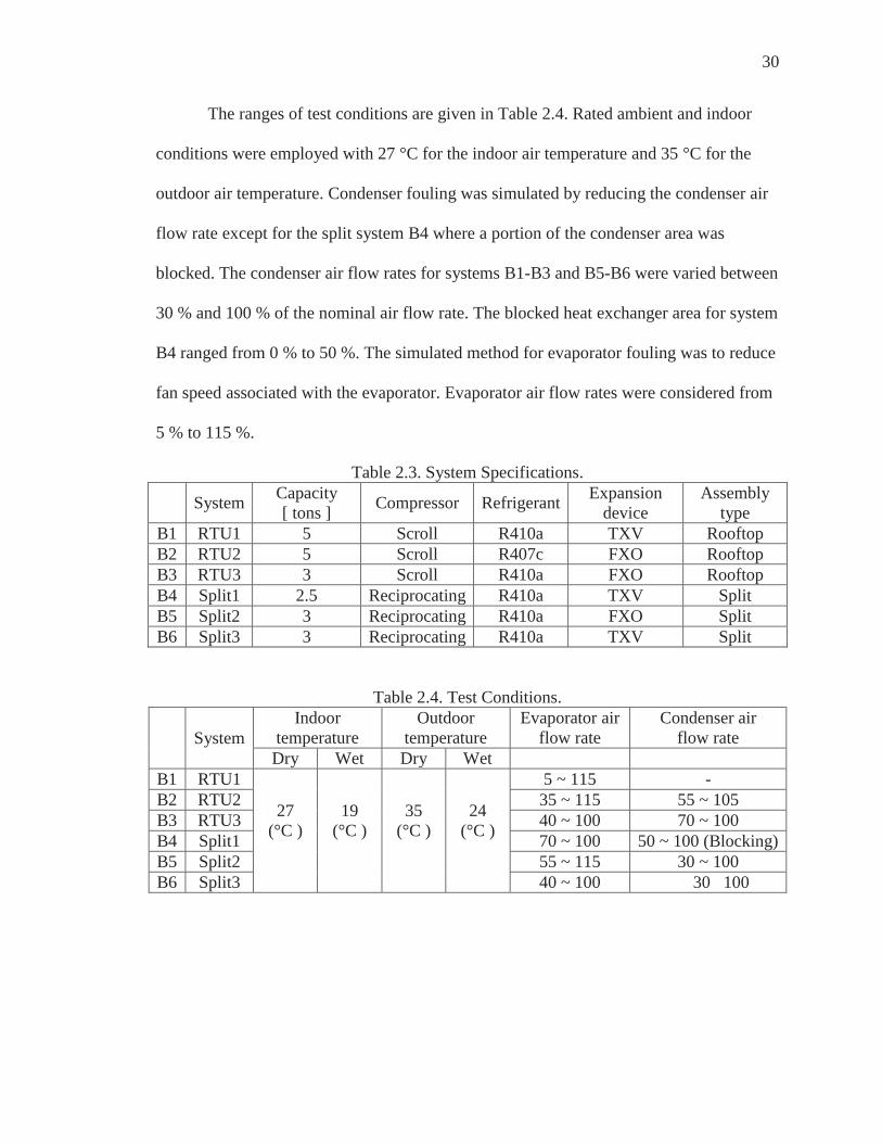
30

The ranges of test conditions are given in Table 2.4. Rated ambient and indoor

conditions were employed with 27 °C for the indoor air temperature and 35 °C for the

outdoor air temperature. Condenser fouling was simulated by reducing the condenser air

flow rate except for the split system B4 where a portion of the condenser area was

blocked. The condenser air flow rates for systems B1-B3 and B5-B6 were varied between

30 % and 100 % of the nominal air flow rate. The blocked heat exchanger area for system

B4 ranged from 0 % to 50 %. The simulated method for evaporator fouling was to reduce

fan speed associated with the evaporator. Evaporator air flow rates were considered from

5 % to 115 %.

Table 2.3. System Specifications. System Capacity

[ tons ] Compressor Refrigerant Expansion device

Assembly type

B1 RTU1 5 Scroll R410a TXV Rooftop B2 RTU2 5 Scroll R407c FXO Rooftop B3 RTU3 3 Scroll R410a FXO Rooftop B4 Split1 2.5 Reciprocating R410a TXV Split B5 Split2 3 Reciprocating R410a FXO Split B6 Split3 3 Reciprocating R410a TXV Split

Table 2.4. Test Conditions.

System Indoor

temperature Outdoor

temperature Evaporator air

flow rate Condenser air

flow rate Dry Wet Dry Wet

B1 RTU1

27 (°C )

19 (°C )

35 (°C )

24 (°C )

5 ~ 115 - B2 RTU2 35 ~ 115 55 ~ 105 B3 RTU3 40 ~ 100 70 ~ 100 B4 Split1 70 ~ 100 50 ~ 100 (Blocking) B5 Split2 55 ~ 115 30 ~ 100 B6 Split3 40 ~ 100 30 100

31

2.3 Impact of Refrigerant Charge and Heat Exchanger Fouling on Performance

2.3.1 Impact of Refrigerant Charge on Performance

2.3.1.1 Impact of Refrigerant Charge for System with a Constant-speed Compressor

Figure 2.1 and 2.2 show the effects of refrigerant charge on cooling capacity and

COP for systems A1-A5. For system A1, the capacity and COP were reduced by 5 %

and 4 %, respectively, with a 25 % decrease of the refrigerant charge amount. The mass

flow rate control provided by an EEV allows the system to compensate for variations in

charge level while maintaining a specified superheat condition at the evaporator outlet.

System A2 and A3 have two cases, with and without an accumulator. A charge

level reduction of 20 % reduced cooling capacity by about 20 % and energy efficiency by

10 % for both cases. The capacity decrease was more significant than for system A1

because this system use an FXO as the expansion device. This caused a reduction in

refrigerant mass flow rate with charge. When the refrigerant charge exceeded 100 %, the

capacity started to decrease for the system without an accumulator because of the

decrease of condensing efficiency that resulted from the surplus refrigerant accumulated

in the condenser.

For system A4, there was a rapid reduction in both cooling capacity and energy

efficiency with decreasing charge below about 70 %. The step change that occurred at 90 %

is due to the fact that only one compressor was operated instead of two compressors

between 90 and 100 % of refrigerant charge level.

For system A5, when the refrigerant was charged less than 70 %, the capacity was

significantly decreased. Although the system uses a TXV the TXV becomes fully open at

32

low charge levels and then the system acts like a system having an FXO as an expansion

device. The COP ratio has the same trend as the capacity. The extreme undercharge of

refrigerant by 60 % reduced cooling capacity by 70 % and energy efficiency by 65 %.

Based on these results, it can be concluded that refrigerant charge levels below

about 80 % of nominal charge can cause significant reductions in both capacity and

energy efficiency. The results also indicate that charge level has a greater impact on

capacity than on efficiency.

Figure 2.1. Capacity ratios for existing test data based on the refrigerant charge.

33

Figure 2.2. COP ratios for existing test data based on the refrigerant charge.

2.3.1.2 Impact of Refrigerant Charge for System with Variable-speed Compressor

This section provides the impact of charge level on cooling capacity, heating

capacity, and efficiency (COP) for a heat pump having a variable-speed compressor.

Figures 2.3 and 2.4 shows cooling capacity and COP normalized by rated values for

system A6. These results are presented as a function of refrigerant charge for different

ambient temperatures and operating frequencies. The nomenclature “MX” and “INT”

refer to maximum (49Hz) and intermediate (27Hz) frequencies. In this particular case, the

results demonstrate that the impact of refrigerant charge on performance was relatively

small if the charge was within 10 % of the rated charge. However, there was a dramatic

reduction in both cooling capacity and energy efficiency with decreasing charge below

about 70 % refrigerant charge.

Overcharging had a somewhat larger effect on COP than undercharging within

this range. When overcharged, the capacity did not show a large degradation, whereas the

34

COP was reduced due to an increase in power consumption. The increased power

consumption was caused by a rise of pressure ratio. There are similar trends for both

frequencies, although the optimal charge for peak capacity and COP moves to lower

values at lower speeds. The impact of refrigerant charge on capacity increased

dramatically with increasing compressor speed and somewhat less dramatically with

decreasing outdoor temperature for this unit. In contrast, the impact of refrigerant charge

on COP was more strongly influenced by outdoor temperature than compressor speed

over the ranges considered.

Figures 2.5 to 2.6 show the performance based on the heating capacity ratio and

COP ratio for system A6 with refrigerant charges between 50 and 150% based on

maximum (105Hz) and intermediate (47Hz) frequencies. The trends are similar to those

for cooling with undercharge resulting in significant capacity and COP reductions at

refrigerant charge levels below 70 %.

The impact of low ambient temperature on capacity and COP is greater than the

charge effect in heating mode. When the ambient temperature decreased to –3.3 °C, the

superheat at the compressor inlet could not be maintained at an appropriate level required

to keep the heat pump running at a stable condition. The degree of subcooling also

became insufficient due to a significant decrease in the condenser pressure. At this low

ambient temperature, the impact of charge on capacity and COP is very small over the

range considered. The impact of refrigerant charge on capacity and COP was more

dependent on compressor speed than outdoor temperature.

Based on the test measurements, refrigerant charge under 70 % can cause

significant reductions in both cooling and heating capacity. On average, a charge

35

decrease of 25 % reduced cooling capacity by 20 % and energy efficiency by 15 %.

Based on the data analyzed in this study, it appears that undercharging a unit based on

charge predictions that are within 10 % of the actual charge would result in less than a 5%

impact on efficiency, whereas overcharging by 10% has a minimal impact on efficiency.

Under or overcharging by 5 % has an insignificant effect on efficiency.

Figure 2.3. Cooling capacity ratios for system A6 based on refrigerant charge.

Figure 2.4. Cooling COP ratios for system A6 based on refrigerant charge.

36

Figure 2.5. Heating capacity ratios for system A6 based on the refrigerant charge.

Figure 2.6. Heating COP ratios for system A6 based on the refrigerant charge.

2.3.2 Impact of Fouling on Performance

Heat exchanger fouling can have two effects on performance. 1) The thermal

resistance of the heat exchanger increases due to deposits collecting on the surfaces. The

conductivity of the deposit is lower than that of the metal of the heat exchanger. 2) The

air flow rate is reduced due to higher pressure drop resulting from the deposits. The

37

reduction of air flow rate can significantly impact the performance of the air conditioner

system. Previous work (Li et.al, 2007) has demonstrated that the effect of reduced air

flow is more significant than that associated with increased thermal resistance.

2.3.2.1 Impact of Evaporator Fouling on Performance

Figures 2.7 and 2.8 show the impact of evaporator fouling on performance

(capacity, and energy efficiency). Fouling was simulated using only reduction of air flow

rate due to pressure drop without the effect of an increase of thermal resistance due to

deposits. On average, the capacity and COP were reduced by 10 % and 6 %, respectively,

with a 40 % reduction of evaporator air flow rate. The results show that the impacts are

relatively small over this range. However, the impact of evaporator fouling on capacity

and COP increases dramatically below about 40% of normal air flow rate. The reduction

of evaporator air flow rate by 50% decreased capacity by 17 %, whereas the energy

efficiency was decreased by 12 %.

The results also show that evaporator fouling has a stronger impact on capacity

than on efficiency. Furthermore, the effect of too high an air flow is relatively small. A

20 % increase of evaporator air flow has a insignificant effect on capacity and efficiency.

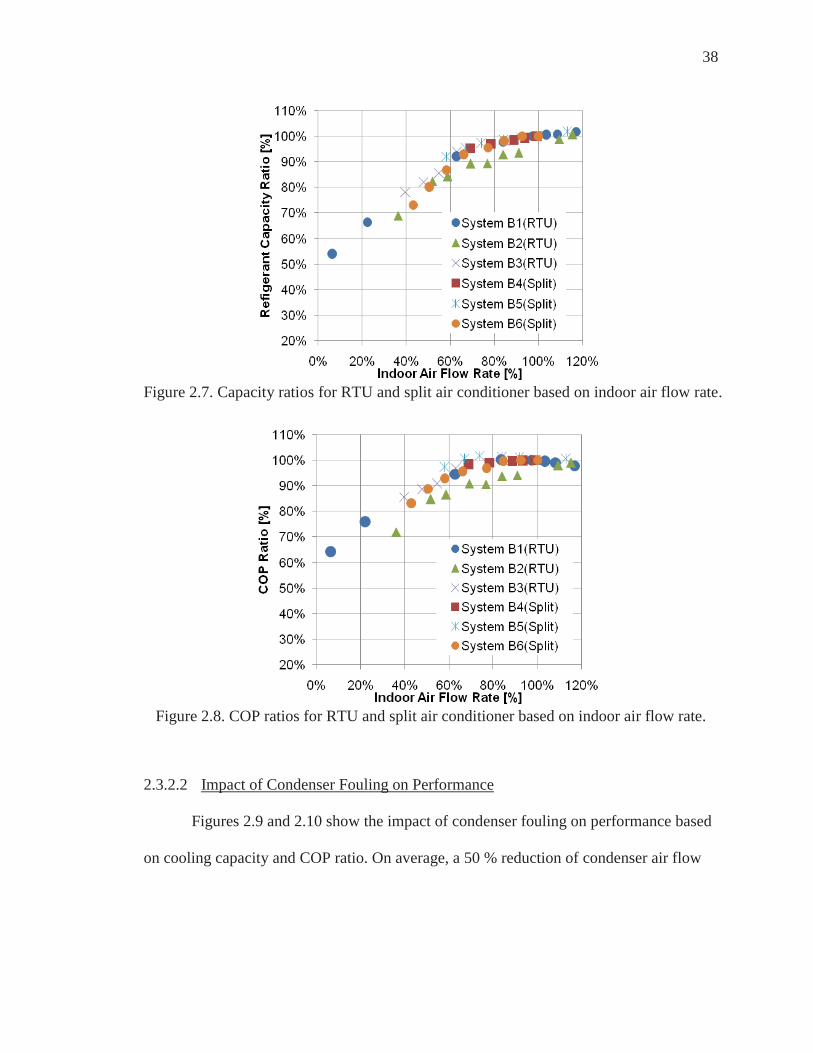
38

Figure 2.7. Capacity ratios for RTU and split air conditioner based on indoor air flow rate.

Figure 2.8. COP ratios for RTU and split air conditioner based on indoor air flow rate.

2.3.2.2 Impact of Condenser Fouling on Performance

Figures 2.9 and 2.10 show the impact of condenser fouling on performance based

on cooling capacity and COP ratio. On average, a 50 % reduction of condenser air flow

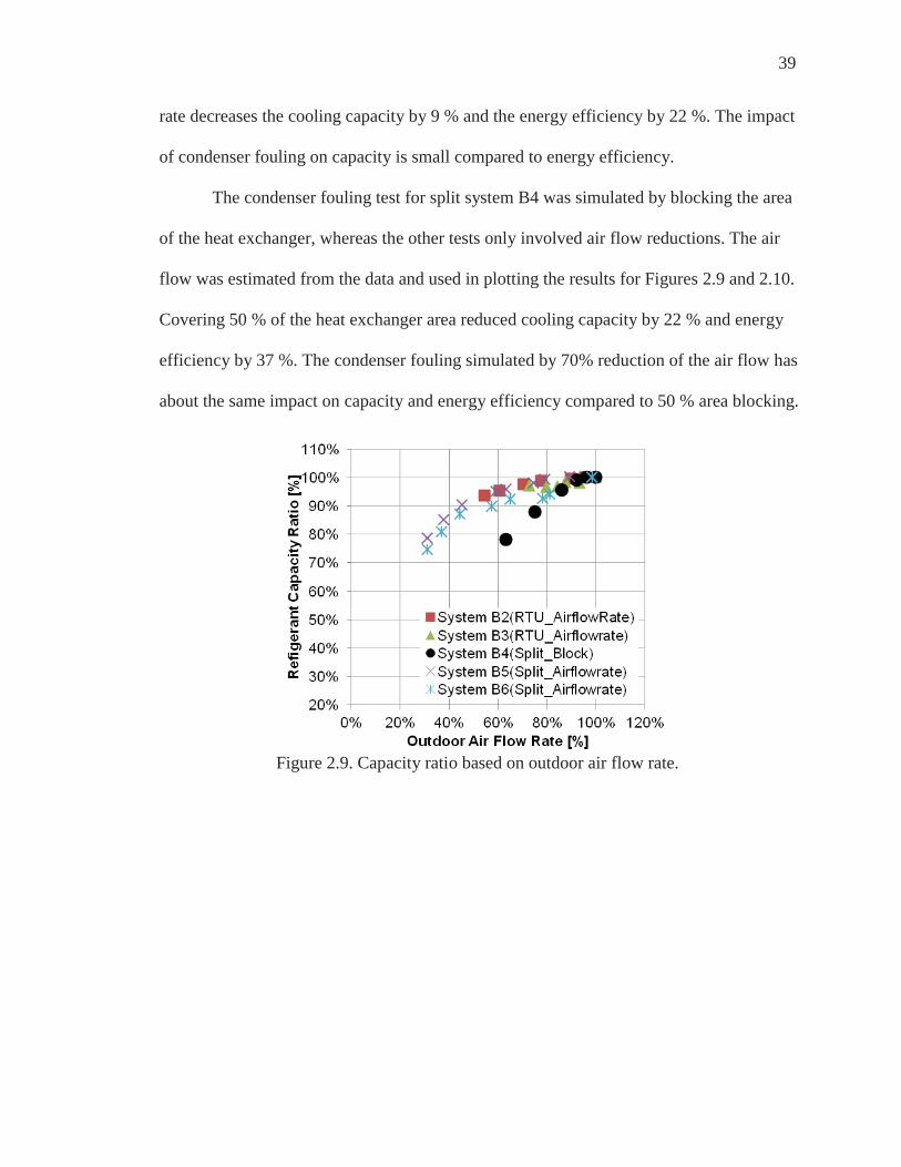
39

rate decreases the cooling capacity by 9 % and the energy efficiency by 22 %. The impact

of condenser fouling on capacity is small compared to energy efficiency.

The condenser fouling test for split system B4 was simulated by blocking the area

of the heat exchanger, whereas the other tests only involved air flow reductions. The air

flow was estimated from the data and used in plotting the results for Figures 2.9 and 2.10.

Covering 50 % of the heat exchanger area reduced cooling capacity by 22 % and energy

efficiency by 37 %. The condenser fouling simulated by 70% reduction of the air flow has

about the same impact on capacity and energy efficiency compared to 50 % area blocking.

Figure 2.9. Capacity ratio based on outdoor air flow rate.

40

Figure 2.10. COP ratio based on outdoor air flow rate.

2.4 Impact of Refrigerant Charge and Heat Exchanger Fouling on Costs

To provide information on the impact of refrigerant charge on operating costs, SEER

and the average cost of electricity were used. The efficiency of air conditioners is rated

using SEER which is defined by the Air Conditioning, Heating, and Refrigeration

Institute in its standard ASHRAE 210 (2010). The higher the SEER rating of a unit, the

more energy efficient it is.

Table 2.5. Bin Weather data for SEER. Number 1 2 3 4 5 6 7 8 9 10 11 12 13 14 15

OD Temp. 24 25 26 27 28 29 30 31 32 33 34 35 36 37 38 Occurring

Hrs. 196 225 225 240 181 122 93 92 35 11 6 4 0 0 0

The average electricity cost for the cost calculation was assumed to be 0.12$/kWh,

based on the U.S. Energy Information Administration’s Electric Power data (February 13,

2009). Table 2.5 shows the bin weather data used in calculating SEER and the total

41

occurring hours from the Table 2.5, 1430 hours, is assumed to be the number of hours of

operation.

The annual cost of electric power consumed for an air conditioner having a specified

rated capacity (Btu/h), number of operating hours per year (h), SEER rating, and cost per

kW·h of electrical usage ($/kW·h) is estimated as

1000)/($.)(..)/(($)...

SEERkwhrateselectrichyearperhourhBtuUnitSizePowerofCostAnnual . (2-7)

2.4.1 Impact of Refrigerant Charge on Energy Costs

Figures 2.11 and 2.12 show calculation results for the SEER ratio and annual cost

ratio of electricity that were determined by using the manufacturers’ and laboratory test

data. Low refrigerant charge can cause decreases in SEER with significantly higher

operating costs.

In the case of system A2 without an accumulator, a 35 % decrease of the

refrigerant charge led to a SEER decrease of 25 % and an annual energy cost increase of

about 30 % (US$ 105 per ton of rated capacity). Using system A2 with an accumulator,

the electricity consumption was increased by 20 % as a result of the SEER value decrease

by 13 % with a loss of about one-third of the nominal charge. For typical electric rates,

this would result in an annual energy cost penalty of about15 % (US$ 52 per ton) for this

unit. In case of the system A4 with tandem compressor, 65 % of normal refrigerant

charge led to a decrease in SEER value of 30 %. The annual operating cost would

increase by about US$ 140 per ton for this system.

42

For system A5 with TXV as the expansion device, a reduction of charge level by

60 % decreased the SEER ratio by 46 %, resulting in an estimated annual cost penalty of

US$ 232 per ton. In the case of system A6 with a variable-speed compressor, a loss of 50 %

of the normal refrigerant charge led to a decrease in SEER value of 45 %, and an annual

energy cost increase of about 70% (US$ 226 per ton of rated capacity).

Figure 2.11. SEER ratios for all test data as a function of refrigerant charge.

Figure 2.12. Annual cost ratios for all test data as a function of refrigerant charge.

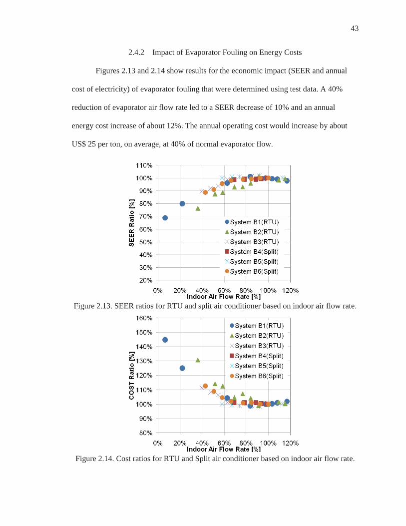
43

2.4.2 Impact of Evaporator Fouling on Energy Costs

Figures 2.13 and 2.14 show results for the economic impact (SEER and annual

cost of electricity) of evaporator fouling that were determined using test data. A 40%

reduction of evaporator air flow rate led to a SEER decrease of 10% and an annual

energy cost increase of about 12%. The annual operating cost would increase by about

US$ 25 per ton, on average, at 40% of normal evaporator flow.

Figure 2.13. SEER ratios for RTU and split air conditioner based on indoor air flow rate.

Figure 2.14. Cost ratios for RTU and Split air conditioner based on indoor air flow rate.

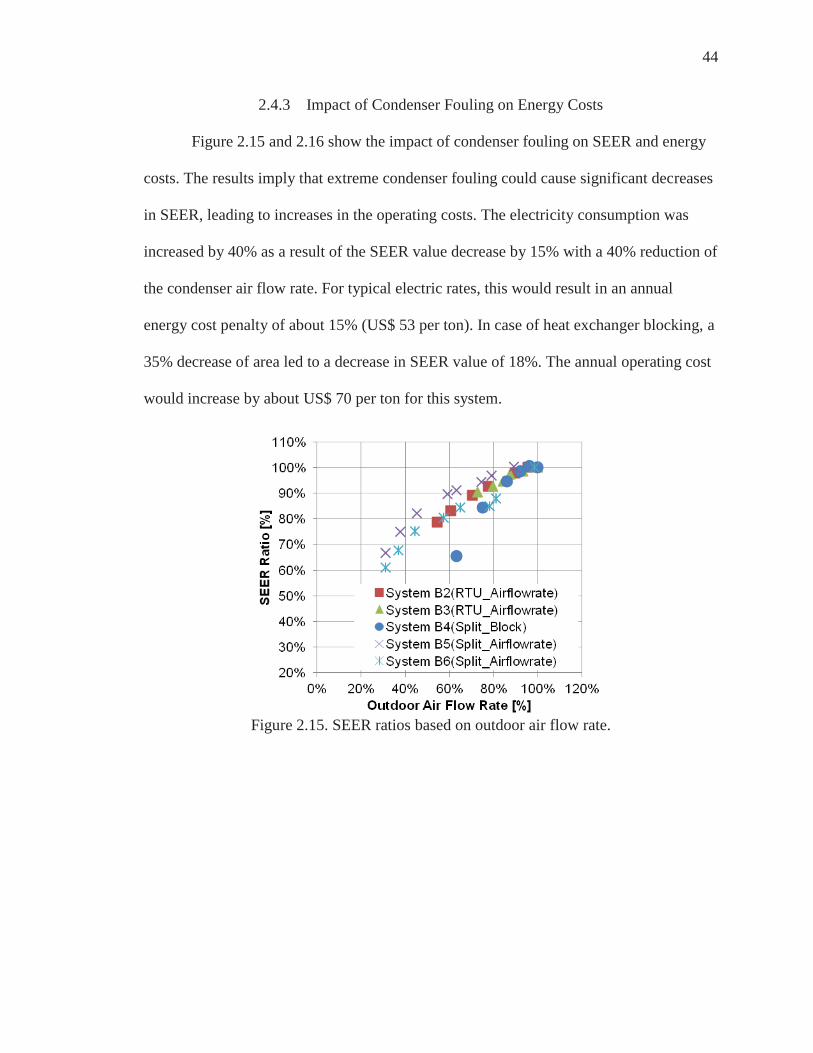
44

2.4.3 Impact of Condenser Fouling on Energy Costs

Figure 2.15 and 2.16 show the impact of condenser fouling on SEER and energy

costs. The results imply that extreme condenser fouling could cause significant decreases

in SEER, leading to increases in the operating costs. The electricity consumption was

increased by 40% as a result of the SEER value decrease by 15% with a 40% reduction of

the condenser air flow rate. For typical electric rates, this would result in an annual

energy cost penalty of about 15% (US$ 53 per ton). In case of heat exchanger blocking, a

35% decrease of area led to a decrease in SEER value of 18%. The annual operating cost

would increase by about US$ 70 per ton for this system.

Figure 2.15. SEER ratios based on outdoor air flow rate.

45

Figure 2.16. Cost ratios based on outdoor air flow rate.

2.5 Summary

Important performance indices for an air conditioner system are cooling capacity

and COP. For systems with an FXO, there is a rapid reduction in both cooling capacity

and energy efficiency with decreasing refrigerant charge level even at charge levels near

normal. For systems with a TXV or EEV, both capacity and COP do not decrease

significantly until the refrigerant charge level reaches around 70 %. When the charge

level is under about 70 %, the TXV (or EEV) becomes fully open and then the system

acts like a system having a FXO.

According to previous research on residential air conditioners, about 55 % of

systems are undercharged by 10 to 30 % due to incorrect measurement of charge level

during installation or service. Based on the results of this study, refrigerant undercharging

in the range of 25 % can lead to an average reduction of 20 % in cooling capacity and 15 %

in energy efficiency. Furthermore, an undercharge of about 25 % would cause an average

46

penalty in SEER of about 16 % and a cost penalty of US$ 60 per year per ton of rated

capacity for typical electricity rates. These penalties could be considered as cost savings

associated with improving refrigerant charge levels and are very significant.

For evaporator fouling, a reduction of air flow rate by 50 % decreased the average

capacity by 14 %, whereas the energy efficiency was decreased by 12 %. The average

SEER value decreased by 10 % and annual cost increased by $24 per ton. For condenser

fouling, a reduction of air flow rate by 50% decreased the average capacity by 9 %,

whereas energy efficiency was decreased by 22 %. The SEER value decreased by 20 %

and annual cost increased by $80 per ton. Evaporator fouling has more influence on

capacity than on efficiency, while condenser fouling has more impact on efficiency.

47

CHAPTER 3. EXTENSION, DEVELOPMENT AND ASSESSMENT OF VIRTUAL SENSORS FOR VARIABLE-SPEED COMPRESSORS

Variable-speed compressors are one of the most energy efficient methods to

regulate capacity for heat pumps and air conditioners because they minimize on/off

cycling (Qureshi et al., 1996; Aprea et al., 2004; Ding, 2007). The fixed-speed

compressor, the dominant type in the air conditioner market in the past, is now gradually

being replaced by the variable-speed compressor for high-efficiency equipment. The use

of variable-speed compressors is common in Asia and has recently started to make in-

roads within the U.S. market for commercial and residential air conditioners. Despite the

expanded application of variable-speed compressors, there are only a few modeling

approaches for compressor performance that have been published (Navarro-Esbrv et al.,

2007; Park et al., 2001; Browne et al., 2002). The primary goal of the work described in

this chapter is to extend a virtual refrigerant charge sensor (VRC) for determining

refrigerant charge and develop virtual refrigerant mass flow (VRMF) and virtual

compressor power (VCP) sensors for equipment having variable-speed compressors and

fans.Extension of Virtual Refrigerant Charge (VRC) Sensor for Variable-Speed

Compressors

The original VRC sensor (Li and Braun: 2007, 2009) uses a correlation in terms

of superheat and subcooling that are determined using low-cost surface mounted

48

temperature sensors. Parameters of the method can be estimated using readily available

manufacturers’ data. Furthermore, the charge estimates are relatively insensitive to the

existence of other system faults. Based on previous research (Kim and Braun: 2012a), the

VRC sensor was found to work well in estimating the refrigerant charge for a range of air

conditioner and heat pumps having fixed-speed compressors. However, none of the tested

equipment included variable-speed compressors.

The typical approach used to verify refrigerant charge for systems having

variable-speed compressors was reviewed. Despite the fact that there are slight

differences between manufacturers, the basic methods are based on using measured

pressure at the service valve determined with a manifold gauge, when the system is

operating at fixed-speed in a test mode set by a remote controller. A technician decides to

add or remove refrigerant based on the difference between a pressure measurement and a

target pressure specified by technical data provided by the manufacturer. These

approaches can only determine whether the charge is high or low, not the level of charge.

In addition, the current charge verification protocols utilize pressure gauges or

transducers installed at the service valve. The installation of these gauges or transducers

can lead to refrigerant leakage. Because of these limitations, the current protocols for

checking refrigerant charge may be doing more harm than good in many situations.

The current research extends the VRC sensor for systems with variable-speed

compressors and fans. To evaluate the accuracy of the VRC sensor, data were first

collected from previous laboratory tests for different systems and over a wide range of

operating conditions. In addition, new laboratory tests were performed to consider

conditions not available within the existing data-set. The systems for the new laboratory

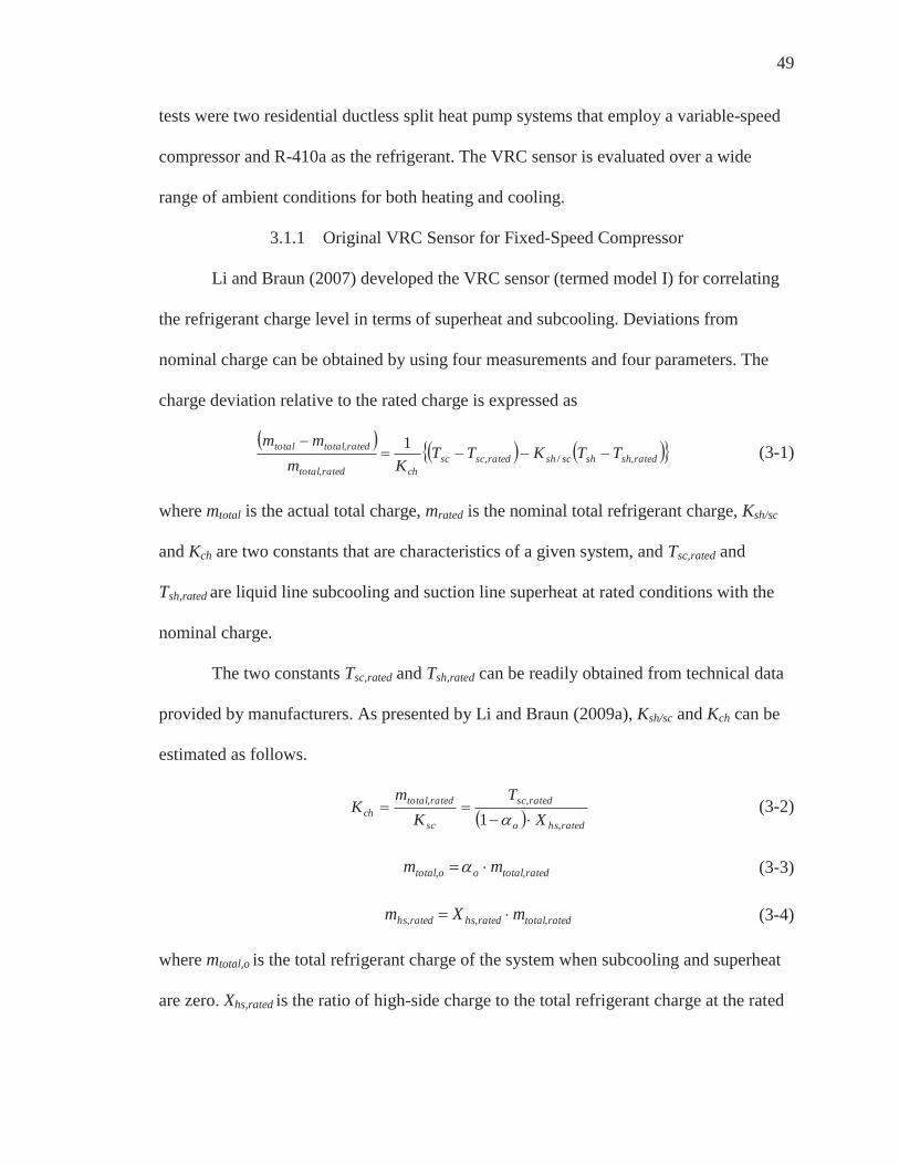
49

tests were two residential ductless split heat pump systems that employ a variable-speed

compressor and R-410a as the refrigerant. The VRC sensor is evaluated over a wide

range of ambient conditions for both heating and cooling.

3.1.1 Original VRC Sensor for Fixed-Speed Compressor

Li and Braun (2007) developed the VRC sensor (termed model I) for correlating

the refrigerant charge level in terms of superheat and subcooling. Deviations from

nominal charge can be obtained by using four measurements and four parameters. The

charge deviation relative to the rated charge is expressed as

ratedshshscshratedscscchratedtotal

ratedtotaltotal TTKTTKm

mm,/,

,

, 1 (3-1)

where mtotal is the actual total charge, mrated is the nominal total refrigerant charge, Ksh/sc

and Kch are two constants that are characteristics of a given system, and Tsc,rated and

Tsh,rated are liquid line subcooling and suction line superheat at rated conditions with the

nominal charge.

The two constants Tsc,rated and Tsh,rated can be readily obtained from technical data

provided by manufacturers. As presented by Li and Braun (2009a), Ksh/sc and Kch can be

estimated as follows.

ratedhso

ratedsc

sc

ratedtotalch X

TK

mK

,

,,

1 (3-2)

ratedtotaloototal mm ,, (3-3)

ratedtotalratedhsratedhs mXm ,,, (3-4)

where mtotal,o is the total refrigerant charge of the system when subcooling and superheat

are zero. Xhs,rated is the ratio of high-side charge to the total refrigerant charge at the rated

50

condition and αo is the ratio of refrigerant charge necessary to have saturated liquid at the

exit of the condenser to the rated refrigerant charge. The parameter Ksc/sh is the slope of a

straight-line plot of (Tsc-Tsc,rated) versus (Tsh-Tsh,rated) for the rated refrigerant charge,

shown in

ratedshsh

ratedscsc

sh

scscsh TT

TTKK

K,

,/ . (3-5)

In this thesis, different approaches were considered for determining Tsc,rated,

Tsh,rated, Ksh/sc and Kch within the refrigerant charge algorithm: 1) use of default values for

all 4 empirical parameters used by the VRC sensor, 2) determination of Kch from

simulations with the other 3 parameters using default values, 3) tuning of Ksh/sc and Kch

using linear regression applied to the measurements.

In order to determine reasonable default parameters, data available from Harms

(2002) was used to estimate a value for Xhs,rated of 0.73 and a value of 0.75 for αo. A

reasonable estimate for Ksh/sc for systems using a thermal expansion valve (TXV) or fixed

orifice (FXO) as the expansion device is 3°C/7.5°C=1/2.5 based on test results. For a

system using an electronic expansion valve (EEV), superheat remains nearly constant

around the rated value regardless of various operating conditions, and the refrigerant

inventory in the evaporator is relatively constant. In this case, the second term in equation

3-1 is approximately zero as

0,/ ratedshshscsh TTK . (3-6)

It is reasonable to choose a default value for Ksh/sc of 0 when the EEV is within the

controllable range. However, at low refrigerant charge the EEV becomes fully open and

then the system acts like a system having a FXO. In this case, a more appropriate value

51

for Ksh/sc can be determined through regression using data over a range of refrigerant

charge levels.

To improve charge predictions, a simulation method for estimating Kch was

developed for extremely overcharged and undercharged refrigerant levels (Kim and

Braun, 2012a). The simulation method determines this empirical parameter using a

physical description of the heat exchangers and piping along with measurements at rated

conditions and the nominal charge level. Kch should depend on three elements of each

system: the liquid line length, the rated subcooling, and the rated charge. Different split

and packaged systems can have very different liquid line lengths. The rated subcooling

and the rated charge also vary, depending on each unit. Based on those findings, Kch can

be calculated from the refrigerant mass distribution in the system. Table 3.1 shows

comparisons of parameters determined from this calculation approach with parameters

determined directly from the measurements of Harms (2002) for three different air

conditioners. For these calculations, a void fraction correlation based on the slip ratio

equation from Zivi (1964) was found to give the best results for the data. Overall, the

simulation approach provides reasonable estimates of αo and Xhs,rated for different split

and packaged systems with different liquid line lengths.

Table 3.1. Comparison between parameters based on measurements and calculation.

System from measurements by Harms from simulation approach Kch αo Xhs,rated Kch αo Xhs,rated

2.5 ton split 56.76 0.73 0.73 60.81 0.72 0.71 5 ton packaged 23.97 0.7 0.78 32.26 0.77 0.76

7.5 ton split 59.29 0.82 0.68 57.81 0.78 0.56

Alternatively, Ksc/sh and Kch for the VRC sensor can be tuned to improve accuracy

if data are available over a range of refrigerant charge levels and operating conditions. It

52

is necessary to have variations in charge level to adequately determine parameters, but

the data could also include variations in outdoor air flow rate, indoor air flow rate,

ambient temperature, and indoor dry bulb temperature. The parameter tuning method

minimizes the errors between predicted and known refrigerant charge using linear

regression. Given a set of measurements, parameters are estimated with

MTTTK TT 1 (3-7)

where K is a parameter vector given as shown in

T

ch

scsh

ch KK

KK /1 . (3-8)

The vector M is a set of m deviations from nominal refrigerant charge determined

from measurements and given as shown in

TVRCVRCVRC mmmM 4,2,1, . (3-9)

The matrix T contains a set of m inputs determined from measurements defined

as

mshmsc

shsc

shsc

TT

TTTT

T

,,

2,2,

1,1,

. (3-10)

The individual elements in equations 3-9 and 3-10 are determined from

measurements and defined as

ratedtotal

ratedtotaltotalVRC m

mmm

,

, , ratedscscsc TTT , , ratedshshsh TTT , (3-11)

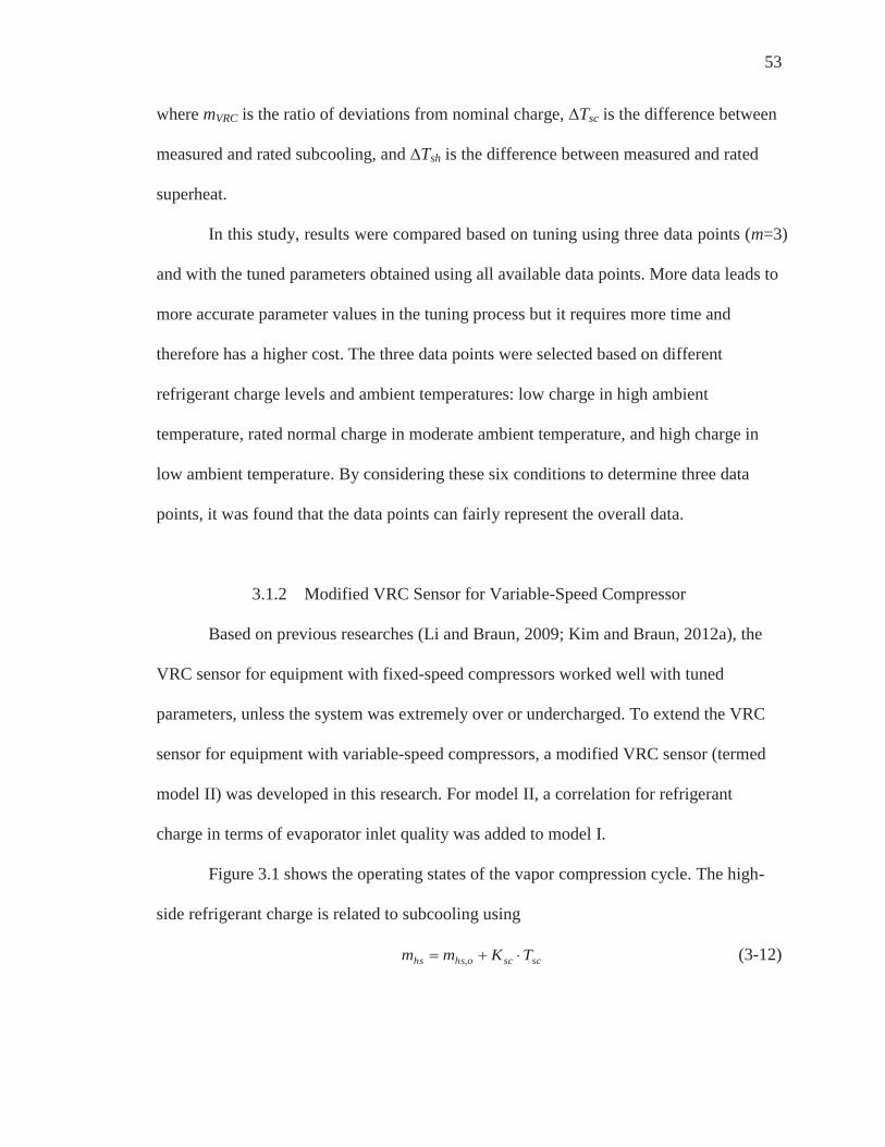
53

where mVRC is the ratio of deviations from nominal charge, ∆Tsc is the difference between

measured and rated subcooling, and ∆Tsh is the difference between measured and rated

superheat.

In this study, results were compared based on tuning using three data points (m=3)

and with the tuned parameters obtained using all available data points. More data leads to

more accurate parameter values in the tuning process but it requires more time and

therefore has a higher cost. The three data points were selected based on different

refrigerant charge levels and ambient temperatures: low charge in high ambient

temperature, rated normal charge in moderate ambient temperature, and high charge in

low ambient temperature. By considering these six conditions to determine three data

points, it was found that the data points can fairly represent the overall data.

3.1.2 Modified VRC Sensor for Variable-Speed Compressor

Based on previous researches (Li and Braun, 2009; Kim and Braun, 2012a), the

VRC sensor for equipment with fixed-speed compressors worked well with tuned

parameters, unless the system was extremely over or undercharged. To extend the VRC

sensor for equipment with variable-speed compressors, a modified VRC sensor (termed

model II) was developed in this research. For model II, a correlation for refrigerant

charge in terms of evaporator inlet quality was added to model I.

Figure 3.1 shows the operating states of the vapor compression cycle. The high-

side refrigerant charge is related to subcooling using

scscohshs TKmm ,

(3-12)

54

where mhs is the charge in the high-pressure side of the system, mhs,0 is the high-side

refrigerant mass for the case of zero subcooling and Ksc is a constant that depends on the

condenser geometry. mhs,o is assumed to be a constant, independent of operating

conditions and total charge.

The low-side charge is related to superheat and inlet quality for the evaporator

based on

inevaposcxshsholsls xxKTKmm ,,,

(3-13)

where mls,o is the low-side refrigerant mass for the case of zero superheat and zero

subcooling, xevap,in is the evaporator inlet quality, Kx is a constant characteristic of a given

system, and Ksh is a constant that depends on the evaporator geometry. mls,o is assumed to

be a constant, independent of operating conditions and total charge. The subscript ‘sc,o’

denotes that the case of zero subcooling is employed.

Equations 3-12 and 3-13 can be applied to all operating conditions including the

rated condition, shown as

ratedscscohsratedhs TKmm ,,,

(3-14)

ratedinevaposcxratedshsholsratedls xxKTKmm ,,,,,,

(3-15)

where the subscript ‘rated’ denotes that the rating operating conditions are employed.

Tsc,rated and Tsh,rated are liquid line subcooling and suction line superheat, respectively, at

rated conditions with the nominal charge, respectively.

Equations 3-12 to 3-15 can be combined to give expressions for changes from

rated conditions in subcooling, superheat, and inlet quality of the evaporator in terms of

charge variation by eliminating mhs,o and mls,o shown as follows.

55

)()( ,, ratedhshsratedscscsc mmTTK .

(3-16)

)()()( ,,,,, ratedlslsratedinevapinevapxratedshshsh mmxxKTTK . (3-17)

Equations 3-16 and 3-17 are combined and the result is manipulated to give a

single expression that relates subcooling, inlet quality of the evaporator, and superheat to

the total refrigerant charge.

)()()(

)()(

,,,,,

,,

ratedinevapinevapxratedshshshratedscscsc

ratedlslsratedhshs

xxKTTKTTK

mmmm

. (3-18)

)()()()( ,,,,,, ratedinevapinevapxratedshshshratedscscscratedtotaltotal xxKTTKTTKmm . (3-19)

Equation 3-19 is then manipulated to give the deviation from rated charge relative

to rated charge as a function of three inputs determined from measurements (Tsc, Tsh,

xevap,in) and seven constants (Ksc, Ksh/sc, Kx/sc, mtotal,rated, Tsc,rated, Tsh,rated, xevap,in,rated).

)()()()(

,,,,,,,

,ratedinevapinevap

sc

xratedshsh

sc

shratedscsc

ratedtotal

sc

ratedtotal

ratedtotaltotal xxKKTT

KKTT

mK

mmm (3-20)

)()()(1)(,,,/,/,

,

,ratedinevapinevapxscratedshshshscratedscsc

chratedtotal

ratedtotaltotal xxKTTKTTKm

mm (3-21)

where Ksc/sh, Ksc/x and Kch are three empirical constants that must be estimated for a given

system and the other four parameters are directly determined from measurements at the

rated condition and nominal charge level. The quality entering the evaporator can be

readily estimated using measurements at the condenser exit and assuming an isenthalpic

expansion process.

In Equation 3-21, it is necessary to know Ksc/x . Default estimates of this empirical

parameter can be determined from data at the rated condition. The total refrigerant of a

56

normally charged system under the rated condition can be calculated with the case of zero

superheat and zero subcooling.

)( ,,,,, ratedinevaposcxshshscscototalratedtotal xxKTKTKmm . (3-22)

Plugging equation 3-3 into equation 3-22, equation 3-23 can be obtained.

)()()( ,,,/,/,,, ratedinevaposcxscratedshshscratedscscratedtotaloratedtotal xxKTKTKmm . (3-23)

Substituting equation 3-4 into equation 3-23 results in equation 3-24.

)(1

,,,/,/,,

ratedinevaposcxscratedshshscratedscsc

oratedtotal xxKTKTK

m

. (3-24)

Figure 3.1. Operating states of the vapor compression cycle.

The equation 3-2 was used as

)(1

,,,/,/,,

,,ratedinevaposcxscratedshshscratedsc

ratedhs

ratedsc

sc

oratedtotal xxKTKTXT

Km . (3-25)

57

An expression for estimating Ksc/x is determined as

)( ,,,/,/,

,,,ratedinevaposcxscratedshshsc

ratedhs

ratedscratedhsratedsc xxKTKX

TXT (3-26)

)()(1

,,,

,/

,,,

,

,

,/

ratedinevaposc

ratedshshsc

ratedinevaposc

ratedsc

ratedhs

ratedhsxsc xx

TK

xxT

XX

K . (3-27)

Under low compressor speed conditions with low ambient temperature, the

laboratory test results for this study had zero subcooling and superheat. In these cases,

neither the model I nor model II approach, which use subcooling and superheat

measurement as input parameters, can accurately predict the charge level. Therefore, a

model III approach was developed to provide improved performance in these situations.

Model III is a modification of the model II equation that includes a correlation for

refrigerant charge in terms of the discharge superheat of the compressor.

)()()()(1

)(

,/,,,/,/,

,

,

rateddshdshdshscratedinevapinevapxscratedshshshscratedscscch

ratedtotal

ratedtotaltotal

TTKxxKTTKTTK

mmm

(3-28)

where Ksc/dsh is a constant characteristic of a given system, and Tdsh,rated is the discharge

superheat of the compressor at rated conditions with the nominal charge.

3.1.3 Performance of VRC sensor for Cooling Equipment with Variable-Speed

Compressor

3.1.3.1 System descriptions and test conditions

To evaluate the VRC sensor, data for air conditioners and chillers with variable-

speed compressors were collected where the effects of refrigerant charge on performance

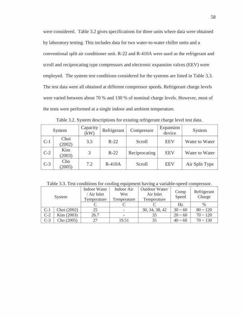
58

were considered. Table 3.2 gives specifications for three units where data were obtained

by laboratory testing. This includes data for two water-to-water chiller units and a

conventional split air conditioner unit. R-22 and R-410A were used as the refrigerant and

scroll and reciprocating type compressors and electronic expansion valves (EEV) were

employed. The system test conditions considered for the systems are listed in Table 3.3.

The test data were all obtained at different compressor speeds. Refrigerant charge levels

were varied between about 70 % and 130 % of nominal charge levels. However, most of

the tests were performed at a single indoor and ambient temperature.

Table 3.2. System descriptions for existing refrigerant charge level test data.

Table 3.3. Test conditions for cooling equipment having a variable-speed compressor.

System Indoor Water

/ Air Inlet Temperature

Indoor Air Wet

Temperature

Outdoor Water/ Air Inlet

Temperature Comp Speed

Refrigerant Charge

C C C Hz % C-1 Choi (2002) 25 - 30, 34, 38, 42 30 ~ 60 80 ~ 120 C-2 Kim (2003) 26.7 - 35 20 ~ 60 70 ~ 120 C-3 Cho (2005) 27 19.51 35 40 ~ 60 70 ~ 130

System Capacity (kW) Refrigerant Compressor Expansion

device System

C-1 Choi (2002) 3.5 R-22 Scroll EEV Water to Water

C-2 Kim (2003) 3 R-22 Reciprocating EEV Water to Water

C-3 Cho (2005) 7.2 R-410A Scroll EEV Air Split Type

59

3.1.3.2 Evaluation of VRC Sensor for a Air Conditioner Equipment with Variable-

Speed Compressors

The VRC sensor was evaluated in terms of RMS deviation between predicted and

actual charge levels relative to nominal charges for the cooling systems having variable-

speed compressors. The test data did not provide information necessary to estimate

parameters using the simulation approach. Therefore, models I and II were only evaluated

based on the use of default and tuned parameters. Figures 3.2 to 3.5 show the

performance of the VRC sensor model I and II based on the default and tuned parameters.

Figures 3.2 shows the performance of the VRC sensor based on model I with

default parameters. Overall, the RMS errors of the VRC sensor algorithm for model I

were 8% based on default parameters. In many cases, the accuracy of the refrigerant

charge predictions is good when using default parameters. However, the use of the

default parameters led to some significant errors greater than 10% in refrigerant charge

estimates at both low and high charge levels with low compressor frequencies.

When the VRC sensor model II with default parameters was applied, there was an

improvement compared to using model I with RMS errors of 6 % shown in Figure 3.3.

Model II with default parameters can also lead to significant improvements in cases

where model I does not work well, such as at extremely low outdoor temperatures and

high charge levels. However, there were still some points with significant refrigerant

charge estimate errors at high charge levels with low compressor frequencies.

To increase the accuracy of the VRC sensor, the parameters were tuned for each

specific system based on measurements obtained at different refrigerant charge levels.

60

When tuned parameters were applied to models I and II, the VRC sensor showed better

performance than when the default parameters were applied, as shown in Figures 3.4 and

3.5.

The RMS errors were reduced to 4 % for model I and 3 % for model II. The

results verified that tuned parameters significantly improve the accuracy of the VRC

sensor. It can be seen that when the system is not over charged, model I with tuned

parameters has good performance under various compressor speeds. However, when the

system is extremely over charged, model I may have significant errors. Compared to

model I, model II led to some improvements in cases where model I did not work well,

such as low compressor speed and high charge level. Overall, the VRC sensor using

model II with tuned parameters can provide very accurate estimates of refrigerant charge

level for cooling systems having variable-speed compressors.

Figure 3.2. Performance of VRC sensor model I based on default parameters for cooling

equipment with variable-speed compressor.

61

Figure 3.3. Performance of VRC sensor model II based on default parameters for cooling




62



3.1.4 Performance of the VRC sensor for Air conditioner Equipment with Fixed-Speed

Compressors

3.1.4.1 System Descriptions and Test Conditions for Air Conditioner Equipment with

Fixed-Speed Compressors

In order to evaluate the VRC sensor model II with the simulation method for

parameter estimation, additional existing laboratory data for fixed-speed compressor

systems were used from Kim and Braun (2012a). For two systems, data were obtained

from the manufacturer. For another two systems, laboratory test data were obtained. The

specifications for the four systems are shown in Table 3.4. Table 3.5 shows the range of

refrigerant charge and other conditions considered for each unit.

For manufacturers’ data C-4 (tandem compressor and an EEV as expansion

device) and system C-5 (rotary compressor and a FXO as expansion device ) with and

63

without an accumulator, the refrigerant charge levels varied between about 60% and 100%

of nominal with an indoor temperature of 27 C and an ambient temperature of 35 C for

cooling conditions. R-22 was used as the refrigerant and only nominal airflow rates were

considered for the evaporator and condenser. Evaporator superheat and condenser

subcooling were determined using pressure and refrigerant temperature measurements.

Although there was not sufficient data available to confirm the accuracy of the

measurements, the data were regarded as accurate considering the ARI standard based

procedures that the commercial company had followed.

Systems C-6 and C-7 (scroll compressor and TXV as expansion device) were

tested at the Herrick Laboratories with the refrigerant charge varied from about 40 % to

130 % of normal charge. The tests were performed under different outdoor temperatures

for cooling mode. Measurements of air-side and refrigerant-side capacities were

compared in order to evaluate the validity of the data. In general, the differences were

less than 5 percent. In addition, uncertainties in superheat and subcooling were evaluated

and were about ±0.6 C for both systems.

Table 3.4. System descriptions for cooling equipment with fixed-speed compressors.

System Capacity (kW) Refrigerant Compressor Accumulator Expansion

device Type

C-4 14.5 R-22 Tandem Yes EEV

Air Split

C-5 15.2 R-22 Rotary Yes FXO No C-6 10.5 R-22 Scroll Yes TXV C-7 10.5 R-410A Scroll Yes

64

Table 3.5. Test conditions for cooling equipment having a fixed-speed compressor.

System Indoor Temp. Outdoor

Temp. Indoor Air Flow rate Refrigerant Charge Level Dry Wet Dry (F) (F) (F) [%] (%)

C-4

80 67 95 100

80 ~ 100

C-5 60 ~ 110 65 ~ 100

C-6 67/ 95 / 105 50 / 100 70 ~ 130 C-7 43 / 95 / 115 100 40 ~ 130

3.1.4.2 Evaluation of VRC Sensor for A/C Equipment with Fixed-Speed Compressors

Performance of the VRC sensor based on model II was compared with the model

I, for systems with fixed-speed compressors. Figures 3.6 and 3.7 show the performance

of the VRC sensor model I and model II based on the simulation parameters. Results of

model I and II showed relatively large errors in predicted refrigerant charges at low

charge level based on simulation parameters.

Figure 3.6 presents performance of the VRC sensor model I based on simulation

parameters. The overall RMS error of VRC sensor model I was about 12 %. As the

refrigerant charge level decreased, there were bigger differences between predicted and

actual charge amounts. The errors were also large at low ambient temperature. For

example, the VRC sensor predicted 60 % of nominal charge when the system was

charged at 40 % of nominal charge. Figure 3.7 shows results of VRC sensor model II

based on the simulation parameters. The overall RMS error of model II was about 11 %.

The use of model II did not lead to improvements in many cases where model I did not

work well.

When model I and II were applied using tuned parameters, the VRC sensor

showed better performance than when the simulation parameters were applied, as shown

65

in Figures 3.8 and 3.9. The RMS errors were reduced to 7% for model I and 6% for

model II. The VRC model I and II using tuned parameters gave similar and accurate

charge predictions for systems with fixed-speed compressors.

Figure 3.6. Performance of VRC sensor model I based on simulation parameters for

cooling equipment with fixed-speed compressors.


cooling equipment with fixed-speed compressors.

66

Figure 3.8 shows the performance of the VRC sensor model I based on tuned

parameters. There was a significant overall improvement for refrigerant charge less than

100%. For extreme test conditions such as low outdoor temperatures, the VRC sensor

model I with tuned parameters needed to be improved to predict all charge amounts

within 10%. Figure 3.9 shows the performance of VRC sensor model II based on tuned

parameters. The performance of model II is very good over a wide range of refrigerant

charge levels and operating conditions. In particular, model II based on tuned parameters

showed better performance than when model I with tuned parameters when applied at

low charge levels.


equipment with fixed-speed compressors.

67


equipment with fixed-speed compressors.

Overall, models I and II with tuned parameters showed good performance in

terms of predicting charge levels for systems with a constant-speed compressor.

However, when test conditions were at low outdoor temperature with low refrigerant

charge, VRC model II can lead to improvements in cases where the model I parameters

do not work well.

68

3.1.5 Performance of the VRC Sensor for Heat Pump Systems with Variable-speed

Compressors

3.1.5.1 System descriptions and test conditions for heat pump systems with variable-

speed compressors

The primary limitations of the previously available data for systems with variable-

speed compressors are that the test conditions were limited to 1) cooling mode only, 2) 70%

as the lowest refrigerant charge level, 3) one ambient temperature condition, and 4)

systems that do not incorporate multi-speed fans. To better assess the accuracy and

broaden the application of the VRC sensor, new test plans were established to consider

the following key issues: 1) heating mode operation for heat pumps, 2) various ambient

temperature conditions, 4) lower levels of refrigerant charge, and 5) systems with multi

speed fans. Two heat pump systems having a variable-speed compressor and multi-speed

fans were selected for testing and installed within the psychrometric chambers at the

Herrick Laboratories. Table 3.6 provides an overview of the two systems that were tested.

R-410A was used as the refrigerant for both systems and a rotary type compressor and

EEV were employed.

The ranges of test conditions in cooling and heating mode are given in Table 3.7.

The test matrix was designed to consider both cooling and heating mode operation with

low levels of refrigerant charge and low ambient temperatures. Data for relatively low

ambient temperatures in cooling were necessary to test the validity of the algorithm

during off-season conditions, when regular maintenance procedures are often performed.

69

Refrigerant charge levels were varied between 50% and 130% of nominal charge levels

with outdoor temperatures between about 67 F and 110 F for cooling mode and 17 F

and 47 F for heating mode. The effects of reduced indoor air flow were also considered

for system C-8, with airflow rates from 260 to 430 [CFM] for heating and cooling mode.

The variable compressor speeds were considered from 18 to 65 Hz in cooling mode and

from 18 to 130 Hz in heating mode.

Table 3.6. System description for heat pump systems having a variable-speed compressor.

System Size (kW)

Refrigerant Type Compressor Expansion

Device Accumulator Assembling Type

C-8 3.5 R-410A Rotary EEV Yes Split C-9 3.5 R-410A Rotary EEV Yes Split

Table 3.7. Test conditions for heat pump systems having a variable-speed compressor.

System Mode

Indoor Temp.

Outdoor Temp. Compressor

Speed

Indoor Fan

Speed

Refrigerant Charge Level Dry Wet Dry

(F) (F) (F) [Hz] [CFM] (%)

C-8 Cooling 80 67 110 / 95 / 67 21 ~ 65 430 /260 50 ~ 130 Heating 70 - 47 / 37 / 17 21 ~ 130 430 /260 50 ~ 130

C-9 Cooling 80 67 105 / 95 / 67 18 ~ 49 410 50 ~ 130 Heating 70 - 47 / 27 / 17 18 ~105 410 50 ~ 150

3.1.5.2 Sensor Locations for the VRC Sensor Applied to Heat Pump Systems

The VRC sensor uses measured temperatures to calculate subcooling and

superheat. Surface-mounted temperature sensors are utilized within the VRC sensor to

determine subcooling (condenser saturated temperature (Tc,sat) - liquid line temperature)

and superheat (suction line temperature - evaporator saturation temperature (Te,sat) ). In

order to determine the best location to measure the temperatures in both heating and

cooling modes, thermocouples were installed at several locations on each indoor and

70

outdoor heat exchanger of a heat pump system with a variable-speed compressor. The

wire thermocouples were soldered to the tube bends of the indoor and outdoor heat

exchangers and insulated to measure the saturation temperatures presented in Figures

3.11 and 3.12. Heat pump tests were performed at different compressor speeds and

ambient temperature conditions. When appropriate sensor locations are chosen, then the

surface mounted temperatures provide estimates of refrigerant saturation temperatures.

The best locations for sensors to measure Tc,sat and Te,sat were identified through

comparisons of saturation temperatures determined from pressure measurements.

Figures 3.12 to 3.15 show comparisons of saturation temperatures based on

pressure and temperature measurements for cooling and heating mode. The evaporator

saturation temperature can be estimated using a surface mounted thermocouple located

on the inlet tube to the evaporator. However, the saturated condenser temperature

requires that the sensor be located on a return somewhere in the middle of the coil where

a two-phase condition exists under a wide variety of conditions. For only cooling mode,

four measurements are necessary to estimate subcooling and superheat. The research

found that a total of six sensors, instead of eight sensors were necessary to determine

subcooling and superheat for both heating and cooling mode. Evaporating and liquid line

temperature sensors in cooling mode are swapped as liquid line and evaporating

temperature sensors in heating mode. Overall, for the system C-9, RMS differences

between saturation temperatures determined using surface mounted sensors and values

determined from pressure measurements were 1.85 C on average for both cooling and

heating mode. A description of the locations for the six sensors is provided in Table 3.8.

71

Figure 3.10. Sensor locations of indoor unit heat exchanger for cooling and heating mode.

Figure 3.11. Sensor locations of outdoor unit heat exchanger for cooling and heating

mode.

72

Figure 3.12. Comparison between evaporator saturation temperature based on pressure measurements and based on temperature measurements for different compressor speeds

in cooling mode (OD Temp: 95F).

Figure 3.13. Comparison between condenser saturation temperature based on pressure measurements and based on temperature measurements for different compressor speeds

in cooling mode (OD Temp: 95F).

73

Figure 3.14. Comparison between evaporator saturation temperature based on pressure measurements and based on temperature measurements for different compressor speeds

in heating mode (OD Temp: 47F).

Figure 3.15. Comparison between condenser saturation temperature based on pressure measurements and based on temperature measurements for different compressor speeds

in heating mode (OD Temp: 47F).

74

Table 3.8. Sensor locations for heat pump units in cooling mode and heating mode. Sensor Heating mode sensor location Cooling mode sensor location

Condenser Saturation

Temperature Sensor

Indoor Unit Sensor 12 (Condenser Intermediate Temp)

Outdoor Unit Sensor 10 (Condenser Intermediate Temp)

Liquid Line Temperature Sensor

Indoor Unit Sensor 1 (Condenser Outlet Temp)

Outdoor Unit Sensor 9 (Condenser Outlet Temp)

Evaporator Saturation

Temperature Sensor

Outdoor Unit Sensor 9 (Evaporator Inlet Temp)

Indoor Unit Sensor 1 (Evaporator Inlet Temp)

Suction Line Temperature Sensor

Outdoor Unit Sensor 7 (Suction Line Temperature)

Indoor Unit Sensor 7 (Suction Line Temperature)

3.1.5.3 Evaluation of VRC sensor for Heat Pump Systems with Variable-Speed

Compressor

Figures 3.16 to 3.19 show the accuracy of the VRC sensor for the heat pump

systems in cooling and heating modes. The performance was evaluated in terms of RMS

deviation from the actual charge levels presented on a percentage basis for models II and

III.

Figure 3.16 shows the performance of the VRC sensor based on model II and

default parameters in cooling and heating mode. Based on the RMS errors of 16 % for

cooling mode and 22 % for heating mode, the VRC sensor did not perform well in

predicting the charge level. As the fault level of refrigerant charge increased or decreased,

there was a bigger difference between estimated and actual charge amounts. For example,

model II with default parameters predicts 20 % undercharge when the system is charged

at 50% of the nominal charge. When the ambient temperature and compressor speed were

low, the refrigerant charge error increased compared to other test conditions.

75

Figure 3.17 shows results based on the use of parameters that were determined

using the simulation approach. Model II based on simulation parameters showed RMS

errors of 15 % for cooling mode and 20 % for heating mode. The use of simulation

parameters led to significant errors in refrigerant charge estimates at low and high charge

level. The errors were relatively large at low compressor speed conditions when the

system was overcharge conditions. Overall, model II with simulation parameters did not

improve the performance of the VRC sensor compared to the default parameters for the

heat pump system.

Figure 3.18 shows performance based on tuned parameters. The RMS errors were

reduced to 13 % for cooling mode and 12 % for heating mode. When tuned parameters

were applied in heating mode, there was a significant improvement compared to using the

default and simulation parameters. Although the RMS error is reduced, the errors at high

charge levels are greater with more variability in the predictions. The errors are large at

high charge levels because the superheat exiting the compressor was nearly zero for

various operating conditions. The VRC sensor model II with tuned parameters

underestimates charge when the system is highly overcharged with errors up to 30% at a

charge level of 130 %. In cooling mode, the large deviations still remained at conditions

having zero subcooling.

Figure 3.19 shows the performance of model III based on tuned parameters. In

this case, the RMS errors were reduced to 10% for cooling and 7 % for heating mode. In

heating mode, model III can lead to significant improvements in cases where models I

and II do not work well, such as at overcharge conditions with extremely low outdoor

temperatures and low compressor speed. Overall, VRC model III is better than the other

76

two models for characterizing refrigerant charge levels for heat pumps with variable-

speed compressors. However, there were still some significant errors at low ambient

temperatures and low speeds when subcooling was zero.

Figure 3.16. Performance of VRC sensor model II based on default parameters for heat

pumps.


heat pumps.

77

Figure 3.18. Performance of VRC sensor model II based on tuned parameters for heat

pumps.

Figure 3.19. Performance of VRC sensor model III based on tuned parameters for heat

pumps.

3.1.6 Comparison with Manufacturer’s Charging Method

The charging method specified by the manufacturer for system C-9 was applied

and compared with the VRC sensor based on model III for cooling mode. The approach

78

used to verify refrigerant charge in the field for this system involves the use of pressure at

the service valve. Suction pressure for cooling mode and discharge pressure for heating

mode are used to indicate the charge level with the compressor operating at a fixed-speed

in a test mode. The technicians can evaluate whether to add or remove refrigerant based

on a difference between the pressure measurement and a target pressure.

Figure 3.20 shows measurements associated with applying the manufacturer’s

refrigerant charge protocol for system C-9 in cooling mode at three different ambient

temperatures. The three horizontal lines correspond to the target suction pressures at the

three temperatures. Although the suction pressure increases with charge level, it doesn’t

achieve the target even at 130% of normal charge. The deviation between the measured

and target pressure is greatest at the lowest outdoor temperature. It appears that current

approaches would have difficulty in identifying the proper charge amount during off-

season maintenance.

Figure 3.20. Refrigerant charge method based on manufacturer’s method for cooling mode (System C-9).

79

Figure 3.21 shows performance of model III based on tuned parameters using the

data at maximum compressor speed in cooling mode. The VRC sensor provides accurate

refrigerant charge estimates in cooling mode regardless of the ambient temperature.

Figure 3.21. Performance of VRC sensor model III based on tuned parameters for cooling mode (System C-9).

3.1.7 Summary of the VRC Sensor

The original VRC sensor (termed model I) using tuned parameters worked well

for different systems at many operating conditions but the performance was significantly

worse for low compressor speeds and at low ambient temperatures in both cooling and

heating modes. Improved performance was achieved with a modification that accounts

for variations in the quality of refrigerant entering the evaporator (termed model II) but

tended to fail under conditions with zero condenser subcooling and evaporator superheat

for variable-speed heat pumps. Better performance was achieved for those conditions

when compressor discharge superheat was included (termed model III).

80

For cooling equipment with variable-speed compressors, the model I and model II

approaches were evaluated based on the use of default and tuned parameters. The RMS

errors based on default parameters were 8% and 6% for model I and model II,

respectively. When tuned parameters were used, the RMS errors were 4% and 3% for

model I and model II, respectively. In particular, the model I represents an improvement

over the model I at extreme conditions such as high compressor speed, and high outdoor

temperatures.

For the laboratory testing results from heat pump systems with both variable-

speed compressors and fans, the model I and model II methods did not work well. To

overcome this issue, the method was extended to include an additional input (model III).

When the model III algorithm was tuned using all available data, the overall RMS errors

were 10% for cooling mode and 7% for heating mode, compared to over 10% for both

cooling and heating mode when models I and II were used. The cases where the VRC

sensor with model III had difficulty were when the system was operated with zero

subcooling at low compressor speed.

The VRC sensor could be used as part of a permanently installed control or

monitoring system to indicate charge level and/or to automatically detect and diagnose

low or high levels of refrigerant charge. Continuous or frequent monitoring of charge

level should lead to early detection of refrigerant leakage and avoidance of under or

overcharging. It could also be used as a standalone tool by technicians in order to

determine existing charge and during the process of adjusting the refrigerant charge. The

current charge protocols that are based on low pressure can only indicate whether

refrigerant charge is high or low, whereas the VRC sensor provides a measure of the

81

quantity of charge. The technician in the field could easily use the tool to determine the

correct amount of charge to add to the unit.

3.2 Development of Virtual Refrigerant Mass Flow (VRMF) and Virtual Compressor

Power (VCP) Sensor for Variable-Speed Compressors

Manufacturers typically provide several map-based models at different

frequencies for variable-speed compressors. The compressor performance for other

operating frequencies can be calculated using interpolation and extrapolation. However,

this type of modeling approach may not work well over a wide range of operating

conditions. To overcome this limitation, empirical functional equations were developed

and validated that provide accurate estimates of mass flow rate and power consumption

for variable-speed compressors. These models could use inexpensive temperature

measurements as inputs and be embedded in a performance monitoring and diagnostic

system as virtual sensors.

The virtual mass flow rate (VRMF) and virtual compressor power (VCP) sensors

can be used for real-time monitoring of capacity and efficiency. These virtual sensors can

be used in place of expensive mass flow and power meters. The virtual sensor models are

based on second-order functions in terms of condensation and evaporation temperature

(determined with low-cost temperature sensors installed on return bends) and operating

frequency. The mass flow and power consumption at maximum compressor speed and

rated superheat are first correlated with suction and discharge pressure. These pressures

are estimated using virtual pressure sensors that use condensation and evaporation

temperatures measured on return bends within the heat exchangers. The mass flow and

82

power predictions are corrected for different speeds and inlet superheat using additional

correlations. For embedded systems, operating frequency would be available from the

motor controller. For existing equipment, it is difficult to measure operating frequency in

the field for hermetic or semi-hermetic compressors. In this case, compressor frequency

could be estimated using mass flow rate as an input.

3.2.1 Specification and Test Condition

Table 3.9 provides an overview of systems where data was available to evaluate

the performance of virtual sensors for variable-speed compressors. Three different

ductless split heat pump units and one water-to-water system were considered. All of the

systems employed electronic expansion valves (EEV) as expansion devices. A hermetic

rotary type of variable-speed compressor and R-410A or R-22 refrigerants were

employed. The split heat pump units had low-side accumulators.

The ranges of test conditions in cooling and heating modes are given in Table

3.10. Laboratory data (Nyika, 2011) were obtained for different refrigerant charge levels

except for system D-3. Refrigerant charge levels were varied between 50% and 130% of

nominal charge levels. The test data were obtained with variations in ambient

temperature. The ambient temperatures ranged between about 60 and 115 F for cooling

mode, and 17 and 68 F for heating mode. The indoor temperature was kept at 80 F for

cooling and 70 F for heating mode. The compressor speeds were considered from 18 to

70Hz in cooling mode and from 20 to 115Hz in heating mode. Tests for system D-4 were

performed at different condenser and evaporator water mass flow rates to simulate

fouling fault conditions. Tests for system D-4 (Kim 2003) also included simulation of

83

compressor valve leakage faults that reduced refrigerant mass flow rate relative to normal

compressor operation.

Table 3.9. Descriptions for systems with variable-speed compressors.

System Size (kW) Refrigerant Type Compressor Expansion Device Accumulator Assembly Type

D-1 3.5 R-410a Hermetic

rotary type EEV

Yes Split D-2 3.5 R-410a Yes Split D-3 3.5 R-410a Yes Split D-4 3 R-22 No Water-to-Water

Table 3.10. Testing conditions for systems with variable-speed compressors.

Mode

Indoor Temp.

Ambient Temp. Comp

Speed ID

air flow rate

OD air flow

rate

Ref. mass

flow rate

Ref. Charge Level Dry Wet Dry

F F F Hz % % % %

D-1 Cooling 80 67/

Dry 67 ~ 105 18~70 60~100 100 100 50~130

Heating 70 - 17 ~ 62 20~115

D-2 Cooling 80 67 67 ~ 105 17~55

55~100 100 100 50~130 Heating 70 - 17 ~ 62 17~110

D-3 Cooling 80 67/

Dry 67 ~ 115 43~70 60~100 100 100 100

Heating 70 - 7 ~ 68 40~95

D-4 Cooling 80 - 60/75/90/105 20~55 35~100 25~100 65~100 70~130

3.2.2 Virtual Sensor Modeling for Systems with Variable Speed Compressors

3.2.2.1 Refrigerant Volumetric Flow Rate and Power Input at Rated Frequency

The virtual sensor adopts a two-step model where the maximum volumetric flow

and power are correlated in terms of the evaporation and condensing temperature at the

rated compressor speed. They are corrected for the actual operating speed. The rated

volumetric flow rate and power are determined using the second-order polynomial

equations given in

84

cececeratedratedsuc

rated TTcTcTcTcTccVm

62

52

4321,

(3-29)

cececerated TTdTdTdTdTddW 62

52

4321 (3-30)

where Vrated, mrated, ρsuc,rated, Wrated are the compressor volumetric flow rate, mass flow

rate, suction density, and power input at the rated frequency and superheat; the c’s and

d’s are empirical coefficients; Te is the evaporating saturation temperature; and Tc is the

condensing saturation temperature.

The condensing and evaporating temperatures can be measured on return bends

within the heat exchangers. The flow rate is expressed as volumetric flow because it can

be readily converted to a mass flow rate using the suction density. This can be done

regardless of the inlet superheat even though the testing was performed at a fixed

superheat. The compressor power consumption model in equation 3-30 has reasonable

accuracy without correction of suction density.

3.2.2.2 Correction Modeling at Different Frequencies

Correction factors for converting the rated volumetric flow rate and power

consumption to volumetric flow rate and power consumption at any operating speed and

superheat are defined as

flowratedsucrated

measuredd KV

m

, (3-31)

powerrated

measuredd KW

W (3-32)

85

where mmeasured, Wmeasured and ρsuc,measured are the compressor mass flow rate, input power,

and suction density determined from measurements at any operating frequency and inlet

superheat.

Figure 3.22 and 3.23 show trends in Kflow and Kpower in terms of evaporation

temperature and compressor frequency for system D-2 with different condensing

temperatures. Kflow and Kpower are relatively independent of evaporating and condensing

temperature and depend primarily on compressor frequency. Empirical models for those

correction factors are expressed with a second-order function of frequency as shown in

equations 3-33 and 3-34. The coefficients can be estimated based on regression analysis

using experimental data at different frequencies.

322

1 affaffaK ratedratedflow (3-33)

322

1 bffbffbK ratedratedpower (3-34)

where the a’s and b’s are empirical coefficients, f is the operating frequency, and frated is

the rated compressor frequency.

The virtual sensors for estimating refrigerant mass flow rate and compressor input

power use the products of the rated outputs from equations 3-29 and 3-30 and the

correction factors from equations 3-33 and 3-34 with the result presented in equations 3-

35 and 3-36. The accuracy of the mass flow rate prediction is less under conditions where

the compressor inlet superheat is zero, corresponding to a two-phase mixture. However,

other virtual mass flow rate sensors (Kim and Braun, 2012b) can be applied under these

conditions.

322

1, affaffaVm ratedratedratedsucratedmap . (3-35)

86

322

1 bffbffbWW ratedratedratedmap (3-36)

Figure 3.22. Kflow in terms of evaporation temperature for different frequencies and

ambient (condensing) temperatures (system D-2).

Figure 3.23. Kinput in terms of evaporation temperature for different frequencies and

ambient (condensing) temperatures (system D-2).

87

3.2.3 Performance of Virtual Sensors for Systems with Variable-Speed Compressors

3.2.3.1 Evaluation of Virtual Sensors for Systems with Variable-Speed Compressors

Figure 3.24 shows the performance of the virtual sensor for refrigerant mass flow

rate (VRMF) under no-fault conditions over a range of operating frequencies and other

conditions for the four heat pumps in both heating and cooling modes. The average

relative errors of the VRMF sensor were less than 6% for the four systems operating

without faults.

Figure 3.25 shows the performance of the VRMF sensor under various faults

conditions for three of the systems. For this case, the accuracy is still within 6% except

for the compressor valve leakage fault. The virtual sensor also works well under

conditions where faults such as condenser or evaporator fouling in the system exist, since

the virtual sensors isolate these two estimates from other possible external faults.

However, with the compressor valve leakage faults, the overall RMS error for mass flow

rate estimation was 16%. As the severity of the compressor fault level was increased, the

error of estimated mass flow rate increased. For this fault, it would be necessary to have

an independent virtual sensor for refrigerant flow that could be used for fault detection

and diagnosis as suggested by Kim and Braun (2012c).

Figure 3.26 shows performance of the virtual sensor for input power (VCP) under

no-fault conditions. In this case, the RMS error of estimated input power consumption

was less than 4% for the four systems operating over a wide range of conditions in both

heating and cooling modes. Figure 3.27 presents results under fault conditions in cooling

and heating modes. For all of the faults except compressor valve leakage, the predictions

88

and measurements are within about 5%. The errors are somewhat higher (8%) for

compressor valve leakage, but the sensor outputs are still reasonable for this fault.

Overall, the VCP sensor provides accurate estimates for both no fault and faulty

conditions in cooling and heating mode.

Figure 3.24. Performance of VRMF sensor (mass flow rate) under no fault conditions.

Figure 3.25. Performance of VRMF sensor (mass flow rate) under fault conditions.

89

Figure 3.26. Performance of VCP sensor (input power) under no fault conditions.

Figure 3.27. Performance of VCP sensor (input power) under fault conditions.

3.2.3.2 Prediction of Compressor Frequency

One of the inputs to the VCP sensor is compressor frequency, which can be

difficult to measure for technicians in the field. However, for an embedded application,

90

the compressor frequency would generally be available from the motor controller.

Alternatively, a virtual sensor could be used to estimate compressor frequency if mass

flow rate were provided as an input from another independent VRMF sensors. In this

case, compressor frequency can be estimated by solving the second-order polynomial

equation 3-37 using the mass flow rate from a VRMF sensor as in input. The solution of

equation 3-37 for the compressor operating frequency is given in equation 3-38.

0,

322

1ratedsucrated

mapratedestimationratedestimation V

maffaffa .

(3-37)

1

,1222

2

/4

a

Vmaaaff ratedsucratedVRMFsensor

ratedestimation . (3-38)

Figure 3.28 shows comparisons of calculated and measured compressor

frequencies for system D-2 for a range of different operating conditions. The average

RMS errors are less than 6 % for cooling mode and 8 % for heating mode. The estimated

frequency could be used for monitoring system status and for identifying faults through

comparison with frequency outputs from the motor controller. Figure 3.29 shows

comparisons of measured and predicted compressor frequencies for system D-4 under

faulty conditions. In this case, the RMS errors of estimated compressor frequency under

condenser fouling, evaporator fouling, and charge fault conditions are less than 8 %, 10 %

and 6 %, respectively.

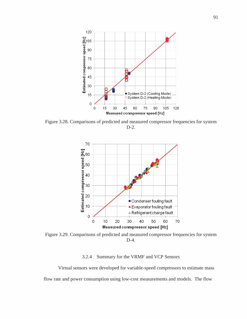
91

Figure 3.28. Comparisons of predicted and measured compressor frequencies for system

D-2.

Figure 3.29. Comparisons of predicted and measured compressor frequencies for system

D-4.

3.2.4 Summary for the VRMF and VCP Sensors

Virtual sensors were developed for variable-speed compressors to estimate mass

flow rate and power consumption using low-cost measurements and models. The flow

92

rate and input power at a rated compressor speed are correlated in terms of condensation

and evaporation temperatures and then corrected for any operating speed using additional

correlations in terms of operating frequency. The virtual sensors predicted mass flow rate

and power consumption with RMS errors less than 6% and 4%, respectively, under

normal conditions for four different systems over a range of operating conditions in

heating and cooling modes. The virtual sensors also work well when faults are present,

except in the case of compressor valve leakage faults that lead to errors in predictions of

refrigerant flow rate. Overall, predictions of mass flow rate were about 16% higher than

measurements under compressor fault conditions. In this case, other virtual sensors for

refrigerant flow could be used to isolate this fault as described by Kim and Braun (2012c)

and in Chapter 4.

For embedded applications, motor operating frequency would be an available input.

However, for application to existing equipment in the field, compressor frequency can be

difficult to measure. An alternative would be to use another virtual refrigerant mass flow

measurement as an input to the compressor mass flow model in order to estimate

compressor frequency for use in the virtual compressor power model. This was shown to

work well using the data available in this study. The estimated frequency may be a

useful index in monitoring and diagnosing faults for the system.

93

CHAPTER 4. DEVELOPMENT AND ASSESSMENT OF ALTERNATIVE VIRTUAL SENSORS

4.1 Development and Assessment of Virtual Refrigerant Mass Flow (VRMF) Sensors

Refrigerant mass flow rate is an important measurement for monitoring

equipment performance and enabling fault detection and diagnostics. However, a

traditional mass flow meter is expensive to purchase and install. The development of a

variable-refrigerant mass flow (VRMF) sensor for a variable-speed compressor is

presented in chapter 3. However, additional refrigerant flow sensors are useful in

isolating different faults. In this chapter, three different virtual refrigerant mass flow

(VRMF) sensors are presented and evaluated that use mathematical models to estimate

flow rate using low cost measurements. The three approaches use: 1) a compressor map

for refrigerant mass flow rate that uses inlet pressure and temperature and outlet pressure

as inputs; 2) an energy-balance method employs a virtual sensor for power consumption

based on a compressor map; 3) semi-empirical correlations for electronic expansion valve

(EEV) and thermostatic expansion valves (TXV) that are based on an orifice equation.

The models were trained and tested using data obtained from earlier laboratory studies.

4.1.1 System Descriptions and Test Conditions

Laboratory test data was used to develop and evaluate VRMF sensors. Table 4.1

gives specifications for equipment where data were obtained through laboratory testing.

94

The systems include a water-to-water heat pump with a variable-speed

compressor, a residential air split system, and light commercial packaged systems with

fixed and variable-speed compressors. The systems used either a TXV or EEV as an

expansion device and R-22 or R-410A as a refrigerant. Some of the units included low-

side accumulators.

Table 4.2 presents the range of operating test conditions for each unit, including

the range of refrigerant flow rates encountered. The laboratory test data were obtained

with variations in both indoor and ambient temperature. Three of four systems were

tested with different condenser and evaporator airflow rates, which could represent faults

associated with a dirty air filter or coil fouling. All of the systems except for system E-2

were tested at different refrigerant charge levels to simulate improper charge service and

refrigerant leakage. Systems E-1 and E-3 included simulated compressor valve leakage

faults where a portion of the discharge flow from the compressor was bypassed to the

compressor suction. System E-2 was a laboratory setup for testing electronic expansion

valves over a very wide range of refrigerant flows. Two different valves (B0B and B1F in

the Table 4.1) were tested with two different refrigerants (R-410A and R-404A in Table

4.2). The B1F valve has a rated refrigerant flow (also cooling capacity and associated

air/water flow) that is three times higher than that for the B0B valve with a 10 bar

pressure difference across the maximum valve opening, based on the specification in the

manufacturer’s catalog. During the course of testing for system E-2, it was discovered

that the compressor was not operating normally and was delivering significantly less than

the rated flow. Thus, this data set could also be used to represent faulty compressor

behavior. System E-3 also included fault testing for a liquid line restriction (additional

95

pressure drop increase through liquid line) and the presence of non-condensable gas

(injection of nitrogen gas into the system). In general, only normal operating (i.e., no-

fault) data were used to learn parameters of the VRMF sensors, whereas all of the data

were used for assessing VRMF sensor performance.

Table 4.1. System descriptions for laboratory test data.

System Size (kW) Refrigerant Compressor Expansion

Device Accumulat

or System Type

E-1 Kim (2005) 3 R-22 Variable-speed

compressor EEV No Water to

Water E-2 Bach (2010) 7.0 R-410A

R-404A Fixed-speed compressors

EEV (B0B/B1F) Yes

E-3 Payne (2008) 8.8 R-410A TXV Yes

Air Split Type

Table 4.2. Test conditions for laboratory test data.

System Indoor

Temperature Ambient temperature

Percentage of refrigerant

mass flow rate

Indoor air/water flow rate

Outdoor air/water flow rate

Refrigerant charge Dry Wet

( C ) ( C) ( F ) [ % ] [ % ] [%] [ % ] E-1 26.7 - 15/24/32/4

0 65~100 35~100 25~100 60~100

E-2 26.7 - 35 / 28 20~100(R410A) 10~100(R404A) 100 100 100

E-3 26.7/21

19/15/Dry 28/ 35/ 39 60~100 70~100 50~100

Coil Block 70~130

4.1.2 VRMF sensor I based on Compressor Flow Map

4.1.2.1 Development of VRMF Sensor I

A compressor map is used to estimate refrigerant mass flow rate using input

measurements of the compressor of inlet and outlet pressure. Based on ARI Standard

540(2004), the refrigerant mass flow rate for a fixed-speed compressor can be

96

represented using a 10-coefficient polynomial equation for a specified amount of

superheat. The map at the specified superheat is typically corrected using the ratio of the

compressor suction density at the actual superheat to the density at the tested superheat.

Based on the ARI model form, VRMF Sensor I for a fixed-speed compressor is

determined as

ecceeecceeccsucmap TTaTTaTaTaTTaTaTaTaTaam 29

28

37

365

24

23210 (4-1)

where mmap is the estimated refrigerant mass flow rate, the a’s are empirical coefficients,

Te is the evaporating saturation temperature, Tc is the condensing saturation temperature,

and ρsuc is the density at the suction (inlet) of the compressor.

The development of VRMF sensor I for a variable-speed compressor is explained

in chapter 3. Equation 4-1 is used to map the mass flow rate for a rated frequency and this

is corrected for other frequencies using a second-order polynomial as given in equation 4-

2. The c and b coefficients are estimated using a regression analysis applied to

experimental data.

frequencyratedcceeccratedratedsucmap TTbTbTbTbTbbcffcffcm ,52

42

3210322

1 (4-2)

where the b’s and c’s are empirical coefficients, f is compressor frequency, and frated is the

rated compressor frequency.

4.1.2.2 Performance of VRMF Sensor I

Figures 4.1 and 4.2 show the performance of VRMF sensor I that is based on a

compressor map. The terms “Normal”, “Comp Fault”, “Cond Fault”, “Evap Fault”,

“Liquid Fault”, “Charge Fault”, and “NonCond Fault” stand for no fault, compressor

97

leakage fault, condenser fouling fault, evaporator fouling fault, liquid-line restriction fault,

refrigerant leakage fault, and non-condensable gas fault, respectively. To evaluate the

performance of the VRMF sensor, the predicted ratio of refrigerant mass flow rate to the

rated flow is compared to the value determined using measurements. The parameters of

the VRMF models were trained using only the normal data, however these models were

used to predict flow rates for all of the fault tests.

Figure 4.1 shows the performance of VRMF sensor I for system E-3 with a fixed-

speed compressor under no-fault and various faulty conditions. The RMS error is

generally less than 2% for normal operation and with a variety of faults, except for

compressor valve leakage. For the range of compressor leakage conditions considered,

the RMS error for VRMF sensor I was 19%. In general, the error increases with the

severity of the compressor leakage fault. As a result, the compressor refrigerant flow map

model only provides an accurate estimation when the compressor operates normally. The

differences between refrigerant flows determined using VRMF sensor I and other VRMF

sensors can be used to diagnose a fault associated with the compressor not delivering the

proper refrigerant flow.

Figure 4.2 shows the performance of VRMF sensor I for system E-3 with a

variable-speed compressor under no-fault and various fault conditions. Although the

VRMF sensor I was trained using only no-fault data, it accurately estimates mass flow

rate for faulty conditions over the range of operating frequencies, except for the

compressor valve leakage fault. The RMS errors for VRMF sensor I were less than 3%

for condenser fouling, refrigerant charge, and evaporator fouling conditions. However,

98

VRMF sensor I predictions were about 16% higher than measurements for the range of

compressor fault conditions considered, with even greater errors at increasing fault levels.

Figure 4.1. Performance of VRMF sensor I based on a fixed-speed compressor map for system E-3 under no-fault and fault conditions (RMS of sensor errors is shown for each

fault type).

Figure 4.2. Performance of VRMF sensor I based on a variable-speed compressor map for system E-1 under no-fault and fault conditions (RMS of sensor errors is shown for

each fault type).

99

4.1.3 VRMF sensor II based on Compressor Energy Balance

4.1.3.1 Development of VRMF Sensor II

In order to diagnose compressor flow problems, it is necessary to have an

alternative VRMF sensor. One alternative approach is to use an energy balance on the

compressor to estimate the flow rate as shown in equation 4-3. Li (2006) demonstrated

that this method provides accurate flow predictions when using a virtual compressor

sensor for power consumption, even in the presence of a compressor valve leakage fault

or other faults. Compared to the map-based method, the energy balance model is much

simpler and can be used for both fixed-speed and variable-speed compressors.

),(),(1

sucsucsucdisdisdis

lossenergy PThPTh

Wm

(4-3)

where αloss is the compressor heat loss ratio, W is compressor power consumption, and

hdis(Tdis,Pdis) and hsuc(Tsuc,Psuc) are the discharge line and suction line refrigerant

enthalpies. The compressor power consumption, discharge pressure (Pdis) and suction

pressure (Psuc) can be estimated using other virtual sensors.

αloss is generally very small (under 5%) for equipment having a fixed-speed

compressor under normal operation. However, it can be more significant at low

compressor speeds for variable-speed equipment or with faults for fixed-speed equipment.

For example, decreasing the compressor frequency from 60Hz to 30Hz almost doubles

the heat loss as a fraction of the power input. To provide more accurate mass flow rate

predictions under various faulty conditions and/or speeds, an empirical model for αloss

was developed that is trained using regression applied to data. The model for fixed-speed

100

equipment is given in equation 4-4, while a function for variable-speed equipment is

shown in equation 4-5.

sucdissucdispredloss TcTcPcPcc 43210, . (4-4)

fcTcTcPcPcc sucdissucdispredloss 543210, . (4-5)

The c’s are empirical coefficients, Psuc is the suction pressure, Pdis is the discharge

pressure, Tdis is the compressor discharge temperature, Tsuc is the suction temperature, and

f is the speed of the compressor motor.

4.1.3.2 Performance of VRMF Sensor II

Figure 4.3 shows the performance of VRMF sensor II for system E-3 with a

fixed-speed compressor. The mass flow rate prediction was determined using heat loss

estimates and predictions of other virtual sensors. The heat loss model was determined

using data for normal operation where the heat loss was computed from an energy

balance on the compressor with the flow measured. The power consumption was

determined using a map in terms of suction pressure and temperature and discharge

pressure. The RMS error for the VRMF sensor was less than 3% for all of the data,

including both normal and faulty conditions. The larger errors for the evaporator fouling

occurred when the superheat at the compressor inlet was below 1.5F. The incorrect

compressor suction enthalpy due to a two-phase refrigerant inlet state led to the

inaccurate estimate of the mass flow rate. VRMF sensor II is relatively independent of

compressor faults compared to the VRMF sensor I.

101

Figure 4.4 shows the performance of VRMF sensor II for system E-1 with a

variable-speed compressor. The mass flow rate estimates were compared to

measurements for a range of different faults at different fault levels. The RMS error for

VRMF sensor II is less than 5%. Except for several low compressor speed conditions, the

VRMF works well regardless of the fault conditions. However, there were some

significant errors (10%) at low frequencies. Additional work is necessary to accurately

determine the heat loss for variable-speed compressors when operating at low frequencies.

Figure 4.3. Performance of VRMF sensor II based on an energy balance for system E-3 under no fault and fault conditions (RMS of errors is shown for each fault type).

102

Figure 4.4. Performance of VRMF sensor II based on an energy balance for system E-1

under no fault and fault conditions (RMS of errors is shown for each fault type).

4.1.4 VRMF sensor III based on Expansion Valve Model

Expansion devices are used to drop the pressure of the refrigerant and to regulate

the refrigerant mass flow rate in response to a variable load. There are three types of

expansion devices used in air conditioners: fixed-orifice (FXO), thermostatic expansion

valve (TXV), and electronic expansion valve (EEV). Even though an FXO has

advantages of simplicity and low cost, it is not appropriate for a system that requires

precise flow control for a wide range of flow rate requirements. TXV and EEV devices

are both expansion valves that have an adjustable throat-area. The TXV adopts a

mechanical control method to obtain relatively constant superheat at the evaporator outlet.

The EEV provides a more precise control of superheat and fast flow control for a wide

range of mass flow rates because it uses electronic actuation and sensor information

along with a digital feedback controller. Most of the previous literature on modeling of

expansion devices has focused on constant-area expansion devices, such as FXOs.

103

Models for predicting the mass flow characteristics of TXVs and EEVs are limited. Li

(2008) developed generalized expressions for TXV mass flow rate as a function of

superheat. Shanwei et al. (2005) and Park et al. (2007) developed empirical correlations

for mass flow rate through an EEV by performing a dimensionless analysis based on a

power law form. However, these existing models require either detailed geometric

parameters or many measurements to represent valve performance. This thesis presents

VRMF sensors for TXV and EEV devices based on a semi-empirical model that can be

trained using a relatively small amount of data and then can estimate refrigerant mass

flow rate as part of an automated diagnostic system.

4.1.4.1 Development of VRMF Sensor III for TXVs

Expansion devices are used to drop the pressure of the refrigerant and to regulate

the refrigerant mass flow rate in response to a variable load. The TXV adopts a

mechanical control method to obtain relatively constant superheat at the evaporator outlet.

The valve opening for a TXV is determined by a force balance on a diaphragm, as

depicted in Figure 4.5. The bulb and suction-line pressure act on opposite sides of the

diaphragm and coupled with the spring force, control the effective orifice area. The

evaporator inlet and condenser pressure influence the flow rate through the orifice for a

given opening. The bulb typically contains a two-phase mixture of the same refrigerant

that is employed within the system. Therefore, when a positive superheat exists at the

evaporator outlet then there is a positive difference between the bulb and evaporator

outlet pressures acting on the diaphragm. The spring is used to ensure a positive

104

superheat at the evaporator exit since the bulb pressure must be greater than the

evaporator exit pressure in order to overcome the force of the spring.

As depicted in Figure 4.5, a conical pin moves up and down to change the open

area for refrigerant flow in response to the valve control. The mass flow rate through the

TXV is assumed to be a linear function of the open area as given in

maxmA

AAm

orifice

pinorificeTXV (4-6)

where Aorifice= ((Dorifice)2·π)/4 is the area at the full opening, Apin= ((Dpin)2·π)/4 is the

closed area associated with the pin and mmax is the refrigerant mass flow rate associated

with a full open condition.

Figure 4.5. Diagram of a TXV.

The maximum flow rate for a given valve is a function of the pressure drop across

the valve and the size of the orifice. The maximum flow rate for a given orifice is

calculated using the empirical correlation given in equations 4-7 and 4-8, as developed by

Hrnjak (1998).

105

KPPCKPPACm ecfecforifice 22 10max (4-7)

54

2

12 C

PPP

CT

SCCKcri

ecri

C

cri

(4-8)

where the C’s are empirical coefficients, (Pc-Pe) is the difference between the valve inlet

pressure and the evaporating pressure, ρf is the density of the refrigerant at the valve inlet,

SC is the subcooling of the refrigerant at the valve inlet, Tcri and Pcri are the critical

temperature and pressure.

The spring deflection, δsp needs to be known in order to find the effective orifice

area. The deflection of the spring can be found as

sp

clspspsp k

FF , (4-9)

where Fsp is the spring force, Fsp,cl is the spring force when the valve is closed and ksp is

the spring constant. Both Fsp,cl and ksp are fixed for a given expansion valve. Fsp is

calculated from a quasi-static force balance on the diaphragm, as shown in

sucediaphsucbdiaphsp PPAPPAF (4-10)

where (Pb-Psuc) is the pressure difference between bulb and suction line, and Adiaph is the

area of the diaphragm. Fsp,cl, Adiaph and ksp are constants based on the valve design and

initial setting.

Since the spring force is a linear function of the deflection, the spring deflection

can be expressed using empirical coefficients (a’s), as shown in

21, aPPa

kFPPA

sucesp

clspsucediaphsp (4-11)

106

If the pin deflection is zero, no refrigerant flows through the orifice, and if the pin

deflection is at some maximum value, the pin will not obstruct the flow and the valve will

operate at the maximum flow rate. The effective orifice area is calculated by subtracting

the obstructing area of the pin from the area of the valve orifice. The VRMF sensor for a

TXV is developed by substituting δsp from equation 4-11 into equation 4-6 and

expressing the result in terms of new empirical coefficients that are determined through

regression.

max2

2max22

maxmax 44mCmm

AAA

m spsporifice

pinorificeTXV

.

KPPCaPPaPPam ecfsucesuceTXV 21542

3 . (4-12)

4.1.4.2 Performance of VRMF Sensor III for TXVs

The empirical coefficients C1, C2, C3, C4 and C5 within orifice equations 4-7 and

4-8 were estimated by minimizing mass flow rate prediction errors using fully open TXV

test data and non-linear regression. Fully open TXV test data were collected from the

conditions where the superheat of the compressor inlet was higher than the rated

superheat. The empirical coefficients a3, a4, and a5 within the TXV model equation 4-12

were estimated based on the available normal test data with superheat under control using

linear regression. The data includes variations in ambient temperature, and indoor dry

bulb temperature with positive subcooling entering the valve. Since equation 4-8 uses

subcooling as an input, zero subcooling data were disregarded for training and testing.

The parameter estimation methods minimized the errors between predicted and known

107

mass flow rates. The resulting model with empirical coefficients determined from normal

data was applied to predict refrigerant mass flow rates for all of the available data

including various fault conditions.

Figure 4.6 shows the refrigerant mass flow rate estimated from the VRMF sensor

III for a TXV applied to system E-3 with six different kinds of faults individually

implemented. The overall RMS errors were about 1% for no-fault conditions and 3% of

the actual mass flow rate for all fault conditions. The performance of the VRMF sensor is

very good over a wide range of refrigerant mass flow rates and operating conditions

regardless of the fault. There were some significant errors of about 10% for low

refrigerant charge levels when the entering subcooling was almost zero. With zero

subcooling and two-phase conditions entering the TXV, VRMF sensor III may not be

reliable.

Figure 4.6. Performance of VRMF sensor III based on a TXV model for system E-3 under no-fault and fault conditions (RMS of sensor errors is shown for each fault type).

108

4.1.4.3 Development of VRMF Sensor III for EEV

Electronic expansion valves (EEV) were developed in the 1980s to provide tighter

and more stable control of superheat with faster response. The applications of EEVs for

high efficiency air conditioner and multi-evaporator heat pump systems have increased in

recent years. However, mass flow models of EEVs for fault detection and diagnosis are

very limited. In this study, the VRMF sensor based on an empirical correlation, which

can predict refrigerant mass flow rates through an EEV, is described.

The empirical mass flow correlation was developed by incorporating a

dimensionless coefficient in terms of EEV geometries and operating conditions into the

orifice equations 4- 6 and 4-7. This is done because the only difference between the EEV

and the TXV model is how the area opens and closes. The empirical correlation for

VRMF sensor is given in

KPPCD

mAm ecfactual

actualEEV 24 1

2

max (4-13)

where the C’s are empirical coefficients, Dactual is the actual orifice diameter (see Figure

4.7), ρf is the density of refrigerant at the valve inlet, Pc and Pe are the inlet pressure and

evaporator pressure. The variation of the actual orifice diameter controls the refrigerant

flow area for flow restriction. The mass flow rate proportionally increases with the rise of

the flow area.

Figure 4.7 shows the flow passage structure and geometric representation for an

EEV. A needle valve moves up and down to change the flow area, typically using a

stepper motor to maintain precise control of the refrigerant superheat at the evaporator

exit. At a certain pin tip position h, the refrigerant flow area Aactual can be calculated by

109

subtracting the obstructing area of the needle from the area of the valve orifice as

developed by Li (2008) and given in

22222

tan2444

hHDDDD

A orificepinorificeactual

actual (4-14)

where Dpin=(2·tanθ·(H-h)) is the current needle diameter that is within the plane of the

flow orifice, and Dorifice=2·H·tanθ is the orifice diameter.

Figure 4.7. Flow passage structure and geometric models for EEV.

The current needle diameter can then be expressed in terms of the orifice diameter

and needle position as shown in

HhDhH

HD

D orificeorifice

pin 12

2 . (4-15)

Equations 4-14 and 4-15 can be combined to express the refrigerant flow area,

Aactual, for any needle position, as

Hh

HhD

Hh

HhDDA orificeorificeorificeactual 2

421

42

222 . (4-16)

110

The refrigerant mass flow rate through the EEV can be obtained by substituting

the refrigerant flow area, equation 4-16, into the general model equation 4-13.

KPPHh

HhD

Cm ecforifice

EEV 224

2

1 . (4-17)

The flow area of the EEV varies with the up-and-down movement of the needle

valve that is driven by a stepper motor. The needle position (h) is linearly proportional to

the motor step of the EEV, as given in

HEEVSTEP

EEVSTEPh current

max

. (4-18)

In this study, the VRMF sensor for an EEV was developed by substituting the

ratio of motor step, equation 4-18, into the EEV refrigerant mass flow rate equation 4-17.

The coefficients D1 and D2 in equation 4-19 can be determined using linear regression

based on normal test data.

max0max

2

max 224

mHh

HhDm

Hh

HhD

mA

AAm orifice

orifice

pinorificeEEV

KPPCEEVSTEP

EEVSTEPDEEVSTEP

EEVSTEPDm ecfcurrentcurrent

EEV 21max

2

2

max1

(4-19)

4.1.4.4 Performance of VRMF Sensor III for EEVs

The empirical coefficients within orifice equation 4-7 were determined using non-

linear regression applied to data in which the EEV fully open. These data were collected

from the conditions where the motor step was at a maximum. Like the TXV, equation 4-8

uses subcooling as in input, and thus zero subcooling data were disregarded for training

111

and testing. Once the empirical coefficients of the orifice equation are obtained, the EEV

equation 4-19 is fit to normal operating (i.e., no-fault) data using linear regression.

Figure 4.8 shows the performance of the VRMF sensor III for EEV approach

applied to system E-1. The model provides results that are generally within 6% over a

wide range of mass flow rates and operating conditions. Larger errors for low refrigerant

charge and condenser fouling occurred when the subcooling at the condenser outlet was

below 2 F. The best fit equation was then used to predict the refrigerant mass flow rate

through the EEV for all available test data including various fault conditions.

Figure 4.8. Performance of VRMF sensor III based on EEV for system E-1 under no fault

and fault conditions (RMS of sensor errors shown for each fault type).

Figures 4.9 and 4.10 show performance of VRMF sensor III with an EEV applied

to system E-2 with R-410A and R-404A as the refrigerant. Results are presented for two

different EEVs that were tested in this system. Overall, the RMS errors of the VRMF

sensor III were 6% and 5% for R-410A and R-404A, respectively. Some of the larger

112

errors may be associated with two-phase refrigerant conditions at the EEV inlet with

near-zero subcooling.

Figure 4.9. Performance of VRMF sensor III based on EEV with R410a as refrigerant for

system E-2.


for system E-2.

113

4.1.5 Application of VRMF Sensors for Fault Detection and Diagnosis

The application of the virtual sensors for diagnosing compressor valve faults and

their insensitivity to other faults are demonstrated using the available data. When a

compressor suction or discharge valve is leaking and the compressor is not delivering the

expected flow, the energy-balance or EEV model can provide accurate flow estimates. In

this case, the flow differences provide an indication of loss of compressor performance

and can be used for fault detection and diagnostics.

Outputs from the three VRMF sensors can be compared in order to detect a fault

and localize faults within a system, including 1) loss of compressor performance, 2)

faulty compressor motor, and 3) faulty expansion device. Figures 4.11 to 4.13

demonstrate the use of the VRMF sensors for isolating a fault condition where the

compressor is not providing the expected flow.

Figure 4.11 shows comparisons of the three VRMF sensors with mass flow

measurements for system E-3 operating at fixed-speed with a simulated compressor valve

leakage fault. With this fault, the refrigerant mass flow rate is reduced compared to

normal operation. As a result, the compressor map over-predicts the refrigerant mass flow

rate whereas the other VRMF sensors provide accurate flow estimates. The RMS errors

for the compressor energy balance model and TXV models were about 2%, whereas the

RMS error for the fixed-speed compressor model was 19%. Thus, a compressor flow

fault could be isolated through comparison of the VRMF sensors for this case.

Figure 4.12 shows similar results for system E-1 having a variable-speed

compressor and EEV. The RMS errors for the VRMF sensors were about 5% based on a

114

compressor energy balance and 3% based on the EEV model. However, they were

approximately 16% for the variable-speed compressor map.

Figures 4.13 and 4.14 Figures 4.13 and 4.14 show the results for system E-2 with

B1F and B0B as expansion devices and the two different refrigerant types, R-410A and

R-404a. The data did not include information that could be used to evaluate the energy

balance method. The tests covered a wide range of compressor fault levels from 10 to

100%. For either set of test data, a compressor fault could be readily identified by

comparing predictions of the compressor map with those from the EEV model.

Figure 4.11. Comparison of VRMF sensor outputs for system E-3 with a compressor flow

fault.

115

Figure 4.12. Comparison of VRMF sensor outputs for system E-1 with a compressor flow

fault.


compressor flow fault.

116


compressor flow fault.

4.1.6 Summary for Alternative VRMF Sensors

Refrigerant mass flow rate is an important measurement for equipment

performance monitoring, fault detection, and diagnostics. However, a typical refrigerant

mass flow meter is expensive. In addition, installation for existing field equipment is

complicated because it requires an equipment modification that can lead to refrigerant

leakage. To enable low-cost implementations for on-line performance monitoring and

automated diagnostics, three different virtual refrigerant mass flow (VRMF) sensors were

developed. Each sensor estimates the refrigerant mass flow rate from low-cost

measurements that are based on: 1) a compressor map, 2) a compressor energy balance,

and 3) a semi-empirical correlation for the expansion device (TXV or EEV).

The VRMF sensors presented were validated for systems having fixed and

variable-speed compressors, different refrigerants, and different expansion devices

(TXV/EXV) over a wide range of operating conditions both with and without faults. The

117

three VRMFs work well in estimating the refrigerant mass flow rate for the various

systems under fault-free conditions with less than 5% RMS error. Predictions from the

VRMF sensor based on a compressor map deviate from the other VRMF sensors in the

presence of a compressor fault with the deviations growing with the magnitude of the

fault. These differences can be used within a diagnostic system to isolate this particular

fault since the accuracy of the energy balance model and expansion device models is

independent of compressor flow faults.

4.2 Development and Assessment of a Virtual Air Flow (VAF) and Virtual Heat

Exchanger Conductance (VHXC) Sensor

4.2.1 VAF and VHXC Sensors for Condensers

Fouling of air side heat exchangers, the deposition of dust and other particulate

matter, increases system pressure drop and, correspondingly, decreases system air flow

and air conditioner performance. Fouling can also impact air-side heat transfer

coefficients by providing an insulating resistance. Based on previous work by Li et al.

(2007), the reduction of air flow rate due to increased pressure drop dominates the effect

of increased thermal resistance due to a fouling layer.

118

Figure 4.15. Virtual sensor for condensers using 1) energy balance and 2) overall

condenser conductance.

In order to detect fouling faults for condensers, two virtual sensors were

developed that are depicted in Figure 4.15. First, the condenser air flow rate can be

estimated using an energy balance that includes both air and refrigerant flow streams.

Second, an overall condenser heat transfer conductance, UAcond , is estimated as a feature

to diagnose condenser fouling faults.

4.2.1.1 Virtual Sensor for Condensers based on an Energy Balance

To diagnosis condenser fouling conditions, a virtual sensor for condenser air flow

rate is employed for systems having a fixed-speed condenser fan. Air flow measurements

are generally very expensive and unreliable for application in the field. Air flow rates can

be estimated using energy balances on the condenser as expressed in

condairP

acond

icaoca

inliinliinliquiddisdisdisrefpredicted C

vTT

TPhTPhmV

,,

,

,,

,,, ,, (4-20)

119

where Vpredicted is the condenser air volume flow rate, vcond,a is the condenser air specific

volume, Cp,air,cond is the air specific heat, Ta,oc is the condenser outlet air temperature, Ta,ic

is the condenser inlet air temperature, mref is the refrigerant mass flow rate provided from

the VRMF sensor, hdis is the discharge line refrigerant enthalpy, Pdis is the discharge line

pressure, Tdis the is discharge line temperature, hli,in is the liquid-line refrigerant enthalpy,

Pli,in and Tli,in are the liquid-line pressure and temperature.

The predicted air flow rate can be compared to a target air flow rate to detect

fouling. The target flow can be obtained from a manufacturer’s catalog or from a normal

value when the FDD scheme is implemented assuming that there is no fouling. The

energy balance model has the limitation of not being valid when subcooling at the outlet

of the condenser is zero. However, zero subcooling is typically associated with low

refrigerant charge, which can be diagnosed using the VRC sensor.

Figure 4.16 shows the condenser air flow rate estimated from the VAF sensor for

system E-3 with normal and faulty conditions. Overall, the VAF sensor predicted the

target condenser air flow rate, 1300 [CFM], within 3 % except under condenser fouling

fault conditions. As the severity of the condenser fouling increases, the estimated air flow

rate is decreased. Condenser air flow rate reduction is an independent feature for

condenser fouling. It also is a good feature for diagnosing condenser fan problems.

120

Figure 4.16. Predicted condenser air flow from an energy balance versus expected value

for system E-3.

4.2.1.2 Virtual Sensor for Condenser based on UA

According to Reddy (2006), heat exchanger conductance, UAcond, is an important

feature for diagnosing condenser fouling. As the severity level of the condenser fouling

fault increases, the UAcond value should decrease. The value of UAcond is estimated from

measurements and other virtual sensor outputs using

satcica

satcoca

ocaicapredictedcondinliinliinliquiddisdisdisrefcond

TTTT

LN

TTUATPhTPhmQ

,,

,,

,,,,,, ,, (4-21)

where Qcond is the condenser refrigerant side capacity and Tc,sat is the condenser saturation

temperature. UAcond is dependent on refrigerant mass flow rates and operating conditions.

Therefore, it is necessary to determine a model for these variations in the absence of

condenser fouling in order to enable fault detection and diagnostics.

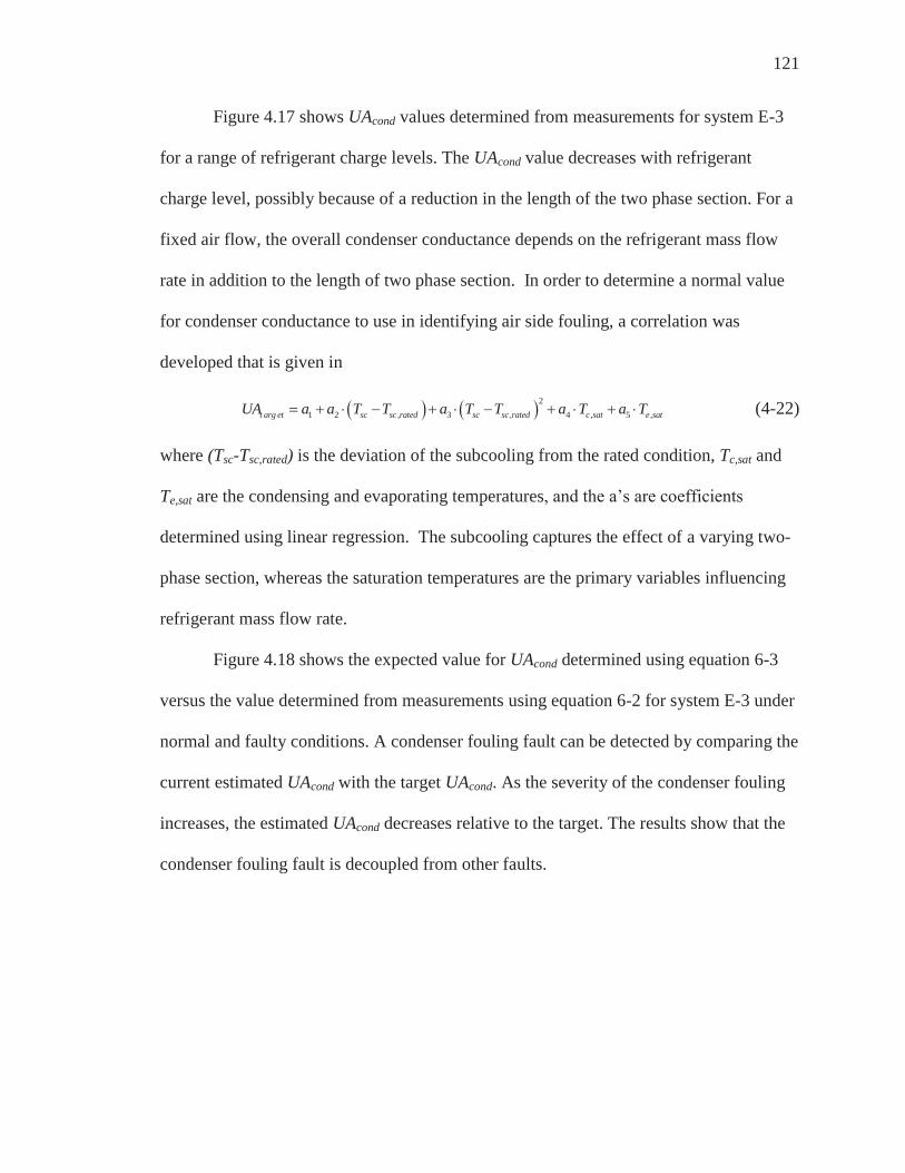
121

Figure 4.17 shows UAcond values determined from measurements for system E-3

for a range of refrigerant charge levels. The UAcond value decreases with refrigerant

charge level, possibly because of a reduction in the length of the two phase section. For a

fixed air flow, the overall condenser conductance depends on the refrigerant mass flow

rate in addition to the length of two phase section. In order to determine a normal value

for condenser conductance to use in identifying air side fouling, a correlation was

developed that is given in

21 2 3 4 5t arg et sc sc,rated sc sc,rated c,sat e,satUA a a T T a T T a T a T (4-22)

where (Tsc-Tsc,rated) is the deviation of the subcooling from the rated condition, Tc,sat and

Te,sat are the condensing and evaporating temperatures, and the a’s are coefficients

determined using linear regression. The subcooling captures the effect of a varying two-

phase section, whereas the saturation temperatures are the primary variables influencing

refrigerant mass flow rate.

Figure 4.18 shows the expected value for UAcond determined using equation 6-3

versus the value determined from measurements using equation 6-2 for system E-3 under

normal and faulty conditions. A condenser fouling fault can be detected by comparing the

current estimated UAcond with the target UAcond. As the severity of the condenser fouling

increases, the estimated UAcond decreases relative to the target. The results show that the

condenser fouling fault is decoupled from other faults.

122

Figure 4.17. Calculated UAcond as a function of deviation from normal charge for system

E-3.

Figure 4.18. Expected UAcond versus UAcond determined from measurements for system

E-3.

4.2.2 VAF and VHXC Sensor for Evaporator

Two virtual sensors were developed for evaporators that estimate air flow rate and

overall energy transfer conductance. The development approach is similar to the

123

approach described for condensers in the previous section. Figure 4.19 illustrates the

VAF sensor module for evaporators.

Figure 4.19. VAF sensor for evaporators using 1) energy balance and 2) overall

conductance.

4.2.2.1 Virtual sensor for evaporators based on an energy balance

Evaporator air flow is estimated from an energy balance using equation 4-23,

oeaiea

aevapinevapinevapinevapoutevapoutevapoutevaprefevappredicted hh

vTPhTPhmV

,,

,,,,,,,,

,, (4-23)

where Vpredicted,evap is the evaporator air volume flow rate, vevap,a is the evaporator air

specific volume, ha,ie is the evaporator inlet air enthalpy, ha,oe is the evaporator outlet air

enthalpy, mref is the refrigerant mass flow rate provided from a VRMF sensor, hevap,out and

hevap,in are the evaporator refrigerant outlet and inlet enthalpies, Pevap,o and Tevap,o are the

evaporator refrigerant outlet pressure and temperature.

124

The indoor unit typically has more than one speed setting, but the air flow is

constant for a given setting. Therefore, the virtual sensor can be used to estimate the air

flow rate for each fan setting and compare with a target air flow rate.

Figure 4.20 shows the accuracy of the air flow prediction from an energy balance

for system E-3 with normal and faulty operation. The overall RMS error is about 3%. As

the fault level of evaporator fouling increased, there was a bigger difference between the

estimated and normal air flow rate of 1000 CFM.

Figure 4.20. Predicted evaporator air flow from an energy balance versus expected value

for system E-3.

4.2.2.2 Virtual sensor for evaporators based on UA

An evaporator energy transfer conductance, UAevap, is estimated from

measurements and other virtual sensor outputs using

sateiea

sateoea

oeaieapredictedevapinliquidinliquidinliquidsucsucsucrefevap

TTTT

LN

hhUATPhTPhmQ

,,

,,

,,,,,, ,,

(4-24)

125

where Qevap is the evaporator refrigerant side capacity and Te,sat is the evaporator

saturation temperature.

Figure 4.21 shows values of UAevap determined using equation 4-24 as a function

of refrigerant charge. Similar to UAcond, the estimated UAevap is dependent on refrigerant

charge level, but in this case it increases with increasing charge level. In general, the

overall conductance depends on the refrigerant flow rate in addition to the length of the

two phase section. In order to determine a normal value for evaporator conductance to

use in identifying air side fouling, a correlation was developed that is given in

21 2 3 4 5t arg et sh sh,rated sh sh,rated e,sat c,satUA a a T T a T T a T a T (4-25)

where, (Tsh-Tsh,rated) is the deviation of the superheat from the rated condition and the a’s

are coefficients determined using linear regression The superheat captures the effect of a

varying two phase section, whereas the saturation temperatures are the primary variables

influencing refrigerant mass flow rate.

Figure 4.22 shows the expected values for evaporator conductance versus the

output from the virtual sensor for conductance applied to system E-3 under normal and

faulty conditions. The difference between the prediction and measurement is proportional

to the evaporator fault level. As the fault level of the evaporator fouling increases, the

UAevap value is reduced. UAevap is a good indicator for detecting and diagnosing

evaporator fouling faults.

126

Figure 4.21. Calculated UAevap as a function of deviation from normal charge for system

E-3.

Figure 4.22. Expected UAevap versus UAevap determined from measurements for system

E-3.

127

CHAPTER 5. STRUCTURE FOR A DIAGNOSTIC DECISION SYSTEM

The primary objective of this chapter is to present a structure for a diagnostic

decision support system for air conditioning equipment. The proposed FDD system is

based on the use of virtual sensors as depicted in the block diagram of Figure 5.1. The

FDD method is broken down into four steps: preprocessor, fault detection, fault diagnosis,

and decision.

Figure 5.1. FDD block diagram for RTUs.

128

In the preprocessor block, transient input and output measurements are filtered out

using a steady state detector. Once measurements are collected, a fault detection step is

used to determine if a fault has occurred. The FDD detection uses three types of virtual

sensors; sensor level, component level, and system level. The outputs of the virtual

sensors are processed by a fault classifier which compares outputs from the virtual

sensors to expected values associated with normal behavior to evaluate whether a fault is

present. The fault diagnosis block determines the cause of the fault from a list of

possibilities. Once, the existence of a fault has been detected and identified, a decision

block recommends the proper maintenance needed based upon economic considerations.

The virtual sensors can be divided into three classes, sensor-level, component-

level, and system-level as depicted in Figure 5.2. The sensor level provides virtual

sensors that replace real measurements (e.g. refrigerant pressure) using lower cost

measurements (refrigerant saturation temperature) and correlations that do not depend on

component performance (e.g. refrigerant property correlations). The component level

sensors utilize component models (e.g. compressor maps) and low cost measurements to

determine quantities (e.g. refrigerant mass flow rate) that can be used for fault detection

and diagnosis and as inputs to evaluate fault impacts. In order to be useful for isolating

fault sources, these component level virtual sensors should provide outputs that are only

influenced by individual faults within that component (e.g. compressor mass flow and

valve leakage). System level virtual sensors provide outputs for quantities that could not

be determined solely using component level information, including overall refrigerant

charge, cooling or heating capacity, and COP.

129

Figure 5.2. Virtual sensor classifications for air conditioners.

Widespread application of virtual sensors in air conditioning equipment would

require an integrated, on-line performance monitoring and diagnostic system. To achieve

an integrated system, the virtual sensors should have linkages with shared outputs and

inputs, and provide real-time information about capacity, power consumption, and energy

efficiency for assessing economic impact. Figure 5.3 shows an example of the inter-

relationships between real and virtual sensors within an integrated FDD system for air

conditioning equipment. Sensor-level virtual pressure sensors estimate condensing and

evaporating pressures using saturation temperature measurements and property relations.

A component level virtual sensor for refrigerant flow rate uses the outputs of the virtual

pressure sensors and a component model. The output of the derived virtual refrigerant

flow sensor is used for input to a system level sensor (virtual performance sensor) to

calculate COP or EER.

130

Figure 5.3. Example of virtual sensor interactions for air conditioning equipment.

5.1 Steady State Detector for Preprocessor

A steady-state detector is used to filter out transient data, since the virtual sensors

are based on steady-state operating conditions. A combined slope and variance steady-

state detection algorithm (Li and Braun, 2003) is used. This algorithm uses a fixed-length

sliding window of recent measurements to compute the slope (k) of the best-fit line

shown in Equation 5-1 and standard deviation about the mean shown in Equation 5-2. If

both the slope and standard deviation for the sliding window are smaller than

corresponding thresholds, the system is assumed to be in a quasi-steady condition. The

sliding window is specified by the number (n) of data points (ym, ym+1… ym+n-1) and

sampling time (τ).

A small threshold leads to more stable states, but less input data for FDD. On the

other hand, large thresholds increase the uncertainty of the FDD outputs. Therefore, it is

necessary to find thresholds that minimize the uncertainty of the FDD system while

maximizing the use of input data.

( ) , , 1,..., 1iy a k i m i m m m n . (5-1)

131

1 121 1( )

m n m n

i ii m i m

S y yn n . (5-2)

5.2 Fault Detection

Faults can be detected by comparing fault-free expected values to current values

based on measurements, and analyzing their residuals. Virtual sensors provide estimates

of current features that can be compared to expected values for fault-free operation. A

classifier is used to determine whether the deviation between current and expected values

is statistically significant. In fault detection, estimated variables representing current

operation are classified as either normal or faulty. The residuals between outputs from

virtual sensors and expected values for normal operation are used by a fault detection

classifier. The fault detection classifier estimates the overlap between the probability

distributions of residuals for current and normal operation. In this section, a statistical

Bayesian fault detection classifier proposed by Rossi and Braun (1997), and a normalized

distance fault detection classifier presented by Li and Braun (2007b) are reviewed.

5.2.1 Bayesian Fault Detection Classifier

There are several possible statistical classifier designs for fault detection. A

parametric design was chosen over a non-parametric design because it is assumed that

measurement noise is caused by independent random processes that are normally

distributed. A Bayes decision classifier is the best choice among the parametric

classifiers. (Fukunaga,1990)

Based on Bayes decision theorem, equation 5-2 can be written as

132

xppxp

xp iii (5-3)

where p( i|x) is the conditional probability of i having accounted for evidence x. p( i)

is prior probability and P(x| i) is the class conditional probability density function. P(x)

is the mixture density function. Since P(x) is positive and common to both sides of the

inequality, the Bayes decision rule of equation 5-3 can be expressed as

22111 :)( pxppxpNormal

22112 :)( pxppxpfault (5-4)

1

2

2

1)(pp

xpxp

xl . (5-5)

The term l(x) is called the likelihood ratio and is the basic quantity in hypothesis

testing. In that case, the decision rule of equation 5-5 becomes the term h(x), which is

called the discriminant function.

1221

2

1 logloglogloglog

)(log)(

ppxpxpxpxp

xlxh

. (5-6)

Figure 5.6 shows two conditional probabilities p(x| i), i=1, 2, as functions of x in

each of the classes. The dotted line at x0 is a threshold partitioned into two regions, R1

and R2. According to the Bayes decision rule, for all x values in R1 the classifier decides

1 and for all x values in R2 it decides 2. However, there is overlapping probability

which is equal to the total shaded area under the curves belonging in R1 and R2, shown in

Error! Reference source not found.. The shaded area is the classification error

robability (ε), which is given by

133

22112211 ppdxpxpdxpxpox

ox. (5-7)

Figure 5.4. Bayes decision rule for minimum error (w1 : no fault & w2 : fault condition).

The classification error probability decreases as a fault becomes more significant

and is therefore a useful measure for detecting a fault. However, the computation of

equation 5-7 is a very complex problem due to the fact that ε is obtained by integrating

the density functions. Therefore, integrating discriminant function h(x) is more

convenient in this case.

One of the most common probability density functions in practice is the normal

probability density function. When P(x| i) is the normal distribution with mean μi and

covariance Σi, shown in equation 5-8, equation 5-9 can be expressed using

222111 ,~,,~ NxpNxp (5-8)

)2(1log

2)()(

2)()(

exp)2(

1loglog)(

1

1

i

iit

i

iit

i

iii

xx

xxxpxg

(5-9)

134

where x is a vector of current residuals, μ1 is the mean describing the distribution of

residuals and Σ1 is the covariance describing the uncertainty of residuals without faults.

μ2 is the mean describing the distribution of current residuals and Σ2 is the covariance

describing the uncertainty of current residuals.

If covariance is the same due to the symmetry of the problem, then Σ = Σ1 = Σ2.

This yields a quadratic function and equation 5-11 is a linear function of x, shown in

22

122

11

111 log

2)()(

log2

)()(P

xxP

xx tt

(5-10)

2121

211

11

12 /log21)( PPxxh ttt . (5-11)

This is the linear discriminate function shown in equation 5-12, based on 1) the

optimum coefficient tV and 2) the threshold for a given distribution 0v .

021

211

11

12 21)( vxVxxh tttt . (5-12)

The expected value and variance of h(x) can be calculated by

21

211

11

12 21)( tt

it

ii xExhE (5-13)

it

ii xExhE 11

122

12 )( . (5-14)

Since E(x| i) is mean μi, equations 5-13 and 5-14 become

121

1221

211

111

12

21

211

111

1211

21

21

21)(

tttt

ttt xExxhE (5-15)

21

211

121

1222 21)( ttt xExxhE (5-16)

135

2

)(

121

12

21

1121

21

21

t

it xxExxhE

(5-17)

2)( 22

222 xxhE (5-18)

where η is the squared Mahalanobis distance between μ1 and μ2. The Mahalanobis

distance is a good measure of separation between normal and current classes. P(h(x)| 1)

is a normal distribution with mean -η and covariance 2η, and P(h(x)| 2) is a normal

distribution with mean +η and covariance 2η.

The hatched area in Figure 5-7 corresponds to the error probabilities, which can

be expressed as

421

21

21

)()()(

221

2

21log

11211

terfde

dhxxhPxxgxgP

t

PP

t

(5-19)

42

121)()( 2122

terfxxgxgP . (5-20)

Overall, the classification error (ε) in the Bayes classifier can be calculated using

residuals with normal and fault distributions for fault detection. Equation 5-7 can be

rewritten as equation 5-21 using equation 5-19 and 20. A fault is indicated whenever the

classification error is below a threshold which is determined based on fault-free

conditions. The threshold for classification error gives a small false alarm rate and was

found to provide acceptable fault detection sensitivities

421

21

421

21

212211terfpterfppp . (5-21)

136

5.2.2 Normalized Distance Detection Classifier

Li and Braun (2007b) presented the development of a simple fault detection

classifier for both individual and multiple faults. The normalized distance classifier is

based on a one-dimensional normal distribution. The distance (d) between any point (x)

and the mean (μnormal) can be normalized by the standard deviation (σnormal), shown in

equations 5-22. Equation 5-23 indicates the maximum normalized distance (dmax)

corresponding to the given threshold (α) for false alarms by referring to a normal

distribution table. If d ≤ dmax, the system with measurement x is considered to be normal

with a confidence of 1- α. Additionally, if d ≤ dmax, then a fault is assumed with a false

alarm probability of α.

dxyprobabilitnormal

normalnormalnormal )( , . (5-22)

max, 1)( dxyprobabilitnormal

normalnormalnormal . (5-23)

The normalized distance for a multi-dimensional case X= Tnxxx 21 from

a group of values with mean (μnormal = Tn21 ) and covariance matrix normal

is defined as shown in

1)( 2max

1 dXXyprobabilit normalnormalnormal . (5-24)

The current operating distance can be calculated based on the chi-squared

distribution χ2(r). The chi-squared distribution is a special case of the gamma distribution

Γ(x), in which /r where r is a positive integer, and 2 . The continuous type

random variable X has a chi-squared distribution, with r degrees of freedom, if its

probability density function is given by follows.

137

xexr

xf xrr 0

2)2/(1)( )2/(12/

2/ . (5-25)

dxex x /1/)( /1

0 . (5-26)

Equation 5-24 can be expressed based on the chi-squared distribution.

22,,

1,, )( iinormalinormal

Tinormali drxx (5-27)

where χ2(r) is the chi-squared distribution, n is the degrees of freedom, and σ2normal = Σ-

1normal is the inverse of the normal covariance matrix.

In the residual space, operating distances located outside the normal operation are

classified as faulty conditions while operating distances located inside the normal

operation are classified as normal conditions.

5.3 Fault Diagnosis and Decision

Most of the earlier work involving FDD for air conditioning equipment has

involved the use of residuals between measurements and expected values from models

for state variables. Once a fault is detected, then a fault diagnostic classifier is employed

to find the best match between the changes in residuals and a set of rules associated with

different types of faults. One difficulty in applying this approach with a fault diagnosis

classifier is in handling multiple faults that occur simultaneously because the state

variables can depend on more than one fault along with the operating conditions as

illustrated in Figure 5.5. An FDD method should be able to decouple these effects in

order to handle multiple simultaneous faults.

138

Figure 5.5. Overall fault interactions for air conditioning equipment.

Li et al. (2007b) presented a decoupling FDD approach that relies on the use of

virtual sensors that are uniquely dependent on individual faults and decoupled from the

effects of other faults. Virtual sensors are used in place of real sensors in most cases

because the measurements required for the decoupling features would be prohibitively

expensive (e.g., refrigerant mass flow rate). With the decoupling approach, it is not

necessary to have a separate diagnostic classifier. Fault diagnoses result directly from the

identification when decoupled features deviate significantly from expected values as

determined with the fault detection classifier.

Once faults are detected and the causes of the faults are identified, proper action

should follow to fix the problems, adapt the control, or flag them for continued

monitoring. The fault impact is used to determine thresholds for the FDD system for

decision support. An assessment of the severity of the fault is essential to this decision

process and virtual sensors can be used as inputs to this analysis. If thresholds were set

139

too close to normal conditions, the FDD system would be too sensitive leading to false

alarms. If thresholds were set too far from normal conditions, the FDD system might miss

faults that potentially reduce system performance. Therefore, it is very important to

define reasonable thresholds for appropriate fault detection and diagnosis.

Capacity and energy efficiency are important information for evaluating the fault

impact for air conditioner and heat pump systems. Capacity and energy efficiency are

calculated based on virtual sensors for mass flow rate and power consumption with some

other relatively low cost temperature measurements, shown in equations 5-28 and 5-29.

An assessment of the severity of the fault is essential to this decision process and virtual

sensors for system performance can be used as inputs to this analysis. This type of

information can be used within an online tool for assessing the economics associated with

servicing a unit if faults exist.

outliquidsatcondoutliquidoutevapsatevapoutevapsorvirtualsenpredicted TPhTPhmQ ,,,,,, ,, (5-28)

sorvirtualsen

predictedpredicted W

QCOP

(5-29)

where Qpredicted, and COPpredicted are the predicted capacity and energy efficiency using the

virtual refrigerant mass flow rate ( sorvirtualsenm ) and virtual power sensors ( sorvirtualsenW ) as

inputs.

To evaluate the fault impact and assess the decision step, expected performance

models for capacity ( mapectedQ ,exp ) and energy efficiency ( ectedCOPexp ) were developed to

estimate reference information at different operating conditions. The expected

performance models can be used to quantify deviation from the current estimation based

140

on virtual sensors as well as determine whether the current fault is severe enough to

warrant service. The expected performance models were correlated in terms of ambient

temperature (T incondair ,, ), indoor dry bulb temperature (T indryevapair ,,, ) and indoor wet bulb

temperature (T inwebevapair ,,, ), as follows.

TTTT

TTTT

TTTT

inwebevapairindryevapairindryevapairincondair

inwebevapairincondairindryevapairindryevapair

inwebevapariinwebevapairincondariincondairmapected

aa

aaa

aaaaaQ

,,,,,,9,,,,,8

,,,,,72

,,,6,,,5

2,,,4,,,3

2,,2,,10,exp

. (5-30)

TTTT

TTT

TTTT

inwebevapairindryevapairindryevapairincondair

inwebevapairincondairindryevapairindryevapair

inwebevapariinwebevapairincondariincondairmapected

bb

bTbb

bbbbbW

,,,,,,9,,,,,8

,,,,,72

,,,6,,,5

2,,,4,,,3

2,,2,,10,exp

. (5-31)

mapected

mapectedected W

QCOP

,exp

,expexp . (5-32)

The empirical coefficients of the performance models were estimated based on

performance data from available normal existing test data or test data provided by system

specification using linear regression. The output of the expected performance models can

be used as the rated performance and compared with the current calculated performance

to determine whether service is needed due to fault existence. It is very important to

define reasonable thresholds of energy impact evaluation for appropriate fault diagnosis.

In this research, the threshold for performance degradation was set to 10% based on the

fault impact evaluation in chapter 2. If performance degradation was less than 10%, the

fault impact for performance and cost was considered to be small compared with service

costs.

141

5.4 Fault Detection and Diagnosis Analysis

This section presents some initial results for fault detection and diagnosis

obtained with virtual sensors and using fault detection classifiers based on the Bayes

classifier and the normal distance method that were described in section 5.2. In this

particular example, residuals of refrigerant mass flow rate are determined based on three

component-based virtual refrigerant mass flow (VRMF) sensors that were developed in

chapter 4. The process is illustrated in Figure 5.6. A fault detection classifier is applied

to each combination of residuals to identify the existence of a fault. There are two

possible fault diagnoses for this example: 1) low compressor flow due to a leaky valve or

other internal fault and 2) a faulty expansion device. If a fault is detected based on

statistical evaluation of the residuals, then the fault diagnosis is accomplished by

identifying the specific virtual measurement that is responsible.

Data for system E-3 (see chapter 4) was used to evaluate the different fault

detection classification methods and demonstrate the application of virtual sensors for

fault diagnosis. For the classifier approach, the minimum classification error based on

analysis of normal data was found to be 8.0x10-3. Faults were identified if the deviation

was lower than the minimum value. Using the normalized distance method, on the other

hand, a fault was indicated if the residual was higher than a maximum distance threshold

of 4.0. Table 5.1 shows the results of the analysis of the normal data used to determine

the fault detection thresholds for the two approaches.

142

Figure 5.6. Scheme for using VRMF sensors to identify compressor or expansion valve

faults.

Table 5.1. Calculation of threshold for 1) Bayes classifier and 2) Normal distance method. Test Condition for

system E3 1) Compressor Map /

2) Energy balance 2) Energy balance / 3) Expansion device

1) Compressor Map / 3) Expansion device

# ID Temp OD

Temp. [C]

Classification Error (ε) Distance Classification

Error (ε) Distance Classification Error (ε) Distance DB

[C] WB [C]

1 20 15 29 7.84E-02 0.436 9.30E-03 2.701 1.26E-02 3.893 2 27 19 2.07E-02 1.690 3.41E-02 0.835 1.49E-02 3.530 3 20 15 35 6.06E-02 0.840 4.92E-02 1.653 2.99E-02 1.990 4 27 19 7.79E-02 0.450 5.02E-02 0.461 3.51E-02 0.331 5 20 15 40 2.91E-02 1.474 3.13E-02 1.016 1.55E-02 3.453 6 27 19 4.68E-02 1.106 3.13E-02 1.016 1.85E-02 3.012

Table 5.2 shows outputs from the Bayes fault detection classifier for a compressor

valve leakage fault. The classification errors for residuals involving the compressor map

143

were less than the threshold and indicated faults for most of the faulty cases. However,

residuals for the energy balance and expansion valve sensors were greater than the

thresholds with no fault indications. Based on the results, low compressor flow could be

diagnosed as a fault. Although there were four points that were missed, they were all at

low fault levels having relatively low impacts.

Table 5.2. FDD response to compressor valve leakage based on Bayes classifier. Compressor Valve leakage Fault

Test Fault Level [%]

1) Compressor Map / 2) Energy balance


2) Energy Balance / 3) Expansion device

Classification Error (ε) Diagnosis Classification

Error (ε) Diagnosis Classification Error (ε) Diagnosis

3

2.50 1.31E-02 No Fault 4.67E-02 No Fault 3.13E-02 No Fault 5.00 2.04E-04 Fault 1.02E-02 No Fault 3.44E-02 No Fault 9.30 0.00E+00 Fault 1.63E-05 Fault 3.51E-02 No Fault 11.4 0.00E+00 Fault 5.64E-08 Fault 3.49E-02 No Fault

4

4.00 6.80E-05 Fault 1.51E-04 Fault 2.61E-02 No Fault 6.70 0.00E+00 Fault 3.25E-08 Fault 2.91E-02 No Fault 9.50 0.00E+00 Fault 0.00E+00 Fault 3.21E-02 No Fault 27.2 0.00E+00 Fault 0.00E+00 Fault 3.50E-02 No Fault 38.2 0.00E+00 Fault 0.00E+00 Fault 2.91E-02 No Fault

6

2.50 5.22E-06 Fault 1.07E-02 No Fault 2.94E-02 No Fault 5.00 0.00E+00 Fault 1.73E-04 Fault 3.18E-02 No Fault 9.30 0.00E+00 Fault 1.12E-08 Fault 2.28E-02 No Fault 11.4 0.00E+00 Fault 0.00E+00 Fault 2.02E-02 No Fault

Table 5.3 shows outputs from the Bayes classifier under low refrigerant charge,

condenser fouling, and liquid line restriction faults. All values were higher than the

threshold, and thus no refrigerant flow faults were detected. The results suggest that this

method correctly decouples refrigerant flow faults from other faults in the system.

Table 5.4 shows the performance of the normal distance fault detection classifier

with the compressor valve leakage fault. In this case, the method missed six fault

144

conditions, two more than for the Bayes classifier. However, all missed faults were at

levels below 5%, and would have relatively low impacts on system performance.

Table 5.5 shows the performance of the normal distance method under low

refrigerant charge, condenser fouling, and liquid line restriction faults. All the outputs

except for two were lower than the threshold. A higher threshold might be needed to

eliminate the fault indicators for these two cases. However, the residuals between the

energy balance and expansion device virtual flow outputs is redundant information that is

not needed to isolate the two faults for this example. Therefore, a misdiagnosis could be

avoided.

Table 5.3. FDD response to 1) low refrigerant charge, 2) condenser fouling, and 3) liquid line restriction faults based on Bayes classifier.





Classification Error (ε) Diagnosis Classification

Error (ε) Diagnosis Classification Error (ε) Diagnosis

5

Refrigerant Charge fault -10.0 8.50E-02 No Fault 3.04E-02 No Fault 2.61E-02 No Fault -20.0 1.48E-02 No Fault 3.08E-02 No Fault 1.22E-02 No Fault -30.0 5.69E-03 No Fault 4.42E-02 No Fault 1.45E-02 No Fault 10.00 8.28E-02 No Fault 5.12E-02 No Fault 3.51E-02 No Fault 20.00 1.85E-02 No Fault 5.03E-02 No Fault 3.03E-02 No Fault 30.00

Condenser fouling fault 5.00 5.95E-02 No Fault 3.85E-02 No Fault 3.46E-02 No Fault 10.00 6.17E-02 No Fault 5.02E-02 No Fault 3.47E-02 No Fault 20.00 1.48E-02 No Fault 5.08E-02 No Fault 2.90E-02 No Fault 35.00 8.01E-03 No Fault 4.61E-02 No Fault 3.00E-02 No Fault 50.00 4.34E-02 No Fault 5.05E-02 No Fault 2.86E-02 No Fault

Liquid line restriction fault 5.30 5.73E-02 No Fault 5.19E-02 No Fault 3.30E-02 No Fault 10.40 7.55E-02 No Fault 4.92E-02 No Fault 3.19E-02 No Fault 20.20 7.44E-02 No Fault 4.77E-02 No Fault 3.50E-02 No Fault

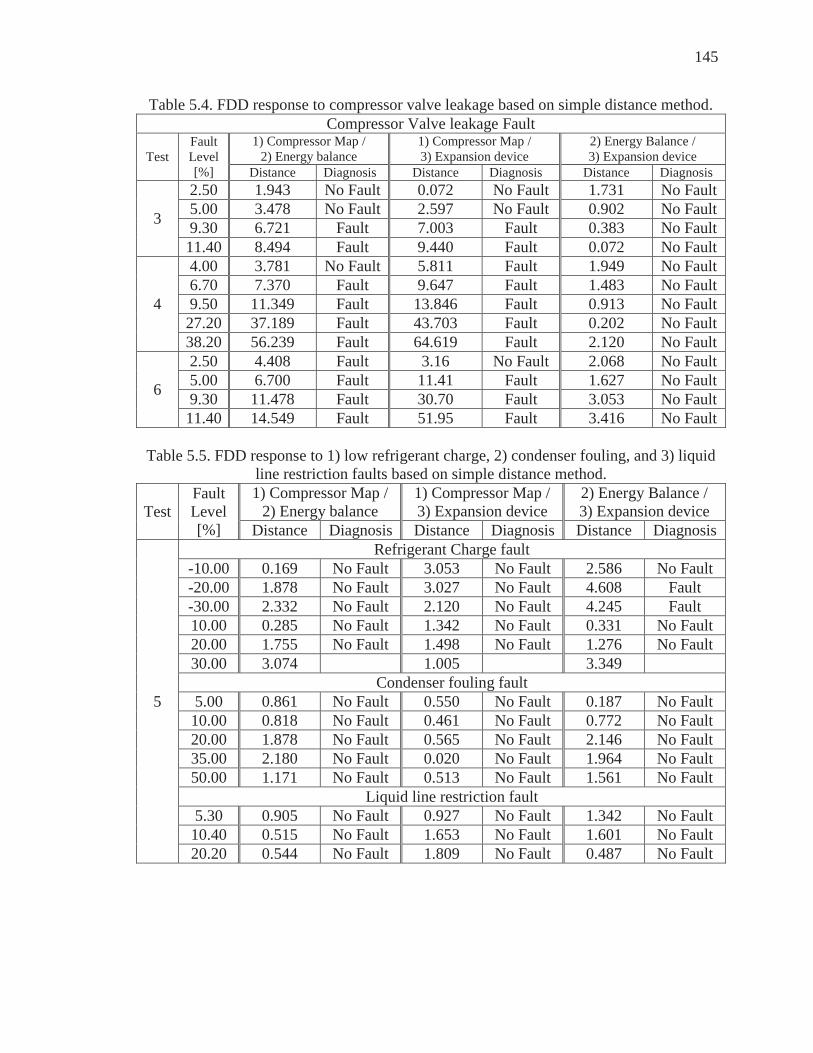
145

Table 5.4. FDD response to compressor valve leakage based on simple distance method. Compressor Valve leakage Fault





Distance Diagnosis Distance Diagnosis Distance Diagnosis

3

2.50 1.943 No Fault 0.072 No Fault 1.731 No Fault 5.00 3.478 No Fault 2.597 No Fault 0.902 No Fault 9.30 6.721 Fault 7.003 Fault 0.383 No Fault 11.40 8.494 Fault 9.440 Fault 0.072 No Fault

4

4.00 3.781 No Fault 5.811 Fault 1.949 No Fault 6.70 7.370 Fault 9.647 Fault 1.483 No Fault 9.50 11.349 Fault 13.846 Fault 0.913 No Fault 27.20 37.189 Fault 43.703 Fault 0.202 No Fault 38.20 56.239 Fault 64.619 Fault 2.120 No Fault

6

2.50 4.408 Fault 3.16 No Fault 2.068 No Fault 5.00 6.700 Fault 11.41 Fault 1.627 No Fault 9.30 11.478 Fault 30.70 Fault 3.053 No Fault 11.40 14.549 Fault 51.95 Fault 3.416 No Fault

Table 5.5. FDD response to 1) low refrigerant charge, 2) condenser fouling, and 3) liquid

line restriction faults based on simple distance method.





Distance Diagnosis Distance Diagnosis Distance Diagnosis

5

Refrigerant Charge fault -10.00 0.169 No Fault 3.053 No Fault 2.586 No Fault -20.00 1.878 No Fault 3.027 No Fault 4.608 Fault -30.00 2.332 No Fault 2.120 No Fault 4.245 Fault 10.00 0.285 No Fault 1.342 No Fault 0.331 No Fault 20.00 1.755 No Fault 1.498 No Fault 1.276 No Fault 30.00 3.074 1.005 3.349

Condenser fouling fault 5.00 0.861 No Fault 0.550 No Fault 0.187 No Fault 10.00 0.818 No Fault 0.461 No Fault 0.772 No Fault 20.00 1.878 No Fault 0.565 No Fault 2.146 No Fault 35.00 2.180 No Fault 0.020 No Fault 1.964 No Fault 50.00 1.171 No Fault 0.513 No Fault 1.561 No Fault

Liquid line restriction fault 5.30 0.905 No Fault 0.927 No Fault 1.342 No Fault 10.40 0.515 No Fault 1.653 No Fault 1.601 No Fault 20.20 0.544 No Fault 1.809 No Fault 0.487 No Fault

146

Figure 5.7 shows comparisons between predictions of the capacity virtual sensor

and the expected performance (capacity) for system E-3 under no fault and a compressor

valve leakage fault at different levels. The normalized capacity ratio is the percentage of

estimated capacity based on the expected performance map or virtual sensor with respect

to rated capacity. Four types of data points are presented: 1) no fault (Nofault); 2) faults

at a low level that don’t pass the threshold for fault detection (Comp. valve leak_nofault);

3) faults that pass the fault detection threshold but have less than a 10% impact on

capacity (Comp. valve leak_no service); and 4) faults that pass both the fault detection

and capacity impact thresholds and therefore might be considered for service (Comp.

valve leak_need service). The predicted and normal expected values match within about

3% under no-fault conditions. For compressor valve leakage with no fault detection, it

can be seen that there are no data points that are out of range of the 10% capacity

thresholds. For compressor valve leakage with fault detection, it can be seen that there are

three points (highlighted as needing service in the plot) that are outside of the thresholds

for capacity. For example, compressor valve leakage with a 20% fault level was

identified with a 25% capacity reduction compared to the reference value. The capacity

ratio decreases with increasing compressor valve leakage fault level because of the

reduction of refrigerant mass flow rate.

Figure 5.8 shows similar results for the outputs of the efficiency (COP) virtual

sensor plotted versus the expected performance (COP) for system E-3 under a

compressor valve leakage fault. The COP ratio is the ratio of the current equipment COP

to the normal expected performance. The COP ratio has the same trend as the capacity

147

ratio. Overall, the fault impact evaluation can be used for fault diagnosis in combination

with fault detection based on virtual sensors.

Figure 5.9 shows comparisons between capacity performance predictions of the

virtual sensors and the expected performance model for system E-3 under other system

faults. Though five data points were detected as condenser fouling or refrigerant charge

fault, the performance degradations were not enough to pass the capacity threshold. There

are seven data points with impacts greater than the capacity threshold. When the severity

of the fault levels increases, the performance ratio is decreased.

Figure 5.7. Comparison between the virtual sensors and the expected performance model

(Capacity) for system E-3 under compressor valve leakage fault.

148

Figure 5.8 Comparison between the virtual sensors and the expected performance model

(COP) for system E-3 under compressor valve leakage fault

Figure 5.9. Comparison between the virtual sensors and the expected performance model

for system E-3 under other faults conditions.

149

CHAPTER 6. FAULT DETECTION BASED ON VIRTUAL SENSORS FOR LABORATORY AND FIELD TESTS

A FDD method based on a number of virtual sensors that are useful for fault

detection and diagnoses were developed and evaluated. They were applied to an RTU in

the laboratory and field and to a direct expansion (DX) system at Building 101 in the

Navy Shipyard, Philadelphia. The diagnostic methods based on virtual sensors can

identify and isolate specific faults (e.g. low refrigerant charge and fouling) using a

number of surface-mounted temperature measurements. Fault impact models for decision

support were also developed and evaluated to estimate performance reduction due to fault

conditions. The field test for the DX system in Building 101 was performed to simulate

refrigerant charge faults and condenser fouling. VRC and VAF sensors were developed

and demonstrated for various charge levels and condenser blockages. A user interface of

a complete implementation and demonstration of an AFDD system applied to the RTU

system is described in this section. The implementation incorporates integrated virtual

sensors to provide diagnostic outputs and performance impacts of faults with low sensor

costs.

150

6.1 RTU FDD Assessments using Laboratory and Field Test Data

6.1.1 System Description and Test Conditions

RTU laboratory test data provided by the equipment manufacturer was used to

evaluate the performance of virtual sensors. In addition to laboratory testing, a field test

dataset that included transients associated with on/off cycling of the equipment and the

effects of solar, wind, and rain collected by the manufacturer were used to evaluate the

performance of virtual sensors.

System descriptions are given in Table 6.1 and testing conditions are listed in

Table 6.2. Table 6.1 gives specifications for a 7.5 ton RTU system where data were

obtained through laboratory testing, a 10 ton RTU system installed in the field, and a 4

ton RTU system that was tested in the psychrometric chambers at the Herrick

Laboratories. The three systems employed a TXV as the expansion device and R-410A as

the refrigerant.

Table 6.1. Specification of RTU system. RTU

system Nominal capacity Refrigerant Expansion

type Indoor airflow

Outdoor airflow

Total power

Indoor fan

Outdoor fan

[tons] - - [CFM] [CFM] [W] [W] [W] I 7.5

R410A TXV 2885 5750 6800 1350 497

II 10 3400 8300 9750 2760 800 III 4 1400 3800 3750 250 380

The ranges of test conditions are given in Table 6.2. The laboratory tests for RTU

system I were performed at different operating conditions. The indoor air flow rate

ranged from 60 to 100% of nominal. The ambient temperatures ranged between about 83

and 113 °F. Indoor dry/wet bulb temperatures were considered from 70 to 80 °F and from

60 to 66 °F, respectively. The outdoor air ventilation damper position was kept at 0%

outdoor air for all tests.

151

The field tests for RTU II were performed under different refrigerant charge and

condenser fouling conditions. The refrigerant charge was varied from 70 to 140% of

normal charge. Condenser fouling was simulated by blocking a portion of the condenser

heat exchange area. The effects of reduced air flow rate were considered from about 45 to

100% of the normal value. During the field test period, the outdoor-air temperature was

as high as 97 °F during the daytime and dropped as low as 61 °F. The indoor dry/wet

bulb temperatures were as high as 86/75 °F and dropped as low as 68/38 °F. The

outdoor-air damper openings were varied between 0 and 100% during each normal and

faulty test condition.

Laboratory tests were performed with the RTU system III with faults imposed.

Since an extra liquid line was added in order to install the refrigerant mass flow meter,

tests were performed to determine the nominal charging amount. The refrigerant charge

levels were determined using the subcooling obtained from the technical data provided

from the manufacturer. Refrigerant charge levels were varied between 50% and 100% of

nominal charge levels with outdoor temperatures between about 65 °F and 115 °F. Data

for relatively low outdoor temperatures were used to validate the algorithms for

conditions that would occur during the off season, when regular maintenance procedures

are often performed. Condenser fouling was simulated by blocking different amounts of

the air inlet area. The blocked heat exchanger area ranged from 0% to 70%. The

simulated method for evaporator fouling was to reduce the indoor fan speed.

152

Table 6.2. Testing conditions.

RTU

Return air Ambient Indoor Outdoor System

Dry temp.

Wet temp.

Dry temp.

Wet temp.

Airflow rate of

nominal

Block ratio

Damper opening

Refrigerant charge level

[°F] [°F] [°F] [°F] [%] [%] [%] [%]

I 71~81 60~66 83~113 - 60,78, 100 100 0 70, 75, 80, 85, 100, 140

II 68~86 38~75 46~66 82~97 100 45,57, 70,100

0,25,50, 75,100

70,75,80, 85,100,140

III 80 67 65~115 - 35, 50, 100 0, 15, 20, 45, 60, 70 0, 50 50, 60, 70,

85, 100

6.1.2 Virtual Sensor Developments and Evaluations

A number of virtual sensors (VRC, VRMF, VCP and VAF sensors) were

developed using the RTU test data. The accuracy of the virtual sensors was evaluated for

all of the test data in terms of the RMS deviation from the actual measurements presented

on a percentage basis. Overall virtual sensors showed good performance within 10% of

real measurements regardless of the different operating temperatures and faulty test

conditions. The outputs of virtual sensors can provide information regarding the presence

of certain faults and are relatively insensitive to the existence of other system faults.

6.1.2.1 VRC Sensor: Refrigerant Undercharge and Overcharge

VRC sensor model 3 based on tuned parameters was evaluated in terms of RMS

deviation between predicted and actual charge levels relative to nominal charges. Figures

6.1 and 6.2 show the performance of VRC sensor model 3 using tuned parameters for

RTU system I and system III. The parameters for the VRC sensors were tuned by using

ten data points under four different refrigerant levels for RTU system I and five data

points collected at the rated test condition over a range of refrigerant charge levels for

153

RTU system III. The VRC sensor can provide accurate estimates of refrigerant charge

level under a large variation of indoor and ambient conditions and different faulty

conditions. Overall, the VRC sensor provided charge predictions that were within 10% of

the actual charge and were typically within 5%. Based on the data analyzed in this study,

it appears that undercharging a unit by 10% would result in less than a 5% impact on

efficiency and overcharging by 10% would have a minimal impact. Therefore, a VRC

accuracy of 10% is acceptable.

Figure 6.1. Performance of VRC sensor model 3 based on tuned parameters for RTU I

laboratory data.

154

Figure 6.2. Performance of VRC sensor model 3 based on tuned parameters for the RTU

III laboratory data.

The existing charging method specified by the manufacturer was applied to RTU

II system and compared with the VRC sensor model 3 based on tuned parameters. The

existing charging approach requires compressor discharge pressure and liquid line

temperature measurements to verify refrigerant charge amount. The technician evaluates

whether to add or remove refrigerant based on a difference between the measurement and

a target value based on the charging chart supplied by the manufacturer. For each charge

level, simulated condenser fouling were introduced to the system to test its robustness.

Figure 6.3 and Figure 6.4 show the results of the existing field charging method

and VRC sensor for the RTU system II under the various operating conditions. The solid

line indicates the target pressure and temperature combination. The points that are above

the line indicate that more refrigerant needs to be added to the system and those below

the line indicate that refrigerant needs to be removed. Figure 6.3 shows the charging

155

results without heat exchanger blocking. It showed 70~80% as undercharged, 90~100%

as nominal, and 120% as overcharged.

Figure 6.4 shows the charging results when heat exchanger blockage is present.

While it showed 70% as undercharged, 80~90% was detected as nominal charge and

100~120% was detected as overcharged. This suggests that when there is condenser

fouling the charging method can indicate normal charge even when the unit is

undercharged by as much 20%. In addition, the manufacturers’ charge verification

utilizes pressure gauges or transducers installed at the service valve. The installation of

these gauges or transducers can lead to refrigerant leakage. Because of these limitations,

the current protocols for checking refrigerant charge may be doing more harm than good

in many situations.

Figure 6.3. Charging results based on manufacturers’ charging method for RTU II under

no heat exchanger blocking.

156

Figure 6.4. Charging results based on manufacturers’ charging method for RTU II under

heat exchanger blocking.

Figure 6.5 shows the accuracy of the VRC sensor model 3 based on tuned

parameters for RTU system II under conditions without fouling. The VRC sensor based

on tuned parameters showed RMS errors of 4 %. The VRC sensors work very well

under all refrigerant charge conditions. A relatively accurate prediction of refrigerant

charge amount was made even when refrigerant was overcharged at low ambient

temperature conditions. Overall, the manufacturers’ charging method and VRC sensor

can provide accurate estimates when no heat exchanger blocking is present.

Figure 6.6 shows the results of VRC sensor model 3 for RTU system II based on

tuned parameters with heat exchanger blocking. VRC model 3 shows good performance

for predicting refrigerant charge levels when condenser fouling conditions exist. Some

errors between 80 and 90% refrigerant charge levels were slightly over 10%. These

points are associated with large condenser blocking of approximately 50%. The cases

where the VRC sensor had difficulty were when the system operated with zero

157

subcooling at over 50% reduction of condenser air flow rate. In this case, the VAF

sensor for the condenser would be helpful at predicting the condenser fouling fault.

Overall, the VRC sensor provides accurate refrigerant charge estimates regardless of the

condenser fouling.

Figure 6.5. Performance of VRC sensor model III based on tuned parameters for RTU II

under no condenser fouling.

Figure 6.6. Performance of VRC sensor model III based on tuned parameters for RTU II

under condenser fouling.

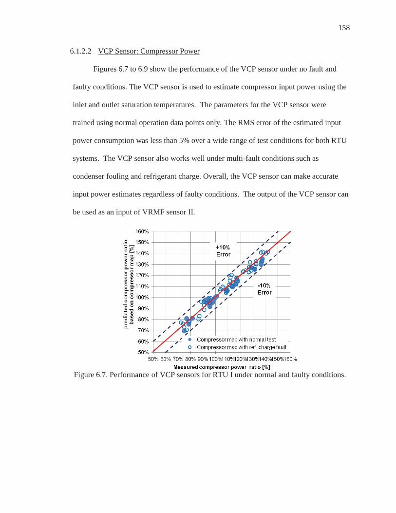
158

6.1.2.2 VCP Sensor: Compressor Power

Figures 6.7 to 6.9 show the performance of the VCP sensor under no fault and

faulty conditions. The VCP sensor is used to estimate compressor input power using the

inlet and outlet saturation temperatures. The parameters for the VCP sensor were

trained using normal operation data points only. The RMS error of the estimated input

power consumption was less than 5% over a wide range of test conditions for both RTU

systems. The VCP sensor also works well under multi-fault conditions such as

condenser fouling and refrigerant charge. Overall, the VCP sensor can make accurate

input power estimates regardless of faulty conditions. The output of the VCP sensor can

be used as an input of VRMF sensor II.

Figure 6.7. Performance of VCP sensors for RTU I under normal and faulty conditions.

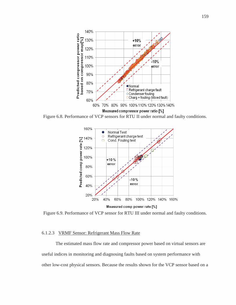
159

Figure 6.8. Performance of VCP sensors for RTU II under normal and faulty conditions.

Figure 6.9. Performance of VCP sensor for RTU III under normal and faulty conditions.

6.1.2.3 VRMF Sensor: Refrigerant Mass Flow Rate

The estimated mass flow rate and compressor power based on virtual sensors are

useful indices in monitoring and diagnosing faults based on system performance with

other low-cost physical sensors. Because the results shown for the VCP sensor based on a

160

compressor map are consistent with the power measurement, the predictions of VRMF

sensor based on energy balance were reliable.

Figures 6.10 to 6.12 show comparisons of VRMF sensor I predictions (based on a

compressor map) and sensor II outputs using an energy balance under no-fault and faulty

conditions. The RMS errors between VRMF models I and II were less than 10% for

single faults such as evaporator fouling, condenser fouling and refrigerant charge. The

errors are somewhat higher (9%) at high refrigerant charge level and low evaporator

fouling, but the sensor outputs are still reasonable for this fault. The VRMF sensors also

work well with multiple simultaneous fault conditions for most cases. However, for

some combinations of refrigerant charge and fouling that were tested, the RMS errors

between VRMF sensor I and II were over 10%. The larger errors occurred when the

superheat at the compressor inlet was below 1.5 °F. The incorrect compressor suction

enthalpy due to a two-phase refrigerant inlet state led to the inaccurate estimations. The

system was overcharged and serious evaporator fouling was applied in these situations.

161

Figure 6.10. Performance of VRMF sensor for RTU I based on model I and II under

normal and faulty conditions.

Figure 6.11. Performance of VRMF sensors for RTU II based on model I and II under


162

Figure 6.12. Performance of VRMF sensors for RTU III based on model I and II under


Figures 6.13 to 6.15 show comparisons of VRMF sensor II predictions based on

the energy balance method and VRMF sensor III outputs using the TXV model both

with and without faults. The RMS errors for models I and III are less than 10% and the

sensors work well regardless of the fault conditions applied. Some of the larger errors

may be associated with two-phase refrigerant conditions at the TXV inlet with near-zero

subcooling under low refrigerant charge and condenser fouling conditions.

163

Figure 6.13. Performance of VRMF sensor for RTU I based on model II and III under


Figure 6.14. Performance of VRMF sensor for RTU II based on model II and III under


164

Figure 6.15. Performance of VRMF sensor for RTU III based on model II and III under


6.1.2.4 VAF Sensor: Improper Outdoor Air Flow Rate

The VAF sensor for the condenser based on an energy balance was evaluated for

the RTU II test data. Figures 6.16 and 6.17 show the condenser air flow rate estimated

with the VAF sensor for the RTU systems with normal and single faulty conditions.

Predicted air flow rates based on the VAF sensor can be compared to a target air flow

rate to detect fouling. The target flow can be obtained from a manufacturer’s catalog or

from a normal value when the FDD scheme is implemented assuming that there is no

fouling.

Figure 6.16 shows the results of the VAF sensor under 100% refrigerant charge.

The VAF sensor predicted the target condenser air flow rate within 15% except under

condenser fouling fault conditions. When the blocking level was over 40%, the air flow

rate decreased to 65% of the nominal air flow rate. Figure 6.17 shows similar results but

165

with a larger spread of predictions when the system was undercharged. As the severity

of the condenser fouling increases, the estimated air flow rate is decreased. The results

also show that the condenser fouling fault is decoupled from refrigerant charge faults.

Figure 6.16. Performance of VAF sensor (condenser) for RTU II under normal refrigerant

charge.

Figure 6.17. Performance of VAF sensor (condenser) for RTU II under different

refrigerant charge levels.

166

6.1.2.5 VAF Sensor: Improper Indoor Air Flow Rate

Figure 6.18 shows the accuracy of the air flow predictions from an energy balance

for RTU III system with normal and faulty refrigerant charge. The indoor unit typically

has more than one speed setting, but the air flow is constant for a given setting. Therefore,

the VAF sensor can be used to estimate the air flow rate for each fan setting. These

estimates can then be compared with a target air flow rate. The VAF sensor for the

evaporator predicted the target air flow rate based on the fan setting within 10%. The

VAF sensor based on an energy balance model has the limitation of not being valid when

subcooling at the outlet of the condenser is zero. However, zero subcooling is typically

associated with low refrigerant charge, which can be diagnosed using the VRC sensor.

Figure 6.18. Predicted evaporator air flow from an energy balance versus expected value

based on fan setting for RTU III.

167

6.1.3 Diagnostics Performance Evaluations

6.1.3.1 Diagnostics Performance Evaluation for RTU I

To evaluate the impact of faults on performance, capacity and COP ratio were

calculated and compared to rated reference values. The impacts of the various faults were

used in deciding thresholds for the FDD demonstration system. Information about

capacity, power consumption, and energy efficiency can be used in real-time monitoring

of the economic status of the equipment and for decision support.

Figure 6.19 shows comparisons between the normal expected performance model

and virtual sensors for energy efficiency under no-fault test conditions. The energy

efficiency ratio was calculated as the ratio of estimated energy efficiency based on virtual

sensors or the expected value from a performance map divided by the rated value

provided by product specifications. The expected performance model matched the virtual

sensor performance very well. This means that the expected performance model can be

used to estimate normal energy efficiency at faulty conditions.

Figure 6.20 shows comparisons between the expected performance model and the

virtual sensor under different operating conditions and refrigerant charge levels. When

the VRC sensor detects 75% as the charge level with fault detection, it can be seen that

all data points are lower than the threshold for energy efficiency. This means the potential

energy savings after service is small while service costs would be relatively high. When

the refrigerant charge level is 70%, the current energy efficiency ratios were reduced

outside the range of the thresholds. Overall, the service for the RTU system might be

justfified when the VRC sensor indicates 70% refrigerant charge level.

168

Figure 6.19. Comparison between the virtual sensor and the expected performance model

for RTU system I under normal conditions.


for RTU system I under refrigerant undercharge fault conditions.

169

6.1.3.2 Diagnostics Performance Evaluation for RTU II

Figure 6.21 shows a comparison between the virtual sensor and the expected

model under condenser fouling fault conditions. The energy efficiency degradation is

lower than the threshold which indicates that the fault impact for condenser fouling is not

sufficiently severe to require service. The energy efficiency ratio decreases with

increasing condenser fault levels. Although the VAF sensor indicates 40% air flow

reduction, the energy efficiency was only degraded by about 7 ~ 9%.

Figure 6.22 shows comparisons between the virtual sensor and the expected

model under the combination of 90% refrigerant charge and various condenser fouling

conditions. When blocked heat exchanger areas were 43 and 53%, indicating condenser

fouling based on the VAF sensor, it would result in over 10% energy efficiency

degradation. For a 30% condenser fault level, the energy efficiency degradation was less

than 10%.

Figure 6.23 shows comparisons between the virtual sensor and the expected

model under the combination of 80% refrigerant charge and various condenser fouling

conditions. It can be seen that energy efficiency degrades between about 10~20% for all

condenser fouling levels considered. When an 80% refrigerant charge fault occurred with

no blocked area, the average energy penalty was about 8%.

Figure 6.24 shows comparisons between virtual sensor and expected model

outputs under the combination of 70% refrigerant charge and various condenser fouling

conditions. Overall, service for the RTU system might be warranted when the VRC

sensor indicates 70% refrigerant charge level or less.

170

Figure 6.21. Comparison between the virtual sensor and the expected performance model for RTU system II under condenser fouling fault conditions.

Figure 6.22. Comparison between thevirtual sensor and the expected performance model for RTU system II under 90% refrigerant charge and condenser fouling fault conditions.

171

Figure 6.23. Comparison between the virtual sensor and the expected performance model for RTU system II under 80% refrigerant charge and condenser fouling fault conditions.

Figure 6.24. Comparison between the virtual sensor and the expected performance model for RTU system II under 70% refrigerant charge and condenser fouling fault conditions.

6.1.3.3 Diagnostics Performance Evaluation for RTU III


performance model under no-fault conditions. The expected model and virtual sensor

outputs agree well regardless of operating conditions for normal operation.

172


performance model under different refrigerant charge conditions. When the refrigerant

charge level is in the range of 75% to 100%, the performance degradation is not

sufficiently severe to require service for a refrigerant charge fault. The RTU system is

still able to provide adequate energy efficiency with a 25% undercharge condition. When

the refrigerant charge amount is below this range, there are larger differences between the

predicted and expected values. The energy efficiency degradation is up to 20 ~ 40%,

which is coincident with the low refrigerant charge fault indicated by the VRC sensor.

Overall, the RTU system that is charged 35% lower than nominal charge can experience

a 15% average efficiency degradation.


for RTU system III under no faults conditions.

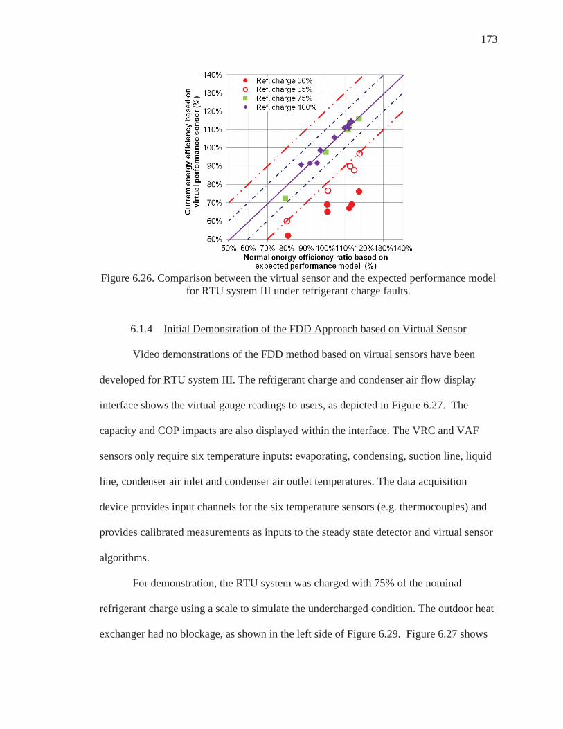
173


for RTU system III under refrigerant charge faults.

6.1.4 Initial Demonstration of the FDD Approach based on Virtual Sensor

Video demonstrations of the FDD method based on virtual sensors have been

developed for RTU system III. The refrigerant charge and condenser air flow display

interface shows the virtual gauge readings to users, as depicted in Figure 6.27. The

capacity and COP impacts are also displayed within the interface. The VRC and VAF

sensors only require six temperature inputs: evaporating, condensing, suction line, liquid

line, condenser air inlet and condenser air outlet temperatures. The data acquisition

device provides input channels for the six temperature sensors (e.g. thermocouples) and

provides calibrated measurements as inputs to the steady state detector and virtual sensor

algorithms.

For demonstration, the RTU system was charged with 75% of the nominal

refrigerant charge using a scale to simulate the undercharged condition. The outdoor heat

exchanger had no blockage, as shown in the left side of Figure 6.29. Figure 6.27 shows

174

that the gauge readings displayed within the user interface correctly indicate a 75%

refrigerant charge level and 100% condenser air flow rate (0% condenser fouling). The

capacity and COP ratio displays indicate 95% and 96% of normal performance for the

current operation. The results demonstrate that the impact of refrigerant charge on

performance is relatively small for 75 % of the rated charge at this operating condition.

However, there was a dramatic reduction in both cooling capacity and energy efficiency

when charge was decreased below 70% refrigerant charge, as shown in chapter 2.

The system was recharged to 100% of the nominal charge level by weighing the

change in mass of a refrigerant canister. For this situation, Figure 6.28 shows that the

VRC and VAF sensor gauges indicated 100%, respectively. Both capacity and COP ratio

were increased to 98 % of the expected values.


level demonstration.

175



Condenser fouling was simulated by blocking the bottom part of the heat

exchanger with paper strips. Figure 6.29 shows an example of simulated condenser

fouling with a fault level of 50% (shown on the right side). The fault level is defined as

the percentage of blocked heat exchanger face area. For 70% blockage, Figure 6.30

shows that the VAF sensor indicated a condenser air flow rate that was 63% of the

normal value. A condenser fouling fault could be detected by comparing this estimated

air flow rate with a target value. As the severity of the condenser fouling increases, the

estimated air flow rate decreases relative to the target value. The VRC sensor made

accurate predictions of the refrigerant charge amount even when the outdoor heat

exchanger was blocked.

176

Figure 6.29. Condenser status of RTU system (left side: normal & right side: 50%

blocking).



6.2 DX Systems Field Testing

6.2.1 Field Fault Test Conditions and System Descriptions

In addition to developing the RTU demonstration, virtual sensors for DX systems

at Building 101 at the Navy Shipyard in Philadelphia, PA have been developed based on

historical data. Refrigerant charge and condenser fouling diagnostics were demonstrated

based on virtual sensors for the condensing units associated with the DX systems. Table

6.3 shows the system specifications for DX systems 2 and 3 at Building 101. R-22 was

177

used as the refrigerant and two semi-hermetic compressors with 3 stages each and a TXV

as the expansion device were employed. The systems have two separate circuits which

are connected to a separate condenser and compressor. The refrigerant charge and

condenser fouling diagnostics are demonstrated using these DX systems.

Table 6.3. System specifications of DX systems 2 & 3. Rated

Capacity Refrigerant Expansion Type

Compressor Type

Outdoor coil airflow rate

Total power

Outdoor fan Power

[Mbtu] - - - [CFM] [kW] [kW] 738 R22 TXV Semi-Hermetic 36800 64.1 6.0 (4 fan)

6.2.2 Virtual Sensor Development and Evaluation

6.2.2.1 VRC Sensor Development and Evaluation

Historical data for DX systems in Building 101 were obtained from continuous

monitoring. Virtual sensors based on this data are developed and evaluated in this section.

Virtual sensors can be embedded in a permanently installed control or monitoring system

for DX systems and used by the FDD algorithms to identify specific faults and handle

simultaneous faults.

First, a VRC sensor was developed for the DX systems using data filtered by a

steady state detector. Measured data for the condensing unit of DX system 3 in Building

101 were used to evaluate the robustness of the VRC sensor. Figure 6.31 shows the

sample outputs of the VRC sensor based on the use of default parameters for DX system

3 for circuits A & B. The outdoor temperature during this period ranged between 86 and

93 °F. Under this range of outdoor temperatures, the VRC sensor gave charge level

predictions that varied by less than 10%. DX system 3 shows relatively larger deviations

178

and it is due to the fact that the fans and compressor are loading and unloading. These

results are typical of the variations encountered during the test period in May.

Figure 6.31. VRC sensor outputs based on default parameters for DX unit 3 circuits A &

B.

The VRC sensor was also applied to steady-state summer data to evaluate its

consistency in predicting normal charge levels over a wide range of operating conditions.

Figure 6.32 shows outputs from the VRC sensor based on default parameters for DX

system 3 circuits A & B for operating conditions during the summer where steady-state

conditions were detected. The outdoor temperature during this period was between 70

and 100 °F. Under this range of outdoor temperatures, the VRC sensor gave charge level

predictions that varied by less than 7% regardless of the time and cloud cover conditions.

The next section shows the performance of the VRC sensor for DX system 3 under

different charge levels and over a wider range of operating conditions.

179

Figure 6.32. VRC sensor outputs based on default parameters for DX unit 3 circuits A &

B.

6.2.2.2 VRMF Sensor Development and Evaluation

For monitoring the health status of the DX system, the outputs of the VRMF

sensor were used to estimate system performance and energy efficiency with low-cost

physical sensors. Figure 6.33 shows outputs from a VRMF sensor developed for DX

system 2 circuit A. The mass flow rate predictions were determined from a compressor

energy balance using heat loss estimates and predictions of VCP sensor. The predicted

refrigerant mass flow rates could not be compared with actual measurements due to an

absence of refrigerant mass flow meter data. The refrigerant mass flow rate was estimated

to be 100% when three compressors were used and 60% when two compressors were

used. The rated refrigerant mass flow rate was determined as estimated mass flow rate

under three stages of compressor. The results for the VRMF sensor are presented as the

ratio of the estimated flow rate to the rated refrigerant mass flow rate at the measured

operating conditions. Although it is not possible to validate the predictions, the results

180

clearly show the overall dependence on compressor staging. These estimations are used

as inputs for other fault detection (e.g. condenser fouling).

Figure 6.33. VRMF sensor outputs based on an energy balance for DX unit 2 circuit A.

Although refrigerant flow measurements were not available, VRMF sensor I,

based on compressor maps obtained from the manufacturer, was used in order to assess

VRMF sensor II based on an energy balance. In order to assess the accuracy of the

maps, the predicted power from the compressor map was compared to power

measurements and the results were within 10% regardless of the number of compressor

stages operating, as shown in Figure 6.34. Figure 6.34 also shows comparisons of the

map-based flow estimates and outputs from the VRMF sensor for DX system 3. For

these plots, the compressor power and mass flow rate are referenced to rated values for

the compressor. The data were obtained from summer months and filtered for steady-

state operation.

181

Figure 6.34. Accuracy of predicted power based on compressor map for DX system 3 circuits A & B.

6.2.2.3 VAF Sensor Development and Evaluation

Figure 6.35 shows outputs from a condenser VAF sensor for DX system 2

referenced to the expected flow rate for a single-fan operation. Again, there were no

direct measurements to validate the VAF sensor outputs, but the results show the

dependence on fan staging.

Figure 6.35. Performance of VAF sensors based on an energy balance for DX system 3.

182

6.2.2.4 Initial Demonstration of Virtual Sensors for DX Systems

Figure 6.36 shows the performance of the VRC, VRMF, and VAF sensors for the

DX system. The steady state detector using superheat filtered out the transient data,

which shows large deviations from predictions. When the steady state detector indicates

steady-state status, the three virtual sensors consistently estimate 100% of the expected

values.

Figure 6.36. Performance of the VRC, VRMF, and VAF sensors for the DX

system.

The user interface for diagnostic implementation has been developed for

demonstration with the DX system. The implementation incorporates integrated virtual

sensors to provide the diagnostic outputs and the performance impact of the fault(s) with

low sensor costs. The user interface includes 1) the status of the compressors and fans, 2)

VRC, VRMF and VRMF sensors, 3) performance indices for a DX system at Building

101 that show the impact of the fault(s) on overall performance (capacity and COP).

Figure 6.37 shows an example of the demonstration under 100% refrigerant charge level,

100% refrigerant mass flow rate and 0% condenser fouling.

183

Figure 6.37. Example of the virtual sensor display from a demonstration of the FDD tool

for the DX system.

6.2.3 Demonstration of the VRC and VAF sensors for the DX system

The demonstration of the FDD system based on virtual sensors for DX system 3

circuit A was performed under imposed refrigerant charge faults and condenser fouling.

The VRC sensor and the VAF sensor for the condenser were developed and demonstrated

for various charge levels and condenser blockages. The outputs of the virtual sensors can

provide information regarding the presence of a fault.

6.2.3.1 Refrigerant undercharge and overcharge for DX system 3 circuit A

Figure 6.38 shows the refrigerant charge test conditions for DX system 3 circuit A

along with an indicated of the range of subcooling (SC) associated with different charge

levels. The refrigerant charge level ranged from 50 to 130% in comparison with the rated

charge during testing that occurred in the summer of 2013. The charge level in August

2012 was used to define the “normal” system charge. Although it cannot be confirmed

that the August 2012 charge level was correct, the VRC sensor indicated a relatively

constant refrigerant charge amount during one year. The refrigerant charge fault was

simulated by adding more or less refrigerant to the system. For the overcharge condition,

184

the refrigerant was added from an R-22 refrigerant tank using a manifold gauge. The tank

was weighed using a digital scale. For the undercharge condition, refrigerant was

recovered from the system to an evacuated tank connected to the manifold gauge. The

recovered refrigerant amounts were also weighed using a digital scale.

Figure 6.38. Refrigerant charge test condition for DX system 3 circuit A.

Figure 6.39 shows the results of VRC sensors I and Ш based on tuned parameters

under conditions without condenser fouling. To increase the accuracy of the charge

determination, the parameters of the VRC sensor were tuned for the DX system using

measurements obtained at different refrigerant charge levels. The performance of VRC

sensors I and Ш is good since the actual and predicted charge levels match within about

10%. The VRC sensor was also found to be relatively insensitive to operating conditions

when the parameters were tuned with different refrigerant charge data. VRC models I and

III gave similar and accurate charge predictions.

185

Figure 6.40 shows the performance of VRC sensors I and Ш based on tuned

parameters under different condenser fouling conditions. There are relatively large errors

in refrigerant charge detection under condenser fouling conditions. As the refrigerant

charge level increases, there is a bigger difference between the predicted and real charge

amounts. This is because the subcooling at the condenser outlet is decreased with

increasing condenser fault levels due to the reduction in air-side heat transfer area. Also,

the performance of VRC sensor Ш is poor because there were cases of low subcooling.


parameters based on refrigerant charge test data).

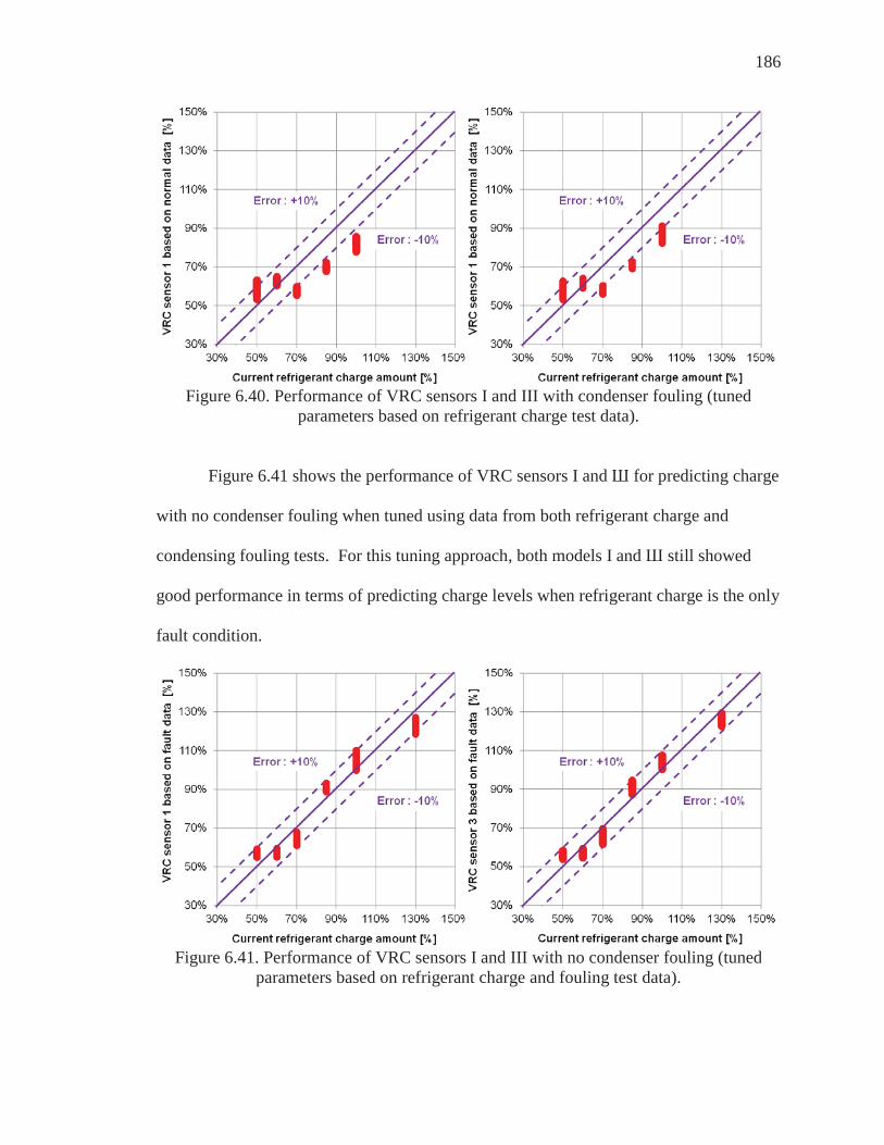
186


parameters based on refrigerant charge test data).

Figure 6.41 shows the performance of VRC sensors I and Ш for predicting charge

with no condenser fouling when tuned using data from both refrigerant charge and

condensing fouling tests. For this tuning approach, both models I and Ш still showed

good performance in terms of predicting charge levels when refrigerant charge is the only

fault condition.


parameters based on refrigerant charge and fouling test data).

187

Figure 6.42 shows the performance of VRC sensors I and Ш for predicting charge

level with condenser fouling when tuned using data from both refrigerant charge and

condensing fouling tests.. When VRC sensor I was applied with a fouled condenser, there

was no improvement compared to using the tuned parameters based on refrigerant charge

data only. However, Model III showed very significant improvement in cases where

model I did not work well. VRC sensor III gave charge level predictions that were within

10% of the actual charge regardless of the condenser fouling. Overall, VRC sensor

model Ш with tuned parameters based on all test data is relatively insensitive to the

existence of condenser fouling faults.


parameters based on refrigerant charge and fouling test data).

6.2.3.2 Improper Condenser Air Flow Rate for DX System 3 Circuit A

DX systems in Building 101 are located in areas surrounded by overgrown weeds

or fallen leaves. The outdoor heat exchanger may be easily contaminated by debris and

dust. The outdoor air flow degradation can also be caused by a defective fan motor. To

188

simulate condenser fouling or a defective fan motor fault for the DX system, the bottom

part of the heat exchanger area was blocked by several layers of paper towels. Figure

6.43 shows the condenser with 25% and 37.5% face area blockage or fault levels of 25%

and 37.5%, respectively. The blocked heat exchanger area ratio is defined as the ratio of

blocked face area with paper divided by the total face area of the heat exchanger.

Figure 6.43. Condenser with lower face area blockage ( 25% (Left) and 37.5% (Right) of the entire finned area blocked ).

Figure 6.44 shows the output of the VAF sensor for the condenser under different

refrigerant charge conditions. A condenser fouling fault can be detected by comparing the

estimated air flow rate with a rated value provided by the system specifications. The left

graph in Figure 6.44 shows the output of the VAF sensor under 50% refrigerant charge

conditions. The percentage of air flow rate was calculated by the ratio of predicted air

flow rate divided by rated air flow rate. During the field test period, the outdoor

temperature was as high as 38 °C during the daytime and dropped as low as 15 °C. Under

this range of outdoor temperatures, the VAF sensor gave air flow rate predictions that

189

were within 10% of the rated value regardless of the time and cloud cover conditions. As

the severity of the condenser fouling increases, the estimated air flow rate is decreased.

For condenser fouling fault conditions, the difference between the predicted air

flow rate and its expected value was within 10%, indicating acceptable accuracy of the

VAF sensor. When the condenser blockage levels were 20% and 37.5%, the estimated

air flow rate from the VAF sensor decreased by 15% and 20% in comparison with target

value.

The right graph in Figure 6.44 shows the output of the VAF sensor under 70%

refrigerant charge fault conditions. The VAF sensor predicted the target condenser air

flow rate within 10% under un-fouled conditions. For 20% and 37.5% condenser

blockage ratios, the output of the VAF sensor indicated 13% and 20% air flow rate

reductions, which is similar to the result with 50% refrigerant charge. The reduction of

condenser air flow rate is proportional to the fault level and is independent of refrigerant

charge level. Overall, the outputs of the VAF sensor show that the condenser fouling

fault is decoupled from refrigerant charge faults.

Figure 6.44. Performance of the VAF sensor for the DX system under 50% and 70%

refrigerant charge faults.

190

6.3 Embedded Automated Fault Detection and Diagnostic (AFDD) System

This section presents the interface for a complete implementation and

demonstration of an AFDD system applied to RTU II field test data. The implementation

incorporates integrated virtual sensors to provide the diagnostic outputs and the

performance impact of the fault(s). The AFDD RTU demonstration system provides the

following diagnostic outputs: 1) loss of compressor performance, 2) low or high

refrigerant charge, 3) fouled condenser or evaporator filter, 4) faulty expansion device or

liquid-line restriction, and 5) economizer faults. Health and economic status reports for

equipment can be generated using fault impact indices, such as system cooling capacity

and efficiency (COP). In particular, the fault impact indices can be used to assess the

economics associated with servicing a unit if faults exist.

6.3.1 User Interface Development

The Automated FDD system incorporates 1) the status of compressors and fans

and the steady state detector, 2) the component fault identification information based on

integrated virtual sensors, 3) health and economic status based on performance indices

for on-line monitoring and 4) the complete diagnostic information about FDD status to

choose proper action, shown in Figure 6.45.

The status of fans and compressors is displayed on the left side. If steady-state

conditions are detected, shown on the middle of the left side, the virtual sensors will

indicate their detected values. Virtual sensors were implemented for the compressor,

expansion device/liquid line restriction, condenser and evaporator fouling, refrigerant

191

charge and economizer. The output of a virtual sensor can be compared to the output of a

real sensor or other virtual sensors in order to detect and localize a fault within the system.

On the right side, the system performance is also displayed to show the capacity

and COP ratios. The capacity and COP ratios are the ratios of current equipment

performance from virtual sensors to that of the normal expected performance model. The

normal expected performance model was developed based on normal test data obtained

from the manufacturer. If faults exist, the capacity and COP ratios can be used to

determine whether the fault is severe enough to request service.

Figure 6.45. Implementation and demonstration of an automated FDD system for RTU

under normal conditions.

6.3.2 Virtual Sensor Implementation

Figure 6.46 shows refrigerant charge information that is displayed by clicking the

VRC sensor button. The user interface shows the current estimated level and other

statistical information. It also shows the data trends as time passes. In addition,

probability distributions are shown corresponding to the current estimations (red line) and

expected values for normal conditions (white line). The mean and standard deviation for

192

the current distribution is also presented in the user interface. The confidence interval is

used to indicate the reliability of the current charge level from the virtual sensor. The

difference between the current charge level and the expected value is used as a residual

input to a Bayesian classifier in order to evaluate whether a refrigerant fault is present.

The probability graph shows much larger differences between current and

expected probability distributions, indicating low a refrigerant charge fault. The trending

graph provides more evidence for the existence of this fault. The current and recent

trending of refrigerant charge levels is shown. In addition, probability distributions are

shown that correspond to the current estimations from the VRC sensor and the expected

values for a normal condition. The mean and standard deviation for the current

distribution is also presented. The difference between current and expected values is used

as a residual input to a Bayesian classifier in order to evaluate whether a refrigerant fault

is present. For the no-fault test data, there is a significant overlap between the current and

expected probability distributions indicating normal operation.

Figure 6.46. Implementation and demonstration of the VRC sensor under normal conditions.

193

Figure 6.47 shows the refrigerant mass flow rate information displayed on the

user interface. When the compressor fault button is selected, detailed refrigerant mass

flow rate information is obtained. Three VRMF sensors are implemented in the AFDD

system for the RTU. The virtual sensors use a compressor map and a TXV model as

current predictions and an energy balance as a normal expected prediction. Outputs from

the three VRMF sensors can be compared in order to detect a fault. The Bayesian

classifier is applied to each combination of residuals between two predictions to identify

the existence of a fault such as a compressor valve leakage or a faulty expansion device.

For the no-fault test data, there is a significant overlap between the current and expected

probability distributions, indicating normal operation. The capacity and COP ratios are

97% and 99% of the normal condition based on the expected performance model for

Figures 6.46 and 6.47. Based on the readings, the diagnostic outputs indicate at the

bottom right corner that the status of the RTU system is acceptable and any service is

unnecessary.

Figure 6.47. Implementation and demonstration of the VRMF sensor under normal

conditions.

194

Figure 6.48 shows the diagnostic interface based on the simulated fouling test data

with 65% condenser blocking. This interface appears when the condenser fault button is

selected. The condenser fouling fault can be detected by comparing the estimated air flow

rate with a target value. A VAF sensor indicates the condenser air flow rate as 50% of the

normal value. The probability graph shows much larger differences between current and

expected probability distributions, indicating the low air flow rate fault. It is also a good

feature for diagnosing fan problems.

Figure 6.48. Implementation and demonstration of the VRMF sensor under 50%

condenser blocking condition.

Figure 6.49 shows detailed refrigerant charge information based on the results with

85% refrigerant undercharge. This interface is obtained by clicking the VRC sensor

button. The probability graph shows large differences between the current estimated

refrigerant charge and the expected values. The trending graph provides more evidence

for the existence of this fault. Overall, the demonstration AFDD system recommends that

service is needed for this refrigerant undercharge fault. For this case, the capacity and

COP ratio were reduced to 72% and 74%, respectively, due to low charge and condenser

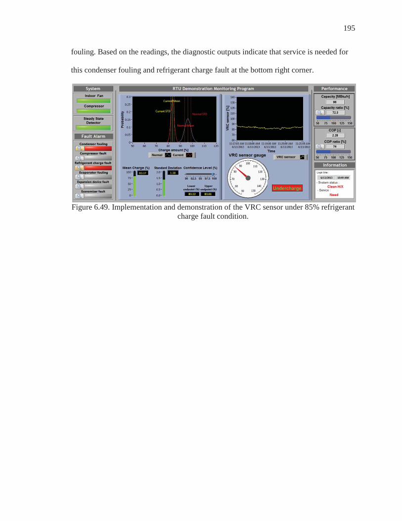
195

fouling. Based on the readings, the diagnostic outputs indicate that service is needed for

this condenser fouling and refrigerant charge fault at the bottom right corner.

Figure 6.49. Implementation and demonstration of the VRC sensor under 85% refrigerant

charge fault condition.

196

CHAPTER 7. COMPLETE EVALUATION, IMPLEMENTATION, AND VALIDATION OF RTU DIAGNOSTIC PERFORMANCE

Fault detection and diagnostic approaches described in the previous chapters are

validated using laboratory and field tests. This section describes a complete

implementation and demonstration of an FDD system applied to an RTU air conditioner

that incorporates integrated virtual sensors and fault impact evaluation.

The decoupling FDD system based on virtual sensors can be significantly more

sensitive to system malfunctions and easier to implement than the previous statistical

rule-based FDD method. The residuals between the output of virtual sensors and the

expected values representative of normal operation could be used to detect faults based

on Bayesian error classifiers, which estimate the overlap area between current and normal

probability distributions. In selecting the optimal thresholds based on no-fault data, there

is a tradeoff between sensitivity and false alarms. The fault diagnostic methods based on

virtual sensors are combined with fault detection and no separate diagnostic classification

is necessary.

Using existing normal performance test data, normal expected performance

models for capacity and power consumption were developed for the RTU system. These

models were used to quantify the performance reduction ratio between current equipment

performance measured by virtual sensors and normal expected performance. The fault

impact model was developed to determine whether a current fault, when detected, is

197

severe enough to request service. The model utilizes calculated performance reduction

ratios with a second-order function of the fault levels estimated by the virtual sensors.

7.1 System Specification

Table 7.1 shows the specifications of the 4 ton RTU system which was used for

FDD demonstration during laboratory tests. The system was modified to implement

faulty conditions based on the RTU system III used in chapter 6. Figure 7.1 shows a

diagram of the system that was investigated in the laboratory tests for RTU

demonstration. Various virtual sensors were implemented for the compressor, EEV as

expansion valve, condenser and evaporator heat exchangers, refrigerant charge, and

refrigerant filter/dryer in order to provide the following diagnostic outputs: 1) loss of

compressor performance, 2) low or high refrigerant charge, 3) fouled condenser or

evaporator filter, 4) faulty expansion device and 5) liquid-line restriction. In addition, the

demonstration implementation included an output of the impact of the fault(s) on overall

performance (COP).

Table 7.1. Specifications of the RTU system. RTU

System Nominal Capacity Refrigerant Expansion

Type Indoor airflow

Outdoor airflow

Total Power

Indoor fan

Outdoor fan

[tons] - - [CFM] [CFM] [W] [W] [W] IV 10 R410A EEV 1400 3800 3750 250 380

The condensing and evaporating pressure sensors are sensor-level virtual sensors

that are used as inputs for other virtual sensors. The refrigerant mass flow rate, air flow

rate and compressor power consumption are component-level virtual sensors used to

isolate component faults or as inputs to system-level virtual sensors. The performance

198

(capacity and energy efficiency) and refrigerant charge sensors are system-level virtual

sensors.

A compressor valve leakage fault was simulated using two hot gas bypass valves

which connect the compressor discharge line to the suction line, shown in number 1 of

Figure 7.1. For no-fault tests, the EEVs on the hot gas bypass line with zero opening

ensured no refrigerant flow through the valves. For compressor valve leakage faults, EEV

openings were controlled based on the target refrigerant mass flow rate.

Figure 7.1. RTU system diagram for demonstration in the laboratory.

An improper outdoor air flow rate was implemented by blocking the heat

exchanger with paper strips. An improper indoor air flow rate was simulated using

reduction of the external fan speed. A liquid line restriction fault or faulty expansion

valve was implemented by modulating a solenoid valve and EEV shown in Figure 7.1

number 4. For no-fault tests, the solenoid valve and EEV are fully opened to ensure a

199

normal liquid line pressure drop. Faulty conditions were simulated by increasing the

pressure drop based on the EEV opening and by modulating the solenoid valve between

open and closed positions. A refrigerant charge fault was simulated by reducing or

increasing the total amount of refrigerant charge.

7.2 Test Conditions

Laboratory tests were performed in the psychrometric chambers to evaluate the

overall FDD performance based on virtual sensors and to define reasonable thresholds for

the FDD system. The tests also quantified the benefits of this technology with

measurements of system performance, and they demonstrate implementation with low

sensor costs.

7.2.1 Single-Fault Test Conditions

Table 7.2 shows individual fault levels implemented in single-fault conditions.

The compressor fault level is the percentage of the total compressor flow that is bypassed

to the suction line. The long-term operation of a compressor may cause discharge and

suction valve leakage due to valve wear and tear. Also, when the system has refrigerant

overcharge, evaporator fouling, or a faulty expansion device, the compressor suction

chamber may be damaged by liquid refrigerant flooding. For each test condition, a no-

fault test was performed to obtain a reference value. Then, the opening of the hot gas

bypass valves was controlled based on a target fault level, which ranged from 10 to 30 %

compared to the reference value.

200

The condenser fouling fault level is defined as the percentage of outdoor heat

exchanger area blocked by paper strips. The condenser heat exchanger without service

for several years may become dirty, inhibiting heat transfer from the refrigerant side to

the air side. Sometimes, the outdoor air flow may also decrease because of a defective fan

motor, or a poorly installed controller. Fault levels were considered from 30 to 50 %.

The evaporator fouling fault level is the percentage in air flow rate with respect to

the rated flow rate. The reduction of indoor air flow rate may be caused by an improper

duct design, a fouled heat exchanger, and a fouled air filter with an excessive loading.

Each of these conditions causes the fan to produce less flow and work below the nominal

speed. The simulated fault level ranged from 55 to 100 %.

The faulty expansion device/liquid line fault level is defined as the pressure

difference across the restriction as a percentage of the pressure difference between the

condenser exit and evaporator inlet. Fault levels were considered from 10 to 30 %. The

TXV or EEV is a complex expansion device. This complexity makes it difficult to

diagnose faults associated with one of these devices in an air conditioner system. In the

field, many expansion valves are needlessly replaced when the cause of the system

malfunction is not clearly diagnosed. An accurate fault diagnosis method for a TXV or

EEV is necessary in the field. For an EEV as the expansion valve, a damaged coil, signal

line, or detached temperature sensor can cause the misdiagnosed problem in the field.

The liquid line restriction fault is meant to represent a dirty filter/dryer. The role of the

filter/dryer installed in the liquid line is to remove moisture and any tiny particles due to

improper refrigerant charge service or piping connections. Accumulation of these

substances blocks the filter/dryer, causing a degradation of refrigerant mass flow. For

201

severe liquid line restrictions, the EEV with variable opening area may become fully

opened and behave like a fixed orifice.

The refrigerant charge fault level is the charged amount as a percentage of the

rated charge. Improper refrigerant charge causes problems in the field, such as

compressor damage and a significant energy consumption increase. The simulated fault

level ranged from 50 to 130%. A wide range of ambient conditions were considered in

the evaluation.

Table 7.2. Individual fault levels implemented in single fault condition.

Indoor temperature

Damper position

OD dry bulb

temperature

Ref. charge level

Comp valve

Leakage level

liquid line restriction

level

Condenser fouling level

Evaporator fouling level

Dry bulb

Wet bulb

Refrigerant charge amount

Bypass ref. mass

flow ratio

Pressure drop

between valve

Cover % of

condenser H/X area

Change fan speed

[°F] [°F] [%] [°F] [%] [%] [%] [%] [%]

80 67 0

110, 105, 95, 85, 75 100 0 0 0 100

110, 95, 75

100 0 0 30, 40, 50 100

100 0 0 0 55, 70, 85, 100

100 10, 20, 30 0 0 100 100 0 10, 20, 30 0 100

50, 60, 70 100,

115,130 0 0 0 100

7.2.2 Multiple-Fault Test Conditions

Table 7.3 shows the individual fault levels implemented in multiple simultaneous

fault conditions. When a refrigerant charge fault and condenser fouling exist at the same

time, subcooling at the liquid line is decreased with increasing condenser fault levels that

could lead to large errors in refrigerant charge predictions. Occasionally, the faulty

202

component causes faults in other system components. The FDD system must be able to

diagnose both fault sources. If only one fault is diagnosed and repaired, the system will

continue to operate with an undiagnosed fault that could cause the repaired component(s)

to fail again. Therefore, a fault diagnostics system should be able to analyze a given set

of fault levels and identify which faults are affecting the system at any given point in time.

Two levels of refrigerant charge fault (system level) were simulated with different

component level faults, simultaneously. Damper positions were also ranged from 0% to

100% opening to evaluate the impact of the damper on FDD performance.

Table 7.3. Individual fault levels implemented in multiple simultaneous fault conditions.

Indoor temperature

Damper position

OD Dry bulb

temperature

Ref. charge level

Comp valve Leakage

level

liquid line restriction

level

Condenser fouling level

Evaporator fouling level

Dry bulb

Wet bulb

Refrigerant Charge amount

Bypass Ref. mass

flow ratio

Pressure Drop

between valve

Cover % of

condenser H/X area

Change fan speed

[°F] [°F] [%] [°F] [%] [%] [%] [%] [%]

80 67 0, 30, 60, 100 95

100 10, 20, 30 0 50 100 70 10, 20, 30 0 0 100 85 10, 20, 30 0 0 100 85 0 10, 20, 30 0 100 85 0 0 30,40,50 100 85 0 0 0 70,85,100

130 10, 20, 30 0 0 100 130 0 10, 20, 30 0 100 130 0 0 0 70,85,100

7.2.3 Uncertainty Analysis

The quality of the experimental results is determined by estimating the

uncertainty of the test results. The Kline and McClintock (1953) method was used, which

sums the square of the errors;

203

2/1

1

2j

izi

iA Z

A (8-1)

where ωA is the total uncertainty associated with dependent variable A, Zi is one of the

independent variables which impacts the dependent variable A, and ωzi is the uncertainty

associated with an independent variable, Zi.

The independent measurement uncertainties are listed in Table 7.4, which impact

the uncertainties in heat transfer and performance parameters. With the partial derivatives

and independent uncertainties, the uncertainties of the dependent variables can be

determined using EES.

Table 7.4. Independent measurement uncertainties for the RTU system. Uncertainty (absolute or relative)

Refrigerant side temperature ± 0.5 ˚C Air Side temperature ± 1.0 ˚C

Refrigerant temperature ± 0.8 kPa Barometric pressure ± 0.03 kPa

Dew point ± 0.2 ˚C Refrigerant mass flow rate ± 0.27 g/s

Power ± 10 W Indoor air flow rate ± 10 g/s

Table 7.5 lists the uncertainties of the dependent variables for a steady-state test

of the RTU system. The average difference between air-side and refrigerant-side

capacities was approximately 4.6%. The uncertainty in the superheat and subcooling was

estimated to be ±0.6 °C on average. Due to the fact that the refrigerant mass flow meter

fluctuated at refrigerant undercharge with zero-subcooling, the refrigerant side capacities

were not measured at these conditions and only air-side capacities were used for these

tests.

204

Table 7.5. Uncertainties of dependent variables for the RTU system. Uncertainty (absolute or relative)

Subcooling degree ± 0.6 ˚C Superheat degree ± 0.6 ˚C

Airside cooling capacity ± 2.5% Refrigerant cooling capacity ± 1%

7.3 Performance of Virtual Sensors for Single-Fault Laboratory Test Results

This section presents the performance of virtual sensors for various single-fault

test conditions. The seven virtual sensors were evaluated to provide a complete FDD

system demonstration: VRMF sensors I, II, and III, the VAF for the evaporator, the VAF

for the condenser, VRC sensors, and virtual pressure (VP) sensors.

7.3.1 VRMF Sensors: Compressor Valve Leakage and Faulty Expansion Valve

Figure 7.2 shows the performance of VRMF sensor I, based on a compressor map,

under seven single-fault conditions discussed in section 8.2.1. For the compressor map,

ten-coefficient polynomial equations with corrections of suction density were used.

VRMF sensor I can accurately estimate mass flow rates within 5% regardless of other

faults, except the compressor valve leakage fault. In other words, VRMF sensor I can

identify that the compressor valve leakage is problematic. As the severity of the

compressor fault level is increased, the error in the estimated value also increases.

Figure 7.3 shows the performance of VRMF sensor II, based on an energy

balance. VRMF sensor II was developed based on a compressor energy balance using

compressor power from the VCP sensor and compressor heat loss as inputs. The RMS

error of VRMF sensor II was less than 10% for all test conditions. Overall, VRMF sensor

205

II provides accurate mass flow estimates regardless of various other fault conditions and

thus VRMF sensor II can be considered as a normal reference prediction.

Figure 7.4 shows the performance of VRMF sensor Ш, based on an EEV as the

expansion valve. The VRMF sensor shows good performance for all fault conditions

except liquid line restriction. An EEV with a variable opening expansion device can

control and maintain the refrigerant mass flow rate for the restricted liquid line, until the

pressure drop between the condenser outlet and the inlet to the evaporator is up to 10%

compared with no-fault condition. After the pressure drop exceeds 10%, the refrigerant

mass flow rate is decreased from the reference value. In other words, VRMF sensor III

can identify that the faulty expansion device is problematic when the pressure drop is

more than 10%. As the severity of the liquid line fault level increases, the estimated

refrigerant mass flow rate is increased. There were some data points with about 10%

errors for low refrigerant charge and condenser fouling, which resulted in zero-

subcooling. VRMF sensor III may not be reliable in those cases.

206

Figure 7.2. Performance of VRMF sensor I under normal conditions and under different

fault conditions.

Figure 7.3. Performance of VRMF sensor II under normal conditions and under different

fault conditions.

207

Figure 7.4. Performance of VRMF sensor III under normal conditions and under different fault conditions.

Figure 7.5 shows a comparison of the three VRMF sensors with compressor valve

leakage. The compressor valve leakage fault decreases the refrigerant mass flow rate. The

compressor map overestimates refrigerant mass flow rate, while the other VRMF sensors

provide accurate flow estimates. As the level of the compressor valve leakage fault

increases, the difference between the predictions of the compressor map and the other

VRMF sensors increases. Overall, the compressor fault can be isolated through

comparisons of the three VRMF sensors.

Figure 7.6 shows a comparison of the three VRMF sensors with a faulty

expansion device. The expansion valve fault can be identified by comparing predictions

of the compressor map and energy balance models with predictions of the EEV model.

VRMF sensor II is relatively independent of compressor valve leakage and expansion

valve faults.

208

Figure 7.5. Comparison of the three VRMF sensors under compressor valve leakage fault

conditions.

Figure 7.6. Comparison of the three VRMF sensors under faulty expansion device test

conditions.

7.3.2 VAF Sensors: Improper Outdoor and Indoor Air Flow Rates

Figure 7.7 shows the evaporator air flow rate estimated from the VAF sensor

under normal and faulty conditions. The evaporator air flow rate is constant for a given

209

speed setting. Therefore, the VAF sensor can be used to estimate the air flow rate for

each fan setting. The estimated flow rate can then be compared with a target air flow rate.

The VAF sensor predicted the target air flow rate based on fan setting within 10%

regardless of other faulty conditions. For severe undercharge and condenser fouling

conditions (i.e. charge level of 60%, 50% condenser blocking), the two-phase refrigerant

inlet state to the expansion valve led to an inaccurate estimate of the air flow rate. When

the expansion valve had two-phase refrigerant at the inlet, the quality at the inlet was

assumed to be zero for property calculations. Overall, the results show that the evaporator

fouling fault is decoupled from other faults.

Figure 7.7. Performance of the VAF sensor for the evaporator under normal condition

and under different fault conditions.

Figure 7.8 shows the predicted condenser air flow rate under single-fault

conditions. The condenser fouling fault can be detected by comparing this estimated air

flow rate with a target value. The VAF sensor predicted the target air flow rate within 10%

except for under condenser fouling fault conditions. As the severity of the condenser

210

fouling increases, the estimated air flow rate is decreased. Overall, the VAF sensors for

the condenser and evaporator are relatively insensitive to the existence of other system

faults.

Figure 7.8. Performance of the VAF sensor for the condenser under normal conditions

and under different fault conditions.

7.3.3 VRC Sensor: Refrigerant Charge Fault

Figures 7.9 and 7.10 show the results of the VRC sensor under a single refrigerant

charge fault. Figure 7.9 shows the results of VRC sensor model I based on tuned

parameters using all test data points. Model I uses the correlation between superheat and

subcooling. For liquid line restriction fault conditions, the VRC sensor indicated over 10%

error between the prediction and the actual charge amount. This is because the measured

superheat was higher than the rated value due to a fully opened expansion device. The

VRC sensor also underestimated the charge level when it was 130%, because the

superheat at the compressor suction line became almost zero.

211

Figure 7.10 shows the performance of VRC sensor model III based on tuned

parameters. Model III shows better performance in cases where model I does not work

well, such as liquid line fault conditions. Overall, the VRC sensor using tuned parameters

gives accurate charge predictions over a wide range of charge levels under a large

variation of ambient operating conditions and severe faulty conditions, such as low

indoor or outdoor air flow rates.

Figure 7.9. Performance of VRC sensor I based on tuned parameters under normal

conditions and under different fault conditions.

212

Figure 7.10. Performance of VRC sensor III based on tuned parameters under normal

conditions and under different fault conditions.

7.3.4 VP Sensor: Liquid Line and/or Filter Restriction

Figure 7.11 shows the saturation temperature difference between the condenser

outlet and the evaporator inlet under liquid line restriction fault conditions. The measured

saturated temperature difference was compared with the reference value based on

conditions with no liquid line fault. As the restriction fault level increases, the pressure

difference residual between the reference and measured values increases, indicating the

existence of a liquid line fault. When the liquid line fault does not exist, the saturation

temperature drop ratio ranges from 0 to 100%. This range, however, should be

disregarded since the uncertainty of this model also ranges from 0 to 100%.

213

Figure 7.11. Saturation temperature difference due to liquid line restriction.

7.4 Performance of Virtual Sensors for Multiple-Faults using Laboratory Test Results

This section presents the performance of the virtual sensors for various test

conditions with multiple, simultaneous faults. The seven virtual sensors were evaluated to

provide a complete FDD system demonstration.

Figure 7.12 shows the performance of VRMF sensor I under multiple faulty

conditions. VRMF sensor I provides accurate refrigerant mass flow rates except under a

compressor valve leakage fault when it occurs simultaneously with a refrigerant charge

fault or a heat exchanger fouling fault. The solid circles on the figure indicate the

compressor leakage fault with refrigerant overcharge, refrigerant undercharge and

condenser fouling. The output of VRMF sensor I can predict the severity of compressor

valve faults and can decouple the compressor fault from multiple other faults.

214

Figure 7.12. Performance of VRMF sensor I based on multiple simultaneous faulty

conditions.

Figure 7.13 presents the performance of VRMF sensor II under multiple faulty

conditions. The results show that VRMF sensor II has good performance over a wide

range of fault levels. However, when the system is undercharged mixed with other faulty

conditions, VRMF sensor II showed slightly over 10% error compared to the measured

refrigerant mass flow rate. Overall, VRMF sensor II gives accurate refrigerant mass flow

predictions regardless of multiple faulty conditions.

Figure 7.14 shows the performance of VRMF sensor III under multiple faulty

conditions. The solid triangle on the figure indicates refrigerant undercharge with a faulty

expansion device and the “x” symbol indicates refrigerant overcharge with a faulty

expansion device. There were some 10% errors between the prediction and real

measurements except under an expansion valve fault when it occurred simultaneously

with a refrigerant charge fault. In condenser fouling and undercharge conditions, the

215

condenser outlet subcooling was below 1.5 °F. A two-phase refrigerant inlet state led to

the inaccurate estimation of refrigerant mass flow rate.

Figure 7.13. Performance of VRMF sensor II based on multiple simultaneous faulty

conditions.

Figure 7.14. Performance of VRMF sensor III based on multiple simultaneous faulty

conditions.

216

Figure 7.15 shows the performance of VRC sensor III based on tuned parameters

under multiple faulty conditions. The test included charge levels of 70 to 130% occurring

simultaneously with fouling, liquid line or compressor fault conditions. Simultaneous

condenser fouling and compressor fault conditions are also shown in Figure 7.15. The

solid triangle on the figure indicates refrigerant overcharge and compressor valve leakage

and the “x” symbol indicates refrigerant overcharge and fouling. VRC sensor III with

tuned parameters showed good performance when the refrigerant charge was less than

100%, while there were larger differences between the predicted and actual values when

the system was overcharged. This is because there were cases when subcooling was

decreased due to extreme condenser fouling.

Figure 7.16 shows the performance of the VAF sensor for the condenser under

multiple faulty conditions. The heat exchanger fouling can be detected by estimating the

condenser air flow rate from inlet and outlet conditions. The VAF sensor gives accurate

predictions over a wide range of condenser blocking ratios under multiple faulty

conditions. The estimated air flow rate of the VAF sensor decreases with the increase of

condenser blocking regardless of the existence of other faulty conditions.

217

Figure 7.15. Performance of VRC sensor III with tuned parameters based on multiple

simultaneous faulty conditions.

Figure 7.16. Performance of the VAF sensor for the condenser based on multiple simultaneous faulty conditions.

Figure 7.17 shows the virtual air flow rate sensor for the evaporator under

multiple fault conditions. The sold squares in orange on the figure indicate simultaneous

218

compressor and evaporator fouling and the data points under this condition had greater

than 10% error. Overall, the results show that the VAF sensor for the evaporator can

predict the actual air flow rate within 10% error for multiple and simultaneous fault

conditions.

Figure 7.17. Performance of the VAF sensor for the evaporator based on multiple

simultaneous faulty conditions.

Figure 7.18 shows the saturation temperature difference due to a liquid line

restriction under multiple faulty conditions with different fault levels. The results show

that the VP sensor can detect the fault at about 150% pressure drop ratio when the liquid

line fault level reaches 18%. The liquid line fault level under 18% is regarded as a normal

condition because the pressure drop ratio is similar to the one for normal conditions.

219

Figure 7.18. Saturation temperature difference due to liquid line restriction based on

multiple simultaneous faulty conditions.

7.5 FDD Method based on Virtual Sensors and Fault Impact Model

This section presents the overall diagnostic performance based on single-fault

conditions. The residuals between the outputs of the virtual sensors and the expected

values for normal operation were used to detect faults based on Bayesian error classifiers

which estimate the classification error (overlap area) between the current and normal

probability distributions. The thresholds for the Bayesian error were established by

evaluating the statistical significance of a match or mismatch between the output of a

virtual sensor and the expected value in normal operation. The types of faults were

identified if the Bayesian error between predictions and expected values exceeded a

target error.

The decoupled fault detection and diagnosis based on virtual sensors were

combined and thus no separate diagnostic classification was necessary. For fault isolation,

fault detection based on decoupled virtual sensors was applied to individual components

220

and isolated to choose the specific fault from other component faults. The fault diagnostic

approach compares estimates from virtual sensors with values representative of normal

operation.

Next, the fault impact models were developed for FDD system decision support

based on the output of the virtual sensors. The fault impacts were evaluated based on the

performance (Capacity or COP) degradations. The evaluation of fault impacts is useful

information for diagnosing the severity of faults before deciding if service is needed.

Therefore, it is necessary to define reasonable criteria of performance reduction for the

FDD outputs.

Figure 7.19 presents performance reduction ratio for capacity as a function of

refrigerant mass flow fault levels. In general, the performance ratio is the ratio of current

estimated performance to the normal expected performance map. The relationship in

Figure 7.19 is used to estimate capacity impacts for faults that reduce refrigerant mass

flow (e.g., compressor leakage, liquid-line restrictions, etc.). It was determined using

experimental data at normal conditions and different refrigerant mass flow fault levels

under ambient temperatures ranging from 75 to 110F. Capacity is used for fault impact

rather than COP because it has greater sensitivity to these faults. In order to use the

second-order correlation in Figure 7.19, the refrigerant flow fault level is defined as the

residual between VRMF sensor output based on a compressor map or EEV model and the

normal expected value based on the energy balance approach, divided by the normal

expected value.

221

Figure 7.19. Performance ratio for capacity with respect to the refrigerant mass flow fault

level.

Figure 7.20 shows the estimated performance reduction ratio for capacity due to

only refrigerant flow faults as a function of the fault level based on VRMF sensor I

(compressor map) outputs under different faulty conditions: compressor leakage,

condenser and evaporator fouling, faulty expansion valve, and refrigerant charge fault.

Also shown are thresholds for fault detection based on a compressor valve leakage fault

along with a 10% fault impact threshold for flagging faults.

To determine the fault detection threshold for a compressor valve leakage fault,

the Bayesian classification error was calculated by integrating the area under normal

probability distributions that fall within each class region of the domain. The

classification errors based on the residuals between estimated and expected values were

greater than 0.08 under fault-free reference, indicating no compressor valve leakage fault.

The threshold for the Bayesian error therefore was decided as 0.08 based on normal

probability distribution data. When the refrigerant mass flow fault level indicated 11%,

222

the classification error was less than 0.08. As the fault becomes worse, the classifier error

is decreased indicating the existence of a refrigerant mass flow fault.

The results in Figure 7.20 illustrate that only compressor valve leakage faults

produced sufficiently high fault levels based on VRMF sensor 1 outputs to trigger a fault,

thus demonstrating fault decoupling for this performance index. The capacity

performance reduction ratios due to refrigerant flow were also less than 10% except

under the compressor valve leakage fault. For expansion device faults, the VRMF sensor

1 produces outputs in the normal range with small impacts based on the fault impact

model. As the compressor fault level increased, the performance reduction ratio also

increased. The horizontal blue line is the threshold for the performance reduction ratio.

The threshold was determined as a 10% capacity reduction which is assumed to be

significant enough to warrant providing feedback to a user about the existence of a fault.

223


output of VRMF sensor 1 under different faulty conditions.

Figure 7.21 shows the estimated capacity performance reduction ratio due to

refrigerant flow faults as a function of the fault level based on VRMF sensor III (EEV

model) under the same faulty conditions as in Figure 7.20. The residuals for VRMF

sensor III were calculated based on the deviation between the energy balance and EEV

models. The classification errors based on the residuals between estimated and expected

values were greater than 0.05 under the fault-free reference, indicating no expansion

valve fault. The threshold for the Bayesian error was therefore decided as 0.05 based on

normal probability distribution data. When the expansion valve fault level indicated 12%,

the classification error was less than 0.05. Although there were two data points with

classification errors less than 0.01, the fault levels were less than 10%. Based on the fact

that the uncertainty of VRMF sensor III is 10%, these data points were regarded as no-

224

fault conditions. To support this, the two data points showed a capacity reduction ratio of

less than 10%. Aligned with the mass flow rate fault, the classifier error is also decreased

as the fault becomes worse.

The capacity performance reduction ratios were less than 10% except under the

expansion valve fault. When the fault level indicated 12%, the performance reduction

ratio was estimated as 11%. As the fault level increased, the performance reduction ratio

also increased. Overall, the thresholds for fault detection were proven to work well as

they show a significant impact on the performance reduction ratios.


output of VRMF sensor III under different faulty conditions.

Figure 7.22 presents capacity performance reduction ratio as a function of

different refrigerant charge fault level, which is needed to determine when service is

needed for this fault. The fault level is defined as the residual between the VRC sensor

225

output and a constant expected value (100%) divided by the expected value. To predict

the capacity performance reduction ratio, experimental data for only different refrigerant

charge levels were fit using a second-order function of fault level under ambient

temperature ranging from 75 to 110F.

Figure 7.22. Capacity performance ratio with respect to refrigerant charge level.

Figure 7.23 shows capacity reduction ratio due to only refrigerant charge faults in

terms of the output of the VRC sensor under refrigerant undercharge and overcharge

conditions. The threshold was decided based on the classification error below 0.002 using

normal test data. When the refrigerant charge level decreased to 70%, the Bayesian

classification indicated an undercharge fault. The evidence for an undercharge fault

becomes stronger as the fault level increases.

When the refrigerant charge level was increased to 130%, the Bayesian

classification indicated an overcharge fault. Although the fault detection indicated three

points as refrigerant overcharge faults, these data were less than the threshold of the

capacity reduction ratio even when the charge level was increased to 123%. Despite the

226

minor impact on performance, continuous overcharge can reduce the lifespan of the

system due to liquid slugging in the compressor. Therefore, it is important to display

warnings for cases with significant overcharging (e.g., less than 0.002 classification

error). The fault detection threshold for refrigerant charge is triggered for two of the

condenser fouling faults. However, the two data points were below the threshold of

capacity reduction ratio at 10%.

Figure 7.23. Capacity performance impact due to refrigerant charge faults in terms of the

output of the VRC sensors under different faulty conditions.

Figure 7.24 presents capacity performance reduction ratio due to evaporator air

flow faults as a function of evaporator fouling fault level. The fault level is defined as the

residual between the evaporator VAF sensor output and a constant expected value from

the indoor fan settings, divided by the expected value. The fault impact model is

expressed with a second-order function of the fault level with the coefficients determined

227

from linear regression applied to experimental data at only different evaporator fouling

fault levels under ambient temperature ranging from 75 to 110F.

Figure 7.24. Capacity performance ratio with respect to evaporator fouling fault level.

Figure 7.25 shows capacity reduction ratio due to only evaporator fouling faults in

terms of the output of the evaporator VAF sensor under evaporator fouling conditions.

The threshold for fault detection was determined as 25% with less than 0.01 using

Bayesian error based on the analysis of the normal data. When the fault level was lower

than 25%, the data were also under the threshold of the performance reduction ratio. The

intersection of the horizontal line for the performance threshold and the vertical line for

the fault threshold distinguish evaporator fouling data from among the other data.

228

Figure 7.25. Capacity performance impact due to evaporator fouling faults in terms of the

output of the evaporator VAF sensor under different faulty conditions.

Figure 7.26 presents COP performance reduction ratio due to only condenser

fouling faults as a function of condenser fouling fault levels. COP was chosen as the

performance impact index because of a greater sensitivity to condenser fouling compared

to capacity. The fault level is defined as the residual between the condenser VAF sensor

and a constant expected value set from product specifications, divided by the constant

expected value. The fault impact model was developed using linear applied to data

determined at only different condenser fouling fault levels under ambient temperature

ranging from 75 to 110F.

Figure 7.27 presents results for fault detection under condenser fouling fault

conditions. The optimal threshold for fault detection was determined as 20% with less

than 0.002 from the Bayesian method based on the highest classification error associated

229

with normal conditions. Condenser fouling faults were detected when the fault level was

increased to 25% with the COP performance reduction ratio also above its threshold

value. The evidence of fouling faults becomes stronger as the fault level increases. The

output of the condenser VAF sensor is insensitive to other system faults.

Figure 7.26. COP performance ratio with respect to condenser fouling fault level.

230

Figure 7.27. COP performance impact due to condenser fouling faults in terms of the

output of the condenser VAF sensor under different faulty conditions.

7.6 Overall FDD System Performance Under Single-Fault Conditions

Figure 7.28 presents overall FDD system performance under compressor valve

leakage faults. Five virtual sensors provide different fault levels as input data to each of

the fault impact models that calculate individual performance reduction ratios. The five

virtual sensors are the VRC, VRMF based on a compressor map, VRMF based on an

EEV model, evaporator VAF, and the condenser VAF. The five virtual sensors predicted

each estimated fault level, shown on the x-axis. The five vertical lines in the plot

represent the thresholds for the estimated fault levels based on the five different virtual

sensors. The threshold for fault detection is displayed in a fully extended vertical line to

indicate a fault alarm. The threshold for the estimated fault level was associated with the

Bayesian error exceeding the threshold.

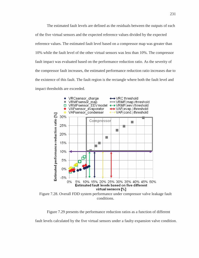
231

The estimated fault levels are defined as the residuals between the outputs of each

of the five virtual sensors and the expected reference values divided by the expected

reference values. The estimated fault level based on a compressor map was greater than

10% while the fault level of the other virtual sensors was less than 10%. The compressor

fault impact was evaluated based on the performance reduction ratio. As the severity of

the compressor fault increases, the estimated performance reduction ratio increases due to

the existence of this fault. The fault region is the rectangle where both the fault level and

impact thresholds are exceeded.

Figure 7.28. Overall FDD system performance under compressor valve leakage fault

conditions.

Figure 7.29 presents the performance reduction ratios as a function of different

fault levels calculated by the five virtual sensors under a faulty expansion valve condition.

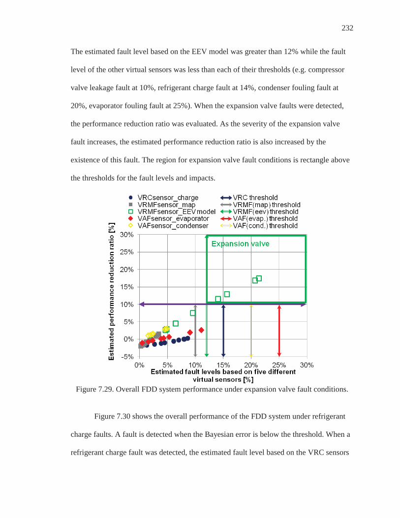
232

The estimated fault level based on the EEV model was greater than 12% while the fault

level of the other virtual sensors was less than each of their thresholds (e.g. compressor

valve leakage fault at 10%, refrigerant charge fault at 14%, condenser fouling fault at

20%, evaporator fouling fault at 25%). When the expansion valve faults were detected,

the performance reduction ratio was evaluated. As the severity of the expansion valve

fault increases, the estimated performance reduction ratio is also increased by the

existence of this fault. The region for expansion valve fault conditions is rectangle above

the thresholds for the fault levels and impacts.

Figure 7.29. Overall FDD system performance under expansion valve fault conditions.

Figure 7.30 shows the overall performance of the FDD system under refrigerant

charge faults. A fault is detected when the Bayesian error is below the threshold. When a

refrigerant charge fault was detected, the estimated fault level based on the VRC sensors

233

was greater than the threshold while the output of the other virtual sensors was less than

each of the thresholds. Three points that were higher than the threshold for the fault

detection still remained within the threshold for the performance reduction ratio. To

avoid potential system failures, however, an overcharging warning is necessary. This is

made by combining the fault detection based on Bayesian classification error and the

fault impact evaluation. The intersection of the vertical line for the performance threshold

and the horizontal line for the fault threshold can separate fault, warning, and normal

regions in the figure. The results show that the outputs of other virtual sensor are

decoupled from the refrigerant charge faults.

Figure 7.30. Overall FDD system performance under refrigerant charge faults.

Figure 7.31 shows the overall FDD system performance under evaporator fouling

faults. The threshold for fault detection was determined to be a 25% fault level. It can be

234

seen that the output of the VAF sensor for the evaporator is only influenced by the

evaporator fouling fault. The increase of the evaporator fault level is proportional to

capacity reduction and is independent of other fault levels.

Figure 7.31. Overall FDD system performance under evaporator fouling faults.

Figure 7.32 shows the overall FDD system performance under condenser fouling

faults. When condenser fouling was detected, the estimated fault level was greater than

20% while the output of the other virtual sensors was less than the thresholds. The result

shows six points that are higher than the thresholds for both fault level and performance

reduction ratio. Due to minor fault impacts, three points for condenser fouling were

below the thresholds indicating normal operation. Although two data points of the VRC

sensor were detected as faults, the performance reduction ratio was less than the threshold.

235

Figure 7.32. Overall FDD system performance under condenser fouling faults.

7.7 Overall FDD System Performance under Multiple-Simultaneous Fault Conditions

Previous FDD approaches with a fault diagnosis classifier have difficulties in

handling multiple faults because the state variables typically depend on more than one

fault along with various operating conditions. The impacts of individual faults should be

decoupled in order to handle multiple faults that occur simultaneously for accurate

diagnosis of each fault. The FDD method based on integrated virtual sensors and fault

impact can isolate a specific fault from other faults and decouple the performance

impacts of individual faults.

Figure 7.33 shows individual fault performance reduction ratios under

simultaneous condenser fouling and compressor valve leakage. The performance

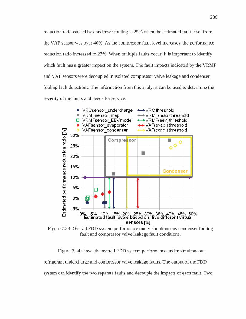
236

reduction ratio caused by condenser fouling is 25% when the estimated fault level from

the VAF sensor was over 40%. As the compressor fault level increases, the performance

reduction ratio increased to 27%. When multiple faults occur, it is important to identify

which fault has a greater impact on the system. The fault impacts indicated by the VRMF

and VAF sensors were decoupled in isolated compressor valve leakage and condenser

fouling fault detections. The information from this analysis can be used to determine the

severity of the faults and needs for service.


fault and compressor valve leakage fault conditions.

Figure 7.34 shows the overall FDD system performance under simultaneous

refrigerant undercharge and compressor valve leakage faults. The output of the FDD

system can identify the two separate faults and decouple the impacts of each fault. Two

237

vertical threshold lines for fault detection were extended to indicate fault warnings. For a

refrigerant charge fault, one data point was within the thresholds for fault detection and

performance, showing no fault. Another data point was within the threshold for

performance reduction ratio but out of the threshold for fault detection, indicating the

need for a warning signal. The rest of data points were within the fault region and were

outside both thresholds. For a compressor valve fault, as the severity of the compressor

fault increases, the predicted performance reduction ratio is increased due to the existence

of this fault. Overall, the technician could detect a charge problem based on the VRC

sensor regardless of the existence of a compressor leakage fault.

Figure 7.34. Overall FDD system performance under simultaneous refrigerant

undercharge and compressor valve leakage fault conditions.

238


condenser fouling and refrigerant fault conditions. The outputs of the VRC sensor and the

VAF sensors (condenser) are dependent on certain individual fault and are separated from

the effects of other faults. The 20% fault levels based on the VAF sensor were higher

than both expected thresholds, indicating condenser fouling. The condenser fouling

results with 12% fault level were also below the thresholds indicating normal conditions,

due to minor fault impact. Although refrigerant charge fault levels were higher than the

threshold for the fault detection, the performance impact still remained within the

threshold for the performance reduction ratio. However, an undercharged condition

potentially leads to system malfunction if it was originally caused by continuous

refrigerant leakage. Like overcharged conditions, therefore, undercharged conditions also

require a warning signal.

239


fault and refrigerant undercharge fault conditions.


evaporator fouling and refrigerant fault conditions. Overall, the evaporator fouling data

points were clearly distinguished from the normal region, which is within both thresholds,

indicating faults. All refrigerant fault data points were low in both fault detection and

performance reduction ratio, indicating normal conditions.

240

Figure 7.36. Overall FDD system performance under simultaneous evaporator fouling

fault and refrigerant undercharge fault conditions.


compressor valve leakage and refrigerant fault conditions. Although the FDD system

detected refrigerant overcharge faults, it can be seen that there are no data out of the

performance reduction threshold, indicating an overcharge warning. The compressor

leakage fault data are shown in the fault region, which is higher than both thresholds.

241


and compressor valve leakage fault conditions.


faulty expansion device and refrigerant fault conditions. The expansion fault data points

are located in the fault region except for one data point at the exact intersection of two

thresholds. This condition is also regarded as a fault. Like the previous cases, refrigerant

overcharge fault data points indicate warnings for proper system management.

242


and expansion valve fault conditions.

7.8 Summary

Laboratory tests were performed on a 4 ton RTU system to enable a complete

evaluation of FDD performance. The single-fault conditions, compressor valve leakage,

condenser and evaporator fouling, electronic expansion valve, filter/dryer restriction and

refrigerant charge fault, as well as simultaneous faults were tested in the psychrometric

chambers at the Herrick Laboratories.

The decoupling FDD method is based on integrated virtual sensors which can

isolate specific detected faults from other faults and can handle multiple simultaneous

faults. The virtual sensors showed good performance within 10% of real measurements

regardless of the different operating temperatures and faulty test conditions. A particular

243

fault would be identified if the Bayesian error between prediction from a virtual sensor

and the expected value exceeded a target error.

The decision support based on the fault energy impact model was also developed

using experimental data at different fault levels. The energy impact model was used to

provide performance degradation estimates to aid in the decision to recommend service

or other corrective action. Severe faults with more than 10% performance reduction are

apparent enough to justify the expense of servicing the system.

244

CHAPTER 8. CONCLUSION

8.1 Conclusion

The overall goal of this work was to develop and demonstrate a diagnostics

decision support tool for air conditioning systems that can enable cost effective

diagnostics solutions. Previous studies have documented typical energy degradations of

15~30% due to inadequate maintenance and service of existing faults. An automated

FDD system that can automatically detect and diagnose faults and evaluate fault impacts

has the potential for improving energy efficiency along with reducing service costs and

comfort complaints. The primary bottlenecks to diagnostic implementation in the field

are the high initial costs of additional sensors. However, the diagnostic approaches based

on virtual sensors only require low-cost physical sensors.

The impact of individual faults on capacity and energy efficiency was evaluated

for air conditioners over a wide range of operating conditions. Based on the results of this

study, refrigerant undercharging in the range of 25% can lead to an average reduction of

20% in cooling capacity. Furthermore, an undercharge of about 25% would cause an

average cost penalty of $60 per year per ton of rated capacity for typical electricity rates.

For evaporator fouling, a reduction of air flow rate by 50% decreased the average

capacity by 14%, whereas annual cost increases were $24 per ton. For condenser fouling,

245

a reduction of air flow rate by 50% decreased the average capacity by 9%, whereas the

annual cost increased by $80 per ton.

Even though various FDD studies have been carried out for air conditioner and

heat pump systems with fixed-speed compressors and fixed-orifice expansion valves,

FDD research for systems with variable-speed compressors and fans and electronic

expansion valves has been limited. In the current work, virtual sensors for variable-speed

compressors were developed to estimate mass flow rates and power consumption using

inexpensive temperature sensors and embedded models. The virtual sensors for a

variable-speed compressor can predict mass flow rates and power consumption within

RMS errors of ± 5% and ± 3%, respectively, under normal (no-fault) conditions.

A virtual refrigerant charge sensor (VRC) was extended for determining

refrigerant charge of equipment having variable-speed compressors and fans. Overall, the

original approach (model I) with tuned parameters was found to work well in estimating

the refrigerant charge for systems with a variable-speed compressor under many

operating conditions. However, for extreme test conditions such as low outdoor

temperatures and low compressor speeds, model I needed to be improved. To overcome

the limitations, the model associated with the VRC sensor was modified to include a term

involving the inlet quality to the evaporator (termed model II). Model II gave better

performance for systems with a variable-speed compressor. However, when the superheat

of the compressor was zero, neither model I nor model II could accurately predict the

charge level. Therefore, a third approach (model III) was developed that includes the

discharge superheat of the compressor. This model showed improved performance for a

246

laboratory-tested system that included a number of points with no superheat entering the

compressor.

Refrigerant mass flow rate is an important measurement for monitoring HVAC

systems. Three different virtual refrigerant mass flow (VRMF) sensors were evaluated for

estimating the refrigerant mass flow rate. The first model uses a compressor map that

relates refrigerant flow rate to measurements of condensing and evaporating saturation

temperature, and to compressor inlet temperature measurements. The second model uses

a compressor energy balance with the power consumption from a virtual compressor

power (VCP) sensor and heat loss model. The second model is relatively independent of

compressor faults and a faulty expansion valve, both of which influence mass flow rate.

The third model was developed using an empirical correlation for thermal expansion

valves (TXV) and electronic expansion valves (EEV) based on an orifice equation. The

three VRMF sensors were shown to work well in estimating the refrigerant mass flow

rate for various systems under fault-free conditions with less than 5% RMS error. Each

of the three mass flow rate estimates can be utilized to diagnose and track a loss of

compressor performance or a faulty expansion device. Virtual air flow (VAF) sensors for

condenser and evaporator fouling were also developed and evaluated in order to

characterize air flow rate effects under various faulty conditions.

To assess the impact of faults on system performance, the capacity, efficiency,

and operating cost were evaluated using data for units tested in the laboratory. Some data

were also obtained from manufacturers. The impacts of the faults were used to determine

thresholds for the FDD demonstration system. Information about capacity, power

247

consumption, and energy efficiency can be used in real-time monitoring of the economic

status of equipment and for decision support.

The performance models for capacity and power consumption for normal

conditions were developed based on manufacturer system specifications or existing

normal test data. A comparison between current estimated performance and normal

expected values was used to develop the performance reduction ratio model. The fault

impact models can determine whether a current fault, when detected, is severe enough to

justify service.

An analysis of data from a number of packaged air conditioners was conducted to

understand the impacts of faults on performance in order to set thresholds for diagnostics.

A number of virtual sensors have been developed to enable a demonstration of

diagnostics systems for RTUs and other DX air conditioners. In addition, a complete

implementation and demonstration of an AFDD system has been developed and

connected to data obtained from an RTU monitored in the field. The user interface

incorporates integrated virtual sensors to provide diagnostic outputs and performance

impacts of the fault(s) with low sensor costs. Health and economic status reports for the

equipment are generated using fault impact indices that measure the degradation in

system cooling capacity and efficiency (COP). More detailed fault information is

provided that includes the probabilities for the existence of different faults and trending

of fault indices. This statistical data are useful information in building user confidence in

the FDD system outputs.

Virtual sensors were evaluated and validated for an RTU using both laboratory

and field test data. Refrigerant charging methods specified by the manufacturer were

248

compared against indications of the VRC sensor using RTU field test data. The

comparison showed that the current approaches would have difficulty in identifying the

proper charge amount under condenser fouling conditions. However, the VRC sensor

provided accurate refrigerant charge estimates regardless of condenser fouling faults. The

VAF sensor for the condenser based on an energy balance was evaluated with field test

data. As the severity of the condenser fouling increased, the estimated air flow rate was

decreased. Condenser air flow rate reduction was found to be an independent feature for

condenser fouling.

The VRC, VRMF, and VAF sensors for a DX system have been developed and

demonstrated in Building 101 at the Navy Shipyard in Philadelphia, PA. Historical data

have been acquired during the summer seasons and the performance of the virtual sensors

was evaluated using the data filtered by a steady state detector. The performance of the

VRC sensor was estimated to be within 10% of the actual charge. Although it was not

possible to fully validate the VRMF, VCP, and VAF for condenser sensors, the outputs of

the virtual sensors showed the proper dependence on compressor and fan staging and did

not deviate from normal behavior during the course of the evaluation. A user interface for

diagnostic demonstration was developed with the status of compressors and fans, three

virtual sensors, and performance indices.

A complete diagnostic FDD system was implemented and demonstrated for a

rooftop air conditioner (RTU) that incorporates integrated virtual sensors and fault impact

evaluation for decision support. A 4 ton RTU system at the Herrick Laboratories was

tested to provide a complete evaluation of an FDD system based on virtual sensors and

fault impact models with low sensor costs. The implementation incorporates integrated

249

virtual sensors with low sensor costs to provide diagnostic outputs and the performance

impacts due to faults. The test conditions included a wide range of fault and operating

conditions with multiple simultaneous fault situations. The statistical evaluation based on

Bayesian classifiers was performed to determine reasonable fault detection thresholds for

the virtual sensors that maximize fault detection sensitivity while minimizing false alarm

rate.

Once faults are detected and the causes of the faults are identified, an assessment

of the severity of a fault is essential to the decision process and virtual sensors can be

used as inputs to this analysis. Health and economic status reports for equipment can be

generated using fault impact indices, such as capacity and energy efficiency performance

reduction ratios. In particular, the fault impact indices can be used to assess the

economics associated with servicing a unit if faults exist.

8.2 Recommendations

It is recommended that additional research and development be carried out to add

capability to FDD methods. These capabilities could include estimates of energy fault

impact and service cost impacts. The economic payback should be estimated using

projections of implementation costs and estimated fault impacts. It is also important to

define reasonable thresholds based on economic benefit by comparing service costs with

economic fault impacts for appropriate fault detection and diagnosis. More investigations

are necessary to optimize FDD systems with economic evaluation.

To accurately and robustly determine refrigerant charge level with operating

refrigerant overcharge, VRC sensors are needed which provide better charge predictions

250

at these conditions. For severe undercharge or condenser fouling conditions, the two-

phase refrigerant inlet state led to inaccurate estimates of the VAF and VRMF sensors.

This occurred because a quality of zero had to be used for property calculations at these

conditions, which contributes to possible false alarms and sensitivity loss. Additional

research and development is recommended to provide better estimation in those cases.

Another necessary implementation of an FDD system is one which can consider

systems that incorporate multiple evaporators and variable-speed compressors. As the use

of systems with multiple evaporators has been increasing in the world market, tests

extending the FDD method based on virtual sensors to these systems are recommended.

When the FDD system is extended to systems with multiple evaporators, some

modifications and adjustments should be required for accurate estimation. Further

performance evaluations are also recommended for systems with variable-speed

compressors.

251

LIST OF REFERENCES

251

LIST OF REFERENCES

ADM, 2009, Market “Assessment and field M&V Study for Comprehensive Packaged A/C Systems Program”, Final Report.

Ahan, Y. C. Cheong., Y.G, and Lee, J. K., 2006, “An Experimental Study of the Air-Side

Particulate Fouling in Fin-and-Tube Heat Exchangers of Air Conditioners”, International Refrigerant and Air conditioning Conference, Vol.20, No. 5, Page 873-877.

ANSI/ARI Standard 540-99, 2004, “Standard for Performance Rating of Positive

Displacement Refrigerant Compressors and Compressor Units”, Air-Conditioning, Heating, and Refrigeration Institute, Arlington, VA 22201, U.S.A.

Aprea C., Mastrullo R. and Renno C., 2004, Fuzzy Control of the Compressor Speed in a

Refrigeration Plant, International Journal of Refrigeration, Vol.27, No. 6, Page 639-649.

Armstrong, P.R., Laughman, C.R., Leeb, S.B., Norford L.K., 2006, “Detection of

Rooftop Cooling Unit Faults Based on Electrical Measurements”, HVAC&R Research, Vol.12, No. 1, Page 151-175.

ASHRAE, 2010, ASHRAE Standard 116, “Methods of Testing for Rating Seasonal

Efficiency of Unitary Air-Conditioners and Heat pumps”, American Society of Heating, Refrigerating, and Air-Conditioning engineers, Inc, Atlanta, GA.

Bach, C., 2010, “A Virtual EXV Mass Flow Sensor for Applications with Two-Phase

Flow Inlet Conditions”, International Refrigerant and Air conditioning Conference, No. 2122.

Blasnik, M., Downey, T., Proctor, J. and Peterson, G., 1996, “Assessment of HVAC

Installations in New Homes in APS Service Territory”, Proctor Engineering Group Report for Arizona Public Service Company

252

Brambley, M., Pratt, R., Chassin, D., Katipamula, S. and Hatley, D., 1998, “Automated Diagnostics for Outdoor Air Ventilation and Economizers”, ASHRAE Journal, Vol. 40, No.10, Page 49-55.

Braun, J.E., 2003, “Automated Fault Detection and Diagnostics for Vapor Compression

Equipment”, ASME Journal of Solar Energy Engineering, Vol.125, Page 266-274.

Breuker, M. S. and Braun, J. E., 1998a, “Evaluating the performance of a fault detection

and diagnostic system for vapor compression equipment”, HVAC&R Research, Vol. 4, No.4, Page 401-425.

Breuker, M. S. and Braun, J. E., 1998b, “Common faults and their impacts for rooftop air

conditioner, HVAC&R Research”, Vol. 4, No.3, Page 303-318. Browne M .W. and Bansal P. K., 2002, “Transient Simulation of Vapor Compression

Packaged liquid chillers”, International Journal of Refrigeration, Vol.25, Page 597-610.

Chen, B. and J.E. Braun., 2001, “Simple Rule-Based Methods for Fault Detection and

Diagnostics Applied to Packaged Air Conditioners”, ASHRAE Trans., Vol.107, Part 1.

Choi, J. M. and Kim, Y. C., 2002. “The Effect of Improper Refrigerant Charge on the

Performance of a Heat Pump with an Electronic Expansion Valve and Capillary tube”, Energy, Vol.27, Page 391-404.

Cowan, A., 2004, “Review of recent commercial rooftop unit field studies in the Pacific

Northwest and California”. Northwest Power and Conservation Council and Regional Technical Forum, Portland, Oregon.

Dixon, K., Dolan, J., Huang, W., Paredis, C. and Khosla, P., 1999, "RAVE: A Real and

Virtual Environment for Multiple Mobile Robot Systems," in Proceedings of the IEEE/RSJ International Conference on Intelligent Robots and Systems, Vol.3, Page 1360-1367.

Downey, T. and Proctor, J., 2002, “What Can 13,000 Air Conditioners Tell Us?” In

Proceedings of the ACEEE 2002, Summer Study on Energy Efficiency in Buildings, Vol.1, Page 53-68. Washington D.C.

253

Energy Information Agency (EIA), 1999, “Commercial Buildings Energy Consumption Survey”, Available online: http://www.eia.doe.gov/emeu/cbecs/tables.

Energy Information Agency (EIA), 2001, “Residential Energy Consumption Survey”,

Available online: http://www.eia.doe.gov/emeu/recs/byfuels. Energy Information Agency (EIA), 2003, “Commercial Buildings Energy Consumption

Survey 2003”, Available online: http://205.254.135.7/emeu/cbecs/cbecs2003/detailed_tables_2003/detailed_tables_2003.html#consumexpen03

Epstein, N., 1978, “Fouling in Heat Exchangers”, Sixth International Heat Transfer

Conference, Vol.6, Page 235-253. Hemisphere, Washington, D.C. Farzad, M., 1990, “Modeling the Effects of Refrigerant Charging on Air Conditioner

Performance Characteristics for Three Expansion Devices,” Ph.D., Department of Mechanical Engineering, Texas A&M University, TX.

Fukunaga, K., 1990, “Introduction to Statistical Pattern Recognition”, Academic Press,

West Lafayette, IN. Goswami D. Y., 2001, “Effect of Refrigerant Charge on the Performance of Air

Conditioning Systems”, International Journal of Energy Research, Vol.25, No. 8, Page 741-.750

Ding G., 2007, “Recent Developments in Simulation Techniques for Vapor-Compression

Refrigeration Systems”, International Journal of Refrigeration, Vol.30, No. 7, Page 1119-1133.

Gustafsson, F, 1998, “Estimation and Change Detection of Tire-Road Friction Using the

Wheel Slip”, IEEE Control System Magazine, Vol.18, No.4, Page 42-49.

Harms, T. M., 2002, “Charge Inventory System Modeling and Validation for Unitary Air Conditioners”, Ph.D. Thesis, Report No. 5288-2, Purdue University, IN.

254

Healy, W., 2010, “Vapor Compression Equipment Sensors and Energy Monitoring Systems, Vapor Compression Equipment America Meeting on Diagnostic Measurement and Performance Feedback for Residential Space Conditioning Equipment”, National Institute of Standards and Technology, Gaithersburg, MD.

Heredia, G and Ollero, A., 2010, "Virtual Sensor for Failure Detection, Identification and Recovery in the transition Phase of a Morphing Aircraft," Sensors, Vol.10, No.3, Page 2188-2201.

Hrnjak, P. S., Lenger, M. J. and Jacobi, A. M., 1998, “Superheat Stability of an Evaporator and Thermostatic Expansion Valve”, air conditioning and refrigeration center, University of Illinois at Urbana-Champaign.

Inatsu, H., H. Matsuo, K. Fujiwara, K. Yamada, and K. Nishizawa, 1992, “Development of Refrigerant Monitoring Systems for Automotive Air-Conditioning Systems,” Society of Automotive Engineers, SAE Paper No. 920212.

J. Stéphant, A. Charara, and D. Meizel, 2004, "Virtual Sensor: Application to Vehicle Sideslip Angle and Transversal Forces," IEEE Transactions on Industrial Electronics, vol. 51, no. 2, pp. 278-289, April 2004.

Katipamula, S. and Brambley, M. R., 2005, “Methods for Fault Detection, Diagnostics, and Prognostics for Vapor Compression Equipment Systems, A Review, Part I”, HVAR&R Research, Vol. 11, No. 1, Page 3-25.

Kabadayi. S, Pridgen. A, and Julien. C, 2006, “Virtual Sensors: Abstracting Data from Physical Sensors, International Symposium on a World of Wireless”, Mobile and Multimedia Networks, Page 587-592.

Keir, M.C. and Alleyne, 2006, “Dynamic Modeling, Control, and Fault Detection in Vapor Compression Systems”, University of Illinois, Illinois, USA.

Kim, W. H. and Braun, J. E., 2012a, “Performance Evaluation of a Virtual Refrigerant Charge Sensor”, International Journal of Refrigeration, Vol.36, No.3, Page 1130-1141 .

255

Kim, W. H. and Braun, J. E., 2012b, “Evaluation of virtual refrigerant mass flow sensors”, International Refrigerant and Air conditioning Conference, No. 2299.

Kim, W. H. and Braun, J. E., 2012c, “Evaluation of the Impact of Refrigerant Charge on

Air conditioner and Heat pump performance”, International Journal of Refrigeration, Vol.35, No.7, Page 1805-1814.

Kim, K. C. and Cho, D. G., 2005, “An experimental study on the performance of inverter

heat pump with a variation of frequency and refrigerant charging rate”, Korea Journal of Refrigerant, Vol.15, Page 187-205.

Kim, M. and Kim, M. S., 2005, “Performance investigation of a variable-speed vapor

compression system for fault detection and diagnosis”, International Journal of Refrigerant, Vol. 28, Page 481-488.

Kim, M. and Payne, V., 2008, “Cooling Mode Fault Detection and Diagnosis Method for

a Residential Heat Pump”, NIST Special Publication 1087, National Institute of Standards and Technology, Gaithersburg, MD.

Klein, S. A. and Alvarado, F. L., 2009, Engineering Equation Solver (EES), F-Chart

Software, Madison. WI, Available online: www.fchart.com. Kline, S. J. and McClintock, F. A., 1953, “Describing uncertainties in single-sample

experiments,” Mechanical Engineering, Vol.75, Page 3-8. Krafthefer, B. C., Rask, D. R. and Bonne, U., 1987, “Air Conditioning and Heat pump

Operating Cost Savings by Maintaining Coil Cleanliness”, ASHRAE Transactions, Vol. 93, No.1, Page.1458-73.

Kumar, R., Shin, J., Iftode, L. and Rama chandran, U., 2008, "Mobile Virtual Sensors: A

Scalable Programming and Execution Framework for Smart Surveillance," in Proceedings of the 5th Workshop on Embedded Network Sensors.

Lemmon, E. W., McLinden, M. O. and Huber, M. L., 2002, REFPROP: Reference Fluid

Thermodynamic and Transport Properties, NIST Standard Database 23, version 7.0

256

Li, H. and Braun, J. E., 2007a, “Decoupling Features and Virtual Sensors for Diagnosis of Faults in Vapor Compression Air Conditioners”. International Journal of Refrigeration, Vol. 30, No. 3, Page 546-564

Li, H. and Braun, J. E., 2007b, “A Methodology for Diagnosing Multiple-Simultaneous

Faults in Vapor Compression Air Conditioners”. HVAC&R Research, Vol. 13, No.2, Page 369-395.

Li, H. and Braun, J.E., 2007c, "Economic Evaluation of the Benefits Associated with

Application of Automated Fault Detection and Diagnosis in Rooftop Air Conditioners," ASHRAE Transactions, Vol. 113, Pt. 2, Page 200-210.

Li, H. and Braun, J. E., 2008, “A method for Modeling Adjustable Throat-Area

Expansion Valves Using Manufacturers' Rating Data”. HVAC&R Research, Vol.14, No.4, Page 581-598

Li, H. and Braun, J. E., 2009a, “Development, Evaluation, and Demonstration of a

Virtual Refrigerant Charge Sensor.” HVAC&R Research, Vol. 15(1), Page 117-136

Li, H. and Braun, J. E., 2009b, “Virtual Refrigerant Pressure Sensors for Use in

Monitoring and Fault Diagnosis of Vapor-Compression Equipment”, HVAC&R Research, Vol. 15, No. 3, Page 597-616.

Li, H., and Braun, J. E., 2009c, Decoupling Features for Diagnosis of Reversing and

Check Valve Faults in Heat Pumps”, International Journal of Refrigeration, Vol. 32, Page 316-326.

Li, Y., Braun, J.E., and Groll, E.A., 2007, “The Impact of Evaporator Fouling and

Filtration on the Performance of Packaged Air Conditioners”, International Journal of Refrigeration, Vol. 30, Page 506-514.

Lichuan Liu., Kuo, S. M., and Meng Chu Zhou., 2009, “Virtual Sensing Techniques and

their Applications”, International Conference on Networking, Sensing and Control, Page 31-36.

Mei, V. C., Chen, F. C., and Gao, Z., 2003., “Development of Refrigerant Charge

Indicator and Dirty Air Filter Sensor”, Oak Ridge National Laboratory.

257

Messenger, M., 2008, “Strategic Plan to Reduce the Energy Impact of Air Conditioners”, CEC-400-2008-010.

Navarro-Esbry J., Berbegall V., Verdu G., Cabello R. and Lopis R., 2007, “A low data

requirement model of a variable-speed vapor compression refrigeration system based on neural networks”, International Journal of Refrigeration, Vol. 30, Page 1452-1459.

New Buildings Institute, 2003, “Integrated Energy Systems: Productivity & Building

Science”, Available online: http://www.energy.ca.gov/pier/project_reports/ Nyika, S., 2012, “Experimental Evaluation of Variable speed residential ductless heat

pumps”, Thesis, Purdue University Park, C., Cho, H. and Kim, Y., 2007, “Mass flow characteristics and empirical modeling

of R22 AND R410A flowing through electronic expansion valves”, International Journal of Refrigeration, Vol. 3, Page 1-7.

Park Y.C., Kim Y.C., and Min M.K., 2001, “Performance Analysis on a Multi-Type

Inverter Air Conditioner”, Energy Conversion Mgmt, Vol.42, Page 1607-1621. Payne, W. V., Kim, M. S., Yoon, S. H., and Domanski, P. A., 2008, “Cooling Mode Fault

Detection and Diagnosis Method for a Residential Heat Pump”, NIST SP 1087; NIST Special Publication, Page1087-98.

Proctor, J., 1997, “Field Measurements of New Residential Air Conditioners in Phoenix,

Arizona”, ASHRAE Transactions, Vol.103, No.1, Page 406-415. Proctor, J., 1998, “Monitored in-situ Performance of Residential Air-Conditioning

Systems”, ASHRAE Transactions, Vol. 104, No.1, Page 1833-1840. Proctor, J. and Downey, T., 1995, “Heat pump and air conditioner performance.”

Handout from oral presentation. Affordable Comfort Conference, Pittsburgh, PA. Quereshi ,T. Q. and Tassou, S.A., 1996, “Variable-speed capacity controls in

refrigeration system”, Applied Thermal Engng, Vol. 16, No.2, Page 103-113.

258

Rallo, R., Ferre-Gine, J., and Arenas, A., 2002, “Neural virtual sensor for the inferential prediction of product quality from process variables” Computers and Chemical Engineering, Vol. 26, Page 1735-1754.

Reddy, T. A., 2006, “Evaluation and assessment of fault detection and diagnostic

methods for centrifugal chillers—Phase II.” GA Final project report of ASHRAE Research Project, GA, RP-1275.

Rice, C. A., 1987, "The Effect of Void Fraction Correlation and Heat Flux Assumption

on Refrigerant Charge Inventory Predictions," ASHRAE Transactions, Vol. 93, No.1, Page 341- 367.

Rossi, T. M. and Braun, J. E., 1997, “A statistical, rule-based fault detection and

diagnostic method for vapor compression air conditioners”, HVAC&R Research, Vol. 3, No.1, Page 19–37.

Shanwei, M., Chuan, Z., Jiangping, C., and Zhiujiu, C., 2005, “Experimental research on

refrigerant mass flow coefficient of electronic expansion valve”, Applied Thermal Eng., Vol. 25, Page 2351-2366.

Shao, S., Wenxing, S. and Chen, H., 2004, “Performance Representation of Variable-

Speed Compressor for Inverter Air Conditioners based on Experimental Data.”, International Journal of Refrigeration, Vol. 27, No,8, Page 805-815.

Siegel, J. and Wray, C. 2002. “An Evaluation of Superheat-Based Refrigerant Charge

Diagnostics for Residential Cooling Systems”, ASHRAE Transactions, Vol. 108, part 2, Page 965-975.

Siegel, J. A. and Nazaroff, W. W.,2003, “Predicting Particle Deposition on HVAC Heat

Exchangers”, Atmospheric Environment”, Vol. 37, Page 5587-5596. U.S. Department of Energy, 2010, “Energy Efficiency Trends in Residential and

Commercial Buildings”, Washington, DC: United States Department of Energy. Wagner, J. and R. Shoureshi., 1992. “Failure Detection Diagnostics for Thermofluid

Systems”, Journal of Dynamic Systems, Measurement, and Control”, Vol. 114, No.3, Page 699-706.

259

Wichman, A. and Braun. J. E., 2009, “A Smart Mixed-Air Temperature Sensor”, HVAR&R Research, Vol. 15, No.1, Page 101-115

Yoshimura, M. and I. Noboru.,1989., Effective Diagnosis Methods for Air-Conditioning

Equipment in Telecommunications Buildings, In Proceedings of INTELEC 89: The Eleventh International Telecommunications Energy Conference, Firenze, Vol.21, No.1,Page 1-7.

Yu, D., Li, H. and Braun, J. E., 2011, “A Review of Virtual Sensing Technology and

Application in Vapor compression equipment Systems.” HVAC&R Research, Vol 17, Page 619-645.

Zivi, S. M., 1964, “Estimation of Steady-State Steam Void-Fraction by Means of the

Principle of Minimum Entropy Production.” Journal of Heat Transfer, Vol. 86, Page 247-252.

260

APPENDIX

260

APPENDIX: PARAMETERS OF VIRTUAL SENSORS

A.1 RTU system I obtained by UTRC laboratory test (Chapter 6) A.1.1 VRC sensor model 1 and 3 based on default parameters.

10011[%] ,/,1,arg ratedshshscshratedscscch

modelech TTKTTK

m

10011

[%]

,/

,,,/,/,

3,arg

rateddshshscdsh

ratedinevapinevapscxratedshshscshratedscsc

ch

modelech

TTK

TxKTTKTT

K

m

Rated values for VRC sensors Parameters for VRC sensors

ratedscT , ratedshT , ratedinevapx ,, rateddshT , chK

1 scshK / scxK / scdshK /

Model 1 8.23 C 4.70 C 0.021 -0.010

Model 3 8.23 C 4.70 C 0.21 56.79 C 0.022 -0.006 0.012 -0.003

A.1.2 VCP sensor

)([%]

29

28

37

365

24

23210

ionspecificatsystempowercompressorratedTTaTTaTaTaTTaTaTaTaTaa

W ecceeecceeccVCP

Parameters of VCP sensor a0 a1 a2 a3 a4 a5 a6 a7 a8 a9

-17996 84.098 0.162 16208.659 489.234 2.416 553.329 -2.332 -3.549 0.020 A.1.3 VRMF sensors

A.1.3.1 VRMF sensor 1 based on compressor map

rateflowmasstrefrigeranratedTTbTTbTbTbTTbTbTbTbTbb

W ecceeecceeccsuctionVRMF1

29

28

37

365

24

23210[%]

Parameters of VCP sensor b0 b1 b2 b3 b4 b5 b6 b7 b8 b9

-161.40 4.036 -0.031 -355.36 14.329 0.108 2.030 0.030 0.362 0.075

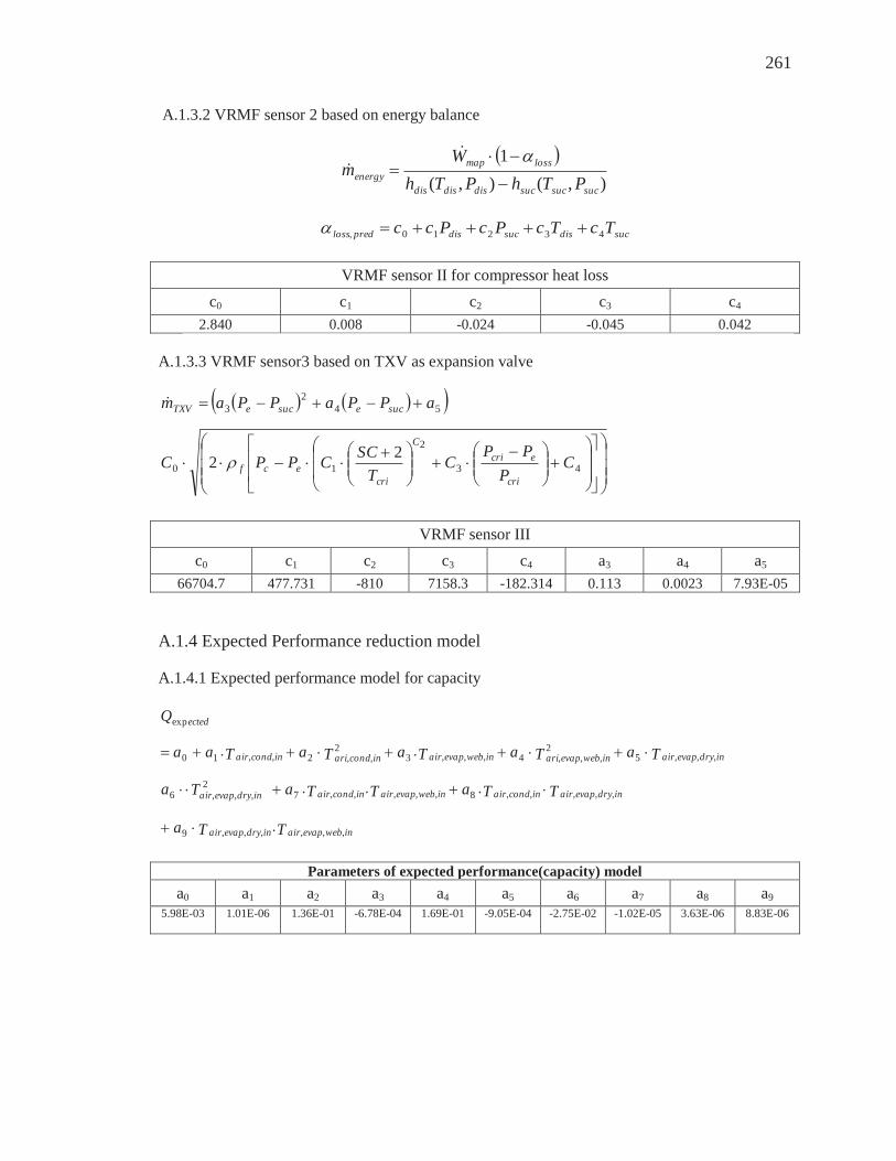
261

A.1.3.2 VRMF sensor 2 based on energy balance

),(),(1

sucsucsucdisdisdis

lossmapenergy PThPTh

Wm

sucdissucdispredloss TcTcPcPcc 43210,

VRMF sensor II for compressor heat loss c0 c1 c2 c3 c4

2.840 0.008 -0.024 -0.045 0.042

A.1.3.3 VRMF sensor3 based on TXV as expansion valve

43

2

10

542

3

22 CP

PPC

TSCCPPC

aPPaPPam

cri

ecriC

criecf

sucesuceTXV

VRMF sensor III

c0 c1 c2 c3 c4 a3 a4 a5 66704.7 477.731 -810 7158.3 -182.314 0.113 0.0023 7.93E-05

A.1.4 Expected Performance reduction model

A.1.4.1 Expected performance model for capacity

TTa

TTaTTaTa

TaTaTaTaTaa

Q

inwebevapairindryevapair

indryevapairincondairinwebevapairincondairindryevapair

indryevapairinwebevapariinwebevapairincondariincondair

ected

,,,,,,9

,,,,,8,,,,,72

,,,6

,,,52

,,,4,,,32

,,2,,10

exp

Parameters of expected performance(capacity) model a0 a1 a2 a3 a4 a5 a6 a7 a8 a9

5.98E-03 1.01E-06 1.36E-01 -6.78E-04 1.69E-01 -9.05E-04 -2.75E-02 -1.02E-05 3.63E-06 8.83E-06

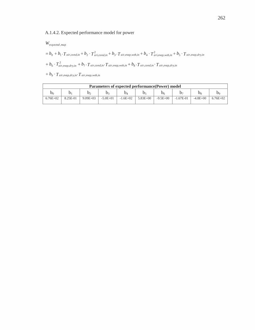
262

A.1.4.2. Expected performance model for power

TTb

TTbTTbTb

TbTbTbTbTbb

W




mapected

,,,,,,9

,,,,,8,,,,,72

,,,6

,,,52

,,,4,,,32

,,2,,10

,exp

Parameters of expected performance(Power) model b0 b1 b2 b3 b4 b5 b6 b7 b8 b9

6.76E+02 8.25E-01 9.09E+03 -5.0E+01 -1.6E+02 5.83E+00 -9.5E+00 -1.67E-01 -4.8E+00 6.76E+02

263

A.2 RTU system II obtained by UTRC field test (Chapter 6) A.2.1 VRC sensor model 1 and 3 based on default parameters.


modelech TTKTTK

m

10011

[%]

,/

,,,/,/,

3,arg

rateddshshscdsh


ch

modelech

TTK

TxKTTKTT

K

m




Model 1 8.23 C 4.74 C 2.06E-02 1.01E-02

Model 3 8.23 C 4.74 C 0.018 56.8 C 2.18E-02 5.73E-03 8.93E-01 2.82E-03

A.2.2 VCP sensor

)([%]

29

28

37

365

24

23210


W ecceeecceeccVCP


-7.22E + 02

6.32E+01

-5.23E-01

3.03E-03

-2.82E +01

2.23E-01

1.04E-03

6.61E-01

1.52E-03

-4.02E-03

A.2.3 VRMF sensors




29

28

37

365

24

23210[%]


2.82 E+02

1.09 E+00

-4.32 E-03

-4.66 E-05

8.68 E+00

7.28 E-02

4.17 E-04

-3.66 E-02

6.08E-02

3.00E-04

264


),(),(1

sucsucsucdisdisdis


Wm



-6.22E-01 -5.72E-03 9.33E-03 2.2E-02 -1.88E-02


max542

3 maPPaPPam sucesuceTXV

PCP

PPPC

TSCPCPCCm f

cri

ecrief

criefcf 43210max

2

VRMF sensor III

c0 c1 c2 c3 c4 a3 a4 a5 7.82E+01 2.65E-05 -6.87E-03 -1.48E-01 1.29E-01 1.04E+00 -2.22E-03 3.31E-05


A.2.4.1 Expected performance model for capacity ( ectedQexp )

TTa

TTaTTaTa

TaTaTaTaTaa

Q




ected

,,,,,,9

,,,,,8,,,,,72

,,,6

,,,52

,,,4,,,32

,,2,,10

exp


-3.51E +02

1.21E+01

-1.84E-01

-1.28E +01

-4.61E-02

9.90E+00

-2.61E-01

5.91E-02

1.88E-01

2.12E-01

265

A.2.4.2. Expected performance model for power ( ectedWexp )

TTb

TTbTTbTb

TbTbTbTbTbb

W




mapected

,,,,,,9

,,,,,8,,,,,72

,,,6

,,,52

,,,4,,,32

,,2,,10

,exp


7.20E +01

-1.34E +00

7.51E-03

6.33E-01

-1.04E-02

-1.00E +00

8.19E-03

9.34E-03

-4.62E-03

1.23E-03

266

A.3 Building 101 for DX3 system circuit A/B (Chapter 6) A.3.1 VRC sensor based on tuned parameters

10011[%] ,/,,arg ratedshshscshratedscscch

currentech TTKTTK

m

RTU1 system Parameters

ratedscT , ratedshT , chK

1 scshK /

Stage 1 26 C 23 C

( TXV ) 0.0219 0.0064 Stage 2 21 C

Stage 3 15 C A.3.2 VAF sensor for condenser

),(),(1

,sucsucsucdisdisdis

lossmeasuredenergyref PThPTh

Wm

1.0, predloss

condairP

acond

icaoca

inliinliinliquiddisdisdisenergyrefpredicted C

vTT

TPhTPhmV

,,

,

,,

,,,, ,,

A.3.3 Capacity and energy efficiency based on virtual sensors

outliquidsatcondsatcondoutliquidoutevapsatevapsatevapoutevapmappredicted TTPhTTPhmQ ,,,,,,,, ),(),(

map

predictedpredicted W

QCOP

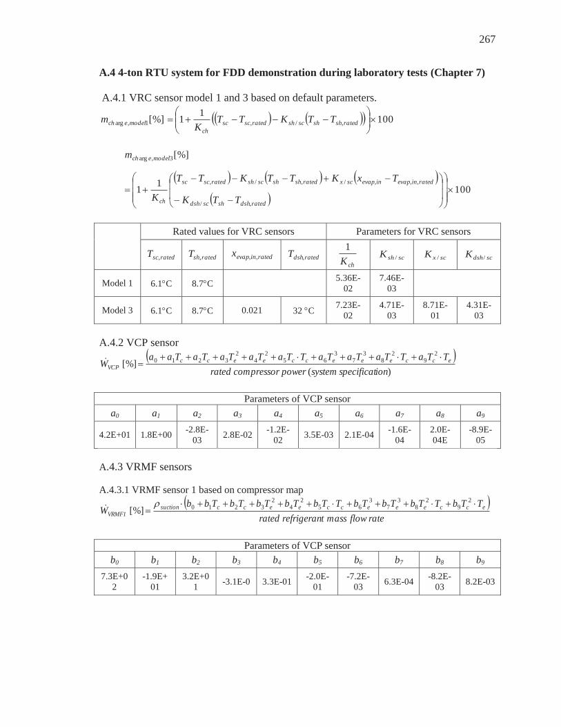
267

A.4 4-ton RTU system for FDD demonstration during laboratory tests (Chapter 7) A.4.1 VRC sensor model 1 and 3 based on default parameters.


modelech TTKTTK

m

10011

[%]

,/

,,,/,/,

3,arg

rateddshshscdsh


ch

modelech

TTK

TxKTTKTT

K

m




Model 1 6.1 C 8.7 C 5.36E-02

7.46E-03

Model 3 6.1 C 8.7 C 0.021 32 C 7.23E-02

4.71E-03

8.71E-01

4.31E-03

A.4.2 VCP sensor

)([%]

29

28

37

365

24

23210


W ecceeecceeccVCP


4.2E+01 1.8E+00 -2.8E-03 2.8E-02 -1.2E-

02 3.5E-03 2.1E-04 -1.6E-04

2.0E-04E

-8.9E-05

A.4.3 VRMF sensors




29

28

37

365

24

23210[%]


7.3E+02

-1.9E+ 01

3.2E+01 -3.1E-0 3.3E-01 -2.0E-

01 -7.2E-

03 6.3E-04 -8.2E-03 8.2E-03

268


),(),(1

sucsucsucdisdisdis


Wm



-8.7E-01 -1.6E-04 1.4E-03 -6.3E-03 5.4E-03


maxmax

2

2

max1 m

EEVSTEPEEVSTEP

DEEVSTEP

EEVSTEPDm currentcurrent

EEV

efcri

ecrief

criefcf PC

PPP

PCT

SCPCPCCm 43210max2

VRMF sensor III

c0 c1 c2 c3 c4 D1 D2 D3 -2.1E+01 2.61E-03 -2.99E-03 -6.72E-05 1.63E-02 2.33E+02 -2.18E+02 0


A.4.4.1Expected performance model for capacity ( ectedQexp )

TTa

TTaTTaTa

TaTaTaTaTaa

Q




ected

,,,,,,9

,,,,,8,,,,,72

,,,6

,,,52

,,,4,,,32

,,2,,10

exp


-4.5E+0 -9.3E-01 4.1E-01 1.1E-01 1.4E-01 7.25E-

02 -0.393 7.22E-02

-2.18E-02

-4.57E-03

269

A.4.4.2. Expected performance model for power ( ectedWexp )

TTb

TTbTTbTb

TbTbTbTbTbb

W




mapected

,,,,,,9

,,,,,8,,,,,72

,,,6

,,,52

,,,4,,,32

,,2,,10

,exp


1.7E+0 -1.9E-01

-1.7E-03

-1.5E-02 1.0E-03 7.65E-

02 9.15E-

04 7.64E-

03 -6.09E-

04 -2.62E-

03

270

VITA

270

VITA

Woohyun Kim Mechanical Engineering, Ray W. Herrick Laboratories

Graduate School, Purdue University

Education B.S., Mechanical Engineering, 1998, Sung Kyun Kwan University, Seoul, Korea M.S., Mechanical Engineering, 2000, Sung Kyun Kwan University, Seoul, Korea M.S., Mechanical Engineering, 2009, Purdue University, West Lafayette, Indiana Ph.D., Mechanical Engineering, 2013, Purdue University, West Lafayette, Indiana Research Interests I had been focused on the diagnostic control for the last six years at Purdue University. I developed the diagnostic and decision support systems for the Energy Efficient buildings. .

Fault Detection And Diagnosis For Air Conditioners And Heat ...

Documents