Fast Tridiagonal Solvers on GPU - pdfs.semanticscholar.org

Fast Tridiagonal Solvers on GPU

Yao Zhang

John Owens

UC Davis

Jonathan Cohen

NVIDIA

GPU Technology Conference 2009

Outline

• Introduction

• Algorithms

– Design algorithms for GPU architecture

• Performance

– Bottleneck-based vs. Component-based performance model

• Summary

What is a tridiagonal system?

What is it used for?

• Scientific and engineering computing

– Alternating direction implicit (ADI) methods

– Numerical ocean models

– Semi-coarsening for multi-grid solvers

– Spectral Poisson Solvers

– Cubic Spline Approximation

• Video games and computer-animated films

– Depth of field blurs

– Fluid simulation

A Classic Serial Algorithm

• Gaussian elimination in tridiagonal case (Thomas algorithm)

Phase 1: Forward EliminationPhase 2: Backward Substitution

Parallel Algorithms

• Coarse-grained algorithms (multi-core CPU)

– Two-way Gaussian elimination

– Sub-structuring method

• Fine-grained algorithms (many-core GPU)

– Cyclic Reduction (CR)

– Parallel Cyclic Reduction (PCR)

– Recursive Doubling (RD)

– Hybrid CR-PCR algorithm

A set of equations

mapped to one thread

A single equation

mapped to one thread

A little history

• Parallel tridiagonal solvers since 1960s:

– Vector machines: Illiac IV, CDC STAR-100, and Cray-1

– Message passing architectures: Intel iPSC, and Cray T3E

– And GPU as well!

Two Applications on GPU

Depth of field blur, Michael Kass et al. Shallow water simulation

OpenGL and Shader language CUDA

Cyclic reduction Cyclic reduction

20072006

Cyclic Reduction (CR)

Forward

Reduction

Backward

Substitution

8-unknown system

4-unknown system

2-unknown system

Solve 2 unknowns

Solve the rest 2 unknowns

Solve the rest 4 unknowns

2 threads working4 threads working1 thread working

2*log2 (8)-1 = 2*3 -1 = 5 steps

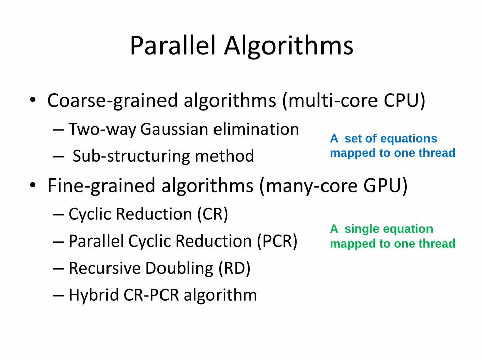
Parallel Cyclic Reduction (PCR)

Forward

Reduction

4 threads working

log2 (8) = 3 steps

One 8-unknown system

Two 4-unknown systems

Four 2-unknown systems

Solve all unknowns

Hybrid Algorithm (1)

• CR

– Every step we reduce the system size by half (Good)

– Some processing cores stay idle if the system size is smaller than the number of cores (Bad)

– Needs more steps to finish (Bad)

• PCR

– Fewer steps required (Good)

– Same amount of work for all steps (Bad)

Hybrid Algorithm (2)

System size reduced at the beginning

No idle processors

Fewer algorithmic steps

Switch to PCR

Switch back to CR

Even more beneficial because of:

bank conflicts

control overhead

GPU Implementation (1)

• Linear systems mapped to multiprocessors (blocks)

• Equations mapped to processors (threads)

GPU Implementation (2)

• Storage need: 5 arrays = 3 diagonals + 1 solution vector + 1 right hand side

• All data resides in shared memory if it fits

• Use contiguously ordered threads to avoid unnecessary divergent branches

• In-place data storage

– Efficient, but introduce bank conflicts to CR

Performance Results – Test Platform

• 2.5 GHz Intel Core 2 Q9300 quad-core CPU

• GTX 280 graphics card with 1 GB video memory

• CUDA 2.0

• CentOS 5 Linux operating system

Performance Results

Time

(milliseconds)

PCI-E: CPU-GPU data transfer

MT GE: multi-threaded CPU Gaussian Elimination

GEP: CPU Gaussian Elimination with pivoting (from LAPACK)

1.07 0.53 0.42

4.085.24

9.30

11.8

0

2

4

6

8

10

12

14

CR PCR Hybrid PCI-E MT GE GE GEP

Solve 512 systems of 512 unknowns

CR

PCR

Hybrid

PCI-E

MT GE

GE

GEP

2.5x 1.3x

12x

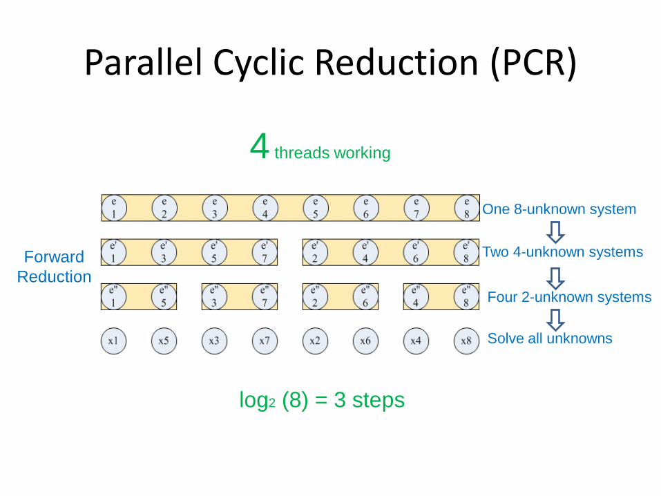
Performance Analysis

• Factors that determine performance

– Global/shared memory accesses

– Bank conflicts

– Computational complexity

– Overhead for synchronization and loop control

Bottleneck vs. Pie slice

Performance = min(factor1, factor2, …) Performance = sum(factor1, factor2, …)

Performance Measure

A manual differential method

time1

time2

time3time3-time2

time2-time1

time1

Control Overhead

0

0.005

0.01

0.015

0.02

0.025

0.03

0.035

256 128 64 32 16 8 4 2

CR: Forward Reduction

Time

(milliseconds)

# of threads running:

Control and

synchronization

overhead

A step is very

expensive in

terms of control

Step: 1 2 3 4 5 6 7 8

Time doesn’t decrease anymore,

because GPU vector length is 32 (warp size)

Enforce a stride of one to avoid bank conflicts

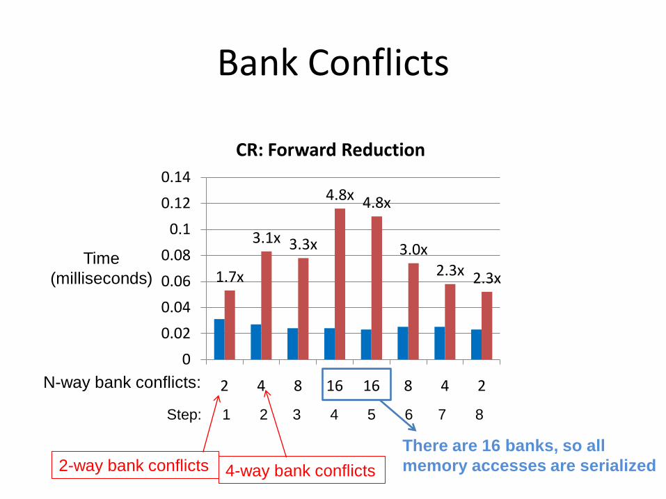
Bank Conflicts

1.7x

3.1x 3.3x

4.8x 4.8x

3.0x

2.3x 2.3x

0

0.02

0.04

0.06

0.08

0.1

0.12

0.14

2 4 8 16 16 8 4 2

CR: Forward Reduction

There are 16 banks, so all

memory accesses are serialized

Time

(milliseconds)

N-way bank conflicts:

Step: 1 2 3 4 5 6 7 8

2-way bank conflicts 4-way bank conflicts

CR vs. PCR (1)

0

0.02

0.04

0.06

0.08

0.1

0.12

0.14

M 1 2 3 4 5 6 7 8 S 1 2 3 4 5 6 7 8

Solve 512 systems of 512 unknowns (Time Breakdown)

PCR

CR

Backward SubstitutionForward Reduction

Solve 2-unknown systemsGlobal memory

Time

(milliseconds)0.53 ms

1.07 ms

CR vs. PCR (2)

0.11 20%

47 GB/s

0.16 30%

883 GB/s

0.27 50% 102

GFLOPS

PCR

Global Shared Computation

0.19%

49 GB/s

0.69 65%

33 GB/s

0.27 26%16

GFLOPS

CR

Global Shared Computation

Pros: O(n)

Cons: more steps (control

overhead), bank conflicts

Pros: fewer steps, no bank

conflicts

Cons: O(nlogn)

Pitfalls

• The higher computation rate and sustained bandwidth, the better

– They may have different algorithm complexity

• The lower algorithm complexity, the better

– What if there is considerable amount of control overhead, or bank conflicts, or low hardware utilization

PCR vs Hybrid

• Make tradeoffs between the computation, memory access, and control

– The earlier you switch from CR to PCR

• The fewer bank conflicts, the fewer algorithmic steps

• But more work

Hybrid Solver – Sweet Point

0

0.2

0.4

0.6

0.8

1

1.2

2 4 8 16 32 64 128 256 512

Optimal performance of hybrid solverSolving 512 systems of 512 unknowns

Time

(milliseconds)

CR PCRHybrid

Optimal intermediate

system size

Known issues and future research

• PCI-E data transfer

• Double precision

• Pivoting

• Block tridiagonal systems

• Handle large systems that cannot fit into shared memory

• Automatic performance profiling

Summary• We studied the performance of 3 parallel

solvers on GPU

• We learned two major lessons

– Component-based rather than bottleneck-based

» Performance is more complicated than either compute-bound or memory-bound

– We can make tradeoffs between these components, and we need to make the right tradeoff

Questions?

Thanks