Fast Strain Estimation and Frame Selection in Ultrasound ...

1

Fast Strain Estimation and Frame Selection inUltrasound Elastography using Machine Learning

Abdelrahman Zayed, Student Member, IEEE and Hassan Rivaz, Senior Member, IEEE

Abstract—Ultrasound Elastography aims to determine the me-chanical properties of the tissue by monitoring tissue deformationdue to internal or external forces. Tissue deformations areestimated from ultrasound radio frequency (RF) signals andare often referred to as time delay estimation (TDE). Giventwo RF frames I1 and I2, we can compute a displacementimage which shows the change in the position of each samplein I1 to a new position in I2. Two important challenges inTDE include high computational complexity and the difficultyin choosing suitable RF frames. Selecting suitable frames isof high importance because many pairs of RF frames eitherdo not have acceptable deformation for extracting informativestrain images or are decorrelated and deformation cannot bereliably estimated. Herein, we introduce a method that learns 12displacement modes in quasi-static elastography by performingPrincipal Component Analysis (PCA) on displacement fields of alarge training database. In the inference stage, we use dynamicprogramming (DP) to compute an initial displacement estimateof around 1% of the samples, and then decompose this sparsedisplacement into a linear combination of the 12 displacementmodes. Our method assumes that the displacement of the wholeimage could also be described by this linear combination ofprincipal components. We then use the GLobal UltrasoundElastography (GLUE) method to fine-tune the result yieldingthe exact displacement image. Our method, which we call PCA-GLUE, is more than 10 times faster than DP in calculating theinitial displacement map while giving the same result. This is dueto converting the problem of estimating millions of variables inDP into a much simpler problem of only 12 unknown weightsof the principal components. Our second contribution in thispaper is determining the suitability of the frame pair I1 andI2 for strain estimation, which we achieve by using the weightvector that we calculated for PCA-GLUE as an input to a multi-layer perceptron (MLP) classifier. We validate PCA-GLUE usingsimulation, phantom, and in vivo data. Our classifier takes only1.5 ms during the testing phase and has an F1-measure of morethan 92% when tested on 1,430 instances collected from bothphantom and in vivo datasets.

Index Terms—Ultrasound elastography, Principal componentanalysis (PCA), Time delay estimation (TDE), Multi-Layer per-ceptron (MLP) classifier.

I. INTRODUCTION

ULTRASOUND elastography has numerous applicationsin medical diagnosis of diseases and in image-guided

interventions [1]–[8]. For example, it could be used in imagingcancer tumors by estimating the strain image since tumors arenormally more rigid than the surrounding tissue. Ultrasound

Abdelrahman Zayed and Hassan Rivaz are with the Department of Electricaland Computer Engineering and PERFORM Centre, Concordia University,Montreal, QC, H3G 1M8, Canada. Email: a [email protected] [email protected].

elastography has two main branches which are dynamic andquasi-static elastography [9]. Dynamic elastography refers tothe quantitative estimation of the mechanical properties of thetissue. Quasi-static elastography, which is our focus in thispaper, is more related to estimating the deformation of thetissue when an external force is applied [10], [11]. Recentwork has shown success in performing ultrasound elastographyusing different methods such as spatial angular compounding[12], multi-compression strategy [13], Lagrangian tracking[14] and guided circumferential waves [15]. In addition, otherwork has exploited the power of deep learning to achieve thesame goal [16]–[23].

In spite of the various applications that ultrasound elas-tography has, it also has some challenges. One of thesechallenges is that time delay estimation (TDE) between framesof radio frequency (RF) data is computationally expensive. Themethods used for calculating the TDE are either optimization-based [24]–[26] or window-based [27]–[29]. In optimization-based techniques, the displacement image is estimated byminimizing a cost function. In window-based techniques,the objective is to find the displacement that maximizes asimilarity metric such as normalized cross correlation (NCC)between two windows in the two frames before and afterdeformation.

Herein, we propose a computationally efficient techniquefor estimating an approximate TDE between two RF frames.To that end, we first learn the modes of TDE by acquiring alarge training database of free-hand palpation elastography byintentionally compressing the tissue in different manners. Wethen perform principal component analysis (PCA) to extractthe modes of TDE. At the test stage, we first run dynamic pro-gramming (DP) on only 1% of RF data to extract a sparse TDEbetween two frames I1 and I2. We then estimate the weights ofprincipal components that best approximate this sparse TDE,and subsequently use the weighted principal components as aninitial TDE for GLobal Ultrasound Elastography (GLUE) [24].We therefore call our method PCA-GLUE. PCA-GLUE wasinspired by the success of [30] in natural images. Similar workby Pohlman and Varghese [31] has shown promising resultson displacement estimation using dictionary representations.

Another challenge that ultrasound elastography faces is thesuitability of the RF frames to be used for strain estimation.The two RF frames used are collected before and afterapplying an external force. Depending on the direction of theapplied force, different qualities of strain images would beobtained. To be more precise, in-plane displacement results inhigh-quality strain images, whereas out-of-plane displacementresults in low-quality strain images [32], [33]. This means that

arX

iv:2

110.

0866

8v1

[ee

ss.I

V]

16

Oct

202

1

2

collecting ultrasound data needs the person to be experiencedin applying purely axial force. For imaging some organs, itis hard to hold the probe and apply a purely axial force evenfor experts. Furthermore, even for pure axial compression, twoRF frames can be decorrelated due to internal physiologicalmotions, rendering accurate TDE challenging.

Many solutions have been introduced for solving thisproblem. Lubinski et al. [34] suggested averaging severaldisplacement images to improve the quality. The weights usedare not equal, they rather depend on the step size (i.e. certainimages would have higher weights than others). Hiltawskyet al. [35] tried to tackle the out-of-plane displacement bydeveloping a mechanical compression applicator to force themotion to be in-plane. Jiang et al. [36] defined a metric thatinforms the user whether or not to trust the pair of RF framesfor strain estimation. This metric is the multiplication of theNCC of the motion compensated RF field and the NCC ofthe motion compensated strain field. Other approaches [37],[38] used an external tracker so as to pick up the RF framesthat are collected roughly from the same plane. They used thetracking data to find pairs that have the lowest cost accordingto a predefined cost function.

Although all of the previously mentioned approachesshowed an improvement in the quality of the strain image, theyalso have some drawbacks. The approaches introduced in [35],[37], [38] need an external device such as the mechanicalapplicator or the external tracker. This not only complicatesthe process of strain estimation, but also makes it moreexpensive. The approach introduced in [36] gives a feedbackon the quality of the strain image only after estimating TDE,which means that it is not a computationally efficient methodfor frame selection. The method we propose in this paperselects suitable frames before estimating TDE and is alsocomputationally efficient.

Herein, we introduce a new method with three main contri-butions, which can be summarized as follows:

1) We develop a fast technique to compute the initialdisplacement image between two RF frames, which isthe step prior to the estimation of the exact displacementimage. Our method could also be used to speed updifferent displacement estimation methods by providinginitial estimates.

2) We introduce a classifier that gives a binary decisionfor whether the pair of RF frames is suitable for strainestimation in only 1.5 ms on a desktop CPU.

3) PCA-GLUE, which relies on DP to compute the initialdisplacement map, is robust to potential DP failures.

This work is an extension of our recent work [39], [40],with the following major changes. First, we replace themulti-layer perceptron (MLP) classifier with a more robustone that can generalize better to unseen data. Second, weused automatically annotated images for training the classi-fier, compared to manual annotation that we previously usedin [40]. Third, testing is now substantially more rigorousand is performed on 5 different datasets from simulation,phantom and in vivo data. And last, the criteria for measuringthe performance of the classifier used in this paper are theaccuracy and F1-measure instead of using the signal to Noise

Ratio (SNR) and Contrast to Noise Ratio (CNR) in [40].Our code is available at https://code.sonography.ai and athttps://github.com/AbdelrahmanZayed

II. METHODS

In this work, we have two main objectives which arefast TDE and automatic frame selection. We first propose amethod that computes a superior approximate TDE comparedto DP [41], while being more than 10 times faster.

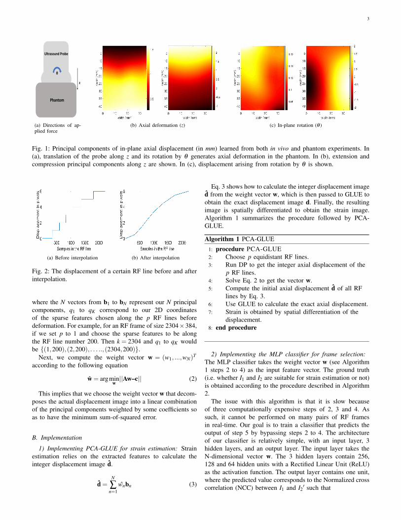
The idea is simple and logical: we compute N principalcomponents denoted by b1 to bN from real experiments thatdescribe TDE under the effect of an external force. In otherwords, the approximate displacement image is a linear combi-nation of these principal components. During data collection,we applied the force in the 6 degrees of freedom (DOF) toensure generality and a dataset of displacement images wasobtained using GLUE. Using PCA, we were able to computeour principal components. Fig. 1 shows the directions of theapplied force as well as some of the principal componentslearned.

For frame selection, our goal was simply to have a classifierthat can classify whether the two RF frames are suitable forstrain estimation. One can consider an approach of having aclassifier that takes the two RF frames, where the samplesare the input features (such as [18] and [20]), and outputsa binary decision of 1 for suitable frames and 0 otherwise.This approach would need a powerful GPU as the numberof samples in each RF frame is approximately 1 million. Tosimplify the problem, we make use of our representation forthe displacement image by the principal components. We canthink of this as a dimensionality reduction method for thehuge number of features that we had, where the input featurevector can be simply the N-dimensional weight vector w,which represents the weight of each principal component in theinitial displacement image. Our low-dimensional weight vectorw is the input to a multi-layer perceptron (MLP) classifier thatwould output a binary number 1 or 0 depending on whetherthe two RF frames are suitable or not for strain estimation.

A. Feature extraction

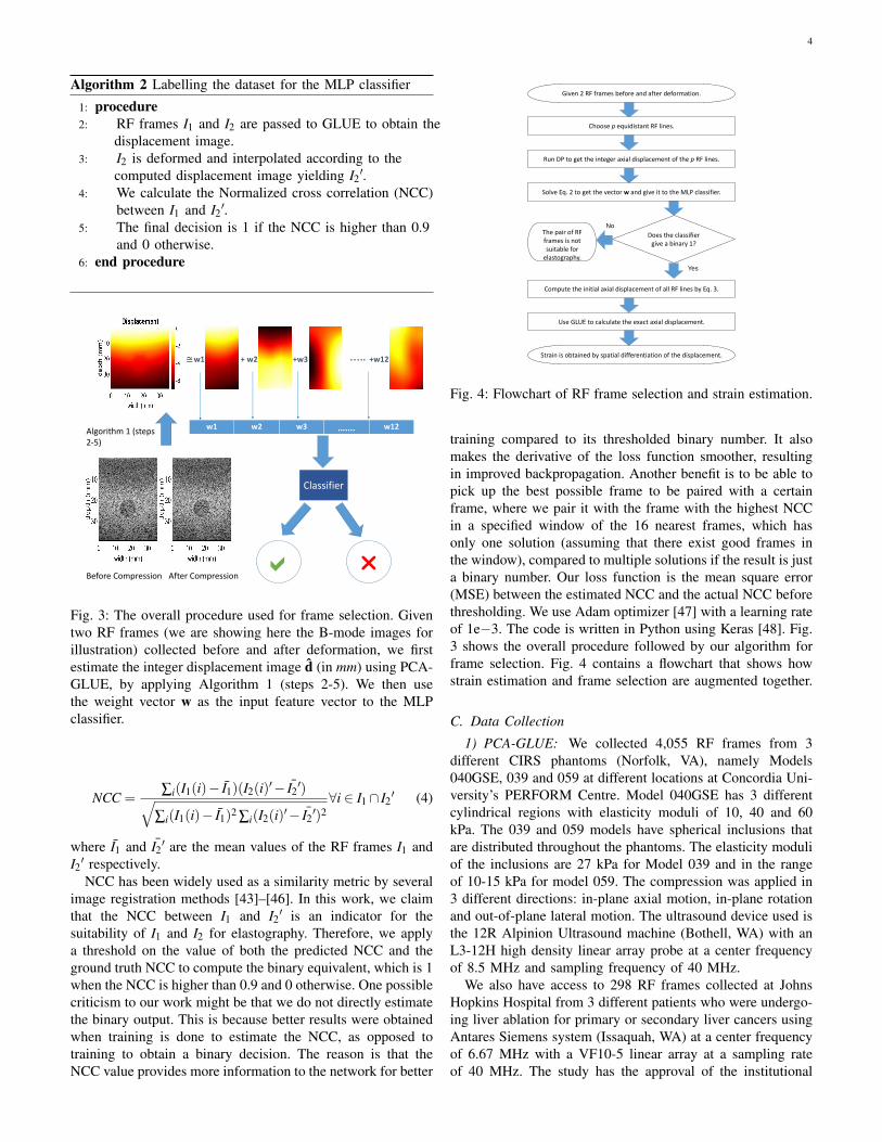
Consider having two RF frames I1 and I2 collected beforeand after some deformation, each of size m× l, where m is thenumber of samples in an RF-line and l is the number a RFlines. Our goal is to estimate a coarse displacement image thatdescribes the axial motion that each sample has had [42]. Westart by running the DP algorithm on only p RF lines out of thetotal l RF lines (where p << l) to get the integer displacementof k = m× p pixels. We then form a k-dimensional vectornamed c after applying a simple linear interpolation to the kestimates to make them smoother, so that the integer estimatesbecome linearly increasing with depth instead of the staircaseapproximation, as shown in Fig. 2.

Next, we construct the matrix A such that

A =

b1(q1) b2(q1) b3(q1) . . . bN(q1)b1(q2) b2(q2) b3(q2) . . . bN(q2). . . . . . . . . . . . . . . . . . . . . . . . . . . . . . . . . . . . . . . . .b1(qK) b2(qK) b3(qK) . . . bN(qK)

(1)

3

Ultrasound Probe

Phantom

θ

z

(a) Directions of ap-plied force

(b) Axial deformation (z) (c) In-plane rotation (θ )

Fig. 1: Principal components of in-plane axial displacement (in mm) learned from both in vivo and phantom experiments. In(a), translation of the probe along z and its rotation by θ generates axial deformation in the phantom. In (b), extension andcompression principal components along z are shown. In (c), displacement arising from rotation by θ is shown.

(a) Before interpolation (b) After interpolation

Fig. 2: The displacement of a certain RF line before and afterinterpolation.

where the N vectors from b1 to bN represent our N principalcomponents, q1 to qK correspond to our 2D coordinatesof the sparse features chosen along the p RF lines beforedeformation. For example, for an RF frame of size 2304×384,if we set p to 1 and choose the sparse features to be alongthe RF line number 200. Then k = 2304 and q1 to qK wouldbe {(1,200),(2,200), . . . ..,(2304,200)}.

Next, we compute the weight vector w = (w1, ...,wN)T

according to the following equation

w = argminw||Aw–c|| (2)

This implies that we choose the weight vector w that decom-poses the actual displacement image into a linear combinationof the principal components weighted by some coefficients soas to have the minimum sum-of-squared error.

B. Implementation

1) Implementing PCA-GLUE for strain estimation: Strainestimation relies on the extracted features to calculate theinteger displacement image d.

d =N

∑n=1

wnbn (3)

Eq. 3 shows how to calculate the integer displacement imaged from the weight vector w, which is then passed to GLUE toobtain the exact displacement image d. Finally, the resultingimage is spatially differentiated to obtain the strain image.Algorithm 1 summarizes the procedure followed by PCA-GLUE.

Algorithm 1 PCA-GLUE

1: procedure PCA-GLUE2: Choose p equidistant RF lines.3: Run DP to get the integer axial displacement of the

p RF lines.4: Solve Eq. 2 to get the vector w.5: Compute the initial axial displacement d of all RF

lines by Eq. 3.6: Use GLUE to calculate the exact axial displacement.7: Strain is obtained by spatial differentiation of the

displacement.8: end procedure

2) Implementing the MLP classifier for frame selection:The MLP classifier takes the weight vector w (see Algorithm1 steps 2 to 4) as the input feature vector. The ground truth(i.e. whether I1 and I2 are suitable for strain estimation or not)is obtained according to the procedure described in Algorithm2.

The issue with this algorithm is that it is slow becauseof three computationally expensive steps of 2, 3 and 4. Assuch, it cannot be performed on many pairs of RF framesin real-time. Our goal is to train a classifier that predicts theoutput of step 5 by bypassing steps 2 to 4. The architectureof our classifier is relatively simple, with an input layer, 3hidden layers, and an output layer. The input layer takes theN-dimensional vector w. The 3 hidden layers contain 256,128 and 64 hidden units with a Rectified Linear Unit (ReLU)as the activation function. The output layer contains one unit,where the predicted value corresponds to the Normalized crosscorrelation (NCC) between I1 and I2

′ such that

4

Algorithm 2 Labelling the dataset for the MLP classifier

1: procedure2: RF frames I1 and I2 are passed to GLUE to obtain the

displacement image.3: I2 is deformed and interpolated according to the

computed displacement image yielding I2′.

4: We calculate the Normalized cross correlation (NCC)between I1 and I2

′.5: The final decision is 1 if the NCC is higher than 0.9

and 0 otherwise.6: end procedure

≅w1 + w2 +w3 +w12…..

w1 w2 w3 ……. w12

Classifier

Algorithm 1 (steps2-5)

Before Compression After Compression

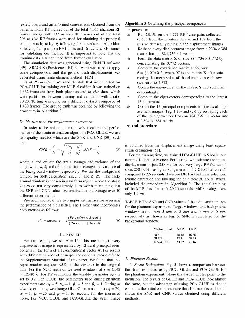
Fig. 3: The overall procedure used for frame selection. Giventwo RF frames (we are showing here the B-mode images forillustration) collected before and after deformation, we firstestimate the integer displacement image d (in mm) using PCA-GLUE, by applying Algorithm 1 (steps 2-5). We then usethe weight vector w as the input feature vector to the MLPclassifier.

NCC =∑i(I1(i)− I1)(I2(i)′− ¯I2

′)√∑i(I1(i)− I1)2 ∑i(I2(i)′− ¯I2

′)2∀i ∈ I1∩ I2

′ (4)

where I1 and ¯I2′ are the mean values of the RF frames I1 and

I2′ respectively.NCC has been widely used as a similarity metric by several

image registration methods [43]–[46]. In this work, we claimthat the NCC between I1 and I2

′ is an indicator for thesuitability of I1 and I2 for elastography. Therefore, we applya threshold on the value of both the predicted NCC and theground truth NCC to compute the binary equivalent, which is 1when the NCC is higher than 0.9 and 0 otherwise. One possiblecriticism to our work might be that we do not directly estimatethe binary output. This is because better results were obtainedwhen training is done to estimate the NCC, as opposed totraining to obtain a binary decision. The reason is that theNCC value provides more information to the network for better

Does the classifier give a binary 1?

Given 2 RF frames before and after deformation.

The pair of RF frames is not suitable for

elastography.

Yes

No

Use GLUE to calculate the exact axial displacement.

Compute the initial axial displacement of all RF lines by Eq. 3.

Solve Eq. 2 to get the vector w and give it to the MLP classifier.

Run DP to get the integer axial displacement of the p RF lines.

Choose p equidistant RF lines.

Strain is obtained by spatial differentiation of the displacement.

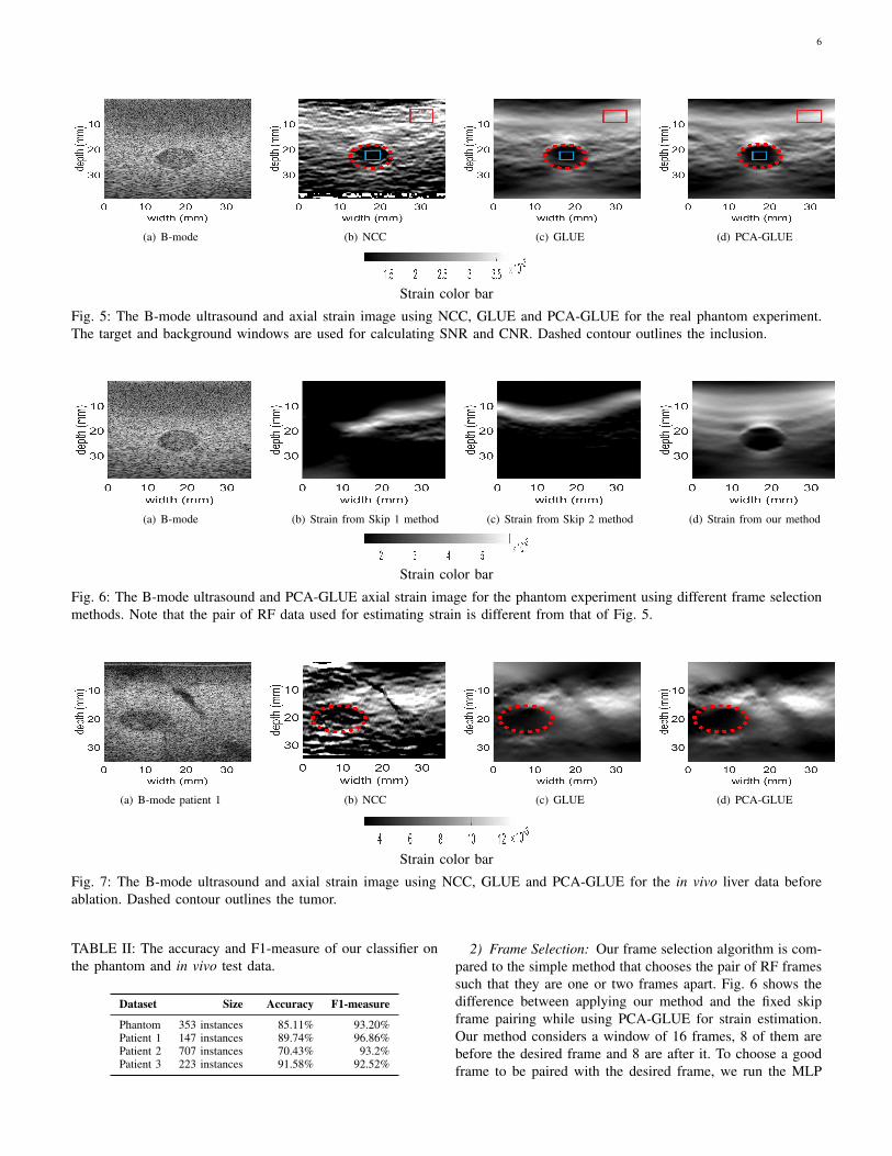
Fig. 4: Flowchart of RF frame selection and strain estimation.

training compared to its thresholded binary number. It alsomakes the derivative of the loss function smoother, resultingin improved backpropagation. Another benefit is to be able topick up the best possible frame to be paired with a certainframe, where we pair it with the frame with the highest NCCin a specified window of the 16 nearest frames, which hasonly one solution (assuming that there exist good frames inthe window), compared to multiple solutions if the result is justa binary number. Our loss function is the mean square error(MSE) between the estimated NCC and the actual NCC beforethresholding. We use Adam optimizer [47] with a learning rateof 1e−3. The code is written in Python using Keras [48]. Fig.3 shows the overall procedure followed by our algorithm forframe selection. Fig. 4 contains a flowchart that shows howstrain estimation and frame selection are augmented together.

C. Data Collection

1) PCA-GLUE: We collected 4,055 RF frames from 3different CIRS phantoms (Norfolk, VA), namely Models040GSE, 039 and 059 at different locations at Concordia Uni-versity’s PERFORM Centre. Model 040GSE has 3 differentcylindrical regions with elasticity moduli of 10, 40 and 60kPa. The 039 and 059 models have spherical inclusions thatare distributed throughout the phantoms. The elasticity moduliof the inclusions are 27 kPa for Model 039 and in the rangeof 10-15 kPa for model 059. The compression was applied in3 different directions: in-plane axial motion, in-plane rotationand out-of-plane lateral motion. The ultrasound device used isthe 12R Alpinion Ultrasound machine (Bothell, WA) with anL3-12H high density linear array probe at a center frequencyof 8.5 MHz and sampling frequency of 40 MHz.

We also have access to 298 RF frames collected at JohnsHopkins Hospital from 3 different patients who were undergo-ing liver ablation for primary or secondary liver cancers usingAntares Siemens system (Issaquah, WA) at a center frequencyof 6.67 MHz with a VF10-5 linear array at a sampling rateof 40 MHz. The study has the approval of the institutional

5

review board and an informed consent was obtained from thepatients. 3,635 RF frames out of the total 4,055 phantom RFframes, along with 137 in vivo RF frames out of the total298 in vivo RF frames were used for obtaining the principalcomponents b1 to bN by following the procedure in Algorithm3, leaving 420 phantom RF frames and 161 in vivo RF framesfor validating our method. It is important to note that thetraining data was excluded from further evaluation.

The simulation data was generated using Field II software[49]. ABAQUS (Providence, RI) software was used to applysome compression, and the ground truth displacement wasgenerated using finite element method (FEM).

2) MLP classifier: We used the data that we collected forPCA-GLUE for training our MLP classifier. It was trained on4,662 instances from both phantom and in vivo data, whichwere partitioned between training and validation with a ratio80:20. Testing was done on a different dataset composed of1,430 frames. The ground truth was obtained by following theprocedure in Algorithm 2.

D. Metrics used for performance assessment

In order to be able to quantitatively measure the perfor-mance of the strain estimation algorithm PCA-GLUE, we usetwo quality metrics which are the SNR and CNR [50], suchthat:

CNR =CN

=

√2(sb− st)2

σ2b +σ2

t,SNR =

sσ

(5)

where st and σ2t are the strain average and variance of the

target window, sb and σ2b are the strain average and variance of

the background window respectively. We use the backgroundwindow for SNR calculation (i.e. s=sb and σ=σb). The back-ground window is chosen in a uniform region where the strainvalues do not vary considerably. It is worth mentioning thatthe SNR and CNR values are obtained as the average over 10different experiments.

Precision and recall are two important metrics for assessingthe performance of a classifier. The F1-measure incorporatesboth metrics as follows:

F1−measure = 2(Precision×Recall)(Precision+Recall

(6)

III. RESULTS

For our results, we set N = 12. This means that everydisplacement image is represented by 12 axial principal com-ponents in the form of a 12-dimentional vector w. For resultswith different number of principal components, please refer tothe Supplementary Material of this paper. We found that thisrepresentation captures 95% of the variance in the originaldata. For the NCC method, we used windows of size (5.42× 12.49) λ . For DP estimation, the tunable parameter αDP isset to 0.2. For GLUE, the parameters used during phantomexperiments are α1 = 5, α2 = 1, β1 = 5 and β2 = 1. During invivo experiments, we change GLUE’s parameters to α1 = 20,α2 = 1, β1 = 20 and β2 = 1, to account for the increasednoise. For NCC, GLUE and PCA-GLUE, the strain image

Algorithm 3 Obtaining the principal components

1: procedure2: Run GLUE on the 3,772 RF frame pairs collected

(3,635 from the phantom dataset and 137 from thein vivo dataset), yielding 3,772 displacement images.

3: Reshape every displacement image from a 2304×384matrix into an 884,736×1 vector.

4: Form the data matrix X of size 884,736×3,772 byconcatenating the 3,772 vectors.

5: Compute the covariance matrix as follows:S = 1

n×X′×X′T , where X′ is the matrix X after subt-racting the mean value of the elements in each row(we set n to 3,772).

6: Obtain the eigenvalues of the matrix S and sort themdescendingly.

7: Compute the eigenvectors corresponding to the largest12 eigenvalues.

8: Obtain the 12 principal components for the axial displ-acement images (Fig. 1 (b) and (c)) by reshaping eachof the 12 eigenvectors from an 884,736×1 vector intoa 2,304 × 384 matrix.

9: end procedure

is obtained from the displacement image using least squarestrain estimation [51].

For the running time, we trained PCA-GLUE in 5 hours, buttraining is done only once. For testing, we estimate the initialdisplacement in just 258 ms for two very large RF frames ofsizes 2304×384 using an 8th generation 3.2 GHz Intel core i7compared to 2.6 seconds if we use DP. For the frame selection,feature extraction and labeling the data took 30 hours, whichincluded the procedure in Algorithm 2. The actual trainingof the MLP classifier took 29.16 seconds, while testing takesonly 1.5 ms.

TABLE I: The SNR and CNR values of the axial strain imagesfor the phantom experiment. Target windows and backgroundwindows are of size 3 mm × 3 mm and 5 mm × 5 mmrespectively as shown in Fig. 5. SNR is calculated for thebackground window.

Method used SNR CNR

NCC 18.18 16.86GLUE 22.31 20.65PCA-GLUE 23.52 21.46

A. Phantom Results

1) Strain Estimation: Fig. 5 shows a comparison betweenthe strain estimated using NCC, GLUE and PCA-GLUE forthe phantom experiment, where the dashed circles point to theinclusion. The results of GLUE and PCA-GLUE look almostthe same, but the advantage of using PCA-GLUE is that itestimates the initial estimates more than 10 times faster. Table Ishows the SNR and CNR values obtained using differentmethods.

6

(a) B-mode (b) NCC (c) GLUE (d) PCA-GLUE

Strain color bar

Fig. 5: The B-mode ultrasound and axial strain image using NCC, GLUE and PCA-GLUE for the real phantom experiment.The target and background windows are used for calculating SNR and CNR. Dashed contour outlines the inclusion.

(a) B-mode (b) Strain from Skip 1 method (c) Strain from Skip 2 method (d) Strain from our method

Strain color bar

Fig. 6: The B-mode ultrasound and PCA-GLUE axial strain image for the phantom experiment using different frame selectionmethods. Note that the pair of RF data used for estimating strain is different from that of Fig. 5.

(a) B-mode patient 1 (b) NCC (c) GLUE (d) PCA-GLUE

Strain color bar

Fig. 7: The B-mode ultrasound and axial strain image using NCC, GLUE and PCA-GLUE for the in vivo liver data beforeablation. Dashed contour outlines the tumor.

TABLE II: The accuracy and F1-measure of our classifier onthe phantom and in vivo test data.

Dataset Size Accuracy F1-measure

Phantom 353 instances 85.11% 93.20%Patient 1 147 instances 89.74% 96.86%Patient 2 707 instances 70.43% 93.2%Patient 3 223 instances 91.58% 92.52%

2) Frame Selection: Our frame selection algorithm is com-pared to the simple method that chooses the pair of RF framessuch that they are one or two frames apart. Fig. 6 shows thedifference between applying our method and the fixed skipframe pairing while using PCA-GLUE for strain estimation.Our method considers a window of 16 frames, 8 of them arebefore the desired frame and 8 are after it. To choose a goodframe to be paired with the desired frame, we run the MLP

7

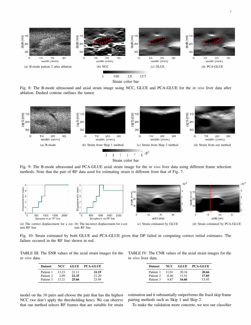
(a) B-mode patient 2 after ablation (b) NCC (c) GLUE (d) PCA-GLUE

Strain color bar

Fig. 8: The B-mode ultrasound and axial strain image using NCC, GLUE and PCA-GLUE for the in vivo liver data afterablation. Dashed contour outlines the tumor.

(a) B-mode (b) Strain from Skip 1 method (c) Strain from Skip 2 method (d) Strain from our method

Strain color bar

Fig. 9: The B-mode ultrasound and PCA-GLUE axial strain image for the in vivo liver data using different frame selectionmethods. Note that the pair of RF data used for estimating strain is different from that of Fig. 7.

(a) The correct displacement for a cer-tain RF line

(b) The incorrect displacement for a cer-tain RF line

(c) Strain estimated by GLUE (d) Strain estimated by PCA-GLUE

Fig. 10: Strain estimated by both GLUE and PCA-GLUE given that DP failed in computing correct initial estimates. Thefailure occured in the RF line shown in red.

TABLE III: The SNR values of the axial strain images for thein vivo data.

Dataset NCC GLUE PCA-GLUE

Patient 1 13.23 21.11 21.19Patient 2 2.09 21.33 21.20Patient 3 13.21 25.66 23.94

model on the 16 pairs and choose the pair that has the highestNCC (we don’t apply the thresholding here). We can observethat our method selects RF frames that are suitable for strain

TABLE IV: The CNR values of the axial strain images for thein vivo liver data.

Dataset NCC GLUE PCA-GLUE

Patient 1 11.01 20.34 20.66Patient 2 -0.46 13.52 17.05Patient 3 9.87 16.66 15.95

estimation and it substantially outperforms the fixed skip framepairing methods such as Skip 1 and Skip 2.

To make the validation more concrete, we test our classifier

8

on 353 instances to classify them as suitable or not suitable forstrain estimation. The ground truth is obtained as previouslydiscussed in Algorithm 2. Table II shows the accuracy andF1-measure for our classifier on new data that the model hasnot seen before. The results show that our classifier is able togeneralize well to unseen data, and that it could be used inpractice.

B. In vivo Results

1) Strain Estimation: Fig. 7 and 8 show the results obtainedwhen running NCC, GLUE and PCA-GLUE on the liverdataset, where both GLUE and PCA-GLUE yield very similarresults. The dashed ellipses point to the tumors. Tables IIIand IV show the SNR and CNR calculated.

2) Frame Selection: Fig. 9 shows a comparison betweenthe strain estimated using both our frame selection methodand the fixed skip frame pairing on two RF frames collectedfrom the in vivo liver data. Table II shows the accuracy andF1-measure obtained for the liver dataset.

C. PCA-GLUE robustness

Our method is not only capable of estimating strain orselecting suitable RF frames, it is also robust to incorrect initialdisplacement estimates when DP fails. The main differencebetween PCA-GLUE and GLUE is in estimating the initialdisplacement image, where GLUE uses DP to estimate thedisplacement of every single RF line, whereas PCA-GLUEapplies DP for only 5 RF lines, then uses a linear combinationof previously computed principal components as an initialdisplacement image. Therefore, if DP fails in estimating thecorrect displacement for a certain RF line, that means thatGLUE would have an incorrect initial displacement image,which affects the fine-tuned displacement image.

The reason behind this robustness is that PCA-GLUE relieson the principal components previously computed offline, suchthat the resulting initial displacement image is represented as alinear combination of them. Therefore, if incorrect results wereamong the 5 RF lines chosen by PCA-GLUE, it would stillbe able to estimate the strain correctly due to the additionalstep of estimating TDE as a sum of principal components.

Fig. 10 shows how both GLUE and PCA-GLUE performwhen they get incorrect initial estimates from DP.

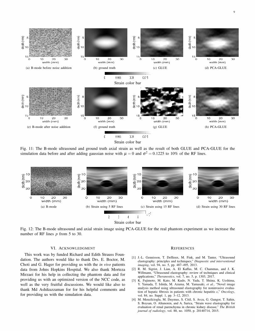
Fig. 11 shows a comparison between the strain estimatedby both GLUE and PCA-GLUE on the finite element method(FEM) simulation data before and after adding a gaussiannoise with µ = 0 and σ2 = 0.1225 to 10% of the RF lines. Thelarge error on these RF lines could be caused in real life due toair bubbles between the probe and tissue, or large out-of-planemotion in some regions.

D. Varying the number of sparse features

Fig. 12 shows the effect of running DP on more than 5RF lines. We can conclude that the accuracy of the strainestimation does not improve any further when setting p toa value more than 5. As more RF lines correspond to morefeatures and consequently more computations, we choose the

smallest value p= 5 without sacrificing the accuracy. For moreanalysis and results at different values of p, please refer to theSupplementary Material of the paper.

IV. DISCUSSION

We presented a novel method that can estimate a coarsedisplacement map from a sparse set of displacement dataprovided by DP. For an image of size 2304×384, DP takes163 ms and estimation of coarse displacement field takes 95ms, for a total of 258 ms. We also presented a novel methodfor frame selection that classifies a pair of RF Data as suitableor unsuitable for elastography in only 1.5 ms. The input toour classifier is the w vector and not the RF data or thedisplacement image. The reason is that inference with suchlow-dimensional input is very computationally efficient.

During training, we tried using datasets with and withoutinclusions to obtain the principal components. Our conclusionis that the presence or absence of inclusions in the trainingdata does not alter the principal components and consequentlythe strain estimated. What is critical for learning the principalcomponents is the presence of different types of deformation,such as axial, lateral and rotational deformation.

It is worth mentioning that we were only concerned withthe axial displacement, as we couldn’t compute any principalcomponents that describe the lateral displacement. The reasonis that by following Algorithm 3 for the lateral displacement,we found that the variance is not concentrated in the first feweigenvectors, unlike the axial displacement. It is rather almostequally distributed over hundreds of eigenvectors (resemblingwhite noise). We conclude that capturing 95% of the variancewould require us to save hundreds of principal components,which is not practical. Therefore, we only use the integerestimates for the k = m× p pixels computed by DP, followedby bi-linear interpolation which provides an acceptable initiallateral displacement, compared to the alternative approachwhere we run DP on all RF lines. A comparison between thelateral displacement estimated by the two approaches is shownin the Supplementary Material. The combination of N = 12and p = 5 is not a fixed choice of the hyperparameters, asdifferent datasets would require different tuning. In our case,this choice is adequate for all the datasets used.

V. CONCLUSION

In this paper, we introduced a new method with two maincontributions which are fast strain estimation and RF frameselection. In addition, our method is robust to incorrect initialestimates by DP. Our method is more than 10 times fasterthan GLUE in estimating the initial displacement image, whichis the step prior to the exact displacement estimation, whilegiving the same or better results. Our MLP classifier usedfor frame selection has been tested on 1,430 unseen pairsof RF frames from both phantom and in vivo datasets, andthe F1-measure obtained was always higher than 92%. Thisproves that our method is efficient and that it could be usedcommercially.

9

(a) B-mode before noise addition (b) ground truth (c) GLUE (d) PCA-GLUE

Strain color bar

(e) B-mode after noise addition (f) ground truth (g) GLUE (h) PCA-GLUE

Strain color bar

Fig. 11: The B-mode ultrasound and ground truth axial strain as well as the result of both GLUE and PCA-GLUE for thesimulation data before and after adding gaussian noise with µ = 0 and σ2 = 0.1225 to 10% of the RF lines.

(a) B-mode (b) Strain using 5 RF lines (c) Strain using 15 RF lines (d) Strain using 30 RF lines

Strain color bar

Fig. 12: The B-mode ultrasound and axial strain image using PCA-GLUE for the real phantom experiment as we increase thenumber of RF lines p from 5 to 30.

VI. ACKNOWLEDGMENT

This work was by funded Richard and Edith Strauss Foun-dation. The authors would like to thank Drs. E. Boctor, M.Choti and G. Hager for providing us with the in vivo patientsdata from Johns Hopkins Hospital. We also thank MortezaMirzaei for his help in collecting the phantom data and forproviding us with an optimized version of the NCC code, aswell as the very fruitful discussions. We would like also tothank Md Ashikuzzaman for for his helpful comments andfor providing us with the simulation data.

REFERENCES

[1] J.-L. Gennisson, T. Deffieux, M. Fink, and M. Tanter, “Ultrasoundelastography: principles and techniques,” Diagnostic and interventionalimaging, vol. 94, no. 5, pp. 487–495, 2013.

[2] R. M. Sigrist, J. Liau, A. El Kaffas, M. C. Chammas, and J. K.Willmann, “Ultrasound elastography: review of techniques and clinicalapplications,” Theranostics, vol. 7, no. 5, p. 1303, 2017.

[3] K. Fujimoto, M. Kato, M. Kudo, N. Yada, T. Shiina, K. Ueshima,Y. Yamada, T. Ishida, M. Azuma, M. Yamasaki, et al., “Novel imageanalysis method using ultrasound elastography for noninvasive evalua-tion of hepatic fibrosis in patients with chronic hepatitis c,” Oncology,vol. 84, no. Suppl. 1, pp. 3–12, 2013.

[4] M. Menzilcioglu, M. Duymus, S. Citil, S. Avcu, G. Gungor, T. Sahin,S. Boysan, O. Altunoren, and A. Sarica, “Strain wave elastography forevaluation of renal parenchyma in chronic kidney disease,” The Britishjournal of radiology, vol. 88, no. 1050, p. 20140714, 2015.

10

[5] R. G. Barr, K. Nakashima, D. Amy, D. Cosgrove, A. Farrokh, F. Schafer,J. C. Bamber, L. Castera, B. I. Choi, Y.-H. Chou, et al., “Wfumb guide-lines and recommendations for clinical use of ultrasound elastography:Part 2: breast,” Ultrasound in medicine & biology, vol. 41, no. 5, pp.1148–1160, 2015.

[6] M. Brock, C. von Bodman, R. J. Palisaar, B. Loppenberg, F. Sommerer,T. Deix, J. Noldus, and T. Eggert, “The impact of real-time elastographyguiding a systematic prostate biopsy to improve cancer detection rate:a prospective study of 353 patients,” The Journal of urology, vol. 187,no. 6, pp. 2039–2043, 2012.

[7] J. Bojunga, E. Herrmann, G. Meyer, S. Weber, S. Zeuzem, andM. Friedrich-Rust, “Real-time elastography for the differentiation ofbenign and malignant thyroid nodules: a meta-analysis,” Thyroid, vol. 20,no. 10, pp. 1145–1150, 2010.

[8] G. Ferraioli, C. Filice, L. Castera, B. I. Choi, I. Sporea, S. R. Wilson,D. Cosgrove, C. F. Dietrich, D. Amy, J. C. Bamber, et al., “Wfumbguidelines and recommendations for clinical use of ultrasound elastog-raphy: Part 3: liver,” Ultrasound in medicine & biology, vol. 41, no. 5,pp. 1161–1179, 2015.

[9] T. J Hall, P. E Barboneg, A. A Oberai, J. Jiang, J.-F. Dord, S. Goenezen,and T. G Fisher, “Recent results in nonlinear strain and modulusimaging,” Current medical imaging reviews, vol. 7, no. 4, pp. 313–327,2011.

[10] K. Parker, M. Doyley, and D. Rubens, “Imaging the elastic properties oftissue: the 20 year perspective,” Physics in medicine & biology, vol. 56,no. 1, p. R1, 2010.

[11] J. Ophir, I. Cespedes, H. Ponnekanti, Y. Yazdi, and X. Li, “Elastography:a quantitative method for imaging the elasticity of biological tissues,”Ultrasonic imaging, vol. 13, no. 2, pp. 111–134, 1991.

[12] Q. He, L. Tong, L. Huang, J. Liu, Y. Chen, and J. Luo, “Performanceoptimization of lateral displacement estimation with spatial angularcompounding,” Ultrasonics, vol. 73, pp. 9–21, 2017.

[13] Y. Wang, M. Bayer, J. Jiang, and T. J. Hall, “Large-strain 3-d in vivobreast ultrasound strain elastography using a multi-compression strategyand a whole-breast scanning system,” Ultrasound in medicine & biology,vol. 45, no. 12, pp. 3145–3159, 2019.

[14] R. M. Pohlman and T. Varghese, “Physiological motion reduction usinglagrangian tracking for electrode displacement elastography,” Ultrasoundin Medicine & Biology, 2019.

[15] G.-Y. Li, Q. He, G. Xu, L. Jia, J. Luo, and Y. Cao, “An ultrasoundelastography method to determine the local stiffness of arteries withguided circumferential waves,” Journal of biomechanics, vol. 51, pp.97–104, 2017.

[16] S. Wu, Z. Gao, Z. Liu, J. Luo, H. Zhang, and S. Li, “Direct recon-struction of ultrasound elastography using an end-to-end deep neuralnetwork,” in International Conference on Medical Image Computingand Computer-Assisted Intervention. Springer, 2018, pp. 374–382.

[17] C. Hoerig, J. Ghaboussi, and M. F. Insana, “Data-driven elasticityimaging using cartesian neural network constitutive models and the au-toprogressive method,” IEEE transactions on medical imaging, vol. 38,no. 5, pp. 1150–1160, 2018.

[18] B. Peng, Y. Xian, and J. Jiang, “A convolution neural network-basedspeckle tracking method for ultrasound elastography,” in 2018 IEEEInternational Ultrasonics Symposium (IUS). IEEE, 2018, pp. 206–212.

[19] Z. Gao, S. Wu, Z. Liu, J. Luo, H. Zhang, M. Gong, and S. Li,“Learning the implicit strain reconstruction in ultrasound elastographyusing privileged information,” Medical image analysis, vol. 58, p.101534, 2019.

[20] M. G. Kibria and H. Rivaz, “Gluenet: Ultrasound elastography usingconvolutional neural network,” in Simulation, Image Processing, andUltrasound Systems for Assisted Diagnosis and Navigation. Springer,2018, pp. 21–28.

[21] B. Peng, Y. Xian, Q. Zhang, and J. Jiang, “Neural network-basedmotion tracking for breast ultrasound strain elastography: An initialassessment of performance and feasibility,” Ultrasonic Imaging, p.0161734620902527, 2020.

[22] A. K. Tehrani and H. Rivaz, “Displacement estimation in ultrasoundelastography using pyramidal convolutional neural network,” IEEETransactions on Ultrasonics, Ferroelectrics, and Frequency Control,2020.

[23] D. Sun, X. Yang, M.-Y. Liu, and J. Kautz, “Pwc-net: Cnns for opticalflow using pyramid, warping, and cost volume,” in Proceedings of theIEEE Conference on Computer Vision and Pattern Recognition, 2018,pp. 8934–8943.

[24] H. S. Hashemi and H. Rivaz, “Global time-delay estimation in ultrasoundelastography,” IEEE transactions on ultrasonics, ferroelectrics, andfrequency control, vol. 64, no. 10, pp. 1625–1636, 2017.

[25] H. Rivaz, E. M. Boctor, M. A. Choti, and G. D. Hager, “Real-timeregularized ultrasound elastography,” IEEE transactions on medicalimaging, vol. 30, no. 4, pp. 928–945, 2011.

[26] M. Ashikuzzaman, C. J. Gauthier, and H. Rivaz, “Global ultrasoundelastography in spatial and temporal domains,” IEEE transactions onultrasonics, ferroelectrics, and frequency control, vol. 66, no. 5, pp.876–887, 2019.

[27] J. Jiang and T. J. Hall, “A coupled subsample displacement estimationmethod for ultrasound-based strain elastography,” Physics in Medicine& Biology, vol. 60, no. 21, p. 8347, 2015.

[28] L. Yuan and P. C. Pedersen, “Analytical phase-tracking-based strainestimation for ultrasound elasticity,” IEEE transactions on ultrasonics,ferroelectrics, and frequency control, vol. 62, no. 1, pp. 185–207, 2015.

[29] J. Luo and E. E. Konofagou, “A fast normalized cross-correlation calcu-lation method for motion estimation,” IEEE transactions on ultrasonics,ferroelectrics, and frequency control, vol. 57, no. 6, pp. 1347–1357,2010.

[30] J. Wulff and M. J. Black, “Efficient sparse-to-dense optical flow esti-mation using a learned basis and layers,” in IEEE Conf. on ComputerVision and Pattern Recognition (CVPR) 2015, June 2015.

[31] R. M. Pohlman and T. Varghese, “Dictionary representations for elec-trode displacement elastography,” IEEE transactions on ultrasonics,ferroelectrics, and frequency control, vol. 65, no. 12, pp. 2381–2389,2018.

[32] T. J. Hall, Y. Zhu, and C. S. Spalding, “In vivo real-time freehandpalpation imaging,” Ultrasound in medicine & biology, vol. 29, no. 3,pp. 427–435, 2003.

[33] R. Chandrasekhar, J. Ophir, T. Krouskop, and K. Ophir, “Elastographicimage quality vs. tissue motion in vivo,” Ultrasound in medicine &biology, vol. 32, no. 6, pp. 847–855, 2006.

[34] M. A. Lubinski, S. Y. Emelianov, and M. O’Donnell, “Adaptive strainestimation using retrospective processing [medical us elasticity imag-ing],” IEEE transactions on ultrasonics, ferroelectrics, and frequencycontrol, vol. 46, no. 1, pp. 97–107, 1999.

[35] K. M. Hiltawsky, M. Kruger, C. Starke, L. Heuser, H. Ermert, andA. Jensen, “Freehand ultrasound elastography of breast lesions: clinicalresults,” Ultrasound in medicine & biology, vol. 27, no. 11, pp. 1461–1469, 2001.

[36] J. Jiang, T. J. Hall, and A. M. Sommer, “A novel performance descriptorfor ultrasonic strain imaging: A preliminary study,” IEEE transactionson ultrasonics, ferroelectrics, and frequency control, vol. 53, no. 6, pp.1088–1102, 2006.

[37] H. Rivaz, P. Foroughi, I. Fleming, R. Zellars, E. Boctor, and G. Hager,“Tracked regularized ultrasound elastography for targeting breast radio-therapy,” in International Conference on Medical Image Computing andComputer-Assisted Intervention. Springer, 2009, pp. 507–515.

[38] P. Foroughi, H.-J. Kang, D. A. Carnegie, M. G. van Vledder, M. A.Choti, G. D. Hager, and E. M. Boctor, “A freehand ultrasound elas-tography system with tracking for in vivo applications,” Ultrasound inmedicine & biology, vol. 39, no. 2, pp. 211–225, 2013.

[39] A. Zayed and H. Rivaz, “Fast approximate time-delay estimation inultrasound elastography using principal component analysis,” in 201941st Annual International Conference of the IEEE Engineering inMedicine and Biology Society (EMBC). IEEE, 2019, pp. 6204–6207.

[40] A. Zayed and H. Rivaz, “Automatic frame selection using mlp neuralnetwork in ultrasound elastography,” in International Conference onImage Analysis and Recognition. Springer, 2019, pp. 462–472.

[41] H. Rivaz, E. Boctor, P. Foroughi, R. Zellars, G. Fichtinger, and G. Hager,“Ultrasound elastography: a dynamic programming approach,” IEEEtransactions on medical imaging, vol. 27, no. 10, pp. 1373–1377, 2008.

[42] B. S. Garra, “Elastography: history, principles, and technique compari-son,” Abdominal imaging, vol. 40, no. 4, pp. 680–697, 2015.

[43] B. D. de Vos, F. F. Berendsen, M. A. Viergever, M. Staring, and I. Isgum,“End-to-end unsupervised deformable image registration with a convo-lutional neural network,” in Deep Learning in Medical Image Analysisand Multimodal Learning for Clinical Decision Support. Springer,2017, pp. 204–212.

[44] S. Chicotay, E. David, and N. S. Netanyahu, “A two-phase geneticalgorithm for image registration,” in Proceedings of the Genetic andEvolutionary Computation Conference Companion, 2017, pp. 189–190.

[45] H. Li and Y. Fan, “Non-rigid image registration using self-supervisedfully convolutional networks without training data,” in 2018 IEEE 15thInternational Symposium on Biomedical Imaging (ISBI 2018). IEEE,2018, pp. 1075–1078.

[46] A. Subramaniam, P. Balasubramanian, and A. Mittal, “Ncc-net: Nor-malized cross correlation based deep matcher with robustness to illumi-

11

nation variations,” in 2018 IEEE Winter Conference on Applications ofComputer Vision (WACV). IEEE, 2018, pp. 1944–1953.

[47] D. P. Kingma and J. Ba, “Adam: A method for stochastic optimization,”arXiv preprint arXiv:1412.6980, 2014.

[48] F. Chollet et al., “Keras,” 2015.[49] J. A. Jensen, “Field: A program for simulating ultrasound systems,” in

10th Nordic-Baltic Conference on Biomedical Imaging, Vol. 4, Supple-ment 1, Part 1: 351–353, 1996.

[50] J. Ophir, S. K. Alam, B. Garra, F. Kallel, E. Konofagou, T. Krouskop,and T. Varghese, “Elastography: ultrasonic estimation and imaging ofthe elastic properties of tissues,” Proceedings Inst. Mech. Eng., Part H:J. Eng. in Med., vol. 213, no. 3, pp. 203–233, 1999.

[51] F. Kallel and J. Ophir, “A least-squares strain estimator for elastography,”Ultrasonic imaging, vol. 19, no. 3, pp. 195–208, 1997.

1

Fast Strain Estimation and Frame Selection inUltrasound Elastography using Machine Learning

Abdelrahman Zayed, Student Member, IEEE and Hassan Rivaz, Senior Member, IEEE

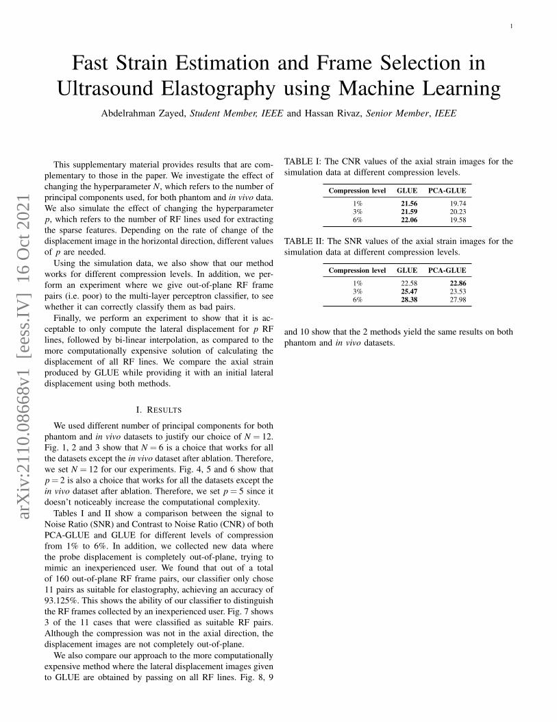
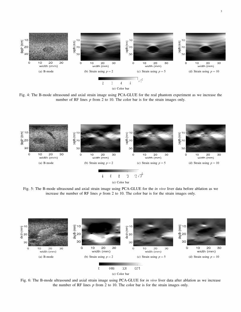
This supplementary material provides results that are com-plementary to those in the paper. We investigate the effect ofchanging the hyperparameter N, which refers to the number ofprincipal components used, for both phantom and in vivo data.We also simulate the effect of changing the hyperparameterp, which refers to the number of RF lines used for extractingthe sparse features. Depending on the rate of change of thedisplacement image in the horizontal direction, different valuesof p are needed.

Using the simulation data, we also show that our methodworks for different compression levels. In addition, we per-form an experiment where we give out-of-plane RF framepairs (i.e. poor) to the multi-layer perceptron classifier, to seewhether it can correctly classify them as bad pairs.

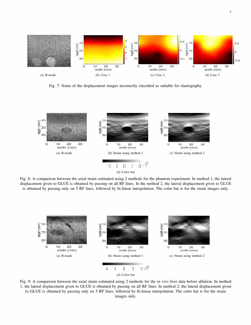
Finally, we perform an experiment to show that it is ac-ceptable to only compute the lateral displacement for p RFlines, followed by bi-linear interpolation, as compared to themore computationally expensive solution of calculating thedisplacement of all RF lines. We compare the axial strainproduced by GLUE while providing it with an initial lateraldisplacement using both methods.

I. RESULTS

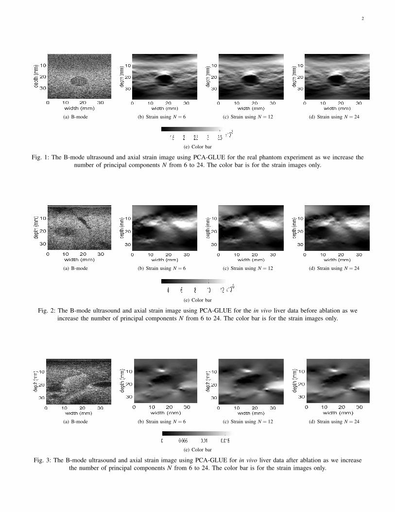
We used different number of principal components for bothphantom and in vivo datasets to justify our choice of N = 12.Fig. 1, 2 and 3 show that N = 6 is a choice that works for allthe datasets except the in vivo dataset after ablation. Therefore,we set N = 12 for our experiments. Fig. 4, 5 and 6 show thatp = 2 is also a choice that works for all the datasets except thein vivo dataset after ablation. Therefore, we set p = 5 since itdoesn’t noticeably increase the computational complexity.

Tables I and II show a comparison between the signal toNoise Ratio (SNR) and Contrast to Noise Ratio (CNR) of bothPCA-GLUE and GLUE for different levels of compressionfrom 1% to 6%. In addition, we collected new data wherethe probe displacement is completely out-of-plane, trying tomimic an inexperienced user. We found that out of a totalof 160 out-of-plane RF frame pairs, our classifier only chose11 pairs as suitable for elastography, achieving an accuracy of93.125%. This shows the ability of our classifier to distinguishthe RF frames collected by an inexperienced user. Fig. 7 shows3 of the 11 cases that were classified as suitable RF pairs.Although the compression was not in the axial direction, thedisplacement images are not completely out-of-plane.

We also compare our approach to the more computationallyexpensive method where the lateral displacement images givento GLUE are obtained by passing on all RF lines. Fig. 8, 9

TABLE I: The CNR values of the axial strain images for thesimulation data at different compression levels.

Compression level GLUE PCA-GLUE

1% 21.56 19.743% 21.59 20.236% 22.06 19.58

TABLE II: The SNR values of the axial strain images for thesimulation data at different compression levels.

Compression level GLUE PCA-GLUE

1% 22.58 22.863% 25.47 23.536% 28.38 27.98

and 10 show that the 2 methods yield the same results on bothphantom and in vivo datasets.

arX

iv:2

110.

0866

8v1

[ee

ss.I

V]

16

Oct

202

1

2

(a) B-mode (b) Strain using N = 6 (c) Strain using N = 12 (d) Strain using N = 24

(e) Color bar

Fig. 1: The B-mode ultrasound and axial strain image using PCA-GLUE for the real phantom experiment as we increase thenumber of principal components N from 6 to 24. The color bar is for the strain images only.

(a) B-mode (b) Strain using N = 6 (c) Strain using N = 12 (d) Strain using N = 24

(e) Color bar

Fig. 2: The B-mode ultrasound and axial strain image using PCA-GLUE for the in vivo liver data before ablation as weincrease the number of principal components N from 6 to 24. The color bar is for the strain images only.

(a) B-mode (b) Strain using N = 6 (c) Strain using N = 12 (d) Strain using N = 24

(e) Color bar

Fig. 3: The B-mode ultrasound and axial strain image using PCA-GLUE for in vivo liver data after ablation as we increasethe number of principal components N from 6 to 24. The color bar is for the strain images only.

3

(a) B-mode (b) Strain using p = 2 (c) Strain using p = 5 (d) Strain using p = 10

(e) Color bar

Fig. 4: The B-mode ultrasound and axial strain image using PCA-GLUE for the real phantom experiment as we increase thenumber of RF lines p from 2 to 10. The color bar is for the strain images only.

(a) B-mode (b) Strain using p = 2 (c) Strain using p = 5 (d) Strain using p = 10

(e) Color bar

Fig. 5: The B-mode ultrasound and axial strain image using PCA-GLUE for the in vivo liver data before ablation as weincrease the number of RF lines p from 2 to 10. The color bar is for the strain images only.

(a) B-mode (b) Strain using p = 2 (c) Strain using p = 5 (d) Strain using p = 10

(e) Color bar

Fig. 6: The B-mode ultrasound and axial strain image using PCA-GLUE for in vivo liver data after ablation as we increasethe number of RF lines p from 2 to 10. The color bar is for the strain images only.

4

(a) B-mode (b) Case 1 (c) Case 2 (d) Case 3

Fig. 7: Some of the displacement images incorrectly classified as suitable for elastography.

(a) B-mode (b) Strain using method 1 (c) Strain using method 2

(d) Color bar

Fig. 8: A comparison between the axial strain estimated using 2 methods for the phantom experiment. In method 1, the lateraldisplacement given to GLUE is obtained by passing on all RF lines. In the method 2, the lateral displacement given to GLUE

is obtained by passing only on 5 RF lines, followed by bi-linear interpolation. The color bar is for the strain images only.

(a) B-mode (b) Strain using method 1 (c) Strain using method 2

(d) Color bar

Fig. 9: A comparison between the axial strain estimated using 2 methods for the in vivo liver data before ablation. In method1, the lateral displacement given to GLUE is obtained by passing on all RF lines. In method 2, the lateral displacement given

to GLUE is obtained by passing only on 5 RF lines, followed by bi-linear interpolation. The color bar is for the strainimages only.

5

(a) B-mode (b) Strain using method 1 (c) Strain using method 2

(d) Color bar

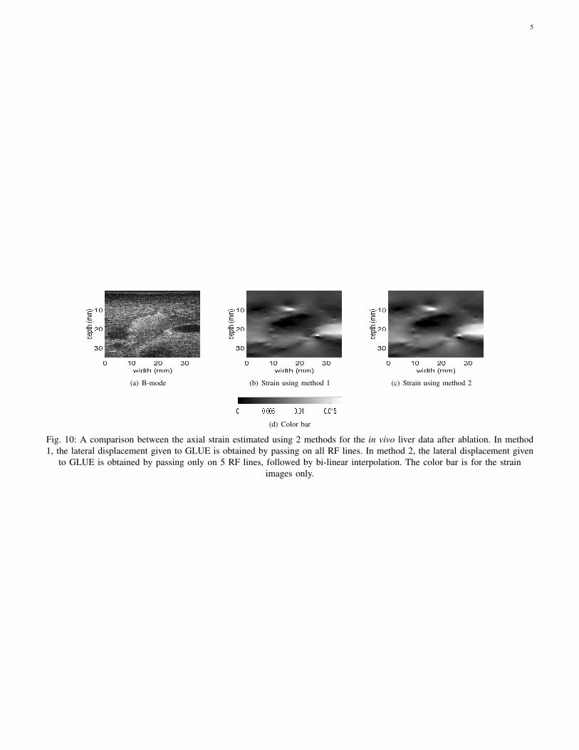
Fig. 10: A comparison between the axial strain estimated using 2 methods for the in vivo liver data after ablation. In method1, the lateral displacement given to GLUE is obtained by passing on all RF lines. In method 2, the lateral displacement given

to GLUE is obtained by passing only on 5 RF lines, followed by bi-linear interpolation. The color bar is for the strainimages only.