Please cite this article as: T. Weinhart, L. Orefice, M. Post et al., Fast, flexible particle simulations — An introduction to MercuryDPM, Computer Physics Communications (2019) 107129, https://doi.org/10.1016/j.cpc.2019.107129. Computer Physics Communications xxx (xxxx) xxx Contents lists available at ScienceDirect Computer Physics Communications journal homepage: www.elsevier.com/locate/cpc CPC 50th anniversary article Fast, flexible particle simulations — An introduction to MercuryDPM ✩, ✩✩ Thomas Weinhart a,b,∗ , Luca Orefice c,d , Mitchel Post a , Marnix P. van Schrojenstein Lantman a , Irana F.C. Denissen a , Deepak R. Tunuguntla a , J.M.F. Tsang e , Hongyang Cheng a , Mohamad Yousef Shaheen a , Hao Shi a,b , Paolo Rapino b , Elena Grannonio g , Nunzio Losacco g , Joao Barbosa h , Lu Jing f , Juan E. Alvarez Naranjo a , Sudeshna Roy a , Wouter K. den Otter a , Anthony R. Thornton a,b a Multiscale Mechanics, Engineering Technology, MESA+, University of Twente, PO Box 217, 7500 AE Enschede, The Netherlands b Mercury Lab BV, Mekkelholtsweg 10, 7523 DE Enschede, The Netherlands c Research Center Pharmaceutical Engineering (RCPE) GmbH, Inffeldgaße 13, 8010 Graz, Austria d European Consortium on Continuous Pharmaceutical Manufacturing (ECCPM), 8010 Graz, Austria e DAMTP, Centre for Mathematical Sciences, University of Cambridge, Wilberforce Road, Cambridge CB3 0WA, United Kingdom f Department of Chemical and Biological Engineering, Northwestern University, Evanston, IL 60208, USA g Department of Civil Engineering and Computer Science, University of Rome ‘‘Tor Vergata’’, Via del Politecnico 1, 00133 Rome, Italy h Department of Engineering Structures, Section of Dynamics of Solids and Structures, CiTG, TU Delft, Stevinweg 1, 2628 CN Delft, The Netherlands article info Article history: Received 12 August 2019 Received in revised form 29 November 2019 Accepted 2 December 2019 Available online xxxx Keywords: Granular materials DEM DPM MercuryDPM Open-source abstract We introduce the open-source package MercuryDPM, which we have been developing over the last few years. MercuryDPM is a code for discrete particle simulations. It simulates the motion of particles by applying forces and torques that stem either from external body forces, (gravity, magnetic fields, etc.) or particle interactions. The code has been developed extensively for granular applications, and in this case these are typically (elastic, plastic, viscous, frictional) contact forces or (adhesive) short-range forces. However, it could be adapted to include long-range (molecular, self-gravity) interactions as well. MercuryDPM is an object-oriented algorithm with an easy-to-use user interface and a flexible core, allowing developers to quickly add new features. It is parallelised using MPI and released under the BSD 3-clause licence. Its open-source developers’ community has developed many features, including moving and curved walls; state-of-the-art granular contact models; specialised classes for common geometries; non-spherical particles; general interfaces; restarting; visualisation; a large self-test suite; extensive documentation; and numerous tutorials and demos. In addition, MercuryDPM has three major components that were originally invented and developed by its team: an advanced contact detection method, which allows for the first time large simulations with wide size distributions; curved (non- triangulated) walls; and multicomponent, spatial and temporal coarse-graining, a novel way to extract continuum fields from discrete particle systems. We illustrate these tools and a selection of other MercuryDPM features via various applications, including size-driven segregation down inclined planes, rotating drums, and dosing silos. Program summary Program Title: MercuryDPM Program Files doi: http://dx.doi.org/10.17632/n7jmdrdc52.1 Licensing provisions: BSD 3-Clause Programming language: C++, Fortran Supplementary material: http://mercurydpm.org Nature of problem: Simulation of granular materials, i.e. conglomerations of discrete, macroscopic particles. The interaction between individual grains is characterised by a loss of energy, making the behaviour of granular materials distinct from atomistic materials, i.e. solids, liquids and gases. ✩ The review of this paper was arranged by Prof. N.S. Scott. ✩✩ This paper and its associated computer program are available via the Computer Physics Communication homepage on ScienceDirect (http://www.sciencedirect. com/science/journal/00104655). ∗ Corresponding author at: Multiscale Mechanics, Engineering Technology, MESA+, University of Twente, PO Box 217, 7500 AE Enschede, The Netherlands. E-mail address: [email protected] (T. Weinhart). https://doi.org/10.1016/j.cpc.2019.107129 0010-4655/© 2019 Published by Elsevier B.V.

Welcome message from author
This document is posted to help you gain knowledge. Please leave a comment to let me know what you think about it! Share it to your friends and learn new things together.
Transcript
Please cite this article as: T. Weinhart, L. Orefice, M. Post et al., Fast, flexible particle simulations — An introduction to MercuryDPM, Computer Physics Communications(2019) 107129, https://doi.org/10.1016/j.cpc.2019.107129.
Computer Physics Communications xxx (xxxx) xxx
Contents lists available at ScienceDirect
Computer Physics Communications
journal homepage: www.elsevier.com/locate/cpc
CPC 50th anniversary article
Fast, flexible particle simulations — An introduction toMercuryDPM✩,✩✩
Thomas Weinhart a,b,∗, Luca Orefice c,d, Mitchel Post a, Marnix P. van SchrojensteinLantman a, Irana F.C. Denissen a, Deepak R. Tunuguntla a, J.M.F. Tsang e, Hongyang Cheng a,Mohamad Yousef Shaheen a, Hao Shi a,b, Paolo Rapino b, Elena Grannonio g,Nunzio Losacco g, Joao Barbosa h, Lu Jing f, Juan E. Alvarez Naranjo a, Sudeshna Roy a,Wouter K. den Otter a, Anthony R. Thornton a,b
a Multiscale Mechanics, Engineering Technology, MESA+, University of Twente, PO Box 217, 7500 AE Enschede, The Netherlandsb Mercury Lab BV, Mekkelholtsweg 10, 7523 DE Enschede, The Netherlandsc Research Center Pharmaceutical Engineering (RCPE) GmbH, Inffeldgaße 13, 8010 Graz, Austriad European Consortium on Continuous Pharmaceutical Manufacturing (ECCPM), 8010 Graz, Austriae DAMTP, Centre for Mathematical Sciences, University of Cambridge, Wilberforce Road, Cambridge CB3 0WA, United Kingdomf Department of Chemical and Biological Engineering, Northwestern University, Evanston, IL 60208, USAg Department of Civil Engineering and Computer Science, University of Rome ‘‘Tor Vergata’’, Via del Politecnico 1, 00133 Rome, Italyh Department of Engineering Structures, Section of Dynamics of Solids and Structures, CiTG, TU Delft, Stevinweg 1, 2628 CN Delft, The Netherlands
a r t i c l e i n f o
Article history:Received 12 August 2019Received in revised form 29November 2019Accepted 2 December 2019Available online xxxx
Keywords:Granular materialsDEMDPMMercuryDPMOpen-source
a b s t r a c t
We introduce the open-source package MercuryDPM , which we have been developing over the lastfew years. MercuryDPM is a code for discrete particle simulations. It simulates the motion of particlesby applying forces and torques that stem either from external body forces, (gravity, magnetic fields,etc.) or particle interactions. The code has been developed extensively for granular applications, and inthis case these are typically (elastic, plastic, viscous, frictional) contact forces or (adhesive) short-rangeforces. However, it could be adapted to include long-range (molecular, self-gravity) interactions as well.
MercuryDPM is an object-oriented algorithm with an easy-to-use user interface and a flexible core,allowing developers to quickly add new features. It is parallelised using MPI and released under theBSD 3-clause licence. Its open-source developers’ community has developed many features, includingmoving and curved walls; state-of-the-art granular contact models; specialised classes for commongeometries; non-spherical particles; general interfaces; restarting; visualisation; a large self-test suite;extensive documentation; and numerous tutorials and demos. In addition, MercuryDPM has three majorcomponents that were originally invented and developed by its team: an advanced contact detectionmethod, which allows for the first time large simulations with wide size distributions; curved (non-triangulated) walls; and multicomponent, spatial and temporal coarse-graining, a novel way to extractcontinuum fields from discrete particle systems. We illustrate these tools and a selection of otherMercuryDPM features via various applications, including size-driven segregation down inclined planes,rotating drums, and dosing silos.Program summaryProgram Title: MercuryDPMProgram Files doi: http://dx.doi.org/10.17632/n7jmdrdc52.1Licensing provisions: BSD 3-ClauseProgramming language: C++, FortranSupplementary material: http://mercurydpm.orgNature of problem: Simulation of granular materials, i.e. conglomerations of discrete, macroscopicparticles. The interaction between individual grains is characterised by a loss of energy, making thebehaviour of granular materials distinct from atomistic materials, i.e. solids, liquids and gases.
✩ The review of this paper was arranged by Prof. N.S. Scott.✩✩ This paper and its associated computer program are available via the Computer Physics Communication homepage on ScienceDirect (http://www.sciencedirect.com/science/journal/00104655).∗ Corresponding author at: Multiscale Mechanics, Engineering Technology, MESA+, University of Twente, PO Box 217, 7500 AE Enschede, The Netherlands.
E-mail address: [email protected] (T. Weinhart).
https://doi.org/10.1016/j.cpc.2019.1071290010-4655/© 2019 Published by Elsevier B.V.
Please cite this article as: T. Weinhart, L. Orefice, M. Post et al., Fast, flexible particle simulations — An introduction to MercuryDPM, Computer Physics Communications(2019) 107129, https://doi.org/10.1016/j.cpc.2019.107129.
2 T. Weinhart, L. Orefice, M. Post et al. / Computer Physics Communications xxx (xxxx) xxx
Solution method: MercuryDPM (Thornton et al., 2013, 2019; Weinhart et al., 2016, 2017, 2019) is animplementation of the Discrete Particle Method (DPM), also known as the Discrete Element Method(DEM) (Cundall and Strack, 1979). It simulates the motion of individual particles by applying forces andtorques that stem either from external forces (gravity, magnetic fields, etc.) or from particle-pair andparticle–wall interactions (typically elastic, plastic, dissipative, frictional, and adhesive contact forces).DPM simulations have been successfully used to understand the many unique granular phenomena– sudden phase transitions, jamming, force localisation, etc. – that cannot be explained withoutconsidering the granular microstructure.Unusual features: MercuryDPM was designed ab initio with the aim of allowing the simulation ofrealistic geometries and materials found in industrial and geotechnical applications. It thus containsseveral bespoke features invented by the MercuryDPM team: (i) a neighbourhood detection algorithm(Krijgsman et al., 2014) that can efficiently simulate highly polydisperse packings, which are commonin industry; (ii) curved walls (Weinhart et al., 2016) making it possible to model real industrialgeometries exactly, without triangulation errors; and (iii) MercuryCG (Weinhart et al., 2012, 2013,2016; Tunuguntla et al., 2016), a state-of-the-art analysis tool that extracts local continuum fields,providing accurate analytical/rheological information often not available from experiments or pilotplants. It further contains a large range of contact models to simulate complex interactions such aselasto-plastic deformation (Luding, 2008), sintering (Fuchs et al., 2017), melting (Weinhart et al., 2019),breaking, wet and dry cohesion (Roy et al., 2016, 2017), and liquid migration (Roy et al., 2018), all ofwhich have important industrial applications.
© 2019 Published by Elsevier B.V.
1. Introduction
Granular materials – conglomerations of discrete, macroscopicparticles – are ubiquitous in both industry and nature. They rangefrom natural materials like snow, sand, soil, coffee, rice and coalto man-made agglomerates such as medicinal tablets, catalystsor animal feed. Understanding the behaviour of granular mediais of paramount importance to the pharmaceutical, mining, foodprocessing and manufacturing industries, and highly relevant tothe prediction and prevention of landslides, earthquakes andother geophysical phenomena.
MercuryDPM [1–4] is an open-source package for simulatinggranular materials with the discrete particle method (DPM) [5].It simulates the motion of N particles in a system constrained byNw walls and body forces. It assumes:
(i) Particles are unbreakable; however, breakage can be in-cluded by forming clusters of ‘primary’ particles, seeSection 6.3 for details.
(ii) Particles are undeformable, such that the particle massesmi and inertia tensor Ii are constant in the body-basedframe. Note that clusters can be used to model deformableparticles, see Section 6.3.
(iii) All interactions between the particles are binary, i.e. allinternal forces/torques are due to particle pair interactions.
(iv) Each particle pair i, j has at most a single contact point cij atwhich the interaction forces fij and torques τ ij act.
(v) All external forces/torques acting on a particle i are eitherbody forces fbi or interaction forces fwik with a wall k. Thesame is true for torques.
The force and torque acting on each particle i can then be com-puted as
fi =N∑j=1
fij +Nw∑k=1
fwik + fbi ,
τ i =
N∑j=1
rij × fij + τ ij +
Nw∑k=1
rik × fwik + τwik + τb
i ,
with the branch vector rij = cij − ri connecting the particleposition ri with the contact point cij. For given initial conditions,Newton’s second law can then be used to evolve the particles’
velocities vi, positions ri, angular velocities ωi and orientationsqi:
dvidt=
1m i
fi,dridt= vi,
dωi
dt= I−1i τ i,
dqi
dt= C(qi)ωi.
For computational stability, the orientation is stored as a quater-nion qi ∈ R4, which requires the use of a transformation matrixC(qi); see [6,7] for details.
The above differential equations are solved numerically usingthe Velocity-Verlet algorithm, which is symplectic (thus, energyis conserved in case of elastic forces) and second-order accurate.Using a higher-order accurate time integration scheme wouldnot increase accuracy, because most DPM contact models arenon-differentiable.
MercuryDPM is written mainly in object-oriented C++, usingmany modern features from C++11. We try to follow the latestdevelopments in the C++ language; however, we also guaranteethe release version will work on two-year old compilers. The lat-est version uses parts of the Fortran LAPACK library [8]. However,the parts we use have been incorporated into the MercuryDPMsource code, thereby avoiding an external dependency; only aFortran compiler is required. The code has an easy-to-use userinterface and a flexible core, allowing developers to quickly addnew features. It is parallelised using MPI and released under theBSD 3-clause licence. Thus, it can be used as part of closed-sourcederivatives, as long as the derived software acknowledges theMercuryDPM team.
We have tried (and hopefully succeeded) in making Mercury-DPM easy to learn for new users. Its installation process is simpleand the package includes many tutorials as well as example codesthat demonstrate the package’s features. It is also supplementedby a detailed reference manual (docs.mercurydpm.org). Usersotherwise unfamiliar with C++ have found the project’s codingstyle intuitive, allowing them to focus on modelling problems.
The code is being developed by a global network of researchersand in the last few years has received contributions from uni-versities such as Cambridge, Stanford, EPFL, Birmingham, Strath-clyde, Sydney, Northwestern, Rome, Delft and Manchester, aswell as industry, such as MercuryLab in Enschede and RCPE andECCPM in Graz. We encourage all MercuryDPM users to merge thefeatures they develop into MercuryDPM , thus becoming Mercury-DPM developers.
As the code is fully open-source, all features we develop canbe accessed and reused freely for both non-commercial and com-mercial use. The open-source philosophy allows the code base
Please cite this article as: T. Weinhart, L. Orefice, M. Post et al., Fast, flexible particle simulations — An introduction to MercuryDPM, Computer Physics Communications(2019) 107129, https://doi.org/10.1016/j.cpc.2019.107129.
T. Weinhart, L. Orefice, M. Post et al. / Computer Physics Communications xxx (xxxx) xxx 3
to grow quickly, and the open-source development reduces theamount of coding errors, as you get near-imminent feedbackfrom other developers. Its open-source community has developedmany features, including moving and curved walls; state-of-the-art granular contact models; specialised classes for common ge-ometries; non-spherical particles; general interfaces; restarting;visualisation; a large self-test suite; extensive documentation;and numerous tutorials and demos. In the following, we reviewsome of these features.
2. Coding philosophy
MercuryDPM is written in an object-oriented programmingstyle, i.e. it uses classes to define objects: spherical particles areobjects of type SphericalParticle; planar walls are of typeInfiniteWall; and periodic boundaries are of type Period-icBoundary. A myriad of other classes have been implementedand ready for use, many of which are described in followingsections The user can also derive their own classes by inheritingfrom existing ones, adding extra functionality.
The clear and structured nature of MercuryDPM means it isquick and easy to develop new features; however, the level ofC++ required is still demanding to some users. Therefore, we aredeveloping a graphical interface, opening it up to a whole newset of users, both academic and industrial.
3. Major components
MercuryDPM has three major components that were originallydeveloped by its team: (i) a contact detection algorithm [10]that can efficiently simulate highly polydisperse packings, whichare common in industry; (ii) curved walls [3], making it possi-ble to model real industrial geometries exactly, without trian-gulation errors; and (iii) MercuryCG [11–14], a state-of-the-artanalysis tool that extracts local continuum fields, providing ac-curate analytical/rheological information often not available fromexperiments or pilot plants.
3.1. Contact detection
Contact detection – determining which particle pairs are incontact – is one of the most complex parts of any DPM algorithmand can consume the majority of the computational time, if it isnot carefully implemented.
The most basic contact detection simply loops through allparticle pairs; this algorithm is of quadratic complexity, O(N2),where N is the number of particles in the simulation. Becausethe rest of the DPM algorithm is of linear complexity, O(N), sucha contact detection would make large simulations prohibitivelyexpensive. A more efficient contact detection algorithm is needed.
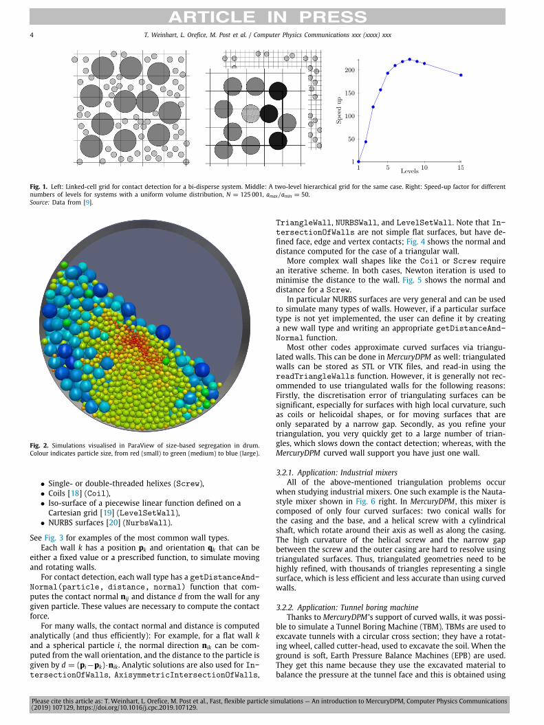
Most DPM algorithms use the linked-cell algorithm for contactdetection [15], illustrated in Fig. 1 left: Particles are placed into agrid whose cell size is the diameter of the largest particle. Thus,particles can only be in contact with particles in the same or in aneighbouring cell, reducing the number of necessary checks. For(nearly) monodispersed simulations, this algorithm is of linearcomplexity, O(N), and thus sufficiently efficient. However, theorder complexity increases to quadratic, O(N2), for highly poly-disperse simulations, because the cell size is based on the largestparticle diameter.
MercuryDPM uses the hierarchical grid (hGrid) [9,10,16], anadvanced contact detection method that uses several grids fordifferent particle sizes, as shown in Fig. 1 middle. This contactmethod gives MercuryDPM its name: hGridDPM → HgDPM →MercuryDPM . By carefully selecting the number of levels andcell sizes, linear complexity of the algorithm can be guaran-teed even for the most challenging particle size distributions.
The effectiveness of the approach has been proven theoreticallyand in simulations [9]: for highly polydisperse situations, thehierarchical grid is two orders of magnitude quicker than thelinked-cell algorithm, see Fig. 1 right. Furthermore, the CPU timevaried only minimally when comparing monodisperse, bidisperseand polydisperse systems with the same number of particles andvolume fraction [9]. This feature allows for the first time largesimulations with wide size-distributions.
The hierarchical grid algorithm is made up of two phases:mapping and contact detection. In the first phase, all particlesare mapped onto a grid level. In the second phase, the potentialcontact partners for every particle in the system are determined.Both phases are of linear complexity, and allow straightforwardparallelisation.
The two- or three-dimensional hierarchical grid is a set ofL regular grids with different cell sizes s1 < s2 < · · · < sL.Each particle p is mapped into a specific cell in the lowest levelgrid big enough to contain the particle. A new mapping is donebefore every time step, as this is cheaper than tracking changesand updating the map. It must be noted that the cell size shof each level h can be set independently, in contrast to contactdetection methods which use a tree structure for partitioningthe domain [17], where the cell sizes are taken as double thesize of the previous lower level of hierarchy, hence sh+1 = 2sh.The flexibility of independently choosing sh allows one to selectthe optimal cell sizes according to the particle size distribution,further improving the performance of the simulations [9].
The contact detection is split into two steps, and the searchis done by looping over all particles p and performing the firstand second steps consecutively for each p. The first step is acontact search at the level of insertion, using the classical linked-cell method: the search is done in the cell onto which p ismapped, and in its neighbour (surrounding) cells. Only half of thesurrounding cells are searched, to avoid testing the same particlepair twice. The second step is the cross-level search. For a givenparticle p, one searches for potential contacts only at levels ofsmaller grid size. This implies that the particle p will be checkedonly against the smaller ones, thus avoiding double checks for thesame pair of particles. See [9] for details of the algorithm.
3.1.1. Application: Segregation in rotating drumsSegregation of grains by size is a scientifically interesting
and industrially relevant problem. In industrial situations, size-distributions often range over orders of magnitude and are highlypolydispersed; whereas academic studies often consider bidisper-sity with a factor of only 2–10 in size. One key reason for thisdiscrepancy is computational cost. However, the hierarchical grid,at the heart MercuryDPM , is over three orders of magnitude fasterfor bidispersed mixtures with a size ratio of 100, and even fasterfor truly polydisperse packings; see [16] for details. Fig. 2 showsa simulation where each particle is a unique size and the ratio ofsmall to largest radii is 100. This is visualised using ParaView andwas run on a single core on a normal desktop computer in a fewhours.
3.2. Curved walls
A distinguishing feature ofMercuryDPM is its support of curvedgeometric surfaces, or walls. Many types of walls are imple-mented and ready for use, such as
• Flat walls (implemented in InfiniteWall),• Convex polygons (2D) or polyhedra (3D)
(IntersectionOfWalls),• Conical and cylindrical shapes, created by rotating a
polygon around an axis(AxisymmetricIntersectionOfWalls),
Please cite this article as: T. Weinhart, L. Orefice, M. Post et al., Fast, flexible particle simulations — An introduction to MercuryDPM, Computer Physics Communications(2019) 107129, https://doi.org/10.1016/j.cpc.2019.107129.
4 T. Weinhart, L. Orefice, M. Post et al. / Computer Physics Communications xxx (xxxx) xxx
Fig. 1. Left: Linked-cell grid for contact detection for a bi-disperse system. Middle: A two-level hierarchical grid for the same case. Right: Speed-up factor for differentnumbers of levels for systems with a uniform volume distribution, N = 125 001, amax/amin = 50.Source: Data from [9].
Fig. 2. Simulations visualised in ParaView of size-based segregation in drum.Colour indicates particle size, from red (small) to green (medium) to blue (large).
• Single- or double-threaded helixes (Screw),• Coils [18] (Coil),• Iso-surface of a piecewise linear function defined on a
Cartesian grid [19] (LevelSetWall),• NURBS surfaces [20] (NurbsWall).
See Fig. 3 for examples of the most common wall types.Each wall k has a position pk and orientation qk that can be
either a fixed value or a prescribed function, to simulate movingand rotating walls.
For contact detection, each wall type has a getDistanceAnd-Normal(particle, distance, normal) function that com-putes the contact normal nij and distance d from the wall for anygiven particle. These values are necessary to compute the contactforce.
For many walls, the contact normal and distance is computedanalytically (and thus efficiently): For example, for a flat wall kand a spherical particle i, the normal direction nik can be com-puted from the wall orientation, and the distance to the particle isgiven by d = (pi−pk)·nik. Analytic solutions are also used for In-tersectionOfWalls, AxisymmetricIntersectionOfWalls,
TriangleWall, NURBSWall, and LevelSetWall. Note that In-tersectionOfWalls are not simple flat surfaces, but have de-fined face, edge and vertex contacts; Fig. 4 shows the normal anddistance computed for the case of a triangular wall.
More complex wall shapes like the Coil or Screw requirean iterative scheme. In both cases, Newton iteration is used tominimise the distance to the wall. Fig. 5 shows the normal anddistance for a Screw.
In particular NURBS surfaces are very general and can be usedto simulate many types of walls. However, if a particular surfacetype is not yet implemented, the user can define it by creatinga new wall type and writing an appropriate getDistanceAnd-Normal function.
Most other codes approximate curved surfaces via triangu-lated walls. This can be done in MercuryDPM as well: triangulatedwalls can be stored as STL or VTK files, and read-in using thereadTriangleWalls function. However, it is generally not rec-ommended to use triangulated walls for the following reasons:Firstly, the discretisation error of triangulating surfaces can besignificant, especially for surfaces with high local curvature, suchas coils or helicoidal shapes, or for moving surfaces that areonly separated by a narrow gap. Secondly, as you refine yourtriangulation, you very quickly get to a large number of trian-gles, which slows down the contact detection; whereas, with theMercuryDPM curved wall support you have just one wall.
3.2.1. Application: Industrial mixersAll of the above-mentioned triangulation problems occur
when studying industrial mixers. One such example is the Nauta-style mixer shown in Fig. 6 right. In MercuryDPM , this mixer iscomposed of only four curved surfaces: two conical walls forthe casing and the base, and a helical screw with a cylindricalshaft, which rotate around their axis as well as along the casing.The high curvature of the helical screw and the narrow gapbetween the screw and the outer casing are hard to resolve usingtriangulated surfaces. Thus, triangulated geometries need to behighly refined, with thousands of triangles representing a singlesurface, which is less efficient and less accurate than using curvedwalls.
3.2.2. Application: Tunnel boring machineThanks to MercuryDPM ’s support of curved walls, it was possi-
ble to simulate a Tunnel Boring Machine (TBM). TBMs are used toexcavate tunnels with a circular cross section; they have a rotat-ing wheel, called cutter-head, used to excavate the soil. When theground is soft, Earth Pressure Balance Machines (EPB) are used.They get this name because they use the excavated material tobalance the pressure at the tunnel face and this is obtained using
Please cite this article as: T. Weinhart, L. Orefice, M. Post et al., Fast, flexible particle simulations — An introduction to MercuryDPM, Computer Physics Communications(2019) 107129, https://doi.org/10.1016/j.cpc.2019.107129.
T. Weinhart, L. Orefice, M. Post et al. / Computer Physics Communications xxx (xxxx) xxx 5
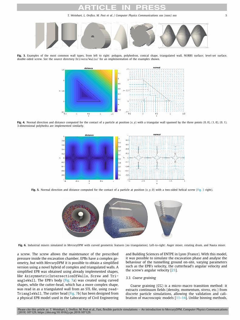
Fig. 3. Examples of the most common wall types, from left to right: polygon, polyhedron, conical shape, triangulated wall, NURBS surface; level-set surface,double-sided screw. See the source directory Drivers/Walls/ for an implementation of the examples shown.
Fig. 4. Normal direction and distance computed for the contact of a particle at position (x, y) with a triangular wall spanned by the three points (0, 0), (1, 0), (0, 1).3-dimensional polyhedra are implemented similarly.
Fig. 5. Normal direction and distance computed for the contact of a particle at position (x, y, 0) with a two-sided helical screw (Fig. 3 right).
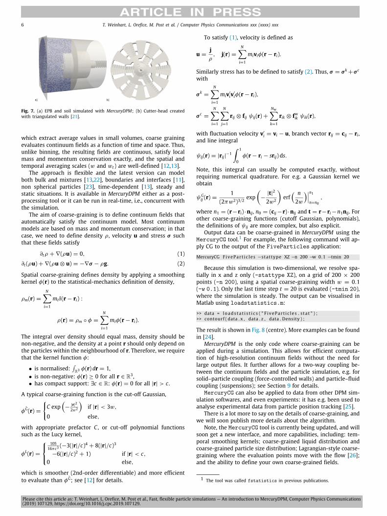
Fig. 6. Industrial mixers simulated in MercuryDPM with curved geometric features (no triangulation). Left-to-right: Auger mixer, rotating drum, and Nauta mixer.
a screw. The screw allows the maintenance of the prescribedpressure inside the excavation chamber. EPBs have a complex ge-ometry, but with MercuryDPM it is possible to obtain a simplifiedversion using a novel hybrid of complex and triangulated walls. Asimplified EPB was obtained using already implemented shapes,like AxisymmetricIntersectionOfWalls, Screw and Tri-angleWall. The EPB’s body (Fig. 7a) was created using curvedshapes, while the cutter-head, which has a more complex shape,was read in as a triangulated wall from an STL file, using read-TriangleWall. The cutter head (Fig. 7b) has been designed froma physical EPB model used in the Laboratory of Civil Engineering
and Building Sciences of ENTPE in Lyon (France). With this model,it was possible to simulate the excavation phase and analyse thebehaviour of the tunnelling ground on-site, varying parameterssuch as the EPB’s velocity, the cutterhead’s angular velocity andthe screw’s angular velocity [21].
3.3. Coarse graining
Coarse graining (CG) is a micro–macro transition method: itextracts continuum fields (density, momentum, stress, etc.) fromdiscrete particle simulations, allowing the validation and cali-bration of macroscopic models [11–14]. Unlike binning methods,
Please cite this article as: T. Weinhart, L. Orefice, M. Post et al., Fast, flexible particle simulations — An introduction to MercuryDPM, Computer Physics Communications(2019) 107129, https://doi.org/10.1016/j.cpc.2019.107129.
6 T. Weinhart, L. Orefice, M. Post et al. / Computer Physics Communications xxx (xxxx) xxx
Fig. 7. (a) EPB and soil simulated with MercuryDPM; (b) Cutter-head createdwith triangulated walls [21].
which extract average values in small volumes, coarse grainingevaluates continuum fields as a function of time and space. Thus,unlike binning, the resulting fields are continuous, satisfy localmass and momentum conservation exactly, and the spatial andtemporal averaging scales (w and wt ) are well-defined [12,13].
The approach is flexible and the latest version can modelboth bulk and mixtures [13,22], boundaries and interfaces [11],non spherical particles [23], time-dependent [13], steady andstatic situations. It is available in MercuryDPM either as a post-processing tool or it can be run in real-time, i.e., concurrent withthe simulation.
The aim of coarse-graining is to define continuum fields thatautomatically satisfy the continuum model. Most continuummodels are based on mass and momentum conservation; in thatcase, we need to define density ρ, velocity u and stress σ suchthat these fields satisfy
∂tρ +∇(ρu) = 0, (1)
∂t (ρu)+∇(ρu⊗ u) = −∇σ − ρg. (2)
Spatial coarse-graining defines density by applying a smoothingkernel φ(r) to the statistical-mechanics definition of density,
ρm(r) =N∑i=1
miδ(r− ri) :
ρ(r) = ρm ◦ φ =N∑i=1
miφ(r− ri).
The integral over density should equal mass, density should benon-negative, and the density at a point r should only depend onthe particles within the neighbourhood of r. Therefore, we requirethat the kernel function φ:
• is normalised:∫R3 φ(r) dr = 1,
• is non-negative: φ(r) ≥ 0 for all r ∈ R3,• has compact support: ∃c ∈ R: φ(r) = 0 for all |r| > c .
A typical coarse-graining function is the cut-off Gaussian,
φG̃(r) =
{C exp
(−|r|2
2w2
)if |r| < 3w,
0 else,
with appropriate prefactor C , or cut-off polynomial functionssuch as the Lucy kernel,
φL(r) =
⎧⎨⎩105
16πc3(−3(|r|/c)4 + 8(|r|/c)3
−6(|r|/c)2 + 1) if |r| < c,0 else,
which is smoother (2nd-order differentiable) and more efficientto evaluate than φG̃; see [12] for details.
To satisfy (1), velocity is defined as
u =jρ, j(r) =
N∑i=1
miviφ(r− ri).
Similarly stress has to be defined to satisfy (2). Thus, σ = σk+σc
with
σk=
N∑i=1
miv′iv′
iφ(r− ri),
σc=
N∑i=1
N∑j=1
rij ⊗ fij ψij(r)+Nw∑k=1
rik ⊗ fwik ψik(r),
with fluctuation velocity v′i = vi − u, branch vector rij = cij − ri,and line integral
ψij(r) = |rij|−1∫ 1
0φ(r− ri − srij) ds.
Note, this integral can usually be computed exactly, withoutrequiring numerical quadrature. For e.g. a Gaussian kernel weobtain
ψGij (r) =
1(2πw2)3/2
exp(−|t|2
2w2
)erf( n2w
)⏐⏐⏐n1n=n0
,
where n1 = (r−ri) ·nij, n0 = (cij−r) ·nij and t = r−ri−n1nij. Forother coarse-graining functions (cutoff Gaussian, polynomials),the definitions of ψij are more complex, but also explicit.
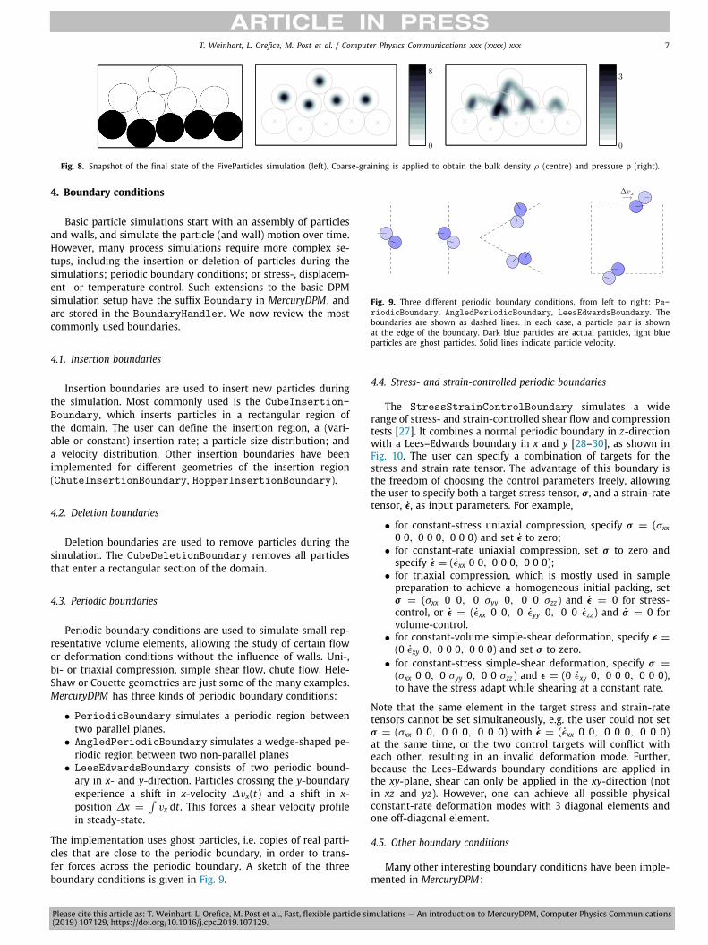
Output data can be coarse-grained in MercuryDPM using theMercuryCG tool.1 For example, the following command will ap-ply CG to the output of the FiveParticles application:
MercuryCG F ivePa r t i c l e s −stattype XZ −n 200 −w 0.1 −tmin 20
Because this simulation is two-dimensional, we resolve spa-tially in x and z only (-stattype XZ), on a grid of 200 × 200points (-n 200), using a spatial coarse-graining width w = 0.1(-w 0.1). Only the last time step t = 20 is evaluated (-tmin 20),where the simulation is steady. The output can be visualised inMatlab using loadstatistics.m:
>> data = l o ad s t a t i s t i c s ( " F i vePa r t i c l e s . s t a t " ) ;>> contourf ( data . x , data . z , data . Density ) ;
The result is shown in Fig. 8 (centre). More examples can be foundin [24].
MercuryDPM is the only code where coarse-graining can beapplied during a simulation. This allows for efficient computa-tion of high-resolution continuum fields without the need forlarge output files. It further allows for a two-way coupling be-tween the continuum fields and the particle simulation, e.g. forsolid–particle coupling (force-controlled walls) and particle–fluidcoupling (suspensions); see Section 9 for details.
MercuryCG can also be applied to data from other DPM sim-ulation softwares, and even experiments: it has e.g. been used toanalyse experimental data from particle position tracking [25].
There is a lot more to say on the details of coarse-graining, andwe will soon publish more details about the algorithm.
Note, the MercuryCG tool is currently being updated, and willsoon get a new interface, and more capabilities, including: tem-poral smoothing kernels; coarse-grained liquid distribution andcoarse-grained particle size distribution; Lagrangian-style coarse-graining where the evaluation points move with the flow [26];and the ability to define your own coarse-grained fields.
1 The tool was called fstatistics in previous publications.
Please cite this article as: T. Weinhart, L. Orefice, M. Post et al., Fast, flexible particle simulations — An introduction to MercuryDPM, Computer Physics Communications(2019) 107129, https://doi.org/10.1016/j.cpc.2019.107129.
T. Weinhart, L. Orefice, M. Post et al. / Computer Physics Communications xxx (xxxx) xxx 7
Fig. 8. Snapshot of the final state of the FiveParticles simulation (left). Coarse-graining is applied to obtain the bulk density ρ (centre) and pressure p (right).
4. Boundary conditions
Basic particle simulations start with an assembly of particlesand walls, and simulate the particle (and wall) motion over time.However, many process simulations require more complex se-tups, including the insertion or deletion of particles during thesimulations; periodic boundary conditions; or stress-, displacem-ent- or temperature-control. Such extensions to the basic DPMsimulation setup have the suffix Boundary in MercuryDPM , andare stored in the BoundaryHandler. We now review the mostcommonly used boundaries.
4.1. Insertion boundaries
Insertion boundaries are used to insert new particles duringthe simulation. Most commonly used is the CubeInsertion-Boundary, which inserts particles in a rectangular region ofthe domain. The user can define the insertion region, a (vari-able or constant) insertion rate; a particle size distribution; anda velocity distribution. Other insertion boundaries have beenimplemented for different geometries of the insertion region(ChuteInsertionBoundary, HopperInsertionBoundary).
4.2. Deletion boundaries
Deletion boundaries are used to remove particles during thesimulation. The CubeDeletionBoundary removes all particlesthat enter a rectangular section of the domain.
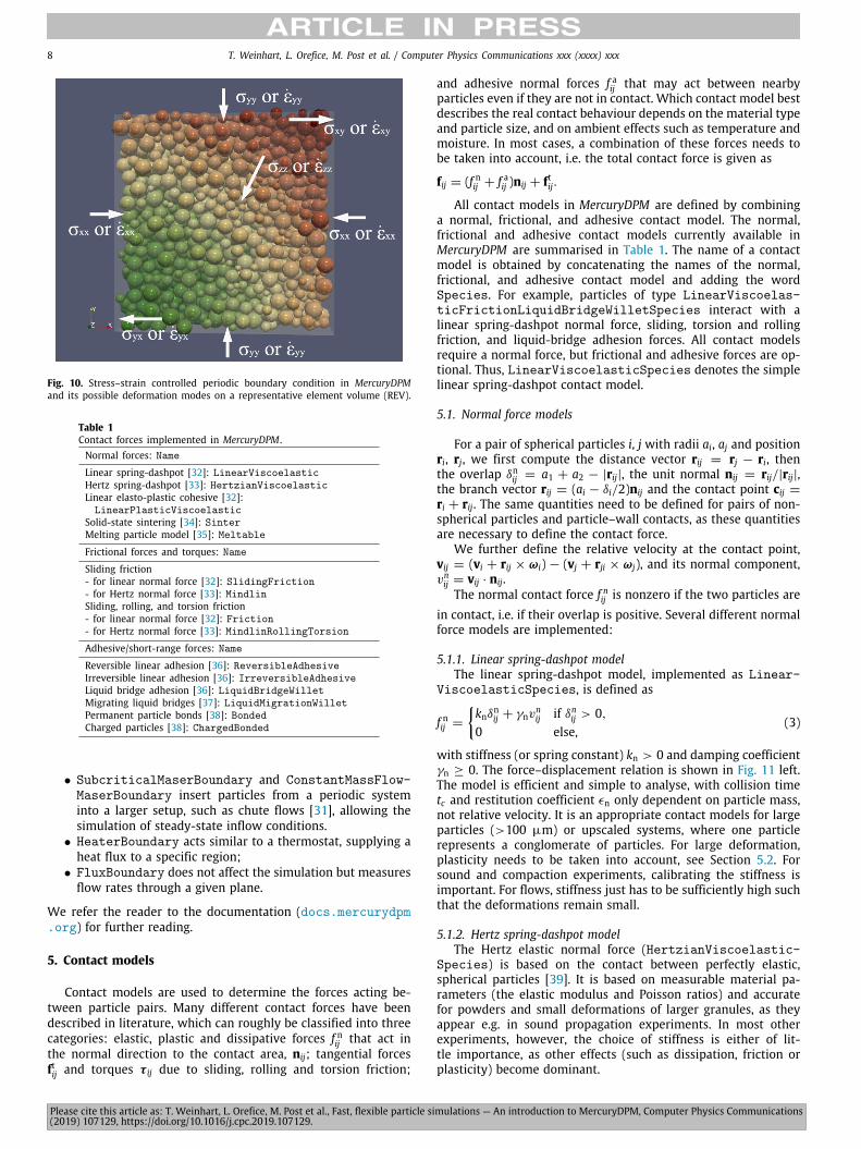
4.3. Periodic boundaries
Periodic boundary conditions are used to simulate small rep-resentative volume elements, allowing the study of certain flowor deformation conditions without the influence of walls. Uni-,bi- or triaxial compression, simple shear flow, chute flow, Hele-Shaw or Couette geometries are just some of the many examples.MercuryDPM has three kinds of periodic boundary conditions:
• PeriodicBoundary simulates a periodic region betweentwo parallel planes.• AngledPeriodicBoundary simulates a wedge-shaped pe-
riodic region between two non-parallel planes• LeesEdwardsBoundary consists of two periodic bound-
ary in x- and y-direction. Particles crossing the y-boundaryexperience a shift in x-velocity ∆vx(t) and a shift in x-position ∆x =
∫vx dt . This forces a shear velocity profile
in steady-state.
The implementation uses ghost particles, i.e. copies of real parti-cles that are close to the periodic boundary, in order to trans-fer forces across the periodic boundary. A sketch of the threeboundary conditions is given in Fig. 9.
Fig. 9. Three different periodic boundary conditions, from left to right: Pe-riodicBoundary, AngledPeriodicBoundary, LeesEdwardsBoundary. Theboundaries are shown as dashed lines. In each case, a particle pair is shownat the edge of the boundary. Dark blue particles are actual particles, light blueparticles are ghost particles. Solid lines indicate particle velocity.
4.4. Stress- and strain-controlled periodic boundaries
The StressStrainControlBoundary simulates a widerange of stress- and strain-controlled shear flow and compressiontests [27]. It combines a normal periodic boundary in z-directionwith a Lees–Edwards boundary in x and y [28–30], as shown inFig. 10. The user can specify a combination of targets for thestress and strain rate tensor. The advantage of this boundary isthe freedom of choosing the control parameters freely, allowingthe user to specify both a target stress tensor, σ, and a strain-ratetensor, ϵ̇, as input parameters. For example,
• for constant-stress uniaxial compression, specify σ = (σxx0 0, 0 0 0, 0 0 0) and set ϵ̇ to zero;• for constant-rate uniaxial compression, set σ to zero and
specify ϵ̇ = (ϵ̇xx 0 0, 0 0 0, 0 0 0);• for triaxial compression, which is mostly used in sample
preparation to achieve a homogeneous initial packing, setσ = (σxx 0 0, 0 σyy 0, 0 0 σzz) and ϵ̇ = 0 for stress-control, or ϵ̇ = (ϵ̇xx 0 0, 0 ϵ̇yy 0, 0 0 ϵ̇zz) and σ̇ = 0 forvolume-control.• for constant-volume simple-shear deformation, specify ϵ =
(0 ϵ̇xy 0, 0 0 0, 0 0 0) and set σ to zero.• for constant-stress simple-shear deformation, specify σ =
(σxx 0 0, 0 σyy 0, 0 0 σzz) and ϵ = (0 ϵ̇xy 0, 0 0 0, 0 0 0),to have the stress adapt while shearing at a constant rate.
Note that the same element in the target stress and strain-ratetensors cannot be set simultaneously, e.g. the user could not setσ = (σxx 0 0, 0 0 0, 0 0 0) with ϵ̇ = (ϵ̇xx 0 0, 0 0 0, 0 0 0)at the same time, or the two control targets will conflict witheach other, resulting in an invalid deformation mode. Further,because the Lees–Edwards boundary conditions are applied inthe xy-plane, shear can only be applied in the xy-direction (notin xz and yz). However, one can achieve all possible physicalconstant-rate deformation modes with 3 diagonal elements andone off-diagonal element.
4.5. Other boundary conditions
Many other interesting boundary conditions have been imple-mented in MercuryDPM:
Please cite this article as: T. Weinhart, L. Orefice, M. Post et al., Fast, flexible particle simulations — An introduction to MercuryDPM, Computer Physics Communications(2019) 107129, https://doi.org/10.1016/j.cpc.2019.107129.
8 T. Weinhart, L. Orefice, M. Post et al. / Computer Physics Communications xxx (xxxx) xxx
Fig. 10. Stress–strain controlled periodic boundary condition in MercuryDPMand its possible deformation modes on a representative element volume (REV).
Table 1Contact forces implemented in MercuryDPM .Normal forces: Name
Linear spring-dashpot [32]: LinearViscoelasticHertz spring-dashpot [33]: HertzianViscoelasticLinear elasto-plastic cohesive [32]:LinearPlasticViscoelastic
Solid-state sintering [34]: SinterMelting particle model [35]: Meltable
Frictional forces and torques: Name
Sliding friction- for linear normal force [32]: SlidingFriction- for Hertz normal force [33]: MindlinSliding, rolling, and torsion friction- for linear normal force [32]: Friction- for Hertz normal force [33]: MindlinRollingTorsion
Adhesive/short-range forces: Name
Reversible linear adhesion [36]: ReversibleAdhesiveIrreversible linear adhesion [36]: IrreversibleAdhesiveLiquid bridge adhesion [36]: LiquidBridgeWilletMigrating liquid bridges [37]: LiquidMigrationWilletPermanent particle bonds [38]: BondedCharged particles [38]: ChargedBonded
• SubcriticalMaserBoundary and ConstantMassFlow-MaserBoundary insert particles from a periodic systeminto a larger setup, such as chute flows [31], allowing thesimulation of steady-state inflow conditions.• HeaterBoundary acts similar to a thermostat, supplying a
heat flux to a specific region;• FluxBoundary does not affect the simulation but measures
flow rates through a given plane.
We refer the reader to the documentation (docs.mercurydpm.org) for further reading.
5. Contact models
Contact models are used to determine the forces acting be-tween particle pairs. Many different contact forces have beendescribed in literature, which can roughly be classified into threecategories: elastic, plastic and dissipative forces f nij that act inthe normal direction to the contact area, nij; tangential forcesftij and torques τ ij due to sliding, rolling and torsion friction;
and adhesive normal forces f aij that may act between nearbyparticles even if they are not in contact. Which contact model bestdescribes the real contact behaviour depends on the material typeand particle size, and on ambient effects such as temperature andmoisture. In most cases, a combination of these forces needs tobe taken into account, i.e. the total contact force is given as
fij = (f nij + f aij )nij + ftij.
All contact models in MercuryDPM are defined by combininga normal, frictional, and adhesive contact model. The normal,frictional and adhesive contact models currently available inMercuryDPM are summarised in Table 1. The name of a contactmodel is obtained by concatenating the names of the normal,frictional, and adhesive contact model and adding the wordSpecies. For example, particles of type LinearViscoelas-ticFrictionLiquidBridgeWilletSpecies interact with alinear spring-dashpot normal force, sliding, torsion and rollingfriction, and liquid-bridge adhesion forces. All contact modelsrequire a normal force, but frictional and adhesive forces are op-tional. Thus, LinearViscoelasticSpecies denotes the simplelinear spring-dashpot contact model.
5.1. Normal force models
For a pair of spherical particles i, j with radii ai, aj and positionri, rj, we first compute the distance vector rij = rj − ri, thenthe overlap δnij = a1 + a2 − |rij|, the unit normal nij = rij/|rij|,the branch vector rij = (ai − δi/2)nij and the contact point cij =ri + rij. The same quantities need to be defined for pairs of non-spherical particles and particle–wall contacts, as these quantitiesare necessary to define the contact force.
We further define the relative velocity at the contact point,vij = (vi + rij × ωi) − (vj + rji × ωj), and its normal component,vnij = vij · nij.
The normal contact force f nij is nonzero if the two particles arein contact, i.e. if their overlap is positive. Several different normalforce models are implemented:
5.1.1. Linear spring-dashpot modelThe linear spring-dashpot model, implemented as Linear-
ViscoelasticSpecies, is defined as
f nij ={knδnij + γnv
nij if δnij > 0,
0 else,(3)
with stiffness (or spring constant) kn > 0 and damping coefficientγn ≥ 0. The force–displacement relation is shown in Fig. 11 left.The model is efficient and simple to analyse, with collision timetc and restitution coefficient ϵn only dependent on particle mass,not relative velocity. It is an appropriate contact models for largeparticles (>100 µm) or upscaled systems, where one particlerepresents a conglomerate of particles. For large deformation,plasticity needs to be taken into account, see Section 5.2. Forsound and compaction experiments, calibrating the stiffness isimportant. For flows, stiffness just has to be sufficiently high suchthat the deformations remain small.
5.1.2. Hertz spring-dashpot modelThe Hertz elastic normal force (HertzianViscoelastic-
Species) is based on the contact between perfectly elastic,spherical particles [39]. It is based on measurable material pa-rameters (the elastic modulus and Poisson ratios) and accuratefor powders and small deformations of larger granules, as theyappear e.g. in sound propagation experiments. In most otherexperiments, however, the choice of stiffness is either of lit-tle importance, as other effects (such as dissipation, friction orplasticity) become dominant.
Please cite this article as: T. Weinhart, L. Orefice, M. Post et al., Fast, flexible particle simulations — An introduction to MercuryDPM, Computer Physics Communications(2019) 107129, https://doi.org/10.1016/j.cpc.2019.107129.
T. Weinhart, L. Orefice, M. Post et al. / Computer Physics Communications xxx (xxxx) xxx 9
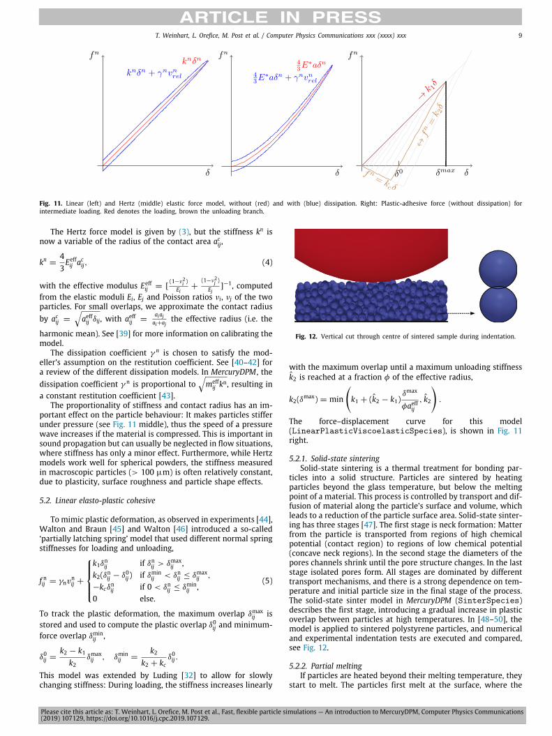
Fig. 11. Linear (left) and Hertz (middle) elastic force model, without (red) and with (blue) dissipation. Right: Plastic-adhesive force (without dissipation) forintermediate loading. Red denotes the loading, brown the unloading branch.
The Hertz force model is given by (3), but the stiffness kn isnow a variable of the radius of the contact area acij,
kn =43Eeffij acij, (4)
with the effective modulus Eeffij = [
(1−ν2i )Ei+
(1−ν2j )
Ej]−1, computed
from the elastic moduli Ei, Ej and Poisson ratios νi, νj of the twoparticles. For small overlaps, we approximate the contact radiusby acij =
√aeffij δij, with aeffij =
aiajai+aj
the effective radius (i.e. the
harmonic mean). See [39] for more information on calibrating themodel.
The dissipation coefficient γ n is chosen to satisfy the mod-eller’s assumption on the restitution coefficient. See [40–42] fora review of the different dissipation models. In MercuryDPM , thedissipation coefficient γ n is proportional to
√meff
ij kn, resulting ina constant restitution coefficient [43].
The proportionality of stiffness and contact radius has an im-portant effect on the particle behaviour: It makes particles stifferunder pressure (see Fig. 11 middle), thus the speed of a pressurewave increases if the material is compressed. This is important insound propagation but can usually be neglected in flow situations,where stiffness has only a minor effect. Furthermore, while Hertzmodels work well for spherical powders, the stiffness measuredin macroscopic particles (> 100 µm) is often relatively constant,due to plasticity, surface roughness and particle shape effects.
5.2. Linear elasto-plastic cohesive
To mimic plastic deformation, as observed in experiments [44],Walton and Braun [45] and Walton [46] introduced a so-called‘partially latching spring’ model that used different normal springstiffnesses for loading and unloading,
f nij = γnvnij +
⎧⎪⎪⎨⎪⎪⎩k1δnij if δnij > δmax
ij ,k2(δnij − δ
0ij) if δmin
ij < δnij ≤ δmaxij ,
−kcδnij if 0 < δnij ≤ δminij ,
0 else.
(5)
To track the plastic deformation, the maximum overlap δmaxij is
stored and used to compute the plastic overlap δ0ij and minimum-force overlap δmin
ij ,
δ0ij =k2 − k1
k2δmaxij , δmin
ij =k2
k2 + kcδ0ij .
This model was extended by Luding [32] to allow for slowlychanging stiffness: During loading, the stiffness increases linearly
Fig. 12. Vertical cut through centre of sintered sample during indentation.
with the maximum overlap until a maximum unloading stiffnessk̂2 is reached at a fraction φ of the effective radius,
k2(δmax) = min
(k1 + (k̂2 − k1)
δmax
φaeffij, k̂2
).
The force–displacement curve for this model(LinearPlasticViscoelasticSpecies), is shown in Fig. 11right.
5.2.1. Solid-state sinteringSolid-state sintering is a thermal treatment for bonding par-
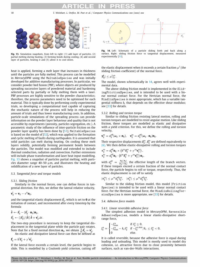
ticles into a solid structure. Particles are sintered by heatingparticles beyond the glass temperature, but below the meltingpoint of a material. This process is controlled by transport and dif-fusion of material along the particle’s surface and volume, whichleads to a reduction of the particle surface area. Solid-state sinter-ing has three stages [47]. The first stage is neck formation: Matterfrom the particle is transported from regions of high chemicalpotential (contact region) to regions of low chemical potential(concave neck regions). In the second stage the diameters of thepores channels shrink until the pore structure changes. In the laststage isolated pores form. All stages are dominated by differenttransport mechanisms, and there is a strong dependence on tem-perature and initial particle size in the final stage of the process.The solid-state sinter model in MercuryDPM (SinterSpecies)describes the first stage, introducing a gradual increase in plasticoverlap between particles at high temperatures. In [48–50], themodel is applied to sintered polystyrene particles, and numericaland experimental indentation tests are executed and compared,see Fig. 12.
5.2.2. Partial meltingIf particles are heated beyond their melting temperature, they
start to melt. The particles first melt at the surface, where the
Please cite this article as: T. Weinhart, L. Orefice, M. Post et al., Fast, flexible particle simulations — An introduction to MercuryDPM, Computer Physics Communications(2019) 107129, https://doi.org/10.1016/j.cpc.2019.107129.
10 T. Weinhart, L. Orefice, M. Post et al. / Computer Physics Communications xxx (xxxx) xxx
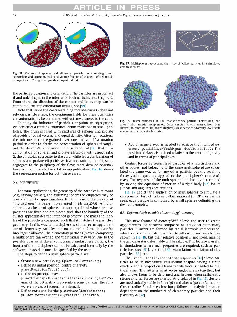
Fig. 13. Simulation snapshots, from left to right: (1) add layer of particles, (2)partial melting during heating, (3) forming bonds during cooling, (4) add secondlayer of particles, heating it and (5) allow it to cool down.
heat is applied, forming a melt layer that increases in thicknessuntil the particles are fully melted. This process can be modelledin MercuryDPM using the MeltableSpecies and was initiallydeveloped for additive manufacturing processes. In particular, weconsider powder bed fusion (PBF), where objects are produced byspreading successive layers of powdered material and hardeningselected parts by partially or fully melting them with a laser.PBF processes are highly sensitive to the powder characteristics;therefore, the process parameters need to be optimised for eachmaterial. This is typically done by performing costly experimentaltrials, so developing a computational tool capable of capturingthe stochastic nature of the process will help in reducing theamount of trials and thus lower manufacturing costs. In addition,particle-scale simulations of the spreading process can provideinformation on the powder layer behaviour and quality that is notaccessible by experiments (porosity, particles segregation, etc.). Aparametric study of the influence of inter-particle friction on thepowder layer quality has been done by [51]. MeltableSpeciesis based on the model of [52], which was applied to the formationand cyclic melting of faults during earthquakes. It is assumed thatsolid particles can melt during heating. On cooling these meltlayers solidify, potentially forming permanent bonds betweenthe particles. The model was modified and extended to includethermal conduction, radiation and convection. Further extensionswill include phase transformation and laser heat input modelling.Fig. 13 shows a snapshot of particles partial melting, with parti-cles diameter range 40–50 µm, and illustrates the heating andsolidification of a new layer of particles.
5.3. Tangential force and torque models
5.3.1. Sliding frictionSimilarly to the normal forces, one can define forces in tan-
gential direction. For this, we define the lateral relative velocity,
vlij = vij − vnnij,
and the tangential elastic displacement δlij, which is set to 0 at theinitiation of contact, and incremented after every timestep by theformula
δ̃← δlij − (δlij · nij)nij,
δlij ← (|δlij|/|δ̃|) δ̃+ vlij∆t. (6)
The two-step procedure is necessary to keep the tangential dis-placement in the tangential plane while the particle pair rotates.Note that for a fixed normal direction nij, we obtain d
dt δlij = vlij.
An elastic and dissipative lateral force can then be defined as
flij = klδνij + γlvlij.
If the lateral force exceeds a certain level, the particle begins toslide. This is modelled by a Coulomb yield criterion, cutting off
Fig. 14. Left: Schematic of a particle sliding forth and back along asurface, Right: sliding friction force vs tangential displacement, measuredexperimentally [53].
the elastic displacement when it exceeds a certain fraction µl (thesliding friction coefficient) of the normal force.
|flij| ≤ µlf nij .
The model, shown schematically in 14, agrees well with experi-mental data.
The above sliding friction model is implemented in the Slid-ingFrictionSpecies, and is intended to be used with a lin-ear normal contact force. For the Hertzian normal force, theMindlinSpecies is more appropriate, which has a variable tan-gential stiffness kt that depends on the effective shear modulus;see [33] for details.
5.3.2. Rolling and torsion torqueSimilar to sliding friction resisting lateral motion, rolling and
torsion torques are modelled to resist angular motion. Like slidingfriction, these torques are modelled as elastic and dissipativewith a yield criterion. For this, we define the rolling and torsionvelocity,
vroij = aeffij (ωij × nij), vtoij = aeffij (ωij · nij)nij.
Their respective displacements δroij , δtoij are defined equivalently to
(6). We then define elastic-dissipative rolling and torsion torques
τroij = aeffij nij ×
(kroδroij + γ
rovroij),
τtoij = aeffij nij ·
(ktoδtoij + γ
tovtoij)nij,
with aeffij =|rij| |rji||rij|+|rji|
the effective length of the branch vectors.If these torques exceed a certain fraction of the normal contactforce, the particle begins to roll or torque, respectively. Thus, theelastic displacement is cut off to satisfy
|τroij | ≤ µ
roaeffij fnij , |τ
toij | ≤ µ
toaeffij fnij .
Similar to the sliding friction model, this model (FrictionSpecies) is intended to be used with a linear normal contactforce. For the Hertzian normal force, the MindlinRollingTor-sionSpecies is more appropriate, see [33] for details.
5.4. Adhesive force models
5.4.1. Linear reversible adhesive forceThe simplest adhesion model in MercuryDPM , Reversible
AdhesiveSpecies, models a linear elastic-dissipative short-range force,
f aij =
⎧⎨⎩−f amax if δnij ≥ 0,−f amax − kcδnij if −f a,max
ij /kc ≤ δnij < 0,0 else.
It is called reversible, because the adhesive force is equal duringloading and unloading. This model is mostly used to model drycohesion, i.e. attractive forces due to close proximity betweensurfaces, such as van-der-Walls interactions.
Please cite this article as: T. Weinhart, L. Orefice, M. Post et al., Fast, flexible particle simulations — An introduction to MercuryDPM, Computer Physics Communications(2019) 107129, https://doi.org/10.1016/j.cpc.2019.107129.
T. Weinhart, L. Orefice, M. Post et al. / Computer Physics Communications xxx (xxxx) xxx 11
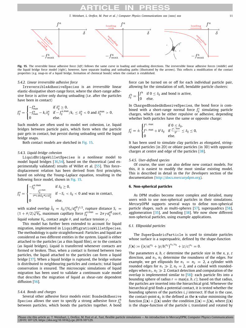
Fig. 15. The reversible linear adhesive force (left) follows the same curve in loading and unloading directions. The irreversible linear adhesive forces (middle) andthe liquid bridge force model (right), however, have separate loading and unloading paths (illustrated by the arrows). This reflects a modification of the contactproperties (e.g. snap-in of a liquid bridge, formation of chemical bonds) when the contact is established.
5.4.2. Linear irreversible adhesive forceIrreversibleAdhesiveSpecies is an irreversible linear
elastic-dissipative short-range force, where the short-range adhe-sive force is active only during unloading (i.e. after the particleshave been in contact)
f aij =
⎧⎨⎩−f amax if δnij ≥ 0,−f amax − kcδnij if− f a,max
ij /kc ≤ δnij < 0 and δmaxij > 0,
0 else.
Such models are often used to model wet cohesion, i.e. liquidbridges between particle pairs, which form when the particlepair gets in contact, but persist during unloading until the liquidbridge snaps.
Both contact models are sketched in Fig. 15.
5.4.3. Liquid-bridge cohesionLiquidBridgeWilletSpecies is a nonlinear model to
model liquid bridges [36,54], based on the theoretical (and ex-perimentally validated) results of Willet et al. [55]. This force–displacement relation has been derived from first principles,based on solving the Young–Laplace equation, resulting in thefollowing force model, shown in Fig. 15.
f aij =
⎧⎪⎪⎨⎪⎪⎩−f a,max
ij if δij ≥ 0,
−f a,maxij
1+1.05δ̂ij+2.5δ̂2ijif −Sc < δij < 0 and was in contact,
0 else,
with scaled overlap δ̂ij = δij/(Vb/aeffij )1/2, rupture distance Sc =
(1 + θ/2) 3√Vb, maximum capillary force f a,maxij = 2πγ aeffij cos θ ,
liquid volume Vb, contact angle θ , and surface tension γ .This model has further been extended to account for liquid
migration, implemented in LiquidMigrationWilletSpecies.The methodology is quite straightforward: Particles and liquid areconsidered as two different entities in the system. Liquid is eitherattached to the particles (as a thin liquid film), or to the contacts(as liquid bridges). Liquid is transferred whenever contacts areformed or broken. Thus, when a contact is formed between twoparticles, the liquid attached to the particles can form a liquidbridge [37]. When a liquid bridge is ruptured, the bridge volumeis distributed to neighbouring particles and contacts; total liquidconservation is ensured. The microscopic simulations of liquidmigration has been used to validate a continuum scale modelthat describes the migration of liquid as shear-rate dependentdiffusion [56].
5.4.4. Bonds and chargesSeveral other adhesive force models exist: BondedAdhesive
Species allows the user to specify a strong adhesive force f bijbetween particles, which bonds the particles together. A bond
force can be turned on or off for each individual particle pair,allowing for the simulation of soft, bendable particle clusters:
f bij ={f b if 0 ≤ δij and bond is active,0 else.
In ChargedBondedAdhesiveSpecies, the bond force is com-bined with a short-range normal force f cij simulating particlecharges, which can be either repulsive or adhesive, dependingwhether both particles have the same or opposite charge:
f cij = ±
⎧⎨⎩f c, max if 0 ≤ δij,f c, max
+ kcδij if f c, max
kc ≤ δij ≤ 0,0 else.
It has been used to simulate clay particles as elongated, string-shaped particles (in 2D) or oblate particles (in 3D) with oppositecharges at centre and edge of the particles [38].
5.4.5. User-defined speciesOf course, the user can also define new contact models. For
this, it is easiest to modify the most similar existing model.This is described in detail in the For Developers section of thedocumentation (http://docs.mercurydpm.org).
6. Non-spherical particles
As DPM studies become more complex and detailed, manyusers wish to use non-spherical particles in their simulations.MercuryDPM supports several ways to define non-sphericalparticle shapes, such as multi-spheres [57], superquadrics [58],agglomeration [35], and bonding [38]. We now show differentnon-spherical particles, using example applications.
6.1. Ellipsoidal particles
The SuperQuadricParticle is used to simulate particleswhose surface is a superquadric, defined by the shape-function
f (x) :=(|x/a|n2 + |y/b|n2
)n1/n2+ |z/c|n1 = 0.
The parameters a, b, c determine the particle size in the x, y, zdirection, and n1, n2 determine the roundness of the edges. Forexample, we get ellipsoids for n1 = n2 = 2, a cylinder withrounded edges for n1 ≫ 2, n2 = 2, and a cuboid with rounded-edges when n1, n2 ≫ 2. Contact detection and computation of theoverlap is implemented similar to [58]: each particle fits into abounding sphere of radius r = max(a, b, c); based on that radius,the particles are inserted into the hierarchical grid. Whenever thehierarchical grid finds a potential contact, it is tested whether thebounding spheres of the particles i, j intersect. If that is the case,the contact-point cij is the defined as the x-value minimising thefunction fi(x)+ fj(x) under the condition fi(x) = fj(x), where fi(x)is the shape-function of the particle i, translated and rotated by
Please cite this article as: T. Weinhart, L. Orefice, M. Post et al., Fast, flexible particle simulations — An introduction to MercuryDPM, Computer Physics Communications(2019) 107129, https://doi.org/10.1016/j.cpc.2019.107129.
12 T. Weinhart, L. Orefice, M. Post et al. / Computer Physics Communications xxx (xxxx) xxx
Fig. 16. Mixtures of spheres and ellipsoidal particles in a rotating drum,screenshots and coarse-grained solid volume fraction of spheres. (left) ellipsoidsof aspect ratio 2, (right) ellipsoids of aspect ratio 4.
the particle’s position and orientation. The particles are in contactif and only if cij is in the interior of both particles, i.e., fi(cij) < 0.From there, the direction of the contact and its overlap can becomputed. For implementation details, see [59].
Note that, since the coarse-graining tool MercuryCG does notrely on particle shape, the continuum fields for these quantitiescan automatically be computed without any changes to the code.
To study the influence of particle elongation on segregation,we construct a rotating cylindrical drum made out of small par-ticles. The drum is filled with mixtures of spheres and prolateellipsoids of equal volume and equal density. After ten rotations,the mixture is coarse-grained over one and a half a rotationperiod in order to obtain the concentration of spheres through-out the drum. We confirmed the observation of [60] that for acombination of spheres and prolate ellipsoids with aspect ratio2, the ellipsoids segregate to the core, while for a combination ofspheres and prolate ellipsoids with aspect ratio 4, the ellipsoidssegregate to the periphery of the flow; more detailed observa-tions will be presented in a follow-up publication. Fig. 16 showsthe segregation profile for both these cases.
6.2. Multispheres
For some applications, the geometry of the particles is relevant(e.g., railway ballast), and assuming spheres or ellipsoids may bea very simplistic approximation. For this reason, the concept of‘‘multispheres’’ is being implemented in MercuryDPM . A multi-sphere is a cluster of spheres (or superquadrics) whose relativepositions are fixed and are placed such that the boundary of thecluster approximates the intended geometry. The mass and iner-tia of the particle is computed such that it matches the particle’sgeometry. In this way, a multisphere is similar to an agglomer-ate of elementary particles, but no internal deformation and/orbreakage is allowed. The elementary particles (slaves) composinga multisphere can overlap and their radius may vary. Due to thepossible overlap of slaves composing a multisphere particle, theinertia of the multisphere cannot be calculated internally by thesoftware; instead, it must be specified by the user.
The steps to define a multisphere particle are:
• Create a new particle, e.g. SphericalParticle p;• Define its initial position (centre of gravity):p.setPosition(Vec3D pos);• Define its principal axes:p.setPrincipalDirections(Matrix3D dir); Each col-umn of the 3D matrix represents a principal axis; the soft-ware enforces orthogonality internally• Define mass and inertia: p.setMass(double mass);p0.setInertia(MatrixSymmetric3D inertia);
Fig. 17. Multispheres reproducing the shape of ballast particles in a simulatedcompression test.
Fig. 18. Cluster composed of 1000 monodispersed particles before (left) andafter (right) uniaxial compression. Color denotes kinetic energy, from blue(lowest) to green (medium) to red (highest). Most particles have very low kineticenergy, indicating a stable cluster.
• Add as many slaves as needed to achieve the intended ge-ometry: p.addSlave(Vec3D pos, double radius); Theposition of slaves is defined relative to the centre of gravityand in terms of principal axes.
Contact forces between slave particles of a multisphere andother bodies (not belonging to the same multisphere) are calcu-lated the same way as for any other particle, but the resultingforces and torques are applied to the multisphere’s centre-of-mass. The response of the multisphere is ultimately determinedby solving the equations of motion of a rigid body [57] for its(linear and angular) accelerations.
Fig. 17 depicts the application of multispheres to simulate acompression test of railway ballast material (in 2D). As can beseen, each particle is composed by small spheres delimiting thedesired geometry.
6.3. Deformable/breakable clusters (agglomerates)
This new feature of MercuryDPM allows the user to createagglomerates (or clusters) composed of individual elementaryparticles. Clusters are formed by radial isotropic compression,which causes the cluster particles to adhere to one another, asshown in Fig. 18, but their relative position is not fixed, makingthe agglomerates deformable and breakable. This feature is usefulin simulations where such properties are required, such as par-ticle breakage [61], tableting [62], granulation, simulation of clayparticles [63], etc.
The LinearPlasticViscoelasticSpecies [32] allows par-ticles to be in mechanical equilibrium despite having a finiteoverlap, and a proportional finite tensile force is needed to pullthem apart. The latter is what keeps agglomerates together, butalso allows them to be deformed and broken when sufficientlystrong external forces are exerted. As displayed in Fig. 18, clustersare mechanically stable before (left) and after (right) deformation.Cluster radius R and mass fraction ζ follow an analytical relationdependent on the number N of elementary particles and theirplasticity φ [32].
Please cite this article as: T. Weinhart, L. Orefice, M. Post et al., Fast, flexible particle simulations — An introduction to MercuryDPM, Computer Physics Communications(2019) 107129, https://doi.org/10.1016/j.cpc.2019.107129.
T. Weinhart, L. Orefice, M. Post et al. / Computer Physics Communications xxx (xxxx) xxx 13
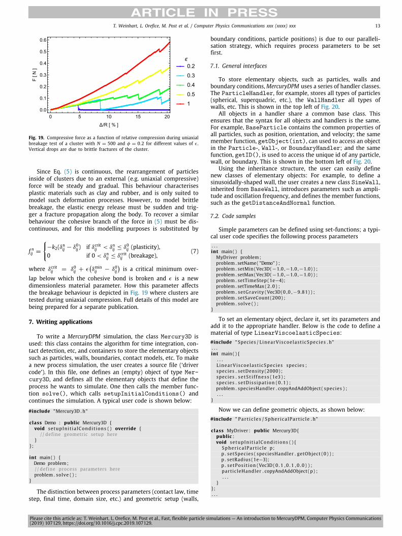
Fig. 19. Compressive force as a function of relative compression during uniaxialbreakage test of a cluster with N = 500 and φ = 0.2 for different values of ϵ.Vertical drops are due to brittle fractures of the cluster.
Since Eq. (5) is continuous, the rearrangement of particlesinside of clusters due to an external (e.g. uniaxial compressive)force will be steady and gradual. This behaviour characterisesplastic materials such as clay and rubber, and is only suited tomodel such deformation processes. However, to model brittlebreakage, the elastic energy release must be sudden and trig-ger a fracture propagation along the body. To recover a similarbehaviour the cohesive branch of the force in (5) must be dis-continuous, and for this modelling purposes is substituted by
f nij =
{−k2(δnij − δ
0ij) if δcritij < δnij ≤ δ
0ij (plasticity),
0 if 0 < δnij ≤ δcritij (breakage),
(7)
where δcritij = δ0ij + ϵ(δminij − δ0ij
)is a critical minimum over-
lap below which the cohesive bond is broken and ϵ is a newdimensionless material parameter. How this parameter affectsthe breakage behaviour is depicted in Fig. 19 where clusters aretested during uniaxial compression. Full details of this model arebeing prepared for a separate publication.
7. Writing applications
To write a MercuryDPM simulation, the class Mercury3D isused: this class contains the algorithm for time integration, con-tact detection, etc, and containers to store the elementary objectssuch as particles, walls, boundaries, contact models, etc. To makea new process simulation, the user creates a source file (‘drivercode’). In this file, one defines an (empty) object of type Mer-cury3D, and defines all the elementary objects that define theprocess he wants to simulate. One then calls the member func-tion solve(), which calls setupInitialConditions() andcontinues the simulation. A typical user code is shown below:
#include "Mercury3D . h"
class Demo : public Mercury3D {void se tup In i t i a lCondi t ions ( ) override {
/ / define geometric setup here}
} ;
int main ( ) {Demo problem ;/ / define process parameters hereproblem . solve ( ) ;
}
The distinction between process parameters (contact law, timestep, final time, domain size, etc.) and geometric setup (walls,
boundary conditions, particle positions) is due to our paralleli-sation strategy, which requires process parameters to be setfirst.
7.1. General interfaces
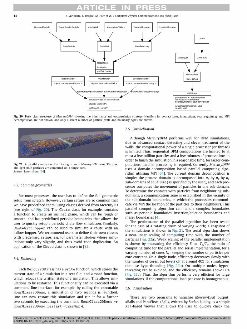
To store elementary objects, such as particles, walls andboundary conditions,MercuryDPM uses a series of handler classes.The ParticleHandler, for example, stores all types of particles(spherical, superquadric, etc.), the WallHandler all types ofwalls, etc. This is shown in the top left of Fig. 20.
All objects in a handler share a common base class. Thisensures that the syntax for all objects and handlers is the same.For example, BaseParticle contains the common properties ofall particles, such as position, orientation, and velocity; the samemember function, getObject(int), can used to access an objectin the Particle-, Wall-, or BoundaryHandler; and the samefunction, getID(), is used to access the unique id of any particle,wall, or boundary. This is shown in the bottom left of Fig. 20.
Using the inheritance structure, the user can easily definenew classes of elementary objects: For example, to define asinusoidally-shaped wall, the user creates a new class SineWall,inherited from BaseWall, introduces parameters such as ampli-tude and oscillation frequency, and defines the member functions,such as the getDistanceAndNormal function.
7.2. Code samples
Simple parameters can be defined using set-functions; a typi-cal user code specifies the following process parameters. . .int main ( ) {
MyDriver problem ;problem . setName( "Demo" ) ;problem . setMin (Vec3D(−1.0 ,−1.0 ,−1.0) ) ;problem . setMax (Vec3D(−1.0 ,−1.0 ,−1.0) ) ;problem . setTimeStep (1e−4);problem . setTimeMax (2 . 0 ) ;problem . setGravity (Vec3D(0 ,0 ,−9.81) ) ;problem . setSaveCount (200) ;problem . solve ( ) ;
}
To set an elementary object, declare it, set its parameters andadd it to the appropriate handler. Below is the code to define amaterial of type LinearViscoelasticSpecies:#include " Species / L inearViscoe las t i cSpec ies . h". . .int main ( ) {
. . .L inearViscoe las t i cSpec ies species ;species . setDensity (2000) ;species . s e t S t i f f n e s s (1e3 ) ;species . se tDiss ipat ion (0 . 1 ) ;problem . speciesHandler . copyAndAddObject ( species ) ;. . .
}
Now we can define geometric objects, as shown below:#include " Pa r t i c l e s / Spher i ca lPa r t i c l e . h"
class MyDriver : public Mercury3D{public :void se tup In i t i a lCondi t ions ( ) {
Spher i ca lPa r t i c l e p;p . setSpecies ( speciesHandler . getObject (0) ) ;p . setRadius (1e−3);p . se tPos i t ion (Vec3D (0 . 1 , 0 . 1 , 0 . 0 ) ) ;part ic leHandler . copyAndAddObject (p) ;. . .
}} ;. . .
Please cite this article as: T. Weinhart, L. Orefice, M. Post et al., Fast, flexible particle simulations — An introduction to MercuryDPM, Computer Physics Communications(2019) 107129, https://doi.org/10.1016/j.cpc.2019.107129.
14 T. Weinhart, L. Orefice, M. Post et al. / Computer Physics Communications xxx (xxxx) xxx
Fig. 20. Basic class structure of MercuryDPM , showing the inheritance and encapsulation strategy. Handlers for contact laws, interactions, coarse-graining, and MPIdecomposition are not shown, and only a select number of particle, wall, and boundary types are shown.
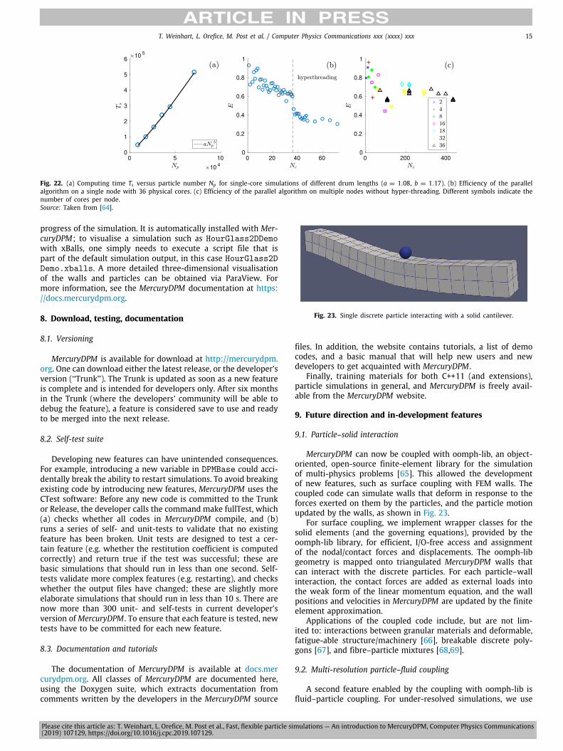
Fig. 21. A parallel simulation of a rotating drum in MercuryDPM using 36 cores.The light blue particles are computed on a single core.Source: Taken from [64].
7.3. Common geometries
For most processes, the user has to define the full geometricsetup from scratch. However, certain setups are so common thatwe have predefined them, using classes derived from Mercury3D(see right of Fig. 20). The Chute class, for example, containsa function to create an inclined plane, which can be rough orsmooth, and has predefined periodic boundaries that allows theuser to quickly setup a periodic chute flow simulation. Similarly,ChuteWithHopper can be used to simulate a chute with aninflow hopper. We recommend users to define their own classeswith predefined setups, e.g. for parameter studies where simu-lations only vary slightly, and thus avoid code duplication. Anapplication of the Chute class is shown in [35].
7.4. Restarting
Each Mercury3D class has a write function, which stores thecurrent state of a simulation in a text file; and a read function,which reloads the written state of a simulation. This allows sim-ulations to be restarted. This functionality can be executed via acommand-line interface: for example, by calling the executableHourGlass2DDemo, a simulation of two seconds is launched.One can now restart this simulation and run it for a furthertwo seconds by executing the command HourGlass2DDemo -rHourGlass2DDemo.restart -timeMax 4.
7.5. Parallelisation
Although MercuryDPM performs well for DPM simulations,due to advanced contact detecting and clever treatment of thewalls, the computational power of a single processor (or thread)is limited. Thus, sequential DPM computations are limited to atmost a few million particles and a few minutes of process time. Inorder to finish the simulation in a reasonable time, for larger com-putations, parallel processing is required. Currently MercuryDPMuses a domain-decomposition based parallel computing algo-rithm utilising MPI [64]. The current domain decomposition issimple: the process domain is decomposed into nx-by-ny-by-nzsub-domains of equal size (as specified by the user), and each pro-cessor computes the movement of particles in one sub-domain.To determine the contacts with particles from neighbouring sub-domains, a communication zone is established in the vicinity ofthe sub-domain boundaries, in which the processors communi-cate via MPI the location of the particles to their neighbours. Thisparallel computing algorithm can handle complex boundariessuch as periodic boundaries, insertion/deletion boundaries andmaser boundaries [4].
The performance of the parallel algorithm has been testedfor the case of a rotating drum of varying width; a snapshot ofthe simulations is shown in Fig. 21. The serial algorithm showsa near-linear scaling of computing time with the number ofparticles (Fig. 22a). Weak scaling of the parallel implementationis shown by measuring the efficiency E = Tp/Ts, the ratio ofcomputing time for the parallel and serial implementation, for avarying number of cores Nc , keeping the number of particles percore constant. On a single node, efficiency decreases slowly withthe number of cores, but levels off at around 40% for simulationsthat use hyperthreading (Fig. 22b). On multiple nodes, hyper-threading can be avoided, and the efficiency remains above 60%(Fig. 22c). Thus, the algorithm performs very efficient for largesimulations, if the computational load per core is homogeneous.
7.6. Visualisation
There are two programs to visualise MercuryDPM output:xBalls and ParaView. xBalls, written by Stefan Luding, is a simpleX11-based viewer that allows the user to quickly check the
Please cite this article as: T. Weinhart, L. Orefice, M. Post et al., Fast, flexible particle simulations — An introduction to MercuryDPM, Computer Physics Communications(2019) 107129, https://doi.org/10.1016/j.cpc.2019.107129.
T. Weinhart, L. Orefice, M. Post et al. / Computer Physics Communications xxx (xxxx) xxx 15
Fig. 22. (a) Computing time Ts versus particle number Np for single-core simulations of different drum lengths (a = 1.08, b = 1.17). (b) Efficiency of the parallelalgorithm on a single node with 36 physical cores. (c) Efficiency of the parallel algorithm on multiple nodes without hyper-threading. Different symbols indicate thenumber of cores per node.Source: Taken from [64].
progress of the simulation. It is automatically installed with Mer-curyDPM; to visualise a simulation such as HourGlass2DDemowith xBalls, one simply needs to execute a script file that ispart of the default simulation output, in this case HourGlass2DDemo.xballs. A more detailed three-dimensional visualisationof the walls and particles can be obtained via ParaView. Formore information, see the MercuryDPM documentation at https://docs.mercurydpm.org.
8. Download, testing, documentation
8.1. Versioning
MercuryDPM is available for download at http://mercurydpm.org. One can download either the latest release, or the developer’sversion (‘‘Trunk’’). The Trunk is updated as soon as a new featureis complete and is intended for developers only. After six monthsin the Trunk (where the developers’ community will be able todebug the feature), a feature is considered save to use and readyto be merged into the next release.
8.2. Self-test suite
Developing new features can have unintended consequences.For example, introducing a new variable in DPMBase could acci-dentally break the ability to restart simulations. To avoid breakingexisting code by introducing new features, MercuryDPM uses theCTest software: Before any new code is committed to the Trunkor Release, the developer calls the command make fullTest, which(a) checks whether all codes in MercuryDPM compile, and (b)runs a series of self- and unit-tests to validate that no existingfeature has been broken. Unit tests are designed to test a cer-tain feature (e.g. whether the restitution coefficient is computedcorrectly) and return true if the test was successful; these arebasic simulations that should run in less than one second. Self-tests validate more complex features (e.g. restarting), and checkswhether the output files have changed; these are slightly moreelaborate simulations that should run in less than 10 s. There arenow more than 300 unit- and self-tests in current developer’sversion ofMercuryDPM . To ensure that each feature is tested, newtests have to be committed for each new feature.
8.3. Documentation and tutorials
The documentation of MercuryDPM is available at docs.mercurydpm.org. All classes of MercuryDPM are documented here,using the Doxygen suite, which extracts documentation fromcomments written by the developers in the MercuryDPM source
Fig. 23. Single discrete particle interacting with a solid cantilever.
files. In addition, the website contains tutorials, a list of democodes, and a basic manual that will help new users and newdevelopers to get acquainted with MercuryDPM .
Finally, training materials for both C++11 (and extensions),particle simulations in general, and MercuryDPM is freely avail-able from the MercuryDPM website.
9. Future direction and in-development features
9.1. Particle–solid interaction
MercuryDPM can now be coupled with oomph-lib, an object-oriented, open-source finite-element library for the simulationof multi-physics problems [65]. This allowed the developmentof new features, such as surface coupling with FEM walls. Thecoupled code can simulate walls that deform in response to theforces exerted on them by the particles, and the particle motionupdated by the walls, as shown in Fig. 23.
For surface coupling, we implement wrapper classes for thesolid elements (and the governing equations), provided by theoomph-lib library, for efficient, I/O-free access and assignmentof the nodal/contact forces and displacements. The oomph-libgeometry is mapped onto triangulated MercuryDPM walls thatcan interact with the discrete particles. For each particle–wallinteraction, the contact forces are added as external loads intothe weak form of the linear momentum equation, and the wallpositions and velocities in MercuryDPM are updated by the finiteelement approximation.
Applications of the coupled code include, but are not lim-ited to: interactions between granular materials and deformable,fatigue-able structure/machinery [66], breakable discrete poly-gons [67], and fibre–particle mixtures [68,69].
9.2. Multi-resolution particle–fluid coupling
A second feature enabled by the coupling with oomph-lib isfluid–particle coupling. For under-resolved simulations, we use
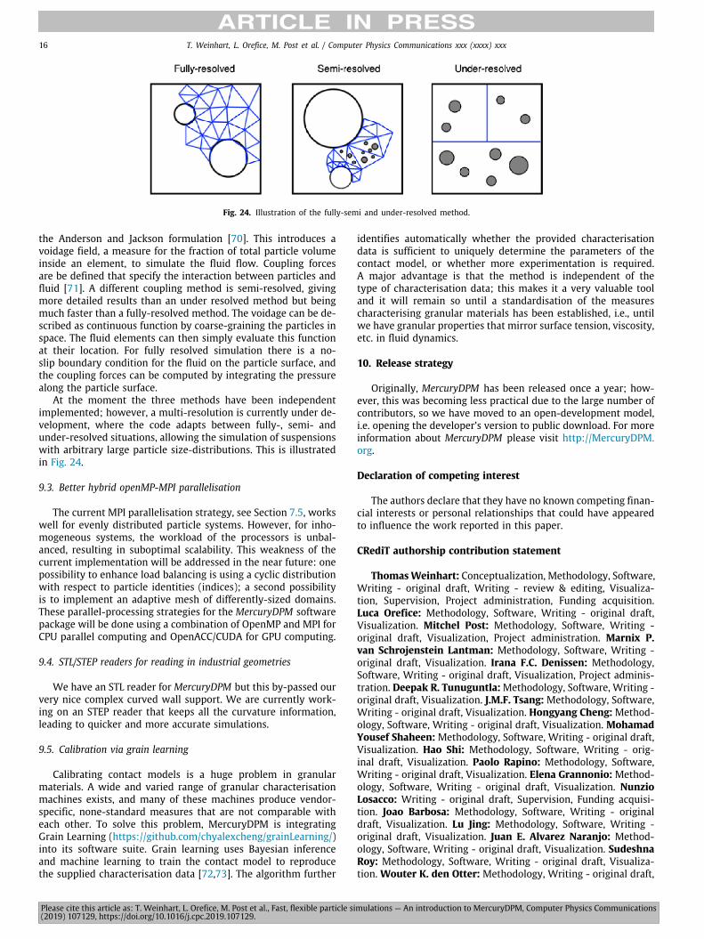
Please cite this article as: T. Weinhart, L. Orefice, M. Post et al., Fast, flexible particle simulations — An introduction to MercuryDPM, Computer Physics Communications(2019) 107129, https://doi.org/10.1016/j.cpc.2019.107129.
16 T. Weinhart, L. Orefice, M. Post et al. / Computer Physics Communications xxx (xxxx) xxx
Fig. 24. Illustration of the fully-semi and under-resolved method.
the Anderson and Jackson formulation [70]. This introduces avoidage field, a measure for the fraction of total particle volumeinside an element, to simulate the fluid flow. Coupling forcesare be defined that specify the interaction between particles andfluid [71]. A different coupling method is semi-resolved, givingmore detailed results than an under resolved method but beingmuch faster than a fully-resolved method. The voidage can be de-scribed as continuous function by coarse-graining the particles inspace. The fluid elements can then simply evaluate this functionat their location. For fully resolved simulation there is a no-slip boundary condition for the fluid on the particle surface, andthe coupling forces can be computed by integrating the pressurealong the particle surface.
At the moment the three methods have been independentimplemented; however, a multi-resolution is currently under de-velopment, where the code adapts between fully-, semi- andunder-resolved situations, allowing the simulation of suspensionswith arbitrary large particle size-distributions. This is illustratedin Fig. 24.
9.3. Better hybrid openMP-MPI parallelisation
The current MPI parallelisation strategy, see Section 7.5, workswell for evenly distributed particle systems. However, for inho-mogeneous systems, the workload of the processors is unbal-anced, resulting in suboptimal scalability. This weakness of thecurrent implementation will be addressed in the near future: onepossibility to enhance load balancing is using a cyclic distributionwith respect to particle identities (indices); a second possibilityis to implement an adaptive mesh of differently-sized domains.These parallel-processing strategies for the MercuryDPM softwarepackage will be done using a combination of OpenMP and MPI forCPU parallel computing and OpenACC/CUDA for GPU computing.
9.4. STL/STEP readers for reading in industrial geometries
We have an STL reader for MercuryDPM but this by-passed ourvery nice complex curved wall support. We are currently work-ing on an STEP reader that keeps all the curvature information,leading to quicker and more accurate simulations.
9.5. Calibration via grain learning
Calibrating contact models is a huge problem in granularmaterials. A wide and varied range of granular characterisationmachines exists, and many of these machines produce vendor-specific, none-standard measures that are not comparable witheach other. To solve this problem, MercuryDPM is integratingGrain Learning (https://github.com/chyalexcheng/grainLearning/)into its software suite. Grain learning uses Bayesian inferenceand machine learning to train the contact model to reproducethe supplied characterisation data [72,73]. The algorithm further
identifies automatically whether the provided characterisationdata is sufficient to uniquely determine the parameters of thecontact model, or whether more experimentation is required.A major advantage is that the method is independent of thetype of characterisation data; this makes it a very valuable tooland it will remain so until a standardisation of the measurescharacterising granular materials has been established, i.e., untilwe have granular properties that mirror surface tension, viscosity,etc. in fluid dynamics.
10. Release strategy
Originally, MercuryDPM has been released once a year; how-ever, this was becoming less practical due to the large number ofcontributors, so we have moved to an open-development model,i.e. opening the developer’s version to public download. For moreinformation about MercuryDPM please visit http://MercuryDPM.org.
Declaration of competing interest
The authors declare that they have no known competing finan-cial interests or personal relationships that could have appearedto influence the work reported in this paper.
CRediT authorship contribution statement
ThomasWeinhart: Conceptualization, Methodology, Software,Writing - original draft, Writing - review & editing, Visualiza-tion, Supervision, Project administration, Funding acquisition.Luca Orefice: Methodology, Software, Writing - original draft,Visualization. Mitchel Post: Methodology, Software, Writing -original draft, Visualization, Project administration. Marnix P.van Schrojenstein Lantman: Methodology, Software, Writing -original draft, Visualization. Irana F.C. Denissen: Methodology,Software, Writing - original draft, Visualization, Project adminis-tration. Deepak R. Tunuguntla:Methodology, Software, Writing -original draft, Visualization. J.M.F. Tsang: Methodology, Software,Writing - original draft, Visualization. Hongyang Cheng: Method-ology, Software, Writing - original draft, Visualization. MohamadYousef Shaheen: Methodology, Software, Writing - original draft,Visualization. Hao Shi: Methodology, Software, Writing - orig-inal draft, Visualization. Paolo Rapino: Methodology, Software,Writing - original draft, Visualization. Elena Grannonio: Method-ology, Software, Writing - original draft, Visualization. NunzioLosacco: Writing - original draft, Supervision, Funding acquisi-tion. Joao Barbosa: Methodology, Software, Writing - originaldraft, Visualization. Lu Jing: Methodology, Software, Writing -original draft, Visualization. Juan E. Alvarez Naranjo: Method-ology, Software, Writing - original draft, Visualization. SudeshnaRoy: Methodology, Software, Writing - original draft, Visualiza-tion. Wouter K. den Otter: Methodology, Writing - original draft,
Please cite this article as: T. Weinhart, L. Orefice, M. Post et al., Fast, flexible particle simulations — An introduction to MercuryDPM, Computer Physics Communications(2019) 107129, https://doi.org/10.1016/j.cpc.2019.107129.
T. Weinhart, L. Orefice, M. Post et al. / Computer Physics Communications xxx (xxxx) xxx 17
Funding acquisition. Anthony R. Thornton: Conceptualization,Methodology, Software, Writing - original draft, Writing - re-view & editing, Visualization, Supervision, Project administration,Funding acquisition.
Acknowledgements
The MercuryDPM team
MercuryDPM has been developed and tested by many peopleover the years and the code would not exist without the supportof all these people. Every time we develop a few new featureswe try and write a short conference proceeding giving credit toboth the people who developed these features and the peoplewho tested these features [2–4,35,74].
In addition to this we try to maintain a full list of contributorson the MercuryDPM website, see http://mercurydpm.org/about-the-code/team.
Funding
MercuryDPM would not exist without external funding and theauthors would like to acknowledge support from the followinggrants (since the project was started):
1. IMPACT-SIP1 ‘‘Computational multi-scale modelling ofsuper-dispersed multiphase flows’’
2. STW 11039 ‘‘Polydispersed Granular Flows through In-clined Channels’’
3. NWO VICI 10828 ‘‘Bridging the gap between particulatesystems and continuum theory’’;
4. DFG LU 450/10 ‘‘Sintering: modelling of pressure-,temperature-, or time-dependent contacts’’(part of SPP1482 ‘‘Partikel im Kontakt’’)
5. FOM 07PGM27 ‘‘Clustering phase diagram with dissipationand long range forces’’;
6. STW MuST 10120 ‘‘Molecular dynamics simulations ofgranular media’’
7. DFG-STW 12272 ‘‘Hydrodynamic theory of wet particlesystems’’
8. STW Take-Off Phase 1 ‘‘The MercuryLab Project’’9. STW VIDI 13472 ‘‘Shaping Segregation’’
10. STW 15050 ‘‘Multiscale modelling of agglomeration - Ap-plication to tableting and selective laser sintering’’
11. NWO VIDI 16604 ‘‘Virtual Prototyping of Particulate Pro-cesses’’
We would like to thank MercuryLab for their financial support,contribution to the code and the development of the trainingmaterial for MercuryDPM. MercuryLab is the official provider ofconsultancy, cloud interfaces and training for MercuryDPM andits associated tools. All MercuryLab training material is freelyavailable under the CC-BY licence.
References
[1] A.R. Thornton, D. Krijgsman, A. te Voortwis, V. Ogarko, S. Luding, R.Fransen, S. Gonzalez, O. Bokhove, O. Imole, T. Weinhart, Discrete Elem.Methods 6 (2013).
[2] A.R. Thornton, D. Krijgsman, R.H.A. Fransen, S.G. Briones, D.R. Tunuguntla,A. te Voortwis, S. Luding, O. Bokhove, T. Weinhart, EnginSoft Simul.-BasedEng. Sci. 10 (1) (2013) 48–53.
[3] T. Weinhart, D.R. Tunuguntla, M. van Schrojenstein-Lantman, A. van derHorn, I.F.C. Denissen, C.R. Windows-Yule, A.C. de Jong, A.R. Thornton, Proc.7th Int. Conf. Discrete Element Methods, Springer, 2016, pp. 1353–1360.
[4] T. Weinhart, D.R. Tunuguntla, M.P.V.S. Lantman, I.F. Denissen, C.R.W. Yule,H. Polman, J.M. Tsang, B. Jin, L. Orefice, K. van der Vaart, S. Roy, H. Shi,A. Pagano, W. den Breeijen, B. Scheper, A. Jarray, S. Luding, A.R. Thornton,Int. Conf. Particle-Based Methods V, 2017, pp. 123–134.
[5] P.A. Cundall, O.D.L. Strack, Géotechnique 29 (1) (1979) 47–65.[6] T. Pöschel, T. Schwager, Computational Granular Dynamics: Models and
Algorithms, Springer, 2005.[7] D. Palanisamy, Micro-Hydrodynamics of Non-
Spherical Colloids: a Brownian Dynamics Study(Ph.D. thesis), University of Twente, Enschede, The Netherlands, 2019.
[8] E. Anderson, Z. Bai, C. Bischof, S. Blackford, J. Demmel, J. Dongarra, J.Du Croz, A. Greenbaum, S. Hammarling, A. McKenney, D. Sorensen, LAPACKUsers’ Guide, third ed., Society for Industrial and Applied Mathematics,Philadelphia, PA, ISBN: 0-89871-447-8, 1999, (paperback).
[9] V. Ogarko, S. Luding, Comput. Phys. Comm. 183 (4) (2012) 931–936.[10] D. Krijgsman, V. Ogarko, S. Luding, Comput. Part. Mech. 1 (3) (2014)
357–372.[11] T. Weinhart, A.R. Thornton, S. Luding, O. Bokhove, Granul. Matter 14 (2)
(2012) 289–294.[12] T. Weinhart, R. Hartkamp, A.R. Thornton, S. Luding, Phys. Fluids 25 (7)
(2013) 070605.[13] D.R. Tunuguntla, A.R. Thornton, T. Weinhart, Comput. Part. Mech. 3 (3)
(2016) 349–365.[14] T. Weinhart, C. Labra, S. Luding, J.Y. Ooi, Powder Technol. 293 (2016)
138–148.[15] M.P. Allen, D.J. Tildesley, Computer Simulation of Liquids, Oxford University
Press, 1989.[16] A.R. Thornton, T. Weinhart, V. Ogarko, S. Luding, Comput. Methods Mater.
Sci. 13 (2) (2013) 197–212.[17] S. Raschdorf, M. Kolonko, Internat. J. Numer. Methods Engrg. 85 (2011)
625–639.[18] O.I. Imole, D. Krijgsman, T. Weinhart, V. Magnanimo, B.E.C. Montes, M.
Ramaioli, S. Luding, Powder Technol. 293 (2016) 69–81.[19] R. Kawamoto, E. Andò, G. Viggiani, J.E. Andrade, J. Mech. Phys. Solids 111
(2018) 375–392.[20] L. Piegl, W. Tiller, The NURBS Book, Springer, 2012.[21] J. Bel, D. Branque, H. Wong, G. Viggiani, N. Losacco, ITA-AITES World Tunnel
Congress 2016, WTC 2016, Vol. 4, 2016, pp. 3219–3229.[22] D.R. Tunuguntla, T. Weinhart, A.R. Thornton, Comput. Part. Mech. 4 (4)
(2017) 387–405.[23] S. Rubio-Largo, F. Alonso-Marroquin, T. Weinhart, S. Luding, R. Hidalgo,
Physica A 443 (2016) 477–485.[24] D. Tunuguntla, T. Weinhart, A. Thornton, Alert doctoral school 2017
discrete element modeling, 2017, p. 181.[25] S. Roy, B.J. Scheper, H. Polman, A.R. Thornton, D.R. Tunuguntla, S. Luding,
T. Weinhart, Eur. Phys. J. E 42 (2) (2019) 14.[26] K. van der Vaart, M. van Schrojenstein Lantman, T. Weinhart, S. Luding, C.
Ancey, A.R. Thornton, Phys. Rev. Fluids 3 (7) (2018) 074303.[27] H. Shi, S. Roy, T. Weinhart, V. Magnanimo, S. Luding, Granul. Matter 22
(14) (2020).[28] A. Lees, S. Edwards, J. Phys. C 5 (15) (1972) 1921.[29] D. Pan, J. Hu, X. Shao, Mol. Simul. 42 (4) (2016) 328–336.[30] H. Kobayashi, R. Yamamoto, J. Chem. Phys. 134 (6) (2011) 064110.[31] I.F.C. Denissen, T. Weinhart, A. Te Voortwis, S. Luding, J.M.N.T. Gray, A.R.
Thornton, J. Fluid Mech. 866 (2019) 263–297.[32] S. Luding, Granul. Matter 10 (4) (2008) 235.[33] J. Tomas, Powder Handl. Process. 15 (5) (2003) 296–314.[34] R. Fuchs, T. Weinhart, M. Ye, S. Luding, H.-J. Butt, M. Kappl, EPJ Web of
Conferences, Vol. 140, EDP Sciences, 2017, p. 13012.[35] T. Weinhart, M. Post, I.F.C. Denissen, D.R. Tunuguntla, E. Grannonio, N.
Losacco, J.M.F. Tsang, J. Barbosa, W. den Otter, A.R. Thornton, 8th Int. Conf.Discrete Element Methods, Springer, 2019.
[36] S. Roy, A. Singh, S. Luding, T. Weinhart, Comput. Part. Mech. 3 (4) (2016)449–462.
[37] S. Roy, S. Luding, T. Weinhart, Phys. Rev. E 98 (5) (2018) 052906.[38] A.G. Pagano, V. Magnanimo, T. Weinhart, A. Tarantino, Géotechnique, 0,
(0) 1, https://doi.org/10.1680/jgeot.18.P.060.[39] Tribology-ABC, Hertzian contacts, 2015, http://www.tribology-abc.com/
sub10.htm, [Online; accessed 01 August 2015].[40] C. Thornton, J. Appl. Mech. 64 (2) (1997) 383–386.[41] S. Luding, Phys. Dry Granul. Media - NATO ASI Ser. E350 (ISSN: 0168-132X)
1 (1998) 285.[42] R.L. Jackson, I. Green, D.B. Marghitu, Nonlinear Dynam. 60 (3) (2010)
217–229.[43] C. Thornton, S.J. Cummins, P.W. Cleary, Powder Technol. 233 (2013) 30–46.[44] E.R. Johnston, Vector Mechanics for Engineers: Statics and Dynamics, Vol.
1, Tata McGraw-Hill Education, 2009.[45] O.R. Walton, R.L. Braun, J. Rheol. (1978-present) 30 (5) (1986) 949–980.[46] O.R. Walton, Mech. Mater. 16 (1) (1993) 239–247.[47] J. Blendell, Encyclopedia of Materials: Science and Technology, Elsevier,
Oxford, ISBN: 978-0-08-043152-9, 2001, pp. 8745–8750.[48] T. Weinhart, R. Fuchs, T. Staedler, M. Kappl, S. Luding, Particles in Contact:
Micro Mechanics, Micro Process Dynamics and Particle Collective, Springer,2019, pp. 311–338.
Please cite this article as: T. Weinhart, L. Orefice, M. Post et al., Fast, flexible particle simulations — An introduction to MercuryDPM, Computer Physics Communications(2019) 107129, https://doi.org/10.1016/j.cpc.2019.107129.
18 T. Weinhart, L. Orefice, M. Post et al. / Computer Physics Communications xxx (xxxx) xxx
[49] R. Fuchs, T. Weinhart, J. Meyer, H. Zhuang, T. Staedler, X. Jiang, S. Luding,MRS Proc. 1652 (2014) mrsf13–1652–ll07–07.
[50] R. Fuchs, M. Ye, T. Weinhart, S. Luding, H.-J. Butt, M. Kappl, InternationalCongress on Particle Technology (ParTec), 2016.
[51] M.Y. Shaheen, A.R. Thornton, S. Luding, T. Weinhart, Int. Conf. DiscreteElement Methods (DEM8), 2019.
[52] Y. Gan, P. Rognon, I. Einav, Phil. Mag. 92 (28–30) (2012) 3405–3417.[53] R. Fuchs, J. Meyer, T. Staedler, X. Jiang, Tribol. - Mater. Surf. Interfaces 7
(2) (2013) 103–107.[54] S. Roy, S. Luding, T. Weinhart, New J. Phys. 19 (4) (2017) 043014.[55] C.D. Willett, M.J. Adams, S.A. Johnson, J.P. Seville, Langmuir 16 (24) (2000)
9396–9405.[56] S. Roy, S. Luding, W.K. den Otter, A.R. Thornton, T. Weinhart, J. Fluid Mech.
(2019) submitted for publication.[57] R. Hibbeler, Engineering Mechanics: Statics & Dynamics, 14th Edn.
Hoboken, Pearson Prentice Hall Pearson Education, Inc, NJ, 2016.[58] A. Podlozhnyuk, S. Pirker, C. Kloss, Comput. Part. Mech. 4 (1) (2017)
101–118.[59] I.F.C. Denissen, On Segregation in Bidisperse Granular Flows
(Ph.D. thesis), University of Twente, Enschede, The Netherlands, 2019.[60] S. He, J. Gan, D. Pinson, Z. Zhou, Powder Technol. 341 (2019) 157–166.[61] R. Furukawa, K. Kadota, T. Noguchi, A. Shimosaka, Y. Shirakawa, AAPS
Pharm. Sci. Tech. 18 (6) (2017) 2368–2377.
[62] A. Skelbæk-Pedersen, T. Vilhelmsen, V. Wallaert, J. Rantanen, J. Pharm. Sci.108 (3) (2019) 1246–1253.
[63] D. Mašín, Eng. Geol. 165 (2013) 73–88.[64] M.P. van Schrojenstein Lantman, A Study on Fundamen-
tal Segregation Mechanisms in Dense Granular Flows(Ph.D. thesis), University of Twente, Enschede, The Netherlands, 2019.
[65] M. Heil, A.L. Hazel, Fluid-Structure Interaction, Springer, 2006, pp. 19–49.[66] M. Dratt, A. Katterfeld, Granul. Matter 19 (3) (2017) 49.[67] G. Ma, W. Zhou, X.-L. Chang, W. Yuan, Int. J. Geomech. 14 (4) (2013)
04014014.[68] H. Cheng, H. Yamamoto, K. Thoeni, Y. Wu, Geotext. Geomembr. 45 (4)
(2017) 361–376.[69] H. Cheng, H. Yamamoto, N. Guo, H. Huang, Proc. 7th Int. Conf. Discrete
Element Methods, Springer Singapore, Singapore, 2017, pp. 445–453.[70] T. Anderson, R. Jackson, Ind. Eng. Chem. Fundam. 6 (4) (1967) 527–539.[71] C. Davies, J. Aerosol Sci. 10 (5) (1979) 477–513.[72] H. Cheng, T. Shuku, K. Thoeni, H. Yamamoto, Granul. Matter 20 (1) (2018)
11.[73] H. Cheng, T. Shuku, K. Thoeni, P. Tempone, S. Luding, V. Magnanimo,
Comput. Methods Appl. Mech. Engrg. 350 (2019) 268–294.[74] A.R. Thornton, M. Post, L. Orefice, P. Rapino, S. Roy, H. Polman, M.Y.
Shaheen, J. Alvarez Naranjo, H. Cheng, L. Jing, H. Shi, J. Mbaziira, R. Roeplal,T. Weinhart, 8th Int. Conf. Discrete Element Methods, Springer, 2019.
Related Documents