Fast estimators of time delay and Doppler stretch based on discrete-time methods

IEEE TRANSACTIONS ON SIGNAL PROCESSING, VOL. 46, NO. 7, JULY 1998 1785

Fast Estimators of Time Delay and DopplerStretch Based on Discrete-Time Methods

Gaetano Giunta,Member, IEEE

Abstract—Estimation of the time delay and the Doppler stretchof a signal is required in several signal processing applications.This paper is focused on joint fine estimation of these twoparameters by a fast interpolation of the estimated ambiguityfunction. Four discrete-time methods (viz. multirate, piecewisescaling, linear scaling, and indirect estimators), based on anorthogonal model, are introduced. Their mean square error ismathematically derived for random signals corrupted by additiverandom noises. The obtained expressions have been evaluated forsome typical parameter sets in the reference case of Gaussiansignal and noises. The numerical results, compared with theaccuracy of a continuous-time estimator, show the near efficiencyof the multirate estimator for a wide range of SNR’s. In fact, theadjustable multirate estimator can operate under near optimalconditions, unlike the approximate (i.e., piecewise and linear)scaling and the indirect methods based on constant samplingrates.

I. INTRODUCTION

JOINT estimation of time delay and Doppler stretch of asignal is required in many signal processing applications.

Among them, we can mention estimation of direction-of-arrival and range in multisensor arrays, RF communications,spread spectrum mobile communications, motion compensa-tion in moving images, stereo vision, profiling in telesensingsystems, moving object recognition and tracking, ultrasonicechography, etc.

The interest in time-delay estimation has moved from theinitial area of underwater acoustics. In particular, digital meth-ods for delay and Doppler fast estimation are very important indigital communication systems, in the presence of motion, andin recent applications to mobile communications. Fast algo-rithms for motion estimation and compensation are widely ad-dressed in image processing and computer vision applications.In addition, basic topics such as spectral estimation and mul-tiple parameter estimation have a relevant theoretical interest.

Estimation of the Doppler coefficient from narrowbandsignals consists of evaluating the shift of the center frequencyfrom the instantaneous signal spectrum [1]. Wideband signalsare conversely required to improve the spatial resolution ofan imaging system. The dominant effect of relative motionconsists of a time scaling of the received signal. If a complexsignal representation is employed, its baseband equivalent isalso multiplied by a complex exponential whose frequencyinvolves both the Doppler coefficient and the carrier or center

Manuscript received January 7, 1996; revised December 3, 1997. Theassociate editor coordinating the review of this paper and approving it forpublication was Prof. Victor A. N. Barroso.

The author is with the INFO-COM Department, University of Rome “LaSapienza,” Rome, Italy (e-mail: [email protected]).

Publisher Item Identifier S 1053-587X(98)04416-X.

frequency. Simultaneous estimation of time-delay and Dopplercoefficient is based on the minimization of a two-dimensional(2-D) ambiguity function, according to the maximum likeli-hood (ML) criterion [2]–[5].

Previous papers did not explicitly use discrete-time rep-resentations but extensively reported the results of computersimulations, such as a lot of papers in a seminal book edited byCarter [6]. In fact, continuous-time implementation of Dopplertime scaling is quite complex and expensive. Moreover, allthe possible Doppler scaling factor should be considered inthe ML procedure. An indirect continuous estimator, based onone-dimensional (1-D) estimates of the time-varying delaysbetween a set of time-space partitions of the array data, wasdevised in [7] to reduce the computational loading in the caseof high signal-to-noise ratio (SNR). A continuous-time time-scaling method, based on preliminary short-time correlograms,progressively shifted and added, was suggested by Betz [8]. Heanalyzed the effect on the cross-correlation function (CCF) ofa piecewise constant approximation of a linearly time-varyingdelay (see also [9]).

Digital processing techniques, based on fast interpolationof some estimated ambiguity samples, are particularly suitedfor real-time estimation of signal parameters to reduce thetremendous computational cost of a 2-D processing. Fastdiscrete-time CCF techniques (viz. the conventional multiply-and-add (M&A), the average magnitude difference function(AMDF), and the average square difference function (ASDF)estimators) were devised and analyzed in [10] for a constanttime delay (i.e., with no Doppler stretch). They are based onparabolic interpolation of the sampled CCF or cross ambiguity.Such a fast technique is widely used in practice. Time-delayestimation results quite different in the presence of movingsource or receivers since time-varying correlation is requiredin such cases [2]–[3].

A two-dwell system for timing and Doppler acquisition inspread-spectrum communications was analyzed in [11] in thecase of bandpass wideband signals. Both the Doppler effectson the complex model (i.e., the Doppler shift of the centerfrequency and the Doppler stretch of the baseband signalequivalents) were therein addressed. The devised method isbased on sequential alternate estimates of one parameter at atime selected over a 2-D uncertainty region on a discrete set oftrial values. The authors of [11] also discussed how to performa closed-loop system for an effective tracking at the end of asuccessful acquisition.

This paper is focused on joint fine estimation of time delayand Doppler coefficient by a fast interpolation of the estimatedambiguity function. Some preliminary results of computer

1053–587X/98$10.00 1998 IEEE

1786 IEEE TRANSACTIONS ON SIGNAL PROCESSING, VOL. 46, NO. 7, JULY 1998

simulations were presented by the author in [12]. The use offast techniques is required when the radial acceleration is notnegligible. In such a case, a large number of estimates can becollected during the whole observation window.

A set of fast discrete-time algorithms (namely, multirate,piecewise-scaling, linear scaling, and indirect estimators) is de-vised in this paper for fine estimation of these two parameters.Their performance is investigated by an approximate analysisof the bias and error variance based on a Taylor’s series expan-sion in the CCF samples. In particular, mathematical expres-sions are derived as parametric functions. The results of com-puter simulations corroborate the obtained analytical results.

II. DOPPLER MODEL AND ESTIMATION

Let us refer to the following model of the signals andreceived by two sensors:

(1)

(2)

where is a gain factor, whereas the noises andare uncorrelated with each other and with the signal

. Both real and complex notation may be employed torepresent the useful signal, the two noises, and the gain factor,by using the baseband equivalents of the bandpass signals withrespect to the center frequency ( in the real case).

The problem we address is accurate time delay and Dopplerstretch estimation (i.e., the parametersand , respectively).Such an estimation is particularly effective when it operates onwidebandsignals. It should be carried out by a 2-D matchingbetween the observed portion of the reference signaland all the shifted (by the delay) and time stretched (bythe time-scaling factor ) amplitude-compensated versions

, which are derived from thetime-scaled versions of the received signal . A consistentmethod converges to the estimates: and .

Many previous papers formulated the problem to (approx-imately or exactly) eliminate the coupling between the twoestimates. Two equivalent models were used in the literaturefor a Doppler-stretched received signal (letting againin the real case), i.e.,

(3)

(4)

Let the reference signal be observed for; the CCF estimated from and presents

a maximum satisfying one of the following statisticalconditions (if a consistent estimator is employed):

for (2):

for (3):

for (4):

(5)

It can be observed that the choice makes theestimates of and uncorrelated for the models (2) and (4).In such a case, the mean estimated delay is for anyvalue of . The models (4) (employed in [2]) and (2) (used

in [5] and here) are suited for a separate estimation ofand. In fact, they do not present a coupling (i.e., a correlation

between the estimates) between the two parameters for anyvalue of . The authors employing the model (3) ([3], [4], [7],[8], [9], [11]) assumed that to approximately avoid theproblem of joint estimation of correlated parameters. In fact,a systematic bias (i.e., ) affects the estimate of.

The joint statistics of the observed data in (1) and (2)–(4) areinherently nonstationary whenis not zero. In fact, the meandelay of two partitions of the received signals linearly dependson the current time. Moreover, the statistical CCF vanishesfor increasing observation windows. As a consequence, short-time signal partitions, compared with the width of the signalautocorrelation function (ACF), must be considered to allowan effective estimation of the mean delay of that partition. Itmust be observed that such a partitioning should be symmetricaround to obtain orthogonal estimates ofand [forthe models (2) and (4)] after averaging over all the consideredblocks (see also Section IV-D).

The ML criterion is based on the minimization of the Eu-clidean distance between the reference signal and a num-ber of time-stretched versions of the amplitude-compensatedreceived signal . It should be noted that the complexexponential may be synthetically implemented. In fact, it onlydepends on the center frequency and the trial values of delayand Doppler coefficients.

Since we are dealing with bandlimited signals, let us con-sider the following discrete-time M&A, ASDF, and AMDFcorrelators working on the processes and :

(6)

(7)

(8)

letting:

where and are the sampling intervals of thesignals and , all of them assumed to satisfythe Nyquist’s conditions, whereas the observation windows

for andfor are considered.

The time delay and Doppler stretch estimates are, for allthe three correlators (6)–(8)

(9)

GIUNTA: FAST ESTIMATORS OF TIME DELAY AND DOPPLER STRETCH BASED ON DISCRETE-TIME METHODS 1787

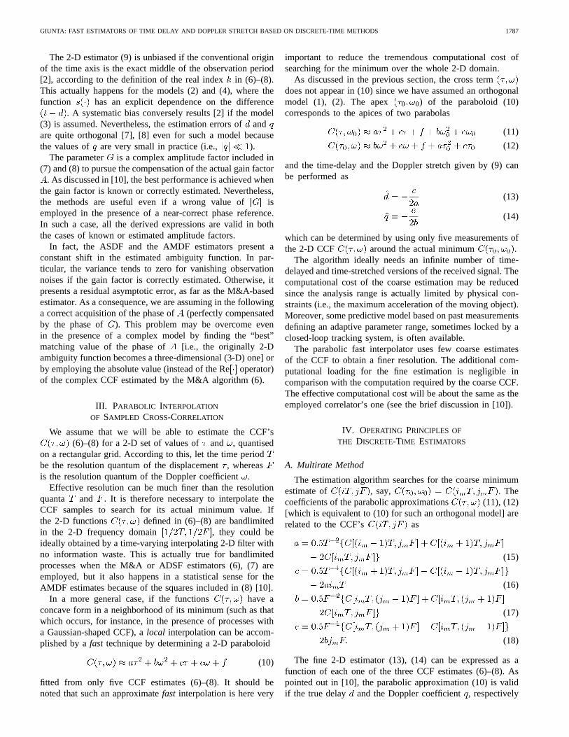
The 2-D estimator (9) is unbiased if the conventional originof the time axis is the exact middle of the observation period[2], according to the definition of the real indexin (6)–(8).This actually happens for the models (2) and (4), where thefunction has an explicit dependence on the difference

. A systematic bias conversely results [2] if the model(3) is assumed. Nevertheless, the estimation errors ofandare quite orthogonal [7], [8] even for such a model becausethe values of are very small in practice (i.e., ).

The parameter is a complex amplitude factor included in(7) and (8) to pursue the compensation of the actual gain factor

. As discussed in [10], the best performance is achieved whenthe gain factor is known or correctly estimated. Nevertheless,the methods are useful even if a wrong value of isemployed in the presence of a near-correct phase reference.In such a case, all the derived expressions are valid in boththe cases of known or estimated amplitude factors.

In fact, the ASDF and the AMDF estimators present aconstant shift in the estimated ambiguity function. In par-ticular, the variance tends to zero for vanishing observationnoises if the gain factor is correctly estimated. Otherwise, itpresents a residual asymptotic error, as far as the M&A-basedestimator. As a consequence, we are assuming in the followinga correct acquisition of the phase of(perfectly compensatedby the phase of ). This problem may be overcome evenin the presence of a complex model by finding the “best”matching value of the phase of [i.e., the originally 2-Dambiguity function becomes a three-dimensional (3-D) one] orby employing the absolute value (instead of the Reoperator)of the complex CCF estimated by the M&A algorithm (6).

III. PARABOLIC INTERPOLATION

OF SAMPLED CROSS-CORRELATION

We assume that we will be able to estimate the CCF’s(6)–(8) for a 2-D set of values of and , quantised

on a rectangular grid. According to this, let the time periodbe the resolution quantum of the displacement, whereasis the resolution quantum of the Doppler coefficient.

Effective resolution can be much finer than the resolutionquanta and . It is therefore necessary to interpolate theCCF samples to search for its actual minimum value. Ifthe 2-D functions defined in (6)–(8) are bandlimitedin the 2-D frequency domain , they could beideally obtained by a time-varying interpolating 2-D filter withno information waste. This is actually true for bandlimitedprocesses when the M&A or ADSF estimators (6), (7) areemployed, but it also happens in a statistical sense for theAMDF estimates because of the squares included in (8) [10].

In a more general case, if the functions have aconcave form in a neighborhood of its minimum (such as thatwhich occurs, for instance, in the presence of processes witha Gaussian-shaped CCF), alocal interpolation can be accom-plished by afast technique by determining a 2-D paraboloid

(10)

fitted from only five CCF estimates (6)–(8). It should benoted that such an approximatefast interpolation is here very

important to reduce the tremendous computational cost ofsearching for the minimum over the whole 2-D domain.

As discussed in the previous section, the cross termdoes not appear in (10) since we have assumed an orthogonalmodel (1), (2). The apex ) of the paraboloid (10)corresponds to the apices of two parabolas

(11)

(12)

and the time-delay and the Doppler stretch given by (9) canbe performed as

(13)

(14)

which can be determined by using only five measurements ofthe 2-D CCF around the actual minimum .

The algorithm ideally needs an infinite number of time-delayed and time-stretched versions of the received signal. Thecomputational cost of the coarse estimation may be reducedsince the analysis range is actually limited by physical con-straints (i.e., the maximum acceleration of the moving object).Moreover, some predictive model based on past measurementsdefining an adaptive parameter range, sometimes locked by aclosed-loop tracking system, is often available.

The parabolic fast interpolator uses few coarse estimatesof the CCF to obtain a finer resolution. The additional com-putational loading for the fine estimation is negligible incomparison with the computation required by the coarse CCF.The effective computational cost will be about the same as theemployed correlator’s one (see the brief discussion in [10]).

IV. OPERATING PRINCIPLES OF

THE DISCRETE-TIME ESTIMATORS

A. Multirate Method

The estimation algorithm searches for the coarse minimumestimate of , say, . Thecoefficients of the parabolic approximations (11), (12)[which is equivalent to (10) for such an orthogonal model] arerelated to the CCF’s as

(15)

(16)

(17)

(18)

The fine 2-D estimator (13), (14) can be expressed as afunction of each one of the three CCF estimates (6)–(8). Aspointed out in [10], the parabolic approximation (10) is validif the true delay and the Doppler coefficient, respectively


lie within and[see (19) and (20) at the bottom of the page].

The algorithm for fine estimation requires to generate anumber of time-stretched versions of the received signal.This step needs a perfect scaling of the time axis for eachconsidered Doppler coefficient. This may be implemented bya sampling rate change of the received signal (and a propermodulation in the complex case) according (6)–(8). Thesampling rate may be also adaptively adjusted as suggestedby [2]. In practice, only three Doppler values are necessaryfor several applications [11].

B. Piecewise-Scaling Method

The Doppler effect is equivalent to a time-varying delayof the received signal, with respect to the reference one.If we approximate the linear delay by a piecewise constantfunction, this is equivalent to an increasing piecewise function.Such azero-order approximationwas first suggested by Betz[8], [9] in order to reduce the computational complexity ofimplementing Doppler time scaling. He devised a continuous-time estimation algorithm in which the CCF estimates fromsmall blocks of unstretched received data are progressivelyshifted and added. The “best” speed of the increasing time-delay corresponds to the Doppler coefficient estimate.

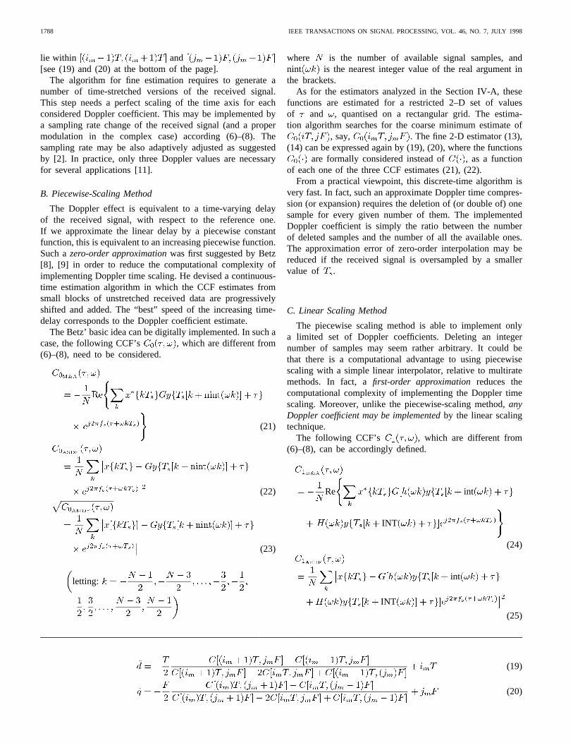
The Betz’ basic idea can be digitally implemented. In such acase, the following CCF’s , which are different from(6)–(8), need to be considered.

(21)

(22)

(23)

letting:

where is the number of available signal samples, andnint is the nearest integer value of the real argument inthe brackets.

As for the estimators analyzed in the Section IV-A, thesefunctions are estimated for a restricted 2–D set of valuesof and , quantised on a rectangular grid. The estima-tion algorithm searches for the coarse minimum estimate of

, say, . The fine 2-D estimator (13),(14) can be expressed again by (19), (20), where the functions

are formally considered instead of , as a functionof each one of the three CCF estimates (21), (22).

From a practical viewpoint, this discrete-time algorithm isvery fast. In fact, such an approximate Doppler time compres-sion (or expansion) requires the deletion of (or double of) onesample for every given number of them. The implementedDoppler coefficient is simply the ratio between the numberof deleted samples and the number of all the available ones.The approximation error of zero-order interpolation may bereduced if the received signal is oversampled by a smallervalue of .

C. Linear Scaling Method

The piecewise scaling method is able to implement onlya limited set of Doppler coefficients. Deleting an integernumber of samples may seem rather arbitrary. It could bethat there is a computational advantage to using piecewisescaling with a simple linear interpolator, relative to multiratemethods. In fact, afirst-order approximationreduces thecomputational complexity of implementing the Doppler timescaling. Moreover, unlike the piecewise-scaling method,anyDoppler coefficient may be implementedby the linear scalingtechnique.

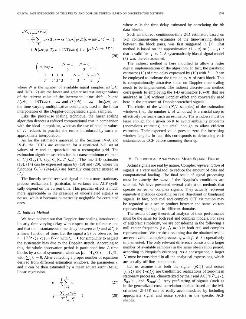
The following CCF’s , which are different from(6)–(8), can be accordingly defined.

Re int

INT

(24)

int

INT

(25)

(19)

(20)


int

INT

(26)

letting:

where is the number of available signal samples, intand INT are the lower and greater nearest integer valuesof the current value of the incremental time shift , and

and arethe time-varying multiplicative coefficients used in the linearinterpolation of the Doppler-compensated signal samples.

Like the piecewise scaling technique, the linear scalingalgorithm denotes a reduced computational cost in comparisonwith the ideal interpolator, whereas the use of smaller valuesof reduces in practice the errors introduced by such anapproximate interpolation.

As for the estimators analyzed in the Sections IV-A andIV-B, the CCF’s are estimated for a restricted 2-D set ofvalues of and , quantized on a rectangular grid. Theestimation algorithm searches for the coarse minimum estimateof , say, . The fine 2-D estimator(13), (14) can be expressed again by (19) and (20), where thefunctions (24)–(26) are formally considered instead of

.The linearly scaled received signal is not a more stationary

process realization. In particular, its variance and ACF cycli-cally depend on the current time. This peculiar effect is muchmore appreciable in the presence of uncorrelated signals ornoises, while it becomes numerically negligible for correlatedones.

D. Indirect Method

We have pointed out that Doppler time scaling introduces alinearly time-varying delay with respect to the reference oneand that the instantaneous time delay between and isa linear function of time. Let the signal be observed for

, with for simplicity to neglectthe systematic bias due to the Doppler stretch. According tothis, the whole observation period is partitioned intotimeblocks by a set of symmetric windows ,with . After collecting a proper number of equationsderived from different estimation windows, the parametersand can be then estimated by a mean square error (MSE)linear regression

(27)

(28)

where is the time delay estimated by correlating thethdata blocks.

Such an indirect continuous-time 2-D estimator, based on1-D continuous-time estimates of the time-varying delaysbetween the block pairs, was first suggested in [7]. Thatmethod is based on the approximationthat is valid for . A systematically biased signal model(3) was therein assumed.

The indirect method is here modified to allow a fasterdigital implementation of the algorithm. In fact, the parabolicestimator (13) of time delay expressed by (19) with canbe employed to estimate the time delayof each block. Thisis computationally attractive since no Doppler time-scalingneeds to be implemented. The indirect discrete-time methodcorresponds to employing the 1-D estimators (6)–(8) that areanalyzed in [10] without Doppler effect and conversely usedhere in the presence of Doppler-stretched signals.

The choice of the width ( samples) of the estimationwindows (i.e., the number of windows) is a crucial step toeffectively performe such an estimator. The windows must belarge enough for a given SNR to avoid ambiguity problems(anomalous estimates) but small enough to allow efficientestimates. Their expected value goes to zero for increasingwindow lengths. In fact, this corresponds to defocusing eachinstantaneous CCF before summing them up.

V. THEORETICAL ANALYSIS OF MEAN SQUARE ERROR

Actual signals are real by nature. Complexrepresentationofsignals is a very useful tool to reduce the amount of data andcomputational loading. The final result of signal processingmust be exactly the sameif the Nyquist’s conditions aresatisfied. We have presented several estimation methods thatoperate on real or complex signals. They actually representequivalentmethods operating on real (baseband or bandpass)signals. In fact, both real and complex CCF estimation maybe regarded as a scalar product between the same vectorsrepresenting the signal in different domains.

The results of any theoretical analysis of their performancemust be the same for both real and complex models. For sakeof algebraic simplicity, we are considering in the following anull center frequency (i.e. ) in both real and complexrepresentations. We are then assuming that the obtained resultsare even valid if complex processing with is operativelyimplemented. The only relevant difference consists of a largernumber of available samples (in the same observation period,according to Nyquist’s criterion). As a consequence, a larger

must be considered in all the analytical expressions, whichare usually off-line computated.

Let us assume that both the signal and noisesand are bandlimited realizations of zero-mean

stationary processes, characterized by their real ACF’s ,, and . Any prefiltering of signals (such as

in the generalized cross-correlation method based on the MLcriterion [2]–[5]) can be easily accommodated by includingappropriate signal and noise spectra in the specific ACFshapes.


A. Basic Definitions and General Guidelines

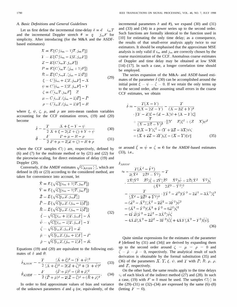
Let us first define the incremental time-delayand the incremental Doppler stretch forsimplicity. After introducing (for the M&A and the ASDF-based estimators)

(29)

where and are zero-mean random variablesaccounting for the CCF estimation errors, (19) and (20)become

(30)

(31)

where the CCF samples are, respectively, defined by(6) and (7) for the multirate method or by (21) and (22) forthe piecewise-scaling, for direct estimation of delay (19) andDoppler (20).

Conversely, if the AMDF estimates , which aredefined in (8) or (23) according to the considered method, aretaken for convenience into account, let

(32)

Equations (19) and (20) are equivalent to the following esti-mates of and :

(33)

(34)

In order to find approximate values of bias and varianceof the unknown parameters and (or, equivalently, of the

incremental parameters and ), we expand (30) and (31)and (33) and (34) in a power series up to the second order.Such functions are formally identical to the function used in[10] for estimating the only time delay; as a consequence,the results of that small-error analysis apply twice to ourestimators. It should be emphasised that the approximate MSEanalysis is only valid if and are correctly chosen by thecoarse maximization of the CCF. Anomalous coarse estimatesof Doppler and time delay may be obtained at low SNR[14]–[17]. In such a case, a longer correlation time shouldbe employed.

The series expansion of the M&A- and ASDF-based esti-mates of the parameter(30) can be accomplished around theinitial point . If we retain the only terms upto the second order, after assuming small errors in the coarseCCF estimates, we obtain

(35)

or around for the AMDF-based estimates(33), i.e.,

(36)

Quite similar expressions for the estimates of the parameter[defined by (31) and (34)] are derived by expanding them

up to the second order around and, respectively. The analytical result of such

derivation is obtainable by the formal substitution (35) and(36) of the parameters and withand respectively.

On the other hand, the same results apply to the time delaysof each block of the indirect method (27) and (28). In such

a case, (19) with must be used. The samples inthe (29)–(31) or (32)–(34) are expressed by the same (6)–(8)(letting ).


B. Framework of the Bias and Variance Expressions

The bias and the error variance of the estimates of theunknown parameters and depend on the variances andthe cross-covariances of the zero-mean random variables ac-counting for the CCF estimation errors (whose statistics willbe reported in the following subsection). In particular, the biasdepends on the even terms of the Taylor’s series approxi-mations (35), (36), whereas the odd terms are involved inthe approximate expressions of the error variance. The biasdirectly comes from a statistical expectation, whereas only thecross products of the linear coefficients affect the varianceexpression after retaining the terms up to the second order.

If the M&A and the ASDF correlators are employed, thebias of the multirate and piecewise-scaling direct estimate ofthe time delay results:

bias

var var

var cov

cov cov

(37)

while the estimation variance is

var cov

cov

cov var

var var (38)

If the AMDF correlator is used, the bias has the followingexpression:

bias

var

var

var

cov

cov

cov (39)

and its estimation variance assumes the form

var

cov

cov

cov

var var

var (40)

The first two terms in (37) and (39) represent themisfit ofthe true ACF with the parabolic approximation and dependon the actual signal ACF. Thissystematic biasis independent

of the observation window but can be easily predicted if theactual power spectra are known [10], [13].

The generic expressions of the accuracy are quite cum-bersome for a comparative performance discussion. Simplermathematical expressions of bias and error variance are de-rived by assuming that the central samples of the coarseestimates are in the neighborhood of their actual values. Thiscondition may happen, for instance, in a closed-loop trackingsystem or after an accurate pre-estimation using adjustablesampling rates.

Some symmetries hold under this assumption. In particular,it happens that var var varvar cov cov , and cov cov . Asa consequence, the bias goes to zero since , whereas thevariance expression of the estimates offor the M&A andASDF correlators (38) simplifies as

var var cov (41)

whereas (40), which is valid for the AMDF estimator, reducesto

var var cov

(42)

Both the general and the simplified expressions of the biasand the variance of the incremental Doppler parametercan beobtained by the formal substitution in all the above equationsof the parameters and with and ,respectively, for all the estimators considered in this paper.

The bias and the variance of the indirect method can beapproximately evaluated by assuming the statistical indepen-dence of all the blocks of data. In fact, the estimateddelay and Doppler coefficient are linear combinations of theincremental time delays of each block according to (27) and(28). Under this assumption, it trivially follows that

bias bias (43)

var var (44)

biasbias

(45)

varvar

(46)

C. Derivation of Explicit Mean and CovarianceExpressions for Gaussian Processes

Accuracy depends on signal and noise statistics. In orderto evaluate it in a closed form, let us assume that bothsignal and noises are realizations of zero-mean Gaussianrandom processes or, at least, that theirfourth-order momentsfactor like Gaussian. Accuracy therefore depends on mean andACF’s only.

Unlike the real ACF’s of baseband signal and noises, theeffective bandpass ACF’s are rotated in the presence of aphase reference error. In such a case, the term AG is not


more a real factor, and the complex analytic ACF’s (i.e.,evaluated for and involving their Hilbert transform)must be considered in all the following expressions insteadof the real ACF’s. In many practical applications (see [11]),such a problem is avoided if the absolute value (instead of theRe operator) of the complex M&A estimator is taken intoaccount to demodulate the signals by anoncoherenttechnique,approximating acoherentdemodulation for high SNR.

The mean values, the variance, and the cross covarianceshere considered have different forms from the ones reportedin [10] since Doppler affects the received signal (2). The meanvalues are functions of the variables and ,whereas the covariances depend on thevariables and . All the expressions required inthe Section V-B are obtained by substituting proper values tothe variables and .

Let us define, for convenience

Re (47)

(48)

By rearranging known results about second- and fourth-ordermoments of Gaussian processes, we obtain, after some ma-nipulations

Re (49)

Cov

Re

(50)

(51)

(52)

with for the real case and for the complexone in (52) and (53), while it results, for the AMDF-basedestimator in

(53)

Cov

(54)

with baseband signals, whereas the above expressions become,in the complex case:

(55)

Cov

(56)

where is theGaussian hypergeometric function,which is defined as [20], [21]

(57)

letting:

It can be observed that all the error covariances are roughlyproportional to the term . In fact, only the indices

in the double sums will remain for the ideal caseof independent pairs of uncorrelated samples for

and under the assumption thatthe estimates are distributed in the small error regime.

Equations (47)–(56) directly apply to the multirate directestimator and to the indirect method (with ),based on the correlators (6)–(8). The relationships of the meansand the covariances for the piecewise-scaling technique can betrivially derived in the same way. In particular, the piecewise-scaling algorithm, which employs the correlators (21)–(23),has performance predicted by the same expressions (47)–(56),where all the terms are substituted bynint nint nint , respectively.


The accuracy of the linear scaling method can be converselyderived after a proper manipulation of the same (47)–(56).The expressions containing the ACF’s of the signal andof the received noise depend on the current time. Inparticular, they are modified by substituting the generic ACF

, depending on the product (or, equivalently,or ) and some further parameters, with a term

coming from the linear interpolation of the received signal

int INT

and the ACF , depending on the two prod-ucts and and some further parameters, with theterm coming from the cross products between the samples ofthe linearly interpolated received signal

int

int INT

int

INT INT

where the same definitions as in the Section IV-C have beenemployed. Moreover, the dependence on the current time ofthe signal and noise variances in the linear scaling methodalso affects (47) as

Reint

INT(58)

D. Remarks on the Accuracy with Non-Gaussian Signals

The accuracy of the devised methods has been evaluated byimplicit expressions as a function of the four-fold moments ofthe random variables involved in the cross-correlation estima-tion. If the statistical distribution of such random variables isknown, the estimation accuracy can be expressed in an explicitform.

The expressions of the Section V.D have been derivedunder the assumption of signal fourth moments that factorlike Gaussian. The authors of [5] claimed a different behaviorbetween the Gaussian and the non-Gaussian cases with refer-ence to theshapeof the signal pulses but did not analyze thecase of differentprobability density functions. The expressionsreported in this paper statistically account for the particularsignal waveform by its ACF.

In fact, the assumption of signal (or signal difference)fourth moments that factor like Gaussian can be often made(even in the non-Gaussian case) for the following reasons.First, a statistical distribution models a collection of randomrealizations. It refers to theirensemble(not temporal) prop-

erties. The Gaussian hypothesis may represent the case ofsignals carrying the useful information by (unknown) differentmodulations. Second, some microwave links are designedto carry communication signals with data shaped to closelyapproximate circular Gaussian data [22], [23].

Third, the more efficient correlators [viz. ASDF and AMDFestimators defined in (7) and (8)] operate on thedifferencebetween pairs of “near” samples of the two received signals.The distance between the samples becomes increasingly smallfor increasing resolution of the methods. In fact, the randomvariable under consideration for the fourth-order analysisdepends on the two independent noises and a highpass versionof the signal. The noise statistics asymptotically dominateover the signal ones for small resolution quanta since theeffective signal difference variance becomes lower than thenoise variance.

Fourth (last but not least), the error introduced by assuminga fourth-order factorization like Gaussian in the presence non-Gaussian data is very related to the error defined in theGaussianity test based on the estimated fourth-order cumulant,which was devised by Giannakis and Tsatsanis [24] and alsodiscussed in [25]. In particular, they found that the test isable to reject the Gaussianity hypothesis only if asufficientnumber (500 samples or more) ofuncorrelated data areavailable. Conversely, a small number ofcorrelatedsamplesare usually employed in the short-time estimators from non-Gaussian RF signals. As a consequence, it is very difficultto state whether the received samples were extracted from aGaussian or a non-Gaussian realization. In other words, onceone sample accuracy plot is obtained as a function of thesecond-order statistics estimated from the available samples, itis not possible to assess whether the plot refers to the Gaussianor the non-Gaussian case.

In practical applications, such as a multilevel data commu-nication link, the fourth-order moments of the samples can bewell approximated like Gaussian since a strong intersymbolinterference (ISI) affects the received signal in the presenceof asynchronous oversampling (which is necessary for afineparameter estimation). It is well known that the signal samplescome from a linear combination of the (even non-Gaussian)information symbols so that their statistics approximate theGaussian case for relevant ISI and bandlimited channels.

VI. NUMERICAL EVALUATION OF ACCURACY

A. A Numerical Example

A Gaussian-shaped ACF of the signal process , i.e.,

(59)

with and the same gain and amplitude factorsin the model (1), (2) has been assumed in order to

validate the analytical expressions for a numerical example.A short observation window ( samples) has beenassumed for reference. Both the reference and the receivedsignals are corrupted by white noises and ofequal variance with a SNR value ranging from 0 to 30 dB.


Values below 0 dB have not been shown in the numericalexamples because the anomalous errors usually dominate thecoarse estimates. In such a case, longer observation windowsshould be employed to obtain more accurate estimates.

A unitary sampling period has been considered forsimplicity. The central time-scaling value has been chosen in

(i.e., no scaling) for simplicity. The “lateral” samplingrates are and . Several values of the Dopplerresolution quantum in the range have beenconsidered.

Among the possible partitions required by the indirectmethods, a simple splitting into two data blocks has beenchosen. It has given better performance for low SNR in theconsidered observation time. In fact, the estimates are oftenanomalous if a larger number of (smaller) blocks is assumed.

Monte Carlo simulations, carried out over 2000 indepen-dent runs, have been performed to validate the theoreticalexpressions. Their results cannot be visually distinguishedfrom the theoretical ones for SNR dB for the multirateand the scaling methods and for SNR dB for the two-blocks indirect method. Larger observation periods need tobe considered to validate the expressions in the presence oflower SNR’s.

The analysis may not be accurate at all at low SNR sincethe errors in estimating the coarse Doppler and time delay maydominate. For lower SNR’s, the estimates are often anomalous,and the parabolic approximation is not more valid. In such acase, the simulation results depend on what trials are taken intoaccount (see also [10]). In fact, the theoretical plots have beengenerated by assuming correct coarse estimates. Nevertheless,they can be validated by computer simulations skipping thecases generating such anomalous errors. Previous papers by J.P. Ianniello, E. Weinstein, and A. Weiss [14]–[17] extensivelydiscussed and quantified the anomalous cases of time-delayestimation.

B. Results

We have reported the results of the examined methods asa function of the SNR value. The MSE of delay and Dopplercoefficient estimates are provided in the figures. The biascontribution to the MSE usually results numerically negligiblein many practical cases.

The asymptotic accuracy of a continuous-time direct 2-Destimator is also shown in all the Figs. 1–7 as a reference.The explicit functions of the error variances, i.e.,

varSNR SNRSNR SNR

(60)

varSNR SNRSNR SNR

(61)

were derived in [7] and [18] by an approximate evaluation ofthe Fisher information matrix [19] under the assumption thatthe ML estimates are distributed in the small error regime.

As pointed out in [11], estimating the Doppler coefficientis more difficult than the time delay. As a consequence, weare focusing our attention on the accuracy of speed estimates,

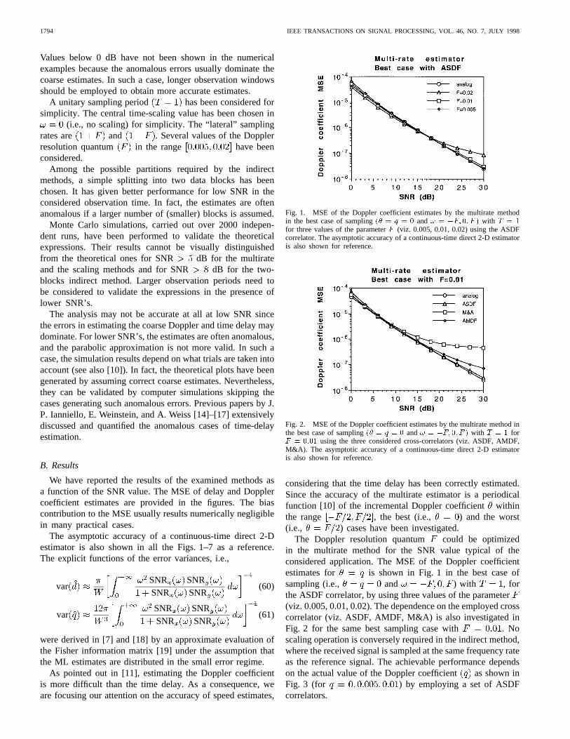
Fig. 1. MSE of the Doppler coefficient estimates by the multirate methodin the best case of sampling(� = q = 0 and! = �F; 0; F ) with T = 1for three values of the parameterF (viz. 0.005, 0.01, 0.02) using the ASDFcorrelator. The asymptotic accuracy of a continuous-time direct 2-D estimatoris also shown for reference.

Fig. 2. MSE of the Doppler coefficient estimates by the multirate method inthe best case of sampling(� = q = 0 and! = �F; 0; F ) with T = 1 forF = 0:01 using the three considered cross-correlators (viz. ASDF, AMDF,M&A). The asymptotic accuracy of a continuous-time direct 2-D estimatoris also shown for reference.

considering that the time delay has been correctly estimated.Since the accuracy of the multirate estimator is a periodicalfunction [10] of the incremental Doppler coefficientwithinthe range , the best (i.e., ) and the worst(i.e., ) cases have been investigated.

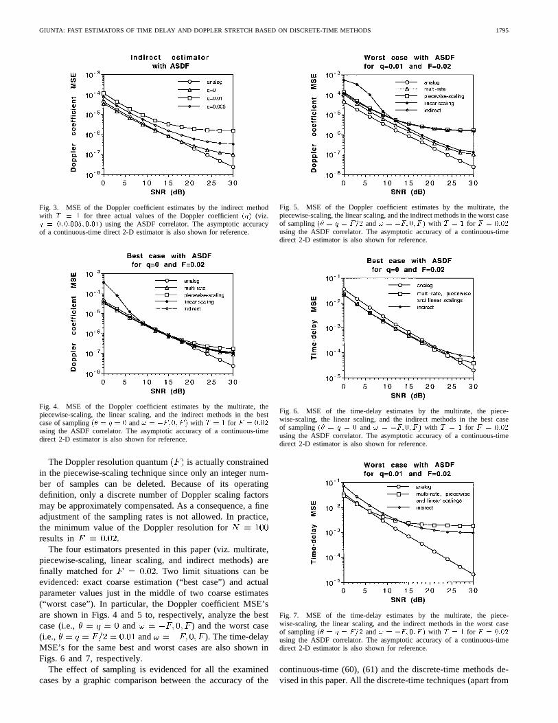
The Doppler resolution quantum could be optimizedin the multirate method for the SNR value typical of theconsidered application. The MSE of the Doppler coefficientestimates for is shown in Fig. 1 in the best case ofsampling (i.e., and ) with , forthe ASDF correlator, by using three values of the parameter(viz. 0.005, 0.01, 0.02). The dependence on the employed crosscorrelator (viz. ASDF, AMDF, M&A) is also investigated inFig. 2 for the same best sampling case with . Noscaling operation is conversely required in the indirect method,where the received signal is sampled at the same frequency rateas the reference signal. The achievable performance dependson the actual value of the Doppler coefficient as shown inFig. 3 (for ) by employing a set of ASDFcorrelators.


Fig. 3. MSE of the Doppler coefficient estimates by the indirect methodwith T = 1 for three actual values of the Doppler coefficient(q) (viz.q = 0; 0:005; 0:01) using the ASDF correlator. The asymptotic accuracyof a continuous-time direct 2-D estimator is also shown for reference.

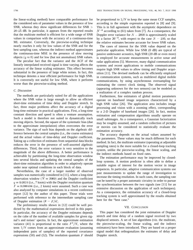
Fig. 4. MSE of the Doppler coefficient estimates by the multirate, thepiecewise-scaling, the linear scaling, and the indirect methods in the bestcase of sampling(� = q = 0 and! = �F; 0; F ) with T = 1 for F = 0:02using the ASDF correlator. The asymptotic accuracy of a continuous-timedirect 2-D estimator is also shown for reference.

The Doppler resolution quantum is actually constrainedin the piecewise-scaling technique since only an integer num-ber of samples can be deleted. Because of its operatingdefinition, only a discrete number of Doppler scaling factorsmay be approximately compensated. As a consequence, a fineadjustment of the sampling rates is not allowed. In practice,the minimum value of the Doppler resolution forresults in .

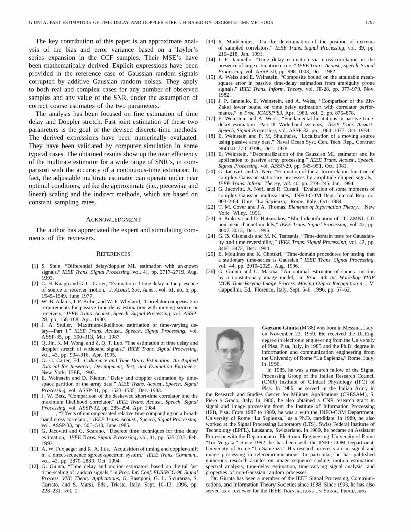
The four estimators presented in this paper (viz. multirate,piecewise-scaling, linear scaling, and indirect methods) arefinally matched for . Two limit situations can beevidenced: exact coarse estimation (“best case”) and actualparameter values just in the middle of two coarse estimates(“worst case”). In particular, the Doppler coefficient MSE’sare shown in Figs. 4 and 5 to, respectively, analyze the bestcase (i.e., and ) and the worst case(i.e., and ). The time-delayMSE’s for the same best and worst cases are also shown inFigs. 6 and 7, respectively.

The effect of sampling is evidenced for all the examinedcases by a graphic comparison between the accuracy of the

Fig. 5. MSE of the Doppler coefficient estimates by the multirate, thepiecewise-scaling, the linear scaling, and the indirect methods in the worst caseof sampling(� = q = F=2 and! = �F; 0; F ) with T = 1 for F = 0:02using the ASDF correlator. The asymptotic accuracy of a continuous-timedirect 2-D estimator is also shown for reference.

Fig. 6. MSE of the time-delay estimates by the multirate, the piece-wise-scaling, the linear scaling, and the indirect methods in the best caseof sampling(� = q = 0 and! = �F; 0; F ) with T = 1 for F = 0:02using the ASDF correlator. The asymptotic accuracy of a continuous-timedirect 2-D estimator is also shown for reference.

Fig. 7. MSE of the time-delay estimates by the multirate, the piece-wise-scaling, the linear scaling, and the indirect methods in the worst caseof sampling(� = q = F=2 and! = �F; 0; F ) with T = 1 for F = 0:02using the ASDF correlator. The asymptotic accuracy of a continuous-timedirect 2-D estimator is also shown for reference.

continuous-time (60), (61) and the discrete-time methods de-vised in this paper. All the discrete-time techniques (apart from


the linear-scaling method) have comparable performance forthe considered sets of parameter values in the presence of lowSNR, whereas they show significant differences for SNR

– dB. In particular, it appears from the reported resultsthat the multirate method is efficient for a wide range of SNRvalues in comparison with the accuracy of a continuous-timeML estimator. Conversely, the piecewise-scaling techniquenearly reaches it only for low values of the SNR and for thebest sampling case, whereas the indirect method approximatesthe continuous-time MSE in the presence of slow movingobjects and for low (but not anomalous) SNR values.

The peculiar fact that the variance and the ACF of thelinearly interpolated received signal is time varying affects theaccuracy of the linear scaling estimator. This effect becomessubstantial in the presence of large white noises. In fact, thistechnique denotes a near efficient performance for high SNR.It is conversely not useful for low SNR, where it performsworse than the piecewise-scaling method.

C. Discussion

The methods are particularly suited for all the applicationswhere the SNR value is large enough to allow an efficientshort-time estimation of time delay and Doppler stretch. Infact, three major problems affect the accuracy of a digitallong-time estimator in practical applications. First, a long-timeconstant direction and speed is often a venture assumption.Such a model is therefore not suited to dynamically trackmoving objects. Second, the square of the systematic bias (dueto the approximate interpolation) often overcomes the errorvariance. The sign of such bias depends on the algebraic dif-ference between the central samples (i.e., the coarse estimates)and the actual values of time-delay and Doppler coefficient.Taking up a collection of estimates from sequential data blocksreduces the error in the presence of well-assorted algebraicdifferences. Third, the error variance is very sensitive to themagnitude of the above difference. A better performance isachievable by partitioning the long-time observation windowinto several blocks and updating the central samples of theshort-time estimation algorithm in order to adaptively operateunder near optimal conditions in each block of data.

Nevertheless, the case of a larger number of observedsamples was numerically considered in [11], where a long-timeobservation window and the Doppler coefficient

(i.e., 7 knots) with the Doppler resolution quantum(i.e., 2 knots) were assumed. Such a case was

also analyzed by computer simulations in a recent conferencereport [12] by the author of this paper. Those trials wereperformed with reference to the intermediate sampling caseof Doppler estimation .

The preliminary results shown in [12] could be well pre-dicted by the mathematical expressions derived in this paper.In particular, the accuracy of the Doppler estimates dependson the cube of the number of available samples for given sig-nal’s and noises’ spectra. In fact, the approximate estimationvariance (41) is proportional to the ratio , where theterm comes from an approximate evaluation (assumingindependent pairs of samples) of the reported covarianceexpressions (50) and (52). The resolution quantumshould

be proportional to to keep the same mean CCF samples,according to the simple expression reported in [8] and [9].This is in full agreement with the asymptotic dependence on

according to (61) taken from [7]. As a consequence, theDoppler error variance for is approximately scaledby a factor , with respect to the case , so thatthe relative estimates become accurate for lower SNR values.

The cases of interest for the SNR value depend on theparticular application. While low SNR (0 dB) are typical ofpassive underwater acoustics, high SNR (20 dB or even more)is employed for accurate measurements in active sonar andradar applications [5]. Moreover, many digital communicationsystems and recent applications to mobile communicationsrequire high SNR values to allow timing and Doppler acqui-sition [11]. The devised methods can be efficiently employedin communication systems, such as multilevel digital mobilecommunications, by using asynchronous oversampling forestimating the correct clock timing. The observed signal(appearing unknown for the two sensors) can be modeled asa realization of a complex random process.

Furthermore, fine estimators of global motion parametersoperate on baseband image sequences characterized by ahigh SNR value [26]. The application area includes imageprocessing and vision with a zooming effect, correspondingto a 2-D Doppler of baseband images [26]. In fact, motionestimation and compensation algorithms usually operate onsmall subimages. As a consequence, a Gaussian factorizationmay be roughly assumed, and a random collection of picturesor movies can be considered to statistically evaluate theestimation accuracy.

The accuracy depends on the actual values assumed bythe parameters. These values may be much different for eachmethod. In fact, the multirate estimator (operating at adjustablesampling rates) is the more suitable for a closed-loop trackingsystem, unlike the piecewise-scaling, the linear scaling, andthe indirect methods based on fixed rates.

The estimation performance may be improved by closed-loop systems. A motion predictor is often able to define asuitable region of interest for the motion vector in imagesequences. In particular, adaptive communication systems usepast measurements to update the range of investigation toincrease the timing resolution. In such cases, the sampling ratecan be tuned by a proper automatic circuitry in order to pursuethe synchronization between the two signals (see [11] for anextensive discussion on the application of such techniques).As a consequence, the estimation accuracy of a closed-looptracking system is well approximated by the results obtainedhere for the “best case.”

VII. CONCLUSION

This paper has considered the joint estimation of Dopplerstretch and time delay of a random signal received by twodisplaced sensors. A set of fast algorithms (viz. the multirate,the piecewise-scaling, the linear scaling, and the indirectestimators) have been introduced. They are based on a propersignal model that orthogonalizes the estimates of delay andDoppler stretch.


The key contribution of this paper is an approximate anal-ysis of the bias and error variance based on a Taylor’sseries expansion in the CCF samples. Their MSE’s havebeen mathematically derived. Explicit expressions have beenprovided in the reference case of Gaussian random signalscorrupted by additive Gaussian random noises. They applyto both real and complex cases for any number of observedsamples and any value of the SNR, under the assumption ofcorrect coarse estimates of the two parameters.

The analysis has been focused on fine estimation of timedelay and Doppler stretch. Fast joint estimation of these twoparameters is the goal of the devised discrete-time methods.The derived expressions have been numerically evaluated.They have been validated by computer simulation in sometypical cases. The obtained results show up the near efficiencyof the multirate estimator for a wide range of SNR’s, in com-parison with the accuracy of a continuous-time estimator. Infact, the adjustable multirate estimator can operate under nearoptimal conditions, unlike the approximate (i.e., piecewise andlinear) scaling and the indirect methods, which are based onconstant sampling rates.

ACKNOWLEDGMENT

The author has appreciated the expert and stimulating com-ments of the reviewers.

REFERENCES

[1] S. Stein, “Differential delay/doppler ML estimation with unknownsignals,” IEEE Trans. Signal Processing, vol. 41, pp. 2717–2719, Aug.1993.

[2] C. H. Knapp and G. C. Carter, “Estimation of time delay in the presenceof source or receiver motion,”J. Acoust. Soc. Amer., vol. 61, no. 6, pp.1545–1549, June 1977.

[3] W. B. Adams, J. P. Kuhn, and W. P. Whyland, “Correlator compensationrequirements for passive time-delay estimation with moving source orreceivers,”IEEE Trans. Acoust., Speech, Signal Processing, vol. ASSP-28, pp. 158–168, Apr. 1980.

[4] J. A. Stuller, “Maximum-likelihood estimation of time-varying de-lay—Part I,” IEEE Trans. Acoust., Speech, Signal Processing, vol.ASSP-35, pp. 300–313, Mar. 1987.

[5] Q. Jin, K. M. Wong, and Z. Q. T. Luo, “The estimation of time delay anddoppler stretch of wideband signals,”IEEE Trans. Signal Processing,vol. 43, pp. 904–916, Apr. 1995.

[6] G. C. Carter, Ed.,Coherence and Time Delay Estimation. An AppliedTutorial for Research, Development, Test, and Evaluation Engineers,New York: IEEE, 1993.

[7] E. Weinstein and D. Kletter, “Delay and doppler estimation by time-space partition of the array data,”IEEE Trans. Acoust., Speech, SignalProcessing, vol. ASSP-31, pp. 1523–1535, Dec. 1983.

[8] J. W. Betz, “Comparison of the deskewed short-time correlator and themaximum likelihood correlator,”IEEE Trans. Acoust., Speech, SignalProcessing, vol. ASSP-32, pp. 285–294, Apr. 1984.

[9] , “Effects of uncompensated relative time companding on a broad-band cross correlator,”IEEE Trans. Acoust., Speech, Signal Processing,vol. ASSP-33, pp. 505–510, June 1985.

[10] G. Jacovitti and G. Scarano, “Discrete time techniques for time delayestimation,”IEEE Trans. Signal Processing, vol. 41, pp. 525–533, Feb.1993.

[11] A. W. Fuxjaeger and R. A. Iltis, “Acquisition of timing and doppler-shiftin a direct-sequence spread-spectrum system,”IEEE Trans. Commun.,vol. 42, pp. 2870–2880, Oct. 1994.

[12] G. Giunta, “Time delay and motion estimators based on digital fasttime-scaling of random signals,” inProc. Int. Conf. EUSIPCO-96 SignalProcess. VIII; Theory Applications, G. Ramponi, G. L. Sicuranza, S.Carrato, and S. Marsi, Eds., Trieste, Italy, Sept. 10–13, 1996, pp.228–231, vol. 1.

[13] R. Moddemijer, “On the determination of the position of extremaof sampled correlators,”IEEE Trans. Signal Processing, vol. 39, pp.216–218, Jan. 1991.

[14] J. P. Ianniello, “Time delay estimation via cross-correlation in thepresence of large estimation errors,”IEEE Trans. Acoust., Speech, SignalProcessing, vol. ASSP-30, pp. 998–1003, Dec. 1982.

[15] A. Weiss and E. Weinstein, “Composite bound on the attainable mean-square error in passive time-delay estimation from ambiguity pronesignals,” IEEE Trans. Inform. Theory, vol. IT-28, pp. 977–979, Nov.1982.

[16] J. P. Ianniello, E. Weinstein, and A. Weiss, “Comparison of the Ziv-Zakai lower bound on time delay estimation with correlator perfor-mance,” inProc. ICASSP’83, Apr. 1983, vol. 2, pp. 875–878.

[17] E. Weinstein and A. Weiss, “Fundamental limitations in passive time-delay estimation—Part II: Wide-band systems,”IEEE Trans. Acoust.,Speech, Signal Processing, vol. ASSP-32, pp. 1064–1077, Oct. 1984.

[18] E. Weinstein and P. M. Shultheiss, “Localization of a moving sourceusing passive array data,” Naval Ocean Syst. Cen. Tech. Rep., ContractN66001-77-C-0396, Dec. 1978.

[19] E. Weinstein, “Decentralization of the Gaussian ML estimator and itsapplication to passive array processing,”IEEE Trans. Acoust., Speech,Signal Processing, vol. ASSP-29, pp. 945–951, Oct. 1981.

[20] G. Jacovitti and A. Neri, “Estimation of the autocorrelation function ofcomplex Gaussian stationary processes by amplitude clipped signals,”IEEE Trans. Inform. Theory, vol. 40, pp. 239–245, Jan. 1994.

[21] G. Jacovitti, A. Neri, and R. Cusani, “Evaluation of some moments ofcomplex Gaussian multivariates,” INFO-COM Dept. Internal Rep. no.003-2-84, Univ. “La Sapienza,” Rome, Italy, Oct. 1984.

[22] T. M. Cover and J.A. Thomas,Elements of Information Theory. NewYork: Wiley, 1991.

[23] S. Prakriya and D. Hatzinakos, “Blind identification of LTI-ZMNL-LTInonlinear channel models,”IEEE Trans. Signal Processing, vol. 43, pp.3007–3013, Dec. 1995.

[24] G. B. Giannakis and M. K. Tsatsanis, “Time-domain tests for Gaussian-ity and time-reversibility,”IEEE Trans. Signal Processing, vol. 42, pp.3460–3472, Dec. 1994.

[25] E. Moulines and K. Choukri, “Time-domain procedures for testing thata stationary time-series is Gaussian,”IEEE Trans. Signal Processing,vol. 44, pp. 2010–2025, Aug. 1996.

[26] G. Giunta and U. Mascia, “An optimal estimator of camera motionby a nonstationary image model,” inProc. 4th Int. Workshop TVIPMOR Time-Varying Image Process. Moving Object Recognition 4,, V.Cappellini, Ed., Florence, Italy, Sept. 5–6, 1996, pp. 57–62.

Gaetano Giunta(M’88) was born in Messina, Italy,on November 23, 1959. He received the Dr.Eng.degree in electronic engineering from the Universityof Pisa, Pisa, Italy, in 1985 and the Ph.D. degree ininformation and communication engineering fromthe University of Rome “La Sapienza,” Rome, Italy,in 1990.

In 1985, he was a research fellow of the SignalProcessing Group of the Italian Research Council(CNR) Institute of Clinical Physiology (IFC) ofPisa. In 1986, he served in the Italian Army in

the Research and Studies Center for Military Applications (CRESAM), S.Piero a Grado, Italy. In 1986, he also obtained a CNR research grant insignal and image processing from the Institute of Information Processing(IEI), Pisa. From 1987 to 1989, he was a with the INFO-COM Department,University of Rome “La Sapienza,” as a Ph.D. candidate. In 1989, he alsoworked at the Signal Processing Laboratory (LTS), Swiss Federal Institute ofTechnology (EPFL), Lausanne, Switzerland. In 1989, he became an AssistantProfessor with the Department of Electronic Engineering, University of Rome“Tor Vergata.” Since 1992, he has been with the INFO-COM Department,University of Rome “La Sapienza.” His research interests are in signal andimage processing in telecommunications. In particular, he has publishednumerous research articles on image sequence coding, motion estimation,spectral analysis, time-delay estimation, time-varying signal analysis, andproperties of non-Gaussian random processes.

Dr. Giunta has been a member of the IEEE Signal Processing, Communi-cations, and Information Theory Societies since 1988. Since 1993, he has alsoserved as a reviewer for the IEEE TRANSACTIONS ON SIGNAL PROCESSING.

Fast estimators of time delay and Doppler stretch based on discrete-time methods

Documents