Fast error analysis of continuous GPS observations

J Geod (2008) 82:157–166DOI 10.1007/s00190-007-0165-x

ORIGINAL ARTICLE

Fast error analysis of continuous GPS observations

M. S. Bos · R. M. S. Fernandes ·S. D. P. Williams · L. Bastos

Received: 8 September 2006 / Accepted: 7 May 2007 / Published online: 18 July 2007© Springer-Verlag 2007

Abstract It has been generally accepted that the noisein continuous GPS observations can be well described bya power-law plus white noise model. Using maximum like-lihood estimation (MLE) the numerical values of the noisemodel can be estimated. Current methods require calculatingthe data covariance matrix and inverting it, which is a signifi-cant computational burden. Analysing 10 years of daily GPSsolutions of a single station can take around 2 h on a regu-lar computer such as a PC with an AMD Athlon™ 64 X2dual core processor. When one analyses large networks withhundreds of stations or when one analyses hourly insteadof daily solutions, the long computation times becomes aproblem. In case the signal only contains power-law noise,the MLE computations can be simplified to a O(N log N )

Electronic supplementary material The online version of thisarticle (doi:10.1007/s00190-007-0165-x) contains supplementarymaterial, which is available to authorized users.

M. S. Bos (B) · L. BastosUniversity of Porto, Monte da Virgem,4430-146 Vila Nova de Gaia, Portugale-mail: [email protected]

L. Bastose-mail: [email protected]

R. M. S. FernandesUniversity of Beira Interior, CGUL, IDL,R. Marquês d’Ávila e Boloma, 6201-001 Covilhã, Portugal

R. M. S. FernandesDelft University of Technology, DEOS,Kluyverweg 1, 2629 HS Delft, The Netherlandse-mail: [email protected]

S. D. P. WilliamsProudman Oceanographic Laboratory,6 Brownlow Street, Liverpool L3 5DA, UKe-mail: [email protected]

process where N is the number of observations. For thegeneral case of power-law plus white noise, we present amodification of the MLE equations that allows us to reducethe number of computations within the algorithm from acubic to a quadratic function of the number of observationswhen there are no data gaps. For time-series of three and eightyears, this means in practise a reduction factor of around 35and 84 in computation time without loss of accuracy. In addi-tion, this modification removes the implicit assumption thatthere is no environment noise before the first observation.Finally, we present an analytical expression for the uncer-tainty of the estimated trend if the data only contains power-law noise.

Keywords GPS · Power-law · Correlated noise ·Time-series analysis

1 Introduction

Error analysis of the estimates of continuous GPS positionshave received a lot of attention in the last few years (Zhanget al. 1997; Mao et al. 1999; Williams et al. 2004). It is nowestablished that GPS residuals show temporal correlation andthat this has to be taken into account to produce realistic errorbars on the GPS-derived velocities. This temporal correla-tion in the noise is usually described by a power-law pluswhite noise model. The latter has equal power at all frequen-cies, while the power-law is defined by its power spectrumP (Agnew 1992; Kasdin 1995):

P( f ) = P0

f α(1)

where f is the frequency, P0 a constant and α the spectralindex.

123

158 M. S. Bos et al.

The problem is then reduced to estimating the spectralindex of the power-law and the estimation of the amplitudesof the power-law and white noise random variables. Mao et al.(1999) showed that the most accurate results are obtainedwith maximum likelihood estimation (MLE). However, thecurrent formulation of the MLE for GPS time-series data iscomputationally intensive and grows with the cube of thenumber of observations.

This paper presents a simple modification of the MLEequations, which enables us to reduce the required numberof operations to a quadratic function when there are no datagaps. At the same time, the new algorithm avoids the stan-dard implicit assumption that there is no noise before the firstobservation has been made.

2 Review of current GPS error analysis techniques

If each data point xi is independent, normally distributed andif it has a standard deviation of σi , then the following equa-tion follows a χ2 probability distribution with N −M degreesof freedom:

χ2 =N∑

i=1

(xi − x̂i

σi

)2

(2)

where N is the number of observations and M is the numberof parameters used to estimate x̂.

Since Eq. (2) involves taking the difference between theobservations and the estimated model, it produces an indica-tion of the goodness of fit. For a large number of data points,say 30, the value χ2 is approximately N − M . The reducedchi-square is defined as χ2/(N − M) and consequently has avalue around one. When the reduced χ2 value is much largerthan one, it indicates that the estimated model is wrong orthat the assumed errors are too small.

GPS analysis software provides standard deviations foreach estimated station position, but in almost all cases theseare too small to be realistic. To get better error values, theyare usually scaled by

√χ2/(N − M). This empirical reduced

chi-square method is widely used within the geodetic com-munity, but is not the correct solution to improve the errorbars. The problem is that one assumes that the GPS residualsare independent from each other, while in reality they show astrong correlation in time (Johnson and Agnew 1995). Maoet al. (1999) have shown that after applying the reduced χ2

value, the real error can still be underestimated by a factor of5–11.

Figure 1 shows the North component of the GPS time-series at Kootwijk (KOSG), The Netherlands. It also showsthe residuals after subtracting the least-squares estimated lin-ear motion. From these residuals, the power-spectrum wascomputed and is shown in Fig. 2. It illustrates the need for an

-6

-4

-2

0

2

4

1996 1998 2000 2002 2004 2006

Res

idua

l (m

m)

Time (years)

0

40

80

120

160

Nor

th (

mm

)

Fig. 1 The upper panel shows the North component of the GPS posi-tion time-series at KOSG. The lower panel shows the same data setafter subtraction of a linear trend, a yearly signal and one offset

105

106

107

10-8 10-7 10-6 10-5

Pow

er (

mm

2 /Hz)

Frequency (Hz)

Fig. 2 Power spectrum of the GPS residuals at KOSG, North compo-nent. The circles denote the spectrum computed from the observationsand the solid line is the fitted power-law plus white noise model

improved noise model. In the high frequencies, the noise isflat (property of white noise), while for the lower frequencies,the spectrum seems to obey a power-law. The slope of thepower-law is around one, which is sometimes called flickernoise. Williams et al. (2004) have shown that the power spec-tra in Fig. 2 is representative for many GPS residuals.

Following Langbein and Johnson (1997) and Kasdin(1995), the spectral index is represented by α. A power-lawnoise time-series, say r, with a spectral index between −1and 1 can be generated by convolving it with independentand identically distributed (IID) noise wk (Hosking 1981):

rk =∞∑

i=0

hi wk−i (3)

123

Fast error analysis of continuous GPS observations 159

where, following Kasdin (1995)

h0 = 1

hi =(α

2+ i − 1

) hi−1

i

(4)

These relations follow from Hosking’s definition of thefractional difference operation:

(1 − B)α/2 =∞∑

i=0

(α/2

i

)(−B)i

=∞∑

i=0

Γ (α/2 + 1)

Γ (α/2 − i + 1) i ! (−B)i

= 1 − α

2B − 1

2

α

2

(1 − α

2

)B2 − · · · (5)

where Γ is the Gamma function and B is the backward-shiftoperator (Bxk = xk−1). From this definition, one can deducethat:

(1 − B)α/2rk = wk (6a)

(1 − B)−α/2wk = rk (6b)

In order to apply the backward-shift operator, Eq. (6a)assumes the existence of an infinite amount of r before rk ,while Eq. (6b) assumes the same for w.

In this research, since we observe a finite amount of signalwith coloured noise r, we will concern ourselves mostly withEq. (6b). The covariance between rk and rl only depends onτ = l − k. It thus forms a Toeplitz matrix, which can bewritten as Cov(rk, rl) = γ (τ). A Toeplitz matrix is a matrixin which each descending diagonal from left to right is con-stant. If one assumes an infinite sequence of zero-mean whitenoise w, with variance σ 2

pl , then the covariance is (Hosking1981; Appendix A):

γ (0) = σ 2pl

Γ (1 − α)

(Γ (1 − α2 ))2

γ (τ) =α2 + τ − 1

−α2 + τ

γ (τ − 1) for τ > 0 (7)

The covariance of Eq. (7) only exists for α < 1. For α ≥ 1,the noise is not stationary and therefore produces an infi-nite variance. Since the power-law noise in GPS may have aspectral index larger than one, this causes a problem. For thisreason, one usually assumes that wi = 0 for i < 0, whichmeans that the sum only runs to k to produce finite covari-ance values. With this assumption, the covariance betweenrk and rl with l > k is:

Cov(rk, rl) = σ 2pl

k∑

i=0

hi hi+(l−k) (8)

Equation (8) can also be written as a matrix multiplicationC = UT U. Matrix U is an upper triangular matrix and looks

like:

U =

⎛

⎜⎜⎜⎝

h0 h1 . . . hN

0 h0 hN−1...

. . ....

0 0 . . . h0

⎞

⎟⎟⎟⎠ (9)

Using Eq. (3) and again assuming that wi = ri = 0 for i < 0,one has the following relations:

r = UT w (10a)

w = U−T r (10b)

For clarity, we have omitted the scaling factor ∆T α/2 used byWilliams (2003), where ∆T is the sampling interval, sincewe will only discuss daily GPS solutions here.

To get the total noise, pure white noise with variance σ 2w

has to be added to the power-law noise. Writing Eq. (8) as amatrix E(α) and using I for the unit matrix, the new covari-ance matrix C for the GPS data can be written as (Langbeinand Johnson, 1997; Langbein, 2004; Williams, 2003):

C = σ 2wI + σ 2

plE(α) (11)

The east, north and up components all have a separatecovariance matrix C. The GPS solutions provide a spatial cor-relation between the components but this is normallyneglected when Eq. (11) is considered because they are smallcompared to the temporal correlations. Furthermore, it isassumed that, for each component, the variances are equalat each data point. This condition is mostly met in practise.

2.1 Maximum likelihood estimation

To estimate the parameters that describe the trend in the GPSobservations and the parameters of the noise model, we mustmaximise the probability p that their values have occurred forgiven observations x. If a Gaussian distribution is assumed,then this probability is:

p(x) = 1

(2π)N2 det

12 (C)

× exp

[−1

2(x − Hθ̂ot )

T C−1(x − Hθ̂ot )

](12)

where the vector θ̂ot contains the parameters for the nomi-nal value, which is the offset of the whole time-series andthe trend. The observation matrix H has N rows and 2 col-umns. The first contains solely ones, while the second col-umn contains a linear trend. Langbein (2004) notes that itis straightforward to include also a yearly signal and offsetsin the estimation process. Note that the observed minus theestimated trend will produce the residuals r discussed in theSect. 2: r = x − Hθ̂ot .

123

160 M. S. Bos et al.

In practise, the maximum of the logarithm of this probabil-ity p is computed, which is an equivalent problem becausethe logarithm is a monotonically increasing function. Thecovariance matrix C depends on the noise and not on θ̂ot .Therefore, the maximum can be found by setting the deriva-tive of the logarithm of Eq. (12) to zero.

After some rearrangement, one finds:

θ̂ot =(

HT C−1H)−1

HT C−1x (13)

This is the formula for weighted least squares. Using Eq. (13),the values for the noise parameters α, σpl and σw must befound by numerically maximising:

ln(p(x)) = −1

2

[N ln(2π) + ln det(C)

+ (x − Hθ̂ot )T

C−1(x − Hθ̂ot )

](14)

Details about this computation are given by Langbein andJohnson (1997) and Langbein (2004).

3 Remaining problems

MLE provides a reliable error estimate for the trend (Maoet al. 1999). However, its main disadvantage is the compu-tation time. Analysing the North, East and Up componentof 10 years of daily GPS solutions of one station can take aslong as two hours on a regular computer such as a PC withan AMD Athlon™ 64 X2 Dual Core Processor. The erroranalysis of large networks or the analysis of hourly solutionscan therefore take several days.

The causes of the relatively long computation time are theconstruction of the covariance matrix and the computation ofEqs. (13) and (14), all requiring O(N 3) operations. For thisreason, the spectral index is often a priori fixed to a value ofone to accelerate the process.

Another approach is to estimate the noise propertiesdirectly from the power-spectrum (Mao et al. 1999), which isextremely fast because the power-spectrum can be computedwith only O(N log N ) operations for evenly spaced data.However, we prefer the MLE method because it allows con-sistent estimates of the components of the covariance func-tion and the parameters of the time-dependent model of thedata (Langbein 2004).

4 Fast power-law noise analysis

If the noise consists only of pure power-law noise, then thelogarithm of the determinant of the covariance matrix is, forall α, equal to 2N ln σpl . To compute the likelihood func-tion (Eq. 14), it would be desirable to have a fast way to

compute C−1. Hosking (1981) describes how the movingaverage equation for the noise can be rewritten as an autore-gressive representation:

wk =∞∑

i=0

pirk−i (15)

where

p0 = 1

pi =(−α

2+ i − 1

) pi−1

i

(16)

The advantage of this formulation is that it allows us tocompute the inverse of the covariance matrix C directly.Remember that we had assumed that wi = ri = 0 fori < 0, which has the consequence that the summation ofEq. (15) must be truncated to k. Furthermore, using the rela-tion C−1 = U−1U−T and Eq. (10b), we get with pi = 0 fori < 0:

(Cov(rk, rl))−1 =

N−k∑

i=0

pi pi+(k−l) (17)

In the likelihood function (Eq. 14), we need to computerT C−1r. If one writes the elements pi in a lower triangu-lar matrix L = U−T , this becomes: (Lr)T (Lr). A majorreduction in computation time is achieved by taking advan-tage of the fact that Lr is a convolution operation with filterpi , which ‘whitens’ the residuals r. In Eq. (13) the samefilter operation is applied to each column of H. Press et al.(1988) describe how this can be efficiently computed withfast Fourier transform in O(N log N ) operations. Thus theMLE for pure power-law noise can be reduced from O(N 3)

to O(N log N ) operations for this special case.Before ending this section, we will present the inverse of

the covariance matrix C when the number of observationsgoes to infinity. This inverse is well behaved for α > −1 andconverges to the following Toeplitz matrix, Cov−1(rk, rl) =γ −1(τ ), with τ = l − k:

γ −1(0) = 1

σ 2pl

Γ (1 + α)(Γ (1 + α

2 ))2

γ −1(τ ) = τ − 1 − α2

τ + α2

γ −1(τ − 1) for τ > 0 (18)

Using Eqs. (6a) and (6b), one can see that this is the resultof changing α/2 with −α/2 in Eq. (7). Equation (18) onlyrepresents the approximation of the inverse of the covariancematrix when the number of observations grows to infinity.Thus, in practise one still has to use Eq. (17) where the sum-mations are taken up to N − k since wk , and therefore rk , arezero for k < 0.

If there really is no noise before the first observation ismade, it would be better to stop and restart the observationsas often as possible to avoid any power-law noise to develop

123

Fast error analysis of continuous GPS observations 161

in the time-series. Intuitively this is incorrect since the startof the observations has no physical effect on the GPS monu-mentation, which Langbein and Johnson (1997) consider tobe the cause of some of the power-law noise. This problemis solved in the next section.

5 A fast alternative

In Sect. 2, it was stated that power-law noise can be gener-ated by convolving white noise with a transfer function h.Since we do not know anything about the signal before thefirst observation, the convolution in Eq. (3) was taken onlyover all the available data points. However, now we make theassumption that the noise is present prior to the start of theobservations and that the convolution summation needs betaken to infinity.

Unfortunately, for α ≥ 1, the noise is non-stationary andthe summation would grow to infinity. For this reason, Agnew(1992) used a structure function that is defined as the differ-ence between two observations at time t and time t + T .Here, only the discrete case will be discussed and the differ-ence of the GPS residuals will be restricted to one time step,∆rk = rk+1−rk . Using Eq. (3), this can be written as (Kasdin1995)

∆rk = wk+1 +(α

2− 1

) k∑

i=0

hi

i + 1wk−i (19)

The same difference can be taken between the points rl+1

and rl . The power-law covariance between these two firstdifferences is, with τ = k − l, k ≥ l:

Cov (∆rk,∆rl)

= σ 2pl

[1 +

(α

2− 1

)2 l∑

i=0

h2i

(i + 1)2

]for k = l

= σ 2pl

[(α

2− 1

) hτ−1

τ+

(α

2− 1

)2

×l∑

i=0

hi+τ hi

(i + τ + 1)(i + 1)

]for k �= l (20)

Equation (20) is the exact equivalent to the covariance matrixof Eq. (8), but for first-differenced data.

Let us now apply our assumption that the first observationis already affected by noise and that this noise, because wetook the first difference, is stationary. In this case, we canextend our summations in Eq. (20) to infinity. Using Eq. (4)and some hypergeometric function relations (Abramowitzand Stegun 1965) the covariance Cov(∆rk,∆rl) = Cov(∆rl ,

∆rk) = γpl(τ ) can be written as, see Appendix A:

γpl(0) = σ 2pl

Γ (3 − α)

(Γ (2 − α2 ))2

γpl(τ ) =α2 + τ − 2

1 − α2 + τ

γpl(τ − 1) for τ > 0 (21)

Equation (21) is the same as Eq. (7) but with α/2 replacedby α/2−1, which causes it to be valid for α < 3. The advan-tage of the covariance matrix given by Eq. (21) is that its con-struction takes O(N ) instead of O(N 3) operations becauseonly the vector γpl needs to be known to describe the wholematrix. Looking back at Eq. (6a), one can see that Eq. (21) isthe result of rewriting the definition of the fractional differ-ence:

(1 − B)α/2r = (1 − B)α/2−1 (1 − B)r

= (1 − B)α/2−1∆r (22)

The covariance between two first differenced white noiseobservations is:

γw(0) = 2σ 2w

γw(1) = −σ 2w

γw(τ) = 0 for τ > 1. (23)

The sum of power-law and white noise still produces aToeplitz matrix. Using the algorithm of Bojanczyk et al.(1995), the Cholesky decomposition of the Toeplitz covari-ance matrix can be performed in O(N 2) operations. Let uswrite this decomposition as C = UT U, where U is an uppertriangular matrix. A further reduction in computation timecan be obtained by rewriting Eq. (13) as

θ̂ot =(

HT (UT U)−1H)−1

HT (UT U)−1x

=(

AT A)−1

AT y (24)

where

UT A = H (25a)

UT y = x (25b)

Equations (25a) and (25b) can be directly solved by back-substitution because U is an upper triangular matrix. Alsonote that H and x now represent the first-differenced designmatrix and the first-differenced observations.

Finally, one can compute the determinant and matricesA and y while performing the Cholesky factorisation. Thefactorisation computes each column i of matrix U with onlythe information of the column i − 1, except for the first col-umn which is computed directly using γ [Eq. (21) plus Eq.(23)]. Thus only two columns of U need to be stored duringthe Cholesky decomposition, which is again beneficial forreducing the computation time. The full algorithm is givenin Appendix B.

123

162 M. S. Bos et al.

It must be noted that the first-differenced design matrix Hno longer contains the nominal value of the whole time-seriesbecause we took the difference of the observations. Since thiswas a nuisance parameter, this is only to our advantage. Fur-thermore, the observation matrix can easily be extended toinclude other signals such as, for example, a yearly signal.

6 Analytical expressions for the slope uncertainty

The variance of the estimated slope can be computed with:

σ 2r̂ =

(HT C−1H

)−1(26)

Let us assume that the data only contains power-law noise.The design matrix H consists for first-differenced data onlyout of one column with ones. Using Eq. (21), one can nowderive the following recurrence relations for the slope uncer-tainty σr̂ , for a time-series with N observations:

σ 2r̂ (2) = σ 2

pl

∆T 2− α2

Γ (3 − α)

Γ (2 − α2 )2

σ 2r̂ (N ) = N − 2

N + 1 − ασ 2

r̂ (N − 1) for N > 2 (27)

Note that we have introduced here the scaling factor ∆T ,the sampling period, to facilitate the comparison with earlierresults. The explicit form of Eq. (27) is:

σ 2r̂ = σ 2

pl

∆T 2− α2

Γ (3 − α)Γ (N − 1)Γ (4 − α)

(Γ (2 − α2 ))2Γ (N + 2 − α)

(28)

For large values of N , the Gamma function is difficult tocompute. A good approximation, however, can be obtainedwith the use of Stirling’s formula (Abramowitz and Stegun1965). Using this approximation, we get the following equa-tion for the variance of the estimated slope:

σ 2r̂ ≈ σ 2

pl

∆T 2− α2

Γ (3 − α)Γ (4 − α)(N − 1)α−3

(Γ (2 − α2 ))2 (29)

By setting α = 0, one can verify that Eq. (28) produces thesame expression for white noise as calculated by Zhang et al.(1997) among others:

σ 2r̂ = 12σ 2

pl

∆T 2(N 3 − N )(30)

and the same expression for random walk noise (α = 2):

σ 2r̂ = σ 2

pl

∆T (N − 1)(31)

Thus, for these two special cases, there is no effect whentaking into account the noise before the first observation. Thiscan be explained by the fact that white noise does not dependon past values, while the random walk noise before t = 0 willonly cause a change in the nominal value. However, for all

0.60

0.80

1.00

1.20

1.40

1.60

100 101 102 103 104 105

frac

tion

Length of time-series (days)

Eq. (32)Williams, 2003

Eq. (29), Stirling

Fig. 3 Trend uncertainties computed using different formulas, dividedby our reference trend uncertainty as defined in the text. All for flickernoise (α = 1)

other values of the spectral index, there is a slight difference.A new result is that we now have an analytical expression forthe case of flicker noise (α = 1):

σ 2r̂ = 8σ 2

pl

π∆T32 (N 2 − N )

(32)

Equations (29) and (32) are new results, and it is interest-ing to compare them with the standard trend uncertainty thatis computed, without taking first-differences, by construct-ing the covariance matrix using Eq. (8) and inserting it intoEq. (26). As was mentioned before, flicker noise is the mostcommon type of power-law noise observed in GPS data, thusα will be set to one. This standard trend uncertainty will beour reference to which the new equations will be compared.

Williams (2003) provided an approximation for the ref-erence trend uncertainty, which will also be included in thecomparison. Figure 3 shows the standard deviation of the esti-mated slope using Eq. (32), the Stirling approximation Eq.(29) and the approximation of Williams (2003) as function ofthe length of the time-series. These three trend uncertaintieshave been divided by our reference trend uncertainty to makeit easier to see their differences.

Figure 3 shows that after 100 days, the Williams approx-imation is in very good agreement with our reference trenduncertainty because the fraction goes to unity. After 100 days,the Stirling approximation, Eq. (29), is in good agreementwith Eq. (32). Figure 3 also shows that the new method gives,for time-series longer than 1,000 days, a value for the trenduncertainty that is around 15–20% larger than the referencetrend uncertainty. One could argue that the reference trenduncertainty is in fact 15–20% too small and that the newmethod, with its associated uncertainty, is in fact more real-istic because the original method does not account for noisebefore the start of the series.

Figure 4 shows the error in the estimated trend as functionof the data span using the noise properties that are observed

123

Fast error analysis of continuous GPS observations 163

10-3

10-2

102 103

tren

d er

ror

(mm

/yea

r)

Length of time-series (days)

first-differenced (white + power-law)normal (white + power-law)

Eq. (29) (only power-law)

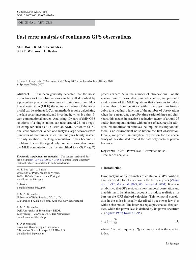
Fig. 4 The trend uncertainty at KOSG for the North component asfunction of the observation span, using the white plus power-law noiseproperties observed in these data. The solid line is computed using un-differenced data, the dashed line for first-differenced data. The pointshave been computed under the assumption that only power-law noise ispresent

in the North component of the GPS time-series at KOSG.In Fig. 4, the uncertainty was computed using Eq. (26) withthe normal covariance matrix of Eq. (11) and the first-differ-enced covariance matrix, which is the sum of Eqs. (21) and(23). The trend uncertainty was also computed using onlypower-law noise (Eq. 29).

As was observed in Fig. 3, Fig. 4 shows that the newcovariance matrix for first-differenced data produces a largertrend uncertainty than the reference trend uncertainty. Fig-ure 4 also shows that, after 2 years, the trend uncertaintiesfor first-differenced data of the power-law noise only and thepower-law plus white noise are equal. Thus after 2 years, thepower-law noise completely dominates the uncertainty, andthe contribution of the white noise can be neglected.

Mao et al. (1999) concluded that the velocity error intime-series could be underestimated by factors of 5–11 ifa pure white noise model is assumed. Taking into accountthat Eq. (32) produces larger values than the reference trenduncertainty used by Mao et al. (1999), these factors can growup to 6–13.

7 Numerical results

Section 6 presented analytical expressions for the trend uncer-tainty for given noise parameters of the power-law noise. Inreality, we are confronted with power-law plus white noisein the GPS data of which the parameter values are unknown.To test the performance of the normal MLE and the newfirst-differenced MLE approach, one hundred synthetic time-series with 1,000 and 3,000 days were generated, which havethe same trend values and noise properties as observed in theNorth component of KOSG data.

The mean values of the estimated parameters and theirobserved standard deviation using the two MLE approaches

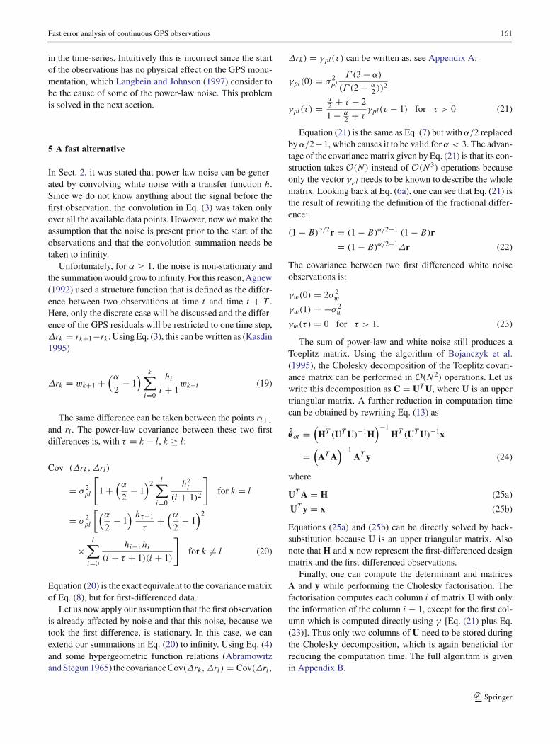
are given in Table 1. These values were obtained by imple-menting the algorithms described in Sects. 2 and 5 and usingthe BLAS and LAPACK libraries (Anderson et al. 1999),which are optimised for matrix computations.

From Table 1, one can see that for time-series of 1,000days, both MLE methods underestimate the spectral index.This was already observed by Williams et al. (2004) and isattributed to the fact that the trend will absorb some of thevery long periods of the power-law noise. For time-series of3,000 days, this bias is less.

For a very large number of synthetic time-series, theobserved standard deviation of the trend value should beequal to the predicted one for given values of the spectralindex and the variances of the power-law and white noise.Table 1 shows that, using 100 time-series of 1,000 days,both methods have an ensemble mean trend value of 15.56mm/year with a standard deviation of 0.473 and 0.489 mm/year for the normal and first-differenced MLE respectively.Using the estimated noise properties, Eqs. (11), (21), (23) and(26), the mean predicted errors are 0.398 and 0.456 mm/year,again for the normal and first-differenced MLE, respectively.

The predicted errors from the first-differenced MLE aremuch closer to the standard deviation of the trends for bothmethods, again reinforcing the notion that the new method ismore realistic. Taking the uncertainty in the predicted errorsinto account, the observed and predicted trend uncertaintiesare in good agreement. For time-series of 3,000 days, theagreement is even better.

Table 1 also lists the computation time, and shows that thenew method is indeed significantly faster. The computer usedfor these computations contained an AMD Athlon™ 64 X2Dual Core Processor 4200+, with 2 Gbyte of memory. Thecomputation times for the normal MLE and the first-differ-enced MLE methods for different lengths of the time-seriesare plotted in Fig. 5.

10-1

100

101

102

103

104

100 1000

Com

puta

tion

time

(s)

Length of time-series (days)

Normal MLEFirst-differenced MLE

Fig. 5 The computation time of the normal and first-differenced MLEmethods for different lengths of the time-series

123

164 M. S. Bos et al.

Table 1 The results of estimating the trend and noise parameters in 100time-series of 1,000 and 3,000 days where the spectral index α = 1.105,the standard deviation of the power-law noise σpl = 0.691 mm, the

standard deviation of the white noise σw = 1.393 mm and the trend is15.621 mm/year

1,000 days 3,000 days

Normal MLE Differenced MLE Normal MLE Differenced MLE

Parameter Mean σ Mean σ

α 0.917 ± 0.233 0.950 ± 0.224 1.058 ± 0.095 1.067 ± 0.093

σpl (mm) 0.858 ± 0.232 0.827 ± 0.223 0.724 ± 0.096 0.717 ± 0.093

σw (mm) 1.283 ± 0.171 1.304 ± 0.152 1.372 ± 0.051 1.375 ± 0.050

Trend (mm/year) 15.560 ± 0.473 15.564 ± 0.489 15.631 ± 0.171 15.632 ± 0.180

Predicted error (mm/year) 0.398 ± 0.155 0.456 ± 0.172 0.154 ± 0.032 0.178 ± 0.037

Mean time (s) 76 2 1348 16

The mean time indicates the average computation time of each run

8 Data gaps

So far, we have not mentioned data gaps, which are unfortu-nately present in most GPS time-series. To correct for thesegaps, one can construct, both for the normal and the first-differenced MLE method, first the full covariance matrix forthe complete time-series and afterwards delete the rows andcolumns for which no data are available (Williams 2003).

Unfortunately, the deletion of rows and columns destroysthe Toeplitz structure of the covariance matrix for the first-differenced MLE method and with that one loses the gainin computation speed. The exact solution of this problem isoutside the scope of this research, but we have experimentedwith two possible remedies.

The first one is simply filling the data gaps by linear inter-polation. We analysed 164 GPS stations with a wide rangein the length of the observation span and interpolated thedata gaps. For 90% of the stations, the trends estimated bythe normal and the first-differenced method differed by lessthan one standard deviation from each other for all threecomponents. Another approach is to ignore the gaps in thestochastic model and keep the Toeplitz covariance matrix. Inthis solution approximately 94% of the trends differed fromthe normal method by less than one standard deviation.

These results show that already with some simple meth-ods, the data gap problem can be solved in a satisfactorymanner.

9 Conclusions

It has been demonstrated that if there is only power-law noisein a continuous GPS time-series, then the normal MLE equa-tions can be computed with O(N log N ) operations. Fur-thermore, by taking the first difference of the observations,power-law noise with a spectral index value around one,

which is commonly observed in GPS observations (Williamset al. 2004), is made stationary. The new covariance matrixcan be written as a convenient recursive expression, the con-struction of which only takes O(N ) operations.

Another advantage of the new covariance matrix is that itis a Toeplitz matrix. The Cholesky factorisation of this typeof matrices can be performed in O(N 2) operations, instead ofO(N 3) for positive definite matrices. Finally, the likelihoodfunction can be computed without the explicit constructionof the covariance matrix or its Cholesky factorisation, whichagain reduces the computation time. It has been shown thatfor time-series of 1,000 and 3,000 days, a reduction factor ofaround 35 and 84 respectively in computation time can beachieved.

The modification also removed the implicit assumptionof no noise before the first observation. This generalisationmade it possible to derive an analytical expression for theuncertainty of the estimated trend in the case of pure power-law noise. Using these expressions, we conclude that thetrend uncertainty for flicker noise presented by Williams(2003) is 15–20% too small for time-series longer than threeyears and that the new method, with its associated uncer-tainty, is more realistic.

Acknowledgments We would like to thank the reviewers, JohnLangbein and Timothy Dixon, and editors for their comments that haveimproved this manuscript. M. S. Bos is supported by Fundação para aCiência e Tecnologia (FCT), through the grant SFRH/BPD/26985/2006.

Appendix A Derivation of the covariance

The coefficients hi of Eq. (4) can be written as (Kasdin 1995):

hi = (α2 )i

(1)i= Γ (α

2 + i)Γ (1)

Γ (α2 )Γ (1 + i)

= Γ (α2 + i)

Γ (α2 ) i ! (33)

123

Fast error analysis of continuous GPS observations 165

where (a)i = 1 × a × (a + 1) × · · · × (a + i − 1) denotesthe Pochammer symbol. Furthermore, the hypergeometricfunction is defined as (Abramowitz and Stegun 1965):

F(a, b; c; z) =∞∑

i=0

(a)i (b)i

(c)i

zi

i !

= Γ (c)

Γ (a)Γ (b)

∞∑

i=0

Γ (a + i)Γ (b + i)

Γ (c + i)

zi

i ! (34)

Thus, Eq. (8) can be written as:

∞∑

i=0

hi hi+τ = 1(Γ (α

2 ))2

∞∑

i=0

Γ (α2 + i)Γ (α

2 + τ + i)

Γ (1 + τ + i)

1i

i !(35)

Using the following relation (Abramowitz and Stegun 1965):

F(a, b; c; 1) = Γ (c)Γ (c − a − b)

Γ (c − a)Γ (c − b)(36)

Eq. (35) can be written as:

∞∑

i=0

hi hi+τ = Γ (α2 + τ)Γ (1 − α)

Γ (α2 )Γ (1 + τ − α

2 )Γ (1 − α2 )

(37)

Finally, with the relation Γ (τ +1) = τΓ (τ), one obtains Eq.(7). A similar derivation produces Eq. (21) from Eq. (20).

Appendix B New algorithm

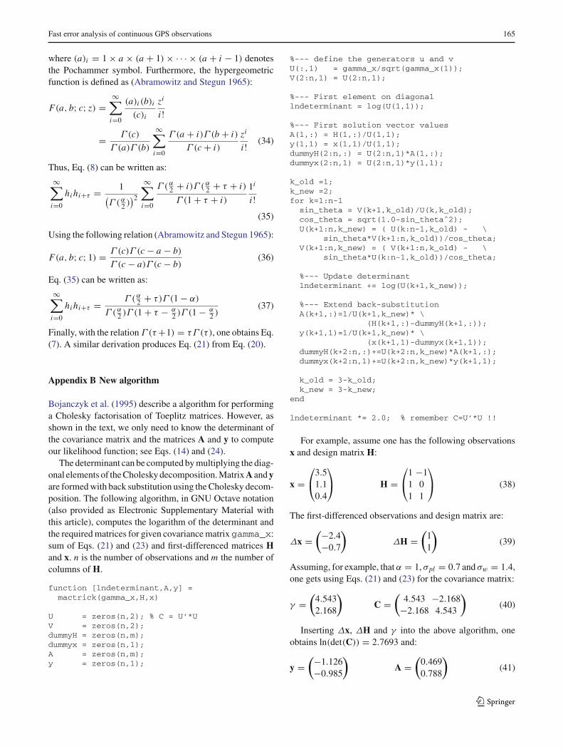
Bojanczyk et al. (1995) describe a algorithm for performinga Cholesky factorisation of Toeplitz matrices. However, asshown in the text, we only need to know the determinant ofthe covariance matrix and the matrices A and y to computeour likelihood function; see Eqs. (14) and (24).

The determinant can be computed by multiplying the diag-onal elements of the Cholesky decomposition. Matrix A and yare formed with back substitution using the Cholesky decom-position. The following algorithm, in GNU Octave notation(also provided as Electronic Supplementary Material withthis article), computes the logarithm of the determinant andthe required matrices for given covariance matrixgamma_x:sum of Eqs. (21) and (23) and first-differenced matrices Hand x. n is the number of observations and m the number ofcolumns of H.

function [lndeterminant,A,y] =mactrick(gamma_x,H,x)

U = zeros(n,2); % C = U’*UV = zeros(n,2);dummyH = zeros(n,m);dummyx = zeros(n,1);A = zeros(n,m);y = zeros(n,1);

%--- define the generators u and vU(:,1) = gamma_x/sqrt(gamma_x(1));V(2:n,1) = U(2:n,1);

%--- First element on diagonallndeterminant = log(U(1,1));

%--- First solution vector valuesA(1,:) = H(1,:)/U(1,1);y(1,1) = x(1,1)/U(1,1);dummyH(2:n,:) = U(2:n,1)*A(1,:);dummyx(2:n,1) = U(2:n,1)*y(1,1);

k_old =1;k_new =2;for k=1:n-1sin_theta = V(k+1,k_old)/U(k,k_old);cos_theta = sqrt(1.0-sin_thetaˆ2);U(k+1:n,k_new) = ( U(k:n-1,k_old) - \

sin_theta*V(k+1:n,k_old))/cos_theta;V(k+1:n,k_new) = ( V(k+1:n,k_old) - \

sin_theta*U(k:n-1,k_old))/cos_theta;

%--- Update determinantlndeterminant += log(U(k+1,k_new));

%--- Extend back-substitutionA(k+1,:)=1/U(k+1,k_new)* \

(H(k+1,:)-dummyH(k+1,:));y(k+1,1)=1/U(k+1,k_new)* \

(x(k+1,1)-dummyx(k+1,1));dummyH(k+2:n,:)+=U(k+2:n,k_new)*A(k+1,:);dummyx(k+2:n,1)+=U(k+2:n,k_new)*y(k+1,1);

k_old = 3-k_old;k_new = 3-k_new;

end

lndeterminant *= 2.0; % remember C=U’*U !!

For example, assume one has the following observationsx and design matrix H:

x =⎛

⎝3.51.10.4

⎞

⎠ H =⎛

⎝1 −11 01 1

⎞

⎠ (38)

The first-differenced observations and design matrix are:

∆x =(−2.4

−0.7

)∆H =

(11

)(39)

Assuming, for example, that α = 1, σpl = 0.7 and σw = 1.4,one gets using Eqs. (21) and (23) for the covariance matrix:

γ =(

4.5432.168

)C =

(4.543 −2.168

−2.168 4.543

)(40)

Inserting ∆x, ∆H and γ into the above algorithm, oneobtains ln(det(C)) = 2.7693 and:

y =(−1.126

−0.985

)A =

(0.4690.788

)(41)

123

166 M. S. Bos et al.

One can verify that Eq. (24) holds:(∆HT C−1∆H

)−1∆HT C−1∆x =

(AT A

)−1AT y = −1.55

(42)

References

Abramowitz M, Stegun IA (1965) Handbook of mathematical functionswith formulas, graphs and mathematical tables. National Bureau ofstandards applied mathematics series 55. US Government PrintingOffice, Washington DC

Agnew DC (1992) The time-domain behaviour of power-law noises.Geophys Res Lett 19(4):333–336

Anderson E, Bai Z, Bischof C, Blackford S, Demmel J, Dongarra J,Du Croz J, Greenbaum A, Hammarling S, McKenney A,Sorensen D (1999) LAPACK users’ guide, 3rd edn. Society forIndustrial and Applied Mathematics, Philadelphia

Bojanczyk AW, Brent RP, de Hoog FR, Sweet DR (1995) On the sta-bility of the Bareiss and related Toeplitz factorization algorithms.SIAM J Matrix Anal Appl 16(1):40–57

Hosking JRM (1981) Fractional differencing. Biometrika 68(1):165–176

Johnson HO, Agnew DC (1995) Monument motion and measurementsof crustal velocities. Geophys Res Lett 22(21):2905–2908

Kasdin NJ (1995) Discrete simulation of colored noise and stochas-tic processes and 1/ f α power law noise generation. Proc IEEE83(5):802–827

Langbein J (2004) Noise in two-color electronic distance meter mea-surements revisited. J Geophys Res 109, B04406, doi:10.1029/2003JB002819

Langbein J, Johnson H (1997) Correlated errors in geodetic timeseries: Implications for time-dependent deformation. J GeophysRes 102(B1):591–603

Mao A, Harrison CGA, Dixon TH (1999) Noise in GPS coordinate timeseries. J Geophys Res 104(B2):2797–2816

Press WH, Flannery BP, Teukolsky SA, Vetterling WT (1988) Numer-ical recipes in C. 2nd edn. University Press, Cambridge

Williams SDP (2003) The effect of coloured noise on the uncertain-ties of rates from geodetic time series. J Geod 76(9–10):483–494,doi:10.1007/s00190-002-0283-4

Williams SDP, Bock Y, Fang P, Jamason P, Nikolaidis RM,Prawirodirdjo L, Miller M, Johnson DJ (2004) Error analysis ofcontinuous GPS position time series. J Geophys Res 109, B03412,doi:10.1029/2003JB002741

Zhang J, Bock Y, Johnson H, Fang P, Williams S, Genrich J, Wdowin-ski S, Behr J (1997) Southern California permanent GPS geodeticarray: error analysis of daily position estimates and site velocities.J Geophys Res 102(B8):18035–18055

123