FAST CONTINUOUS SWIMMING OF TWO PELAGIC …jeb.biologists.org/content/jexbio/109/1/209.full.pdfFAST CONTINUOUS SWIMMING OF TWO PELAGIC PREDATORS, SAITHE ... Both species are o f course

J. exp. Biol. 109, 209-228 (1984) 2 0 9Printed in Great Britain © The Company of Biologists Limited 1984

FAST CONTINUOUS SWIMMING OF TWO PELAGICPREDATORS, SAITHE (POLLACHIUS VIRENS) AND

MACKEREL (SCOMBER SCOMBRUS): A KINEMATICANALYSIS

BY J. J. VIDELER AND F. HESS

Department of Zoology, State University Groningen, P.O. Box 14, 9750AA Haren, The Netherlands

Accepted 7 October 1983

SUMMARY

Straight, forward, unrestrained swimming behaviour, with periodiclateral oscillations of body and tailfin, was described and compared for saitheand mackerel. A method was developed for kinematic analysis of forwardmotion, lateral displacements and body curvature, based on a Fourier-seriesapproach.

The dimensionless kinematic quantities showed relatively small varia-tions over large ranges of swimming speeds. The speed range of mackerelwas twice as fast as that of saithe. The main difference in swimming stylebetween the species was a somewhat greater tail amplitude and a correspon-dingly stronger curvature near the caudal peduncle in mackerel than insaithe.

The swimming style of both species yields a Froude efficiency close to themaximum value possible, given the observed amplitude increase in theposterior part.

INTRODUCTION

Pelagic marine fishes, particularly piscivorous predators, are highly adapted to fastcontinuous swimming. We have chosen two such species belonging to differentfamilies to study their kinematics during unrestrained swimming in still water. Themackerel (Scomber scombrus, fam. Scombridae) and the saithe (Pollachius virens,fam. Gadidae) are both known to be voracious predators exploiting similar preypopulations. Both species are of course capable of all kinds of swimming manoeuvres,but we restricted this study to straight, forward swimming with periodic lateraloscillations of body and tail. We present a new way to analyse such swimmingmotions, resulting in detailed kinematic descriptions. These are used to compare theswimming behaviour of saithe and mackerel, and they will serve as a basis for thedynamic analysis presented in a subsequent paper (Hess & Videler, 1984).

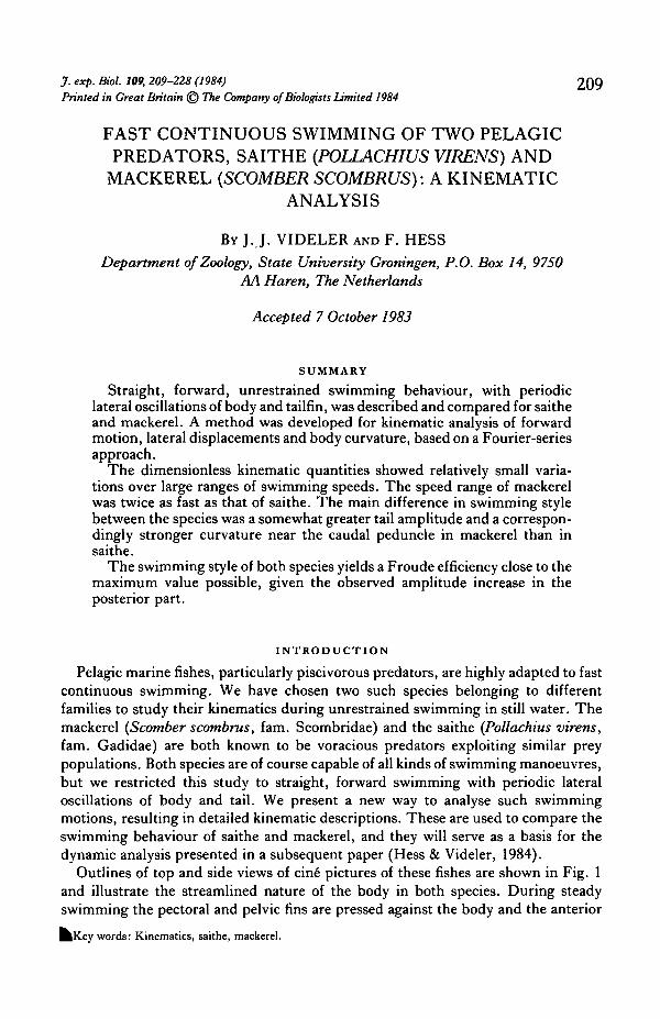
Outlines of top and side views of cin6 pictures of these fishes are shown in Fig. 1and illustrate the streamlined nature of the body in both species. During steadyswimming the pectoral and pelvic fins are pressed against the body and the anterior

^ K e y words: Kinematics, saithe, mackerel.

210 J. J. VlDELER AND F. HESS

Fig. 1. Top and side views of swimming saithe (A) and mackerel (B), drawn from cin£ film images.

parts of dorsal and anal fins are collapsed. The first dorsal fin of the mackerel fits ina groove in the back. The side views show how the last dorsal and anal fins are partlyerected and affect the shape of the fish during swimming. The similarity between thepairs of pictures is striking but the tail blades have a different shape and the caudalpeduncle of saithe is higher.

Gray (1933), using successive cine pictures of top views of swimming fish, showedthat 'waves of curvature pass along the body from head to tail', and that every point on thebody follows a wave track in space in the swimming direction at an average speed lowerthan the speed of the body wave. A precise description of these wave phenomena forswimming cod was given by Videler & Wardle (1978) and Wardle & Videler (1980a).The use of high-speed cine" film, digitizer, computer and numerical techniques allows usto carry out a more detailed kinematic analysis for saithe and mackerel.

For the comparison of swimming motions of fishes of different sizes and swimmingat different speeds it is very convenient to use dimensionless quantities. We thereforeshall use the fish length L as a unit of length and the period T as a unit of time. Theunit of velocity then becomes L/T.

METHODS

High speed films of saithe and mackerel

Saithe were trained to swim back and forth between feeding points situated at theends of a 14 m long tank at the DAF's Marine Laboratory in Aberdeen. Films of topviews of passing fish were taken with a high-speed camera mounted on a scaffoldina

Kinematic analysis of swimming 211

K)\ver over the middle of the tank* At that point the tank was l-2m wide and 0-8 meep. In our analysis we use film sequences of one specimen which was 0-35 cm long

at first and had grown to O40 cm when it was recorded again a few months later.Swimming mackerel were filmed in a 5 m long tank (1 m wide and 0*8 m deep) at

a field station of the Marine Laboratory near Loch Ewe in North West Scotland.Mackerel were caught near the station using lines fitted with unbarbed hooks. Fishwere transported in seawater-filled containers and released in the tank within a fewminutes after capture. Great care was taken not to touch the animals. Mackerel alwaysstarted to swim very fast and vigorously immediately after release. The inside of theswimming tank was lined with a plastic sheet, a few centimetres away from the wall,to avoid fatal damage from head-on collisions against the wall. After a few hours theyusually relaxed and cruised the tank continuously at more moderate speeds. Filmsequences of both types of swimming behaviour of four specimens are used in thispaper. A background illumination technique made it possible to film both species at100 or 200 frames per second without disturbing the behaviour of the fish with highlight levels. Details are given elsewhere (Videler, 1981).

We selected only those film sequences which showed regular periodic swimmingmotions, to a good approximation along a straight horizontal path. We excluded theburst and coast swimming style, frequently used by saithe (Videler & Weihs, 1982)and sometimes by mackerel. Sequences of slow swimming at velocities lower than 1-5lengths s"1 for saithe and 3 lengths s"1 for mackerel were discarded, because the fishswam with extended pectoral fins [see also Gray's (1933) example of a mackerelswimming at 12 lengths s"1].

In each sequence the head of the fish entered the field of view of the camera afterthe camera had reached its set speed of frame rate. The fish subsequently crossed thefield of view and the sequence ended when the tail tip disappeared. The camera wasfitted with a reference grid, visible on each frame, which was the earth bound frameof reference because the camera was mounted in a fixed position.

The length of the crossing fish was used to scale the pictures. We used the digitizedoutlines of whole fish images for the analysis of propulsive wave characteristics.

Swimming motion analysis

The circumference of the image of the fish on each frame and two selected pointsof the reference grid were digitized with an HP 9874A digitizer and an HP 9835Acomputer. In the tail region the outlines of the fin rays of the middle of the fin wereused even if the tailblade was dorsoventrally cambered. The coordinates of the tip ofthe head and the reference points served to calculate the mean path of motion withstandard linear regression equations. This mean path of motion was designed to bethe x-axis in a new frame of reference and all coordinates were transformed according-ly. The z-axis was perpendicular to the x-axis and horizontal. For each of the bodycircumferences a central line dividing the fish image into two lateral halves wascomputed. On the left and right outline 100 equidistant points were calculated. Pointnumber 1 on both outlines was the tip of the head and the first point on the centre line.Similarly point number 100 was the tailtip and the last point on the centre line. Theother points on the centre line were situated half way between equivalent points of theoutlines. The centre lines were divided into 99 line segments. The sum of the 99 pieces


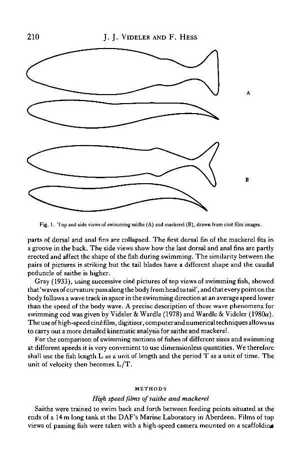
was the length of the fish which was supposed to be the same for all the images of ongsequence and equal to the average centre line length. Small deviations (<±2 %) fromthe average centre line length, mainly due to digitizing inaccuracies, were eliminatedby length corrections. Fig. 2 shows the digitized outlines and computed centre linesfor one sequence of saithe. The centre lines were used for the kinematic analysis ofthe swimming motion. This analysis deals with: the time period, the forward motion,the lateral displacement and the body curvature.

Time period

For the determination of the time period we used two methods. The first methodis rather simple. The lateral (z) position of each body point oscillates in time. The timeintervals between successive extreme lateral positions are estimates for half of the timeperiod T. The resulting values for T are averaged, after giving each one a weightproportional to the corresponding amplitude. This method can only be applied tobody points whose amplitude is greater than the noise present in the digitized data.If the film contains less than one period this method may be rather awkward. Thesecond method is more sophisticated and takes considerably more computing time.For each body point (p = 1, . . . , 100) the lateral position hp(t) as a function of timeis approximated by a function of the form:

,. . , 2jrt , . 2^rtt(t) = ao + bot — ai cos-— + bi sin—-. (1)

O l i

Pollachius virens (100 frames per second)

Fig. 2. Digitized film images of a saithe sequence (SI). Top: superimposed circumferences withcomputed centre lines. Left: the same images at half size shifted laterally for greater clarity. Right:centre lines only, with x-positions of nose made to coincide.


Khe first two terms represent a straight-line motion and the last two terms a harmonicotion. If the film frames represent the time points tj, i = 1, . . . , n, then ao, bo, ai,

bi and T must be chosen such that

DP = i { h p ( t i ) - f ( t i ) } 2 (2)

is minimized. For a chosen fixed value of T, Dp is minimized as a function of ao, ai,bo, bi. This is done by solving a 4 X 4 matrix equation. The resulting value for Dp

is a function of T only: DP(T). This function is minimized by a unidirectional searchmethod (Himmelblau, 1972). For each body point p, we obtain the correspondingoptimum value for T: T p . For any T close enough to Tp , Dp is a quadratic functionofT:

DP = AP + B P (T-T P ) 2 . (3)

The final ('best') estimate for T is found by minimizing:

100

which is the same as averaging the Tp values with suitable weights. In cases where weused both methods the results were never significantly different. The time period Twill be used as a unit of time.

Forward motion

The forward motion of the fish is approximated by a straight-line motion with aconstant acceleration or deceleration plus a speed fluctuation originating from the tailbeat. We have used the mean distance in the x-direction between nose and tail, L, asa unit of length. (This is about 1 or 2 % smaller than the length of the fish when it isstraight.) The x-length, L, is approximated by a function of the form:

f(t) = ao + a2cos2(Wt + bzsin2<wt, ft) = 2n/T . (4)

A least-squares fit yields the mean value L = ao. The two last terms represent aperiodic x-length fluctuation with period T/2.

For the forward speed of the fish we take the speed of body point number 25, as thisis close to the fish's centre of mass, but this choice is not at all critical. This point'sx-position is approximated by a function of the form:

f (t) = ao + bo(t - tc) + co(t - tc)2 + azcos2firt + b2sin2(ut, ft) = 2JT/T, (5)

where tc is the time point half way between the first and the last frame. The first threeterms represent a motion with constant acceleration, and the other two terms a period-ic fluctuation. A least-squares fit yields the following quantities. The mean forwardvelocity is bo, or dimensionless in lengths/period:

U = bo .T /L . (6)

The mean acceleration is 2co , or dimensionless in lengths/period :

U = 2c0 .T2/L (7)


and the amplitude of the periodic velocity fluctuation in lengths/period:

(8)

The observed speed fluctuations turn out to be insignificant. As for the acceleration,it is not so much U, but rather the quantity /?= U/U2 which is of hydrodynamicrelevance (Hess & Videler, 1984). j8 is the relative velocity increase during the timeit takes to move one fish length; we call it the acceleration parameter.

Lateral displacement

The bulk of the kinematic analysis concerns the lateral motion of the fish body. Inthis analysis we assume that the forward motion of all body points is uniform. Thisimplies that in the coordinate system which moves with the fish at speed U, the bodypoints move in a lateral (z) direction only. The x-component of the motion is ignored.This assumption is justified as long as the amplitudes of all body points are smallenough. In reality the situation may be somewhat different, but the differences arenever so large as to influence our conclusions. The fish stays close to the x-axis andoccupies a region between x = 0 (nose) and x = L (tail) (see Fig. 3). In terms of L,the nose is at x = 0 and the tail at x = 1. The centre line of the fish is described by theequation:

z = h(x,t). (9)

The digitized data contain values for h(x,t) at 100 body points, Xp = (p—1)/99(p = 1 100) and at certain time points, ti (i = 1, . .., n). These values containerrors. We want to obtain a smooth function h(x,t) which closely fits the data. First weconsider h(x,t) as a function of time. Since it is periodic with period T, it can berepresented by a Fourier series. We make a least-squares approximation as indicated by:

5

h(x,t) = ao(x) + bo(x) (t - tc) + I [aj(x)cosjart + bj(s)sinjan]. (10)

The first two terms represent a straight-line motion. Frequencies higher than thefifth need not be included as their contributions drown in the noise. Ideally, for each

z

U-water

Fig. 3. Coordinate system x, z. The water moves with velocity U in the x-direction.


Kjint Xp we should obtain the same ao , and bo should vanish. Moreover, because ofteral symmetry we have:

h(x,t) - ao = - [h(x,t + T/2) - ao]

and all Fourier terms with even frequencies should vanish. After the fit, we only retainthe odd Fourier terms, which constitute an idealized motion distilled from the recor-ded motion. This procedure is justified if the rejected terms are small. In the 13 filmsequences of saithe the ao values never differed by more than 0*02 L, and |bo| ^0-04L/T. The ratio between second frequency amplitude and first frequency am-plitude, a2/ai, in the tail region is =£0-03 in half of the cases, and in the worst case (S9)it reaches —0-15. The path curvature as seen from above is strongest for one mackerelsequence (M8): L/R = 0-06, where R is the path's radius. In all other selected casesit is much weaker. Thus the following approximation for h(x,t) appears to be reason-ably accurate in most of the 25 selected cases:

h(x,t) = .2 j s {aj(x)cosj(Wt + bj(x)sinja*}. (11)

For each body point we now have six Fourier coefficients, aj and bj, characterizingthe lateral motion of the fish body. Now we consider h(x,t) as a function of x. Weobtain a smooth function in x by the use of cubic splines (Ahlberg, Nilson & Walsh,1967). For each of the six Fourier coefficients a least-squares approximation in termsof cubic splines is made. The fish's centre line is divided into 20 segments by 21equidistant points (so-called knots) including nose and tail. On each of the segmentsa cubic spline is a third degree polynomial. The spline and its first and secondderivatives are continuous across the division points (knots). At the nose and tailpoints we must impose end conditions. We choose the condition of vanishingcurvature: the second derivative with respect to x must vanish: h"(x,t) = 0 at x = 0and at x = 1. This is reasonable for the nose, but what about the tail? The motionpicture images indeed show that the fish tail is far less curved at the end than nearthe caudal peduncle. As a check we made an approximation with alternative endconditions: curvature at end point equals curvature at next knot. This led to almostidentical results. A spline is completely determined by its values at the knots. Afterthe fit we obtain for each Fourier component 21 numbers representing the valuesof the coefficient at the knots Xk = (k-l) /20, k = 1, . . . , 21. Thus the lateral motionof the fish is described by a smooth function h(x,t) which is characterized by 6 X 21numbers.

The smoothing of the lateral motion, first in time by a sum of Fourier terms, thenalong the body by cubic splines, retains all the significant features and removes muchof the noise from the data. As regards the time dependence, since we include Fourierterms up to the fifth frequency, differences in h(x,t) for time points separated byintervals down to about T/20 can be taken into account. It turns out that the firstfrequency accounts for most of the lateral motion, the third frequency contributessomething in the posterior part of the fish and the fifth frequency contributions canhardly be distinguished from noise. In the smoothing by splines we used 20segments along the body, therefore differences in h(x,t) for body points separatedfcr distances down to L/20 can be taken into account. This resolution turns out to


be quite sufficient, considering the noise in the data. Taking fewer knotsremove more noise from the Fourier coefficients but might also lead to some lossinformation.

The resulting, smoothed function h(x,t) can also be written in the form:

wouUloss M

h(x,t) = . JSw hj(x)cosJQ>[t (12)

Here hj(x) is the amplitude at point x belonging to frequency j , and Tj(x) is the phasefunction; it represents the instant at which the contribution of frequency j reaches itsmaximum at x. Therefore multiples of T / j may be added to Tj(x) or subtracted fromit. T h e functions hj(x) and Tj(x) are related to the Fourier coefficients aj(x) and bj(x)by:

aj(x) = hj(x)cosj(WTj(x)bj(x) = hj(x)sinjanj(x)

j j

/ x 1 bj(x)Ti(x) = — arctan -^-f.

)O) aj(x)

}

}

(13)

The functions hj(x) and tj(x) (j = 1, 3, 5) are shown in Fig. 4 for one saithe sequence(SI). The hj values are expressed in units L, and the tj values in units T. In these unitsft) = 2.K. The origin of the time scale has been chosen to coincide with the instant ofmaximum first frequency tail point deflection: Ti(l) = 0 by definition. This conven-tion is adopted throughout this paper.

014

0 0-2 0-4 0-6 0-8 10 0 0-2 0-4 0-6 0-8 10

Fig. 4. Lateral deflection h(x,t) for saithe sequence SI. Left: amplitude curves hj(x). Right: phasecurves tj(x). For explanation see text. Drawn curves, first frequency; dashed, third frequency;stippled, fifth frequency contribution.

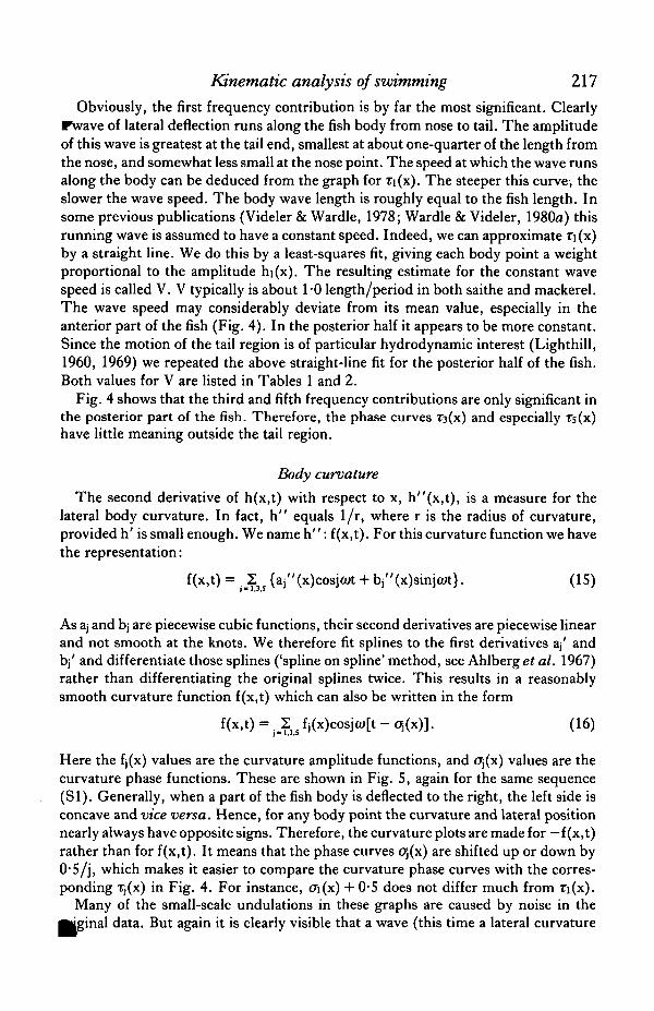
Kinematic analysis of swimming 217Obviously, the first frequency contribution is by far the most significant. Clearly

r\vave of lateral deflection runs along the fish body from nose to tail. The amplitudeof this wave is greatest at the tail end, smallest at about one-quarter of the length fromthe nose, and somewhat less small at the nose point. The speed at which the wave runsalong the body can be deduced from the graph for Ti(x). The steeper this curve, theslower the wave speed. The body wave length is roughly equal to the fish length. Insome previous publications (Videler & Wardle, 1978; Wardle & Videler, 1980a) thisrunning wave is assumed to have a constant speed. Indeed, we can approximate Ti(x)by a straight line. We do this by a least-squares fit, giving each body point a weightproportional to the amplitude hi(x). The resulting estimate for the constant wavespeed is called V. V typically is about 1*0 length/period in both saithe and mackerel.The wave speed may considerably deviate from its mean value, especially in theanterior part of the fish (Fig. 4). In the posterior half it appears to be more constant.Since the motion of the tail region is of particular hydrodynamic interest (Lighthill,1960, 1969) we repeated the above straight-line fit for the posterior half of the fish.Both values for V are listed in Tables 1 and 2.

Fig. 4 shows that the third and fifth frequency contributions are only significant inthe posterior part of the fish. Therefore, the phase curves T3(x) and especially Ts(x)have little meaning outside the tail region.

Body curvature

The second derivative of h(x,t) with respect to x, h"(x,t), is a measure for thelateral body curvature. In fact, h" equals 1/r, where r is the radius of curvature,provided h' is small enough. We name h": f(x,t). For this curvature function we havethe representation:

f(x,t) = ._2 s {aj"(x)cosj<wt + bj"(x)sinj(Ut}. (15)

As aj and bj are piecewise cubic functions, their second derivatives are piecewise linearand not smooth at the knots. We therefore fit splines to the first derivatives aj' andbj' and differentiate those splines ('spline on spline' method, see Ahlbergef al. 1967)rather than differentiating the original splines twice. This results in a reasonablysmooth curvature function f(x,t) which can also be written in the form

f(x,t) = j J2u fj(x)co8j(»[t - os(x)]. (16)

Here the fj(x) values are the curvature amplitude functions, and oj(x) values are thecurvature phase functions. These are shown in Fig. 5, again for the same sequence(SI). Generally, when a part of the fish body is deflected to the right, the left side isconcave and vice versa. Hence, for any body point the curvature and lateral positionnearly always have opposite signs. Therefore, the curvature plots are made for —f (x,t)rather than for f(x,t). It means that the phase curves Oj(x) are shifted up or down by0-5/j, which makes it easier to compare the curvature phase curves with the corres-ponding Tj(x) in Fig. 4. For instance, 0i(x) + 0*5 does not differ much from Ti(x).

Many of the small-scale undulations in these graphs are caused by noise in the•Hginal data. But again it is clearly visible that a wave (this time a lateral curvature

J . J . VlDELER AND F . HESS

0-2

0 0-2 0-4 0-6 0-8 10

Fig. 5. Body curvature —f(x,t) for saithe sequence SI. Left: amplitude curves. Right: phase curves.'For explanation see text. Drawn curves, first frequency; dashed, third frequency; stippled, fifthfrequency contribution.

wave) runs from the anterior part of the body to the tail. The amplitude is greatestjust behind the caudal peduncle, i.e. in the anterior part of the tail, where is reachesa value of about 4. The radius of curvature r in this region can become as small asL/4. The front part of the fish hardly bends at all, and the curvature as drawn in Fig. 5represents more noise than real bending. Therefore, the phase curves have no physicalmeaning in the anterior 25 % of the length of the fish, and for the higher frequenciesprobably the anterior 75 %.

RESULTS AND DISCUSSION

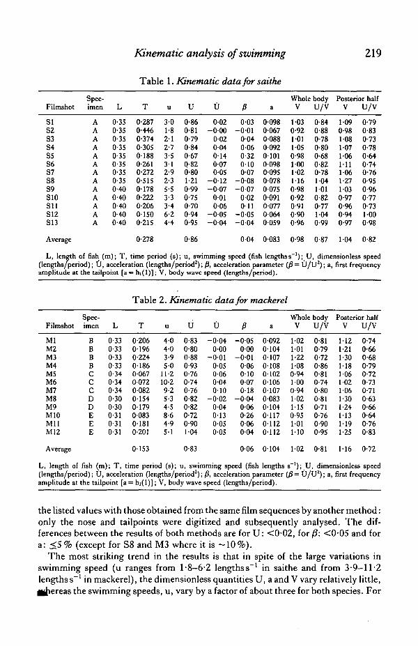
Kinematic quantities derived from each film sequence are given for saithe in Table1 and for mackerel in Table 2. The columns of these tables contain, from left to right:the name of the film sequence, the fish specimen, the length of the fish L in metres,the time period T in seconds, the swimming speed u in fish lengths per second, thedimensionless speed U in lengths/period, the acceleration U in lengths/period2, theacceleration parameter /? = U/U2, the first frequency amplitude at the tailpoint a =hi(l) in lengths, the body wave speed V in lengths/period as obtained from a straight-line fit over the whole fish body, the ratio U/V, and again V and U/V, but now forthe posterior half of the fish only. The bottom line of each table gives values for the'average' saithe and the 'average' mackerel. The meaning of 'average' will be explainedbelow.

Before discussing the results it is useful to consider the accuracy of these data. Theperiod T has an accuracy of about 1 %. For the quantities U, U and a we compared


Table 1. Kinematic data for saithe

Filmshot

SIS2S3S4SSS6S7S8S9S10Sl lS12S13

Spec-imen

AAAAAAAAAAAAA

L

0-350-350-350-350-350-350-350-350400-400-400-400-40

T

0-2870-4460-3740-30501880-2610-2720-5150-1780-2220-20601500-215

u

3-01-82 12-73-53 12-92-35-53-33-46-24-4

U

0-860-810-790-840-670-826-801-210-990-750-700-940-95

U

0-02- 0 0 0

0-020-040140-070-05

- 0 1 2- 0 0 7

0010-06

-0-05- 0 0 4

P0-03

-0-010040-060-32010007

- 0 0 8-0-07

002O i l

-0-05- 0 0 4

a

0-0980-0670-088009201010-098009500780-0750-0910-07700640059

Whole bodyV

1-030-921011-050-981001021160-980-920-910-900-96

U/V

0-840-880-780-800-680-820-781041010-820-771-040-99

Posterior halfV

1090-981-081-07106•11

1-061-27

030-970-960-94()-97

U/V

0-790-830-730-780-640-740-760-950-960-770-731-000-98

Average 0-278 0-86 004 0083 0-98 0-87 104 0-82

L, length of fish (m); T, time period (s); u, swimming speed (fish lengthss ' ) ; U, dimensionless speed(lengths/period); U, acceleration (lengths/period2); jS, acceleration parameter (|8 = U/U 2) ; a, first frequencyamplitude at the tailpoint [a = hi(l)]; V, body wave speed (lengths/period).

Filmshot

MlM2M3M4M5M6M7M8M9M10MilM12

Spec-imen

BBBBCCCDDEEE

L

0-330-330-330-330-340-340-340-300-300-310-310-31

Table

T

020601960-22401860-0670072008201540-179008301810-201

2. Kinematic data for mackerel

u

4-04-03-95 0

11-210-29-25-34-58-64-95-1

U

0-830-800-880-930-760-740-760-820-820-720-901-04

U

-0-040-00

- 0 0 10-050-060-040-10

- 0 0 20-040-130050-05

P- 0 0 5

000-0-01

006010007018

- 0 0 40060-260060-04

a

0-09201040-107010801020106010700830-104011701120-112

Whole bodyV

1021011-221080-941-000-941021-150-95101110

U/V

0-810-790-720-860-810-740-800-810-710-760-900-95

Posterior halfV

1-121-211-301-181061021061-301-241131191-25

U/V

0-740-660-680-790-720-730-710-630-660-640-760-83

Average 0-153 0-83 0-06 0104 102 0-81 1-16 0-72

L, length of fish (m); T, time period (s); u, swimming speed (fish lengths s ' ) ; U, dimensionless speed(lengths/period); U, acceleration (lengths/period2); /S, acceleration parameter (/?= U/U2); a, first frequencyamplitude at the tailpoint [a = hi(l)]; V, body wave speed (lengths/period).

the listed values with those obtained from the same film sequences by another method:only the nose and tailpoints were digitized and subsequently analysed. The dif-ferences between the results of both methods are for U: <0-02, for/J: <0-05 and fora: <5 % (except for S8 and M3 where it is -10%) .

The most striking trend in the results is that in spite of the large variations inswimming speed (u ranges from 1-8-6-2 lengths s"1 in saithe and from 3-9-11-2lengths s"1 in mackerel), the dimensionless quantities U, a and V vary relatively little,^jhereas the swimming speeds, u, vary by a factor of about three for both species. For


saithe U lies between 0-70 and 1-21 (factor 1-7), V (posterior half) between 0-94 an41-27 (factor 1-4), U/V between 0-64 and 1-00 (factor 1-6), and a between 0-059 an™0-101 (factor 1-7). For mackerel U lies between 0-72 and l-04(factor 1-4), Vbetween1-02 and 1-30 (factor 1-3), U/V between 0-63 and 0-83 (factor 1-3) and a between0-083 and 0-117 (factor 1-4). In the case of mackerel such variations may be partly dueto differences in swimming style between individual specimens. However, it appearsthat both species have a swimming style which stays roughly the same through a widerange of speeds.

A quantity mentioned before, but not listed in the tables is AU, the amplitude ofthe periodic speed fluctuations. For the saithe film sequences it lies between 1 and 5 %of U. (The 5% case is S5, which has the greatest acceleration.) But if the phaserelationship with the tail position is taken into account, these fluctuations yield anaverage amplitude of only 0-6 % of U for the 13 cases, which is negligible. Consideringthe estimated accuracy of our results, we conclude that the periodic speed fluctuations,in as far as they are correlated with tailbeat, are smaller than 2 % for saithe. For mackerelwe did not actually calculate the average, but the situation appears to be the same.

Comparison of swimming styles

In the analysed sequences the lowest and highest swimming speeds of mackerel areabout twice as high as those of saithe. Data from the literature indicate that the speedranges presented here give a good impression of the capabilities of the two species.Our maximum velocity for saithe of 6-2 lengths s"1 is very close to the maximum burstswimming speed of 6 4 lengths s"1 recorded by Blaxter & Dickson (1959). We obser-ved steady swimming without the use of pectoral fins at velocities higher than 1-5lengths s"1, which is half the maximum sustained cruising speed of saithe found byGreer Walker & Pull (1973). Wardle (1979) recorded a minimum muscle contractiontime for a 0-35-m mackerel of about 0-03 s, which would give T = 0-06 s, correspond-ing to our fastest mackerel in sequence M5 (see also Wardle & Videler, 19806).

Let us now consider more closely the similarities and differences between theanalysed cases. For both saithe and mackerel u appears to be proportional to 1/T(which implies that U does not vary much) (Fig. 6A). Such a linear relationship wasfirst found by Bainbridge (1958). Indeed, we would theoretically expect (ignoringviscous effects) that a fish can maintain exactly the same swimming style at all swim-ming speeds, in other words, that the dimensionless quantities remain the same, allvelocities (in the fish body as well as in the water) scaling up or down with the tailbeatfrequency.

The variations showing up in Tables 1 and 2 may be partially due to differences inacceleration. Fig. 6 (B, C, D) contains plots for U, U/V and a against the accelerationparameter /?. We see that for both saithe and mackerel there is a trend of U decreasingwith increasing /?, as expected. A similar trend is found for U/V, but only with saithe.The tail amplitude (a) increases with /? for both species; a seems to be more stronglycorrelated with acceleration (j8) than with actual swimming speed u, as indicated byFig. 6E. For both saithe and mackerel, the wave speed V (posterior half) shows apositive correlation with the period T (Fig. 6F). Regression lines have not been drawnin the graphs, but we list them here with the correlation coefficients between brackets.(T is in seconds, u in lengths s"1 and the other quantities are dimensionless.)


Saithe Mackerel

u = - 0-03 + 0-85 '/T (+0-91) u = 1-08 + 0-66 '/T (+0-99)U = 0-90 - 1-01/3 (-0-76) U = 0-86 - 0-440 (-0-42)

U/V = 0-86 - 0-94)8 (-0-86) U/V = 0-72 - 0-06/3 (-0-09)a = 0-080 + 0-086/8 (+0-64) a = 0-100 + 0-068/8 (+0-65)a = 0-099 - 0-0047u (-0-43) a = 0-100+ 0-0067u (+0-19)V = 0-90 + 0-54T (+0-66) V = 0-99 + 1-21T (+0-76)

These regression lines should be considered with caution, as the scatter in the data isrelatively large.

From Tables 1 and 2 and also from Fig. 6 it is obvious that there is an overlapbetween the data for saithe and for mackerel. This is clearly visible in Fig. 7, in whichthe first frequency lateral displacement functions hi(x) and Ti(x) are drawn for fourcases: SI, S3, M2 and M12. The differences between saithe and mackerel do notappear to be significantly greater than the differences between sequences of the samespecies. What then is the difference in swimming style between saithe and mackerel?

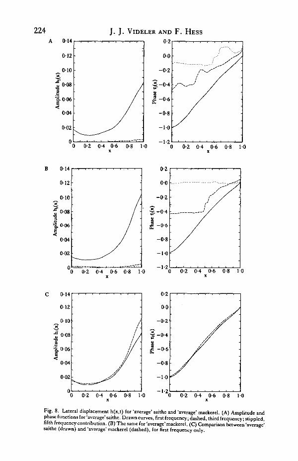
To answer this question we constructed an 'average' saithe and an 'average'mackerel as follows. For each species separately the smoothed lateral displacementfunctions h(x,t) from all sequences were averaged. Before averaging, the point t = 0was made to coincide with the instant of maximum first frequency tail point deflectionas mentioned before. Since a part of the variation in h(x,t) between the sequences isdue to errors in the data, the averaged h(x,t) is smoother. In particular the noise inthe third and fifth frequency contributions is much reduced. The results for bothsaithe and mackerel are shown in Fig. 8 for the lateral displacement and in Fig. 9 forthe curvature function —f(x,t). The bottom lines in Tables 1 and 2 list the valuesfound for a and V. The values for T, U and )8 are obtained by averaging the valuesof the individual cases. From this follows U/V.

Figs 8 and 9 show very clearly that there is a remarkable similarity between theswimming of saithe and mackerel. The tail amplitude is somewhat greater inmackerel, and the curvature near the caudal peduncle is correspondingly stronger inmackerel than in saithe. Otherwise the lateral bending in both fish appears to be thesame. The difference in the average acceleration parameter /? is far too small to explainthe difference in amplitude a. As noted before, the 'average' mackerel swims almosttwice as fast as the 'average' saithe. This is the most obvious difference between thespecies.

It appears that saithe and mackerel have nearly the same swimming style. The maindifferences found concern the tail amplitude, which is about 25 % greater in mackerelthan in saithe, and the wave speed V in the posterior half of the body, which inmackerel is about 10 % greater than in saithe. As in both species U varies around anaverage value of roughly 0-85, the ratio U/V is smaller on average in mackerel (0-72)than in saithe (0-82).

In nearly all film sequences for both saithe and mackerel, the third frequencycontribution at the tail reaches its maximum just after the first frequency contribution*Loes, the phase difference typically amounting to slightly less than 0-1T. This deviation

8 EXB 1O9

222

16 r

12

d 8

3

0


A 1-3 r

1-1

J 0-9

0

1-3 r

1-1

r0-9

0-7

0-7

OS

+ * ** +

*

4 8 12 16 - 0 1 - 0 0 1 0-2 0-31/T (Hz) fi

c oi3 r D

. * *

0 01

P

O i l

009

007

0-05

+ ++ ++

+ +

+ * **

0-2 0-3 - 0 1 0 0 1 0-2 0-3P

013

O i l

-009

007

0-05

1-3

11

*#

* « +

4 8 12ML."1)

0-7

OS

+ +

++ * * !

16 0 0-2 0-4 0-6 0-8T(s)

Fig. 6. Some kinematic data for saithe (•) and mackerel (+). (A) Swimming speed u (Ls ') vstailbeat frequency 1/T (s"1). (B) Dimensionless swimming speed U (LT"1) vs accelerationparameter /S. (C) U/V (posterior half) vs /3. (D) First frequency tailpoint amplitude a (L) vs /3. (E)a (L) vs u (Ls"1). (F) Body wave speed (posterior half) V (LT"1) vs period T (s).


014

0 1 2 -

0

Fig. 7. Lateral displacement (first frequency contribution only) for two saithe and two mackerel,taken as representative examples. Left: amplitude functions h|(x). Right: phase functions Ti(x). Forexplanation see text. Drawn curves are for saithe (SI, S2), dashed curves for mackerel.

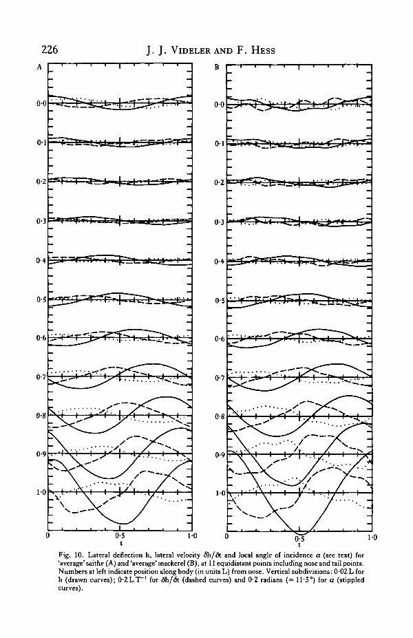
from a pure sinusoidal motion is more easily seen in Fig. 10. Here, for 11 equidistantpoints on the body of 'average' saithe (Fig. 10A) and mackerel (Fig. 10B), the lateraldeflection h(x,t) is plotted as a function of time during one period. In addition, thelateral velocity 6h/<5t is shown. The tailpoints reach their maximum velocity justbefore they cross the plane z = 0. The third quantity plotted is the local angle ofincidence Cf(x,t), which is the angle between the fish's centre line and the local direc-tion of motion. It is derived from h(x,t) as follows:

(17)<5h/(5x =6h/6t = Utani/;

The angle 8 between centre line and the x-axis does not exceed ±30°

EfficiencyAlthough this paper deals with kinematics rather than dynamics, it seems

appropriate at this point to make a simple estimate for the hydrodynamic efficiency.We use formula (8) from Lighthill's (1960) paper on small-amplitude slender-bodytheory as a starting point. The Froude efficiency is the ratio between the useful workand the total mechanical work done by the fish, the useful work being the total workminus the kinetic energy imparted to the water. Let us ignore the higher frequencycontributions, and let V be the body wave speed in the tail region: Ti(x) = (x - 1)/V.Then we have for the function h(x,t) in the tail region:

) (18)

224 J . J . VlDELER AND F . HESS

0-2

0 0-2 0-4 0-6 0-8 10 0 0-2 0-4 0-6 0-8 10

0 0-2 0-4 0-6 0-8 100 0-2 0-4 0-6 0-8 1

0 0-2 0-4 0-6 0-8 10 0 0-2 0-4 0-6 0-8 10

Fig. 8. Lateral displacement h(x,t) for 'average' saithe and 'average' mackerel. (A) Amplitude andphase functions for 'average' saithe. Drawn curves, first frequency; dashed, third frequency; stippled,fifth frequency contribution. (B) The same for 'average' mackerel. (C) Comparison between 'average'saithe (drawn) and 'average' mackerel (dashed), for first frequency only.


0 0-2 0-4 0-6 0-8

o

+

0 0-2 0-4 0-6 0-8 10

0 0-2 0-4 0-6 0-8 10 0 0-2 0-4 0-6 0-8 10

Fig. 9. Body curvature — f(x,t) for 'average' saithe and 'average' mackerel. (A) Amplitude and phasefunctions for 'average' saithe. Drawn curves, first frequency; dashed, third frequency; stippled, fifthfrequency contribution. (B) The same for 'average' mackerel. (C) Comparison between 'average'saithe (drawn) and 'average' mackerel (dashed), for first frequency only.

226

00

0 1

0-2

0-3

0-4

0-5

0-6

0-7

0-8

0-9

1-0


B

oo

01

0-2

0-3

i . > ""V t̂̂ a T*->-j .-KN

—I >' I >\S\—I > O

0-4

0-5

0-6

0-7

0-8

0-9

10

0-5t

1-0 0 OSt

10

Fig. 10. Lateral deflection h, lateral velocity 6h/<5t and local angle of incidence a (see text) for'average' saithe (A) and 'average' mackerel (B), at 11 equidistant points including nose and tail points.Numbers at left indicate position along body (in units L) from nose. Vertical subdivisions: 0-02 L forh (drawn curves); 0-2LT"1 for <5h/6t (dashed curves) and 0-2 radians (= 11-5°) for a (stippledcurves).

Kinematic analysis of swimming 227iFor this lateral motion the Froude efficiency is found to be [see Lighthill, 1960,-lormulae (13) and (14)]:

r,= 1/2(1 + U/V)- 1/2 r L

where (19)

4 2;rh1(l)

If the amplitude hi(x) is constant near x = 1, then q vanishes and only the first termin (19) is left. [In several articles on the swimming of fish (e.g. Webb, 1975; Videler& Wardle, 1978) this term is used as an expression for the 'propeller efficiency'.]

For fixed q, 7] reaches its maximum value, 1 — |q|, if U/V = 1 — |q|. According toFig. 8 we have for both saithe and mackerel: h'(l)/h(l) = 2, and U^O-8, henceq = 0-25. Under these conditions the maximum Froude efficiency is r] — 0-75 forU/V = 0-75, and ??>0-70 as long as U/V lies between 0-54 and 0-86.

All mackerel sequences have U/V values within this range, and only in four casesof decelerating saithe is U/V outside this range (nearly 1*0). It appears therefore that,given the observed amplitude increase in the posterior part, the swimming style ofsaithe and mackerel yields a Froude efficiency which is close to the maximum possiblevalue.

A Royal Society Fellowship to JJV made collection of the filmed data possible inclose stimulating cooperation with Dr C. S. Wardle (Marine Laboratory Aberdeen).Cooperation with Dr Aenea Reid (Aberdeen University Computer Centre) in anearlier stage of this work is gratefully acknowledged. Mrs Hanneke Videler-Verheijenwas responsible for the painstaking steps between film frames and computer. TheFoundation for Fundamental Biological Research (BION), an organization sub-sidized by the Netherlands Organization for the Advancement of Pure Research(ZWO), financed the cooperation between the authors.

R E F E R E N C E S

AHLBERG, J. H., NILSON, E. N. & WALSH, J. L. (1967). The Theory of Splines and their Applications. NewYork, London: Academic Press.

BAINBRIDGE, R. (1958). The speed of swimming of fish as related to size and to the frequency and amplitudeof tail beat. J exp. Biol. 35, 109-133.

BLAXTER, J. H. S. & DICKSON, W. (1959). Observations on swimming speeds of fish. J . Cons. perm. int. Explor.Mer 24, 472-479.

GRAY, J. (1933). Studies in animal locomotion. I. The movement of fish with special reference to the eel. J. exp.Biol. 10, 88-104.

GREER WALKER, M. & PULL, G. (1973). Skeletal muscle function and sustained swimming speeds in the coalfish (Gadus virens L.). Comp. Biochem. Physiol. 44A, 495-501.

HESS, F. & VIDELER, J. J. (1984). Fast continuous swimming of saithe (Pollachius virens): a dynamic analysisof bending moments and muscle power. J . exp. Biol. 109, 229-251.

HIMMELBLAU, D. M. (1972). Applied non-linear Programming. New York: McGraw.LIGHTHILL, M. J. (1960). Note on the swimming of slender fish. J. FluidMech. 9, 305-317.LIGHTHILL, M. J. (1969). Hydromechanics of aquatic animal propulsion. Ann. Wet;. Fluid Mech. 44, 265-301.VIDELER, J. J. (1981). Swimming movements, body structure and propulsion in Cod (Gadus morhua). In

Vertebrate Locomotion, (ed. M. H. Day). Symp. Zool. Soc. Land. 48, 1-27. London: Academic Press.VIDELER, J. J. & WARDLE, C. S. (1978). New kinematic data from high speed cine film recordings of swimming

Cod (Gadus morhua). Neth.J. Zool. 28, 465-484.


VIDELER, J. J. & WEIHS, D. (1982). Energetic advantages of burst-and-coast swimming of fish at high speedyJ. exp. Biol. 97, 169-178.

WARDLE, C. S. (1979). Effects of temperature on the maximum swimming speed of fishes. In EnvironmentalPhysiology of Fishes, (ed. M. A. Ali). NATO advanced Study Inst. Ser. A. 35, 519-531.

WARDLE, C. S. & VIDELER, J. J. (1980a). Fish swimming. In Aspects of Animal Movement, (eds H. T. Elder& E. R. Trueman). Soc. exp. Biol. Symp. 5, 125-150. Cambridge: Cambridge University Press.

WARDLE, C. S. & VIDELER, J. J. (19806). How do fish break the speed limit? Nature, bond. 284, 445-447.WEBB, P. W. (1975). Hydrodynamics and energetics of fish propulsion. Bull. Fish. Res. Bd Can. 190, 1-159.

FAST CONTINUOUS SWIMMING OF TWO PELAGIC …jeb.biologists.org/content/jexbio/109/1/209.full.pdfFAST CONTINUOUS SWIMMING OF TWO PELAGIC PREDATORS, SAITHE ... Both species are o f course

Documents