Fast Computation of the Median by Successive Binning

8/4/2019 Fast Computation of the Median by Successive Binning

http://slidepdf.com/reader/full/fast-computation-of-the-median-by-successive-binning 1/15

Fast Computation of the Median by Successive Binning

Ryan J. TibshiraniDept. of Statistics, Stanford University, Stanford, CA 94305

email: [email protected]

October 2008

Abstract

In many important problems, one uses the median instead of the mean to estimatea population’s center, since the former is more robust. But in general, computing themedian is considerably slower than the standard mean calculation, and a fast medianalgorithm is of interest. The fastest existing algorithm is quickselect. We investigate anovel algorithm binmedian, which has O(n) average complexity. The algorithm uses arecursive binning scheme and relies on the fact that the median and mean are always atmost one standard deviation apart. We also propose a related median approximationalgorithm binapprox, which has O(n) worst-case complexity. These algorithms are highlycompetitive with quickselect when computing the median of a single data set, but aresignificantly faster in updating the median when more data is added.

1 Introduction

In many applications it is useful to use the median instead of the mean to measure thecenter of a population. Such applications include, but are in no way limited to: biologicalsciences; computational finance; image processing; and optimization problems. Essentially,one uses the median because it is not sensitive to outliers, but this robustness comes ata price: computing the median takes much longer than computing the mean. Sometimesone finds the median as a step in a larger iterative process (like in many optimizationalgorithms), and this step is the bottleneck. Still, in other problems (like those in biologicalapplications), one finds the median of a data set and then data is added or subtracted. Inorder to find the new median, one must recompute the median in the usual way, because

the standard median algorithm cannot utilize previous work to shortcut this computation.This brute-force method leaves much to be desired.

We propose a new median algorithm binmedian, which uses buckets or “bins” to recur-sively winnow the set of the data points that could possibly be the median. Because thesebins preserve some information about the original data set, the binmedian algorithm can use

1



previous computational work to effectively update the median, given more (or less) data.

For situations in which an exact median is not required, binmedian gives rise to an approx-imate median algorithm binapprox, which rapidly computes the median to within a smallmargin of error. We compare binmedian and binapprox to quickselect, the fastest existingalgorithm for computing the median. We first describe each algorithm in detail, beginningwith quickselect.

2 Quickselect

2.1 The quickselect algorithm

Quickselect (Floyd & Rivest 1975a ) is not just used to compute the median, but is a moregeneral algorithm to select the kth smallest element out of an array of n elements. (Whenn is odd the median is the kth smallest with k = (n + 1)/2, and when n is even it is themean of the elements k = n/2 and k = n/2 + 1.) The algorithm is derived from quicksort

(Hoare 1961), the well-known sorting algorithm. First it chooses a “pivot” element p fromthe array, and rearranges (“partitions”) the array so that all elements less than p are toits left, and all elements greater than p are to its right. (The elements equal to p go oneither side). Then it recurses on the left or right subarray, depending on where the medianelement lies. In pseudo-code:

Quickselect(A, k):

1. Given an array A, choose a pivot element p

2. Partition A around p; let A1, A2, A3 be the subarrays of points <, =, > p

3. If k ≤ len(A1): return Quickselect(A1, k)

4. Else if k > len(A1) + len(A2): return Quickselect(A3, k − len(A1)− len(A2))

5. Else: return p

The fastest implementations of quickselect perform the steps 3 and 4 iteratively (notrecursively), and use a standard in-place partitioning method for step 2. On the otherhand, there isn’t a universally accepted strategy for choosing the pivot p in step 1. For thecomparisons in sections 5 and 6, we use a very fast Fortran implementation of quickselect

taken from Press, Teukolsky, Vetterling & Flannery (1992). It chooses the pivot p to be themedian of the bottom, middle, and top elements in the array.

2



2.2 Strengths and weaknesses of quickselect

There are many advantages to quickselect. Not only does it run very fast in practice, butwhen the pivot is chosen randomly from the array, quickselect has O(n) average computa-tional complexity (Floyd & Rivest 1975b). Another desirable property is that uses only O(1)space, meaning that the amount of extra memory it needs doesn’t depend on the input size.Perhaps the most underappreciated strength of quickselect is its simplicity. The algorithm’sstrategy is quite easy to understand, and the best implementations are only about 30 lineslong.

One disadvantage of quickselect is that it rearranges the array for its own computationalconvenience, necessitated by the use of in-place partitioning. This seemingly innocuous side-effect can be a problem when maintaining the array order is important (for example, whenone wants to find the median of a column of a matrix). To resolve this problem, quickselect

must make a copy of this array, and use this scratch copy to do its computations (in whichcase it uses O(n) space).

But the biggest weakness of quickselect is that it is not well-suited to problems wherethe median needs to be updated with the addition of more data. Though it is able toefficiently compute the median from an in-memory array, its strategy is not conducive tosaving intermediate results. Therefore, if data is appended to this array, we have no choicewith quickselect but to compute the median in the usual way, and hence repeat much of our previous work. This will be our focus in section 6, where we will give an extension of binmedian that is able to deal with this update problem effectively.

3 Binmedian

3.1 The binmedian algorithm

First we give a useful lemma:

Lemma 1. If X is a random variable having mean µ, variance σ2, and median m, then m ∈ [µ− σ, µ + σ].

Proof. Consider

|µ −m| = |E(X −m)|≤ E|X −m|

≤ E|X − µ|= E

(X − µ)2

≤

E(X − µ)2

= σ.

3



Here the first inequality is due to Jensen’s inequality, and the second inequality is due to

the fact that the median minimizes the function G(a) = E|X − a|. The third inequality isdue to the concave version of Jensen’s inequality.

Given data p oints x1, . . . xn and assuming that n is odd1, the basic strategy of thebinmedian algorithm is:

1. Compute the mean µ and standard deviation σ

2. Form B bins across [µ − σ, µ + σ], map each data point to a bin

3. Find the bin b that contains the median

4. Recurse on the set of points mapped to b

Here B is a fixed constant, and in step 2 we consider B equally spaced bins across [µ −σ, µ + σ]. That is, we consider intervals of the form

µ− σ +

i

B· 2σ,

i + 1

B· 2σ

for i = 0, 1, . . . B − 1. Iterating over the data x1, . . . xn, we count how many points lie ineach one of these bins, and how many points lie to the left of these bins. We denote thesecounts by N i and N L.

In step 3, to find the median bin we simply start adding up the counts from the leftuntil the total is ≥ (n + 1)/2. That is, b is minimal such that

N L +b

i=0

N i ≥ n + 1

2.

Note that Lemma 1 guarantees that b ∈ {0, . . . B − 1}.Finally, in step 4 we iterate through x1, . . . xn once again to determine which points were

mapped to bin b. Then we consider B equally spaced bins across µ−σ +bB· 2σ, b+1

B· 2σ

,and continue as before (except that now N L is the number of points to the left of themedian bin, i.e. N L ← N L +

b−1i=0 N i). We stop when there is only one point left in the

median bin—this point is the median. (In practice, it is actually faster to stop when theremaining number of points in the median bin is ≤ C , another fixed constant, and then find

the median directly using insertion sort.)1An analogous strategy holds when n is even. Now at each stage we have to keep track of the bin that

contains the “left” median (the kth smallest element with k = n/2) and the bin that contains the “right”median (k = n/2 + 1). This is more tedious than the odd case, but is conceptually the same, so hereafterwe’ll assume that n is odd whenever we talk about binmedian.

4



Notice that a larger value of B gives fewer points that map to the median bin, but it

also means more work to find b at each recursive step. For the time trials in sections 5and 6, we choose B = 1000 because it weighs these two factors nicely. We also replace therecursive step with an iterative loop, and use C = 20. Binmedian is implemented in Fortranfor the time trials, and this code, as well as an equivalent implementation in C, is availableat http://stat.stanford.edu/~ryantibs/median/.

3.2 Strengths and weaknesses of binmedian

Beginning with its weaknesses, the binmedian algorithm will run faster with fewer pointsin the median’s bin, and therefore its runtime is necessarily dependent on the distributionof the input data. The worst case for binmedian is when there is a huge cluster of pointssurrounding the median, with a very large standard deviation. With enough outliers, the

median’s bin could be swamped with points for many iterations.However, we can show that the algorithm’s asymptotic running time is largely unaffected

by this problem: with very reasonable assumptions on the data’s distribution, binmedian

has O(n) average complexity (see A.1). Moreover, this robustness also seems to be true inpractice. As we shall see in section 5, the algorithm’s runtime is only moderately affectedby unfavorable distributions, and in fact, binmedian is highly competitive with quickselect

in terms of running time.Like quickselect, the binmedian algorithm uses O(1) space, but (like quickselect) this

requires it to change the order of the input data. The greatest strength of binmedian is thatthe algorithm is able to quickly cache some information about the input data, when it mapsthe data points to bins. This gives rise to a fast median approximation algorithm, binapprox.

It also enables binmedian, as well as binapprox, to efficiently recompute the median when weare given more data. We’ll see this in section 6, but first we discuss binapprox in the nextsection.

4 Binapprox

4.1 The binapprox algorithm

In some situations, we do not need to compute the median exactly, and care more aboutgetting a quick approximation. Binapprox is a simple approximation algorithm derived frombinmedian. It follows the same steps as binmedian, except that it stops once it has computed

the median bin b, and just returns the midpoint of this interval. Hence to be p erfectly clear,the algorithm’s steps are:

1. Compute the mean µ and standard deviation σ

2. Form B bins across [µ − σ, µ + σ], map each data point to a bin

5



3. Find the bin b that contains the median

4. Return the midpoint of bin b

The median can differ from this midpoint by at most 1/2 the width of the interval, or1/2 · 2σ/B = σ/B. Since we use B = 1000 in practice, binapprox is accurate to within1/1000th of a standard deviation.

Again, we implement binapprox in Fortran for sections 5 and 6. This code as well as Ccode for binapprox is available at http://stat.stanford.edu/~ryantibs/median/.

4.2 Strengths and weaknesses of binapprox

Unlike binmedian, the runtime of binapprox doesn’t depend on the data’s distribution, since

it doesn’t perform the recursive step. It requires O(1) space, and doesn’t perturb the inputdata, so rearranging is never a problem. The algorithm has O(n) worst-case computationalcomplexity, as it only needs 3 passes through the data. It consistently runs faster thanquickselect and binmedian in practice. Most importantly it extends to a very fast algorithmto deal with the update problem.

Binapprox’s main weakness is fairly obvious: if the standard deviation is extremely large,the reported approximation could be significantly different from the actual median.

5 Speed comparisons on single data sets

We compare quickselect, binmedian, and binapprox across data sets coming from various

distributions. For each data set we perform a sort and take the middle element, and reportthese runtimes as a reference point for the slowest way to compute the median.We test a total of eight distributions. The first four—uniform over [0, 1], normal with

µ = 0, σ = 1, exponential with λ = 1, chi-square with k = 5—are included because they arefundamental, and frequently occur in practice. The last four are mixed distributions thatare purposely unfavorable for the binmedian algorithm. They have a lot of points aroundthe median, and a huge standard deviation. Two of these are mixtures of standard normaldata and uniformly distributed data over [−103, 103], resp. [−104, 104]. The other two aremixtures of standard normal data and exponential data with λ = 10−3, resp. λ = 10−4.All these mixtures are even, meaning that an equal number of points come from each of thetwo distributions. Table 1 gives the results of all these timings, which were performed onan Intel Xeon 64 bit, 3.00GHz processor.

For the first four distributions, quickselect and binmedian are very competitive in terms of runtime, with quickselect doing better on the data from U (0, 1) and N (0, 1), and binmedian

doing better on the data from E (1) and χ25. It makes sense that binmedian does well on the

data drawn from E (1) and χ25, upon examining the probability density functions of these

6





distributions. The density function of the exponential distribution, for example, is at its

highest at 0 and declines quickly, remaining in sharp decline around the median (log 2/λ).This implies that there will be (relatively) few points in the median’s bin, so binmedian getsoff to a good start.

Generally speaking, binmedian runs slower than quickselect over the last four distribu-tions. But considering that these distributions are intended to mimic binmedian’s degeneratecase (and are extreme examples, at that), the results are not too dramatic at all. The bin-

median algorithm does worse with the normal/uniform mixtures (skewed on both sides)than it does with the normal/exponential mixtures (skewed on one side). At its worst,binmedian is 1.3 times slower than quickselect (130.9 versus 101 ms, on the N (0, 1) andU (−104, 104) mixture), but is actually slightly faster than quickselect on the N (0, 1) andE (10−3) mixture.

Binapproxis the fastest algorithm across every distribution. It maintains a reasonablemargin on quickselect and binmedian (up to 1.62 and 1.69 times faster, respectively), though

the differences are not striking. In the next section, we focus on the median update problem,where binmedian and binapprox display a definite advantage.

6 Speed comparisons on the update problem

Suppose that we compute the median of some data x1, . . . xn0 , and then we’re given moredata xn0+1, . . . xn, and we’re asked for the median of the aggregate data set x1, . . . xn. Of course we could just go ahead and compute the median of x1, . . . xn directly, but then wewould be redoing much of our previous work to find the median of x1, . . . xn0. We’d like a

better strategy for updating the median.Consider the following: we use binmedian to compute the median of x1, . . . xn0 , and savethe bin counts N i, i = 0, . . . B − 1, and N L, from the first iteration. We also need save themean µ0 and the standard deviation σ0. Given xn0+1, . . . xn, we map these points to theoriginal B bins and just increment the appropriate counts. Then we compute the medianbin in the usual way: start adding N L + N 0 + N 1 + . . . and stop when this is ≥ (n + 1)/2.

But now, since we haven’t mapped the data x1, . . . xn to bins over its proper mean andstandard deviation, we aren’t guaranteed that the median lies in one of the bins. In thecase that the median lies to the left of our bins (i.e. N L ≥ (n + 1)/2) or to the right of ourbins (i.e. N L + N 0 + . . . N B−1 < (n + 1)/2), we have to start all over again and perform theusual binmedian algorithm on x1, . . . xn. But if the median does lie in one of the bins, thenwe can continue onto the second iteration as usual. This can provide a dramatic savings intime, because we didn’t even have to touch x1, . . . xn0 in the first iteration.

We can use binapprox in a similar way: save µ0, σ0, N i, N L from the median computationon x1, . . . xn0, and then use them to map xn0+1, . . . xn. We then determine where the medianlies: if it lies outside of the bins, we perform the usual binapprox on x1, . . . xn. Otherwise

8



we can just return midpoint of the median’s bin.

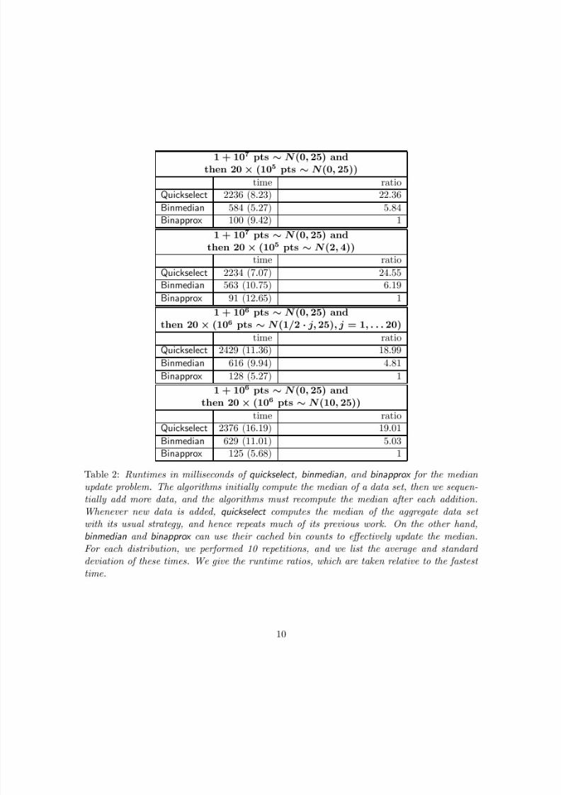
In this same situation, quickselect does not have a way to save its previous work, and mustredo the whole computation.2 In table 2, we demonstrate the effectiveness of binmedian andbinapprox on this update problem. Instead of adding data xn0+1, . . . xn only once, we add itmany times, and we record how long it takes for the algorithms to compute these mediansin one contiguous block. Binmedian and binapprox each keep a global copy of µ0, σ0, N i, N L.They set these globals given the initial data x1, . . . xn0 , and as more data is added, theydynamically change them if the median ever lies outside of the bins.

The first two situations from table 2 represent the best case scenario for binmedian andbinapprox. The added data sets are fairly small when compared to the initial data set(n − n0 = 105 data points versus n0 = 1 + 107 data points). Also, the added data liesmainly inside the initial bin range [µ0− σ0, µ0 + σ0], so the median will never lie outside of

the bins. This means thatbinmedian

andbinapprox

never have to undo any of their previouswork (i.e. they never have to recompute the mean or standard deviation of the data set,and re-bin all the points), and are able update the median very quickly. At their b est,binmedian is faster than quickselect by a factor of 3.97, and binapprox is faster by a factorof 24.55.

The last two situations represent realistic, not-so-ideal cases for binmedian and binapprox.The added data sets are equal in size to the initial data set ( n−n0 = 106 and n0 = 1+ 106).Moreover, the added data lies mainly outside of the initial bin range, which means that themedian will eventually lie outside of the bins, forcing binmedian and binapprox to recomputethe mean and standard deviation and re-bin all of the data points. (This may happen morethan once.) Nonetheless, binmedian and binapprox still maintain a very good margin onquickselect, with binmedian running up to 3.94 times faster than quickselect and binapprox

running up to 19.01 times faster.It is important to note that when binapprox successfully updates the median (that is, it

finds the new median bin without having to recompute the mean, standard deviation, etc.),it is accurate to within σ0/1000, where σ0 is the standard deviation of the original data setx1, . . . xn0 . To bound its accuracy in terms of the standard deviation σ of the whole data

2One might argue that quickselect sorts half of the array x1, . . . xn0 , and it could use this sorted order whengiven xn0+1, . . . xn to expedite the partitioning steps, and thus quickly compute the median of x1, . . . xn.First, keeping this sorted order does not actually provide much of a speed up. Second, and most importantly,that quickselect might keep x1, . . . xn0 in the order that it produced is an unrealistic expectation in practice.There may be several other steps that occur between initially computing the median and recomputing themedian, and these steps could manipulate the order of the data. Also, if the data’s order shouldn’t beperturbed in the first place (for example, if we’re computing the median of a column of a matrix), thenquickselect has to make a copy of x1, . . . xn0, and only rearranges the order of this copy. It’s not practical tokeep this copy around until we’re given xn0+1, . . . xn, even if n0 is only reasonably large.

9





set x1, . . . xn, consider

σ =

1

n

ni=1

(xi − µ)2 ≥ 1

n

n0i=1

(xi − µ)2 ≥ 1

n

n0i=1

(xi − µ0)2 =

n0

nσ0

where µ0 is the mean of x1, . . . xn0 and µ is the mean of x1, . . . xn. Therefore, binapprox’serror in this situation is at most

σ0

1000≤

nn0

σ

1000. (1)

If n = 2n0, this becomes√

2σ/1000 ≈ σ/700, which is still quite small.Finally, observe that we can use an analogous strategy for binmedian and binapprox

to recompute the median after removing (instead of adding) a subset of data. Suppose

that, having computed the median of x1, . . . xn, we wish to know median when xn0+1, . . . xn

are removed from the data set. Then as before, we save µ,σ,N i, N L from our mediancomputation on x1, . . . xn, map xn0+1, . . . xn to bins, and decrement (instead of increment)the counts appropriately.

7 Discussion and summary

We have proposed an algorithm binmedian, which computes the median by repeated binningon a selectively smaller subset of the data, and a corresponding approximation algorithmbinapprox. Binmedian has O(n) average complexity when mild assumptions are made on thedata’s distribution function, and binapprox has O(n) worst-case complexity. For finding the

median of a single data set, binmedian is highly competitive with quickselect, although itbecomes slower when there are many points near the median and the data has an extremelylarge standard deviation. On single data sets, binapprox is consistently faster no matter thedistribution. Binmedian and binapprox both outperform quickselect on the median updateproblem, wherein new data is successively added to a base data set; on this problem,binapprox can be nearly 25 times faster than quickselect.

In most real applications, an error of σ/1000 (an upper bound for binapprox’s error)is perfectly acceptable. In many biological applications this can be less than the errorattributed to the machine that collects the data. Also, we emphasize that binapprox performsall of its computations without side effects, and so it does not perturb the input data in anyway. Specifically, binapprox doesn’t change the order of the input data, as do quickselect and

binmedian. For applications in which the input’s order needs to be preserved, quickselectand binmedian must make a copy of the input array, and this will only increase the marginby which binapprox is faster (in tables 1 and 2).

Finally, it is important to note the strategy for binmedian and binapprox is well-suitedto situations in which computations must be distributed. The computations to find the

11



mean and standard deviation can be easily distributed—hence with the data set divided

into many parts, we can compute bin counts separately on each part, and then share thesecounts to find the median bin. For binapprox we need only to report the midpoint of thisbin, and for binmedian we recurse and use this same distributed strategy. This could workwell in the context of wireless sensor networks, which have recently become very popular inmany different areas of research, including various military and environmental applications(see Zhao & Guibas (2004)).

For any situation in which an error of σ/1000 is acceptable, there seems to be nodownside to using the binapprox algorithm. It is in general a little bit faster than quickselect

and it admits many nice properties, most notably its abilities to rapidly update the medianand to be distributed. We hope to see diverse applications that benefit from this.

Acknowledgements

We could not have done this work without Rob Tibshirani’s positive encouragement andconsistently great input. We also thank Jerry Friedman for many helpful discussions andfor his mentorship. Finally, we thank the Cytobank group—especially William Lu—fordiscussing ideas which gave rise to the whole project. Binapprox is implemented in thecurrent version of the Cytobank software package for flow cytometry data analysis (http://www.cytobank.org).

A Appendix

A.1 Proof that binmedian has O(n) expected running time

Let X 1, . . . X n be iid points from a continuous distribution with density f . Assuming thatf is bounded and that E(X 41 ) < ∞, we show that the binmedian algorithm has expectedO(n) running time.3

Now for notation: let f ≤ M , and E(X 21 ) = σ2. Let µ̂ and σ̂ be the empirical meanand standard deviation of X 1, . . . X n. Let N j be the number of points at the jth iteration(N 0 = n), and let T be the number of iterations before termination. We can assure T ≤ n.4

3Notice that this expectation is taken over draws of the data X1, . . .Xn from their distribution. This isdifferent from the usual notion of expected running time, which refers to an expectation taken over randomdecisions made by the algorithm, holding the data fixed.

4To do this we make a slight modification to the algorithm, which does not change the running time.

Right before the recursive step (step 4), we check if all of the data points lie in the median bin. If this istrue, then instead of constructing B new bins across the bin’s endpoints, we construct the bins across theminimum and maximum data p oints. This assures that at least one data point will be excluded at eachiteration, so that T ≤ n.

12



M

f 2σ̂

B≤ 2(σ + ǫ)

B

Figure 1: The area under the curve between the two red lines is

≤M

·2(σ + ǫ)/B.

At the jth iteration, the algorithm performs N j + B operations; therefore its runtime is

R =T

j=0

(N j + B) ≤n

j=0

(N j + B) =n

j=0

N j + B(n + 1)

and its expected runtime is

E(R) ≤n

j=0

E(N j) + B(n + 1).

Now we compute E(N j). Let b denote the median bin; this is a (random) interval of length 2σ̂/B. Well

E(N 1) = nP(X 1 ∈ b)

≤ nP(X 1 ∈ b; σ̂ ≤ σ + ǫ) + nP(σ̂ > σ + ǫ).

Well P(X 1 ∈ b; σ̂ ≤ σ + ǫ) < M · 2(σ + ǫ)/B (see the picture), and P(σ̂ − σ > ǫ) = C/n(see Lemma 2; this is why we need a finite fourth moment of X 1). Therefore

E(N 1) ≤ n

B2M (σ + ǫ) + C.

In general

E(N j) = nP(X 1 ∈ b, X 1 ∈ b2, . . . and X 1 ∈ b j) = nP(X 1 ∈ b j)

where bi is the median’s bin at the ith iteration, so that we can similarly bound

E(N j) ≤ n

B j2M (σ + ǫ) + C.

13



Therefore

E(R) ≤n

j=0

n

B j

2M (σ + ǫ) + C

+ B(n + 1)

= 2M (σ + ǫ)

n j=0

1/B j

n + (B + C )(n + 1)

≤ 2M (σ + ǫ)

∞ j=0

1/B j

n + (B + C )(n + 1)

= O(n).

Lemma 2. With the same assumptions as above, P(σ̂ − σ > ǫ) = O(n−1) for any ǫ > 0.

Proof. Notice

{σ̂ − σ > ǫ} =

(σ̂ − σ)2 > ǫ2; σ̂ > σ

=

σ̂2 − 2σ̂σ + σ2 > ǫ2; σ̂ > σ

⊆ σ̂2 − σ2 > ǫ2; σ̂ > σ

=

σ̂2 − σ2 > ǫ2

.

Recall that σ̂2 = 1n

n1 (X i− X̄ )2. Consider the unbiased estimator for σ2, S 2 = n

n−1 σ̂2, and

σ̂2 − σ2 > ǫ2

⊆ S 2 − σ2 > ǫ2

.

By Chebyshev’s inequality P(S 2 − σ2 > ǫ2) ≤ Var(S 2)/ǫ2. The rest is a tedious butstraightforward calculation, using E(X 41 ) < ∞, to show that Var(S 2) = O(n−1).

A.2 Proof that binmedian has O(logn) expected number of iterations

Under the same set of assumptions on the data X 1, . . . X n, we can show that the binmedian

algorithm has an expected number of O(log n) iterations before it converges. We establishedthat

E(N 1)

≤

n

B

2M (σ + ǫ) + C,

and by that same logic it follows

E(N j |N j−1 = m) ≤ m

B2M (σ + ǫ) + C = m− g(m)

14



where g(m) = m2M (σ+ǫ)(B−1)B

− C . By Theorem 1.3 of Motwani & Raghavan (1995), this

means that

E(T ) ≤ n1

dx

g(x)

=

n1

dx

x2M (σ+ǫ)(B−1)

B− C

= O(log n).

References

Floyd, R. W. & Rivest, R. L. (1975a ), ‘Algorithm 489: Select’, Communications of theACM 18(3), 173.

Floyd, R. W. & Rivest, R. L. (1975b), ‘Expected time bounds for selection’, Communicationsof the ACM 18(3), 165–72.

Hoare, C. A. R. (1961), ‘Algorithm 64: Quicksort’, Communications of the ACM 2(7), 321.

Motwani, R. & Raghavan, P. (1995), Randomized Algorithms, Cambridge University Press.

Press, W. H., Teukolsky, S. A., Vetterling, W. T. & Flannery, B. P. (1992), Numerical Recipes in Fortran 77: The Art of Scientific Computing, Second Edition , Cambridge

University Press, New York.

Zhao, F. & Guibas, L. (2004), Wireless Sensor Networks: An Information Processing Ap-proach , Elsevier/Morgan-Kaufmann.

15

Fast Computation of the Median by Successive Binning

Documents