Fast algorithms for DFT and convolution

RICE UNIVERSITY

FAST ALGORITHMS FOR DFT AND CONVOLUTION

by

GULAMABBAS A. MERCHANT

A THESIS SUBMITTED IN PARTIAL FULFILMENT OF THE

REQUIREMENT FOR THE DEGREE OF

Master of Science

THESIS DIRECTOR’S SIGNATURE

HOUSTON, TEXAS

MAY, 1978

ABSTRACT

FAST ALGORITHMS FOR DFT

AND CONVOLUTION

by GULAMABBAS A. MERCHANT

In this thesis, a detailed analysis of sufficient

conditions for existence of unique multidimensional linear

and multidimensional non-1Inear Index map has been

presented, along with a new Index representation.

The recent Ideas of converting Discrete Fourier

Transform to convolution a<^d Implementing convolution

efficiently, have been combined to give two algorithms viz.

Nested Fourier Algorithm (NFA - using linear

multidimensional map) and Index Fourier Algorithm (IFA «

using a non-linear Index map). The two algorithms have been

compared for the amount of arithmetic computations

required. The algorithms have been Implemented In FORTRAN

on IBM 370/155 and their execution timings have been

compared.

ACKNOWLEDGEMENTS

I would 1!ke to thank my research advtsor

Dr. T. W. Parks for hts valuable guidance and encouragement

towards the completion of this research.

1 would, also, like to thank my colleagues

Horaeto Martinez and Howard Coleman for their valuable

assistance tn preparation of this thesis.

TABLE OF CONTENTS

CHAPTER 1

CHAPTER 2

CHAPTER 3

CHAPTER 4

: INTRODUCTION

.1 : INTRODUCTION TO MAPPINGS

,2 : WHAT IS A MAPPING

.3 î APPLICATION OF A LINEAR MAP TO LENGTHS DpT

,4 : LENGTH-15 DFT USING NON-LINEAR INDEX MAPPING

: MULTIDIMENSIONAL LINEAR MAPPING

.1 : LINEAR MAPPING

.2 i APPLICATION OF LINEAR INDEX MAPPING TO DFT

.3 : COUNT OF ARITHMETIC OPERATIONS INVOLVED

: NON-LINEAR INDEX MAPPING

.1 $ DEFINITIONS

.2 : NON-LINEAR INDEX MAP

.3 : APPLICATION OF NON-LINEAR INDEX MAPPING TO

DFT

: CONVOLUTION

.1 : INTRODUCTION

.2 : DIRECT IMPLEMENTATION AND COOK TOOM

ALGORITHM

4.2.1 : DIRECT IMPLEMENTATION

4.2.2 : COOK-TOOM ALGORITHM

.3 : APPLICATION OF MULTIDIMENSIONAL MAP TO

CONVOLUTION

.4 : CONSTRAINTS ON C , A AND B MATRICES

4.5 : NUMBER OF OPERATIONS IN MULTIDIMENSIONAL

RECTANGULAR TRANSFORMS

CHAPTER 5 : OPTIMAL SHORT CONVOLUTIONS ANO OFT

5.1 : INTRODUCTION

5.2 : TWO THEORMS OF W!NOGRAD

5.3 : AN OPTIMAL LENGTH-6 CONVOLUTION

5.4 : OPTIMAL LENGTH-6 CONVOLUTION USING

MULTIDIMENSIONAL APPROACH

5.5 i SOME COMMENTS ON C, A, B MATRIX APPROACH

5.6 : COMPUTING DFT VIA CONVOLUTION

5.6.1 : CONVERTING OFT TO CONVOLUTION

5.6.2 : A LENGTH-7 DFT VIA CONVOLUTION

5.7 : LONG LENGTH OFT USING SHORT LENGTH

ALGORITHMS AND LINEAR INOEX MAPPING

5.8 : NUMBER OF ARITHMETIC COUNTS FOR NFA

5.9 $ LONG LENGTH DFT USING MULTIDIMENSIONAL

NONLINEAR INDEX MAP AND MULTIDIMENSIONAL

CONVOLUTION

5.10: NUMBER OF MULTIPLIES FOR INDEX MAP FOURIER

ALGORITHM UFA)

CHAPTER 6 : ILLUSTRATIONS OF THREE ALGORITHMS

6.1 : INTRODUCTION

6.2 : LENGTH-15 DFT USING LINEAR MAPPING (PFA)

6.3 : LENGTH-15 DFT USING NESTED FOURIER ALGORITHM

6.4 : LENGTH-15 DFT USING INDEX MAP

CHAPTER 7 : NESTED AND INDEX MAP PROGRAMS

7.1 : INTRODUCTION

7.2 : NESTED FOURIER ALGORITHM (NFA)

7.3 : INDEX-MAP FOURIER ALGORITHM (IFA)

CHAPTER 8 : COMPARISONS, EVALUATIONS AND CONTRIBUTIONS

8.1 i COMPARISONS AND EVALUATIONS

8.2 : CONTRIBUTION OF THIS RESEARCH

REFERENCES

APPENDIX A

APPENDIX B

/

CHAPTER 1. INTRODUCTION

SECTION 1.1: INTRODUCTION TO MAPPINGS

In several areas of signal processIng, there are

occasions, when computation on a large data set requires

breaking the data Into smaller groups and then processing

these smaller groups as In case of overlap-save method of

convolution. This reduces the amount of computation

required to a managable size. The same philosophy Is used

In calculation of the Discrete Fourier Transform (DFT) via

the Cooley-Tukey algorithm <7> for Fast Fourier Transform

(FFT). A 1ength-N DFT would require (N-l)**2 multiplies for

direct Implementation as compared to FFT, which would

require of the order ofSNIog N multiplies. For large N, the z

saving Is considerable. The Idea used In FFT has been

generalised by Burrus In <2>, where the conditions for

converting data of length with two factors have been

presented, and, also, by I.J.Good <3>, Agarwal and Cooley

<5> and Gentleman and Sande <21>.

Of many new Ideas, which have emerged recently, for

Implementation of DFT, one by Rader <9> shows how DFT can

be converted to convolution. Another idea by Wlnograd

<8,14> shows how convolution can be computed with minimum

number of multiplies and how these two Ideas can be

combined to obtain a Nested form of DFT.

In recent papers by Kolba & Parks <1> and Agarwal &

Cooley <5> some of the above Ideas have been combined to

2

obtain optimal algorithms for short length convolutions and

a Prime Factor Algorithm (PFA) has been presented by Kolba

& Parks <1># I.J.Good <3> and Singleton <16>.

This thesis examines the conditions for obtaining

multidimensional mapping viz. linear and non-linear Index

mapping • Their application to convert OFT and convolution

Into multidimensional form ts presented. This is followed

by application of convolution to obtain optimal algorithms

for short DFT. The direct application of optimal

convolution algorithm for long DFTs using nonlinear Index

mapptng Is presented, it ts shown that the new non-linear

Index mapping allows computation of a DFT in a parallel

structure.

Two programs implementing Vftnograd's nested algorithm

and non-linear index map have been tncluded# along with

comparisons of vartous arithmetic computation counts and

execution timings on IBM 370-155, The Index map algorithm

appears to be a promtsing way of implementing DFT on

machines# which have the multiply time longer than add time

by a factor of 5,

SECTION 1.2: WHAT IS A MAPPING

In the context of this thesis we are generally

concerned with reordering of the data with index mapping,

in other words# given a sequence of N data potnts x(n)#

n«0#l,...#(N-D# we need a map# which maps the tndex n Into

an ordered k-tuplet (n, #nz#,,.#n|() in a way# that leads to

3

a unique assignment viz.

n Cnj#^••§/) 1*2»1

This In turn enables us to associate

x(n) <——> x(n, #n1#...#nk)

These Index mappings can take many forms.Of the large

class of unique mappings possible, the ones which have been

In most common use are the linear mappings. However other

types of mappings are possible, one of them being the

non-lInear Index MappIng.We shall consider both Linear and

Index Mapping In detail. Before going any further, however,

we will look at an application of both the mappings to

calculation of OFT of length 15.

SECTION 1.3: APPLICATION OF A LINEAR MAP TO LENGTH 15 OFT

The DFT of a length 15 sequence

x(0),x(l),•« «, ,x (14 )

Is defined as:

14 X(k)-5: x(n)w * 1,3.1

n-0 where w*exp(-J27r/15).

Let the Input map be

n*5n, ♦3njL mod 15

and the output map be

k*10k, +6^ mod 15 1,3,2

- ** I *0,1,2

nz,kz*0,l,2,3,4.

where

Substituting In (1.3.1) . * 4-

X(10k, ♦6ki)« £ £x(5n,*3n2)w CSV>,+ 3nj)(lo k,+ 6icrx)

*,~o n2=o a. ^ fn,le, + 3 n2k2 m Z Z x(5n,*3n3 )w 1.3.3

Setting

XClOk,♦6ki)«X(k,,kz ) and x(5nl*3nx)-x(nl,na)

we get

1.3.4

where w3«exp(-J2V3) and w5-*exp(-J2Tr/5),

This Is a 2~dlmens tonal DFT of size 3 by 5 array of

x(n ,n ),which can be evaluated In many ways. For Instance

(1.3.4) can be written as

The equation (1,3.3) tells us that a length-15 DFT can

be evaluated by first obtaining a length-5 DFT on each row

of the 3 by 5 array of x*s,foi lowed by a length-3 DFT on

each column of the resulting array. This Is called the

Prime Factor Algorithm <1>.

We will now consider an example of calculation of the

1.3.5

length-15 DFT using non-ltnear Index Mapping.

5*

SECTION 1.4 : LENGTH -15 DFT USING NON-LINEAR INDEX MAPPING

Consider the finite field modulo-15 (*3*5) l.e.

Z/5-«[o,l,2,.....,14}

This can be partitioned Into 4 multiplicative groups

viz.

Goo * V{*eZ/5-* C*#15)-l}

G ,0 *{zeZ/5 : (z,15)-3}

G0, •{zel,, : <z,15)«5}

G H »/zeZ/ç s (z,15)«15} «fo} 1.4,1

Representing the multiplicative Identity of each of

the subgroup G £j by et*. , we have

e oo**'eio "6'eoi ■10*eu "0

Any number neZ/ç can now be represented as

n“"o eo0+ni e«, 4n2 e/o +n

3 ®/j *(no^n, ♦ 1.4*2

where n^»n If ncGrs (rs-blnary representation of I)

•0 otherwise.

The rule for multiplication of two numbers n, k can

now be defined as follows:

“«k.kv such that k,*!.©j,

kz*tx(B)z ® Is LOGICAL OR 1,4.3

Above mapping Is unique since an Integer nf Z^ can

belong to one and only one subgroup. Substituting In the

DFT (1.3.1) It can be shown that the DFT breaks up Into 16

summation blocks, out of which only 3 need to be

6

calculated. Moreover, these 3 are Independent and, hence,

can be calculated seperately. The rest of summation blocks

can be obtained from above 3 summation blocks by a few

extra adds. This example will be discussed In greater

details In Chapter 6.

7

CHAPTER 2* MütTIDIMENS| ONAL UNEAR MAPPING

SECTION 2,1 : tINEAR MAPPING

Without loss of generality we can consider the problem

of mapping a one dimensional array Into two dimensional

array. The repeated application of this procedure can then

be used to generalise to the multidimensional case.

The case of one-to-two dimensions has been considered

tn detail by Burrus In <2>. Consider a one dimensional

array, which Is to be mapped Into a two dimensional array

of size N by N • As noted before, tt Is required to

associate to n (n»0,l,,.,,N-1) a pair of Indices

(n, ,n^), where O^n^tN,-!} and O^n^CN^-1), further. It Is

required that this mapping be unique.Hence the map needs to

be 1-to-l and onto.The uniqueness criterion guarantees the

extstance of an Inverse map, A useful linear form Is

n*K. n, ♦K,n1 mod, N 1 * 2,1.1

Because of evluatlon modulo N, (2,1,1) Is cyclic In n.

Further,tf this map ts cyclic tn n,, then

n»K,n,♦KjlnJl«ICI(n,)4'K2Ni mod. N 2,1,2

where <r* ts a non-zero Integer,

This requires

a- K, N, *0 mod, N

Since Integers mod, N form an Itegral domain and mod, N

above ts true Iff

8

K, N, «O mod. N »»> K|N|*e(N«^N,

»■> K, "o^N^

for some Integer ^>0

2.1.3

Similarly, the map ts cyclic In n^ Iff KA«pM( .The unique

requirement needs to be considered under various cases. The

notation (N,,NJ:)"A means N,P, and , where A Is the

greatest common dtvtsor of N, and Nx and P, and Pa are

relatively prime. We have two cases

(a) (N,,N2)»1 t.e. N, and Na have no common factors.

N, and N4 themselves need not be primes.

(b) (NI#NZ)*A^1 I.e. N, and Nz are not relatively

prime.

Conjecture <2> :

The necessary and sufficient conditions for (2.1.1) to

be unique are :

Case a : (N, ,N^)*1

(I) K.-cM* and M/JN, ; U,N,)»(Ki#Ni)«l 2.1.4

OR

(It) and KA-/}N, ; (K, ,N, )«(/3 ,NA)«1 2.1.5

OR

(lit) K,«C(Na, Ka.mpN, ; (*<,N, )«(/?,N*.)-l

Case b : (M, ,NZ)»X#1

(I) K,*<<NX , Kz+/M, ;(«t,N, )-(^,N2*l

OR (II) K.iMl* .KJpN, } (K, #NA)*(j3,M2)■!

9

Above conjecture* stated by Burrus <2>, has no known

proof till the present ttifte, tt has* however# been found to

be true In all known cases and no counter example has been

found, .

It should be noted that tn all above cases at least

one Index tn each case Is cyclic. In case a (111) both the

Indices are cyclic.

As an example of above conjectura consider the case

N«35«7*5 , Note (7,5)*1.Various mappings are possible,

n«7n,♦K2na

where (^«l,2,3,4,5,6,8,9,10,,,,,,,, etc

and IC^7,14,21,28, This Is cyclic tn n(,

Similarly,

n*K,n, ♦5h!L

where K,/5,10,15,20,25,30. This Is cyclic In n2.

n*7n,♦Sn^

This Is cyclic tn n, and n2.

n*21n, *15n2

This Is cyclic In both n. and n2. 2,1,9

All above examples convert one dimensional length*35

vector Into a two dimensional array of site 7-by-5 and

which Is cyclic tn at least one Index and possibly both.

The last two examples are special cases of (2,1,6), The

case with cCmpmi js the commonly known I.d,GOOD mapping <3>v ***/

1 * >

Also, possible Is tnod.N, and p*(Nj ) mod^. This Is

10

the familiar Chinese Remainder Theorm Mapping (CRT) <4>. In

case of CRT, the pair n, and nx can be obtained as

n, *n mod.N, , n,»n mod.lt, 2.1.10

The case (a) can easily be generalised to a situation

with N highly composite.

Let

such that (N£,Nj)fl for all Ifj.

Let the following product be denoted as

N, - 7T N , N, N.«N J <=» > J

£*i

Then, Case(a) becomes

(N-,N(. )sl , for all I*l,2,.........r

Case a : Constder the map

n* X K,*n; mod. N

If this map Is cyclic In n^, with order Nj, then

n« X K/n,- mod. N ■ £ K-n:♦K; (n.- ♦«’’N:) mod. N i i=i J J J

where o- Is any non-zero Integer.

Stnce all the arithmetic operation are In Integral

domain Zv (field of Integers modulo N ), where additive

tnverses exist, the cancellation law yields

cr* K;N* *0 mod. N J J

Stnce 0 and ZN Is a finite field

2.1.11

2.1,12

2.1,13

2.1,U

2,1,15

//

K; Nj «0 mod. N »»> K^Nj^^-N for some <*j«0

—> Kj * «jfij 2.1.16

Further, <*; and Nj are relatively prime l.e. («o ,N; )*1. For

If,

(oC;,Nj)«A^i

then «*;•*£, and MJ-AMJ, where M;<Nj.Thus from (2.1.16)

Multiplying both side by Mj,

MjKj

« fi/NyNy (by 2.1.16)

« J3/N (by 2.1.12)

* 0 mod. N 2.1.17

Going back to (2.1.15), this Implies that

n» £ Kt-nt• mod. N» £ Kt-nt- ♦ K. Inj+^M, ) mod. N is, «>». J

Hence nj Is cyclic of order Mj<N-, which Is not

possible. Thus, the condition, for nj to cyclic with

order Nj, Is

, (^,N;) *1

2.1.18

2,1.20

For those nje{o,l,...,(N -1)| not cyclic of order N ,the

condltlons

(TTN^IKJ ; 7T Nt*l . . 1 2,1,20

and (Ny,Kj)al are sufficient for unique mapping. When all

nj are cyclic of order Nj, the choice *<-«(1^ ) mod.Nj In

(2.1.16), gives rise to an Interesting result viz,. If

eq.(2,1.14) Is reduced modulo 11 we get

/2

n md% Nj * (Kj-nj) mod% Nj

Note that ((,) mod, N) mod, Nj »(,) mod, Nj when Nj|N*

Hence,

n mod, Nj- (Kj mod. Nj )nj because O^nj^CNj-1)

By the chotce of

Kj mod. Nj-c(jNj mod, Nj * 1

gtvfng

nj * n mod, Nj 2,1,21

Thts Is the well known Chtnese Remainder Theorm (CRT)

mapping, which has been dealt with by Burrus <2> and

I.J.Good <3>, Some of Its properties are

(I) It maps uniquely n to an r~tup1et (n,,n^,,«,ny)

n <-«-> (n, ,n2,,.,,ny)

(tt) Addttton Is mapped tndexwtse

n+m <-—> (n, «m, ,na*ma,,,.,nr*mY)

(III) Multiplication Is mapped tndexwlse

nm <-—> (n,m,,n2m2,,,,,nYmy)

(Iv) K;N{ mod, N « N^mod.N

stnce K;«l mod. N; »l+«lNt*,^ «some Integer/0

then Kl-Nt»Ni+ u N;Nt- -Nj mod, N

(v) Kf*Kt mod, fi

since N£j Kt* , K^-d^N; JKj-Kj^N,- Kc -K{^N,^N£

-Kj+^N-Kj mod, N A

The second case (b) Is (N(-,N^ )-l for some I ,

Case b i Thts case leads to too many subcases which makes

tt difficult to analyse It as It stands. However, applying

/3

the Prime Factorisation Theorm <6> to N « It Is always

possible to write:

N- ft Nt- Î&I

y'.

where # Pt- Is a prime# r-t Is an Integer* Here# It Is

always true that

(Nc #Nt )-l

It Is# thus# more practical to consider the subcase

11ke

N» # Pa prime 2.1.22

The sufficient conditions for a unique map

n- £ Ktn£ # where n «0#1#2#...#(P-D for all I (St

are

K'*«fjP # («^i#P)*l # I»l#2#.,,#r 2.1.23

LEMMA : For N*P^ # tt Is not possible to have more than one

Index cyclic. For any j# n to be cyclic requires

Pr’* / Kj.lf It were possible for two Indices say n, and na

to be cyclic# we would have:

K.-A.P*-' #K^*>4Pr'',

Then#

n» £. Kj nc ♦ X,Pr"1 n, ♦ \PV”' n2 mod, Pv (- 3

» é K.- n,- ♦PT_,( A,n, ♦ A4na ) mod. Pr , , 2.1.24

Since# there are only PY~' CP-1) Integers less than

P**r# having a factor P**(r-1)# the last part of (2.1,24)

can give only Py-#(P-1) distinct Integers, The remaining

sum can give at most P**(r-2) distinct tntegers.Thls gives

IU

the largest total number of distinct Integers to be:

PV~' (P-D+P*'2 «Pv-Pr'a (P-1) < p'

Thus, the eq. (2.1.24) cannot take all pV values If

more than one Indices are cyclic.

LEMMA

Proof

Then

P~7K/ . rl4,fri 2.1.25

Consider a two dimensional map for N^P^P*?*'7, r>2.

n»K, n,+KTny mod. P 2.1.26

where O^n, <(PV ,-1) , 0N< nv« (P-1).

Further, for a unique map, by (2.1.7), let n, be

cyclic of order Pr'i , then P]K, and (P,Ky)*l, Now we have

an Index n, , which Is evaluated mod. P*'1. Applying (2,1.7)

again . r y- l

n, **<ln, ♦«/tnr_, mod, P 2.1.27

where O^n,^ (Pv’2-1) ; 0^nY..,<(P-l) ; p|<?, j (P, <*,)*1. Hence

n, Is cyclic of order Pr'2 . Substituting (2.1.27) In

(2.1.26)

n»K, (5, n, ♦^1nr.,)*Kvnv mod. Py

»5,K, n, ♦ *iK, ny.,+ KTny mod, P*

■K, n, +Ky., nv_, ♦Kyny mod, P

where 0 v< fi, N< (Pv"2-1) , n, Is cyclic

0 $ nr_,<: (P-1)

0 $ nY (. (P-1)

P2/K, ; PJ Kr_f , (P,Ky)*l «

2.1.28

and

Applying thts procedure Iteratively leads to the

result.

Another way of looking at thts case Is to associate to

an Index n an r-tuplet by representing n In

a base P number system.

As It ts well known thts representation Is unique.

Further, the map satisfies the sufficiency conditions of

(2.1.23). Combining, the results of case (a) and the

where 0 ^ n $ (N-l), 0 4 n; 4 (N^ —1> Further, let n and n-

be cyclic of order N and Nj for all I. Then,a generalised

version of (2.1.30) Is

2.1.30

subcase for Py we get a particular version of case (b).

Let

l K; n; 2.1.30

»■! L niV mod. N 2-1 ;=i J J 2.1,31

where for all I, j (I?*' )/ KLj ;

To show thts $ from (2.1.16)

Nj (-^ ) I and (Pp ,K; )-l 2,1.32

Also,

2.1,33

From (2.1.23), /i-j+i

16

Substituting (2.1.33) tn (2.1.30), we get the sufficient

conditions for unique mapping

*mZ. Î *isij "I ^ *£lnC{ mod* N

1=1 jzl J J tel j=| J J

where CP*‘“J ,PY‘ )|Kij- ; (P^4' iJ'Kÿ .

2.1.35

Section 2.2 : APPLICATION OF LINEAR INDEX MAPPING TO OFT

The DFT for an N-potnt sequence ts defined as W-l

X(k)« £ x(n)wN(nk) wA/(nk)«wJ »exp(-j2Trnk/N) 2.2.1

The powers of w^ are evaluated modulo«N. We can use

multidimensional mapping to change (2.2.1) Into a

multidimensional transform, depending on N. Consider a two

dimensional mapping for N»N, Nz viz.,

n«K,n,+Kxnx mod. N

k»K-,k. ♦K.k« mod. JN . . * H 2.2.2

where n,,k, «0,1,2,,... (N,-l)

nz,kx «0,1,2,.....(NA-1)

Substituting for n and k In (2.2.1) and making the

assignment

x(n)«x(K, n, ♦K2n1)« x(n, ,nz)

X(k)«X(Kjk, ♦Ki|ki )» X(k, ,k2)

we obtain the following result

X(k, ,k5)« J Z *(n, ^^(K^n, k, ♦K/K^n, k^ ii A*.

2.2.3

/7

As It stands (2.2.3) does not offer any computational

advantage. To decrease the computation required# we can put

(2.2.3) In a nested form as

X(k(#ki)«l[£x(n(#n2) w^lC, K^n, k^K^n^ j]

w//(KlK3n,kJ ♦K^^nj.k,) Z «Z «

The exponent In the outer sum can be made Independent

of n1 by requtrtng that w^K^n^k, )*1 l.e.

KzK^nak,*0 mod. N for all nA#k,

—> NaN, J KXK3

This can be achieved by setting

KA»*N, # K,-^ and (^#*0*01, #/?)*l

The mapptng now becomes

n«K,n, ♦ct.Njn^ ; k^N^k, ♦KJ^kj2 2.2,.

where n,#k( *0#1#2#...#(11, -1)

n / 2#.. •#.( Njj“l)

If (K, #Wi)»(K4#N/)*1# this Is the familiar

Cooley-Tukey mapping for mixed radices. When N, and Nz are

relatively prime l.e. (N,#Nâ)«l# a further reduction Is

possible by requiring that

K,«<rN2 # ; N)fr #N^S This gives K, K^n, Hj n, kA«0 mod. N. This Implies

ww(Kf K^n, k^)*^*!. Consequently# the exponent In the tnner

sum of 2.2.4 becomes Independent of n,. We get

13

* Z[l xCw, #nl)wA/(rfSNi'n2ka.)] wvC*7?N>, k, )

2,2.6 Note *rjJ»expC(-j2irN,)/N,Nz)»exp(~j27T7N.2.>. Similarly

This assignment of values for K,# Kx, K?# satisfies

the requirement for unique mapping. Furthurmore, It enables

(2.2.1) to be computed as two sets of

one-dtmenstonal transforms. Moreover# the nesting In

(2.2.6) can be done In reverse order If the Input output

coefficients are switched (K, with K3 and K^wlth K^),We#

now, have a whole class of Prime Factor algorithms (PFA)

depending on j3, <r, 8 . A set of values proposed by

I.J.Good <3>, requires

We call the Input map I.J.GOOD Index Map and the

outmap CRT Index map (sect. 2.1). Then eq.(2,2«6) becomes

This Is clearly recognisable as a 2»d(menstonal DFT.

structures similar to (2,2.7) the powers of w are not In

natural order.

• j8*(N^) mod, N, #<£*(N,) mod, Na

2.2,7

Other possible choices are or ®<»<f*(N, ) mod, Nx

and ^«^«(Nj) mod, N,. However# While these choices give

Equation (2,2,7) can be Implemented as follows:

The data Is rearranged Into 2"dlmensIona! array

of size Nj-by-N^ according to the Input map and then N2

19

length-N, PFT's are performed along the columns of the

array,After this N, 1ength'«N& PFT*s are performed on the

rows of the resulting array. This Is called the Prime

Factor Algorithm (PFA) discussed by Dean & Parks <1> and

Good <3>, An another approach called Nested Algorithm Is#

also, possible. This needs to be defered for the moment»

since It requires the concept of calculating DFTs of short

length by converting them to convolution and then using the

Wlnograd algorithm <8,14> to calculate the convolutions

optimally.

Me, now, consider the case when N, and N^ are not

relatively prime t.e.

(N,,N2>- -1

Again, the choice of K3»^NJ., and

(NZ,*()*(NJ,/?)*1 gives the mapping In (2,2,5), But, now, K,

and cannot be chosen as before (sect, 2,1, eqs,2,l,8,

2.1.9), for then we do not get unique mappings. This gives

rise to a Common Factor algorithm (CFA). Cooley-Tukey

algorithm for FFT Is a CFA. The equation (2,2,4) now

becomes

X(k, ,k2 )■ T( Z x(n, ,ni)wv(Kl K. n kz+oi.N kj)wv(^, N^n, k, )

which can be rewritten as

X(k,,ka)« Z (Zx(n( #n2)w^r'1^)ww 2,2,8

This Is similar to a two dimensional transform except

for the extra term of also known as twiddle

factor (TF) <7>, Clearly, (2,2.8) cannot be evaluated In

20

the same manner as 2'’dimensional OFT, Choosing

mapping gives

X(k, ,k2)-z[(I xtn, .nj) wv"*S »fk*] 2.2.9

This Is the familiar decimation In time <7> FFT

algorithm. If the roles for Input and output Indices are

Interchanged, we get decimation In frequency FFT algorithm, .

Both these algorithms are Common Factor Algorithms (CFA),

When N Is highly composite. It becomes possible to use

the multidimensional mappings. Depending on which Indices

are chosen to be cyclic for Input and output maps, keeping,

of course, the requirement of unique mappings In mind, we

get a mixture of CFA and PFA. We will see two of the

commonly used maps for N highly composite.

Case a î N» TT N{, (N^,Nj)*l for all Ij*j

Let the Input map be V

n* Z mod, W 2,2,10

where R;«4’N{ ; •

Let the output map be r

k* £*S/k; mod. W i--i 1

where

Then, Y" V

nk-I Z 5 *v

2,2,11

LEMMA s nk* mod. N 1=1

Proof of the lemma :

For tti A A A A

Since N.» 17 NM —> N. lîl, J Ue I. M l| J

Hence,tJ

N-N; Nt | R,'Sj for til

or R*$y «0 mod. N for Ifj

Y Hence nk- £ R{St- n, k/ mod. N

2.2.12

2,2.13

" t**i> ”»ki mod. H i= i

Let exp (-J2TT/N)

.nk then w^Cnkl-w^ *wvCr pc (N<> n4.k; )

- 7T W is l

»/T(w ) fri

w$- exp (-J (27rHi )/N) - exp (-j 2ir/ty-wv<.

Hence if fr|

Choosing rf;«l, p;*(N,i mod. N

2.2,14

/*/f y rtflfi W..-7Î W^. t/ I=I

Substituting In (2.2.1), M- • YM/ 1/ U 4. r- 4- .

2,2.15

Here Input Is I.J.Good mapping and output Is CRT mapping.

Equally, well, the choice could have been reversed, the

resulting expression being the same as (2.2.16) but with

CRT Input map and I.J.Good the output map.

Case b : N-N,Nz...Ny 2.2.17

where (Nt-,Ny )*1 for some l^j and (Nt-,Nj )* A^^l for rest.

Let,

H; - 77 Nj 1-1,2,.,.(r-l)

-1 otherwise . . 2.2.18

K; « 7T N; l-2,3,......,r t Jz I J

-1 otherwise 2.2.19

Note N-Nj-N,-K(. Consider the Input map r _

n- ^foCNjni mod. N ; with (<*;,N)»1 is I 2,2,20

and the output map

k» X Pi k.- mod. N ; with (I3,N)«1 i~\ * /l 2,2,21

n i ,kj -0,1,2,...,(Nrl) for all I

The expressions (2,2,20) and (2,2.21) give unique

Input

and output mappings as seen from (2,1,20), With

<*4*P»-1 we set Cooley-Tukey algorithm. This choice of <*4's

Whenever KJ

N{ ÎC, - 77 NuJlf N -( 7T N^jHy.-N 7T Nv -0 mod. N

U=«+l «*e» Vel>j VSÏ+» Hence, _ _

nk» T N- K; n£ k: mod.N iZj JJ J

N£ K( ri£k£ ♦ £ N. Kj n- kj mod. N

Note w^'-exp C-j <27^ K£ >/N)-exp (-J27T/N; 1-w*,.

Then, w(nk)-wNLF-(TT W^'K TT 7T ). /-i i j n

irj

The term In the 2nd bracket corresponds to twiddle

factor. The DFT, now, becomes

X(k,,kz,. .,ky,)» £ ... £ x(n( ,nz,.,.nv)( 7Tw*^** ^

2.2.23

2.2.24

l>j 2,2.25

Thts Is similar to 2.2.9. A special case of

Cooley-Tukey algorithm (CTA) arises when

Nf»P , N»P ,P«prlme or a nonzero Integer

Here Ni»Pir”<', K*PV and eq. 2,2,25 becomes

P-i P-i

XCk- ,k, ,. • *,ky)B ^ .... X xCn. , 1 'V** n,=t> rhy, X 7T

bJ, W ** )w’#V,,lh’ W/V 'Hp WP • .W

2,2.26

This Is the generalised version of radlx-2 or radlx-4

Cooley-Tukey algorithm.

SECTION 2.3 : COUNT OF ARITHMETIC OPERATIONS INVOLVED

The comparison between various algorithms Is done by

comparing the number of arithmetic operations tnvolved.

These multiplications and additions with divisions and

subtraction viewed as multiplication with reciprocal and

addition with negative respectively.

24

Let N* 77 N*. Define, i=i

Mi «number of multiplies for length-N t'

M(N)»number of multiplies for length-N

/^'«Mi/Ni multiplies per point

/u(N)«M(N)/N multiplies per point

A,;«number of adds for length-N;

A(N)«number of adds for length-N

4;«A;/N; adds per point

c<(N)«A(N)/N adds per point

^«Mi+A; arithmetic operations for length-N;

TCN)»M(N)+A(N) arithmetic operations for length-N

T; «Tr/N;«arithmetic oper. per point /7(N)«T(N)/N»/^(N)^(N) arithmetic oper* per point

Note multiplies M are for complex data and are 2Mgt-,

where M^; are for real data.

Equation (2*2.9) In sect*2 represents Cooley-Tukey

algorithms for two factors. According to this equation, DPT

can be obtained by first taking N, length-Na transforms of

data array along the N, rows, followed by twiddle factor

multiplications and then finally taking N2 length-N, DPTs

along Na columns. This requires:

I) N, of Nz-polnt DFTs using MA mult Ipi les and kz

adds.

II) (N(-DCN^-l) twiddle factor mul tipi |es,

III) N^ of N,-point DFTs using M, multiplies and A,

adds

Hence,

2.5

M(N)«NaM, ♦ (N,-1)(N2-1)+N, M2 2.3.1

A(N)-NAA, *N, A^ 2.3.2

For N highly composite, (2.3.1) and (2.3.2) can be

used to prove that:

LEMMA : Cooley-Tukey mapping requires

M(N)« T (Mi-l)fii+(r-l)N+l multiplies (*st

A(N)« £ A. N; adds (7. 1 1

Proof :

Here the data and the arithmetic operations are

complex. The proof ts by Induction

For, r*l

2.3.3

2.3.%

M(N)«(M,

A(N)*A,,1«A,

2.3.5

2.3,6

The eq.(2.3.1).and (2.3.2) are used recursively to

show the lemma. Let the result be true for r-factors. We

show It ts, also, true for (r+1) factors.Let

N - JT Mt- «N.Ny+l KXA

Then,by (2.3.1),

M(N) - M(N)Ny+, ♦(Ny+l-l)(N-l)+NMy*,

- M(N)Ny+, *Ny+l N-Ny+i -N*l*NMytl

* M(N)Ny^t ♦H(My<., -l)*NNy+, -Ny+, ♦!

-f I (M4,-l)Mi^(r-l)N4liN^l ♦N(MrM-l)*N-Hy<.>1 1 i=i J

2 6

- £ CNi-l)N(. ♦<r-l>N*Nr+, ♦N*,, CH^-1>4H-H^,4l

(M;-l)S.4((r4l)-l)N4l »»• 2.3*7

where N # Nr+t«N. This Is of the same form as

(2.3.3).

For adds# using (2.3.2)

A(N)« A(N)Ny4NA^i

-(f A.H^Hy+NA

4BI 2,3.8

This Is of the form as (2,3.4). Thus both the results

are proved.From (2.3.3) and (2.3.4) the total number of

arithmetic operations Is :

T(N)-M(N)M(N) V

- I

ft»

(M^Aj-DM ♦ (r-l)NU

(Tj-l)N ♦(r-l)N*l

In terms of operations per point#

/u(N)« ! (/^,-l/Nl)4(r-l)4l/N t=i

oC (N)- IS-I

0T(N)- r (Tj-1/N j)4(r-l)*l/N id

An Interesting parameter Is the quantity

^(N)«(M(N)4N-l)/N»^(N)4l-l/N

2,3.9

2,3,10

2,3,11

2 >.12

and A4»*(Mf4N;-l)/N * ^.‘♦l-l/N^ Equation (2,3,10) can now

be rearranged as

27

yM (N)“ z Mi («*

Similarly, defining

T(N) -T(N)*1-1/H ,

the equatton (2.3.12) gives

Or (N)* Z 'Ti its

2.3.13

2.3.14

In the commonly used version of Cooley-Tukey algorithm

N*PY ,where P Is a prime. In radlx-P FFT. Then,

MCM) »r(Mp4p-l)-pV*l multiplies

yu(N) «rCAV^l-l/PÎ-l+l/P^multIplles/polnt

A(N) «rApP^1 adds

oUN) »rctp adds/point

LEMMA : Prime Factor Algorithm (PFA) obtained from

I.J.Good*CRT mappings requires for complex data

M<«)« Z iCI

A(N)* £ A'Mt- tel

Proof :

multiplies . . 2.3.16

adds . . 2.3.17

The Implementation of PFA Is by taking 1ength-Nt-

DFT along the t th Index of the r*dImens tonal data

array. This Is followed by length-Nt+,DFT along the

(t+1) th tndex.Thls ts continued till transforms along

all the Indices Is completed. Using the output map, '

the transform vector ts reconstructed from the

r-dlmenstonal array. Using Induction to prove the

lemma, for r«l

multipi tes

adds 2.3.18

M(N)« M(N, )«M, N, *M,

A(N)*A€N( >*A, N, -A,

Assumtng the result to be true for an

r-d(menstonal array, when the number of the dtmenstons

Is Increased by one to (r+1),

M(N)«M(NN-r+l)*M(N)N-,4,^My.41N 2.3.19

where M(N) Is the number of multiplies for 1ength-N

transform repeated N^, times. The second term Is the

number of multiplies for 1ength-Ny+, transform repeated

N time along (r*l) th Index. Ustng expression 2.3.16

M(N) • C I Mt*N, )Ny4|+Mr+|N

- i M,N, H„, +Mv+,N 4SI -*s

- r «,-s, 4Si 2.3.20

Stmtlarly, ustng (2.3.17)

A(N) - A(NNr+,) *A ( N )Ny+( +Ay+(N

- ( ? A.N, )N,+I*AWN l&i

- f AiNt-Hy4, ♦AyMN rl> -

- J A In 2^3,21

Both (2.3.20) and (2.3.21) are of the same form

as (2.3.16) and (2.3.17), which proves the result. On

per point basts

t*(N)» Tb-, mult, per point 2,23.22

and c((N)« F*» adds per point 2,3.23

27

If we use the property of conjugate symmetry (for

real data ) then the number of multiplies has the same

form as (2.3.16)* However» now the value of Is half

that used In (2.3.16). The same ts true for the values

of A;» but the form of the expression for the total

number of adds A(N) ts somewhat different. It can be

shown that for real data the relavent expressions

are:

MR(N). £ MRl- N{ multiplies l-l

V V __

A (N)- I Afl-Nt (N-Ni ) £=' Y

«ej.

* £ A*. N, ♦(r-l)M- £ Nj adds «=• 1 £»a

2,3.24

2,3,25 V

The additional term of Y (N"Nj ) arises from the i-2

fact that at any stage» the result ts conjugate

symmetric and that there are N points. Prior to OFT

performed In m-th Index» the array ts seperated for

Its real and Imaginary parts. Because of the conjugate A

symmetry due to (m-1) OFTs there are only N** A

1ength-Nm vectors (Instead of 2N^ vectors). Further»

of these vectors have no Imaginary counterparts.

Consequently» at the end of length-N OFT » to

recreate the N-pt-array we need

(N-NM) adds » m-2»3»,,..»r

The result follows. This ts strongly dependent on the order

In which the length-N^ OFTs are performed.

The PFA because of the use of I,d.Good*CRT

mapping» requires that the factors of N be relatively

30

prime. Further# It gives a mixed radix algorithm as

opposed to fixed radix Cooley-Tukey algorithm.

Recently# Wtnograd <8> and Rader <9> have

developed the Idea of converting a DFT to convolution

and then obtain DFT using Rectangular Transforms1 for

convolutions. This Idea can be used to evaluate DFT

for highly composite N# by first converting DFT to

multidimensional transform (eq.2.2,16) and # then#

Implementing the Nested Fourier Algorithm (NFA). The

discussion for this needs to defered till the the

recently developed methods for performing convolutions

In optimal manner are discussed.

CHAPTER 3 : NON-UNEAR INDEX MAPPING

SECTION 3.1: DEFINITIONS

The nonlinear Index mapping has Its origins In the

theory of rings and fields. Consequently# we need some of

the standard definitions used In that area,

Z * field of Integers* • «,*—2#—1#0#1#2#,««,.

For# Integer n

n.Z* all the multiples of n

Z^zj set of all the cosets of nZ

* 0#l#..,.#(n-l)

* Integers modulo n

Note : Z* Is a finite Integer field,

Mn * units of Z*

* set of all the Integers relatively

prime to n

We note that M* Is a finite abelian group under

multiplication and hence It can be realised as a direct

product of finite cyclic-subgroups <10>. When n Is a prime

P#Up Is a cyclic group <10>,

'Up* | l*e #,,,,.#gP^J*Cg) P 1 3,1

where g^l# g€-Zp. The symbol ( g ) denotes the cyclic

subgroup generated by g. Note that the order of U

o(U )*P-1

In general# o(Up)*^>(P)*Euter*s pht-functlon.

OEF: Euler's pht-functlon Is defined as the number of

non-zero Integers In that are relatively prime to N.

When#N Is not a prime I.e, N»7T N; # (N:#N;)*1 for all iz i J

IJ6J then <^>(N)“ Tf <£(N )«o(Up). Further# when all Nj are

prime Hence 4>(N)* 7T (Nt--1), Moreover#

since \lw Is a direct product of cyclic groups# l,e,

<g) Gt# where Gi-{l#gf #g?'#...#g^i“T} 3,1.

then we have a unique representation for any u U

<10#sect,2.14>

u»gj' g‘? .,.gytv mod, N

This means that once the cyclic sub-groups Gj's have

been ftxed# there Is a unique r-tuplet Cl( #lz#..^#tr )

associated with u. The cyclic sub-groups G- may# themselves

be representable by product of cyclic subgroups. In this

case# the direct product (3,1,2) may have tts Index larger

than r.

SECTION 3.2 $ NON-LINEAR INDEX MAP

The linear maps# discussed earlier# have the property

of uniqueness and of carrying over the addttton and

multiplication to polntwlse additions and potntwtse

multiplications. It Is possible to have other kinds of

maps# which are untque but do not carry over the addition

to polntwlse addition. The one# which will be discussed

here# ts Non-linear Index Mapping,

33

We begin by considering the partitions of Z^.

general, N* IT N: , Z^ can be partitioned Into 2r

l~\ * multiplicative subgroups. Let,

7 m I j G * * / 13=0

In

3.2.1

where G^V-i^^Z*: NlJfjr If lk*l, If tk«oJ and the

subscript t,I<L,..lr Is the binary representation of 1,

Naturally, since there are r factors, there are 2V

combinations of (I, ,l2 ,..,,tv), Further, let et|li cV

represent the multiplicative Identity of the multiplicative

group G The set Gufo^ has only one element,

hence does not lead to any tnconslstancy tn treating It as

a multiplicative group. Clearly, all partitions are

disjoint. Hence, any element In 1N can belong to one and

only one of the partitions, (Note : for groups G and their

Identities e ,the subscripts (I, ,lz,) andVwIll be

used Interchangably.)

Since each G( ts a multiplicative group with Identity

e;, and since under the operation of multiplication (3,1,2)

<10,sect,2,14> any element n;cGi can be represented as a

dtrect product of element of cyclic subgroups, we have

nj-ejg,1' s[x •• «&** mod, W 3,2,

fT\ where e^-e; ,* ,*y and G(il- j-QCe^g** )

1 fret "

In other words, there ts a mapping from a group to a

finite m-tuple additive group.

,tv> n* < > (I, ,la 3,2.3

Furthermore, for and kj e G/ft-x ^#

n-kj «Cejg^g^.. .gS(et g'Vx\.,g£) mod. M

- e.g;,+;‘g^jl mod. N

Consequently#

o k ^***^ Cl, ♦j, 3.2,4

Z /✓

We now devise a new representation for any element of

Let 2-1

n* 2T "*«»• m<>d* -N • Cno#n, #...#.n- ) iso a~ 3.2,5

where#

nt» n If ne4ît-

« 0 If n^G ;

and (I, #t^#....#ty) Is the binary representation of 1,

Because of the disjoint partitioning# this

representation Is unique. To define the rule for

multiplication# the rule for multiplication of the Identity

element Is

<•«, .x ;»>•**. «*—w

where k^-l^© # m*l#2#...#r

and © Is the logical OR operation. .

The multiplication for n#k e ZN Is

2-1 £-\ nk* (Z nt-e 4- )( Z k:e;

ICO J=*> 1 J ) mod, N

■ I I ».-v eb i J

■ ? < i n.k/ > «b bt?0 t)j

mod. N

3.2.6

mod, N 3.2,7

35-

where t,j are all the pairs s.t, l @j *b , b-b,^...^ in

binary notatton and n4-kj is the multiplication modulo-N.

For Illustration of above, we now constder a case for

N»15*3.5 • As seen tn sect.1.4 we can partition Zl<r as

G^-f 1,2,4,7,8,11,13,14]

G01- -[3,6/9,12}

G,0-[ 5,10 j

Using (3.2.2)

G„-{l,2,4,8] ® {l,14} *(2)(14)

G0) * {6,3,9,12} - [6,6.3,6.3 ,6.3} -(6,3)

Glo* [10,5} *{l0,10,5} *(10.5)

Gn - {0} -(0) 3.2,9

and eOD*l, ea, *6, e/t,-10, e„ *0,

These groups can be represented as cycle graphs <11>,

The cycle graph for G00 shows that It can be

represented by four different direct products of cyclic

subgroups.

G<70*(2)(4)*(2)(11)*(7)(4)*(7)(11)

When N«PY, P a prime, the definition of 6^,^ ^ In

(3.2,1), changes slightly to

0;lfl Zp-rt P‘|Z. P“'|z]

where I, Is the binary representation for I, and

‘•I» ...

rule

(V Is a place holder In (3,2,5), with multiplication

^ e r» l » ty ^ ^ej » j» > ^ *e k, Wx kr

where (k, )*(I, )♦(), Ja )• This Is the

regular addition except when the sum exceeds (11,,,1) It Is

set to (11...1).

SECTION 3.3 : APPLICATION OF NON-LINEAR INDEX HAPPING TO

DFT

Length-N DFT, for N« jf Nt*, (Nt-,IJ )*1 for I/j Is

v-/ X(k)» X x(n)w,.(nk) . .

N 3,3.1

where notation wl^(nk)*w/',f , w v *exp(-J2ir/N). Substituting

for n and k (eq.3.2.5),

2-1 X(k„kl ,.k2^)« Z ••• I *<n0n, ..n )w„( X <r»Vkj >•*.*, L>

"• n<&) ' 3,3.2

The way n Is represented only one of the Indices can

be non-zero at a time l.e. If ne Geo then n,»n,

n^-O for all Ii*l and x(0,n, ,0,,,,,0)*x(n). Hence (3,3,2)

becomes

37

x-\

XCk#.k(.......kf!j£i) - r *<"„ )"w< n„ktel (, t>

♦ Z x(n, )w (T(Z. "c'V'b.k»...i > .►?! bto «®j=b ' ' *

♦... ♦ Z X<°> 3.3,3

Each of above sum can be calculated seperately. For

Illustration# we use N«N( # CN, #Na)*l. Then (3.3.3)

becomes

XCk0#k,#ka#k3 ) - r x(n#)w(nok0e0+n(>kleo;naka^) VS u

*Z x(n, )w((n, k^n^k,)e0| ) ♦ IT x(na)w((n1k<J*n0kA)elc ) nx ♦ Z x(n,)w(n,k-e..) , .

"3 3 3 3 3.Ï.*

This can further be simplified by considering what

group k - (k0#k,#k^#kj) belongs to. For Instance# ke Gco# k*k0e00*k0

X(k0)* X x(ne)w(nffk eâ#}» X x(n-, )w(n k0e ) n9

♦ IxtnjJwtrij^e,,)* x(0)

3,3,5

For k é G9| # k«k,e0(

XCk,)» X x(n0)w(n0k,eol) ♦ <r xtri, )w(n,k,e0,) ** nt

♦ z x(n-)w(0) ♦ x(0) x , ** 3,3,6

For k e GOJ # k«k,ew

X(k,)« X x(n„)w(n0ke/0) * z x(n, )w(0) r%4 vs |

♦ X x(na)w(n4k0e/0 ) ♦ x(0) 3,3,7

32

For k£ G/; , k-0

3.3.8

Each of the above sums can be computed tn a block, and

later It will be shown that It ts possible to compute these

blocks as coonvolutlons. Also,It will be shown that the

first summations In X(k,) and X(k2) can be computed

directly (without any extra multiplies ) from the first

summations for XCk^). Similarly, the 2-nd and 3-rd

summations of X(k0), can be computed directly from the 2-nd

summation for X(k,) and 3-rd summation for X(k2)

respectively. Thus, all we need to compute are the

23-l«2 -1-3 blocks.

Thts result extends to values of N with r>2. In

general, (2 -1) Independent blocks need to be calculated to

give the partial sums before the calculation of the final

transform.

CHAPTER 4 t CONVOLUTION

SECTION 4.1 : INTRODUCTION

For any linear system, the output can be obtained by

convolving the Input with the tmpulse response of the

system. For a discrete system, with system response h(n),

the response to the Input x(n) Is

y(n>- £ h(n-l)xd) . . i~'o 4.1.1

This Is the non-cycllc convolution. However, If the

Indices are evaluated modulo N,we get

y(n)* £ h(n-l)xU) Indices mod. N i=o 4.1,2

This Is a cyclic convolution. Both (4.1.1) and (4.1.2)

can be written In the matrix form as

Y -HX

where X Is the Input and Y ts the output vector, and H Is

the tmpulse response matrix. In terms of z-transforms

eq.(4.1.1) ts

Y(z)*H(z)X(z) 4,1,3

where X(z)« % xd)z~* ; Y(z) and H(z) are slmtlarly defined. 1*0

When z Is restricted so that

z»exp(-j2n/N) or zv-l*0 4,1.4

the equation (4.1.3) yields cyclic convolution and can be

written as

Y(z)*H(z)X(z) modulo (z^-1) 4,1,5

Equation (4.1,6) can be Implemented with Discrete

Fourter Transform. Let

X(k)» 51 x(n) w(nk), w(nk)-wnk *exp(-j2nnk/N) 4.1.6

and similarly H(k) and YCk) can be defined. Then,

Y(k)«H(k)X(k) 4,1,7

In the matrix form, this Is

X*Tx, Y-Ty, H*Th

where T Is the matrix of the powers of w, and x,y and h are

vectors. The eq.(4.1.7) then becomes

Y -HOX 4.1,8

where © Is point-by-point multiplication.

To obtain the output from (4.1.8),

y-f’y *f'(H©X)« T*(ThoTx) 4.1,9

tt ts seen that (4.1.9) Is of a form

y « C ( AhOBx ) 4,1,10

-i In case of eq.(4.1.9) A»B»T and C«T . In general, all

convolution algorithms can be written tn this form.

Further, the matrices A and B need not be same, nor Is

tt necessary for A, B and C to be square (In this case we

have Rectangular Transforms). In fact, for A, B and C to

square so that TaA*B*C , tt has been shown by Agarwal and

Burrus <12>, that elements of T have to be the powers of

premlttve roots of unity In the appropriate field. By

allowtng A^Bi*C ' the Increase In the degrees of freedom (for

h!

the dimensions of matrices ) permits a great simplification

of the transform and the convolution,

SECTION 4.2 : DIRECT IMPLEMENTATION AND COOK-TOOM ALGORITHM

SECTION 4.2.1 : DIRECT IMPLEMENTATION

A direct Implementation of (4.1.3) would require, for

real data and real Impulse response of length-N,

N multiplies and (N~l)**2 adds for noncycllc convolution

( N(N-l) adds for cyclic )• For, large N both these numbers

become prohibitive.

SECTION 4.2.2 : COOK-TOOM ALGORITHM <5>

Let the z-transform of a sequence x(l) of 1ength-N be

defined by AM ■

X(z)« 2T xtf) x 4,2,1

H(z) and Y(z) are similarly defined. If both x(l) and h(l)

are of the same length then X(z) and H(z) are polynomials

of degree (N-l). Then,

Y(z)*H(z)X(z) 4,2.2

Is a (2N-2) degree polynomial with 2N-1 coefficients, which

need to determined. Choosing (2N-1) distinct values for z

viz. z , 1*0,1,...,(2N-2) we obtain the following 2N-1

multlplles.

m-*H(z;)X(z;) 1*0,1,,,,,,,<2N-2) 4,2.3

The computation Involved In evaluating X(z ) and HCz ) are

not Included In the multiplication or add count. Denoting,

42

H » Ah , X » Ax

where A» f zf j , t-0,l,,,,(2N-2), .J*0,1,,.,,(N-1>,

The vector m , of length (2N-1) is

m * AhOAx

From (4.2.2) we have

4.2.4

4.2.5

m. * Dy

where D -|zt-j ; I, j*0,l,2,...,(2N-2). 0 ts a square matrix

and of full rank when z('s are distinct. Let

v - D_,( AhOAx )- C ( AhOAx ) 4.2,6

When we are evaluating non-cyclIc convolution the

output result is

y » v 4,2.7

Clearly^ for D to be Invertible/ we need atleast

(2N-1) multiplies. Hence it ts posstble to compute

non-cyclle convoiuttton with a minimum of (2N-1)

multiplies. For cyclic convolution/ we need to evaluate

y(z) * v(z) mod. (z^-l) 4.2.8

where v(z) ts the z-transform of vector v. Since

z *1 mod. (z -1)/ this means

yCl) * v(l> ♦ v(N*l) t«0,l,2,...(N-2>

y(N-l) - v(N-l) 4,2,9

This can, also, be written In the form

y * Cm * C ( AhOAx ) 4,2,10

43

where C ts N-by-(2N-l) matrix obtained from C by

performing row additions corresponding to (4.2.9), Thus,

the minimum number of multiplies for a cyclic convolution

Is less than or equal to (2N~1), In fact, for N composite,

the cyclic convolution requires a minimum of (2N-K)

multiplies, where K Is the number of the divisors of

N,Including 1 and N. Another possible approach to this

problem ts to break the convolution Into smaller but more

efficient convolutions. This leads to use of

multidimensional mapping.

SECTION 4.3 : APPLICATION OF MULTIDIMENSIONAL MAP

TO CONVOLUTION

Consider a cyclic convolution of x(n) with h(n)

N-l y(k) * £ x(n)h(k-n) Indices mod. N

n=°

Let N»N,Na. Further let Input and output maps be

n*K, n, ♦KJtnx

k*K, k, -HC^ki.

where K, and K2satisfy the unique map requirement of

(2.1.4) to (2.1.8) and

n,, k, « 0,1,,,.,.(N,-1)

n,, iv * 0,1, (N „-l )

Then eq. (4.3.1) becomes IV.—* iv*-’

4.3,1

4,3,*

y( K,k, ♦Kxkî, )» Z Z h (K,k, ♦Kxkx-K,n,-K^xdt.n,-M^n*) o,«o

« U Z h (K ,(k,-n, )fKa(kv-nt))x(K, n, ♦Kana) n,~o n*o . ,

Indices modulo, N 4,3.3

44

Assigning,

x(n) <--> x(n,,n^) j y(k) <—> y(k, ,k^) ; h(n) <— > li(n|#n2)

we get

y(k,,ka)«I! H h(k,-n ,k -n,)x(n ,n. > n,=o 4.3.4

Assuming the map (4.3,2) to be cyclic tn nf, (4.3.4)

Is a 2-dtmenslonal convolution, which moreover Is cyclic In

1-st Index and non-cycltc tn 2-nd Index, This Is true for

Cooley-Tukey mapping where

K ,«.Hfa , (N., * ) »(K,,N)-1 * 4.3,5

However, If (N, then by condition (2,1,6), both

the Indices are cyclic If

UI,N,)-UWNJ- 1 4,3^

The equation (4.3.4) , then, gives a 2-dImenslonal

cyclic convolution tn both tndlces. Clearly, the procedure

can be extended to N highly composite. Let, N*N,N1N?.,,.NT-,

and the map

Here, N;

n- f Kt-nt- , where #Nl J'Vl; 1 = 0 '*

TT N: ; n-«0,1,,,(Nj;-l) for alt J' *>•

k f .• 1=1

4.3.7

Similarly,

4.3.8

Note that the Input and the output maps are same. Then

y K'I tVr'' v v

y(k)«yC X K,-kj)- Z T h( X K-kt- Kcnt )x( £ ) t»» n,= D ls*

. . K+-i Y

* I.,, T h( X K/(k.-»n• »x( f K-n- ) O Hytft» ie-l ftf3 «9

Using, the association

n <---> (n, ^,.,,,ny )

and

x(n)*x(n/,n4 ,,,..,nv)

y(k)»y(k, ,kJt#.«.«.#.kv)

h(n)*hCnj ) 4.3,10

the equation (4.3*9) becomes

N'ri (V-»

y(k, ,ka,..,ky )* X" ••• Z h(k(-n, ,k1rnt,..kv,-o),)x(n( ^^..n,,) n,*o >v*o 4,3 .il

The unique mapping requirement gives at least one

Index to be cycltc. Hence, (4.3.11) Is a multidimensional

convolution, cyclic In those lndtces,whlch are cyclic and

non-cycllc In the rest. Further, If (N;,Ny)»l, for all I^J

then (from 2.1.19 )

K.—rf/N/ , (N.-,<)*1 for all l ‘ 4,3.12

gives all the Indices to be cyclic, and , thus yielding a

multidimensional cycltc convolution. Of the many, possible

combinations posstble, two more commonly considered are

I.U.Good and CRT.

For the case, when not all the dimensions are cycltc

(as In 4.3.5 ), It ts possible to convert the non^cycltc

dimensions to cyclic by addins zeros, .

In the followtns array.

fT A

x(0) x(N ) x(N-N )

x(l) x(N +1) x(N-N ♦!)

xCN -1) x(2N -1) x(N-l) 4,3.13

Agarwal and Burrus <13> have shown that by adding (Na-T)

zeroes to the columns of (4.3.13) and similarly modifying

convolution. This can be evaluated by multidimensional

transform techniques. If the conditions for (4.3.12) are

met, then no addition of zeroes Is necessary <5 ,20> and

the multidimensional transform can be used directly.

In a recent paper, by Wtnograd <4> and Agarwal and

Cooley <5>, a new technique of performing short length

convolutions has been proposed. These will be taken up In

the sect.5.2. This method achieves the number of multiplies

close to the optimum.

For a single dimension, any of above approaches can be

written In the standard form of (4,1.10), l.e.

we obtain a two dimensional cyclic

y* C (AhOBx ) 4,3.14

This can, also, be written as

4.3,15

kl

where mj*C X ajVhtr*** ^ b,/'u *«*• Similarly# using

multidimensional transform technique, for r»2, we get

y.j - II <# C)S mki k l

where m,,, • C r a»; a£ h„)*< r ^ b"‘ x„ ) v* xs

and A^**/a^j . Other matrices are similarly defined

matrtx form

4.3.16

In

c r/. c K" V, O \ x BX » 1.3.17

where H, X and Y are 2-dtmenstonal arrays obtained by

linear mapping. For higher dimensions,the matrtx notation

used above Is not convenient, thus we prefer to use the

operator notatton as In sect.3 of <5>,

* K^.HOB^X] 4_318

The notatton H means A^ operates along the

ftrst Index, followed by A„ operating on the second Index

of the resulting array. Same Is true for other terms,

A general multidimensional convolution can now be

written In the operator notation as

.3.19

Here C^.fA^. and B^; are the convolution matrices for

1ength-N . To make the notation compact we use

Y -Cl/|C^...C^(A„yA,Vy_...A, H) (B^BX >]

Y * C C AHOBX ) 4,3,20

SECTION 4.U : CONSTRAINTS ON C , A AND B MATRICES

Since eq,(4,3,14) Is a convolution operation. It Is

clear that C , A and B matrices have to satisfy certain

constraints (Appendix 5 In <5> ). The equation (4,3,14) In

the expanded form ts

y n ?S- J-O K L

aiv bji h X l

* i ? ‘ E ’’W bJ‘ * h*x‘

If above equation Is to give a convolution, the

Indices n , k and k are related by :

4,4.1

I c*j bjt «1 for k+l-n J

•0 for k^l^n

This Is equivalent to non-cycllc convolution

y« * I h„.u H k

For cyclic convolution,the condition (4.4.18) Is

modified to

4,4.2

4,4,3

X cn'aÎL.*>il ** for k+l»n mod.N j J JK J

*0 for k+ljhfi mod.N 4.4.4

A?

This Is a non linear system of equations. The solution

to this need not be unique as will be seen In sect, 5,3 and

sect,5,4,

SECTION 4,5 : NUMBER OF OPERATIONS IN MULTIDIMENSIONAL

RECTANGULAR TRANSFORMS

When calculating a length-N (N* fr N; ) cyclic (SI

convolution by multidimensional methods, we use I.J.Good or

CRT mapping for Input and output. We, then, evaluate the

expression In (4.3.19). Here, data and the Impulse response

are first rearranged to form the multidimensional arrays X

and H respectively. Then, the operations

AYAYH • • • AJ H and , B^ X

will yield two arrays of dimension

M,x Max HjX, ...My 4,5,1

where M; Is the number of multiplies for a length-N• cyclic

convolution. Clearly, these arrays will have jr M, points, ir*

The number of polnt-by-polnt multiplies required Is

M(N)* TT M ■ IZi * 4,5.2

The sizes of the arrays AH and BX and, consequently,

the number of multiplies does not depend on the order of

operators A;,B; and C(-• For complex data (and real Impulse

response) the number of multiplies Is twice that In

(4.5.2).

so

However# the number of adds depends strongly on the

order In which operators act. Consider# N-N,Na with

(N,,N2)*1. The figure (4.5.1) Illustrates the so called

Nested Convolution Algorithm (NCA),

After the operation B,has been Implemented on the

N,-by-Na array, the output array grows to size M,“by-Na.

Hence, we need to perform operatton-B^ M, times, yielding

an array of size M(-by-Ma. After the multiplications, the

operator C, acts on columns of the Intermediate array,

reducing the size to N,->by-Mz. This Is followed by operator

exacting on N, rows gtvtng the N,-by-Nz stze output, .

However since the operation of summations In (4.5,16)

commute, the order of the operators could have been

B,,B*,CX,C, or BA,Bf ,C2,C, or ,Cj #C^. Each of these

yteld different number of adds required. Let the number of

adds required for various operators be

SS, *BX~> 'C. -> *C2."> SC, . • ,

Then, for the order B|#B^,Cjl,Cl we need

)Na+M,(S0x^)

«S, N2*M, S, adds . . 4,5,4

where St-«SB.+SCi Is the tota) number of adds required for

1ength*N convolution. Note that we do not count the number

Inputs O

utputs /A

In

pu

ts O

utp

uts

57

52

of adds to calculate AH, Similarly, the order 8^,8, #C, #C2

would requtre

S,VMi adds 2 4.5,!

According to Agarwal and Cooley <5> tn most cases the

orders other than those considered tn (4.5,4) or (4.5,5)

give number of adds to be larger. Thus# we consider only

those cases# tn which the Bj*s go In a particular order and

Cj*s In the reverse order.

Extending the result to 3 factors with operator order

B1#BZ#BJ#C3#C5#C| we need

s. Na.N*H,iSa.N*+MiMA adds » ' 4,5.6

Generalising to r-factors#

S(N)*S,NaN,...NytM, SXN? ..,NT4...M, Ma...Mr„,S, ) 4.5.7

Denoting . N• » 77 N y l-l#2 4 /r (*• J

(r-1)

«1 otherwise

and M•* V M; j»2#3#.,.#r 4 J- I J

»1 otherwise

Equation (4.5.7) now becomes

y

4.5,8

53

let mult, per Pt, # ^(N)«MCN)/N mult, per pt,

adds per pt, and ct(N)-S(N)/N adds per pt. Then

(4,5,2) becomes

/4(N)*M(N)/N m Xpi mult, per pt, '5* 4,5,9

and eq. (4.5,8) becomes

o((N)«S(H)/N»fo<t. {7T U] ) adds per pt, io> 3*' J 4,5,10

Denoting K* JTM; for 1*2,5,,.,r and 1 for (-1. eq.(4,5,10) J SI

becomes

(N)« r c<tp.t i-1 4,5,11

CHAPTER 5 : OPTIMAL SHORT CONVOLUTIONS AND DFTS

SECTION 5.1 : INTRODUCTION

In Ref. H4>Wtnograd has shown the use of Chinese

Remainder Theorm on polynomials to achieve the optimal

lower bound for multiplications* Agarwal and Cooley <5>

have restated the two theorms of Wlnograd In a form

relavent to present context.

SECTION 5.2 : TWO THEORMS OF HINOGRAD

The two theorms are

THEORM 5.2.1

Let

Y(z)-HCz)X(z> mod. P^Xz) " 5,2.

where P^lz) Is an Irreducible polynomial of degree-N and

H(z) and X(z) are any polynomial of degree-(N-l)• then, the

minimum number of multiplies required to compute Y(z) Is

(2N-1).

This can be easily proved by Cook-Toom algorithm as

seen In sect.4.2.2 and has, also, been proved by

Wtnograd <14>.

THEORM 5,2.2

The minimum number of multiplies required for

computing a length-N cyclic convolution Is (2N-K), where K

Is the number of distinct divisors of N, Including 1 and N.

55

PROOF :

Let W(z)-H(z)X(z) 5.2,2

Y(z)-W(z) mod (z"-l) 5,2.3

The polynomial (z^-1) can be factorised Into a product

of Irreducible cyclotomtc polynomials with Integer

coefficients.

« If (z -1)*/i P#. (z)

hi 5,2,i where PJ. (z) £ ZCz] » ring of polynomials with Integer

J

coefficients.

There ts one Pj. (z) for each divisor dj of N Including

d,*l and dk«N. the roots of Pj. (z) are primitive d^-th

roots of unity. The number of such roots Is nj» <p (dj),

where <f>(dj) Is the Euler's phl-functlon (sect.3,1), The

degree of P^.tz) Is, therefore, nj and J

Using Chinese Remainder Theorm (CRT) applied to ring

of polynomials with rational coefficients R[zJ, the cyclic

convolution can be reduced to a series of smaller

k K*

5,2,5

non-cycitc convolutions. In present context, CRT Is

stated as :

Given a set of congruences

Yt*Cz)«YCz) mod Pd- Cz) 1-1,2,,,,K

there exists a unique solution

5,2.6

YCz)* T Y ;(z)S ;(z) mod. Cz -1) J=» J

where

Sy(z)*l mod, PjyCz)

■0 mod, P^Cz) mfj

This Is equivalent to

5.2,7

S j (z)*Q jCzlP^Cz) 5,2,8

where K ^ -I

Pd.Cz)« IT P (z) and QJ.(z)*(P0fy (z)) mod P ifi

In the congruence of (5,2.6) If YCz)-HCz)XCz), then

Yj(z)-Hj(z)Xj(z) mod. P (z) 5,2,9

where HjCz)-HCz) mod. P^-Cz), XXz)*XCz) mod. P^.tz).

The algorithm Is now clear :

( I) Calculate HjC z), XjCz).

( tl) Obtain Yj Cz)»Hy(z)Xy(z) mod, P (z)

(lit) Calculate YCz) mod,Czw«T), , . 5,2.10

The coefficients of PJ-Cz) are generally ♦!, 0, t2. In J

fact,for d-105«3*5*7, all the nonzero coefficients are ±1,

except two which are equal to -2, Thus, the operation

57

mod, l^|-(z) (eq,5,2,10-0 generally Involves only simple

additions. The coefficients of Hy(z) and Xj(z) are, simply,

the linear combinations of h's and x's, The product In

(5,2.9) can be obtained as non-cycl Ic *f<t> Cd j )-potnt

convolution of coefficients of Hj(z) and Xj(z), This can be

accomplished by Cook-Toom algorithm. The minimum number of

multiplies required for computing Yj(z) Is equal to (2ny-l)

according to theorm 5,2,1, Thus,the total number of

multiplies Is

x (2nj-l) * X (2 <P (dy)-l) tS> *2 . r 4>Cd:)-K« 2N-K

5,2.11

For the Implementation of the algorithm, Qy(z)

(eq.5.2.8) needs to be calculated. This can be done using

Euclid's division algorithm.

This proof follows that of Agarwal and Cooley <5>. Me

will now consider an Illustration of cyclic convolution of

length-6.

SECTION 5.3 : AN OPTIMAL LENGTH-6 CYCLIC CONVOLUTION

To obtain length-6 cyclic convolution of h's and x's

we have

II(z)- Z hCnïz* ,X(z)* E x(n)z* nso nso 5.3,1

and we need to evaluate

Y(z)«H(z)X(z) mod,(z*-l) , , 5,3,2

Factorising (z*-l)

(z*-l>»Cz-lHz*l>Cz*-z+l)(zVz*l> 5,3*3

Let P.*z-1# P,*z+l# P,*z1-z*l# P.-z2*z«*l , .

v 5,3,4

EUCLIDS DIVISION ALGORITHM (<10>,ppl56,Lemma 3,9.4)

Given p(x) and q(x) both belonging to Z[x3<rRDCI# then

their greatest common dtvlsor d(x) can be written as

d(x)«A(x)p(x)+/u (x)q(x) . . 5,3.5

where A(x) and /Xx) £ Zfxj, Further# tf p(x) and q(x) are

Irreducible over field of Integers Z#then the degree of

d(x) Is zero. .

The polynomial d(x) can be obtained Iteratively as

follows :

p(x) •qo(x)q(x)*rJ (x)

q(x) *q/(x)r, Cx)^r2 Cx)

r, (x)*q2(x)rJL( x)+r3(x)

deg(r, ) < deg(q)

deg(rz) < deg(r, )

deg(r5) < deg(r2)

5,3^6

5,3,7

5.3,8

r (x)»q (x)r (x)*r (x) n-x n-i o-i n

rn_4 (x)-q M Cx)rrt(x)

deglr^) < deg(r„ .) 5,3.9

5,3,10

Then# dlxJ-r^Cx) 5,3,11

Substituting# (5,3.6) Into (5,3,7) for r, (x) and

proceeding downwards until (5,3,10) ts reached we get the

form of (5.3.5). .

Consider Pj(zl^z^-z+l, Then

P,(z)«(z‘»l)(z:*l)(z*>z*l)« . . 5,3,12

By long dtvtslon

(z4*z3-z-l)«*(z%2z*l)(z -z*l)*(-2z-2> 5.3.14

(z4-2tl) *(-z/2*l)(-2z-2)*3 5.3.14

(-2z-2)*(-2z/3-2/3).3

Then d(z)B3. Substituting for (**2z*2) from (5,3,13)

Into (5.3.14) we get

3B(;^-1)(Z

4*Z

3 -Z -l) + (z1-z+l)(some polynomial In z)

*(z/a-l)(z4*z3-z -1) mod.fz^z*!)

Hence lB(z -2){z*+z*-z -1) mod.(zz-z+l). Thus# z

Q5(Z)B(Z

4*Z

3-Z -1) mod.lz^-z+l)

•(z-2^

and S3(z)«Q3(z)P3(z)*i. (zf-z^-2z3 -z2***!)

S,(z)- i(zff ♦z**zn>

Si(z)»-l(z5-z4 ♦z3 -z2*z-l)

S^(z)*-l(z* *z4 -2Z3 tz* ♦z-'D

Similarly#

£o

Hence,

XjCz^XCr) mod*(z-l) -x^ •x^x, ♦xa*x3*x^*x6.

Xztz)»x* *x0-x,exA-x,*x^»xŸ

X3(z)«x03 ♦X,3

X^Czl-xj* +xf z*(x0-xa*x3-x^)*(x, -x^x^-x^.)*

The superscript tn xj and other terms Indicate the

t-th polynomial P^ (z). The corresponding polynomials for

H-Cz) and Yt(z) are of the same form*Then,

Y, (z)*H, (z)X|(z) mod.(z-l) « yj *hj xj

YiCzl-HjtzlXjlz) mod.(z+l) » y* *hc2 x*

Y3(z)»H3(z)X3tz) mod*(za-z*l) myJ *yj z

•Chjx’-h’x? )*Ch,,xj4h’x?♦h’x* )z

Y^zl-H^zlX^Cz) mod.Cz^z+l) -yj* *y, z

* * h%J -h* x * ) ♦ ( h^ x**♦h*' x* -h\** )z o t> ! • I 00» / i

The evaluation of Y (z) and Y (z) require one

multiplication each . I , . a. 1

*o * mx*h«» X*

The evaluation of Y3(z) and Y^Cz) require 3 multiplies

each* There are various approaches to calculate Y3(z) and

Y^(z) each giving different m's and different number of

adds, e«g*

m3»(h0?*h,5)(x’»x7,) ; m^-hjx* ; m^-h’x3

mtf*cho’h»'1)(x.1,*xoZ,) ; m7*hîx«? *

Y,(z)*m, , YaCz)*m-x

Y3Cz)-(mlt-m5)t(m^-m^)z

Y. (z)*(m -m )*(m -m )z ** 7 S C 7

Then

Using (5,2.7) we can evaluate Y(z)*X(z)H(z)« The

results can, now, be put In a matrix form,

y*Cm , m*Ah© Bx

where

A

1 11 11 1

1-1 1-11-1

11 0-1-1 0

1 0-1-1 0 1

0 11 1-1-1

1-10 1-1 0

1 0-1 10-1

0 1-10 1-1

B - dlag(l,1,1,1,1,-1,1,1) A

where dlagC.•«.,,) Is a diagonal matrix, .

11 1 1-2-11-2

1-1 2-1-1 2 1 1

C - 1_ 1 1 1-2 1-1-2 1 6

1 -1 -1 -1 2-11 -2

1 1-2 1 1 21 1

1 rl -1 2 -1 -1 -2 1

Thus, we have been able to obtain an algorithm. Which

performs 1ength-6 cyclic convolution, using rectangular

transforms. Further, the number of multiplies Is

2N-K«2*6-%*8, The rational multiplies required to perform

the matrix multiplications are not counted since they are

done by additions.

In this approach for length-6 cyclic convolution, we

used CRT on polynomials directly. Instead of this CRT could

have been used on Indices to obtain a 2-dtmenstonal 3-by-2

cyclic convolution. Following this, with use of rectangular

transforms for lengths-3 and -2 we can obtain length-6

cyclic convolution.

SECTION 5.4 : OPTIMAL LENGTH-6 CONVOLUTION USING

MULTIDIMENS IONAt CONVOLUTION APPROACH

Consider the problem of performing cyclic convolution

between x's and h's,

y(k)* "f* x(n)h(n-k) Index mod. 6 . . nro 5.4,1

The CRT map for length-6 Is

n*3n,*4na mod.6 5.4.2

where n,*n mod.2 , na*n mod.3.

Substituting for n and k the map (5.4.2), we get

1 i A ^

y(k,,k,)»J* 2. x(n, ,n1)h(k,-n, ,ka-n2) n,eo 5.4.3

Since, both the Indices n, and naare cyclic the

expression In (5.4.3) Is a 2-dlmenstonal cy xltc

convolution of size 2-by-3. The problem now reduces, to

evaluation of 2 length-3 convolution followed by 3 length-2

convolutions, looking at this differently , (5.4^3) Is a

6Z

length-2 convolution where each multiply Is actually a

length-3 convolution,

Ustng an approach similar to sect,5,3 the A,B and C

matrtees for length-2 are obtained as

A% -B, 1 1

1 -1

1 1

1 -1

5,4,4

and for length-3,

*3 “

— -

1 1 1 1 1 1 C=-i 3 3 1 1 0 -1

3 0 -3 1 0 1 1 -1 -1 2

0 3 -3 0 1 -1 1 0 1 -1

1 M»

1 -2 1 1 -2

5,4,5

Ustng the formulation In (4,3,17)

-4

yo ^ yz m l l m, mx m3

A y. y*_ l -l m6 m7 mg

111

1 -1 0

0-11

■1 2 -1

5,4,6

where.

m, ma m? . Aa

'h h

1

A7 © B*

\

X

K X

1

oiç. m7 ti^ h h h XXX c. „

B:

This can be put In the familiar form

A

B

where dtag(,.,.

1

3

3

2

1

3

3

2

* dlagC 1, ly^ ,1,1 V,.D

) Is a diagonal matrtx.

A

C i

7

110-1110-1

1-1-1 2-1 1 1-2

1 0 1-1 10 1-1

1 1 0-1 1-10-1

1-1-12 1-1-1 2

1 0 1-1-1 0-1 1

In both (5.3,25) and (5,4.6), the number of multiplies

ts the same, however the number of adds Is different. We

note that for a fixed h, the adds for AH are not counted.

Thus, the number of adds for (5.3,25) Is 44, whereas the

number of adds for (5,4,6) Is 34, a saving of

10 adds ( about 30$),

SECTION 5,5 : SOME COMMENTS ON C* A, B MATRIX APPROACH

While we have been restricting our attention to the C*

A, B matrix approach to convolution* It need not really be

so. Another viewpoint for convolution Is from the equation

y - Hx

where y and x are output and Input vectors respectively and

H Is the convolution ( cyclic or non-cycllc ) matrix. This

approach can be extended to the usual matrix

multipi(cation*

Y - HX 5,5.1

where H and X are compatible matrices <15>. Let

Aj *C, and C2 be the matrices such that

Y - C, MCJ

where M-A,HAaOB(X B*.

Here*

m kl '12 i

z j

and

VrS Z Z k L

Cy'k ctl mkl

-2HZZ(Z^ Cylf. CSt aki aij ^lv

i j ll V k l From eq. (5.5,1)*

5,5,2

Ws Z j

hv- x *_ rj J s

Comparing (5.5,2) and (5,5.3)*

5,5,3

a

2 £ ctk aki bkuCïl aij blir m ^ri &sv&jv k i J

where I, j, u and v«l,2,, ,%,H, . Sij Is. Kroneker delta, 1 *

Equation (5.5,4) ts very similar to (4,4,4). .

SECTION 5.6 : COMPUTING OFT VIA CONVOLUTION

SECTION 5.6.1 : CONVERTING OFT TO A CONVOLUTION <8,9>

Consider a prime N and the finite Integer field Z^,

Since 2., Is a field, Its nonzero elements form a

mu;tipi teat!ve group 1/^. As seen In sect. 3,1 there exists

a se 2N , gfO, such that.

*(- 1 , g , sx ,,%.,,gW’*) 5,6.1

ts a cyclic sub-group of order (N-l) and g ts a

(N-l)th primitive root of unity In . The 1ength-N OFT Is

*-» L. X(k)* y x(n)w *

nr o 5,6,2

where w»exp(-j2iT/N). Since w Is the N-th root of unity, the

powers of w are reduced modulo N and consequently belong to

Zpj . Let for kfO

W-) X(k)- 2

0 = 1

x(n)wnlf

5,6.3

then.

X(k)»x(0)*X(k) 5.6,4

Since, In the expression (5;6,3). both o and k are

non-zero n and k Thus,there exist an I and J e ,

the finite: field modulo (N*l), such that

n» g~‘ , k • gJ

Substituting In (5*6.3)

5,6,5

Denoting,

X(k) XtgS tt-2 I

ICO

x(g~l )w -4 I

9 r 5,6,6

x(gl)»x(l), X(gl<)«X(k) 5,6,7

This means that the sequence x(l),x(2),•.,,x(N*l) Is

rearranged or permuted to

x(l),x(g* ),x(g3),..,.,x(g^~z)

Ltkewtse, the sequence X(k) Is permuted. Using (5,6,7), the

eq.(5.6,6) becomes

X(j)« Z2 x(-l)h(j-l) Indices mod,(W-l) 1*0 5,6,8

Clearly, this Is a cyclic convolution between the Index

reversed sequence

x(0),x(N-2),x(N*3),,,,,x(l)

and the permuted powers of w represented by

h(0),h(l),h(2),,,,,;,h(N-2)

Equation (5,6,8.) can be evaluated using the optima) *

convolution algorithms. An example of )ehgth*7 DFT wi)) now

be presented.

£8

SECTION 5,6.Z : A LENGTH-7 OFT VIA CONVOLUTION

For 1ength-7 0FT#

Z7 - (0,1.2,3.4,5.6 3 5.6,9

V7*|l,2,3,4,5,6 ^

The group l/7 can be generated by primitive 6-th root

of unity viz,.

Uf j Z°.3, .3z.33t3tl,3‘r)

* fl. 3, 2, 6, 4, 5? 1 J 5,6,10

From eq (5.6,8) we need to perform cyclic convolution

between

x * T x(l)#x(5),x(fc)#x(6)#x(2)#x(3)Jr

and -.T

w » £ w' #w3 ,wz ,w* #w ^ ,w*" J,

Using the algorithm developed In sect.5,3.1

AW *

(w1 ♦wt)*(w3+w<,)*(wl*w?)

Cwl -w<)-(w3-wXf)4(wa-w^)

(w‘-w£)«(w3-w^)

(w1 -w6)-(wa’-w^ )

(w^-w^ ) ♦ (wz-w^)

<w'*w‘>-(w3*w*>

(w* *wÉ)-(w£*wç)

)-Cwa+w^) 5,6,11

Similarly# Bx and then y«C(Aw©Bx) can be obtained#

The output y Is unscrambled to give X(k) In (5,6,3) and

using (5,6,4)# x(k) can be computed. We note that In

(5,6,11)# the bracketed quantities Involve conjugate

quantities only and hence are purely real or purely

Imaginary, Thus# the outputs of Aw are purely: real or

purely Imaginary, For real data Bx Is real, Hence# the

potnt-by*point multiplies Involve only real or Imaginary

multiplies. Further# the value of x(0)# needed to be added

to all the outputs of the convolution# can be made

available for output adds by treating It as a multiply by

w°,T.hus# all we need are 8 real multiplies plus one by w°, .

This distinction becomes necessary for multidimensional

Implementation of DFT, .

It can be proved that operating with A on the permuted

powers of w will yield purely real or purely Imaginary

number.

LEMMA : Outputs of Aw are either purely real or purely

Imaginary, .

PROOF :

Let N >2 be a prime# then (N*l) Is an even number, .It

can be shown (Appendix,A) that under certain restrictions

~ Z2R ~ GR

5,6,12

where N*2R*1 and 0R Is a group of order R, This means that

can be written as a direct product of 2 abelian cyclic

70

groups one of which Is of order 2, Thus,

V*! * - / (~1)* g‘ { 1 o(’»l)*2 , o(g)"R 1 J 5 «6 «13

Consequently, the convolution (5,6,8) can be written

as a 2-dtmenstonal convolution, Agarwal and Cooley <5> have

shown that the C, A, B approach for multidimensional

convolution can be written as a Kroneker product

y*(CRx Ca ) C (Aax Aft )h © (B4x )x J 5,6,14

where vector hT • £ hT haJ and h, and h* are the columns

of the 2-dtmenstonal array H* fh, hj • Using (5,6,13) to

permute the powers of w to give an array H* [ h^yjj , where

. (-oV ht- *w ' , Hence,

J

[w w^

[w“‘ w~9 W ] 5,6.IS

We note that h2»h,* complex conjugate of h, . The Kroneker

product Is

A,x A„ - 1 1 *A«*

1 -1

Using (5.6.15) and (5.6,16)

(Azx AR ) h * AR AR h,* A„th, <)'

AR -AR _A(Î(K1 -ht )

71

Clearly# (h, ♦h?) Is purely real and (hf-h*) Is purely

tmagtnary* Hence the entries of (5,6,17) are purely real or

purely Imaginary*

The discussion In this section Implies that we can

evluate the 1ength~N OFT by using C #A #B matrix approach#

where

A* - M

IO-<

i

1 0T c » 'l i -N 0 0,,0

nJ A/ o A2R 0 9 : Cafi

and A3g#B2ft and Cztl are the matrices for length-2R

cyclic convolution.

If It Is required to perform length^N OFT repeatedly

the values of Aw do not change and can be precalculated. In

matrix notation# the OFT can be written as

X * 0 0 I x 5,6,19

where X and x are the length-N vectors and OiVxM^and lM

are the output and Input matrices respectively,

the dtagonal matrix formed from Aw, In expanded form <1>

(5.6.19) looks like

M«rJ X(k)- 2 okl

l-a

H-l

I I. xCn) In 5,6,20

SECTION 5,7, : LONG LENGTH OFT USING SHORT LENGTH ALGORITHMS

AND LINEAR INDEX MAPPING

As seen tn sect.2,2 , for N* fi Nt- , (Nj,N:)*l for in J

IfJ, the length N DFT can be written as

XCk, ,k2,, nY

x(n i#* « n,

n '.-«Ay ,#nr/wV| wv> Ny

5

Clearly the short length algorithms can be used to

compute (5.7.1) • Consider r*2, N-N,N2, then (5.7.1)

becomes

M-t i « X(k.,k4)- £ S x(n, ^IwJ^'w^* *

1 * n,** * 5,7,2

Using the 0 , D , I representation of (5,6,20) this

can be written as

Mr» X(k, ,k, )- £ I .1

pnts o tk,T"^nr*

w»-> I

n,* o 'mri|

Mr*

lco

nz. A* Vv-»

C,xtn. #n^ ). 5,7,3

If DFT Is Implemented as shown above In (5,7,3), t,e,

DFT for all the columns. Is first calculated followed by

DFT on all rows, we have the Prime Factor Algorithm (PFA)

as shown tn Ftg.5.7.1.

If the order of summations In (5.7.3) Is Interchanged,

the expression becomes

M-» M,-l „ . , rr,- X(k, .kz).2 o' J o'd^d, X

mso kjTD X» IcJ ^ iso % n*=o

This Is the Nested Fourier Algorithm (NFA), Here, all

the summations on the Input data Is performed first.

73

CO O ÛL

O O

O.

ce 3 C3

followed by multiplication and then, the output summations, .

Thts ts similar to (4,3,19) and ts Illustrated tn Fig,5,7,2

and Fig,5.7.3,

SECTION 5.8 î NUMBER OF ARITHMETIC COUNTS FOR NFA

In the 0-0-1 formulation of nested algorithm

(eq.5.7,4), It ts seen that even when one of the d*'s and

da,s ts unlty(*w°), a multiply ts still needed If the other

d ts non-untty. Now for a particular length-N

(N •prtme>2) the number of multtpltes required Is:

# of multiplies for length- <f> (Nt* ) (»Nt*-l) convolution

plus one w° multiplication, I.e.,

M^(Nt )«Mp(N, )♦! 5,8.1

where Mp(N;) ts the number of multiplies for length- 4>(N,*)

convolution. Hence, the total number of multiplies for

length-N (N« TT N; ) OFT Is same as the number of i=\

polnt-by-polnt multiplication array t.e.

MWCN> Z fr (Mp(^- )♦!) 5,8.2

If, further, we take Into account one array point

where all d*s are unity, the number of multiplies ts

M^CN)- TT (Mp(Nt* )♦!) -1 5,8,3

In general. If N^ ts a prtme power# then more than one

d1 *s might be unity. The (5,8,3), then, ts modified to

Inputs

Outputs Inputs Outputs

75

S « CM L • « »*» a • o in

3 a

r-M-> M S3 L o o

44

10 N» 2 « a

a u.

to 2 O

o o < 111

to z

to

< o

CL

H

X

3 HÛ. z c

16

77

MC N )« TT CMp(NtT*VCN.)> - TT YCN; ) . . »=' **=' 5,8,4

where V(Nt*) Is the number of w° multi pi tes for a 1ength-N;

OFT algorithm, .

Just as In the case of Nested algorithm for

convolution sect,4,4 the number of adds Is given by

S„CN) - 5 Ï^S.-Ni 5,8,5

where __ l-l

H. - ..TT (Mp(Nt- )*V(Nt- )) 1-2,3,,,., r

*1 otherwise

N* - JT. N: 1-1,2,Cr-1>

-1 otherwise

$£ « S^(Nj) - number of adds for 1ength-Nt- OFT,I t

Is same as that for PFA.-Sp (Nt*) >

Moreover, as In the case of Nested algorithm for

convolution the order of N; or In other words the order In

which the adds are performed Is critical. While there ts no

simple way. In which this can be determined, for a general

case, Agarwal and Cooley <5,sect.1.11,13> have considered

the case of two factors. The order N,% requires

S^CN, Nj )*Sj Na*(Mp(M, adds,

and the order Na,N, requires

VMi )*SiN‘ ♦WpCNa>+l)SI adds.

For S„CN(N2) < SvCNaN, ) we need,

CMpCN, )*1-N, )/S, < (Mp(Mâm-N2)/S2 ,

Defining the parameter

TCN^-CMpCfym-N^/S; . .

Then, the prefered order Is N,Na If T(N, XTCNa), However#

this simple result Is not strictly true In general with

r>2. Still, according to Agarwal and Cooley <5>, It gives

the minimum In most cases.

Another Intuitive approach Is: since each time the

operator B; operates on the data the size of the array

Increases, therby. Increasing the number of adds to be

performed In the subsequent stages. Clearly, smaller the

relative Increase the fewer will be the number of adds for

next stage. This Increase tn size Is governed by the number

of multiplies per point required for length-N,* DFT. Thus,

another approach to optimise the number of adds Is to

compare the number of multiplies per point, .

* M^(N;)/N{ mult,per point.

Then, If the prefered order Is Nt* followed by Nj,

SECTION 5.9 : LONG LENGTH OFT USING MULTIDIMENSIONAL

NONLINEAR INDEX MAP AND MULTIDIMENSIONAL CONVOLUTION

From sect.3.3, It ts seen that for 1ength~N DFT, With

N» TTN/, (N*,N,)"1 for IfJ, the DFT can be written as is» J

(eq.3.3.3)

^ * • if-1

X(k0,k, „M#k. )- I x<ne>wM< I n0kbeb<ba * Ho o^o

♦ I x(H>w„(Y 12 »;kj >•*),, ♦xtO) n, b=o /©j=b r 5,9.1

7$

We sha)) show that we need to evaluate only those sums

with the Indices n^and kylle In the same group. The

contribution from the data* With Indices In different

groups as compared to the output Indices* can be obtained

by a few extra adds using the already calculated blocks. We

shall see this for r*2. Let N»M,NA with Consider

the linear map for Input and output*vlz«*

n*S, n, «■$* n2

k»M, k, +Hxkx

where n^*k^ * 0*1*2*,,.*.*.(N^^l) t**l.*2.

Clearly*

5,9,2

n,*nâ«Û *k, «ka»0 —»> n*k e Q„

n^kj-0 *n,fO+k, «■«> n#k e G,„

n,«k, *0 *na^0#ka ***> n*k£ Gol

n.f04k, *n,fOitka *■»>. n,k e Goe 5,9,3

According to the algorithm we evaluate the blocks for

n and k In the same groups. From (5.9,1) and eqs,(3,3,4)

to (3,3,8)* for n and k^G0o:

For n and k e G0| •

ys

X, (k )* £ x(iil)w(n,k,eol ) 5,9,5

80

For n and ke G 10

Xa(ka>- J x(n;l)w(nak2e,0')«>

5,9,6

For n and ke 6„ ,

X (0) * x(0)

5,9,7

Now to get the contribution of x(n), when n* G00 to ys

X(k) when keG0, (l,e, k«N^ka), we need

tv,-» Wx-' •ijka X, <0,ki>-I Z x(n #na ) WM* ^0* n,ci «»sl

tv,-i Wi-t l,

» - S 5 x(n, #n3 >w"* * (-1J Hjffi r%2?'

Using the fact that

!♦ I «"J*' - 0 for all n, fO

5,9,8

5,9,10

we get

xflo (O.k,)- tv,-»

- 5

tvi-i

I x(n, ,na >w£ * I u k, v,

ht«* ntot W*i

m r/,-i

- 2| //V,-»

(2 A

5~ x(n* >wf' 1 n,«»

Denoting the bracketed quantity as

5.9,10

X, to.kj) - - 2* T, <k’ ,ka ) *oi Coo 5,9.11

9\

We note that Yc (fc/»^) Is exactly the quantity

calculated In (5*3*%) except that It Is In a permuted

order* .Similarly» the contribution to output with tndex In

o ,o '«

*S,.(k-°>

V,-l

Z X. tk,#ki ) i *00 5 >,12

Next» we consider the contribution to the output with

tndex In 6 Oo from the data with Index In 6(9 * Here» we

need to calculate

x* <k. ) IVI-»

r r»4*o I x(n. *no )wiïk’ <***■ k.YO*^

Wi-t r/x-i

-I I x(n,»n2 )K k* niWj. oA*

♦ £ x(0»n4)w n*,»' nt«o

Nr» ♦ j xCn, »0)w(V,| ' ♦x(O) n,*i 1

n,<o 5,9,13

In (5,9.13)» denoting the ftrst sum by X^Ck,»^)» the A

second» betng Independent of k,» by X,!^) and the third by

X2(k,)» we get

X/- (k, »ka)*X0(k, »ka) ♦ X,(ka) ♦ X3(k,) ♦ X(0) ^0° • A v » ^ M +> 5 9

We see that X0(k, »k£) Is equated In (5,9,4)» X, (k2)

tn (5,9.5)» and X2(k,) tn (5.9,6)* Thus» ë>&1uattng the

three sums from (5.9,4) to (5*9,6)» we are able to obtain

the final transform. We» how» need to show that these can

be evluated as convolutions^ In sect,3*2» (3,2,2)» we note

V

mod, fl

2Z

that for n;<? ly

*/*/' * «*.

w2 % * + g lrr\ m

5^9,15

where e;*e£,i\ In this sect I on, we have seen that we

need to evaluate blocks of type

MM * 2 x(nj)wv(njkuei) , «/€<*; 5,3,16

where k t* and tij e Gt*G*-ct *he cyclic map be such

that

“it “jlM , .. nj*et-g, g„ . + mod, N

k;*e.g4' g*1 ,,,gt"r' mod, W , , 5.9 .17

The equation (5.9,16) now becomes

/s • - •

X ,(u, #U, , • . ,,Um)* "S . , » Z X(*j, (u, -J, *,,«,Um~Jm) Jm 5,9,18

We see that (5,9.18) Is a multidimensional convolution

between w (J, #J2 ,...,jm) and x(-j, ,-ja which Is

the Index reversed x(j, ,Ja Hence we can use

multidimensional convolution. Further, by the argument used

tn sect,5,6 eq.5,6,15) we have gm*(-l) mod,fl, with

o(g )«Z,

<x

S3

Consider (5,9,18) for values u *0 and u »l*C«*l)mod,2, .

S x(-j, ,~JX #,«#-0**j/ #.,ui)^jji^#0) Jm-I

J. j^-. ' A * 1 ' "" m5f%9%1g

j(u, JI

♦ z. j «

,,, 2 xt-j. r**!*# , ,#0 )w.,(ul w4j *J #D

jm-» 4 V « I

•■• X x(*jj #*j- #««#1 )w^(u, *j. >•«/U ”i,#0) Jm~> A " * ^ *£,9,20

Let us denote

X^lu, »u1#«t,«#uin)aXl'(un))

X ( 11 # # * »**# l*r*)*X dm)

wN(u,#uA#....#uw)-ww(uJ

then# (5,9.19) becomes

Xi(0)-r.,.2 x(0)w^(0) +Z ,,.Z x(l)w/l) j* i-i J. Jm-. 5,9,21

and (5.9.20) becomes

Xc(l) ...X x(0)w(lj ♦ 2 .... x(l)ww(0) , , j. Jm-, J* im-» 5,9,22

We note that because g *(.-!)# wv(l)*^(0)«comp1ex

conjugate of *^(0), Adding (5,9,21) and (5,9,22) and

dividing by. 2# we get

tX4C0)+Xt(l))/2» X J»

% %* £ (x(0>x(l>)Re(wv(0)) , , 5«9,23

Subtracting* (5,9,22) from (5,9,21) and dividing by

2j>

X/ *(X.(0)-X,(l))/2j - Z,^ X (x(0)-x(l))lm(ww(0)). 4 J, Jm-i 5,a,24

This Implies that we are able to obtain (5,9,18) as

two (m-l)-dlmenstonal convolutions both of which are In

real mode. Using these* we get

Xt*CO) - X t‘( ♦ JX**

Xt(l) - Xif - jX,a 5.9,15

Clearly* In all the above computations* apart from the

cyclic convolutions* the rest of computation ts In

additions. Consequently* for real data and r*2. with N, and

prime* the number of multiplies required ts

M(N) - (2(Nl-l)-K,)(2(Nz-l)-ICi)*(2(Nrl)-K1)^(2(NA-l)+KJ)

where K; ts the number of distinct factors of (ty~l),

SECTION 5.10 : NUMBER OF MULTIPLIES FOR INOEX MAP FOURIER

ALGORITHM (IFA) k

Consider N* 7T Nt *N, NaN3N^* with all N; prime. We need

to consider the number of multiplies required to obtain the

convolution due to

SS

X-(k) - Z xCnîw^ 5,10,1

where ke G,- • Now G0«G0000 "î/* and since N has 4 distinct

factors. Up/ Is a dtrect product of 4 cyclic subgroups,

t *e.

ty/* Cg, )® (ga)® (g3)0 (g,> 5,10,2

where o(g/)» ^(Nj)«tNj-1), Clearly, this gives a

4-dtmenstonal cyclic convolution for (5,10,1) and the

dimensions of this convolution are

0(N,)x0(Na)x 0(N^)x^(N^)

and the number of multiplies required for real x's Is

IT MP(N. ) ict p

5,10,3

where M p(N, )«number of multiplies for length* JZ$(N,-)

convolution.

Now consider a case where n Is divisible by 2 factors

e.g. N, and Na. Then N^N^N^ and the set

Ta» { ne If/ :(n,N)«N, NaJ

Is tSomorphtc to ZJJ . The group

^OOII - { ze 1N :(z,N)*N, Na, (z,Na)»lJ

Is a subgroup of Tx , Further the untts of Zj^ are

^ « [ zeZ^ : Cz,Na)«l} .

Clearly, Gooll *s Isomorphic to Vp , Since Is a

direct product of 2 cyclic subgroups. We have

G OOII (g, ) 0 Cga)

5,10,4

S6

where g, and g% are generators (riot the same as In 5.10,2 )

of orders 0(liJ?)-CM?*l) and 0tN/f>*0^*1), This fact ts

true In general, namely: If we have a group G4*i <V

defined In <5.2.1), Where m of the subscripts have value

zero and rest l*s, then G^x ^ can be realised as a dlr«ct

product of m cyclic subgroups, where the order of each

generator corresponds to Euler*s 0-functlon corresponding

to one (and only one) of the mlsstng factors N;*s,

tn the present case of (5.10.4) the number of

multiplies for convolution corresponding to Goon ts

TT HpOlj) 1=1 t* bZ

To take all possible cases with two factors, the

number of multiplies Is t.—i

_ £ TTM^NJ ) .

‘r> lx~> Similarly , presence of 3 factors will require

¥ h* Z 7r Mp(N: )

iir'

and presence of 1 factor will require irl ta-1 if

J Z Z jr Mp(Nj) mult. i,_i ia-i ‘j*1 jf tr=i}z,3

Thus, the total number of multiplies Is

M_(N)- .if H (H ) ♦ X TT Mp(Nj) J=i

r J ip, in r

JL l£l fr if'»/, 4-i <<-» 4 ♦I I.ÏÏW flITTVj>

l,=' '1' •. i_ri m z (z ^ Z TT Mp(fi: )) i,=i (,*• im*i j-,

87

y

In general, If N» 7T Nt-, N/ prime, then the total

number of multiplies Is

*Wn>- J.

-ify

E5 CO|jlsl

2 *4=' 5,10,5

However using the Identity, (which can be proved by

Induction ),

r-l Y <|H ‘*W * y>

Z < X Z — I TT /4J )

"»s0 i,-i <;=, ‘wr* j".' _ J “f

(5.10.5) can be written as

.7T (^,*1) < -i

MTFA(N) - JT (MpCN,-)♦!) -1 5.10.6

For complex data, the number of real multiplies Is

twice that In (5.10.6). Since the number of adds ts

strongly dependent on the way the multidimensional

convolution ts performed, ther Is no simple way In which

one can write a general expression for adds. However for a

case like N»15*3*5 It has been found that the minimum

number of adds Is exactly the same as that for NFA.

88

CHAPTER 6 : ILLUSTRATION Of THREE ALGORITHMS

SECTION 6,1: INTRODUCTION

In this chapter# an example of length-15 OFT will be

given In detail# using all the three algorithms discussed

In this thesis. These are Prime Factor Algorithm (PFA)#

Nested Fourier Algorithm and Index-mapped Fourier

Algorithm (IFA).

SECTION 6.2 • LENGTH-15 OFT USING LINEAR MAPPING<PFA)<18>

Let us consider a length-15 sequence

x(0)#x(l)#...#x(14). Let the Input Index mapping be via

I«U.Good mapping and the output Index mapping be via CRT

mapping.

n* 5n. ♦3n,

k*10k^6k2

Then#

nk * 5n, k, ♦ Tn^k^

Substituting In length-15 OFT#

6,2,1 we get

6,2,2 where w5 *expt-j2Tf/3) and w^^expl-jl^/S J,

33

Above computation can be put In a matrix form as

fol1ows:

XCO) 0 0 0 0 0 0 0 0 0 0 0 0 0 0 0 X(0)

X(6) 0 3 6 9 12 0 3 6 9 12 0 3 6 9 12 x(3)

X(12) 0 6 12 3 9 0 6 12 3 9 0 6 12 3 9 x(6)

X(3) 0 9 3 12 6 0 9 3 12 6 0 9 3 12 6 x(9)

X(9) 0 12 9 6 3 0 12 9 6 3 0 12 9 6 3 xtl2>

X(10) 0 0 0 0 0 5 5 5 5 5 10 10 10 10 10 x(5)

X(l) 0 3 6 9 12 5 8 11 14 2 10 13 1 4 7 x(8)

X(7) - 0 6 12 3 9 5 11 2 8 14 10 1 7 13 4 xUl)

X(13) 0 9 3 12 6 5 14 8 2 11 10 4 13 7 1 X(14>

X(4) 0 12 9 6 3 5 2 14 11 8 10 7 4 1 13 x(2)

X(5) 0 0 0 0 0 10 10 10 10 10 5 5 5 S 5 x(10)

X(ll) 0 3 6 9 12 10 13 1 4 7 5 8 11 14 2 x(13)

X(2) 0 6 12 3 9 10 1 7 13 4 5 11 2 8 14 xCl)

X(8) 0 9 3 12 6 10 4 13 7 1 5 14 8 2 11 x(4)

X(14) 0 12 9 6 3 10 7 4 1 13 5 2 14 11 8 x(7)

The entries In the matrix represent powers of w/5- ,

Let the length*5 OFT matrix be denoted by 0^ . Then,

w? "I W° w<r

< wf- »? »? »? »? »? "r »? »?

»? »?

do

Also, the vectors *-*

*o " • [xCO) x(3) x(6) x(9) xC12)]

V" (xCS) x(8) X(ll) x(14) x(2) ]

xz - [xCIO) x(13) x(l) x(4) x(7) 3

Then operating on these vectors « we get

*a * Mo ' - DyX, , X2 - 0f

where,

X0 - [x(0) x(6) x(12) x(3) x(9) ]

X, - [x(5) x(ll) x(2) x(8) x(14l]

X2 - fx(10) x(l) x(7) x(13) x(4) ]

Thts ts followed by computing length-3 DFTs on

x(0) " Y, - "x(6)~ A/

\ * ~x(9)~

x(5) xQl) xC14)

x(10) _x(l> _ x(4)

The output of thts operation gives

“x<0> " Y, - XC6) “ \ * XC9)

XCIO) XU) X(4)

XC5) XU1) XC14)

Thts method ts Prime Factor Algorithm and ts

Illustrated In Fig.6.2.1.

Since the minimum number of multiplies required for

1ength*5 OFT Is 5 plus one for w° and minimum number of

multiplies for length-3 OFT Is 2 plus one for w° , the

total number, of multiplies, for real data. Is

SJ*zlz^+Z * 33

Si

FIG

UR

E 6

.2.1

PR

IME

FA

CT

OR

AL

GO

RIT

HM

FO

R

LE

NG

TH

-15

OF

T

Sz

and total number of adds Is

3,17*2,4,6*6 - 105,

Here no advantage of the conjugate symmetry has been

taken. If, however, conjugate symmetry Is utllsed then the

number of multiplies Is

SECTION 6.3 : LENGTH-15 OFT USING NESTED FOURIER ALGORITHM

The (6.2.2) In the previous section could have been

Implemented differently using the Nested Fourier Algorithm,

quantities d^, and df , representing the result of

performing adds on a permuted sequence of powers of w3 and

Consider the following non-zero powers of wr ,

i *2. 3* U ,Wf ,W^ .

Using the generator 2, the powers of 2 are

(2° ,2' ,2* ,2) •(!, 2, 4, 3)mod. 5

Consequently, the vector on which matrix operator A

(for length-5 DFT) will operate Is

5,3*2,5 - 25

and adds Is

3,17*5,6*U5-3) - 93.

As noted In sect.5.7 eqf5.7.4)we need to calculate the

Calculating to obtain d* , We get

S3

1 - 0 0 0 0 »? 1,0

0 1/4 1/4 1/4 1/4 »? -0,25

0 1/4 -1/4 1/4 -1/4 »? ■ 0,559017

0 1/2 -1/2 -1/2 1/2 »? -JO,363271

0 1/2 1/2 -1/2 -1/2 L»; -Jl,53384

0 1/2 0 -1/2 0 -J0,951057

Similarly, rearranging the powers of w3

W3T - w; w/-

Operating, with A , we get d^, .

1 o

o

«-I 1 "»?

0 1/2 1/2 w? "

0 1/2 -1/2 «1 ^ —

1,0

-0.5

JO.866

Now, we form an array, where the (m,!)th entry Is | ty

dm dt • Clearly, ills will be a 3-by-6 array, Which Is

given In Ftg.6.3.1.

The Input data ts, now, put Into an array

corresponding to the Input map

n * 5n, *3na.

This array ts

x(0) x(3) x(6) x(9) x(12)

x(5) x(8) xCll) x(14) x(2)

x(10) x(13) x(l) x(4) x(7) L J 6,3a

Since the output of B3 operator, still, has 3 entries

the columns of (6,3,1) are first operated upon by , This

%

(SK 1 «H O 1

00 (SI N 00 IO Kl en (Si IA IO Kl

• Kl H • •

o H 1 1

>• f« IO < N •A CM ex: (SC IO O ce Kl H IO < IO 00 JSt Kl r-l H

• 9 Kl o O O * •n •*n O <

1 1 t ce o H* lf>

c£ «*•

* N 00 iU IA N en Ou eu O IA Kl O o H IA IO IA r* Kl lu <0 en CM o oc

9 * 00 Ul O O 9 H 3t •-I

1 n O

1 2 2 H r> eu o O

+• Kl

r* en (SI n H o H r O IA Mf Kl O en 00 » IA N MT 10 IA N 9

9 • O Ut o O OC

• « ro o «■» U»

IO O IA

IA IO IA CM r-K CM rM CM • • • O O O 1

IA €M O IO IO 00

O IA • • • o H O •-I

( 1

3s

Is followed by a operation on each of the rows of tha

resulting array* The polnt-by-'polnt multiplication Is, ^ »

then, performed,between the array tn Ftg*6,3,l and that

formed by the B operators* The resulting array, now. Is

operated upon row-wise by and, then, columnwise by C?*

The resulting output Is the array

X(0) X(6) XU2) X ( 9 ) X(3)

XC10) XC1) XC7) X(4> XC13)

X ( 5 ) XU1) XC11) XC2) XC8)

From, above array we can obtain the transform vector*

The total number of multiplies required Is 6*3*18, If the

multiplication by 1 at location (1,1) Is taken Into

account, the actual number of multiplies Is 17* The total

number of adds Is 5,6+3.17*81.

SECTION 6.4 : LENGTH-15 OFT USING NONLINEAR INDEX MAP

FOURIER ALGORITHM (IFA) <18>

All the number relatively prime to 15 can be written

as a 2-dtmenstonal array of size 2-by-4

G oo 1 7 4 13

14 8 11 2

(14X7)

The rest of the numbers relatively non-prtme to 15 can

be written as

G oi * C ® 3 9 12] -

G,„ - [10 5] - flO.5). . G,| -.[o] - [0)

SS

See sect,3,2. and <17>, Reordering the Input data and

outputs by above non linear partition# Vre get the following

matrix# In which the entries are the powers of w ,

XU) 1 13 4 7 14 2 11 8 6 3 . 9 12 10 s 0 xCl)

XC7) 7 1 13 4 8 14 2 11 12 6 3 9 10 5 0 x(13)

X<4> 4 7 1 13 11 8 14 2 9 12 6 3 10 5 0 x(4)

XC13) 13 4 7 1 2 11 8 14 3 9 12 6 10 5 0 x(7)

X(14) 14 2 11 8 1 13 4 7 9 12 6 3 5 10 0 x(14)

X(8) 8 14 2 11 7 1 13 4 3 9 12 6 5 10 0 x(2)

X(ll) - 11 8 14 2 4 7 1 13 5 3 9 12 5 10 0 xCll)

XC2) 2 11 8 14 13 4 7 1 12 6 3 9 5 10 0 x(8)

X(6) 6 3 9 12 9 12 6 3 0 3 9 12 0 0 0 x(6)

X(12) 12 6 3 9 3 9 12 6 12 6 3 9 0 0 0 x(3)

X(9) 9 12 6 3 6 3 9 12 9 12 6 3 0 0 0 x(9)

X(3) 3 9 12 6 12 6 3 9 3 9 12 6 0 0 0 x(12)

X(10) 10 10 10 10 5 5 5 5 0 0 0 0 0 0 0 x(10)

X(5) 5 5 5 5 10 10 10 10 0 0 0 0 0 0 0 x(5)

X(0) 0 0 0 0 0 0 0 0 0 0 0 0 0 0 0 xCO)

Denote#

1

13 U w WT

I

°2- 2

Vi w/; Vi

r w

/ <3 w w

b Vi w* w'* w2 u

Vi

V w

7 • w w

13 Vi w'' w' w* Vi

<3 W w w

/ w z

H w w* Vi

- -

Sr

6 W w3

1T\ w

\ * V° wç~

JZ 9 9 T r /o

w w ft W vt H

f a é 3 w n ft W 3

w ?

vt ftJZ é w Do 1

All the D *s are circular matrices^ Further

Da»D^ «complex conjugate of 0, *

x, «[x(l) x(13) x(4) x(7>]

xa -[x(14) x(2) x(ll) x(8) ]T

x3 «[x(6) x(3) x(9) x(12)J

x; «[x<10> x(5)]T

xe »[x(0)]

The OFT matrix can, now.

let,

X, «[XC1> XC7) X(4) XC13)J

XZ «[XCU) X(8) X(U) X(2)]T

X3 * [X(6) XC12) X(9) XC3)

xk «[XCIO) X(S)]T

x0 « [XCO)]

»e written as a block matrix

structure. •mm*

o, Da °3 \\ U4

Xi *>, “♦ lx . m Dj RSD, 0? z0

b

K 0* %

< "1

where.

R 3 0 0 10

0 0 0 1

10 0 0

0 10 0

1 0

1 0

1 0

*2

*3

*a

0 1

0 1

0 1

0 1

68

Z o

Let,

1 1 \ -■ 1

1 1 1

1 1 1.

1 1 1 —

- >

Y, - D, x, ♦ D2X2

Ÿz * D2X, ♦ Oj x2

This Is a block convolution structure and can be

evaluated as t

Y, *-(0, ♦01 ) <x,*xx> ♦i(0f-0t)

Y* -f(0, *ù2) Cx,*xz) -£<0, -D*) <x, -% )

Further,

l/zi0, ^ ) - 1/2(D, *0* ) - ReCD, )

l/2(0, -OJJ ) - 1^(0, -0* ) «j IraCD, )

Hence,

Y, * ReCD, )(x,+x2) ♦ j ImCD, )Cx,-x2)

Y2 - ReCD, )Cx, ♦x2> - j ImCD, )Cx) <-x2)

Here, vre note that the real and Imaginary parts of Y,

and Ÿ2 , for real data, can be calculated seperately, .

Further, since D, ts circular matrix, ReCO, ) and ImCD,) are

circular, too*

S3

Denoting the entries of Y, and Y2 as

Y,-.[yCl) y(7) y(4) y(13)]

Yi - [y(14) y(8) yUU y<2) ]T

Further, let

Ts - [ y<6) y(12> y«> yCJ> F - ;

?4-[ytI0) y{5)lT -0^..

\ ■ £ y<®>] * * |<**]G«COJ] - ^(dj| All the output points can now be evaluated using

y<t)'s.

XU) - y(l) ♦ C y(6) ♦ y(0) ) ♦ y<10)

X(7) - y(7) ♦ < y(12) ♦ y(0) ) ♦ yUO)

XU) » y<4) ♦ ( y(9) ♦ y(0) ) ♦ y(10)

X(13) - yC13) ♦ ( y(3) ♦ y(0) ) ♦ y(10>

X(14) « y<14) ♦ ( y(9) ♦ y(0) ) ♦ y(S)

X(8) - y(8) ♦ ( y(3) ♦ y(0) ) ♦ y(5)

X(ll) - y(ll) ♦ C y(6) ♦ yCO) ) ♦ y(5)

X(2) « y(2) ♦ ( y(12) ♦ y(0) ) ♦ y(5)

X(6) - ( y(6) ♦ y(0) ) - y(l) - y(ll) - ( y(5) ♦ y(10) )

X(12) - ( y<12)+ yCO) ) - yC7) - y(2) - ( y(5) ♦ y(10) )

XC9) - ( y(9) ♦ y(0) ) - y(13)- y(8) - ( y(5) ♦ yClO) )

X(3) » C y(3) ♦ y(0) ) - y(4) - y(14) - ( y(5) ♦ yClO) )

XC10) - ( yClO)* yCO) ) - C y(l) ♦ y(7) ♦ y(13) ♦ y(4) )

- ( y(6) ♦ y(12)> y(9) ♦ y<3) )

X(3) * ( yCS) ♦ y(0) ) - ( y(ll)+ y(2) ♦ y(8) ♦ y(14) )

• ( y(6) ♦ y(12)+ y(9) ♦ y(3) )

- y(0)« % yU) X(0)

loo

The calculation of Y( and Y3 Involves length*A

convolutions, each of which requires 5 multiplies, hence

require a total of 15 multIpllesv Further# Ÿ3 requtres 2

multiplies, giving a total of 17 multiplies, This Index-map

Fourier Algorithm Is shown In Fig,6 ^4,1,

NO

IimO

AN

OO

*ïd-t|

toi

X CM

X K> j X X

IA tO N « X X X X

O) rH X X

cM CM K\ xC r-l rM

X X X x

H «9 H « K X K X

♦ ♦ ♦ ♦ *n>

H N ^ H K K X K

FIG

UR

E 6

.*.1

. N

ON

-LIN

EA

R

MA

P

AL

GO

RIT

HM

F

OR

LE

NG

TH

-15

OF

T

102

CHAPTER 7 : NESTED AND INDEX MAP PROGRAMS

SECTION 7.1 : INTRODUCTION

A brief dlscrlptlon of the two programs for Nested

Fourier Algorithm and Index-map Fourier Algorithm will be

presented In this section, along with the arithmetic count

and tlmtngs for the calculation of transforms.

SECTION 7.2 : NESTED FOURIER ALGORITHM (NFA)

The program Implements a composite length DFT, by

creating a multidimensional array of data and performing

the Nested algorithm represented symbolically as

and more expltcttely by (5.7.<i)« .

With this program. It Is possible to Implement a

length-N DFT, where N has upto 4 mutually prime factors.

The available factors are 2, 3, 4, 5, 6, 7, 8 and 9. For

4 mutually prime factors, the appropriate version of

(5.7.4) Is

X - C (Aw 0 Bx)

X(k,,k2,k3,kv>-

7.2.1

where.

l/, I/J

and

x ( n. , n« # n^ , n/ ) * 7.2.3

I #**3

The above three equations represent broadly, the

method of Implementation of NFA. Since the values of

are known beforehand, they are used to create an array D,

of size M, by by by and whose elements are

cL’ CLV d"3 d"* .

The Input data Is first arranged In a array of size

N, by NA by by using the l.d.Good mapping and then ts

operated upon by the Input summation operator B as In

(7.2.3). The order. In which, the Input sum, corresponding

to a particular length N Is performed, depends on Its

multiply per point value. The one with lower value precedes

the one with higher value. In (7.2.3) we have

A1*,! pwii /v**

This Is followed by polnt-by-polnt multiply between

the array D and the one obtained at the output of operator

B on the data. The entries of D are purely real or purely

Imaginary and , hence, require one real multiply If Input

data Is real and two If the Input data Is complex. The

result Is an array M of the same size as D. .

The output adds are now performed on the elements of

M, as In (7.2.1). The order. In which, the output

summations are ordered Is reverse of that of Input

summations. The result ts an array of dimensions N, by Ns

by N3 by N^« .Using CRT, the elements of this array are

reordered to give the OFT of Input data.

The flowchart In Fig.7.2,1 gives the flow of the

program as detailed above. This program has been

FIGURE 7.2.1 (a) FLOW CHART OF NESTED FOURIER ALGORITHM

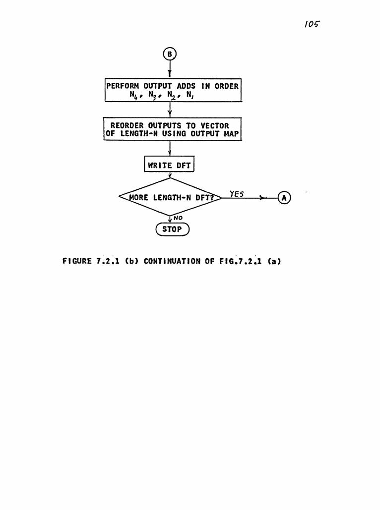
10 f

FIGURE 7.2.1 Cb) CONTINUATION OF FIG.7.2.1 (a)

106

Implemented on IBM370/155 In FORTRAN.

SECTION 7.3 : INDEX-MAP FOURIER ALGORITHM (IFA)

This program uses the non-1Inear Index mapping to

partition the tndtces Into groups as defined In (3.2.1).

The powers of w^ are partitioned according to the

tndex-map and Input adds are performed on these blocks of

data. After polnt-by-potnt multiply the output adds are

performed on the blocks. These are, then, merged according r

to the CRT map. Each element from a block Is, then, updated

from the values In other blocks and the resulting array Is

output according to the CRT map Into an output vector.

The flow of this program Is shown In Fig.7.3.1. The

Input to I FA program Is the data 1ength-N factors of N, the

number of factors, generators and the length of generators.

The last non-untty generator Is always (-1) mod.N-(N-l).

This allows the separation of the real and Imaginary

computation and further allows them to be performed In real

mode (see sect.6.4 eq.6.4.8). The program ts written for

two mutually prime factors and the available factors are 2,

3, 5 and 7. The maximum number of generators ts 3. The

unused generators when the number of generators Is less

than 3 and the unused factors when the number of factors Is

less than 2 are set to 1.

tog

FIGURE 7.3.1 Ca) FLOW CHART OF INDEX FOURIER ALGORITHM

FIGURE

los

.3.1 (b) CONTINUATION OF FIG. 7.3.1 (a)

no

CHAPTER 8 : COMPARI SONS,EVALUATIONS AND CONTRIBUTIONS

SECTION 8.1 : COMPARISONS AND EVALUATIONS

As shown, In sect. 5.9 (5.9.25) a major block of data

can be operated upon so that Its real and Imaginary parts

are computed seperately. Thus both real and Imaginary

calculations can be done tn real mode. This result extends

to other blocks tf these, too, can be made Into

multidimensional or are already multidimensional. Further,

the calculation of two different blocks does not require

any exchange of data, thus, It becomes possible to do most

of the computation of partial results (before final adds)

In parallel and in real mode. This Is a useful property for

hardware Implementation. In comparison to this. It is not

easily possible to do both the parallel processing and

seperatlon of real and Imaginary computation In other

algorithms like NFA and PFA. For Instance, In NFA, the

seperatlon of real and Imaginary parts would entail

calculation of even and odd parts of Input data . These

would, then, have to be streamed through seperate

algorithms similar to NFA, and therby doubltng the hardware

or the software.

Turntng to the comparisons of the arithmetic

computation required for these algorithms (Table 8.1.1), we

find that for all lengths the number of multiplies are the

same for both NFA and IFA, but less than that for PFA. The

reduction on the multiply count Is between 112 to 352.

Ill

However, the number of adds has Increased. The PFA has

between 132 to 392 fewer adds as compared to I FA. Same Is

true for comparison between NFA and I FA. We, also, note

that the number of adds for IFA tends to Increase less

rapidly than NFA after DFT length 455.

In comparing the timings (Tables 8.1.2 & 8.1.3), we

note that NFA requires bttween 192 to 352 more execution

time and this seems to tally with the requirement of more

adds for NFA and the larger amount of Indexing required.

The same Is true for the timings between IFA and NFA. Thus,

the number of adds and the amount of overhead make a

significant difference on the execution time.

Another Interesting aspect tn NFA Is that, when a

factor like 6 Is available as 6 as well as 3*2, the

execution time with use of factor 6 results tn a shorter

execution time than the factors 3*2. For Instance tn

210-7*6*5

Execution time for 7*6*5 * 0.1035 sec.

Execution time for 7*5*3*2-0.1131 sec.

Also, when ordering the factors 7*6*5 It Is better to

give precedence tn execution to factor with lower multiply

per point value. E.g.

N*6 ---> ^-1 mult./pt. , N-5 —•> ^_-l,2 mult./pt.

Execution time for 7*6*5 - 0,1035 sec, .

Execution time for 7*5*6 - 0.0991 sec

HZ

TRANS.

LENGTH

FACTORS PFA NFA IFA

MULT ADD MULT ADD MULT ADD

33 3,11 96 391 62 396 62 430

65 5,13 155 744 125 793 125 1071

66 2,3,11 164 892 125 804 125 1338

130 2,5,13 330 2424 251 2576 251 2989

195 3,5,13 625 3870 377 4059 377 4994

231 3,7,11 838 4145 566 4377 566 6090

273 3,7,13 914 5899 566 6459 566 6793

455 5,7,13 1675 10,538 1133 13,373 1133 13,138

715 5,13,11 3115 19,457 1645 26,179 2645 24,350

1001 7,13,11 4504 29,046 3968 40,770 3968 36,965

TABLE 8.1.X» MULTIPLY & ADD COUNTS FOR PFA,NFA AND I FA

113

TRAMS.

LENGTH

NESTED PFA t

CHANGE

60 0.026 0,017 35

210 0.099 0.08 19

315 0.173 0.111 31

504 0.236 0.168 28

840 0.466 0,344 26

1260 0.822 0,54 34

TABLE 8.1.2. TIMINGS IN SEC. FOR NFA & PFA

TRANS. IFA NFA *

LENGTH CHANGE

35 0.0158 0.0137 13

21 0.0118 0.00788 33

15 0.0083 0,0056 32

14 0.0071 0.0053 25

7 0.00212 0.00225 - 6

6 0.0034 0.0023 32

TABLE 8.1.3. TIMINGS IN SEC. FOR IFA & PFA

The cause of this reduction In timing Is due to the

reduction In the rate with which the data array Increases

In Its size during the Input add operation and the Increase

In the rate with which the output array decreases In tls

size during the output add operation* .

Evidently, on a machine, with timings for multiply and

add of the same order, PFA has the advantage of lower over

all arithmetic computation count. However, In an

environment where addition Is faster than multiplication

( say by a factor of 5 or more) IFA has certatn advantages

over PFA or NFA viz:

(a) partitioning of data Into Independent blocks.

(b) seperatlon of real and Imaginary parts of the

partial results.

In conclusion, with Implementation on appropriate

hardware (or software) the IFA algorithm offers the

advantage of parallel processing on parttttoned data In

real mode.

SECTION 8.2 : CONTRIBUTION OF THIS RESEARCH

In thts research, a fairly delatled analysis of

conditions for multidimensional mapping has been performed. .

Two different kinds of mappings viz., multidimensional

linear mapptng and multidimensional nonltnear tndex mapping

have been discussed In detail. A new representation of

nonltnear Index map has been developed. Application of each

ns

map to Discrete Fourier Transform has been shown*

Various methods of Implementing cyclic convolution

have been presented* Wtnograd has proposed a new

application of Chinese Remainder Theorm to polynomials for

reduction In the number of multiplies for convolution* This

has been presented, along with the use of multidimensional

map to convert the long length convolution to

multidimensional convolution, with shorter dimensions* An

Illustration of Wtnograd approach has been presented for

length-6 convolution.

An approach, suggested by Rader and Wtnograd to

convert short length DFT to convolution, has been utilised

to compute optimal DFT algorithms* This approach, along

with, multidimensional linear Index mapping have been used

to Implement a Nested Algorithm for DFT* The method of

converting short length DFT to convolution has been V

generalised by use of multidimensional non-1Inear map Index

map* A particular map, which allows seperatlon of

computation of real and Imaginary parts has been presented*

A program using the non-1tnear Index mapping has been

Implemented* .

The amount of computation required for the three

algorithms (PFA,NFA and !FA) has been compared for the

number of multiplies and adds and for timing required to

compute the DFT. A brief description of advantages and

disadvantages has been given and possible future

Improvements have been suggested*

REFERENCES

H6

<1> D.P.Kolba and T.W.Parks, " A Prime Factor FFT Algorithm Using High Speed Convolution",IEEE on Acoustics,Speech and Signal Processing, Vol• ASSP-25, No,4, August 1977.

<2> C.S.Burrus,"Index Mapping for Multidimensional Formulation of OFT and Convolution",IEEE Trans, on Acoustics,Speech and Signal Processing, Vol.ASSP-25,pp.259-242,dune 1977,

<3> !.J.Good,"The Interaction algorithm and practical Fourier series",J.Royal Statst.Soc,,ser B,Vol,20, pp361-372,1958; Addendum Vol,22,pp,372-375,1960.

<4> 0.Ore,"Number Theory and Its HIstory",McGrowhll1, New York,1948,

<5> R.C.Agarwal and d.W.Cooley,"New Algorithms for Digital Convolution",IEEE Acoustics,Speech and Signal Processing",Vol.ASSP-25,NO-5,Oct,1977,

<6> I.N.Herstetn,Topics In Algebra,2nd ed«, d.Utley & Sons,New York.

<7> J.W.Cooley and d,W.Tukey,"An Algortlthm for the machine calculation of Complex Fourier Series", Math. Comput.,Vol.19,pp-297-301,April 1965,

<8> S.Wtnograd,"0n computing The Discrete Fourier Transform."Proc.Nat.Acad.ScI,,U.S.A.,Vol,73,No,4, PP1005-1006,April 1976.

<9> C.Rader."Discrete Fourier Transform when the Number of Data Samples Is Prtme,",Proc,IEEE, Vol. 56,p.107-1108,dune 1968.

<10> I.N.Herstetn,Theorm 2,14,1 pp.l09,Toptcs tn Algebra,2nd ed.,Wt1ey & Sons,New York,1975,

<11> D.Shanks,"Solved and Unsolved Problems tn Number Theory, Spartan Books,New York,1962,

<12> R.C.Agarwal and C.S.Burrus,"Fast Convolution using Fermat Number Transforms with application to Digital Filtering",IEEE Trans.Acoustics,Speech and Signal Proc., Vol.ASSP-22,pp.87-97,April 74,

<13> ——,"Fast One-Dtmenstonal Digital Convolution by Multidimensional Techniques",IEEE Trans,Acoustics, Speech and Signal Proc,,Vol«ASSP-22,No.1,Feb,1974,

<14> S. WInograd#"Some Bilinear Forms whose Multiplicative Complexity Depends on the Field of Constants'1# 1 *B.M. Watson Research Center# Yorktown Heights# M.Y. 10598,

<15> J.0.Laderman#"A non-comutatIve algorithm for multiplication of 3x3.matrices using 23 . multlplles",Bull«Amer,Math,Soc.Vol,82#No,l#Jan 76,

<16> R.C.SIng1eton#"An Algorithm for Computing the Mixed Radix Fast Fourier Transform"#IEEE Trans, Audio Elecroacoust*#Vo1*AU-17#pp.93-103#June 1969,

<17> Quarterly Rep,l#EffIclent Techniques for Signal Processing# Baliastlc Missile Center# Control 9 DSAG 60-77-C-0091,

<18> Quarterly Rep.2#£fftctent Techniques for Signal Processing# Baliastlc Missile Center# Control # DSAG 60-77-C-0091.

<19> Renewal Res* Proposal# Efficient Techniques for Signal Processing# Baliastlc Mtsstle Center# Control 9 DSAG 60-77-C-0091,

<20> R. Bernstein,"Schnelle Faltung Mit Der Rader* Transformation ,(#D!p1omarbelt#Institut Fur Nachrtchtentechnlk# Unlversltat Erlangen-Nurnberg, dull 1974.

<21> W.M.Gentleman and G,Sande#"Fast Fourier Transform for fun and profit"# 1966 Fall Joint Computer Conf.#AFPIS Proc.#Voî-29,Washington,D.C. Spartan#1966#pp*563*578.

APPENDIX A

/M

LEMMA : If N ts an odd prtme then for Nf2*. M+l and k, M

Integers and k>2 the units ~HN can be written as a direct

product of two subgroups, one of which ts of order 2,

"Uw • , - zx ® Gp

where Gp Is a group of order Pj(N*2P+l).

PROOF : Since N ts an odd prime 0(N)»N-1 ts even and can

be written as

0CN)-N-1»2P

where P ts an Integer and because of the restriction on N Y

we have (2/P)*l. Let P* TT P; , where P; are odd primes.

Then/ by Cauchy's Theorm for abelian groups and Sylow's

Theorm for the abelian groups <X0/Ch.2/pp6X-62>/ there

exist Sylow subgroups of order 2 and of orders P{* / 1*1/

2/...r# such thatTlN ts Isomorphic to the direct product

of these Sylow subgroups.

11^ * ^2.02^ 0Zp%® *•••• IPy * ® Gp

where Gp ts of order P. V v+1 I If P»2 for some r>l then since 2 | 2P/ but

2y+2 )(zp then, by Sylow's Theorm one and only one cyclic */+/

subgroup exists and this ts of order 2 . Since ts

of order 2P*2T+I / Tlv cannot be expressed tsomorphlcal 1y

by a direct product of two cyclic subgroups. Y

In the case when N*P / P an odd prime/ P*2R+X/.

Pj^* +l/such that k>2/ then

A-2

and stnce 2 j (P-1) and £j[ (P-1), we have "UN ■ Ip_,® Zpt-i « Zx ® GR<£>ZP»-I «

v When N*2P, where P« 7T p. , p. distinct odd prime

powers and such that where r»l P*!*^* *1, k>2, then using

the fundamental theorm for finite abelian groups <10,ppl09>

UN can be written as a direct product of cyclic groups one

of which Is of order 2.

Y Finally, when N*2 , r>2 then

u* « za <g> z2^ .

8-1

APPENDIX B

B*1 : ALGORITHMS FOR OPTIMAL CONVOLUTION

This appendix will give the matrices A, B and C for

convolution to Implement the algorithm :

Y»CM

where M« AH 0 BX

The lengths considered here are those used for (FA

program.

CONVOLUTION LENGTH 2 :

aCO) -£<h(0)*ha>>

a(l) -£(h(0)-h(I)>

b(0) - xCO) ♦ x(l)

b(l) - x(0) - x(l)

2 multiplies , 4 adds .

CONVOLUTION LENGTH 3 :

a(0) -l(h(0)+h(l)+h(2))

a(l) - h(0) - h(2)

a(2) « h(l) - h(2)

aC3) -(ad) ♦ ad))/*

b(0) - x(0)*x(l)+x(3)

b(l) * x(0)-*x(2)

b(2) - x(l)-x(2)

b(3) * bU> ♦ b(2>

4 mult.,11 adds. .

yCO)* mCO) «■ m(l)

y(l)* m(0) - mCl)

y(0) * m(0) ♦ (m(l)-m(3))

y(l) - m(0) - (md)-m(3))

- (m(2)~m(3))

y(2) » m(0) ♦ (m(2)-m(3))

8-2

CONVOLUTION LENGTH 4 î

a(0) - 1/^ ( h(O) ♦ hCl) )

aCl) * l/4 C h(0) ♦ h(2) )

aC2) » l/z ( h(0> - h(2) )

a(3) - l/2 ( h(O) - h<2> )

a(4) - 1 j2 C h(O) - h(2) )

b(O) • ( x(O) ♦ x(2) ) ♦

bd) - ( xCO) ♦ x(2) ) -

b(2) - ( x(O) - x(2) ) ♦

b(3) - ( x(O) - x(2) )

b(4) « ( x(l) - x(3) )

y(O) - ( m(O) ♦ mCl) ) ♦

y(l) * ( m(O) - m(l) ) ♦

y<2) • ( m(O) ♦ mCl) ) -

y(4) » ( m(O) - rod) ) -

5 mult

♦ ( hd) ♦ h(3) )

- ( hd) ♦ h(3) )

- ( hd) - h(3) )

♦ ( hd) - h(3) )

( xd) 4 x(3) )

( xd) 4 X(3) )

( xd) - x(3) )

( m(2) - m(4) )

C m(2) - m(3) )

( m(2) - ro(4) )

C m(2) - m(3) )

• # 15 adds.

fi-3

B 2 : OFT ALGORITHMS FOR NESTED FOURIER ALGORITHM

Here the short length OFT algorithms are given for

1ength*2 to 9 along with multiply and add counts for real

data« The algorithms given here are similar to those given

In <1>. However the number of multiplies ts slightly higher

to make the algorithms suitable for use In NFA.

TRANSFORM LENGTH 2 $

aCD-l.O

a(2)«1.0

b(l)*x(0)*x(l)

b(2)«x(0)-x(l)

0 mult. , 2 w^-mult., 2 adds TRANSFORM LENGTH 3 :

a(l)*1.0 cl»mCl)-mC2)

a(2)-0.5 XC0)«mU>+m(2>*m<2)

a(3)-j0.8660254 X(1)«cl-m(3)

b(l)-x(0) x(2)-cl+m(3)

b(2)-x(l)+x(2)

b(3)«x(l)-x(2)

2 multiplies, 1 w°-multIply.,12 adds

X(0)*m(l)

X(l)«m(2)

9-k

TRANSFORM LENGTH 4 s

a(l)-1.0 X(0)*m(l)*m(3)

a(2)-1.0 X(l)*m(2)«-fn(4)

a(3)-1.0 X(2)*m(l)-m(3)

a(4)«jl,0 X(3)»m(2)-m(4)

b(l)«x(0)+x(2)

b(2)*x(0)-x(2)

b(3)»x(l)+x(3)

b(4)*x(l)-x(3)

0 multiplies, 4 vr^-mul tlpty , 12 adds

TRANSFORM LENGTH S :

a(l)«1.0 c0*m(2)+m(2)

a(2)-0.25 cl*m(l)-m(2)

a(3)-0.5509017 XC0)«c0^c0*m(l)

a(4)*J0.363271 c2»cl+m(4)

a(5)-jl.538842 c3*m(6)-m(4)

a(6)-j0.951057 X(l)*c2-c3

b(l)-x(0) X<4)«c2*c3

b(2)«(x(l)+x(4))*(x(2)+x(3)> c2*cl-m(4)

b(3)*(x(l)+x(4))-(x(2)*x(3)) c3*m(5)-m(6)

b(4)»x(2)-x(3) XC2)»c2-c3

b(5)*x(lJ-x(4) X(3)*c2+c3

b(6)»(x(l)-x(4))+(x(2)-x(3))

5 mult,,. 1 t/-mu1tlp1y, 31 adds.

Q-S

TRANSFORM LENGTH 6 :

a(l)-1.0 cl*m(l)-m(3)

a(2)-0.5 c2-m(2)-m(4)

a(3)«0.5 X(0)*m(l)+m(3)+m(3)

a(4)«0*5 X(I)*c2-m(6)

a(5)-j0.8660254 X(2)*cl+m<5)

a(6)-J0.8660254 X(3)»m(2)*m(4)+m(4)

b(l)-xC0>*x<3> X(4)*cl-m(5)

b(2)-x(0)-x(3)

b(3)*(x(4)+x(2))-(x(l)*x(5))

b(4)«(x(4)+x(2))-(x(l)+x(5))

b(5)-Cx(4)-x(2>)4(x(l)-x(5))

b(6)*(x(4)-x(2))-(x(4)~x(5))

X(5)-c2+m(6)

4 multiplies # 2 w^-multIpHes # 30 adds*

TRANSFORM LENGTH 7 s

a(l)«1.0 c0-m(2)+m(2)+m(2)

a(2)-0,16666667 cl-m(l)-m(2)

a(3)-0.790156 c2-cl+m(3)+m(4)

a(4)-0.055854 c3*cl-m(3)-m(5)

a(5)«0.734302 c4»cl-m(4)♦m(5)

a(6)-j0.440959 c5»m(6)♦m(7)-m(8)

a(7)-J0.340873 c6»m( 6)-mC 7)-m(8)

a(8)-J0.533969 c7-m(6)+m(7)+m(8)

a(9)-j0.874842

sl-x(l)+x(6) y(0)*m(l)^c0^c0

s2-x(l)-x(6) y(l)»c2-c5

s3-x(2)+x(5) y(2)»c3-c6

s4«x(2)-x(5) y(3)*c4+c7

s5«x(3)*x(4) y(4)-c4-c7

s6«x(3)-x(4) y(5)*c3*c6

bU)-x(O) y(6)*c2*c5

b(2)«sl+s3+s5

b(3)*sl-s5

b(4)»s5-s3

b(5)*s3-sl

b(6)«s2*s4-s6

b(7)-s2+s6

b(8)*-s4-sfi

b(9)-s4-s2

8 mult.,1 w° mu1t.# 55 adds*

TRANSFORM LENGTH 8 :

8-7

a(l)-1.0 cl«m(4)+m(5)

a(2)-1.0 c2*m(4)-m(5)

a(3)»1.0 c3«,m(7)<»>in(8)

a(4)«1.0 c4»m(7)-in(8)

a(5)-0.707107 X(0)-ml

a($)-jl.O X(I)*cl*c3

a(7)*jl.O X(2)»m(3)>m(6)

a(8)-j0.707107 XC3)«c2-c4

sl«x(0)+x(4) X(4)*m2

s2«x(2)+x(6) X(5)*c2+c4

s3«xU)*x<5) X(6)«m(3)-m(6)

s4-x(l)-x(5)

s5«xC3)*x(7>

s6*x(3)-x(7)

s7»sl*s2

s8*s3*s5

b(l)-s7+s8

b(2)«s7-s8

b(3)-sl-s2

b(4)»x(0)-x(4)

b(5)-s4-s6

b(6)-s3-s5

b(7)-x(2)-x(4>

X(7)*cl-c3

b(8)»s4+s6

2 mult., 6 *t° mult., 36 adds.

TRANSFORM LENGTH 9

3-8

a(l)-1.0 cl»m(l)-m(2)

a(2)»0.5 c2»m(5J-m(6)

a(3)-0.5 c3*m(4)+m(6)

a(4)-0.197465 c4«m(4)+m(5)

a(5)-0.568579 c5»cl*c2-c3

a(6)«0.371114 c6»cl*c3*c4

a(7)-j0.542532 c7*»cl-c2-c4

a(8)-j0.100256 c8»m(7)-m(9)

a(9)-j0.442276 c9»m(8)-m(9)

a(10)»j0.8660254 cl0»m(7)-m(8)

a(ll)-jO.8660254 cll-c8+c9+m(10)

sl-x(l)+x<8) cl2»c8+cl0-m(10)

s2»x(l)-x(8) cl3-cl0-c9+m(10)

s3-x(2)+x(7) ccl3«m(l)+m(2)+m(2)

s4»x(2)-x(7) cl4«ccl3-m(3)

s5«x(4)*x(5)

s6«x(4)-x(5) X(0)-ccl3+m(37<nn(3)

b(l)-x<0) X(l)-c5-cll

b(2)-x(3)+x(6) X(2)*c6-cl2

b(3)«sl*s3*s5 X(3)«cl4-m(ll)

b(4)*s5-sl X(4)*c7-cl3

b(5)-sl-s3 X(5)«c7*cl3

b(6)*s5-s3 b(9)*-s4-s6 X(6)«cl4+m(ll)

b(7)»s2-s6 b(10)«x(3)-x(6) X(7)»c6+cl2

b(8)«s2+s4 b(ll)»s2-s4+s6 X(8)*c5*cll

10 mult*, 1 w° mult ** 74 adds