Applications of Deep Neural Networks to Protein Structure Prediction _______________________________________ A Dissertation presented to the Faculty of the Graduate School at the University of Missouri-Columbia _______________________________________________________ In Partial Fulfillment of the Requirements for the Degree Doctor of Philosophy _____________________________________________________ by CHAO FANG Professor Yi Shang, Dissertation Advisor Professor Dong Xu, Dissertation Co-advisor

Welcome message from author
This document is posted to help you gain knowledge. Please leave a comment to let me know what you think about it! Share it to your friends and learn new things together.
Transcript

Applications of Deep Neural Networks to Protein Structure Prediction
_______________________________________
A Dissertation
presented to
the Faculty of the Graduate School
at the University of Missouri-Columbia
_______________________________________________________
In Partial Fulfillment
of the Requirements for the Degree
Doctor of Philosophy
_____________________________________________________
by
CHAO FANG
Professor Yi Shang, Dissertation Advisor
Professor Dong Xu, Dissertation Co-advisor
COPYRIGHTS
Chapter 3 © Wiley Periodicals, Inc.
Chapter 4 © IEEE
Chapter 5 © IEEE
All other materials © Chao Fang

The undersigned, appointed by the Dean of the Graduate School, have examined the dissertation entitled
Applications of Deep Neural Networks to Protein Structure Prediction
presented by Chao Fang,
a candidate for the degree of Doctor of Philosophy
and hereby certify that, in their opinion, it is worthy of acceptance.
Dr. Yi Shang
Dr. Dong Xu
Dr. Jianlin Cheng
Dr. Tim Trull
DEDICATIONS
To my father Weimin Fang and my mother Li Li.

ii
ACKNOWLEDGEMENTS
I would like to take the opportunity to thank the following people who have supported
me through my PhD experience. Without the support of them, this dissertation would not
have been possible.
First, I would like to thank my advisor, Professor Yi Shang, for his eight years of patient
teaching and guidance. I have been learning knowledge and perform research with him
since I first came to Mizzou as a junior student in the “2+2” cooperative Computer Science
undergraduate program. Working with him has become a great unforgettable experience in
my life. He gradually teaches me hands-on experience on how to perform research, carry
out experiments, teach, write scientific articles and give technical presentations step by
step. He not only teaches me the knowledge of Artificial Intelligence and machine learning,
but he also teaches me the scientific attitude of being a researcher, one should always be
humble to take opinions from other researchers and always chasing the excellence in
research. I thank his never-ending patient guidance and trust, warm-heart help, which are
essential for the success of my PhD research. Professor Shang not only gives me
suggestions on my research study, but also on my life and career path. His critical scientific
research spirit will always inspire me.
I wish to thank my co-advisor, Professor Dong Xu, for his tireless help with answering
my questions on Bioinformatics. He leads me walking into the fascinating research world
of Bioinformatics to explore the beauty of life sciences. I once got lost in the bioinformatics
research, it is Professor Xu led me step out of the maze. It is his confidence, optimism and

iii
his insightful research suggestions inspire me to solve hard problems when facing the
research difficulties.
I wish to thank my committee member, Professor Jianlin Cheng, for giving me
constructive suggestions to my dissertation work. I took many of his interesting courses in
the past few semesters, such as supervised learning, data mining, machine learning for
Bioinformatics and computational optimization methods. Many of his class materials and
projects are helpful to my PhD research. I also wish to thank my committee member,
Professor Tim Trull, who gives me constructive advice for this dissertation.
Many thanks to my coworkers Zhaoyu Li, Peng Sun, Guang Chen, Duolin Wang, Junlin
Wang, Wenbo Wang, Yang Liu, and Sean Lander for helping me learning protein structure
prediction, helpful discussion, useful ideas and friendship. It is a memorable experience
that we went to attend the ICTAI-2017 conference together in Boston to present our
research work.
Last but not least, I wish to thank my father Weimin Fang and my mother Li Li. Without
their support and foresight, I would not be able to study abroad in America. Without their
encouragement and love, I would not have been this far. I wish to dedicate this dissertation
to my parents.
This work was partially supported by the National Institutes of Health grant R01-
GM100701. The high-performance computing infrastructure was partially supported by
the National Science Foundation under grant number CNS-1429294.

iv
TABLEOFCONTENTS
COPYRIGHTS ................................................................................................................... 2
DEDICATIONS .................................................................................................................. 4
TABLE OF CONTENTS ..................................................................................................... iv
LIST OF FIGURES....................................................................................................... x
Chapter 1 INTRODUCTION .............................................................................................. 1
1.1 Protein Sequence, Structure and Function ................................................................. 1
1.2 Protein Secondary Structure Prediction ..................................................................... 2
1.3 Protein Backbone Torsion Angle Prediction ............................................................... 4
1.4 Protein Beta Turn Prediction ..................................................................................... 6
1.5 Protein Gamma Turn Prediction ................................................................................ 7
1.6 Contributions ............................................................................................................. 8
1.7 Outline of the Dissertation ........................................................................................ 9
Chapter 2 RELATED WORK AND BACKGROUND............................................................ 11
2.1 Protein Secondary Structure Prediction ................................................................... 11
2.2 Protein Backbone Torsion Angle Prediction ............................................................. 14
2.3 Protein Beta-turn Prediction .................................................................................... 17
2.4 Protein Gamma-turn Prediction ............................................................................... 19
2.5 Deep Neural Network .............................................................................................. 20
2.6 Convolutional Neural Network ................................................................................ 21
2.7 Residual Neural Network (ResNet) .......................................................................... 22

v
2.8 ReLU, Batch Normalization and Fully Connected Layer ............................................ 23
2.9 Dense Network ........................................................................................................ 25
2.10 Capsule Network...................................................................................................... 25
Chapter 3 NEW DEEP INCEPTION-INSIDE-INCEPTION NETWORKS FOR PROTEIN
SECONDARY STRUCTURE PREDICTION .......................................................................... 27
3.1 Problem Formulation ............................................................................................... 27
3.2 New deep inception networks for protein secondary structure prediction ............. 29
3.3 New deep inception-inside-inception networks for protein secondary structure
prediction (Deep3I) .............................................................................................................. 31
3.4 Experimental Results ............................................................................................... 33
3.4.1 PSI-BLAST vs. DELTA-BLAST ................................................................................... 35
3.4.2 Deep3I vs. the Best Existing Methods ................................................................... 36
3.4.3 Effects of Hyper-Parameters of Deep3I ................................................................. 38
3.4.4 Results Using Most Recently Released PDB Files ................................................... 39
Chapter 4 A NEW DEEP NEIGHBOR RESIDUAL NETWORK FOR PROTEIN SECONDARY
STRUCTURE PREDICTION .............................................................................................. 41
4.1 DeepNRN – Deep Neighbor-Residual Network ........................................................ 41
4.1.1 DeepNRN Architecture ......................................................................................... 41
4.1.2 Batch Normalization and Dropout ........................................................................ 44
4.1.3 Input Features ...................................................................................................... 44
4.1.4 Struct2Struct Network and Iterative Fine-tuning .................................................. 45
4.2 Experimental Results ............................................................................................... 47

vi
4.2.1 Performance Comparison of DeepNRN with Other State-of-the-art Tools Based on
the CB513 Data set ........................................................................................................... 48
4.2.2 Performance Comparison of DeepNRN with Other State-of-the-art Tools Based on
Four Widely Used Data sets .............................................................................................. 49
4.2.3 Effect of Convolution Window Size in Struct2Struct Network and Iterative
Refinement ....................................................................................................................... 50
4.2.4 Exploration of other Network Configurations of DeepNRN ................................... 53
Chapter 5 PROTEIN BACKBONE TORSION ANGLES PREDICTION USING DEEP RESIDUAL
INCEPTION NETWORKS ................................................................................................. 55
5.1 Problem formulation ............................................................................................... 55
5.2 New Deep Residual Inception Networks (DeepRIN) for Torsion Angle Prediction ... 58
5.3 Experimental Results ............................................................................................... 62
Chapter 6 PROTEIN BETA TURN PREDICTION USING DEEP DENSE INCETPION
NETWORKS ................................................................................................................... 72
6.1 Methods and Materials............................................................................................ 72
6.1.1 Preliminaries and Problem Formulation................................................................ 72
6.1.2 New Deep Dense Inception Networks for Protein Beta-turn Prediction (DeepDIN)75
6.1.3 Apply Transfer Learning and Balanced Learning to DeepDIN to Handle Imbalanced
Dataset 78
6.1.4 Benchmark datasets ............................................................................................. 80
6.2 Results and Discussion ............................................................................................. 81
6.2.1 How Feature Affects the DeepDIN Performance ................................................... 81

vii
6.2.2 Residue-Level and Turn-Level Two-Class Prediction on BT426 .............................. 83
6.2.3 Turn-level Nine-Class Prediction on BT6376 .......................................................... 84
Chapter 7 PROTEIN GAMMA TURN PREDICTION USING DEEP DENSE INCETPION
NETWORKS ................................................................................................................... 86
7.1 Materials and Methods............................................................................................ 86
7.1.1 Problem formulation ............................................................................................ 86
7.1.2 Model Design ....................................................................................................... 88
7.1.3 Model Training ..................................................................................................... 92
7.1.4 Experiment Dataset .............................................................................................. 92
7.2 Experimental Results ............................................................................................... 94
7.3 Conclusion and Discussion ..................................................................................... 105
Chapter 8 SUMMARY .................................................................................................. 107
REFERENCE.................................................................................................................. 114
VITA ............................................................................................................................ 132

viii
LIST OF TABLES
TABLE 1.1NINE TYPES OF BETA-TURNS AND THEIR DIHEDRAL ANGLES OF CENTRAL RESIDUES IN DEGREES
(THE LOCATIONS OF PHI1, PSI1, PHI2 AND PSI2 ARE ALSO ILLUSTRATED IN FIGURE 1) ......................... 6
TABLE 3.1 COMPARISON OF THE PROFILE GENERATION EXECUTION TIME AND DEEP3I Q3 ACCURACY
USING PSI-BLAST AND DELTA-BLAST .............................................................................................. 36
TABLE 3.2 Q8 ACCURACY (%) COMPARISON BETWEEN MUFOLD-SS AND EXISTING STATE-OF-THE-ART
METHODS USING THE SAME SEQUENCE AND PROFILE OF BENCHMARK CB513. ............................. 37
TABLE 3.3 Q3 ACCURACY (%) COMPARISON BETWEEN MUFOLD-SS AND OTHER STATE-OF-THE-ART
METHODS ON CASP DATASETS. ..................................................................................................... 37
TABLE 3.4 Q8 ACCURACY (%) COMPARISON BETWEEN DEEP3I AND OTHER STATE-OF-THE-ART METHODS
ON CASP DATASETS. ...................................................................................................................... 37
TABLE 3.5 Q3 ACCURACY (%) COMPARISON BETWEEN MUFOLD-SS WITH DIFFERENT NUMBER OF BLOCKS
AND DEEP INCEPTION NETWORKS WITH DIFFERENT NUMBER OF MODULES.................................. 38
TABLE 3.6 Q8 ACCURACY (%) COMPARISON BETWEEN DEEP3I WITH DIFFERENT NUMBER OF BLOCKS AND
DEEP INCEPTION NETWORKS WITH DIFFERENT NUMBER OF MODULES. ........................................ 39
TABLE 3.7 Q3 (%) AND Q8 (%) COMPARED WITH MUFOLD-SS AND OTHER STATE-OF-THE-ART TOOLS
USING RECENTLY PDB. ................................................................................................................... 40
TABLE 4.1 PERFORMANCE COMPARISON OF DEEPNRN, SSPRO, AND PSIPRED ON Q3 AND Q8 ACCURACY
ON THE CB513 DATA SET. .............................................................................................................. 48
TABLE 4.2 Q3 (%) ACCURACY RESULTS OF VARIOUS PREDICTION METHODS ON FOUR DATA SETS. .......... 49
TABLE 4.3 Q8 (%) ACCURACY RESULTS OF VARIOUS PREDICTION METHODS ON FOUR DATA SETS. .......... 50
TABLE 4.4 OTHER NETWORK CONFIGURATION OF DEEPNRN AND PERFORMANCE .................................. 53
TABLE 5.1 COMPARISON OF MEAN ABSOLUTE ERRORS (MAE) OF PSI-PHI ANGLE PREDICTION BETWEEN
DEEPRIN AND BEST EXISTING PREDICTORS USING THE TEST SETS FROM (LI ET AL., 2017) ............... 65
ix
TABLE 5.2 COMPARISON OF MEAN ABSOLUTE ERRORS (MAE) AND PEARSON CORRELATION COEFFICIENT
(PCC) OF PSI-PHI ANGLE PREDICTION BETWEEN DEEPRIN, SPIDER2 AND SPIDER3 USING THE CASP10,
11 AND 12 DATASETS. THE PCC IS WRITTEN IN PARENTHESES. BOLD-FONT NUMBERS IN EACH
COLUMN REPRESENT THE BEST RESULT ON A PARTICULAR DATASET. ............................................ 65
TABLE 5.3 COMPARISON OF MEAN ABSOLUTE ERRORS (MAE) AND PEARSON CORRELATION COEFFICIENT
(PCC) OF PSI-PHI ANGLE PREDICTION BETWEEN DEEPRIN AND SPIDER2 AND SPIDER3 USING THE
RECENTLY RELEASED PDB DATASET. THE PCC IS SHOWN IN PARENTHESES. .................................... 67
TABLE 5.4 COMPARISON OF MEAN ABSOLUTE ERRORS (MAE) OF PSI-PHI ANGLE PREDICTION BETWEEN
DEEPRIN AND SPIDER3 USING THE SAME TRAINING DATASET (SPIDER’S TRAINING SET) AND THE
SAME TEST DATASET. .................................................................................................................... 71
TABLE 6.1 DIFFERENT FEATURE COMBINATIONS WILL AFFECT PREDICTION PERFORMANCE .................... 82
TABLE 6.2 RESIDUE-LEVEL PREDICTION ON BT426 ................................................................................... 83
TABLE 6.3 TURN-LEVEL PREDICTION ON BT426 ....................................................................................... 83
TABLE 7.1 EFFECT OF WINDOW SIZE ON MCC PERFORMANCE................................................................. 95
TABLE 7.2 EFFECT OF DROPOUT ON MCC PERFORMANCE ....................................................................... 95
TABLE 7.3 EFFECT OF TRAINING SIZE ON TRAINING TIME AND MCC PERFORMANCE ............................... 95
TABLE 7.4 EFFECT OF DYNAMIC ROUTING ON MCC PERFORMANCE ........................................................ 95
TABLE 7.5 PERFORMANCE COMPARISON WITH PREVIOUS PREDICTORS USING GT320 BENCHMARK. ...... 98
TABLE 7.6 NON-TURN, INVERSE AND CLASSIC TURN PREDICTION RESULTS. ........................................... 100
TABLE 7.7 ABLATION TEST..................................................................................................................... 105

x
LIST OF FIGURES
FIGURE 1-1 AN ILLUSTRATION OF WHAT PSI-PHI ANGLES ARE ................................................................... 5
FIGURE 1-2 AN ILLUSTRATION OF WHAT A BETA-TURN IS. C, O, N, AND H, REPRESENT CARBON, OXYGEN,
NITROGEN AND HYDROGEN ATOMS, RESPECTIVELY. R REPRESENTS SIDE CHAIN. THE DASHED LINE
REPRESENTS THE HYDROGEN BOND. ............................................................................................... 7
FIGURE-1-3 AN ILLUSTRATION OF GAMMA-TURNS. RED CIRCLES REPRESENT OXYGEN; GREY CIRCLES
REPRESENT CARBON; AND BLUE CIRCLES REPRESENT NITROGEN. .................................................... 8
FIGURE 2-1 A RELU ACTIVATION FUNCTION PLOT. .................................................................................. 23
FIGURE 2-2 A FULLY CONNECTED NETWORK. .......................................................................................... 24
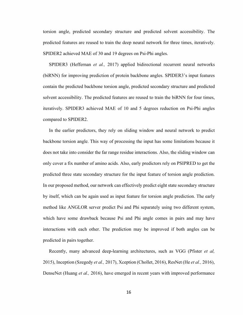
FIGURE 3-1 AN INCEPTION MODULE. THE RED SQUARE “CONV(1)” STANDS FOR CONVOLUTION
OPERATION USING WINDOW SIZE 1 AND THE NUMBER OF FILTERS IS 100. THE GREEN SQUARE
“CONV(3)” STANDS FOR CONVOLUTION OPERATION USING WINDOW SIZE 3 AND THE NUMBER OF
FILTERS IS 100. THE YELLOW SQUARE “CONCATENATE” STANDS FOR FEATURE CONCATENATION. . 30
FIGURE 3-2 A DEEP INCEPTION NETWORK CONSISTING OF THREE INCEPTION MODULES, FOLLOWED BY
ONE CONVOLUTION AND TWO FULLY-CONNECTED DENSE LAYERS. ............................................... 31
FIGURE 3-3 A DEEP INCEPTION-INSIDE-INCEPTION (DEEP3I) NETWORK THAT CONSISTS OF TWO DEEP3I
BLOCKS. EACH DEEP3I BLOCK IS A NESTED INCEPTION NETWORK SELF. THIS NETWORK WAS USED
TO GENERATE THE EXPERIMENTAL RESULTS REPORTED IN THIS PAPER. ......................................... 32
FIGURE 4-1 THE BASIC BUILDING BLOCK OF DEEPNRN, I.E., NEIGHBOUR-RESIDUAL UNIT. THE SQUARE
“CONV3” STANDS FOR CONVOLUTION OPERATION USING A WINDOW SIZE 3, WHILE THE SQUARE
“CONCATENATE” STANDS FOR FEATURE CONCATENATION. ........................................................... 42
FIGURE 4-2 NEIGHBOUR-RESIDUAL BLOCK HAS STACKS OF NEIGHBOR-RESIDUAL UNITS. ........................ 43
FIGURE 4-3 DEEP NEIGHBOR-RESIDUAL NETWORK (DEEPNRN) ARCHITECTURE. ...................................... 43
xi
FIGURE 4-4 (A) EFFECT ON Q8 OF ITERATIVE REFINEMENT BY APPLYING THE STRUCT2STRUCT NETWORK
REPEATEDLY. (B) LEFT TABLE SHOWS THE CONFUSION MATRIX OF THE PREDICTION RESULT OF
DEEPNRN, AND THE RIGHT TABLE SHOWS THE PREDICTION RESULT OF ADDING ONE STRUT2STRUCT
NETWORK LAYER OF WINDOW-SIZE 21. ......................................................................................... 52
FIGURE 4-5 (A) EFFECT ON Q3 OF ITERATIVE REFINEMENT BY REPEATEDLY APPLYING STRUCT2STRUCT
NETWORK. (B) LEFT TABLE SHOWS THE CONFUSION MATRIX OF THE PREDICTION RESULT OF
DEEPNRN, AND THE RIGHT TABLE SHOWS THE PREDICTION RESULT OF ADDING ONE
STRUCT2STRUCT NETWORK LAYER OF WINDOW-SIZE 21. .............................................................. 53
FIGURE 5-1 AN EXAMPLE OF THE PHYSICO-CHEMICAL FEATURE VECTOR OF A PROTEIN SEQUENCE. EACH
AMINO ACID IN THE PROTEIN SEQUENCE IS REPRESENTED AS A VECTOR OF 8 REAL NUMBERS
RANGING FROM -1 TO 1. THE FEATURE VECTORS OF THE FIRST 5 AMINO ACIDS ARE SHOWN. ....... 56
FIGURE 5-2 AN EXAMPLE OF THE PSI-BLAST PROFILE OF A PROTEIN SEQUENCE. EACH AMINO ACID IN THE
PROTEIN SEQUENCE IS REPRESENTED AS A VECTOR OF 21 REAL NUMBERS RANGING FROM 0 TO 1.
THE FEATURE VECTORS OF THE FIRST 5 AMINO ACIDS ARE SHOWN. THE THIRD THROUGH THE 19TH
COLUMNS ARE OMITTED. .............................................................................................................. 57
FIGURE 5-3 AN EXAMPLE OF THE HHBLITS PROFILE OF A PROTEIN SEQUENCE. EACH AMINO ACID IN THE
PROTEIN SEQUENCE IS REPRESENTED BY A VECTOR OF 31 REAL VALUES RANGING FROM 0 TO 1. THE
FEATURE VECTORS OF THE FIRST 5 AMINO ACIDS ARE SHOWN. ..................................................... 57
FIGURE 5-4 A RESIDUAL-INCEPTION MODULE OF DEEPRIN. THE GREEN RHOMBUS “CONV(1)” DENOTES A
CONVOLUTION OPERATION USING WINDOW SIZE 1 AND THE NUMBER OF FILTERS IS 100. THE
ORANGE SQUARE “CONV(3)” DENOTES A CONVOLUTION OPERATION USING WINDOW SIZE 3 AND
THE NUMBER OF FILERS IS 100. THE BLUE OVAL “CONCATENATE” DENOTES FEATURE
CONCATENATION. ......................................................................................................................... 59
FIGURE 5-5 ARCHITECTURE OF THE PROPOSED DEEP RESIDUAL INCEPTION NETWORK ARCHITECTURE
(DEEPRIN). ..................................................................................................................................... 60

xii
FIGURE 5-6 AVERAGE PSI-PHI ANGLES PREDICTION ERROR (MAES) FOR EACH OF THE EIGHT TYPES OF
SECONDARY STRUCTURE ON THE CASP12 DATASET BY DEEPRIN. ................................................... 68
FIGURE 5-7 PSI-PHI ANGLE PREDICTION RESULTS OF TWO PROTEINS IN CASP12, T0860 (TOP) AND T0861
(BOTTOM). PREDICTED ANGLE VALUE, TRUE ANGLE VALUE, AND ABSOLUTE ERROR ARE PLOTTED
FOR EACH AMINO ACID POSITION, WHICH IS LABELLED BY ITS TRUE SECONDARY STRUCTURE TYPE.
THE LOW BLUE BARS, WHICH DENOTE THE ERROR BETWEEN PREDICTED ANGLES AND TRUTH
ANGELS. ........................................................................................................................................ 70
FIGURE 6-1 (A) SHOWS THE OVERALL PROPOSED MODEL FOR BETA-TURN PREDICTION. (B) SHOWS THE
DETAILS OF A DENSE INCEPTION MODULE THAT CONSISTS OF FOUR INCEPTION MODULES, EACH OF
WHICH IS FULLY CONNECTED IN A FEED FORWARD FASHION. ........................................................ 78
FIGURE 7-1 (A) A DEEP INCEPTION CAPSULE NETWORK DESIGN. THE INPUT FEATURES ARE HHBLITS
PROFILE (17-BY-30 2D ARRAY) AND PREDICTED SHAPE STRING USING FRAG1D (17-BY-15 2D ARRAY).
EACH FEATURE IS CONVOLVED BY A CONVOLUTIONAL LAYER. BOTH CONVOLVED FEATURES THEN
GET CONCATENATED. AN INCEPTION BLOCK IS FOLLOWED TO EXTRACT LOW TO MEDIUM
FEATURES. A PRIMARY CAPSULE LAYER THEN EXTRACTS HIGHER LEVEL FEATURES. THE FINAL TURN
CAPSULE LAYER MAKES PREDICTIONS. (B) AN INCEPTION BLOCK. INSIDE THIS INCEPTION BLOCK:
RED SQUARE CONV(1) STANDS FOR CONVOLUTION OPERATION WITH KERNEL SIZE 1. GREEN
SQUARE CONV(3) STANDS FOR CONVOLUTION OPERATION WITH KERNEL SIZE 3. YELLOW SQUARE
STANDS FOR FEATURE MAP CONCATENATION. (C) ZOOM-IN BETWEEN PRIMARY CAPSULES AND
TURN CAPSULES. THE PRIMARY CAPSULE LAYER CONTAINS 32 CHANNELS OF CONVOLUTIONAL 8D
CAPSULES. THE FINAL LAYER TURN CAPSULE HAS TWO 16D CAPSULES TO REPRESENT TWO STATES
OF THE PREDICTED LABEL: GAMMA-TURN OR NON-GAMMA-TURN. THE COMPUTATION BETWEEN
THOSE TWO LAYERS IS DYNAMIC ROUTING. .................................................................................. 90

xiii
FIGURE 7-2 THE FITTING CURVE OF PRECISION (PERCENTAGE OF TRUE POSITIVE IN THE BIN) VERSUS THE
CAPSULE LENGTH. THE GREEN LINE IS THE FITTING CURVE AND THE BLUE LINE (Y=X^2) IS FOR
REFERENCE. ................................................................................................................................... 97
FIGURE 7-3 TRAINING LOSS AND VALIDATION LOSS CURVE OF DEEP INCEPTION CAPSULE NETWORK FOR
CLASSIC AND INVERSE GAMMA-TURN. .......................................................................................... 99
FIGURE 7-4 T-SNE PLOTS OF CAPSULE NETWORK FEATURES. (A) AND (B) ARE PLOTS OF THE INPUT
FEATURES AND THE CAPSULE FEATURES, RESPECTIVELY FOR TRAINING DATASET (3000 PROTEINS
WITH 1516 TURN SAMPLES). (C) AND (D) ARE PLOTS OF THE INPUT FEATURES AND THE CAPSULE
FEATURES, RESPECTIVELY FOR THE TEST DATASET (500 PROTEINS WITH 312 TURN SAMPLES). RED
DOTS REPRESENT NON-TURNS, GREEN DOTS REPRESENT INVERSE TURNS AND BLUE DOTS
REPRESENT CLASSIC TURNS. ........................................................................................................ 103
FIGURE 7-5 (A) CLASSIC TURN WEBLOGO; (B) INVERSE TURN WEBLOGO; AND (C) NON-TURN WEBLOGO
................................................................................................................................................... 104

xiv
APPLICATIONS OF DEEP NEURAL NETWORKS TO PROTEIN STRUCTURE
PREDICTION
Chao Fang
Professor Yi Shang, Dissertation Advisor
Professor Dong Xu, Dissertation Co-advisor
ABSTRACT
Protein secondary structure, backbone torsion angle and other secondary structure
features can provide useful information for protein 3D structure prediction and protein
functions. Deep learning offers a new opportunity to significantly improve prediction
accuracy. In this dissertation, several new deep neural network architectures are proposed
for protein secondary structure prediction: deep inception-inside-inception (Deep3I)
networks and deep neighbor residual (DeepNRN) networks for secondary structure
prediction; deep residual inception networks (DeepRIN) for backbone torsion angle
prediction; deep dense inception networks (DeepDIN) for beta turn prediction; deep
inception capsule networks (DeepICN) for gamma turn prediction. Every tool was then
implemented as a standalone tool integrated into MUFold package and freely available to
research community. A webserver called MUFold-SS-Angle is also developed for protein
property prediction.
The input feature to those deep neural networks is a carefully designed feature matrix
corresponding to the primary amino acid sequence of a protein, which consists of a rich set
of information derived from individual amino acid, as well as the context of the protein
sequence. Specifically, the feature matrix is a composition of physio-chemical properties
xv
of amino acids, PSI-BLAST profile, HHBlits profile and/or predicted shape string. The
deep architecture enables effective processing of local and global interactions between
amino acids in making accurate prediction. In extensive experiments on multiple datasets,
the proposed deep neural architectures outperformed the best existing methods and other
deep neural networks significantly: The proposed DeepNRN achieved highest Q8 75.33,
72.9, 70.8 on CASP 10, 11, 12 higher than previous state-of-the-art DeepCNF-SS with
71.8, 72.3, and 69.76. The proposed MUFold-SS (Deep3I) achieved highest Q8 76.47,
74.51, 72.1 on CASP 10, 11, 12. Compared to the recently released state-of-the-art tool,
SPIDER3, DeepRIN reduced the Psi angle prediction error by more than 5 degrees and the
Phi angle prediction error by more than 2 degrees on average. DeepDIN outperformed
significantly BetaTPred3 in both two-class and nine-class beta turn prediction on
benchmark BT426 and BT6376. DeepICN is the first application of using capsule network
to biological sequence analysis and outperformed all previous gamma-turn predictors on
benchmark GT320.
1
CHAPTER1 INTRODUCTION
1.1 ProteinSequence,StructureandFunction
Protein sequence, or called primary structure of protein, is a sequence of amino acid
residues, pair of which is connected by peptide bonds (Sanger and Thompson, 1953). Each
amino acid can be one of the twenty different amino acid residues.
Protein secondary structures can be alpha helix, beta sheet, and coil (Pauling and Corey,
1951). The secondary structure of a protein can provide constraints to the protein sequence.
Due to hydrophobic forces and side chain interactions between amino acids, protein
sequence will fold into stable tertiary structure (Dill, 1990). Two or more tertiary structures
will bind together to form the protein quaternary structure.
Previous research work has found that protein structures can determine the protein
function (Kendrew et al., 1960; Bjorkman and Parham, 1990). Proteins functions can be
enzymatic catalysis, transport and storage, coordinated motion, mechanical support,
immune protection, generation and transmission of nerve impulses, and control of growth
and differentiation (Laskowski et al., 2003). To understand better what protein functions
are, it is important to discovery the protein tertiary structure.
Currently, scientists applied physical methods to determine the protein tertiary structure
by using X-ray Crystallography (Bragg, 1975) and Nuclear Magnet Resonance (NMR)
spectroscopy (Wuthrich, 1986). So far, the number of discovered protein structure are
around 125,000 by the year of 2017 according to the statistics in the Protein Data Bank
(PDB) (Berman et al., 1999). However, there are still millions of protein sequences, whose

2
structure remains unknown and it is time-consuming and labor-intensive to use the
abovementioned physical methods to discover the protein tertiary structure.
Early researchers found that the protein sequence can dictate a tertiary structure (Sanger
and Thompson, 1953; Anfinsen, 1973), which has founded a heated research area:
predicting a protein tertiary structure from its sequence in computational or structural
biology. On one hand, predicting protein tertiary structure from its sequence can save time
and labor; on the other hand, it provides imperative and useful information to medical
sciences such as drug design (Jacobson and Sali, 2004).
1.2 ProteinSecondaryStructurePrediction
The way in which protein secondary structure elements are permutated and packed
(Murzin et al., 1995; Dai and Zhou, 2011) has a large effect on how the protein folds. If
the protein secondary structure can be predicted accurately, it can provide useful
constraints for 3D protein structure prediction. The protein secondary structure can also
help identify protein function domains and may guide the rational design of site-specific
mutation experiments (Drozdetskiy et al., 2015). Thus, accurate protein secondary
structure prediction would have a major impact on the protein 3D structure prediction
(Zhou and Troyanskaya, 2014; Fischer and Eisenberg, 1996; Skolnick et al., 2004; Rohl
et al., 2004; Wu et al., 2007), solvent accessibility prediction (Fauchere et al., 1988;
Ahmad et al., 2003; Adamczak et al., 2004), and protein disorder prediction (Heffernan et
al., 2015; Schlessinger and Rost, 2005). The protein secondary structure is also useful in
protein sequence alignment (Radivojac et al., 2007; Zhou and Zhou, 2005) and protein
function prediction (Deng and Cheng, 2011; Godzik et al., 2007). The prediction of a
3
protein secondary structure is often evaluated by the accuracy of the three-class
classification, i.e., helix (H), strand (E) and coil (C), which is called Q3 accuracy. In the
1980s, the Q3 accuracy of prediction software was below 60% due to a lack of input
features. In the 1990s, the Q3 accuracy increased to over 70% by using the protein
evolutionary information in the form of position-specific score matrices. Recently,
significant improvement was achieved in Q3 accuracy by applying deep neural networks.
Overall, the reported Q3 accuracy went from 69.7% by PHD server (Rost and Sander,
1993), (as well as 76.5% by PSIPRED (Jones, 1999) and 80% by structural property
prediction with integrated neural network (SPINE) (Taherzadeh et al., 2016)) to 82% by
structural property prediction with the integrated deep neural network (SPIDER2) (Dor and
Zhou, 2007). The Q8 accuracy is another evaluation metric to evaluate the accuracy of
eight-class classification: 310-helix (G), a-helix (H), p-helix (I), b-strand (E), b-bridge (B),
b-turn (T), bend (S) and loop or irregular (L) (Murzin et al., 1995; Wang et al., 2016). Q8
accuracy has always been lower than Q3 accuracy. Again, in recent years, significant
improvement was achieved on Q8 accuracy by deep neural networks. For example, Wang
et al. (2016) applied a deep convolutional neural network (CNN) with a conditional random
field for secondary structure prediction. They achieved 68.3% Q8 accuracy and 82.3% Q3
accuracy per amino acid on the benchmark CB513 data set. Li and Yu (2016) used a multi-
scale convolutional layer followed by three-stacked bidirectional recurrent layers to
achieve 69.7% Q8 accuracy on the same test data set. Busia and Jaitly (2017) used CNN
and next-step conditioning to achieve 71.4% Q8 accuracy on the same test data set.
Heffernan et al. (2017) applied long short-term memory bidirectional recurrent neural

4
networks (LSTM-bRNN) and achieved 84% Q3 accuracy on the data set used in their
previous studies (Heffernan et al., 2015).
There are some limitations in the earlier methods; for example, they cannot effectively
account for non-local interactions between residues that are close in 3D structural space
but far from each other in their sequence position (Heffernan et al., 2017). Many existing
techniques rely on sliding windows of sizes 10–20 amino acids to capture some “short to
intermediate” non-local interactions (Rost and Sander, 1993; Jones, 1999). The recent
deep-learning methods for protein secondary structure prediction have some significant
advantages over previous methods. For example, the most recent work in (Heffernan et al.,
2017) uses the LSTM-bRNN network and iterative training. The RNN can capture the
long-range interactions without using a window, as traditional machine learning methods
do (Rost and Sander, 1993; Jones, 1999). Busia and Jaitly (2017), and Li and Yu (2016)
used a multi-scale convolutional layer and a residue network to capture interactions in
different ranges. The current deep-learning methods/tools introduced different deep
architectural innovations, including Residual network (He et al., 2016; He et al., 2016;
Zhang et al., 2017), DenseNet (Huang et al., 2016), Inception network (Szegedy et al.,
2016; Szegedy et al., 2016), Batch Normalization (Ioffe and Szegedy, 2015), dropout and
weight constraining (Srivastava et al., 2014), etc.
1.3 ProteinBackboneTorsionAnglePrediction
Predicting a protein structure accurately from its amino acid sequence information alone
has remained difficult for half a century (Gibson and Scheraga, 1967; Dill and Caccallum,
2012; Zhou et al., 2010). One approach of helping predict a protein structure is to predict

5
its backbone torsion angles (Psi and Phi). The backbone structure of a protein can be
determined by its torsion angles (see Figure 1.1 for illustration of what Psi Phi angles are).
Given an amino acid sequence, a number of machine-learning methods have been applied
to predict the real-value torsion angles for each residue. The prediction accuracies have
improved gradually over the years (Dor and Zhou, 2007, Xue et al., 2008, Faraggi et al.,
2009) and are approaching the ones estimated from NMR chemical shifts (Faraggi et al.,
2009). It has been demonstrated that the predicted torsion angles are useful to improve ab
initio structure prediction (Faraggi et al., 2009, Simons et al., 1999), sequence alignment
(Huang and Bystroff., 2005), secondary structure prediction (Mooney et al., 2006; Wood
and Hirst, 2005), and template-based tertiary structure prediction and fold recognition
(Yang et al., 2011; Karchin et al., 2003, Zhang et al., 2008).
Figure 1-1 an illustration of what Psi-Phi angles are
Existing torsion angle prediction methods formulate the problem slightly differently.
Some convert torsion angles to discrete classes (Kuang et al., 2004; Kang et al., 1993),

6
while others treat them as continuous values (Dor and Zhou, 2007; Xue et al., 2008; Wood
and Hirst, 2005; Lyons et al., 2014). Various machine-learning methods, especially deep
neural networks in recent years, have been applied to this prediction problem. In (Li et al.,
2017), a deep recurrent restricted Boltzmann machine (DreRBM) was developed to achieve
comparable results to SPIDER2 (Yang et al., 2016), a well-known software tool. SPIDER3
(Heffernan et al., 2017), a recently released tool that improved over SPIDER2, applied
long-short term memory (Hochreiter and Schmidhuber, 1997) bidirectional recurrent
neural networks (LSTM-biRNN) (Mikolov and Zweig, 2012) to achieve 5% to 10%
reduction in the mean absolute error for Psi and Phi angle predictions, respectively, over
SPIDER2.
1.4 ProteinBetaTurnPrediction
By definition, a beta-turn contains four consecutive residues (denoted by i, i+1, i+2,
i+3) if the distance between the 𝐶𝛼 atom of residue i and the 𝐶𝛼 atom of residue i+3 is
less than 7 Å and if the central two residues are not helical (Lewis et al., 1973) (see Figure
1-2, an illustration of what a beta-turn is). There are nine types of beta-turns, which are
classified based on the dihedral angles of central residues in a turn as shown in Table 1.1,
can be assigned by using the PROMOTIF software (Hutchinson and Thornton, 1994).
Beta-turns play an important role in mediating interaction between peptide ligands and
their receptors (Li et al., 1999). In protein design, loop segments and hairpins can be
formed by introducing beta-turns in proteins and peptides (Ramirez-Alvarado et al., 1997).
Hence, it is important to predict beta-turns from a protein sequence (Kaur et al., 2002).
Table 1.1 Nine types of beta-turns and their dihedral angles of central residues in degrees (The locations of Phi1, Psi1, Phi2 and Psi2 are also illustrated in Figure 1)

7
Turn Type Phi1 Psi1 Phi2 Psi2
I -60 -30 -90 0 I 60 30 90 0 II -60 120 80 0 II’ 60 -120 -80 0 IV -61 10 -53 17
VIII -60 -30 -120 120 VIb -135 135 -75 160 VIa1 -60 120 -90 0 VIa2 -120 120 -60 0
Figure 1-2 An illustration of what a beta-turn is. C, O, N, and H, represent carbon, oxygen, nitrogen and hydrogen atoms, respectively. R represents side chain. The dashed line represents the hydrogen bond.
1.5 ProteinGammaTurnPrediction
Gamma-turns are the second most commonly found turns (the first is beta-turns) in
proteins. By definition, a gamma-turn contains three consecutive residues (denoted by i,
i+1, i+2) and a hydrogen bond between the backbone 𝐶𝑂$ and the backbone 𝑁𝐻$'( (see
Figure 1-3). There are two types of gamma-turns: classic and inverse (Bystrov et al., 1969).
According to (Guruprasad and Rajkumar, 2000), gamma-turns account for 3.4% of total
amino acids in proteins. Gamma-turns can be assigned based on protein 3D structures by
using Promotif software (Hutchinson and Thornton, 1994). There are two types of gamma-
turn prediction problems: (1) gamma-turn/non-gamma-turn prediction (Guruprasad et al.,
2003; Kaur and Raghava, 2002; Pham et al., 2005), and (2) gamma-turn type prediction
(Chou, 1997; Chou and Blinn 1999; Jahandideh et al., 2007).

8
Figure-1-3 An illustration of gamma-turns. Red circles represent oxygen; grey circles represent carbon; and blue circles represent nitrogen.
1.6 Contributions
(1) A new very deep learning network architecture, Deep3I, was proposed to
effectively process both local and global interactions between amino acids in
making accurate secondary structure prediction and Psi-Phi angle prediction.
Extensive experimental results show that the new method outperforms the best
existing methods and other deep neural networks significantly. An open-source tool
Deep3I-SS was implemented based on the new method. This tool can predict the
protein secondary structure and the Psi-Phi angles fast and accurately.
(2) DeepNRN, a new deep-learning network with new architecture, is proposed for
protein secondary structure prediction; and experimental results on the CB513,
CASP10, CASP11, CASP12 benchmark data sets show that DeepNRN
outperforms existing methods and obtains the best results on multiple data sets.
(3) A new deep neural network architecture, DeepRIN, is proposed to effectively
capture and process both local and global interactions between amino acids in a
protein sequence. Extensive experiments using popular benchmark datasets were
conducted to demonstrate that DeepRIN outperformed the best existing tools

9
significantly. A software tool based on DeepRIN is made available to the research
community for download.
(4) A new deep dense inception network (DeepDIN) is proposed for beta-turn
prediction, which takes advantages of the state-of-the-art deep neural network
design of DenseNet and Inception network. A test on a recent BT6376 benchmark
shows that the DeepDIN outperformed the previous best BetaTPred3 significantly
in both the overall prediction accuracy and the nine-type beta-turn classification. A
tool, called MUFold-BetaTurn, was developed, which is the first beta-turn
prediction tool utilizing deep neural networks.
(5) A deep inception capsule network for gamma-turn prediction. Its performance on
the gamma-turn benchmark GT320 achieved an MCC of 0.45, which significantly
outperformed the previous best method with an MCC of 0.38. This is the first
gamma-turn prediction method utilizing deep neural networks. Also, to our
knowledge, it is the first published bioinformatics application utilizing capsule
network, which will provide a useful example for the community.
1.7 OutlineoftheDissertation
The dissertation is arranged as followed:
Chapter 1 describes the introduction
Chapter 2 describes the background and related work of protein secondary structure
prediction and backbone torsion angle prediction.
Chapter 3 describes the deep inception-inside-inception network (Deep3I) to predict the
protein secondary structure. The Deep3I is consists of hierarchical layers of Inception

10
networks (Szegedy et al., 2017). The stacked inception blocks effectively capture the long-
range residue interactions. The proposed Deep3I network outperforms previous best
predictors such as DeepCNF-SS in three-state and eight-state. A secondary structure
prediction tool was made using this network and is freely available for research community
to use.
Chapter 4 describes the deep near neighbor residual network (DeepNRN) to predict the
protein secondary structure. It modifies the residual network (He et al., 2016), which was
originally used for image classification, and then applies to protein structure prediction
problem. The modified residual network can also alleviate the gradient vanishing problem
and but also propagate the features into deep layers of network.
Chapter 5 describes the deep inception residual network (DeepIRN) and applies it to
protein Psi-Phi angle prediction. This method significantly outperforms current state-of-art
tool SPIDER3 in public benchmarks and recently released PDB data sets. DeepIRN
combines inception and residual network and take advantages of both networks.
Chapter 6 describes the deep dense inception network (DeepDIN) and applies it to
protein beta-turn prediction. This method significantly outperforms current state-of-art tool
BetaTPred3 in public benchmarks BT426 and BT6376. DeepDIN combines inception and
dense network and take advantages of both networks.
Chapter 7 describes the deep inception capsule network (DeepICN) and applies it to
protein gamma-turn prediction. This method significantly outperforms previous predictors
on public benchmarks GT320. DeepICN combines inception and capsule network and take
advantages of both networks. Some other capsule features were explored and tested.
Chapter 8 summarizes the achievements and major contributions.

11
CHAPTER2 RELATEDWORKANDBACKGROUND
2.1 ProteinSecondaryStructurePrediction
Protein secondary structure prediction has been a very active research area in the past
30 years. A small improvement of its accuracy can have a significant impact on many
related research problems and software tools.
Various machine learning methods, including different neural networks, have been used
by previous protein secondary structure predictors. Over the years, the reported Q3
accuracy on benchmark datasets went from 69.7% by the PHD server (Rost and Sander,
1993) in 1993, to 76.5% by PSIPRED (Jones 1999), to 80% by structural property
prediction with integrated neural networks (SPINE) (Dor and Zhou, 2007), to 79-80% by
SSPro using bidirectional recurrent neural networks (Cheng et al., 2005), and to 82% by
structural property prediction with integrated deep neural network (SPIDER2) (Heffernan
et al, 2015). The previous predictors can be classified into two categories: template based,
which is using the template information and template free., which is using only profile
information. In terms of method, they can be classified into two categories: machine
learning or deep learning.
Some well-known secondary structure predictors are PHD server (Rost and Snader,
1993), PSIPRED (Jones, 1999), SSPro (Cheng et al., 2005) to name a few, which utilizing
two-layer traditional neural network and sliding window to preprocess the input. Until
recently the DeepCNF-SS (Wang et al., 2016) server is the first method using deep
convolutional neural fields for secondary structure prediction. Some popular predictors are
reviewed in detail as followed:

12
PSIPRED (Jones, 1999), one of the most cited and/or used secondary structure predictor
in the Bioinformatics community, represents the traditional machine learning template-free
categority of secondary structure prediction. It consists of three states: 1) sequence profile
generation 2) prediction of initial secondary structure and 3) fine-tune/filter of the predicted
structure using Struct2Struct, network. For the profile, it is often generated by PSI-BLAST
(Altschul et al., 1997). The profile then is used to extract the position-specific scoring
matrix (PSSM) and the matrix is used as input for the neural network. PSIPRED applied a
sliding window of size 15 on the sequence length dimension of PSSM to get chunks of
input data to train the network. The output from the first network is then fed into a second
network (Struct2Struct) to make a final 3-state prediction. The application of Struct2Struct
is to fine-tune the prediction from first network. There could be some prediction violate
the consecutive patterns of a protein secondary structure sequence. (For example, an alpha
helix should consist of at least three consecutive amino acids). The overall performance of
PSIPRED achieved average Q3 score 78%.
Porter (Mirabello and Pollastri, 2013) server applied two cascaded bidirectional
recurrent neural networks: one for prediction and the other act as Struct2Struct network.
The Porter was trained using five-fold cross validation on 7522 non-redundant protein
sequences with less than 25 percent sequence identity and a high-resolution of 2218
proteins. The Q3 accuracy achieved 82%.
Template-based C8-SeCOndaRy Structure PredictION (SCORPION) (Yaseen and Li,
2014) server falls into the template-based method for secondary structure prediction. It
applied three separate neural networks: first for prediction, second for structure filter, and
third for refinement using PSSM and modified SS scores. Their innovation is to use

13
statistical context-based scores as well as the structural information as encoded features to
train neural networks to achieve the improvement on secondary structure up to Q3 82.7%.
SPIDER2 (Heffernan et al., 2015) falls into the template-free, deep learning category.
It applied deep neural networks and used an iterative training to improve the secondary
structure. SPIDER2’s input features contain the predicted backbone torsion angle,
predicted secondary structure and predicted solvent accessibility. The predicted features
are reused to train the deep neural network for three times, iteratively. SPIDER2 achieved
Q3 81.2% on the independent test set containg 1199 high-resolution proteins.
The current state-of-the-art DeepCNF-SS (Wang et al., 2016) is the first method using
deep convolutional neural fields for secondary structure prediction. The DeepCNF model
contains two modules: 1) the Conditional Random Fields (CRF) module consisting of the
top layer and the label layer; 2) the deep convolutional neural network (DCNN) module
covering the input to the top layer. Experimental results show that the DeepCNF can obtain
about 84% Q3 accuracy.
In recent years, significant improvement has also been achieved on Q8 accuracy by deep
neural networks. In (Wang et al., 2016), deep convolutional neural networks integrated
with a conditional random field was proposed and achieved 68.3% Q8 accuracy and 82.3%
Q3 accuracy on the benchmark CB513 dataset. In (Li and Yu, 2016), a deep neural network
with multi-scale convolutional layers followed by three stacked bidirectional recurrent
layers was proposed and reached 69.7% Q8 accuracy on the same test dataset. In (Busia
and Jaitly, 2017), deep convolutional neural networks with next-step conditioning
technique were proposed and obtained 71.4% Q8 accuracy. In (Heffernan et al., 2017),
long short-term memory bidirectional recurrent neural networks (LSTM-bRNN) were

14
applied to this problem and a tool named SPIDER3 was developed, achieving 84% Q3
accuracy and a reduction of 5% and 10% in the mean absolute error for Psi-Phi angle
prediction on the dataset used in their previous studies (Heffernan et al., 2015). These
successes encouraged us to explore more advanced deep-learning architectures. The
current work improves upon the previous methods through the development and
application of new neural network architectures, including Residual networks (He et al.,
2016), Inception networks (Szegedy et al., 2017), and Batch Normalization (Ioffe and
Szegedy, 2015). Other than the prediction accuracy, secondary structure prediction
provides an ideal testbed for exploring and testing these state-of-the-art deep learning
methods.
In the earlier predictors, they rely on sliding window and neural network to predict
secondary structure. This way of processing the input has some limitations because it does
not take into consider the far range residue interactions. Also, the sliding window can only
cover a fix number of amino acids. In this dissertation, the whole protein sequence is taken
into consider and feed into the deep neural network. The design of our network uses of the
state-of-the-art deep neural networks, i.e. Inception Network (Szegedy et al., 2017) and
ResNet (He et al., 2016), which has shown successful results in image classification
applications. The ability of those deep neural networks can effectively extract high level
features from protein sequences.
2.2 ProteinBackboneTorsionAnglePrediction
Traditional neural networks have been applied to torsion angle prediction for a long
time. They typically used windows of neighboring amino acid residues to capture
15
relationship between residues within a short range (Yang et al., 2016; Wu and Zhang,
2008). The ability of capturing the interactions between residues is limited by a small, fixed
window size. Long-range, non-local residue relationships are not captured and used in
these prediction methods. With the development of deep learning, deep neural networks
are capable of capturing and using long-range information in prediction. For example,
SPIDER3 used LSTM-biRNN to capture both short and long-range residue information
effectively. In addition to deep recurrent networks, deep convolutional neural networks
(DCNN) has been applied in a large number of challenging machine learning tasks, such
as image recognition (Krizhevsky et al., 2017; Pfister et al., 2015; Lawrence et al., 1997),
automatic machine translation (Collobert and Weston, 2008), text generation (Vinyals et
al., 2015), and achieved great success.
Several predictors can be classified into two categories: machine learning and deep
learning for protein backbone torsion angle prediction:
ANGLOR (Wu and Zhang, 2008) server falls into machine learning categories. It
applied neural network and support vector machines (SVM) for Psi-Phi angle prediction.
The profiles of the input protein sequence are generated by PSI-BLAST. A sliding window
of size 21 is applied to preprocess the input. In ANGLOR server, the Psi and Phi angles
are predicted separately, Phi is predicted using neural network and Psi is predicted using
SVM. The ANGLOR achieved mean absolute errors (MAE) of Psi-Phi angles: 46 and 28
degrees.
SPIDER2 (Heffernan et al., 2015) falls into deep learning categories of backbone
torsion angle prediction. It applied deep neural networks and used an iterative training to
improve the secondary structure. SPIDER2’s input features contain the predicted backbone
16
torsion angle, predicted secondary structure and predicted solvent accessibility. The
predicted features are reused to train the deep neural network for three times, iteratively.
SPIDER2 achieved MAE of 30 and 19 degrees on Psi-Phi angles.
SPIDER3 (Heffernan et al., 2017) applied bidirectional recurrent neural networks
(biRNN) for improving prediction of protein backbone angles. SPIDER3’s input features
contain the predicted backbone torsion angle, predicted secondary structure and predicted
solvent accessibility. The predicted features are reused to train the biRNN for four times,
iteratively. SPIDER3 achieved MAE of 10 and 5 degrees reduction on Psi-Phi angles
compared to SPIDER2.
In the earlier predictors, they rely on sliding window and neural network to predict
backbone torsion angle. This way of processing the input has some limitations because it
does not take into consider the far range residue interactions. Also, the sliding window can
only cover a fix number of amino acids. Also, early predictors rely on PSIPRED to get the
predicted three state secondary structure for the input feature of torsion angle prediction.
In our proposed method, our network can effectively predict eight state secondary structure
by itself, which can be again used as input feature for torsion angle prediction. The early
method like ANGLOR server predict Psi and Phi separately using two different system,
which have some drawback because Psi and Phi angle comes in pairs and may have
interactions with each other. The prediction may be improved if both angles can be
predicted in pairs together.
Recently, many advanced deep-learning architectures, such as VGG (Pfister et al,
2015), Inception (Szegedy et al., 2017), Xception (Chollet, 2016), ResNet (He et al., 2016),
DenseNet (Huang et al., 2016), have emerged in recent years with improved performance

17
over previous methods in various applications. Inspired by these cutting-edge architectures,
in this dissertation, a new deep residual inception network architecture, called DeepRIN,
is proposed for the prediction of torsion angles. The input to DeepRIN is a carefully
designed feature matrix representing the primary sequence of a protein, which consists of
a rich set of information for individual amino acid and the context of the protein sequence.
DeepRIN is designed based on the ideas of inception networks and residual networks and
predicts sine and cosine values of Psi and Phi angles to remove periodicity, which can then
be converted back to angle values. Our design is utilizing the state-of-the-art deep neural
networks i.e. Inception Network (Szegedy et al., 2017) and ResNet (He et al., 2016), which
has shown successful results in image classification applications. The ability of those deep
neural networks can effectively extract high level features from protein sequences. Also
compared with early predictors, the proposed DeepRIN takes whole protein sequence as
input and used to train the neural network for angle prediction. In this way, the long range
of amino acid interaction will be considered, and the high-level features will be able to be
extracted.
2.3 ProteinBeta-turnPrediction
The early predictors (Hutchinson and Thornton, 1994; Chou and Fasman 1974; Chou
and Fasman, 1979) used statistical information derived from protein tertiary structures to
predict beta-turns. The statistical methods were based on the positional frequencies of
amino acid residues. Zhang and Chou (1997) further observed the pairing of first and the
fourth residues, and of the second and the third residues, which plays an important role in
beta-turn formation. They proposed the 1-4 and 2-3 correlation model to predict beta-turns

18
(Zhang and Chou, 1997). Later, Chou’s team applied a sequence coupled approach based
on the first-order Markov chain to further improve their prediction model (Chou, 1997).
Kaur and Raghava (2002) developed a web server, called BetaTPred, which implemented
this model and achieved a maximum (Matthew Correlation Coefficient) MCC of 0.26 in
beta-turn prediction.
McGregor et al. (1989) used neural networks to predict beta-turns, which is the first
machine learning approach for beta-turn prediction, and they achieved an MCC of 0.20.
Shepherd et al. (1999) developed BTPred using secondary structure information as input
and achieved MCC of 0.34. Kim (2004) applied a K-nearest neighbor method for beta-turn
prediction and improved MCC to 0.40. Fuchs and Alix (2005) further improved the MCC
to 0.42 by incorporating multiple features such as propensities, secondary structure and
position specific scoring matrix (PSSM). Kaur and Raghava (2004) developed the
BetaTPred2 server, which used a two-layer neural network with an MCC of up to 0.43.
Kirschner and Frishman (2008) developed MOLEBRNN using a novel bidirectional
recurrent neural network, with an MCC of up to 0.45. Hu and Li (2008) used support vector
machine (SVM) and incorporated features such as increment of diversity, position
conservation scoring function and secondary structure to raise the MCC up to 0.47. Zheng
and Kurgan (2008) used the predicted secondary structure from PSIPRED (Jones 1999),
JNET (Cole et al., 2008), TRANSEEC (Montgomerie et al., 2006), and PROTEUS2
(Montgomerie et al., 2008) to improve the performance. Kountouris and Hirst (2010) used
predicted dihedral angles along with PSSM and predicted secondary structures to achieve
MCC of 0.49. Petersen et al. (2010) developed the NetTurnP server with an MCC of 0.50
by using independent four models for predicting four positions in a beta-turn. Singh et al.

19
(2015) developed the BetaTPred3 server to achieve MCC of 0.51 using a random forest
method.
The above-mentioned machine-learning methods achieved some successful results in beta-
turn prediction. However, there is large room for improvement, particularly in predicting
nine types of beta-turns. Most of these previous methods relied on a sliding window of 4-
10 amino acid residues to capture short interactions. Also, previous neural networks with
one or two layers (shallow neural networks) could not extract high-level features from input
datasets. So far, no deep neural networks have been applied to beta-turn prediction. Deep
neural networks can learn representations of data with multiple levels of abstraction
(LeCun et al., 2015), which provides a new opportunity to this old research problem.
2.4 ProteinGamma-turnPrediction
The previous methods can be roughly classified into two categories: statistical methods
and machine-learning methods. Early predictors (Alkorta et al., 1994; Kaur and Raghava,
2002; Guruprasad et al, 2003) built statistical model and machine-learning method to
predict gamma-turns. For example, Garnier et al (1978), Gibrat et al (1987), and Chou
(1997) applied statistical models while Pham et al. (2005) employed support vector
machine (SVM). The gamma-turn prediction has improved gradually, and the
improvement comes from both methods and features used. Chou and Blinn (1997) applied
a residue-coupled model and achieved prediction MCC 0.08. Kaur and Raghava (2003)
used multiple sequence alignments as the feature input and achieved MCC 0.17. Hu and Li
(2008) applied SVM and achieved MCC 0.18. Zhu et al. (2012) used shape string and
position specific scoring matrix (PSSM) from PSIBLAST as inputs and achieved MCC

20
0.38, which had the best performance prior to this study. The machine-learning methods
outperformed statistical methods greatly. However, the gamma-turns prediction
performance is still quite low due to several reasons: (1) the dataset is very imbalanced,
with about 30:1 of non-gamma-turns and gamma-turns; (2) gamma-turns are relatively rare
in proteins, yielding a small training sample size; (3) previous machine-learning methods
have not fully exploited the relevant features of gamma-turns. The deep-learning
framework may provide a more powerful approach for protein sequence analysis and
prediction problems. (Fang et al., 2017; Fang et al., 2018; Fang et al., 2018; Wang et al.,
2017) than previous machine-learning techniques.
2.5 DeepNeuralNetwork
Compared with traditional neural networks, deep neural networks usually have many
layers. In deep neural networks, each layer of nodes can extract a distinct set of features
from its previous layer’s activation output. The deeper of the network, the more complex
and higher level feature the nodes will recognize. The deeper layer can aggregate and
recombine features from shallow previous layers. The deeper layer can learn/extract higher
level features from shallow layer. This hierarchy of increasing complexity and feature
abstraction makes deep neural network can handle very large dataset.
Deep neural networks usually have stacked neural networks, which means the networks
can have several layers. Each layer has many nodes and a node is the place where multiply
the inputs with weights and added by biases.

21
2.6 ConvolutionalNeuralNetwork
Convolutional Neural Networks (CNNs) are within category of Neural Networks.
CNNs are effectively used and have shown successful results in image recognition and
classification (Razavian et al., 2014; Ciregan et al., 2012; Krizhevsky et al., 2012). CNNs
have also been used in recognizing faces (Parkhi et al., 2015), objects (Ren et al., 2015)
and traffic signs (Stallkamp et al., 2011). CNNs are very important for many machine
learning applications today.
Several new deep CNNs have been proposed recently which are all improvement based
on the LeNet (LeCun et al., 1998).
In CNNs, several important terminologies are used and defined as followed:
• Channel: is used to describe a certain component of an image. Usually, an image
taken from a standard digital camera consists of red, green, and blue channels. Each
channel contains pixel values ranging from 0 to 255.
• Grayscale: is used to describe a one channel image. The value of each pixel of a
grayscale image is ranging from 0 to 255, where 0 is black and 255 is white.
• Depth: is the number of filters used to perform the convolution operation. For
example Conv(3) means using three distinct filters to perform convolution on the
input image.
• Stride: is the number of pixels that filter matrix is slid over the input image. For
example, when the stride is 2, two pixels will be skipped at a time when the
convolution filter is slid around.

22
• Padding: Usually zeros are padded to the input matrix around the board so that the
convolution filter can be applied to the border of the input matrix so that the output
has the same length as the original input. This is often used in full convolution.
The Convolution operation from CNNs can effectively extract features from input
images. It can extract/learn the spatial relationship between pixels using small convolution
kernels. The convolution between two function f and g can be defined as followed:
(𝑓 ∗ 𝑔)(𝑡) = 0 𝑓(𝜏)𝑔(𝑡 − 𝜏)𝑑𝜏'4
54
2.7 ResidualNeuralNetwork(ResNet)
Residual neural network (ResNet) was first proposed by He et al (2016). Their networks
won the first place in ImageNet (Deng et al., 2009) competition. The powerfulness and
robustness of ResNets has been applied to various image recognition tasks (He et al., 2016),
speech recognition (Xiong et al., 2017).
The ResNet was proposed to tackle the degradation problem that many deep neural
networks suffer from.
Degradation problem: when the network depth is increasing, the accuracy gets saturated
and then degrades rapidly. Such kind of degradation is not caused by overfitting, so simply
adding more layers to a deep model will not solve the problem but on the contrary causing
higher training error.
He et al (2016) proposed residual block to tackle the degradation problem. The shortcut
connection from the input to output can effectively solve the vanishing/ exploding
gradients problem. Inspired by ResNet, other variations of ResNet has been proposed:

23
Wide Residual Network (Zagoruyko and Komodakis, 2016), ResNet in ResNet (Targ et
al., 2016), Weighted ResNet (Shen et al., 2016).
2.8 ReLU,BatchNormalizationandFullyConnectedLayer
Rectified Linear Unit (ReLU) (Nair and Hinton, 2010) has been used after Convolution
operation. The ReLU activation function is used to replace all negative values in the feature
map by zero. The purpose of applying ReLU activation after the convolution operation is
to introduce the non-linearity. In different applications, tanh or sigmoid activation
functions are also used. The ReLU activation function is defined as followed:
𝑓(𝑥) = max(0, 𝑥)
where x is the input to a neuron. Figure 2-1 shows a plot of ReLU function.
Figure 2-1 a ReLU activation function plot.

24
Fully connected layer is usually used in the output layer with Sofmax as the activation
function. A fully connect layer means every neuron in the previous layer is fully connected
with every neuron in the next layer. The output of CNNs are high-level features extracted
from input data. Those features can then be fed into fully connect layer for performing the
classification task.
Since the Softmax is used as activation function, the output probabilities from the fully
connected layer sums to 1. Softmax activation function is defined as followed:
𝜎(𝑧)? = 𝑒AB∑ 𝑒ADEFGH
I , 𝑓𝑜𝑟𝑗 = 1,… , 𝐾
Figure 2-2 shows a fully connected network:
Figure 2-2 a fully connected network.
Batch Normalization is proposed by Ioffe and Szegedy (2015). It helps deep network to
train fast and overall have higher accuracy. The potential training time is shortened. The
mechanism behind normalization is that it shifts input to zero-mean and unit variance so
that features have the same scale. When deep neural networks are trained, the weights and
parameters are adjusted which may cause the data too large or small again. The batch
normalization technique can normalize the data in each batch to solve the problem.

25
2.9 DenseNetwork
Residual networks (He et al., 2016) add skip-connection so that the feature maps from
earlier layer can be bypassed into deep layers. To further improve the information flow
between layers, Huang et al., (2016) proposed a different connectivity pattern: apply direct
connections from any layer to all the subsequent layers in a fully connected fashion.
Consequently, the 𝑙-th layer receives the feature-maps of all preceding layers, 𝑥Q, … , 𝑥R5H
as input: 𝑥R = 𝐻R([𝑥Q, 𝑥H,… , 𝑥R5H]) where [𝑥Q, 𝑥H,… , 𝑥R5H] are the concatenation of the
feature-maps produced in layers 0, …, l-1.
2.10 CapsuleNetwork
Capsule Network (Sabour et al., 2017) is using capsule which is a group of neurons
whose outputs represent different properties of the same entity. A capsule is a group of
neurons that not only capsule the likelihood but also the parameters of the specific feature.
Compared with a neuron, which outputs a value, a capsule 𝑣 can output a vector. Each
dimension of 𝑣 represents the characteristics of patterns and the norm of 𝑣 represents the
existence.
In the capsule network, squashing activation function (Sabour et al., 2017) was applied
in the computation between the primary capsule layer and the turn capsule layer as follows:
𝑣? =V𝑠?V
1 + V𝑠?V(𝑠?V𝑠?V
where 𝑣? is the vector output of capsule j and 𝑠? is its total output.
The dynamic routing algorithm (Sabour et al., 2017) is as follows:

26
Routing Algorithm:
Routing (𝑢Z|\] , 𝑟, 𝑙)
For all capsule i in layer l and capsule j in layer (l+1):𝑏$,? ← 0
For r iteration do
For all capsule i in layer l:𝑐$ ← 𝑠𝑜𝑓𝑡𝑚𝑎𝑥(𝑏$)
For all capsule j in layer (𝑙 + 1): 𝒔𝒋 ← ∑ 𝑐$?𝒖g𝒋|𝒊$
For all capsule j in layer (𝑙 + 1): 𝒗𝒋 ← 𝑠𝑞𝑢𝑎𝑠ℎ(𝒔𝒋)
For all capsule i in layer l and capsule j in layer (𝑙 + 1):𝑏$? ← 𝑏$? + 𝑢l?|$ ∙ 𝒗𝒋

27
CHAPTER3 NEWDEEPINCEPTION-INSIDE-INCEPTION
NETWORKSFORPROTEINSECONDARYSTRUCTURE
PREDICTION
3.1 ProblemFormulation
Protein secondary structure prediction is that given the amino acid sequence, also called
primary sequence, of a protein, predict the secondary structure type of each amino acid. In
three-class classification, the secondary structure type is one out of three, helix (H), strand
(E) and coil (C). In eight-class classification, the secondary structure type is one out of
eight: (G, H, I, E, B, T, S, L).
To make accurate prediction, it is important to provide useful input features to machine
learning methods. In our method, we carefully design a feature matrix corresponding to
the primary amino acid sequence of a protein, which consists of a rich set of information
derived from individual amino acid, as well as the context of the protein sequence.
Specifically, the feature matrix is a composition of physio-chemical properties of amino
acids, PSI-BLAST profile, and HHBlits profile. Figure 3.1 shows an example of the
physio-chemical feature vector. Each amino acid in the protein sequence is represented as
a vector of 8 real numbers ranging from -1 to 1. The vector consists of the seven physio-
chemical properties as in (Frauchere et al., 1988) plus a number of value 0 or 1 representing
the existence of an amino acid at this position as an input (called NoSeq label). The reason
of adding the NoSeq label is because the proposed deep neural networks are designed to
take a fixed size input, such as a sequence of length 700 in our experiment. Then, to run a
protein sequence shorter than 700 through the network, the protein sequence will be padded

28
at the end with 0 values and the NoSeq label is set to 1. For example, if the length of a
protein is 500, then the first 500 rows have NoSeq label set to 0, and the last 200 rows have
0 values in the first 7 columns and 1 in the last column.
The second set of useful features comes from the protein profiles generated using PSI-
BLAST (Altschul et al., 1997). In our experiments, the PSI-BLAST software parameters
were set to (evalue: 0.001; num_iterations: 3; db: UniRef50) to generate PSSM, which was
then transformed by the sigmoid function into the range (0, 1). Each amino acid in the
protein sequence is represented as a vector of 21 real numbers ranging from 0 to 1,
representing the 20 amino acids PSSM value plus a NoSeq label in the last column. The
feature vectors of the first 5 amino acids are shown. The third through nineteenth columns
are omitted.
The third set of useful features comes from the protein profiles generated using HHBlits
(Remmert et al., 2012). In our experiments, the HHBlits software used database
uniprot20_2013_03, which can be downloaded from
http://wwwuser.gwdg.de/~compbiol/data/hhsuite/databases/hhsuite_dbs/. Again, the
profile values were transformed by the sigmoid function into the range (0, 1). Each amino
acid in the protein sequence is represented as a vector of 31-real numbers, of which 30
from amino acids HHM Profile values and 1 NoSeq label in the last column.
The three sets of features can be combined into one feature vector of length 58 for each
amino acid as input to our proposed deep neural networks. For the deep neural networks
that take fixed size input, e.g., sequence of length 700, the input feature matrix would be
of size 700 by 58. If a protein is shorter than 700, the input matrix would be padded with

29
NoSeq rows at the end to make it full size. If a protein is longer than 700, it would be split
into segments <700.
For our new deep neural networks, the predicted secondary structure output of a protein
sequence is represented as a fixed size matrix, such as a 700 by 9 matrix for 8-state labels
plus 1 NoSeq label) matrix or a 700 by 4 matrix for 3-state labels plus 1 NoSeq label. One
of the first 8 columns have a value 1 (one hot encoding of the target class), while the others
are 0.
3.2 Newdeepinceptionnetworksforproteinsecondarystructure
prediction
In this section, a new deep inception network architecture is proposed for protein secondary
structure and Psi-Phi angle prediction. The architecture consists of a sequence of inception
modules followed by a number of convolution and fully connected dense layers.
Figure 3.1 shows the basic Inception module (Szegedy et al., 2016). The inception
model was used for image recognition and achieved the state-of-the-art performance. It
consists of multiple convolution operations (usually with different convolutional window
sizes) in parallel and concatenates the resulting feature maps before going into next layer.
Usually, different convolutional window sizes can be 1x1, 3x3, 5x5, 7x7 along with a 3x3
max pooling (see Supporting Information). The 1x1 convolution is used to reduce the
feature map dimensionality and the max pooling is used for extracting image region
features. In our protein secondary structure prediction experiment, the max pooling is not
suitable because the sequence length will change and hence it was not applied in our study.
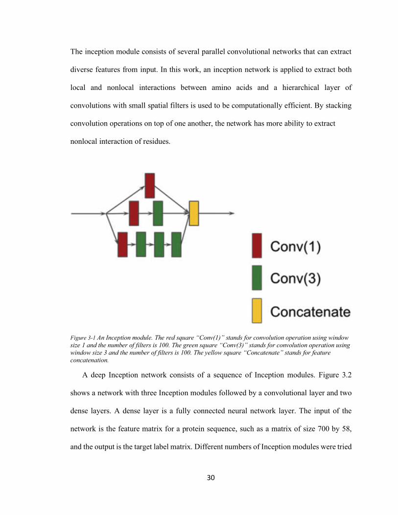
30
The inception module consists of several parallel convolutional networks that can extract
diverse features from input. In this work, an inception network is applied to extract both
local and nonlocal interactions between amino acids and a hierarchical layer of
convolutions with small spatial filters is used to be computationally efficient. By stacking
convolution operations on top of one another, the network has more ability to extract
nonlocal interaction of residues.
Figure 3-1 An Inception module. The red square “Conv(1)” stands for convolution operation using window size 1 and the number of filters is 100. The green square “Conv(3)” stands for convolution operation using window size 3 and the number of filters is 100. The yellow square “Concatenate” stands for feature concatenation.
A deep Inception network consists of a sequence of Inception modules. Figure 3.2
shows a network with three Inception modules followed by a convolutional layer and two
dense layers. A dense layer is a fully connected neural network layer. The input of the
network is the feature matrix for a protein sequence, such as a matrix of size 700 by 58,
and the output is the target label matrix. Different numbers of Inception modules were tried

31
in our experiments to find appropriate values for our prediction tasks. The deep neural
networks were implemented, trained, and experimented using TensorFlow (Abadi et al.,
2016) and Keras (Chollet, 2015; https://github.com/fchollet/keras).
Figure 3-2 A deep Inception network consisting of three Inception modules, followed by one convolution
and two fully-connected dense layers.
3.3 Newdeepinception-inside-inceptionnetworksforprotein
secondarystructureprediction(Deep3I)
In this section, a new deep Inception-Inside-Inception network architecture (Deep3I) is
presented. The architecture extends deep Inception networks through nested Inception
modules.
Figure 3.3 shows a deep Inception-Inside-Inception network (Deep3I) consisting of two
Deep3I blocks, followed by a convolutional layer and two dense layers. A Deep3I block is
constituted by a recursive construction of an Inception model inside another Inception
module. Stacked Inception modules could extract non-local interactions of residues over a

32
diverse range in a more effective way. Adding more Deep3I blocks is possible but requires
more memory.
Figure 3-3 A deep Inception-Inside-Inception (Deep3I) network that consists of two Deep3I blocks. Each
Deep3I block is a nested Inception network self. This network was used to generate the experimental results reported in this paper.
Each convolution layer, such as ‘Conv (3)’ in Figure 3.3, consists of four operations in
sequential order: 1) A one- dimensional convolution operation using the kernel size of
three; 2) The Batch normalization technique (Ioffe and Szegedy, 2015) for speeding up the
training process and acting as a regularizer; 3) The activation operation, ReLU (Radford et
al., 2015); and 4) The Dropout operation (Srivastava et al., 2014) to prevent the neural
network from overfitting by randomly dropping neurons during the deep network training
process so that the network can avoid co-adapting.
Deep3I networks were implemented, trained, and experimented using Tensorflow and
Keras. In our experiments, a large number of network parameters and training parameters
were tried. For the results reported, the dropout rate was set at 0.4. During training, the
learning rate scheduler from Keras was used to control the learning rate. The initial learning

33
rate was 0.0005, and after every 40 epochs, the learning rate dropped as shown by the
following formulas: 𝑙𝑟𝑎𝑡𝑒 = 0.0005 ∗ 𝑝𝑜𝑤(0.8, 𝑓𝑙𝑜𝑜𝑟(𝑒𝑝𝑜𝑐ℎ + 1)/40). An early stopping
mechanism from Keras was used to stop the network training when the monitored
validation quantity (such as validation loss and/or validation accuracy) stopped improving.
The “patience” (number of epochs with no improvement after which training was stopped)
was set as a number from 5 to 8. TensorBoard from Keras was used to visualize dynamic
graphs of the training and validation metrics.
The new Deep3I networks are different from existing deep neural networks. The
networks in (Li and Yu, 2016; Busia and Jaitly, 2017) consist of residual blocks and a
multi-scale layer containing convolutional layers with convolution window sizes of 3, 7,
and 9 to discover the protein local and global context. Although Deep3I uses convolution
window size of 1 or 3, through stacked deep convolution blocks, the network can represent
both local and global context well, while maintains efficient computation.
3.4 ExperimentalResults
In this section, extensive experimental results of the proposed deep neural networks on
multiple commonly used datasets and performance comparison with existing methods are
presented.
The following five publically available datasets were used in our experiments:
1) CullPDB dataset. CulPDB (Wang and Dunbrack, 2003) was downloaded on 15 June
2017 with 30% sequence identity cutoff, resolution cutoff 3.0Å and R-factor cutoff 0.25.
The raw CullPDB dataset contains 10,423 protein sequences. All sequences with length
shorter than 50 or longer than 700 were filtered out, which left the remaining 9972

34
protein sequences. CD-HIT (Fu et al., 2012) was then used to remove similar sequences
between CullPDB and CASP10, CASP11 and CSAP12 datasets. After that, there were
9589 proteins left. Among them, 8 protein sequences were ignored because they are too
short to generate PSI-BLAST profile. For the final 9581 proteins, 9000 were randomly
selected as the training set and the rest 581 as the validation set.
2) JPRED (Drozdetskiy et al., 2015) dataset. All proteins from the JPRED dataset belong
to different super-families, which gives the experimental result a more objective
evaluation.
3) CASP datasets. CASP10, CASP11 and CASP12 datasets were downloaded from the
official CASP website http://predictioncenter.org. The Critical Assessment of protein
Structure Prediction, or CASP, is a bi-annual worldwide experiment for protein structure
prediction since 1994. The CASP datasets have been widely used in the bioinformatics
community. To get the secondary structure labels of the proteins, the DSSP program
(Kabsch and Sander, 1983) was used. Some of the PDB files (including T0675, T0677
and T0754) could not generate the DSSP result; so, they were discarded. Some protein
sequences (including T0709, T0711, T0816 and T0820) are too short and PSI-BLAST
could not generate profiles; so, they were also removed. Finally, 98 out of 103 in
CASP10, 83 out of 85 in CASP11 and 40 out of 40 in CASP12 were used as our CASP
dataset.
4) CB513 benchmark (Zhou and Troyanskaya, 2014). This benchmark has been widely
used for testing and comparing the performance of secondary structure predictors.
5) Most recently PDB (Protein Data Bank). Because training data used in different tools
are not same, it is important to use PDB files that have not been seen by any previous

35
predictors (including ours) to objectively evaluate the performance. For this purpose,
the most recently published protein PDB files dated from July 1, 2017 to August 15,
2017 were downloaded. This set contains 614 proteins, each of which share <30%
sequence identity. Then, 385 proteins with a length between 50 and 700 were kept. To
perform a more objective test, each of the 385 proteins was searched against CullPDB
using BLAST and was classified into two categories: 1) easy cases where e-value is less
than or equal to 0.5; and 2) hard cases which can have no hit or e-value higher than 0.5.
After the classification, there are 270 easy cases and 115 hard cases.
In our experiments, the Deep3I configuration as shown in Fig. 3.3 was used to generate
the results reported in this article. In most cases, the CullPDB dataset was used to train
various deep neural networks, while the other datasets were only used in testing and
performance comparison with other methods and existing results.
3.4.1 PSI-BLASTvs.DELTA-BLAST
When generating the sequence profiles, most researchers (Zhou and Troyanskaya, 2014;
Wang et al., 2016; Li and Yu, 2016; Busia and Jaitly, 2017) chose PSI-BLAST (Altschul
et al., 1997), which can reliably generate a good protein sequence profiles. Besides PSI-
BLAST, other profile search tools are available, such as CS-BLAST (Biegert and Soding,
2009), DELTA_BLAST (Boratyn et al., 2012), PHI-BLAST (Zhang et al.,1998), etc. In
this work, the performance between two popular tools were compared: PSI-BLAST vs.
DELTA-BLAST on the JPRED dataset to decide which tool to use to generate the input
feature vectors for the new Deep3I network. For the PSI-BLAST experiment: both training
and test data profiles were generated by setting the e-value at 0.001, num_iterations at 3

36
and db is UniRef50. The JPRED dataset itself contains a training set of 1348 protein
sequences and a test set of 149 protein sequences. The JPRED training dataset was used to
train the Deep3I network and the JPRED test dataset was used to report the prediction Q3.
The Deep3I network were trained five times from random initial weights, and the average
Q3 accuracy and standard deviation are reported in Table 3.1. The same procedure was
used for DELTA-BLAST with its default search database (2017/4/1, with a size of 8.7GB).
The comparison of their results is shown in Table 3.1. Even though the average profile
generation time of DELTA-BLAST is faster than PSI-BLAST, the Q3 accuracy of Deep3I
using DELTA-BLAST is not as high as using PSI-BLAST. Hence, PSI-BLAST was
chosen to generate profiles in the rest of our experiments.
Table 3.1 Comparison of the profile generation execution time and Deep3I Q3 accuracy using PSI-BLAST and DELTA-BLAST
Tool avg. profile generation time (minutes) Q3 accuracy %
PSI-BLAST* 16.8(+/-10.14) 84.21(+/-0.49)
DELTA-BLAST 7.56(+/-3.96) 83.63(+/-0.31) *Database for PSI-BLAST search was UniRef50 download on 2017/4/12, 8.7GB.
3.4.2 Deep3Ivs.theBestExistingMethods
Many previous researchers (Busia et al., 2017; Li and Yu, 2016; Wang et al., 2016)
benchmarked their tools or methods using the dataset CB513 (Zhou and Troyaskaya,
2014). For a fair comparison, the same CullPDB dataset was used to train and test the
MUFOLD-SS in the same way as for existing methods reported in previous publications.
Table 3.2 shows the performance comparison between Deep3I and four of the best
existing methods (SSPro, DeepCNF-SS, DCRNN, and DCNN) in terms of the Q8

37
prediction accuracy on the CB513 dataset. All these methods were compared under the
condition of the same input and features. In this case, only the protein sequence and PSI-
BLAST profiles were provided. No additional technique like the next-step condition
proposed in (Busia et al., 2017) was involved. SSPro was run without using template
information. The result shows Deep3I obtained the highest accuracy.
Table 3.2 Q8 accuracy (%) comparison between MUFOLD-SS and existing state-of-the-art methods using the same sequence and profile of benchmark CB513.
Tool CB513 SSPro (Cheng et al., 2005) 63.5* DeepCNF-SS (Wang et al., 2016) 68.3* DCRNN (Li and Yu, 2016) 69.7* DCNN (Busia et al., 2017) 70.0** MUFOLD-SS 70.63 *Results reported by (Wang et al., 2016) **Results reported by (Busia et al., 2017)
Tables 3.3 and 3.4 show the performance comparison between MUFold-SS and the best
existing methods (SSPro, PSIPRED, DeepCNF-SS) in terms of the Q3 prediction accuracy
on the CASP datasets. PSIPRED could not predict 8-class classification, and thus do not
have result on Q8 accuracy.
Table 3.3 Q3 accuracy (%) comparison between MUFOLD-SS and other state-of-the-art methods on CASP datasets.
CASP10 P value CASP11 P value CASP12 P value PSIPRED 0.8390(±0.0731) 6.829e-5 0.8262(±0.0648) 0.0298 0.8051(±0.0905) 0.446 SSpro 0.7882(±0.0744) 3.315e-20 0.7826(±0.0632) 1.195e-14 0.7577(±0.0913) 2.169e-8 DeepCNF-SS 0.8386(±0.0657) 8.293e-7 0.8286(±0.0604) 0.0774 0.8131(±0.0771) 0.213 MUFOLD-SS 0.8598(±0.0683) - 0.8359(±0.0711) - 0.8059(±0.0933) - P values indicates the significance of the difference between MUFOLD-SS and PSIPRED/SSpro/DeepCNF-SS Table 3.4 Q8 accuracy (%) comparison between Deep3I and other state-of-the-art methods on CASP datasets.
CASP10 P value CASP11 P value CASP12 P value SSpro 0.6703(±0.0951) 1.347e-24 0.6651(±0.0820) 2.022e-21 0.6348(±0.1180) 1.584e-9 DeepCNF-SS 0.7403(±0.0933) 1.713e-8 0.7325(±0.0897) 0.133 0.7009(±0.1088) 0.334 MUFOLD-SS 0.7710(±0.0985) - 0.7392(±0.1008) - 0.7048(±0.1163) - P values indicates the significance of the difference between MUFOLD-SS and SSpro/DeepCNF-SS
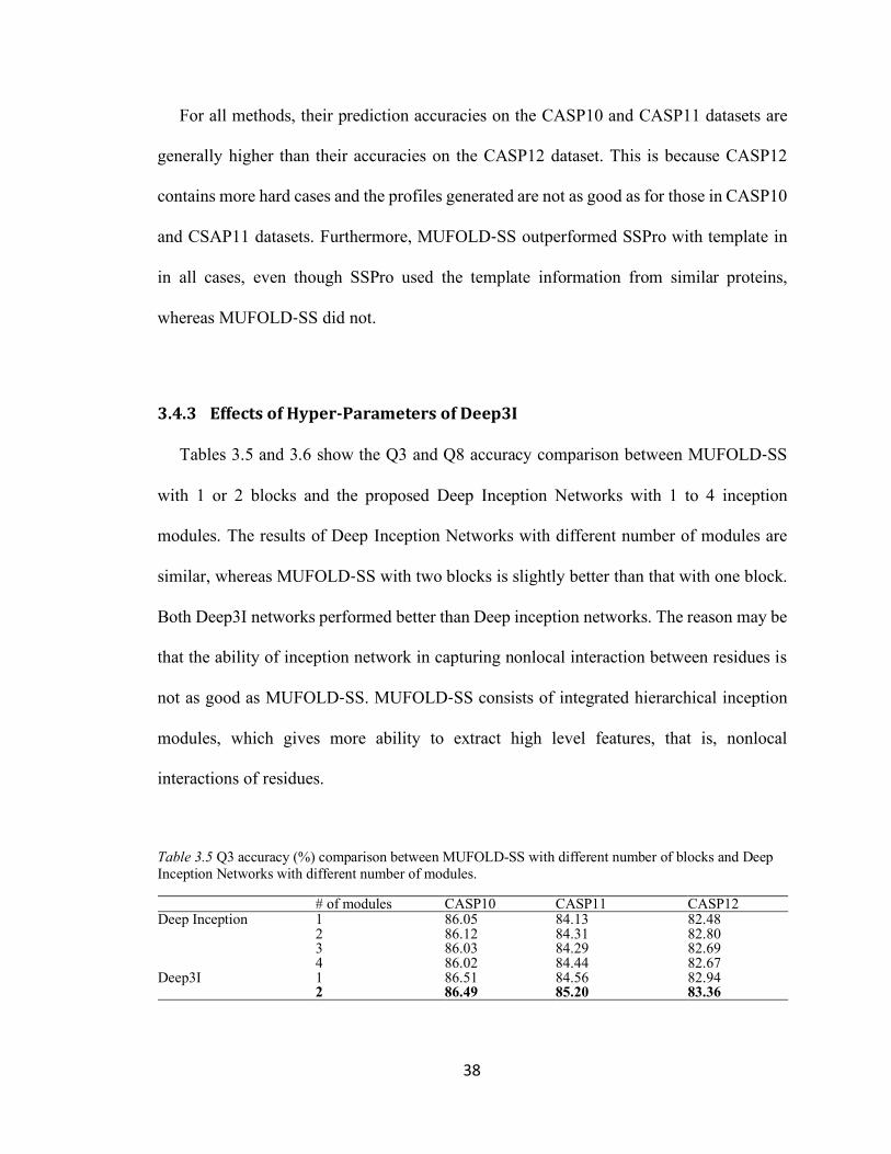
38
For all methods, their prediction accuracies on the CASP10 and CASP11 datasets are
generally higher than their accuracies on the CASP12 dataset. This is because CASP12
contains more hard cases and the profiles generated are not as good as for those in CASP10
and CSAP11 datasets. Furthermore, MUFOLD-SS outperformed SSPro with template in
in all cases, even though SSPro used the template information from similar proteins,
whereas MUFOLD-SS did not.
3.4.3 EffectsofHyper-ParametersofDeep3I
Tables 3.5 and 3.6 show the Q3 and Q8 accuracy comparison between MUFOLD-SS
with 1 or 2 blocks and the proposed Deep Inception Networks with 1 to 4 inception
modules. The results of Deep Inception Networks with different number of modules are
similar, whereas MUFOLD-SS with two blocks is slightly better than that with one block.
Both Deep3I networks performed better than Deep inception networks. The reason may be
that the ability of inception network in capturing nonlocal interaction between residues is
not as good as MUFOLD-SS. MUFOLD-SS consists of integrated hierarchical inception
modules, which gives more ability to extract high level features, that is, nonlocal
interactions of residues.
Table 3.5 Q3 accuracy (%) comparison between MUFOLD-SS with different number of blocks and Deep Inception Networks with different number of modules.
# of modules CASP10 CASP11 CASP12 Deep Inception 1 86.05 84.13 82.48
2 86.12 84.31 82.80 3 86.03 84.29 82.69 4 86.02 84.44 82.67
Deep3I 1 86.51 84.56 82.94 2 86.49 85.20 83.36
39
Table 3.6 Q8 accuracy (%) comparison between Deep3I with different number of blocks and Deep Inception Networks with different number of modules.
# of modules CASP10 CASP11 CASP12 Deep Inception 1 75.41 73.12 71.22
2 75.70 73.26 71.55 3 75.14 73.33 71.31
4 75.23 73.37 71.42 Deep3I 1 76.03 73.74 71.54 2 76.47 74.51 72.1
3.4.4 ResultsUsingMostRecentlyReleasedPDBFiles
The purpose of this test was to conduct a real-world testing, just like CASP, by using
the most recently published PDB protein files dated from July 1, 2017 to August 15, 2017.
These PDB files had not been viewed by any previous predictors. As mentioned before,
the most recently released PDB proteins were classified into two categories: the 270 easy
cases and 115 hard cases.
MUFOLD-SS is compared with the best available tools in this field, including
PSIPRED, SSPro, and the newly developed SPIDER3 on this set of data. Some protein
files in this dataset has special amino acid like ‘B’, which causes SPIDER3 prediction
failure. To make a fair comparison, proteins containing those special cases were excluded
(20 hard cases and 44 easy cases in total) and the remaining proteins were used as test cases
to compare the four tools. Again, MUFOLD-SS was trained using the CullPDB dataset and
tested on the new dataset.
Table 3.7 shows the performance comparison of the 4 tools. Again, Deep3I
outperformed the other state-of-the-art tools in both easy and hard cases. Different from
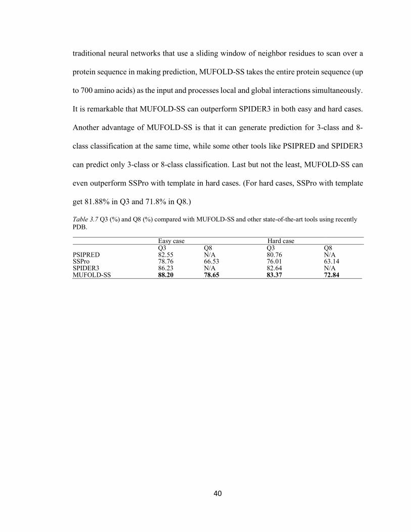
40
traditional neural networks that use a sliding window of neighbor residues to scan over a
protein sequence in making prediction, MUFOLD-SS takes the entire protein sequence (up
to 700 amino acids) as the input and processes local and global interactions simultaneously.
It is remarkable that MUFOLD-SS can outperform SPIDER3 in both easy and hard cases.
Another advantage of MUFOLD-SS is that it can generate prediction for 3-class and 8-
class classification at the same time, while some other tools like PSIPRED and SPIDER3
can predict only 3-class or 8-class classification. Last but not the least, MUFOLD-SS can
even outperform SSPro with template in hard cases. (For hard cases, SSPro with template
get 81.88% in Q3 and 71.8% in Q8.)
Table 3.7 Q3 (%) and Q8 (%) compared with MUFOLD-SS and other state-of-the-art tools using recently PDB.
Easy case Hard case Q3 Q8 Q3 Q8 PSIPRED 82.55 N/A 80.76 N/A SSPro 78.76 66.53 76.01 63.14 SPIDER3 86.23 N/A 82.64 N/A MUFOLD-SS 88.20 78.65 83.37 72.84

41
CHAPTER4 ANEWDEEPNEIGHBORRESIDUAL
NETWORKFORPROTEINSECONDARYSTRUCTURE
PREDICTION
4.1 DeepNRN–DeepNeighbor-ResidualNetwork
In this section, the proposed DeepNRN method is presented. Subsection 4.1.1 presents
its building block and network architecture. Subsection 4.1.2 describes some details in
training the network. Subsection 4.1.3 describes the input features to the network model.
Subsection 4.1.4 discusses the effect of applying different Struct2Struct networks and
different numbers of iterative training to fine-tune the network result.
4.1.1 DeepNRNArchitecture
Figure 4.1 shows the basic building block of DeepNRN, the neighbor residual unit,
which consists of a sequence of convolutions and concatenations with two shortcuts, and
the number of filters (feature planes) is 100. Since the convolutions with large spatial filters
are computationally expensive, we use a hierarchical layer of convolutions with small
spatial filters. A detailed explanation of factorization into smaller convolutions can be
found in (Szegedy et al., 2016) and (Szegedy et al., 2016). Besides that, residual shortcut
lines (He et al., 2016; He et al., 2016; Zhang et al., 2017; Huang et al., 2016) are used so
that the flow of information from a predecessor can be passed to the successor layers. The
reason behind this is discussed in (He et al., 2016) and (He et al., 2016) as deep network
architecture may cause the vanishing-gradient problem. The neighbor-residual design is
different from denseNet in (Huang et al., 2016) in that the latter network with L layers can

42
have as many as 𝐿(𝐿 + 1)/2 direct connections, which may lead to an explosion of feature-
maps and consume large computational resources. Our network connection design is not
as dense as denseNet but still preserves the long distance of four (far neighbor) and short
distance of two (near neighbor) connections. This design can also alleviate the vanishing-
gradient problem for deep neural networks and reduce the burden of propagating large
feature-maps to the deeper layer comparing with the network flow of denseNet.
Figure 4-1 The basic building block of DeepNRN, i.e., neighbour-residual unit. The square “Conv3” stands for convolution operation using a window size 3, while the square “Concatenate” stands for feature
concatenation.

43
Figure 4.2 shows a neighbor-residual block that consists of five neighbor-residual units
strung together. The output of one neighbor-residual unit is the input to the next neighbor-
residual unit.
Figure 4-2 Neighbour-residual block has stacks of neighbor-residual units.
Figure 4.3 shows the overall DeepNRN architecture that consists of three neighbor-
residual blocks with size-3 convolutions in between, followed by one size 11 convolution
layer, and two dense fully-connected layers. Before each neighbor-residual block, the size-
3 convolutional layer acts as a transition. The input of the network is the sequence and
profiles. The output is the predicted secondary structure labels. We explored many other
ways of placing residual shortcuts between neighbor-residual blocks, and different
numbers of neighbor-residual blocks. Empirically, the architecture shown in Figure 4.3
works the best.
Figure 4-3 Deep neighbor-residual network (DeepNRN) architecture.

44
4.1.2 BatchNormalizationandDropout
The TensorFlow 1.0 version (Abadi et al., 2016) and the Keras 2.0 version (Chollet,
2015) of machine learning environments were used for training the DeepNRN networks.
To speed up the training, batch normalization (Ioffe and Szegedy, 2015) was applied after
convolutions, which also acted as a regularizer. The rectified linear unit (ReLU) (Zeiler et
al., 2013), as the activation function, was used after batch normalization. To reduce
network overfitting, dropout (Srivastava et al., 2014) was added after the activation layer.
Several dropout ratios, ranging from 0.3 to 0.8, were tested in our experiments and the
value 0.4 was used in our final experiments. Adam optimization (Kingma and Ba, 2014)
was used to train the networks. The learning rate scheduler from Keras was used to control
the learning rate. The validation loss was monitored and used to early-stop the training
process to avoid overfitting. The early-stopping “patience” (i.e., the number of epochs with
no improvement after which training was stopped) was set between 8 to 12 in experiments,
case by case. The experiments were performed on an Alienware Area desktop computer
with a Titan-X GPU card equipped.
4.1.3 InputFeatures
The input features to DeepNRN consists of a protein sequence and its profiles generated
by PSI-BLAST (Altschul et al., 1997) and HHBlits (Remmert et al., 2012), respectively.
One-hot vector encoding was used to represent protein sequences. To be consistent with
the position specific scoring matrix (PSSM) results were generated by PSI-BLAST, which
contains only 20 different kinds of amino acids, some special cases were handled as
followed: Amino acid ‘X’ is treated like amino acid ‘A’; ‘B’ is like ‘N’; and ‘Z’ is like ‘Q’.

45
The input length of the amino acid sequence was fixed at 700. If a protein sequence is
shorter than 700, a ‘NoSeq’ label is padded to the end of the sequence, which means no
amino acid is there. If a protein sequence is longer than 700, it is broken into segments
shorter than 700. In the implementation, a protein sequence is represented as a 700-by-21
(20 amino acids + NoSeq label) array. Next, protein profiles were generated using PSI-
BLAST (Altschul et al., 1997) and HHBlits (Remmert et al., 2012), respectively, like the
previous work in (Wang et al., 2016; Heffernan et al., 2017). The PSI-BLAST tool
parameters were set to (evalue 0.001, num_iterations 3, and db UniRef50) to generate
PSSM. PSSM values were then converted to the range (0, 1) through the Sigmoid function.
The PSI-BLAST profile information is represented as a 700-by-21 array. The HHBlits tool
parameters are set to (d uniprot20_2013_03, maxres 40 000, Z 0) to generate HHM profiles.
The HHM files are represented as a 700-by-30 array and the information retrieved from
HHM is processed the same as in (Heffernan et al., 2017): Convert ‘*’ to 0 and other non-
‘*’ value to 𝑓(𝑥) = 2xyz{{{. By combining the three arrays together. The final input to
DeepNRN is a 700-by-72 array.
4.1.4 Struct2StructNetworkandIterativeFine-tuning
The Struct2Struct network proposed by (Rost and Sander., 1993) was added after the
DeepNRN network to fine-tune the predicted results and take into consideration the
consecutive patterns. For example: a-helix should consist of at least 3 consecutive patterns.
The predicted secondary structure from DeepNRN may violate such a pattern, i.e. not
protein-like. The initial testing predicted that secondary structures are fine-tuned and more
protein-like after passing through the Struct2Struct network.

46
Heffernan et al. (2017) employed an iterative learning process in their protein secondary
structure prediction. We adopted a similar approach, but only on the fine-tuning part, i.e.,
we iteratively fine-tuned the Struct2Struct network. One of the inputs to the Struct2Struct
network is the output from a previous DeepNRN prediction, i.e., the predicted probability
of each class from the last Softmax layer, and another input to the Struct2Struct network is
the physico-chemical properties (PP) of amino acids (Heffernan et al., 2017). The output
of the Struct2Struct network is again the secondary structure labels. This fine-tuning
process can be iteratively repeated, which takes the predicted output from the Struct2Struct
network and feeds it back into the network as its input.
The existing Struct2Struct network described in (Rost and Sander, 1993) used single-
layer neural networks. In our work, different size convolution kernels were tested and, in
the end, size 21 was chosen based on the fine-tuning performance. The Struct2Struct
network may not improve the prediction accuracy much, but it can make the prediction
more protein like and increase prediction accuracy of some small classes, such as B, G, S,
T.
In summary, the proposed DeepNRN method is different from existing methods. The
DeepNRN architecture differs from Busia’s (Busia and Jaitly, 2017) and Li’s (Li and Yu,
2016) architecture in that (Li and Yu, 2016) used residual blocks and multi-scale layer
containing CNN layers with convolution window sizes of 3, 7, and 9 to discover protein
local and global context. In contrast, DeepNRN consists of stacked CNN layers with a
convolution window size 3 only. When deep convolution blocks are stacked, they can
capture both short- and long-range sequence information. DeepNRN is also different from
Heffernan’s network (Heffernan et al., 2017), where the latter applied long short-term

47
memory (LSTM) (Sak et al., 2014) and a bidirectional neural network (BiNN) to perform
the global context extraction. Furthermore, the key advantage of DeepNRN, the near and
far neighbor residual connections, can reduce the vanishing-gradient problem in deep
networks and strengthen the feature propagation. The Struct2Struct network was added
after the DeepNRN network because fine-tuning makes the prediction results more protein-
like.
4.2 ExperimentalResults
In our experiments, three public data sets were used: (1) the CullPDB (Wang and
Dunbrack, 2003) preprocessed data set from (Li and Yu, 2016) and (Busia and Jaitly,
2017); (2) the CB513 benchmark in (Li and Yu, 2016) and (Busia and Jaitly, 2017); (3)
CASP10, CASP11 and CASP12 data sets (http://predictioncenter.org/). The CullPDB data
set was used to train the deep networks, while the other data sets were used for testing and
comparison with other state-of-the-art tools. Please note that the CullPDB data set from
(Zhou and Troyanskaya, 2014) was constructed before January 2014 and any two proteins
in this set share less than 25% sequence identity with each other. Originally, this CullPDB
had 6128 proteins. We used the filtered CullPDB data set, in which the sequence identity
with the CB513 test data is less than 25%. The filtered CullPDB data set contains 5534
protein sequences, and 5278 of them were randomly selected to form the training set and
the remaining 256 sequences form the validation set.
As in (Li and Yu, 2016) and (Busia and Jaitly, 2017), the Q3 and Q8 accuracies were
used as the performance metrics in evaluation. The Q3 or Q8 accuracy measures the
percentage of residues being correctly predicted among three-state or eight-state protein

48
secondary structure classes. In addition, the Matthew correlation coefficient (Matthews,
1975) was used, as it provides a more balanced measurement of classification quality.
4.2.1 PerformanceComparisonofDeepNRNwithOtherState-of-the-artTools
BasedontheCB513Dataset
In our experiments, two widely used state-of-the-art tools, SCRATCH_1D (SSPro ab
initio) (Cheng et al., 2005), (Magnan et al., 2014) and Psipred (Jones, 1999) were used to
compare their performance with that of DeepNRN on the data set CB513. For a fair
comparison, the same PSI-BLAST data base (a smaller version of UniRef50 included in
the SSPro package) was used by all three methods. SSPro contains the legacy Blast 2.2.26
for profile searches. Since Psipred does not contain PSI-BLAST, the legacy Blast 2.2.26
was installed for it. The new Blast+ package 2.6.0+ was used in our DeepNRN system.
Table 4.1 shows the Q3 and Q8 results of all three methods. The new DeepNRN method
outperforms the other two methods by a large margin.
Table 4.1 Performance comparison of DeepNRN, SSPro, and PSIPRED on Q3 and Q8 accuracy on the CB513 data set.
Q3 (%) Q8 (%)
SSPro 78.6 66.5
Psipred 79.2 N/A
DeepNRN 83.7 71.1

49
4.2.2 PerformanceComparisonofDeepNRNwithOtherState-of-the-artTools
BasedonFourWidelyUsedDatasets
In this set of experiments, the results of DeepNRN were compared with published
results of other state-of-the-art methods in (Zhou and Troyanskaya, 2014) and (Wang et
al., 2016) on CB513, as well as three data sets from the world-wide contest of protein
structure prediction, i.e., the Critical Assessment of Protein Structure Prediction (CASP).
To prepare the data sets, we downloaded the PDB files from the official CASP website
http://prediction-center.org/. Note that some of the PDB files provided do not have
corresponding FASTA files. For example, T0644.fasta contains 166 amino acids; however,
T0644.pdb contains only 141 amino acids. To be consistent, protein sequences were
extracted from PDB; then, the DSSP program (Touw et al., 2015; Kabsch and Sander,
1983) was used to retrieve the ground truth secondary structure for those extracted
sequences. Some of the PDB files, including T0675, T0677 and T0754, could not generate
the DSSP output; so, they were discarded. Some protein sequences, including T0709,
T0711, T0816 and T0820, were too short to have any PSI-BLAST hit; so, they were
removed as well. Overall, the proteins used in the experiments were CASP10 (98 out of
103), CASP11 (83 out of 85) and CASP 12 (40 out of 40).
Tables 4.2 and 4.3 show the Q3 and Q8 accuracy results, respectively, of various
methods. Bold-face numbers in each column represent the best result on a particular data
set, and ‘-’ denotes that no result was available. The results show that DeepNRN is
significantly better than previous methods in all cases, except for Q3 on CASP11, where
DeepCNF-SS is slightly better.
Table 4.2 Q3 (%) accuracy results of various prediction methods on four data sets.

50
CB513 CASP10 CASP11 CASP12
SSPro* 78.5 78.5 78.6 76.0**
SPINE-X* 78.9 80.7 79.3 -
PSIPRED* 79.2 81.2 80.7 80.3**
JPRED* 81.7 81.6 80.4 -
RaptorX-SS8* 78.3 78.9 79.1 -
DeepCNF-SS* 82.3 84.4 84.7 -
DeepNRN** 83.7 85.6 83.6 81.6
*Results reported in (Wang et al., 2016). ** Our experimental results.
Table 4.3 Q8 (%) accuracy results of various prediction methods on four data sets.
CB513 CASP10 CASP11 CASP12
SSPro* 63.5 64.9 65.6 63.1**
RaptorX-SS8* 64.9 64.8 65.1 -
DeepCNF-SS* 68.3 71.8 72.3 -
DeepNRN** 71.1 75.33 72.9 70.8
* Results reported in (Wang et al., 2016). ** Our experimental results.
4.2.3 EffectofConvolutionWindowSizeinStruct2StructNetworkand
IterativeRefinement
The Struct2Struct network was implemented as a convolutional layer, and different
convolutional window sizes were tried to find out its effect on the results. Figures 4.4 and
4.5 show the effects of different convolutional window sizes and iterative refinement using
repeated Struct2Struct networks on Q8 and Q3 accuracies, respectively. As shown in Fig.

51
4.4(a) and 4.5(a), the general trend is that the accuracies decrease slightly as the number of
iterations increases, and a large window size leads to lower accuracy. Occasionally, the
accuracy could increase slightly, as in the case of window size 21 after one iteration of
fine-tuning on Q8. More iterations may not necessarily increase the fine-tuning results, but
the accuracy will drop. The reason may lie in too much iterative training causing the
network to become over-trained, and causing the performance to drop. The convolutional
window size is a way of considering near-intermediate interactions of residues. From the
experiment results, a window size was chosen between 15 and 21, which is reasonable, on
a case by case basis, depending on the problem. If the window was too small, not enough
neighboring residues could cover and the purpose of Struct2Struct was to take into
consideration the consecutive neighboring residues.
Figures 4.4(b) and 4.5(b) compare the confusion matrices of the prediction results of
DeepNRN alone vs. an additional Strut2Struct network layer of window-size 21. Although
the added Struct2Struct network did not significantly change Q3 and Q8 accuracy, more
instances of the smaller classes, including B, G, S and T, were correctly predicted for Q8.
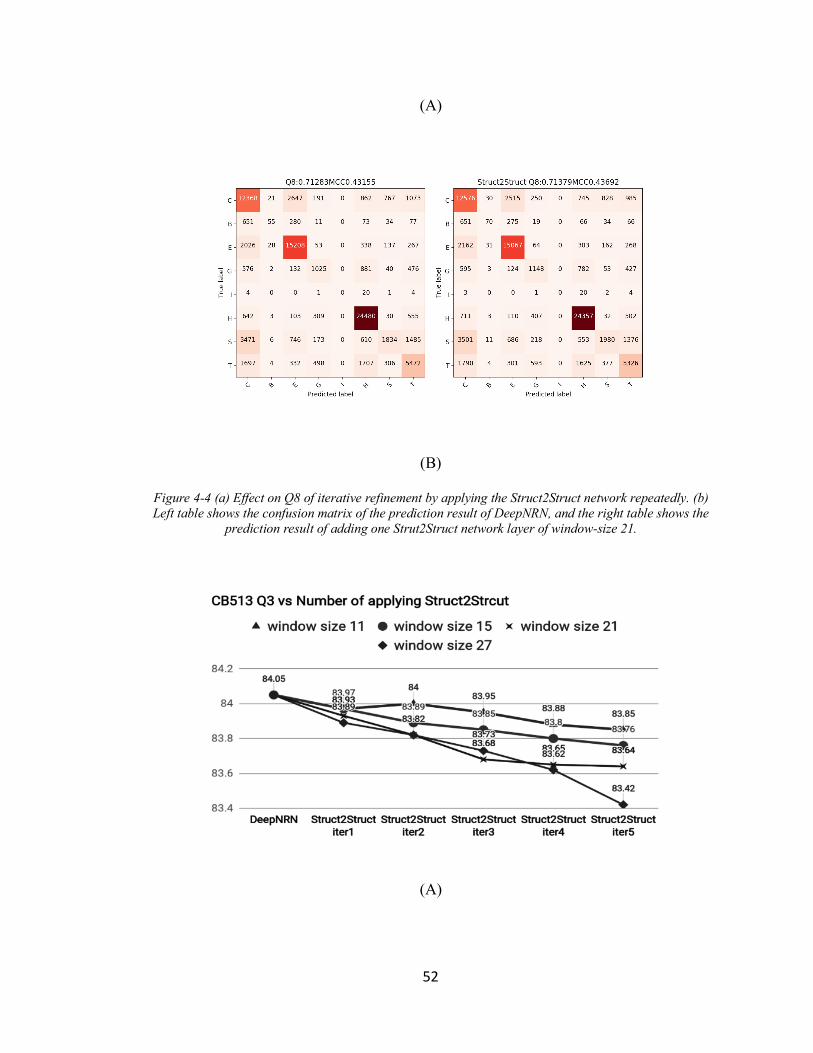
52
(A)
(B)
Figure 4-4 (a) Effect on Q8 of iterative refinement by applying the Struct2Struct network repeatedly. (b) Left table shows the confusion matrix of the prediction result of DeepNRN, and the right table shows the
prediction result of adding one Strut2Struct network layer of window-size 21.
(A)

53
(B)
Figure 4-5 (a) Effect on Q3 of iterative refinement by repeatedly applying Struct2Struct network. (b) Left table shows the confusion matrix of the prediction result of DeepNRN, and the right table shows the
prediction result of adding one Struct2Struct network layer of window-size 21.
4.2.4 ExplorationofotherNetworkConfigurationsofDeepNRN
Other configurations of DeepNRN design were explored, and the performance was
tested and compared in Table 4.4. As the experiment results show, the neighbor shortcuts
played a very important role in propagating a large feature map to deep layers of networks
because without them, the performance dropped. The far-neighbor shortcuts were also very
important as shown in Table IV; without them, the performance dropped significantly.
Also, adding more NRN blocks was possible but consumed more computational resources,
e.g., GPU memory.
Table 4.4 Other Network Configuration of DeepNRN and Performance

54
CB513
Without near neighbor shortcuts 70.8 Without far neighbor shortcuts 62.7 1 NRN Block 70.4 2 NRN Blocks 70.7 DeepNRN 71.1

55
CHAPTER5 PROTEINBACKBONETORSIONANGLES
PREDICTIONUSINGDEEPRESIDUALINCEPTION
NETWORKS
5.1 Problemformulation
For a given amino acid sequence of a protein, the goal is to predict the backbone torsion
angles (Psi and Phi) of each residue. Psi is the N(i), Ca(i), C(i), N(i+1) torsion angle for
residue i and Phi is the C(i-1), N(i), Ca(i), C(i) torsion angle for residue i (see Figure 1.1).
The ranges of Psi-Phi angle are between -180 to 180 degrees. It is important to feed the
deep neural networks with useful inputs in order to make accurate prediction. In the
proposed method, the input is designed to include as much useful information that can be
obtained or generated based on the amino acid sequence. Specifically, the input features
consist of physico-chemical properties of amino acids, PSI-BLAST profile, HHBlits
profile, and predicted secondary structures. Figure 5.1 shows an example of the physico-
chemical feature vector. Each amino acid in the protein sequence is represented as a vector
of 8 real numbers ranging from -1 to 1. The vector consists of the seven physico-chemical
properties as in (Fauchere et al., 2009) plus a number 0 or 1 representing the existence of
an amino acid at this position as an input (called NoSeq label). The reason of adding the
NoSeq label is because the proposed deep neural networks are designed to take a fixed size
input, such as a sequence of length 700 residues in our experiment. Then, to run a protein
sequence shorter than 700 through the network, the protein sequence will be padded at the
end with 0 values and the NoSeq label is set to 1. For example, if the length of a protein is
500, then the first 500 rows are similar to the example in Figure 5.1 with NoSeq label set

56
to 0 and the last 200 rows have 0 values in the first 7 columns and 1 in the last column. If
the protein is longer than 700 residues, it can be split into multiple segments, each shorter
than 700 residues.
Figure 5-1 An example of the physico-chemical feature vector of a protein sequence. Each amino acid in the protein sequence is represented as a vector of 8 real numbers ranging from -1 to 1. The feature vectors
of the first 5 amino acids are shown.
The second set of features comes from the protein profiles generated using PSI-BLAST
(Altschul et al., 1999). In our experiments, the PSI-BLAST parameters were set to (evalue:
0.001; num_iterations: 3; db: UniRef50) to generate PSSM, which was then transformed
by the sigmoid function S(x) = 1/(1 + e5~) into the range (0, 1). Figure 5.2 shows an
example of the PSI-BLAST profile. Each amino acid in the protein sequence is represented
as a vector of 21 real values ranging from 0 to 1, representing the 20 amino acids PSSM
values plus a NoSeq label in the last column.
The third set of features comes from the protein profiles generated using HHBlits
(Remmert et al., 2011). In our experiments, the HHBlits software used database
uniprot20_2013_03, which can be downloaded from
http://wwwuser.gwdg.de/~compbiol/data/hhsuite/databases/hhsuite_dbs/. Again, the
profile values were transformed by the sigmoid function into the range (0, 1). Figure 5.3
shows an example of the HHBlits profile. Each amino acid in the protein sequence is

57
represented as a vector of 31 real numbers, of which 30 from amino acids HHM profile
values and 1 NoSeq label in the last column.
The fourth set of features comes from the predicted eight-class secondary structures by
DeepRIN itself. In our experiment, DeepRIN first takes the above-mentioned three sets of
features as input to predict the eight-class secondary structure features. The prediction
result is used as the fourth set of features for Psi-Phi angle prediction. The secondary
structure prediction result is a vector of nine numbers, of which the first eight are the
probabilities of the eight secondary structure classes and the last one is the NoSeq label.
Figure 5-2 An example of the PSI-BLAST profile of a protein sequence. Each amino acid in the protein sequence is represented as a vector of 21 real numbers ranging from 0 to 1. The feature vectors of the first
5 amino acids are shown. The third through the 19th columns are omitted.
Figure 5-3 An example of the HHBlits profile of a protein sequence. Each amino acid in the protein sequence is represented by a vector of 31 real values ranging from 0 to 1. The feature vectors of the first 5
amino acids are shown.

58
The four sets of features are combine into one feature vector of length 66 for each amino
acid as the input to our proposed deep neural networks. For the deep neural networks that
take the fixed-size input, the input feature matrix would be of size 700 by 66.
The new deep neural network will not predict Psi-Phi angle values directly. Instead, the
outputs for each amino acid positon are sin(𝜙), cos(𝜙), sin(𝜑), and cos(𝜑), in order to
remove the effect of angle’s periodicity. The predicted angles can be calculated by using
the sine and cosine predictions via equation 𝛼 = 𝑡𝑎𝑛5H[𝑠𝑖𝑛 𝛼 / 𝑐𝑜𝑠 𝛼].
5.2 NewDeepResidualInceptionNetworks(DeepRIN)forTorsion
AnglePrediction
In this section, a new deep inception residual network architecture is proposed for
protein torsion angle prediction. The architecture consists of stringed inception modules
and shortcut lines followed by some convolution and fully connected dense layers. Figure
5.4 shows the basic residual inception module of DeepRIN, which is designed based on
InceptionNet (Szegedy et al., 2017) and ResNet (He et al., 2016). The residual inception
module consists of two stacked inception modules to extract diverse features from the
input. Convolutions with small windows are used to make the networks computationally
efficient. The shortcut through Conv1 is designed to propagate feature maps into deeper
layers of the network to address the vanishing-gradient problem.

59
Figure 5-4 A residual-inception module of DeepRIN. The green rhombus “Conv(1)” denotes a convolution operation using window size 1 and the number of filters is 100. The orange square “Conv(3)” denotes a convolution operation using window size 3 and the number of filers is 100. The blue oval “Concatenate”
denotes feature concatenation.
Figure 5.5 shows two DeepRIN networks with two residual inception modules followed
by a convolutional layer and two dense layers. The first one predicts 8-class secondary
structure and the second one predicts torsion angles. The input of the first network is a
700x58 feature matrix of the given protein sequence of length 700, whereas the input of
the second network is a 700x66 feature matrix of the given protein sequence. Different
numbers of residual inception modules were tried and compared in our experiments to find
optimal values for our prediction tasks. The deep neural networks were implemented,
trained, and experimented using TensorFlow (Abadi et al., 2016) and Keras (Chollet,
2015).

60
Figure 5-5 Architecture of the proposed deep residual inception network architecture (DeepRIN).
Each convolution layer, such as ‘Conv (3)’ in Figure 5.5, consists of four operations in
the following sequential order: 1) A one-dimensional convolution operation using the
kernel size of three; 2) the batch normalization technique (Ioffe and Szegedy, 2015) for
speeding up the training process and acting as a regularizer; 3) the activation operation,
ReLU (Radford et al., 2015), for nonlinear transformation; and 4) the dropout operation
(Srivastava et al., 2014) to prevent the neural network from overfitting by randomly
dropping connections during the deep network training process so that the network can
avoid coadapting.
In our experiments, a large number of network parameters and training parameters were
tried. For the experimental results reported in the next section, the dropout rate was set at
0.4. During training, the learning rate scheduler from Keras was used to control the learning
rate. The initial learning rate was 0.0005, and after every 40 epochs, the learning rate
dropped as shown by the following formulas:𝑙𝑒𝑎𝑟𝑛𝑖𝑛𝑔𝑟𝑎𝑡𝑒 = 0.001 ∗

61
𝑝𝑜𝑤(0.8, 𝑓𝑙𝑜𝑜𝑟(𝑒𝑝𝑜𝑐ℎ + 1)/40). An early stopping mechanism from Keras was used to
stop training when the monitored validation performance (such as validation loss and/or
validation accuracy) stopped improving. The “patience” (number of epochs with no
improvement after which the training was stopped) was set between 5 and 8. The activation
function used for the last layer is tanh, as the predicted sine and cosine value should be
within the range [-1,1].
The new DeepRIN networks are different from existing deep neural networks. The
networks in (Heffernan et al., 2017) consisted of stacked RNN and iterative training, while
in DeepRIN, a stacked inception module and residual shortcuts were used to capture both
local and global interactions between residues efficiently. Also, DeepRIN is different from
DReRBM and DRNN in (Li et al., 2017) because they used a sliding window to create
input to deep neural networks, which is unable to capture long-range interactions between
amino acids. In DeepRIN, the input is the entire protein sequence.
At a convolutional layer, the previous layer’s feature maps are convolved with learnable
kernels and go through the activation function to generate the output feature map. The
convolution operation can be expressed in the following formulas:
𝒙?R = 𝑓(� 𝒙$R5H ∗ 𝒌$?R + 𝑏?R$∈�B
)
where 𝑀? represents a selection of input maps, b is bias, k is kernel, and x is feature maps.
The cross-entropy loss function used during the training is defined as following:
𝐿𝑜𝑠𝑠(𝑤) =1𝑁�𝐻(𝑝� − 𝑞�)
�
�GH

62
= −1𝑁�
(𝑦�𝑙𝑜𝑔𝑦�� + (1 − 𝑦�)log(1 − 𝑦��))�
�GH
where 𝑦�� = 1/(1 + 𝑒5�∗��), N is the total number of samples, w is the vector of weights,
the true probability p represents the percentage of the true labels, the given distribution q
is the predicted value of the current model, and x is the input vector.
5.3 ExperimentalResults
This section presents experimental results of the proposed deep neural networks on
multiple benchmarks in comparison with the best existing methods. The following four
publically available datasets were used in our experiments:
1) CullPDB dataset. CullPDB (Wang and Dunbrack, 2006) was downloaded on 15
June 2017 with 30% sequence identity cutoff, resolution cutoff 3.0Å and R-factor
cutoff 0.25. The raw CullPDB dataset contains 10,423 protein sequences. All
sequences with length shorter than 50 or longer than 700 were filtered out, which
left the remaining 9972 protein sequences. CD-HIT (Li and Godzik, 2006) was then
used to remove similar sequences between CullPDB and CASP10, CASP11 and
CASP12 datasets. After that, there were 9589 proteins left. Among them, 8 protein
sequences were ignored because they are too short to generate PSI-BLAST profiles.
For the final 9581 proteins, 9000 were randomly selected as the training set and the
rest 581 as the validation set.
2) CASP datasets. CASP10, CASP11 and CASP12 datasets were downloaded from
the official CASP website http://predictioncenter.org. The Critical Assessment of
protein Structure Prediction, or CASP, is a bi-annual worldwide experiment for

63
protein structure prediction since 1994. The CASP datasets have been widely used
in the bioinformatics community. To get the secondary structure labels of the
proteins, the DSSP program (Kabsch and Sander, 1983) was used. Some of the
PDB files (including T0675, T0677 and T0754) could not generate the DSSP
results, and hence they were discarded. Some protein sequences (including T0709,
T0711, T0816 and T0820) are too short and PSI-BLAST could not generate profiles
so that they were also removed. Finally, 98 out of 103 in CASP10, 83 out of 85 in
CASP11 and 40 out of 40 in CASP12 were used as our CASP dataset.
3) Recently released PDB proteins. Because different tools used different training
data, it is important to use PDB (Protein Data Bank) files that have not been seen
by any previous predictors (including ours) to objectively compare their
performance. For this purpose, recently published protein PDB files dated from
2017-7-1 to 2017-8-15 were downloaded. This set contains 614 proteins, each of
which share less than 30% sequence identity. Then, 385 proteins with a length
between 50 and 700 were kept. To perform a more objective test, each of the 385
proteins was searched against CullPDB using BLAST and was classified into two
categories: 1) easy cases where e-value is less than or equal to 0.5; and 2) hard cases
which have no hit or e-value higher than 0.5. After the classification, there are 270
easy cases and 115 hard cases.
4) SPIDER3’s training and test datasets. These datasets are available from
http://sparks-lab.org/server/SPIDER3/. The training data was used to train our
model, and the test set performance was reported and compared with SPIDER3. In
this experiment, only the sequences with length less than 700 residues were

64
retained. In total 4532 out of 4590 training cases were used to train our DeepRIN
model, and 1174 out of 1199 test cases were used to benchmark SPIDER3 and
DeepRIN.
In our experiment, the DeepRIN configuration shown in Figure 6 was used to generate
the results reported in this paper. The DeepRIN networks consisted of two inception blocks
and short-cut connected by residual network. We tried some different hyper-parameters,
such as different numbers of inception blocks (ranging from 1 to 5), in our experiments.
The configuration in Figure 5.5 worked well in general and used in the final networks.
In most cases, the CullPDB dataset was used to train various deep neural networks,
while the other datasets were only used in testing and performance comparison of different
methods and with results in the literature.
The Psi-Phi angle prediction was evaluated by the mean absolute error (MAE) between
the truth angle (𝐴$����)and the predicted angle (𝐴$����) for each residue i. To remove the
periodicity in angles, the error in prediction of residue i is defined as the smaller value of
𝑑$and 360–𝑑$, where 𝑑$ = �𝐴$���� − 𝐴$�����. In addition, Peasron Correlation Coefficient
was also used to evaluate the predicted Psi-Phi angles.
Table 5.1 compares the prediction results of DeepRIN and the best methods published
in (Li et al., 2017) using the same test dataset. In (Li et al., 2017), Li et al. proposed
DReRBM, which is a deep recurrent restricted Boltzmann machine (Nair and Hinton,
2010) and DRNN, which is a deep recurrent neural network (Mikolov et al., 2010) to
predict backbone torsion angle. SPIDER2 and SPIDER3 are two well-known tools
representing the state-of-the-art. The testset contains 11 free modeling targets selected from
CASP12 as described in (Li et al., 2017). The results show that DeepRIN outperformed all

65
existing methods significantly, reducing the Psi MAE by over 2.6 degree over the second
best, DReRBM, and the Phi MAE by nearly 1 degree over the second best, SPIDER3.
Table 5.1 Comparison of mean absolute errors (MAE) of Psi-Phi angle prediction between DeepRIN and best existing predictors using the test sets from (Li et al., 2017)
Psi MAE Phi MAE DReRBM (Li et al., 2017) * 35.99 22.47
DRNN (Li et al., 2017) * 37.54 22.38 SPIDER2* 37.67 22.61 SPIDER3 39.06 21.24 DeepRIN 33.34 20.30
*Published results in (Li et al., 2017)
Table 5.2 compares the results of DeepRIN, SPIDER2 and SPIDER3 on three datasets,
CASP10, CASP11 and CASP12. Again, DeepRIN outperformed SPIDER2 and SPIDER3
in all cases. The improvements are significant, reducing Psi angle prediction error by more
than 5 degrees and Phi angle prediction error by more than 1.5 degrees. The improvement
on the CASP12 dataset is slightly less than those on CASP10 and CASP11 datasets, which
may be because targets in CASP12 are harder targets and PSI-BLAST or HHblits did not
generate good profiles for them.
Table 5.2 Comparison of mean absolute errors (MAE) and Pearson Correlation Coefficient (PCC) of Psi-Phi angle prediction between DeepRIN, SPIDER2 and SPIDER3 using the CASP10, 11 and 12 datasets. The PCC is written in parentheses. Bold-font numbers in each column represent the best result on a particular dataset.
Angle CASP10 CASP11 CASP12 SPIDER2 Psi 49.18 (0.693) 48.13 (0.699) 50.59 (0.688)
Phi 25.83 (0.766) 26.06 (0.756) 26.85 (0.758) SPIDER3 Psi 31.17 (0.824) 33.05 (0.805) 35.67 (0.783)
Phi 20.41 (0.831) 21.38 (0.815) 21.12 (0.809) DeepRIN Psi 25.79 (0.861) 27.96 (0.841) 31.39 (0.813)
Phi 17.39 (0.874) 18.97 (0.853) 20.21 (0.838)
Figure 5.6 shows the average Psi-Phi angle prediction errors (MAEs) of DeepRIN for
protein targets in the CASP12 dataset across eight types of secondary structures, which are
310-helix (G), a-helix (H), p-helix (I), b-strand (E), b-bridge (B), b-turn (T), bend (S) and
loop or irregular (L). The result shows that for H (Helix), Psi-Phi angle prediction errors

66
are the lowest, yet the errors for T (Turn), S (Bend) and C (Loop Region) are the highest.
There is no “I” region in the targets.
Figure 5.7 shows the detailed Psi-Phi angle prediction results of two proteins in
CASP12: T0860 and T0861. Predicted angle value, true angle value, and absolute error are
plotted for each amino acid position, with its true secondary structure type labelled. T0860
is an example of hard cases with higher prediction errors, whereas T0861 is an example of
accurate prediction. The H (helix) regions generally have lower prediction errors, whereas
the C (coil) regions usually are harder to predict.
As shown in Figures 5.6 and 5.7, loop regions (T, S, C) generally have large prediction
errors. The H (Helix) regions and strand (E) regions can be predicted accurately.
Sometimes, Psi angles in beta sheets were predicted 180-degree reversely. For Phi angles,
the predictions are relatively better in helix and beta sheet regions. T0861 was predicted
quite well except for some turn and loop regions. An observation is that when the Psi-Phi
angles were predicted relatively well, the variance of the predicted Psi-Phi angles were
relatively large, as it captured the diversity of different angles. When the Psi-Phi angles
were not predicted accurately, the predicted angles had smaller variations.
Table 5.3 compares the results of DeepRIN, SPIDER2 and SPIDER3 on the recently
released PDB dataset. On both the easy target subset and the hard target subset, DeepRIN
outperformed both SPIDER2 and SPIDER3 significantly. These results provide an
objective assessment because no predictors used these recently released PDB proteins in
their training or development.

67
Table 5.3 Comparison of mean absolute errors (MAE) and Pearson Correlation Coefficient (PCC) of Psi-Phi angle prediction between DeepRIN and SPIDER2 and SPIDER3 using the recently released PDB dataset. The PCC is shown in parentheses.
Angle Recent PDB easy cases (226)
Recent PDB hard cases (94)
SPIDER2 Psi 28.13 (0.849) 33.42 (0.808) Phi 18.46 (0.850) 20.24 (0.830)
SPIDER3 Psi 24.93 (0.867) 29.53 (0.827) Phi 17.49 (0.861) 19.35 (0.838)
DeepRIN Psi 22.67 (0.882) 28.94 (0.834) Phi 15.98 (0.881) 18.67 (0.850)
Table 5.4 compares the performances of DeepRIN and SPIDER3 using SPIDER3’s
training data. DeepRIN was trained using SPIDER3’s training data (sequences length less
than 700) with 4532 out of 4590 proteins in total. DeepRIN used less training data than
SPIDER3. This experiment was designed to compare the two different deep neural network
methods. After training, both methods were run on six different test datasets (including
SPIDER3’s test sets (sequences length less than 700, 1174 out of 1199 test proteins in total)
and the results are shown in Table 4.4. Across all test datasets, DeepRIN outperformed
SPIDER3.

68
Figure 5-6 Average Psi-Phi angles prediction error (MAEs) for each of the eight types of secondary structure on the CASP12 dataset by DeepRIN.
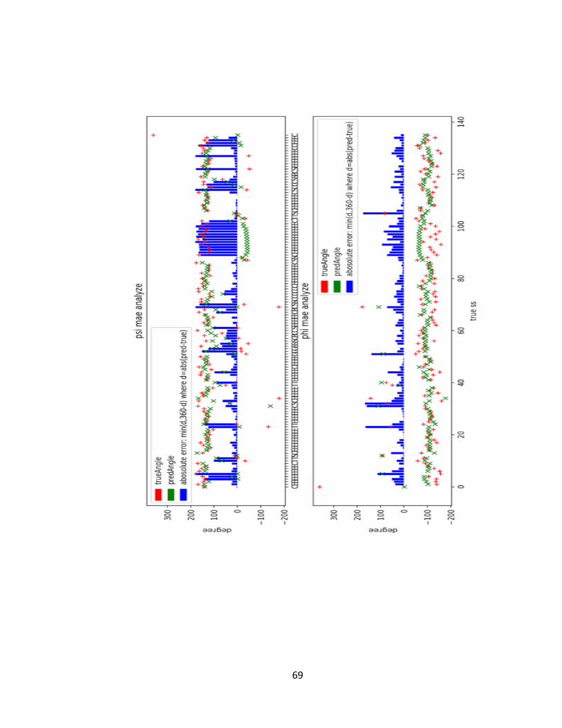
69

70
Figure 5-7 Psi-Phi angle prediction results of two proteins in CASP12, T0860 (top) and T0861 (bottom). Predicted angle value, true angle value, and absolute error are plotted for each amino acid position, which
is labelled by its true secondary structure type. The low blue bars, which denote the error between predicted angles and truth angels.
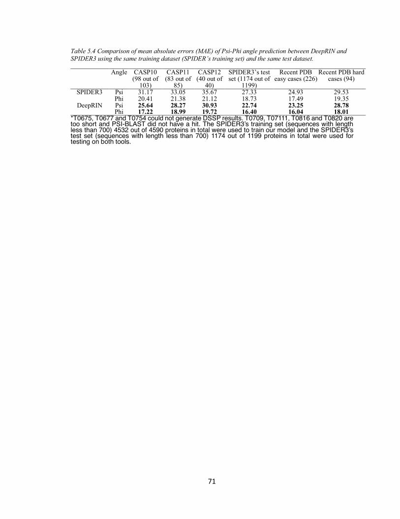
71
Table 5.4 Comparison of mean absolute errors (MAE) of Psi-Phi angle prediction between DeepRIN and SPIDER3 using the same training dataset (SPIDER’s training set) and the same test dataset.
Angle CASP10 (98 out of
103)
CASP11 (83 out of
85)
CASP12 (40 out of
40)
SPIDER3’s test set (1174 out of
1199)
Recent PDB easy cases (226)
Recent PDB hard cases (94)
SPIDER3 Psi 31.17 33.05 35.67 27.33 24.93 29.53 Phi 20.41 21.38 21.12 18.73 17.49 19.35
DeepRIN Psi 25.64 28.27 30.93 22.74 23.25 28.78 Phi 17.22 18.99 19.72 16.40 16.04 18.01
*T0675, T0677 and T0754 could not generate DSSP results. T0709, T07111, T0816 and T0820 are too short and PSI-BLAST did not have a hit. The SPIDER3’s training set (sequences with length less than 700) 4532 out of 4590 proteins in total were used to train our model and the SPIDER3’s test set (sequences with length less than 700) 1174 out of 1199 proteins in total were used for testing on both tools.

72
CHAPTER6 PROTEINBETATURNPREDICTIONUSING
DEEPDENSEINCETPIONNETWORKS
6.1 MethodsandMaterials
6.1.1 PreliminariesandProblemFormulation
To make an accurate prediction, it is important to provide useful input features to machine
learning models. In our method, we carefully designed feature matrices corresponding to
the primary amino acid sequence of a protein. Specifically, there are four features involved:
physicochemical feature, HHBlits profile, predicted eight state secondary structure from
MUFold-SS (Fang et al., 2018) and predicted shape string from Frag1D (Zhou et al., 2009).
The first set of features used is called physico-chemical features, which describe
hydrophobic, steric, and electric properties of amino acids and provide useful information
for protein sequence analysis and prediction. By using physico-chemical features, the
protein sequences are represented as an informative dense matrix. The physico-chemical
feature matrix consists of the sever physico-chemical properties as in (Heffernan et al.,
2017) plus a number 0 or 1 representing the existence of an amino acid at this position as
an input (called NoSeq label). The reason of adding the NoSeq label is because the
proposed deep neural networks are designed to take a fixed size input, such as a sequence
of length 700 residues in our experiment. To run a protein sequence shorter than 700
through the network, the protein sequence will be padded at the end with 0 values and the
NoSeq label is set to 1. If the protein is longer than 700 residues, it can be split into multiple
segments, each shorter than 700 residues. Hence, a protein sequence will be represented as
a 700-by-8 matrix, which is the first input feature for DeepDIN.
73
The second set of useful features comes from the protein profiles generated using
HHBlits (Remmert et al., 2012). In our experiments, the HHBlits software used the
database uniprot20_2013_03, which can be downloaded from
http://wwwuser.gwdg.de/~compbiol/data/hhsuite/databases/hhsuite_dbs/. The profile
values were transformed by the sigmoid function into the range (0, 1). Each amino acid in
the protein sequence is represented as a vector of 31 real numbers, of which 30 from amino
acids HHBlits profile values and 1 NoSeq label in the last column. The HHBlits, the names
of the parameters are amino acids and some transition probabilities: “A, C, D, E, F, G, H,
I, K, L, M, N, P, Q, R, S, T, V, W, Y, M->M, M->I, M->D, I->M, I->I, D->M, D->D, Neff,
Neff_I, and Neff_D”. HHBlits generates profiles which is more sensitive than PSI-BLAST
profile and provides useful evolutionary features for protein sequence. Hence, a HHBlits
profile will be represented as a 700-by-30 matrix, which is the second input feature for
DeepDIN.
The third set of useful features, predicted shape string, comes from Frag1D (Zhou et al.,
2009). For each protein sequence, the Frag1D can generate useful predicted protein 1D
structure features: the classical three-state secondary structure, three- and eight-state shape
string. Classical three state secondary structure contains H (helix), S (sheet), and R (random
loop). Eight state shape string label contains R (polyproline type alpha structure), S (beta
sheet), U, V (bridging regions), A (alpha helices), K (310 helices), G (almost entirely
glycine), and T (turns). The prediction of protein secondary structure has been used as an
important feature for protein structure prediction. However, for an average of 40% of all
residues in loop regions, the classical secondary structure does not carry useful structure
information. One the other hand, the protein structure can be described by pairs of psi phi

74
torsion angles. Ison et el. (2005) proposed Shape Strings, which can accurately describe a
1D string of symbols representing the protein backbone psi phi torsion angles. The shape
strings can describe the conformations of residues in regular secondary structure elements,
e.g. shape ‘A’ corresponds to alpha helix and shape ‘S’ corresponds to beta sheets. Besides,
shape strings classify the random loop regions into several states that can contain much
more conformation information, which is particularly useful for gamma-turn prediction
problem. For the Frag1D predicted result, each amino acid in the protein sequence is
represented as a vector of 15 numbers, of which 3 from the classical three-state secondary
structure, 3 from the three-state shape string, 8 from the eight-state shape string and 1
NoSeq label in the last column. The predicted classical three-state secondary structure
feature is represented as one-hot encoding as followed: helix: (1,0,0), strand: (0,1,0), and
loop: (0,0,1). The same rule applies to three- and eight-state shape string features. Hence,
a Frag1D result will be represented as a 700-by-15 matrix, which is the third input feature
for DeepDIN.
The fourth set of useful features comes from our previous designed secondary structure
prediction tool: MUFold-SS (Fang et al., 2018). MUFold-SS achieved state-of-the-art
performance in eight state secondary structure prediction and it should provide useful
features in beta-turn prediction tasks. The eight-state secondary structure are: H (alpha
helix), B (beta bridge), E (extended strand), G (3-helix), I (5 helix), T (hydrogen bonded
turn), and S (bend). Hence, an eight-state predicted secondary structure will be represented
as a 700-by-8 matrix, which is the fourth input feature for DeepDIN.

75
Protein beta-turn prediction is a classification problem. To be specific, it can be
formulated as residue-level prediction or turn-level prediction as first proposed by (Singh
et al., 2015).
Residue-level prediction: To predict each amino acid is a turn or non-turn. The class label
is either turn or non-turn. Here, the predicted output is a 700-by-3 matrix, where ‘700’ is
the sequence length 700 and ‘3’ stands for two-state labels plus 1 NoSeq label.
Turn-level prediction: At the turn-level, a sliding window of four residues was used to
generate the turn-level data sets. And the overall predicted beta-turn output of a protein
sequence is represented as a fixed-size matrix, with a (700-4+1) dimension by 3 for two-
state labels plus 1 NoSeq label matrix. For nine-class classification problem, the label is:
turn of the specific type or others.
The evaluation metric for beta-turn prediction typically uses MCC more often than
accuracy, since the accuracy only considers the true positive and false positive without the
true negative and false negative, and non-beta-turns (negative data) dominate the data.
MCC can be calculated as follows:
𝑀𝐶𝐶 =𝑇𝑃 ∗ 𝑇𝑁 − 𝐹𝑃 ∗ 𝐹𝑁
�(𝑇𝑃 + 𝐹𝑃)(𝑇𝑃 + 𝐹𝑁)(𝑇𝑁 + 𝐹𝑃)(𝑇𝑁 + 𝐹𝑁) 1)
where TP is the number of true positives, TN is the number of true negatives, FP is the
number of false positives and FN is the number of false negatives.
6.1.2 NewDeepDenseInceptionNetworksforProteinBeta-turnPrediction
(DeepDIN)
In this section, a new deep dense inception network architecture (DeepDIN) is presented.
The architecture makes use of deep inception (Szegedy et al., 2017) networks and dense

76
network (Huang et al., 2017). Figure 6-1 (A) presents our proposed network design. It
shows the beta-turn prediction:
1. Given a protein sequence, the system will generate four features: physico-chemical
feature, profile features from HHBlits, predicted shape string (using Frag1D) and
predicted eight-state secondary structure (using MUFold-SS).
2. The convolutional layer will then perform convolution operation on each feature to
get the coevolved feature map.
3. Concatenate four convolved feature maps along feature dimension.
4. Feed the concatenated feature map into stringed dense inception blocks (See Figure
2 (B) for illustration). In between there is a convolutional layer acting as transition
layer.
5. Predict beta-turn (either turn or non-turn) in the last dense layer which uses Softmax
as activation function.
Figure 6-1 (B) shows details of a dense inception block. It consists of four small version of
inception blocks and each inception block is fully connected with other inception blocks.
In other words, a dense inception module is constituted by connecting each inception layer
to every other inception layer in a feed-forward fashion. The design of dense inception
modules can extract non-local interactions of residues over a diverse range in a more
effective way. Adding more dense inception blocks is possible but requires more memory.
Each convolution layer, such as ‘Conv (3)’ in Figure 6-1, consists of four operations
sequentially: 1) A one-dimensional convolution operation using the kernel size of three; 2)
the Batch normalization technique (Ioffe and Szegedy, 2015) for speeding up the training
process and acting as a regularizer; 3) the activation operation, ReLU (Radford et al.,
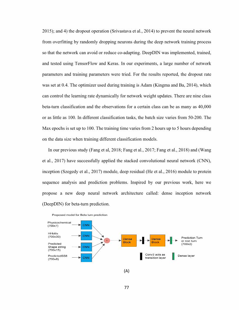
77
2015); and 4) the dropout operation (Srivastava et al., 2014) to prevent the neural network
from overfitting by randomly dropping neurons during the deep network training process
so that the network can avoid or reduce co-adapting. DeepDIN was implemented, trained,
and tested using TensorFlow and Keras. In our experiments, a large number of network
parameters and training parameters were tried. For the results reported, the dropout rate
was set at 0.4. The optimizer used during training is Adam (Kingma and Ba, 2014), which
can control the learning rate dynamically for network weight updates. There are nine class
beta-turn classification and the observations for a certain class can be as many as 40,000
or as little as 100. In different classification tasks, the batch size varies from 50-200. The
Max epochs is set up to 100. The training time varies from 2 hours up to 5 hours depending
on the data size when training different classification models.
In our previous study (Fang et al, 2018; Fang et al., 2017; Fang et al., 2018) and (Wang
et al., 2017) have successfully applied the stacked convolutional neural network (CNN),
inception (Szegedy et al., 2017) module, deep residual (He et al., 2016) module to protein
sequence analysis and prediction problems. Inspired by our previous work, here we
propose a new deep neural network architecture called: dense inception network
(DeepDIN) for beta-turn prediction.
(A)

78
(B)
Figure 6-1 (A) shows the overall proposed model for beta-turn prediction. (B) shows the details of a dense inception module that consists of four inception modules, each of which is fully connected in a feed forward
fashion.
6.1.3 ApplyTransferLearningandBalancedLearningtoDeepDINtoHandle
ImbalancedDataset
It is often unsuitable for tackling the problem of small sample sizes for deep learning. In
this work, in order to enable the deep neural networks to handle small classes, the following
deep learning strategies were used to address the small classes classification problem.
Balanced learning: Many previous researchers have studied the problem of imbalanced
data learning and proposed ways of balancing the data set by using either over-sampling
like SMOTE (Han et al., 2015) or under-sampling like Tomek Links (Tomek, 1976). The
beta-turn data is highly unbalanced, and this would cause the deep neural network like
DeepDIN prone to predict everything as the negative class. In this experiment, the protein
beta-turns as positive data are not very large, any up-sampling or down-sampling may
cause loss of useful information. Rather than re-sampling the training data points, a
balanced learning approach was adapted to handle the problem. The weighted cross entropy
was used as the loss function, which is defined as the following functions:

79
∀𝑖 ∈ [0,𝑁),𝐻(𝑖) = −�𝑦$,R ∗ 𝑙𝑜𝑔𝑦l$,R$
(2)
𝐻 =�𝑊 ∗ 𝑦$ ∗ 𝐻(𝑖)¡
(3)
where l is the number of classes; 𝑊 = (𝑤H, 𝑤(,… , 𝑤R) is the weight for each class; N is the
total number of data points; 𝑦$ is the one-hot ground truth label; 𝑦\g is the predicted
probability distribution of a data point; H(i) is the cross-entropy loss of one data; and H is
the weighted cross-entropy. The weighted cross entropy as the loss function was able to
address the issue caused by the small sample size by re-scaling the prediction of each class
by its weight. In this implementation, the class weights were calculated using training data
and assigned using the Scikit-learn (Pedregosa et al., 2011) toolbox. The balanced class
weights are given by 𝑛_𝑠𝑎𝑚𝑝𝑙𝑒𝑠/(𝑛_𝑐𝑙𝑎𝑠𝑠𝑒𝑠 ∗ 𝑏𝑖𝑛𝑐𝑜𝑢𝑛𝑡(𝑦)), where y is array of original
class labels per sample, “bincount” is a built-in function from Scikit-learn toolbox to
calculate the number of bins.
Transfer Learning: We applied transfer learning to handle the limited number of beta-
turn data used in the training set. The idea of transfer learning originally came from the
image classification problem (Raina et al., 2007). This technique was proposed to handle
the insufficient size of a data set that can be used to train the deep neural network. In our
study, since there are nine classes of beta-turns, and especially those in VIa1, VIa2, and
VIb contains a few hundred of data points, the amount of data belonging to each class may
not produce a model with the ability to extract features and being generalized well. To
solve this problem, the pre-trained weights from DeepDIN used to classify two-class beta-
turns was loaded into each separate nine-class classification model as initial weight. In

80
particular, the pre-trained model here is the beta-turn model used to classify the two-class
beta-turn problem. Since that model has “observed” some generic features of what a beta-
turn is, it should be useful to many specific nine-class beta-turn classification tasks. Then
for training each individual class model, the specific subset of the training set for each
individual class was fed into and the overall network weights were fine-tuned. The weights
of the pre-trained networks were fine-tuned by continuing the backpropagation. It is
possible to fix the earlier layer of the deep networks due to the overfitting issue and only
fine-tune the high-level portion of the network. After the trials, the overall network was
fine-tuned without freezing the lower level features.
For the learning rates during the transfer learning, a smaller learning rate (0.005) and
batch size (10) were used to train the network and fine-tune the network weights in the
fine-tuning. The reason is that the pre-trained network weights are relative good, a slower
and smaller learning rate will not distort them too quickly and too much before it converges.
6.1.4 Benchmarkdatasets
The following two publically available benchmark data sets were used in our experiments:
BT426 (Guruprasad and Rajkumar, 2000) is a data set commonly used for benchmarking
beta-turn prediction methods. BT426 contains 426 protein chains in total with 25
percentage sequence identity cutoffs, and resolution better than 2.0 Å. This benchmark was
used to compare the performance of many previous predictors, such as BetaTPred3 (Singh
et al., 2015) and NetTurnP (Petersen et al., 2010). In this work, five-fold cross-validation
experiments on BT426 were performed and results were compared against other predictors.

81
BT6376 (Singh et al., 2015) is a public benchmark containing 6376 non-homologous
protein chains. No two protein chains have more than 30% sequence identity. The
structures of these proteins were determined by X-ray crystallography at 2.0 Å resolution
or better. Each chain contains at least one beta-turn. The beta-turn labels were assigned by
PROMOTIF (Hutchinson and Thornton, 1996) program. This benchmark provides data
sets for both two-class beta-turn classification and nine-class beta-turn classification. For
the nine-class beta-turn labels were annotated by using PROMOTIF, too.
6.2 ResultsandDiscussion
In this section, extensive experimental results of the proposed deep neural networks on the
benchmark data sets and performance comparison with existing methods are presented. To
evaluate the performance of our tool, a five-fold cross validation technique was used on all
data sets.
6.2.1 HowFeatureAffectstheDeepDINPerformance
Since we used four features for our proposed DeepDIN architecture, it is important to
quantitatively determine how much improvement the proposed DeepDIN can make by
using single, some, or all of the features (See Table 6.2). We used TypeI beta-turns for
experiments. This dataset has 6039 proteins containing total of 42,393 TypeI beta-turns. In
each experiment, a five-fold cross-validation was performed. The running time for each
experiment is about 3-4 hours.
It can be found that the predicted shape string feature either used alone or used in
combined with other features can highly improve the prediction performance. However, it

82
suffers from high variance compared with other features. Using predicted shape string can
improve the prediction but the performance is not as stable as using other features.
Another observation is that some combined features have better prediction results than
those features used alone, which means features in-between can have some complementary
affect. For instance, when the predicted shape string is combined with the predicted
secondary structure as input, the prediction performance is much better than just using
predicted shape string. Although both features are related to protein secondary structure,
they may capture different aspect of features for a protein. Shape string combined with
secondary structure can achieve better results than shape string combined with
physicochemical feature.
From Table 6.1, it shows that if all four features were used, the prediction result is much
better and stable. We used all four features together in the other experiments.
Table 6.1 Different feature combinations will affect prediction performance
physicochemical SS8 Shape string HHBlits profile MCC
x 0.183(±0.013) x 0.311(±0.018) x 0.364(±0.058) x 0.321(±0.014)
x x 0.401(±0.002) x x 0.391(±0.052) x x 0.365(±0.011) x x 0.423(±0.031) x x 0.357(±0.014) x x 0.422(±0.042)
x x x 0.472(±0.040) x x x 0.454(±0.051) x x x 0.455(±0.037) x x x 0.446(±0.035)
x x x x 0.462(±0.027)

83
6.2.2 Residue-LevelandTurn-LevelTwo-ClassPredictiononBT426
Table 6.2 Residue-Level Prediction on BT426
Predictor MCC
BTPRED (Shepherd et al., 1999) 0.35 BetaTPred2 (Kaur and Raghava, 2002, 2004) 0.43
Hu and Li (2008) 0.47 NetTurnP (Petersen et al., 2010) 0.50
BetaTPred3-Tweak (Singh et al., 2015) 0.50 BetaTPred3-7Fold (Singh et al., 2015) 0.51
BetaTPred3 (Singh et al., 2015) 0.51 DeepDIN 0.647(±0.016)
Table 6.3 Turn-level Prediction on BT426
Features MCC
BetaTPred3 (Singh et al., 2015) 0.43
DeepDIN 0.550(±0.019)
Table 6.2 and 6.3 shows experiment results of comparing DeepDIN with existing
methods at residue-level and turn-level on benchmark BT426. At both residue-level or
turn-level, the DeepDIN outperformed all existing methods. In (Singh et al., 2015), they
proposed a “turn-level prediction formulation”, which predicts the complete beta-turn
rather than focusing on the residues in a beta-turn.
It is worth mentioning that in (Tang et al., 2011). They reported their turn-level MCC
around 0.66 on benchmark BT426. Actually, they preprocessed the dataset in a way that
the negative (non-turn) samples was randomly selected when the ratio of positive to
negative as 1:3 (Tang et al., 2011). In real world scenario, it is not possible to sample the
data this way. Our system can handle the original BT426 dataset (the ratio of positive to

84
negative as high as 1:9). Also, results comparison should be under same condition. In (Tang
et al., 2011), they compared their results using the preprocessed dataset with other
predictors using original BT426 dataset, which is not fair and objective comparison.
6.2.3 Turn-levelNine-ClassPredictiononBT6376
Table 6.4 show a list of class sizes information on the concrete sample and class sizes.
The purpose of this table is to give reader information on how small the positive turn
samples among all samples in each class. As one can see, for each beta-turn class, the
dataset is very imbalanced, as non-turn occupy majority of the data samples.
Table 6.5 shows the nine-class beta-turn prediction results. The average MCC results of
DeepDIN for large class beta-turns such as I, I’, II, II’, IV, outperformed BetaTPred3 at
least seven percentage points, which is a significant improvement. For some small classes
such as VIa1, VIb the improvement is about three percentage points. DeepDIN performs
not as good as BetaTPred3 in small classes such as VIa2 in average MCC, particularly
because of the small amount of training data points available. Generally speaking, deep
neural networks are always biased to predicted negative classes if a very small amount of
imbalanced observations are given. However, by applying balanced learning and transfer
learning, this issue can be alleviated or overcome.
Since the beta-turn dataset is very imbalanced, during training, different class weights
were calculated using the Scikit-learn (Pedregosa et al., 2011) toolbox and then assigned
to the loss function during the model training process. The experiments were performed on
an Alienware Area-51 desktop computer equipped with Nvidia Titan-X GPU (11 GB
memory). A five-fold cross-validation evaluation was performed on each of nine-class
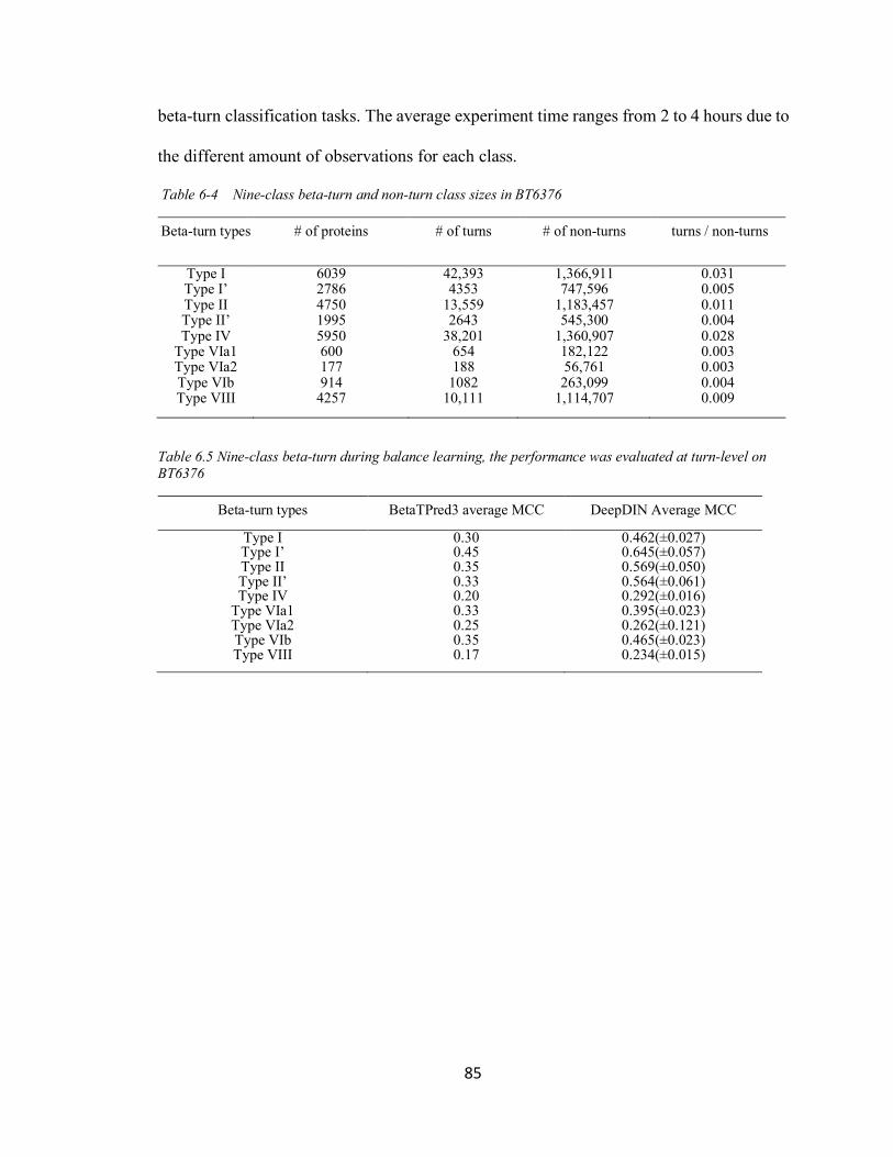
85
beta-turn classification tasks. The average experiment time ranges from 2 to 4 hours due to
the different amount of observations for each class.
Table 6-4 Nine-class beta-turn and non-turn class sizes in BT6376
Beta-turn types # of proteins # of turns # of non-turns turns / non-turns
Type I 6039 42,393 1,366,911 0.031 Type I’ 2786 4353 747,596 0.005 Type II 4750 13,559 1,183,457 0.011 Type II’ 1995 2643 545,300 0.004 Type IV 5950 38,201 1,360,907 0.028
Type VIa1 600 654 182,122 0.003 Type VIa2 177 188 56,761 0.003 Type VIb 914 1082 263,099 0.004 Type VIII 4257 10,111 1,114,707 0.009
Table 6.5 Nine-class beta-turn during balance learning, the performance was evaluated at turn-level on BT6376
Beta-turn types BetaTPred3 average MCC DeepDIN Average MCC
Type I 0.30 0.462(±0.027) Type I’ 0.45 0.645(±0.057) Type II 0.35 0.569(±0.050) Type II’ 0.33 0.564(±0.061) Type IV 0.20 0.292(±0.016)
Type VIa1 0.33 0.395(±0.023) Type VIa2 0.25 0.262(±0.121) Type VIb 0.35 0.465(±0.023) Type VIII 0.17 0.234(±0.015)

86
CHAPTER7 PROTEINGAMMATURNPREDICTIONUSING
DEEPDENSEINCETPIONNETWORKS
7.1 MaterialsandMethods
7.1.1 Problemformulation
A protein gamma-turn prediction is a binary classification problem, which can be
formulated as followed: given a primary sequence of a protein, a sliding window of k
residues were used to predict the central residue turn or non-turn. For example, if k is 17,
then each protein is subsequently sliced into fragments of 17 amino acids with a sliding
window.
To make accurate prediction, it is important to provide useful input features to machine-
learning methods. We carefully designed a feature matrix corresponding to the primary
amino acid sequence of a protein, which consists of a rich set of information derived from
individual amino acid, as well as the context of the protein sequence. Specifically, the
feature matrix is a composition of HHBlits profile (Remmert et al., 2012), and predicted
protein shape string using Frag1D (Zhou et al., 2009).
The first set of useful features comes from the protein profiles generated using HHBlits
(Remmert et al., 2012). In our experiments, the HHBlits software used database
uniprot20_2013_03, which can be downloaded from
http://wwwuser.gwdg.de/~compbiol/data/hhsuite/databases/hhsuite_dbs/. A HHBlits
profile can reflect the evolutionary information of the protein sequence based on a search
of the given protein sequence against a sequence database. The profile values were scaled

87
by the sigmoid function into the range (0, 1). Each amino acid in the protein sequence is
represented as a vector of 31 real numbers, of which 30 from HHM Profile values and 1
NoSeq label (representing a gap) in the last column. The HHBlits profile corresponds to
amino acids and some transition probabilities, i.e., A, C, D, E, F, G, H, I, K, L, M, N, P, Q,
R, S, T, V, W, Y, M->M, M->I, M->D, I->M, I->I, D->M, D->D, Neff, Neff_I, and
Neff_D.
The second set of useful features, predicted shape string, comes from Frag1D (Zhou et
al., 2009). For each protein sequence, Frag1D can generate useful predicted protein 1D
structure features: classical three-state secondary structures, and three- and eight-state
shape strings. Classical three-state secondary structures and three-state shape string labels
both contain H (helix), S (sheet), and R (random loop), but they are based on different
methods so that they have small differences. In this experiment, we used all the features
from Frag1D. Eight-state shape string labels contain R (polyproline type alpha structure),
S (beta sheet), U/V (bridging regions), A (alpha helices), K (310 helices), G (almost entirely
glycine), and T (turns). The classical prediction of three-state protein secondary structures
has been used as an important feature for protein structure prediction, but it does not carry
further structural information for the loop regions, which account for an average of 40% of
all residues in proteins. Ison et el. (2005) proposed Shape Strings, which give a 1D string
of symbols representing the distribution of protein backbone psi-phi torsion angles. The
shape strings include the conformations of residues in regular secondary structure
elements; in particular, shape ‘A’ corresponds to alpha helix and shape ‘S’ corresponds to
beta strand. Besides, shape strings classify the random loop regions into several states that
contain much more conformational information, which we found particularly useful for

88
gamma-turn prediction problem. For the Frag1D prediction result, each amino acid in the
protein sequence is represented as a vector of 15 numbers, of which 3 from the classical
three-state secondary structures, 3 from the three-state shape strings, 8 from the eight-state
shape strings and 1 NoSeq label in the last column. The predicted classical three-state
secondary structure feature is represented as one-hot encoding as followed: helix: (1,0,0),
strand: (0,1,0), and loop: (0,0,1). The same rule applies to three- and eight-state shape string
features. In this work, we also tried the traditional eight-state protein secondary structures.
However, the prediction result was not as good as the one from the eight-state shape strings.
This is probably because the traditional eight-state secondary structures contain much less
structural information for the gamma-turn prediction problem.
7.1.2 ModelDesign
In this section, a new deep inception capsule network (DeepICN) is presented. Figure
7-1 A shows the model design. The input features for DeepICN are HHBlits profiles and
predicted shape strings. Since the distributions of HHBlits profiles and predicted shape
strings are different, we applied convolutional filters separately on the two features, then
concatenated them. The CNN is used to generate the convolved features. We first applied
CNN to extract local low-level features from protein profiles and predicted shape strings
features. This CNN layer will extract local features similar to a CNN used to extract “edge”
features of objects in an image (Xie and Tu, 2015).
After the convoluted feature concatenation, the merged features are fed into the
inception module (See Figure 7-1 B for details). The inception network (Szegedy et al.,
2017) was then applied to extract low-to-intermediate features for CapsuleNet. In (Sabour

89
et al., 2017), CapsuleNet was used for digital image classification and the primary capsule
layers were placed after a convolutional layer. Their network design worked well for digital
image recognition with the image dimension 28-by-28. Considering the complex features
of protein HHblits profile and shape strings, it is reasonable to apply a deeper network to
extract local to medium level features so that CapsuleNet can work well on top of those
features and extract high-level features for gamma-turn classification. The purpose of
setting up an inception block right after CNN is to extract intermediate-level features.
(A)
(B)

90
(C)
Figure 7-1 (A) A deep inception capsule network design. The input features are HHBlits profile (17-by-30 2D array) and predicted shape string using Frag1D (17-by-15 2D array). Each feature is convolved by a convolutional layer. Both convolved features then get concatenated. An inception block is followed to extract low to medium features. A primary capsule layer then extracts higher level features. The final turn capsule layer makes predictions. (B) An inception block. Inside this inception block: Red square Conv(1) stands for convolution operation with kernel size 1. Green square Conv(3) stands for convolution operation with kernel size 3. Yellow square stands for feature map concatenation. (C) Zoom-in between primary capsules and turn capsules. The primary capsule layer contains 32 channels of convolutional 8D capsules. The final layer turn capsule has two 16D capsules to represent two states of the predicted label: gamma-turn or non-gamma-turn. The computation between those two layers is dynamic routing.
Each convolution layer, such as ‘Conv (3)’ in Figure 7-1 B, consists of four operations
in sequential order: (1) a one-dimensional convolution operation using the kernel size of
three; (2) the batch normalization technique (Ioffe and Szegedy, 2015) for speeding up the
training process and acting as a regularizer; (3) the activation operation, ReLU (Radford et
al., 2015); and (4) the dropout operation (Srivastava et al., 2014) to prevent the neural
network from overfitting by randomly dropping neurons during the deep network training
process so that the network can avoid co-adapting.
The capsule layers are placed after the inception module to extract high-level features
or explore the spatial relationship among the local features that are extracted in the above-

91
mentioned layers. The primary capsule layer (See Figure 7-1 C) is a convolutional capsule
layer as described in (Sabour et al., 2017). It contains 32 channels of convolutional 8D
capsules, with a 9 x 9 kernel and a stride of 2. The final layer (turn capsule) has two 16D
capsules to represent two states of the predicted label: gamma-turn or non-gamma-turn.
This layer receives the inputs from all the primary capsules output through the dynamic
routing algorithm (Sabour et al., 2017), which is an effective way to implement the
explaining away that is needed to segment highly overlapping objects (features). The
squashing activation function (Sabour et al., 2017) was applied in the computation between
the primary capsule layer and the turn capsule layer as follows:
𝑣? =V𝑠?V
1 + V𝑠?V(𝑠?V𝑠?V
where 𝑣? is the vector output of capsule j and 𝑠? is its total output.
The dynamic routing algorithm (Sabour et al., 2017) is as follows:
Routing Algorithm:
Routing (𝑢Z|\] , 𝑟, 𝑙)
For all capsule i in layer l and capsule j in layer (l+1):𝑏$,? ← 0
For r iteration do
For all capsule i in layer l:𝑐$ ← 𝑠𝑜𝑓𝑡𝑚𝑎𝑥(𝑏$)
For all capsule j in layer (𝑙 + 1): 𝒔𝒋 ← ∑ 𝑐$?𝒖g𝒋|𝒊$
For all capsule j in layer (𝑙 + 1): 𝒗𝒋 ← 𝑠𝑞𝑢𝑎𝑠ℎ(𝒔𝒋)
For all capsule i in layer l and capsule j in layer (𝑙 + 1):𝑏$? ← 𝑏$? + 𝑢l?|$ ∙ 𝒗𝒋

92
The evaluation matric for gamma-turn prediction more commonly uses Matthew
Correlation Coefficient (MCC) than percentage accuracy since the accuracy only considers
the true positives and false positives without the true negatives and false negatives. Another
reason is that the gamma-turn dataset is very imbalanced, where MCC can evaluate how
well the classifier performs on both positive and negative labels. MCC can be calculated
from the confusion matrix as follows:
𝑀𝐶𝐶 =𝑇𝑃 ∗ 𝑇𝑁 − 𝐹𝑃 ∗ 𝐹𝑁
�(𝑇𝑃 + 𝐹𝑃)(𝑇𝑃 + 𝐹𝑁)(𝑇𝑁 + 𝐹𝑃)(𝑇𝑁 + 𝐹𝑁)
where TP is the number of true positives, TN is the number of true negatives, FP is the
number of false positives and FN is the number of false negatives.
7.1.3 ModelTraining
DeepICN was implemented, trained, and tested using TensorFlow and Keras. Different
sets of hyper-parameters (dynamic routing iteration times, training data sample size,
convolution kernel size, and sliding window size) of DeepICN were explored. An early
stopping strategy was used when training the models and if the validation loss did not
reduce in 10 epochs, the training process stopped. The Adam optimizer was used to
dynamically change the learning rate during model training. All the experiments were
performed on an Alienware Area-51 desktop equipped with a Nvidia Titan X GPU (11 GB
graphic memory).
7.1.4 ExperimentDataset
1) CullPDB (Wang and Dunbrack, 2003) was download on November 2, 2017. It
originally contained 20,346 proteins with percentage cutoff 90% in sequence identity,

93
resolution cutoff 2.0 Å, and R-factor cutoff 0.25. This dataset was preprocessed and
cleaned up by satisfying all the following conditions: with length less than 700 amino acids;
with valid PSIBLAST profile, HHblits profile; with shape strings predicted by Frag1D
(Zhou et al., 2009); and with gamma-turn labels retrieved by PROMOTIF (Hutchinson and
Thornton, 1996). After this, 19,561 proteins remained and CD-Hit (Li and Godzik, 2006)
with 30% sequence identity cutoff was applied on this dataset resulting in 10,007 proteins.
We removed proteins with sequence identity more than 30% for an objective and strict test
in terms of model generalization. This dataset was mainly used for deep neural network
hyper-parameter tuning and the exploration of CapsuleNet configurations. It was also used
to compare the proposed inception capsule model with other deep-learning models. For
these purposes, a balanced dataset was built: all positive gamma-turn labels and an equal
size of negative non-gamma-turn labels were selected to form a balanced dataset.
2) The benchmark GT320 (Guruprasad and Rajkumar, 2000) is a common data set used
for benchmarking gamma-turn prediction methods. GT320 contains 320 non-homologous
protein chains in total with 25% sequence identity cutoffs, and resolution better than 2.0 Å
resolution. This benchmark was used to compare the performance with previous predictors.
Each chain contains at least one gamma-turn. The gamma-turns were assigned by
PROMOTIF (Hutchinson and Thornton, 1996). In this work, five-fold cross-validation
experiments on GT320 was performed and results were compared against other predictors.

94
7.2 ExperimentalResults
In this section, extensive experimental results of the proposed deep CapsuleNets with
different hyper-parameters were tuned and tested using CullPDB and five-fold cross-
validation results on GT320. The performance comparison with existing methods is
presented.
7.2.1 Hyper-parameter Tuning and Model Performance
Tables 7.1-4 show the exploration of the inception capsule network with different
hyper-parameters. This set of experiments was to find out a better configuration of hyper-
parameters for the deep networks using the CullPDB dataset. Since this network involves
many hyper-parameters, only the major ones were explored. Table 1 shows how the sliding
window size affects the model performance. In this experiment, 1000 proteins were
randomly selected to form the training set, 500 for the validation set and 500 for the test
set. Each experiment was performed with five times of data randomization.
Table 7.1 shows how the sliding window size of input affects the deep capsule network
performance. The larger the window size, the more training time it took for CapsuleNet.
However, MCC may not grow as the window size increases. We chose the window size of
17 amino acids based on its peak MCC performance in the experiments. The t-test p-values
show that the window size 17 test MCC compared to other window sizes is statistically
significant.
Table 7.2 shows the dropout rate’s effects on the performance of the deep capsule
network. If a dropout was not used, the network had very high over-fitting. The dropout
rate 0.4-0.5 is reasonable as it is a compromise between the training and test prediction
performance. We chose dropout 0.5 in our study. The P-value between the dropout of 0.5

95
and any of others was insignificant. Although The dropout of 0.8 had the highest test
average MCC, its standard deviation (±0.0249) is also high, and hence, we did not use it.
Table 7.1 Effect of window size on MCC performance
Window size Test average MCC Time (hr) P-value on MCC
15 0.4458(±0.0107) 0.18(±0.11) 0.0115 17 0.4645(±0.0062) 0.24(±0.15) - 19 0.4442(±0.0049) 0.37(±0.18) 0.0010 21 0.4548(±0.0055) 0.43(±0.20) 0.0499 23 0.4227(±0.0076) 0.37(±0.23) 0.0001 25 0.4369(±0.0076) 0.45(±0.25) 0.0005
Table 7.2 Effect of dropout on MCC performance
Dropout Train average MCC Test average MCC P-value on test MCC
No 0.9974(±0.0015) 0.4439(±0.0101) 0.1236 0.3 0.9857(±0.0154) 0.4454(±0.0049) 0.0843 0.4 0.9010(±0.1457) 0.4515(±0.0047) 0.4294 0.5 0.9377(±0.0598) 0.4558(±0.0092) - 0.6 0.9159(±0.0688) 0.4525(±0.0111) 0.6647 0.7 0.8371(±0.0920) 0.4604(±0.0063) 0.4318 0.8 0.6072(±0.1033) 0.4646(±0.0249) 0.5228
Table 7.3 Effect of training size on training time and MCC performance
Training size Test average MCC Time (hr)
500 0.4224(±0.0035) 0.23(±0.17) 1000 0.4553(±0.0098) 0.87(±0.03) 2000 0.4422(±0.0204) 1.59(±0.07) 3000 0.4752(±0.0111) 2.38(±0.09) 4000 0.4787(±0.0147) 3.13(±0.12) 5000 0.4717(±0.0165) 3.91(±0.14)
Table 7.4 Effect of dynamic routing on MCC performance
dynamic routing times
Test average MCC Time (hr) P-value on MCC
1 0.4454(±0.0049) 0.44(±0.16) 0.4644 2 0.4492(±0.0086) 0.31(±0.17) - 3 0.4407(±0.0032) 0.37(±0.15) 0.1017 4 0.4497(±0.0045) 0.32(±0.18) 0.9276 5 0.4487(±0.0061) 0.41(±0.14) 0.9502

96
Table 7.3 shows the effects of the training sample size on the deep capsule network
training speed and performance. More training data increased and training time and the
model performance. However, after 3000 samples, the MCC performance did not improve
significantly with more training data. This is consistent with the observation in (Sabour et
al., 2017) that CapsuleNet did not need a large dataset for training.
Table 7.4 shows the effect of number of dynamic routing on the performance. Dynamic
routing is used in CapsuleNet similar to max-pooling in a CNN, but it is more effective
than max-pooling in that it allows neurons in one layer to ignore all but the most active
feature detector in a local pool in the previous layer. In this experiment, we fixed the other
hyper-parameters searched in the above-mentioned experiments and studied how number
of dynamic routing affected the performance. Considering the training time and the MCC
performance, 2 routings are suitable, as more dynamic routing does not have significant
improvement. The training time did not show large variations as the number of dynamic
routings increases. This may be because our experiments used early stopping.
7.2.2 Prediction confidence: the capsule length
According to (Sabour et al., 2017), the capsule length indicates the probability that the
entity represented by the capsule is present in the current input. In other words, the capsule
length in the last layer can be used for prediction of gamma-turn and assessment of
prediction confidence. The longer the turn capsule length is, the more confident the
prediction of a turn capsule will be. Here, the capsule length in Turn Capsules can be used
to show how confidence a gamma-turn is predicted. Specifically, a test set (with 5000
proteins containing 19,594 data samples) was fed into the trained inception capsule
network to get a capsule length vector. Then the capsule length vector that represents

97
positive capsules were kept. Since all the capsule length values fall into the range between
0 and 1, they were grouped into bins with the width of 0.05, so that there are totally 20
bins. The precision of each bin can be calculated to represent the prediction confidence.
Figure 7-2 shows the fitting curve of precision (percentage of correctly predicted gamma-
turns, i.e., true positives in the bin) versus the capsule length. A nonlinear regression curve
was used to fit all the points, yielding the following equation:
𝑦 = 1.084𝑥( − 0.203𝑥 + 0.147
where x is the capsule length and y is the precision.
The fitting-curve can be further used for prediction confidence assessment: given a
capsule length, its prediction confidence can be estimated using the above equation.
Figure 7-2 The fitting curve of precision (percentage of true positive in the bin) versus the capsule length. The green line is the fitting curve and the blue line (y=x^2) is for reference.

98
7.2.3 Proposed model performance compared with previous predictors
For comparing with other predictors, the public benchmark GT320 was used. Following
the previous studies, a five-fold cross validation results were reported, as shown in Table
7.5. This GT320 is an imbalanced dataset, but for objective evaluation, we did not sample
any balanced data from training or testing, as done in previous studies. Table 7.5 shows
that the proposed inception capsule network outperformed all the previous methods by a
significant margin.
Table 7.5 Performance comparison with previous predictors using GT320 benchmark.
Methods MCC
Our Approach 0.45 Zhu et al., 2012 0.38
Hu’s SVM 0.18 SNNS 0.17
GTSVM 0.12 WEKA-logistic regression 0.12
WEKA-naïve Bayes 0.11
*The results of WAKA, SNNS were obtained from (Kaur and Raghava, 2002), the result of GTSVM was obtained from (Pham et al., 2005) and result of Hu’s SVM was from (Hu and Li, 2008). Zhu et al., (2012) is the previous best predictor result. 7.2.4 Extend CapsuleNet for classic and inverse gamma-turn prediction
Many previous gamma-turn predictors only predict whether a turn is gamma-turn or not.
Here, we also extended our deep inception capsule model for classic and inverse gamma-
turn prediction. The experiment dataset is still CullPDB, and inverse and classic labels
were assigned using PROMOTIF (Hutchinson and Thornton, 1996). The same deep
inception capsule network (shown in Figure 7-1 A) was applied except the last turn capsule
layer now has three capsules to predict non-turn, inverse turn or classic turn as a three-class
classification problem. The performance metric Q3 is used which is the accuracy of correct
prediction for each class. The prediction results are shown in Table 6. Different numbers
of proteins were used to build the training set. The validation and test set contain 500

99
proteins each. The CullPDB dataset contains 10,007 proteins which have 1383 classic
turns, 17,800 inverse turns, and 2,439,018 non-turns in total. This is a very imbalanced
dataset. In this experiment, the balanced training set, validation set, and test set were
generated as follows: The inverse turn samples were randomly drawn as much as classic
turn sample size. For the non-turn samples, they were randomly drawn twice as much as
classic turn sample size, i.e. the sum of inverse turn samples and classic turn samples. The
training loss and validation loss curves are shown in Figure 7-3. From the loss curve, it
shows that after about 75 epochs, the model learning process was converging. Since the
model hyper-parameters had been explored in the earlier experiments, during this
experiment, we adopted similar values, i.e., the window size was chosen 17 amino acids,
the filter size is 256, the convolution kernel size was chosen 3, the dynamic routing was
chosen 3 iterations and dropout ratio was 0.3.
Figure 7-3 Training loss and validation loss curve of deep inception capsule network for classic and inverse gamma-turn.

100
Table 7.6 Non-turn, inverse and classic turn prediction results.
Training size Test average Q3 Time (hr) P-value
5000 0.6839(±0.0053) 0.25(±0.20) - 6000 0.6783(±0.0076) 0.38(±0.22) 0.2706 7000 0.6864(±0.0124) 0.34(±0.16) 0.3057
7.2.5 Visualization of the features learnt by capsules
In order to verify whether the extract high-level features learnt/extracted from the input
data have the prediction power and are generalizable, t-SNE (Maaten and Hinton, 2008)
was applied to visualize the input features and the capsule features for both the training
data and the test data. Figure 7-4 (A) shows the t-SNE plot of the input features from the
training data before the training. The input data has 45 features (i.e. 45 dimensions), and t-
SNE can project 45 dimensions onto two principal dimensions and visualize it. There was
no clear cluster in the training data. Figure 7-4 (B) shows the t-SNE plot of the capsule
features from the training data. The turn capsule contains 16 dimensions, and the t-SNE
can similarly project the capsule features to two major principal features and visualize it.
The clusters were obviously formed after the training. Figure 7-4 (C) and (D) show the t-
SNE plots for the input features and the capsule features of the test data. There was no clear
cluster for the input features in the test data either. The capsule features still tend to be
clustered together in the test data, although to less extent than the training data.

101
(A)
(B)

102
(C)
(D)

103
Figure 7-4 t-SNE plots of capsule network features. (A) and (B) are plots of the input features and the capsule features, respectively for training dataset (3000 proteins with 1516 turn samples). (C) and (D) are plots of the input features and the capsule features, respectively for the test dataset (500 proteins with 312 turn samples). Red dots represent non-turns, green dots represent inverse turns and blue dots represent classic turns.
Figure 7-5 (A) shows the classic turn Weblogo and Figure 7-5 (B) shows the inverse
turn Weblogo (Crooks et al., 2004). In the two plots, the y axis has the same height of 0.8
bits. Both types of turns have some visible features and the classic turn Weblogo contains
more information content than the inverse turn.
(A)
(B)

104
(C)
Figure 7-5 (A) Classic turn Weblogo; (B) inverse turn Weblogo; and (C) Non-turn Weblogo
7.2.6 Ablation study
To discovery the important elements in our proposed network, an ablation study was
performed by removing or replacing different components in the deep inception capsule
network. In particular, we tested the performance of the proposed models without the
capsule component, replacing the capsule component with CNN, or replacing inception
component with CNN. These sets of experiments were performed using the same amount
of data (3000 proteins for training, 500 proteins for validation, and 500 for test) and the
same parameter setting: dropout ratio 0.5 and window size 17. From the ablation test result
presented in Table 7.7, we found that the capsule component is the most effective
component in our network, since the performance dropped significantly when removing or
replacing the capsule component. The inception component also acts as an important
component as it can effectively extract feature maps for capsule components compared to
CNN.

105
Table 7.7 Ablation test.
Model MCC
Replace inception component with CNN 0.4544(±0.0106) Replace capsule component with CNN 0.4485(±0.0056)
Without capsule component 0.4551(±0.0059) Proposed Design 0.4752(±0.0111)
7.3 ConclusionandDiscussion
In this work, the latest deep-learning framework, CapsuleNet, was applied to protein
gamma-turn prediction. Instead of applying capsule network directly, a new model called
inception capsule network was proposed and has shown improved performance comparing
to previous predictors. This work has several innovations.
First of all, this work is the first application of deep neural networks to protein gamma-
turn prediction. Compared to previous traditional machine-learning methods for protein
gamma-turn prediction, this work uses a more sophisticated, yet efficient, deep-learning
architecture, which outperforms previous methods. A software tool has been developed
and it will provide the research community a powerful deep-learning prediction tool for
gamma-turn prediction. The ablation test was performed, and the importance of capsule
component was verified.
Second, this work is the earliest application of CapsuleNet to protein structure-related
prediction, and possibly to any bioinformatics problems to our knowledge, as CapsuleNet
was just published in 2017. Here, we proposed an inception capsule network for protein
gamma-turn prediction and explored some unique characters of capsules. To explore the
capsule length, we designed an experiment of grouping each capsule length into several
bins and discovered the relationship between prediction precision and capsule length. A

106
nonlinear curve can be applied to fit the data and further used for estimating the prediction
confidence. In addition, the network was extended to inverse turn and classical turn
prediction. The inverse turn capsule and classical turn capsule were further explored by
showing the t-SNE visualization of the learnt capsule features. Some interesting motifs
were visualized by Weblogo.
Third, new features have been explored and applied to gamma-turn prediction. The
features used for network training, namely HHBlits profiles and predicted shape string,
contain high information content making deep learning very effective. The HHBlits
profiles provide evolutionary information while shape strings provide complementary
structural information for effectively predicting gamma turns.
Last but not least, previous gamma-turn resources are very limited and outdated. A few
servers are not maintained, and no downloadable executable of gamma-turn is available.
Here a free tool with source code utilizing deep learning and state-of-the-art CapsuleNet
will be ready for researchers to use.

107
CHAPTER8 SUMMARY
Protein secondary structure and super-secondary structure are providing useful features
for protein tertiary structure prediction. Deep learning can lead to significant improvement
to these problems. In this dissertation, several novel deep neural networks were proposed
for protein secondary structure and super-secondary structure prediction:
In the work of Deep Inception-Inside-Inception, a new deep neural network architecture
Deep3I was proposed for protein secondary structure prediction and other protein structural
feature prediction, such as Psi-Phi angle prediction. Extensive experimental results show
that Deep3I obtained more accurate predictions than the best state-of-the-art methods and
tools. The experiments were designed carefully, and the datasets used in training, e.g., the
CullPDB dataset, were processed to remove any significantly similar sequences with the
test sets using CD-HIT to avoid any bias. Compared to previous deep-learning methods for
protein secondary structure prediction and Psi-Phi angle prediction, this work uses a more
sophisticated, yet efficient, deep-learning architecture. Deep3I utilizes hierarchical deep
Inception blocks to effectively process local and non-local interactions of residues. An
open source software has been developed based on Deep3I. It will provide the research
community a powerful prediction tool for secondary structures and Psi-Phi angles. A URL
for downloading the tool will be provided upon acceptance of publication.
In the work of Deep neighbor residual network: Compared with previous deep-learning
methods for protein secondary structure prediction, the new method consists of two types
of networks: a new deep neighbor residual network (DeepNRN) for predicting secondary
structures and a Struct2Struct network for making the predictions more protein-like.

108
Extensive experimental results show the new method achieved better Q3 and Q8 prediction
accuracies than existing state-of-the-art methods.
In the work of deep residual inception network, a new deep neural network architecture
DeepRIN was proposed for protein Psi-Phi angle prediction. Extensive experimental
results show that DeepRIN consistently generated more accurate predictions than the best
state-of-the-art methods. The experiments were designed carefully, and the datasets used
in training, e.g., the CullPDB dataset, were processed to remove any significantly similar
sequences with the test sets using CD-HIT to avoid any bias. Compared to previous deep-
learning methods for Psi-Phi angle prediction, this work developed a more sophisticated,
yet efficient, deep-learning architecture. DeepRIN utilized hierarchical deep Inception
blocks to effectively process local and non-local interactions between residues and the
residual shortcuts help propagate high-level features into deep networks. A software tool
has been developed based on DeepRIN and is made available to the research community
for download at http://dslsrv8.cs.missouri.edu/~cf797/MUFoldAngle/.
In the work of deep dense inception network, a new a new deep neural network
architecture DeepDIN was proposed for protein beta-turn prediction. Extensive
experimental results show that DeepDIN obtained more accurate predictions than the best
state-of-the-art methods and tools. Compared to previous machine-learning methods for
protein beta-turn prediction, this work uses a more sophisticated, yet efficient, deep-
learning architecture. The proposed DeepDIN takes input of the entire protein sequence as
the input feature, whereas all previous predictors rely on a fix-sized sliding window, which
is more effective and efficient to extract long-range residue interactions. DeepDIN utilizes
densely connected inception blocks to effectively process local and non-local interactions

109
of residues. Second, since the beta-turn dataset is very imbalanced (the ratio of positive
samples over negative samples is about 1:9). balanced learning and transfer learning were
applied overcome the problem. It is worth mentioning that the transfer learning was
originally applied to image recognition tasks, here we apply similar method to training
models for small beta-turn classification tasks. The pre-trained base network is effective in
learning some more general beta-turn features, then the transfer learning technique can
transfer the base network to some more specific models that can classifying nine-class beta-
turns. This demonstrate some goods example of handling imbalance dataset in protein
sequence analysis. Third, this work quantitatively discovered how different input features
can affect the beta-turn prediction. For example, some good features such as shape string
and HHBlits profile can improve beta-turn classification effectively. In the future work,
the small beta-turn classes still have room for further improvement. Also, those features
can be useful for other turn prediction problems, such as gamma-turn prediction (Pham et
al., 2005). Last but not least, we have implemented a tool called MUFold-BetaTurn which
utilizing the proposed DeepDIN achitecture for beta-turn prediction. This tool is ready for
research community to use freely.
In this work of deep inception capsule network, the latest deep-learning framework,
CapsuleNet, was applied to protein gamma-turn prediction. Instead of applying capsule
network directly, a new model called inception capsule network was proposed and has
shown improved performance comparing to previous predictors. This work has several
innovations. First of all, this work is the first application of deep neural networks to protein
gamma-turn prediction. Compared to previous traditional machine-learning methods for
protein gamma-turn prediction, this work uses a more sophisticated, yet efficient, deep-

110
learning architecture, which outperforms previous methods. A software tool has been
developed and it will provide the research community a powerful deep-learning prediction
tool for gamma-turn prediction. The ablation test was performed, and the importance of
capsule component was verified. Second, this work is the earliest application of
CapsuleNet to protein structure-related prediction, and possibly to any bioinformatics
problems to our knowledge, as CapsuleNet was just published in 2017. Here, we proposed
an inception capsule network for protein gamma-turn prediction and explored some unique
characters of capsules. To explore the capsule length, we designed an experiment of
grouping each capsule length into several bins and discovered the relationship between
prediction precision and capsule length. A nonlinear curve can be applied to fit the data
and further used for estimating the prediction confidence. In addition, the network was
extended to inverse turn and classical turn prediction. The inverse turn capsule and classical
turn capsule were further explored by showing the t-SNE visualization of the learnt capsule
features. Some interesting motifs were visualized by Weblogo. Third, new features have
been explored and applied to gamma-turn prediction. The features used for network
training, namely HHBlits profiles and predicted shape string, contain high information
content making deep learning very effective. The HHBlits profiles provide evolutionary
information while shape strings provide complementary structural information for
effectively predicting gamma turns. Last but not least, previous gamma-turn resources are
very limited and outdated. A few servers are not maintained, and no downloadable
executable of gamma-turn is available. Here a free tool with source code utilizing deep
learning and state-of-the-art CapsuleNet will be ready for researchers to use.

111
Last but not least, we built a web server called MUFold-SS-Angle that predicts protein
secondary structure and backbone torsion angle from the protein sequence. This server
employs MUFold-SS and MUFold-Angle, which are two standalone tools we recently
developed to predict secondary structure and backbone torsion angles, respectively. Both
tools outperform other predictors/servers in both easy cases (proteins with similar
sequences in PDB) or hard cases (proteins without detectable similarity in PDB) on
extensive test cases.
The major achievements and contributions are:
1) A new very deep learning network architecture, Deep3I, was proposed to effectively
process both local and global interactions between amino acids in making accurate
secondary structure prediction and Psi-Phi angle prediction. Extensive experimental
results show that the new method outperforms the best existing methods and other deep
neural networks significantly. An open-source tool Deep3I-SS was implemented based
on the new method. This tool can predict the protein secondary structure and the Psi-
Phi angles fast and accurately.
2) DeepNRN, a new deep-learning network with new architecture, is proposed for protein
secondary structure prediction; and experimental results on the CB513, CASP10,
CASP11, CASP12 benchmark data sets show that DeepNRN outperforms existing
methods and obtains the best results on multiple data sets.
3) A new deep neural network architecture, DeepRIN, is proposed to effectively capture
and process both local and global interactions between amino acids in a protein
sequence. Extensive experiments using popular benchmark datasets were conducted to
demonstrate that DeepRIN outperformed the best existing tools significantly. A
112
software tool based on DeepRIN is made available to the research community for
download.
4) A new deep neural network architecture, DeepDIN, is proposed to beta-turn
classification problem. In addition, balanced learning and transfer learning techniques
were applied overcome the problem of imbalanced dataset. Several new features were
explored quantitatively for beta turn prediction effectively.
5) A new deep neural network architecture, DeepICN, is proposed to gamma-turn
classification problem. Also, capsule length, representing the confidence of prediction,
was further explored. This is the first application of capsule networks to biological
sequence analysis.
6) A new web server, called MUFold-SS-Angle, is a combined web service of both
MUFold-SS and MUFold-Angle tools and will provide the community a better usage
of the software.

113
Refereed publication:
• Fang, Chao, Yi Shang, and Dong Xu. “A New Deep Neighbor-Residual Neural
Network for Protein Secondary Structure Prediction.” Tools with Artificial
Intelligence (ICTAI), 2017 IEEE 29th International Conference on. IEEE, 2017.
• Fang, Chao, Yi Shang, and Dong Xu. "MUFOLD-SS: New deep inception-inside-
inception networks for protein secondary structure prediction." Proteins: Structure,
Function, and Bioinformatics 86.5 (2018): 592-598.
• Fang, Chao, Yi Shang, and Dong Xu. "Prediction of Protein Backbone Torsion Angles
Using Deep Residual Inception Neural Networks." IEEE/ACM Transactions on
Computational Biology and Bioinformatics (2018).
• Fang, Chao, Yi Shang, and Dong Xu. (2018). “Improving Protein Gamma-Turn
Prediction Using Inception Capsule Networks.” (submitted)
• Fang, Chao, Yi Shang, and Dong Xu. (2018). “MUFold-BetaTurn: A Deep Inception
Network for Protein Beta-Turn Prediction” (submitted)
• Fang, Chao, Zhaoyu Li, Dong Xu and Yi Shang. (2018) “MUFold-SS-Angle: A Web
Server for Protein Secondary Structure and Backbone Torsion Angle Prediction.”
Bioinformatics, (submitted).

114
REFERENCE
Abadi, M., Agarwal, A., Barham, P., Brevdo, E., Chen, Z., Citro, C., Corrado, G.S., Davis,
A., Dean, J., Devin, M. and Ghemawat, S., (2016). Tensorflow: Large-scale machine
learning on heterogeneous distributed systems. arXiv preprint arXiv:1603.04467.
Adamczak, R., Porollo, A. and Meller, J., (2004). Accurate prediction of solvent
accessibility using neural networks–based regression. Proteins: Structure, Function,
and Bioinformatics, 56(4), pp.753-767.
Altschul, S.F., Madden, T.L., Schäffer, A.A., Zhang, J., Zhang, Z., Miller, W. and Lipman,
D.J., (1997). Gapped BLAST and PSI-BLAST: a new generation of protein database
search programs. Nucleic acids research, 25(17), pp.3389-3402.
Alkorta, I., Suarez, M. L., Herranz, R., González-Muñiz, R., and García-López, M. T.
(1996). Similarity study on peptide γ-turn conformation mimetics. Molecular modeling
annual, 2(1), 16-25.
Anfinsen, C. B. (1973). Principles that govern the folding of protein
chains. Science, 181(4096), 223-230.
Asgari, E. and Mofrad, M.R., (2015). Continuous distributed representation of biological
sequences for deep proteomics and genomics. PloS one, 10(11), p.e0141287.
Bahdanau, D., Cho, K., and Bengio, Y. (2014). Neural machine translation by jointly
learning to align and translate. arXiv preprint arXiv:1409.0473.
Berman, H. M., Westbrook, J., Feng, Z., Gilliland, G., Bhat, T. N., Weissig, H., ... &
Bourne, P. E. (2006). The Protein Data Bank, 1999–. In International Tables for
Crystallography Volume F: Crystallography of biological macromolecules (pp. 675-
684). Springer Netherlands.

115
Biegert, A. and Söding, J., (2009). Sequence context-specific profiles for homology
searching. Proceedings of the National Academy of Sciences, 106(10), pp.3770-3775.
Bjorkman, P. J., & Parham, P. (1990). Structure, function, and diversity of class I major
histocompatibility complex molecules. Annual review of biochemistry, 59(1), 253-288.
Boratyn, G.M., Schäffer, A.A., Agarwala, R., Altschul, S.F., Lipman, D.J. and Madden,
T.L., (2012). Domain enhanced lookup time accelerated BLAST. Biology direct, 7(1),
p.12.
Bragg, W. L., Phillips, D. C., & Lipson, H. (1975). development of X-ray analysis. G. Bell.
Busia, A. and Jaitly, N., (2017). Next-Step Conditioned Deep Convolutional Neural
Networks Improve Protein Secondary Structure Prediction. arXiv preprint
arXiv:1702.03865.
Bystrov, V. F., Portnova, S. L., Tsetlin, V. I., Ivanov, V. T., and Ovchinnikov, Y. A. (1969).
Conformational studies of peptide systems: The rotational states of the NH-CH
fragment of alanine dipeptides by nuclear magnetic resonance. Tetrahedron, 25(3),
493-515.
Cheng, J., Randall, A.Z., Sweredoski, M.J. and Baldi, P., (2005). SCRATCH: a protein
structure and structural feature prediction server. Nucleic acids research, 33(Suppl. 2),
pp.W72-W76.
Chollet, F., (2015). Keras.
Chollet, F. (2016). Xception: Deep Learning with Depthwise Separable
Convolutions. arXiv preprint arXiv:1610.02357.

116
Ciregan, D., Meier, U., & Schmidhuber, J. (2012, June). Multi-column deep neural
networks for image classification. In Computer Vision and Pattern Recognition
(CVPR), 2012 IEEE Conference on (pp. 3642-3649). IEEE.
Collobert, R., & Weston, J. (2008, July). A unified architecture for natural language
processing: Deep neural networks with multitask learning. In Proceedings of the 25th
international conference on Machine learning (pp. 160-167). ACM.
Chou, P. Y., and Fasman, G. D. (1979). Prediction of beta-turns. Biophysical
Journal, 26(3), 367-383.
Chou, K. C., and Blinn, J. R. (1997). Classification and prediction of β-turn types. Journal
of protein chemistry, 16(6), 575-595.
Chou, P. Y., and Fasman, G. D. (1974). Conformational parameters for amino acids in
helical, β-sheet, and random coil regions calculated from proteins. Biochemistry, 13(2),
211-222.
Chou, K. C. (1997). Prediction of beta-turns in proteins. J Pept Res, 49(2), 120-44.
Cole, C., Barber, J. D., and Barton, G. J. (2008). The Jpred 3 secondary structure prediction
server. Nucleic acids research, 36(suppl_2), W197-W201.
Crooks, G. E., Hon, G., Chandonia, J. M., and Brenner, S. E. (2004). WebLogo: a sequence
logo generator. Genome research, 14(6), 1188-1190.
Dai, L. and Zhou, Y., 2011. Characterizing the existing and potential structural space of
proteins by large-scale multiple loop permutations. Journal of molecular
biology, 408(3), pp.585-595.

117
Deng, J., Dong, W., Socher, R., Li, L. J., Li, K., & Fei-Fei, L. (2009, June). Imagenet: A
large-scale hierarchical image database. In Computer Vision and Pattern Recognition,
2009. CVPR 2009. IEEE Conference on (pp. 248-255). IEEE.
Dill, K. A. (1990). Dominant forces in protein folding. Biochemistry, 29(31), 7133-7155.
Dill, K. A., & MacCallum, J. L. (2012). The protein-folding problem, 50 years
on. science, 338(6110), 1042-1046.
Dor, O., & Zhou, Y. (2007). Achieving 80% ten-fold cross-validated accuracy for
secondary structure prediction by large-scale training. Proteins: Structure, Function,
and Bioinformatics, 66(4), 838-845.
Dor, O., & Zhou, Y. (2007). Real-SPINE: An integrated system of neural networks for real-
value prediction of protein structural properties. PROTEINS: Structure, Function, and
Bioinformatics, 68(1), 76-81.
Drozdetskiy, A., Cole, C., Procter, J. and Barton, G.J., (2015). JPred4: a protein secondary
structure prediction server. Nucleic acids research, 43(W1), pp.W389-W394.
Fang, C., Shang, Y., and Xu, D. (2018). MUFOLD-SS: New Deep Inception-Inside-
Inception Networks for Protein Secondary Structure Prediction. Proteins: Structure,
Function, and Bioinformatics.
Fang, C., Shang, Y., and Xu, D. (2017). A New Deep Neighbor-Residual Neural Network
for Protein Secondary Structure Prediction. 29th IEEE International Conference on
Tools with Artificial Intelligence (ICTAI), IEEE.
Fang, C., Shang, Y., and Xu, D. (2018). Prediction of Protein Backbone Torsion Angles
Using Deep Residual Inception Neural Networks. IEEE/ACM Transactions on

118
Computational Biology and Bioinformatics, vol. PP, no. 99, pp. 1-1. doi:
10.1109/TCBB.2018.2814586.
Faraggi, E., Xue, B., & Zhou, Y. (2009). Improving the prediction accuracy of residue
solvent accessibility and real-value backbone torsion angles of proteins by guided-
learning through a two-layer neural network. Proteins: Structure, Function, and
Bioinformatics, 74(4), 847-856.
Faraggi, E., Yang, Y., Zhang, S., & Zhou, Y. (2009). Predicting continuous local structure
and the effect of its substitution for secondary structure in fragment-free protein
structure prediction. Structure, 17(11), 1515-1527.
FAUCHÈRE, J. L., Charton, M., Kier, L. B., Verloop, A., & Pliska, V. (1988). Amino acid
side chain parameters for correlation studies in biology and pharmacology. Chemical
Biology & Drug Design, 32(4), 269-278.
Fu, L., Niu, B., Zhu, Z., Wu, S. and Li, W., 2012. CD-HIT: accelerated for clustering the
next-generation sequencing data. Bioinformatics, 28(23), pp.3150-3152.
Fuchs, P. F., and Alix, A. J. (2005). High accuracy prediction of β-turns and their types
using propensities and multiple alignments. Proteins: Structure, Function, and
Bioinformatics, 59(4), 828-839.
Garnier, J., Osguthorpe, D. J., and Robson, B. (1978). Analysis of the accuracy and
implications of simple methods for predicting the secondary structure of globular
proteins. Journal of molecular biology, 120(1), 97-120.

119
Gibson, K. D., & Scheraga, H. A. (1967). Minimization of polypeptide energy. I.
Preliminary structures of bovine pancreatic ribonuclease S-peptide. Proceedings of the
National Academy of Sciences, 58(2), 420-427.
Gibrat, J. F., Garnier, J., and Robson, B. (1987). Further developments of protein secondary
structure prediction using information theory: new parameters and consideration of
residue pairs. Journal of molecular biology, 198(3), 425-443.
Gregor, K., Danihelka, I., Graves, A., Rezende, D. J., & Wierstra, D. (2015). DRAW: A
recurrent neural network for image generation. arXiv preprint arXiv:1502.04623.
Gehring, J., Auli, M., Grangier, D., Yarats, D., and Dauphin, Y. N. (2017). Convolutional
Sequence to Sequence Learning. arXiv preprint arXiv:1705.03122.
Guruprasad, K., and Rajkumar, S. (2000). Beta-and gamma-turns in proteins revisited: a
new set of amino acid turn-type dependent positional preferences and
potentials. Journal of biosciences, 25(2), 143-156.
Guruprasad, K., M. J. Rao, S. Adindla, and L. Guruprasad. "Combinations of turns in
proteins." Chemical Biology and Drug Design 62, no. 4 (2003): 167-174.
Han, H., Wang, W. Y., and Mao, B. H. (2005). Borderline-SMOTE: a new over-sampling
method in imbalanced data sets learning. Advances in intelligent computing, 878-887.
He, K., Zhang, X., Ren, S., & Sun, J. (2016). Deep residual learning for image recognition.
In Proceedings of the IEEE conference on computer vision and pattern
recognition (pp. 770-778).
Heffernan, R., Dehzangi, A., Lyons, J., Paliwal, K., Sharma, A., Wang, J., ... & Yang, Y.
(2015). Highly accurate sequence-based prediction of half-sphere exposures of amino
acid residues in proteins. Bioinformatics, 32(6), 843-849.

120
Heffernan, R., Yang, Y., Paliwal, K., & Zhou, Y. (2017). Capturing Non-Local Interactions
by Long Short Term Memory Bidirectional Recurrent Neural Networks for Improving
Prediction of Protein Secondary Structure, Backbone Angles, Contact Numbers, and
Solvent Accessibility. Bioinformatics, btx218.
Hochreiter, S., & Schmidhuber, J. (1997). Long short-term memory. Neural
computation, 9(8), 1735-1780.
Hu, X., and Li, Q. (2008). Using support vector machine to predict β-and γ-turns in
proteins. Journal of computational chemistry, 29(12), 1867-1875.
Huang, Y. M., & Bystroff, C. (2005). Improved pairwise alignments of proteins in the
Twilight Zone using local structure predictions. Bioinformatics, 22(4), 413-422.
Huang, G., Liu, Z., Weinberger, K.Q. and van der Maaten, L., (2016). Densely connected
convolutional networks. arXiv preprint arXiv:1608.06993.
Hutchinson, E. G., and Thornton, J. M. (1994). A revised set of potentials for β-turn
formation in proteins. Protein Science, 3(12), 2207-2216.
Ioffe, S. and Szegedy, C., 2015, June. Batch normalization: Accelerating deep network
training by reducing internal covariate shift. In International Conference on Machine
Learning (pp. 448-456).
Ison, R. E., Hovmoller, S., and Kretsinger, R. H. (2005). Proteins and their shape
strings. IEEE engineering in medicine and biology magazine, 24(3), 41-49.
Jacobson, M., & Sali, A. (2004). Comparative protein structure modeling and its
applications to drug discovery. Annual reports in medicinal chemistry, 39, 259-276.

121
Jahandideh, S., Sarvestani, A. S., Abdolmaleki, P., Jahandideh, M., and Barfeie, M. (2007).
γ-Turn types prediction in proteins using the support vector machines. Journal of
theoretical biology, 249(4), 785-790.
Jones, D. T. (1999). Protein secondary structure prediction based on position-specific
scoring matrices. Journal of molecular biology, 292(2), 195-202.
Kang, H. S., Kurochkina, N. A., & Lee, B. (1993). Estimation and use of protein backbone
angle probabilities. Journal of molecular biology, 229(2), 448-460.
Kabsch, W., & Sander, C. (1983). Dictionary of protein secondary structure: pattern
recognition of hydrogen-bonded and geometrical features. Biopolymers, 22(12), 2577-
2637.
Kaur, H., Garg, A., and Raghava, G. P. S. (2007). PEPstr: a de novo method for tertiary
structure prediction of small bioactive peptides. Protein and peptide letters, 14(7), 626-
631.
Kaur, H., and Raghava, G. P. S. (2002). BetaTPred: prediction of β-turns in a protein using
statistical algorithms. Bioinformatics, 18(3), 498-499.
Kaur, H., and Raghava, G. P. S. (2004). A neural network method for prediction of β-turn
types in proteins using evolutionary information. Bioinformatics, 20(16), 2751-2758.
Kim, S. (2004). Protein β-turn prediction using nearest-neighbor
method. Bioinformatics, 20(1), 40-44.
Kingma, D. P., & Ba, J. (2014). Adam: A method for stochastic optimization. arXiv
preprint arXiv:1412.6980.

122
Karchin, R., Cline, M., Mandel-Gutfreund, Y., & Karplus, K. (2003). Hidden Markov
models that use predicted local structure for fold recognition: alphabets of backbone
geometry. Proteins: Structure, Function, and Bioinformatics, 51(4), 504-514.
Kendrew, J. C., Dickerson, R. E., Strandberg, B. E., Hart, R. G., Davies, D. R., Phillips, D.
C., & Shore, V. C. (1960). Structure of myoglobin: A three-dimensional Fourier
synthesis at 2 Å. resolution. Nature, 185(4711), 422-427.
Krizhevsky, A., Sutskever, I., & Hinton, G. E. (2012). Imagenet classification with deep
convolutional neural networks. In Advances in neural information processing
systems (pp. 1097-1105).
Kirschner, A., and Frishman, D. (2008). Prediction of β-turns and β-turn types by a novel
bidirectional Elman-type recurrent neural network with multiple output layers
(MOLEBRNN). Gene, 422(1), 22-29.
Kountouris, P., and Hirst, J. D. (2010). Predicting β-turns and their types using predicted
backbone dihedral angles and secondary structures. BMC bioinformatics, 11(1), 407.
Kuang, R., Leslie, C. S., & Yang, A. S. (2004). Protein backbone angle prediction with
machine learning approaches. Bioinformatics, 20(10), 1612-1621.
Laskowski, R. A., Watson, J. D., & Thornton, J. M. (2003). From protein structure to
biochemical function?. Journal of structural and functional genomics, 4(2-3), 167-177.
Lawrence, S., Giles, C. L., Tsoi, A. C., & Back, A. D. (1997). Face recognition: A
convolutional neural-network approach. IEEE transactions on neural networks, 8(1),
98-113.
LeCun, Y., Bottou, L., Bengio, Y., & Haffner, P. (1998). Gradient-based learning applied
to document recognition. Proceedings of the IEEE, 86(11), 2278-2324.

123
Lewis, P. N., Momany, F. A., and Scheraga, H. A. (1973). Chain reversals in
proteins. Biochimica et Biophysica Acta (BBA)-Protein Structure, 303(2), 211-229.
Li, Z. and Yu, Y., (2016). Protein secondary structure prediction using cascaded
convolutional and recurrent neural networks. arXiv preprint arXiv:1604.07176.
Li, S. Z., Lee, J. H., Lee, W., Yoon, C. J., Baik, J. H., and Lim, S. K. (1999). Type I β-turn
conformation is important for biological activity of the melanocyte-stimulating
hormone analogues. The FEBS Journal, 265(1), 430-440.
Li, H., Hou, J., Adhikari, B., Lyu, Q., & Cheng, J. (2017). Deep learning methods for
protein torsion angle prediction. BMC bioinformatics, 18(1), 417.
Li, W., & Godzik, A. (2006). Cd-hit: a fast program for clustering and comparing large
sets of protein or nucleotide sequences. Bioinformatics, 22(13), 1658-1659.
Lyons, J., Dehzangi, A., Heffernan, R., Sharma, A., Paliwal, K., Sattar, A., ... & Yang, Y.
(2014). Predicting backbone Cα angles and dihedrals from protein sequences by
stacked sparse auto-encoder deep neural network. Journal of computational
chemistry, 35(28), 2040-2046.
Maaten, L. V. D., and Hinton, G. (2008). Visualizing data using t-SNE. Journal of machine
learning research, 9(Nov), 2579-2605.
Magnan, C.N. and Baldi, P., (2014). SSpro/ACCpro 5: almost perfect prediction of protein
secondary structure and relative solvent accessibility using profiles, machine learning
and structural similarity. Bioinformatics, 30(18), pp.2592-2597.
Matthews, B.W., (1975). Comparison of the predicted and observed secondary structure of
T4 phage lysozyme. Biochimica et Biophysica Acta (BBA)-Protein Structure, 405(2),
pp.442-451.
124
McGuffin, L.J., Bryson, K. and Jones, D.T., (2000). The PSIPRED protein structure
prediction server. Bioinformatics, 16(4), pp.404-405.
McGregor, M. J., Flores, T. P., and Sternberg, M. J. (1989). Prediction of β-turns in proteins
using neural networks. Protein Engineering, Design and Selection, 2(7), 521-526.
Milner-White, E. J., and Poet, R. (1987). Loops, bulges, turns and hairpins in
proteins. Trends in Biochemical Sciences, 12, 189-192.
Montgomerie, S., Sundararaj, S., Gallin, W. J., and Wishart, D. S. (2006). Improving the
accuracy of protein secondary structure prediction using structural alignment. BMC
bioinformatics, 7(1), 301.
Montgomerie, S., Cruz, J. A., Shrivastava, S., Arndt, D., Berjanskii, M., and Wishart, D.
S. (2008). PROTEUS2: a web server for comprehensive protein structure prediction
and structure-based annotation. Nucleic acids research, 36(suppl_2), W202-W209.
Mirabello, C., & Pollastri, G. (2013). Porter, PaleAle 4.0: high-accuracy prediction of
protein secondary structure and relative solvent accessibility. Bioinformatics, 29(16),
2056-2058.
Mikolov, T., & Zweig, G. (2012). Context dependent recurrent neural network language
model. SLT, 12, 234-239.
Mikolov, T., Karafiát, M., Burget, L., Cernocký, J., & Khudanpur, S. (2010, September).
Recurrent neural network based language model. In Interspeech (Vol. 2, p. 3).
Mooney, C., Vullo, A., & Pollastri, G. (2006). Protein structural motif prediction in
multidimensional ø-ψ space leads to improved secondary structure prediction. Journal
of Computational Biology, 13(8), 1489-1502.

125
Nair, V., & Hinton, G. E. (2010). Rectified linear units improve restricted boltzmann
machines. In Proceedings of the 27th international conference on machine learning
(ICML-10) (pp. 807-814).
Parkhi, O. M., Vedaldi, A., & Zisserman, A. (2015, September). Deep Face Recognition.
In BMVC (Vol. 1, No. 3, p. 6).
Pauling, L., Corey, R. B., & Branson, H. R. (1951). The structure of proteins: two
hydrogen-bonded helical configurations of the polypeptide chain. Proceedings of the
National Academy of Sciences, 37(4), 205-211.
Pfister, T., Simonyan, K., Charles, J., & Zisserman, A. (2014, November). Deep
convolutional neural networks for efficient pose estimation in gesture videos. In Asian
Conference on Computer Vision (pp. 538-552). Springer, Cham.
Petersen, B., Lundegaard, C., and Petersen, T. N. (2010). NetTurnP–neural network
prediction of beta-turns by use of evolutionary information and predicted protein
sequence features. PLoS One, 5(11), e15079.
Pedregosa, F., Varoquaux, G., Gramfort, A., Michel, V., Thirion, B., Grisel, O., ... and
Vanderplas, J. (2011). Scikit-learn: Machine learning in Python. Journal of Machine
Learning Research, 12(Oct), 2825-2830.
Pham, T. H., Satou, K., and Ho, T. B. (2005). Support vector machines for prediction and
analysis of beta and gamma-turns in proteins. Journal of bioinformatics and
computational biology, 3(02), pp.343-358.
Ramı ́rez-Alvarado, M., Blanco, F. J., Niemann, H., and Serrano, L. (1997). Role of β-turn
residues in β-hairpin formation and stability in designed peptides. Journal of molecular
biology, 273(4), 898-912.

126
Raina, R., Battle, A., Lee, H., Packer, B., and Ng, A. Y. (2007, June). Self-taught learning:
transfer learning from unlabeled data. In Proceedings of the 24th international
conference on Machine learning (pp. 759-766). ACM.
Radford, A., Metz, L. and Chintala, S., (2015). Unsupervised representation learning with
deep convolutional generative adversarial networks. arXiv preprint arXiv:1511.06434.
Remmert, M., Biegert, A., Hauser, A. and Söding, J., (2012). HHblits: lightning-fast
iterative protein sequence searching by HMM-HMM alignment. Nature methods, 9(2),
pp.173-175.
Ren, S., He, K., Girshick, R., & Sun, J. (2015). Faster R-CNN: Towards real-time object
detection with region proposal networks. In Advances in neural information processing
systems (pp. 91-99).
Richardson, J. S. (1981). The anatomy and taxonomy of protein structure. Advances in
protein chemistry, 34, 167-339.
Rost, B., & Sander, C. (1993). Prediction of protein secondary structure at better than 70%
accuracy. Journal of molecular biology, 232(2), 584-599.
Rost, B., & Sander, C. (1994). Conservation and prediction of solvent accessibility in
protein families. Proteins: Structure, Function, and Bioinformatics, 20(3), 216-226.
Rose, G.D., Glerasch, L.M. and Smith, J.A., 1985. Turns in peptides and
proteins. Advances in protein chemistry, 37, pp.1-109.
Sabour, S., Frosst, N., and Hinton, G. E. (2017). Dynamic routing between capsules.
In Advances in Neural Information Processing Systems (pp. 3859-3869).

127
Sanger, F., & Thompson, E. O. P. (1953). The amino-acid sequence in the glycyl chain of
insulin. 2. The investigation of peptides from enzymic hydrolysates. Biochemical
Journal, 53(3), 366.
Sharif Razavian, A., Azizpour, H., Sullivan, J., & Carlsson, S. (2014). CNN features off-
the-shelf: an astounding baseline for recognition. In Proceedings of the IEEE
conference on computer vision and pattern recognition workshops (pp. 806-813).
Shen, F., Gan, R., & Zeng, G. (2016, November). Weighted residuals for very deep
networks. In Systems and Informatics (ICSAI), 2016 3rd International Conference
on (pp. 936-941). IEEE.
Shepherd, A. J., Gorse, D., and Thornton, J. M. (1999). Prediction of the location and type
of β-turns in proteins using neural networks. Protein science, 8(5), 1045-1055.
Singh, H., Singh, S., and Raghava, G. P. (2015). In silico platform for predicting and
initiating β-turns in a protein at desired locations. Proteins: Structure, Function, and
Bioinformatics, 83(5), 910-921.
Simons, K. T., Ruczinski, I., Kooperberg, C., Fox, B. A., Bystroff, C., & Baker, D. (1999).
Improved recognition of native-like protein structures using a combination of
sequence-dependent and sequence-independent features of proteins. Proteins:
Structure, Function, and Bioinformatics, 34(1), 82-95.
Srivastava, N., Hinton, G.E., Krizhevsky, A., Sutskever, I. and Salakhutdinov, R., (2014).
Dropout: a simple way to prevent neural networks from overfitting. Journal of machine
learning research, 15(1), pp.1929-1958.

128
Stallkamp, J., Schlipsing, M., Salmen, J., & Igel, C. (2011, July). The German traffic sign
recognition benchmark: a multi-class classification competition. In Neural Networks
(IJCNN), The 2011 International Joint Conference on (pp. 1453-1460). IEEE.
Sutskever, I., Vinyals, O., & Le, Q. V. (2014). Sequence to sequence learning with neural
networks. In Advances in neural information processing systems (pp. 3104-3112).
Szegedy, C., Ioffe, S., Vanhoucke, V., & Alemi, A. A. (2017). Inception-v4, Inception-
ResNet and the Impact of Residual Connections on Learning. In AAAI (pp. 4278-4284).
Tang, Z., Li, T., Liu, R., Xiong, W., Sun, J., Zhu, Y., & Chen, G. (2011). Improving the
performance of β-turn prediction using predicted shape strings and a two-layer support
vector machine model. BMC bioinformatics, 12(1), 283.
Tomek, I. (1976). Two modifications of CNN. IEEE Trans. Systems, Man and
Cybernetics, 6, 769-772.
Targ, S., Almeida, D., & Lyman, K. (2016). Resnet in Resnet: generalizing residual
architectures. arXiv preprint arXiv:1603.08029.
Taherzadeh, G., Zhou, Y., Liew, A.W.C. and Yang, Y., (2016). Sequence-based prediction
of protein–carbohydrate binding sites using support vector machines. Journal of
chemical information and modeling, 56(10), pp.2115-2122.
UniProt Consortium, (2017). UniProt: the universal protein knowledgebase. Nucleic acids
research, 45(D1), pp.D158-D169.
Vinyals, O., Toshev, A., Bengio, S., & Erhan, D. (2015). Show and tell: A neural image
caption generator. In Proceedings of the IEEE conference on computer vision and
pattern recognition (pp. 3156-3164).

129
Xiong, W., Droppo, J., Huang, X., Seide, F., Seltzer, M., Stolcke, A., ... & Zweig, G. (2017,
March). The Microsoft 2016 conversational speech recognition system. In Acoustics,
Speech and Signal Processing (ICASSP), 2017 IEEE International Conference on (pp.
5255-5259). IEEE.
Xu, K., Ba, J., Kiros, R., Cho, K., Courville, A., Salakhudinov, R., ... & Bengio, Y. (2015,
June). Show, attend and tell: Neural image caption generation with visual attention.
In International Conference on Machine Learning (pp. 2048-2057).
Xue, B., Dor, O., Faraggi, E., & Zhou, Y. (2008). Real-value prediction of backbone torsion
angles. Proteins: Structure, Function, and Bioinformatics, 72(1), 427-433.
Wang, G. and Dunbrack Jr, R.L., (2003). PISCES: a protein sequence culling
server. Bioinformatics, 19(12), pp.1589-1591.
Wang, S., Peng, J., Ma, J., & Xu, J. (2016). Protein secondary structure prediction using
deep convolutional neural fields. Scientific reports, 6.
Wang, D., Zeng, S., Xu, C., Qiu, W., Liang, Y., Joshi, T., and Xu, D. (2017). MusiteDeep:
a deep-learning framework for general and kinase-specific phosphorylation site
prediction. Bioinformatics, 33(24), 3909-3916.
Webb, B., and Sali, A. (2014). Protein structure modeling with MODELLER. Protein
Structure Prediction, 1-15.
Wood, M. J., & Hirst, J. D. (2005). Protein secondary structure prediction with dihedral
angles. PROTEINS: Structure, Function, and Bioinformatics, 59(3), 476-481.
Wüthrich, K. (1986). NMR with Proteins and Nucleic Acids. Europhysics News, 17(1), 11-
13.

130
Wu, S., & Zhang, Y. (2008). MUSTER: improving protein sequence profile–profile
alignments by using multiple sources of structure information. Proteins: Structure,
Function, and Bioinformatics, 72(2), 547-556.
Wu, S., & Zhang, Y. (2008). ANGLOR: a composite machine-learning algorithm for
protein backbone torsion angle prediction. PLoS One, 3(10), e3400.
Xie, S., and Tu, Z. (2015). Holistically-nested edge detection. In Proceedings of the IEEE
international conference on computer vision (pp. 1395-1403).
Yaseen, A. and Li, Y., (2014). Context-based features enhance protein secondary structure
prediction accuracy. Journal of chemical information and modeling, 54(3), pp.992-
1002.
Yang, Y., Faraggi, E., Zhao, H., & Zhou, Y. (2011). Improving protein fold recognition
and template-based modeling by employing probabilistic-based matching between
predicted one-dimensional structural properties of query and corresponding native
properties of templates. Bioinformatics, 27(15), 2076-2082.
Yang, Y., Heffernan, R., Paliwal, K., Lyons, J., Dehzangi, A., Sharma, A., ... & Zhou, Y.
(2017). SPIDER2: A Package to Predict Secondary Structure, Accessible Surface Area,
and Main-Chain Torsional Angles by Deep Neural Networks. Prediction of Protein
Secondary Structure, 55-63.
Zagoruyko, S., & Komodakis, N. (2016). Wide residual networks. arXiv preprint
arXiv:1605.07146.
Zhang, C. T., and Chou, K. C. (1997). Prediction of β-turns in proteins by 1-4 and 2-3
correlation model. Biopolymers, 41(6), 673-702.

131
Zheng, C., and Kurgan, L. (2008). Prediction of beta-turns at over 80% accuracy based on
an ensemble of predicted secondary structures and multiple alignments. BMC
bioinformatics, 9(1), 430.
Zhang, W., Liu, S., & Zhou, Y. (2008). SP5: improving protein fold recognition by using
torsion angle profiles and profile-based gap penalty model. PloS one, 3(6), e2325.
Zhang, Z., Miller, W., Schäffer, A.A., Madden, T.L., Lipman, D.J., Koonin, E.V. and
Altschul, S.F., 1998. Protein sequence similarity searches using patterns as
seeds. Nucleic acids research, 26(17), pp.3986-3990.
Zhou, J. and Troyanskaya, O., 2014, January. Deep supervised and convolutional
generative stochastic network for protein secondary structure prediction.
In International Conference on Machine Learning (pp. 745-753).
Zhou, Y., Duan, Y., Yang, Y., Faraggi, E., & Lei, H. (2011). Trends in template/fragment-
free protein structure prediction. Theoretical chemistry accounts, 128(1), 3-16.
Zhou, T., Shu, N., & Hovmöller, S. (2009). A novel method for accurate one-dimensional
protein structure prediction based on fragment matching. Bioinformatics, 26(4), 470-
477.
Zhu, Y., Li, T., Li, D., Zhang, Y., Xiong, W., Sun, J., ... and Chen, G. (2012). Using
predicted shape string to enhance the accuracy of γ-turn prediction. Amino acids, 42(5),
1749-1755.

132
VITA
Chao Fang received his B.S. and M.S. degree in computer science from the University of
Missouri- Columbia, Columbia, Missouri, in 2001 and 2003, respectively. He is currently
a candidate for Doctor of Philosophy in Department of Electrical Engineering and
Computer Science at the University of Missouri- Columbia. His research interests include
deep learning and bioinformatics.
Related Documents