FALL 2006CENG 351 Data Management and File Structures1 External Sorting.

FALL 2006 CENG 351 Data Management and File Structures 1

External Sorting


External Sorting

• Problem: Sort 1Gb of data with 1Mb of RAM.

• When a file doesn’t fit in memory, there are two stages in sorting:1. File is divided into several segments, each of

which sorted separately

2. Sorted segments are merged

(Each stage involves reading and writing the file at least once)


Sorting SegmentsTwo possibilities depending on the number of disks:1. Heapsort:

• optimal routine if only one disk drive is available.• It can be executed by overlapping the input/output

with processing• Each sorted segment will be the size of the available

memory.

2. Replacement selection: • optimal for two or more disk drives.• Sorted segments are twice the size of memory.• Reading in and writing out can be overlapped


HeapsortWhat is a heap?• A heap is a binary tree with the following

properties:1. Each node has a single key and that key is greater than

or equal to the key at its parent node.

2. It is a complete binary tree. i.e. All leaves are on at most 2 levels, leaves on the lowest level are at the leftmost position.

3. Can be stored in an array; the root is at index 1, the children of node i are at indexes 2*i, and 2*i+1. Conversely, the parent of node j is stored at index j/2 (very compact: no need to store pointers)


10

35 20

45 40

60 50 55

25 30

Heap as a binary tree:

Height = log n

Example

Heap as an array:

10 35 20 45 40 25 30 60 50 55


Heapsort Algorithm• First Stage: Building the heap while reading the

file:– While there is available space

• Get the next record from current input buffer• Put the new record at the end of the heap• Reestablish the heap by exchanging the new node with its

parent, if it is smaller than the parent: otherwise leave it, where it should be. Repeat this step as long as heap property is violated.

• Second stage: Sorting while writing the heap out to the file:– While there are records in heap

• Put the root record in the current output buffer. • Replace the root by the last record in the heap.• Restore the heap again, which has the complexity of O(log n)


Example

• Trace the algorithm with:

48 70 30 19 50 45 100 15


Heapsort• How big is a heap?

– As big as the available memory.

• What is the time it takes to create the sorted segments?– Ignoring the seek time and assuming b blocks in the file,

where heap processing overlaps (approximately) with I/O.

– The time for creating the initial sorted segments is 2b*btt (read in the segment and write out the runs)

– Note that the entire file has not been sorted yet. These are just sorted segments, and the size of each segment is limited to the size of the available memory used for this purpose.


Multiway Merging• K-way merge: we want to merge K input lists to

create a single sequentially ordered output list. (K is the order of a K-way merge)

• We will adapt the 2-way merge algorithm:– Instead of two lists, keep an array of lists: list[0],

list[1], … list[k-1]– Keep an array of the items that are being used from

each list: item[0], item[1], … item[k-1]– The merge processing requires a call to a function (say

MinIndex) to find the index of the item with the minimum value.


Finding the minimum item

• When the number of lists is small (K 8) sequential search among items works nicely. (O(K))

• When the number of lists is large, we could place the items in a priority queue (an array heap).

• The min value will be at the root (1st position in array)

• Replace the root with the next value from the associated list. This insert operation is O(log K)


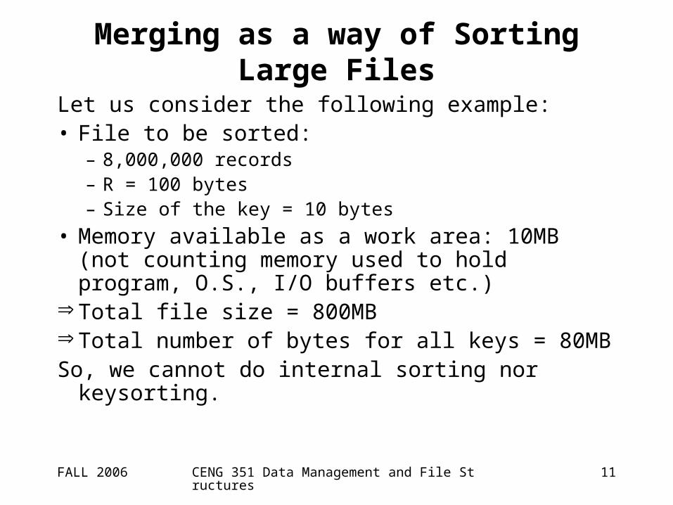
Merging as a way of Sorting Large Files

Let us consider the following example:• File to be sorted:

– 8,000,000 records– R = 100 bytes– Size of the key = 10 bytes

• Memory available as a work area: 10MB (not counting memory used to hold program, O.S., I/O buffers etc.)

Total file size = 800MB Total number of bytes for all keys = 80MBSo, we cannot do internal sorting nor keysorting.


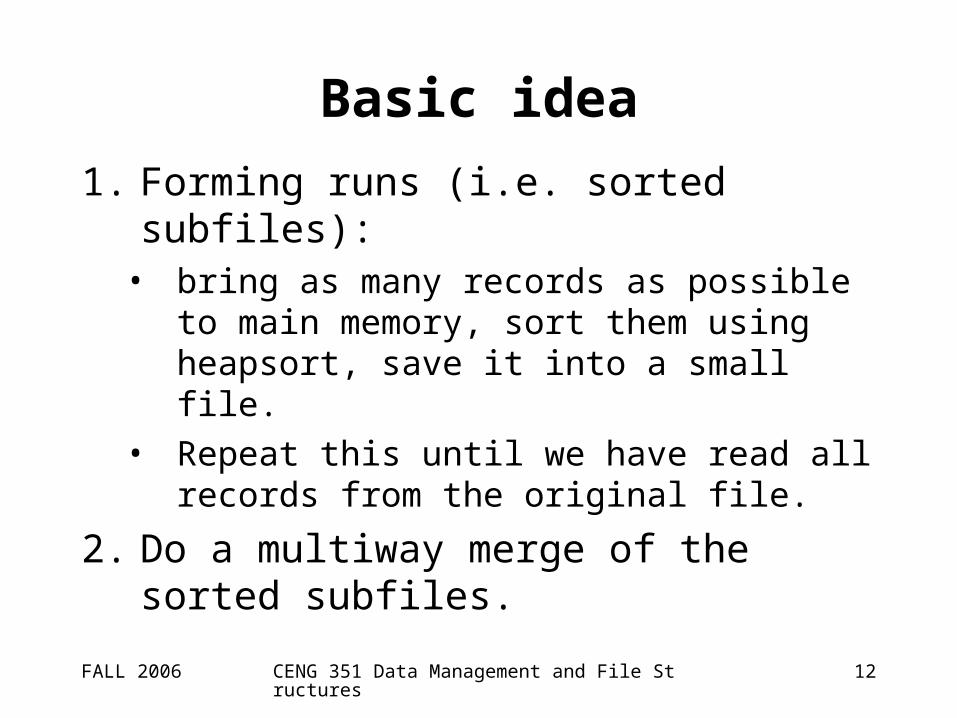
Basic idea

1. Forming runs (i.e. sorted subfiles): • bring as many records as possible to main

memory, sort them using heapsort, save it into a small file.

• Repeat this until we have read all records from the original file.

2. Do a multiway merge of the sorted subfiles.


Cost of Merge Sort

I/O operations are performed in the following times:

1. Reading each record into main memory for sorting and forming the runs.

2. Writing sorted runs to disk.

These two steps are done as follows:– Read a chunk of 10MB, write a chunk of 10Mb

(repeat this 80 times)

– In terms of basic disk operations, we spend:• For reading: 80 seeks + transfer time for 800 MB

• Same for writing


3. Reading runs into memory for merging. Read one chunk of each run, so 80 chunks. Since available memory is 10MB each chunk can have (10,000,000/80)bytes = 125,000 bytes = 1250 records.

• How many chunks to be read for each run?

Size of run/size of chunk = 10,000,000/125,000= 80

• Total number of basic seeks = Total number of chunks (counting all runs) is 80 runs * 80 chunks/run = 802 chunks = 6400 seeks.

• Reading each chunk involves average seeking.


4. Writing sorted file to disk: after the first pass, the number of separate writes closely approximate reads. We estimate two seeks - one for reading and one for writing- for each piece: 80* 80 pieces therefore

6400 seeks


Sorting a File that is 10 times larger

• How is the time for merge phase affected if the file is 80 million records?– More runs: 800 runs– 800-way merge in 10MB memory– i.e. divide the memory into 800 buffers.– Each buffer holds 1/800th of a run– So, 800 runs * 800 seeks/run = 640,000 seeks


The cost of increasing the file size

• In general, for a K-way merge of K runs, the buffer size for each run is– (1/K) * size of memory space = (1/K) * size of each run

• So K seeks are required to read all of the records in each run.

• Since there are K runs, merge requires K2 seeks.• Because K is directly proportional to N it also

follows that the sort merge is an O(N2) operation.


Improvements

There are several ways to reduce the time:

1. Allocate more hardware (e.g. Disk drives, memory)

2. Perform merge in more than one step.

3. Algorithmically increase the lengths of the initial sorted runs

4. Find ways to overlap I/O operations.


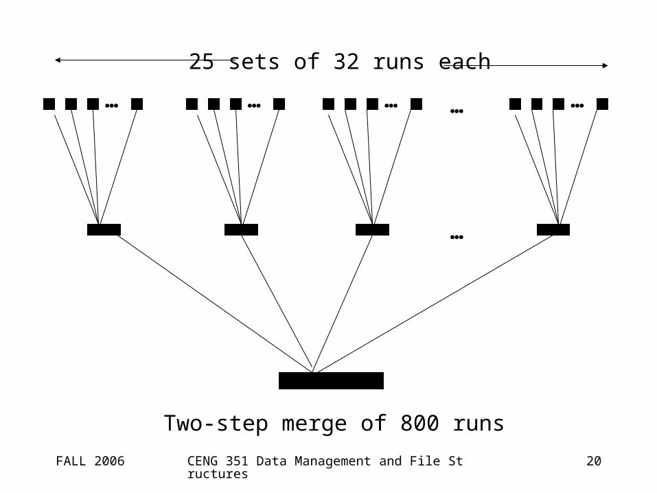
Multiple-step merges

• Instead of merging all runs at once, we break the original set of runs into small groups and merge the runs in these groups separately.– more buffer space is available for each run;

hence fewer seeks are required per run.

• When all of the smaller merges are completed, a second pass merges the new set of merged runs.


…… …… …

…

25 sets of 32 runs each

Two-step merge of 800 runs


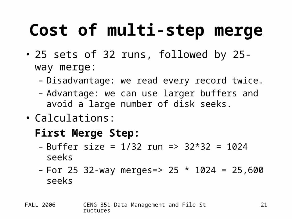
Cost of multi-step merge

• 25 sets of 32 runs, followed by 25-way merge:– Disadvantage: we read every record twice.

– Advantage: we can use larger buffers and avoid a large number of disk seeks.

• Calculations:

First Merge Step:– Buffer size = 1/32 run => 32*32 = 1024 seeks

– For 25 32-way merges=> 25 * 1024 = 25,600 seeks


Second Merge Step:– For each 25 final runs, 1/25 buffer space is allocated.– So each input buffer can hold 4000 records (or 1/800

run)– Hence, 800 seeks per run, so we end up making 25 *

800 = 20,000 seeks.

Total number of seeks for reading in two steps:25600 + 20000 = 45,600

• What about the total time for merge?– We now have to transmit all of the records 4 times

instead of two.– We also write the records twice, requiring an extra

45,600 seeks.

• Still the trade is profitable (see sections 8.5.1-8.5.5 for actual times)


Increasing Run Lengths

• Assume initial runs contain 200000 records.Then instead of 800-way merge we need 400-way merge.

• A longer initial run means – fewer total runs, – a lower-order merge, – bigger buffers, – fewer seeks.

• How can we create initial runs that are twice as large as the number of records that we can hold in memory?

• => Replacement selection


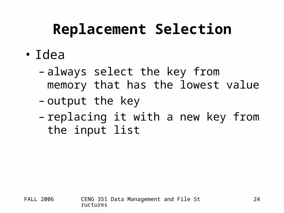
Replacement Selection

• Idea– always select the key from memory that has the

lowest value– output the key– replacing it with a new key from the input list


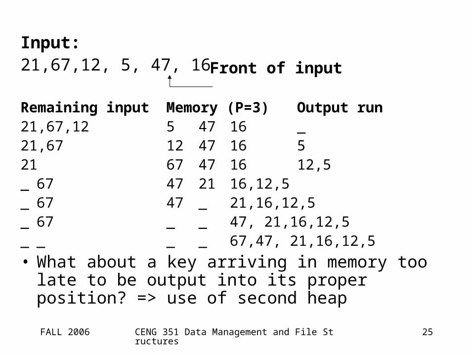
Input:21,67,12, 5, 47, 16

Remaining input Memory (P=3) Output run21,67,12 5 47 16 _21,67 12 47 16 521 67 47 16 12,5_ 67 47 21 16,12,5_ 67 47 _ 21,16,12,5_ 67 _ _ 47, 21,16,12,5_ _ _ _ 67,47, 21,16,12,5

• What about a key arriving in memory too late to be output into its proper position? => use of second heap

Front of input


Trace of replacement selection

Input: ( P = 3)

33, 18, 24,58,14,17,7,21,67,12,5,47,16


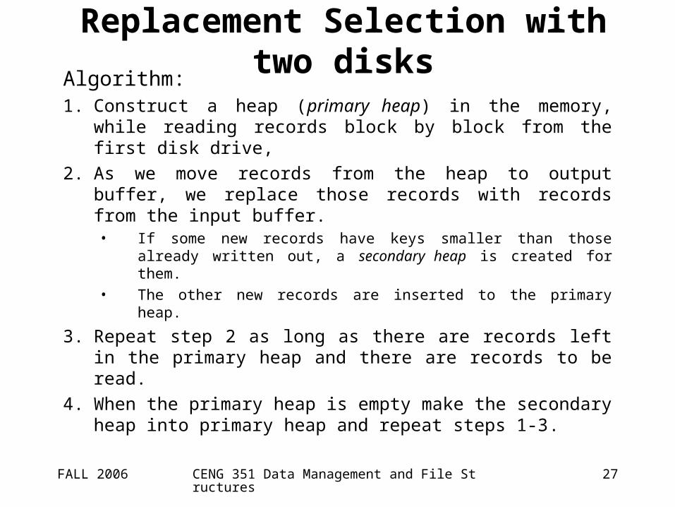
Replacement Selection with two disksAlgorithm:1. Construct a heap (primary heap) in the memory, while

reading records block by block from the first disk drive,

2. As we move records from the heap to output buffer, we replace those records with records from the input buffer.

• If some new records have keys smaller than those already written out, a secondary heap is created for them.

• The other new records are inserted to the primary heap.

3. Repeat step 2 as long as there are records left in the primary heap and there are records to be read.

4. When the primary heap is empty make the secondary heap into primary heap and repeat steps 1-3.

FALL 2006CENG 351 Data Management and File Structures1 External Sorting.

Documents

data management

file structures5

entire file

file doesnt

heap processing

heap property

file structures8 heapsort

file structures4 heapsort