Faint Galaxies in Deep Advanced Camera for Surveys Observations

FAINT GALAXIES IN DEEP ADVANCED CAMERA FOR SURVEYS OBSERVATIONS

N. BenI´tez,1H. Ford,

1R. Bouwens,

2F. Menanteau,

1J. Blakeslee,

1C. Gronwall,

3G. Illingworth,

2G. Meurer,

1

T. J. Broadhurst,4M. Clampin,

5M. Franx,

6G. F. Hartig,

5D. Magee,

2M. Sirianni,

1D. R. Ardila

1F. Bartko,

7

R. A. Brown,5C. J. Burrows,

5E. S. Cheng,

8N. J. G. Cross,

1P. D. Feldman,

1D. A. Golimowski,

1

L. Infante9R. A. Kimble,

8J. E. Krist,

5M. P. Lesser,

10Z. Levay,

5A. R. Martel,

1

G. K. Miley,6M. Postman,

5P. Rosati,

11W. B. Sparks,

5H. D. Tran,

1

Z. I. Tsvetanov,1R. L. White,

1,5and W. Zheng

1

Received 2003 July 17; accepted 2003 August 30

ABSTRACT

We present the analysis of the faint galaxy population in the Advanced Camera for Surveys (ACS) Early ReleaseObservation fields VV 29 (UGC 10214) and NGC 4676. These observations cover a total area of 26.3 arcmin2 andhave depths close to that of the Hubble Deep Fields in the deepest part of the VV 29 image, with 10 � detectionlimits for point sources of 27.8, 27.6, and 27.2 AB magnitudes in the gF475W, VF606W, and IF814W bands,respectively.

Measuring the faint galaxy number count distribution is a difficult task, with different groups arriving at widelyvarying results even on the same data set. Here we attempt to thoroughly consider all aspects relevant for faintgalaxy counting and photometry, developing methods that are based on public software and that are easilyreproducible by other astronomers. Using simulations we determine the best SExtractor parameters for thedetection of faint galaxies in deep Hubble Space Telescope observations, paying special attention to the issue ofdeblending, which significantly affects the normalization and shape of the number count distribution. We confirm,as claimed by Bernstein, Freedman, & Madore, that Kron-like magnitudes, such as the ones generated bySExtractor, can miss more than half of the light of faint galaxies, what dramatically affects the slope of the numbercounts. We show how to correct for this effect, which depends sensitively not only on the characteristics of theobservations, but also on the choice of SExtractor parameters.

We present catalogs for the VV 29 and NGC 4676 fields with photometry in the F475W, F606W, and F814Wbands. We also show that combining the Bayesian software BPZ with superb ACS data and new spectral templatesenables us to estimate reliable photometric redshifts for a significant fraction of galaxies with as few as three filters.

After correcting for selection effects, we measure slopes of 0:32 � 0:01 for 22 < gF475W < 28, 0:34 � 0:01 for22 < VF606W < 27:5, and 0:33 � 0:01 for 22 < mF814W < 27. The counts do not flatten (except perhaps in theF475W filter), up to the depth of our observations. Our results agree well with those of Bernstein, Freedman, &Madore, who used different data sets and techniques, and show that it is possible to perform consistentmeasurements of galaxy number counts if the selection effects are properly considered. We find that the faintcounts mAB > 25:5 can be well approximated in all our filters by a passive luminosity evolution model based onthe COMBO-17 luminosity function (� ¼ �1:5), with a strong merging rate following the prescription ofGlazebrook et al., �� / ð1þ QzÞ, with Q ¼ 4.

Subject headings: galaxies: evolution — galaxies: fundamental parameters — galaxies: high-redshift —galaxies: photometry — techniques: photometric

On-line material: color figures, machine-readable tables

1. INTRODUCTION

On 2002 March 7, the Advanced Camera for Surveys (ACS;Ford et al. 1998, 2002) was installed in the Hubble SpaceTelescope (HST ) during the space shuttle mission ST-109. ACSis an instrument designed and built with the study of the faintgalaxy population as one of its main goals. Here we describethe processing and analysis of some of the first scienceobservations taken with the ACS Wide Field Camera, calledEarly Release Observations (EROs).

An important result obtained with the WFPC2 observationsof the Hubble Deep Fields (Williams et al. 1996; Casertanoet al. 2000) was the measurement of the galaxy number countdistribution to very faint ðmABk 27Þ limits. However, it isremarkable that different groups have reached differentconclusions about the slope and normalization of the numbercounts even when using the same software on the same data set(see, e.g., Ferguson, Dickinson, & Williams 2000; Vanzellaet al. 2001). One of the few results on which all groups seemedto agree was the flattening of the number counts at IAB � 26.

A

1 Department of Physics and Astronomy, Johns Hopkins University, 3400North Charles Street, Baltimore, MD 21218.

2 UCO/Lick Observatory, University of California, Santa Cruz, CA 95064.3 Department of Astronomy and Astrophysics, Pennsylvania State Uni-

versity, 525 Davey Lab, University Park, PA 16802.4 Racah Institute of Physics, Hebrew University, Jerusalem, Israel 91904.5 Space Telescope Science Institute, 3700 San Martin Drive, Baltimore,

MD 21218.6 Leiden Observatory, Postbus 9513, 2300 RA Leiden, Netherlands.

7 Bartko Science and Technology, P.O. Box 670, Mead, CO 80542-0670.8 NASA Goddard Space Flight Center, Laboratory for Astronomy and Solar

Physics, Greenbelt, MD 20771.9 Departmento de Astronomıa y Astrofısica, Pontificia Universidad Catolica

de Chile, Casilla 306, Santiago 22, Chile.10 Steward Observatory, University of Arizona, Tucson, AZ 85721.11 European Southern Observatory, Karl-Schwarzschild-Strasse 2, D-85748

Garching, Germany.

1

The Astrophysical Journal Supplement Series, 150:1–18, 2004 January

# 2004. The American Astronomical Society. All rights reserved. Printed in U.S.A.

However, Bernstein, Freedman, & Madore (2002a, 2002b,hereafter BFM) claim that this is a spurious effect, caused bythe underestimation of the true luminosity of faint galaxies bystandard aperture measurements, and that the number countscontinue with a slope of 0.33 up to the limits of the HDFN VandI bands.

Two of the main goals of this paper are improving ourunderstanding of the biases and selection effects involved incounting and measuring the properties of very faint galaxies,and developing techniques that can be applied to a wide rangeof observations and that are easily reproduced by otherastronomers. This is essential if galaxy counting is to becomea precise science. We have done this by using almostexclusively public software, and specifying the parametersused, thus ensuring that our results are repeatable.

Our final results are the number counts in the F475W,F606W, and F814W bands, carefully corrected for selectioneffects. Using an independent procedure, we confirm the ap-parent absence of flattening in the number counts found byBFM. We also show that using proper priors, reasonably robustphotometric redshifts can be obtained using only three ACSfilters. Finally, we present photometric catalogs of fieldgalaxies in the VV 29 and NGC 4676 fields.

The structure of the paper is as follows: x 2 describes ourobservations, x 3 deals with the image processing and thegeneration of the catalogs, including the description of thesimulations used to correct our number counts. Section 3 alsolists and explains the quantities included in our catalogs, x 4presents our number counts, and x 5 summarizes our mainresults and conclusions.

2. OBSERVATIONS

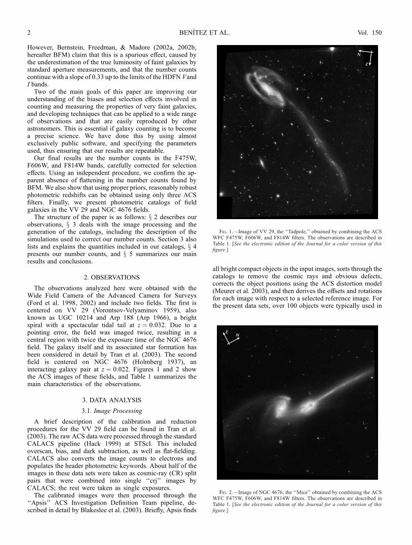
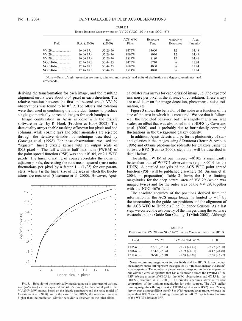
The observations analyzed here were obtained with theWide Field Camera of the Advanced Camera for Surveys(Ford et al. 1998, 2002) and include two fields. The first iscentered on VV 29 (Vorontsov-Velyaminov 1959), alsoknown as UGC 10214 and Arp 188 (Arp 1966), a brightspiral with a spectacular tidal tail at z ¼ 0:032. Due to apointing error, the field was imaged twice, resulting in acentral region with twice the exposure time of the NGC 4676field. The galaxy itself and its associated star formation hasbeen considered in detail by Tran et al. (2003). The secondfield is centered on NGC 4676 (Holmberg 1937), aninteracting galaxy pair at z ¼ 0:022. Figures 1 and 2 showthe ACS images of these fields, and Table 1 summarizes themain characteristics of the observations.

3. DATA ANALYSIS

3.1. Image Processing

A brief description of the calibration and reductionprocedures for the VV 29 field can be found in Tran et al.(2003). The raw ACS data were processed through the standardCALACS pipeline (Hack 1999) at STScI. This includedoverscan, bias, and dark subtraction, as well as flat-fielding.CALACS also converts the image counts to electrons andpopulates the header photometric keywords. About half of theimages in these data sets were taken as cosmic-ray (CR) splitpairs that were combined into single ‘‘crj’’ images byCALACS; the rest were taken as single exposures.

The calibrated images were then processed through the‘‘Apsis’’ ACS Investigation Definition Team pipeline, de-scribed in detail by Blakeslee et al. (2003). Briefly, Apsis finds

all bright compact objects in the input images, sorts through thecatalogs to remove the cosmic rays and obvious defects,corrects the object positions using the ACS distortion model(Meurer et al. 2003), and then derives the offsets and rotationsfor each image with respect to a selected reference image. Forthe present data sets, over 100 objects were typically used in

Fig. 1.—Image of VV 29, the ‘‘Tadpole,’’ obtained by combining the ACSWFC F475W, F606W, and F814W filters. The observations are described inTable 1. [See the electronic edition of the Journal for a color version of thisfigure.]

Fig. 2.—Image of NGC 4676, the ‘‘Mice’’ obtained by combining the ACSWFC F475W, F606W, and F814W filters. The observations are described inTable 1. [See the electronic edition of the Journal for a color version of thisfigure.]

BENITEZ ET AL.2 Vol. 150

deriving the transformation for each image, and the resultingalignment errors were about 0.04 pixel in each direction. Therelative rotation between the first and second epoch VV 29observations was found to be 0B12. The offsets and rotationswere then used in combining the individual frames to producesingle geometrically corrected images for each bandpass.

Image combination in Apsis is done with the drizzlesoftware written by R. Hook (Fruchter & Hook 2002). Thedata quality arrays enable masking of known hot pixels and badcolumns, while cosmic rays and other anomalies are rejectedthrough the iterative drizzle/blot technique described byGonzaga et al. (1998). For these observations, we used the‘‘square’’ (linear) drizzle kernel with an output scale of0B05 pixel�1. The full width at half-maximum (FWHM) ofthe point spread function (PSF) was about 0B105, or 2.1 WFCpixels. The linear drizzling of course correlates the noise inadjacent pixels, decreasing the root mean squared (rms) noisefluctuations per pixel by a factor 1� ð1=3lÞ for our param-eters, where l is the linear size of the area in which the fluctu-ations are measured (Casertano et al. 2000). However, Apsis

calculates rms arrays for each drizzled image, i.e., the expectedrms noise per pixel in the absence of correlation. These arraysare used later on for image detection, photometric noise esti-mation, etc.

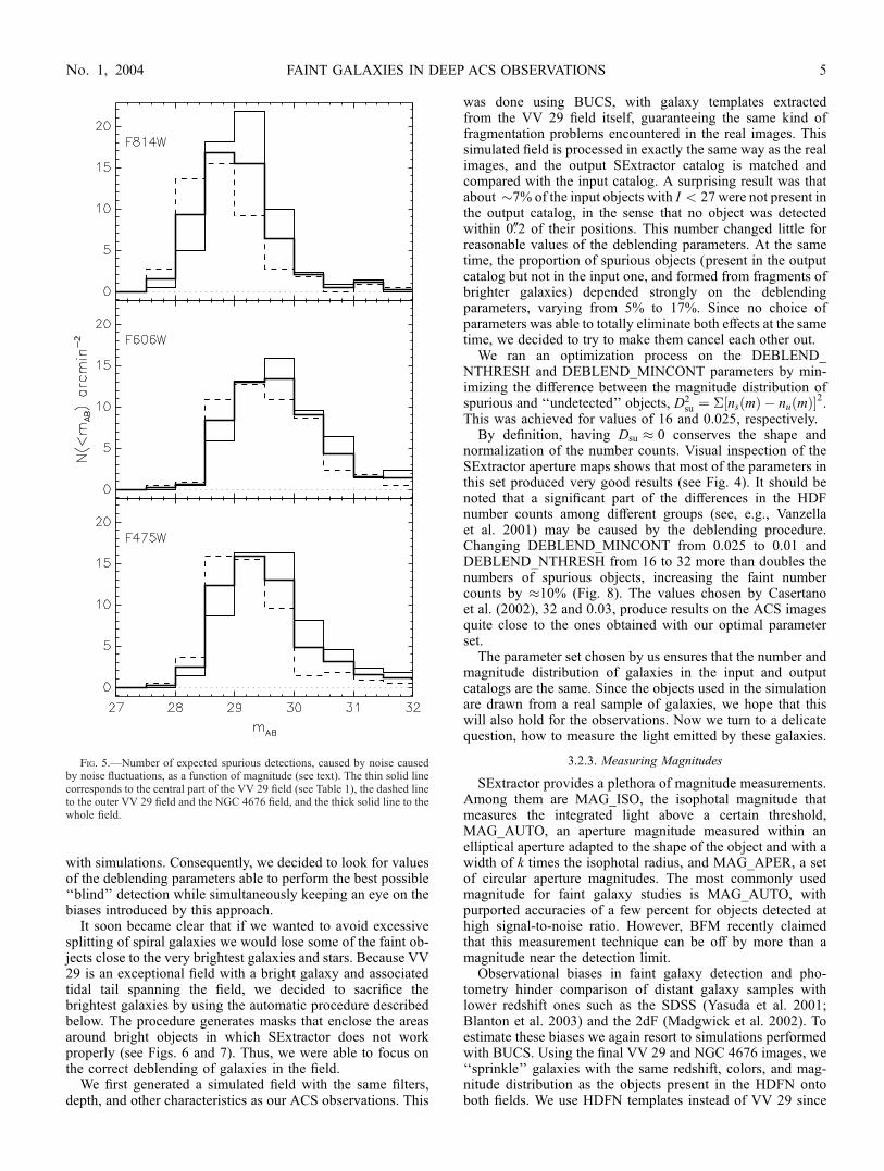
Figure 3 shows the behavior of the noise as a function of thesize of the area in which it is measured. We see that it followswell the predicted behavior, but it is slightly higher on largescales, an effect that was also noted in the HDFS by Casertanoet al. (2000), and is probably due to intrinsically correlatedfluctuations in the background galaxy density.

In addition, Apsis detects and performs photometry of starsand galaxies in the images using SExtractor (Bertin & Arnouts1996) and obtains photometric redshifts for galaxies using thesoftware BPZ (Benıtez 2000), steps that will be described indetail below.

The stellar FWHM of our images, �0B105 is significantlybetter than that of WFPC2 observations (e.g., �0B14 for theHDFS). A detailed analysis of the ACS WFC point spreadfunction (PSF) will be published elsewhere (M. Sirianni et al.2004, in preparation). Table 2 shows the 10 � limitingmagnitudes for the deep central area of VV 29 (which wasimaged twice) and for the outer area of the VV 29, togetherwith the NGC 4676 field.

The absolute accuracy of the positions derived from theinformation in the ACS image header is limited to �100 bythe uncertainty in the guide star positions and the alignment ofthe ACS WFC to Hubble’s Fine Guidance Sensors. As a laststep, we correct the astrometry of the images using the softwarewcstools and the Guide Star Catalog II (Mink 2002). Although

Fig. 3.—Behavior of the empirically measured noise in apertures of varyingsize (solid line) vs. the expected one (dashed line), for the central part of theVV 29 F475W images, based on the drizzle parameters and the noise model ofCasertano et al. (2000). As in the case of the HDFN, the measured noise ishigher than the prediction. Similar behavior is observed in the other filters.

TABLE 1

Early Release Observations of VV 29 (UGC 10214) and NGC 4676

Field R.A. (J2000)Decl.(J2000)

ACS WFC

Filter

Exposure

TimeNumber ofExposures

Area

(arcmin2)

VV 29 ........................ 16 06 17.4 55 26 46 F475W 13600 12 14.48

VV 29 ........................ 16 06 17.4 55 26 46 F606W 8040 12 14.49

VV 29 ........................ 16 06 17.4 55 26 46 F814W 8180 12 14.46

NGC 4676.................. 12 46 09.0 30 44 25 F475W 6740 6 11.84

NGC 4676.................. 12 46 09.0 30 44 25 F606W 4000 6 11.84

NGC 4676.................. 12 46 09.0 30 44 25 F814W 4070 6 11.84

Note.—Units of right ascension are hours, minutes, and seconds, and units of declination are degrees, arcminutes, andarcseconds.

TABLE 2

Depth of the VV 29 and NGC 4676 Fields Compared with the HDFS

Band VV 29 VV 29/NGC 4676 HDFS

F475W...... 27.61 (27.83) 27.23 (27.45) 27.97 (27.90)

F606W...... 27.42 (27.64) 27.09 (27.31) 28.47 (28.40)

F814W...... 26.98 (27.20) 26.58 (26.80) 27.84 (27.77)

Notes.—Limiting magnitudes for our fields and the HDFS. In each entry,the numbers on the left represent the expected 10 � fluctuation in an 0.2 arcsec2

square aperture. The number in parentheses corresponds to the same quantity,but within a circular aperture that has a diameter 4 times the FWHM of thePSF. We use a value of 0B105 for the WFC observations and 0B135 for theHDFS (Casertano et al. 2000). The circular apertures allow a realisticcomparison of the limiting magnitudes for point sources. The ACS stellarlimiting magnitude through the 4� FWHM aperture (d � 0B42) is�0.22 magfainter than a source filling the 0B45� 0B45 rectangular aperture, whereas theequivalent WFC2 stellar limiting magnitude is �0.07 mag brighter becauseof the WFC2’s broader PSF.

FAINT GALAXIES IN DEEP ACS OBSERVATIONS 3No. 1, 2004

there are not many cataloged stars in our images, visualinspection shows that our corrected positions should be accu-rate to P0B1.

The reduced images in the three filters, together withauxiliary images (detection image, rms images) are availableon-line12.

3.2. Galaxy Identification and Photometry

3.2.1. Object Detection

SExtractor (Bertin & Arnouts 1996) has become the de factostandard for automated faint galaxy detection and photometry.It finds objects using a connected pixel approach, includingweight and flag maps if desired, and provides the user withefficient and accurate measurements of the most widely usedobject properties. As stated previously, one of our main goals isto understand in detail how the process of galaxy detection andanalysis affect the shape of the number counts distribution, andthen use this understanding to arrive at results that are asobjective as possible. To achieve our goal, we carefully chooseour SExtractor parameters, and most importantly, characterizethe biases and errors by using extensive simulations with thepublic software BUCS (Bouwens Universe Construction Set;see Appendix A and Bouwens, Broadhurst, & Illingworth 2003for a detailed description). This approach will allow otherastronomers to contrast and compare our results with their ownin a consistent way. Because the output of SExtractor sen-sitively depends on its input parameters, we present ourparameters in Appendix B to ensure that others can repeat ouranalysis.

One of SExtractor’s more convenient features is the doubleimage mode. This mode enables object detection and aperturedefinition in one image, and aperture photometry in a differentimage. To create our detection image, we use an inversevariance weighted average of the F475W, F606W, and F814Wimages. This differs from the procedure followed for the HDFsby other authors, who usually only use the reddest bands,F606W and F814W. However, we think that inclusion of theF475W image is justified since it is the deepest of the three; in

fact, Table 2 shows that the F475W image is almost as deep asthe HDFS for point sources. The PSF in the final detectionimage is basically identical to that of the F606W image anddiffers by less than 2% from the stellar width of the B and Ifilters.Although there are roughly 13 parameters that influence the

detection process in SExtractor, the most critical ones areDETECTMINAREA, the minimum number of connectedpixels and DETECTTHRESH, the detection threshold abovethe background. We performed tests to select these parameters,ensuring that we recovered all obvious galaxies in the fieldwhile not producing large numbers of spurious detections. Wechose the rather conservative limits of DETECTMINAREA ¼5 and DETECTTHRESH ¼ 1:5 (which provides a nominalS=N ¼ 3:35), because we think that given the limited scientificinformation to be extracted from the sources close to thedetection limit, it is better to avoid adulterating our catalogswith large numbers of false sources. Figure 4 shows the resultsof a SExtractor run in a portion of the VV 29 field. To estimatethe number of isolated spurious detections, we subtracted themean sky and changed the sign of all pixels in our images andran SExtractor on them with the same parameters andconfiguration as described in Appendix B. The number ofspurious detections for mAB < 28 is very small in all filters, aswe can see in Figure 5, but they have nevertheless beencorrected for in the final number counts results.

3.2.2. Object Deblending

Two other very important parameters that govern thedeblending process are DEBLEND_NTHRESH andDEBLEND_MINCONT. Typical values used by other authorsare, respectively, 32 and 0.01–0.03. At least two teams usingHDFN data performed part of the detection/deblending processwith manual intervention (Casertano et al. 2000; Vanzella et al.2001). This approach may be valid for an isolated field, but wethink that it should not be applied to a large set of observationssuch as the ones that will be produced by the ACS GTOprogram. Not only does manual intervention require consid-erable effort, it also introduces subjective biases and possibleinconsistencies that make repeatability by other groupsdifficult, as well as complicating quantification of the errors

Fig. 4.—Example of SExtractor object finding and deblending on a section of the VV 29 field. The displayed apertures are the ones corresponding to SExtractorMAG_AUTO magnitudes.

12 See http://acs.pha.jhu.edu.


with simulations. Consequently, we decided to look for valuesof the deblending parameters able to perform the best possible‘‘blind’’ detection while simultaneously keeping an eye on thebiases introduced by this approach.

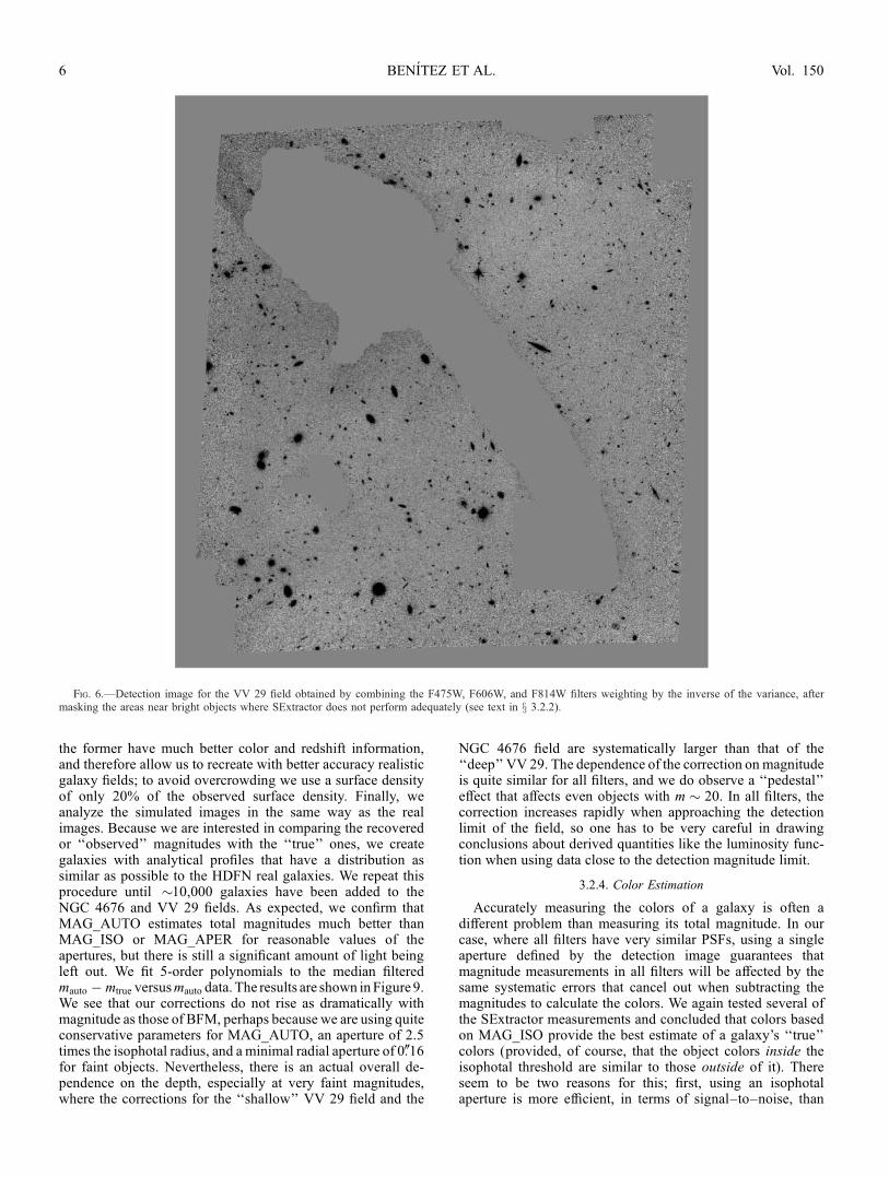
It soon became clear that if we wanted to avoid excessivesplitting of spiral galaxies we would lose some of the faint ob-jects close to the very brightest galaxies and stars. Because VV29 is an exceptional field with a bright galaxy and associatedtidal tail spanning the field, we decided to sacrifice thebrightest galaxies by using the automatic procedure describedbelow. The procedure generates masks that enclose the areasaround bright objects in which SExtractor does not workproperly (see Figs. 6 and 7). Thus, we were able to focus onthe correct deblending of galaxies in the field.

We first generated a simulated field with the same filters,depth, and other characteristics as our ACS observations. This

was done using BUCS, with galaxy templates extractedfrom the VV 29 field itself, guaranteeing the same kind offragmentation problems encountered in the real images. Thissimulated field is processed in exactly the same way as the realimages, and the output SExtractor catalog is matched andcompared with the input catalog. A surprising result was thatabout �7% of the input objects with I < 27 were not present inthe output catalog, in the sense that no object was detectedwithin 0B2 of their positions. This number changed little forreasonable values of the deblending parameters. At the sametime, the proportion of spurious objects (present in the outputcatalog but not in the input one, and formed from fragments ofbrighter galaxies) depended strongly on the deblendingparameters, varying from 5% to 17%. Since no choice ofparameters was able to totally eliminate both effects at the sametime, we decided to try to make them cancel each other out.

We ran an optimization process on the DEBLEND_NTHRESH and DEBLEND_MINCONT parameters by min-imizing the difference between the magnitude distribution ofspurious and ‘‘undetected’’ objects, D2

su ¼ �½nsðmÞ � nuðmÞ�2.This was achieved for values of 16 and 0.025, respectively.

By definition, having Dsu � 0 conserves the shape andnormalization of the number counts. Visual inspection of theSExtractor aperture maps shows that most of the parameters inthis set produced very good results (see Fig. 4). It should benoted that a significant part of the differences in the HDFnumber counts among different groups (see, e.g., Vanzellaet al. 2001) may be caused by the deblending procedure.Changing DEBLEND_MINCONT from 0.025 to 0.01 andDEBLEND_NTHRESH from 16 to 32 more than doubles thenumbers of spurious objects, increasing the faint numbercounts by �10% (Fig. 8). The values chosen by Casertanoet al. (2002), 32 and 0.03, produce results on the ACS imagesquite close to the ones obtained with our optimal parameterset.

The parameter set chosen by us ensures that the number andmagnitude distribution of galaxies in the input and outputcatalogs are the same. Since the objects used in the simulationare drawn from a real sample of galaxies, we hope that thiswill also hold for the observations. Now we turn to a delicatequestion, how to measure the light emitted by these galaxies.

3.2.3. Measuring Magnitudes

SExtractor provides a plethora of magnitude measurements.Among them are MAG_ISO, the isophotal magnitude thatmeasures the integrated light above a certain threshold,MAG_AUTO, an aperture magnitude measured within anelliptical aperture adapted to the shape of the object and with awidth of k times the isophotal radius, and MAG_APER, a setof circular aperture magnitudes. The most commonly usedmagnitude for faint galaxy studies is MAG_AUTO, withpurported accuracies of a few percent for objects detected athigh signal-to-noise ratio. However, BFM recently claimedthat this measurement technique can be off by more than amagnitude near the detection limit.

Observational biases in faint galaxy detection and pho-tometry hinder comparison of distant galaxy samples withlower redshift ones such as the SDSS (Yasuda et al. 2001;Blanton et al. 2003) and the 2dF (Madgwick et al. 2002). Toestimate these biases we again resort to simulations performedwith BUCS. Using the final VV 29 and NGC 4676 images, we‘‘sprinkle’’ galaxies with the same redshift, colors, and mag-nitude distribution as the objects present in the HDFN ontoboth fields. We use HDFN templates instead of VV 29 since

Fig. 5.—Number of expected spurious detections, caused by noise causedby noise fluctuations, as a function of magnitude (see text). The thin solid linecorresponds to the central part of the VV 29 field (see Table 1), the dashed lineto the outer VV 29 field and the NGC 4676 field, and the thick solid line to thewhole field.


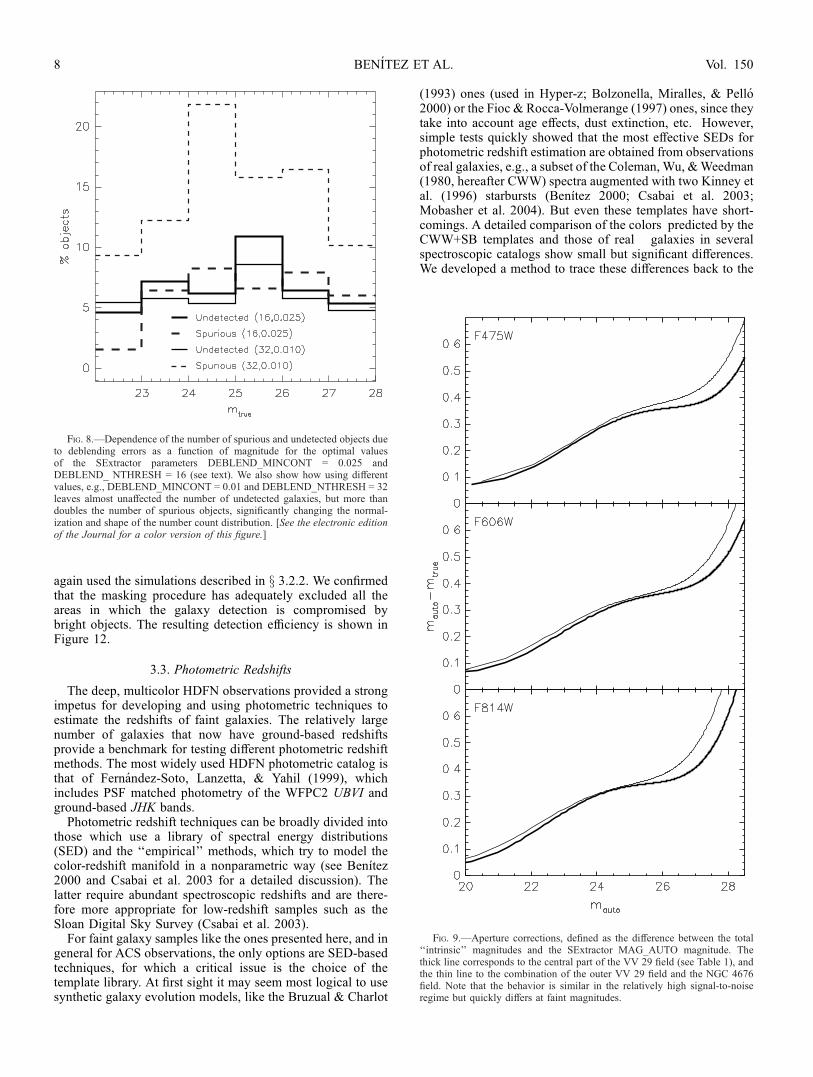
the former have much better color and redshift information,and therefore allow us to recreate with better accuracy realisticgalaxy fields; to avoid overcrowding we use a surface densityof only 20% of the observed surface density. Finally, weanalyze the simulated images in the same way as the realimages. Because we are interested in comparing the recoveredor ‘‘observed’’ magnitudes with the ‘‘true’’ ones, we creategalaxies with analytical profiles that have a distribution assimilar as possible to the HDFN real galaxies. We repeat thisprocedure until �10,000 galaxies have been added to theNGC 4676 and VV 29 fields. As expected, we confirm thatMAG_AUTO estimates total magnitudes much better thanMAG_ISO or MAG_APER for reasonable values of theapertures, but there is still a significant amount of light beingleft out. We fit 5-order polynomials to the median filteredmauto � mtrue versusmauto data. The results are shown inFigure 9.We see that our corrections do not rise as dramatically withmagnitude as those of BFM, perhaps because we are using quiteconservative parameters for MAG_AUTO, an aperture of 2.5times the isophotal radius, and a minimal radial aperture of 0B16for faint objects. Nevertheless, there is an actual overall de-pendence on the depth, especially at very faint magnitudes,where the corrections for the ‘‘shallow’’ VV 29 field and the

NGC 4676 field are systematically larger than that of the‘‘deep’’ VV 29. The dependence of the correction on magnitudeis quite similar for all filters, and we do observe a ‘‘pedestal’’effect that affects even objects with m � 20. In all filters, thecorrection increases rapidly when approaching the detectionlimit of the field, so one has to be very careful in drawingconclusions about derived quantities like the luminosity func-tion when using data close to the detection magnitude limit.

3.2.4. Color Estimation

Accurately measuring the colors of a galaxy is often adifferent problem than measuring its total magnitude. In ourcase, where all filters have very similar PSFs, using a singleaperture defined by the detection image guarantees thatmagnitude measurements in all filters will be affected by thesame systematic errors that cancel out when subtracting themagnitudes to calculate the colors. We again tested several ofthe SExtractor measurements and concluded that colors basedon MAG_ISO provide the best estimate of a galaxy’s ‘‘true’’colors (provided, of course, that the object colors inside theisophotal threshold are similar to those outside of it). Thereseem to be two reasons for this; first, using an isophotalaperture is more efficient, in terms of signal–to–noise, than

Fig. 6.—Detection image for the VV 29 field obtained by combining the F475W, F606W, and F814W filters weighting by the inverse of the variance, aftermasking the areas near bright objects where SExtractor does not perform adequately (see text in x 3.2.2).


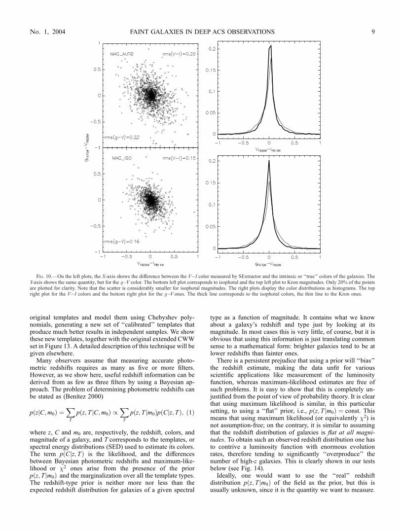
MAG_AUTO, which integrates the light distribution overregions in which the noise is dominant. Second, althoughSExtractor tries to correct its aperture magnitude measurementsfor the presence of nearby objects, it does not always do sosuccessfully, and there are a significant number of cases inwhich the magnitudes are strongly contaminated by the lightfrom close companions. Isophotal magnitudes are largely freeof this problem. The comparisons between MAG_ISO andMAG_AUTO are shown in Figure 10. For bright, compactobjects a small aperture with a diameter of 0B15 works slightlybetter than MAG_ISO, but its performance is equal or slightlyworse for fainter objects, so we decided to use MAG_ISO forall objects.

As expected, the advantages of isophotal magnitudesfor estimating colors also are evident in the photometricredshifts. On average, we can estimate reliable photometricredshifts for 11% more objects if we use MAG_ISO insteadof MAG_AUTO (see x 3.3).

We show color-color plots, together with the trackscorresponding to some of the templates introduced below, inFigure 11.

3.2.5. Completeness Corrections

We previously noted that SExtractor is not designed to worknear very bright objects and in general will produce numerous

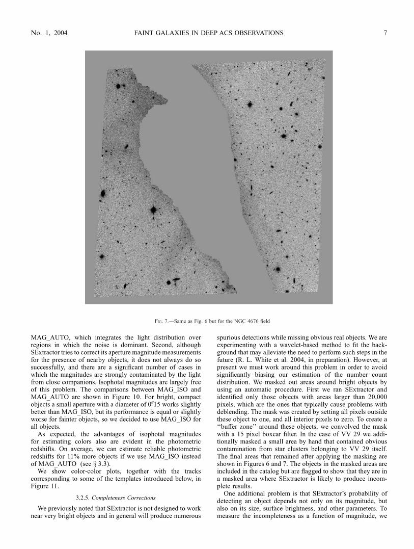
spurious detections while missing obvious real objects. We areexperimenting with a wavelet-based method to fit the back-ground that may alleviate the need to perform such steps in thefuture (R. L. White et al. 2004, in preparation). However, atpresent we must work around this problem in order to avoidsignificantly biasing our estimation of the number countdistribution. We masked out areas around bright objects byusing an automatic procedure. First we ran SExtractor andidentified only those objects with areas larger than 20,000pixels, which are the ones that typically cause problems withdeblending. The mask was created by setting all pixels outsidethese object to one, and all interior pixels to zero. To create a‘‘buffer zone’’ around these objects, we convolved the maskwith a 15 pixel boxcar filter. In the case of VV 29 we addi-tionally masked a small area by hand that contained obviouscontamination from star clusters belonging to VV 29 itself.The final areas that remained after applying the masking areshown in Figures 6 and 7. The objects in the masked areas areincluded in the catalog but are flagged to show that they are ina masked area where SExtractor is likely to produce incom-plete results.

One additional problem is that SExtractor’s probability ofdetecting an object depends not only on its magnitude, butalso on its size, surface brightness, and other parameters. Tomeasure the incompleteness as a function of magnitude, we

Fig. 7.—Same as Fig. 6 but for the NGC 4676 field


again used the simulations described in x 3.2.2. We confirmedthat the masking procedure has adequately excluded all theareas in which the galaxy detection is compromised bybright objects. The resulting detection efficiency is shown inFigure 12.

3.3. Photometric Redshifts

The deep, multicolor HDFN observations provided a strongimpetus for developing and using photometric techniques toestimate the redshifts of faint galaxies. The relatively largenumber of galaxies that now have ground-based redshiftsprovide a benchmark for testing different photometric redshiftmethods. The most widely used HDFN photometric catalog isthat of Fernandez-Soto, Lanzetta, & Yahil (1999), whichincludes PSF matched photometry of the WFPC2 UBVI andground-based JHK bands.

Photometric redshift techniques can be broadly divided intothose which use a library of spectral energy distributions(SED) and the ‘‘empirical’’ methods, which try to model thecolor-redshift manifold in a nonparametric way (see Benıtez2000 and Csabai et al. 2003 for a detailed discussion). Thelatter require abundant spectroscopic redshifts and are there-fore more appropriate for low-redshift samples such as theSloan Digital Sky Survey (Csabai et al. 2003).

For faint galaxy samples like the ones presented here, and ingeneral for ACS observations, the only options are SED-basedtechniques, for which a critical issue is the choice of thetemplate library. At first sight it may seem most logical to usesynthetic galaxy evolution models, like the Bruzual & Charlot

(1993) ones (used in Hyper-z; Bolzonella, Miralles, & Pello2000) or the Fioc & Rocca-Volmerange (1997) ones, since theytake into account age effects, dust extinction, etc. However,simple tests quickly showed that the most effective SEDs forphotometric redshift estimation are obtained from observationsof real galaxies, e.g., a subset of the Coleman, Wu, &Weedman(1980, hereafter CWW) spectra augmented with two Kinney etal. (1996) starbursts (Benıtez 2000; Csabai et al. 2003;Mobasher et al. 2004). But even these templates have short-comings. A detailed comparison of the colors predicted by theCWW+SB templates and those of real galaxies in severalspectroscopic catalogs show small but significant differences.We developed a method to trace these differences back to the

Fig. 8.—Dependence of the number of spurious and undetected objects dueto deblending errors as a function of magnitude for the optimal valuesof the SExtractor parameters DEBLEND_MINCONT = 0.025 andDEBLEND_ NTHRESH = 16 (see text). We also show how using differentvalues, e.g., DEBLEND_MINCONT = 0.01 and DEBLEND_NTHRESH = 32leaves almost unaffected the number of undetected galaxies, but more thandoubles the number of spurious objects, significantly changing the normal-ization and shape of the number count distribution. [See the electronic editionof the Journal for a color version of this figure.]

Fig. 9.—Aperture corrections, defined as the difference between the total‘‘intrinsic’’ magnitudes and the SExtractor MAG_AUTO magnitude. Thethick line corresponds to the central part of the VV 29 field (see Table 1), andthe thin line to the combination of the outer VV 29 field and the NGC 4676field. Note that the behavior is similar in the relatively high signal-to-noiseregime but quickly differs at faint magnitudes.


original templates and model them using Chebyshev poly-nomials, generating a new set of ‘‘calibrated’’ templates thatproduce much better results in independent samples. We showthese new templates, together with the original extended CWWset in Figure 13. A detailed description of this technique will begiven elsewhere.

Many observers assume that measuring accurate photo-metric redshifts requires as many as five or more filters.However, as we show here, useful redshift information can bederived from as few as three filters by using a Bayesian ap-proach. The problem of determining photometric redshifts canbe stated as (Benıtez 2000)

pðzjC;m0Þ ¼X

T

pðz; T jC;m0Þ /X

T

pðz; T jm0ÞpðCjz; TÞ; ð1Þ

where z, C and m0 are, respectively, the redshift, colors, andmagnitude of a galaxy, and T corresponds to the templates, orspectral energy distributions (SED) used to estimate its colors.The term pðCjz; TÞ is the likelihood, and the differencesbetween Bayesian photometric redshifts and maximum-like-lihood or �2 ones arise from the presence of the priorpðz; T jm0Þ and the marginalization over all the template types.The redshift-type prior is neither more nor less than theexpected redshift distribution for galaxies of a given spectral

type as a function of magnitude. It contains what we knowabout a galaxy’s redshift and type just by looking at itsmagnitude. In most cases this is very little, of course, but it isobvious that using this information is just translating commonsense to a mathematical form: brighter galaxies tend to be atlower redshifts than fainter ones.

There is a persistent prejudice that using a prior will ‘‘bias’’the redshift estimate, making the data unfit for variousscientific applications like measurement of the luminosityfunction, whereas maximum-likelihood estimates are free ofsuch problems. It is easy to show that this is completely un-justified from the point of view of probability theory. It is clearthat using maximum likelihood is similar, in this particularsetting, to using a ‘‘flat’’ prior, i.e., pðz; T jm0Þ ¼ const. Thismeans that using maximum likelihood (or equivalently �2) isnot assumption-free; on the contrary, it is similar to assumingthat the redshift distribution of galaxies is flat at all magni-tudes. To obtain such an observed redshift distribution one hasto contrive a luminosity function with enormous evolutionrates, therefore tending to significantly ‘‘overproduce’’ thenumber of high-z galaxies. This is clearly shown in our testsbelow (see Fig. 14).

Ideally, one would want to use the ‘‘real’’ redshiftdistribution pðz; T jm0Þ of the field as the prior, but this isusually unknown, since it is the quantity we want to measure.

Fig. 10.—On the left plots, the X-axis shows the difference between the V�I color measured by SExtractor and the intrinsic or ‘‘true’’ colors of the galaxies. TheY-axis shows the same quantity, but for the g�V color. The bottom left plot corresponds to isophotal and the top left plot to Kron magnitudes. Only 20% of the pointsare plotted for clarity. Note that the scatter is considerably smaller for isophotal magnitudes. The right plots display the color distributions as histograms. The topright plot for the V�I colors and the bottom right plot for the g�V ones. The thick line corresponds to the isophotal colors, the thin line to the Kron ones.


But it is clear that an analytical fit to the redshift histogramfrom a similar blank field, like the HDFN, is always a muchbetter approximation—in spite of the cosmic variance—thana flat redshift distribution. Thus, using empirical priors suchas the ones introduced in Benıtez (2000), does in fact con-siderably reduce the biases introduced by maximum-likeli-hood methods. Simple comparisons like the one below usingthe same data set and template sets show that, as expected,Bayesian probability gives consistently more accurate andreliable results than maximum-likelihood or �2 techniques

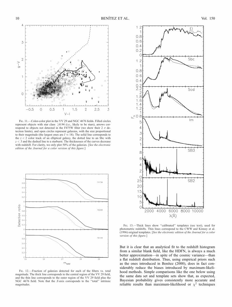
Fig. 11.—Color-color plot in the VV 29 and NGC 4676 fields. Filled circlesrepresent objects with star class �0.94 (i.e., likely to be stars), arrows cor-respond to objects not detected in the F475W filter (we show their 2 � de-tection limits), and open circles represent galaxies, with the size proportionalto their magnitude (the largest ones are I � 18). The solid line corresponds tothe z < 2 color track of an elliptical galaxy, the dotted line to an Sbc withz < 3 and the dashed line to a starburst. The thicknesses of the curves decreasewith redshift. For clarity, we only plot 50% of the galaxies. [See the electronicedition of the Journal for a color version of this figure.]

Fig. 12.—Fraction of galaxies detected for each of the filters vs. totalmagnitude. The thick line corresponds to the central region of the VV 29 field,and the thin line corresponds to the outer region of the VV 29 field plus theNGC 4676 field. Note that the X-axis corresponds to the ‘‘total’’ intrinsicmagnitudes.

Fig. 13.—Thick lines show ‘‘calibrated’’ templates (see text), used forphotometric redshifts. Thin lines correspond to the CWW and Kinney et al.(1996) original templates. [See the electronic edition of the Journal for a colorversion of this figure.]


(see also Benıtez 2000; Csabai et al. 2003; Mobasher et al.2004).

To test how well we can expect to estimate photometricredshifts with our data, we performed the following test. We ranBPZ with the same set of parameters described in Appendix C,but using only the WFPC2 BVI photometry from the Fernan-dez-Soto et al. (1999) catalog. This is almost identical in filtercoverage and depth to the observations discussed here and

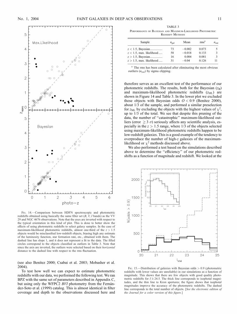
therefore serves as an excellent test of the performance of ourphotometric redshifts. The results, both for the Bayesian (zB)and maximum-likelihood photometric redshifts (zML) areshown in Figure 14 and Table 3. In the lower plot we excludedthose objects with Bayesian odds O < 0:9 (Benıtez 2000),about 1/3 of the sample, and performed a similar preselectionfor zML by excluding the objects with the highest values of �2,up to 1/3 of the total. We see that despite this pruning of thedata, the number of ‘‘catastrophic’’ maximum-likelihood out-liers (error � 3 �) seriously affects any scientific analysis, es-pecially in the z > 1:5 range, where 1/3 of the objects selectedusing maximum-likelihood photometric redshifts happen to below-redshift galaxies. This is a good example of the tendency tooverproduce the number of high-z galaxies of the maximum-likelihood or �2 methods discussed above.

We also performed a test based on the simulations describedabove to determine the ‘‘efficiency’’ of our photometric red-shifts as a function of magnitude and redshift. We looked at the

Fig. 14.—Comparison between HDFN spectroscopic and photometricredshifts obtained using basically the same filter set (B, V, I bands) as the VV29 and NGC 4676 observations. Note that the axes are inverted with respect tothe typical orientation in this kind of plot. This is done to better show theeffects of using photometric redshifts to select galaxy samples. In the case ofmaximum-likelihood photometric redshifts, almost one-third of the z > 1:5objects would be misclassified low-redshift objects, biasing high any estimateof the luminosity function, star formation rate, etc., obtained with them. Thedashed line has slope 1, and it does not represent a fit to the data. The filledcircles correspond to the objects classified as outliers in Table 3. Note thatsince the axis are inverted, the outliers were selected based on their horizontaldistance to the dashed line with respect to the rms fluctuation.

TABLE 3

Performance of Bayesian and Maximum-Likelihood Photometric

Redshift Methods

Sample ngal Mean rmsa nout

z < 1:5, Bayesian................ 73 �0.002 0.073 5

z < 1:5, max. likelihood..... 58 �0.018 0.133 3

z > 1:5, Bayesian................ 16 0.004 0.081 3

z > 1:5, max. likelihood..... 31 �0.04 0.126 11

a The rms has been calculated after eliminating the most obviousoutliers (nout) by sigma clipping.

Fig. 15.—Distribution of galaxies with Bayesian odds > 0:9 (photometricredshifts with lower values are unreliable) in our simulations as a function ofmagnitude. This shows that there are few objects with good quality photo-metric redshifts for I k 24:5. The thick line corresponds to isophotal magni-tudes, and the thin line to Kron apertures; the figure shows that isophotalmagnitudes improve the accuracy of the photometric redshifts. The dashedline corresponds to the total number of objects. [See the electronic edition ofthe Journal for a color version of this figure.]


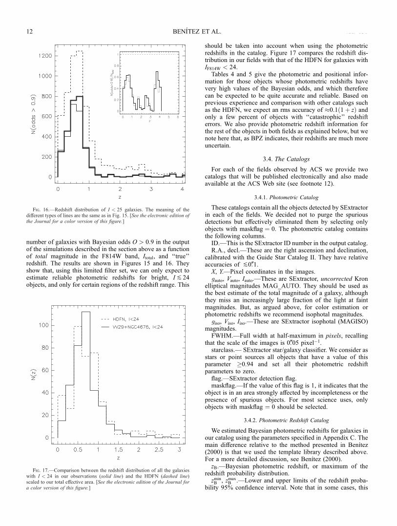
number of galaxies with Bayesian odds O > 0:9 in the outputof the simulations described in the section above as a functionof total magnitude in the F814W band, Itotal, and ‘‘true’’redshift. The results are shown in Figures 15 and 16. Theyshow that, using this limited filter set, we can only expect toestimate reliable photometric redshifts for bright, I P24objects, and only for certain regions of the redshift range. This

should be taken into account when using the photometricredshifts in the catalog. Figure 17 compares the redshift dis-tribution in our fields with that of the HDFN for galaxies withIF814W < 24.Tables 4 and 5 give the photometric and positional infor-

mation for those objects whose photometric redshifts havevery high values of the Bayesian odds, and which thereforecan be expected to be quite accurate and reliable. Based onprevious experience and comparison with other catalogs suchas the HDFN, we expect an rms accuracy of �0:1ð1þ zÞ andonly a few percent of objects with ‘‘catastrophic’’ redshifterrors. We also provide photometric redshift information forthe rest of the objects in both fields as explained below, but wenote here that, as BPZ indicates, their redshifts are much moreuncertain.

3.4. The Catalogs

For each of the fields observed by ACS we provide twocatalogs that will be published electronically and also madeavailable at the ACS Web site (see footnote 12).

3.4.1. Photometric Catalog

These catalogs contain all the objects detected by SExtractorin each of the fields. We decided not to purge the spuriousdetections but effectively eliminated them by selecting onlyobjects with maskCag ¼ 0. The photometric catalog containsthe following columns.ID.—This is the SExtractor ID number in the output catalog.R.A., decl.—These are the right ascension and declination,

calibrated with the Guide Star Catalog II. They have relativeaccuracies of P0B1.X, Y.—Pixel coordinates in the images.gauto, Vauto, Iauto.—These are SExtractor, uncorrected Kron

elliptical magnitudes MAG_AUTO. They should be used asthe best estimate of the total magnitude of a galaxy, althoughthey miss an increasingly large fraction of the light at faintmagnitudes. But, as argued above, for color estimation orphotometric redshifts we recommend isophotal magnitudes.giso, Viso, Iiso.—These are SExtractor isophotal (MAGISO)

magnitudes.FWHM.—Full width at half-maximum in pixels, recalling

that the scale of the images is 0B05 pixel�1.starclass.— SExtractor star/galaxy classifier. We consider as

stars or point sources all objects that have a value of thisparameter �0.94 and set all their photometric redshiftparameters to zero.flag.—SExtractor detection flag.maskflag.—If the value of this flag is 1, it indicates that the

object is in an area strongly affected by incompleteness or thepresence of spurious objects. For most science uses, onlyobjects with maskflag ¼ 0 should be selected.

3.4.2. Photometric Redshift Catalog

We estimated Bayesian photometric redshifts for galaxies inour catalog using the parameters specified in Appendix C. Themain difference relative to the method presented in Benıtez(2000) is that we used the template library described above.For a more detailed discussion, see Benıtez (2000).zB.—Bayesian photometric redshift, or maximum of the

redshift probability distribution.zminB , zmax

B .—Lower and upper limits of the redshift proba-bility 95% confidence interval. Note that in some cases, this

Fig. 17.—Comparison between the redshift distribution of all the galaxieswith I < 24 in our observations (solid line) and the HDFN (dashed line)scaled to our total effective area. [See the electronic edition of the Journal fora color version of this figure.]

Fig. 16.—Redshift distribution of I < 25 galaxies. The meaning of thedifferent types of lines are the same as in Fig. 15. [See the electronic edition ofthe Journal for a color version of this figure.]


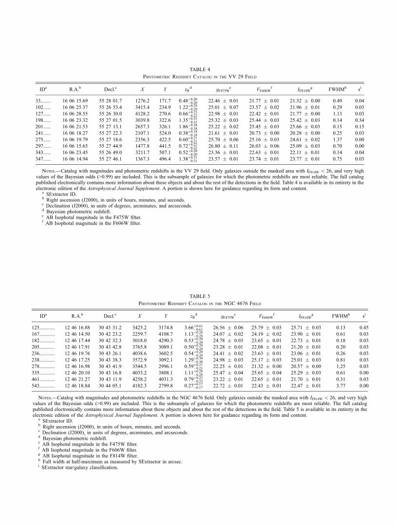
TABLE 4

Photometric Redshift Catalog in the VV 29 Field

IDa R.A.b Decl.c X Y zBd gF475W

e VF606Wf IF814W

g FWHMh si

33........ 16 06 15.69 55 28 01.7 1276.2 171.7 0:48þ0:20�0:20 22.46 � 0.01 21.77 � 0.01 21.32 � 0.00 0.49 0.04

102...... 16 06 25.37 55 26 53.4 3415.4 234.9 1:22þ0:29�0:29 25.01 � 0.07 23.57 � 0.02 21.96 � 0.01 0.29 0.03

127...... 16 06 28.55 55 26 30.0 4128.2 270.6 0:66þ0:22�0:22 22.98 � 0.01 22.42 � 0.01 21.77 � 0.00 1.13 0.03

198...... 16 06 23.32 55 27 01.5 3039.8 322.6 1:35þ0:31�0:31 25.32 � 0.03 25.44 � 0.03 25.42 � 0.03 0.14 0.34

201...... 16 06 21.53 55 27 13.1 2657.3 326.1 1:86þ0:38�0:38 25.22 � 0.02 25.45 � 0.03 25.66 � 0.03 0.15 0.15

241...... 16 06 18.27 55 27 22.3 2107.1 524.0 0:38þ0:18�0:18 21.61 � 0.01 20.73 � 0.00 20.28 � 0.00 0.25 0.03

275...... 16 06 19.79 55 27 18.6 2356.3 422.5 0:60þ0:21�0:21 25.70 � 0.06 25.16 � 0.03 24.61 � 0.02 1.37 0.00

297...... 16 06 15.65 55 27 44.9 1477.8 441.5 0:72þ0:22�0:22 26.80 � 0.11 26.03 � 0.06 25.09 � 0.03 0.70 0.00

343...... 16 06 23.45 55 26 49.0 3211.7 507.1 0:52þ0:20�0:20 23.36 � 0.01 22.63 � 0.01 22.11 � 0.01 0.14 0.04

347...... 16 06 14.94 55 27 46.1 1367.3 496.4 1:38þ0:31�0:31 23.57 � 0.01 23.74 � 0.01 23.77 � 0.01 0.75 0.03

Notes.—Catalog with magnitudes and photometric redshifts in the VV 29 field. Only galaxies outside the masked area with IF814W < 26, and very highvalues of the Bayesian odds (>0.99) are included. This is the subsample of galaxies for which the photometric redshifts are most reliable. The full catalogpublished electronically contains more information about these objects and about the rest of the detections in the field. Table 4 is available in its entirety in theelectronic edition of the Astrophysical Journal Supplement. A portion is shown here for guidance regarding its form and content.

a SExtractor ID.b Right ascension (J2000), in units of hours, minutes, and seconds.c Declination (J2000), in units of degrees, arcminutes, and arcseconds.d Bayesian photometric redshift.e AB Isophotal magnitude in the F475W filter.f AB Isophotal magnitude in the F606W filter.

TABLE 5

Photometric Redshift Catalog in the NGC 4676 Field

IDa R.A.b Decl.c X Y zBd gF475W

e VF606Wf IF814W

g FWHMh si

125............ 12 46 16.88 30 43 31.2 3425.2 3174.8 3:66þ0:61�0:61 26.56 � 0.06 25.79 � 0.03 25.71 � 0.03 0.13 0.45

167............ 12 46 14.50 30 42 23.2 2259.7 4108.7 1:13þ0:28�0:28 24.07 � 0.02 24.19 � 0.02 23.90 � 0.01 0.61 0.03

182............ 12 46 17.44 30 42 32.3 3018.0 4290.3 0:53þ0:20�0:20 24.78 � 0.03 23.65 � 0.01 22.73 � 0.01 0.18 0.03

205............ 12 46 17.91 30 43 42.8 3765.8 3089.1 0:50þ0:20�0:20 23.28 � 0.01 22.08 � 0.01 21.20 � 0.01 0.20 0.03

236............ 12 46 19.76 30 43 26.1 4038.6 3602.5 0:54þ0:20�0:20 24.41 � 0.02 23.63 � 0.01 23.06 � 0.01 0.26 0.03

238............ 12 46 17.25 30 43 38.3 3572.9 3092.1 1:29þ0:30�0:30 24.98 � 0.03 25.17 � 0.03 25.01 � 0.03 0.81 0.03

278............ 12 46 16.98 30 43 41.9 3544.5 2996.1 0:59þ0:21�0:21 22.25 � 0.01 21.32 � 0.00 20.57 � 0.00 1.25 0.03

335............ 12 46 20.10 30 43 16.8 4033.2 3808.1 1:11þ0:28�0:28 25.47 � 0.04 25.65 � 0.04 25.29 � 0.03 0.61 0.00

461............ 12 46 21.27 30 43 11.9 4258.2 4031.3 0:79þ0:23�0:23 23.22 � 0.01 22.65 � 0.01 21.70 � 0.01 0.31 0.03

543............ 12 46 18.84 30 44 05.1 4182.3 2799.8 0:27þ0:17�0:17 22.72 � 0.01 22.43 � 0.01 22.47 � 0.01 3.77 0.00

Notes.—Catalog with magnitudes and photometric redshifts in the NGC 4676 field. Only galaxies outside the masked area with IF814W < 26, and very highvalues of the Bayesian odds (>0.99) are included. This is the subsample of galaxies for which the photometric redshifts are most reliable. The full catalogpublished electronically contains more information about these objects and about the rest of the detections in the field. Table 5 is available in its entirety in theelectronic edition of the Astrophysical Journal Supplement. A portion is shown here for guidance regarding its form and content.

a SExtractor ID.b Right ascension (J2000), in units of hours, minutes, and seconds.c Declination (J2000), in units of degrees, arcminutes, and arcseconds.d Bayesian photometric redshift.e AB Isophotal magnitude in the F475W filter.f AB Isophotal magnitude in the F606W filter.g AB Isophotal magnitude in the F814W filter.h Full width at half-maximum as measured by SExtractor in arcsec.i SExtractor star/galaxy classification.

probability distribution is multimodal, so these values or zBare not very meaningful.

tB.—Bayesian spectral type. The types are El (1), Sbc(2),Scd(3), Im(4), SB3(5), and SB2(6).

odds.—Bayesian odds. This is the integral of the redshiftprobability distribution in a region of �0:2ð1þ zBÞ. If close to1, it means that the redshift probability is narrow and has asingle peak. Very low values of the odds indicate that thecolor/magnitude information is almost useless to estimate theredshift.

zML.—Maximum-likelihood redshift. We provide this toallow users to compare with the value of zB, and also to un-

derstand the effects of the prior on the redshift estimate. As anestimate of the redshift we recommend the use of zB, whichhas been proved to be more accurate and reliable.tML.—Maximum-likelihood spectral type.�2.—This is the value corresponding to the maximum-

likelihood redshift/spectral type fit.

4. NUMBER COUNTS

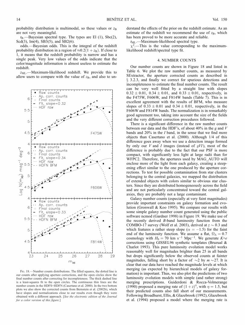
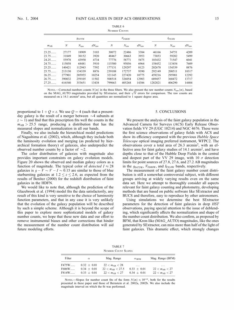
Our number counts are shown in Figure 18 and listed inTable 6. We plot the raw number counts, as measured bySExtractor, the aperture corrected counts as described inx 3.2.3, and finally we correct for spurious detections andincompleteness to estimate the final number counts. The resultcan be very well fitted by a straight line with slopes0:32 � 0:01, 0:34 � 0:01, and 0:33 � 0:01, respectively, inthe F475W, F606W, and F814W bands (Table 7). This is inexcellent agreement with the results of BFM, who measureslopes of 0:33 � 0:01 and 0:34 � 0:01, respectively, in theF606W and F814W bands. The normalization is in remarkablygood agreement too, taking into account the size of the fieldsand the very different correction procedures followed.There is a significant difference in the raw number counts

between our data and the HDF’s, of about 40% in the g and Vbands and 20% in the I band, in the sense that we find moreobjects than Casertano et al. (2000). Although 1/4 of thisdifference goes away when we use a detection image formedby only our V and I images (instead of gVI ), most of thedifference is probably due to the fact that our PSF is morecompact, with significantly less light at large radii than forWFPC2. Therefore, the apertures used by MAG_AUTO willenclose more of the light from each galaxy, creating a steep-ening effect similar to the one produced by the aperture cor-rections. To test for possible contamination from star clustersbelonging to the central galaxies, we mapped the distributionof extended objects with colors similar to obvious star clus-ters. Since they are distributed homogeneously across the fieldand are not particularly concentrated toward the central gal-axies, they are probably not a large contaminant.Galaxy number counts (especially at very faint magnitudes)

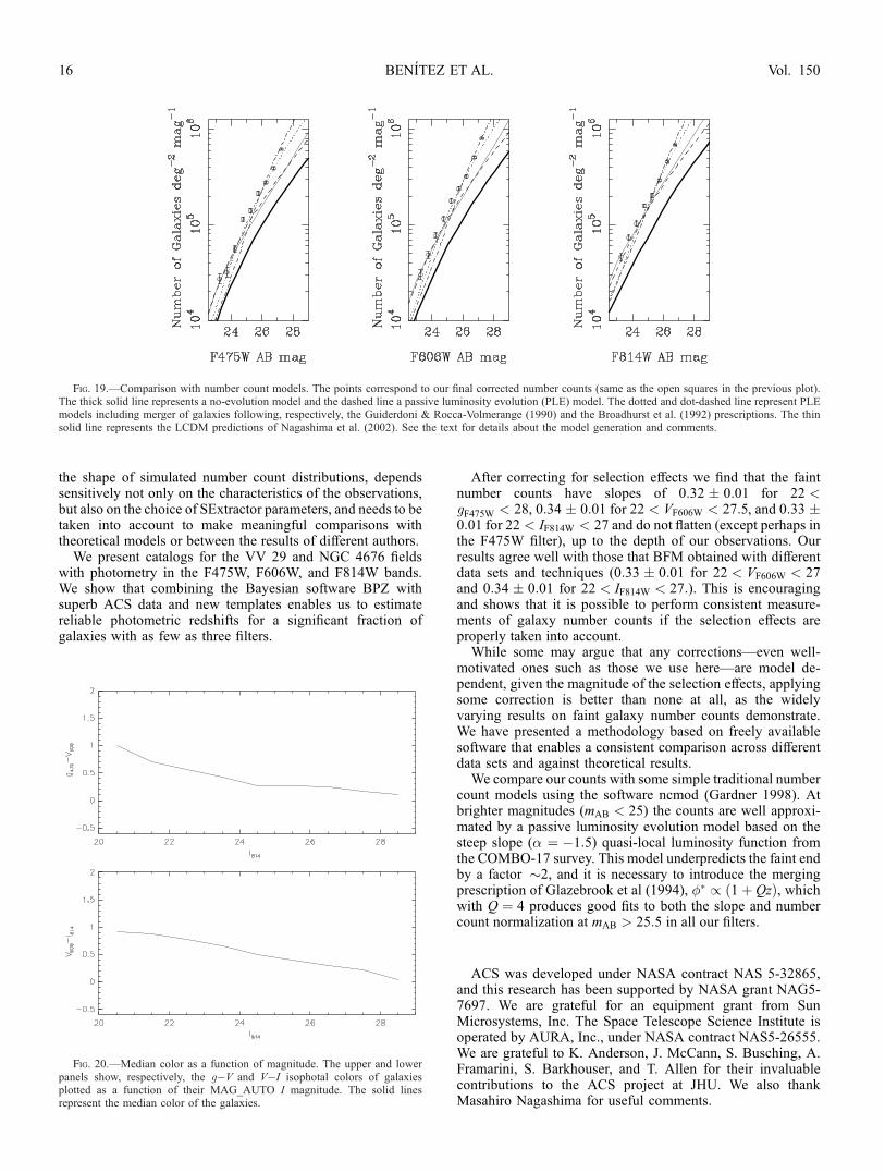
provide important constraints on galaxy formation and evo-lution (Gronwall & Koo 1995). We compare our results withsome simple galaxy number count generated using the publicsoftware ncmod (Gardner 1998) in Figure 19. We make use ofthe recently derived B-band luminosity function from theCOMBO-17 survey (Wolf et al. 2003), derived at z � 0:3 andwhich features a rather steep slope (� ¼ �1:5) for the faintend of the luminosity function. We assume a flat, �� ¼ 0:7cosmology with H0 ¼ 70 km s�1 Mpc�1. We generate K+ecorrections using GISSEL96 synthetic templates (Bruzual &Charlot 1993). This pure luminosity evolution model worksreasonably well for magnitudes brighter than 25 in all bandsbut drops significantly below the observed counts at faintermagnitudes, falling short by a factor of �2 by m �27. It isclear that our data have reached the magnitude levels at whichmerging (as expected by hierarchical models of galaxy for-mation) is important. Thus, we also plot the predictions of twoluminosity evolution models with simple (and rather strong)merging prescriptions. Guiderdoni & Rocca-Volmerange(1990) proposed a merging rate of ð1þ zÞ�, with � ¼ 1:5, buttheir predicted counts also fall short of our measurements.Following Broadhurst, Ellis, &Glazebrook (1992), Glazebrooket al. (1994) proposed a model where the merging rate is

Fig. 18.—Number counts distributions. The filled squares, the dotted line isour counts after applying aperture corrections, and the open circles show thefinal number counts after correcting for incompleteness. The thick dashed lineis a least-squares fit to the open circles. The continuous thin lines are thenumber counts in the HDFS+HDFN (Casertano et al. 2000). In the two bottomplots we also show the corrected counts from Bernstein et al. (2002b), whichhave slopes and normalizations close to our results even though they wereobtained with a different approach. [See the electronic edition of the Journalfor a color version of this figure.]


proportional to 1þ Q� z. We use Q ¼ 4 (such that a present-day galaxy is the result of a merger between �4 subunits atz � 1) and find that this prescription fits well the counts in themAB > 25:5 range, producing a distribution that has themeasured slopes and normalization in all our bands.

Finally, we also include the hierarchical model predictionsof Nagashima et al. (2002), which, although they include boththe luminosity evolution and merging (as predicted by hier-archical formation theory) of galaxies, also underpredict theobserved number counts by a factor of �2.

The color distribution of galaxies with magnitude alsoprovides important constraints on galaxy evolution models.Figure 20 shows the observed and median galaxy colors as afunction of magnitude. The typical color of detected I � 28galaxies is g � V � V � I � 0:15 are similar to those of bluestarbursting galaxies at 1:2 z 2:6, as expected from theresults of Benıtez (2000) for the redshift distribution of faintgalaxies in the HDFN.

We would like to note that, although the prediction of theGlazebrook et al. (1994) model fits the data satisfactorily, anyresult of this kind is very sensitive to the choice of luminosityfunction parameters, and that in any case it is very unlikelythat the evolution of the galaxy population will be describedby such a simple scheme. Although it is beyond the scope ofthis paper to explore more sophisticated models of galaxynumber counts, we hope that these new data and our effort toremove instrumental biases and other corrections that hinderthe measurement of the number count distribution will aidfuture modeling efforts.

5. CONCLUSIONS

We present the analysis of the faint galaxy population in theAdvanced Camera for Surveys (ACS) Early Release Obser-vation fields VV 29 (UGC 10214) and NGC 4676. These werethe first science observations of galaxy fields with ACS andshow its efficiency compared with the previous Hubble SpaceTelescope optical imaging preferred instrument, WFPC2. Theobservations cover a total area of 26.3 arcmin2, with an ef-fective area for faint galaxy studies of 14.1 arcmin2, and havedepths close to that of the Hubble Deep Fields in the centraland deepest part of the VV 29 image, with 10 � detectionlimits for point sources of 27.8, 27.6, and 27.2 AB magnitudesin the gF475W, VF606W, and IF814W bands, respectively.

The measurement of the faint galaxy number count distri-bution is still a somewhat controversial subject, with differentgroups arriving at widely varying results even on the samedata set. Here we attempt to thoroughly consider all aspectsrelevant for faint galaxy counting and photometry, developingmethods that are based on public software like SExtractor andBUCS and therefore, easy to reproduce by other astronomers.

Using simulations we determine the best SExtractorparameters for the detection of faint galaxies in deep HSTobservations, paying special attention to the issue of deblend-ing, which significantly affects the normalization and shape ofthe number count distribution. We also confirm, as proposed byBFM, that Kron-like (MAG_AUTO) magnitudes, like the onesgenerated by SExtractor, can miss more than half of the light offaint galaxies. This dramatic effect, which strongly changes

TABLE 6

Number Counts

gF475W VF606W IF814W

mAB N Nraw dNraw N Nraw dNraw N Nraw dNraw

23.25....... 27177 18909 3103 30072 22486 3384 46166 34751 4209

23.75....... 31849 30152 3920 48467 30663 3953 73853 59282 5499

24.25....... 55978 43950 4734 77776 58771 5475 103432 71547 6041

24.75....... 115058 68481 5910 115580 95056 6964 158452 113454 7609

25.25....... 140421 112943 7592 177131 129297 8123 202678 154339 8876

25.75....... 213130 154339 8876 239108 172737 9390 292149 208511 10317

26.25....... 277901 205955 10254 321145 227420 10775 459216 295901 12292

26.75....... 390832 259105 11502 508518 326054 12903 689457 368472 13717

27.25....... 616540 353651 13438 799663 405268 14386 1282821 406290 14404

Notes.—Corrected numbers counts NðmÞ in the three filters. We also present the raw number counts NrawðmÞ, basedon the MAG_AUTO magnitudes provided by SExtractor, and their

ffiffiffiffiN

perrors for comparison. The raw counts are

measured on a 14.1 arcmin2 area, but all quantities are normalized to 1 square degree area.

TABLE 7

Number Count Slopes

Filter � Mag. Range �BFM Mag. Range (BFM)

F475W...... 0.32 � 0.01 22 < mAB < 28 . . . . . .

F606W...... 0.34 � 0.01 22 < mAB < 27:5 0.33 � 0.01 22 < mAB < 27

F814W...... 0.33 � 0.01 22 < mAB < 27 0.34 � 0.01 22 < mAB < 27

Notes.—Slopes for number count fits of the form NðmÞ / 10�m, both for the resultspresented in these paper and those of Bernstein et al. 2002a, 2002b. We also include themagnitude interval on which the fit was performed.


the shape of simulated number count distributions, dependssensitively not only on the characteristics of the observations,but also on the choice of SExtractor parameters, and needs to betaken into account to make meaningful comparisons withtheoretical models or between the results of different authors.

We present catalogs for the VV 29 and NGC 4676 fieldswith photometry in the F475W, F606W, and F814W bands.We show that combining the Bayesian software BPZ withsuperb ACS data and new templates enables us to estimatereliable photometric redshifts for a significant fraction ofgalaxies with as few as three filters.

After correcting for selection effects we find that the faintnumber counts have slopes of 0:32 � 0:01 for 22 <gF475W < 28, 0:34 � 0:01 for 22 < VF606W < 27:5, and 0:33 �0:01 for 22 < IF814W < 27 and do not flatten (except perhaps inthe F475W filter), up to the depth of our observations. Ourresults agree well with those that BFM obtained with differentdata sets and techniques (0:33 � 0:01 for 22 < VF606W < 27and 0:34 � 0:01 for 22 < IF814W < 27:). This is encouragingand shows that it is possible to perform consistent measure-ments of galaxy number counts if the selection effects areproperly taken into account.While some may argue that any corrections—even well-

motivated ones such as those we use here—are model de-pendent, given the magnitude of the selection effects, applyingsome correction is better than none at all, as the widelyvarying results on faint galaxy number counts demonstrate.We have presented a methodology based on freely availablesoftware that enables a consistent comparison across differentdata sets and against theoretical results.We compare our counts with some simple traditional number

count models using the software ncmod (Gardner 1998). Atbrighter magnitudes (mAB < 25) the counts are well approxi-mated by a passive luminosity evolution model based on thesteep slope (� ¼ �1:5) quasi-local luminosity function fromthe COMBO-17 survey. This model underpredicts the faint endby a factor �2, and it is necessary to introduce the mergingprescription of Glazebrook et al (1994), �� / ð1þ QzÞ, whichwith Q ¼ 4 produces good fits to both the slope and numbercount normalization at mAB > 25:5 in all our filters.

ACS was developed under NASA contract NAS 5-32865,and this research has been supported by NASA grant NAG5-7697. We are grateful for an equipment grant from SunMicrosystems, Inc. The Space Telescope Science Institute isoperated by AURA, Inc., under NASA contract NAS5-26555.We are grateful to K. Anderson, J. McCann, S. Busching, A.Framarini, S. Barkhouser, and T. Allen for their invaluablecontributions to the ACS project at JHU. We also thankMasahiro Nagashima for useful comments.

Fig. 19.—Comparison with number count models. The points correspond to our final corrected number counts (same as the open squares in the previous plot).The thick solid line represents a no-evolution model and the dashed line a passive luminosity evolution (PLE) model. The dotted and dot-dashed line represent PLEmodels including merger of galaxies following, respectively, the Guiderdoni & Rocca-Volmerange (1990) and the Broadhurst et al. (1992) prescriptions. The thinsolid line represents the LCDM predictions of Nagashima et al. (2002). See the text for details about the model generation and comments.

Fig. 20.—Median color as a function of magnitude. The upper and lowerpanels show, respectively, the g�V and V�I isophotal colors of galaxiesplotted as a function of their MAG_AUTO I magnitude. The solid linesrepresent the median color of the galaxies.


APPENDIX A

BUCS SIMULATIONS

A robust, model-independent way of generating realistic galaxy fields is to take deep observations already available and thenrearrange the objects to generate another field. Using this approach, we simulate deep ACS images with the BUCS (BouwensUniverse Construction Set) software. In the first step, we determine the number of times each object appears in a given image bydrawing from a Poisson distribution with mean �objAsim, where �obj is the surface density of the object and Asim is the field areabeing simulated. In the second step, we distribute the objects across the field assuming a uniform random distribution, i.e., nospatial clustering. In the third step, we simulate ACS images in any number of filters using the Monte Carlo catalogs generated inthe first two steps. We place objects in these images in one of two ways: using their best-fit analytic profiles or resampling theoriginal objects onto the image. To do this properly, BUCS (1) k-corrects each object template using best-fit pixel-by-pixel andobject SED and (2) corrects its PSF to match the PSF for the ACS filter being simulated. Finally, we add the expected amount ofnoise to the image. The formalism used to perform these final two steps is described more extensively in Bouwens et al. (2003) andBouwens (2004).

Since these simulations are just a rearrangement of objects from an input field, they should be an extremely accurate repre-sentation of the observations, not only in number, angular size, ellipticity distributions, and color distributions, but also inmorphology and pixel-by-pixel color variations.

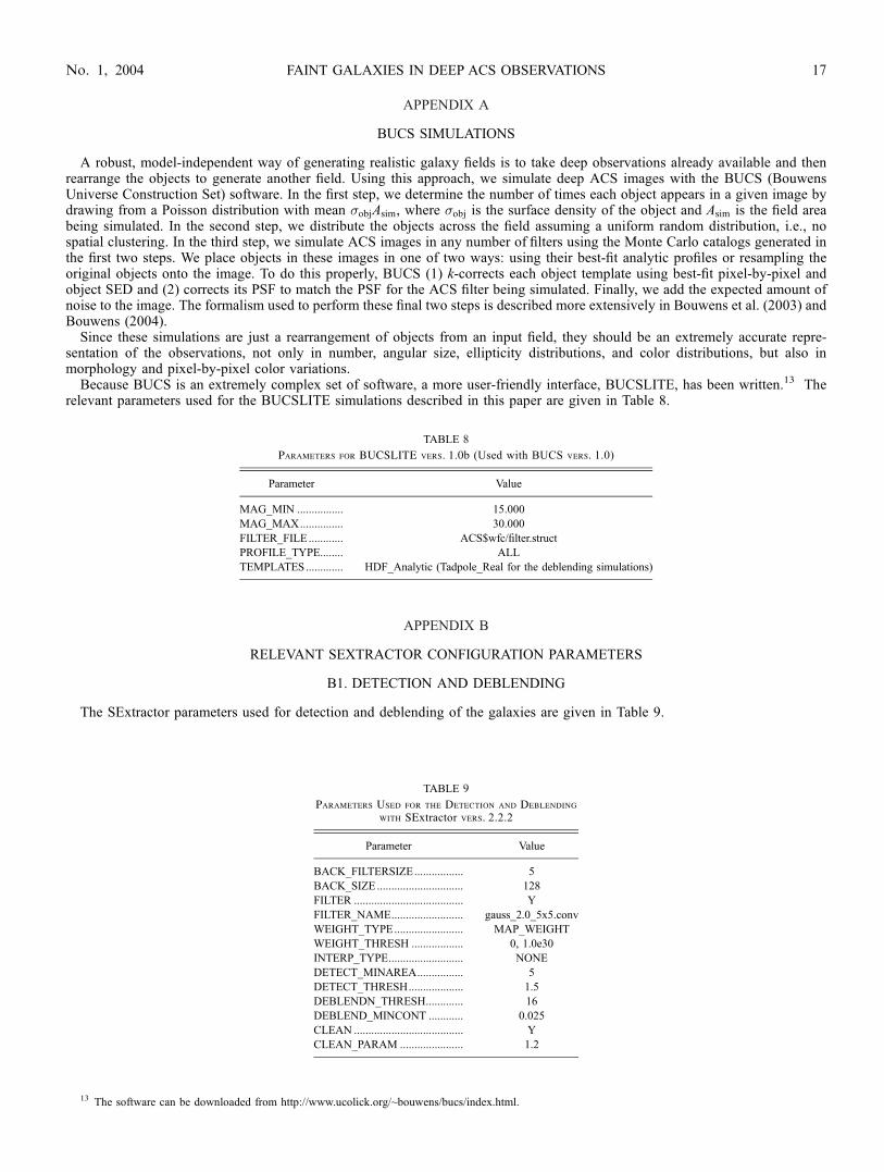
Because BUCS is an extremely complex set of software, a more user-friendly interface, BUCSLITE, has been written.13 Therelevant parameters used for the BUCSLITE simulations described in this paper are given in Table 8.

APPENDIX B

RELEVANT SEXTRACTOR CONFIGURATION PARAMETERS

B1. DETECTION AND DEBLENDING

The SExtractor parameters used for detection and deblending of the galaxies are given in Table 9.

TABLE 8

Parameters for BUCSLITE vers. 1.0b (Used with BUCS vers. 1.0)

Parameter Value

MAG_MIN ................ 15.000

MAG_MAX............... 30.000

FILTER_FILE ............ ACS$wfc/filter.struct

PROFILE_TYPE........ ALL

TEMPLATES............. HDF_Analytic (Tadpole_Real for the deblending simulations)

TABLE 9

Parameters Used for the Detection and Deblending

with SExtractor vers. 2.2.2

Parameter Value

BACK_FILTERSIZE................. 5

BACK_SIZE .............................. 128

FILTER ...................................... Y

FILTER_NAME......................... gauss_2.0_5x5.conv

WEIGHT_TYPE........................ MAP_WEIGHT

WEIGHT_THRESH .................. 0, 1.0e30

INTERP_TYPE.......................... NONE

DETECT_MINAREA................ 5

DETECT_THRESH................... 1.5

DEBLENDN_THRESH............. 16

DEBLEND_MINCONT ............ 0.025

CLEAN ...................................... Y

CLEAN_PARAM ...................... 1.2

13 The software can be downloaded from http://www.ucolick.org/~bouwens/bucs/index.html.


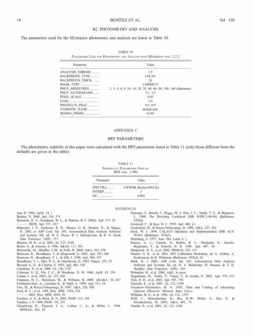
B2. PHOTOMETRY AND ANALYSIS

The parameters used for the SExtractor photometry and analysis are listed in Table 10.

APPENDIX C

BPZ PARAMETERS

The photometric redshifts in this paper were calculated with the BPZ parameters listed in Table 11 (only those different from thedefaults are given in the table).

REFERENCES

Arp, H. 1966, ApJS, 14, 1Benıtez, N. 2000, ApJ, 536, 571Bernstein, R. A., Freedman, W. L., & Madore, B. F. 2002a, ApJ, 571, 56———. 2002b, ApJ, 571, 107Blakeslee, J. P., Anderson, K. R., Meurer, G. R., Benıtez, N., & Magee,D. 2003, in ASP Conf. Ser. 295, Astronomical Data Analysis Softwareand Systems XII, ed. H. E. Payne, R. I. Jedrzejewski, & R. N. Hook(San Francisco: ASP), 257

Blanton, M. R., et al. 2003, AJ, 125, 2348Bertin, E., & Arnouts, S. 1996, A&AS, 117, 393Bolzonella, M., Miralles, J.-M., & Pello, R. 2000, A&A, 363, 476Bouwens, R., Broadhurst, T., & Illingworth, G. 2003, ApJ, 593, 640Bouwens, R., Broadhurst, T. J., & Silk, J. 1998, ApJ, 506, 557Broadhurst, T. J., Ellis, R. S., & Glazebrook, K. 1992, Nature, 355, 55Bruzual A., G., & Charlot, S. 1993, ApJ, 405, 538Casertano, S., et al. 2000, AJ, 120, 2747Coleman, G. D., Wu, C.-C., & Weedman, D. W. 1980, ApJS, 43, 393Csabai, I., et al. 2003, AJ, 125, 580Ferguson, H. C., Dickinson, M., & Williams, R. 2000, ARA&A, 38, 667Fernandez-Soto, A., Lanzetta, K., & Yahil, A. 1999, ApJ, 513, 34Fioc, M., & Rocca-Volmerange, B. 1997, A&A, 326, 950Ford, H. C., et al. 1998, Proc. SPIE, 3356, 234———. 2002, Proc. SPIE, 4854, 81Fruchter, A. S., & Hook, R. N. 2002, PASP, 114, 144Gardner, J. P. 1998, PASP, 110, 291Glazebrook, K., Peacock, J. A., Collins, C. A., & Miller, L. 1994,MNRAS, 266, 65

Gonzaga, S., Biretta, J., Wiggs, M. S. Hsu, J. C., Smith, T. E., & Bergeron,L. 1998, The Drizzling Cookbook (ISR WFPC2-98-04) (Baltimore:STScI)

Gronwall, C., & Koo, D. C. 1995, ApJ, 440, L1Guiderdoni, B., & Rocca-Volmerange, B. 1990, A&A, 227, 362Hack, W. J. 1999, CALACS Operation and Implementation (ISR ACS-99-03) (Baltimore: STScI)

Holmberg, E. 1937, Ann. Obs. Lund, 6, 1Kinney, A. L., Calzetti, D., Bohlin, R. C., McQuade, K., Storchi-Bergmann, T., & Schmitt, H. R. 1996, ApJ, 467, 38

Madgwick, D. S., et al. 2002, MNRAS, 333, 133Meurer, G. R., et al. 2003, HST Calibration Workshop, ed. S. Arribas, A.Koekemoer, & B. Whitmore (Baltimore: STScI), 65

Mink, D. J. 2002, ASP Conf. Ser. 281, Astronomical Data AnalysisSoftware and Systems XI, ed. D. A. Bohlender, D. Durand, & T. H.Handley (San Francisco: ASP), 169

Mobasher, B., et al. 2004, ApJL, in pressNagashima, M., Yoshii, Y., Totani, T., & Gouda, N. 2002, ApJ, 578, 675Tran, H. D., et al. 2003, ApJ, 585, 750Vanzella, E., et al. 2001, AJ, 122, 2190Vorontsov-Velyaminov, B. A. 1959, Atlas and Catalog of InteractingGalaxies (Moscow: Moscow State Univ.)

Williams, R. E., et al. 1996, AJ, 112, 1335Wolf, C., Meisenheimer, K., Rix, H.-W., Borch, A., Dye, S., &Kleinheinrich, M. 2003, A&A, 401, 73

Yasuda, N., et al. 2001, AJ, 122, 1104

TABLE 10

Parameters Used for Photometry and Analysis with SExtractor vers. 2.2.2

Parameter Value

ANALYSIS_THRESH........... 1.5

BACKPHOTO_TYPE ........... LOCAL

BACKPHOTO_THICK ......... 26

MASK_TYPE ........................ CORRECT

PHOT_APERTURES............. 2, 3, 4, 6, 8, 10, 14, 20, 28, 40, 60, 80, 100, 160 (diameters)

PHOT_AUTOPARAMS ........ 2.5, 3.3

PIXEL_SCALE...................... 0.05

GAIN...................................... 1.0

PHOTFLUX_FRAC .............. 0.5, 0.9

STARNNW_NAME .............. default.nnw

SEEING_FWHM................... 0.105

TABLE 11

Nondefault Parameters Used by

BPZ vers. 1.98b

Parameter Value

SPECTRA....... CWWSB_Benitez2003.list

INTERP........... 2

DZ ................... 0.002


Faint Galaxies in Deep Advanced Camera for Surveys Observations

Documents