Failure Assessment Diagram Analysis of Creep … Assessment Diagram Analysis of Creep Crack Initiation in 316H Stainless Steel C. M. Davies*, N. P. O’Dowd, D. W. Dean †, K. M.

Failure Assessment Diagram Analysis of Creep Crack Initiation in 316H Stainless Steel

C. M. Davies*, N. P. O’Dowd, D. W. Dean†, K. M. Nikbin, R. A. Ainsworth†

Department of Mechanical Engineering, Imperial College London, South Kensington

Campus, London SW7 2AZ, UK †British Energy plc, Barnett Way, Barnwood, Gloucester GL4 3RS, UK.

Abstract

In this work the time dependent failure assessment diagram (TDFAD) approach is applied to the study of crack initiation in Type 316H stainless steel, a material commonly used in high temperature applications. A TDFAD has been constructed for the steel at a temperature of 550oC, and was found to be relatively insensitive to time. The TDFAD procedure is then applied to predict initiation times, at increments of creep crack growth Δa = 0.2 mm and Δa = 0.5 mm, for tests on compact tension specimens and the results compared to experimentally determined values. It has been found that initiation time predictions are sensitive to the creep toughness values, and to the limit load (or reference stress) solution used. Conservative predictions of initiation times have been achieved through the use of the lower bound creep toughness values in conjunction with the plane strain limit load solution. The plane stress limit load solution has given conservative predictions for all bounds of creep toughness used. Keywords: Failure assessment diagram, creep crack initiation, stainless steel

* Corresponding author. E-mail address: [email protected]

1 Introduction

The failure assessment diagram (FAD) approach has been widely used to assess the safety of

defects in engineering components, e.g. [1]. The time dependent failure assessment diagram

(TDFAD), [2], an extended form of the FAD, has recently been developed in order to

accommodate the high temperature creep regime within an FAD-based approach. The use of

a TDFAD has many advantages—detailed calculations of crack tip parameters such as C* are

not needed; it is not necessary to establish the fracture regime in advance and the TDFAD

can indicate whether failure is controlled by crack growth in the small-scale or widespread

creep regime or by creep rupture.

The TDFAD procedure is generally used to determine whether a specified crack extension

will be achieved within the assessment time. It may also be used to determine the time

required for a limited crack extension to occur. Hence approximate initiation times can be

obtained, using an engineering definition of initiation, generally taken to be the time for a

defined amount of crack extension (typically 0.2 and 0.5 mm), [3]. The procedure is currently

limited to cracks under Mode I loading and to the initiation of cracking or crack extensions

that are small compared to the defect and component dimensions.

In this work experimental creep crack growth (CCG) test data from [4] for an austenitic Type

316H stainless steel at 550oC, have been analysed. The dependence of the creep toughness

on time has been determined from these data. TDFADs have been constructed for the

material under study and calculations carried out on a selected test to assess the conservatism

of the TDFAD approach in the prediction of creep crack initiation. The sensitivity of the

creep initiation predictions to the scatter in and to the limit load (reference stress)

solution used is also examined.

cmatK

cmatK

2 Review of the Time Dependent Failure Assessment Diagram (TDFAD) Approach

2.1 TDFAD Parameters

The procedures and parameters used in a TDFAD analysis are similar to that of the R6

Option 2 FAD [1] except that fracture toughness is replaced by creep toughness, to be

defined later, and time dependent stress and strain parameters are required. In the TDFAD,

for the case of a single primary load, the parameters Kr and Lr are defined as follows:

Page 2 of 26

cmat

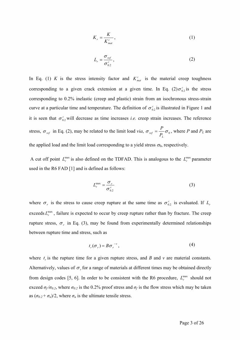
r KKK = , (1)

cref

rL2.0σ

σ= , (2)

In Eq. (1) K is the stress intensity factor and is the material creep toughness

corresponding to a given crack extension at a given time. In Eq.

cmatK

(2) c2.0σ is the stress

corresponding to 0.2% inelastic (creep and plastic) strain from an isochronous stress-strain

curve at a particular time and temperature. The definition of is illustrated in c2.0σ Figure 1 and

it is seen that will decrease as time increases i.e. creep strain increases. The reference

stress,

c2.0σ

refσ in Eq. (2), may be related to the limit load via, 0σσL

ref PP

= , where P and PL are

the applied load and the limit load corresponding to a yield stress σ0, respectively.

A cut off point is also defined on the TDFAD. This is analogous to the parameter

used in the R6 FAD [1] and is defined as follows:

maxrL max

rL

cr

rL2.0

max

σσ

= (3)

where rσ is the stress to cause creep rupture at the same time as is evaluated. If

exceeds , failure is expected to occur by creep rupture rather than by fracture. The creep

rupture stress,

c2.0σ rL

maxrL

rσ in Eq. (3), may be found from experimentally determined relationships

between rupture time and stress, such as

vrrr Bt −= σσ )( , (4)

where is the rupture time for a given rupture stress, and B and v are material constants.

Alternatively, values of

rt

rσ for a range of materials at different times may be obtained directly

from design codes [5, 6]. In order to be consistent with the R6 procedure, should not

exceed σ

maxrL

f /σ0.2, where σ0.2 is the 0.2% proof stress and σf is the flow stress which may be taken

as (σ0.2 + σu)/2, where σu is the ultimate tensile stress.

Page 3 of 26

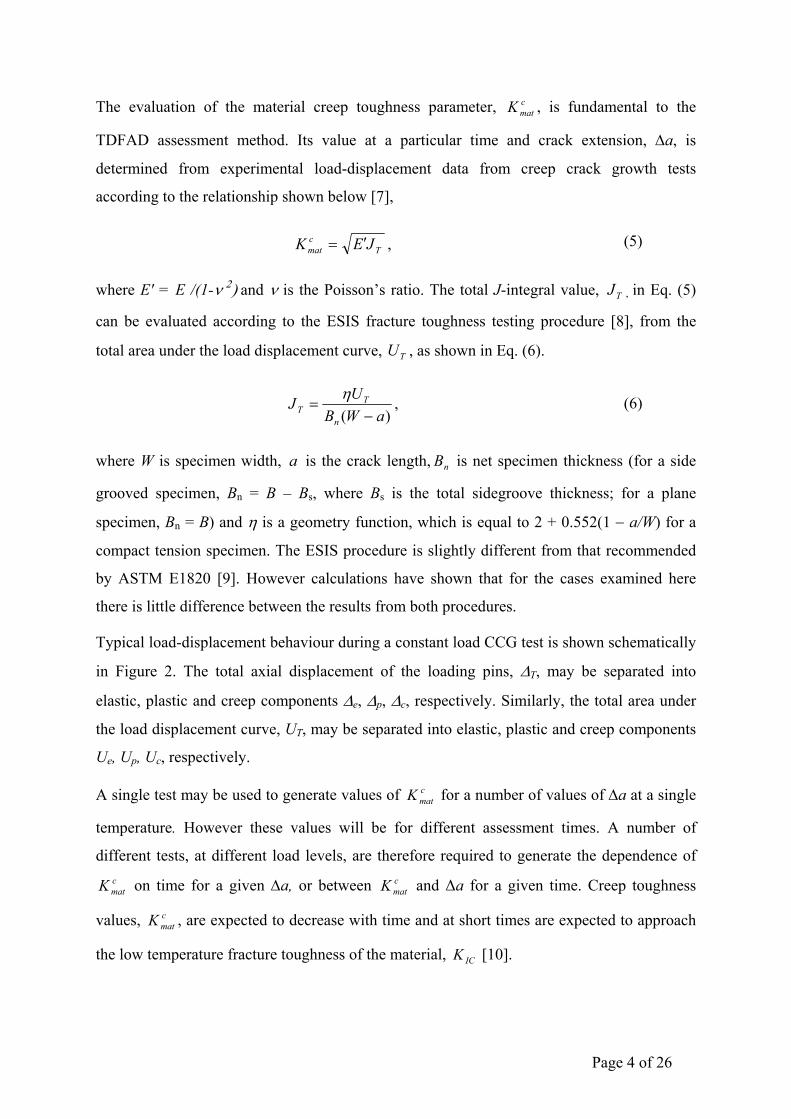
The evaluation of the material creep toughness parameter, , is fundamental to the

TDFAD assessment method. Its value at a particular time and crack extension, Δa, is

determined from experimental load-displacement data from creep crack growth tests

according to the relationship shown below [7],

cmatK

Tcmat JEK ′= , (5)

where E′ = E /(1-ν 2) and ν is the Poisson’s ratio. The total J-integral value, TJ , in Eq. (5)

can be evaluated according to the ESIS fracture toughness testing procedure [8], from the

total area under the load displacement curve, , as shown in Eq. TU (6).

)( aWBUJ

n

TT −

=η , (6)

where W is specimen width, is the crack length, is net specimen thickness (for a side

grooved specimen, B

a nB

Bn = B – BsB , where BBs is the total sidegroove thickness; for a plane

specimen, BnB = B) and η is a geometry function, which is equal to 2 + 0.552(1 − a/W) for a

compact tension specimen. The ESIS procedure is slightly different from that recommended

by ASTM E1820 [9]. However calculations have shown that for the cases examined here

there is little difference between the results from both procedures.

Typical load-displacement behaviour during a constant load CCG test is shown schematically

in Figure 2. The total axial displacement of the loading pins, ΔT, may be separated into

elastic, plastic and creep components Δe, Δp, Δc, respectively. Similarly, the total area under

the load displacement curve, UT, may be separated into elastic, plastic and creep components

Ue, Up, Uc, respectively.

A single test may be used to generate values of for a number of values of Δa at a single

temperature. However these values will be for different assessment times. A number of

different tests, at different load levels, are therefore required to generate the dependence of

on time for a given Δa, or between and Δa for a given time. Creep toughness

values, , are expected to decrease with time and at short times are expected to approach

the low temperature fracture toughness of the material, [10].

cmatK

cmatK c

matK

cmatK

ICK

Page 4 of 26

2.2 Isochronous Stress-Strain Curves

Isochronous stress-strain curves for the specified temperature are required for each time of

interest in order to determine the 0.2% inelastic strain, , and the overall TDFAD. The

schematic diagram in

c2.0σ

Figure 1 shows how and are determined. If sufficient

experimental data is not available, theoretical isochronous stress-strain curves can be

constructed from the summation of equations which specify the dependence of elastic, plastic

and creep strains on stress for the given material and temperature. Isochronous stress-strain

curves can also be obtained from design codes [5, 6].

c2.0σ 2.0σ

2.3 Formation and Application of TDFAD

A failure assessment diagram for a specific time is defined by the equations:

21

2.03

2.0 2

−

⎥⎥⎦

⎤

⎢⎢⎣

⎡+=

ref

cr

cr

refr E

LLE

Kεσ

σε

when maxrr LL ≤ (7)

0=rK when . maxrr LL > (8)

In Eq. (7) E is Young’s modulus and refε is the total strain corresponding to the reference

stress from the isochronous stress-strain curve at the particular time and temperature (see

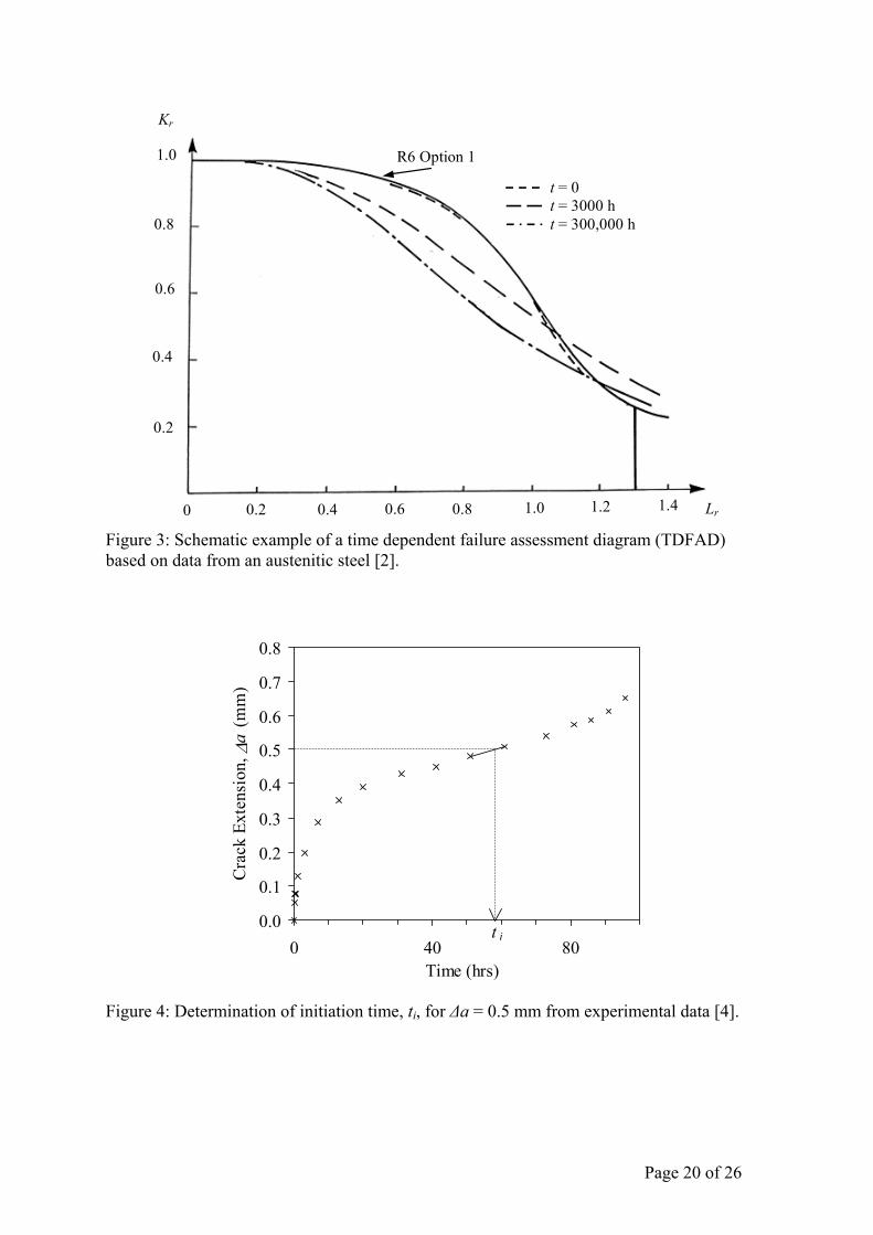
Figure 1). An example of a TDFAD is shown in Figure 3, which is based on isochronous data

for an austenitic steel at 600oC at times of 0, 3000 and 300,000 hours [2].

The TDFAD can be used to predict (i) if a crack will extend a distance Δa in a given time or

(ii) the time required for a specified amount of crack extension. Since the engineering

definition of creep crack initiation is the period of time required for an increment of crack

growth Δa, the TDFAD may be used to predict initiation times. For many materials the

curves do not vary greatly with time and curves for longer times can be used to provide a

conservative TDFAD for an assessment at shorter times.

The following steps describe the TDFAD assessment procedure [2]:

(i) Specify component and defect geometry, loading conditions, temperature, etc.

(ii) Define the maximum tolerable crack extension, or if predicting initiation times

specify the initiation distance, Δa.

Page 5 of 26

(iii) Obtain uniaxial creep data for specified times at the operating temperature (i.e.

, ). rσ c2.0σ

(iv) Construct the TDFAD for each time of interest, using Eq. (7) and the

isochronous stress-strain curves.

(v) Determine values of material creep toughness, , for each time of interest

for the specified maximum tolerable crack extension / initiation distance, Δa.

cmatK

(vi) Calculate values of Lr and Kr at the current value of crack length, a. In

initiation time assessments the initial crack length, a0, is the appropriate value

to use. (The crack extension at initiation Δa << a0, so that changes in crack size

have a negligible effect on these calculations.)

(vii) Plot the point (Lr , Kr) on the TDFAD. If the point lies within the FAD then the

crack extension is less than Δa and creep rupture is avoided in the assessment

time. Alternatively, to determine an initiation time, ti, a time locus of points

(Lr, Kr) is constructed, obtained for a single value of crack length, a0, at various

times. The time for a crack extension Δa is given by the intersection of this

locus with the failure assessment curve for the corresponding time.

If the TDFAD is not significantly dependent on time, estimates of initiation times may be

made from a curve evaluated at a single time or even from an R6 Option 1 curve. An iterative

process can then be implemented in order to refine the estimate, which involves the

construction of failure assessment curves for other times [2].

3 Calculation Methodology for Stainless Steel Data

Experimental creep crack growth (CCG) test data from for an austenitic Type 316H stainless

steel at 550oC have been analysed (see [4] for full details of the material specification). The

material had been taken from an ex-service superheater header removed from a power station

that had previously been in service for 76,000 hours at 520°C under a relatively low service

load. Data from a total of fourteen creep crack growth tests on compact tension (CT)

specimens of three different dimensions, large (L), standard (S) and half-size (HS), (see [4,

11]) have been analysed. Typical dimensions of these specimens are given in Table 1. The

specimens were typically side-grooved by 20 or 40 % such that BBn = 0.8B or Bn = 0.6B

respectively. Starter cracks had been cut into the specimens using a wire notch eroder.

Page 6 of 26

Constant load tests were carried out at a uniform temperature of 550 C and the applied loads

were chosen to give test durations between 500 and 1,500 hours. The amount of crack growth

was monitored using a direct current (DC) potential drop technique [3].

o

3.1 Determination of Initiation Times

The time for 0.2 mm crack extension during the CCG tests of 316H at 550oC has been

determined by linearly interpolating between the test times of two consecutively recorded

data points where Δa ≤ 0.2 mm and Δa ≥ 0.2 mm respectively. The time to achieve 0.5 mm of

crack growth has been determined similarly. The crack extension, Δa, vs. time data for one of

these tests on a standard sized specimen is shown in Figure 4, indicating the method used to

determine the initiation time for a crack extension of 0.5 mm.

3.2 Evaluating Creep Toughness Values, cmatK

As discussed in section 2.1, the value of is obtained from the area under the load

displacement curve up to crack initiation (see Eq.

cmatK

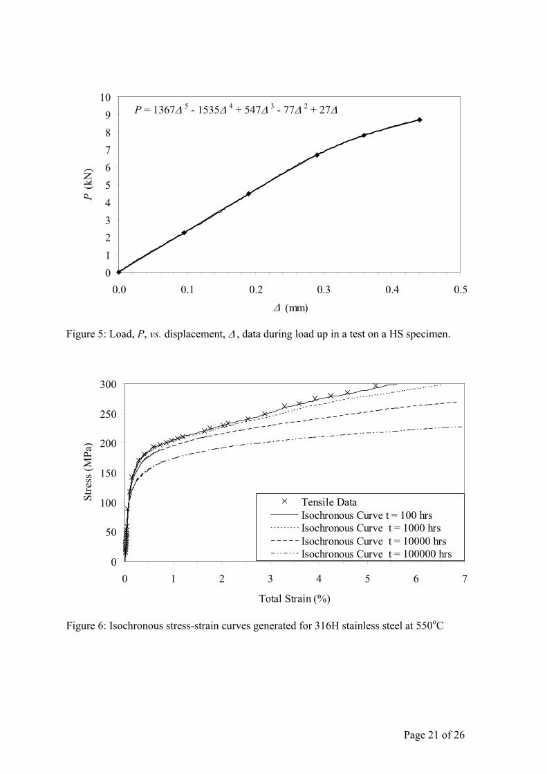
(6)). To determine this area a polynomial

equation has been fitted to the load-displacement data during load up of the CCG test, and the

integration of this equation gives the area under the loading part of the load displacement

curve, (UL = Ue + Up). A typical polynomial fit is shown in Figure 5 using data from a test on

a half size (HS) specimen, which exhibits initial linear behaviour and, at the higher load

levels, non-linear behaviour is seen due to plasticity effects. The total area under the load

displacement curve at any time, UT, is then given by the summation of the area under the

loading part of the curve (UL) and the product of the total applied load in the CCG test (which

is a constant value) and the increase in axial displacement of the loading pins, i.e.

UT = UL + PΔc (9)

Equations (5), (6) and (9) have been employed in order to determine the values of for

each set of data points measured at specific times during a CCG test. Values of for a

crack extension Δa, for example Δa = 0.2 mm, have been determined by linearly interpolating

between the values of at two consecutively recorded data points where Δa ≤ 0.2 mm

and Δa ≥ 0.2 mm, respectively.

cmatK

cmatK

cmatK

Page 7 of 26

3.3 Reference Stress Solutions

When calculating Lr, a reference stress solution, representing either plane strain (PE) or plane

stress (PS) conditions may be used. A general definition of the reference stress solution for a

CT specimen may be described by:

refeff

PmB W

σ = ’ (10)

where P is the load applied to the specimen, W is the specimen width, m is a geometric

function which varies under conditions of plane stress and plane strain, and BBeff is the

effective thickness of the specimen which is determined from [12]

2 neff n

BB BB

⎛ ⎞= −⎜ ⎟⎝ ⎠

’ (11)

The value of m for the CT specimen using the von Mises solution is [13],

( )2

1 1 1a amW W

λ γ γ γ⎡ ⎤⎧ ⎫⎪ ⎪⎛ ⎞ ⎛ ⎞⎢ ⎥= − + + + +⎨ ⎬⎜ ⎟ ⎜ ⎟⎢ ⎥⎝ ⎠ ⎝ ⎠⎪ ⎪⎩ ⎭⎣ ⎦

, (12)

1

32 plane stress where, λ = { 32

; γ = {

1 plane strain

For a given a/W the value of m is lower under plane stress conditions than plane strain,

resulting in higher values of Lr in plane stress for the same applied load, (for a typical CT

specimen examined here the plane stress reference stress is about 45% higher than the plane

strain value). Assessments made using the plane stress solution will thus generally give a

more conservative result than that obtained using the plane strain solution.

3.4 Time Dependent Stress-Strain Data

Isochronous stress-strain data have been generated using the elastic, elastic-plastic and creep

material response. The method used follows the procedure in the RCC-MR design code [14]

for primary-secondary creep of Type 316 stainless steel material. Thus, the primary and

secondary creep strain increments, cpεΔ and c

sεΔ , are calculated according to:

Page 8 of 26

/1/ (1 1/ )pn pc p pp pp A tε σ ε −Δ = Δ ,

c ns A tε σΔ = Δ .

(13)

The creep strain increment, Δε c, is equal to the larger of the two increments calculated from

Eq. (13) i.e.

cpεΔ{ for ≥ c

pεΔ csεΔ

Δε c =

csεΔ for < c

pεΔ csεΔ

(14)

The primary and secondary creep constants in Eq. (13) are p = 0.746, Ap = 2.60 × 10-23,

np = 7.45, A = 1.559 × 10-35 and n = 11.95 (for stress in MPa), which were obtained by

fitting to uniaxial creep data over a range of conditions [4].

For a particular time, the total strain at any stress level is given by the sum of the elastic and

plastic strain and the total creep strain accumulated in that time:

( ) ( ) ( ) ( ),total e pl c

t

t tε σ ε σ ε σ ε σ= + + Δ , Δ∑ . (15)

There were insufficient tensile data in [4] which could be used to provide the elastic-plastic

response of the material in Eq. (15) . Therefore data were obtained from material of the same

cast, which had been exposed to similar, but not identical, service conditions to that of the

test specimens analysed here [4].

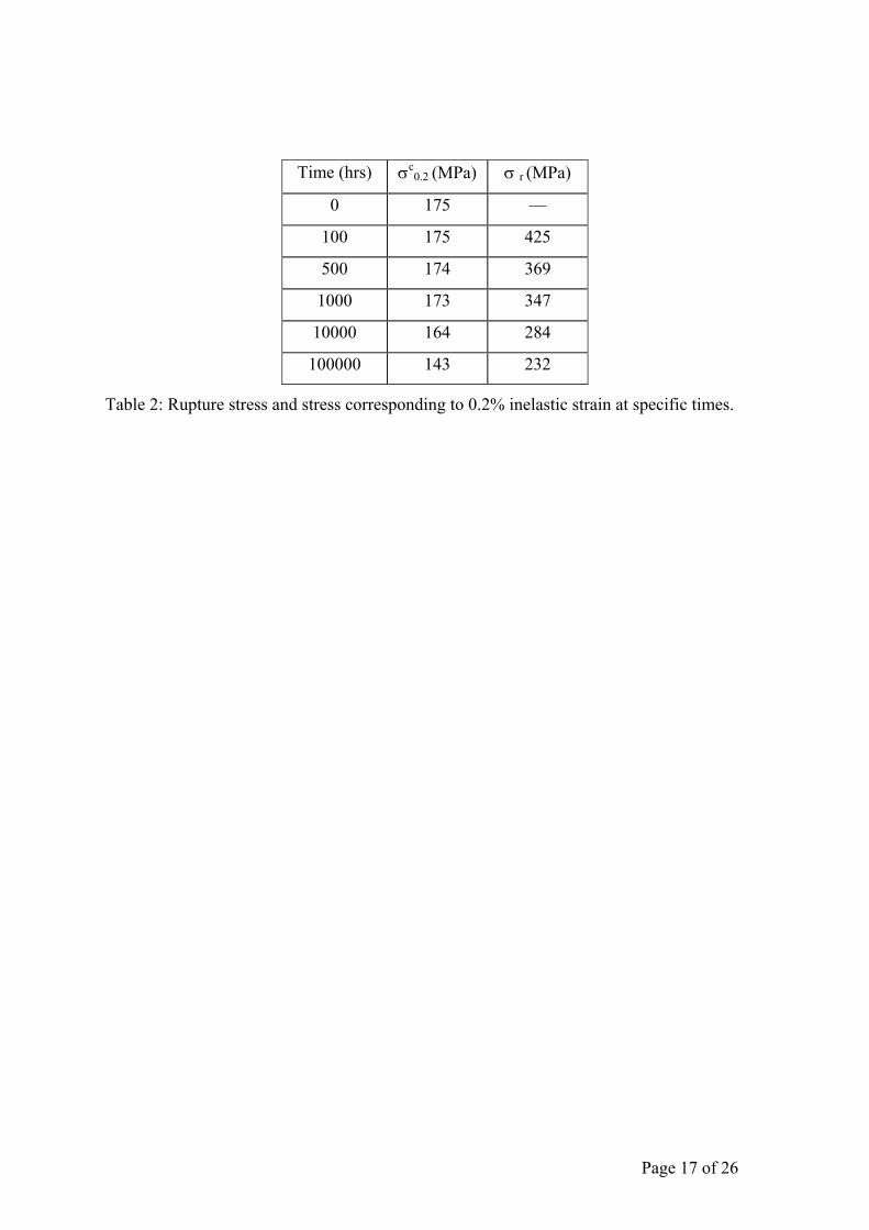
Isochronous stress strain curves based on Eqs. (13) to (15) have been produced for the times

listed in Table 2, examples of which are shown in Figure 6. It may be seen that the

isochronous stress strain curves are relatively independent of time for times below 1000 hrs.

Values of the 0.2% stress, , taken from these curves together with values of rupture stress

are given in

c2.0σ

Table 2.

Regression analysis of rupture time vs. stress, from the uniaxial creep data in [4], provided

the values of the constants in the creep rupture equation, Eq. (4), as B = 9.57 × 1031 and

v = 1.41, with stress in MPa and time in hours. Thus Eq. (4) in conjunction with Eq. (3) can

be used to determine Lrmax at different times.

Page 9 of 26

4 Results

4.1 Creep Toughness

4.1.1 Variation of Creep Toughness with Time and Data Bounds of cmatK

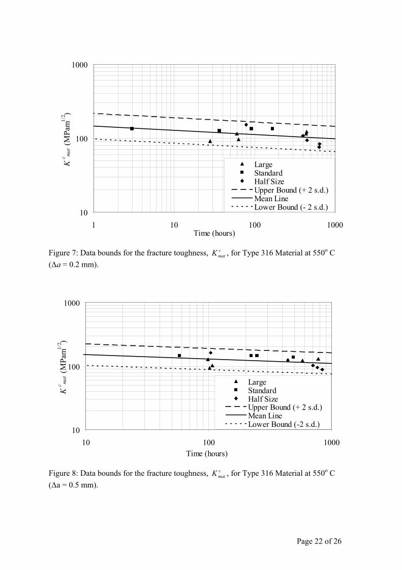
The creep toughness data from each test have been combined to determine the relationship

between and time at temperature, T = 550cmatK oC and crack extensions of Δa = 0.2 mm and

Δa = 0.5 mm as illustrated in Figure 7 and Figure 8, respectively. Different symbols have

been used in the figures to illustrate the data for the different specimen size, although no

obvious trend with specimen size is observed. A mean trend line was fitted to the data

as shown in

cmatK

Figure 7 and Figure 8.

If the creep toughness is assumed to follow a normal distribution, then upper and lower

bound values can be determined by offsetting the mean line in cmatK Figure 7 and Figure 8 to

the data by ± 2 standard deviations (s.d.). These data bounds are shown in Figure 7 and

Figure 8. By comparing Figure 7 and Figure 8 it may be seen that defining initiation at Δa =

0.2 mm will lead to a lower value of , with a somewhat higher associated scatter,

compared to that obtained using Δa = 0.5 mm. It is also apparent that the creep toughness is

high, and not significantly reduced by creep in the timescales of these tests.

cmatK

4.1.2 Sensitivity of Creep Toughness to the Area under the Loading Curve

Typical experimental load-displacement curves from the tests on CT specimens are illustrated

in Figure 9 up to Δa = 0.5mm, where the load, P, has been normalised by the width, W, and

thickness, B, of these (plane sided) specimens, and the Young’s modulus of the material, E.

The displacement here, which has been normalised into non-dimensional form by the

specimen width, W, is the total axial displacement that includes the elastic, plastic and creep

displacements. Note that the linear portion of the curve for the large and half size specimens

(L and HS in Figure 9, respectively) should lie very close to each other when plotted in this

normalised form, since the specimens are geometrically similar (a/W = 0.45, B/W ≈ 0.5 in

both cases). The measured stiffness during load-up of the large specimen is very close to the

theoretical value from [9], but the half size specimens exhibits a larger displacement. This is

likely to be due to experimental error and suggests that the elastic area in Figure 2 would be

better estimated from stress intensity factor solutions than from measured elastic

displacement, as in some J-estimation methods [9]. However, the measured variability in the

Page 10 of 26

loading curve for the HS specimen produces variability in creep toughness that is well within

the upper and lower bound toughness lines for in cmatK Figure 7.

It is seen in Figure 9 that for all the specimens, particularly the large CT specimen, a

significant proportion of the area under the loading curve corresponds to the elastic and

plastic area, i.e. creep initiation at these times is dominated by the elastic plastic response.

The evaluation of the area under the load up part of the curve can therefore be of significance

when calculating at short incubation times. This trend is illustrated more clearly in cmatK

Figure 10 where the ratio of the area under the loading part of the curve to the total area

under the curve, UL /UT is shown for the three specimen sizes. In the case of the large

specimen, the area under the load up part of the curve is about 90% of the total area under the

load displacement curve at the defined initiation increments (Δa = 0.2, 0.5 mm).

4.2 TDFAD for 316 H at 550oC

Time dependent failure assessment diagrams, for the times listed in Table 2, have been

produced for this material at 550oC. The R6 Option 1 FAD [1], which is applicable at low

temperatures has also been determined. These diagrams are shown in Figure 11 and Figure

12, respectively. At times of 100 hrs and below, the value of given by Eq. maxrL (3), exceeds

that obtained from an R6 analysis. would therefore be set equal to the value given by the

R6 procedure as discussed in Section

maxrL

2.

The TDFAD at time zero is compared to the R6 Option 1 curve in Figure 11. Both curves lie

close to each other especially at lower values of Lr. Figure 12 shows the evolution of the

TDFAD up to a time of 100,000 hours. It is observed that the TDFAD is quite insensitive to

time and the greatest noticeable difference between the diagrams at each time is the cut off

value, , which decreases as time increases, indicating the reduction of time to failure by

continuum damage, due to the reduction in σ

maxrL

r with increasing time via Eq. (4). The

insensitivity of the curves in Figure 12 to time is due to the high value of creep stress

exponent, n, in the creep strain equation (see Eq. (13)) which may not be valid at the longer

times.

5 Application of TDFAD to Predict Initiation Times

An example of the use of a TDFAD to predict initiation times is presented as an illustration

of the application of the method. The initiation time of a test on a standard sized CT

Page 11 of 26

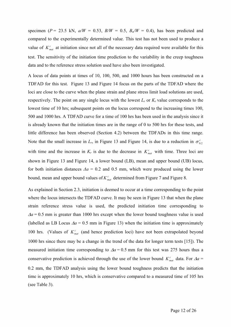
specimen (P = 23.5 kN, a/W = 0.53, B/W = 0.5, BBn/W = 0.4), has been predicted and

compared to the experimentally determined value. This test has not been used to produce a

value of at initiation since not all of the necessary data required were available for this

test. The sensitivity of the initiation time prediction to the variability in the creep toughness

data and to the reference stress solution used have also been investigated.

cmatK

A locus of data points at times of 10, 100, 500, and 1000 hours has been constructed on a

TDFAD for this test. Figure 13 and Figure 14 focus on the parts of the TDFAD where the

loci are close to the curve when the plane strain and plane stress limit load solutions are used,

respectively. The point on any single locus with the lowest Lr or Kr value corresponds to the

lowest time of 10 hrs; subsequent points on the locus correspond to the increasing times 100,

500 and 1000 hrs. A TDFAD curve for a time of 100 hrs has been used in the analysis since it

is already known that the initiation times are in the range of 0 to 500 hrs for these tests, and

little difference has been observed (Section 4.2) between the TDFADs in this time range.

Note that the small increase in Lr, in Figure 13 and Figure 14, is due to a reduction in

with time and the increase in K

c2.0σ

r is due to the decrease in with time. Three loci are

shown in

cmatK

Figure 13 and Figure 14, a lower bound (LB), mean and upper bound (UB) locus,

for both initiation distances Δa = 0.2 and 0.5 mm, which were produced using the lower

bound, mean and upper bound values of determined from cmatK Figure 7 and Figure 8.

As explained in Section 2.3, initiation is deemed to occur at a time corresponding to the point

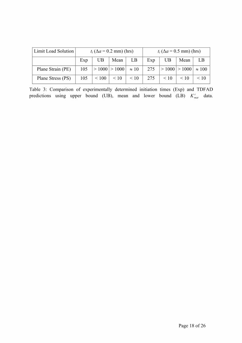
where the locus intersects the TDFAD curve. It may be seen in Figure 13 that when the plane

strain reference stress value is used, the predicted initiation time corresponding to

Δa = 0.5 mm is greater than 1000 hrs except when the lower bound toughness value is used

(labelled as LB Locus Δa = 0.5 mm in Figure 13) when the initiation time is approximately

100 hrs. (Values of (and hence prediction loci) have not been extrapolated beyond

1000 hrs since there may be a change in the trend of the data for longer term tests [15]). The

measured initiation time corresponding to Δa = 0.5 mm for this test was 275 hours thus a

conservative prediction is achieved through the use of the lower bound data. For Δa =

0.2 mm, the TDFAD analysis using the lower bound toughness predicts that the initiation

time is approximately 10 hrs, which is conservative compared to a measured time of 105 hrs

(see

cmatK

cmatK

Table 3).

Page 12 of 26

If the plane stress reference stress definition is used, as illustrated in Figure 14, it may be

seen that the initiation time for the specimen (for Δa = 0.2 or 0.5 mm) is less than 100 hrs

regardless of whether the lower, mean or upper bound value is used for the creep toughness,

. This illustrates the strong dependence of the result on the choice of reference stress

solution.

cmatK

The initiation times predicted by this method using the loci corresponding to mean, upper

bound (UB) and lower bound (LB) values of and the plane stress and plane strain von

Mises limit load solutions are compared to the experimentally determined initiation times in

cmatK

Table 3. Although this side-grooved, standard-sized test specimen may be expected to be

represented more closely by the plane strain solution than plane stress, the initiation times

predicted by a plane strain analysis are not conservative, unless the lower bound creep

toughness is used.

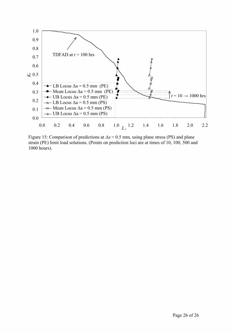
A direct comparison is made in Figure 15 of the results obtained using the plane strain or the

more conservative plane stress von Mises reference stress solution for Δa = 0.5 mm. On this

scale the prediction loci are close to being vertical since, as can be seen in Table 2, is

approximately constant over the timescale considered, and the only significant change is in

. The shift in the data due to the use of the different reference stress solutions is clearly

observed. For this specimen the plane stress solution gives an L

c2.0σ

cmatK

r value 1.44 times greater than

that from the plane strain solution (see Eq. (11)) and the effects on the predicted initiation

times are significant.

The sensitivity to the reference stress solution will depend on the region of the TDFAD in

which the prediction loci are situated. For this material and temperature the failure

assessment curve is approximately horizontal for values of Lr greater than 1.7. Thus, a

horizontal shift to the locus, due to the use of a different reference stress solution, will have

very little effect on initiation time predictions in the region Lr > 1.7. Similarly if the loci fall

in the region, Lr < 0.5, the results will not be very sensitive to the choice of reference stress

solution. However, as illustrated above, if the loci fall in the region, 0.5 < Lr < 1.4 the

predicted initiation times can decrease by up to two orders of magnitude when the reference

stress increases by less than 50 percent.

Page 13 of 26

6 Conclusions

Creep toughness values, , have been determined for austenitic Type 316H stainless steel

at 550

cmatK

oC from analysis of fourteen creep crack growth tests on CT specimens of different

sizes and thickness. Values of were obtained for two initiation distances, Δa = 0.2 mm

and Δa = 0.5 mm. It has been found that for the 316 steel at 550

cmatK

oC the area under the loading

part of the curve in a creep crack growth (CCG) test, which is used to determine , cannot

be neglected. Accurate data from the load-up part of a CCG test are therefore essential in

determining accurate values of . Time dependent failure assessment diagrams (TDFAD)

have been produced at various assessment times and the shape of the curve is found to be

insensitive to time. Initiation times have been predicted using the TDFAD approach and the

lower bound, mean and upper bound values, with both the plane stress and plane strain

reference stress solution used in the calculation of L

cmatK

cmatK

cmatK

r. When the plane strain reference stress

solution is used conservative predictions have been obtained only through the use of the

lower bound values. However, the plane stress solution has resulted in conservative

predictions when used with all bounds of .

cmatK

cmatK

Acknowledgements

The assistance of Mr. Kilian Wasmer in the statistical analysis of the data is gratefully

acknowledged. This paper is published with permission of British Energy Generation.

References

1. British Energy Generation Ltd., “R6: Assessment of the Integrity of Structures Containing Defects”, Revision 4, British Energy Generation Ltd., 2001.

2. Ainsworth R.A., Hooton, D. G. and Green, D., “Failure Assessment Diagrams for High Temperature Defect Assessment”, Engineering Fracture Mechanics, 62, pp. 95-109, 1999.

3. Webster G.A., Ainsworth, R. A., “High Temperature Component Life Assessment”, 1st ed., Chapman and Hall, London, 1994.

4. Bettinson A.D., “The Influence of Constraint on the Creep Crack Growth of 316H Stainless Steel”, Ph.D. Thesis, Department of Mechanical Engineering, Imperial College London, 2002.

5. ASME, “Case of ASME Boiler and Pressure Vessel Code”, Section III-Class I Components in Elevated Temperature Service. Code Case N47-29, New York, 1990.

6. RCC-MR, “Design and Construction Rules for Mechanical Components of FBR Nuclear Island”, AFCEN, 1985.

Page 14 of 26

7. Dean D.W., O’Donnell, M. P. “Alternative Approaches in the R5 Procedures for Predicting Initiation and the Early Stages of Creep Crack Growth”, Creep and Fatigue at Elevated Temperatures, Tsukuba, Japan, 2001, pp. 315-319.

8. ESIS, “ESIS Procedure for Determining the Fracture Behaviour of Materials”, ESIS P2-92, European Structural Integrity Society, 1992.

9. ASTM, “ASTM E 1820-01: Standard Test Method for Measurement of Fracture Toughness”, Annual Book of ASTM Standards, 2001.

10. Dean D.W., Ainsworth, R.A., Booth, S.E., “Development and Use of the R5 Procedures for the Assessment of Defects in High Temperature Plant”, International Journal of Pressure Vessels and Piping, 78, pp. 963-976, 2001.

11. Bettinson A.D., O’Dowd, N.P., Nikbin K.M., Webster G.A., “Experimental investigation of constraint effects on creep crack growth”, PVP, 434, Computational Weld Mechanics, Constraint and Weld Fracture, ASME 2002, Ed. F.W. Brust, ASME New York, NY 10016 2002, pp. 143-150.

12. Djavanroodi F., Webster G.A., “Comparison Between Numerical and Experimental Estimates of the Creep Fracture Parameter C*”, Fracture Mechanics, Philadelphia, 1992, pp. 271-283.

13. Miller A.G., “Review of Limit Loads of Structures Containing Defects”, International Journal of Pressure Vessel and Piping, 32, pp. 197-327, 1988.

14. RCC-MR, “Design and Construction Rules for Mechanical Components of FBR Nuclear Islands”, AFCEN, 1995.

15. Dean D.W., Gladwin, D.N. “Characterisation of Creep Crack Growth Behaviour in Type 316H Steel Using Both C* and Creep Toughness Parameters”, Proc 9th Int. Conf. on Creep and Fracture of Engineering Materials and Structures, Swansea, 2001, pp. 751-761.

Page 15 of 26

Specimen Size Width W (mm)

Thickness B (mm)

Net Thickness BBn (mm)

Large (L) 104 50 50 Standard (S) 50 25 25

Half size (HS) 26 13 13

Table 1: Typical dimensions of compact tension specimens used in the analysis.

Page 16 of 26

Time (hrs) σc0.2 (MPa) σ r (MPa)

0 175 —

100 175 425

500 174 369

1000 173 347

10000 164 284

100000 143 232

Table 2: Rupture stress and stress corresponding to 0.2% inelastic strain at specific times.

Page 17 of 26

Limit Load Solution ti (Δa = 0.2 mm) (hrs) ti (Δa = 0.5 mm) (hrs)

Exp UB Mean LB Exp UB Mean LB

Plane Strain (PE) 105 > 1000 > 1000 ≈ 10 275 > 1000 > 1000 ≈ 100

Plane Stress (PS) 105 < 100 < 10 < 10 275 < 10 < 10 < 10

Table 3: Comparison of experimentally determined initiation times (Exp) and TDFAD predictions using upper bound (UB), mean and lower bound (LB) data.c

matK

Page 18 of 26

0.002 Total Strain

Figure 1: Schematic isochronous stress strain curve, after [10] indicating the definition of and c

2.0σ refσ .

Figure 2: Schematic load-displacement behaviour in a creep crack growth test, after [10].

Total Displacement

Load

Up Uc Ue

Δp Δc Δe

Stress – Strain Curve (t = 0)

Isochronous Stress – Strain Curve

Stress

c2.0σ

σref

σ0.2

(t > 0)

ε ref

Page 19 of 26

t = 0 t = 3000 h t = 300,000 h

R6 Option 1 1.0

0

0.8

0.6

0.4

0.2

0.2 0.4 0.6 0.8 1.0 1.2 1.4

Kr

Lr

Figure 3: Schematic example of a time dependent failure assessment diagram (TDFAD) based on data from an austenitic steel [2].

0.0

0.1

0.2

0.3

0.4

0.5

0.6

0.7

0.8

0 40 80Time (hrs)

Crac

k Ex

tens

ion,

Δa

(mm

)

t i

Figure 4: Determination of initiation time, ti, for Δa = 0.5 mm from experimental data [4].

Page 20 of 26

0123456789

10

0.0 0.1 0.2 0.3 0.4 0.5

Δ (mm)

P (k

N)

P = 1367Δ 5 - 1535Δ 4 + 547Δ 3 - 77Δ 2 + 27Δ

Figure 5: Load, P, vs. displacement, Δ , data during load up in a test on a HS specimen.

0

50

100

150

200

250

300

0 1 2 3 4 5 6 7

Total Strain (%)

Stre

ss (M

Pa)

Tensile DataIsochronous Curve t = 100 hrsIsochronous Curve t = 1000 hrsIsochronous Curve t = 10000 hrsIsochronous Curve t = 100000 hrs

Figure 6: Isochronous stress-strain curves generated for 316H stainless steel at 550oC

Page 21 of 26

10

100

1000

1 10 100 1000Time (hours)

K c m

at (M

Pam1/

2 )

LargeStandardHalf SizeUpper Bound (+ 2 s.d.)Mean LineLower Bound (- 2 s.d.)

Figure 7: Data bounds for the fracture toughness, , for Type 316 Material at 550cmatK o C

(Δa = 0.2 mm).

10

100

1000

10 100 1000Time (hours)

K c m

at (M

Pam1/

2 )

LargeStandardHalf SizeUpper Bound (+ 2 s.d.)Mean LineLower Bound (-2 s.d.)

Figure 8: Data bounds for the fracture toughness, , for Type 316 Material at 550cmatK o C

(Δa = 0.5 mm).

Page 22 of 26

0.0E+00

5.0E-05

1.0E-04

1.5E-04

2.0E-04

0 0.01 0.02 0.03 0.04 0.05Δ T / W

P/(E

BW)

2.5E-04

LSHS

Figure 9: Typical normalised load-displacement curve for Large (L), Standard (S) and Half Size (HS) CT specimens in a CCG tests (up to Δa = 0.5 mm).

0.0

0.2

0.4

0.6

0.8

1.0

0.0 0.1 0.2 0.3 0.4 0.5Crack Extension, Δ a (mm)

UL /

UT

LSHS

Figure 10: Comparison of the ratio of the loading area, UL, to total area under, UT, the load displacement curve, as crack extension proceeds, for a Large (L), Standard (S) and Half Size (HS) CT specimen.

Page 23 of 26

0.0

0.1

0.2

0.3

0.4

0.5

0.6

0.7

0.8

0.9

1.0

0.0 0.2 0.4 0.6 0.8 1.0 1.2 1.4 1.6 1.8 2.0 2.2L r

Kr

R6 Option 1 FAD

TDFAD t = 0 hrs

Figure 11: TDFAD at time t = 0 hours and R6 Option 1 FAD.

0.0

0.1

0.2

0.3

0.4

0.5

0.6

0.7

0.8

0.9

1.0

0.0 0.2 0.4 0.6 0.8 1.0 1.2 1.4 1.6 1.8 2.0 2.2L r

Kr

TDFAD t = 0 hrsTDFAD t = 500 hrsTDFAD t = 1000 hrsTDFAD t = 10000 hrsTDFAD t = 100000 hrs

t = 0 hrs

t = 100000 hrs

Figure 12: TDFAD for austenitic Type 316H stainless steel over a range of times.

Page 24 of 26

0.0

0.1

0.2

0.3

0.4

0.5

0.6

0.7

0.8

0.9

1.0

1.00 1.02 1.04 1.06 1.08 1.10L r

KrLB Locus Δa = 0.2 mm LB Locus Δa = 0.5 mm Mean Locus Δa = 0.2 mm Mean Locus Δa = 0.5 mm UB Locus Δa = 0.2 mm UB Locus Δa = 0.5 mm

t = 0 → 1000 hrs

TDFAD at t = 100 hrs

Figure 13: Application of a TDFAD to predict initiation times of a test using the plane strain limit load solution.

Figure 14: Application of a TDFAD to predict initiation times of a test using the plane stress limit load solution.

0.0

0.1

0.2

0.3

0.4

0.5

0.6

0.7

0.8

0.9

1.0

1.40 1.42 1.44 1.46 1.48 1.50 1.52 1.54 1.56 1.58 1.60L r

Kr

LB Locus Δa = 0.2 mm LB Locus Δa = 0.5 mm Mean Locus Δa = 0.2 mm Mean Locus Δa = 0.5 mm UB Locus Δa = 0.2 mm UB Locus a = 0.5 mm

t = 10 → 1000 hrs

TDFAD at t = 100 hrs

Δ

Page 25 of 26

0.0

0.1

0.2

0.3

0.4

0.5

0.6

0.7

0.8

0.9

1.0

0.0 0.2 0.4 0.6 0.8 1.0 1.2 1.4 1.6 1.8 2.0 2.2L r

Kr

LB Locus Δa = 0.5 mm (PE) Mean Locus Δa = 0.5 mm (PE) UB Locus Δa = 0.5 mm (PE) LB Locus Δa = 0.5 mm (PS) Mean Locus Δa = 0.5 mm (PS) UB Locus Δa = 0.5 mm (PS)

TDFAD at t = 100 hrs

t = 10 → 1000 hrs

Figure 15: Comparison of predictions at Δa = 0.5 mm, using plane stress (PS) and plane strain (PE) limit load solutions. (Points on prediction loci are at times of 10, 100, 500 and 1000 hours).

Page 26 of 26