Faculty of Health and Applied Sciences

NAMIBIA UNIVERSITY OF SCIENCE AND TECHNOLOGY

Faculty of Health and Applied Sciences

Department of Mathematics and Statistics

QUALIFICATIONS: B. Business Admin, B. Marketing, B. Human Resource Management, B. Public Management and B. Logistics and Supply Chain Management

QUALIFICATION CODES: 21BBAD / 07BMAR / LEVEL: 6 O7BHR / 24BPN / 07BLSM ,

COURSE: BASIC BUSINESS STATISTICS 1B COURSE CODE: BBS112S

DATE: JANUARY 2020 SESSION: 1

DURATION: 3 HOURS MARKS: 100

SECOND OPPORTUNITY/SUPPLEMENTARY EXAMINATION QUESTION PAPER

EXAMINER(S) MR EM MWAHI, MS A SAKARIA, MR | NDADI, MR G MBOKOMA, MRR MUMBUU,

MR A ROUX, MR G TAPEDZESA

MODERATOR: MR JJ SWARTZ

THIS QUESTION PAPER CONSISTS OF 7 PAGES

(Including this front page)

INSTRUCTIONS

1. Answer all the questions and number your solutions correctly. 2. Question 1 of this question paper entails multiple choice questions with options A to

D. Write down the letter corresponding to the best option for each question. 3. For Question 2, 3 & 4 you are required to show clearly all the steps used in the

calculations.

4. All written work MUST be done in blue or black ink. 5. Untidy/ illegible work will attract no marks.

PERMISSIBLE MATERIALS

1. Non-Programmable Calculator without the cover

ATTACHMENTS

1. Standard normal Z-table, Student t-table and Chi-square table.

QUESTION 1 [30 MARKS]

1.1 If true value of population parameter is 10 and estimated value of population

parameter is 15 then error of estimation is: [2]

A.5 B. 25

c.1.5 D. 0.667

1.2 Parameters and statistics... [2]

A. Are both used to make inferences about the sample mean.

B. Describe the population and the sample, respectively.

C. Describe the sample and the population, respectively.

D. Describe the same group of individuals.

1.3 What should be the critical value of z used in a 93% confidence interval? [2] *

A. 2.70 B. 1.40

Cc. 1.81 D. 1.89

1.4 Arandom sample of 100 observations is to be drawn from a population with a mean

of 40 and a standard deviation of 25. The probability that the mean of the sample

will exceed 45 is? [2]

A. 0.477 B. 0.4207

C. 0.0793 D. 0.0228

1.5 Suppose we sample by selecting every fifth invoice in a file after randomly obtaining

a starting point. What type of sampling is this? [2]

A. Simple random sampling. B. Cluster random sampling.

C. Stratifies random sampling. D. Systematic random sampling.

1.6

1.7

1.8

1.9

1.10

A 95% confidence interval for a population mean is determined to be 100 to 120. If

the confidence level is reduced to 90%, the interval: [2]

A. Becomes narrower. B. Becomes wider.

C. Does not change. D. Becomes 0.1.

An interval estimate is a range of values used to estimate: [2]

A. The shape of the population's distribution.

B. The sampling distribution.

C. Asample statistic.

D. A population parameter.

Suppose that we wanted to estimate the true average number of eggs a queen bee

lays with 95% confidence. The margin of error we are willing to accept is 0.5.

Suppose we also know that the population standard deviation is 10. What sample

size should we use? [2]

A. 1536 B. 1537

C. 2653 D. 2650

The null and alternative hypotheses divide all possibilities into: [2]

A. two sets that overlap

B. two non-overlapping sets

C. two sets that may or may not overlap

D. as many sets as necessary to cover all possibilities

The form of the alternative hypothesis can be: [2]

A. one-tailed B. two-tailed

C. neither one nor two-tailed D. one or two-tailed

1.11

1.12

1.13

1.14

1.15

Which of the following is true of the null and alternative hypotheses? [2]

A. Exactly one hypothesis must be true

B. both hypotheses must be true

C. It is possible for both hypotheses to be true

D. It is possible for neither hypothesis to be true

A type Il error occurs when: [2]

A. the null hypothesis is incorrectly accepted when it is false

B. the null hypothesis is incorrectly rejected when it is true

C. the sample mean differs from the population mean

D. the test is biased

Test of hypothesis Ho: 1 = 50 against H1: p > 50 leads to: [2]

A. Left-tailed test B. Right-tailed test

C. Two-tailed test D. Difficult to tell

When ois known, the hypothesis about population mean is tested by: [2]

A. t-test B. Z-test

C. x2-test D. F-test

The purpose of statistical inference is: [2]

A. To collect sample data and use them to formulate hypotheses about a population

B. To draw conclusion about populations and then collect sample data to support the

conclusions

C. To draw conclusions about populations from sample data

D. To draw conclusions about the known value of population parameter

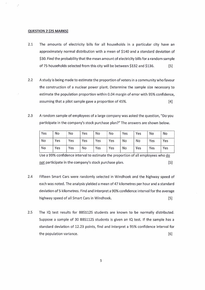
QUESTION 2 [25 MARKS]

Zak

2.2

2.3

2.4

2.5

The amounts of electricity bills for all households in a particular city have an

approximately normal distribution with a mean of $140 and a standard deviation of

$30. Find the probability that the mean amount of electricity bills for a random sample

of 75 households selected from this city will be between $132 and $136. [5]

A study is being made to estimate the proportion of voters in a community who favour

the construction of a nuclear power plant. Determine the sample size necessary to

estimate the population proportion within 0.04 margin of error with 95% confidence,

assuming that a pilot sample gave a proportion of 45%. [4]

A random sample of employees of a large company was asked the question, "Do you

participate in the company's stock purchase plan?" The answers are shown below.

Yes No No Yes No No Yes Yes No No

No Yes Yes Yes Yes Yes No No Yes Yes

No Yes Yes No Yes Yes No Yes Yes Yes

Use a 99% confidence interval to estimate the proportion of all employees who do

not participate in the company's stock purchase plan. [5]

Fifteen Smart Cars were randomly selected in Windhoek and the highway speed of

each was noted. The analysis yielded a mean of 47 kilometres per hour and a standard

deviation of 5 kilometres. Find and interpret a 90% confidence interval for the average

highway speed of all Smart Cars in Windhoek. [5]

The IQ test results for BBS112S students are known to be normally distributed.

Suppose a sample of 30 BBS112S students is given an IQ test. If the sample has a

standard deviation of 12.23 points, find and interpret a 95% confidence interval for

the population variance. [6]

QUESTION 3 [19 MARKS]

3.1

3.2

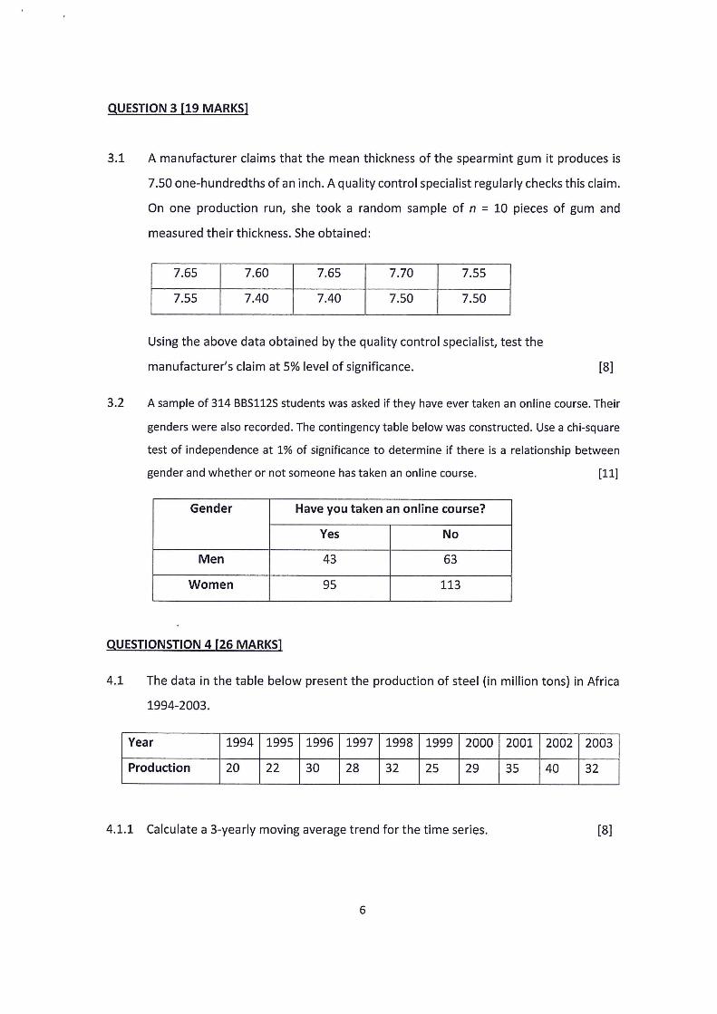
A manufacturer claims that the mean thickness of the spearmint gum it produces is

7.50 one-hundredths of aninch. A quality control specialist regularly checks this claim.

On one production run, she took a random sample of n = 10 pieces of gum and

measured their thickness. She obtained:

7.65 7.60 7.65 7.70 7.55

7.55 7.40 7.40 7.50 7.50

Using the above data obtained by the quality control specialist, test the

manufacturer’s claim at 5% level of significance. [8]

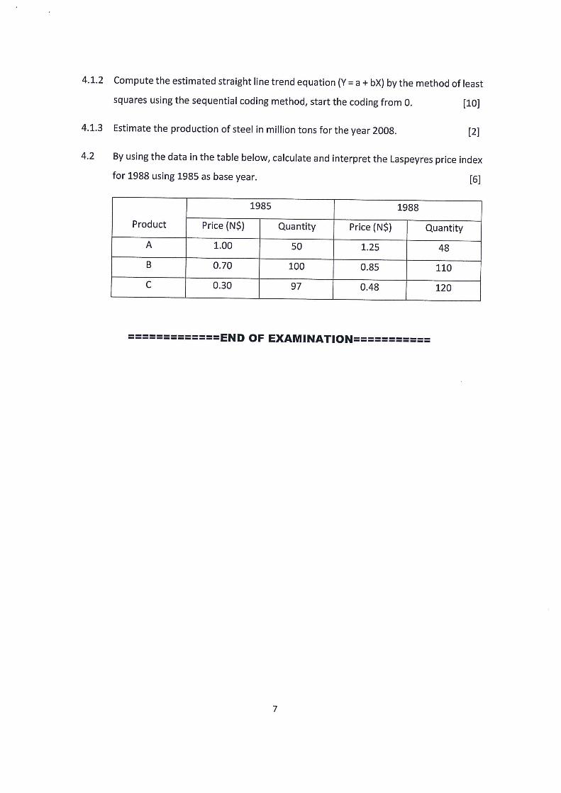
A sample of 314 BBS112S students was asked if they have ever taken an online course. Their

genders were also recorded. The contingency table below was constructed. Use a chi-square

test of independence at 1% of significance to determine if there is a relationship between

gender and whether or not someone has taken an online course. [11]

Gender Have you taken an online course?

Yes No

Men 43 63

Women 95 113

QUESTIONSTION 4 [26 MARKS]

4.1 The data in the table below present the production of steel (in million tons) in Africa

1994-2003.

Year 1994 | 1995 | 1996 | 1997 | 1998 | 1999 | 2000 | 2001 | 2002 | 2003

Production 20 22 30 28 32 25 29 35 40 32

4.1.1 Calculate a 3-yearly moving average trend for the time series. [8]

4.1.2

4.1.3

4.2

Compute the estimated straight line trend equation (Y = a + bX) by the method of least

squares using the sequential coding method, start the coding from 0. [10]

Estimate the production of steel in million tons for the year 2008. [2]

By using the data in the table below, calculate and interpret the Laspeyres price index

for 1988 using 1985 as base year. [6]

1985 1988

Product Price (NS) Quantity Price (NS) Quantity

A 1.00 50 1.25 48

B 0.70 100 0.85 110

C 0.30 97 0.48 120

S=S==========END OF EXAMINATION========2=2=

5217X_IBC.indd 1

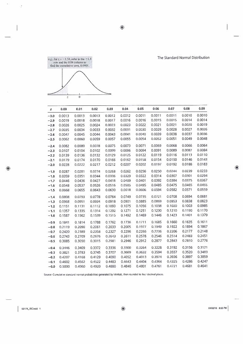
e.g., for z= —1.34, refer to the — 13 row and the 0.04 column to

find the cumulative area, 0.0901. a

The Standard Normal Distribution

z 0.00 0.01 0.02 0.03 0.04 0.05 0.06 0.07 0.08 0.09

-3.0 0.0013 0.0013 0.0013 0.0012 0.0012 0.0011 0.0011 0.0011 0.0010 0.0010

-2.9 0.0019 0.0018 0.0018 0.0017 0.0016 0.0016 0.0015 0.0015 0.0014 0.0014

-2.8 0.0026 0.0025 0.0024 0.0023 0.0023 0.0022 0.0021 0.0021 0.0020 0.0019

-2.7. 0.0035 0.0034 0.0033 0.0032 0.0031 0.0030 0.0029 0.0028 0.0027 0.0026

-2.6 0.0047 0.0045 0.0044 0.0043 0.0041 0.0040 0.0039 0.0038 0.0037 0.0036

-2.5 0.0062 0.0060 0.0059 0.0057 0.0055 0.0054 0.0052 0.0051 0.0049 0.0048

-2.4 0.0082 0.0080 0.0078 0.0075 0.0073 0.0071 0.0069 0.0068 0.0066 0.0064

-2.3 0.0107 0.0104 0.0102 0.0099 0.0096 0.0094 0.0091 0.0089 0.0087 0.0084

-2.2 0.0139 0.0136 0.0132 0.0129 0.0125 0.0122 0.0119 0.0116 0.0113 0.0110

-2.1 0.0179 0.0174 0.0170 0.0166 0.0162 0.0158 0.0154 0.0150 0.0146 0.0143

—2.0 0.0228 0.0222 0.0217 0.0212 0.0207 0.0202 0.0197 0.0192 0.0188 0.0183

-1.9 0.0287 0.0281 0.0274 0.0268 0.0262 0.0256 0.0250 0.0244 0.0239 0.0233

-1.8 0.0359 0.0351 0.0344 0.0336 0.0329 0.0322 0.0314 0.0307 0.0301 0.0294

-1.7 0.0446 0.0436 0.0427 0.0418 0.0409 0.0401 0.0392 0.0384 0.0375 0.0367

-16 0.0548 0.0537 0.0526 0.0516 0.0505 0.0495 0.0485 0.0475 0.0465 0.0455

-1.5 0.0668 0.0655 0.0643 0.0630 0.0618 0.0606 0.0594 0.0582 0.0571 0.0559

-1.4 0.0808 0.0793 0.0778 0.0764 0.0749 0.0735 0.0721 0.0708 0.0694 0.0681

-1.3 0.0968 0.0951 0.0934 0.0918 0.0901 0.0885 0.0869 0.0853 0.0838 0.0823

—1.2 0.1151 0.1131 0.1112 0.1093 0.1075 0.1056 0.1038 0.1020 0.1003 0.0985

-1.1 0.1357 0.1335 0.1314 0.1292 0.1271 0.1251 0.1230 0.1210 0.1190 0.1170

-1.0 0.1587 0.1562 0.1539 0.1515 0.1492 0.1469 0.1446 0.1423 0.1401 0.1379

-0.9 0.1841 0.1814 0.1788 0.1762 0.1736 0.1711 0.1685 0.1660 0.1635 0.1611

-0.8 0.2119 0.2090 0.2061 0.2033 0.2005 0.1977 0.1949 0.1922 0.1894 0.1867

-0.7. 0.2420 0.2389 0.2358 0.2327 0.2296 0.2266 0.2236 0.2206 0.2177 0.2148

-0.6 0.2743 0.2709 0.2676 0.2643 0.2611 0.2578 0.2546 0.2514 0.2483 0.2451

-0.5 0.3085 0.3050 0.3015 0.2981 0.2946 0.2912 0.2877 0.2843 0.2810 0.2776

-0.4 0.3446 0.3409 0.3372 0.3336 0.3300 0.3264 0.3228 0.3192 0.3156 0.3121

-0.3 0.3821 0.3783 0.3745 0.3707 0.3669 0.3632 0.3594 0.3557 0.3520 0.3483

-0.2 0.4207 0.4168 0.4129 0.4090 0.4052 0.4013 0.3974 0.3936 0.3897 0.3859

-0.1 0.4602 0.4562 0.4522 0.4483 0.4443 0.4404 0.4364 0.4325 0.4286 0.4247

-0.0 0.5000 0.4960 0.4920 0.4880 0.4840 0.4801 0.4761 0.4721 0.4681 0.4641

Source: Cumulative standard normal probabilities generated by Minitab, then rounded to four decimal places.

04/02/10 8:53 PM

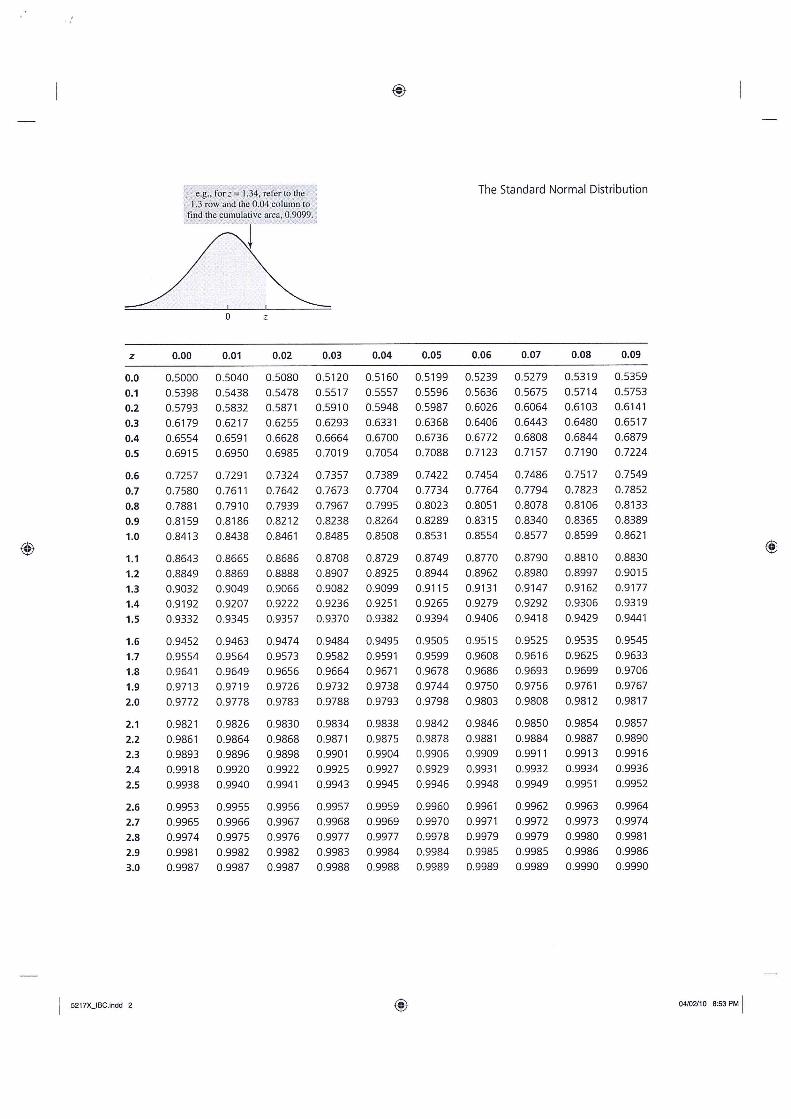
e.g., for z = 1.34, refer to the 1,3 row and the 0.04 column to

find the cumulative area, 0.9099.

!

The Standard Normal Distribution

z 0.00 0.01 0.02 0.03 0.04 0.05 0.06 0.07 0.08 0.09

0.0 0.5000 0.5040 0.5080 0.5120 0.5160 0.5199 0.5239 0.5279 0.5319 0.5359

0.1 0.5398 0.5438 0.5478 0.5517 0.5557 0.5596 0.5636 0.5675 0.5714 0.5753

0.2 0.5793 0.5832 0.5871 0.5910 0.5948 0.5987 0.6026 0.6064 0.6103 0.6141

0.3 0.6179 0.6217 0.6255 0.6293 0.6331 0.6368 0.6406 0.6443 0.6480 0.6517

0.4 0.6554 0.6591 0.6628 0.6664 0.6700 0.6736 0.6772 0.6808 0.6844 0.6879

0.5 0.6915 0.6950 0.6985 0.7019 0.7054 0.7088 0.7123 0.7157 0.7190 0.7224

0.6 0.7257 0.7291 0.7324 0.7357 0.7389 0.7422 0.7454 0.7486 0.7517 0.7549

0.7 0.7580 0.7611 0.7642 0.7673 0.7704 0.7734 0.7764 0.7794 0.7823 0.7852

0.8 0.7881 0.7910 0.7939 0.7967 0.7995 0.8023 0.8051 0.8078 0.8106 0.8133

0.9 0.8159 0.8186 0.8212 0.8238 0.8264 0.8289 0.8315 0.8340 0.8365 0.8389

1.0 0.8413 0.8438 0.8461 0.8485 0.8508 0.8531 0.8554 0.8577 0.8599 0.8621

1.1 0.8643 0.8665 0.8686 0.8708 0.8729 0.8749 0.8770 0.8790 0.8810 0.8830

1.2 0.8849 0.8869 0.8888 0.8907 0.8925 0.8944 0.8962 0.8980 0.8997 0.9015

1.3 0.9032 0.9049 0.9066 0.9082 0.9099 0.9115 0.9131 0.9147 0.9162 0.9177

1.4 0.9192 0.9207 0.9222 0.9236 0.9251 0.9265 0.9279 0.9292 0.9306 0.9319

1.5 0.9332 0.9345 0.9357 0.9370 0.9382 0.9394 0.9406 0.9418 0.9429 0.9441

1.6 0.9452 0.9463 0.9474 0.9484 0.9495 0.9505 0.9515 0.9525 0.9535 0.9545

1.7 0.9554 0.9564 0.9573 0.9582 0.9591 0.9599 0.9608 0.9616 0.9625 0.9633

1.8 0.9641 0.9649 0.9656 0.9664 0.9671 0.9678 0.9686 0.9693 0.9699 0.9706

1.9 0.9713 0.9719 0.9726 0.9732 0.9738 0.9744 0.9750 0.9756 0.9761 0.9767

2.0 0.9772 0.9778 0.9783 0.9788 0.9793 0.9798 0.9803 0.9808 0.9812 0.9817

2.1 0.9821 0.9826 0.9830 0.9834 0.9838 0.9842 0.9846 0.9850 0.9854 0.9857

2.2 0.9861 0.9864 0.9868 0.9871 0.9875 0.9878 0.9881 0.9884 0.9887 0.9890

2.3 0.9893 0.9896 0.9898 0.9901 0.9904 0.9906 0.9909 0.9911 0.9913 0.9916

2.4 0.9918 0.9920 0.9922 0.9925 0.9927 0.9929 0.9931 0.9932 0.9934 0.9936

2:5 0.9938 0.9940 0.9941 0.9943 0.9945 0.9946 0.9948 0.9949 0.9951 0.9952

2.6 0.9953 0.9955 0.9956 0.9957 0.9959 0.9960 0.9961 0.9962 0.9963 0.9964

2.7 0.9965 0.9966 0.9967 0.9968 0.9969 0.9970 0.9971 0.9972 0.9973 0.9974

2.8 0.9974 0.9975 0.9976 0.9977 0.9977 0.9978 0.9979 0.9979 0.9980 0.9981

2.9 0.9981 0.9982 0.9982 0.9983 0.9984 0.9984 0.9985 0.9985 0.9986 0.9986

3.0 0.9987 0.9987 0.9987 0.9988 0.9988 0.9989 0.9989 0.9989 0.9990 0.9990

5217X_IBC.indd 2 04/02/10 8:53PM

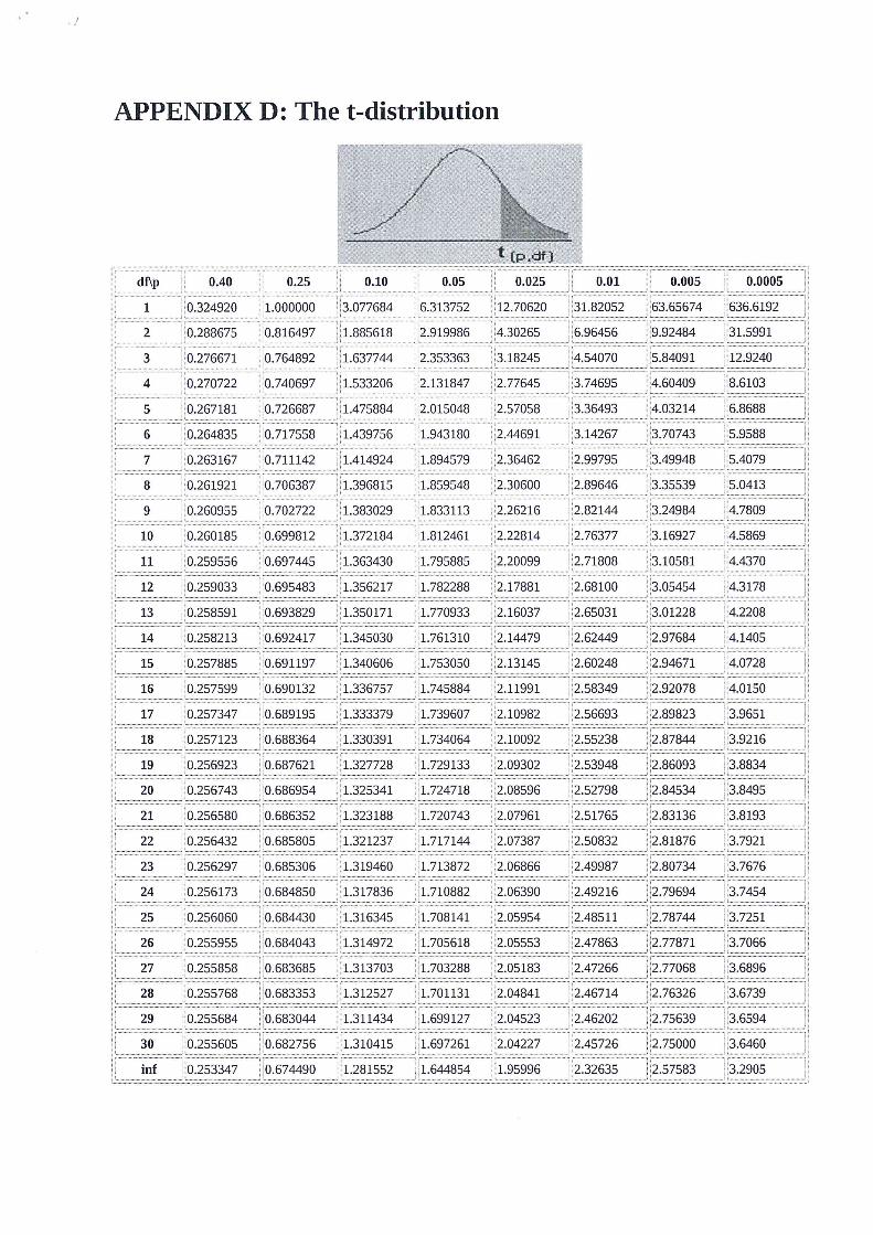
APPENDIX D: The t-distribution

0.816497 1.000000

om aa 0.005 0.0005

31.82052

636.6192

"31.5991 6.96456

764892

740697

533206

T5884

“4.54070

2.131847 3.74695

3.36493

12.9240

264835

0.263167 0.717558

0.711142,

414924

“1.943180

1.894579

3.14267

+ 2.99795

0.261921

0.260955 "0.702722

0.706387 _

396815)

1.859548

/ 1.383029

2.89646

2.82144

0.260185 0.699812 1.812461 2.76377

0.259556 "0.697445

“1.372184 "2.71808

0.259033 0.695483 1.782288

2.68100

0.258591

0.693829

1.770933 2.16037 2.65031

0.258213

0.692417

0.691197

1.340606

1.761310 "2.14479 2.62449 "1.753050

© 0.257347 0.257599 0.690132

0.689195

1.336757

2.60248

“1.745884 2.11991 2.58349

1.739607 2.10982 2.56693

0.257123

0.688364

1.330391

1.734064

"0.256923 0.687621 1.327728 1.729133 _

"2.55238

2.53948

0.256743 0.686954 /1.325341 2.52798

/ 0.256580 0.686352

1.724718

"2.51765

0.256432

0.685805

1.321237 |

0.256297

0.685306

Saeco nee

1.717144

2.50832

1.713872

2.49987

.256173

0.684850 (1.317836

0.256060 0.684430

1.710882 (2.49216

1.708141

0.255955 0.684043

0.255858 (0.683685

2.48511

“1.705618 (2.47863

1.703288

2.05183 2.47266 (0.255768 684

‘0.683353

1.701131 2.04841

2.46714

2.46202 .255605

1.697261

2.45726

0.253347 0.674490

+ 1.281552 +1.644854 1.95996 2.32635

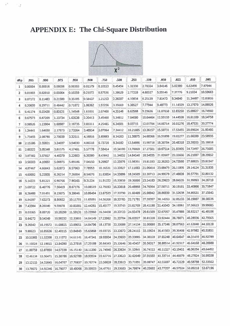
APPENDIX E: The Chi-Square Distribution

995 975 «950 750 = «500250

0.00098 0.00393

(5.02389 6.63490 7.87944

(0.10153 0.45494 1.32330

[ 1 | 0.00004

0.01003 (737776 9.21034

0.05064 0.10259 0.57536 1.38629 2.77259

0.07172 0.21580 0.35185 1.21253 9.34840

0.20699 0.48442 0.71072 /1,92256 | 1.14329 |

0.41174 1.14548 | 12,83250__

| 0.83121 -2.67460

1.63538 4.44938

16.0276

7 0.98926

-17.53455 20.09024

1.34441

2

3 4

5

6 0.67573 :

8

9 1.73493 / 19.0227 | 21.66599 10) 2.15586 3.24697

11 2.60322

44

12 3.07382

43° 3.56503 4.10692 5.00875

8.62873 7 17.11693. 14 4.07467 460092 6.26214 -18.24509

| 6.90766

5.6

6756419 18 6.26480

19 6.84397

20 7.43384

-35.47888 38.

/36.78071__ “21 8.03365

22 8.64272

9.26042

9.88623

| “40.64647 | 44.3

4192317 |

(4.46079 4 45.7229