Factors mediating structure and trophic interactions of ...

University of Windsor University of Windsor

Scholarship at UWindsor Scholarship at UWindsor

Electronic Theses and Dissertations Theses, Dissertations, and Major Papers

2012

Factors mediating structure and trophic interactions of estuarine Factors mediating structure and trophic interactions of estuarine

nekton communities nekton communities

Jill A. Olin University of Windsor

Follow this and additional works at: https://scholar.uwindsor.ca/etd

Recommended Citation Recommended Citation Olin, Jill A., "Factors mediating structure and trophic interactions of estuarine nekton communities" (2012). Electronic Theses and Dissertations. 5589. https://scholar.uwindsor.ca/etd/5589

This online database contains the full-text of PhD dissertations and Masters’ theses of University of Windsor students from 1954 forward. These documents are made available for personal study and research purposes only, in accordance with the Canadian Copyright Act and the Creative Commons license—CC BY-NC-ND (Attribution, Non-Commercial, No Derivative Works). Under this license, works must always be attributed to the copyright holder (original author), cannot be used for any commercial purposes, and may not be altered. Any other use would require the permission of the copyright holder. Students may inquire about withdrawing their dissertation and/or thesis from this database. For additional inquiries, please contact the repository administrator via email ([email protected]) or by telephone at 519-253-3000ext. 3208.

FACTORS MEDIATING STRUCTURE AND TROPHIC INTERACTIONS OF

ESTUARINE NEKTON COMMUNITIES

By

Jill A. Olin

A Dissertation Submitted to the Faculty of Graduate Studies

through Great Lakes Institute for Environmental Research in Partial Fulfillment of the Requirements for

the Degree of Doctor of Philosophy at the University of Windsor

Windsor, Ontario, Canada

2011

© 2011 Jill A. Olin

iii

CO-AUTHORSHIP DECLARATION

I hereby declare that this dissertation includes original research reprinted from co-

authored, submitted and published manuscripts. In all chapters A.T. Fisk contributed

intellectually by providing consultation, and facilities and materials required for

completion of the research. For chapter 2, P.W. Stevens, S.A. Rush and N.E. Hussey

contributed to the research with sample collection, statistical guidance and manuscript

consultation. For chapter 3, N.E. Hussey, M. Fritts, M.R. Heupel, C.A. Simpfendorfer

and G. Poulakis contributed to the research with sample collection, sample preparation

and consultation on the manuscript. For chapter 4, S.A. Rush and M.A. MacNeil

contributed to the research with statistical guidance and manuscript consultation. For

chapter 5, S.A. Rush and N.E. Hussey contributed to the research with statistical

guidance and manuscript consultation, M.R. Heupel, C.A. Simpfendorfer and G.R.

Poulakis contributed to the research with sample collection. The writing of all chapters

included in this dissertation, however, was completed entirely by the author, Jill A. Olin.

I am aware of the University of Windsor Senate Policy on Authorship and I

certify that I have properly acknowledged the contribution of other researchers to my

dissertation, and have obtained written permission from each of the co-author(s) to

include the above material(s) in my dissertation.

I certify that, with the above qualification, this dissertation, and the research to

which it refers, is the product of my own work.

iv

DECLARATION OF PREVIOUS PUBLICATION

This dissertation includes 3 original manuscripts that have been published or

submitted for publication in peer reviewed journals, as follows:

CHAPTER 2 Olin JA, Stevens PW, Rush SA, Hussey NE, Fisk AT. Loss of seasonal variability in nekton community structure in an altered tidal river: evidence for homogenization in a flow-altered system. (Manuscript in Review: Ecological Applications 17 October 2011). CHAPTER 3 Olin JA, Hussey NE, Fritts M, Heupel MR, Simpfendorfer CA, Poulakis

GR, Fisk AT. 2011. Maternal meddling in neonatal sharks: implications for interpreting stable isotopes in young animals. Rapid Communications in Mass Spectrometry 25:1008-1016.

CHAPTER 4 Olin JA, Rush SA, MacNeil MA, Fisk AT. 2011. Isotopic ratios reveal mixed seasonal variation among fishes from two subtropical estuarine systems. Estuaries and Coasts doi: 10.1007/s12237-011-9467-6

I certify that I have obtained a written permission from the copyright owner(s) to

include the above published material(s) in my dissertation. I certify that the above

material describes work completed during my registration as graduate student at the Great

Lakes Institute for Environmental Research, University of Windsor.

I declare that, to the best of my knowledge, my dissertation does not infringe upon

anyone’s copyright nor violate any proprietary rights and that any ideas, techniques,

quotations, or any other material from the work of other people included in my

dissertation, published or otherwise, are fully acknowledged in accordance with the

standard referencing practices. Furthermore, to the extent that I have included

copyrighted material that surpasses the bounds of fair dealing within the meaning of the

Canada Copyright Act, I certify that I have obtained a written permission from the

copyright owner(s) to include such material(s) in my dissertation.

v

I declare that this is a true copy of my dissertation, including any final revisions,

as approved by my dissertation committee and the Graduate Studies office, and that this

dissertation has not been submitted for a higher degree to any other University or

Institution.

vi

ABSTRACT

Understanding how communities and species assemblages persist is among the

most fundamental objectives in ecology, particularly as human modifications to the

landscape increase. Through application of traditional community metrics with emerging

biochemical tracers in combination with community/food web ecology theory, I provide

an evaluation of the effects of anthropogenically-altered freshwater flow disturbance on

estuarine nekton community structure and trophic interactions. These two parameters are

central toward understanding the functioning of aquatic communities and ensuring their

persistence.

This dissertation provides data regarding the effects of human-altered freshwater

flow on estuarine nekton communities in tidal rivers and, in doing so, has fostered

valuable findings regarding the application of stable isotopes to estuarine fishes and large

vertebrates. Specifically, this research demonstrates that losses of estuarine nekton

community biodiversity (Chapter 2), the shift in resource availability to lower trophic

level species (Chapter 5), and changes to energy flow pathways leading to higher trophic

level consumers (Chapter 6), are all associated with high flow events. This dissertation

further demonstrates that the application of stable isotopes requires consideration of a

species life history characteristics, as interpretation of a species diet and trophic roles can

be complex (Chapters 3 and 4).

Collectively, these findings suggest that high flow events affect the structure and

trophic interactions of estuarine nekton communities and provide a greater understanding

of the impacts of such anthropogenic-mediated stressors on these complex ecosystems.

Whether altered high-flow disturbance events result in adverse or beneficial effects on the

vii

persistence of estuaries remains to be established. However, in order to maintain and/or

restore the integrity of an ecosystem requires that conservation and management actions

be firmly grounded in scientific understanding. This becomes especially relevant as

worldwide changes to hydrologic connectivity continue with increasing anthropogenic

pressures.

This research demonstrates the potential for the simplification of food webs and

changes to dominant trophic assemblages that are associated with flow alteration. For the

commercially, recreationally and ecologically valuable species that define estuarine

nekton communities, these observations emphasize the necessity of research and

management programs aimed at maintaining the integrity of these highly-valued

ecosystems.

viii

DEDICATION

GBO, NAO and TJO

xoxo

ix

ACKNOWLEDGEMENTS

Many people have contributed to the completion of this dissertation, perhaps none

more than my supervisor Aaron Fisk. Aaron’s enthusiasm with the prospect of new

questions and ideas is invigorating and his patience is endless, even through my most

severe bouts of procrastination. Thank you, Aaron, for taking a chance and giving me this

opportunity.

I am extremely grateful to Nigel Hussey and Scott Rush for the many days spent

discussing ecological and stable isotope theory and ideas, no matter how absurd. Without

their guidance and support, I am certain that this dissertation would have been a lesser

version of itself. Their appetite for knowledge and desire to drink beer will remain an

inspiration to me for the rest of my career. I am grateful to Jim Peterson and Aaron

MacNeil for their guidance in helping me think more broadly, as especially outside of the

statistical box.

I thank Philip Stevens, Michelle Heupel, Colin Simpfendorfer, and Gregg

Poulakis for input and assistance with idea development and logistics of sample

collection. I thank my supervisory committee, Doug Haffner, Ken Drouillard and Daniel

Mennill, for their willingness to participate in this process and for their advice and

guidance throughout the course of this research.

I would also like to thank the staff of Mote Marine Laboratory’s Center for Shark

Research and of Florida Fish and Wildlife Conservation Commission’s, Port Charlotte

Field Station especially, Beau Yeiser, Tonya Wiley, Jack Morris, Jim Gelsleichter, John

Tyminski and Amy Timmers for keeping it light and fun on those long hot days searching

for sshaaarrks.

x

Much of this work would not have been completed without the efforts of Tom

Maddox, Mark Fritts, William Mark, Richard Doucette, David Qui, Nargis Ismail, Sandra

Ellis, Kristen Diemer, Amer Pasalic, Mary Lynn Mailloux, Carly Ziter and Jaclyn Brush.

Without each of you, I would still be in the lab processing samples. I thank Mary Lou

Scratch for being Mary Lou; your efforts do not go unnoticed.

I cherish my friendships with Michael Burtnyk, Bailey McMeans, Christina

Smeaton and Ryan Walter. Aside for my academic admiration for each of you, your

abilities to continually make me laugh and remind me of how important it is to do so,

made every moment of this adventure enjoyable. What stress?

I need to acknowledge my family and those that have stood behind me from the

start of this adventure. My parents have been tireless in their support for my adventures

(...and I have had many) and my success is entirely a result of their endless love and

support—and monetary subsidies from time to time. Ted deserves special credit for his

uncanny ability to make me see the bigger picture and refocus my compass- thank you

buddy. I thank my boys, Jacques and Finn for their unconditional love and snuggles. And

finally, I especially want to thank Gordon Paterson, for being that unwavering light at the

end of the tunnel. I am so blessed to have you in my life. Your passion and patience for

science is unmatched and it is contagious. Your support, even at distance, was a constant

reminder of why I embarked on this adventure. xx.

Let the next one begin!

xi

TABLE OF CONTENTS CO-AUTHORSHIP DECLARATION ............................................................................... iii DECLARATION OF PREVIOUS PUBLICATION .............................................................. iv ABSTRACT .................................................................................................................... vi DEDICATION .............................................................................................................. viii ACKNOWLEDGEMENTS ............................................................................................... ix LIST OF TABLES .......................................................................................................... xiv LIST OF FIGURES ....................................................................................................... xvii CHAPTER 1 - GENERAL INTRODUCTION .................................................................... 1 DISTURBANCE .................................................................................................... 2 ESTUARIES: ECOLOGY AND IMPORTANCE ...................................................... 4 STUDY SITES ...................................................................................................... 6 DISSERTATION OBJECTIVES ............................................................................. 7 OVERVIEW OF CHAPTERS ................................................................................. 9 REFERENCES . .......................................................................................................12 CHAPTER 2 - LOSS OF SEASONAL VARIABILITY IN NEKTON COMMUNITY STRUCTURE IN A TIDAL RIVER: EVIDENCE FOR HOMOGENIZATION IN A FLOW-ALTERED SYSTEM ....................................................................................................... 19 INTRODUCTION ................................................................................................ 20 MATERIALS AND METHODS ............................................................................ 23 Nekton community composition ................................................................. 24 Statistical analysis ..................................................................................... 26 RESULTS.............................................................................................................. . 29 Environmental parameters ........................................................................ 29 Nekton community: Trawl.......................................................................... 29 Nekton community: Seine .......................................................................... 31 Comparisons of nekton communities between estuaries ............................. 32 DISCUSSION ...................................................................................................... 33 Management implications .......................................................................... 38 REFERENCES .................................................................................................... 41 SUPPLEMENTAL MATERIAL ............................................................................ 55 CHAPTER 3 - MATERNAL MEDDLING IN NEONATAL SHARKS: IMPLICATIONS FOR INTERPRETING STABLE ISOTOPES IN YOUNG ANIMALS .......................................... 59 INTRODUCTION ................................................................................................ 60 MATERIALS AND METHODS ............................................................................ 63 RESULTS................................................................................................................ 65

xii

DISCUSSION ...................................................................................................... 67 REFERENCES .................................................................................................... 74 SUPPLEMENTAL MATERIAL ............................................................................ 83 CHAPTER 4 - ISOTOPIC RATIOS REVEAL MIXED SEASONAL VARIATION AMONG FISHES FROM TWO SUBTROPICAL ESTUARINE SYSTEMS ........................................ 85 INTRODUCTION ................................................................................................ 86 MATERIALS AND METHODS ............................................................................ 88 Sample collection ...................................................................................... 88 Stable isotope analysis .............................................................................. 89 Data Analysis ............................................................................................ 91 RESULTS................................................................................................................ 93 DISCUSSION ...................................................................................................... 95 Body size variability .................................................................................. 96 Seasonal variability ................................................................................... 98 Spatial variability .................................................................................... 100 Conclusions ................................................................................. ............101 REFERENCES.......................................................................................................102 SUPPLEMENTAL MATERIAL .......................................................................... 111 CHAPTER 5 - GOING WITH THE FLOW: REDUCED INTER-SPECIFIC VARIABILITY IN STABLE ISOTOPE RATIOS OF NEKTON IN RESPONSE TO ALTERED HIGH FLOW ... 114 INTRODUCTION .............................................................................................. 115 MATERIALS AND METHODS .......................................................................... 117 Study sites ............................................................................................... 117 Sample collection .................................................................................... 119 Stable isotope analysis ............................................................................ 120 Data analysis ....................................................................................... ...122 RESULTS.............................................................................................................. 123 DISCUSSION .................................................................................................... 125 Conclusions ............................................................................................. 132 REFERENCES .................................................................................................. 133 SUPPLEMENTAL MATERIAL .......................................................................... 149 CHAPTER 6 – CHANGES IN RESOURCE EXPLOITATION BY ESTUARINE CONSUMERS EXPERIENCING ALTERED HIGH FLOW AS INFERRED FROM FATTY ACID BIOMARKERS ................................................................................................... 151 INTRODUCTION .............................................................................................. 152 MATERIALS AND METHODS .......................................................................... 155 Study sites, species and sample collection ................................................ 155 Lipid and fatty acid analysis .................................................................... 157 Data analysis .......................................................................................... 158 RESULTS.............................................................................................................. 160 Fatty acids of consumers ......................................................................... 160 Variation in FA biomarkers of consumers in each trophic guild .............. 161 Ratios of ω3/ω6 PUFA ............................................................................ 163 DISCUSSION .................................................................................................... 163

xiii

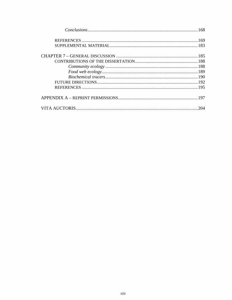
Conclusions ............................................................................................. 168 REFERENCES .................................................................................................. 169 SUPPLEMENTAL MATERIAL .......................................................................... 183 CHAPTER 7 – GENERAL DISCUSSION ..................................................................... 185 CONTRIBUTIONS OF THE DISSERTATION ..................................................... 188 Community ecology .............................................................................. 188 Food web ecology ................................................................................. 189 Biochemical tracers .............................................................................. 190 FUTURE DIRECTIONS ..................................................................................... 192 REFERENCES .................................................................................................. 195 APPENDIX A – REPRINT PERMISSIONS ................................................................... 197 VITA AUCTORIS....................................................................................................... 204

xiv

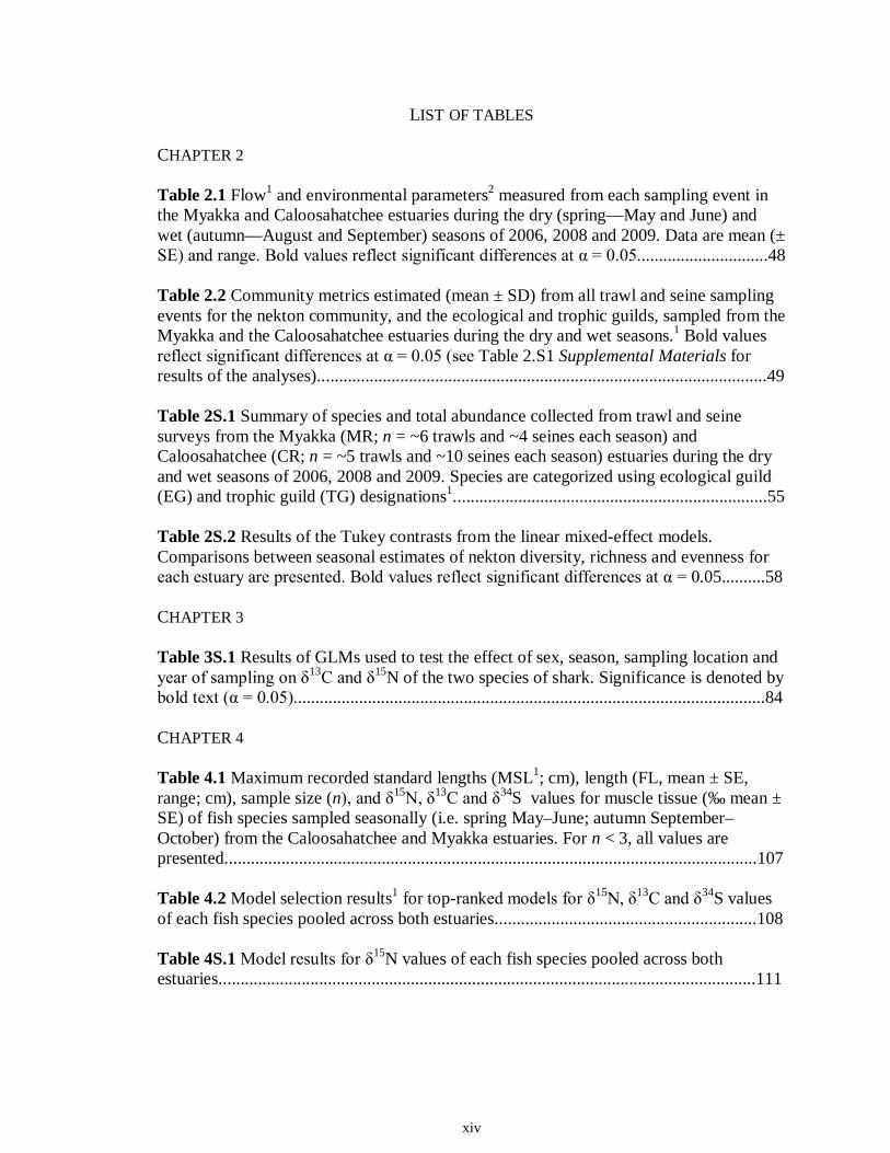
LIST OF TABLES CHAPTER 2 Table 2.1 Flow1 and environmental parameters2 measured from each sampling event in the Myakka and Caloosahatchee estuaries during the dry (spring—May and June) and wet (autumn—August and September) seasons of 2006, 2008 and 2009. Data are mean (± SE) and range. Bold values reflect significant differences at α = 0.05..............................48 Table 2.2 Community metrics estimated (mean ± SD) from all trawl and seine sampling events for the nekton community, and the ecological and trophic guilds, sampled from the Myakka and the Caloosahatchee estuaries during the dry and wet seasons.1 Bold values reflect significant differences at α = 0.05 (see Table 2.S1 Supplemental Materials for results of the analyses).......................................................................................................49 Table 2S.1 Summary of species and total abundance collected from trawl and seine surveys from the Myakka (MR; n = ~6 trawls and ~4 seines each season) and Caloosahatchee (CR; n = ~5 trawls and ~10 seines each season) estuaries during the dry and wet seasons of 2006, 2008 and 2009. Species are categorized using ecological guild (EG) and trophic guild (TG) designations1........................................................................55 Table 2S.2 Results of the Tukey contrasts from the linear mixed-effect models. Comparisons between seasonal estimates of nekton diversity, richness and evenness for each estuary are presented. Bold values reflect significant differences at α = 0.05..........58 CHAPTER 3 Table 3S.1 Results of GLMs used to test the effect of sex, season, sampling location and year of sampling on δ13C and δ15N of the two species of shark. Significance is denoted by bold text (α = 0.05)............................................................................................................84 CHAPTER 4 Table 4.1 Maximum recorded standard lengths (MSL1; cm), length (FL, mean ± SE, range; cm), sample size (n), and δ15N, δ13C and δ34S values for muscle tissue (‰ mean ± SE) of fish species sampled seasonally (i.e. spring May–June; autumn September–October) from the Caloosahatchee and Myakka estuaries. For n < 3, all values are presented..........................................................................................................................107 Table 4.2 Model selection results1 for top-ranked models for δ15N, δ13C and δ34S values of each fish species pooled across both estuaries............................................................108 Table 4S.1 Model results for δ15N values of each fish species pooled across both estuaries...........................................................................................................................111

xv

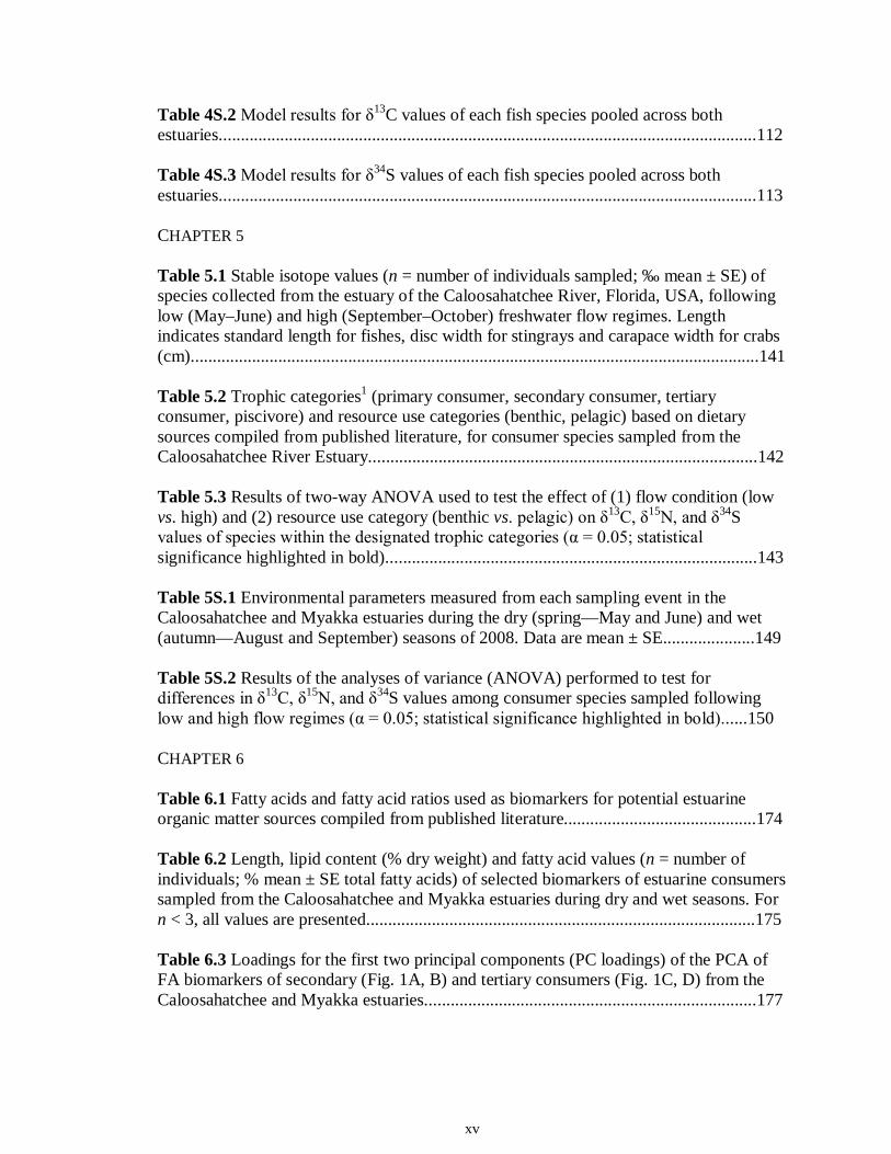
Table 4S.2 Model results for δ13C values of each fish species pooled across both estuaries...........................................................................................................................112 Table 4S.3 Model results for δ34S values of each fish species pooled across both estuaries...........................................................................................................................113 CHAPTER 5 Table 5.1 Stable isotope values (n = number of individuals sampled; ‰ mean ± SE) of species collected from the estuary of the Caloosahatchee River, Florida, USA, following low (May–June) and high (September–October) freshwater flow regimes. Length indicates standard length for fishes, disc width for stingrays and carapace width for crabs (cm)..................................................................................................................................141 Table 5.2 Trophic categories1 (primary consumer, secondary consumer, tertiary consumer, piscivore) and resource use categories (benthic, pelagic) based on dietary sources compiled from published literature, for consumer species sampled from the Caloosahatchee River Estuary.........................................................................................142 Table 5.3 Results of two-way ANOVA used to test the effect of (1) flow condition (low vs. high) and (2) resource use category (benthic vs. pelagic) on δ13C, δ15N, and δ34S values of species within the designated trophic categories (α = 0.05; statistical significance highlighted in bold).....................................................................................143 Table 5S.1 Environmental parameters measured from each sampling event in the Caloosahatchee and Myakka estuaries during the dry (spring—May and June) and wet (autumn—August and September) seasons of 2008. Data are mean ± SE.....................149 Table 5S.2 Results of the analyses of variance (ANOVA) performed to test for differences in δ13C, δ15N, and δ34S values among consumer species sampled following low and high flow regimes (α = 0.05; statistical significance highlighted in bold)......150 CHAPTER 6 Table 6.1 Fatty acids and fatty acid ratios used as biomarkers for potential estuarine organic matter sources compiled from published literature............................................174 Table 6.2 Length, lipid content (% dry weight) and fatty acid values (n = number of individuals; % mean ± SE total fatty acids) of selected biomarkers of estuarine consumers sampled from the Caloosahatchee and Myakka estuaries during dry and wet seasons. For n < 3, all values are presented.........................................................................................175 Table 6.3 Loadings for the first two principal components (PC loadings) of the PCA of FA biomarkers of secondary (Fig. 1A, B) and tertiary consumers (Fig. 1C, D) from the Caloosahatchee and Myakka estuaries............................................................................177

xvi

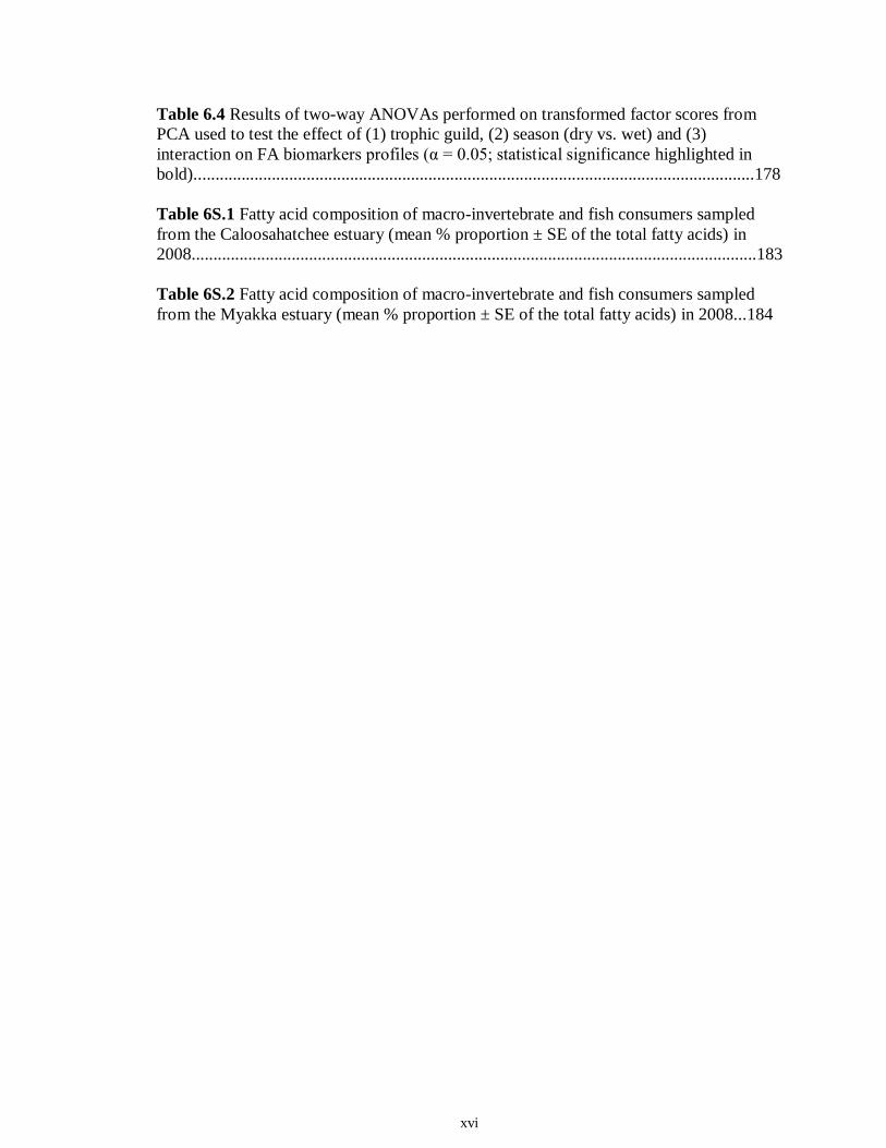
Table 6.4 Results of two-way ANOVAs performed on transformed factor scores from PCA used to test the effect of (1) trophic guild, (2) season (dry vs. wet) and (3) interaction on FA biomarkers profiles (α = 0.05; statistical significance highlighted in bold).................................................................................................................................178 Table 6S.1 Fatty acid composition of macro-invertebrate and fish consumers sampled from the Caloosahatchee estuary (mean % proportion ± SE of the total fatty acids) in 2008..................................................................................................................................183 Table 6S.2 Fatty acid composition of macro-invertebrate and fish consumers sampled from the Myakka estuary (mean % proportion ± SE of the total fatty acids) in 2008...184

xvii

LIST OF FIGURES CHAPTER 2 Figure 2.1 Map of the study sites showing the estuarine reaches of the Myakka and Caloosahatchee Rivers with respect to the south western coast of Florida.......................50 Figure 2.2 Mean daily river discharge recorded in the Caloosahatchee (black) and the Myakka (gray) from 2006 to 2010. River discharge data were obtained from the U.S. Geological Survey web site (http://water.usgs.gov/data.html) for the Myakka River at Myakka River near Sarasota (Station 02298830), and from the South Florida Water Management District web site (http://my.sfwmd.gov) for the Caloosahatchee River at the Cape Coral Bridge (Station CCORAL).............................................................................51 Figure 2.3 (A), (D) Nekton assemblage, (B), (E) ecological guild (estuarine species, black points; marine migrant species, gray points; freshwater species, white points) and (C), (F) trophic guild density from trawl sampling (primary consumers, black points; secondary consumers, gray points; tertiary consumers, white points) against season (data are mean density ± SE). Asterisks (*) indicates significant differences between dry and wet season at α = 0.05........................................................................................................52 Figure 2.4 (A), (D) Nekton assemblage, (B), (E) ecological guild (estuarine species, black points; marine migrant species, gray points; freshwater species, white points) and (C), (F) trophic guild density from seine sampling (primary consumers, black points; secondary consumers, gray points; tertiary consumers, white points) against season (data are mean density ± SE). Asterisks (*) indicates significant differences between dry and wet season at α = 0.05........................................................................................................53 Figure 2.5 Nonmetric multi-dimensional scaling (NMDS) depicting assemblage differences between the Myakka (dry: gray triangles; wet: gray circles) and Caloosahatchee (dry: black triangles; wet: black circles) estuaries. Data are density estimates of species collected via (A) trawl (stress: 0.12) and (B) seine (stress: 0.14), fitted with 95% confidence interval ellipses to represent the season-estuary differences. Strength of the environmental parameters is indicated in bold. Dotted lines represent the dry season and solid lines represent the wet season..........................................................54 CHAPTER 3 Figure 3.1 Relationships between USS and δ13C and δ15N values (mean ± SE) for (a), (b) muscle and (c), (d) liver of the Atlantic sharpnose (Rhizoprionodon terraenovae). Letters displayed above a given USS indicate the USS(s) for which pair-wise comparisons revealed significant differences. Numbers in plot (a) and (c) represent the sample size of sharks per USS...................................................................................................................79 Figure 3.2 Relationships between USS and δ13C and δ15N values (mean ± SE) for (a), (b) muscle and (c), (d) liver of the bull shark (Carcharhinus leucas). Letters displayed above

xviii

a given USS indicate the USS(s) for which pair-wise comparisons revealed significant differences. Numbers in plot (a) and (c) represent the sample size of sharks sampled per USS....................................................................................................................................80 Figure 3.3 Relationships between total length (TL) and δ13C and δ15N values for (a), (b) muscle and (c), (d) for liver tissues of the Atlantic sharpnose shark (Rhizoprionodon terraenovae) and (e), (f) for muscle and (g), (h) for liver of the bull shark (Carcharhinus leucas); curves were fitted with polynomial models.........................................................81 Figure 3.4 Changes in δ13C and δ15N values in regard to date sampled for (a), (b), muscle and (c), (d) for liver tissues of the Atlantic sharpnose shark (Rhizoprionodon terraenovae) and (e), (f) for muscle and (g), (h) for liver of the bull shark (Carcharhinus leucas); curves were fitted with polynomial models.........................................................82 CHAPTER 4 Figure 4.1 Map of the study site showing the locations of the Caloosahatchee and Myakka Rivers with respect to the south western coast of Florida. Insets: Locations of the estuarine portions of the two rivers from which fishes were sampled (black squares represent spring sample locations; gray circles represent autumn sample locations)....109 Figure 4.2 Parameter estimate results with 95% confidence intervals for the best-fit models for (A) δ15N, (B) δ13C and (C) δ34S values for each fish species sampled from the Caloosahatchee and Myakka estuaries. Symbols indicate species isotopic relationships were best described by season (●) or body size (□) where AIC c supported such an effect. Negative parameter estimates represent enriched isotopic values in autumn and positive parameter estimates represent depleted isotopic values in autumn. Trophic position1 is indicated along the y-axis for each species. 1Trophic position (TP) was estimated for all fishes using δ15N as follows: TP = TPbaseline + (δ15Nconsumer - δ15Nbaseline)/Δ15N, where TPbaseline is the estimated TP of the baseline organism, δ15Nconsumer and δ15Nbaseline are the mean δ15N of the consumer of interest and of the baseline organism, respectively, and 3.4‰ was used as the Δ15N (Post 2002). Mean δ15N of Mugil cephalus, designated as TP 2.0, was used as the baseline for all fishes, as this species is characterized as a primary consumer over the size range sampled here (Platell et al. 2006)...........................................................................................................110 CHAPTER 5 Figure 5.1 Map of the study site showing the location of the Caloosahatchee River with respect to the south-western coast of Florida. Inset: Indicates the sampling locations (e.g. water quality and consumer species; spring; ▲autumn) within the estuarine portion of the river............................................................................................................................144 Figure 5.2 Freshwater discharge (m3s1; black line) and salinity gradient (‰; grey line) for the Caloosahatchee estuary recorded daily from January to December of 2008.....145

xix

Figure 5.3 Mean (‰ ± 95% confidence interval) values of δ13C, δ15N and δ34S in consumer species sampled from the Myakka estuary following the dry (A), (C) and wet (B), (D) seasons...............................................................................................................146 Figure 5.4 Mean (‰ ± 95% confidence interval) values of δ13C, δ15N and δ34S in consumer species sampled from the Caloosahatchee estuary following the dry (A), (C) and wet (B), (D) seasons.................................................................................................147 Figure 5.5 Mean (‰ ± SE) values of (A) δ13C, (B) δ15N and (C) δ34S depicting differences between flow regimes (● low flow; ○ high flow) in consumer species sampled from the Caloosahatchee River estuary. Significant differences in isotopic values between regimes, based on ANOVA, are highlighted in gray (α = 0.05).......................148 CHAPTER 6 Figure 6.1 Principal component analyses of the secondary consumers depicting seasonal differences using FA. Ellipses are one standard deviation around the mean of each consumer’s biomarker profile given the season (closed symbols and black lines represent dry season; open symbols and gray lines represent wet season). Only biomarkers with the strongest contribution to principal components are depicted (Table 6.3).......................179 Figure 6.2 Principal component analyses of the tertiary consumers depicting seasonal differences using FA biomarkers. Ellipses are one standard deviation around the mean of each consumer’s biomarker profile given the season (closed symbols and black lines represent dry season; open symbols and gray lines represent wet season). Biomarkers with the strongest contribution to principal components are depicted (Table 6.3)........180 Figure 6.3 Seasonal mean ± SE % FA biomarkers of total lipids of Carcharhinus leucas (black bars represents dry season; white bars represents wet season). Significant differences between seasons are indicated by asterisks (P < 0.05)..................................181 Figure 6.4 Ratio of ω3/ω6 FA (mean ± SE) in consumer species sampled following dry (black) and wet (white) season of the (A) Caloosahatchee and (B) Myakka estuaries. Dotted lines represent overall mean of ratios for each season (black represents dry; gray represents wet). Asterisk indicates significant one-way ANOVA at α = 0.05................182

1

CHAPTER 1

GENERAL INTRODUCTION

2

The food web is one of the central and unifying concepts in ecology (Lindeman

1942; Martinez 1995) representing an integration of all ecological relationships within a

community (Elton 1927). The food web concept provides the framework to test and

quantify ecosystem processes such as population dynamics, predator - prey relationships,

feeding ecology, and responses to disturbance. Food webs are modeled on the unifying

theory of energy transfer (Lindeman 1942) which provides a mechanism for

characterizing the trophic interactions and exchanges within and between communities

(Odum 1968). As such, understanding the factors regulating food web structure is critical.

This is especially relevant in aquatic food webs, where species extinction rates are

increasing as a result of multiple anthropogenic stresses (Ricciardi and Rasmussen 1999;

Jackson et al. 2001).

DISTURBANCE

Periodic disturbances are a natural component of nearly all ecosystems and are

important determinants of community structure and dynamics (Sousa 1984; Pickett and

White 1985). A disturbance as defined by Pickett and White (1985) is a relatively

discrete event in time that disrupts community or population structure, and changes

resource availability or the nature of the physical environment.

Some ecological models predict that species mortalities as imposed by occasional

natural disturbances, such as fires, are integral components of most ecosystems and can

be vital for maintaining biological diversity as well as renewing essential nutrients

(Pickett and White 1985; Webster and Halpern 2010). However, many of these same

models also predict a decrease in diversity when the frequency or severity in magnitude

3

of the disturbance is too great (intermediate disturbance hypothesis; Connell 1978). In

aquatic systems, this is best illustrated by drought and storm events, where reductions in

species complexity i.e., decrease in diversity, in stream (Walters and Post 2011),

estuarine (Livingston et al. 1997; Greenwood et al. 2006; Baptista et al. 2010) and coastal

marine (Byrnes et al. 2011) communities have been documented to coincide with these

events. Understanding how such reductions in diversity impact community functioning is

critical for regulating anthropogenic-mediated effects of habitat degradation (Mora et al.

2007), urbanization (Marchetti et al. 2006), species invasions (Lodge 1993) and species

overexploitation (Pauly et al. 1998). This is especially relevant as climate change models

predict increased frequency and severity of many forms of large abiotic disturbances,

such as tropical storms (Easterling et al. 2000; Meehl et al. 2000). As such, simplification

of food webs is an expected consequence.

Recently, it has been argued that some of the most fundamental aspects behind the

persistence and functioning of complex systems may be manifested in their ability to

adapt in the face of disturbance (Levin 1998). McCann and Rooney (2009) argue that

temporal and spatial variability in food web structure and the ability of species to rapidly

respond to such variation are critical to the persistence of food webs. McCann (2007)

and McCann and Rooney (2009) advocate the empirical examination of food web

variability by evaluating how communities, specifically those with relatively consistent

species assemblages, respond and/or change across resource gradients in natural and

anthropogenic altered systems. Such evaluations will enable predictions regarding the

consequences of human modifications on the structure and functioning of ecosystems

(McCann 2007). In this manner, food web dynamics are fundamentally based on the

4

premise of predicting species interactions and thereby understanding predator-prey

relationships. This permits the ability to determine the magnitude of energy available to a

consumer and also facilitates an understanding of the extent of resource exploitation that

may be influenced by disturbance events. The loss of individual species and subsequent

biodiversity is known to impact the functioning of both organisms and ecosystems

(Cardinale et al. 2006). Should natural or anthropogenic-mediated disturbance events

function similarly to alter species abundance and diversity, such changes can lead to

significant impairments to ecosystem structure and functioning (McCann and Rooney

2009). Given the increasing frequency of anthropogenic-mediated disturbances such as

species invasions, habitat loss and climate change, there is a need to understand how

species and ecosystems respond to such events (McCann 2000).

ESTUARIES: ECOLOGY AND IMPORTANCE

Cowardin et al. (1979) formally defined estuaries as “deep-water tidal habitats

and adjacent tidal wetlands which are usually semi-enclosed by land, but have open,

partially obstructed, or sporadic address to the open ocean and in which water is at least

occasionally diluted by freshwater runoff from the land.” As such, estuaries are thus

viewed as transition zones between terrestrial, and freshwater and marine aquatic systems

(Dardeu et al. 1992). This confluence of freshwater and marine aquatic environments

results in a wide spectrum of abiotic and biotic characteristics that influence estuarine

physical and biological community structure (Dardeu et al. 1992; Rush et al. 2010).

Consequently, estuaries are valued as highly productive environments that provide

important spawning, nursery, refuge and foraging habitats for a number of species,

5

including commercial and recreational fishes during one or more of their life history

stages (Beck et al. 2001). For example, a recent estimate of U.S. fisheries indicated that

approximately 46% of the commercial and 80% of the recreational fisheries harvests are

derived from the communities of Gulf Coast estuaries (Lellis-Dibble et al. 2008).

Estuaries, however, are among the most intensely modified ecosystems as a

consequence of extensive hydrological alteration, habitat alteration and chemical and

organic pollution (Lotze et al. 2006). Globally, there are few estuarine systems that

remain unaffected by upstream manipulation of their freshwater flow (Dynesius and

Nilsson 1994; Nilsson et al. 2005). River regulation by dams has fragmented hydrological

and ecological processes (Nilsson et al. 2005) often restricting or severing connectivity to

estuaries and coastal marine systems, as well as facilitating the introduction and

establishment of invasive species which can modulate flows of energy and nutrients

(Bunn and Arthington 2002). Such anthropogenic-mediated alterations can be detrimental

to downstream communities, as freshwater inflow from riverine sources provides

nutrients, sediment and organic matter essential for primary and secondary production in

these systems (Mallin et al. 1993; Chanton and Lewis 2002).

Anthropogenic-mediated alterations to freshwater flow indirectly affect the

physicochemical characteristics of the system by shifting the salinity and dissolved

oxygen gradients, and increasing turbidity, among other impacts (Sklar and Browder

1998; Gillson 2011). Predicting the response of estuaries to changing environmental

conditions is challenging, as it necessitates understanding interactions among several

trophic levels and among multiple nutrient sources (Rush et al. 2010). Many life-history

stages of estuarine species from juveniles to adult are intimately tied to water flow (Bunn

6

and Arthington 2002; Rehage and Trexler 2006). For example, larval stages of many

estuarine fishes are reliant on freshwater flow as a cue for migration into estuaries

(Strydom et al. 2002; Gillanders et al. 2011). Thus, disruption of this natural event affects

recruitment, and thus growth and mortality of these species (Purtlebaugh and Allen

2010). Consequently, the effects of altered flow on estuarine communities are expected to

be revealed not only by the presence or absence of certain species (Hofmann and Powell

1998) but also by changes in food web interactions (Akin et al. 2005).

STUDY SITES

The Charlotte Harbor Estuary is a large (~700 km2) relatively shallow estuary on

the southwest coast of Florida that serves as a forage and/or nursery area for more than

255 species of resident, migrant, recreational and commercial fishes of the Gulf of

Mexico (Poulakis et al. 2004), as well as to federally-protected species (e.g., manatees,

sea turtles and dolphins). The Caloosahatchee and Myakka Rivers (see Figure 2.1; details

on the study areas can be found in the following chapters) are major tributaries of

Charlotte Harbor Estuary. These rivers are subject to different anthropogenic influences,

regarding land-use development, shoreline modification and freshwater flow.

Specifically, the Myakka River has been subjected to relatively minor anthropogenic

modifications and experiences relatively natural flow regimes. In contrast, the artificial

connection of Lake Okeechobee to the Caloosahatchee River represents a unique

anthropogenic manipulation of riverine hydrology (Doering and Charmberlain 1998),

whereby substantial seasonal discharge from Lake Okeechobee occurs for flood control

and water supply, as well as to flush algal blooms and salt water intrusion (Flaig and

7

Capece 1998). Accompanying these hydrologic changes is a decrease in water quality,

marked by increases in turbidity and nutrient loading, changes in water residence time in

the estuary, and alteration in the natural salinity gradient (Barnes 2005). These flow

characteristics of the Caloosahatchee and Myakka provide a unique opportunity to test

how disturbance, in the form of altered flow regimes, affects food webs and provides the

context by which this dissertation was developed.

DISSERTATION OBJECTIVES

The objective of this dissertation was to apply the principles and foundations of

community/food web ecology to understanding estuarine community response to

anthropogenically-altered freshwater flow disturbance. Patterns of community response

to flow variability were investigated in a framework that encompassed both temporal and

spatial scales and addressed changes in community characteristics associated with a

human-driven disturbance. Specifically, this dissertation investigates the effects of altered

freshwater flow on community structure and trophic interactions of estuarine

communities by comparing the Myakka and Caloosahatchee Rivers and their contrasting

flow regimes.

To investigate the effects of altered flow disturbance on estuarine communities, I

applied a combination of traditional community metrics with biochemical tracers to

demonstrate how altered vs. natural flow affect temporal estuarine community structure

and function. Traditional metrics included estimates of species density, diversity,

richness, and evenness. The biochemical tracers included stable isotopes of carbon

(δ13C), nitrogen (δ15N) and sulfur (δ34S), and fatty acid biomarkers.

8

Application of biochemical tracers, especially stable isotopes and fatty acids, have

become increasingly prevalent for investigations of diet, trophic interactions and foraging

habitats (Peterson and Fry 1987; Iverson et al. 1997; Post et al. 2000; Rubenstein and

Hobson 2004) which has allowed for broad evaluation and inference regarding the

changing structure and function of food webs (Vander Zanden et al. 1999; Hebert et al.

2006). The stable isotope approach is based on the fact that the ratios of the stable

isotopes of nitrogen (15N/14N), carbon (13C/12C) and sulfur (34S/32S) in consumers’ tissues

reflect (1) isotopic composition of their dietary resources and (2) isotopic fractionation

during diet assimilation (DeNiro and Epstein 1978, 1981). Enrichment of isotopes within

tissues of a consumer over that of its diet arises as a result of the greater retention of the

heavier over the lighter isotope during the process of protein amination and deamination

for 15N and 34S, and respiration for 13C (DeNiro and Epstein 1978; 1981). This produces

ratios in a consumer’s tissues, between approximately 0 and 2‰ for δ13C and δ34S, and 2

and 5‰ for δ15N, higher than those of its diet (DeNiro and Epstein 1981; Minagawa and

Wada 1984; Post 2002; Vanderklift and Ponsard 2003). Specifically, δ15N values have

found application in determining the relative trophic position of a consumer (Minagawa

and Wada1984; Post 2002), and δ13C and δ34S values have found application in

determining basal organic matter sources incorporated into a consumer’s diet (Peterson

and Fry 1987), species habitat use (Herzka 2005) and dependence on marine and/or

terrestrial/freshwater energy pathways (Simenstad and Wissmar 1985; Darnaude et al.

2004; McLeod and Wing 2009).

Fatty acids are the main constituents of many types of lipid and are required for

normal growth and development of an organism (Arts 1999). Essential fatty acids are

9

fatty acids that cannot be efficiently synthesized by consumers in amounts sufficient for

optimal growth and development, instead originate in primary producers and need to be

acquired through diet (Arts et al. 2001). The utility of fatty acids as biochemical tracers

of food web pathways stems from the fact that they are highly conserved during trophic

interactions (Iverson et al. 2004) and incorporated into consumers’ tissue in largely

unmodified form (Falk-Peterson et al. 2002; Hall et al. 2006), thereby allowing

inferences to be made regarding consumer diet composition (Iverson et al. 2004; Hebert

et al. 2009). For example, the ratio of ω3/ω6 polyunsaturated fatty acids (PUFA) is a

useful indicator of the relative contribution of aquatic vs. terrestrial-derived resources in a

consumers’ diet (Smith et al. 1996; Hebert et al. 2009).

OVERVIEW OF CHAPTERS

In Chapter 2 (Loss of seasonal variability in nekton community structure in a tidal

river: evidence for homogenization in a flow-altered system), I evaluated seasonal trends

(i.e., the transition of dry to wet season) of estuarine nekton trawl and seine assemblages

from the Myakka and Caloosahatchee estuaries, with the prediction that the these

estuaries would exhibit contrasting responses to the onset of the wet season, i.e., the

Caloosahatchee Estuary would exhibit loss in diversity, whereas the Myakka would

exhibit an increase. By comparing, nekton density, diversity, richness, and evenness

within and between estuaries, this chapter provides unique evidence regarding nekton

community response to altered high-flow. This chapter provides a baseline by which

hypotheses in subsequent chapters regarding effects of high-flow on the nekton

community were posed.

10

Stable isotope analysis has proven to be a powerful tool for the study of estuarine

food webs (Peterson and Fry 1987). Despite the prevalence of stable isotope analyses in

ecological studies of diet and food webs, there are still a number of confounding factors

that can complicate interpretations of stable isotope data and studies have recommended

establishing species-specific criteria for accurate isotopic assessment of an organism

(Sweeting et al. 2007). I tested assumptions regarding (1) tissue stable isotope values of

young individuals reflecting their current diet and (2) estuarine fishes exhibiting

ontogenetic or body-size based shifts in dietary resources. In this manner, Chapter 3 and

Chapter 4 allowed me to determine whether a species, sampled over variable time periods

and over a range of sizes, would be suitable for use in subsequent community analyses,

without confounding size-based effects.

In Chapter 3 (Maternal meddling in neonatal sharks: implications for interpreting

stable isotopes in young animals), I examined the relationships between several size

metrics and stable isotope values of δ13C and δ15N measured from muscle and liver

tissues of two species of placentatrophic shark to determine the length of time tissues of

young individuals are influenced by their mothers’ isotopic signal. This chapter provides

guidance regarding estimation of trophic position and characterization of carbon sources

and diet of young sharks using stable isotopes.

In Chapter 4 (Isotopic ratios reveal mixed seasonal variation among fishes from

two subtropical estuarine systems), I examined temporal and spatial relationships

between body size and δ15N, δ13C and δ34S values for fish species across multiple trophic

levels, with the expectation that temporal variability would be manifested in changes to

δ13C and δ34S with season, and that δ15N would scale with body size. This chapter

11

supports previous observations in estuarine fishes regarding body size and in that context

allows for inclusion of estuarine fishes in subsequent food web analyses.

In Chapter 5 (Going with the flow: reduced inter-specific variability in stable

isotope ratios of nekton in response to altered high flow), I evaluated the effect of altered

high-flow on food web structure by comparing seasonal isotopic trends (δ13C, δ15N and

δ34S) in consumer species sampled over four trophic levels in the Caloosahatchee and

Myakka estuaries. From the community perspective, I hypothesized that extreme high

flows would be most evident among lower trophic level species (i.e., primary and

secondary consumers). Specifically, we expected species sampled following the dry

season to be enriched in 13C and 34S relative to those sampled following the wet season,

reflecting a polyhaline estuarine status (i.e., tidally influenced). In contrast, those

sampled following the wet season would be depleted in 13C and 34S reflective of an

oligohaline estuarine status (i.e., terrestrial/freshwater influenced). Additionally, the

magnitude in the seasonal isotopic shifts would be expected to be greater in the

Caloosahatchee as opposed to the Myakka. This chapter demonstrates the effect that

altered high flow has on isotopic values of consumer species and in so doing,

demonstrates the effect on the overall food web structure, regarding relative trophic

position and carbon resources of estuarine consumers.

In Chapter 6 (Changes in resource exploitation by estuarine consumers in response to

altered high flow as inferred from fatty acid biomarkers), I used fatty acid biomarkers to

evaluate the main trophic pathways and relative importance of different energy sources to

the diet of estuarine consumers under different flow regimes. I hypothesized that the

contribution of allochthonous carbon sources (i.e., terrestrially-derived) would be more

12

important during the wet season than the dry season and would be especially evident

during extreme high flow. Fatty acid biomarkers and specific fatty acid ratios (i.e.,

ω3/ω6) indicative of marine vs. terrestrial/freshwater resource use were measured in

species that constitute several trophic guilds, sampled seasonally from both estuaries.

This chapter provides a novel application of fatty acid biomarkers to track altered flow

events in estuaries and provides a compliment to Chapter 5, for determining flow-related

changes to carbon source and energy pathways of estuarine consumers.

In light of escalating human water demand, urbanization, and climate change that

will ultimately lead to increased frequency of extreme flow events, in chapter 7, I

summarize the chapters presented here and discuss their contribution to understanding of

how altered flow effects estuarine nekton communities in the context of maintaining

structure and stability of these productive systems.

REFERENCES

Akin S., Buhan E., Winemiller K.O. & Yilmaz H. 2005. Fish assemblage structure of Koycegiz Lagoon-estuary, Turkey: Spatial and temporal distribution patterns in relation to environmental variation. Estuarine, Coastal and Shelf Science 64:671–684. Arts M.T., Ackman R.G. & Holub B.J. 2001. ‘Essential fatty acids’ in aquatic ecosystems: a crucial link between diet and human health and evolution. Canadian Journal of Fisheries and Aquatic Sciences 58:122–137. Arts M.T. 1999. Lipids in freshwater zooplankton: selected ecological and physiological aspects. In: Lipids in Freshwater Ecosystems (M.T. Arts and B.C. Wainman, Eds.). Springer Verlag, New York. Baptista J., Martinho F., Dolbeth M., Viegas I., Cabral H. & Pardal M. 2010. Effects of freshwater flow on the fish assemblage of the Mondego estuary (Portugal): comparison between drought and non-drought years. Marine and Freshwater Research 6: 490–501. Barnes T. 2005. Caloosahatchee Estuary conceptual ecological model. Wetlands 25:884–897.

13

Beck M.W., Heck K.L., Able K.W., Childers D.L., Eggleston D.B., Gillanders B.M., Halpern B., Hays C.G., Hoshino K., Minello T.J., Orth R.J., Sheridan P.F. & Weinstein M.P. 2001. The identification, conservation and management of estuarine and marine nurseries for fish and invertebrates. Bioscience 51:633–641. Bunn S.E. & Arthington A.H. 2002. Basic principles and ecological consequences of altered flow regimes for aquatic biodiversity. Environmental Management 30:492–507. Byrnes J.E., Reed D.C, Cardinale B.J., Cavanaugh K.C, Holbrook S.J. & Schmitt R.L. 2011. Climate-driven increases in storm frequency simplify kelp forest food webs. Global Change Biology 17:2513–2524. Cardinale B.J., Srivastava D.S., Duffy J.E., Wright J.P., Downing A.L., Sankaran M. & Jouseau C. 2006. Effects of biodiversity on the functioning of trophic groups and ecosystems. Nature 443:989–92. Chanton J. & Lewis F.G. 2002. Examination of coupling between primary and secondary production in a river-dominated estuary: Apalachicola Bay, Florida, USA. Limnology and Oceanography 47:683–697. Connell J.H. 1978. Diversity in tropical rain forests and coral reefs - high diversity of trees and corals in maintained only in a non-equilibrium state. Science 199:1302–1310. Cowardin L.M., Carter V., Golet F.C. & LaRoe E.T. 1979. Classification of wetlands and deepwater habitats of the United States. U. S. Department of the Interior, Fish and Wildlife Service Office of Biological Services, Jamestown, ND. Technical Report: FWS/OBS/79-31:1–103. Dardeu M.R., Modlin R.F., Schroeder W.W. & Stout J.P. 1992. Estuaries. In: Biodiversity of the Southeastern United States: Aquatic Communities. (C.T. Hackney, S.M. Adams, and W.H. Martin, Eds.). pp. 614−744. John Wiley and Sons, Inc. New York, NY, USA. Darnaude A.M., Salen-Picard C., Polunin N.V.C. & Harmelin-Vivien M.L. 2004. Trophodynamic linkages between river runoff and coastal fishery yield elucidated by stable isotope data in the Gulf of Lions (NW Mediterranean). Oecologia 138:325–332. DeNiro M.J. & Epstein S. 1978. Influence of diet on the distribution of carbon isotopes in animals. Geochimica et Cosmochimica Acta 42:495–506. DeNiro M.J. & Epstein S. 1981. Influence of diet on the distribution of nitrogen isotopes in animals. Geochimica et Cosmochimica Acta 45:341–351. Doering P.H. & Chamberlain R.H. 1998. Water quality in the Caloosahatchee Estuary, San Carlos Bay and Pine Island Sound. In: Proceedings of the Charlotte Harbor Public

14

Conference and Technical Symposium, Technical Report No. 98-02, Charlotte Harbor National Estuary Program, Punta Gorda, FL, pp. 229–240. Dynesius M. & Nilsson C.1994. Fragmentation and flow regulation of river systems in the northern 3rd of the world. Science 266:753–762. Easterling D.R., Meehl G.A., Parmesan C., Changnon S.A., Karl T.R. & Mearns L.O. 2000. Climate Extremes: Observations, Modeling, and Impacts. Science 289:2068–2074. Elton C. (1927). Animal Ecology. Sidgwick & Jackson, Ltd., London. Falk-Petersen S., Haug T., Nilssen K.T., Wold A. & Dahl T.M. 2004. Lipids and trophic linkages in harp seal (Phoca groenlandica) from the eastern Barents Sea. Polar Research 23:43–50. Flaig E.G. & Capece J. 1998. Water use and runoff in the Caloosahatchee watershed. In: Proceedings of the Charlotte Harbor Public Conference and Technical Symposium, Technical Report No. 98-02, Charlotte Harbor National Estuary Program, Punta Gorda, FL, pp. 73–80. Gillson J. 2011. Freshwater flow and fisheries production in estuarine and coastal systems: Where a drop of rain is not lost. Reviews in Fisheries Science 19:168–186. Gillanders B.M., Elsdon T.S., Halliday I.A., Jenkins G.P., Robins J.B. & Valesini F.J. 2011. Potential effects of climate change on Australian estuaries and fish utilizing estuaries: a review. Marine and Freshwater Research 62:1115–1131. Greenwood M.F.D., Stevens P.W. & Matheson R.E. 2006. Effects of the 2004 Hurricanes on the fish assemblages in two proximate southwest Florida estuaries: Changes in the context of inter-annual variability. Estuaries and Coasts 29:985–996. Hall D., Lee S.Y. & Mezaine T. 2006. Fatty acids as trophic tracers in an experimental estuarine food chain: tracer transfer. Journal of Experimental Marine Biology and Ecology 336:42–53. Hebert C.E., Weseloh D.V., Gauthier L.T., Arts M.T. & Letcher R.J. 2009 Biochemical tracers reveal intra-specific differences in the food webs utilized by individual seabirds. Oecologia 160:15–23. Hebert C.E., Arts M.T. & Weseloh D.V.C. 2006. Ecological tracers can quantify food web structure and change. Environmental Science and Technology 40:5618–5623. Herzka S.Z. 2005. Assessing connectivity of estuarine fishes based on stable isotope ratio analysis. Estuarine, Coastal and Shelf Science 64:58–69. Hoffman E.E. & Powell T.M. 1998. Environmental variability effects on marine fisheries: four cases histories. Ecological Applications 8:S23–S32.

15

Iverson S.J., Field C., Bowen W.D. & Blanchard W. 2004. Quantitative fatty acid signature analysis: a new method of estimating predator diets. Ecological Monographs 74:211–235. Iverson S.J., Frost K.J. & Lowry L.L. 1997. Fatty acid signatures reveal fine scale structure of foraging distribution of harbor seals and their prey in Prince William Sound, Alaska. Marine Ecology Progress Series 151:255–271. Jackson J.B.C., Kirby M.X., Bereger K., Bjorndal K.A., Botsford L.W., Bourque B.J., Bradbury R.H., Cooke R., Erlandson J., Estes J.A., Hughes T.P., Kidwell S., Lange C.B., Lenihan H.S., Pandolfi J.M., Peterson C.H., Steneck R.S., Tegner M.J. & Warner R.R. 2001. Historical overfishing and the recent collapse of coastal ecosystems. Science 27: 629–637. Lellis-Dibble K.A., McGlynn K.E. & Bigford T.E. 2008. Estuarine Fish and Shellfish Species in U.S. Commercial and Recreational Fisheries: Economic Value as an Incentive to Protect and Restore Estuarine Habitat. U.S. Dept. Commerce, NOAA Tech. Memo. NMFSF/SPO-90, 94 p. Levin S.A. 1998. Ecosystems and the biosphere as complex adaptive systems. Ecosystems 1:431–436. Lindeman R.L. 1942. The trophic-dynamic aspect of ecology. Ecology 23:399–417. Livingston R.J., Niu X., Lewis G. & Woodsum G.C. 1997. Freshwater input to a gulf estuary: long-term control of trophic organization. Ecological Applications 7:277–299. Lodge D.M. 1993. Species invasions and deletions. In: Biotic Interactions and Global Change (P.M. Kareiva, J.G. Kingsolver and R.B. Hney, Eds.), pp. 367–387. Sunderland, Massachusetts. Lotze H.K., Lenihan H.S., Bourque B.J., Bradbury R.H., Cooke R.G., Kay M.C., Kidwell S.M., Kirby M.X., Peterson C.H. & Jackson J.B.C. 2006. Depletion, degradation, and recovery potential of estuaries and coastal seas. Science 312:1806–1809. Mallin M.A., Paerl H.W., Rudek J. & Bates P.W. 1993. Regulation of primary production by watershed rainfall and river flow. Marine Ecology Progress Series 93:199–203. Marchetti M.P., Lockwood J.L. & Light T. 2006. Effects of urbanization on California’s fish diversity: Differentiation, homogenization and the influence of spatial scale. Biological Conservation 127:310–318. Martinez N.D. 1995. Unifying ecological sub-disciplines within ecosystems food webs. In: Linking species and ecosystems (J. H. Lawton and C. Jones, Eds.), pp. 166–175. Chapman and Hall, New York, New York, USA.

16

Meehl G.A., Zwiers F., Evans J., Knutson T., Mearns L. & Whetton P. 2000. Trends in extreme weather and climate events: issues related to modeling extremes in projections of future climate change. Bulletin of the American Meteorological Society 81:427–436. McCann K.S. & Rooney N. 2009. The more food webs change, the more they stay the same. Philosophical Transactions of the Royal Society B 364:1789–1801. McCann K.S. 2007. Protecting biostructure. Nature 446:29. McCann K.S. 2000. The diversity-stability debate. Nature 405:228–233. McLeod R.J. & Wing S.R. 2009. Strong pathways for incorporation of terrestrially derived organic matter into benthic communities. Estuarine, Coastal and Shelf Science 82:645–653. Minagawa M. & Wada E. 1984. Stepwise enrichment of 15N along food chains: further evidence and the relation between δ15N and animal age Geochimica et Cosmochimica Acta 48:1135–1140. Mora C., Metzker R., Rollo A. & Myers R.A. 2007. Experimental simulations about the effects of habitat fragmentation and overexploitation on populations facing environmental warming. Proceedings of the Royal Society B 274:1023–1028. Nilsson C., Reidy C.A, Dynesius M. & Revenga C. 2005. Fragmentation and flow regulation of the world’s large river systems. Science 308:405–408. Odum E.P. 1968. Energy flow in ecosystems: A historical review. American Zoologist 8: 11–18. Pauly D., Christensen V., Dalsgaard J., Froese R. & Torres F. 1998. Fishing down marine food webs. Science 279:860–863. Peterson B.J. & Fry B. 1987. Stable isotopes in ecosystem studies. Annual Review of Ecology, Evolution and Systematics 18:293–320. Pickett S.T.A. & White P.S. 1985. Patch dynamics: a synthesis. In: The ecology of natural disturbance and patch dynamics (S.T.A. Pickett and P.S. White, Eds.), pp. 371–384. Academic Press, New York. Post D.M. 2002. Using stable isotopes to estimate trophic position: models, methods and assumptions. Ecology 83:703–718. Post D.M., Conners M.E. & Goldberg D.S. 2000. Prey preference by a top predator and the stability of linked food chains. Ecology 81:8–14.

17

Poulakis G.R., Matheson R.E., Mitchell M.E., Blewett D.A. & Idelberger C.F. 2004. Fishes of the Charlotte Harbor estuarine system, Florida. Gulf of Mexico Science 2:117–150. Purtlebaugh C.H. & Allen M.S. 2010. Relative Abundance, Growth, and Mortality of Five Age-0 Estuarine Fishes in Relation to Discharge of the Suwannee River, Florida. Transactions of the American Fisheries Society 139:1233–1246. Rehage J.S. & Trexler J.C. 2006. Assessing the net effect of anthropogenic disturbance on aquatic communities in wetlands: community structure relative to distance from canals. Hydrobiologia 569:359–373. Ricciardi A. & Rasmussen J.B. 1999. Extinction rates of North American freshwater fauna. Conservation Biology 13:1220–1222. Rubenstein D.R. & Hobson K.A. 2004. From birds to butterflies: animal movement patterns and stable isotopes. Trends in Ecology and Evolution 19:256–263. Rush S.A., Olin J.A., Fisk A.T., Woodrey M.S. & Cooper R.J. 2010. Trophic relationships of a marsh bird differ between Gulf Coast estuaries. Estuaries and Coasts 33: 963–970. Simenstad C.A. & Wissmar R.C. 1985. δ13C evidence of the origins and fates of organic carbon in estuarine and nearshore food webs. Marine Ecology Progress Series 22:141–152. Sklar F.H. &Browder J.A. 1998. Coastal environmental impacts brought about by alterations to freshwater flow in the Gulf of Mexico. Environmental Management 22:547–562. Smith R.J., Hobson K.A., Koopman H.N. & Lavigne D.M. 1996. Distinguishing between populations of fresh- and salt-water harbor seals (Phoca vitulina) using stable isotope ratios and fatty acids profiles. Canadian Journal of Fisheries and Aquatic Sciences 53:272–279. Sousa W.P. 1984. The role of disturbance in natural communities. Annual Review of Ecology and Systematics 15:353–391. Strydom N.A., Whitfield A.K. & Paterson A.W. 2002. Influence of altered freshwater flow regimes on abundance of larval and juvenile Gilchristella aestuaria (Pisces: Clupeidae) in the upper reaches of two South African estuaries. Marine and Freshwater Research 53:431–438. Sweeting C.J., Barry J., Barnes C., Polunin N.V.C. & Jennings S. 2007. Effects of body size and environment on diet-tissue d15N fractionation in fishes. Journal of Experimental Marine Biology and Ecology 340:1–10.

18

Vanderklift M.A. & Ponsard S. 2003. Sources of variation in consumer-diet δ15N enrichment: A meta-analysis. Oecologia 136:169–182. Vander Zanden M.J., Shuter B.J., Lester N. & Rasmussen J.B. 1999. Patterns of food chain length in lakes: a stable isotope study. The American Naturalist 154:406–416. Walters A.W. & Post D.M. 2011. How low can you go? Impacts of low-flow disturbance on aquatic insect communities. Ecological Applications 21:163–174. Webster K.M. & Halpern C.B. 2010. Long-term vegetation response to reintroduction and repeated use of fire in mixed-conifer forests of the Sierra Nevada. Ecosphere 1:1–27.

19

CHAPTER 2

LOSS OF SEASONAL VARIABILITY IN NEKTON COMMUNITY STRUCTURE IN A

TIDAL RIVER: EVIDENCE FOR HOMOGENIZATION IN A FLOW-ALTERED SYSTEM*

* Olin JA, Stevens PW, Rush SA, Hussey NE, Fisk AT. Loss of seasonal variability in nekton community structure in a tidal river: evidence for homogenization in flow-altered system. Ecological Applications, In Review: 17 October 2011.

20

INTRODUCTION

Extensive fragmentation of riverine systems by dams, and associated

modifications to fluvial processes (e.g., flux of water, nutrients and sediment) represent a

pervasive alteration of the landscape (Nilsson et al. 2005; Poff et al. 2007). These human

modifications, which alter the timing and magnitude of freshwater flow, have led to

unprecedented changes in natural seasonal and inter-annual hydrologic connectivity,

reducing the natural seasonal variability in flow regimes (Poff et al. 2007). This

disturbance to natural flow dynamics poses a significant threat to riverine and

downstream estuarine and coastal community composition and biodiversity, and as a

consequence, compromises the overall structure and function of these important

ecosystems (Rozas et al. 2005; Poff and Zimmerman 2010; Carlisle et al. 2011).

Freshwater flow is known to be an important factor structuring nekton

communities of estuarine reaches within tidal rivers (Peterson and Ross 1991; Sklar and

Browder 1998), with the nekton assemblages changing most rapidly at the oligohaline-

mesohaline boundary (Greenwood et al. 2007). Because many estuarine species have

evolved life history strategies in response to natural seasonal flow regimes (Bunn and

Arthington 2002; Lytle and Poff 2004), alterations to the magnitude and timing of flow

can be detrimental (Drinkwater and Frank 1994; Gillson 2011). For example, a reduction

in species growth rates (Edeline et al. 2005; Rypel and Layman 2008) and recruitment

dynamics (Jenkins et al. 2010), and changes to the overall structure of estuarine food

webs (Adams et al. 2009) have been documented in response to altered flow regimes.

Periodic disturbances are a natural component of nearly all ecosystems and are

important determinants of community structure and dynamics (e.g., Sousa 1984; Pickett

21

and White 1985). However, extreme events where the frequency or severity of the

disturbance becomes too great result in a decrease in species diversity (Connell 1978).

This is best illustrated by drought and storm events in aquatic systems, where a reduction

in complexity (i.e., decreases in diversity and abundance) in stream (Walters and Post

2011), estuarine (Livingston et al. 1997; Greenwood et al. 2006; Baptista et al. 2010) and

coastal marine (Byrnes et al. 2011) communities have been documented. More

specifically in estuarine environments, a decrease in the diversity of estuarine resident,

and marine nekton and macrofaunal species, have been associated with prolonged periods

of freshwater inflow resulting from human alteration (Rutger and Wing 2006; McLeod

and Wing 2008). As well, Chamberlain and Doering (1998) indicated that seagrasses,

oyster beds, juvenile fish abundance, and richness decreased, partly in response to rapidly

changing salinities and sediment loads as a result of heavy freshwater flows. The

consequences of altered flow for the complexity of estuarine communities however, can

be unpredictable. For example, Kimmerer (2002) observed that lower trophic levels (i.e.,

plankton) negatively responded to high flow (i.e., decreased abundance), whereas higher

trophic level (i.e., fishes) responded positively to flow (i.e., increased abundance).

Nevertheless, reduced species diversity and abundance following extreme disturbance

events have the potential to destabilize food webs (McCann et al. 1998; Rooney et al.

2006).

Contention over flow regime management arises not only from competition

among water uses, but also from the difficulty of specifying flow requirements, i.e.,

management measures, that will maintain ecological integrity in aquatic systems

(Freeman et al. 2001). Highly altered ecosystems can therefore serve as endpoints for

22

examining how changes in assemblage structure influence food web function, a study of

which can aid the development of key management and restoration strategies (Cross et al.

2011). Understanding the biotic response to altered flow regimes is required to

effectively manage aquatic ecosystems and is critical in estuarine systems, as escalating

human water demand, urbanization, and climate change will ultimately lead to increased

frequency of extreme flow events (Vörösmarty et al. 2000). To address this question, we

sampled nekton assemblages of two tidal rivers in the Charlotte Harbor Estuary, Florida;

one that has undergone major human development and experiences altered flow regimes,

and one that is relatively natural. By comparing the seasonal nekton assemblage trends in

these two systems, this study aimed to determine the response of estuarine nekton

communities to altered flows, specifically anthropogenic-induced high flows. Because

periods of moderate flow have resulted in the highest abundance of species (Idelberger

and Greenwood 2005; Cross et al. 2011), we predict the natural estuary would exhibit an

increase in nekton density and diversity with the seasonal progression of dry to wet

conditions. Additionally, we predict that species composition would reflect the conditions

of the estuary, i.e., dry and wet seasons. For example, density and diversity of freshwater

species would increase during the wet season, whereas the opposite trend would be

observed in marine species. In contrast, within the altered estuary we predicted that

extreme high flows would negatively disturb the nekton community, whereby the density

and diversity would decrease with the seasonal progression of dry to wet conditions. As

physicochemical conditions (i.e., salinity, temperature) have been demonstrated to be

important determinants of spatial and temporal fish assemblage structure (Akin et al.

2005; Greenwood et al. 2007) and are commonly correlated with flow, we expect that this

23

disturbance would largely be evidenced in a decrease in marine and less tolerant estuarine

species.

MATERIALS AND METHODS

The Caloosahatchee River (26°30' N, 81°54' W) is a major tributary of Charlotte

Harbor Estuary, a large (~700 km2) relatively shallow estuary on the southwest coast of

Florida, USA (Fig. 2.1). The artificial connection of Lake Okeechobee to the

Caloosahatchee River represents a unique anthropogenic manipulation of hydrology

(Doering and Charmberlain 1998), whereby substantial seasonal discharge from Lake

Okeechobee occurs for flood control and water supply, as well as to flush algal blooms

and salt water intrusion (Flaig and Capece 1998). Major modifications to the hydrology,

along with land-use transformations and dredging for navigation (e.g., ~70% of shoreline

is hardened with seawalls and rip-rap) have resulted in large-scale alterations within the

estuary (Barnes 2005). The volume of the Caloosahatchee estuary is approximately 105 x

106 m3, while the median annual discharge is 870 x 106 m3 (Flaig and Capece 1998).

During periods of low freshwater discharge (i.e., during winter/spring months), salt water

regularly intrudes to S-79, the most downstream water control structure, often exceeding

10‰ (Fig. 2.1). High freshwater discharge (i.e., during summer/fall months) can cause

salinity to drop below 5‰ at the mouth and the transition between the two states can be

rapid, sometimes occurring in less than a week (Doering et al. 2002). These fluctuations

observed at the head and mouth of the estuary, exceed the salinity tolerances of most

oligohaline and marine species (Barnes 2005). These alterations to flow patterns of the

Caloosahatchee are particularly relevant, in light of implications for the Comprehensive

24

Everglades Restoration Plan, thereby creating an ideal system to document the effects of

altered flow on community dynamics (RECOVER 2008).

Trends in abundances of nekton can be influenced by myriad factors, including

recruitment and/or stochastic climactic events (Greenwood et al. 2007a). To minimize

variability associated with these factors, we chose the Myakka River (82°12' W, 26°57'

N) for comparison with the Caloosahatchee, as it is proximately located (< 100 km; Fig.

2.1) and therefore is accessible to fishes of Charlotte Harbor. Additionally, the Myakka

estuary experiences relatively natural flow periods and it’s shoreline has been subjected

to relatively minor anthropogenic modification (i.e., ~40% of shoreline area is hardened;

estimated from 2007 Digital Ortho Quad County Mosaic, USDA, Geospatial Data

Gateway in ArcGIS (ESRI ArcGIS version 9)). The natural shoreline areas of the

Myakka estuary are characterized by mangroves and saltmarsh, principally R. mangle,

black mangrove Avicennia germinans, saltmarsh cordgrass Spartina alterniflora and

black needlerush Juncus roemerianus. Based on similar trends in fish and macrofaunal

abundance among proximate estuaries in Chesapeake Bay (Kraus and Secor 2004), and

among three river-estuaries along the Texas coast (Palmer et al. 2011), the Myakka

provides a control by which comparisons of nekton community dynamics to the

Caloosahatchee can be made.

Nekton community composition

Data on nekton assemblages in the Myakka and Caloosahatchee estuaries were

obtained from a long-term fisheries-independent monitoring (FIM) program in the

Charlotte Harbor Estuary. Between 2004 and 2009, monthly stratified-random sampling

25

was conducted in the estuarine reaches of the Myakka and Caloosahatchee rivers using a

6.1-m trawl (38-mm stretch mesh, 3.2-mm stretch mesh liner) and using a 21.3 m seine

(3.2-mm stretch-mesh, center-bag). Sampling locations were chosen randomly each

month from all possible sites that contained adequate depth for trawling (1.8–7.6 m) and

seining (0.3–1.8 m). The sampling effort implemented within the areas used in this study

were 3 trawls and 4 seines/month for the Myakka and 4-5 trawls and 10-12 seines/ month

for the Caloosahatchee. The trawl was towed for 5 minutes at 0.6 m•s-1, providing a tow

length of ~180 m. Trawl width averaged ~4 m, providing an approximate area of 720 m2

sampled by a typical tow. The seine was deployed from a boat in a shallow arc parallel to

shore and hauled directly along the shoreline. The two ends of the seine were pulled

together, sampling an area of ~68 m2.

During each sampling event, environmental parameters—including temperature

(°C), salinity (ppt) and dissolved oxygen (mgl−1)—were profiled with a Hydrolab water

quality datasonde (measurements taken at 0.2 m, 1.0 m if applicable, and at the bottom).

Fishes and select invertebrates collected during each sample event were identified to the

lowest practical taxonomic level (nomenclature for fishes follows Nelson et al. 2004),

measured (standard length (SL) for fishes and carapace width (CW) for crabs), counted

and released. Representative subsamples of organisms were retained for laboratory

verification. For specific details on site selection and sampling technique refer to

Idelberger and Greenwood (2005) and Idelberger et al. (2011).

Each sampled species was categorized into an ecological guild according to Elliot

et al. (2007) and Nordlie (pers. comm.) (Table 2.S1 Supplemental Material): freshwater

species (FW); estuarine species (ES) [i.e., estuarine resident—those that complete their

26

life history in the river and estuarine dependent—those that spawn at sea and recruit to

rivers as juveniles], and marine migrants (MM) [i.e., species that spawn at sea and use

estuarine and nearshore waters]. Based on primary dietary resources, species were then

further classified according to trophic or feeding guild (e.g., Froese and Pauly 2009;

Table 2S.1 Supplemental Material): primary consumer, diet composed largely of algae

and detritus (>70%); secondary consumer, diet composed primarily of invertebrate

species; tertiary consumer, diet composed of both fishes and invertebrates; and piscivore,

diet composed primarily of fishes (> 80%). For the overall nekton community, and each

ecological and trophic guild, density (individuals•100 m-2), diversity (Shannon index, H′),

richness and evenness (Pielou index, J′) was calculated for each unique sampling event

(i.e., trawl and seine) from both dry and wet seasons in both estuaries. The Sorenson

Similarity Index (Cs) was calculated to compare beta diversity (β) between seasons in

each estuary. Open water species with extreme abundances that form large schools with

patchy distributions (i.e., Anchoa mitchilli and Membras martinica; Clark and Warwick

2001) were excluded prior to the calculations of the community metrics (e.g., Tsou and

Matheson 2002; see Table 2S.1 Supplemental Material).

Statistical analysis

In southwest Florida, many rivers are categorized as having the southern river

flow pattern, i.e., a significant proportion of riverine annual flow (~60%) is concentrated

in the wet season, which occurs during the months of June-September (Kelly and Gore

2008). In the case of the Caloosahatchee, a fundamental premise in our analysis is that

the wet season is further exaggerated by altered discharges from Lake Okeechobee, while

27

the Myakka experiences a relatively natural hydrological cycle. For both rivers, data for

all trawl and seines from dry and wet seasons were therefore grouped for the months of

May–June (low flow) and August–September (high flow), respectively, from 2006, 2008

and 2009. Data from 2004 and 2005 were excluded from the analyses because of known

hurricane effects to fish assemblages that occurred throughout Charlotte Harbor

(Greenwood et al. 2006). Data from 2007 were excluded from the analyses because of

severe drought that led to minimal differences in flow between dry and wet seasons in the

rivers (see Fig. 2.2).

Each unique sampling event (i.e., a single trawl or seine) was considered as the

sample unit for all analyses. To assess if the environmental parameters of the two

estuaries differed, flow and environmental parameters (i.e., salinity, temperature,

dissolved oxygen) recorded for each unique sampling event were compared by estuary

(Myakka and Caloosahatchee), season (spring–dry and autumn–wet) and their interaction

(estuary x season) using a two-way factorial analysis of variance (ANOVA). Two sets of

analyses were then conducted for the trawl and seine nekton community data for both the

Myakka and the Caloosahatchee. First, linear mixed-effect models were constructed to

investigate the effects of altered freshwater flow on the nekton assemblages of the two

estuaries, by comparing dry and wet seasons. Second, multivariate techniques were

applied to investigate the differences in nekton community structure between the dry and

wet seasons among estuaries.

Linear mixed-effect models, with year as the random effect, were applied to test

for differences in the dependent variables (i.e., density, diversity, richness and evenness)

between seasons in each estuary. This was based on the premise that we were testing for

28

the effects of altered flow on the nekton communities, not annual variation in the

magnitude of flow. For each mixed-effects model, we applied orthogonal linear contrasts

(glht in the multcomp package available in the statistical program R: R Development

Core Team 2011) to compare dependent variables between seasons in each estuary.

Separate analyses were conducted to test for differences in the dependent variables

among nekton assemblages, ecological guilds and trophic guilds, for trawl and seine data.

To evaluate differences among the nekton communities of the Myakka and

Caloosahatchee estuaries, a multivariate ANOVA based on dissimilarities (adonis

function in R) was performed on density data across estuaries and seasons. To reduce the

influence of rare species, only the twenty most abundant species collected from either

estuary for trawl and seine data were included. Non-metric multidimensional scaling

(NMDS; metaMDS function in R) ordination was used to graphically coordinate the

patterns in community structure and composition among estuaries. Data from a Bray-

Curtis similarity matrix were used to construct the ordination plots. NMDS data,

reflecting dry and wet seasons within each estuary were fitted with 95% confidence

ellipses to depict the distribution patterns of the season-estuary communities. In addition,

environmental parameters (i.e., flow, salinity and DO) that had low correlation values (<

0.6) were log-transformed and fit to the NMDS (envfit function in R) to determine the

influence of these variables on the distribution patterns of the season-estuary

communities.

Prior to all analyses, environmental parameters were tested for normality using

Shapiro-Wilk tests and quantile-quantile probability plots. Data were then log-

transformed where appropriate. To reduce the influence of highly abundant species, the

29

density estimates for each species were square-root transformed. An examination of the

probability plots of residuals from linear mixed-effect models indicated that models fit

adequately, and quantile-quantile plots showed data to be generally described by

normally distributed errors for all comparisons. All statistical analyses were performed in

R 2.13.0 (R Development Core Team 2011) with a criterion for significance of P < 0.05

used for all comparisons. Diversity, richness and evenness estimates, and NMDS were

performed using the vegan package (Oksanen et al. 2011) and linear mixed-effect models

were fit using the lme4 package (Bates and Maechler 2010).

RESULTS

Environmental parameters

Mean daily freshwater flow significantly increased while salinity, measured

during both trawl and seine surveys significantly decreased in both estuaries, between dry

and wet seasons (Table 2.1). As expected, the magnitude of flow in the Caloosahatchee

was significantly greater during both seasons relative to the Myakka (Fig. 2.2). Water

temperatures ranged between ~25 and 33°C with each estuary exhibiting a similar

seasonal pattern from both trawl and seine surveys; a consistent temperature in the

Caloosahatchee across survey periods, and an increase in water temperature during the

wet season in the Myakka (Table 2.1). Dissolved oxygen exhibited a decrease during the

wet, relative to the dry season in both estuaries for both sampling gear types (Table 2.1).

Nekton community: Trawl

30

A total of 5,162 individuals of 52 species were sampled from trawl surveys; 37

species from the Myakka and 43 species from the Caloosahatchee. The majority of these

species were characterized as estuarine species (20 and 21 species) and secondary

consumers (25 and 23 species) from the Myakka and Caloosahatchee, respectively (Table

2S.1 Supplemental Material). Nekton assemblages were more similar between seasons in

the Caloosahatchee (22 common species; Cs = 0.67) relative to the Myakka (15 common

species; Cs = 0.54).

For trawl data in the Myakka, linear mixed-effect models found that both mean

nekton density (Fig. 2.3A) and mean nekton richness (Table 2.2) significantly increased

during the wet season compared with the dry season. In contrast, in the Caloosahatchee

there were no statistically significant trends for nekton density (Fig. 2.3C), diversity or

richness (Table 2.2) among seasons although a trend of declining nekton density was

observed.

In the Myakka, the density, diversity and richness of estuarine species

significantly increased in the wet season, while there was no change in these metrics for

freshwater and marine migrants between seasons (Table 2.2; Fig. 2.3B). During the wet

season in the Caloosahatchee, there was a significant decrease in the density and richness

of marine migrants and an increase in density and richness of freshwater species, but no

observed effect on estuarine species (Table 2.2; Fig. 2.3D).

The density of secondary and tertiary consumers (Fig. 2.3C), and the diversity,

richness and evenness of tertiary consumers (Table 2.2) increased in the Myakka during

the wet season. Primary, secondary, and tertiary consumers of the Caloosahatchee

showed no significant change in density (Fig. 2.3F) or diversity (Table 2.2) with

31

increased flow, but secondary consumers were observed at higher densities during the dry

season (Fig. 2.3F). Results of Tukey contrasts from linear mixed-effect models are

presented in Table 2S.2 in Supplemental Material.

Nekton community: Seine

A total of 33,105 individuals of 70 species were sampled from seine surveys; 49

species from the Myakka and 62 species from the Caloosahatchee (Table 2S.1

Supplemental Material). Similar to the trawl surveys, the majority of these species were

characterized as estuarine species (25 and 28 species) and secondary consumers (26 and

34 species) from the Myakka and Caloosahatchee, respectively (Table 2S.1 Supplemental

Material). In contrast to the trawl surveys, the seine surveys exhibited less similarity

between the dry and wet seasons (Caloosahatchee, 28 common species, Cs = 0.31;

Myakka, 20 species, Cs = 0.29).

For seine data, linear mixed effects models found no statistical change in nekton

density for either the Myakka (Fig. 2.4A) or Caloosahatchee (Fig. 2.4C). For the Myakka,

there was a significant increase in nekton diversity, richness and evenness (Table 2.2)

between seasons indicating that a greater number of species, with more evenly distributed

abundances were present following high flow.

In the Myakka, the diversity and richness of freshwater and estuarine species

increased during the wet season (Table 2.2), even though no significant change in density

was identified in either ecological guild (Fig. 2.4B). Similarly, in the Caloosahatchee,

density did not significantly change for any of the ecological guilds between seasons

(Fig. 2.4E), but there was a decrease in the diversity and richness of marine migrants and

32

a corresponding increase in richness of freshwater species during the wet season (Table

2.2). In terms of trophic guilds, in the Myakka, there was an increase in the density (Fig.

2.4C) and richness of primary consumers and the diversity, richness and evenness of

secondary consumers during the wet season (Table 2.2). In the Caloosahatchee, tertiary

consumers exhibited a significant decrease in all community metrics during the wet

season (Table 2.2; Fig. 2.4F). Results of Tukey contrasts from linear mixed-effect models

are presented in Table 2S.2 in Supplemental Material.

Comparisons of nekton communities between estuaries

MANOVA testing between the Myakka and the Caloosahatchee found significant

differences in nekton density between estuaries (Trawl: F1,82=1.835, R2=0.02, P = 0.02;

Seine: F1,131 = 1.629, R2 = 0.013, P = 0.0421 ), seasons (Trawl: F1,82 = 3.863, R2 = 0.044,

P = 0.01; Seine: F1,131 = 6.062, R2 = 0.044, P = 0.005), and their interaction (Trawl: F1,82

= 2.562, R2 = 0.02, P = 0.01; Seine: F1,131 = 1.710, R2 = 0.013, P = 0.0389) and supported

the relationships depicted in the NMDS plots.

The trawl assemblages of the Myakka during dry and wet seasons were different

based on non-overlapping 95% confidence ellipses (Fig. 2.5A). In contrast, the 95%

confidence ellipses of the dry and wet seasonal trawl assemblages in the Caloosahatchee

overlapped (Fig. 2.5A), in agreement with the linear mixed model analysis. In contrast,

the confidence ellipses of the dry and wet seine assemblages of both estuaries showed

separation (Fig. 2.5B). Considering vector length, salinity (best correlated with axis 1, r =

-0.827, R2 = 0.242, P = 0.001) and flow (best correlated with axis 2, r = -0.644, R2 =

0.084, P = 0.037) were the most important environmental parameters influencing the

33

trawl assemblages of both the Myakka and the Caloosahatchee (Fig. 2.5A). Similarly,

salinity and flow (best correlated with axis 2, salinity: r = -0.917, R2 = 0.171, P = 0.001

and flow: r = 0.884, R2 = 0.094, P = 0.005) exhibited the greatest influence on the seine

assemblages of both rivers (Fig. 2.5B). The dry-season trawl assemblages of the Myakka

estuary clearly separated from the dry-season trawl assemblage of the Caloosahatchee,

whereas the seine data showed overlap between the two, and in the case of the Myakka,

were positively associated with salinity (Fig. 2.5A). The wet-season assemblages of the

Caloosahatchee were positively associated with flow (Fig. 2.5A, 2.5B).

DISCUSSION

Given the extent of current hydrological alteration to riverine systems,

understanding the effects of altered high-flow disturbance on estuarine nekton

assemblage structure is critical for maintaining highly productive estuarine habitats

worldwide. Our comparison of seasonal nekton assemblage dynamics in two estuaries

with different hydrological patterns suggests that human altered high-flow resulted in a

loss of seasonal variability in community structure. In the Myakka Estuary where the

hydrology is more natural, there were clear changes in nekton community metrics

between dry and wet seasons. These were represented by a marked increase in the density

and species richness of larger-bodied deeper water fishes (i.e., trawl sampled) and

increased diversity, species richness and evenness (but not density) of small-bodied

shoreline fishes (i.e., seine sampled). These trends are what would be expected in a

natural system (Greenwood et al. 2007; Sheaves et al. 2010). In the modified

Caloosahatchee Estuary, these seasonal trends were not apparent. In contrast, declines in

34

diversity and species richness of the nekton assemblages were observed with altered

high-flow, although the response was more subtle than predicted (i.e., lack of significant

negative trends). These findings are consistent with the premise that high level

disturbance in estuaries result in less diverse and more simplified communities (Cross et

al. 2011) and importantly we identify that this type of disturbance was most influential on

estuarine dependent species.

Unraveling the influences of altered freshwater inflow patterns on nekton

communities presents a challenge. The difficulty arises from distinguishing the direct

effects of altered flow regimes from indirect effects associated with land-use change that

often accompany urbanization and water resource development. Greater urbanization in

the Caloosahatchee relative to the Myakka River is exemplified by the presence of major

cities, artificial connections to adjacent inland systems, and greater amount of hardened

shoreline (70% vs. 40%). Fish assemblages respond to urbanization gradients with

sensitive fishes disappearing as urbanization increases and heterogeneity of habitat

decreases (Pease 1999; Morgan and Cushman 2005; Walters et al. 2003). To isolate if

altered high flow is the factor driving nekton assemblage differences it is therefore

necessary to identify cross comparison reference points (Mayer and Galatowitsch 2001;

Tsou and Matheson 2002). In the dry season, diversity, richness and evenness estimates

for trawl assemblages were similar between the two estuaries, and to a lesser degree,

between the seine assemblages. The similarity between these defined reference points

between estuaries during the dry season provides confidence that altered flow was the

likely cause for divergence of nekton community metrics that occurred during the wet

season. Moreover, similar trends in fish abundance and assemblage composition have

35

been observed in proximate estuaries (Kraus and Secor 2004; Idelberger and Greenwood

2005), lending further support to our cross-system comparisons through defined reference

points.

Seasonal changes observed in nekton community metrics in the natural flow,

Myakka Estuary were largely driven by estuarine species, a pattern not observed in the

altered-flow Caloosahatchee. This provides important insights into altered river flow on a

critically important ecological guild. Seasonal variation in estuarine fish assemblages is

strongly influenced by biological factors including the spawning and recruitment patterns

of the individual species within or outside the estuary (King et al. 2003; Sheaves et al.

2010). Additionally, the physical and chemical qualities of freshwater are known to be

important drivers of species migratory processes into estuaries (Champalbert and

Koutsikopoulos 1995; Barbin 1998). Idelberger and Greenwood (2005), observed

recruitment of the majority of estuarine fish species, those that spawn in the estuary and

recruit to rivers as juveniles (e.g., Bairdiella. chrysoura, Cynoscion arenarius), into the

Myakka between May/June and September/October, potentially suggesting these species

take advantage of such factors as abundant food resources and shelter (in the form of

enhanced turbidity and access to complex shoreline habitats) associated with increased

river discharge. Moreover, Purtlebaugh and Allen (2010) not only demonstrated a

positive relationship between relative abundance and river flow for juveniles of estuarine

species (i.e., age-0 C. nebulosus and C. arenarius) in the lower Suwannee River, but that

these fishes experienced increased growth rates during the wet season (i.e., period of

increased flow). Our cross-system comparison lends support to the importance of natural

variation in river flow to estuarine ecosystems and as a consequence, the importance of

36

natural flow variation for maintaining fisheries stocks of ecologically and recreationally

important estuarine species.

High flow events are known to impact estuarine ecosystems causing, for example,

declines in the catches of estuarine and coastal fisheries (Drinkwater and Frank 1994),

and decreases in abundances of estuarine fishes and invertebrates (Costa et al. 2007;

McLeod and Wing 2008). The significant declines observed in the nekton community

metrics with high flow extremes in the Caloosahatchee Estuary would therefore be

expected. Although declines in community metrics in the Caloosahatchee did occur, they

were non-significant and to a lesser extent than expected. These results demonstrate that

extreme flow events likely create a physical barrier to recruitment of fishes into estuaries

(Purtlebaugh and Allen 2010 and references therein). The lack of change of community

metrics suggests that the magnitude and duration of the high-flows in the Caloosahatchee

may be beyond optimum for supporting natural system variability between seasons,

however not great enough to result in significant decreases in community metrics, which

are apparent after major freshwater inflow events associated with hurricanes for example

(Greenwood et al. 2006, 2007; Stevens et al. 2006).

The geomorphology of a river system is also an important factor to consider when

examining the effects of altered flow on nekton community assemblages (Visintainer et

al. 2006; Allen et al. 2007). It is possible that the effect of high flow extremes on nekton

community structure of the Caloosahatchee River were dampened through the

geomorphologic characteristics creating a balance between individuals leaving and

entering the system. As the Caloosahatchee River descends from the Franklin Lock, it

abruptly widens to 2.5 km and remains wide for ~30 km to its mouth. This relatively long

37

mixing zone in the Caloosahatchee, combined with the exaggerated high-flow event,

could result in clearly defined isohalines within the estuarine reach of the river that would

not necessarily be so apparent under natural flow regimes. With distinct isohalines the

distribution of ecological guilds and their centers of abundance would be expected to

shift, e.g., freshwater species move downstream with freshwater flow (Kimmerer 2002;

Greenwood et al. 2007). Such distributional responses following high inflow events could

account for the increases in density of the trawl-sampled freshwater guild in the estuarine

portion of the Caloosahatchee coincident with decreases in the density of the marine

guild, as they were displaced downstream and potentially out of the system. This overall

effect would therefore be interpreted as no change in the nekton assemblage, when indeed

shifts did occur. Given the different dynamics in estuaries and the balance between

marine and freshwater guilds, it is important to reiterate that there was no seasonal

change in the community metrics of the estuarine species, which conflicts with the results

of the natural dynamics of tidal rivers.

In terms of the trophic guilds, primary consumers did not exhibit marked changes

in community metrics, with the exception of the high-flow altered Caloosahatchee — a

likely result of the high flow event driving a movement of freshwater primary consumers

into the estuarine component of the system. Changes in the trophic guilds of the Myakka

were largely driven by increases in secondary and tertiary trophic guilds during the wet

season. These trophic guilds were composed of predominantly estuarine species (e.g.,

Bairdiella chrysoura and C. arenarius) and the increase in abundance is likely a result of

natural recruitment dynamics in tidal rivers (Greenwood et al. 2007; Sheaves et al. 2010).

In contrast, the Caloosahatchee exhibited a marked decrease in density, diversity and

38

richness of tertiary consumers, specifically in the seine assemblage with high-flow. This

decline likely reflects the mobile nature of the tertiary consumers sampled here and the

fact that they are marine species (e.g., belonids and sparids); species that are unable to

remain in these extreme physicochemical conditions and are therefore forced to move out

of the system. The lack of tertiary consumers in the Caloosahatchee may have important

implications for community structure, particularly high trophic level species, such as the

bull shark, Carcharhinus leucas, that is dependent on estuarine habitats during the first

years of life. Layman et al. (2007) demonstrated a collapse in the trophic niche of the

grey snapper (Lutjanus griseus), a top predator in Bahamian tidal creeks, as a

consequence of reduced prey diversity in an anthropogenically-fragmented tidal creek.

Reduction in diversity and richness of a particular trophic guild within a community can

result in a loss and/or overall homogenization of energy flow pathways and ultimately a

less stable and more simplified food web structure (Layman et al. 2007).

Management implications

Modified flow regimes are known to diminish the abundance of fish and

invertebrates in estuarine and coastal systems (Gillson 2011). Understanding how other

estuarine taxa (i.e., macro-invertebrates and top-level predators) and processes (e.g.,

primary and secondary production) respond to flow variability could enhance our ability

to modify flow so as to increase the ecological integrity of altered systems. Our analysis

of the composition of nekton assemblages between low vs. high flow periods were based

on overall trends in assemblage structure between contrasting seasons and the use of

ecological and trophic guilds to provide context on the distribution and structure of these

39

assemblages faced with variable hydrological conditions. For that reason, the present

study focused on the assemblage-level response to altered high-flow and we recognize

that other attributes of these assemblages (e.g., relative change in species biomass) may

be important for understanding full effects of altered high-flow.

In order to maintain and restore the integrity of any ecosystem requires that

conservation and management actions be firmly grounded in scientific understanding.

However, current management approaches often fail to recognize the scientific principle

that the integrity of flowing water systems depends largely on their natural dynamic

character; as a result, these methods frequently prevent successful maintenance.

Management strategies of flow-altered rivers have focused on provision of minimal flows

intended to prevent deleterious biological impacts of frequent or extreme water

depletions or additions (Poff et al. 1997). Pulse release, for example has proven positive

in other estuaries (Odum et al. 1995; Day et al. 2009; Piazza and Le Peyre 2011).

Managers of the Caloosahatchee River recognize these strategies for minimizing

prolonged and excessive low and high flows and have attempted to mitigate discharge

effects by implemented policies of minimal flow and pulsed release (Barnes 2005).

However policies of pulse release were not in practice at the time of this study and as a

consequence our results characterize the effects of extreme high flow events.

Given that studies monitoring altered flow focus on different biological aspects

(i.e., taxonomic identities vs. overall community) and the often difficult task of

standardizing data across multiple systems that differ in size and scale of urbanization,

there is an increasing demand to devise classification schemes or strategies which best

represent the structure and functioning of biological communities, that can be comparable

40

both regionally and on a global basis (Whitfield and Elliott 2002). Applying ecological

and trophic guilds (sensu Elliott et al. 2007), as community classifications provides a

context in which to draw broad distributional and structural community comparisons in

response to altered flow. By indirectly comparing across systems, we provide a

benchmark as to what we expect to occur seasonally in natural systems and are able to

observe any departures from these reference conditions. To advance the management of

altered riverine systems, a management framework for monitoring these systems could be

developed which builds on the current analysis through integrating the ecological and

trophic measures, i.e., examining ecological guilds within trophic guilds (sense Elliott et

al. 2007). Through this type of standardized monitoring framework, managers would

have transparent guidelines with which to monitor the effects of flow alteration on

estuarine community structure and to modify management plans to mitigate against

deleterious effects.

Estuaries are complex, composed of species that have variable biotic and abiotic

requirements. Susceptibility to altered high-flow varied in this study, suggesting that

some ecological (e.g., estuarine species) and trophic guilds (e.g., tertiary consumers) that

exhibited a marked negative response, might be good indicators of the potential impacts

associated with extreme flow alteration. Understanding these changes in nekton

community assemblages are therefore of particular importance in light of predictions of

global climate change models that show a future characterized by increased frequency

and severity of abiotic disturbances (Easterling et al. 2000; Meehl et al. 2000),

particularly rainfall events (Wolock and McCabe 1999). What remains to be better

understood is how management of the timing and magnitude of flow interact with

41

community composition and how these effects can alter energy flow and food web

interactions of estuarine-associated species (Kimmerer 2002; Piazza and La Peyre 2011).

REFERENCES

Adams A.J., Wolfe R.K & Layman C.A. 2009. Preliminary examination of how human-driven freshwater flow alteration affects trophic ecology of juvenile snook (Centropomus undecimalis) in estuarine creeks. Estuaries and Coasts 32:819–828. Akin S., Buhan E., Winemiller K.O. & Yilmaz H. 2005. Fish assemblage structure of Koycegiz Lagoon-Estuary, Turkey: Spatial and temporal distribution patterns in relation to environmental variation. Estuarine, Coastal and Shelf Science 64:671–684. Allen D.M., Haertel-Borer S.S., Milan B.J., Bushek D. & Dame R.F. 2007. Geomorphological determinants of nekton use of intertidal salt marsh creeks. Marine Ecology Progress Series 329:57–71. Baptista J., Martinho F., Dolbeth M., Viegas I., Cabral H. & Pardal M. 2010. Effects of freshwater flow on the fish assemblage of the Mondego estuary (Portugal): comparison between drought and non-drought years. Marine and Freshwater Research 61:490–501. Barbin G.P. 1998. The role of olfaction in homing and estuarine migratory behavior of yellow-phase American eels. Canadian Journal of Fisheries and Aquatic Science 55:564–575. Barnes T. 2005. Caloosahatchee Estuary conceptual ecological model. Wetlands 25:884–897. Bates, D. & Maechler M. 2010. Linear mixed-effects models using S4 class in R. Bunn S.E. & Arthington A.H. 2002. Basic principles and ecological consequences of altered flow regimes for aquatic biodiversity. Environmental Management 30:492–507. Byrnes J.E., Reed D.C., Cardinale B.J., Cavanaugh K.C., Holbrook S.J. & Schmitt R.J. 2011. Climate-driven increases in storm frequency simplify kelp forest food webs. Global Change Biology 17:2513–2524. Carlisle D.M., Wolock D.M. & Meador M.R. 2011. Alteration of streamflow magnitudes and potential ecological consequences: a multiregional assessment. Frontiers in Ecology and the Environment 9:264–270. Chamberlain R. H. & Doering P.H. 1998. Freshwater inflow to the Caloosahatchee Estuary and the resource-based method for evaluation, p. 81–90. In S.F. Treat (ed.),

42

Proceedings of the 1997 Charlotte Harbor Public Conference and Technical Symposium, South Florida Water Management District and Charlotte Harbor National Estuary Program, Technical Report No. 98-02. Washington, D.C. Champalbert G. & Koutsikopoulos C. 1995. Behaviour, transport, and recruitment of Bay of Biscay Sole (Solea solea): Laboratory and Field Studies. Journal of the Marine Biological Association of the U.K. 75:93–108. Clarke K.R. & Warwick R.M. 2001 Change in Marine Communities: an Approach to Statistical Analysis and Interpretation, 2nd edition. Primer-E Ltd, Plymouth, UK. Connell J.H. 1978 Diversity in tropical rain forests and coral reefs - high diversity of trees and corals in maintained only in a non-equilibrium state. Science 199:1302–1310. Costa M.J., Vasconcelos R., Costa J.L. & Cabral H.N. 2007. River flow influence on the fish community of the Tagus estuary (Portugal). Hydrobiologia 587:113–123. Cross W.F., Baxter C.F., Donner K.C., Rosi-Marshall E.J., Kennedy T.A., Hall R.O., Kelly H.A.W. & Rogers R.S. 2011. Ecosystem ecology meets adaptive management: food web response to a controlled flood on the Colorado River, Glen Canyon. Ecological Applications 21:2016–2033. Day J.W., Cable J.E., Cowan J.H., DeLaune R., de Mutsert K., Fry B., Mashriqui H., Justic D., Kemp P., Lane R.R., Rick J., Rick S., Rozas L.P., Snedden G., Swenson E., Twilley R.R. & Wissel B.. 2009. The Impacts of Pulsed Reintroduction of River Water on a Mississippi Delta Coastal Basin. Journal of Coastal Research 54:225–243. Doering P.H., Chamberlain R.H. & Haunert D.E. 2002. Using submerged aquatic vegetation to establish minimum and maximum freshwater inflows to the Caloosahatchee estuary, Florida. Estuaries 25:1343–1354. Doering P.H. & Chamberlain R.H. 1998. Water quality in the Caloosahatchee Estuary, San Carlos Bay and Pine Island Sound. In: Proceedings of the Charlotte Harbor Public Conference and Technical Symposium, Technical Report No. 98-02, Charlotte Harbor National Estuary Program, Punta Gorda, FL, pp. 229–240. Drinkwater K.F. & Frank K.T. 1994. Effect of river regulation and diversion on marine fish and invertebrates. Aquatic Conservation-Marine and Freshwater Ecosystems 4:135–151. Edeline E., Dufour S. & Elie P. 2005. Role of glass eel salinity preference in the control of habitat selection and growth plasticity in Anguilla anguilla. Marine Ecology Progress Series 304:191–199.

43

Elliott M., Whitfield A.K., Potter I.C., Blaber S.J.M., Cyrus D.P., Nordlie F.G. & Harrison T.D. 2007. The guild approach to categorizing estuarine fish assemblages: a global review. Fish and Fisheries 8:241–268. Easterling D.R., Meehl G.A., Parmesan C., Changnon S.A., Karl T.R. & Mearns L.O. 2000. Climate Extremes: Observations, Modeling, and Impacts. Science 289:2068–2074. Flaig E.G. & Capece J. 1998. Water use and runoff in the Caloosahatchee watershed. In: Proceedings of the Charlotte Harbor Public Conference and Technical Symposium, Technical Report No. 98-02, Charlotte Harbor National Estuary Program, Punta Gorda, FL, pp. 73–80. Freeman M.C., Bowen Z.H., Bovee K.D. & Irwin E.R. 2001. Flow and habitat effect on juvenile fish abundance in natural and altered flow regimes. Ecological Applications 11:179–190. Froese R. & Pauly D. 2011. FishBase. www.fishbase.org, version (06/2011). Gillson J. 2011. Freshwater flow and fisheries production in estuarine and coastal systems: Where a drop of rain is not lost. Reviews in Fisheries Science 19:168–186. Greenwood M.F.D., Matheson R.E., McMichael R.H. & MacDonald T.C. 2007. Community structure of shoreline nekton in the estuarine portion of the Alafia River, Florida: Differences along a salinity gradient and inflow-related changes. Estuarine, Coastal and Shelf Science 74:23–238. Greenwood M.F.D., Stevens P.W. & Matheson R.E. 2006. Effects of the 2004 Hurricanes on the fish assemblages in two proximate southwest Florida estuaries: Changes in the context of inter-annual variability. Estuaries and Coasts 29:985–996. Idelberger C.F., Stafford C.J. & Erickson S.E. 2011. Distribution and abundance of introduced fishes in Florida’s Charlotte Harbor Estuary. Gulf and Caribbean Research 23:13-22. Idelberger C.F. & Greenwood M.F.D. 2005 Seasonal variation in fish assemblages within the estuarine portions of the Myakka and Peace Rivers, Southwest Florida. Gulf of Mexico Science 2:224–240. Jenkins G.P., Conron S.D. & Morison A.K. 2010. Highly variable recruitment in an estuarine fish is determined by salinity stratification and freshwater flow: implications of a changing climate. Marine Ecology Progress Series 417:246–261. Kelly M.H. & Gore. 2008 J.A. Florida river flow patterns and the Atlantic multi-decadal oscillation. River Research and Applications 24:598–616.

44

Kimmerer W.J. 2002. Effects of freshwater flow on abundance of estuarine organisms: physical effects or trophic linkages? Marine Ecology Progress Series 243:39–55. King J.M., Brown C.A. & Sabet H. 2003. A scenario-based holistic approach to environmental flow assessments for rivers. River Research and Applications 19:619–640. Kraus R. & Secor D.H. 2004. Dynamics of white perch (Morone americana) population contingents in the Patuxent River estuary, Maryland USA. Marine Ecology Progress Series 279:247–259. Layman C.A., Quattrochi J.P., Peyer C.M. & Allgeier J.E. 2007. Niche width collapse in a resilient top predator following ecosystem fragmentation. Ecology Letters 10:937–944. Livingston R.J., Niu X., Lewis G. & Woodsum G.C. 1997. Freshwater input to a gulf estuary: long-term control of trophic organization. Ecological Applications 7:277–299. Lytle D.A. & Poff N.L. 2004. Adaptation to natural flow regime. Trends in Ecology and Evolution 19:94−100. Mayer P.M. & Galatowitsch S.M. 2001. Assessing ecosystem integrity of restored prairie wetlands from species production-diversity relationships. Hydrobiologia 443:177–185. McCann K., Hastings A. & Huxel G.R. 1998. Weak trophic interactions and the balance of nature. Nature 395:794–798 McLeod R.J. & Wing S.R. 2008. Influence of altered salinity regime on the population structure of two infaunal bivalve species. Estuarine, Coastal and Shelf Science 78:529–540. Meehl G.A., Zwiers F., Evans J., Knutson T., Mearns L. & Whetton P. 2000. Trends in extreme weather and climate events: issues related to modeling extremes in projections of future climate change. Bulletin of the American Meteorological Society 81:427–436. Morgan R.P. & Cushman S.F. 2005. Urbanization effects on stream fish assemblages in Maryland, USA. Journal of North American Benthological Society 24:643–655. Nelson J. S., Crossman E.J., Espinosa-Pérez H., Findley L.T., Gilbert C.R., Lea R.N. & Williams J.D. 2004. Common and Scientific Names of Fishes from the United States, Canada, and Mexico. Committee on Names of Fishes, 6th Ed. Bethesda, MD: American Fisheries Society. Nilsson C., Reidy C.A., Dynesius M. & Revenga C. 2005. Fragmentation and flow regulation of the world’s large river systems. Science 308:405–408. Odum W., Odum E. & Odum H. 1995. Nature’s pulsing paradigm. Estuaries 18:547–555.

45

Oksanen J. 2011. Multivariate analysis of ecological communities in R: vegan tutorial. Palmer T.A., Montagna P.A., Pollack J.B., Kalke R.D. & DeYoe H.R. 2011. The role of freshwater inflow in lagoons, rivers and bays. Hydrobiologia 667:49–67. Pease B.C. 1999. A spatially oriented analysis of estuaries and their associated commercial fisheries in New South Wales, Australia. Fisheries Research 42:67–86. Peterson M.S. & Ross S.T. 1991. Dynamics of littoral fishes and decapods along a coastal river–estuarine gradient. Estuarine, Coastal and Shelf Science 33:467–483. Pickett S.T.A. &White P.S. 1985. Patch dynamics: a synthesis. In: The ecology of natural disturbance and patch dynamics (S.T.A. Pickett and P.S. White, Eds.), pp. 371–384. Academic Press, New York. Piazza B.P. & Peyre M.K. 2011. Nekton community response to a large-scale Mississippi River discharge: examining spatial and temporal response to river management. Estuarine, Coastal and Shelf Science 91:379–387. Pimm S.L. 2002. Food webs. 1st edition. University of Chicago Press, Chicago, Illinois. Poff N.L. & Zimmerman J.K.H. 2010. Ecological responses to altered flow regimes: a literature review to inform the science and management of environmental flows. Freshwater Biology 55:194–205. Poff N.L., Olden J.D., Merritt D.M. & Pepin D.M. 2007. Homogenization of regional river dynamics by dams and global diversity implications. Proceedings of the National Academy of Sciences 104:5732−5737. Poff N. L., Allan J.D., Bain J.D., Karr J.R., Prestegaard K.L., Richter B.D., Sparks R.E. & Stromberg J.C. 1997. The natural flow regime. Bioscience 47:769–784. Purtlebaugh C.H. & Allen M.S. 2010. Relative Abundance, Growth, and Mortality of Five Age-0 Estuarine Fishes in Relation to Discharge of the Suwannee River, Florida. Transactions of the American Fisheries Society 139:1233–1246. R Development Core Team. 2011. R: A language and environment for statistical computing. R Foundation for Statistical Computing, Vienna, Austria. RECOVER. 2008. Southern coastal systems salinity performance measure. Restoration Coordination and Verification Team, U.S. Army Corps of Engineers, Jacksonville District, Jacksonville. Accessed 09/18/2011. Rooney, N., K. McCann, G. Gellner, and J.C. Moore. 2006. Structural asymmetry and the stability of diverse food webs. Nature 442:265–269.

46

Rozas L.P., Minello T.J., Munuera-Fernandez I., Fry B. & Wissel B. 2005. Macrofaunal distributions and habitat change following winter-spring releases of freshwater into Breton Sound estuary, Louisiana (USA). Estuarine, Coastal and Shelf Science 65:319–336. Rutger S.M. &Wing S.R. 2006. Effects of freshwater input on shallow-water infaunal communities in Doubtful Sound, New Zealand. Marine Ecology Progress Series 314:35–47. Rypel A.L. & Layman C.A. 2008. Degree of aquatic ecosystem fragmentation predicts population characteristics of gray snapper in Caribbean tidal creeks. Canadian Journal of Fisheries and Aquatic Sciences 65:335–339. Sheaves M., Johnston R. & Connolly R.M. 2010. Temporal dynamics of fish assemblages of natural and artificial tropical estuaries. Marine Ecology Progress Series 410:143–157. Sklar F.H. &Browder J.A. 1998. Coastal environmental impacts brought about by alterations to freshwater flow in the Gulf of Mexico. Environmental Management 22:547–562. Sousa W.P. 1984. The role of disturbance in natural communities. Annual Review of Ecology and Systematics 15:353–391. Stevens P.W., Blewett D.A. & Casey J.P. 2006. Short-term effects of a low dissolved oxygen event on estuarine fish assemblages following passage of hurricane Charley. Estuaries and Coasts 29:997–1003. Tsou T.S. & Matheson R.E. 2002. Seasonal changes in the nekton community of the Suwannee River estuary and the potential impacts of freshwater withdrawal. Estuaries 25:1372–1381. Visintainer T.A., Bollens S.M. & Simenstad C.S. 2006. Community composition and diet of fishes as a function of tidal channel geomorphology. Marine Ecology Progress Series 321:227–243. Vörösmarty C.J., Green P., Salisbury J. & Lammers R.B. 2000. Global water resources: vulnerability from climate change and population growth. Science 289:284–288. Walters D.M., Leigh D.S. & Bearden A.B. 2003. Urbanization, sedimentation, and the homogenization of fish assemblages in the Etowah River Basin, USA. Hydrobiologia 494:5–10. Walters A.W. & Post D.M. 2011. How low can you go? Impacts of low-flow disturbance on aquatic insect communities. Ecological Applications 21:163–174.

47

Whitfield A.K. & Elliott M. 2002. Fishes as indicators of environmental and ecological change within estuaries —a review of progress and some suggestions for the future. Journal of Fish Biology 61:229–250. Wolock D.M. & McCabe G.J. 1999. Estimates of runoff using water-balance and atmospheric general circulation models. Journal of the American Water Resources Association 35:1341–1350.

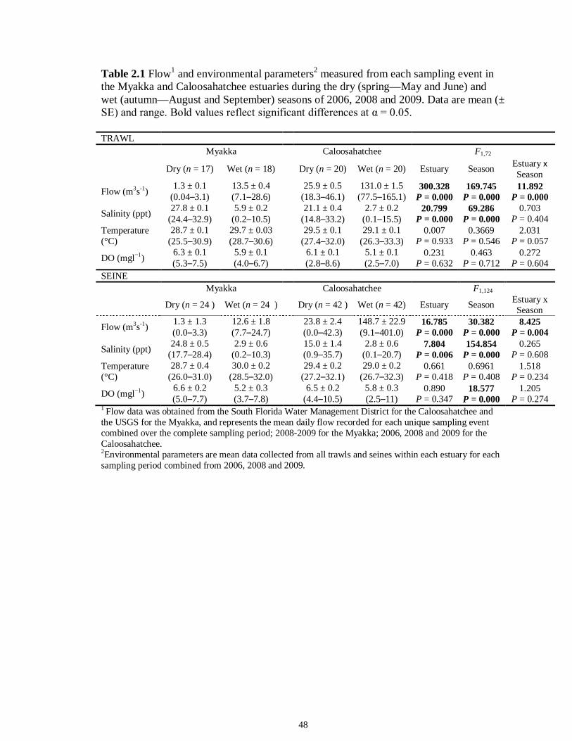
48

Table 2.1 Flow1 and environmental parameters2 measured from each sampling event in the Myakka and Caloosahatchee estuaries during the dry (spring—May and June) and wet (autumn—August and September) seasons of 2006, 2008 and 2009. Data are mean (± SE) and range. Bold values reflect significant differences at α = 0.05.

1 Flow data was obtained from the South Florida Water Management District for the Caloosahatchee and the USGS for the Myakka, and represents the mean daily flow recorded for each unique sampling event combined over the complete sampling period; 2008-2009 for the Myakka; 2006, 2008 and 2009 for the Caloosahatchee. 2Environmental parameters are mean data collected from all trawls and seines within each estuary for each sampling period combined from 2006, 2008 and 2009.

TRAWL Myakka Caloosahatchee F1,72

Dry (n = 17) Wet (n = 18) Dry (n = 20) Wet (n = 20) Estuary Season Estuary x Season

Flow (m3s-1) 1.3 ± 0.1 (0.04–3.1)

13.5 ± 0.4 (7.1–28.6) 25.9 ± 0.5

(18.3–46.1) 131.0 ± 1.5

(77.5–165.1) 300.328

P = 0.000 169.745

P = 0.000 11.892

P = 0.000

Salinity (ppt) 27.8 ± 0.1 (24.4–32.9)

5.9 ± 0.2 (0.2–10.5) 21.1 ± 0.4

(14.8–33.2) 2.7 ± 0.2

(0.1–15.5) 20.799

P = 0.000 69.286

P = 0.000 0.703

P = 0.404 Temperature (°C)

28.7 ± 0.1 (25.5–30.9)

29.7 ± 0.03 (28.7–30.6) 29.5 ± 0.1

(27.4–32.0) 29.1 ± 0.1

(26.3–33.3) 0.007

P = 0.933 0.3669

P = 0.546 2.031

P = 0.057

DO (mgl−1) 6.3 ± 0.1 (5.3–7.5)

5.9 ± 0.1 (4.0–6.7) 6.1 ± 0.1

(2.8–8.6) 5.1 ± 0.1 (2.5–7.0)

0.231 P = 0.632

0.463 P = 0.712

0.272 P = 0.604

SEINE Myakka Caloosahatchee F1,124

Dry (n = 24 ) Wet (n = 24 ) Dry (n = 42 ) Wet (n = 42) Estuary Season Estuary x Season

Flow (m3s-1) 1.3 ± 1.3 (0.0–3.3)

12.6 ± 1.8 (7.7–24.7) 23.8 ± 2.4

(0.0–42.3) 148.7 ± 22.9 (9.1–401.0)

16.785 P = 0.000

30.382 P = 0.000

8.425 P = 0.004

Salinity (ppt) 24.8 ± 0.5 (17.7–28.4)

2.9 ± 0.6 (0.2–10.3) 15.0 ± 1.4

(0.9–35.7) 2.8 ± 0.6

(0.1–20.7) 7.804

P = 0.006 154.854

P = 0.000 0.265

P = 0.608 Temperature (°C)

28.7 ± 0.4 (26.0–31.0)

30.0 ± 0.2 (28.5–32.0) 29.4 ± 0.2

(27.2–32.1) 29.0 ± 0.2

(26.7–32.3) 0.661

P = 0.418 0.6961

P = 0.408 1.518

P = 0.234

DO (mgl−1) 6.6 ± 0.2 (5.0–7.7)

5.2 ± 0.3 (3.7–7.8) 6.5 ± 0.2

(4.4–10.5) 5.8 ± 0.3 (2.5–11)

0.890 P = 0.347

18.577 P = 0.000

1.205 P = 0.274

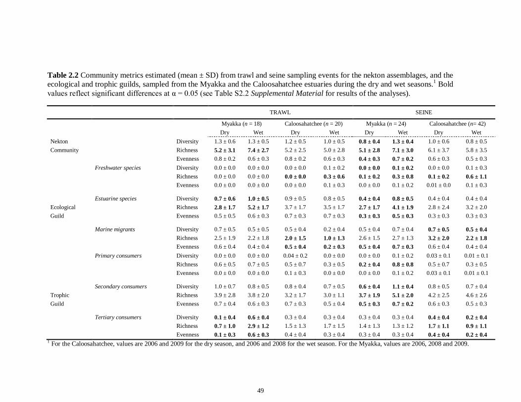
49

Table 2.2 Community metrics estimated (mean ± SD) from trawl and seine sampling events for the nekton assemblages, and the ecological and trophic guilds, sampled from the Myakka and the Caloosahatchee estuaries during the dry and wet seasons.1 Bold values reflect significant differences at α = 0.05 (see Table S2.2 Supplemental Material for results of the analyses).

TRAWL SEINE

Myakka (n = 18) Caloosahatchee (n = 20) Myakka (n = 24) Caloosahatchee (n= 42) Dry Wet Dry Wet Dry Wet Dry Wet Nekton Diversity 1.3 ± 0.6 1.3 ± 0.5 1.2 ± 0.5 1.0 ± 0.5 0.8 ± 0.4 1.3 ± 0.4 1.0 ± 0.6 0.8 ± 0.5 Community Richness 5.2 ± 3.1 7.4 ± 2.7 5.2 ± 2.5 5.0 ± 2.8 5.1 ± 2.8 7.1 ± 3.0 6.1 ± 3.7 5.8 ± 3.5 Evenness 0.8 ± 0.2 0.6 ± 0.3 0.8 ± 0.2 0.6 ± 0.3 0.4 ± 0.3 0.7 ± 0.2 0.6 ± 0.3 0.5 ± 0.3 Freshwater species Diversity 0.0 ± 0.0 0.0 ± 0.0 0.0 ± 0.0 0.1 ± 0.2 0.0 ± 0.0 0.1 ± 0.2 0.0 ± 0.0 0.1 ± 0.3 Richness 0.0 ± 0.0 0.0 ± 0.0 0.0 ± 0.0 0.3 ± 0.6 0.1 ± 0.2 0.3 ± 0.8 0.1 ± 0.2 0.6 ± 1.1 Evenness 0.0 ± 0.0 0.0 ± 0.0 0.0 ± 0.0 0.1 ± 0.3 0.0 ± 0.0 0.1 ± 0.2 0.01 ± 0.0 0.1 ± 0.3 Estuarine species Diversity 0.7 ± 0.6 1.0 ± 0.5 0.9 ± 0.5 0.8 ± 0.5 0.4 ± 0.4 0.8 ± 0.5 0.4 ± 0.4 0.4 ± 0.4 Ecological Richness 2.8 ± 1.7 5.2 ± 1.7 3.7 ± 1.7 3.5 ± 1.7 2.7 ± 1.7 4.1 ± 1.9 2.8 ± 2.4 3.2 ± 2.0 Guild Evenness 0.5 ± 0.5 0.6 ± 0.3 0.7 ± 0.3 0.7 ± 0.3 0.3 ± 0.3 0.5 ± 0.3 0.3 ± 0.3 0.3 ± 0.3 Marine migrants Diversity 0.7 ± 0.5 0.5 ± 0.5 0.5 ± 0.4 0.2 ± 0.4 0.5 ± 0.4 0.7 ± 0.4 0.7 ± 0.5 0.5 ± 0.4 Richness 2.5 ± 1.9 2.2 ± 1.8 2.0 ± 1.5 1.0 ± 1.3 2.6 ± 1.5 2.7 ± 1.3 3.2 ± 2.0 2.2 ± 1.8 Evenness 0.6 ± 0.4 0.4 ± 0.4 0.5 ± 0.4 0.2 ± 0.3 0.5 ± 0.4 0.7 ± 0.3 0.6 ± 0.4 0.4 ± 0.4 Primary consumers Diversity 0.0 ± 0.0 0.0 ± 0.0 0.04 ± 0.2 0.0 ± 0.0 0.0 ± 0.0 0.1 ± 0.2 0.03 ± 0.1 0.01 ± 0.1 Richness 0.6 ± 0.5 0.7 ± 0.5 0.5 ± 0.7 0.3 ± 0.5 0.2 ± 0.4 0.8 ± 0.8 0.5 ± 0.7 0.3 ± 0.5 Evenness 0.0 ± 0.0 0.0 ± 0.0 0.1 ± 0.3 0.0 ± 0.0 0.0 ± 0.0 0.1 ± 0.2 0.03 ± 0.1 0.01 ± 0.1 Secondary consumers Diversity 1.0 ± 0.7 0.8 ± 0.5 0.8 ± 0.4 0.7 ± 0.5 0.6 ± 0.4 1.1 ± 0.4 0.8 ± 0.5 0.7 ± 0.4 Trophic Richness 3.9 ± 2.8 3.8 ± 2.0 3.2 ± 1.7 3.0 ± 1.1 3.7 ± 1.9 5.1 ± 2.0 4.2 ± 2.5 4.6 ± 2.6 Guild Evenness 0.7 ± 0.4 0.6 ± 0.3 0.7 ± 0.3 0.5 ± 0.4 0.5 ± 0.3 0.7 ± 0.2 0.6 ± 0.3 0.5 ± 0.3 Tertiary consumers Diversity 0.1 ± 0.4 0.6 ± 0.4 0.3 ± 0.4 0.3 ± 0.4 0.3 ± 0.4 0.3 ± 0.4 0.4 ± 0.4 0.2 ± 0.4 Richness 0.7 ± 1.0 2.9 ± 1.2 1.5 ± 1.3 1.7 ± 1.5 1.4 ± 1.3 1.3 ± 1.2 1.7 ± 1.1 0.9 ± 1.1 Evenness 0.1 ± 0.3 0.6 ± 0.3 0.4 ± 0.4 0.3 ± 0.4 0.3 ± 0.4 0.3 ± 0.4 0.4 ± 0.4 0.2 ± 0.4

1 For the Caloosahatchee, values are 2006 and 2009 for the dry season, and 2006 and 2008 for the wet season. For the Myakka, values are 2006, 2008 and 2009.

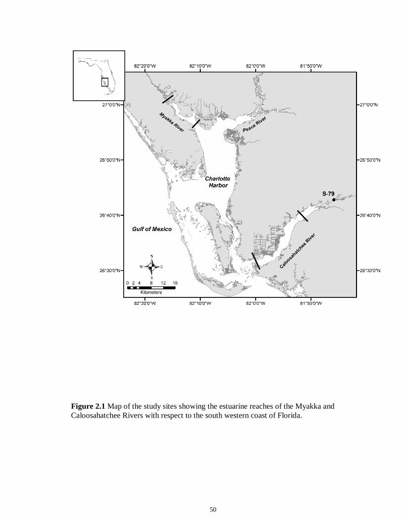
50

Figure 2.1 Map of the study sites showing the estuarine reaches of the Myakka and Caloosahatchee Rivers with respect to the south western coast of Florida.

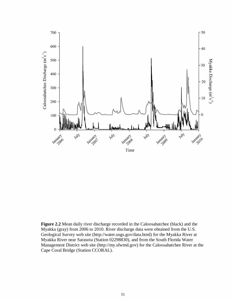
51

Figure 2.2 Mean daily river discharge recorded in the Caloosahatchee (black) and the Myakka (gray) from 2006 to 2010. River discharge data were obtained from the U.S. Geological Survey web site (http://water.usgs.gov/data.html) for the Myakka River at Myakka River near Sarasota (Station 02298830), and from the South Florida Water Management District web site (http://my.sfwmd.gov) for the Caloosahatchee River at the Cape Coral Bridge (Station CCORAL).

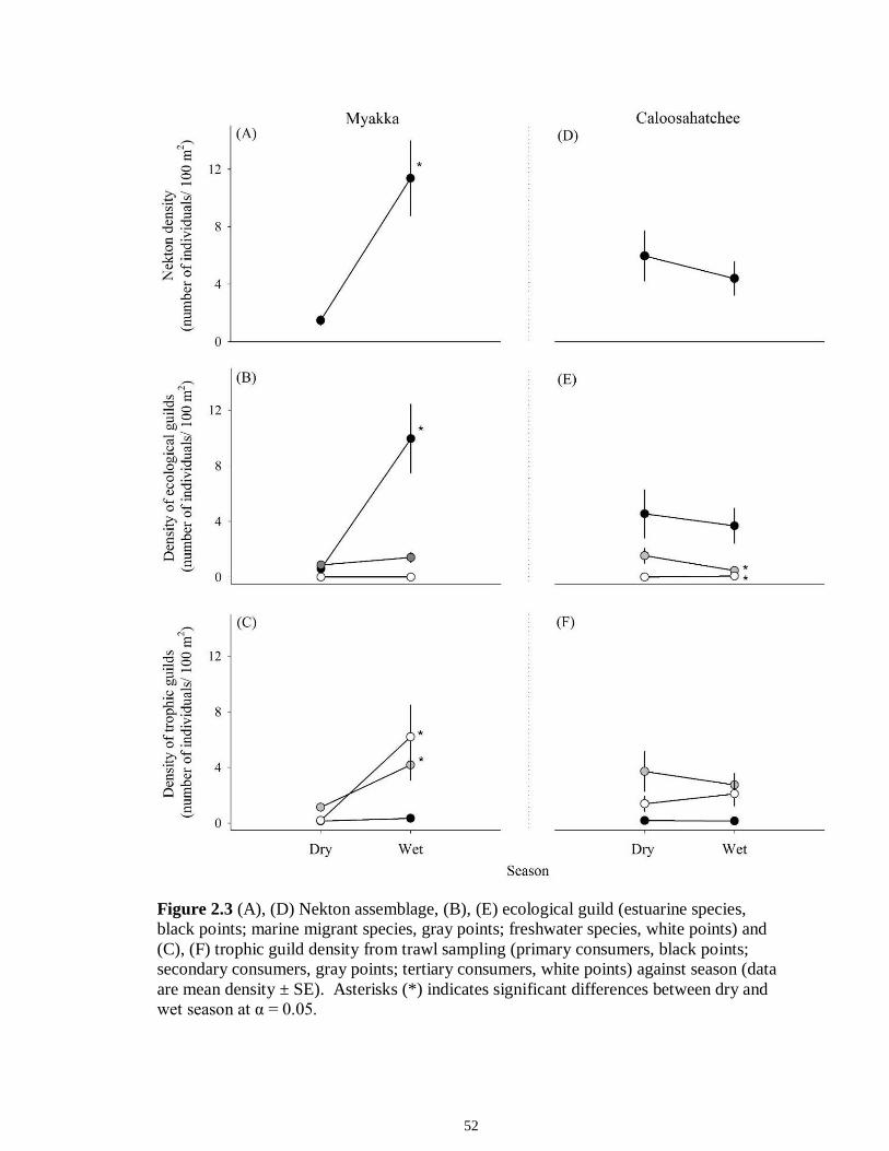
52

Figure 2.3 (A), (D) Nekton assemblage, (B), (E) ecological guild (estuarine species, black points; marine migrant species, gray points; freshwater species, white points) and (C), (F) trophic guild density from trawl sampling (primary consumers, black points; secondary consumers, gray points; tertiary consumers, white points) against season (data are mean density ± SE). Asterisks (*) indicates significant differences between dry and wet season at α = 0.05.

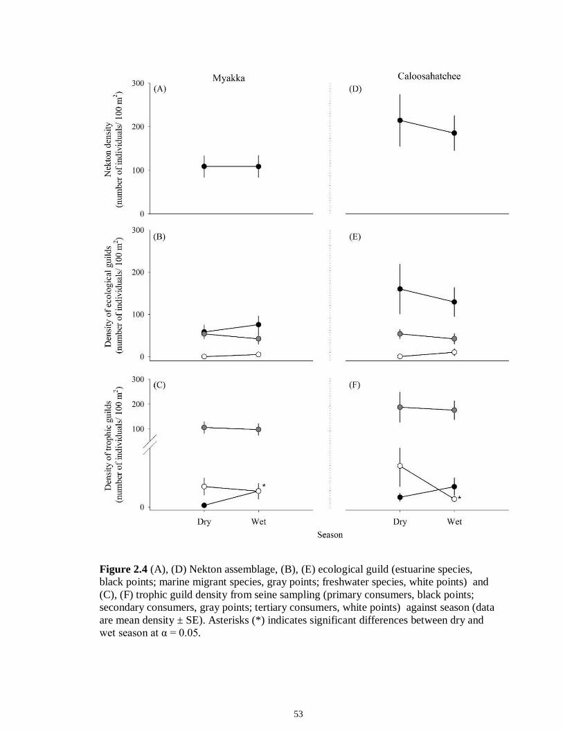
53

Figure 2.4 (A), (D) Nekton assemblage, (B), (E) ecological guild (estuarine species, black points; marine migrant species, gray points; freshwater species, white points) and (C), (F) trophic guild density from seine sampling (primary consumers, black points; secondary consumers, gray points; tertiary consumers, white points) against season (data are mean density ± SE). Asterisks (*) indicates significant differences between dry and wet season at α = 0.05.

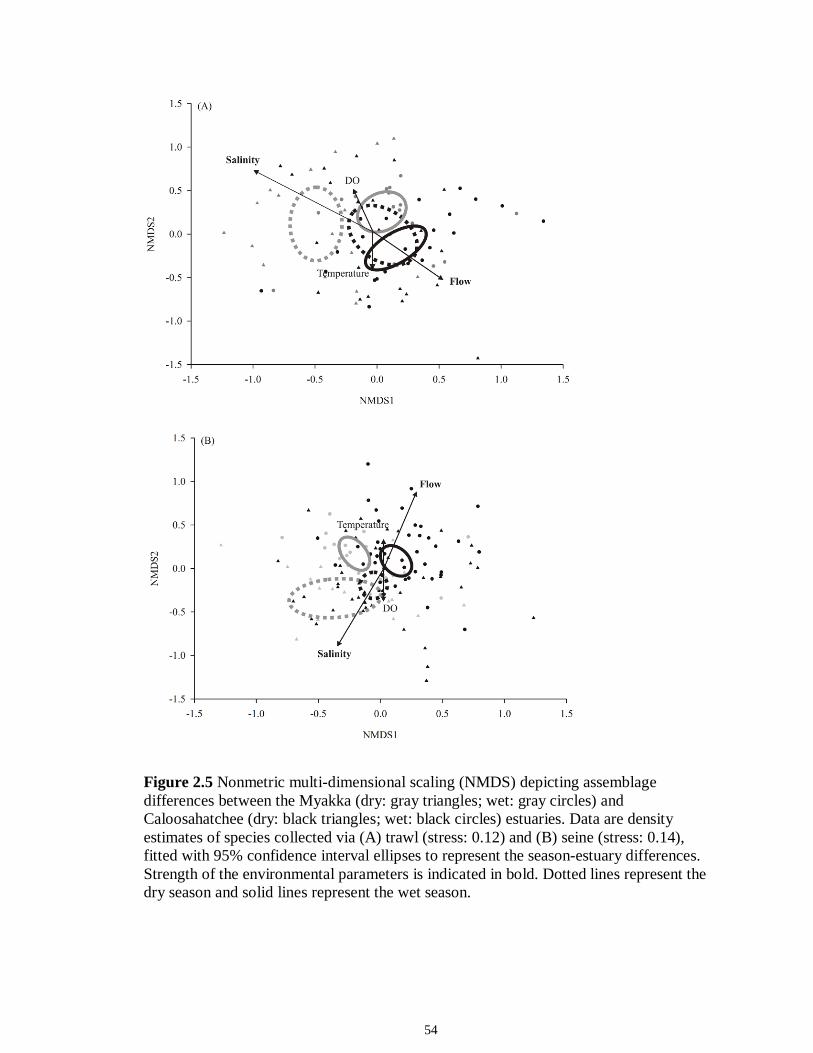
54

Figure 2.5 Nonmetric multi-dimensional scaling (NMDS) depicting assemblage differences between the Myakka (dry: gray triangles; wet: gray circles) and Caloosahatchee (dry: black triangles; wet: black circles) estuaries. Data are density estimates of species collected via (A) trawl (stress: 0.12) and (B) seine (stress: 0.14), fitted with 95% confidence interval ellipses to represent the season-estuary differences. Strength of the environmental parameters is indicated in bold. Dotted lines represent the dry season and solid lines represent the wet season.

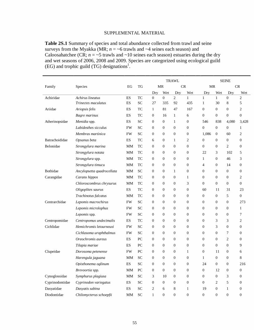
55

SUPPLEMENTAL MATERIAL Table 2S.1 Summary of species and total abundance collected from trawl and seine surveys from the Myakka (MR; n = ~6 trawls and ~4 seines each season) and Caloosahatchee (CR; n = ~5 trawls and ~10 seines each season) estuaries during the dry and wet seasons of 2006, 2008 and 2009. Species are categorized using ecological guild (EG) and trophic guild (TG) designations1.

TRAWL

SEINE Family Species EG TG MR CR MR CR

Dry Wet Dry Wet Dry Wet Dry Wet Achiridae Achirus lineatus ES TC 0 0 2 1 1 1 0 2 Trinectes maculatus ES SC 27 335 92 435 1 30 8 5 Ariidae Ariopsis felis ES TC 1 81 47 167 0 0 0 2 Bagre marinus ES TC 0 16 1 6 0 0 0 0 Atherinopsidae Menidia spp. ES SC 0 0 1 0 546 838 4,080 3,428 Labidesthes sicculus FW SC 0 0 0 0 0 0 0 1 Membras martinica FW SC 0 0 0 0 1,086 0 60 2 Batrachoididae Opsanus beta ES TC 6 0 1 2 0 0 0 0 Belonidae Strongylura marina MM TC 0 0 0 0 0 0 2 0 Strongylura notata MM TC 0 0 0 0 22 3 102 5 Strongylura spp. MM TC 0 0 0 0 1 0 46 3 Strongylura timucu MM TC 0 0 0 0 4 0 14 0 Bothidae Ancylopsetta quadrocellata MM SC 0 0 1 0 0 0 0 0 Carangidae Caranx hippos MM TC 0 0 0 1 0 0 0 2 Chloroscombrus chrysurus MM TC 0 0 0 3 0 0 0 0 Oligoplites saurus ES TC 0 0 0 0 60 11 31 23 Trachinotus falcatus MM TC 0 0 0 0 0 0 5 0 Centrarchidae Lepomis macrochirus FW SC 0 0 0 0 0 0 0 273 Lepomis microlophus FW SC 0 0 0 0 0 0 0 1 Lepomis spp. FW SC 0 0 0 0 0 0 0 7 Centropomidae Centropomus undecimalis ES TC 0 0 0 0 0 3 3 2 Cichlidae Hemichromis letourneuxi FW SC 0 0 0 0 0 3 0 0 Cichlasoma urophthalmus FW SC 0 0 0 0 0 0 7 0 Oreochromis aureus ES PC 0 0 0 0 0 0 2 0 Tilapia mariae ES PC 0 0 0 0 0 0 0 9 Clupeidae Dorosoma petenense FW PC 0 0 0 1 0 11 0 6 Harengula jaguana MM SC 0 0 0 0 1 0 0 8 Opisthonema oglinum ES SC 0 0 0 0 24 0 0 216 Brevoortia spp. MM PC 0 0 0 0 0 12 0 0 Cynoglossidae Symphurus plagiusa MM SC 3 10 0 0 0 0 3 0 Cyprinodontidae Cyprinodon variegatus ES SC 0 0 0 0 0 2 5 0 Dasyatidae Dasyatis sabina ES SC 2 6 8 1 19 0 1 0 Diodontidae Chilomycterus schoepfii MM SC 1 0 0 0 0 0 0 0

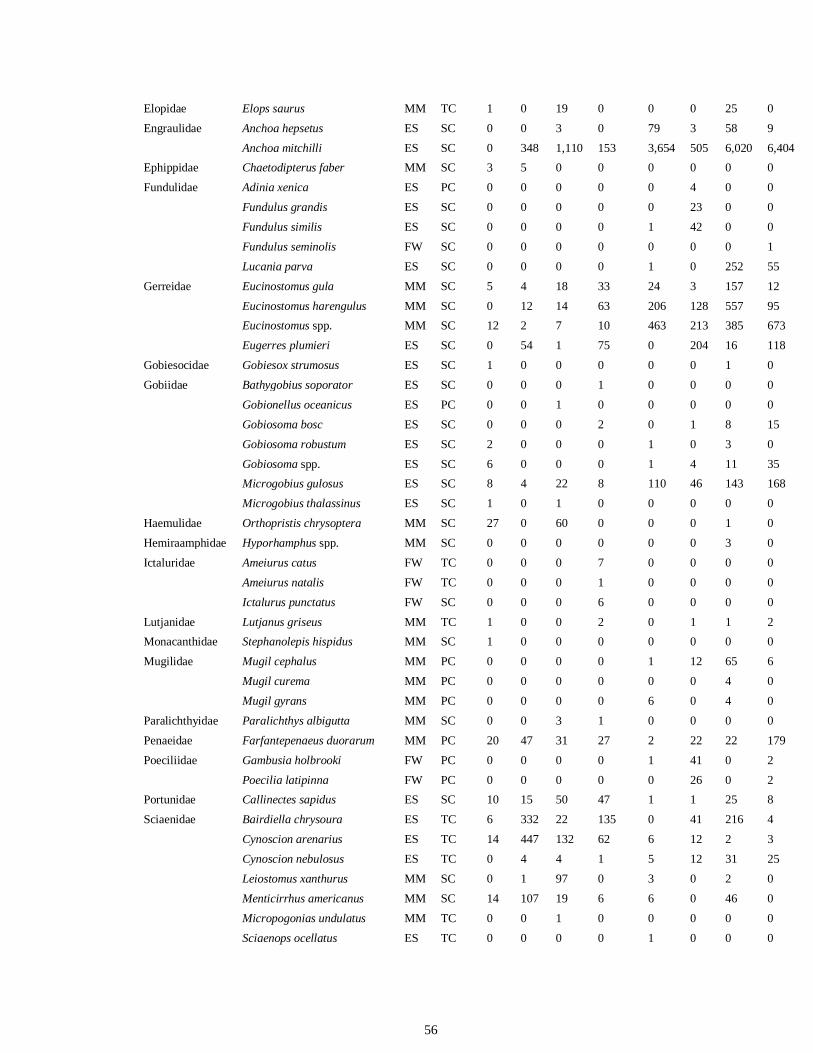
56

Elopidae Elops saurus MM TC 1 0 19 0 0 0 25 0 Engraulidae Anchoa hepsetus ES SC 0 0 3 0 79 3 58 9 Anchoa mitchilli ES SC 0 348 1,110 153 3,654 505 6,020 6,404 Ephippidae Chaetodipterus faber MM SC 3 5 0 0 0 0 0 0 Fundulidae Adinia xenica ES PC 0 0 0 0 0 4 0 0 Fundulus grandis ES SC 0 0 0 0 0 23 0 0 Fundulus similis ES SC 0 0 0 0 1 42 0 0 Fundulus seminolis FW SC 0 0 0 0 0 0 0 1 Lucania parva ES SC 0 0 0 0 1 0 252 55 Gerreidae Eucinostomus gula MM SC 5 4 18 33 24 3 157 12 Eucinostomus harengulus MM SC 0 12 14 63 206 128 557 95 Eucinostomus spp. MM SC 12 2 7 10 463 213 385 673 Eugerres plumieri ES SC 0 54 1 75 0 204 16 118 Gobiesocidae Gobiesox strumosus ES SC 1 0 0 0 0 0 1 0 Gobiidae Bathygobius soporator ES SC 0 0 0 1 0 0 0 0 Gobionellus oceanicus ES PC 0 0 1 0 0 0 0 0 Gobiosoma bosc ES SC 0 0 0 2 0 1 8 15 Gobiosoma robustum ES SC 2 0 0 0 1 0 3 0 Gobiosoma spp. ES SC 6 0 0 0 1 4 11 35 Microgobius gulosus ES SC 8 4 22 8 110 46 143 168 Microgobius thalassinus ES SC 1 0 1 0 0 0 0 0 Haemulidae Orthopristis chrysoptera MM SC 27 0 60 0 0 0 1 0 Hemiraamphidae Hyporhamphus spp. MM SC 0 0 0 0 0 0 3 0 Ictaluridae Ameiurus catus FW TC 0 0 0 7 0 0 0 0 Ameiurus natalis FW TC 0 0 0 1 0 0 0 0 Ictalurus punctatus FW SC 0 0 0 6 0 0 0 0 Lutjanidae Lutjanus griseus MM TC 1 0 0 2 0 1 1 2 Monacanthidae Stephanolepis hispidus MM SC 1 0 0 0 0 0 0 0 Mugilidae Mugil cephalus MM PC 0 0 0 0 1 12 65 6 Mugil curema MM PC 0 0 0 0 0 0 4 0 Mugil gyrans MM PC 0 0 0 0 6 0 4 0 Paralichthyidae Paralichthys albigutta MM SC 0 0 3 1 0 0 0 0 Penaeidae Farfantepenaeus duorarum MM PC 20 47 31 27 2 22 22 179 Poeciliidae Gambusia holbrooki FW PC 0 0 0 0 1 41 0 2 Poecilia latipinna FW PC 0 0 0 0 0 26 0 2 Portunidae Callinectes sapidus ES SC 10 15 50 47 1 1 25 8 Sciaenidae Bairdiella chrysoura ES TC 6 332 22 135 0 41 216 4 Cynoscion arenarius ES TC 14 447 132 62 6 12 2 3 Cynoscion nebulosus ES TC 0 4 4 1 5 12 31 25 Leiostomus xanthurus MM SC 0 1 97 0 3 0 2 0 Menticirrhus americanus MM SC 14 107 19 6 6 0 46 0 Micropogonias undulatus MM TC 0 0 1 0 0 0 0 0 Sciaenops ocellatus ES TC 0 0 0 0 1 0 0 0

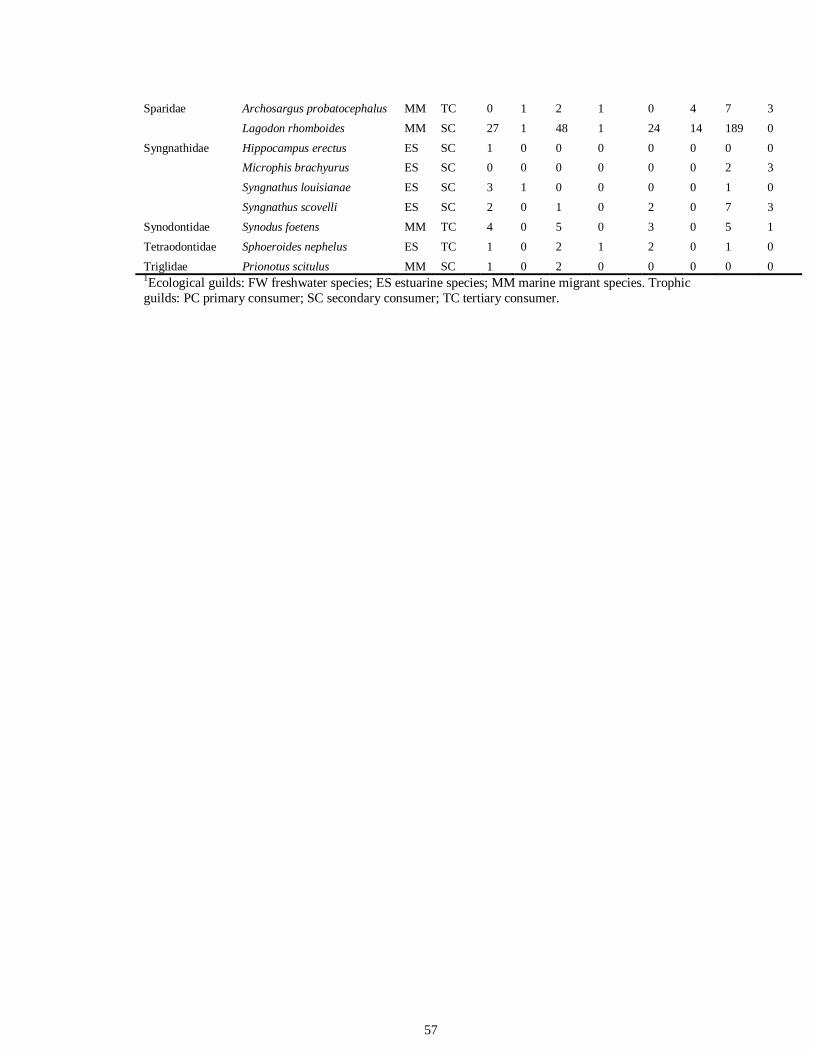
57

Sparidae Archosargus probatocephalus MM TC 0 1 2 1 0 4 7 3 Lagodon rhomboides MM SC 27 1 48 1 24 14 189 0 Syngnathidae Hippocampus erectus ES SC 1 0 0 0 0 0 0 0 Microphis brachyurus ES SC 0 0 0 0 0 0 2 3 Syngnathus louisianae ES SC 3 1 0 0 0 0 1 0 Syngnathus scovelli ES SC 2 0 1 0 2 0 7 3 Synodontidae Synodus foetens MM TC 4 0 5 0 3 0 5 1 Tetraodontidae Sphoeroides nephelus ES TC 1 0 2 1 2 0 1 0 Triglidae Prionotus scitulus MM SC 1 0 2 0 0 0 0 0 1Ecological guilds: FW freshwater species; ES estuarine species; MM marine migrant species. Trophic guilds: PC primary consumer; SC secondary consumer; TC tertiary consumer.

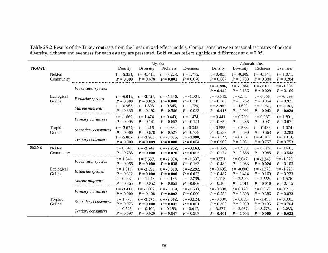
58

Table 2S.2 Results of the Tukey contrasts from the linear mixed-effect models. Comparisons between seasonal estimates of nekton diversity, richness and evenness for each estuary are presented. Bold values reflect significant differences at α = 0.05.

Myakka Caloosahatchee TRAWL Density Diversity Richness Evenness Density Diversity Richness Evenness Nekton

Community t = -5.354, P = 0.000

t = -0.415, P = 0.678

t = -3.223, P = 0.001

t = 1.775, P = 0.076

t = 0.403, P = 0.687

t = -0.309, P = 0.758

t = -0.146, P = 0.884

t = 1.071, P = 0.284

Freshwater species

t = -1.996, P = 0.046

t = -1.384, P = 0.166

t = -2.186, P = 0.029

t = -1.384, P = 0.166

Ecological Guilds Estuarine species t = -6.016,

P = 0.000 t = -2.423, P = 0.015

t = -5.336, P = 0.000

t = -1.004, P = 0.315

t = -0.545, P = 0.586

t = 0.343, P = 0.732

t = 0.058, P = 0.954

t = -0.099, P = 0.921

Marine migrants t = -0.963, P = 0.336

t = 1.303, P = 0.192

t = 0.545, P = 0.586

t = 1.729, P = 0.083

t = 2.360, P = 0.018

t = 1.692, P = 0.091

t = 2.037, P = 0.042

t = 2.181, P = 0.029

Primary consumers t = -1.669,

P = 0.095 t = 1.474, P = 0.141

t = 0.449, P = 0.653

t = 1.474, P = 0.141

t = 0.441, P = 0.659

t = 0.780, P = 0.435

t = 0.087, P = 0.931

t = 1.801, P = 0.071

Trophic Guilds Secondary consumers t = -3.629,

P = 0.000 t = 0.416, P = 0.678

t = -0.632, P = 0.527

t = 0.345, P = 0.738

t = 0.585, P = 0.559

t = 0.538, P = 0.590

t = -0.436, P = 0.663

t = 1.074, P = 0.283

Tertiary consumers t = -5.007, P = 0.000

t = -3.900, P = 0.009

t = -5.635, P = 0.000

t = -4.098, P = 0.004

t = -0.122, P = 0.903

t = 0.087, P = 0.931

t = -0.309, P = 0.757

t = 0.314, P = 0.753

SEINE Nekton Community t = 0.341,

P = 0.733 t = -3.747, P = 0.000

t = -2.232, P = 0.026

t = -3.163, P = 0.002 t = -1.359,

P = 0.174 t = 0.905, P = 0.366

t = 0.018, P = 0.985

t = 0.601, P = 0.548

Freshwater species t = 1.841,

P = 0.066 t = 3.537, P = 0.000

t = -2.074, P = 0.038

t = -1.397, P = 0.163

t = 0.551, P = 0.480

t = 0.047, P = 0.063

t = -2.246, P = 0.024

t = -1.629, P = 0.103

Ecological Guilds Estuarine species t = 1.011,

P = 0.312 t = -3.690, P = 0.000

t = -3.318, P = 0.000

t = -2.292, P = 0.022

t = -0.695, P = 0.487

t = -0.800, P = 0.424

t = -1.375, P = 0.169

t = -1.220, P = 0.223

Marine migrants t = 0.907, P = 0.365

t = -1.943, P = 0.052

t = -0.185, P = 0.853

t = -2.739, P = 0.006

t = 1.115, P = 0.265

t = 2.520, P = 0.011

t = 2.559, P = 0.010

t = 1.576, P = 0.115

Primary consumers t = -3.419,

P = 0.000 t = -1.607, P = 0.108

t = -3.079, P = 0.002

t = -1.693, P = 0.090

t = -0.598, P = 0.550

t = 0.128, P = 0.898

t = 0.867, P = 0.386

t = 0.211, P = 0.833

Trophic Guilds Secondary consumers t = 1.779,

P = 0.075 t = -3.575, P = 0.000

t = -2.082, P = 0.037

t = -3.124, P = 0.001

t = -0.900, P = 0.368

t = 0.089, P = 0.929

t = -1.495, P = 0.135

t = 0.381, P = 0.704

Tertiary consumers t = 0.529, P = 0.597

t = -0.100, P = 0.920

t = 0.193, P = 0.847

t = 0.017, P = 0.987

t = 3.277, P = 0.001

t = 2.957, P = 0.003

t = 3.775, P = 0.000

t = 2.233, P = 0.025

59

CHAPTER 3

MATERNAL MEDDLING IN NEONATAL SHARKS: IMPLICATIONS FOR

INTERPRETING STABLE ISOTOPES IN YOUNG ANIMALS*

* Olin JA, Hussey NE, Fritts M, Heupel MR, Simpfendorfer CA, Poulakis GR, Fisk AT. 2011. Maternal meddling in neonatal sharks: implications for interpreting stable isotopes in young animals. Rapid Communications in Mass Spectrometry 25:1008-1016.

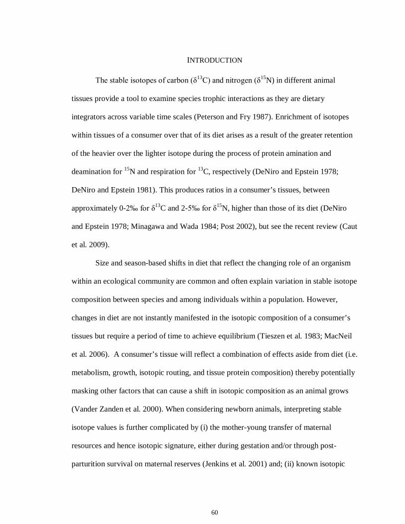
60

INTRODUCTION

The stable isotopes of carbon (δ13C) and nitrogen (δ15N) in different animal

tissues provide a tool to examine species trophic interactions as they are dietary

integrators across variable time scales (Peterson and Fry 1987). Enrichment of isotopes

within tissues of a consumer over that of its diet arises as a result of the greater retention

of the heavier over the lighter isotope during the process of protein amination and

deamination for 15N and respiration for 13C, respectively (DeNiro and Epstein 1978;

DeNiro and Epstein 1981). This produces ratios in a consumer’s tissues, between

approximately 0-2‰ for δ13C and 2-5‰ for δ15N, higher than those of its diet (DeNiro

and Epstein 1978; Minagawa and Wada 1984; Post 2002), but see the recent review (Caut

et al. 2009).

Size and season-based shifts in diet that reflect the changing role of an organism

within an ecological community are common and often explain variation in stable isotope

composition between species and among individuals within a population. However,

changes in diet are not instantly manifested in the isotopic composition of a consumer’s

tissues but require a period of time to achieve equilibrium (Tieszen et al. 1983; MacNeil

et al. 2006). A consumer’s tissue will reflect a combination of effects aside from diet (i.e.

metabolism, growth, isotopic routing, and tissue protein composition) thereby potentially

masking other factors that can cause a shift in isotopic composition as an animal grows

(Vander Zanden et al. 2000). When considering newborn animals, interpreting stable

isotope values is further complicated by (i) the mother-young transfer of maternal

resources and hence isotopic signature, either during gestation and/or through post-

parturition survival on maternal reserves (Jenkins et al. 2001) and; (ii) known isotopic

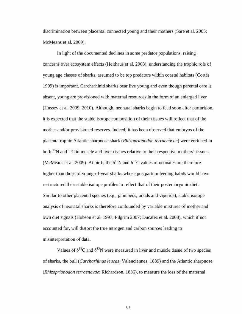
61

discrimination between placental connected young and their mothers (Sare et al. 2005;

McMeans et al. 2009).

In light of the documented declines in some predator populations, raising

concerns over ecosystem effects (Heithaus et al. 2008), understanding the trophic role of

young age classes of sharks, assumed to be top predators within coastal habitats (Cortés

1999) is important. Carcharhinid sharks bear live young and even though parental care is

absent, young are provisioned with maternal resources in the form of an enlarged liver

(Hussey et al. 2009, 2010). Although, neonatal sharks begin to feed soon after parturition,

it is expected that the stable isotope composition of their tissues will reflect that of the

mother and/or provisioned reserves. Indeed, it has been observed that embryos of the

placentatrophic Atlantic sharpnose shark (Rhizoprionodon terraenovae) were enriched in

both 15N and 13C in muscle and liver tissues relative to their respective mothers’ tissues

(McMeans et al. 2009). At birth, the δ15N and δ13C values of neonates are therefore

higher than those of young-of-year sharks whose postpartum feeding habits would have

restructured their stable isotope profiles to reflect that of their postembryonic diet.

Similar to other placental species (e.g., pinnipeds, ursids and viperids), stable isotope

analysis of neonatal sharks is therefore confounded by variable mixtures of mother and

own diet signals (Hobson et al. 1997; Pilgrim 2007; Ducatez et al. 2008), which if not

accounted for, will distort the true nitrogen and carbon sources leading to

misinterpretation of data.

Values of δ13C and δ15N were measured in liver and muscle tissue of two species

of sharks, the bull (Carcharhinus leucas; Valenciennes, 1839) and the Atlantic sharpnose

(Rhizoprionodon terraenovae; Richardson, 1836), to measure the loss of the maternal

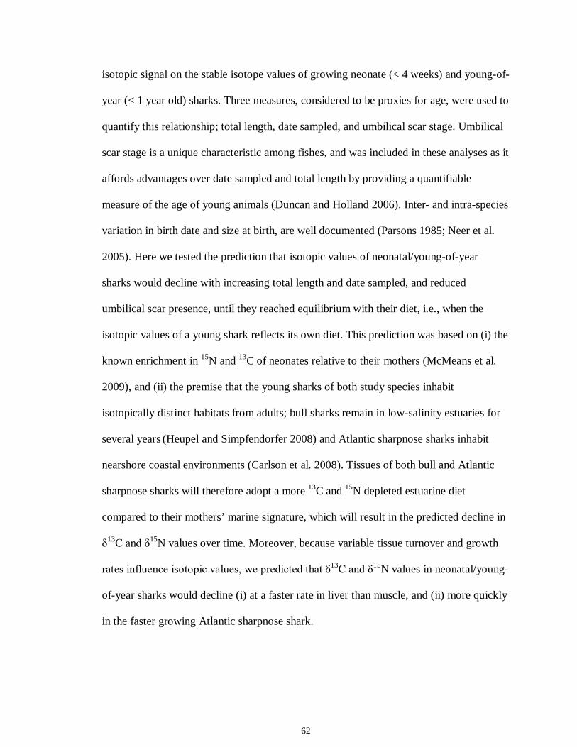
62

isotopic signal on the stable isotope values of growing neonate (< 4 weeks) and young-of-

year (< 1 year old) sharks. Three measures, considered to be proxies for age, were used to

quantify this relationship; total length, date sampled, and umbilical scar stage. Umbilical

scar stage is a unique characteristic among fishes, and was included in these analyses as it

affords advantages over date sampled and total length by providing a quantifiable

measure of the age of young animals (Duncan and Holland 2006). Inter- and intra-species

variation in birth date and size at birth, are well documented (Parsons 1985; Neer et al.

2005). Here we tested the prediction that isotopic values of neonatal/young-of-year

sharks would decline with increasing total length and date sampled, and reduced

umbilical scar presence, until they reached equilibrium with their diet, i.e., when the

isotopic values of a young shark reflects its own diet. This prediction was based on (i) the

known enrichment in 15N and 13C of neonates relative to their mothers (McMeans et al.

2009), and (ii) the premise that the young sharks of both study species inhabit

isotopically distinct habitats from adults; bull sharks remain in low-salinity estuaries for

several years (Heupel and Simpfendorfer 2008) and Atlantic sharpnose sharks inhabit

nearshore coastal environments (Carlson et al. 2008). Tissues of both bull and Atlantic

sharpnose sharks will therefore adopt a more 13C and 15N depleted estuarine diet

compared to their mothers’ marine signature, which will result in the predicted decline in

δ13C and δ15N values over time. Moreover, because variable tissue turnover and growth

rates influence isotopic values, we predicted that δ13C and δ15N values in neonatal/young-

of-year sharks would decline (i) at a faster rate in liver than muscle, and (ii) more quickly

in the faster growing Atlantic sharpnose shark.

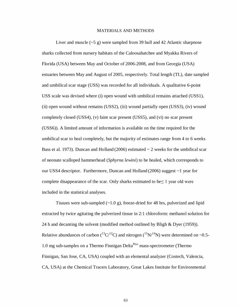
63

MATERIALS AND METHODS

Liver and muscle (~5 g) were sampled from 39 bull and 42 Atlantic sharpnose

sharks collected from nursery habitats of the Caloosahatchee and Myakka Rivers of

Florida (USA) between May and October of 2006-2008, and from Georgia (USA)

estuaries between May and August of 2005, respectively. Total length (TL), date sampled

and umbilical scar stage (USS) was recorded for all individuals. A qualitative 6-point

USS scale was devised where (i) open wound with umbilical remains attached (USS1),

(ii) open wound without remains (USS2), (iii) wound partially open (USS3), (iv) wound

completely closed (USS4), (v) faint scar present (USS5), and (vi) no scar present

(USS6)). A limited amount of information is available on the time required for the

umbilical scar to heal completely, but the majority of estimates range from 4 to 6 weeks

Bass et al. 1973). Duncan and Holland (2006) estimated ~ 2 weeks for the umbilical scar

of neonate scalloped hammerhead (Sphyrna lewini) to be healed, which corresponds to

our USS4 descriptor. Furthermore, Duncan and Holland (2006) suggest ~1 year for

complete disappearance of the scar. Only sharks estimated to be ≤ 1 year old were

included in the statistical analyses.

Tissues were sub-sampled (~1.0 g), freeze-dried for 48 hrs, pulverized and lipid

extracted by twice agitating the pulverized tissue in 2:1 chloroform: methanol solution for

24 h and decanting the solvent (modified method outlined by Bligh & Dyer (1959)).

Relative abundances of carbon (13C/12C) and nitrogen (15N/14N) were determined on ~0.5-

1.0 mg sub-samples on a Thermo Finnigan DeltaPlus mass-spectrometer (Thermo

Finnigan, San Jose, CA, USA) coupled with an elemental analyzer (Costech, Valencia,

CA, USA) at the Chemical Tracers Laboratory, Great Lakes Institute for Environmental

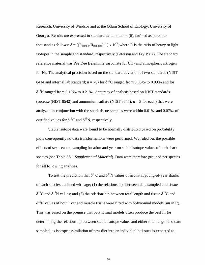
64

Research, University of Windsor and at the Odum School of Ecology, University of

Georgia. Results are expressed in standard delta notation (δ), defined as parts per

thousand as follows: δ = [(Rsample/Rstandard)-1] x 103, where R is the ratio of heavy to light

isotopes in the sample and standard, respectively (Peterson and Fry 1987). The standard

reference material was Pee Dee Belemnite carbonate for CO2 and atmospheric nitrogen

for N2. The analytical precision based on the standard deviation of two standards (NIST

8414 and internal lab standard; n = 76) for δ13C ranged from 0.06‰ to 0.09‰ and for

δ15N ranged from 0.10‰ to 0.21‰. Accuracy of analysis based on NIST standards

(sucrose (NIST 8542) and ammonium sulfate (NIST 8547); n = 3 for each) that were

analyzed in-conjunction with the shark tissue samples were within 0.01‰ and 0.07‰ of

certified values for δ13C and δ15N, respectively.

Stable isotope data were found to be normally distributed based on probability

plots consequently no data transformations were performed. We ruled out the possible

effects of sex, season, sampling location and year on stable isotope values of both shark

species (see Table 3S.1 Supplemental Material). Data were therefore grouped per species

for all following analyses.

To test the prediction that δ13C and δ15N values of neonatal/young-of-year sharks

of each species declined with age; (1) the relationships between date sampled and tissue

δ13C and δ15N values; and (2) the relationship between total length and tissue δ13C and

δ15N values of both liver and muscle tissue were fitted with polynomial models (lm in R).

This was based on the premise that polynomial models often produce the best fit for

determining the relationship between stable isotope values and either total length and date

sampled, as isotope assimilation of new diet into an individual’s tissues is expected to

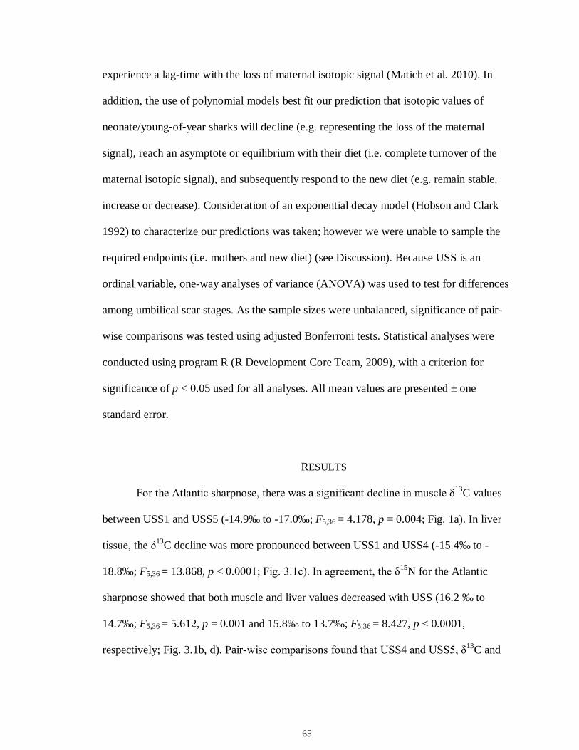
65

experience a lag-time with the loss of maternal isotopic signal (Matich et al. 2010). In

addition, the use of polynomial models best fit our prediction that isotopic values of

neonate/young-of-year sharks will decline (e.g. representing the loss of the maternal

signal), reach an asymptote or equilibrium with their diet (i.e. complete turnover of the

maternal isotopic signal), and subsequently respond to the new diet (e.g. remain stable,

increase or decrease). Consideration of an exponential decay model (Hobson and Clark

1992) to characterize our predictions was taken; however we were unable to sample the

required endpoints (i.e. mothers and new diet) (see Discussion). Because USS is an

ordinal variable, one-way analyses of variance (ANOVA) was used to test for differences

among umbilical scar stages. As the sample sizes were unbalanced, significance of pair-

wise comparisons was tested using adjusted Bonferroni tests. Statistical analyses were

conducted using program R (R Development Core Team, 2009), with a criterion for

significance of p < 0.05 used for all analyses. All mean values are presented ± one

standard error.

RESULTS

For the Atlantic sharpnose, there was a significant decline in muscle δ13C values

between USS1 and USS5 (-14.9‰ to -17.0‰; F5,36 = 4.178, p = 0.004; Fig. 1a). In liver

tissue, the δ13C decline was more pronounced between USS1 and USS4 (-15.4‰ to -

18.8‰; F5,36 = 13.868, p < 0.0001; Fig. 3.1c). In agreement, the δ15N for the Atlantic

sharpnose showed that both muscle and liver values decreased with USS (16.2 ‰ to

14.7‰; F5,36 = 5.612, p = 0.001 and 15.8‰ to 13.7‰; F5,36 = 8.427, p < 0.0001,

respectively; Fig. 3.1b, d). Pair-wise comparisons found that USS4 and USS5, δ13C and

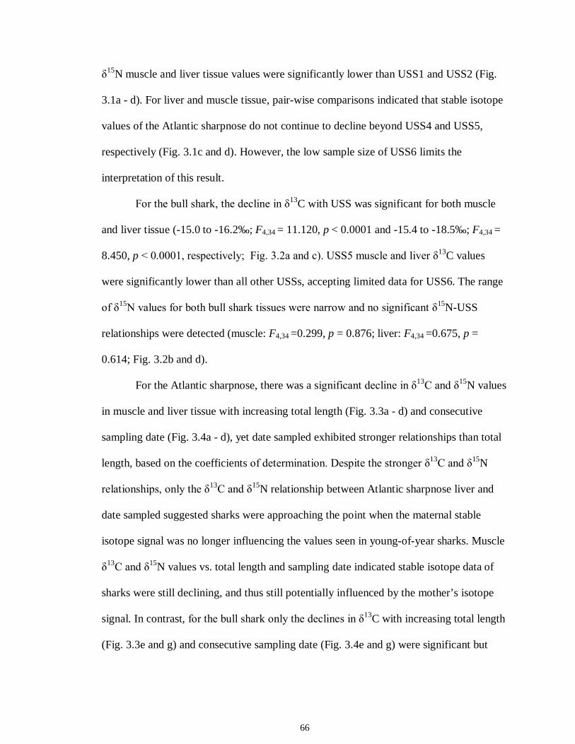
66

δ15N muscle and liver tissue values were significantly lower than USS1 and USS2 (Fig.

3.1a - d). For liver and muscle tissue, pair-wise comparisons indicated that stable isotope

values of the Atlantic sharpnose do not continue to decline beyond USS4 and USS5,

respectively (Fig. 3.1c and d). However, the low sample size of USS6 limits the

interpretation of this result.

For the bull shark, the decline in δ13C with USS was significant for both muscle

and liver tissue (-15.0 to -16.2‰; F4,34 = 11.120, p < 0.0001 and -15.4 to -18.5‰; F4,34 =

8.450, p < 0.0001, respectively; Fig. 3.2a and c). USS5 muscle and liver δ13C values

were significantly lower than all other USSs, accepting limited data for USS6. The range

of δ15N values for both bull shark tissues were narrow and no significant δ15N-USS

relationships were detected (muscle: F4,34 =0.299, p = 0.876; liver: F4,34 =0.675, p =

0.614; Fig. 3.2b and d).

For the Atlantic sharpnose, there was a significant decline in δ13C and δ15N values

in muscle and liver tissue with increasing total length (Fig. 3.3a - d) and consecutive

sampling date (Fig. 3.4a - d), yet date sampled exhibited stronger relationships than total

length, based on the coefficients of determination. Despite the stronger δ13C and δ15N

relationships, only the δ13C and δ15N relationship between Atlantic sharpnose liver and

date sampled suggested sharks were approaching the point when the maternal stable

isotope signal was no longer influencing the values seen in young-of-year sharks. Muscle

δ13C and δ15N values vs. total length and sampling date indicated stable isotope data of

sharks were still declining, and thus still potentially influenced by the mother’s isotope

signal. In contrast, for the bull shark only the declines in δ13C with increasing total length

(Fig. 3.3e and g) and consecutive sampling date (Fig. 3.4e and g) were significant but

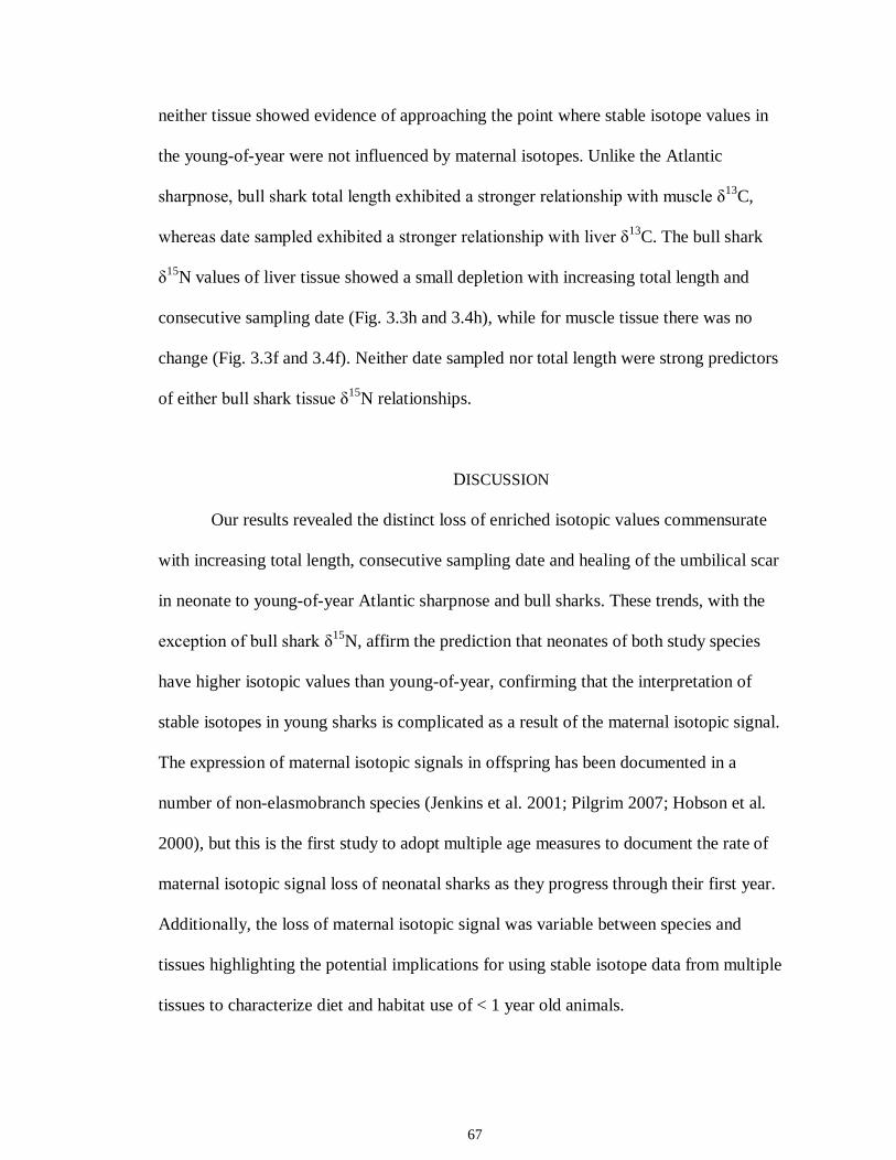
67

neither tissue showed evidence of approaching the point where stable isotope values in

the young-of-year were not influenced by maternal isotopes. Unlike the Atlantic

sharpnose, bull shark total length exhibited a stronger relationship with muscle δ13C,

whereas date sampled exhibited a stronger relationship with liver δ13C. The bull shark

δ15N values of liver tissue showed a small depletion with increasing total length and

consecutive sampling date (Fig. 3.3h and 3.4h), while for muscle tissue there was no

change (Fig. 3.3f and 3.4f). Neither date sampled nor total length were strong predictors

of either bull shark tissue δ15N relationships.

DISCUSSION

Our results revealed the distinct loss of enriched isotopic values commensurate

with increasing total length, consecutive sampling date and healing of the umbilical scar

in neonate to young-of-year Atlantic sharpnose and bull sharks. These trends, with the

exception of bull shark δ15N, affirm the prediction that neonates of both study species

have higher isotopic values than young-of-year, confirming that the interpretation of

stable isotopes in young sharks is complicated as a result of the maternal isotopic signal.

The expression of maternal isotopic signals in offspring has been documented in a

number of non-elasmobranch species (Jenkins et al. 2001; Pilgrim 2007; Hobson et al.

2000), but this is the first study to adopt multiple age measures to document the rate of

maternal isotopic signal loss of neonatal sharks as they progress through their first year.

Additionally, the loss of maternal isotopic signal was variable between species and

tissues highlighting the potential implications for using stable isotope data from multiple

tissues to characterize diet and habitat use of < 1 year old animals.

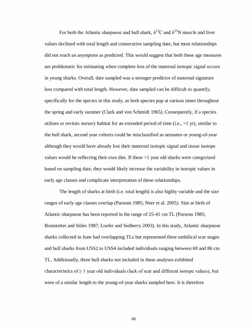
68

For both the Atlantic sharpnose and bull shark, δ13C and δ15N muscle and liver

values declined with total length and consecutive sampling date, but most relationships

did not reach an asymptote as predicted. This would suggest that both these age measures

are problematic for estimating when complete loss of the maternal isotopic signal occurs

in young sharks. Overall, date sampled was a stronger predictor of maternal signature

loss compared with total length. However, date sampled can be difficult to quantify,

specifically for the species in this study, as both species pup at various times throughout

the spring and early summer (Clark and von Schmidt 1965). Consequently, if a species

utilizes or revisits nursery habitat for an extended period of time (i.e., >1 yr), similar to

the bull shark, second year cohorts could be misclassified as neonates or young-of-year

although they would have already lost their maternal isotopic signal and tissue isotope

values would be reflecting their own diet. If these >1 year old sharks were categorized

based on sampling date, they would likely increase the variability in isotopic values in

early age classes and complicate interpretation of these relationships.

The length of sharks at birth (i.e. total length) is also highly variable and the size

ranges of early age classes overlap (Parsons 1985; Neer et al. 2005). Size at birth of

Atlantic sharpnose has been reported in the range of 25-41 cm TL (Parsons 1985;

Branstetter and Stiles 1987; Loefer and Sedberry 2003). In this study, Atlantic sharpnose

sharks collected in June had overlapping TLs but represented three umbilical scar stages

and bull sharks from USS2 to USS4 included individuals ranging between 69 and 86 cm

TL. Additionally, three bull sharks not included in these analyses exhibited

characteristics of ≥ 1 year old individuals (lack of scar and different isotope values), but

were of a similar length to the young-of-year sharks sampled here. It is therefore

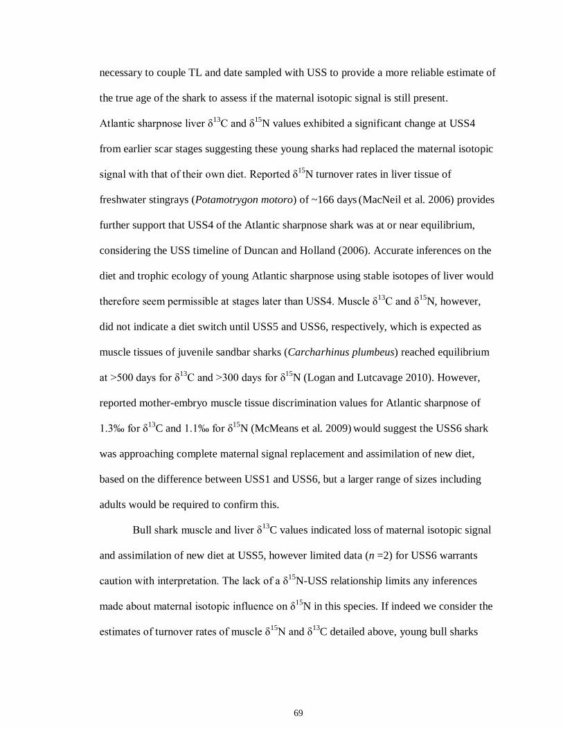
69

necessary to couple TL and date sampled with USS to provide a more reliable estimate of

the true age of the shark to assess if the maternal isotopic signal is still present.

Atlantic sharpnose liver δ13C and δ15N values exhibited a significant change at USS4

from earlier scar stages suggesting these young sharks had replaced the maternal isotopic

signal with that of their own diet. Reported δ15N turnover rates in liver tissue of

freshwater stingrays (Potamotrygon motoro) of ~166 days (MacNeil et al. 2006) provides

further support that USS4 of the Atlantic sharpnose shark was at or near equilibrium,

considering the USS timeline of Duncan and Holland (2006). Accurate inferences on the

diet and trophic ecology of young Atlantic sharpnose using stable isotopes of liver would

therefore seem permissible at stages later than USS4. Muscle δ13C and δ15N, however,

did not indicate a diet switch until USS5 and USS6, respectively, which is expected as

muscle tissues of juvenile sandbar sharks (Carcharhinus plumbeus) reached equilibrium

at >500 days for δ13C and >300 days for δ15N (Logan and Lutcavage 2010). However,

reported mother-embryo muscle tissue discrimination values for Atlantic sharpnose of

1.3‰ for δ13C and 1.1‰ for δ15N (McMeans et al. 2009) would suggest the USS6 shark

was approaching complete maternal signal replacement and assimilation of new diet,

based on the difference between USS1 and USS6, but a larger range of sizes including

adults would be required to confirm this.

Bull shark muscle and liver δ13C values indicated loss of maternal isotopic signal

and assimilation of new diet at USS5, however limited data (n =2) for USS6 warrants

caution with interpretation. The lack of a δ15N-USS relationship limits any inferences

made about maternal isotopic influence on δ15N in this species. If indeed we consider the

estimates of turnover rates of muscle δ15N and δ13C detailed above, young bull sharks

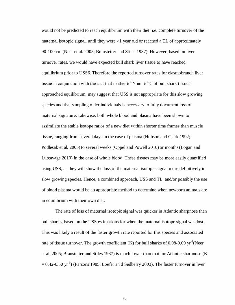
70

would not be predicted to reach equilibrium with their diet, i.e. complete turnover of the

maternal isotopic signal, until they were >1 year old or reached a TL of approximately

90-100 cm (Neer et al. 2005; Branstetter and Stiles 1987). However, based on liver

turnover rates, we would have expected bull shark liver tissue to have reached

equilibrium prior to USS6. Therefore the reported turnover rates for elasmobranch liver

tissue in conjunction with the fact that neither δ15N nor δ13C of bull shark tissues

approached equilibrium, may suggest that USS is not appropriate for this slow growing

species and that sampling older individuals is necessary to fully document loss of

maternal signature. Likewise, both whole blood and plasma have been shown to

assimilate the stable isotope ratios of a new diet within shorter time frames than muscle

tissue, ranging from several days in the case of plasma (Hobson and Clark 1992;

Podlesak et al. 2005) to several weeks (Oppel and Powell 2010) or months (Logan and

Lutcavage 2010) in the case of whole blood. These tissues may be more easily quantified

using USS, as they will show the loss of the maternal isotopic signal more definitively in

slow growing species. Hence, a combined approach, USS and TL, and/or possibly the use

of blood plasma would be an appropriate method to determine when newborn animals are

in equilibrium with their own diet.

The rate of loss of maternal isotopic signal was quicker in Atlantic sharpnose than

bull sharks, based on the USS estimations for when the maternal isotope signal was lost.

This was likely a result of the faster growth rate reported for this species and associated

rate of tissue turnover. The growth coefficient (K) for bull sharks of 0.08-0.09 yr-1(Neer

et al. 2005; Branstetter and Stiles 1987) is much lower than that for Atlantic sharpnose (K

= 0.42-0.50 yr-1) (Parsons 1985; Loefer an d Sedberry 2003). The faster turnover in liver

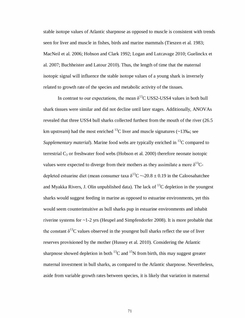
71

stable isotope values of Atlantic sharpnose as opposed to muscle is consistent with trends

seen for liver and muscle in fishes, birds and marine mammals (Tieszen et al. 1983;

MacNeil et al. 2006; Hobson and Clark 1992; Logan and Lutcavage 2010; Guelinckx et

al. 2007; Buchheister and Latour 2010). Thus, the length of time that the maternal

isotopic signal will influence the stable isotope values of a young shark is inversely

related to growth rate of the species and metabolic activity of the tissues.

In contrast to our expectations, the mean δ13C USS2-USS4 values in both bull

shark tissues were similar and did not decline until later stages. Additionally, ANOVAs

revealed that three USS4 bull sharks collected furthest from the mouth of the river (26.5

km upstream) had the most enriched 13C liver and muscle signatures (~13‰; see

Supplementary material). Marine food webs are typically enriched in 13C compared to

terrestrial C3 or freshwater food webs (Hobson et al. 2000) therefore neonate isotopic

values were expected to diverge from their mothers as they assimilate a more δ13C-

depleted estuarine diet (mean consumer taxa δ13C ~-20.8 ± 0.19 in the Caloosahatchee

and Myakka Rivers, J. Olin unpublished data). The lack of 13C depletion in the youngest

sharks would suggest feeding in marine as opposed to estuarine environments, yet this

would seem counterintuitive as bull sharks pup in estuarine environments and inhabit

riverine systems for ~1-2 yrs (Heupel and Simpfendorfer 2008). It is more probable that

the constant δ13C values observed in the youngest bull sharks reflect the use of liver

reserves provisioned by the mother (Hussey et al. 2010). Considering the Atlantic

sharpnose showed depletion in both 13C and 15N from birth, this may suggest greater

maternal investment in bull sharks, as compared to the Atlantic sharpnose. Nevertheless,

aside from variable growth rates between species, it is likely that variation in maternal

72

investment across shark species may also complicate establishing a single scar stage for

all species at which stable isotopes reflect the actual diet of young sharks.

For the bull shark, the lack of a decline in δ15N values with age could result from

(1) young sharks feeding on a diet with comparable δ15N values to their mothers or (2)

equivalent source δ15N values between young/mother habitats. Given the trend of

increasing body size-trophic level relationships in large predatory fish and sharks (Scharf

et al. 2000; Lucifora et al. 2009), mother-young feeding at the same trophic level would

seem unlikely. A more probable explanation is equivalent source δ15N values between

young/mother habitats. Baseline estuarine δ15N values in developed areas, like the

Caloosahatchee River estuary, are reportedly higher than coastal values (Heaton 1986)

therefore δ15N values of young individuals would be artificially inflated.

An unanticipated result was the lack of difference in the rate of maternal isotopic signal

loss among liver and muscle tissues of the bull shark. If we consider the previous

argument, that baseline δ15N signatures are similar between neonate and mother habitat,

then it is probable that we can extend this point to explain the similar δ15N values

between liver and muscle tissue of the bull shark. Liver tissue δ15N turns over

significantly faster than muscle tissue δ15N (MacNeil et al. 2006; Logan and Lutcavage

2010) Therefore, bull shark liver would reflect a diet representative of the enriched 15N

baseline, producing similar δ15N values to the slow turnover muscle tissue which would

reflect maternal reserves.

How the maternal stable isotope signal in near-term sharks and rays varies

between species or families adopting different reproductive strategies (i.e. oviparous,

ovoviviparous) is unknown. In teleost fishes, embryos are often depleted in 13C, as a

73

result of feeding on lipid-rich yolk, and isotopic values increase post-hatch with

assimilation of new dietary resources (Murchie and Power 2004; Witting et al. 2004).

Clearly, consideration of the maternal influence through the mother-young transfer of

maternal resources is thus necessary in any study using stable isotopes to assess diet,

foraging behaviour and/or habitat use of young animals.

Future research should focus on determining tissue-specific turnover rates of the

maternal signal in neonate to young-of-year sharks by applying exponential decay models

Hobson and Clark 1992; Fry and Arnold 1982). Through sampling pregnant females (and

associated newborn pups) and principal prey items in the diet of neonate/young-of-year

sharks within the nursery habitat, exponential decay models would facilitate an

examination of the rate of isotopic change or loss of maternal signature. This type of

model would provide a predictive framework for investigators to determine when stable

isotope values in tissues represent true diet and which juvenile animals could be sampled

without the influence from maternal reserves. Defining the maternal and dietary

endpoints of large sharks, however may be challenging when considering; (i) sampling

large pregnant females within a nursery ground is inherently difficult, (ii) defining the

dietary endpoint of neonatal sharks may be complex as many species undergo a rapid diet

shift with size, which may overlap the dietary endpoint of interest and (iii) for certain

shark species, juvenile and adult habitat overlap and therefore nursery habitat will not be

isotopically distinct, which complicates the definition of neonatal/young-of-year dietary

endpoints. Furthermore, the maternal isotopic signal is inherently variable (Barnes et al.

2008), both within a species and among species, and is influenced by whether the species

is a generalist or specialist feeder and/or if mothers forage in the same/variable habitat. A

74

single estimate of maternal isotopic tissue turnover would therefore not be applicable to

all species, but would guide field-sampling protocols.

It is difficult to draw definitive conclusions over the precise timing of tissue δ13C

and δ15N values achieving equilibrium with diet (i.e. exact USS or TL) when considering

that growth and maternal investment are species-specific. The declining trend of δ13C

values of both species for all three age measures, however, supports the hypothesis that

the maternal isotopic influence on stable isotope values of young sharks is evident for an

extended period of time after birth. Regardless of determining the exact stage of stable

isotope diet-equilibrium, our data provide the first practical approach for understanding

and measuring the loss of the maternal signal in stable isotope values of young sharks.

Until a comprehensive timeline for stable isotope tissue turnover in these age classes and

across species can be determined, we suggest a combination of USS and TL will enable

investigators to effectively sample animals that will provide accurate data for dietary and

food web studies.

REFERENCES

Barnes C. S., Jennings S., Polunin N.V.C. & Lancaster J.E. 2008. The importance of quantifying inherent variability when interpreting stable isotope field data. Oecologia 155:227–235. Bass A.J., D’Aubrey J.D. & Kistnasamy N. 1973. Sharks of the east coast of southern Africa. I. The genus Carcharhinus (Carcharhinidae). Oceanogr. Res. Inst. (Durban) Invest. Rep. (38), 100 p. Bligh E.G. & Dyer W.J. 1959. A rapid method of total lipid extraction and purification. Canadian Journal of Biochemistry and Physiology 37:911–917. Branstetter S. & Stiles R. 1987. Age and growth estimates of the bull shark, Carcharhinus leucas, from the northern Gulf of Mexico. Environmental Biology of Fishes 20:169–181.

75

Buchheister A. & Latour R.J. 2010. Turnover and fractionation of carbon and nitrogen stable isotopes in tissues of a migratory coastal predator, summer flounder (Paralichthys dentatus). Canadian Journal of Fisheries and Aquatic Science 67:445–461. Carlson J.K., Heupel M.R., Bethea D.M. & Hollensead L.D. 2008. Coastal habitat use and residency of juvenile Atlantic sharpnose sharks (Rhizoprionodon terraenovae). Estuaries and Coasts 31:931–940. Clark, E. & von Schmidt K. 1965. Sharks of the central Gulf coast of Florida. Bulletin of Marine Science 15:13–83. Caut S., Angulo E. & Courchamp F. 2009. Variation in discrimination factors (Δ15N and Δ13C): the effect of diet isotopic values and applications for diet reconstruction. Journal of Applied Ecology 46:443–453. Cortés E. 1999. Standardized diet compositions and trophic levels of sharks. ICES Journal of Marine Science 56:707–717. DeNiro M.J. & Epstein S. 1981. Influence of diet on the distribution of nitrogen isotopes in animals. Geochimica et Cosmochimica Acta 45:341–351. DeNiro M.J. & Epstein S. 1978. Influence of diet on the distribution of carbon isotopes in animals. Geochimica et Cosmochimica Acta 42:495–506. Duncan K.M. & Holland K.N. 2006. Habitat use, growth rates, and dispersal patterns of juvenile scalloped hammerhead sharks (Sphyrna lewini) in a nursery habitat. Marine Ecology Progress Series 312:211–221. Ducatez S., Dalloyau S., Richard P., Guinet C. & Cherel Y. 2008. Stable isotopes document winter trophic ecology and maternal investment of adult female southern elephant seals (Mirounga leonina) breeding in the Kerguelen Islands. Marine Biology 155:413–420. Fry B. & Arnold C. 1982. Rapid 13C/12C turnover during growth of brown shrimp (Panaeus aztecus). Oecologia 54:200–204. Guelinckx J., Maes J., Van Den Driessche P., Geysen B., Dehairs F. & Ollevier F. 2007. Changes in δ13Cand δ15N in different tissues of juvenile sand goby Pomatoschistus minutus: a laboratory diet-switch experiment. Marine Ecology Progress Series 341:205–215. Heaton T.H.E. 1986. Isotopic studies of nitrogen pollution in the hydrosphere and atmosphere: a review. Chemical Geology 59:87–102.

76

Heithaus M.R., Frid A., Wirsing A.J. & Worm B. 2008. Predicting ecological consequences of marine top predator declines. Trends in Ecology and Evolution 23:202–210. Heupel M.R. & Simpfendorfer C.S. 2008. Movement and distribution of young bull sharks Carcharhinus leucas, in a variable estuarine environment. Aquatic Biology 1:277–289. Hussey N.E., Wintner S.P., Dudley S.F.J., Cliff G., Cocks D.T. & MacNeil, M.A. 2010. Maternal investment and size-specific reproductive output in carcharhinid sharks. Journal of Animal Ecology 79:184–193. Hussey N.E., Cocks D.T., Dudley S.F.J., McCarthy I.D. & Wintner S.P. 2009. The condition conundrum: application of multiple condition indices to the dusky shark Carcharhinus obscurus. Marine Ecology Progress Series 380:199–212. Hobson K.A., Sirois J. & Gloutney M.L. 2000. Tracing nutrient allocation to reproduction with stable isotopes: A preliminary investigation using colonial waterbirds of Great Slave Lake. The Auk 117:760–774. Hobson K.A., Sease J.L., Merrick R.L. & Piatt J.F. 1997. Investigating trophic relationships of pinnipeds in Alaska and Washington using stable isotopes ratios of nitrogen and carbon. Marine Mammal Science 13:114–132. Hobson K.A. & Clark R.G. 1992 Assessing avian diets using stable isotopes I: turnover of 13C in tissues. Condor 94:181–184. Jenkins S.G., Partridge S.T., Stephenson T.R., Farley S.D. & Robbins C.T. 2001. Nitrogen and carbon isotope fractionation between mothers, neonates, and nursing offspring. Oecologia 129:336–341. Loefer J.K. & Sedberry G.R. 2003. Life history of the Atlantic sharpnose shark (Rhizoprionodon terraenovae; Richardson, 1836) off the southeastern United States. Fishery Bulletin 101:75–88. Logan, J.M. & Lutcavage M.E. 2010. Stable isotope dynamics in elasmobranch fishes. Hydrobiologia 644:231–244. Lucifora L.O., Garcia V.B., Menni R.C., Escalante A.H. & Hozbor N.M. 2009. Effects of body size, age and maturity stage on diet in a large shark: ecological and applied implications. Ecological Research 24:109–118. MacNeil M.A., Drouillard K.G. & Fisk A.T. 2006. Variable uptake and elimination of stable nitrogen isotopes between tissues in fish. Canadian Journal of Fisheries and Aquatic Science 63:345–353.

77

Matich P., Heithaus M.R. & Layman C.A. 2010. Size-based variation in inter-tissue comparisons of stable carbon and nitrogen isotopic signatures of bull sharks (Carcharhinus leucas) and tiger sharks (Galeocerdo cuvier). Canadian Journal of Fisheries and Aquatic Sciences 67:877–885. McMeans B.C., Olin J.A. & Benz G.W. 2009. Stable isotope comparisons between embryos and mothers of a placentatrophic shark species. Journal of Fish Biology 75:2464–2474. Minagawa M. & Wada E. 1984. Stepwise enrichment of 15N along food chains: further evidence and the relation between δ15N and animal age. Geochimica et Cosmochimica Acta 48:1135–1140. Murchie K.J. & Power M. 2004. Growth- and feeding-related isotopic dilution and enrichment patterns in young-of-the-year yellow perch (Perca flavescens). Freshwater Biology 49:41–54. Neer J.A., Thompson B.A. & Carlson J.K. 2005. Age and growth of Carcharhinus leucas in the northern Gulf of Mexico: incorporating variability in size at birth. Journal of Fish Biology 67:370–383. Oppel S. & Powell A.N. 2010. Carbon isotope turnover in blood as a measure of arrival time in migratory birds using isotopically distinct environments. Journal of Ornithology 151:123–131. Parsons G.R. 1985. Growth and age estimation of the Atlantic Sharpnose shark, Rhizoprionodon terraenovae: a comparison of techniques. Copeia 81:61–73. Peterson B.J. & Fry B. 1987. Stable isotopes in ecosystem studies. Annual Review: Ecology and Evolution Systematics 18:293–230. Pilgrim M.A. 2007. Expression of maternal isotopes in offspring: implications for interpreting ontogenetic shifts in isotopic composition of consumer tissues. Isotopes in Environmental Health Studies 43:155–163. Podlesak D.W., McWilliams S.R. & Hatch K.A. 2005. Stable isotopes in breath, blood, faeces and feathers can indicate intra-individual changes in the diet of migratory songbirds. Oecologia 142:501–510. Post D.M. 2002. Using stable isotopes to estimate trophic position: models, methods, and assumptions. Ecology 83:703–718. R Development Core Team. 2009. R: A language and environment for statistical computing. R Foundation for Statistical Computing, Vienna, Austria.

78

Sare D.T.J., Millar J.S. & Longstaffe F.J. 2005. Nitrogen- and carbon-isotope fractionation between mothers and offspring in red-backed voles (Clethrionomys gapperi). Canadian Journal of Zoology 83:712–716. Scharf F.S., Juanes F. & Rountree R.A. 2000. Predator size-prey size relationships of marine fish predators: interspecific variation and effects of ontogeny and body size on trophic-niche breadth. Marine Ecology Progress Series 208:229–248. Tieszen L.L., Boutton T.W., Tesdahl K.G. & Slade N.A. 1983. Fractionation and turnover of stable carbon isotopes in animal tissues: implications for δ13C analysis of diet. Oecologia 57:32–37. Vander Zanden M.J., Shuter B.J., Lester N.P. & Rasmussen J.B. 2000. Within- and among-population variation in the trophic position of a pelagic predator, lake trout (Salvelinus namaycush). Canadian Journal of Fisheries and Aquatic Science 57:725–731. Witting D.A., Chambers R.C., Bosley K.L. & Wainright S.C. 2004. Experimental evaluation of ontogenetic diet transitions in summer flounder (Paralichthys dentatus), using stable isotopes as diet tracers. Canadian Journal of Fisheries and Aquatic Science 61:2069–2084.

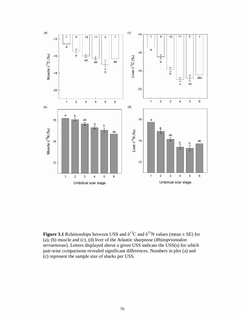
79

Figure 3.1 Relationships between USS and δ13C and δ15N values (mean ± SE) for (a), (b) muscle and (c), (d) liver of the Atlantic sharpnose (Rhizoprionodon terraenovae). Letters displayed above a given USS indicate the USS(s) for which pair-wise comparisons revealed significant differences. Numbers in plot (a) and (c) represent the sample size of sharks per USS.

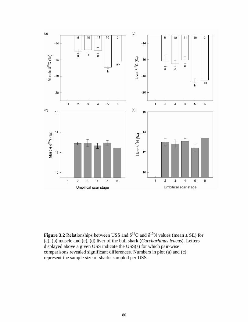
80

Figure 3.2 Relationships between USS and δ13C and δ15N values (mean ± SE) for (a), (b) muscle and (c), (d) liver of the bull shark (Carcharhinus leucas). Letters displayed above a given USS indicate the USS(s) for which pair-wise comparisons revealed significant differences. Numbers in plot (a) and (c) represent the sample size of sharks sampled per USS.

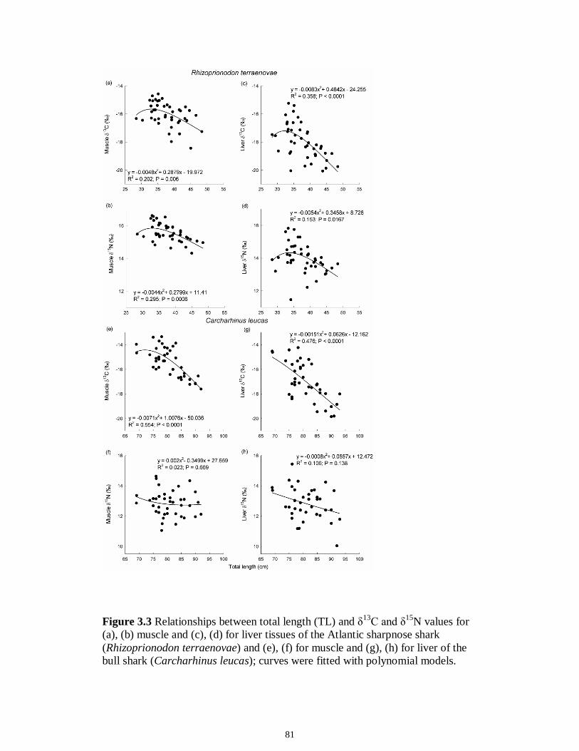
81

Figure 3.3 Relationships between total length (TL) and δ13C and δ15N values for (a), (b) muscle and (c), (d) for liver tissues of the Atlantic sharpnose shark (Rhizoprionodon terraenovae) and (e), (f) for muscle and (g), (h) for liver of the bull shark (Carcharhinus leucas); curves were fitted with polynomial models.

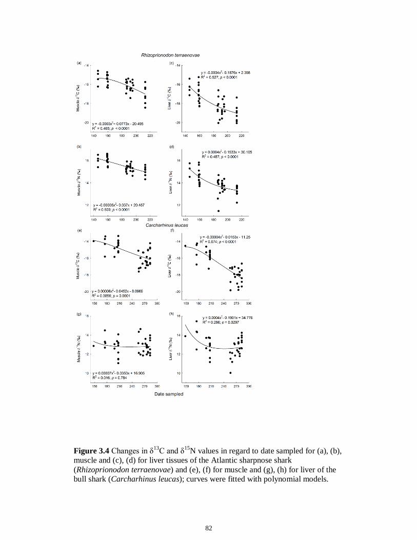
82

Figure 3.4 Changes in δ13C and δ15N values in regard to date sampled for (a), (b), muscle and (c), (d) for liver tissues of the Atlantic sharpnose shark (Rhizoprionodon terraenovae) and (e), (f) for muscle and (g), (h) for liver of the bull shark (Carcharhinus leucas); curves were fitted with polynomial models.

83

SUPPLEMENTAL MATERIAL

Sex did not have a significant influence on δ13C or δ15N of either tissue in

both species of shark (Table S3.1). Season, year, river and sampling location were

significant parameters influencing the stable isotope values of bull shark tissues,

particularly liver (p < 0.05; see Table S3.1). Sampling location by way of distance

from mouth of river was significant for δ13C of bull sharks. However, contrary to

our expectations, the results of the analysis indicated that three USS4 stage

individuals collected furthest from the mouth of the river (26.5 km) had enriched

13C signatures in liver and muscle (~13‰). Based on distance to the mouth and

work of Heupel & Simpfendorfer (2008) showing residency of bull sharks in

rivers for extended periods of time, it is unlikely that these individuals are

travelling 26.5 km to the mouth of the river to feed. Significant seasonal, annual

or river differences are not unexpected, as inherent variability within the system is

likely. Further, because individuals representing different life history stages were

combined for these analyses, differences were anticipated.

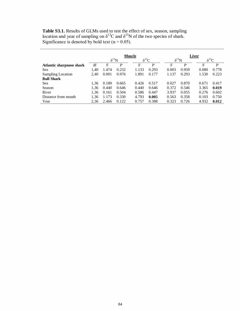
84

Table S3.1. Results of GLMs used to test the effect of sex, season, sampling location and year of sampling on δ13C and δ15N of the two species of shark. Significance is denoted by bold text (α = 0.05).

Muscle

Liver δ15N δ13C δ15N δ13C Atlantic sharpnose shark df F P F P F P F P Sex 1,40 1.474 0.232 1.133 0.293 0.003 0.959 0.080 0.778 Sampling Location 2,40 0.001 0.976 1.891 0.177 1.137 0.293 1.530 0.223 Bull Shark Sex 1,36 0.189 0.665 0.426 0.517 0.027 0.870 0.671 0.417 Season 1,36 0.440 0.646 0.440 0.646 0.372 0.546 3.365 0.019 River 1,36 0.161 0.504 0.586 0.447 3.937 0.055 0.276 0.602 Distance from mouth 1,36 1.173 0.330 4.793 0.005 0.563 0.358 0.103 0.750 Year 2,36 2.466 0.122 0.757 0.388 0.323 0.726 4.932 0.012

85

CHAPTER 4

ISOTOPIC RATIOS REVEAL MIXED SEASONAL VARIATION AMONG FISHES

FROM TWO SUBTROPICAL ESTUARINE SYSTEMS*

*Olin JA, Rush SA, MacNeil MA, Fisk AT. 2011. Isotopic ratios reveal mixed seasonal variation among fishes from two subtropical estuarine systems. Estuaries and Coasts doi: 10.1007/s12237-011-9467-6.

86

INTRODUCTION

Estuaries are highly productive and complex ecosystems that derive organic

carbon from a combination of sources (Bouillon et al. 2004; Peterson and Howarth 1987).

As a result, estuaries serve as nursery, rearing and feeding grounds for a diverse

assemblage of both resident and transient fish and invertebrate species (e.g., Beck et al.

2001). This complexity makes characterizing feeding relationships and dietary resource

partitioning in these systems especially challenging, particularly when considering that

body sizes of some individual consumer species can range over an order of magnitude

(Rountree and Able 1992) and that trophic roles can vary with ontogeny (Wilson and

Sheaves 2001).

The use of stable isotopes of nitrogen (δ15N), carbon (δ13C) and sulfur (δ34S) to

characterize dietary resources has become commonplace in studies of feeding ecology, as

they provide a time-integrated perspective of a consumer’s diet (Peterson and Fry 1987).

Specifically, δ15N values are used in determining the relative trophic position of a

consumer (Minagawa and Wada 1984) and δ13C and δ34S values have found application

in determining basal organic matter sources incorporated into a consumer’s diet (Peterson

and Fry 1987). Changes in δ15N in particular, can be attributed to either a trophic level

shift (i.e. feeding on more 15N enriched or depleted prey) or to a change in organic matter

sources supplementing the diet (i.e. pelagic to terrestrial-derived organic matter) or both

(Peterson and Howarth 1987). Thus applying δ13C and δ34S with δ15N in combination can

help to distinguish the potentially wide range of dietary resources available to consumers

(Connolly et al. 2004; Peterson and Howarth 1987).

87

Body size has long been recognized as influential on the structural and functional

complexity of aquatic food webs (Elton 1927). Size-based shifts in dietary resources,

reflecting the changing role of an organism within its community, are widespread in

aquatic species, including invertebrates (Cherel et al. 2009; Hoeninghaus and Davis

2007), teleosts (Deudero et al. 2004; Greenwood et al. 2010; Kolasinski et al. 2009),

marine turtles (Godley et al. 1998) and marine mammals (Newsome et al. 2009). Such

size-based differences often explain variation in stable isotope composition between

species (Akin and Winemiller 2008), and among conspecifics within a population

(Davenport and Bax 2002; Jennings et al. 2002). However, the ability to detect size-based

isotopic variation is often limited (Galván et al. 2010), as sampling the range of body

sizes needed to account for ontogenetic differences in the feeding ecology of consumers

can be difficult. This is particularly relevant in estuarine ecosystems, as high levels of

spatial and temporal variability in the physical and chemical properties (Deegan and

Garritt 1997; Abrantes and Sheaves 2010) influence the age class composition of species

at any particular time.

Size-dependent temporal variation in δ15N and δ13C has been observed in coastal

and open-water marine organisms (Goering et al. 1990; Jennings et al. 2008). Although

these observations were largely noted in lower trophic level species, such as zooplankton

and invertebrates, body size-related temporal variation has been identified in fishes

(Vizzini and Mazzola 2003). However, evidence against size- and temporal-based

isotopic shifts has been reported within estuarine consumers that indicated a dietary shift

with size, based on stomach content analyses (Wilson et al. 2009). Detection of temporal

variation in a consumer’s isotopic values however, is in part dependent on the lag

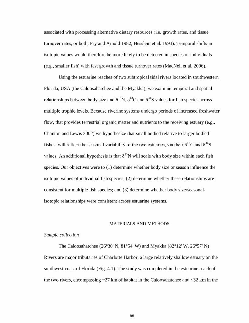
88

associated with processing alternative dietary resources (i.e. growth rates, and tissue

turnover rates, or both; Fry and Arnold 1982; Hesslein et al. 1993). Temporal shifts in

isotopic values would therefore be more likely to be detected in species or individuals

(e.g., smaller fish) with fast growth and tissue turnover rates (MacNeil et al. 2006).

Using the estuarine reaches of two subtropical tidal rivers located in southwestern

Florida, USA (the Caloosahatchee and the Myakka), we examine temporal and spatial

relationships between body size and δ15N, δ13C and δ34S values for fish species across

multiple trophic levels. Because riverine systems undergo periods of increased freshwater

flow, that provides terrestrial organic matter and nutrients to the receiving estuary (e.g.,

Chanton and Lewis 2002) we hypothesize that small bodied relative to larger bodied

fishes, will reflect the seasonal variability of the two estuaries, via their δ13C and δ34S

values. An additional hypothesis is that δ15N will scale with body size within each fish

species. Our objectives were to (1) determine whether body size or season influence the

isotopic values of individual fish species; (2) determine whether these relationships are

consistent for multiple fish species; and (3) determine whether body size/seasonal-

isotopic relationships were consistent across estuarine systems.

MATERIALS AND METHODS

Sample collection

The Caloosahatchee (26°30' N, 81°54' W) and Myakka (82°12' W, 26°57' N)

Rivers are major tributaries of Charlotte Harbor, a large relatively shallow estuary on the

southwest coast of Florida (Fig. 4.1). The study was completed in the estuarine reach of

the two rivers, encompassing ~27 km of habitat in the Caloosahatchee and ~32 km in the

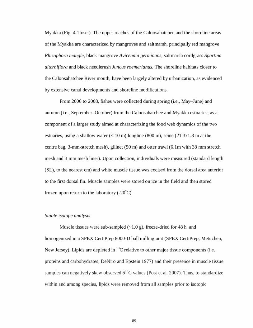
89

Myakka (Fig. 4.1Inset). The upper reaches of the Caloosahatchee and the shoreline areas

of the Myakka are characterized by mangroves and saltmarsh, principally red mangrove

Rhizophora mangle, black mangrove Avicennia germinans, saltmarsh cordgrass Spartina

alterniflora and black needlerush Juncus roemerianus. The shoreline habitats closer to

the Caloosahatchee River mouth, have been largely altered by urbanization, as evidenced

by extensive canal developments and shoreline modifications.

From 2006 to 2008, fishes were collected during spring (i.e., May–June) and

autumn (i.e., September–October) from the Caloosahatchee and Myakka estuaries, as a

component of a larger study aimed at characterizing the food web dynamics of the two

estuaries, using a shallow water (< 10 m) longline (800 m), seine (21.3x1.8 m at the

centre bag, 3-mm-stretch mesh), gillnet (50 m) and otter trawl (6.1m with 38 mm stretch

mesh and 3 mm mesh liner). Upon collection, individuals were measured (standard length

(SL), to the nearest cm) and white muscle tissue was excised from the dorsal area anterior

to the first dorsal fin. Muscle samples were stored on ice in the field and then stored

frozen upon return to the laboratory (-20°C).

Stable isotope analysis

Muscle tissues were sub-sampled (~1.0 g), freeze-dried for 48 h, and

homogenized in a SPEX CertiPrep 8000-D ball milling unit (SPEX CertiPrep, Metuchen,

New Jersey). Lipids are depleted in 13C relative to other major tissue components (i.e.

proteins and carbohydrates; DeNiro and Epstein 1977) and their presence in muscle tissue

samples can negatively skew observed δ13C values (Post et al. 2007). Thus, to standardize

within and among species, lipids were removed from all samples prior to isotopic

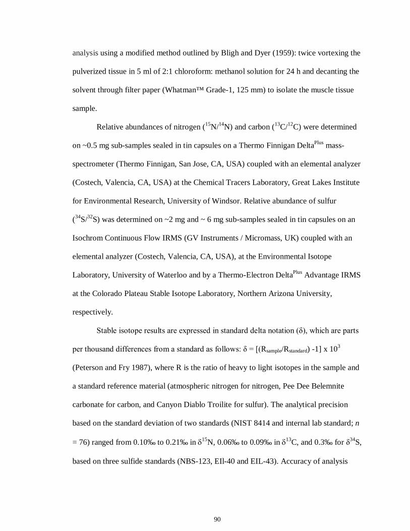
90

analysis using a modified method outlined by Bligh and Dyer (1959): twice vortexing the

pulverized tissue in 5 ml of 2:1 chloroform: methanol solution for 24 h and decanting the

solvent through filter paper (Whatman™ Grade-1, 125 mm) to isolate the muscle tissue

sample.

Relative abundances of nitrogen (15N/14N) and carbon (13C/12C) were determined

on ~0.5 mg sub-samples sealed in tin capsules on a Thermo Finnigan DeltaPlus mass-

spectrometer (Thermo Finnigan, San Jose, CA, USA) coupled with an elemental analyzer

(Costech, Valencia, CA, USA) at the Chemical Tracers Laboratory, Great Lakes Institute

for Environmental Research, University of Windsor. Relative abundance of sulfur

(34S/32S) was determined on ~2 mg and ~ 6 mg sub-samples sealed in tin capsules on an

Isochrom Continuous Flow IRMS (GV Instruments / Micromass, UK) coupled with an

elemental analyzer (Costech, Valencia, CA, USA), at the Environmental Isotope

Laboratory, University of Waterloo and by a Thermo-Electron DeltaPlus Advantage IRMS

at the Colorado Plateau Stable Isotope Laboratory, Northern Arizona University,

respectively.

Stable isotope results are expressed in standard delta notation (δ), which are parts

per thousand differences from a standard as follows: δ = [(Rsample/Rstandard) -1] x 103

(Peterson and Fry 1987), where R is the ratio of heavy to light isotopes in the sample and

a standard reference material (atmospheric nitrogen for nitrogen, Pee Dee Belemnite

carbonate for carbon, and Canyon Diablo Troilite for sulfur). The analytical precision

based on the standard deviation of two standards (NIST 8414 and internal lab standard; n

= 76) ranged from 0.10‰ to 0.21‰ in δ15N, 0.06‰ to 0.09‰ in δ13C, and 0.3‰ for δ34S,

based on three sulfide standards (NBS-123, EIl-40 and EIL-43). Accuracy of analysis

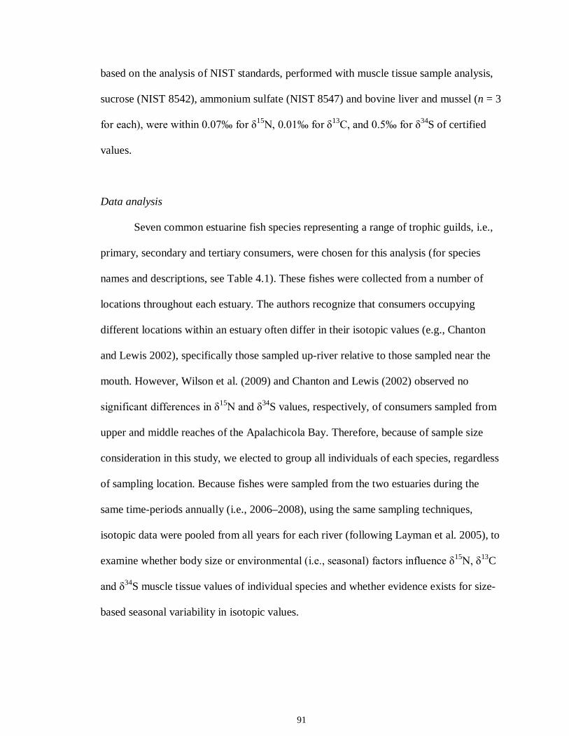
91

based on the analysis of NIST standards, performed with muscle tissue sample analysis,

sucrose (NIST 8542), ammonium sulfate (NIST 8547) and bovine liver and mussel (n = 3

for each), were within 0.07‰ for δ15N, 0.01‰ for δ13C, and 0.5‰ for δ34S of certified

values.

Data analysis

Seven common estuarine fish species representing a range of trophic guilds, i.e.,

primary, secondary and tertiary consumers, were chosen for this analysis (for species

names and descriptions, see Table 4.1). These fishes were collected from a number of

locations throughout each estuary. The authors recognize that consumers occupying

different locations within an estuary often differ in their isotopic values (e.g., Chanton

and Lewis 2002), specifically those sampled up-river relative to those sampled near the

mouth. However, Wilson et al. (2009) and Chanton and Lewis (2002) observed no

significant differences in δ15N and δ34S values, respectively, of consumers sampled from

upper and middle reaches of the Apalachicola Bay. Therefore, because of sample size

consideration in this study, we elected to group all individuals of each species, regardless

of sampling location. Because fishes were sampled from the two estuaries during the

same time-periods annually (i.e., 2006–2008), using the same sampling techniques,

isotopic data were pooled from all years for each river (following Layman et al. 2005), to

examine whether body size or environmental (i.e., seasonal) factors influence δ15N, δ13C

and δ34S muscle tissue values of individual species and whether evidence exists for size-

based seasonal variability in isotopic values.

92

Body size and seasonal relationships were analyzed using linear mixed-effects

models fit using restricted maximum likelihood in the lme4 package in R (R Core

Development Team 2009; Bates and Maechler 2010). Prior to analysis all stable isotope

data were tested for normality using quantile-quantile probability plots and log-

transformed where appropriate. We developed a set of three candidate models with

estuary as the random effect and body size and season as fixed effects: a model with no

predictors (Null model; Isotope = γ0 + β0 + ε), and models including the body size

(Isotope = γ0 + γ1Body Size + β0 + ε) and seasonal (Isotope = γ0 + γ2Season + β0 + ε)

predictors suspected of influencing isotopic values of the fishes collected during the

sampling period. All candidate models were implemented for each species. An

examination of the probability plots of residuals from all candidate models relating site-

specific species isotopic values to species body size and season sampled, indicated that

candidate models fit adequately, and quantile-quantile plots showed data to be generally-

described by normally distributed errors for all fishes.

Model selection was based on Akaike’s Information Criterion (AIC; Akaike

1973) with small-sample bias adjustment (AICc; Hurvich and Tsai 2002). In determining

model AICc values, both random (i.e., estuary) and fixed (i.e., body size and season)

effects were counted as unique parameters and the number of observations used to

compute the log-likelihood were used in calculating AICc. Models were ranked and

compared using AICc weights and ΔAICc, where AICc weights measure the weight in

support of the model given the data and ΔAICc is the relative difference between the top

ranked model and each alternative model. In most cases the model with the lowest AICc

value was considered the best-supported model. However, when the AICc of several

93

models differed by ≤ 2, we considered these models to be equally parsimonious.

Additionally, if the number of parameters (K) in comparative models differed by 1, then

model selection was based on the log-likelihood, with the best supported model having

the lower log-likelihood (Burnham and Anderson 2002). Akaike weights (wi) were

calculated to interpret the weight of evidence for the best fitting model with evidence

ratios used to compare among models (Johnson and Omland 2004). For the best

supported model, parameter estimates and associated 95% confidence intervals (CIs)

were determined using the HPDinterval function provided in the lme4 package in R. For

each estimated parameter, predictors were considered significant if the confidence

interval did not contain zero. To test the effect of body size and season among estuaries,

we calculated the intraclass correlation coefficients (ICC), reflecting the proportion of

variance attributable to each level of the model (see Raudenbush and Bryk 2002; Elgee et

al. 2010). The ICC approaches 1 when the between-estuary variation is large relative to

the within-estuary variation and this coefficient has a 0 value when the within-estuary

variation equals the between-estuary variation.

RESULTS

Results from the candidate models used to describe the relationships between

δ15N and season-body size effects in the fishes sampled from both the Caloosahatchee

and Myakka estuaries indicated that the null model was the top-ranked model for five out

of seven species (i.e., there was no effect of season or body size) (Table 4.2; see Table

4S.1 Supplemental Material for full model comparisons for δ15N). However, evidence

based on model comparisons indicated that season was the most plausible model

94

describing the δ15N values of two species; Mugil cephalus, and Chaetodipterus faber

(Table 4.2). The parameter estimates for season were significant for both species (Fig.

4.2A; i.e. zero was not included within the CI) and evidence ratios estimated for these

species, indicate that the model that included season was 48.5 and 47 times more likely

than the model that included body size, respectively (see Table 4S.1). Model comparisons

indicated depletion in 15N between spring and autumn in C. faber (Table 4.1), whereas M.

cephalus enriched in 15N between spring and autumn.

Relationships between season and body size and δ13C, favored the null model for

four of the seven species in this study (Table 4.2; see Table 4S.2Supplemental Material

for full model comparisons for δ13C), suggesting limited evidence for size or seasonal

effects in the data. The most plausible model describing the δ13C values of Bagre

marinus, M. cephalus and Eugerres plumieri included season (Table 4.2). However,

confidence intervals that overlapped zero suggest there is only weak evidence of a

seasonal effect on the δ13C values of B. marinus (Fig. 4.2B). Carbon isotope values of E.

plumieri were generally lower in the autumn relative to the spring, and evidence ratios

indicated the model that included season was 2.8 times more likely than the model that

included body size. This was also the case for the δ13C values of M. cephalus; a clear

depletion in 13C in the autumn (Table 4.1; Fig. 4.2B).

Seasonal variability was identified in four of the seven species using δ34S (Table

4.2; see Table 4S.3Supplemental Material for full model comparisons for δ34S). The

support for C. faber, B. marinus and Ariopsis felis was strong (Fig. 4.2C) with the model

that included season being 30, 4.1 and 32 times more likely than the model containing

body size, respectively (see Table 4S.3). Moreover, depletion in 34S from spring to

95

autumn was evident for the three species (Table 4.1) further supporting a seasonal effect

in both estuaries (Fig. 2C). Alternatively, the best model describing the sulfur isotopes of

E. plumieri indicated a general enrichment in 34S in the autumn relative to spring (Fig.

4.2C). Intraclass correlation coefficients indicated that the proportion of variance

attributable to the seasonal variation within-estuary (61–100%) was greater than the

proportion attributable to season between-estuary (0–39%) in all isotopic comparisons in

all species, suggesting that seasonal variability was similar between our study locations.

DISCUSSION

Our results provide evidence that for most species examined, season is the

dominant influence on isotopic values within the Caloosahatchee and Myakka estuaries

relative to body size of the fishes sampled here. Our results are in accordance with those

of Wilson et al. (2009), supporting the fact that body size is not an important determinant

of isotopic enrichment in estuarine fishes. However, there was evidence for seasonal

variability in isotopic values in fish species that spanned several trophic levels and across

spatially distinct systems. It is well known that many fishes undergo size-based or

ontogenetic changes in diet, and thereby occupy a number of trophic levels in the course

of their life history (Winemiller 1990). The absence of intra-specific association between

δ15N, δ13C, δ34S, and body size, suggests that these estuarine fish species do not undergo

size-based dietary changes within the size ranges sampled here. However, the seasonal

shift in isotopic values supports the finding of Polis and Strong (1996) in that the relative

trophic positions of species, whether attributable to a change in diet or a shift in isotopic

values of organic matter sources in food webs, are dynamic rather than fixed. The

96

estuarine fishes examined in the current study exhibit plasticity in their feeding strategy,

as they are clearly responding to changes in production source. Differing δ15N, δ13C and

δ34S values between seasons, suggests that seasonal variability influences the isotopic

values of estuarine fishes, and thus the species interactions and the food web structure of

these estuarine systems.

Body size variability

The absence of body-size based- δ15N relationships in the fishes sampled likely

result from (1) dietary preferences of these fishes not shifting within the range of body

sizes sampled, (2) the fishes do shift to alternative diets with size, yet the isotope ratios of

the new diet are similar to the former and are not reflected in isotopic distinctions, or (3)

that spatial and temporal variation in isotopic signatures of prey negate any size-based

relationships in higher trophic level species (Vander Zanden et al. 2000). Deudero et al.

(2004) observed no size-based δ15N changes in fishes that fed primarily on small benthic

invertebrates, suggesting that although these fishes possess very diverse diets throughout

their lives, they likely select prey of relatively similar trophic level. Given the trend of

increasing body size-trophic level relationships in large predatory (Scharf et al. 2000) and

piscivorous fishes (Deudero et al. 2004), the lack of size-based δ15N relationships in the

fishes included in our study may be a consequence of the fact they are predominantly

secondary and tertiary consumers. As such, early life stages (i.e. larvae and young-of-

year) generally feed in the pelagic environment on zooplankton and switch to benthic

macro-invertebrates in later stages, thus significant size-based δ15N relationships would

likely have been evident from a broader range of sizes that including larval individuals

97

(Mittelbach and Persson 1998). Nonetheless, similar results for estuarine species of the

Apalachicola Bay, an estuary in northern Florida, have been observed (Wilson et al.

2009).

Galván et al. (2010) raised the point that, the absence of a size-based relationship

with δ15N often resulted from the statistical power being too low to detect a significant

relationship. This may be the case here, as both sample size and range of sizes sampled

were low for a number of species. Yet, given the assumptions for estimating the minimal

sample size required to analyze size based feeding relationships using δ15N (Galván et al.

2010), the body-size independent δ15N results for 57% of the focal species (4/7) were

sampled across size ranges that exceeded Galvan's suggested cutoff. Although, we are

confident in our relationships for the majority of species sampled, limited statistical

power suggests further sampling may be required for some species. For species that did

not meet the sample size minimum for each season, i.e., Mugil cephalus, Lagodon

rhomboides and Chaetodipterus faber, improvement in power can be achieved by

sampling a greater number of individuals over a broader size range, to confirm the

absence of size relationships with δ15N and seasonal shifts in isotopic values. However, it

is important to note that use of estuaries by fishes is often seasonally based (Sheaves et

al. 2010) and therefore sampling the entire size range of an individual species may not be

possible.

Body size-dependent shifts in isotope ratios that reflect a shift in a consumer’s

diet can be attributed to either a trophic level shift and/or changes in organic matter

source available to a consumer. However, in complex ecosystems, such as tropical

floodplain rivers, size-related isotopic shifts are less common than in temperate aquatic

98

habitats (Jennings et al. 2002), as multiple primary production sources support highly

variable trophic assemblages whose interactions may favor a diversification of size across

trophic levels (Layman et al. 2005). Our finding that neither δ13C nor δ34S was associated

with body size suggests the potential for absence of systematic shifts in organic matter

source use that could potentially obscure the δ15N trends with body size, lending support

to the lack of evidence of size-based isotopic shifts within our study systems.

Seasonal variability

Body-size dependent diet shifts have been shown to influence temporal variation

in aquatic food webs, particularly in highly seasonal systems (Winemiller 1990). Goering

et al. (1990) suggested that aside from primary producers, seasonal isotopic variability is

confined to relatively short-lived primary consumers because of relatively fast growth

and associated tissue turnover rates. This has been supported by studies examining the

influence of seasonal variation on producers and consumers (Jennings et al. 2008),

attributing the lack of evidence in secondary and tertiary consumers, to weak seasonal

variability of the system under examination and to the relatively slow rate of muscle

turnover in vertebrate species (MacAvoy et al. 2001). Despite these potential limitations,

seasonal variability was evident for all three isotopes employed in our study, a result

similar to those reported by Vizzini and Mazzola (2003) from a Mediterranean coastal

lagoon, and by Chanton and Lewis (2002) from the Apalachicola Bay.

Generally, with respect to δ13C and δ34S, the most depleted values were observed

in autumn. Although we did not characterize the primary producers of either estuary,

overall seasonal variability in δ13C (mean ± SE; spring, -19.6 ± 0.3‰ and -20.8 ± 0.4‰;

99

autumn, -20.6 ± 0.4‰ and -20.6 ± 0.3‰) and δ34S (mean ± SE; spring, 12.9 ± 0.3‰ and

12.7 ± 0.3‰; autumn, 10.3 ± 0.4‰ and 11.1 ± 0.3‰) of all fishes combined in the

Caloosahatchee and the Myakka respectively, was relatively low. Shifts in δ13C and δ34S

are however reflected in the fishes’ tissues likely indicating either movement to new

habitats or a shift in organic matter source associated with the transition of dry to wet

seasons in these estuaries. With the onset of the wet season, both rivers experience

increased freshwater flow from natural sources such as rain and subsequent watershed

drainage. This source of freshwater into the system could lead to consumers assimilating

a more mangrove/upland carbon and sulfur source. The autumnal shift in the sulfur

isotope ratios potentially reflects the input of upland/mangrove organic matters sources

into the estuaries. The fact that this shift was more evident in δ34S as opposed to δ13C

may be a consequence of sulfur sources being more distinguishable (i.e., sulfide vs.

sulfate). Interpreting δ13C values in estuarine organisms can often be difficult because a

mixture of terrestrial (∼27‰) and salt-marsh (∼13‰) organic matter sources can yield a

δ13C value similar to marine phytoplankton (∼21‰; Connelly et al. 2004; Peterson and

Fry 1987).

Seasonal variation in isotopic values was prevalent in the majority of fishes,

regardless of trophic position. This result has implications for the trophic roles of species

in estuarine food webs and the tools we use to identify these relationships within the food

web. One way that seasonal variation can influence our conceptual understanding of

trophic relationships within estuaries relates to the use of stable isotopes. Because tissue

turnover is related to growth and metabolism, rates can vary by species, tissue type and

body size. For instance, generally accepted estimates of isotopic turnover in muscle range

100

from less than a week for larval red drum (Sciaenops ocellatus; Herzka and Holt 2000) to

> 400 days in juvenile catfish (Ictalurus punctatus; MacAvoy et al. 2001) to > 500 days

for δ13C and > 300 days for δ15N in muscle tissues of juvenile sandbar sharks

(Carcharhinus plumbeus; Logan and Lutcavage 2010). Consideration of temporal

variability in isotope values must be taken into account in all species of the community,

despite the expected lag in tissue turnover rates, as shifts in prey resources or

environmental conditions can greatly alter isotopic signals.

Spatial variability

The seasonally driven isotopic trends were similar among conspecifics of the

Caloosahatchee and Myakka estuaries, as the proportion of variance attributable to

seasonal effects within-estuary was greater than that attributable to seasonal effects

between-estuary, despite the limitation of small sample size for some species. Arguably,

there is the potential that the similar seasonal trends observed here among the estuaries is

a result of small sample sizes and that more focused sampling would result in different

results. Estuarine consumers however, are known to exhibit omnivory and have the

ability to exploit peaks of prey abundance. Isotopic differences among conspecifics have

been identified at multiple spatial scales: among habitats within an estuary (Deegan and

Garritt 1997) and among neighboring estuaries (Griffin and Valiela 2001). Spatial

differences in isotopic values would indicate that fishes adopt site-specific feeding

strategies or the variability in the isotopic composition of prey resources. Similar trends

between conspecifics of the two rivers, therefore suggests that the seasonal factors

101

driving the isotopic dynamics of these fish species are of similar magnitude, and that the

fishes are responding to environmental factors in a comparable fashion.

We expected that the seasonal isotopic trends of the fishes examined here would

have differed over these moderate spatial scales. However, within the southeastern USA,

the magnitude of nutrient input entering into estuarine systems depends strongly on

riverine discharge and can vary seasonally (Dardeu et al. 1992). In southwest Florida,

many rivers are categorized as having the southern river flow pattern, i.e. a significant

proportion of riverine annual flow (~60%) is concentrated in the rainy season, which

generally occurs in the months of June-September (Kelly and Gore 2008). This is

particularly relevant to the Caloosahatchee and Myakka Rivers, and provides a rationale

for the similar seasonal trends exhibited between the two estuaries.

Conclusions

We have established that isotopic variation in the Caloosahatchee and Myakka

estuaries is influenced by seasonal differences as opposed to size based structuring within

fish species. Evidence of seasonal variability among fishes, across a range of trophic

levels, suggests that these fishes exhibit plasticity in feeding strategies that may afford

greater adaptive flexibility in response to specific changes in food availability resulting

from changes in environmental conditions. Likewise, the response of conspecifics

between the two estuaries is similar suggesting that the environmental influence on the

isotopic composition (δ13C and δ34S) of these estuarine fishes is of comparable

magnitude. These results further suggest that the trophic structure of these estuarine food

webs, as indicated by δ15N, is variable among seasons, a result that may be attributable to

102

the alteration in organic matter and/or nutrient sources associated with changes to

hydrological regime.

REFERENCES

Abrantes K. & Sheaves M. 2010. Importance of freshwater flow in terrestrial-aquatic energetic connectivity in intermittently connected estuaries of tropical Australia. Marine Biology 157:2071–2086. Akaike H. 1973. Information theory and an extension of the maximum likelihood principle. In International Symposium on Information Theory, 2nd Edition, ed. B.N. Petran, and F. Csaki, 267–281. Akademiaiiadi, Budapest. Akin A. & Winemiller K.O. 2008. Body size and trophic position in a temperate estuarine food web. Acta Oecologia 33:144–153. Bates D. & Maechler M. 2010. Linear mixed-effects models using S4 class in R. 12/2010. Beck M.W., Heck K.L., Able K.W., Childers D.L., Eggleston D.B., Gillanders B.M., Halpern B., Hays C.G., Hoshino K., Minello T.J., Orth R.J., Sheridan P.F. & Weinstein M.P. 2001. The identification, conservation and management of estuarine and marine nurseries for fish and invertebrates. Bioscience 51:633–641. Bligh E.G. & Dyer W.J. 1959. A rapid method of total lipid extraction and purification. Canadian Journal of Biochemistry and Physiology 37:911–917. Bouillon S., Moens T., Overmeer I., Koedam N. & Dehairs F. 2004. Resource utilization patterns of epifauna from mangrove forests with contrasting inputs of local versus imported organic matter. Marine Ecology Progress Series 278:77–88. Burnham K.P. & Anderson D.R. 2002. Model Selection and Multimodel Inference: A Practical Information–Theoretic Approach, 488. New York: Springer–Verlag. Chanton J. & Lewis F.G. 2002. Examination of coupling between primary and secondary production in a river-dominated estuary: Apalachicola Bay. Limnology and Oceanography 47:683–697. Cherel Y., Fontaine C, Jackson G.D, Jackson C.H. & Richard P. 2009. Tissue, ontogenetic and sex-related differences in δ13C and δ15N values of the oceanic squid Todarodes filippovae (Cephalopoda: Ommastrephidae). Marine Biology 156:699–708.

103

Connolly R.M., Guest M.A, Mellville A.J. & Oakes J.M. 2004. Sulfur stable isotopes separate producers in marine food web analysis. Oecologia 138:161–167. Dardeu M.R., Modlin R.F, Schroeder W.W. & Stout J.P. 1992. Estuaries. In Biodiversity of the southeastern United States: Aquatic communities (C.T. Hackney, S.M. Adams, and W.M. Martin Eds.), 614–744. New York: Wiley. Davenport S.R. & Bax N.J. 2002. A trophic study of a marine ecosystem off south-eastern Australia using stable isotopes of carbon and nitrogen. Canadian Journal of Fisheries and Aquatic Sciences 59:514–530. Deegan L.A. & Garritt R.H. 1997. Evidence for spatial variability in estuarine food webs. Marine Ecology Progress Series 147:31–47. DeNiro M.J. & Epstein S. 1977. Mechanism of carbon isotope fractionation associated with lipid synthesis. Science 197:261–263. Deudero S., Pinnegar J.K, Polunin N.V.C., Morey G. & Morales-Nin B. 2004. Spatial variation and ontogenetic shifts in the isotopic composition of Mediterranean littoral fishes. Marine Biology 145:971–981. Elgee K.E., Evans J.P., Ramnarine I.W., Rush S.A. & Pitcher T.E. 2010. Geographic variation in sperm traits reflects predation risk and natural rates of multiple paternity in the guppy. Journal of Evolutionary Biology 23:1331–1338. Elton C.S. 1927. Animal Ecology. Sidgwick and Jackson, London, 207 pp. Froese R. & Pauly D. 2010. FishBase. Available at: www.fishbase.org. 12/2010. Fry B. & Arnold C. 1982. Rapid 13C/12C turnover during growth of brown shrimp (Penaeus aztecus). Oecologia 54:200–204. Galván D.E., Sweeting C.J. & Reid W.D.K. 2010. Power of stable isotope techniques to detect size-based feeding in marine fishes. Marine Ecology Progress Series 407:271–278. Godley B.J., Thompson D.R., Waldron S. & Furness R.W. 1998. The trophic status of marine turtles as determined by stable isotope analysis. Marine Ecology Progress Series 166:277–284. Goering J., Alexander V. & Haubenstock N. 1990. Seasonal variability of stable carbon and nitrogen isotope ratios of organisms in a North Pacific Bay. Estuarine, Coastal and Shelf Science 30:239–260. Greenwood N.D., Sweeting C.J. & Polunin N.V.C. 2010. Elucidating the trophodynamics of four coral reef fishes of the Solomon Islands using δ15N and δ13C. Coral Reefs 29:785–792.

104

Griffin M.P.A. & Valiela I. 2001. δ15N isotope studies of life history and trophic position of Fundulus heteroclitus and Menidia menidia. Marine Ecology Progress Series 214:299–305. Hesslein R.H., Hallard K.A. & Ramlal P. 1993. Replacement of sulfur, carbon and nitrogen in tissues of growing broad whitefish (Coregonus nasus) in response to a change in diet traced by δ34S, δ13C and δ15N. Canadian Journal of Fisheries and Aquatic Sciences 50:2071–2076. Herzka S.Z. & Holt G.J. 2000. Changes in isotopic composition of red drum (Sciaenops ocellatus) larvae in response to dietary shifts: potential applications to settlement studies. Canadian Journal of Fisheries and Aquatic Sciences 57:137–147. Hoeinghaus D.J. & Davis S.E. 2007. Size-based trophic shifts of saltmarsh dwelling blue crabs elucidated by dual stable C and N isotope analyses. Marine Ecology Progress Series 334:199–204. Hurvich C.M. & Tsai C. 1989. Regression and time series model selection in small samples. Biometrika 76:297–307. Jennings S., Maxwell T.A.D., Schratzberger M. & Milligan S.P. 2008. Body-size dependent temporal variation in nitrogen stable isotope ratios in food webs. Marine Ecology Progress Series 370:199–206. Jennings S., Pinnegar J.K, Polunin N.V.C. & Warr K.J. 2002. Linking size-based and trophic analyses of benthic community structure. Marine Ecology Progress Series 226:77–85. Johnson J.B. & Omland K.S. 2004. Model selection in ecology and evolution. Trends in Ecology and Evolution 19:101–108. Kelly M.H. & Gore J.A. 2008. Florida river flow patterns and the Atlantic multidecadal oscillation. River Research and Applications 24:598–616. Kolasinski J., Frouin P., Sallon A., Rogers K., Bruggeman H.J. & Potier M. 2009. Feeding ecology and ontogenetic diet shift of yellowstripe goatfish Mulloidichthys flavolineatus (Mullidae) at Reunion Island, SW Indian Ocean. Marine Ecology Progress Series 386:181–195. Layman C.A., Winemiller K.O, Arrington D.A. & Jepsen D.B. 2005. Body size and trophic position in a diverse tropical food web. Ecology 86:2530–2535. Logan J.M. & Lutcavage M.E. 2010. Stable isotope dynamics in elasmobranch fishes. Hydrobiologia 644:231–244.

105

MacAvoy S.E., Macko S.A. & Garman G.C. 2001. Isotopic turnover in aquatic predators: quantifying the exploitation of migratory prey. Canadian Journal of Fisheries and Aquatic Sciences 58:923–932. MacNeil M.A., Drouillard K.G. & Fisk A.T. 2006. Variable uptake and elimination of stable nitrogen isotopes between tissues in fish. Canadian Journal of Fisheries and Aquatic Sciences 63:345–353. Minagawa M. & Wada E. 1984. Stepwise enrichment of 15N along food chains: further evidence and the relation between δ15N and animal age. Geochimica et Cosmochimica Acta 48:1135–1140. Mittelbach G.G. & Persson L. 1998. The ontogeny of piscivory and its ecological consequences. Canadian Journal of Fisheries and Aquatic Sciences 55:1454–1465. Newsome S.D., Etnier M.A., Monson D.H. & Fogel M.L. 2009. Retrospective characterization of ontogenetic shifts in killer whale diets via δ13C and δ15N analysis of teeth. Marine Ecology Progress Series 374:229–242. Peterson B.J. & Fry B. 1987. Stable isotopes in ecosystem studies. Annual Review: Ecology Evolution and Systematics 18:293–320. Peterson B.J. & Howarth R.W. 1987. Sulfur, carbon, and nitrogen isotopes used to trace organic matter flow in the salt-marsh estuaries of Sapelo Island, Georgia. Limnology and Oceanography 32:1195–1213. Platell M.E., Orr P.A. & Potter I.C. 2006. Inter- and intraspecific partitioning of food resources by six large and abundant fish species in a seasonally open estuary. Journal of Fish Biology 69:243–262. Polis G.A. & Strong D.A. 1996. Food web complexity and community dynamics. The American Naturalist 147:813–846. Olin J.A., Hussey N.E., Fritts M., Heupel M.R., Simpfendorfer C.A., Poulakis G.R. & Fisk A.T. 2011. Maternal meddling in neonatal sharks: implication for interpreting stable isotopes in young animals. Rapid Communications in Mass Spectrometry 25:1008–1016. Post D.M., Layman C.A, Arrington D.A., Takimoto G., Quattrochi J. & Montaña C.G. 2007. Getting to the fat of the matter: models, methods and assumptions for dealing with lipids in stable isotope analyses. Oecologia 152:179–189. Post D.M. 2002. Using stable isotopes to estimate trophic position: Models, methods and assumptions. Ecology 83:703–718. R Development Core Team. 2009. R: A language and environment for statistical computing. R Foundation for Statistical Computing, Vienna, Austria.

106

Raudenbush S.W. & Bryk A.S. 2002. Hierarchical linear models: Applications and data analysis methods. Sage Publications, London, 491 pp. Rountree R.A. & Able K.W. 1992. Fauna of polyhaline subtidal marsh creeks in southern New Jersey: Composition, abundance biomass. Estuaries 15:171–185. Scharf F.S., Juanes F. & Rountree R.A. 2000. Predator size-prey size relationships of marine fish predators: inter-specific variation and effects of ontogeny and body size on trophic-niche breadth. Marine Ecology Progress Series 208:229–248. Sheaves M., Johnston R. & Connolly R.M. 2010. Temporal dynamics of fish assemblages of natural and artificial tropical estuaries. Marine Ecology Progress Series 410:143–157. Vander Zanden M.J., Shuter B.J., Lester N.P. & Rasmussen J.B. 2000. Within- and among-population variation in the trophic position of a pelagic predator, lake trout (Salvelinus namaycush). Canadian Journal of Fisheries and Aquatic Science 57:725–731. Vizzini S. & Mazzola A. 2003. Seasonal variations in the stable carbon and nitrogen isotope ratios (13C/12C and 15N/14N) of primary producers and consumers in a western Mediterranean coastal lagoon. Marine Biology 142:1009–1018. Wilson R.M., Chanton J., Lewis G. & Nowacek D. 2009. Isotopic variation (δ15N, δ13C and δ34S) with body size in post-larval estuarine consumers. Estuarine, Coastal and Shelf Science 83:307–312. Wilson J.P. & Sheaves M. 2001. Short-term temporal variation in taxonomic composition and trophic structure of a tropical estuarine fish assemblage. Marine Biology 139:787–796. Winemiller K.O. 1990. Spatial and temporal variation in tropical fish trophic networks. Ecological Monographs 60:331–367.

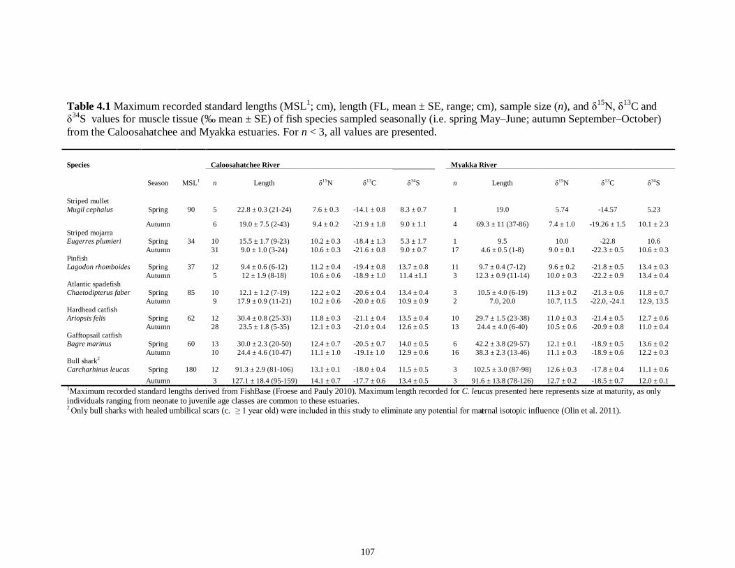
107

Table 4.1 Maximum recorded standard lengths (MSL1; cm), length (FL, mean ± SE, range; cm), sample size (n), and δ15N, δ13C and δ34S values for muscle tissue (‰ mean ± SE) of fish species sampled seasonally (i.e. spring May–June; autumn September–October) from the Caloosahatchee and Myakka estuaries. For n < 3, all values are presented.

Species

Caloosahatchee River Myakka River

Season MSL1 n Length δ15N δ13C δ34S n Length δ15N δ13C δ34S

Striped mullet Mugil cephalus Spring 90 5 22.8 ± 0.3 (21-24) 7.6 ± 0.3 -14.1 ± 0.8 8.3 ± 0.7 1 19.0 5.74 -14.57 5.23

Autumn 6 19.0 ± 7.5 (2-43) 9.4 ± 0.2 -21.9 ± 1.8 9.0 ± 1.1 4 69.3 ± 11 (37-86) 7.4 ± 1.0 -19.26 ± 1.5 10.1 ± 2.3 Striped mojarra Eugerres plumieri Spring 34 10 15.5 ± 1.7 (9-23) 10.2 ± 0.3 -18.4 ± 1.3 5.3 ± 1.7 1 9.5 10.0 -22.8 10.6 Autumn 31 9.0 ± 1.0 (3-24) 10.6 ± 0.3 -21.6 ± 0.8 9.0 ± 0.7 17 4.6 ± 0.5 (1-8) 9.0 ± 0.1 -22.3 ± 0.5 10.6 ± 0.3 Pinfish Lagodon rhomboides Spring 37 12 9.4 ± 0.6 (6-12) 11.2 ± 0.4 -19.4 ± 0.8 13.7 ± 0.8 11 9.7 ± 0.4 (7-12) 9.6 ± 0.2 -21.8 ± 0.5 13.4 ± 0.3 Autumn 5 12 ± 1.9 (8-18) 10.6 ± 0.6 -18.9 ± 1.0 11.4 ±1.1 3 12.3 ± 0.9 (11-14) 10.0 ± 0.3 -22.2 ± 0.9 13.4 ± 0.4 Atlantic spadefish Chaetodipterus faber Spring 85 10 12.1 ± 1.2 (7-19) 12.2 ± 0.2 -20.6 ± 0.4 13.4 ± 0.4 3 10.5 ± 4.0 (6-19) 11.3 ± 0.2 -21.3 ± 0.6 11.8 ± 0.7 Autumn 9 17.9 ± 0.9 (11-21) 10.2 ± 0.6 -20.0 ± 0.6 10.9 ± 0.9 2 7.0, 20.0 10.7, 11.5 -22.0, -24.1 12.9, 13.5 Hardhead catfish Ariopsis felis Spring 62 12 30.4 ± 0.8 (25-33) 11.8 ± 0.3 -21.1 ± 0.4 13.5 ± 0.4 10 29.7 ± 1.5 (23-38) 11.0 ± 0.3 -21.4 ± 0.5 12.7 ± 0.6 Autumn 28 23.5 ± 1.8 (5-35) 12.1 ± 0.3 -21.0 ± 0.4 12.6 ± 0.5 13 24.4 ± 4.0 (6-40) 10.5 ± 0.6 -20.9 ± 0.8 11.0 ± 0.4 Gafftopsail catfish Bagre marinus Spring 60 13 30.0 ± 2.3 (20-50) 12.4 ± 0.7 -20.5 ± 0.7 14.0 ± 0.5 6 42.2 ± 3.8 (29-57) 12.1 ± 0.1 -18.9 ± 0.5 13.6 ± 0.2 Autumn 10 24.4 ± 4.6 (10-47) 11.1 ± 1.0 -19.1± 1.0 12.9 ± 0.6 16 38.3 ± 2.3 (13-46) 11.1 ± 0.3 -18.9 ± 0.6 12.2 ± 0.3 Bull shark2 Carcharhinus leucas Spring 180 12 91.3 ± 2.9 (81-106) 13.1 ± 0.1 -18.0 ± 0.4 11.5 ± 0.5 3 102.5 ± 3.0 (87-98) 12.6 ± 0.3 -17.8 ± 0.4 11.1 ± 0.6 Autumn 3 127.1 ± 18.4 (95-159) 14.1 ± 0.7 -17.7 ± 0.6 13.4 ± 0.5 3 91.6 ± 13.8 (78-126) 12.7 ± 0.2 -18.5 ± 0.7 12.0 ± 0.1 1Maximum recorded standard lengths derived from FishBase (Froese and Pauly 2010). Maximum length recorded for C. leucas presented here represents size at maturity, as only individuals ranging from neonate to juvenile age classes are common to these estuaries. 2 Only bull sharks with healed umbilical scars (c. ≥ 1 year old) were included in this study to eliminate any potential for maternal isotopic influence (Olin et al. 2011).

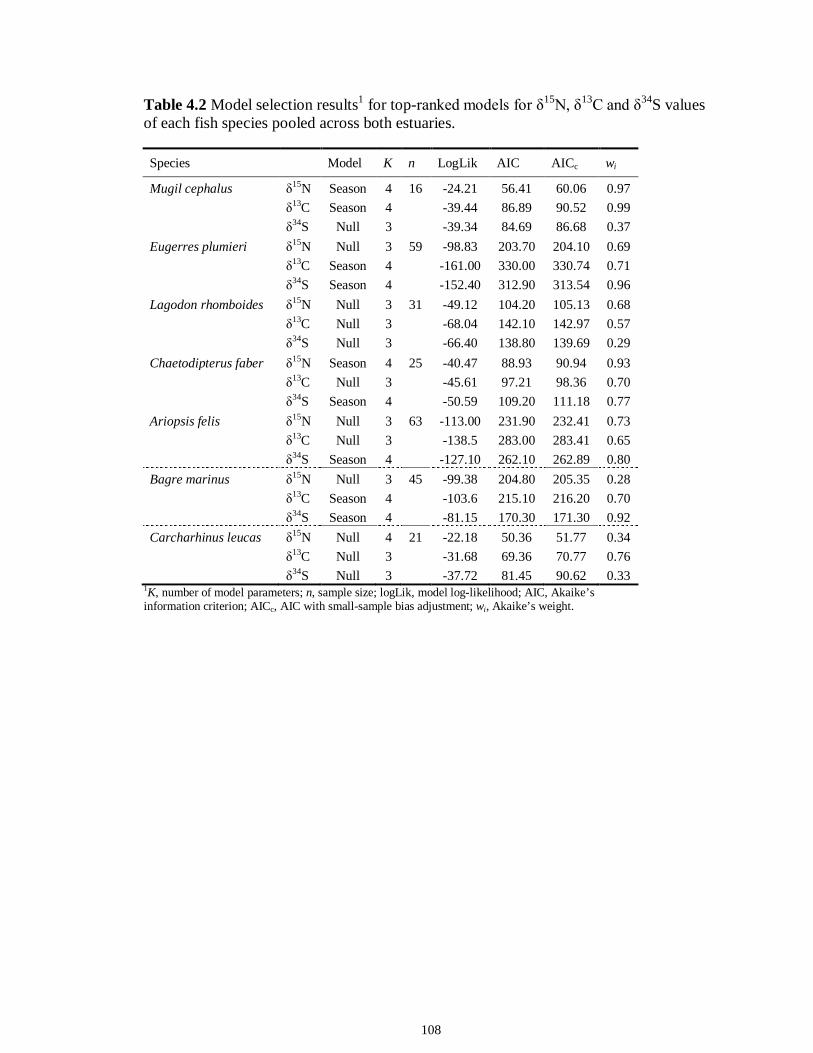
108

Table 4.2 Model selection results1 for top-ranked models for δ15N, δ13C and δ34S values of each fish species pooled across both estuaries.

Species Model K n LogLik AIC AICc wi

Mugil cephalus δ15N Season 4 16 -24.21 56.41 60.06 0.97 δ13C Season 4 -39.44 86.89 90.52 0.99 δ34S Null 3 -39.34 84.69 86.68 0.37 Eugerres plumieri δ15N Null 3 59 -98.83 203.70 204.10 0.69 δ13C Season 4 -161.00 330.00 330.74 0.71 δ34S Season 4 -152.40 312.90 313.54 0.96 Lagodon rhomboides δ15N Null 3 31 -49.12 104.20 105.13 0.68 δ13C Null 3 -68.04 142.10 142.97 0.57 δ34S Null 3 -66.40 138.80 139.69 0.29 Chaetodipterus faber δ15N Season 4 25 -40.47 88.93 90.94 0.93 δ13C Null 3 -45.61 97.21 98.36 0.70 δ34S Season 4 -50.59 109.20 111.18 0.77 Ariopsis felis δ15N Null 3 63 -113.00 231.90 232.41 0.73 δ13C Null 3 -138.5 283.00 283.41 0.65 δ34S Season 4 -127.10 262.10 262.89 0.80 Bagre marinus δ15N Null 3 45 -99.38 204.80 205.35 0.28 δ13C Season 4 -103.6 215.10 216.20 0.70 δ34S Season 4 -81.15 170.30 171.30 0.92 Carcharhinus leucas δ15N Null 4 21 -22.18 50.36 51.77 0.34 δ13C Null 3 -31.68 69.36 70.77 0.76 δ34S Null 3 -37.72 81.45 90.62 0.33

1K, number of model parameters; n, sample size; logLik, model log-likelihood; AIC, Akaike’s information criterion; AICc, AIC with small-sample bias adjustment; wi, Akaike’s weight.

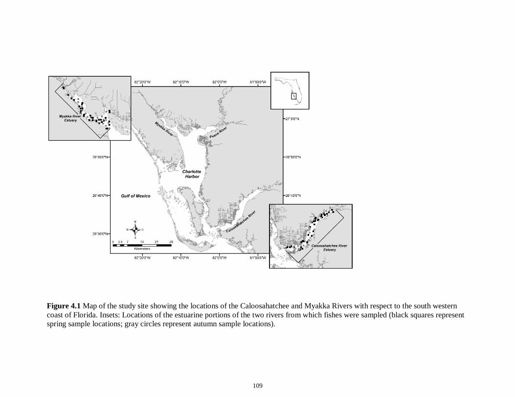
109

Figure 4.1 Map of the study site showing the locations of the Caloosahatchee and Myakka Rivers with respect to the south western coast of Florida. Insets: Locations of the estuarine portions of the two rivers from which fishes were sampled (black squares represent spring sample locations; gray circles represent autumn sample locations).

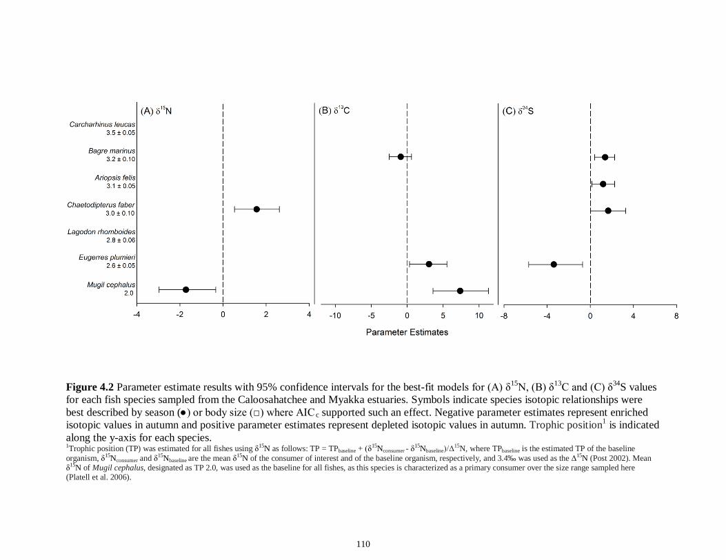
110

Figure 4.2 Parameter estimate results with 95% confidence intervals for the best-fit models for (A) δ15N, (B) δ13C and (C) δ34S values for each fish species sampled from the Caloosahatchee and Myakka estuaries. Symbols indicate species isotopic relationships were best described by season (●) or body size (□) where AIC c supported such an effect. Negative parameter estimates represent enriched isotopic values in autumn and positive parameter estimates represent depleted isotopic values in autumn. Trophic position1 is indicated along the y-axis for each species. 1Trophic position (TP) was estimated for all fishes using δ15N as follows: TP = TPbaseline + (δ15Nconsumer - δ15Nbaseline)/Δ15N, where TPbaseline is the estimated TP of the baseline organism, δ15Nconsumer and δ15Nbaseline are the mean δ15N of the consumer of interest and of the baseline organism, respectively, and 3.4‰ was used as the Δ15N (Post 2002). Mean δ15N of Mugil cephalus, designated as TP 2.0, was used as the baseline for all fishes, as this species is characterized as a primary consumer over the size range sampled here (Platell et al. 2006).

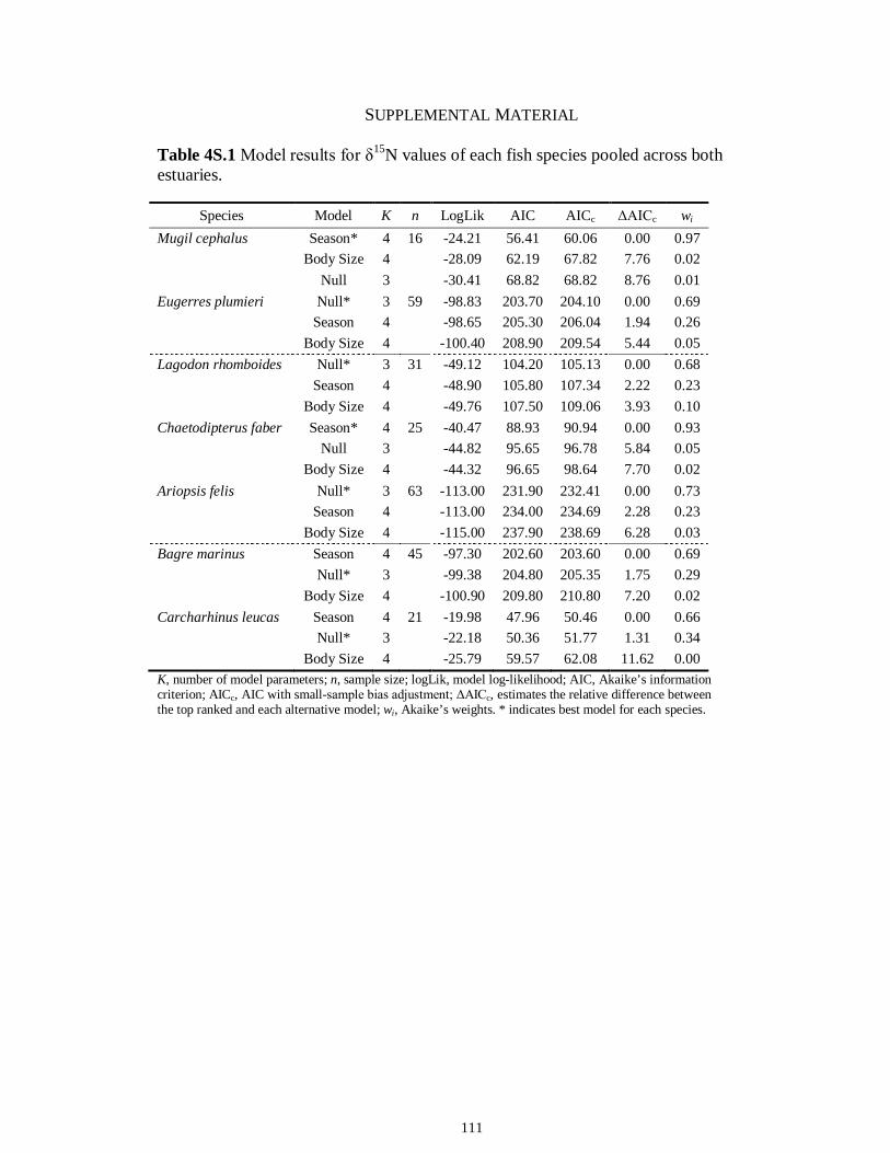
111

SUPPLEMENTAL MATERIAL

Table 4S.1 Model results for δ15N values of each fish species pooled across both estuaries.

Species Model K n LogLik AIC AICc ΔAICc wi Mugil cephalus Season* 4 16 -24.21 56.41 60.06 0.00 0.97 Body Size 4 -28.09 62.19 67.82 7.76 0.02 Null 3 -30.41 68.82 68.82 8.76 0.01 Eugerres plumieri Null* 3 59 -98.83 203.70 204.10 0.00 0.69 Season 4 -98.65 205.30 206.04 1.94 0.26 Body Size 4 -100.40 208.90 209.54 5.44 0.05 Lagodon rhomboides Null* 3 31 -49.12 104.20 105.13 0.00 0.68 Season 4 -48.90 105.80 107.34 2.22 0.23 Body Size 4 -49.76 107.50 109.06 3.93 0.10 Chaetodipterus faber Season* 4 25 -40.47 88.93 90.94 0.00 0.93 Null 3 -44.82 95.65 96.78 5.84 0.05 Body Size 4 -44.32 96.65 98.64 7.70 0.02 Ariopsis felis Null* 3 63 -113.00 231.90 232.41 0.00 0.73 Season 4 -113.00 234.00 234.69 2.28 0.23 Body Size 4 -115.00 237.90 238.69 6.28 0.03 Bagre marinus Season 4 45 -97.30 202.60 203.60 0.00 0.69 Null* 3 -99.38 204.80 205.35 1.75 0.29 Body Size 4 -100.90 209.80 210.80 7.20 0.02 Carcharhinus leucas Season 4 21 -19.98 47.96 50.46 0.00 0.66 Null* 3 -22.18 50.36 51.77 1.31 0.34 Body Size 4 -25.79 59.57 62.08 11.62 0.00 K, number of model parameters; n, sample size; logLik, model log-likelihood; AIC, Akaike’s information criterion; AICc, AIC with small-sample bias adjustment; ΔAICc, estimates the relative difference between the top ranked and each alternative model; wi, Akaike’s weights. * indicates best model for each species.

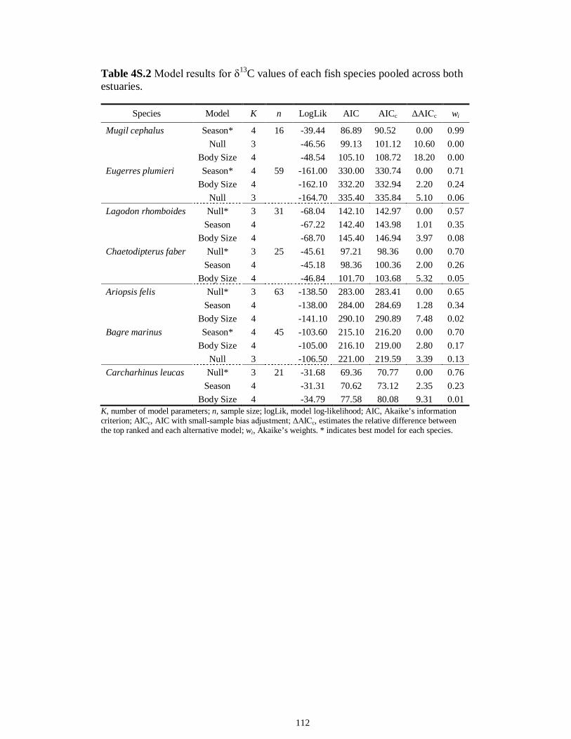
112

Table 4S.2 Model results for δ13C values of each fish species pooled across both estuaries.

Species Model K n LogLik AIC AICc ΔAICc wi

Mugil cephalus Season* 4 16 -39.44 86.89 90.52 0.00 0.99 Null 3 -46.56 99.13 101.12 10.60 0.00 Body Size 4 -48.54 105.10 108.72 18.20 0.00 Eugerres plumieri Season* 4 59 -161.00 330.00 330.74 0.00 0.71 Body Size 4 -162.10 332.20 332.94 2.20 0.24 Null 3 -164.70 335.40 335.84 5.10 0.06 Lagodon rhomboides Null* 3 31 -68.04 142.10 142.97 0.00 0.57 Season 4 -67.22 142.40 143.98 1.01 0.35 Body Size 4 -68.70 145.40 146.94 3.97 0.08 Chaetodipterus faber Null* 3 25 -45.61 97.21 98.36 0.00 0.70 Season 4 -45.18 98.36 100.36 2.00 0.26 Body Size 4 -46.84 101.70 103.68 5.32 0.05 Ariopsis felis Null* 3 63 -138.50 283.00 283.41 0.00 0.65 Season 4 -138.00 284.00 284.69 1.28 0.34 Body Size 4 -141.10 290.10 290.89 7.48 0.02 Bagre marinus Season* 4 45 -103.60 215.10 216.20 0.00 0.70 Body Size 4 -105.00 216.10 219.00 2.80 0.17 Null 3 -106.50 221.00 219.59 3.39 0.13 Carcharhinus leucas Null* 3 21 -31.68 69.36 70.77 0.00 0.76 Season 4 -31.31 70.62 73.12 2.35 0.23 Body Size 4 -34.79 77.58 80.08 9.31 0.01

K, number of model parameters; n, sample size; logLik, model log-likelihood; AIC, Akaike’s information criterion; AICc, AIC with small-sample bias adjustment; ΔAICc, estimates the relative difference between the top ranked and each alternative model; wi, Akaike’s weights. * indicates best model for each species.

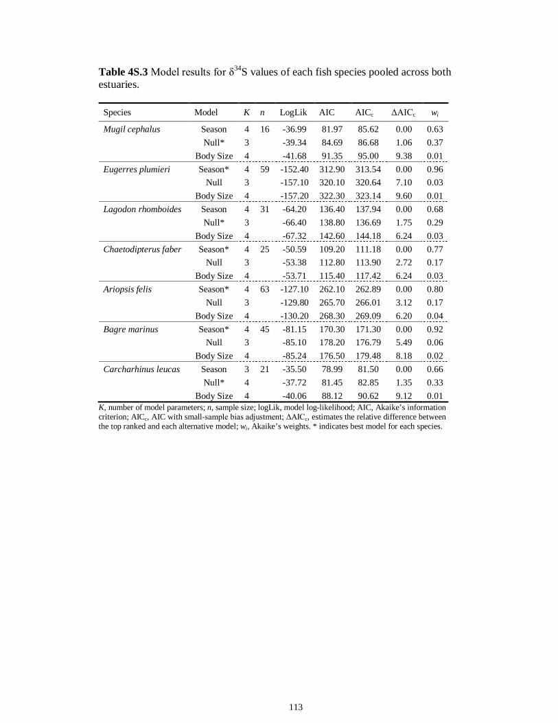
113

Table 4S.3 Model results for δ34S values of each fish species pooled across both estuaries.

Species Model K n LogLik AIC AICc ΔAICc wi

Mugil cephalus Season 4 16 -36.99 81.97 85.62 0.00 0.63 Null* 3 -39.34 84.69 86.68 1.06 0.37 Body Size 4 -41.68 91.35 95.00 9.38 0.01 Eugerres plumieri Season* 4 59 -152.40 312.90 313.54 0.00 0.96 Null 3 -157.10 320.10 320.64 7.10 0.03 Body Size 4 -157.20 322.30 323.14 9.60 0.01 Lagodon rhomboides Season 4 31 -64.20 136.40 137.94 0.00 0.68 Null* 3 -66.40 138.80 136.69 1.75 0.29 Body Size 4 -67.32 142.60 144.18 6.24 0.03 Chaetodipterus faber Season* 4 25 -50.59 109.20 111.18 0.00 0.77 Null 3 -53.38 112.80 113.90 2.72 0.17 Body Size 4 -53.71 115.40 117.42 6.24 0.03 Ariopsis felis Season* 4 63 -127.10 262.10 262.89 0.00 0.80 Null 3 -129.80 265.70 266.01 3.12 0.17 Body Size 4 -130.20 268.30 269.09 6.20 0.04 Bagre marinus Season* 4 45 -81.15 170.30 171.30 0.00 0.92 Null 3 -85.10 178.20 176.79 5.49 0.06 Body Size 4 -85.24 176.50 179.48 8.18 0.02 Carcharhinus leucas Season 3 21 -35.50 78.99 81.50 0.00 0.66 Null* 4 -37.72 81.45 82.85 1.35 0.33 Body Size 4 -40.06 88.12 90.62 9.12 0.01

K, number of model parameters; n, sample size; logLik, model log-likelihood; AIC, Akaike’s information criterion; AICc, AIC with small-sample bias adjustment; ΔAICc, estimates the relative difference between the top ranked and each alternative model; wi, Akaike’s weights. * indicates best model for each species.

114

CHAPTER 5

GOING WITH THE FLOW: SEASONAL SHIFTS IN THE FLOW OF ENERGY THROUGH

AN ESTUARINE FOOD WEB EXPERIENCING ALTERED HIGH FLOW

115

INTRODUCTION

Hydrological connectivity or the water-mediated transfer of matter, energy and/or

organisms within or between elements of the hydrological cycle, is considered to be the

most influential factor driving aquatic ecosystem dynamics (Pringle 2001).

Anthropogenic alterations to this connectivity, in the form of dams and diversions have

resulted in habitat fragmentation and degradation, and modifications to river flow

(Nilsson et al. 2005; Lotze et al. 2006). Modifications to river flow, primarily driven by

appropriation of freshwater for human use, is considered the most pervasive and

deleterious effect on rivers (Kingsford 2011). As few estuarine systems world-wide

remain unaffected by upstream manipulation of their freshwater inflow (Dynesius and

Nilsson 1994), these modifications can have major implications for individual species

and thus the structure of downstream estuarine and coastal marine communities (Edeline

et al. 2005; Serrano et al. 2010; Olin et al. in review).

The contribution of freshwater to downstream habitats is regarded as a critical

landscape process in riverine systems (Sklar and Browder 1998), regulating the physical,

chemical and biological properties of terrestrial, lacustrine, and marine environments

(Paerl et al. 2010; Rush et al. 2010). Within estuaries, freshwater inflow from riverine

sources provides nutrients, sediment and organic matter essential for primary and

secondary production (Mallin et al. 1993; Drinkwater and Frank 1994; Chanton and

Lewis 2002). Life history strategies (e.g., breeding, spawning and recruitment) of

estuarine species are commonly synchronized with particular flow patterns (Bunn and

Arthington 2002; Rehage and Trexler 2006) and variable salinity tolerances can produce

116

communities segregated along salinity gradients (Rakocinski et al. 1992; Gelwick et al.

2001; Montagna et al. 2002; Akin et al. 2003).

The occurrence of high freshwater flow events are considered a major form of

disturbance in riverine and estuarine systems and are often influential in restructuring

communities (Resh et al. 1988; Montagna et al. 2002), such as oyster reefs (e.g. Tolley et

al. 2006) and nekton assemblages (e.g. Olin et al. in review). Specifically, Olin et al. (in

review) demonstrated variable responses by nekton assemblages to natural and altered

flow patterns, whereby an increase in nekton density, diversity and species richness was

observed with the increase of flow in a natural estuary, whereas no changes in the same

metrics were observed in a flow-altered estuary. Thereby, suggesting a loss of seasonal

variability in these nekton assemblages with extreme high flows. This has broad

implications for individual species, in terms of their feeding ecology, trophic interactions

and dietary resource use, which in turn can impact ecological function and overall

stability of communities. From a community perspective, alterations to the estuarine

salinity gradient as a result of extreme high flows are anticipated to be most evident

among lower trophic level species (i.e., primary and secondary consumers). This

prediction is based on primary and secondary consumers having limited mobility, yet are

capable of assimilating variable mixtures of locally-based organic matter sources

(Deegan and Garritt 1997; Wainright et al. 2000; Hsieh et al. 2002), that often coincide

with changes in physiochemical processes (McLeod and Wing 2008).

The aim of this study was to test the hypothesis that estuarine food webs differ

between dry and wet seasons, and in so doing, specifically address the influence of

anthropogenically-induced high flow. Our objectives were to, (1) determine the effect of

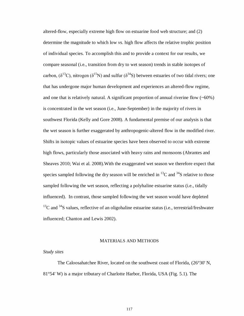
117

altered-flow, especially extreme high flow on estuarine food web structure; and (2)

determine the magnitude to which low vs. high flow affects the relative trophic position

of individual species. To accomplish this and to provide a context for our results, we

compare seasonal (i.e., transition from dry to wet season) trends in stable isotopes of

carbon, (δ13C), nitrogen (δ15N) and sulfur (δ34S) between estuaries of two tidal rivers; one

that has undergone major human development and experiences an altered-flow regime,

and one that is relatively natural. A significant proportion of annual riverine flow (~60%)

is concentrated in the wet season (i.e., June-September) in the majority of rivers in

southwest Florida (Kelly and Gore 2008). A fundamental premise of our analysis is that

the wet season is further exaggerated by anthropogenic-altered flow in the modified river.

Shifts in isotopic values of estuarine species have been observed to occur with extreme

high flows, particularly those associated with heavy rains and monsoons (Abrantes and

Sheaves 2010; Wai et al. 2008).With the exaggerated wet season we therefore expect that

species sampled following the dry season will be enriched in 13C and 34S relative to those

sampled following the wet season, reflecting a polyhaline estuarine status (i.e., tidally

influenced). In contrast, those sampled following the wet season would have depleted

13C and 34S values, reflective of an oligohaline estuarine status (i.e., terrestrial/freshwater

influenced; Chanton and Lewis 2002).

MATERIALS AND METHODS

Study sites

The Caloosahatchee River, located on the southwest coast of Florida, (26°30' N,

81°54' W) is a major tributary of Charlotte Harbor, Florida, USA (Fig. 5.1). The

118

Caloosahatchee River watershed drains an area of approximately 4,550 km2. Prior to the

artificial connection to Lake Okeechobee, the Caloosahatchee River was a smaller,

meandering river originating at the west end of Lake Flirt and extending to Beautiful

Island in Ft. Myers (Flaig and Capece 1998). Intensive agriculture became the major land

use in the watershed with the construction of extensive drainage projects in the 1880’s;

additional channelization and construction have occurred at Moore Haven (S-77), Ortona

(S-78) and Franklin Lock and Dam (S-79) (Flaig and Capece 1998). The Caloosahatchee

River currently extends about 68 km from Lake Okeechobee to S-79. This final

downstream structure defines the beginning of the Caloosahatchee Estuary and extends

for approximately 42 km to San Carlos Bay. These modifications to the hydrology of the

Caloosahatchee River in combination with land-use development (e.g., Ft. Myers) have

resulted in large-scale alterations in the estuary (Barnes 2005). The salinity gradient of

the Caloosahatchee estuary cycles annually; during the winter/spring months (dry season)

the estuary ranges from mesohaline (salinity ranging from 5 to 18‰) to polyhaline

(salinity range of 18 to 30‰) and during the summer/autumn months (wet season) the

estuary can become exclusively oligohaline (salinity range 0 to 5‰), with minimal tidal

influence (Fig. 5.2; Doering and Chamberlain 1998; Flaig and Capece 1998). This

transition between dry and wet seasons can be rapid, often occurring in less than a week

(Doering and Chamberlain 1998). After flows decrease, the river returns to a mesohaline

gradient.

The Myakka River (82°12' W, 26°57' N), draining into the northern portion of

Charlotte Harbor, was selected as a control site for comparison with the Caloosahatchee.

The Myakka River was chosen for several reasons; (1) it is proximately located (< 100

119

km; Fig. 5.1) to the Caloosahatchee River, and therefore is accessible by fishes and

macro-invertebrates of the Charlotte Harbor and; (2) in contrast to the Caloosahatchee

River, it experiences relatively natural flow periods and its shoreline areas have been

subjected to relatively minor anthropogenic modification. Further, although, much of the

shoreline habitat of the Caloosahatchee estuary has largely been altered by urbanization,

as evidenced by extensive shoreline modifications, the upper reaches and some

downstream areas are composed of similar ecological communities, including saltmarsh

and mangrove species. Specifically, the natural shoreline areas of both estuaries are

characterized by mangroves and saltmarsh, principally R. mangle, black mangrove

Avicennia germinans, saltmarsh cordgrass Spartina alterniflora and black needlerush

Juncus roemerianus. Palmer et al. (2011) and Vinagre et al. (2011) conducted

comparisons of community and food web structure of proximate estuaries respectively,

citing similar species composition among the two study systems. In this context, the

Myakka estuary provides a reference by which a comparison of food web dynamics to the

Caloosahatchee estuary can be made.

Sample collection

Samples were collected during 2008 targeting the dry (May and June) and wet

(September and October) seasons that occur in the Myakka and Caloosahatchee estuaries

(Fig. 5.2). In an effort to sample a broad range of nekton species (see Table 5.1 for a

complete list of species sampled), shallow water (< 10 m) longlines (800 m), seines (21.3

m with 3.2-mm stretch mesh, center bag), and trawls (6.1-m 3with 8-mm stretch mesh,

3.2-mm stretch mesh liner) were used for all collections. Longlines were set for periods

120

from 30 min to 2 h, with most set for approximately 1.5 h. The trawl was towed for 5–7

minutes at 0.6 m•s-1, providing a tow length of ~180 m. Trawl width averaged ~4 m,

providing an approximate area of 720 m2 sampled by a typical tow. The seine was

deployed from a boat in a shallow arc parallel to shore and hauled directly along the

shoreline. The two ends of the seine were pulled together, sampling an area of ~68 m2.

During each sampling event, environmental parameters—including temperature

(°C), salinity (ppt) and dissolved oxygen (mgl-1)—were recorded from depths ranging

from 0.5 to 2.5 m, using an YSI water quality meter (YSI Inc., Yellow Springs, OH,

USA; see Table 5S.1 Supplemental Material). Upon collection, all fishes and macro-

invertebrates were measured; standard length for fishes, carapace width for crabs and disc

width for stingrays (to the nearest mm). White muscle tissue was excised from the dorsal

area anterior to the first dorsal fin from all fishes and from the dorsal surface from

stingrays. Oysters and crabs were dissected prior to drying and only soft tissue was

retained for stable isotope analyses. Muscle tissue samples were stored on ice in the field

and then stored frozen upon return to the laboratory (-20° C).

Stable isotope analysis

Muscle tissues were sub-sampled (~1.0 g), freeze-dried for 48 h, and

homogenized in a SPEX CertiPrep 8000-D ball milling unit (SPEX CertiPrep, Metuchen,

New Jersey). Lipids are depleted in 13C relative to other major tissue components (i.e.,

proteins and carbohydrates; DeNiro and Epstein 1977) and their presence in muscle tissue

samples can negatively skew observed δ13C values (Post et al. 2007). To standardize δ13C

values within and among species, lipids were removed from all samples prior to isotopic

121

analysis using a modified method outlined by Bligh and Dyer (1959): twice vortexing the

pulverized tissue in 5 ml of 2:1 chloroform: methanol solution for 24 h and decanting the

solvent through filter paper to isolate the lipid-free study sample.

Relative abundances of nitrogen (15N/14N) and carbon (13C/12C) isotopes were

determined on ~0.5 mg sub-samples sealed in tin capsules on a Thermo Finnigan DeltaPlus

mass-spectrometer (Thermo Finnigan, San Jose, CA, USA) coupled with an elemental

analyzer (Costech, Valencia, CA, USA) at the Great Lakes Institute for Environmental

Research. Relative abundances of sulfur (34S/32S) were determined on ~2 mg and ~ 6 mg

sub-samples sealed in tin capsules on an Isochrom Continuous Flow IRMS (GV

Instruments / Micromass, UK) coupled with an elemental analyzer (Costech, Valencia,

CA, USA), at the Environmental Isotope Laboratory, University of Waterloo and by a

Thermo-Electron DeltaPlus Advantage IRMS at the Colorado Plateau Stable Isotope

Laboratory, Northern Arizona University, respectively.

Stable isotope results are expressed in standard delta notation (δ), defined as parts

per thousand as follows: δ = [(Rsample/Rstandard) -1] x 103 (Peterson and Fry 1987), where R

is the ratio of heavy to light isotopes in the sample and standard. The standard reference

material was atmospheric nitrogen for N2, Pee Dee Belemnite carbonate for CO2, and

Canyon Diablo Troilite for SO4. The analytical precision based on the standard deviation

of two standards (NIST 8414 and internal fish muscle lab standard; n = 76) for δ15N were

0.10‰ and 0.21‰ and for δ13C were 0.06‰ and 0.09‰, respectively, and based on three

sulfide standards (NBS-123, EIl-40 and EIL-43) for δ34S was 0.3‰. Analytical accuracy

based on the analysis of NIST standards, performed with muscle tissue sample, sucrose

(NIST 8542), ammonium sulfate (NIST 8547) and bovine liver and mussel samples (n =

122

3 for each), were within 0.07‰ for δ15N, 0.01‰ for δ13C, and 0.5‰ for δ34S, of certified

values.

Data analysis

To examine the effect of season (dry vs. wet) on the food webs of the Myakka (11

consumer species) and the Caloosahatchee estuaries (12 consumer species), analysis of

variance (ANOVA) was applied to the δ15N, δ13C and δ34S data of each species for each

estuary, separately. To further differentiate the food web response to altered flow, all

species were (1) assigned to one of four groups termed “trophic guilds” (see below) and

(2) to one of two groups termed “resource use categories” representing either pelagic or

benthic feeders. All assignments were based on dietary data from the literature (see Table

2 for designation). Trophic guilds were defined as: primary consumer, diet composed

largely of algae and detritus (>70%); secondary consumer, diet composed primarily of

invertebrate species; tertiary consumer, diet composed of both fishes and invertebrates

and; piscivore, diet composed primarily of fishes (> 80%). To examine the influence of

altered high-flow, resource use and their interaction on the defined trophic guilds, a two-

factor ANOVA was applied to the δ15N, δ13C and δ34S data of the secondary and tertiary

consumers in the Myakka, and the primary and secondary consumers in the

Caloosahatchee, as those trophic guilds included both pelagic and benthic feeders.

Prior to all analyses, stable isotope data were tested for normality using Shapiro-

Wilks test and for homogeneity of variance using Bartlett’s test. Isotope data were log

transformed to meet assumptions. All analyses were conducted in R 2.13.0 (R

123

Development Core Team 2011) with a criterion for significance of P < 0.05 used for all

statistical tests.

RESULTS

For the Myakka, the natural system, a similar range and magnitude of stable

isotope values of δ13C in the dry and wet seasons, respectively [(absolute range: 10.5‰

(range: -14.6 to -25.1) vs. 11.8‰ (range: -14.1 to -25.9)] and of δ15N [7.6‰ (range: 5.7 to

13.3) vs. 6.6‰ (range: 6.5 to 13.1)] was observed (Fig. 5.3). The range in δ34S values,

however, differed between dry and wet seasons [9.6‰ (range: 5.2 to 14.8) vs. 7.3‰

(range: 7.3 to 14.7)]. Similarly, in the Caloosahatchee, the range and magnitude of stable

isotope values observed between seasons were comparable [(absolute range: 14.8‰

(range: -12.4 to -27.2) vs. 14.8‰ (range: -14.3 to -29.1) for δ13C; 9.6‰ (range: 4.5 to

14.1) vs. 8.3‰ (range: 6.1 to 14.4) for δ15N; 15.3‰ (range: -0.3 to 15.0) vs. 15.0‰

(range: 1.4 to 16.4) for δ34S, respectively (Fig. 5.4)]). However, in contrast to the

Myakka, a clear shift in the range of food web values was observed in the

Caloosahatchee; depletion in 13C and enrichment in 15N of ~2‰. For each isotope the

absolute range of values in the dry and wet seasons were greater in the Caloosahatchee

relative to the Myakka (Fig. 5.3, 5.4).

In the Caloosahatchee, changes to the species-level δ15N-, δ13C- and δ34S-season

relationships were predominantly driven by primary and secondary consumers (see Table

5S.2 Supplemental Material for ANOVA statistics). Species whose δ13C values varied

significantly between season were all depleted in 13C following the wet season (Fig.

5.5A). For species that did not exhibit a significant shift in δ13C, a declining trend in δ13C

124

values with the wet season was observed, with the exception of Crassostrea virginica and

Eugerres plumieri (Fig. 5.5A). The δ15N values of the majority of primary and secondary

consumers were significantly enriched in 15N following altered-high flow (i.e. Fig. 5.5B).

The δ15N values of the primary consumers, C. virginica and M. cephalus, significantly

increased by approximately 2‰ and 1.5‰, respectively between seasons (Fig. 5.5B).

Unlike the Myakka, the δ34S values of tertiary consumers of the Caloosahatchee did not

show an overall depletion in 34S. On the contrary, Lutjanus griseus exhibited an

enrichment in 34S following the wet season (Fig. 5.5C).

In contrast to the Caloosahatchee, species in the Myakka exhibited a mixed

response to the onset of the wet season, but overall significant shifts in isotope values

were limited to only a few species (Fig. 5.5D-F; see Table 5S.2 Supplemental Material

for ANOVA statistics). These differences were principally driven by tertiary consumers.

No overall trend of depletion or enrichment was identified for 13C (Fig. 5.5D) or 15N (Fig.

5.5E). However significant depletion in 34S was identified in the tertiary consumers,

Ariopsis felis, Bagre marinus, and Cynoscion arenarius in the wet season (Fig. 5.5F).

When considering the relationships between season and resource use of trophic

guilds, in the Myakka, both secondary and tertiary consumers exhibited significant

differences in δ34S between seasons (Table 5.3). The δ15N values varied significantly with

resource use category in the secondary consumers, and with the interaction in tertiary

consumers (Table 5.3). The δ13C values varied significantly with resource use in the

tertiary consumers (Table 5.3). Together these results support the idea that benthic and

pelagic species derive their energy from different components of the food web. In

contrast, in the Caloosahatchee, the δ13C and δ15N values varied significantly with

125

season, resource use category and in the case of δ13C the interaction for primary

consumers (i.e., C. virginica and M. cephalus; Table 5.3), indicating that altered-high

flow affects both pelagic and benthic components of the food web. For δ13C, this is

specifically driven by the depletion observed in M. cephalus, whereas for δ15N, both

primary consumers showed enriched values of ~1.5‰ in the wet season. However, no

δ13C or δ15N effects were observed in secondary consumers. Statistically significant

differences in δ34S were limited to resource use, but were identified in both the primary

and secondary consumer trophic guilds (Table 5.3).

DISCUSSION

As the extent of alterations to natural hydrological connectivity increases to

accommodate the growing human demand for water resources, understanding the effects

of freshwater flow alteration are crucial for management and sustainability of estuarine

systems worldwide. Our comparison of seasonal dynamics of nekton assemblages in two

tidal estuaries that experience vastly different flow patterns indicates that

anthropogenically altered-high flow results in changes to isotopic values of estuarine

species that are not evident in a natural system. In the Myakka estuary, where the

hydrology is more natural than in the Caloosahatchee, there were no clear seasonal

isotopic patterns, with the exception of more estuarine δ34S values of tertiary consumers

in the wet season. In the Caloosahatchee estuary, the results revealed a dichotomous

response by estuarine species to altered-high flow. Specifically primary and secondary

consumers exhibited a distinct shift in δ13C and δ15N, whereas evidence of a weaker

response among higher trophic level species was detected. This shift in δ15N values and

126

δ13C to a lesser extent of the primary consumers (i.e. Crassostrea virginica and Mugil

cephalus), suggests that altered-high flow affected both pelagic and benthic components

of this estuarine food web. Differences in the response of conspecifics in the

Caloosahatchee support the assertion that high freshwater flow differentially affects

organisms and could indicate that the variable responses may be related to species-

specific behaviour, size or life-history characteristics (Power et al. 1996).

Estuaries that are strongly influenced by hydrologic conditions have been

observed to reflect seasonal differences in their basal productivity (Kaldy et al. 2005).

Our hypothesis was that species sampled following the dry season would reflect tidal

influence (i.e., enriched values of 13C and 34S) relative to those species sampled following

the compounded wet season, which would reflect freshwater influences (i.e. depleted

values of 13C and 34S). Given the extreme high flow event, this hypothesis was supported

in the Caloosahatchee by the δ13C data and was particularly evident in lower trophic level

species. The observed trends are consistent with our expectations of assimilation by the

estuarine species of a 13C-depleted source following high flow. This variation may be

attributed to two effects: the increasing influence of terrestrial organic matter with

extreme high flow and/or the increasing influence of 13C-depleted dissolved inorganic

carbon (DIC) sourcing phytoplankton in waters with decreasing salinity (Chanton and

Lewis 2002). When considering the values for marine organic matter and carbon from

plants that use the C4 photosynthetic process, they are enriched in 13C (δ13C of marine

plants, -18 to -22‰; δ13C of C4 plants, -6 to -19‰) relative to carbon sourced from C3

plants and terrestrial sources (δ13C of C3 plants, -24 to -30‰) (Moncreiff and Sullivan

2001; Winemiller et al. 2007). Marine plankton (-22‰; Chanton and Lewis 1999) also

127

tends to be more enriched than riverine plankton (-28‰; Chanton and Lewis 1999).

While the δ13C values of the consumers sampled from the Caloosahatchee remain more

similar to the marine end of the spectrum even after the wet season, there is a distinct

shift in primary and secondary consumers toward the terrestrial end of the spectrum.

With known species that partition their feeding strategies and resource use

between benthic vs. pelagic food webs (Table 5.2), our data suggest that lower trophic

levels, despite feeding in the benthic or pelagic food web, appear to be assimilating a

similar carbon source in the wet season. Firstly, there was a distinct depletion in 13C in

primary and secondary consumers in the modified estuary with altered high flow.

Whether the shift to more depleted 13C is a result of higher phytoplankton productivity or

inputs of terrestrial organic matter remains to be understood. And, unlike data presented

by Chanton and Lewis (2002), there was a general absence of 34S depletion and minimal

differences in δ34S values of species between seasons in the Caloosahatchee. Likely,

these results were observed because the mixing dynamics of estuaries favor the dominant

seawater sulfate source; the contribution of marine sulfate overwhelms the signal of

riverine sulfur, even at a salinity of l% (Chanton and Lewis 1999). However, the two

species that generally feed on pelagic resources, C. virginica and Chaetodipterus faber,

showed a similar depletion in 34S following high flow, suggestive of a sulfate from a

freshwater source (Fry and Chumchal 2011).

Temporal and spatial variation in basal resource δ13C and δ15N contributes to

variation in the isotopic signatures of consumers (Vander Zanden and Rasmussen 1999;

Matthews and Mazumder 2003). Therefore, ecosystem changes, such as shifts in salinity

regime or availability of terrestrial organic matter are likely first evidenced in the diet of

128

primary consumers, such as bivalves. Because it is relatively long-lived and sedentary,

the oyster, C. virginica—a good indicator species for ecosystem alteration—can provide

an important link between terrestrial organic matter and higher trophic level consumers

(Riera and Richard 1996, 1997; Chanton and Lewis 2002; Wilson et al. 2010). The fact

that δ13C of C. virginica sampled from the Caloosahatchee did not shift between seasons

in this study, maintaining δ13C values of ~-23‰, suggests continued use of a plankton-

based organic matter; however, the depletion in 34S and enrichment in 15N of the muscle

tissue of C. virginica between seasons, provides further support of a freshwater/terrestrial

influence from the available water-column carbon. Moreover, the significant depletion in

13C of the lower trophic level species (i.e., M. cephalus, Callinectes sapidus and

Eucinostomus harengulus) also supports a shift to a depleted 13C source. Although C.

virginica was not sampled in the Myakka, the δ13C trend of the benthic primary consumer

M. cephalus is similar to conspecifics in the Caloosahatchee, suggesting that the wet

season does alter isotopic values of lower trophic level consumers. Regardless of whether

C. virginica in the Myakka does exhibit depletion in 13C, these trends are not propagated

to higher trophic levels in that system. The significant δ13C shifts in the Caloosahatchee

with high flow strongly supports the trend of increased terrestrial influence. However

stable isotope values of primary production and organic matter sources would be required

to confirm these conclusions.

Stable isotope ratios of nitrogen generally increased following altered-high flow

in the modified Caloosahatchee, most notably in the primary and secondary consumers.

This trend was not apparent in the natural Myakka Estuary. It is unlikely that variation in

body size contributes significantly to the observed differences in δ15N of conspecifics

129

between seasons as demonstrated by Olin et al. (in revision). As well, it is unlikely that

prey resources shifted with altered flow, as unlike the positive response observed in the

Myakka, neither density nor species richness of consumers changed between seasons in

the Caloosahatchee Estuary (Olin et al. in review). Rather, these differences likely

reflected high nutrient loads associated with freshwater inflow, similar to McClelland and

Valiela (1998) who demonstrated a strong link between proximity to urbanization and

elevated δ15N values in estuarine species. The Caloosahatchee River and downstream

estuary receive considerable urban and agricultural runoff (Flaig and Capece 1998).

Although the variable levels of enrichment in 15N were observed throughout the

community and may be interpreted as relatively minor in the higher trophic level species,

the increase in δ15N values is consistent with the decrease in values of δ13C. This further

supports the conclusion that altered-high flow influences the available production and

nutrient resources available to these consumers.

A critical assumption, however, is that the species we examined exhibited site

fidelity, i.e. that they were present long enough to acquire the dominant isotopic signal of

the system. In our study, the δ13C of all primary and secondary consumers that exhibited

significant temporal differences decreased to a similar value. This result, coupled with the

enrichment of 15N in the majority of primary and secondary consumers, supports the

contention that most species were not moving to alternative habitats and were likely

integrating similar production sources. Indeed, a number of studies have demonstrated

that estuarine consumer species exhibit site fidelity and their tissues reflect the organic

matter close to the areas in which they inhabit (Deegan and Garritt 1997; Guest and

Connolly 2004).

130

The magnitude of response of the upper trophic level species to extreme high flow

in the Caloosahatchee was less relative to the lower trophic level species, based on stable

isotope values. Specifically, the absence of significant isotopic changes in the upper

trophic levels indicates that the shifts evidenced in the isotopes of the lower trophic levels

were not observed throughout the food web. One explanation for this response difference

could be that these upper trophic level species, which are generally more mobile,

migrated out of the Caloosahatchee estuary during high flow and continued to feed on

resources with similar isotope values. However the species considered were sampled

within the estuary during both collection periods. Moreover, the δ13C and δ15N trends of

these species were similar to those observed in the lower trophic levels, suggesting that

movement to, and subsequent feeding in a different ecosystem is unlikely. Rather, it

could be argued that the absence of a significant change in the isotopic values in the

upper trophic levels of the Caloosahatchee may indicate that the duration of high

freshwater flow was too short to elicit a shift in the isotope values of these species. Given

these species are of relatively large body size when compared with the primary and

secondary consumers, there would likely be a delay in the transfer of the new isotope

values from the lower trophic levels to those of higher trophic levels as a result of (1)

variable muscle tissue turnover rates in higher trophic level species and/or (2) a lag

associated with movement of different isotopic values through the food web (e.g.,

Guelinckx et al. 2007; Jennings et al. 2008). This is not to suggest that the isotopic values

of higher trophic level species do not change in a similar fashion to lower trophic level

species, just that the time associated with the trophic transfer of isotopes is longer than

the duration of the disturbance. This has consequences for using stable isotopes to assess

131

trophic ecology of species that have isotope turnover times in sampled tissues that are

longer than disturbance events (i.e., events that alter isotope values at the base of the food

web). Sampling of high turnover tissues, for example blood plasma (Hobson and Clark

1992), could aid in clarifying effect of high flow disturbance events on higher trophic

level species. Likewise, the use of alternative chemical tracers, such as fatty acids, could

provide a complementary mechanism for identifying temporal changes in prey resources

to a consumer (Hebert et al. 2009), and understanding the physiological response of an

organism (Arts et al. 2001) to this category of disturbance.

Although specific conclusions about diet and resource use by higher trophic level

species under the different freshwater flow regimes cannot be made, these results

indicated that higher trophic levels species are not as influenced by the high-flow in the

Caloosahatchee when compared to lower trophic level species. Since the stable isotope

values of muscle tissue reflect diet assimilated over a specific time period, minimal

change in δ15N and δ13C of the higher trophic species residing in the Caloosahatchee

through both seasons, indicated that the body composition of these animals, reflect

resources assimilated during both hydrologic regimes. Importantly, it also suggests that

disturbance of this magnitude does not systematically affect the upper trophic level

species included here, based on stable isotopes. In contrast the tissues of the lower trophic

level species of the Caloosahatchee reflected resources assimilated during each of the

seasons.

It is important to note, that if this disturbance event in the Caloosahatchee was of

longer duration or occurred more frequently, for example as predicted by global climate

change models (Pearlstine et al. 2010), then this alteration of the salinity gradient may

132

have more serious consequences, particularly with respect to the physiological and

dietary requirements of these species (e.g., maintaining osmotic balance; Nordlie 2006).

Indeed, Olin et al. (in review) demonstrated a loss of diversity and richness of marine

migrant species sampled via trawl and seine with the wet season in the Caloosahatchee.

Jack et al. (2009) further demonstrated the consequences of prolonged low-salinity events

which resulted in alteration to the diet of the red rock lobster, Jasus edwardsii, to a less

preferable species. The authors attributed this diet shift to reductions in the abundance of

filter-feeding invertebrates, including oysters (Pollack et al. 2011) and infaunal clams and

mussels (Rutger and Wing 2006; Jack et al. 2009). It is therefore critical to understand

the effects of anthropogenic modifications to hydrology on food web dynamics, as

community structure may be compromised and simplified through extirpation of non-

tolerant species. To advance our understanding of the species- and food web-level effects

observed in this study will require future studies that focus on determining seasonal

trends in primary production and organic matter sources, as well as monitoring trophic

structure of food webs that experience varying flow management strategies, for example,

pulse-release.

Conclusions

Establishment of freshwater inflow criteria is becoming increasingly important

(e.g., Arthington et al. 2006) however, development of these criteria is dependent on

understanding the response of communities to altered freshwater flow. This study

highlights shifts in food web structure likely driven by resource use (i.e., production

source) that occur in consumers, predominantly lower trophic level species of estuarine

133

communities, faced with altered flow. Shifts in resource use by primary and secondary

consumers with flow, are supported by previous studies in modified systems (Jack et al.

2009; McLeod et al. 2010). Alteration to riverine flow indeed has implications for

estuarine community structure (Olin et al. in review) and as presented here, the flow of

energy to higher trophic levels through the food web. Whether these implications result in

advantageous (e.g., nutrients for production) or deleterious (e.g., cause mortality) effects

to estuarine species requires further research. However, the results of this study indicate

that the assemblage of lower trophic level species could be influenced to a greater extent.

Ultimately the frequency, intensity and duration of each disturbance dictates the

characteristics that control ecosystem recovery, but the legacy effects of disturbance can

leave a system more vulnerable to additional disturbances (Scheffer et al. 2001; Harris et

al. 2010). Estuaries serve as nursery, rearing and feeding grounds for a diverse

assemblage of fish and invertebrate species (e.g. Beck et al. 2001) that are often of

recreational and commercial value. Thus, changes to natural flow regimes or anticipated

precipitation patterns that modify the duration and intensity of freshwater flow, may hold

significant consequences for the productivity of estuarine communities.

REFERENCES

Abrantes K.G. & Sheaves M. 2010. Importance of freshwater flow in terrestrial-aquatic energetic connectivity in intermittently connected estuaries of tropical Australia. Marine Biology 157:2071–2086. Adams A.J., Wolfe R.K. & Layman C.A. 2009. Preliminary examination of how human-driven freshwater flow alteration affects trophic ecology of juvenile snook (Centropomus undecimalis) in estuarine creeks. Estuaries and Coasts 32:819–828. Akin S., Winemiller K.O. & Gelwick F.P. 2003. Seasonal and spatial variation in fish and macrocrustracean assemblage structure in Mad Island March estuary, Texas. Estuarine,

134

Coastal and Shelf Science 57:269–282. Arthington A.H., Bunn S.E., Poff N.L. & Naiman R.J. 2006. The challenges of providing environmental flow rules to sustain river ecosystems. Ecological Applications 16:1311–1318. Arts M.T., Ackman R.G. & Holub B.J. 2001. Essential fatty acids in aquatic ecosystems: a crucial link between diet and human health and evolution. Canadian Journal of Fisheries and Aquatic Sciences 58:122–137. Austin H. & Austin S. 1971. The feeding habits of some juvenile marine fishes from the mangroves in western Puerto Rico. Caribbean Journal of Science 11:171–178. Barnes T. 2005. Caloosahatchee Estuary conceptual ecological model. Wetlands 25:884–897. Beck M.W., Heck K.L., Able K.W., Childers D.L., Eggleston D.B., Gillanders B.M., Halpern B., Hays C.G., Hoshino K., Minello T.J., Orth R.J., Sheridan P.F. & Weinstein M.P. 2001. The identification, conservation and management of estuarine and marine nurseries for fish and invertebrates. Bioscience 51:633–641. Bligh E.G. & Dyer W.J. 1959. A rapid method of total lipid extraction and purification. Canadian Journal of Physiology and Pharmacology 37:911–917. Bolnick D.I., Svanbäck R., Fordyce J.A., Yang L.H., Davis J.M., Hulsey C. & Forister M.L. 2003. The ecology of individuals: incidence and implications of individual specialization. American Naturalist 161:1–28. Bunn S.E. & Arthington A.H. 2002. Basic principles and ecological consequences of altered flow regimes for aquatic biodiversity. Environmental Management 30:492–507. Chanton J. & Lewis F.G. 2002. Examination of coupling between primary and secondary production in a river-dominated estuary: Apalachicola Bay, Florida, USA. Limnology and Oceanography 47:683–697. Chanton J. & Lewis F.G. 1999. Plankton and dissolved inorganic carbon isotopic composition in a river-dominated estuary: Apalachicola Bay, Florida. Estuaries 22:575–583. Cook D.A. 1994. Temporal patterns of food habits of the Atlantic stingray, Dasyatis sabina (Lesueur, 1824), from the Banana River Lagoon, Florida. MS thesis, Florida Institute of Technology. 45pp. Cortés E. 1999. Standardized diet compositions and trophic levels of sharks. ICES Journal of Marine Science 56:707–717.

135

Deegan L.A. & Garritt R.H. 1997. Evidence for spatial variability in estuarine food webs. Marine Ecology Progress Series 147:31–47. DeNiro M.J. & Epstein S. 1977. Mechanism of carbon isotope fractionation associated with lipid synthesis. Science 197:261–263. Derrick P.A. & Kennedy V.S. 1997. Prey selection by the hogchoker, Trinectes maculatus (Pisces: Soleidae), along summer salinity gradients in Chesapeake Bay, USA. Marine Biology 129:699–711. Doering P.H. & Chamberlain R.H. 1998. Water quality in the Caloosahatchee Estuary, San Carlos Bay and Pine Island Sound. In: Proceedings of the Charlotte Harbor Public Conference and Technical Symposium, Technical Report No. 98-02, Charlotte Harbor National Estuary Program, Punta Gorda, FL, pp. 229–240. Drinkwater K.F. & Frank K.T. 1994. Effect of river regulation and diversion on marine fish and invertebrates. Aquatic Conservation-Marine and Freshwater Ecosystems 4:135–151. Dynesius M. & Nilsson C. 1994. Fragmentation and flow regulation of river systems in the northern 3rd of the world. Science 266:753–762. Edeline E., Dufour S. & Elie P. 2005. Role of glass eel salinity preference in the control of habitat selection and growth plasticity in Anguilla anguilla. Marine Ecology Progress Series 304:191–199. Flaig E.G. & Capece J. 1998. Water use and runoff in the Caloosahatchee watershed. In: Proceedings of the Charlotte Harbor Public Conference and Technical Symposium, Technical Report No. 98-02, Charlotte Harbor National Estuary Program, Punta Gorda, FL, pp. 73–80. Fry B. & Chumchal M.M. 2011. Sulfur stable isotope indicators of residency in estuarine fish. Limnology and Oceanography 56:1563–1576. Gelwick F.P., Akin S., Arrington D.A. & Winemiller K.O. 2001. Fish assemblage structure in relation to environmental variation in a Texas Gulf coast wetland. Estuaries 24:285–296. Guelinckx J., Maes J., Van Den Driessche P., Geysen B., Dehairs F. & Ollevier F. 2007. Changes in δ13C and δ15N in different tissues of juvenile sand goby Pomatoschistus minutus: a laboratory diet-switch experiment. Marine Ecology Progress Series 341:205– 215. Guest M.A. & Connolly R.M. 2004. Fine-scale movement and assimilation of carbon in saltmarsh and mangrove habitat. Aquatic Ecology 38:599–609.

136

Harrigan P., Zieman J.C. & Macko S.A. 1989. The base of nutritional support for the gray snapper (Lutjanus griseus): an evaluation based on a combined stomach content and stable isotope analysis. Bulletin of Marine Science 44:65–77. Harris R.J., Milbrandt E.C., Everham E.M. & Bovard B.D. 2010. The effects of reduced tidal flushing on mangrove structure and function across a disturbance gradient. Estuaries and Coasts 33:1176–1185. Hayse J.W. 1990. Feeding habits, age, growth, and reproduction of Atlantic spadefish Chaetodipterus faber (Pisces: Ephippidae) in South Carolina. Fishery Bulletin 88:67– 83. Hebert C.E., Weseloh D.V.C., Gauthier L.T., Arts M.T. & Letcher R.J. 2009. Biochemical tracers reveal intra-specific differences in the food webs utilized by individual seabirds. Oecologia 160:15–23. Hobson K.A. & Clark R.G. 1992. Assessing avian diets using stable isotopes I: turnover of 13C in tissues. The Condor 94:181–188. Hsieh H.L., Chen C.P., Chen Y.G. & Yan H.H. 2002. Diversity of benthic organic matter flows through polychaetes and crabs in a mangrove estuary: δ13C and δ34S. Marine Ecology Progress Series 227:145–155. Idelberger C.F. & Greenwood M.F.D. 2005 Seasonal variation in fish assemblages within the estuarine portions of the Myakka and Peace Rivers, Southwest Florida. Gulf of Mexico Science 2:224–240. Jack L., Wing S.R. & McLeod R.J. 2009. Prey base shifts in red rock lobster Jasus edwardsii in response to habitat conversion in Fjordland marine reserves: implications for effective spatial management. Marine Ecology Progress Series 381:213–222. Jennings S., Maxwell T.A.D., Schratzberger M. & Milligan S.P. 2008. Body-size dependent temporal variation in nitrogen stable isotope ratios in food webs. Marine Ecology Progress Series 370:199–206. Kaldy J.E., Cifuentes L.A. & Brock D. 2005. Using stable isotope analyses to assess carbon dynamics in a shallow subtropical estuary. Estuaries 28:86–95. Kelly M.H. & Gore. 2008 J.A. Florida river flow patterns and the Atlantic multi-decadal oscillation. River Research and Applications 24:598–616. Kingsford R.T. 2011. Conservation management of rivers and wetlands under climate change –a synthesis. Marine and Freshwater Research 62:217–222. Laughlin R.A. 1982. Feeding habits of the blue crab, Callinectes sapidus (Rathbun), in the Apalachicola Estuary, Florida. Bulletin of Marine Science 32:807–822.

137

Layman C.A., Quattrochi J.P., Peyer C.M. & Allgeier J.E. 2007. Niche width collapse in a resilient top predator following ecosystem fragmentation. Ecology Letters 10:937–944. Ley J.A., Montague C.L. & McIvor C.C. 1994. Food habits of mangrove fishes: a comparison along estuarine gradients in northeastern Florida Bay. Bulletin of Marine Science 54:881–899. Lotze H.K., Lenihan H.S., Bourque B.J., Bradbury R.H., Cooke R.G., Kay M.C., Kidwell S.M., Kirby M.X., Peterson C.H. & Jackson J.B.C. 2006. Depletion, degradation, and recovery potential of estuaries and coastal seas. Science 312:1806–1809. Mallin M.A., Paerl H.W., Rudek J. & Bates P.W. 1993. Regulation of primary production by watershed rainfall and river flow. Marine Ecology Progress Series 93:199–203. Matthews B. & Mazumder A. 2003. Compositional and interlake variability of zooplankton affect baseline stable isotope signatures. Limnology and Oceanography 48:1977–1987. McClelland J.W. & Valiela I. 1998. Linking nitrogen in estuarine producers to land-derived sources. Limnology and Oceanography 43:577–585. McLeod R.J., Wing S.R. & Davis J.P. 2010. Habitat conversion and species loss alters the composition of carbon sources to benthic communities. Marine Ecology Progress Series 411:127–136. McLeod R.J. & Wing S.R. 2008. Influence of altered salinity regime on the population structure of two infaunal bivalve species. Estuarine, Coastal and Shelf Science 78:529–540. Moncreiff C.A. & Sullivan M.J. 2001. Trophic importance of epiphytic algae in subtropical seagrass beds: evidence from multiple stable isotope analyses. Marine Ecology Progress Series 215:93–106. Montagna P.A., Alber M., Doering P. & Connor M.S. 2002. Freshwater inflow: Science, policy, management. Estuaries 25:1243–1245. Motta P.J., Clifton K.B., Hernandez P., Eggold B.T., Giordano S.D. & Wilcox R. 1995. Feeding relationships among nine species of seagrass fishes of Tampa Bay, Florida. Bulletin of Marine Science 56:185–200. Nilsson C., Reidy C.A., Dynesius M. & Revenga C. 2005. Fragmentation and flow regulation of the world’s large river systems. Science 308:405–408. Nordlie F.G. 2006. Physiochemical environments and tolerances of cyprinodontoid fishes found in estuaries and salt marshes of eastern North America. Reviews in Fish Biology and Fisheries 16:51–106.

138

Olin J.A., Stevens P.W., Rush S.A., Hussey N.E. & Fisk A.T. Loss of seasonal variability in nekton community structure in a tidal river: evidence for homogenization in a flow-altered system. Ecological Applications In Review: 17 October 2011. Olin J.A., MacNeil M.A., Rush S.A. & Fisk A.T. Season-dominated variation in stable isotope ratios within fishes from two subtropical estuarine systems. Estuaries and Coasts In Revision: February 26, 2011. Olin J.A., Hussey N.E., Fritts M., Heupel M.R., Simpfendorfer C.A., Poulakis G.R. & Fisk A.T. 2011. Maternal meddling in neonatal sharks: implication for interpreting stable isotopes in young animals. Rapid Communications in Mass Spectrometry 25:1008–1016. Paerl H.W., Rossignol K.L., Hall S.N., Peierls B.L. & Wetz M.S. 2010. Phytoplankton community indicators of short- and long-term ecological change in the anthropogenically and climatically impacted Neuse River Estuary, North Carolina, USA. Estuaries and Coasts 33:485–497. Palmer T.A., Montagna P.A., Pollack J.B., Kalke R.D. & DeYoe H.R. 2011. The role of freshwater inflow in lagoons, rivers and bays. Hydrobiologia 667:49–67. Pearlstine L.G., Pearlstine E.V. & Aumen N.G. 2010. A review of the ecological consequence and management implications of climate change for the Everglades. Journal of the North American Benthological Society 29:1510–1526. Peterson B.J. & Fry B. 1987. Stable isotopes in ecosystem studies. Annual Review of Ecology and Systematics 18:293–320. Platell M.E., Orr P.A. & Potter I.C. 2006. Inter- and intraspecific partitioning of food resources by size large and abundant fish species in a seasonally open estuary. Journal of Fish Biology 69:243–262. Pollack J.B., Kim H.C., Morgan E.K. & Montagna P.A. 2011. Role of flood disturbance in natural oyster (Crassostrea virginica) population maintenance in an estuary in South Texas, USA. Estuaries and Coasts 34:187–197. Post D.M., Layman C.A., Arrington D.A., Takimoto G., Quattrochi J. & Montaña C.G. 2007. Getting to the fat of the matter: models, methods and assumptions for dealing with lipids in stable isotope analyses. Oecologia 152:179–189. Power M.E., Dietrich W.E. & Finlay J.C. 1996. Dams and downstream aquatic biodiversity: potential food web consequences of hydrologic and geomorphic change. Environmental Management 20:887–895. Pringle C.M. 2001. Hydrologic connectivity and the management of biological reserves: A global perspective. Ecological Applications 11:981–998.

139

Rakocinski C.F., Baltz D.M. & Fleeger J.W. 1992. Correspondence between environmental gradients and the community structure of marsh-edge fishes in a Louisiana estuary. Marine Ecology Progress Series 80:135–148. R Development Core Team. 2009. R: A language and environment for statistical computing. R Foundation for Statistical Computing, Vienna, Austria. Rehage J.S. & Trexler J.C. 2006. Assessing the net effect of anthropogenic disturbance on aquatic communities in wetlands: community structure relative to distance from canals. Hydrobiologia 569:359–373. Resh V.H., Brown A.V., Covich A.P., Gurtz M.E., Li H.W., Minshall G.W., Reice S.R., Sheldon A.L., Wallace J.B. & Wissmar R.C. 1988. The role of disturbance in stream ecology. Journal of the North American Benthological Society 7:433–455. Riera, P. & Richard P. 1997. Temporal variation of δ13C in particulate organic matter and oyster Crassostrea gigas in Marennes-Oléron Bay (France): Effect of freshwater inflow. Marine Ecology Progress Series 147:105–115. Riera P. & Richard P. 1996. Isotopic determination of food sources of Crassostrea gigas along a trophic gradient in the estuarine bay of Marennes-Oléron. Estuarine, Coastal and Shelf Science 42:347–360. Rush S.A., Olin J.A., Fisk A.T., Woodrey M.S. & Cooper R.J. 2010. Trophic relationships of a marsh bird differ between Gulf coast estuaries. Estuaries and Coasts 33:963–970. Rutger S.M. & Wing S.R. 2006. Effects of freshwater input on shallow-water infaunal communities in Doubtful Sound, New Zealand. Marine Ecology Progress Series 314:35–47. Scheffer M., Carpenter S., Foley J.A., Folke C. & Walker B. 2001. Catastrophic shifts in ecosystems. Nature 413:591–596. Serrano X., Grosell M. & Serafy J.E. 2010. Salinity selection and preference of the grey snapper Lutjanus griseus: field and laboratory observations. Journal of Fish Biology 76:1592–1608. Sheridan P.F., Trim D.L. & Baker B.M. 1984. Reproduction and food habits of seven species of Northern Gulf of Mexico fishes. Contributions in Marine Science 270:175–204. Sklar F.H. & Browder J.A. 1998. Coastal environmental impacts brought about by alterations to freshwater flow in the Gulf of Mexico. Environmental Management 22:547–562.

140

Tolley S.G., Volety A.K., Savarese M., Walls L.D., Lindardich C. & Everham E.M. 2006.Impacts of salinity and freshwater inflow on oyster-reef communities in Southwest Florida. Aquatic Living Resources 19:371–387. Vander Zanden M.J. & Rasmussen J.B. 1999. Primary consumer δ13C and δ15N and the trophic position of aquatic consumers. Ecology 80:1395–1404. Vinagre C., Saldago J., Cabral H.N. & Costa M.J. 2011. Food web structure and habitat connectivity in fish estuarine nurseries—impact of river flow. Estuaries and Coasts 34:663–674. Wai T.K., Ng J.S.S. & Leung K.M.Y. 2008. The source and fate of organic matter and the significance of detrital pathways in a tropical coastal ecosystem. Limnology and Oceanography 53:1479–1492. Wainright S.C., Weinstein M.P., Able K.W. & Currin C.A. 2000. Relative importance of benthic microalgae, phytoplankton and the detritus of smooth cordgrass Spartina alterniflora and the common reed Phragmites australis to brackish-marsh food webs. Marine Ecology Progress Series 200:77–91. Wilson R.M., Chanton J., Lewis F.G. & Nowacek D. 2010. Concentration-dependent stable isotope analysis of consumers in the upper reaches of a freshwater-dominated estuary: Apalachicola Bay, FL, USA. Estuaries and Coasts 33:1406–1419. Winemiller K.O., Akin S. & Zeug S.C. 2007. Production sources and food web structure of a temperate tidal estuary: integration of dietary and stable isotope data. Marine Ecology Progress Series 343:63–76. Woodland R.J., Secor D.H. & Wedge M.E. 2011. Trophic resource overlap between small elasmobranchs and sympatric teleosts in mid-Atlantic bight nearshore habitats. Estuaries and Coasts 34:391–404. Yáñez-Arancibia A. & Lara-Domínguez A.L. 1988. Ecology of three sea catfishes (Ariidae) in a tropical coastal ecosystem–Southern Gulf of Mexico. Marine Ecology Progress Series 49:215–230.

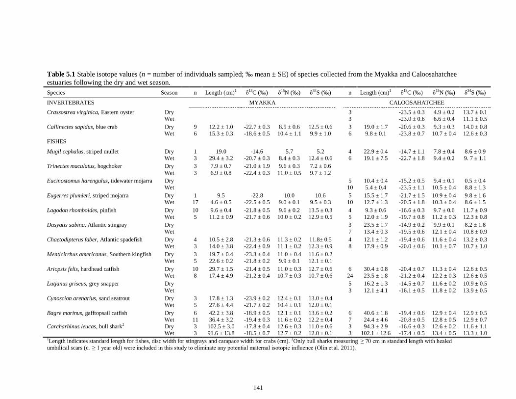
141

Table 5.1 Stable isotope values (n = number of individuals sampled; ‰ mean ± SE) of species collected from the Myakka and Caloosahatchee estuaries following the dry and wet season. Species Season n Length (cm)1 δ13C (‰) δ15N (‰) δ34S (‰) n Length (cm)1 δ13C (‰) δ15N (‰) δ34S (‰)

INVERTEBRATES MYAKKA CALOOSAHATCHEE Crassostrea virginica, Eastern oyster Dry 3 -23.5 ± 0.3 4.9 ± 0.2 13.7 ± 0.1 Wet 3 -23.0 ± 0.6 6.6 ± 0.4 11.1 ± 0.5 Callinectes sapidus, blue crab Dry 9 12.2 ± 1.0 -22.7 ± 0.3 8.5 ± 0.6 12.5 ± 0.6 3 19.0 ± 1.7 -20.6 ± 0.3 9.3 ± 0.3 14.0 ± 0.8 Wet 6 15.3 ± 0.3 -18.6 ± 0.5 10.4 ± 1.1 9.9 ± 1.0 6 9.8 ± 0.1 -23.8 ± 0.7 10.7 ± 0.4 12.6 ± 0.3 FISHES

Mugil cephalus, striped mullet Dry 1 19.0 -14.6 5.7 5.2 4 22.9 ± 0.4 -14.7 ± 1.1 7.8 ± 0.4 8.6 ± 0.9 Wet 3 29.4 ± 3.2 -20.7 ± 0.3 8.4 ± 0.3 12.4 ± 0.6 6 19.1 ± 7.5 -22.7 ± 1.8 9.4 ± 0.2 9. 7 ± 1.1 Trinectes maculatus, hogchoker Dry 3 7.9 ± 0.7 -21.0 ± 1.9 9.6 ± 0.3 7.2 ± 0.6 Wet 3 6.9 ± 0.8 -22.4 ± 0.3 11.0 ± 0.5 9.7 ± 1.2 Eucinostomus harengulus, tidewater mojarra Dry 5 10.4 ± 0.4 -15.2 ± 0.5 9.4 ± 0.1 0.5 ± 0.4 Wet 10 5.4 ± 0.4 -23.5 ± 1.1 10.5 ± 0.4 8.8 ± 1.3 Eugerres plumieri, striped mojarra Dry 1 9.5 -22.8 10.0 10.6 5 15.5 ± 1.7 -21.7 ± 1.5 10.9 ± 0.4 9.8 ± 1.6 Wet 17 4.6 ± 0.5 -22.5 ± 0.5 9.0 ± 0.1 9.5 ± 0.3 10 12.7 ± 1.3 -20.5 ± 1.8 10.3 ± 0.4 8.6 ± 1.5 Lagodon rhomboides, pinfish Dry 10 9.6 ± 0.4 -21.8 ± 0.5 9.6 ± 0.2 13.5 ± 0.3 4 9.3 ± 0.6 -16.6 ± 0.3 9.7 ± 0.6 11.7 ± 0.9 Wet 5 11.2 ± 0.9 -21.7 ± 0.6 10.0 ± 0.2 12.9 ± 0.5 5 12.0 ± 1.9 -19.7 ± 0.8 11.2 ± 0.3 12.3 ± 0.8 Dasyatis sabina, Atlantic stingray Dry 3 23.5 ± 1.7 -14.9 ± 0.2 9.9 ± 0.1 8.2 ± 1.8 Wet 7 13.4 ± 0.3 -19.5 ± 0.6 12.1 ± 0.4 10.8 ± 0.9 Chaetodipterus faber, Atlantic spadefish Dry 4 10.5 ± 2.8 -21.3 ± 0.6 11.3 ± 0.2 11.8± 0.5 4 12.1 ± 1.2 -19.4 ± 0.6 11.6 ± 0.4 13.2 ± 0.3 Wet 3 14.0 ± 3.8 -22.4 ± 0.9 11.1 ± 0.2 12.3 ± 0.9 8 17.9 ± 0.9 -20.0 ± 0.6 10.1 ± 0.7 10.7 ± 1.0 Menticirrhus americanus, Southern kingfish Dry 3 19.7 ± 0.4 -23.3 ± 0.4 11.0 ± 0.4 11.6 ± 0.2 Wet 5 22.6 ± 0.2 -21.8 ± 0.2 9.9 ± 0.1 12.1 ± 0.1 Ariopsis felis, hardhead catfish Dry 10 29.7 ± 1.5 -21.4 ± 0.5 11.0 ± 0.3 12.7 ± 0.6 6 30.4 ± 0.8 -20.4 ± 0.7 11.3 ± 0.4 12.6 ± 0.5 Wet 8 17.4 ± 4.9 -21.2 ± 0.4 10.7 ± 0.3 10.7 ± 0.6 24 23.5 ± 1.8 -21.2 ± 0.4 12.2 ± 0.3 12.6 ± 0.5 Lutjanus griseus, grey snapper Dry 5 16.2 ± 1.3 -14.5 ± 0.7 11.6 ± 0.2 10.9 ± 0.5 Wet 3 12.1 ± 4.1 -16.1 ± 0.5 11.8 ± 0.2 13.9 ± 0.5 Cynoscion arenarius, sand seatrout Dry 3 17.8 ± 1.3 -23.9 ± 0.2 12.4 ± 0.1 13.0 ± 0.4 Wet 5 27.6 ± 4.4 -21.7 ± 0.2 10.4 ± 0.1 12.0 ± 0.1 Bagre marinus, gafftopsail catfish Dry 6 42.2 ± 3.8 -18.9 ± 0.5 12.1 ± 0.1 13.6 ± 0.2 6 40.6 ± 1.8 -19.4 ± 0.6 12.9 ± 0.4 12.9 ± 0.5 Wet 11 36.4 ± 3.2 -19.4 ± 0.3 11.6 ± 0.2 12.2 ± 0.4 7 24.4 ± 4.6 -20.8 ± 0.5 12.8 ± 0.5 12.9 ± 0.7 Carcharhinus leucas, bull shark2 Dry 3 102.5 ± 3.0 -17.8 ± 0.4 12.6 ± 0.3 11.0 ± 0.6 3 94.3 ± 2.9 -16.6 ± 0.3 12.6 ± 0.2 11.6 ± 1.1 Wet 3 91.6 ± 13.8 -18.5 ± 0.7 12.7 ± 0.2 12.0 ± 0.1 3 102.1 ± 12.6 -17.4 ± 0.5 13.4 ± 0.5 13.3 ± 1.0 1Length indicates standard length for fishes, disc width for stingrays and carapace width for crabs (cm). 2Only bull sharks measuring ≥ 70 cm in standard length with healed umbilical scars (c. ≥ 1 year old) were included in this study to eliminate any potential maternal isotopic influence (Olin et al. 2011).

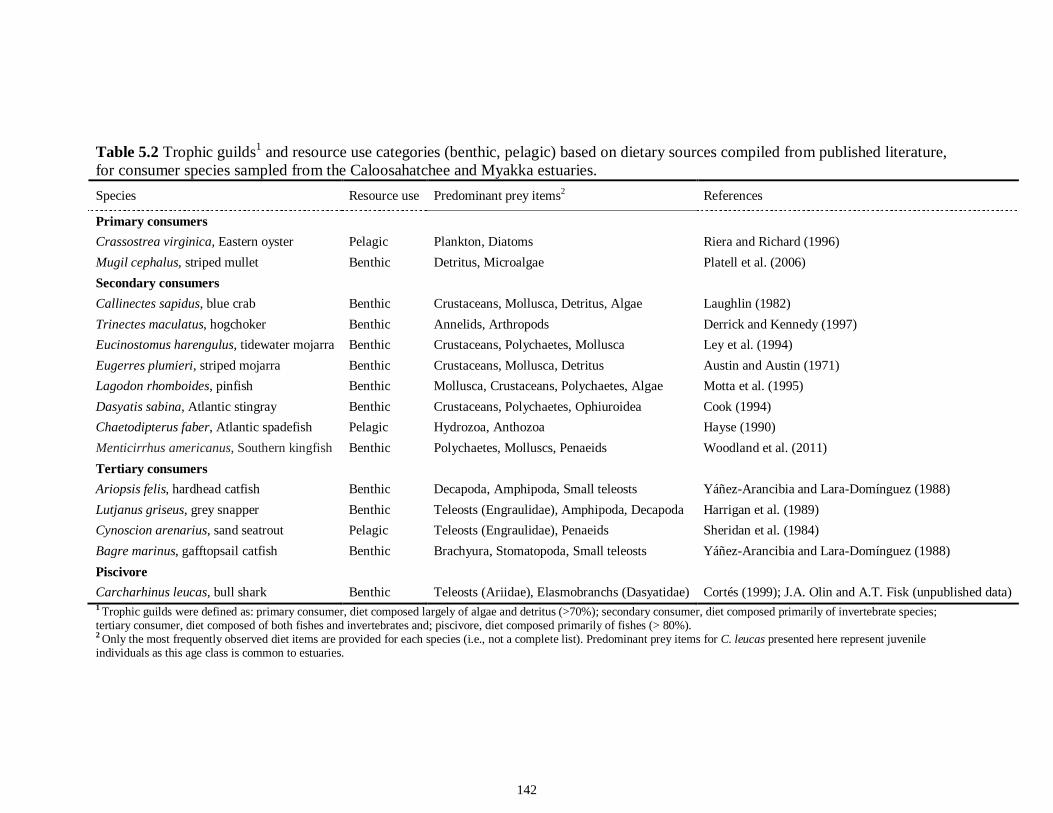
142

Table 5.2 Trophic guilds1 and resource use categories (benthic, pelagic) based on dietary sources compiled from published literature, for consumer species sampled from the Caloosahatchee and Myakka estuaries. Species Resource use Predominant prey items2 References

Primary consumers Crassostrea virginica, Eastern oyster Pelagic Plankton, Diatoms Riera and Richard (1996) Mugil cephalus, striped mullet Benthic Detritus, Microalgae Platell et al. (2006) Secondary consumers Callinectes sapidus, blue crab Benthic Crustaceans, Mollusca, Detritus, Algae Laughlin (1982) Trinectes maculatus, hogchoker Benthic Annelids, Arthropods Derrick and Kennedy (1997) Eucinostomus harengulus, tidewater mojarra Benthic Crustaceans, Polychaetes, Mollusca Ley et al. (1994) Eugerres plumieri, striped mojarra Benthic Crustaceans, Mollusca, Detritus Austin and Austin (1971) Lagodon rhomboides, pinfish Benthic Mollusca, Crustaceans, Polychaetes, Algae Motta et al. (1995) Dasyatis sabina, Atlantic stingray Benthic Crustaceans, Polychaetes, Ophiuroidea Cook (1994) Chaetodipterus faber, Atlantic spadefish Pelagic Hydrozoa, Anthozoa Hayse (1990) Menticirrhus americanus, Southern kingfish Benthic Polychaetes, Molluscs, Penaeids Woodland et al. (2011) Tertiary consumers Ariopsis felis, hardhead catfish Benthic Decapoda, Amphipoda, Small teleosts Yáñez-Arancibia and Lara-Domínguez (1988) Lutjanus griseus, grey snapper Benthic Teleosts (Engraulidae), Amphipoda, Decapoda Harrigan et al. (1989) Cynoscion arenarius, sand seatrout Pelagic Teleosts (Engraulidae), Penaeids Sheridan et al. (1984) Bagre marinus, gafftopsail catfish Benthic Brachyura, Stomatopoda, Small teleosts Yáñez-Arancibia and Lara-Domínguez (1988) Piscivore Carcharhinus leucas, bull shark Benthic Teleosts (Ariidae), Elasmobranchs (Dasyatidae) Cortés (1999); J.A. Olin and A.T. Fisk (unpublished data) 1 Trophic guilds were defined as: primary consumer, diet composed largely of algae and detritus (>70%); secondary consumer, diet composed primarily of invertebrate species; tertiary consumer, diet composed of both fishes and invertebrates and; piscivore, diet composed primarily of fishes (> 80%). 2 Only the most frequently observed diet items are provided for each species (i.e., not a complete list). Predominant prey items for C. leucas presented here represent juvenile individuals as this age class is common to estuaries.

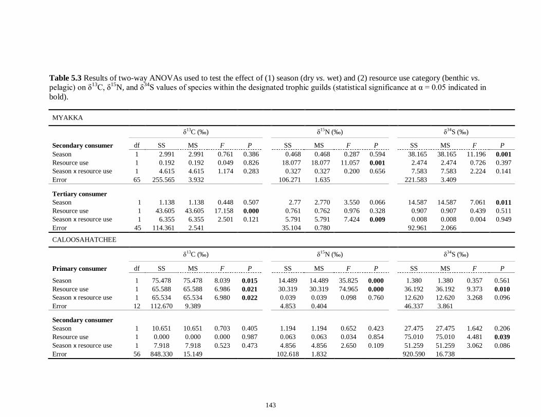
143

Table 5.3 Results of two-way ANOVAs used to test the effect of (1) season (dry vs. wet) and (2) resource use category (benthic vs. pelagic) on δ13C, δ15N, and δ34S values of species within the designated trophic guilds (statistical significance at α = 0.05 indicated in bold).

MYAKKA

δ13C (‰) δ15N (‰) δ34S (‰)

Secondary consumer df SS MS F P SS MS F P SS MS F P Season 1 2.991 2.991 0.761 0.386 0.468 0.468 0.287 0.594 38.165 38.165 11.196 0.001 Resource use 1 0.192 0.192 0.049 0.826 18.077 18.077 11.057 0.001 2.474 2.474 0.726 0.397 Season x resource use 1 4.615 4.615 1.174 0.283 0.327 0.327 0.200 0.656 7.583 7.583 2.224 0.141 Error 65 255.565 3.932 106.271 1.635 221.583 3.409

Tertiary consumer Season 1 1.138 1.138 0.448 0.507 2.77 2.770 3.550 0.066 14.587 14.587 7.061 0.011 Resource use 1 43.605 43.605 17.158 0.000 0.761 0.762 0.976 0.328 0.907 0.907 0.439 0.511 Season x resource use 1 6.355 6.355 2.501 0.121 5.791 5.791 7.424 0.009 0.008 0.008 0.004 0.949 Error 45 114.361 2.541 35.104 0.780 92.961 2.066

CALOOSAHATCHEE

δ13C (‰) δ15N (‰) δ34S (‰)

Primary consumer df SS MS F P SS MS F P SS MS F P

Season 1 75.478 75.478 8.039 0.015 14.489 14.489 35.825 0.000 1.380 1.380 0.357 0.561 Resource use 1 65.588 65.588 6.986 0.021 30.319 30.319 74.965 0.000 36.192 36.192 9.373 0.010 Season x resource use 1 65.534 65.534 6.980 0.022 0.039 0.039 0.098 0.760 12.620 12.620 3.268 0.096 Error 12 112.670 9.389 4.853 0.404 46.337 3.861

Secondary consumer Season 1 10.651 10.651 0.703 0.405 1.194 1.194 0.652 0.423 27.475 27.475 1.642 0.206 Resource use 1 0.000 0.000 0.000 0.987 0.063 0.063 0.034 0.854 75.010 75.010 4.481 0.039 Season x resource use 1 7.918 7.918 0.523 0.473 4.856 4.856 2.650 0.109 51.259 51.259 3.062 0.086 Error 56 848.330 15.149 102.618 1.832 920.590 16.738

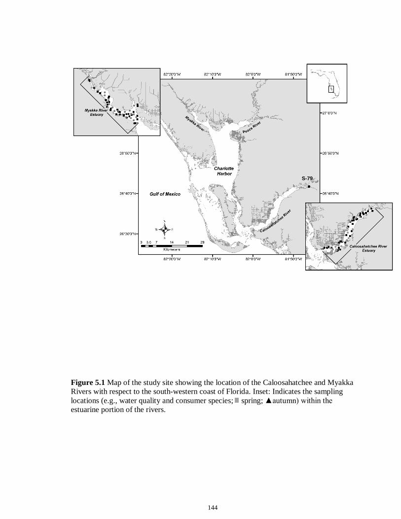
144

Figure 5.1 Map of the study site showing the location of the Caloosahatchee and Myakka Rivers with respect to the south-western coast of Florida. Inset: Indicates the sampling locations (e.g., water quality and consumer species; spring; ▲autumn) within the estuarine portion of the rivers.

S-79

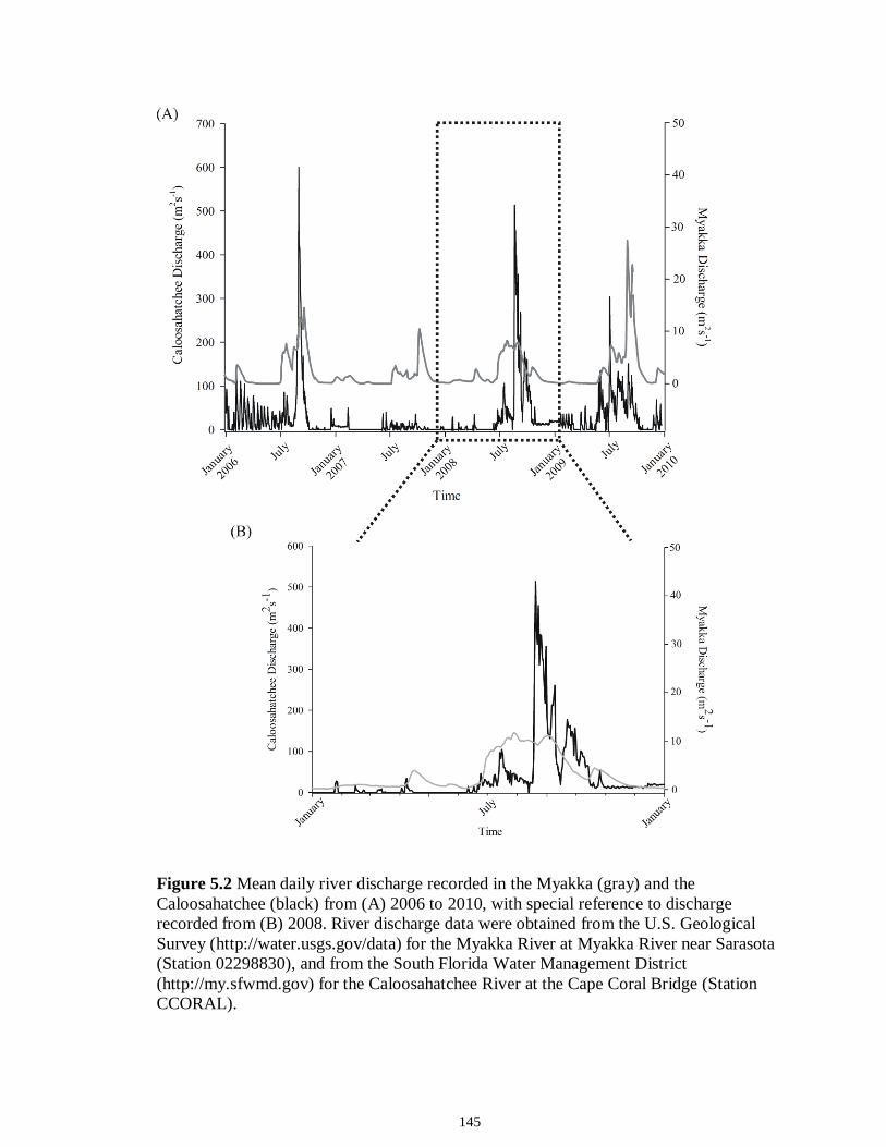
145

Figure 5.2 Mean daily river discharge recorded in the Myakka (gray) and the Caloosahatchee (black) from (A) 2006 to 2010, with special reference to discharge recorded from (B) 2008. River discharge data were obtained from the U.S. Geological Survey (http://water.usgs.gov/data) for the Myakka River at Myakka River near Sarasota (Station 02298830), and from the South Florida Water Management District (http://my.sfwmd.gov) for the Caloosahatchee River at the Cape Coral Bridge (Station CCORAL).

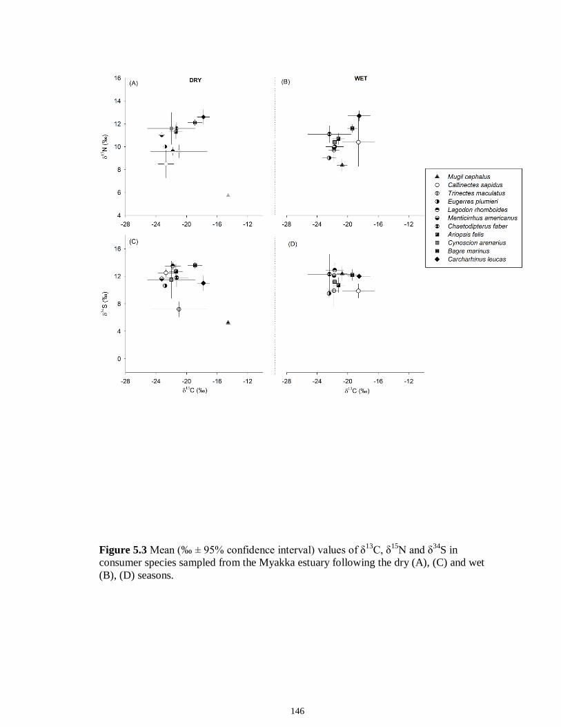
146

Figure 5.3 Mean (‰ ± 95% confidence interval) values of δ13C, δ15N and δ34S in consumer species sampled from the Myakka estuary following the dry (A), (C) and wet (B), (D) seasons.

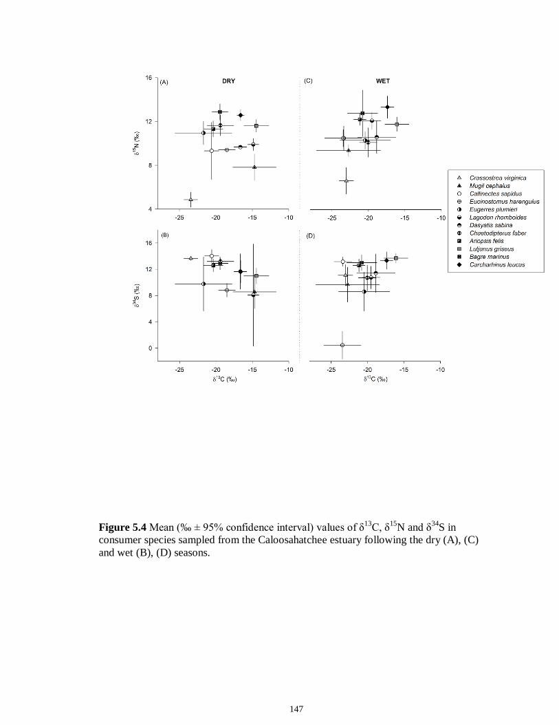
147

Figure 5.4 Mean (‰ ± 95% confidence interval) values of δ13C, δ15N and δ34S in consumer species sampled from the Caloosahatchee estuary following the dry (A), (C) and wet (B), (D) seasons.

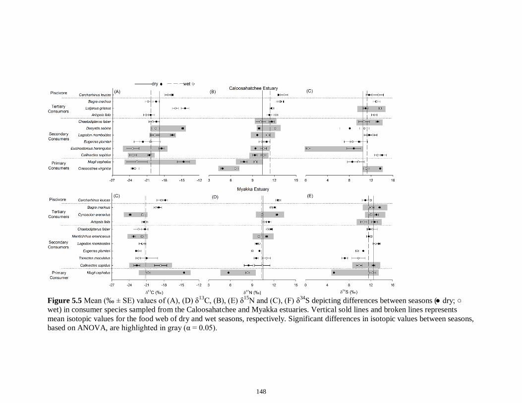
148

Figure 5.5 Mean (‰ ± SE) values of (A), (D) δ13C, (B), (E) δ15N and (C), (F) δ34S depicting differences between seasons (● dry; ○ wet) in consumer species sampled from the Caloosahatchee and Myakka estuaries. Vertical sold lines and broken lines represents mean isotopic values for the food web of dry and wet seasons, respectively. Significant differences in isotopic values between seasons, based on ANOVA, are highlighted in gray (α = 0.05).

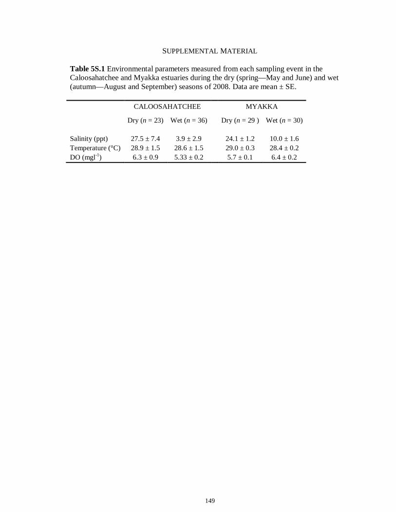
149

SUPPLEMENTAL MATERIAL

Table 5S.1 Environmental parameters measured from each sampling event in the Caloosahatchee and Myakka estuaries during the dry (spring—May and June) and wet (autumn—August and September) seasons of 2008. Data are mean ± SE.

CALOOSAHATCHEE MYAKKA

Dry (n = 23) Wet (n = 36) Dry (n = 29 ) Wet (n = 30) Salinity (ppt) 27.5 ± 7.4 3.9 ± 2.9 24.1 ± 1.2 10.0 ± 1.6 Temperature (°C) 28.9 ± 1.5 28.6 ± 1.5 29.0 ± 0.3 28.4 ± 0.2 DO (mgl-1) 6.3 ± 0.9 5.33 ± 0.2 5.7 ± 0.1 6.4 ± 0.2

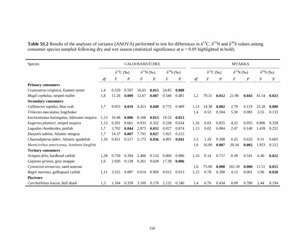
150

Table 5S.2 Results of the analyses of variance (ANOVA) performed to test for differences in δ13C, δ15N and δ34S values among consumer species sampled following dry and wet season (statistical significance at α = 0.05 highlighted in bold).

Species CALOOSAHATCHEE MYAKKA

δ13C (‰) δ15N (‰) δ34S (‰) δ13C (‰) δ15N (‰) δ34S (‰)

df F P F P F P df F P F P F P Primary consumers Crassostrea virginica, Eastern oyster 1,4 0.329 0.597 16.63 0.015 24.85 0.008 Mugil cephalus, striped mullet 1,8 11.26 0.009 12.67 0.007 0.546 0.481 1,2 79.31 0.012 21.96 0.043 41.54 0.023 Secondary consumers Callinectes sapidus, blue crab 1,7 9.053 0.019 4.413 0.040 0.772 0.409 1,13 14.38 0.002 2.79 0.119 23.28 0.000 Trinectes maculatus, hogchoker 1,4 0.53 0.504 5.30 0.083 3.55 0.133 Eucinostomus harengulus, tidewater mojarra 1,13 10.48 0.006 8.168 0.013 19.52 0.013 Eugerres plumieri, striped mojarra 1,13 0.201 0.661 0.933 0.352 0.238 0.634 1,16 0.03 0.855 4.32 0.055 0.896 0.358 Lagodon rhomboides, pinfish 1,7 3.702 0.044 2.875 0.032 0.027 0.874 1,13 0.02 0.884 2.47 0.140 1.439 0.252 Dasyatis sabina, Atlantic stingray 1,7 14.37 0.007 7.791 0.027 1.921 0.215 Chaetodipterus faber, Atlantic spadefish 1,10 0.451 0.517 5.173 0.036 4.891 0.041 1,5 1.29 0.308 0.25 0.633 0.31 0.602 Menticirrhus americanus, Southern kingfish 1,6 16.00 0.007 29.34 0.002 1.953 0.212 Tertiary consumers Ariopsis felis, hardhead catfish 1,28 0.750 0.394 2.406 0.132 0.000 0.986 1,16 0.14 0.717 0.39 0.541 6.40 0.022 Lutjanus griseus, grey snapper 1,6 2.926 0.138 0.261 0.628 17.38 0.006 Cynoscion arenarius, sand seatrout 1,6 75.00 0.000 161.30 0.000 11.51 0.015 Bagre marinus, gafftopsail catfish 1,11 3.515 0.087 0.014 0.909 0.012 0.913 1,15 0.78 0.398 4.12 0.061 5.96 0.028 Piscivore Carcharhinus leucas, bull shark 1,3 1.164 0.359 3.109 0.176 2.132 0.240 1,4 0.76 0.434 0.09 0.780 2.44 0.194

151

CHAPTER 6

CHANGES IN RESOURCE EXPLOITATION BY ESTUARINE CONSUMERS IN

RESPONSE TO ALTERED HIGH FLOW AS INFERRED FROM FATTY ACID

BIOMARKERS

152

INTRODUCTION

Production in tidal rivers represents a composite of a range of autochthonous and

allochthonous resources. Allochthonous contributions to these systems can include

terrestrially derived dissolved and/or particulate organic matter and leaf litter from

forested catchments and mangroves (Mfilinge et al. 2005; McLeod and Wing 2009).

Additionally, marine-derived organic matter from adjacent coastal habitats including

seagrass meadows and offshore planktonic production also contribute to the nutrient and

resource pools in estuarine food webs (Kharlamenko et al. 2001; Kang et al. 2003). It is

well established that this diverse range of resources is critical to the overall structure and

production of estuarine nekton communities (Chanton and Lewis 2002; Darnaude et al.

2005). However, barriers to this connectivity between the marine and terrestrial habitat

extremes of estuarine systems, such as altered hydrologic regimes, have the potential to

negatively impact the magnitude and timing of allochthonous contributions thereby

compromising biological productivity (Livingston et al. 1997; McLeod and Wing 2009;

Abrantes and Sheaves 2010).

The flow of energy and nutrients through food webs represents a complex

pathway of resource acquisition and assimilation from prey to predator species (Hobson

et al. 2002; Hebert et al. 2006). As such, many consumers have a high degree of feeding

plasticity, as the composition and availability of resources can vary both spatially and

temporally. Lipids typically represent the primary energy source in aquatic food webs

(Arts et al. 2009) and also provide critical fatty acid (FA) constituents that are required

for normal growth and development (Arts 1999). In this capacity, dietary FA have the

potential to provide insight toward the specific nutrient and energy resources exploited by

153

individual consumers (Dalsgaard et al. 2003). Specifically, essential fatty acids (EFA)

cannot be synthesized by many animal species and must therefore be obtained from the

diet in sufficient quantities to ensure optimal growth and development (Olsen 1999).

Central to their use as dietary tracers is the consideration that EFAs are also

minimally modified during their transfer from primary production to higher trophic level

consumers (Parrish et al. 2000; Dalsgaard and St. John 2004). Due to these

characteristics, FAs have been applied as natural diet biomarkers for a variety of

applications including understanding diet composition (Kharlamenko et al. 2001;

Bradshaw et al. 2003), changes in foraging strategies (Hebert et al. 2009), investigating

bottom-up primary production dynamics (Richoux and Froneman 2008; Koussoroplis et

al. 2011), and impacts of non-indigenous species introduction on nutrient transfer

(Nordin et al. 2008). Fatty acid biomarkers have been established/identified as

characteristic biomarkers of bacterial (Richoux and Froneman 2008), diatom,

dinoflagellate (Parrish et al. 2000), macroalgal (Johns et al .1979; Hanson et al. 2010) and

vascular plant production sources in a range of aquatic and terrestrial ecosystems

(Wannigama et al. 1981; Alfaro et al. 2006; Richoux and Froneman 2008). Such

specificity of individual FAs to primary production sources provides the potential to trace

the origin of organic matter in a system and to potentially resolve the differential

contributions of the range of autochthonous and allochthonous production sources in

dynamic systems such as tidal rivers. For example, aquatic primary production is

typically defined by greater proportions of ω3 polyunsaturated FA (PUFA) including

eicosapentaenoic acid (EPA; 20:5ω3), docosapentaenoic acid (DPA; 22:5ω3), and

docosahexaenoic acid (DHA; 22:6ω3). In contrast, terrestrial resources are commonly

154

characterized by increased contributions of ω6 PUFA such as linoleic acid (LIN;

18:2ω6), arachidonic acid (ARA; 20:4ω6) and γ-linolenic acid (18:3ω6; Smith et al.

2005; Koussoroplis et al. 2008).

Using the stable isotopes of carbon (δ13C), it was recently demonstrated that high

flow disturbance events may alter the general resource pathways exploited by primary

and secondary consumer species in an estuarine food web (Olin et al. unpublished data).

Indeed, Wai et al. (2008) demonstrated a shift in resource pathways of estuarine

invertebrates to a higher dependence on decomposing marine algae and terrestrial detritus

subsidies after an extreme tropical storm disturbance event. The authors further went on

to track these allochthonous trophic subsidies to higher order consumers, the bamboo

shark Chiloscyllium plagiosum (Wai et al. 2011). Given the influence of freshwater flow

in estuarine systems, the primary objective of the current study was to use FA biomarkers

to determine the main trophic pathways and relative importance of different energy

sources to estuarine consumers. To accomplish this objective, we compared seasonal FA

biomarker composition of estuarine nekton conspecifics from contrasting tidal rivers; one

that experiences regulated freshwater flow that often results in high flows, and one that

experiences more natural riverine flows. We hypothesized that the contribution of

allochthonous carbon sources (i.e., terrestrially-derived) would be more important during

the wet season than the dry season and would be especially evident during extreme high

flow. We expected that these differences will be manifest in reductions of ratios of ω3/ω6

indicating a greater contribution of terrestrial organic matter to production as opposed to

marine-based organic matter.

155

MATERIALS AND METHODS

Study sites, species and sample collection

We measured the concentrations of fatty acids in the total lipid fractions of

muscle tissue in estuarine consumers collected from the Caloosahatchee and Myakka

estuaries of southwest Florida. The Caloosahatchee River (26°30' N, 81°54' W) is part of

a cross-Florida canal system that passes through Lake Okeechobee and connects the

intracoastal waterways of Florida’s east and west coasts. The Caloosahatchee River has

been substantially altered over the past 100 yrs through the construction of an artificial

link to Lake Okeechobee, extensive canal systems, three locks to permit boat passage,

and dams to regulate water flow (Doering and Chamberlain 1998). These alterations to

the Rivers’ hydrology have greatly changed the freshwater flow in this system, resulting

in large fluctuations in timing and quantity of discharge to the estuarine portion of the

river (Flaig and Capece 1998; Barnes 2005). During periods of low freshwater discharge

(i.e., during winter/spring months), salt water regularly intrudes to S-79, the most

downstream water control structure, often exceeding 10‰ (see Fig. 2.1). High freshwater

discharge (i.e., during summer/fall months) can cause salinity to drop below 5‰ at the

mouth of the River and the transition between the two states can be rapid, sometimes

occurring in less than a week (Doering et al. 2002). The Myakka River (82°12' W, 26°57'

N) was chosen for comparison with the Caloosahatchee, as it is proximately located (<

100 km; Fig. 2.1) and therefore is accessible to fishes of Charlotte Harbor and

experiences similar temperature and weather patterns. More importantly, the Myakka

estuary has not been greatly modified by water control structure and experiences

156

relatively natural seasonal flow periods (for more detailed description of the estuaries, see

Olin et al. in review).

Species were collected following the dry (May and June) and wet (September and

October) seasons of 2008 from the Caloosahatchee and Myakka estuaries, using shallow

water (< 10 m) longlines (800 m), seines (21.3 m with 3.2-mm stretch mesh, center bag),

and trawls (6.1-m 3with 8-mm stretch mesh, 3.2-mm stretch mesh liner). Longlines were

set for periods from 30 min to 2 h, with most set for approximately 1.5 h. The seine was

deployed from a boat in a shallow arc parallel to shore and hauled directly along the

shoreline. The two ends of the seine were pulled together, sampling an area of ~68 m2.

The trawl was towed for 5–7 minutes at 0.6 m•s-1, providing a tow length of ~180 m.

Trawl width averaged ~4 m, providing an approximate area of 720 m2 sampled by a

typical tow.

For comparative purposes with previous studies that used stable isotopes to assess

altered high-flow affects on estuarine nekton consumers (Olin et al. unpublished data),

we selected six species representing different trophic guilds for FA analysis. These

species included (1) secondary consumers, blue crab Callinectes sapidus, pinfish

Lagodon rhomboides and Atlantic spadefish Chaetodipterus faber; (2) tertiary

consumers, hardhead catfish Ariopsis felis and gafftopsail catfish Bagre marinus and; (3)

a piscivore bull shark Carcharhinus leucas. Upon collection all species were measured;

carapace width for crabs and standard length for fishes (to the nearest mm). Crabs were

dissected prior to drying and only soft tissue was retained for analyses. White muscle

tissue was excised from the dorsal area anterior to the first dorsal fin from all fishes.

Muscle samples for fatty acid analysis were stored in a liquid nitrogen (LN2) dewar in the

157

field and then stored frozen in a cryogenic freezer upon return to the laboratory (-80ºC).

Only individuals of C. leucas with healed umbilical scars (c. ≥ 1 year old) were included

in this study to eliminate any potential influence from maternal resources (Olin et al.

2011; Belicka et al. unpublished data).

Lipid and fatty acid analysis

Fatty acid methyl esters (FAME) were obtained in a three-step process:

extraction, derivatization, and quantification on a gas chromatograph (GC). Briefly,

muscle tissues were sub-sampled and ~15–20 mg samples were extracted 3 times by

grinding freeze dried tissue in (2:1 vol:vol) chloroform:methanol (Bligh and Dyer 1959)

and centrifuged at 4,000 r.p.m. for 5 min to remove non-lipid material. A synthetic lipid

(cholestane) was added to all samples as an internal standard to provide an estimate of

extraction efficiency (Sigurgisladottir et al. 1992). From a final volume of 2 ml,

duplicate, 200 µL aliquots were dispensed into pre-weighed vessels which were dried and

re-weighed on a Sartorious M5 electron balance with 1 µg precision to provide a

quantitative measure of total lipid content. The remaining extract (1.6 ml) was then

transferred into a 5 ml Shimadzu vial (Sigma-Aldrich Canada Ltd, Oakville, CA) and

evaporated to dryness using nitrogen gas and stored at -80°C until derivatization. The

fatty acid extracts were re-suspended in 1.5 ml toluene prior to derivatization. Two

milliliters of H2SO4/methanol (1%) were added to the vial before overnight methylation

(16 h) in a water bath at 50°C. The extract was then evaporated to dryness under nitrogen,

and re-dissolved in 2 ml hexane and transferred to a 2 ml glass GC vial and stored in a -

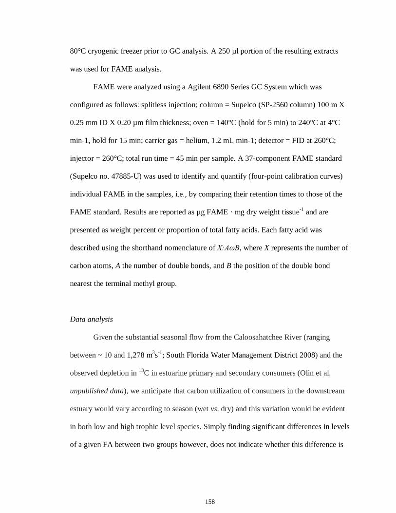
158

80°C cryogenic freezer prior to GC analysis. A 250 µl portion of the resulting extracts

was used for FAME analysis.

FAME were analyzed using a Agilent 6890 Series GC System which was

configured as follows: splitless injection; column = Supelco (SP-2560 column) 100 m X

0.25 mm ID X 0.20 µm film thickness; oven = 140°C (hold for 5 min) to 240°C at 4°C

min-1, hold for 15 min; carrier gas = helium, 1.2 mL min-1; detector = FID at 260°C;

injector = 260°C; total run time = 45 min per sample. A 37-component FAME standard

(Supelco no. 47885-U) was used to identify and quantify (four-point calibration curves)

individual FAME in the samples, i.e., by comparing their retention times to those of the

FAME standard. Results are reported as µg FAME · mg dry weight tissue-1 and are

presented as weight percent or proportion of total fatty acids. Each fatty acid was

described using the shorthand nomenclature of X:AωB, where X represents the number of

carbon atoms, A the number of double bonds, and B the position of the double bond

nearest the terminal methyl group.

Data analysis

Given the substantial seasonal flow from the Caloosahatchee River (ranging

between ~ 10 and 1,278 m3s-1; South Florida Water Management District 2008) and the

observed depletion in 13C in estuarine primary and secondary consumers (Olin et al.

unpublished data), we anticipate that carbon utilization of consumers in the downstream

estuary would vary according to season (wet vs. dry) and this variation would be evident

in both low and high trophic level species. Simply finding significant differences in levels

of a given FA between two groups however, does not indicate whether this difference is

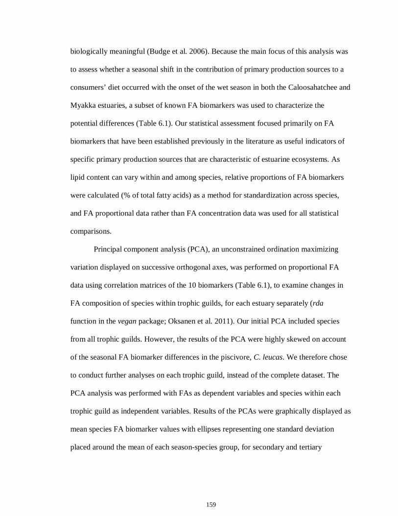
159

biologically meaningful (Budge et al. 2006). Because the main focus of this analysis was

to assess whether a seasonal shift in the contribution of primary production sources to a

consumers’ diet occurred with the onset of the wet season in both the Caloosahatchee and

Myakka estuaries, a subset of known FA biomarkers was used to characterize the

potential differences (Table 6.1). Our statistical assessment focused primarily on FA

biomarkers that have been established previously in the literature as useful indicators of

specific primary production sources that are characteristic of estuarine ecosystems. As

lipid content can vary within and among species, relative proportions of FA biomarkers

were calculated (% of total fatty acids) as a method for standardization across species,

and FA proportional data rather than FA concentration data was used for all statistical

comparisons.

Principal component analysis (PCA), an unconstrained ordination maximizing

variation displayed on successive orthogonal axes, was performed on proportional FA

data using correlation matrices of the 10 biomarkers (Table 6.1), to examine changes in

FA composition of species within trophic guilds, for each estuary separately (rda

function in the vegan package; Oksanen et al. 2011). Our initial PCA included species

from all trophic guilds. However, the results of the PCA were highly skewed on account

of the seasonal FA biomarker differences in the piscivore, C. leucas. We therefore chose

to conduct further analyses on each trophic guild, instead of the complete dataset. The

PCA analysis was performed with FAs as dependent variables and species within each

trophic guild as independent variables. Results of the PCAs were graphically displayed as

mean species FA biomarker values with ellipses representing one standard deviation

placed around the mean of each season-species group, for secondary and tertiary

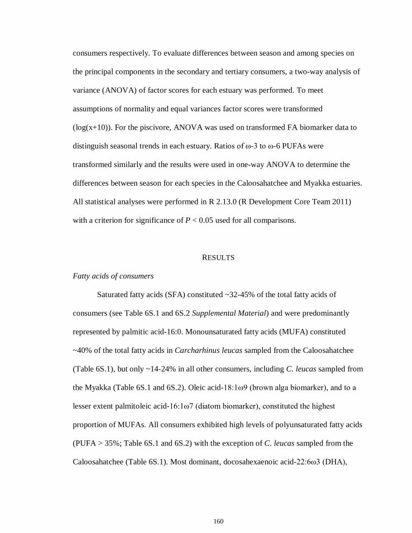
160

consumers respectively. To evaluate differences between season and among species on

the principal components in the secondary and tertiary consumers, a two-way analysis of

variance (ANOVA) of factor scores for each estuary was performed. To meet

assumptions of normality and equal variances factor scores were transformed

(log(x+10)). For the piscivore, ANOVA was used on transformed FA biomarker data to

distinguish seasonal trends in each estuary. Ratios of ω-3 to ω-6 PUFAs were

transformed similarly and the results were used in one-way ANOVA to determine the

differences between season for each species in the Caloosahatchee and Myakka estuaries.

All statistical analyses were performed in R 2.13.0 (R Development Core Team 2011)

with a criterion for significance of P < 0.05 used for all comparisons.

RESULTS

Fatty acids of consumers

Saturated fatty acids (SFA) constituted ~32-45% of the total fatty acids of

consumers (see Table 6S.1 and 6S.2 Supplemental Material) and were predominantly

represented by palmitic acid-16:0. Monounsaturated fatty acids (MUFA) constituted

~40% of the total fatty acids in Carcharhinus leucas sampled from the Caloosahatchee

(Table 6S.1), but only ~14-24% in all other consumers, including C. leucas sampled from

the Myakka (Table 6S.1 and 6S.2). Oleic acid-18:1ω9 (brown alga biomarker), and to a

lesser extent palmitoleic acid-16:1ω7 (diatom biomarker), constituted the highest

proportion of MUFAs. All consumers exhibited high levels of polyunsaturated fatty acids

(PUFA > 35%; Table 6S.1 and 6S.2) with the exception of C. leucas sampled from the

Caloosahatchee (Table 6S.1). Most dominant, docosahexaenoic acid-22:6ω3 (DHA),

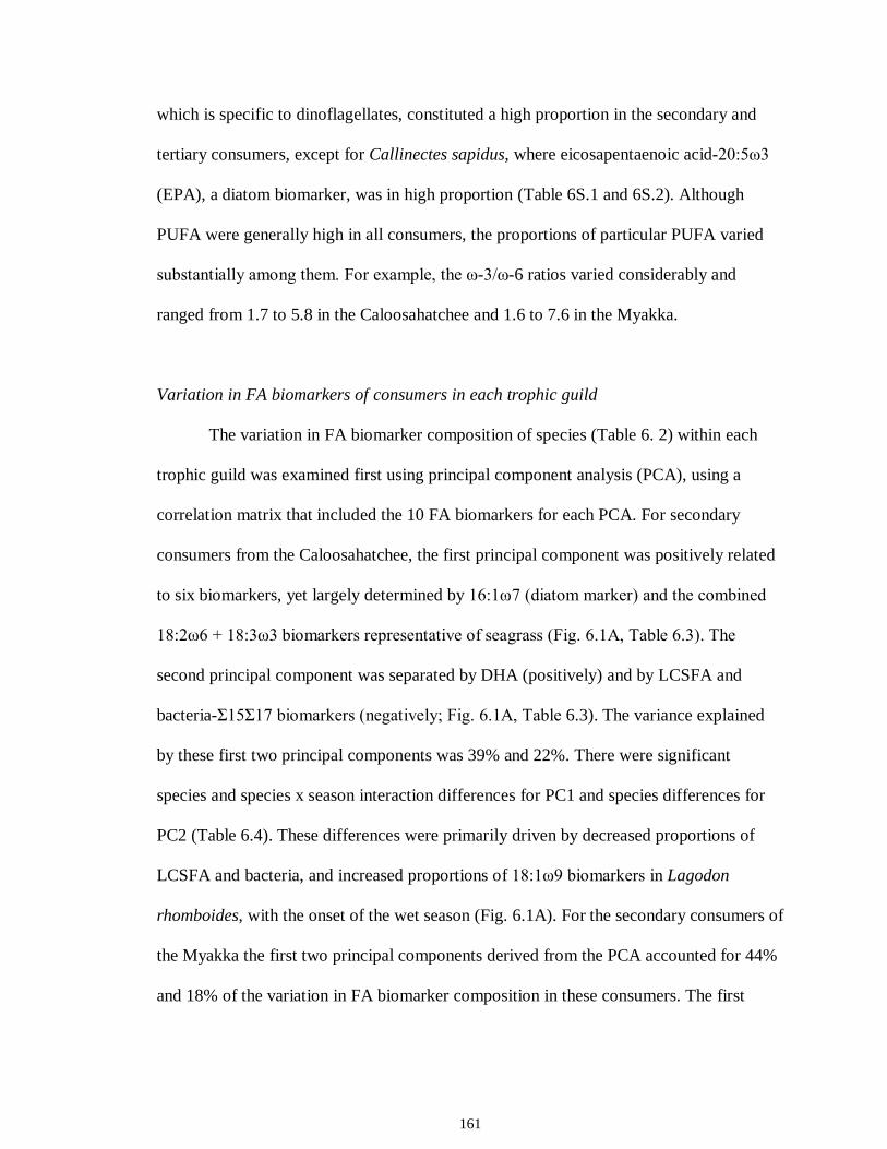
161

which is specific to dinoflagellates, constituted a high proportion in the secondary and

tertiary consumers, except for Callinectes sapidus, where eicosapentaenoic acid-20:5ω3

(EPA), a diatom biomarker, was in high proportion (Table 6S.1 and 6S.2). Although

PUFA were generally high in all consumers, the proportions of particular PUFA varied

substantially among them. For example, the ω-3/ω-6 ratios varied considerably and

ranged from 1.7 to 5.8 in the Caloosahatchee and 1.6 to 7.6 in the Myakka.

Variation in FA biomarkers of consumers in each trophic guild

The variation in FA biomarker composition of species (Table 6. 2) within each

trophic guild was examined first using principal component analysis (PCA), using a

correlation matrix that included the 10 FA biomarkers for each PCA. For secondary

consumers from the Caloosahatchee, the first principal component was positively related

to six biomarkers, yet largely determined by 16:1ω7 (diatom marker) and the combined

18:2ω6 + 18:3ω3 biomarkers representative of seagrass (Fig. 6.1A, Table 6.3). The

second principal component was separated by DHA (positively) and by LCSFA and

bacteria-Σ15Σ17 biomarkers (negatively; Fig. 6.1A, Table 6.3). The variance explained

by these first two principal components was 39% and 22%. There were significant

species and species x season interaction differences for PC1 and species differences for

PC2 (Table 6.4). These differences were primarily driven by decreased proportions of

LCSFA and bacteria, and increased proportions of 18:1ω9 biomarkers in Lagodon

rhomboides, with the onset of the wet season (Fig. 6.1A). For the secondary consumers of

the Myakka the first two principal components derived from the PCA accounted for 44%

and 18% of the variation in FA biomarker composition in these consumers. The first

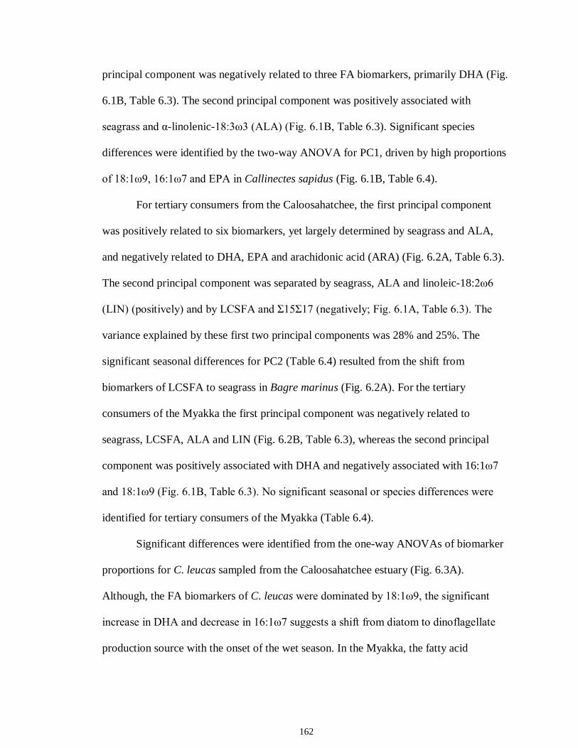
162

principal component was negatively related to three FA biomarkers, primarily DHA (Fig.

6.1B, Table 6.3). The second principal component was positively associated with

seagrass and α-linolenic-18:3ω3 (ALA) (Fig. 6.1B, Table 6.3). Significant species

differences were identified by the two-way ANOVA for PC1, driven by high proportions

of 18:1ω9, 16:1ω7 and EPA in Callinectes sapidus (Fig. 6.1B, Table 6.4).

For tertiary consumers from the Caloosahatchee, the first principal component

was positively related to six biomarkers, yet largely determined by seagrass and ALA,

and negatively related to DHA, EPA and arachidonic acid (ARA) (Fig. 6.2A, Table 6.3).

The second principal component was separated by seagrass, ALA and linoleic-18:2ω6

(LIN) (positively) and by LCSFA and Σ15Σ17 (negatively; Fig. 6.1A, Table 6.3). The

variance explained by these first two principal components was 28% and 25%. The

significant seasonal differences for PC2 (Table 6.4) resulted from the shift from

biomarkers of LCSFA to seagrass in Bagre marinus (Fig. 6.2A). For the tertiary

consumers of the Myakka the first principal component was negatively related to

seagrass, LCSFA, ALA and LIN (Fig. 6.2B, Table 6.3), whereas the second principal

component was positively associated with DHA and negatively associated with 16:1ω7

and 18:1ω9 (Fig. 6.1B, Table 6.3). No significant seasonal or species differences were

identified for tertiary consumers of the Myakka (Table 6.4).

Significant differences were identified from the one-way ANOVAs of biomarker

proportions for C. leucas sampled from the Caloosahatchee estuary (Fig. 6.3A).

Although, the FA biomarkers of C. leucas were dominated by 18:1ω9, the significant

increase in DHA and decrease in 16:1ω7 suggests a shift from diatom to dinoflagellate

production source with the onset of the wet season. In the Myakka, the fatty acid

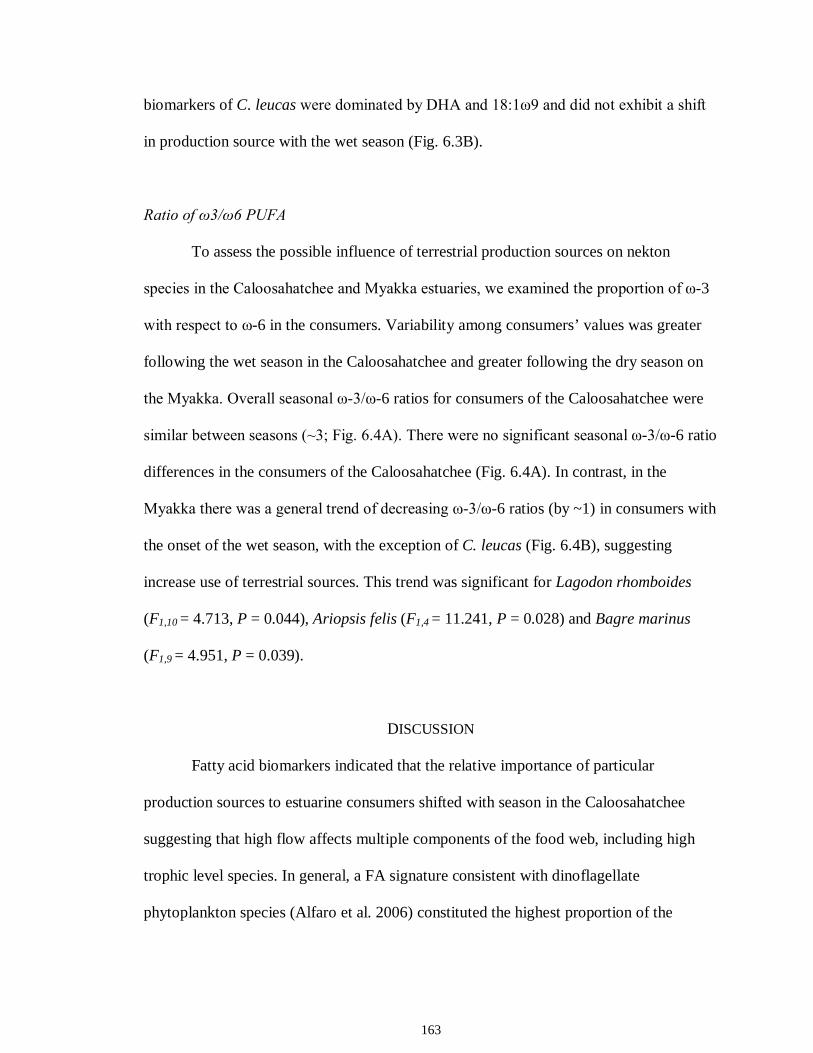
163

biomarkers of C. leucas were dominated by DHA and 18:1ω9 and did not exhibit a shift

in production source with the wet season (Fig. 6.3B).

Ratio of ω3/ω6 PUFA

To assess the possible influence of terrestrial production sources on nekton

species in the Caloosahatchee and Myakka estuaries, we examined the proportion of ω-3

with respect to ω-6 in the consumers. Variability among consumers’ values was greater

following the wet season in the Caloosahatchee and greater following the dry season on

the Myakka. Overall seasonal ω-3/ω-6 ratios for consumers of the Caloosahatchee were

similar between seasons (~3; Fig. 6.4A). There were no significant seasonal ω-3/ω-6 ratio

differences in the consumers of the Caloosahatchee (Fig. 6.4A). In contrast, in the

Myakka there was a general trend of decreasing ω-3/ω-6 ratios (by ~1) in consumers with

the onset of the wet season, with the exception of C. leucas (Fig. 6.4B), suggesting

increase use of terrestrial sources. This trend was significant for Lagodon rhomboides

(F1,10 = 4.713, P = 0.044), Ariopsis felis (F1,4 = 11.241, P = 0.028) and Bagre marinus

(F1,9 = 4.951, P = 0.039).

DISCUSSION

Fatty acid biomarkers indicated that the relative importance of particular

production sources to estuarine consumers shifted with season in the Caloosahatchee

suggesting that high flow affects multiple components of the food web, including high

trophic level species. In general, a FA signature consistent with dinoflagellate

phytoplankton species (Alfaro et al. 2006) constituted the highest proportion of the

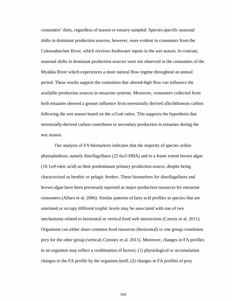
164

consumers’ diets, regardless of season or estuary sampled. Species-specific seasonal

shifts in dominant production sources, however, were evident in consumers from the

Caloosahatchee River, which receives freshwater inputs in the wet season. In contrast,

seasonal shifts in dominant production sources were not observed in the consumers of the

Myakka River which experiences a more natural flow regime throughout an annual

period. These results support the contention that altered-high flow can influence the

available production sources in estuarine systems. Moreover, consumers collected from

both estuaries showed a greater influence from terrestrially derived allochthonous carbon

following the wet season based on the ω3/ω6 ratios. This supports the hypothesis that

terrestrially-derived carbon contributes to secondary production in estuaries during the

wet season.

Our analysis of FA biomarkers indicates that the majority of species utilize

phytoplankton, namely dinoflagellates (22:6ω3-DHA) and to a lesser extent brown algae

(18:1ω9-oleic acid) as their predominant primary production source, despite being

characterized as benthic or pelagic feeders. These biomarkers for dinoflagellates and

brown algae have been previously reported as major production resources for estuarine

consumers (Alfaro et al. 2006). Similar patterns of fatty acid profiles in species that are

unrelated or occupy different trophic levels may be associated with one of two

mechanisms related to horizontal or vertical food web interactions (Czesny et al. 2011).

Organisms can either share common food resources (horizontal) or one group constitutes

prey for the other group (vertical; Czesney et al. 2011). Moreover, changes in FA profiles

in an organism may reflect a combination of factors; (1) physiological or accumulation

changes to the FA profile by the organism itself, (2) changes in FA profiles of prey

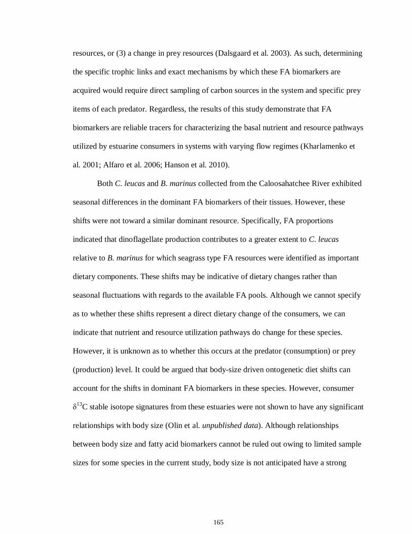
165

resources, or (3) a change in prey resources (Dalsgaard et al. 2003). As such, determining

the specific trophic links and exact mechanisms by which these FA biomarkers are

acquired would require direct sampling of carbon sources in the system and specific prey

items of each predator. Regardless, the results of this study demonstrate that FA

biomarkers are reliable tracers for characterizing the basal nutrient and resource pathways

utilized by estuarine consumers in systems with varying flow regimes (Kharlamenko et

al. 2001; Alfaro et al. 2006; Hanson et al. 2010).

Both C. leucas and B. marinus collected from the Caloosahatchee River exhibited

seasonal differences in the dominant FA biomarkers of their tissues. However, these

shifts were not toward a similar dominant resource. Specifically, FA proportions

indicated that dinoflagellate production contributes to a greater extent to C. leucas

relative to B. marinus for which seagrass type FA resources were identified as important

dietary components. These shifts may be indicative of dietary changes rather than

seasonal fluctuations with regards to the available FA pools. Although we cannot specify

as to whether these shifts represent a direct dietary change of the consumers, we can

indicate that nutrient and resource utilization pathways do change for these species.

However, it is unknown as to whether this occurs at the predator (consumption) or prey

(production) level. It could be argued that body-size driven ontogenetic diet shifts can

account for the shifts in dominant FA biomarkers in these species. However, consumer

δ13C stable isotope signatures from these estuaries were not shown to have any significant

relationships with body size (Olin et al. unpublished data). Although relationships

between body size and fatty acid biomarkers cannot be ruled out owing to limited sample

sizes for some species in the current study, body size is not anticipated have a strong

166

influence on the fatty acids biomarker profiles here. The lengths of individuals collected

for each species were not vastly different and larval and young juvenile individuals were

also not included in this study. Larval and young-of-year individuals commonly represent

life history stages when critical ontogenetic diets shifts and maternal/in-utero

mechanisms are known to influence biochemical tracer signatures (Czesney et al. 2011;

Olin et al. 2011).

Consumers sampled from the Myakka River showed a greater consumption of

allochthonous carbon following the wet season relative to conspecifics sampled following

the dry season based on ω3/ω6 ratios. This finding supports our hypothesis of increased

dependence on terrestrial subsidies by higher order consumers following the wet season.

It is well-established that estuaries are dependent on riverine inflows that provide

floodplain detritus and nutrients that facilitate high levels of primary and secondary

production (Chanton and Lewis 2002). That a similar shift toward allochthonous carbon

dependence does not exist in the Caloosahatchee is surprising. Previous studies have

demonstrated the increased dependence on terrestrially-derived sources following the wet

season in estuaries, particularly in studies tracking major storm events such as monsoons

(Wai et al. 2008; 2011; Abrantes and Sheaves 2010). The lack of significant decline in

the ω3/ω6 ratios in the Caloosahatchee could result from the magnitude of the flow being

so great that it provides large amounts of allochthonous materials that are used by

consumers throughout the year. Allochthonous fluxes of carbon to ecosystems are often

large (Pace et al. 2004) and therefore would be expected to be greater in the

Caloosahatchee as the drainage basin is nearly 2.5 times greater than that of the Myakka.

167

Mangrove contributions were identified as more important in the dry season

relative to the wet season in both estuaries, based on higher proportions of long-chain

saturated fatty acids (LCSFA) in the consumers’ tissues. These results support the

findings of Meziane and Tsuchiya (2000) whereby mangrove contributions to the diets of

estuarine consumer species are greater when flow regimes are low. Dependence on

mangroves declined in all consumers in both estuaries with the onset of the wet season,

with the exception of C. sapidus that showed an increased proportion of mangrove in

their tissues. Although mangrove forests are often considered to be highly productive, a

number of studies have challenged the paradigm that mangroves provide a major source

of nutrients to estuarine communities (Loneragan et al. 1997; Kieckbusch et al. 2004;

Heithaus et al. 2011). Based on stable isotopes, Heithaus et al. (2011) found that

mangroves did not contribute greatly to the carbon supply in a mangrove estuary in

Australia. Kieckbush et al. (2004) made a similar conclusion for a tropical lagoon in the

Bahamas. In contrast, Alfaro et al. (2006) demonstrated that mangrove detritus dominates

the suspended organic matter (SOM) fraction in estuarine waters and also concluded that

grazing and filter feeding species have high reliance on these materials based on their

LCSFA biomarker profiles. However, Heithaus et al. (2011) and Kieckbusch et al. (2004)

quantified carbon stable isotope signatures in leaves as opposed to SOM as the primary

mangrove component in consumers’ diets. Mangrove leaves are difficult to digest and are

generally broken down through bacterial action in the sediments which could alter the

stable isotope values (Hall et al. 2006). Therefore, the decrease in mangrove contribution

may be a result of the flushing of the SOM from estuaries with high flow or a shift in

bacterial composition and abundance. In any event, the greater proportions of LCSFA

168

observed in species sampled during the dry season suggest a greater availability of

mangrove derived resources in the system at this time.

Conclusions

Seasonal variation in nutrient and resource availability at the base of aquatic food

webs is tied to nutrient fluxes and physical conditions which in turn affect food resources

for primary, secondary and higher trophic level consumers. Consequently, quantifying

the temporal variability in such basal resources of an aquatic food web remains

challenging. Characterizing the seasonal presence and abundances of the various primary

production and organic matter sources in estuaries is critical to resolve the specific

trophic responses of consumers to extreme flow events. The application of FA

biomarkers provides a context to begin to understand seasonal resource and nutrient

dynamics with relatively minimal sampling effort. However, sampling production

sources is extremely important for comparing and resolving seasonal composition and

dynamics of FA biomarkers across season, conspecifics and estuaries. Such studies

provide valuable information for understanding shifts in carbon pathways and the

responses of estuarine nekton species to high freshwater flow events. While quantitative

estimates of diet using fatty acid profiles were not achieved here, our findings provide a

general baseline to assess food web relationships influenced by extreme flow events. The

results of the current study using FA biomarkers clearly distinguish seasonal dynamics in

high trophic level species, a result not attained using stable isotopes (Olin et al.

submitted). Under this consideration, FA profiles quantified in estuarine consumers may

169

provide greater resolution with respect toward characterizing the specific production

resources impacted by anthropogenically altered flow events.

REFERENCES

Abrantes K.G. & Sheaves M. 2010. Importance of freshwater flow in terrestrial-aquatic energetic connectivity in intermittently connected estuaries of tropical Australia. Marine Biology 157:2071–2086. Alfaro A.C., Thomas F., Sergent L. & Duxbury M. 2006. Identification of trophic interactions within an estuarine food web (northern New Zealand) using fatty acid biomarkers and stable isotopes. Estuarine, Coastal and Shelf Science 70:271–286. Arts M.T., Brett M.T. & Kainz M.J. 2009. Lipids in Aquatic Ecosystems. Springer Verlag, New York. Arts M.T. 1999. Lipids in freshwater zooplankton: selected ecological and physiological aspects. In: Lipids in Freshwater Ecosystems (M.T. Arts and B.C. Wainman, Eds.), Springer Verlag, New York. Barnes T. 2005. Caloosahatchee Estuary conceptual ecological model. Wetlands 25:884–897. Bligh E.G. & Dyer W.J. 1959. A rapid method of total lipid extraction and purification. Canadian Journal of Biochemistry and Physiology 37:911–917. Bradshaw C.J.A., Hindell N.J., Phillips K.L., Wilson G. & Nichols P.D. 2003. You are what you eat: describing the foraging ecology of southern elephant seals (Mirounga leonina) using blubber fatty acids. Proceedings of the Royal Society of London B 270:1283–1292. Budge S.M., Iverson S.J. & Koopman H.N. 2006. Studying trophic ecology in marine ecosystems using fatty acids: a primer on analysis and interpretation. Marine Mammal Science 22:759–801. Budge S.M. & Parrish C.C. 1998. Lipid biochemistry of plankton, settling matter and sediments in Trinity Bay, Newfoundland. II Fatty acids. Organic Geochemistry 29:1547–1559. Chanton J. & Lewis F.G. 2002. Examination of coupling between primary and secondary production in a river-dominated estuary: Apalachicola Bay, Florida, USA. Limnology and Oceanography 47:683–697.

170

Czesny J., Rinchard J., Hanson S.D., Dettmers J.M. & Dabrowski K. 2011. Fatty acid signatures of Lake Michigan prey fish and invertebrates: among-species differences and spatiotemporal variability. Canadian Journal of Fisheries and Aquatic Sciences 68:1211–1230. Dalsgaard J. & St. John M. 2004. Fatty acid biomarkers: validation of food web and trophic markers using 13C-labaled fatty acids in juvenile sandeel (Ammodytes tobianus). Canadian Journal of Fisheries and Aquatic Sciences 61:1671–1680. Dalsgaard J., John M., Katter G., Muller-Navarra D. & Hagen W. 2003. Fatty acid trophic markers in the pelagic marine environment. Advances in Marine Biology 46:225–340. Darnaude A.M. 2005. Fish ecology and terrestrial carbon use in coastal areas: implications for marine fish production. Journal of Animal Ecology 74:864–876. Doering P.H., Chamberlain R.H. & Haunert D.E. 2002. Using submerged aquatic vegetation to establish minimum and maximum freshwater inflows to the Caloosahatchee estuary, Florida. Estuaries 25:1343–1354. Doering P.H. & Chamberlain R.H. 1998. Water quality in the Caloosahatchee Estuary, San Carlos Bay and Pine Island Sound. In: Proceedings of the Charlotte Harbor Public Conference and Technical Symposium, Technical Report No. 98-02, Charlotte Harbor National Estuary Program, Punta Gorda, FL, pp. 229–240. Flaig E.G. & Capece J. 1998. Water use and runoff in the Caloosahatchee watershed. In: Proceedings of the Charlotte Harbor Public Conference and Technical Symposium, Technical Report No. 98-02, Charlotte Harbor National Estuary Program, Punta Gorda, FL, pp. 73–80. Hall D., Lee S.Y. & Meziane T. 2006. Fatty acids as trophic tracers in an experimental estuarine food chain: tracer transfer. Journal of Experimental Marine Biology and Ecology 336:42–53. Hanson C.E., Hyndes G.A. & Wang S.F. 2010. Differentiation of benthic marine primary producers using stable isotopes and fatty acids: implications to food web studies. Aquatic Botany 93:114–122. Hebert C.E., Weseloh D.V.C., Gauthier L.T., Arts M.T. & Letcher R.J. 2009. Biochemical tracers reveal intra-specific differences in the food webs utilized by individual seabirds. Oecologia 160:15–23. Hebert C.E., Arts M.T. & Weseloh D.V.C. 2006. Ecological tracers can quantify food web structure and change. Environmental Science and Technology 40:5618–5623.

171

Heithaus E.R., Heithaus P.A., Heithaus M.R., Burkholder D. & Layman C.A. 2011. Trophic dynamics in a relatively pristine subtropical fringing mangrove community. Marine Ecology Progress Series 428:49–61. Hobson K.A., Fisk A.T., Karnovsky N., Holst M., Gagnon J.M. & Fortier M. 2002. A stable isotope (δ13C, δ15N) model for the North Water food web: implications for evaluating trophodynamics and the flow of energy and contaminants Deep-Sea Research II 49:5131–5150. Johns R.B., Nichols P.D. & Perry G.J. 1979. Fatty acid composition of ten marine algae from Australia waters. Phytochemistry 18:799–802. Kang C.K., Kim J.B., Lee K.S., Lee P.Y. & Hong J.S. 2003. Trophic importance of benthic microalgae to macrozoobenthos in coastal bay systems in Korea: dual stable C and N isotope analyses. Marine Ecology Progress Series 259:79–92. Kharlamenko V.I., Kiyashko S.I., Imbs A.B. & Vyshkvartzev D.I. 2001. Identification of food sources of invertebrates from the seagrass Zostera marina community using carbon and sulfur stable isotope ratio and fatty acid analyses. Marine Ecology Progress Series 220:103–117. Kieckbusch D.K., Koch M.S., Serafy J.E. & Anderson W.T. 2004. Trophic linkages among primary producers and consumers in fringing mangroves of subtropical lagoons. Bulletin of Marine Science 74:271-285. Koussoroplis A.M., Bec A., Perga M.E., Koutrakis E., Bourdier G. & Desvilettes C. 2011. Fatty acid transfer in the food web of coastal Mediterranean lagoon: evidence for high arachidonic acid retention in fish. Estuarine, Coastal and Shelf Science 91:450–461. Koussoroplis A.M., Lemarchand C., Bec A., Desvilettes C., Amblard C., Fournier C., Berny P. & Bourdier G. 2008. From aquatic to terrestrial food webs: decrease of the docosahexaenoic acid/linoleic acid ratio. Lipids 43:461–466. Livingston R.J., Niu X., Lewis G. & Woodsum G.C. 1997. Freshwater input to a gulf estuary: long-term control of trophic organization. Ecological Applications 7:277–299. Loneragan N.R., Bunn S.E., & Kellaway D.M. 1997. Are mangroves and seagrass sources for penaeid prawns in a tropical Australian estuary? A multiple stable-isotope study. Marine Biology 130:289–300. McLeod R.J. & Wing S.R. 2009. Strong pathways for incorporation of terrestrially derived organic matter into benthic communities. Estuarine, Coastal and Shelf Science 82:645–653.

172

Meziane T. & Tsuchiya M. 2000. Fatty acids as tracers of organic matter in the sediment and food web of a mangrove/intertidal flat ecosystem, Okinawa, Japan. Marine Ecology Progress Series 200:49–57. Mfilinge P.L., Meziane T., Bachok Z. & Tsuchiya M. 2005. Litter dynamics and particulate organic matter outwelling from a subtropical mangrove in Okinawa Island, South Japan. Estuarine, Coastal and Shelf Science 63:301–313. Napolitano G.E., Pollero R.J., Gayoso A.M., Macdonald B.A. & Thompson R.J. 1997. Fatty acids as trophic markers of phytoplankton blooms in the Bahía Blanca Estuary (Buenos Aires, Argentina) and in Trinity Bay (Newfoundland, Canada). Biochemical Systematics and Ecology 25:739–755. Nordin L.J., Arts M.T., Johannsson O.E. & Taylor W.D. 2008. An evaluation of the diet of Mysis relicta using gut contents and fatty acid profiles in lakes with and without the invader Bythotrephes longimanus (Onychopoda, Ceropagidae). Aquatic Ecology 42:421–436. Oksanen J. 2011. Multivariate analysis of ecological communities in R: vegan tutorial. Olin J.A., Stevens P.W., Rush S.A., Hussey N.E. & Fisk A.T. Loss of seasonal variability in nekton community structure in a tidal river: evidence for homogenization in a flow-altered system. Ecological Applications in review: 17 October 2011.

Olin J.A., MacNeil M.A., Rush S.A. & Fisk A.T. 2011. Isotopic ratios reveal mixed seasonal variation among fishes from two subtropical estuarine systems. Estuaries and Coasts doi: 10.1007/s12237-011-9467-6

Olin J.A., Hussey N.E., Fritts M., Heupel M.R., Simpfendorfer C.A., Poulakis G.R. & Fisk A.T. 2011. Maternal meddling in neonatal sharks: implication for interpreting stable isotopes in young animals. Rapid Communications in Mass Spectrometry 25:1008–1016. Olsen, Y. 1999. Lipids and essential fatty acids in aquatic food webs: What can freshwater ecologists learn from mariculture? In: Lipids in Freshwater Ecosystems (M.T. Arts and B.C. Wainman, Eds.), pp. 161–202. Springer Verlag, New York. Pace M.L., Cole J.J., Carpenter S.R., Kitchell J.F., Hodgson J.R., Van de Bogert M.C., Bade D.L., Kritzberg E.S. & Bastviken D. 2004. Whole-lake carbon-13 additions reveal terrestrial support of aquatic food webs. Nature 427:240–243. Parrish C.C., Abrajano T.A., Budge S.M., Helleur R.J., Hudson E.D., Pulchan K. & Ramos, C. 2000. Lipid and phenolic biomarkers in marine ecosystems: analysis and applications. In: The Handbook of Environmental Chemistry, vol. 5 Part D. Marine Chemistry (P. Wangersky, Ed.), Springer-Verlag, Berlin.

173

R Development Core Team. 2011. R: A language and environment for statistical computing. R Foundation for Statistical Computing, Vienna, Austria. Richoux N.B. & Froneman P.W. 2008. Trophic ecology of dominant zooplankton and macrofauna in a temperate, oligotrophic South African estuary: a fatty acid approach. Marine Ecology Progress Series 357:121–137. Sigurgisladottir S., Lall S.P., Parrish C.C. & Ackman R.G. 1992. Cholestane as a digestibility marker in the absorption of polyunsaturated fatty acid ethyl esters in the Atlantic salmon. Lipids 27:418–424. Smith R.J., Hobson K.A., Koopman H.N. & Lavigne D.M. 2005. Distinguishing between populations of fresh- and salt-water harbor seals (Phoca vitulina) using stable-isotope ratios and fatty acid profiles. Canadian Journal of Fisheries and Aquatic Sciences 53: 272–279. South Florida Water Management District. 2008. Caloosahatchee Water Management Plan. South Florida Water Management District, West Palm Beach, FL. Turner J.P. & Rooker J.R. 2006. Fatty acid composition of flora and fauna associated with Sargassum mats in the Gulf of Mexico. Marine Biology 149:1025–1036. Volkman J.K., Johns R.B., Gillian F.T. & Perry G.I. 1980. Microbial lipids of an intertidal sediment. I. Fatty acids and hydrocarbons. Geochimica et Cosmochimica Acta 44:1133–1143. Wai T.K., Leung K.M.Y., Sin S.Y.T, Cornish A., Dudgeon D. & Williams G.A. 2011. Spatial, seasonal, and ontogenetic variations in the significance of detrital pathways and terrestrial carbon for a benthic shark. Chiloscyllium plagiosum (Hemiscylliidae), in a tropical estuary. Limnology and Oceanography 56:1035–1053. Wai T.K., Ng J.S.S. & Leung K.M.Y. 2008. The source and fate of organic matter and the significance of detrital pathways in a tropical coastal ecosystem. Limnology and Oceanography 53:1479–1492. Wannigama G.P., Volkman J.K., Gillan F.T., Nichols P.D. & Johns R.B. 1981: a comparison of lipid components of the fresh and dead leaves and pneumatophores of the mangrove Avicennia marina. Phytochemistry 20:659–666.

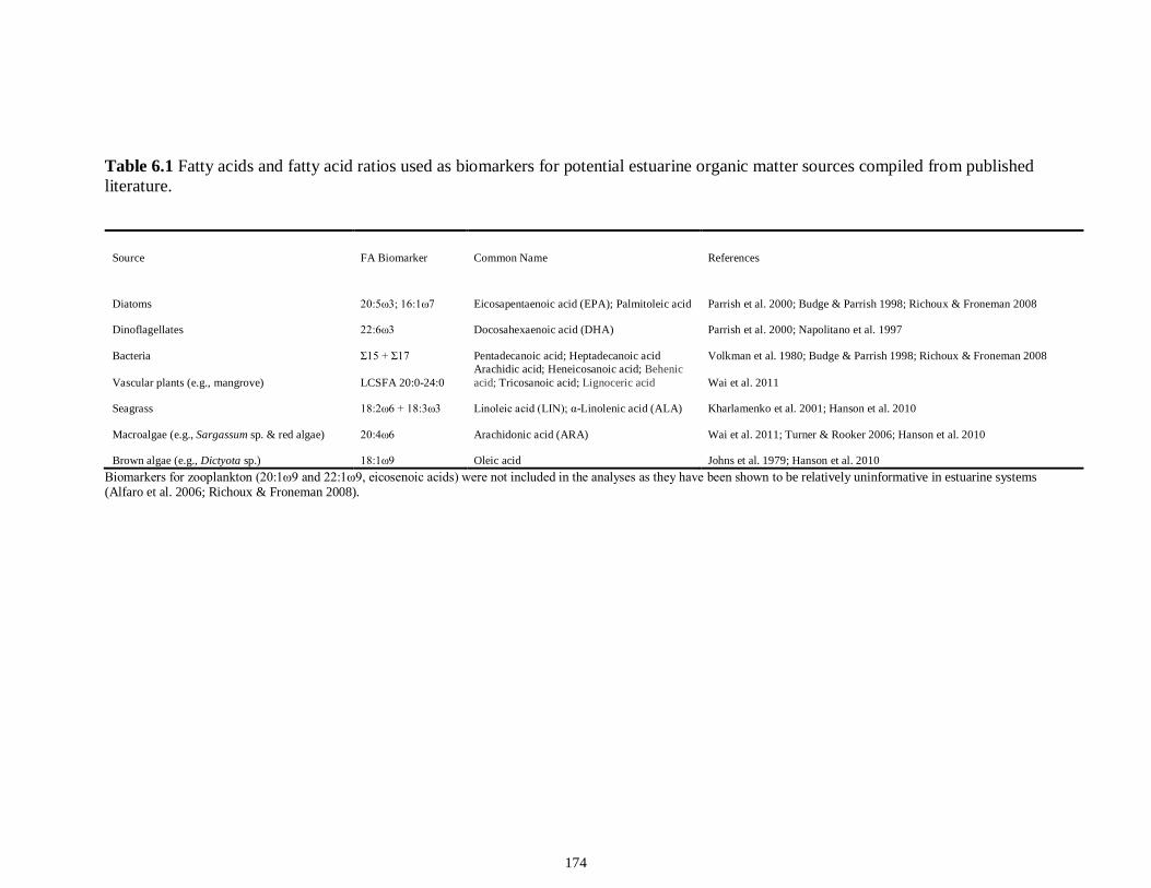
174

Table 6.1 Fatty acids and fatty acid ratios used as biomarkers for potential estuarine organic matter sources compiled from published literature.

Source FA Biomarker Common Name References

Diatoms 20:5ω3; 16:1ω7 Eicosapentaenoic acid (EPA); Palmitoleic acid Parrish et al. 2000; Budge & Parrish 1998; Richoux & Froneman 2008

Dinoflagellates 22:6ω3 Docosahexaenoic acid (DHA) Parrish et al. 2000; Napolitano et al. 1997

Bacteria Σ15 + Σ17 Pentadecanoic acid; Heptadecanoic acid Volkman et al. 1980; Budge & Parrish 1998; Richoux & Froneman 2008

Vascular plants (e.g., mangrove) LCSFA 20:0-24:0 Arachidic acid; Heneicosanoic acid; Behenic acid; Tricosanoic acid; Lignoceric acid Wai et al. 2011

Seagrass 18:2ω6 + 18:3ω3 Linoleic acid (LIN); α-Linolenic acid (ALA) Kharlamenko et al. 2001; Hanson et al. 2010

Macroalgae (e.g., Sargassum sp. & red algae) 20:4ω6 Arachidonic acid (ARA) Wai et al. 2011; Turner & Rooker 2006; Hanson et al. 2010

Brown algae (e.g., Dictyota sp.) 18:1ω9 Oleic acid Johns et al. 1979; Hanson et al. 2010 Biomarkers for zooplankton (20:1ω9 and 22:1ω9, eicosenoic acids) were not included in the analyses as they have been shown to be relatively uninformative in estuarine systems (Alfaro et al. 2006; Richoux & Froneman 2008).

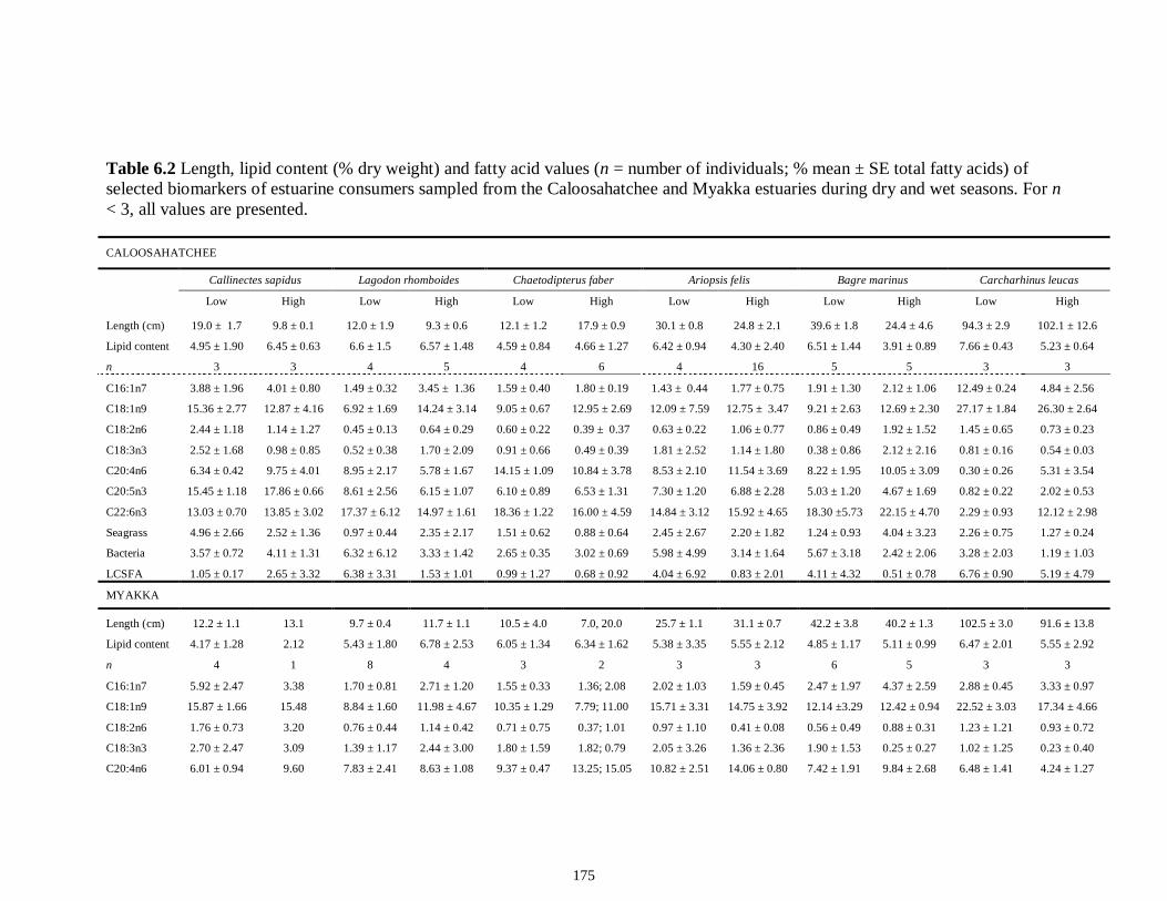
175

Table 6.2 Length, lipid content (% dry weight) and fatty acid values (n = number of individuals; % mean ± SE total fatty acids) of selected biomarkers of estuarine consumers sampled from the Caloosahatchee and Myakka estuaries during dry and wet seasons. For n < 3, all values are presented.

CALOOSAHATCHEE

Callinectes sapidus Lagodon rhomboides Chaetodipterus faber Ariopsis felis Bagre marinus Carcharhinus leucas

Low High Low High Low High Low High Low High Low High

Length (cm) 19.0 ± 1.7 9.8 ± 0.1 12.0 ± 1.9 9.3 ± 0.6 12.1 ± 1.2 17.9 ± 0.9 30.1 ± 0.8 24.8 ± 2.1 39.6 ± 1.8 24.4 ± 4.6 94.3 ± 2.9 102.1 ± 12.6

Lipid content 4.95 ± 1.90 6.45 ± 0.63 6.6 ± 1.5 6.57 ± 1.48 4.59 ± 0.84 4.66 ± 1.27 6.42 ± 0.94 4.30 ± 2.40 6.51 ± 1.44 3.91 ± 0.89 7.66 ± 0.43 5.23 ± 0.64

n 3 3 4 5 4 6 4 16 5 5 3 3

C16:1n7 3.88 ± 1.96 4.01 ± 0.80 1.49 ± 0.32 3.45 ± 1.36 1.59 ± 0.40 1.80 ± 0.19 1.43 ± 0.44 1.77 ± 0.75 1.91 ± 1.30 2.12 ± 1.06 12.49 ± 0.24 4.84 ± 2.56

C18:1n9 15.36 ± 2.77 12.87 ± 4.16 6.92 ± 1.69 14.24 ± 3.14 9.05 ± 0.67 12.95 ± 2.69 12.09 ± 7.59 12.75 ± 3.47 9.21 ± 2.63 12.69 ± 2.30 27.17 ± 1.84 26.30 ± 2.64

C18:2n6 2.44 ± 1.18 1.14 ± 1.27 0.45 ± 0.13 0.64 ± 0.29 0.60 ± 0.22 0.39 ± 0.37 0.63 ± 0.22 1.06 ± 0.77 0.86 ± 0.49 1.92 ± 1.52 1.45 ± 0.65 0.73 ± 0.23

C18:3n3 2.52 ± 1.68 0.98 ± 0.85 0.52 ± 0.38 1.70 ± 2.09 0.91 ± 0.66 0.49 ± 0.39 1.81 ± 2.52 1.14 ± 1.80 0.38 ± 0.86 2.12 ± 2.16 0.81 ± 0.16 0.54 ± 0.03

C20:4n6 6.34 ± 0.42 9.75 ± 4.01 8.95 ± 2.17 5.78 ± 1.67 14.15 ± 1.09 10.84 ± 3.78 8.53 ± 2.10 11.54 ± 3.69 8.22 ± 1.95 10.05 ± 3.09 0.30 ± 0.26 5.31 ± 3.54

C20:5n3 15.45 ± 1.18 17.86 ± 0.66 8.61 ± 2.56 6.15 ± 1.07 6.10 ± 0.89 6.53 ± 1.31 7.30 ± 1.20 6.88 ± 2.28 5.03 ± 1.20 4.67 ± 1.69 0.82 ± 0.22 2.02 ± 0.53

C22:6n3 13.03 ± 0.70 13.85 ± 3.02 17.37 ± 6.12 14.97 ± 1.61 18.36 ± 1.22 16.00 ± 4.59 14.84 ± 3.12 15.92 ± 4.65 18.30 ±5.73 22.15 ± 4.70 2.29 ± 0.93 12.12 ± 2.98

Seagrass 4.96 ± 2.66 2.52 ± 1.36 0.97 ± 0.44 2.35 ± 2.17 1.51 ± 0.62 0.88 ± 0.64 2.45 ± 2.67 2.20 ± 1.82 1.24 ± 0.93 4.04 ± 3.23 2.26 ± 0.75 1.27 ± 0.24

Bacteria 3.57 ± 0.72 4.11 ± 1.31 6.32 ± 6.12 3.33 ± 1.42 2.65 ± 0.35 3.02 ± 0.69 5.98 ± 4.99 3.14 ± 1.64 5.67 ± 3.18 2.42 ± 2.06 3.28 ± 2.03 1.19 ± 1.03

LCSFA 1.05 ± 0.17 2.65 ± 3.32 6.38 ± 3.31 1.53 ± 1.01 0.99 ± 1.27 0.68 ± 0.92 4.04 ± 6.92 0.83 ± 2.01 4.11 ± 4.32 0.51 ± 0.78 6.76 ± 0.90 5.19 ± 4.79

MYAKKA

Length (cm) 12.2 ± 1.1 13.1 9.7 ± 0.4 11.7 ± 1.1 10.5 ± 4.0 7.0, 20.0 25.7 ± 1.1 31.1 ± 0.7 42.2 ± 3.8 40.2 ± 1.3 102.5 ± 3.0 91.6 ± 13.8

Lipid content 4.17 ± 1.28 2.12 5.43 ± 1.80 6.78 ± 2.53 6.05 ± 1.34 6.34 ± 1.62 5.38 ± 3.35 5.55 ± 2.12 4.85 ± 1.17 5.11 ± 0.99 6.47 ± 2.01 5.55 ± 2.92

n 4 1 8 4 3 2 3 3 6 5 3 3

C16:1n7 5.92 ± 2.47 3.38 1.70 ± 0.81 2.71 ± 1.20 1.55 ± 0.33 1.36; 2.08 2.02 ± 1.03 1.59 ± 0.45 2.47 ± 1.97 4.37 ± 2.59 2.88 ± 0.45 3.33 ± 0.97

C18:1n9 15.87 ± 1.66 15.48 8.84 ± 1.60 11.98 ± 4.67 10.35 ± 1.29 7.79; 11.00 15.71 ± 3.31 14.75 ± 3.92 12.14 ±3.29 12.42 ± 0.94 22.52 ± 3.03 17.34 ± 4.66

C18:2n6 1.76 ± 0.73 3.20 0.76 ± 0.44 1.14 ± 0.42 0.71 ± 0.75 0.37; 1.01 0.97 ± 1.10 0.41 ± 0.08 0.56 ± 0.49 0.88 ± 0.31 1.23 ± 1.21 0.93 ± 0.72

C18:3n3 2.70 ± 2.47 3.09 1.39 ± 1.17 2.44 ± 3.00 1.80 ± 1.59 1.82; 0.79 2.05 ± 3.26 1.36 ± 2.36 1.90 ± 1.53 0.25 ± 0.27 1.02 ± 1.25 0.23 ± 0.40

C20:4n6 6.01 ± 0.94 9.60 7.83 ± 2.41 8.63 ± 1.08 9.37 ± 0.47 13.25; 15.05 10.82 ± 2.51 14.06 ± 0.80 7.42 ± 1.91 9.84 ± 2.68 6.48 ± 1.41 4.24 ± 1.27

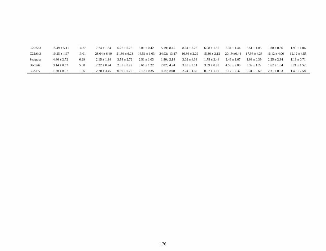
176

C20:5n3 15.49 ± 5.11 14.27 7.74 ± 1.34 6.27 ± 0.76 6.01 ± 0.42 5.19; 8.45 8.04 ± 2.28 6.98 ± 1.56 6.34 ± 1.44 5.51 ± 1.05 1.80 ± 0.36 1.99 ± 1.06

C22:6n3 10.25 ± 1.97 13.01 28.04 ± 6.49 21.30 ± 6.23 16.51 ± 1.03 24.93; 13.17 16.36 ± 2.29 15.30 ± 2.12 20.19 ±6.44 17.96 ± 4.23 16.12 ± 4.00 12.12 ± 4.55

Seagrass 4.46 ± 2.72 6.29 2.15 ± 1.34 3.58 ± 2.72 2.51 ± 1.03 1.80; 2.18 3.02 ± 4.38 1.78 ± 2.44 2.46 ± 1.67 1.08 ± 0.39 2.25 ± 2.34 1.16 ± 0.71

Bacteria 3.14 ± 0.57 5.68 2.22 ± 0.24 2.35 ± 0.22 3.61 ± 1.22 2.82; 4.24 3.85 ± 3.11 3.69 ± 0.98 4.53 ± 2.88 3.32 ± 1.22 1.62 ± 1.84 3.21 ± 1.52

LCSFA 1.30 ± 0.57 1.86 2.70 ± 3.45 0.90 ± 0.70 2.10 ± 0.35 0.00; 0.00 2.24 ± 1.52 0.57 ± 1.00 2.17 ± 2.32 0.31 ± 0.69 2.31 ± 0.63 1.49 ± 2.58

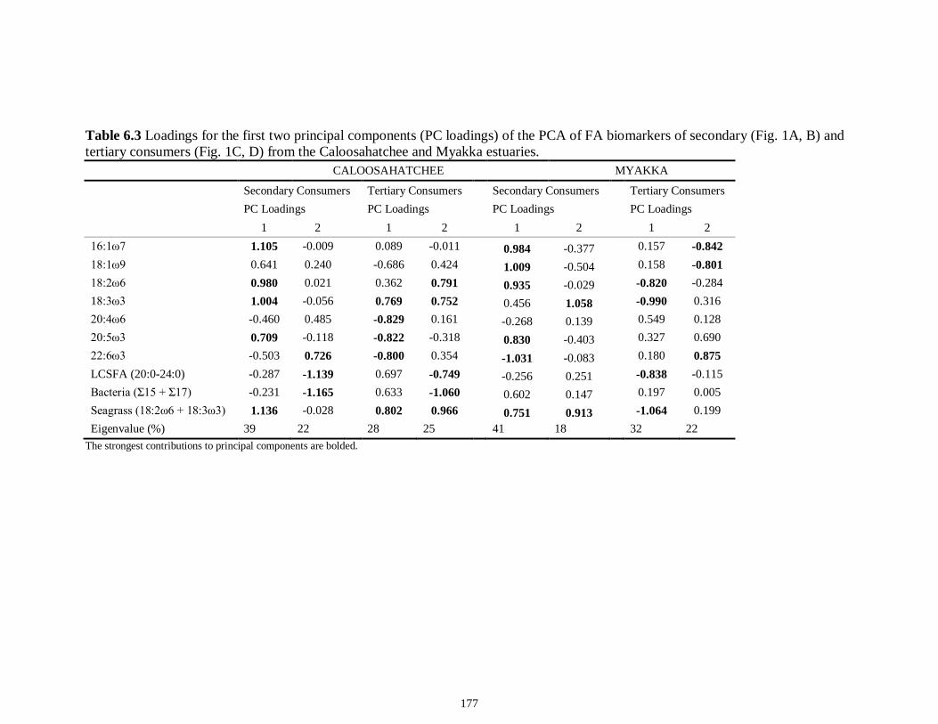
177

Table 6.3 Loadings for the first two principal components (PC loadings) of the PCA of FA biomarkers of secondary (Fig. 1A, B) and tertiary consumers (Fig. 1C, D) from the Caloosahatchee and Myakka estuaries.

CALOOSAHATCHEE MYAKKA

Secondary Consumers Tertiary Consumers Secondary Consumers Tertiary Consumers PC Loadings PC Loadings PC Loadings PC Loadings 1 2 1 2 1 2 1 2 16:1ω7 1.105 -0.009 0.089 -0.011 0.984 -0.377 0.157 -0.842 18:1ω9 0.641 0.240 -0.686 0.424 1.009 -0.504 0.158 -0.801 18:2ω6 0.980 0.021 0.362 0.791 0.935 -0.029 -0.820 -0.284 18:3ω3 1.004 -0.056 0.769 0.752 0.456 1.058 -0.990 0.316 20:4ω6 -0.460 0.485 -0.829 0.161 -0.268 0.139 0.549 0.128 20:5ω3 0.709 -0.118 -0.822 -0.318 0.830 -0.403 0.327 0.690 22:6ω3 -0.503 0.726 -0.800 0.354 -1.031 -0.083 0.180 0.875 LCSFA (20:0-24:0) -0.287 -1.139 0.697 -0.749 -0.256 0.251 -0.838 -0.115 Bacteria (Σ15 + Σ17) -0.231 -1.165 0.633 -1.060 0.602 0.147 0.197 0.005 Seagrass (18:2ω6 + 18:3ω3) 1.136 -0.028 0.802 0.966 0.751 0.913 -1.064 0.199 Eigenvalue (%) 39 22 28 25 41 18 32 22

The strongest contributions to principal components are bolded.

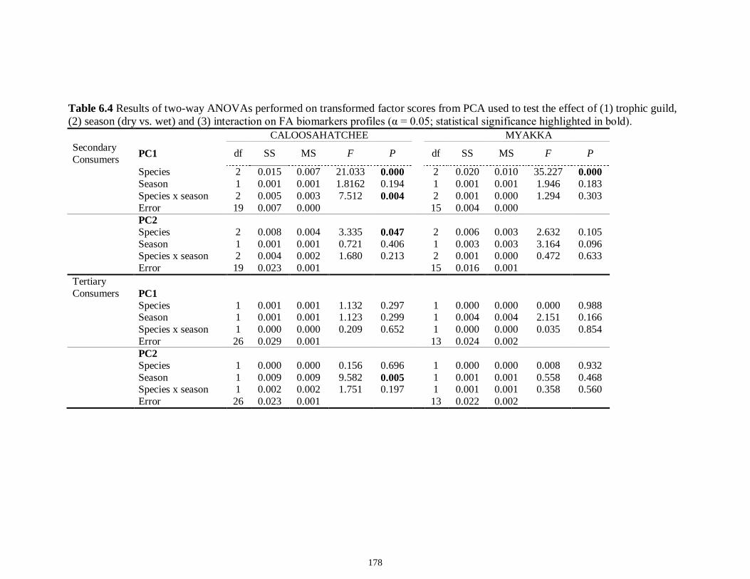
178

Table 6.4 Results of two-way ANOVAs performed on transformed factor scores from PCA used to test the effect of (1) trophic guild, (2) season (dry vs. wet) and (3) interaction on FA biomarkers profiles (α = 0.05; statistical significance highlighted in bold).

CALOOSAHATCHEE MYAKKA Secondary Consumers PC1 df SS MS F P df SS MS F P

Species 2 0.015 0.007 21.033 0.000 2 0.020 0.010 35.227 0.000 Season 1 0.001 0.001 1.8162 0.194 1 0.001 0.001 1.946 0.183 Species x season 2 0.005 0.003 7.512 0.004 2 0.001 0.000 1.294 0.303 Error 19 0.007 0.000 15 0.004 0.000 PC2 Species 2 0.008 0.004 3.335 0.047 2 0.006 0.003 2.632 0.105 Season 1 0.001 0.001 0.721 0.406 1 0.003 0.003 3.164 0.096 Species x season 2 0.004 0.002 1.680 0.213 2 0.001 0.000 0.472 0.633 Error 19 0.023 0.001 15 0.016 0.001 Tertiary Consumers PC1 Species 1 0.001 0.001 1.132 0.297 1 0.000 0.000 0.000 0.988 Season 1 0.001 0.001 1.123 0.299 1 0.004 0.004 2.151 0.166 Species x season 1 0.000 0.000 0.209 0.652 1 0.000 0.000 0.035 0.854 Error 26 0.029 0.001 13 0.024 0.002 PC2 Species 1 0.000 0.000 0.156 0.696 1 0.000 0.000 0.008 0.932 Season 1 0.009 0.009 9.582 0.005 1 0.001 0.001 0.558 0.468 Species x season 1 0.002 0.002 1.751 0.197 1 0.001 0.001 0.358 0.560 Error 26 0.023 0.001 13 0.022 0.002

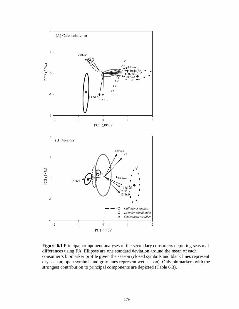
179

Figure 6.1 Principal component analyses of the secondary consumers depicting seasonal differences using FA. Ellipses are one standard deviation around the mean of each consumer’s biomarker profile given the season (closed symbols and black lines represent dry season; open symbols and gray lines represent wet season). Only biomarkers with the strongest contribution to principal components are depicted (Table 6.3).

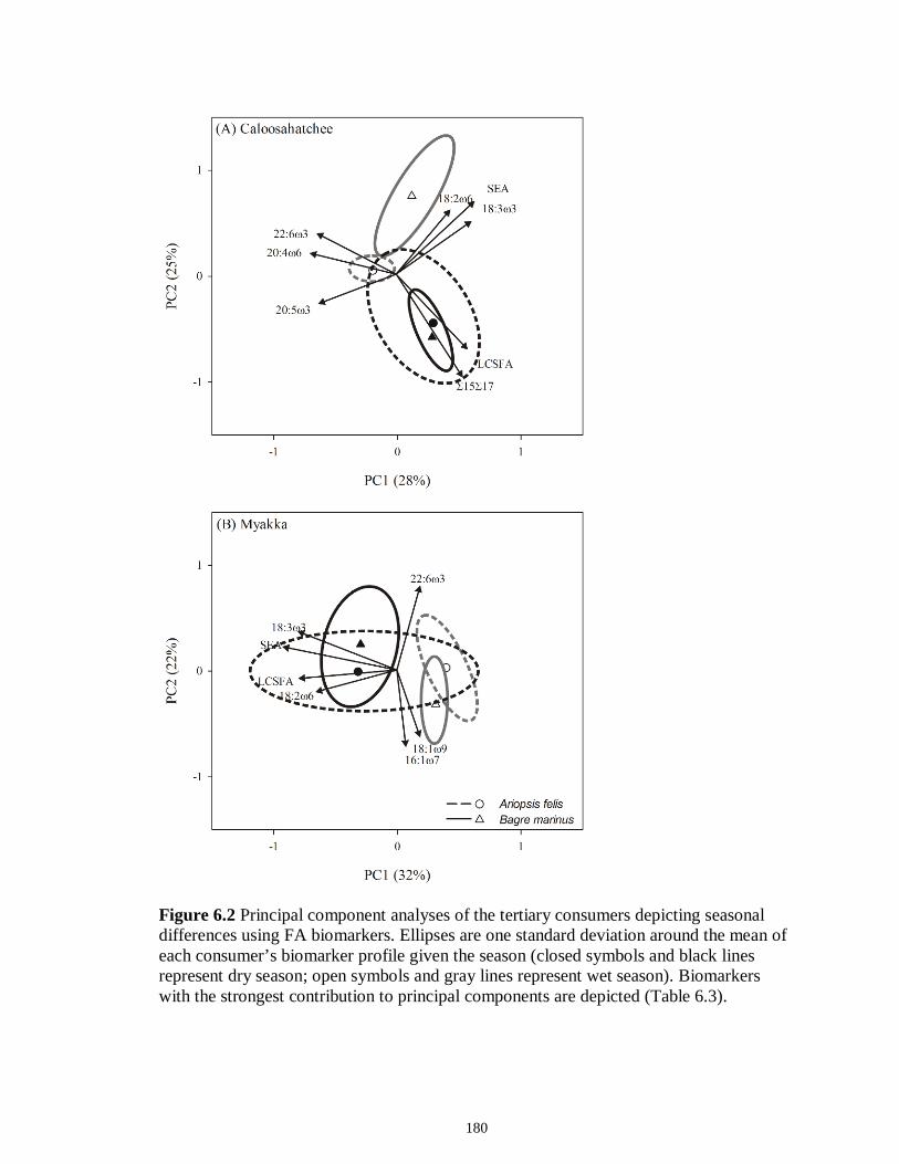
180

Figure 6.2 Principal component analyses of the tertiary consumers depicting seasonal differences using FA biomarkers. Ellipses are one standard deviation around the mean of each consumer’s biomarker profile given the season (closed symbols and black lines represent dry season; open symbols and gray lines represent wet season). Biomarkers with the strongest contribution to principal components are depicted (Table 6.3).

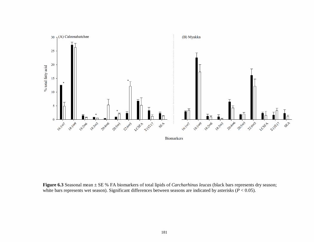
181

Figure 6.3 Seasonal mean ± SE % FA biomarkers of total lipids of Carcharhinus leucas (black bars represents dry season; white bars represents wet season). Significant differences between seasons are indicated by asterisks (P < 0.05).

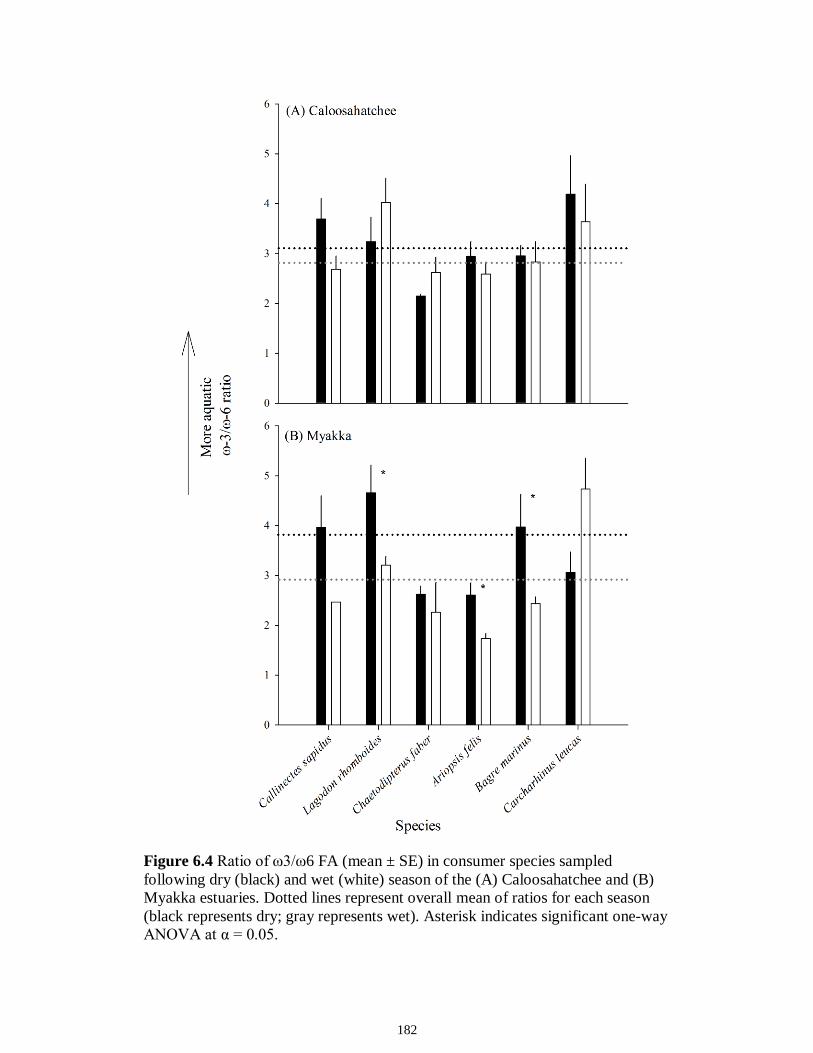
182

Figure 6.4 Ratio of ω3/ω6 FA (mean ± SE) in consumer species sampled following dry (black) and wet (white) season of the (A) Caloosahatchee and (B) Myakka estuaries. Dotted lines represent overall mean of ratios for each season (black represents dry; gray represents wet). Asterisk indicates significant one-way ANOVA at α = 0.05.

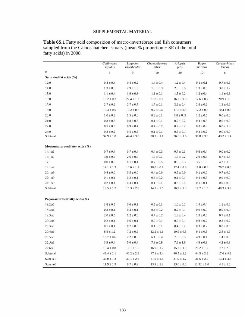
183

SUPPLEMENTAL MATERIAL

Table 6S.1 Fatty acid composition of macro-invertebrate and fish consumers sampled from the Caloosahatchee estuary (mean % proportion ± SE of the total fatty acids) in 2008.

Callinectes sapidus

Lagodon rhomboides

Chaetodipterus faber

Ariopsis felis

Bagre marinus

Carcharhinus leucas

n 6 9 10 20 10 6 Saturated fat acids (%)

12:0 0.4 ± 0.4 0.4 ± 0.2 1.4 ± 0.4 1.2 ± 0.4 0.1 ± 0.1 0.7 ± 0.6

14:0 1.3 ± 0.6 2.9 ± 1.0 1.6 ± 0.3 2.0 ± 0.5 1.3 ± 0.5 3.0 ± 1.2

15:0 1.1 ± 0.4 1.9 ± 0.3 1.1 ± 0.1 1.5 ± 0.2 1.2 ± 0.4 1.1 ± 0.6

16:0 15.2 ± 0.7 22.4 ± 1.7 21.8 ± 0.8 16.7 ± 0.8 17.6 ± 0.7 20.9 ± 1.5

17:0 2.7 ± 0.6 2.7 ± 0.7 1.7 ± 0.1 2.2 ± 0.4 2.8 ± 0.6 1.2 ± 0.3

18:0 10.3 ± 0.5 10.2 ± 0.7 9.7 ± 0.4 11.5 ± 0.5 12.2 ± 0.6 10.4 ± 0.5

20:0 1.0 ± 0.3 1.5 ± 0.6 0.3 ± 0.1 0.8 ± 0. 5 1.2 ± 0.5 0.0 ± 0.0

21:0 0.3 ± 0.3 0.8 ± 0.5 0.1 ± 0.1 0.2 ± 0.2 0.4 ± 0.3 0.0 ± 0.0

22:0 0.5 ± 0.3 0.9 ± 0.4 0.4 ± 0.2 0.2 ± 0.2 0.3 ± 0.3 6.0 ± 1.3

24:0 0.2 ± 0.2 0.5 ± 0.3 0.1 ± 0.1 0.3 ± 0.1 0.3 ± 0.2 0.0 ± 0.0 Subtotal 32.9 ± 1.8 44.4 ± 3.0 38.2 ± 1.1 36.6 ± 1.5 37.8 ± 3.0 43.2 ± 1.4

Monounsaturated fatty acids (%)

14:1ω5 0.7 ± 0.4 0.7 ± 0.4 0.4 ± 0.3 0.7 ± 0.3 0.6 ± 0.4 0.0 ± 0.0 16:1ω7 3.9 ± 0.6 2.6 ± 0.5 1.7 ± 0.1 1.7 ± 0.2 2.0 ± 0.4 8.7 ± 1.8

17:1 0.0 ± 0.0 0.1 ± 0.1 0.7 ± 0.5 0.9 ± 0.3 3.5 ± 1.5 4.2 ± 1.9 18:1ω9 14.1 ± 1.3 10.6 ± 1.7 10.8 ± 0.7 12.4 ± 0.9 11.0 ± 0.8 26.7 ± 0.8

20:1ω9 0.4 ± 0.0 0.5 ± 0.0 0.4 ± 0.0 0.5 ± 0.0 0.1 ± 0.0 0.7 ± 0.0 22:1ω9 0.1 ± 0.1 0.2 ± 0.1 0.3 ± 0.2 0.1 ± 0.1 0.4 ± 0.3 0.0 ± 0.0 24:1ω9 0.2 ± 0.1 0.3 ± 0.1 0.1 ± 0.1 0.3 ± 0.1 0.1 ± 0.1 0.0 ± 0.0

Subtotal 19.5 ± 1.7 15.3 ± 2.0 14.7 ± 1.5 16.9 ± 1.0 17.7 ± 1.5 40.3 ± 3.9

Polyunsaturated fatty acids (%)

18:2ω6 1.8 ± 0.5 0.6 ± 0.1 0.5 ± 0.1 1.0 ± 0.2 1.4 ± 0.4 1.1 ± 0.2

18:3ω6 0.3 ± 0.1 0.3 ± 0.1 0.4 ± 0.2 0.2 ± 0.1 0.0 ± 0.0 0.0 ± 0.0

18:3ω3 2.0 ± 0.5 1.2 ± 0.6 0.7 ± 0.2 1.3 ± 0.4 1.3 ± 0.6 0.7 ± 0.1

20:3ω6 0.2 ± 0.1 0.6 ± 0.1 0.9 ± 0.1 0.9 ± 0.1 0.8 ± 0.2 0.2 ± 0.2

20:3ω3 0.1 ± 0.1 0.7 ± 0.3 0.1 ± 0.1 0.4 ± 0.2 0.3 ± 0.2 0.0 ± 0.0

20:4ω6 8.8 ± 1.2 7.2 ± 0.9 12.2 ± 1.1 10.9 ± 0.8 9.1 ± 0.8 2.8 ± 1.5

20:5ω3 16.7 ± 0.6 7.2 ± 0.8 6.4 ± 0.4 7.0 ± 0.5 4.9 ± 0.4 1.4 ± 0.3

22:5ω3 3.9 ± 0.4 5.0 ± 0.4 7.8 ± 0.9 7.6 ± 1.6 4.9 ± 0.3 4.2 ± 0.8

22:6ω3 13.4 ± 0.8 16.1 ± 1.5 16.9 ± 1.2 15.7 ± 1.0 20.2 ± 1.7 7.2 ± 2.3

Subtotal 49.4 ± 2.1 40.2 ± 2.9 47.1 ± 2.4 46.5 ± 1.3 44.5 ± 2.8 17.6 ± 4.8

Sum ω-3 36.0 ± 1.2 30.1 ± 2.3 31.9 ± 1.4 31.9 ± 1.2 31.6 ± 2.0 13.4 ± 3.3

Sum ω-6 11.9 ± 1.3 8.7 ± 0.9 13.9 ± 1.2 13.0 ± 0.8 11.32 ± 1.0 4.1 ± 1.5

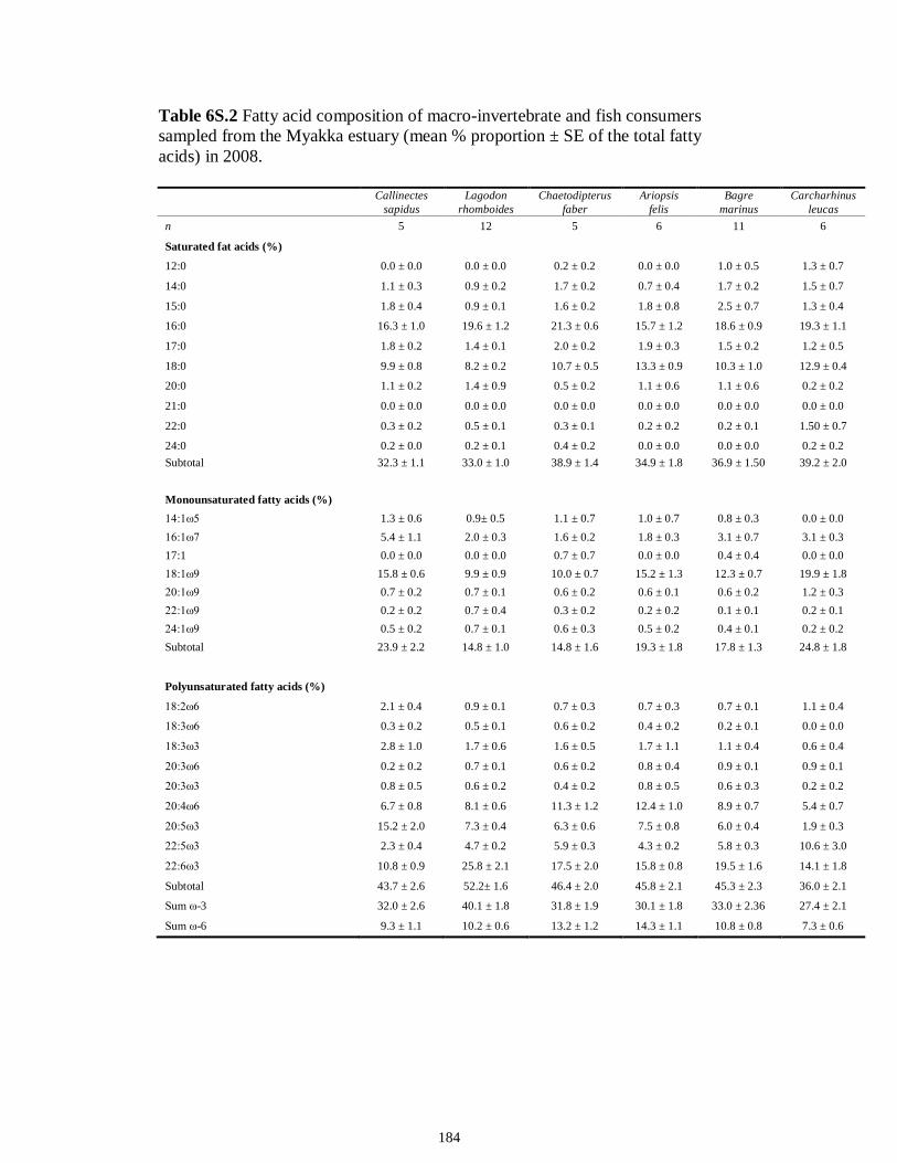
184

Table 6S.2 Fatty acid composition of macro-invertebrate and fish consumers sampled from the Myakka estuary (mean % proportion ± SE of the total fatty acids) in 2008.

Callinectes sapidus

Lagodon rhomboides

Chaetodipterus faber

Ariopsis felis

Bagre marinus

Carcharhinus leucas

n 5 12 5 6 11 6

Saturated fat acids (%)

12:0 0.0 ± 0.0 0.0 ± 0.0 0.2 ± 0.2 0.0 ± 0.0 1.0 ± 0.5 1.3 ± 0.7

14:0 1.1 ± 0.3 0.9 ± 0.2 1.7 ± 0.2 0.7 ± 0.4 1.7 ± 0.2 1.5 ± 0.7

15:0 1.8 ± 0.4 0.9 ± 0.1 1.6 ± 0.2 1.8 ± 0.8 2.5 ± 0.7 1.3 ± 0.4

16:0 16.3 ± 1.0 19.6 ± 1.2 21.3 ± 0.6 15.7 ± 1.2 18.6 ± 0.9 19.3 ± 1.1

17:0 1.8 ± 0.2 1.4 ± 0.1 2.0 ± 0.2 1.9 ± 0.3 1.5 ± 0.2 1.2 ± 0.5

18:0 9.9 ± 0.8 8.2 ± 0.2 10.7 ± 0.5 13.3 ± 0.9 10.3 ± 1.0 12.9 ± 0.4

20:0 1.1 ± 0.2 1.4 ± 0.9 0.5 ± 0.2 1.1 ± 0.6 1.1 ± 0.6 0.2 ± 0.2

21:0 0.0 ± 0.0 0.0 ± 0.0 0.0 ± 0.0 0.0 ± 0.0 0.0 ± 0.0 0.0 ± 0.0

22:0 0.3 ± 0.2 0.5 ± 0.1 0.3 ± 0.1 0.2 ± 0.2 0.2 ± 0.1 1.50 ± 0.7

24:0 0.2 ± 0.0 0.2 ± 0.1 0.4 ± 0.2 0.0 ± 0.0 0.0 ± 0.0 0.2 ± 0.2 Subtotal 32.3 ± 1.1 33.0 ± 1.0 38.9 ± 1.4 34.9 ± 1.8 36.9 ± 1.50 39.2 ± 2.0

Monounsaturated fatty acids (%) 14:1ω5 1.3 ± 0.6 0.9± 0.5 1.1 ± 0.7 1.0 ± 0.7 0.8 ± 0.3 0.0 ± 0.0 16:1ω7 5.4 ± 1.1 2.0 ± 0.3 1.6 ± 0.2 1.8 ± 0.3 3.1 ± 0.7 3.1 ± 0.3 17:1 0.0 ± 0.0 0.0 ± 0.0 0.7 ± 0.7 0.0 ± 0.0 0.4 ± 0.4 0.0 ± 0.0 18:1ω9 15.8 ± 0.6 9.9 ± 0.9 10.0 ± 0.7 15.2 ± 1.3 12.3 ± 0.7 19.9 ± 1.8 20:1ω9 0.7 ± 0.2 0.7 ± 0.1 0.6 ± 0.2 0.6 ± 0.1 0.6 ± 0.2 1.2 ± 0.3 22:1ω9 0.2 ± 0.2 0.7 ± 0.4 0.3 ± 0.2 0.2 ± 0.2 0.1 ± 0.1 0.2 ± 0.1 24:1ω9 0.5 ± 0.2 0.7 ± 0.1 0.6 ± 0.3 0.5 ± 0.2 0.4 ± 0.1 0.2 ± 0.2 Subtotal 23.9 ± 2.2 14.8 ± 1.0 14.8 ± 1.6 19.3 ± 1.8 17.8 ± 1.3 24.8 ± 1.8

Polyunsaturated fatty acids (%)

18:2ω6 2.1 ± 0.4 0.9 ± 0.1 0.7 ± 0.3 0.7 ± 0.3 0.7 ± 0.1 1.1 ± 0.4

18:3ω6 0.3 ± 0.2 0.5 ± 0.1 0.6 ± 0.2 0.4 ± 0.2 0.2 ± 0.1 0.0 ± 0.0

18:3ω3 2.8 ± 1.0 1.7 ± 0.6 1.6 ± 0.5 1.7 ± 1.1 1.1 ± 0.4 0.6 ± 0.4

20:3ω6 0.2 ± 0.2 0.7 ± 0.1 0.6 ± 0.2 0.8 ± 0.4 0.9 ± 0.1 0.9 ± 0.1

20:3ω3 0.8 ± 0.5 0.6 ± 0.2 0.4 ± 0.2 0.8 ± 0.5 0.6 ± 0.3 0.2 ± 0.2

20:4ω6 6.7 ± 0.8 8.1 ± 0.6 11.3 ± 1.2 12.4 ± 1.0 8.9 ± 0.7 5.4 ± 0.7

20:5ω3 15.2 ± 2.0 7.3 ± 0.4 6.3 ± 0.6 7.5 ± 0.8 6.0 ± 0.4 1.9 ± 0.3

22:5ω3 2.3 ± 0.4 4.7 ± 0.2 5.9 ± 0.3 4.3 ± 0.2 5.8 ± 0.3 10.6 ± 3.0

22:6ω3 10.8 ± 0.9 25.8 ± 2.1 17.5 ± 2.0 15.8 ± 0.8 19.5 ± 1.6 14.1 ± 1.8

Subtotal 43.7 ± 2.6 52.2± 1.6 46.4 ± 2.0 45.8 ± 2.1 45.3 ± 2.3 36.0 ± 2.1

Sum ω-3 32.0 ± 2.6 40.1 ± 1.8 31.8 ± 1.9 30.1 ± 1.8 33.0 ± 2.36 27.4 ± 2.1

Sum ω-6 9.3 ± 1.1 10.2 ± 0.6 13.2 ± 1.2 14.3 ± 1.1 10.8 ± 0.8 7.3 ± 0.6

185

CHAPTER 7

GENERAL DISCUSSION

186

Disturbances are natural events occurring in nearly all ecosystems and are

important mechanisms shaping community structure and food web dynamics

(Pickett and White 1985). However, extreme disturbance, where the frequency

and severity of the disturbance is too great can disrupt natural community

complexity and food web function (sensu Connell 1978). It has been argued that

maintenance of a community is dependent on temporal and spatial variability in

the structure of the community, as well as the ability of the species to rapidly

respond to such variation (McCann and Rooney 2009). Consequently,

understanding how communities respond to and persist in anthropogenic-altered

environments has become one of the most fundamental objectives in ecology,

particularly as human modifications to the landscape increase. This type of

evaluation holds particular importance for estuarine ecosystems, as there are few

estuaries worldwide that remain unaffected by upstream manipulation of their

freshwater flow (Dynesius and Nilsson 1994; Nilsson et al. 2005). Predicting the

response of estuarine ecosystems to changing environmental condition is however

challenging, as it necessitates understanding interactions among several trophic

levels and multiple nutrient sources (marine, freshwater and terrestrial) (Rush et

al. 2010).

Collectively this dissertation provides important data regarding the effects

of human-altered freshwater flow on estuarine nekton communities in tidal rivers,

and in so doing has provided important findings regarding the application of

stable isotopes to estuarine fishes and large vertebrates. In particular, we

document how altered high-flow reduces seasonal-variability of nekton

187

community, through loss of density, diversity and richness of nekton species,

highlighting the implications for food web simplification with this type of

disturbance (Chapter 2). We further go on to demonstrate, through application of

stable isotopes and fatty acids that altered high-flow shifts the carbon resources

available to both lower (i.e., primary and secondary consumers; Chapter 5) and

higher (i.e., tertiary consumers and piscivores; Chapter 6) trophic levels towards

more terrestrially-derived resources and reduces the inter-species variability in

carbon resource use (Chapter 5). Collectively, these chapters provide insight on

the role that altered freshwater flow plays in shaping estuarine nekton community

structure and food web dynamics, in both space and time.

In addition to demonstrating the ecological consequences of altered high-

flow to estuarine communities, we improved our knowledge and hence the

applicability of stable isotopes for understanding isotope dynamics of estuarine

fishes (Chapter 4) and high trophic level fish species, with unique life history

strategies (Chapter 3). These two chapters highlight some of the limitations of

stable isotope analyses that need to be considered and addressed prior to

conducting diet composition and/or food web analyses using these tracers.

Moreover, fatty acids emerged as an informative tool, by providing a unique

perspective for assessing production sources used by estuarine species (Chapter

6), offering a compliment to, and even advantages over application of stable

isotopes for assessing trophic relationships and production sources of estuaries

species.

188

CONTRIBUTIONS OF THE DISSERTATION

Community ecology

Loss of seasonal variability in community metrics of the Caloosahatchee

was demonstrated in Chapter 2. Freshwater flow in the Caloosahatchee during the

time of this study was not being managed for minimizing prolonged or excessive

high flow, and therefore represents unadulterated release from Lake Okeechobee.

As such, this chapter provides unique empirical evidence that high-flow affects

the structural complexity of the different components of the estuarine nekton

community, i.e., small-bodied and large-bodied species, a result not demonstrated

in the Myakka. Further, by categorizing species into ecological and trophic guilds,

this chapter contributes an original assessment of community response to altered

high-flow disturbance, by demonstrating which component of the community is

most affected. In this context, we demonstrated a shift in diversity and richness of

ecological guilds, from more marine to freshwater dominated, as well as in

trophic guilds, from higher to lower trophic level concomitant with altered-flow.

The use of ecological and trophic guild to document the community response

provides a new framework by which flow managers can assess overall effects on

a community and develop management strategies to maximize community

composition and diversity as opposed to using species-specific response to inform

overall community management. Based on this analysis and in light of the

prediction of increases in large storm events (Easterling et al. 2000), we can

expect estuaries to become less seasonally-diverse and more simplified, being

dominated by seasonally-tolerant species.

189

Food web ecology

Freshwater flow is necessary for proper estuarine functioning, as it provides

nutrients and sediments, fueling primary and secondary productivity. Chapter 5

highlights shifts in stable isotopes of estuarine consumers, predominately lower

trophic level species, faced with altered flow. The significant depletion in 13C and

enrichment in 15N alludes to changes in resource use (i.e., production sources) and

changes in resource availability with high-flow. The fact that this trend is

observed in the majority of primary and secondary consumers is a important

result, as it suggests a homogenization of carbon sources in estuaries with extreme

high flows. Although this shift was not evident in the tissues of higher trophic

level species, the results do demonstrate that altered high flow does impact

estuarine food webs. Because significant changes were only documented in lower

trophic levels, when using stable isotopes to track seasonal variability, focus

should be at the base of the food web, e.g., primary and secondary consumers,

rather than across multiple trophic levels. We argue that the lag associated with

transfer of stable isotopes from lower to higher trophic levels explains that lack of

significant isotopic changes in the higher trophic levels.

The novel application of fatty acid biomarker in Chapter 6 to track altered

flow events in estuaries demonstrated that resource use of high trophic level

species is indeed influenced by altered high-flow; a result not identified using

stable isotopes of δ13C, δ15N and δ34S. This chapter provides a compliment to

Chapter 5 and further demonstrates that terrestrially-derived allochthonous

190

resources are used by species across a broad range of trophic levels and because

of the magnitude flow are utilized differently between the two estuaries. It is often

difficult to sample seasonally all of the production and organic matter sources in

food web, particularly in estuarine environments, where sources are derived from

autochthonous and allochthonous sources. This unique application of fatty acid

biomarkers may indeed prove an alternative to sampling each production source

seasonally. Regardless, the use of fatty acids to track flow-related responses

greatly improved the resolution by which we can observe a response and thereby

provided a greater understanding of how high-flow manifests in estuarine food

webs.

Biochemical tracers

Despite the prevalence of stable isotope analyses in ecological studies of

diet and food webs, there are still a number of factors that can complicate

interpretations of stable isotope data and studies have recommended establishing

species-specific criteria for accurate isotopic assessment of an organism

(Sweeting et al. 2007). Size and season-based changes in diet are common and

often explain variation in stable isotope composition between species and among

individuals in a population. However, a caveat of stable isotope analysis is that

changes in the diet are not instantly manifest in the isotopic composition of a

consumer’s tissues and a consumer’s tissues may reflect a combination of effects

apart from diet (Vander Zanden et al. 2000).

191

In light of the documented declines in many shark populations, raising

concerns over ecosystem effects (Heithaus et al. 2008), understanding the trophic

role of young sharks, assumed to be top predators within coastal habitats is

important (Cortés 1999). Chapter 3 provides an original and important

contribution to understanding the application of stable isotopes in organisms that

are provisioned, through a placental connection, with maternal resources. The

results of this chapter indicate that retention of the maternal isotopic signal by

neonate and young-of-year sharks is dependent on species-specific life history and

tissue characteristics. This chapter highlights the use of a unique characteristic of

sharks, the umbilical scar, to determine the time when the tissues of young-of-

year/juvenile sharks represent their own diet as opposed to their maternal

provisions. These findings are especially relevant, as misinterpretation of feeding

strategies, specifically overestimation of trophic position and incorrect assignment

of dominant carbon sources to the diet would occur without these considerations.

This chapter not only identifies the inability of using stable isotopes to

characterize the diet of this young age-class, but takes the first step in attempting

to quantify the change and provide guidance for future research addressing these

age classes. As such, this chapter provides a significant contribution not only to

the application of stable isotopes in young individuals of a species but to the study

of sharks, and placental species in general.

As I have advocated throughout this dissertation, estuaries are highly

complex. This complexity makes characterizing feeding relationships of fishes in

these systems especially challenging, particularly when considering that estuaries

192

are used by a range of life history stages of individual species, many of which

exhibit ontogenetic diet shift with size. While body-size based shifts are often

cited as drivers of isotopic dynamics, in Chapter 4 I found no evidence for body-

size based-isotopic relationships in estuarine fishes. Our results are consistent

with previous observations that body size is not an important determinant of

isotopic enrichment in estuarine fishes (Wilson et al. 2009). As such this chapter

contributes to the broader understanding of stable isotope dynamics is relation to

size and the relative importance of this factor in affecting stable isotopes

dynamics in estuarine fishes. Outside of larval and young-of-year of fishes that

show clear size based-isotopic shifts (Mittelbach and Persson 1998), estuarine

fishes analyzed here do not appear to be influenced by size-based-isotopic

relationships. Whether this result is a consequence of the fact the species analyzed

here are predominantly secondary and tertiary consumers (Scharf et al. 2000), or

that despite diverse diets throughout their lives, they likely select prey of

relatively similar trophic level (Deudero et al. 2004), remains to be seen. However

what we have show is that when including a species in food web analyses of

estuarine ecosystems, sampling the entire size ranges of each consumer is perhaps

less important, than it would be in a pelagic system that exhibits clear size-based

structuring (Jennings et al. 2008).

FUTURE DIRECTIONS

Whether altered high-flow disturbance results in negative or positive

effects on overall persistence of estuaries, remains to be seen. However,

193

analogous to high flow events, nekton communities have been shown to return to

pre-storm conditions within a short period of time (e.g., 6-12 months), indicating

relatively short effects on biota and community structure, and high ecosystem

resiliency to hurricane pulses (Piazza and La Peyre 2009). Understanding the

range of community change and resiliency that is experienced by a system in

response to disturbance provides insight into ecosystem function that can guide

management and potentially restoration of estuarine ecosystems. With this in

mind, this dissertation provides a number of avenues for future research.

We can extend the results of the community analysis by sampling over

broader temporal scales, and in so doing address annual variability in flow

dynamics. This dissertation initially set out to compare annual variation in flow

regimes, however, in order to answer the primary questions regarding effect of

flow on community structure and food web interactions, using multiple years with

variable flow regimes became complicated. Testing temporal related hypotheses,

particularly with the knowledge of which years were classified as high flow and

those as drought, would be an avenue by which we can monitor how an estuarine

system contends with such extremes. Droughts, similar to floods have been shown

to produce distinct changes in community structure (Baptista et al. 2010). These

environmental fluctuations influence the economic productivity of commercial

and recreational fisheries by modifying the availability of fisheries resources

(Gillson et al. 2011). Thus understanding these dynamics collectively could aid in

providing information to managers.

194

The stable isotope and fatty acid results presented in this dissertation

collectively suggest that altered high-flow shifts carbon flow. Sampling primary

production and organic matter sources during the low and high flow season would

confirm the conclusions of this dissertation and would allow for implicit

conclusions regarding specific dietary changes of these consumers. In addition,

sampling of primary consumers over seasonally relevant timescale would enhance

our understanding and conclusions regarding seasonal changes to trophic structure

in these estuaries, as it would allow for calculation of food chain length. Food

chain length is an important characteristic of ecological communities, based on

the ultimate trophic position in the food web and may be strongly influenced by

disturbance. Shifts in food chain length can alter ecosystem function and modify

trophic interactions (Walters and Post 2008) and can provide a top-down

perspective of disturbance.

The application of biochemical tracers to answer questions regarding food

web structure and mechanisms regulating that structure are widely used. The

different responses of conspecifics identified from stable isotopes and fatty acids

techniques, highlight the differing conclusions that can be drawn from these

tracers regarding effects of flow on estuarine consumers. Muscle tissue was the

main tissue used for the analyses presented here. However, current literature

suggests that liver, skin and blood have faster turnover rates relative to muscle

(Hobson and Clark 1992; MacNeil et al. 2005) and therefore have the potential to

track species response to altered flow across multiple timescales.

195

REFERENCES

Baptista J., Martinho F., Dolbeth M., Viegas I., Cabral H. & Pardal M. 2010. Effects of freshwater flow on the fish assemblage of the Mondego estuary (Portugal): comparison between drought and non-drought years. Marine and Freshwater Research 6: 490–501. Connell J.H. 1978. Diversity in tropical rain forests and coral reefs - high diversity of trees and corals in maintained only in a non-equilibrium state. Science 199:1302–1310. Cortés E. 1999. Standardized diet compositions and trophic levels of sharks. ICES Journal of Marine Science 56:707–717. Deudero S., Pinnegar J.K, Polunin N.V.C., Morey G. & Morales-Nin B. 2004. Spatial variation and ontogenetic shifts in the isotopic composition of Mediterranean littoral fishes. Marine Biology 145:971–981. Dynesius M. & Nilsson C.1994. Fragmentation and flow regulation of river systems in the northern 3rd of the world. Science 266:753–762. Easterling D.R., Meehl G.A., Parmesan C., Changnon S.A., Karl T.R. & Mearns L.O. 2000. Climate Extremes: Observations, Modeling, and Impacts. Science 289:2068–2074. Gillson J., Suthers I. & Scandol J. 2011. Effect of flood and drought events on multi-species, multi-method estuarine and coastal fisheries in eastern Australia. Fisheries Management and Ecology doi: 10.1111/j.1365-2400.2011.00816.x Heithaus M.R., Frid A., Wirsing A.J. & Worm B. 2008. Predicting ecological consequences of marine top predator declines. Trends in Ecology and Evolution 23:202–210. Hobson K.A. & Clark R.G. 1992 Assessing avian diets using stable isotopes I: turnover of 13C in tissues. Condor 94:181–184. Jennings S., Maxwell T.A.D., Schratzberger M. & Milligan S.P. 2008. Body-size dependent temporal variation in nitrogen stable isotope ratios in food webs. Marine Ecology Progress Series 370:199–206. MacNeil M.A., Skomal G.B. & Fisk A.T. 2005. Stable isotopes from multiple tissues reveal diet switching in sharks. Marine Ecology Progress Series 302:199-206. McCann K.S. & Rooney N. 2009. The more food webs change, the more they stay the same. Philosophical Transactions of the Royal Society B 364:1789–1801.

196

Mittelbach G.G. & Persson L. 1998. The ontogeny of piscivory and its ecological consequences. Canadian Journal of Fisheries and Aquatic Sciences 55:1454–1465. Nilsson C., Reidy C.A, Dynesius M. & Revenga C. 2005. Fragmentation and flow regulation of the world’s large river systems. Science 308:405–408. Pickett S.T.A. & White P.S. 1985. Patch dynamics: a synthesis. In: The ecology of natural disturbance and patch dynamics (S.T.A. Pickett and P.S. White, Eds.), pp. 371–384. Academic Press, New York. Piazza B.P. & La Peyre M.K. 2009. The effect of Hurricane Katrina on nekton communities in the tidal freshwater marshes of Breton Sound, Louisiana, USA. Estuarine, Coastal and Shelf Science 83:97–104. Rush S.A., Olin J.A., Fisk A.T., Woodrey M.S. & Cooper R.J. 2010. Trophic relationships of a marsh bird differ between Gulf Coast estuaries. Estuaries and Coasts 33: 963–970. Scharf F.S., Juanes F. & Rountree R.A. 2000. Predator size-prey size relationships of marine fish predators: inter-specific variation and effects of ontogeny and body size on trophic-niche breadth. Marine Ecology Progress Series 208:229–248. Sweeting C.J., Barry J., Barnes C., Polunin N.V.C. & Jennings S. 2007. Effects of body size and environment on diet-tissue d15N fractionation in fishes. Journal of Experimental Marine Biology and Ecology 340:1–10. Vander Zanden M.J., Shuter B.J., Lester N.P. & Rasmussen J.B. 2000. Within- and among-population variation in the trophic position of a pelagic predator, lake trout (Salvelinus namaycush). Canadian Journal of Fisheries and Aquatic Science 57:725–731. Walters A.W. & Post D.M. 2008. An experimental disturbance alters fish size structure, but not food chain length in streams. Ecology 89: 3261–3267. Wilson R.M., Chanton J., Lewis G. & Nowacek D. 2009. Isotopic variation (δ15N, δ13C and δ34S) with body size in post-larval estuarine consumers. Estuarine Coastal and Shelf Science 83:307–312.

197

APPENDIX A

REPRINT PERMISSIONS

198

199

200

201

202

203

204

VITA AUCTORIS

NAME: Jill Ann Olin PLACE OF BIRTH: Rochester, New York, USA YEAR OF BIRTH: 1975 EDUCATION: West Irondequoit High School, Rochester, NY, USA 1989-1993 University of New Hampshire, Durham, NH, USA 1993-1997, B.S. Hofstra University, Hempstead, NY, USA 2000-2005, M.S. University of Windsor, Windsor, ON, Canada 2006-2011.