Factors influencing attendance of ice hockey games in Sweden Master‟s thesis within Business Administration Authors: Maxim Arzhilovskiy Kirill Priyatel Tutor: Francesco Chirico Jönköping May 2012

Welcome message from author
This document is posted to help you gain knowledge. Please leave a comment to let me know what you think about it! Share it to your friends and learn new things together.
Transcript

Factors influencing attendance of ice hockey games in Sweden
Master‟s thesis within Business Administration
Authors: Maxim Arzhilovskiy
Kirill Priyatel
Tutor: Francesco Chirico
Jönköping May 2012

Acknowledgements
Firstly, we would like to thank our supervisor, Francesco Chirico. This research would
have been impossible without his outstanding guidance and helpful advice.
Secondly, we are grateful to Mette Jakobsson from MODO Hockey, Charlott Landstedt
Sjöö from Skelleftea AIK and Annelie Theander from Vaxjo Lakers for information
about ticket prices.
Finally, we express appreciation to our classmates for their helpful feedback and to our
families and friends for their support.
Maxim Arzhilovskiy ([email protected])
Kirill Priyatel ([email protected])
Jonkoping International Business School, May 2012

Master‟s Thesis in Business Administration
Title: Factors influencing attendance of ice hockey games in Sweden
Authors: Maxim Arzhilovskiy and Kirill Priyatel
Tutor: Francesco Chirico
Date: 2012-05-23
Subject terms: Attendance, demand, sports marketing, ice hockey, Elitserien
Abstract
Commercialization of sport has been growing since 80s and club owners
tend to pay more and more attention not just to cups and titles but to com-
mercial success as well. Nevertheless, fans are still the key source of reve-
nues. Besides direct spending while attending games popular clubs and
crowded stadiums grab attention of generous advertisers. That is why the
problem of sports attendance becomes more and more important though ice
hockey attendance is still not the most popular topic among sports market-
ing researchers. The majority of them cover Canada and the United States
while European leagues suffer from the lack of studies as much bigger atten-
tion is paid to sport number one – soccer. In the same time, Sweden is one
of the few countries in the world where ice hockey might be as popular as
soccer. Swedish ice hockey league is one of the strongest in the world but
still many clubs fail to sell out their arenas at every game. So the main pur-
pose of this research is to identify factors that influence attendance of ice
hockey games in Sweden and reveal their impact on attendance.
The analysis is conducted using quantitative methods, where econometrical
and statistical approaches are primary tools. In order to test factors influenc-
ing attendance a multiple regression model was set up. The dataset was
compiled using secondary data and consisted of 1317 regular season ice
hockey matches played during 4 seasons (from 2008/2009 to 2011/2012) of
the top Swedish ice hockey league called Elitserien. The main sources for
compiling the dataset were game reports provided by Swedish Ice Hockey
Association and Elitserien.
The present study has shown that several factors have strongly positive ef-
fect on attendance. Scheduling (games on Friday, Saturday and during
Christmas holidays) and rivalry are the most important factors that bring
crowds to arenas. Moreover, it can be concluded that higher prices do not
affect attendance negatively and clubs can slightly increase ticket prices to
improve match day revenues. Finally, on-ice violence attracts Swedish fans
while opposite trend exists in North America.
i
Table of Contents
1 Introduction .......................................................................... 1
1.1 Background ................................................................................... 1 1.2. Problem ......................................................................................... 3 1.3. Purpose ......................................................................................... 3
2. Theoretical framework ......................................................... 5
2.1. Direct demand for sports ............................................................... 5 2.2. Previous studies on sports attendance .......................................... 8
2.3. Fans’ categories ............................................................................ 9 2.4. Groups of factors ........................................................................... 9 2.5. Economic factors ......................................................................... 10
2.5.1. Price elasticity ................................................................... 10
2.5.2. Population ......................................................................... 11 2.6. Expected quality .......................................................................... 12
2.6.1. Roster quality .................................................................... 12
2.6.2. Teams’ league performance ............................................. 13 2.6.3. Latest team form ............................................................... 14 2.6.4. Violence ............................................................................ 14 2.6.5. Rivals ................................................................................ 15
2.6.6. Short-term reputation ........................................................ 15 2.6.7. Long-term reputation ........................................................ 16
2.7. Uncertainty of outcome ............................................................... 17 2.7.1. Playoff, season uncertainty ............................................... 17 2.7.2. Match uncertainty ............................................................. 18
2.8. Opportunity costs and other factors............................................. 19
2.8.1. Day of the week ................................................................ 19
2.8.2. Opening night ................................................................... 19
2.8.3. Series of home games ...................................................... 20
2.8.4. Distance ............................................................................ 20
2.8.5. Substitution with other clubs ............................................. 20 2.9. Team and season variables ........................................................ 21
3. Method ................................................................................ 22
3.1 Data Collection ............................................................................ 22 3.2 Delimitations ................................................................................ 23
3.3 Variables ..................................................................................... 23
4. Results ................................................................................ 27
4.1. Attendance .................................................................................. 27
4.2. Model summary ........................................................................... 27
4.3. Hypothesis testing ....................................................................... 30
5 Analysis and discussion .................................................... 33
5.1. Analysis ....................................................................................... 33 5.2. Practical implications ................................................................... 35
5.3. Contributions ............................................................................... 37 5.4. Further research .......................................................................... 37
6. Conclusions ........................................................................ 39
ii
List of references ..................................................................... 40
Figures Figure 1-1 Average regular season match attendance 2 Figure 2-1 Consumer choice 6 Figure 2-2 Changes in consumer choice 6 Figure 2-3 Demand and supply equilibrium 8
Tables Chart 4-1 Match attendance, descriptive statistics 27 Chart 4-2 Estimation results 29 Chart 4-3 Correlation table 32
Appendices Appendix 1. Average attendance and arenas' capacities 45 Appendix 2. Complete estimation results 46 Appendix 3. Descriptive statistic for variables 48

iii
List of abbreviations
AB Aktiebolaget
AHL American Hockey League
CEO Chief Executive Officer
e.g. exempli gratia
et al. et alia
etc. et cetra
i.e. id est
IIHF International Ice Hockey Federation
KHL Kontinental Hockey League
MLB Major League Baseball
NBA National Basketball League
NFL National Football League
NHL National Hockey League
OLS ordinary least squares
QMJHL Quebec Major Junior Hockey League
SICO Sveriges Ishockeyspelares Centralorganisation
SVT Sveriges Television
WC World Championship

1
1 Introduction
Over the past couple decades sport has turned into a profitable industry with enormous
cash flows coming in and out. Today a manager in a sports club is like CEO in a com-
pany with a similar scope of goals and responsibilities. Clubs are not non-profit organi-
zations anymore, therefore most of their owners demand not only sports success, but fi-
nancial too. The world‟s most valuable sports club Manchester United is worth $1.86
billion with annual revenue around $330 million, according to Forbes (Badenhausen,
2011) and Deloitte (Deloitte, 2012), that might be compared with large multinational
corporations. Price for broadcasting rights of sports events have been raising drastically
in the recent years, for instance NFL will get $6 billion dollars annually starting from
2014 (Love, 2011). While television rights became the main source of income, attend-
ance remains one of the most important factors of financial success. Attendance has al-
ways been in the core of the sports events because the very sense of sport would die off
without supporters at the stadium. Besides this, attendance plays a major role for sports
clubs as commercial companies. Profit increases when a bigger number of spectators at-
tend games as these spectators do not only buy tickets but purchase merchandising and
spend money in cafes and restaurants at arenas. For instance, in National Hockey
League (NHL) more than half of total clubs‟ revenues are generated by spectators
spending. Moreover, team popularity among fans increases attractiveness to sponsors,
investors and advertisers because they are interested not just in clubs which are success-
ful in competitions but also in those teams which manage to attract large audience.
While sometimes live spectators bring smaller part of total revenue package, these fans
remain a necessary ingredient to all the other revenue sources. Without live spectators
sponsors will not advertise at the venue. Without spectators television will not broadcast
games to the masses (Pecha & Crossan, 2009), because viewers prefer to watch fully
crowded stadiums. A sports event is an excitement and experiment good, which value is
created by each customer, therefore high attendance is one of the key goals for clubs
administration.
Typically, teams do not compete randomly but participate in leagues and tournaments.
It should be noticed that there is a sufficient difference in leagues‟ structure in North
America and Europe. All biggest American Leagues (NFL – football, MLB – baseball,
NBA – basketball and NHL – ice-hockey) are closed. This means that typically there is
a certain number of teams and they cannot relegate to a lower league or, on the contrary,
promote. A franchise can be excluded from the league only in case of poor financial
performance but usually it is just relocated to another city. Moreover, there is a salary
cap which diminishes the difference between rich and poor clubs and as a result out-
come uncertainty is higher. European system is completely different. The major amount
of leagues are open and teams which occupy the lowest positions in the final standings
relegate and are substituted by teams finished in the top of lower division. This influ-
ences team battles for avoiding demotion as in this case a club can lose a bigger part of
its revenues (gate receipts and TV revenues decrease because of lower competition lev-
el) while clubs from lower divisions can improve their financial performance after pro-
motion.
1.1 Background
Ice hockey is one of the most popular team sports in the world. There are 70 official
members of the International Ice Hockey Federation (IIHF), which is the worldwide

2
governing body for ice hockey, with over 1.5 million professional players totally. The
game is most popular in the countries with a climate, which is cold sufficiently to pro-
vide natural ice cover, such as Canada, Russia, Sweden, Finland, the US, the Czech Re-
public, Germany, etc. A game is played between two teams with six players, while one
of them is a goalkeeper. Five members of each team skate up and down the ice trying to
take the puck and score a goal against the opposing team.
Sweden is one of the countries, where ice hockey is more or less equal with football, the
sport number one in the world, in terms of attendance and popularity (Pakarinen, 2010).
The first Swedish ice hockey championship was held in 1922, whereas current top-level
professional league, named Elitserien, was established in 1975. Twelve teams partici-
pating in Elitserien together share equal stake of Hockeyligan AB, which operates the
league and promotes its sports and commercial interests (Hockeyligan AB, 2012). The
Elitserien season is divided into a regular season from late September through the be-
ginning of March, when teams play against each other in a pre-defined schedule, and a
playoffs from March to the beginning of April, which is an elimination tournament
where two teams play against each other to win a best-of-seven series in order to ad-
vance to the next round. The final remaining team is crowned the Swedish champion.
The two lowest ranked teams after the regular season have to play in a regulation series
called Kvalserien together with four teams from the second tier league HockeyAllsven-
skan. The top two teams of Kvalserien qualify for the next Elitserien season, while the
other four are demoted to HockeyAllsvenskan. Theoretically, there is a possibility that
0, 1 or 2 new teams will play in Elitserien at the beginning of each season, which high-
lights element of uncertainty. As of 2011, Elitserien is the world's most evenly matched
professional ice hockey league (Merk, 2011). However, the National Hockey League
(NHL) and the Kontinental Hockey League (KHL) are considered as the best hockey
leagues in the world, which attracts players through higher salaries and level of compe-
tition.
Figure 1-1. Average regular season match attendance, seasons 1999/2000-
2011/2012
The Figure 1-1 shows the average number of spectators per game in recent seasons. The
lowest number was recorded in season 1999/2000, when the attendance was 4 875. The
0
1000
2000
3000
4000
5000
6000
7000

3
marked upward trend reached maximum in 2004/2005 with the amount of 6 229 specta-
tors. The main reason which explains why attendance had increased by 500 persons in
one season was the 2004 lockout in the NHL. The cancelation of entire NHL season
forced players to move to European hockey leagues. As a result, 75 NHL players played
this season in Sweden, including top-stars like Peter Forsberg and Sedin brothers. The
comeback definitely attracted many spectators as they got an opportunity to see the best
players.
Since 2005/2006 attendance has been fluctuating. The lowest attendance was recorded
in 2005/2006 (6155 spectators) and 2010/2011 (6160 spectators). A small but visible
decrease in attendance might be caused by establishing of the KHL in Russia. Until
2008 Elitserien was considered to be the second strongest league in the world after
NHL. However, now best Swedish players choose KHL (in case they do not have offers
from North America), thanks to higher salaries. For instance, one of the most popular
Swedish clubs HV 71 became a champion in 2010 and then lost 9 best players who de-
cided to move to NHL and KHL. As a result HV 71 failed to reach semifinal two times
in a row. Moreover, in April 2009 five biggest Swedish hockey teams (Farjestad, Fro-
lunda, Djurgarden, Linkoping and HV71) looked upon a possibility to cooperate with
KHL (Abrahamsson & Persson, 2009). Furthermore, the KHL itself made an invitation
to AIK, a popular yet financial unstable hockey club from Stockholm, to join the league
(SVT, 2009). The club took the offer positively, however the Swedish Ice Hockey As-
sociation declined its request to join another league (Grevfe, 2010).
1.2. Problem
Vast majority of studies dedicated to ice hockey attendance covers North-American
hockey leagues, from National Hockey League (NHL) to minor and even youth leagues
whereas European scholars just begin researching. Moreover the problem isn‟t suffi-
ciently covered among Swedish researchers, a fortiori, most of their papers are written
in Swedish and then are inaccessible for foreign researchers. Undoubtedly, results of
North American studies can be applicable for European hockey leagues as well. How-
ever, each country has its own tradition, consumer habits and preferences.
While the attendance seems to be stable in the whole Elitserien, some clubs suffer from
a low number of spectators. Only two clubs, HV 71 and Vaxjo Lakers, filled up more
than 90% of their arenas capacities in the last season. Sodertalje‟s arena capacity was
filled up only by 59% in the season 2009/2010, AIK‟s arena attracted only 64% of max-
imum in season 2011/2012. A low number of spectators affect finance of teams which
leads to decrease in sports performance. As a result, teams have to sell their best play-
ers, superstars leave league to get a higher level of opponents, the league gets less from
sponsorship and TV revenues.
1.3. Purpose
The purpose of the thesis is to investigate factors that affect attendance of ice hockey
games on the basis of Elitserien and discuss how the findings might increase the attend-
ance of particular club in the league. In order to fulfill the purpose, the analysis of the
previous researches will be done, the model of the hockey attendance in Elitserien will
be composed and tested using statistical and econometrical methods. The major research
question is:

4
1. Which determinants affect Elitserien attendance and what is their impact on at-
tendance?
Revelation of the main factors will assist clubs‟ managers to focus on main determi-
nants, allocate resources for attracting customers to arenas and build a popular and fi-
nancially successful team. The results will be applicable to predict future attendance as
well. Moreover, the results will be helpful to league‟s management. The model will
show which months and days of the week attract more customers to arenas, therefore
the league might adjust schedule to get a stable attendance during the whole season and
avoid overcrowdings. Newly promoted clubs will also get benefits from the research,
because it will be create a possibility for them to predict changes in attendance.
5
2. Theoretical framework
All existent researches investigating the problem of sports attendance could be divided
into two major groups. First of them includes studies that examine various sociological
aspects of sports attendance. In other words, they try to answer the question: “What en-
courages people to attend different sport events?” These studies implement various so-
ciological and consumer behavior theories in order to understand fans‟ motivation. The
main goal of these studies is to investigate reasons that influence decision to attend a
game along with consumer profiles. Usually they deal with primary data which is ob-
tained by distribution questionnaires to fans. The second group consists of researches
which examine various factors that influence demand for games of a particular club or
league. These studies treat clubs as a firm due to the reasons that have already been dis-
cussed in Introduction part. They use attendance as a dependent variable and check how
various factors (both economical and non-economical) influence it in a long-run period
(one season and more). As far as the current thesis belongs to the second group the pri-
mary literature analysis is based on previous studies from that group.
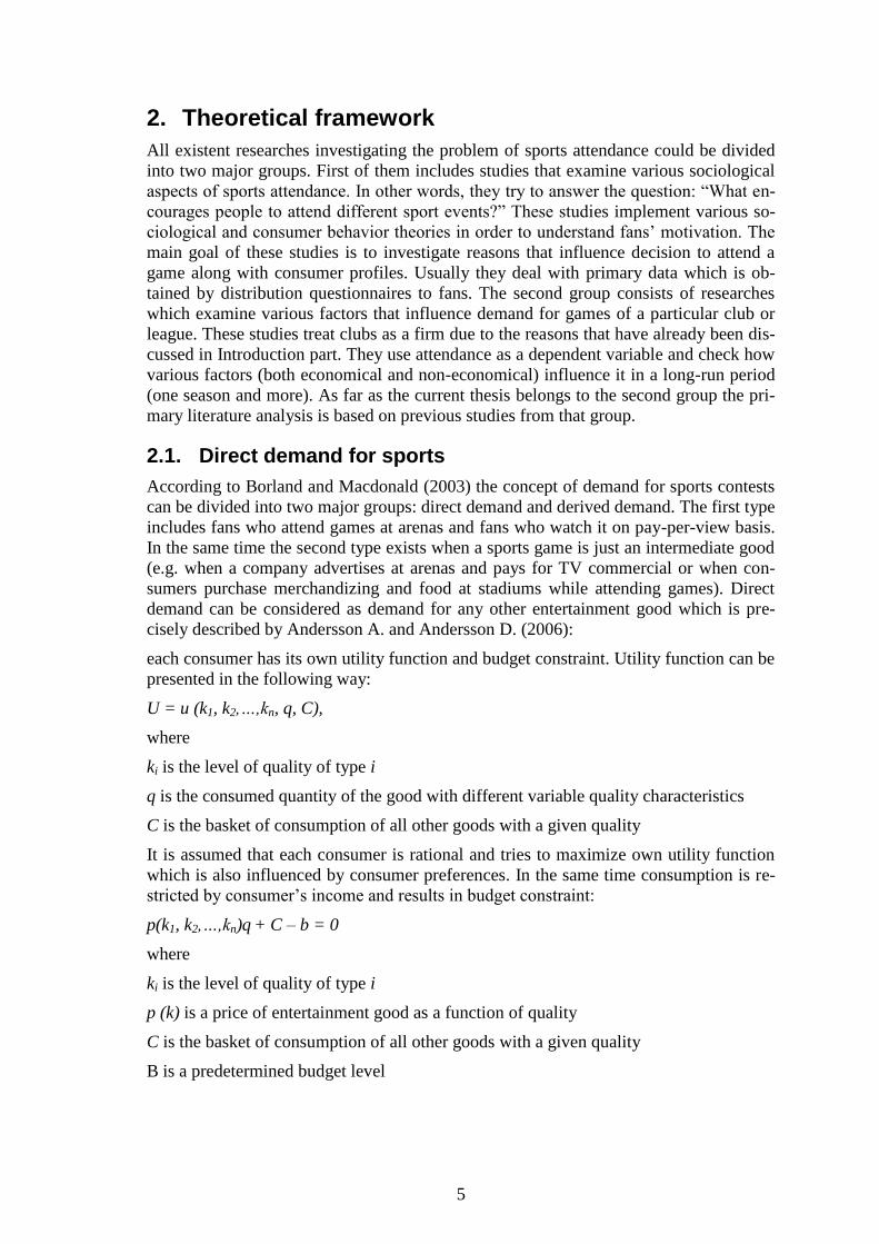
2.1. Direct demand for sports
According to Borland and Macdonald (2003) the concept of demand for sports contests
can be divided into two major groups: direct demand and derived demand. The first type
includes fans who attend games at arenas and fans who watch it on pay-per-view basis.
In the same time the second type exists when a sports game is just an intermediate good
(e.g. when a company advertises at arenas and pays for TV commercial or when con-
sumers purchase merchandizing and food at stadiums while attending games). Direct
demand can be considered as demand for any other entertainment good which is pre-
cisely described by Andersson A. and Andersson D. (2006):
each consumer has its own utility function and budget constraint. Utility function can be
presented in the following way:
U = u (k1, k2,…,kn, q, C),
where
ki is the level of quality of type i
q is the consumed quantity of the good with different variable quality characteristics
C is the basket of consumption of all other goods with a given quality
It is assumed that each consumer is rational and tries to maximize own utility function
which is also influenced by consumer preferences. In the same time consumption is re-
stricted by consumer‟s income and results in budget constraint:
p(k1, k2,…,kn)q + C – b = 0
where
ki is the level of quality of type i
p (k) is a price of entertainment good as a function of quality
C is the basket of consumption of all other goods with a given quality
B is a predetermined budget level

6
As a result a consumer has to select a set of goods which has maximum utility and is
limited by consumer‟s income. For simplicity it can be assumed that in case of ice
hockey games there are just two groups of goods: ice hockey games and other consump-
tion. Consequently a consumer faces a choice between attending an additional hockey
game at the stadium or instead of this spend income on additional unit of other goods
and services. This choice can be shown as a following graph:
Figure 2-1. Consumer choice (Andersson A. & Andersson D., 2006).
The number of goods a consumer can purchase depends on prices. If a price of one good
increases then a consumer reduces its consumption and in the same time slightly in-
creases consumption of another good. In case of ice hockey if ticket prices decrease
while the quality remains stable it will result in increase in consumption of ice hockey
games.
Figure 2-2. Changes in consumer choice (Andersson A. & Andersson D., 2006).
Consequently, demand for ice hockey games can be illustrated as a typical demand
curve with downward slope. Along with demand for any other good demand for ice
hockey games can be influenced by several factors (McConnell & Brue, 2008):
Tastes – if consumer preferences change and a good becomes more desirable
usually it leads to increase in demand. For instance, recent success of a national
team usually lead to higher attendance in local leagues. According to Allan
(2004) each victory of English national football team increases attendance of
the following Premier League games by 5.4 per cent.
Ice hockey games
Other consumption
Ice hockey games
Other consumption

7
Expectations – consumer expectations about higher future prices might also in-
fluence demand (one of the most intuitive examples is oil prices). Demand for
ice hockey is also influenced by future expectations. For instance, if fans see
that during pre-season a club strengthens squad they might expect better per-
formance during the season and higher demand for tickets. In order to avoid
queues and secure the best seats for the most interesting games they purchase
season tickets and as result have to attend even those games that they are less
interested in. Another example was observed in Europe during season
2004/2005. Due to lockout in NHL many top-star players moved to European
leagues in order to stay fit. As negotiations between clubs‟ owners and Players
Association were held during the whole season lockout could finish any day. In
this case NHL would have started which means that all star players would have
immediately gone back to North America and fans would not had an opportuni-
ty to watch them anymore so they tried to attend as many games as possible
what was one of the reasons for higher attendance across the whole Europe.
Substitute goods also have a strong impact on demand. Rise in prices for sub-
stitute goods leads to increase of consumption. In case of ice hockey lots of
substitutes can be taken into account from cinema and concerts to football and
other sports games. Existence of substitutes for ice hockey games and its actual
influence will be discussed more precisely in the next chapters.
Complement goods along with substitutes can also influence demand. If a price
for complement good rises (for instance, cars) it will lead to decrease in con-
sumption (in this case, car tires). Ice hockey games also have several comple-
ments: arena parking, public transportation, catering prices can influence fans
decision whether to attend a hockey game or not.
Number of buyers typically has an impact on demand. Migration to bigger cit-
ies increases demand for food and services in such metropolitan areas. Relation
between population and ice hockey attendance is usually positive though there
are some exceptions. It will be further investigated in the next chapters.
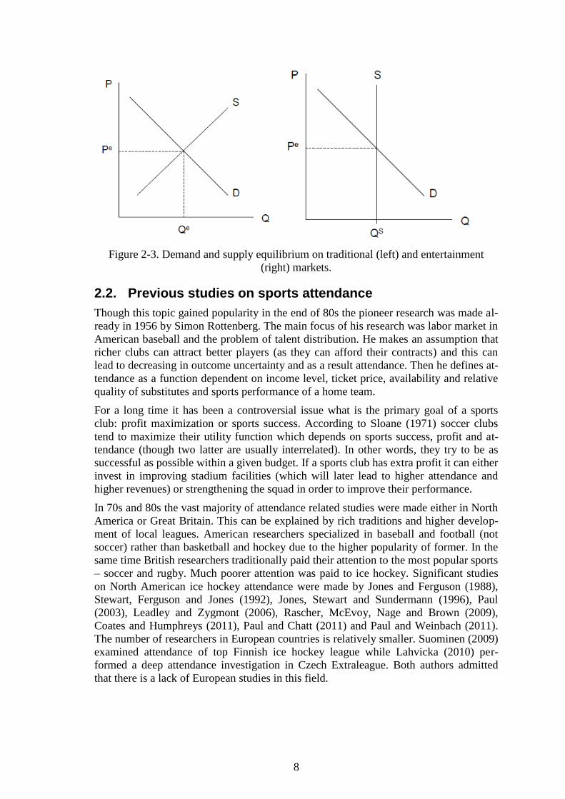
Demand and supply equilibrium for the majority of goods differs significantly from en-
tertainment goods (while ice hockey games are a part of them). Usually supply function
has upward slope and in case of increase (or decrease) in demand producers can modify
supply. One of the key features of sports games is that they are usually played at arenas
that have limited capacity. As a result supply function is a vertical line and no sports
club can influence it. The only thing they can do is just to renovate a stadium or play
some games at stadiums with bigger capacity. For instance, derby games between two
Stockholm based ice hockey clubs AIK and Djurgarden are played at Globen Arena
(capacity 13850) while other their home games are usually played at Hovet (capacity
8094).
8
Figure 2-3. Demand and supply equilibrium on traditional (left) and entertainment
(right) markets.
2.2. Previous studies on sports attendance
Though this topic gained popularity in the end of 80s the pioneer research was made al-
ready in 1956 by Simon Rottenberg. The main focus of his research was labor market in
American baseball and the problem of talent distribution. He makes an assumption that
richer clubs can attract better players (as they can afford their contracts) and this can
lead to decreasing in outcome uncertainty and as a result attendance. Then he defines at-
tendance as a function dependent on income level, ticket price, availability and relative
quality of substitutes and sports performance of a home team.
For a long time it has been a controversial issue what is the primary goal of a sports
club: profit maximization or sports success. According to Sloane (1971) soccer clubs
tend to maximize their utility function which depends on sports success, profit and at-
tendance (though two latter are usually interrelated). In other words, they try to be as
successful as possible within a given budget. If a sports club has extra profit it can either
invest in improving stadium facilities (which will later lead to higher attendance and
higher revenues) or strengthening the squad in order to improve their performance.
In 70s and 80s the vast majority of attendance related studies were made either in North
America or Great Britain. This can be explained by rich traditions and higher develop-
ment of local leagues. American researchers specialized in baseball and football (not
soccer) rather than basketball and hockey due to the higher popularity of former. In the
same time British researchers traditionally paid their attention to the most popular sports
– soccer and rugby. Much poorer attention was paid to ice hockey. Significant studies
on North American ice hockey attendance were made by Jones and Ferguson (1988),
Stewart, Ferguson and Jones (1992), Jones, Stewart and Sundermann (1996), Paul
(2003), Leadley and Zygmont (2006), Rascher, McEvoy, Nage and Brown (2009),
Coates and Humphreys (2011), Paul and Chatt (2011) and Paul and Weinbach (2011).
The number of researchers in European countries is relatively smaller. Suominen (2009)
examined attendance of top Finnish ice hockey league while Lahvicka (2010) per-
formed a deep attendance investigation in Czech Extraleague. Both authors admitted
that there is a lack of European studies in this field.

9
2.3. Fans’ categories
Though the majority of researchers used aggregate attendance in their studies some au-
thors made distinction between various groups of spectators. The key reason for this
distinction is that fan‟s decision to attend a game may be influenced by various factors
and thus should be considered separately. Although such separation might lead to more
accurate results it is usually neglected as this information is usually unavailable.
Season-ticket holders vs non-holders.
Forrest and Simmons (2002) admit that fans can be interested just in visiting more ex-
citing games but are afraid that they will not be able to purchase a ticket. That is why
they have to purchase a season ticket and visit even those games which are not attractive
to them. In the same time spectators who prefer single games would be more sensitive
to match specific factors.
Allan and Roy (2008) found that season-ticket holders‟ behavior is not affected by
game‟s characteristics and is relatively stable throughout the season. Moreover pay-at-
gate fans for some reasons can be even more important for the club as they are expected
to spend more on merchandizing and catering due to infrequency of visits comparing to
season ticket holders.
Home team vs away team fans
It is obvious that factors affecting attendance are different for home and away specta-
tors. Guest fans bear higher costs as they have to spend more money and time on travel.
Allan and Roy (2008) admit that visiting fans prefer games with lower win probability
of the home team.
Standing viewers vs seating viewers
This issue is typical for European clubs as arenas in North America usually have only
seating accommodation. Terraces (for standing audience) used to be extremely popular
in England but after Hillsborough disaster Football Association forced clubs to renovate
their stadiums. Nowadays standing seats can be rarely met at soccer arenas though ma-
jority of Czech, Finnish and Swedish ice hockey clubs still have terraces as a cheaper
option. Dobson and Goddard (1992) came to conclusion that attendance demand for
standing and seating accommodation is influenced by different factors. Current team
performance, game importance and rivalry have bigger influence on standings while
seated is more influenced by club‟s traditions.
2.4. Groups of factors
Based on Rottenberg‟s (1956) findings the majority of researchers divided all factors
which could influence attendance into four groups: economic aspects, expected quality,
opportunity costs and others. Garcia and Rodriguez (2009) also added uncertainty of
outcome factors to the model as this issue has become one of the major questions within
attendance related studies. Forrest and Simmons (2006) studied attendance in English
lower divisions and provided a more complicated model deriving several additional
groups of factors:
Support (previous season attendances, distance between clubs and rivalry)
Form (recent teams‟ performance)
Promotion contention (whether both teams are involved in promotion conten-
tion during different parts of season)
Outcome uncertainty

10
Television (if any games between best European clubs are televised in the same
time)
Schedule
Other dummies (month dummies and dummies for teams with greater support)
The only author who studied ice hockey attendance and implemented factors division
into groups was Lahvicka (2010). He derived five major groups of variables which are
similar to Rottenberg‟s approach:
Home team and season fixed effects
Match attributes (team quality/reputation; team form; team rivalry; team fresh-
ness/newness; match excitement/uncertainty; seasonal uncertainty; arena quali-
ty)
Economic and demographic factors (ticket price; population; distance between
home and away teams)
Substitution effects and opportunity costs (match day/time; TV broadcast;
weather; schedule congestion; substitution with other ice hockey teams; substi-
tution with soccer)
In the present paper a similar approach is used as all the factors are divided into five
groups: team effect variables, season effect variables, economic variables, match quality
variables and variables, which measure opportunity costs.
2.5. Economic factors
2.5.1. Price elasticity
Economic factors include those which are typical for any demand model: ticket prices,
prices of substitutes, area population where the club is based etc. The major obstacle in
calculating price elasticity is that sports clubs set differentiated prices for the same
game. Usually it depends on viewing quality (i.e. standing and seated; central lower and
upper corner levels etc.) and spectators‟ category (usually there are discounts for stu-
dents and seniors). Garcia and Rodriguez (2009) outline several possible solutions for
this problem:
Average ticket price ( e.g. Baimbridge, Cameron & Dowson, 1996)
Average price of sold tickets (total revenue is divided by the number of tickets
sold; e.g. Avgerinou & Giakoumatos, 2009)
Minimum ticket price (e.g. Garcia & Rodriguez, 2002)
Weighted average price (takes into account the tickets‟ total number of a cer-
tain price category; e.g. Benz, Brandes & Franck, 2009)
De Santana and Da Silva (2009) and Madalozzo and Villar (2009) studies on Brazilian
soccer attendance showed that clubs deliberately tend not to maximize profits but make
stadiums crowded. They admit that even if a club decides to increase admission price
the attendance will decrease slower as demand is inelastic at the point. This can be sup-
ported by majority of researchers (e.g. Allan, 2004; Bruggink & Roosma, 2003; Coates
& Humphreys, 2007 etc.) who also found demand to be inelastic. Madalozzo and Villar
(2009) concluded that even if a club gives 50 per cent discount on ticket prices sales
will increase just by 16 per cent. Moreover Simmons (1996) claims that pay-at-gate fans
have greater price elasticity comparing to season-ticket holders. Ice hockey clubs also

11
tend to keep demand in inelastic point which was supported by Suominen (2009) and
Lahvicka (2010) findings.
Clubs operate in inelastic point due to several reasons. Usually club revenues have sev-
eral other sources except gate revenues. Firstly, a club with a higher number of support-
ers is more attractive for advertisers and sponsors. Secondly, TV channels tend to select
for broadcasting those games which have lower number of empty seats in order to create
a unique atmosphere and as a result TV revenues are higher. Finally, supporters spend
money on merchandizing, catering and parking and as it was abovementioned casual
fans tend to spend more. So based on previous studies it follows that,
Hypothesis 1: The higher are ticket prices the less number of fans attend the game.
2.5.2. Population
Several researchers also analyzed the impact of population size on game attendance.
Falter and Perignon (2000), García and Rodríguez (2002), Paul (2003), Suominen
(2009), Paul and Chatt (2011) found a positive relationship between city population and
number of spectators. In the same time Paul (2003) admits that positive relationship ex-
ists only for Canadian teams in NHL while for American teams it is negative. Typically
just total city population is taken into account but Barajas and Crolley (2005) included
province population while Benz et al. (2009) used just male population considering men
to be the majority of spectators.
It is a typical situation for bigger cities to have more than one local club in the highest
division. For instance, this season London hosts 5 clubs of English Football Premier
League. As a result it can be challenging to calculate a number of people who reside in
the area of each club. It is possible to divide total population by the number of clubs but
Garcia and Rodriguez (2002) distributed it in accordance with the number of sold sea-
son tickets.
More complicated approach was implemented by Buraimo and Simmons (2006). Using
special software they constructed 5 and 10 miles concentric rings around each stadium
based on findings that loyal fans usually reside within 10 miles distance from arena.
They found that if a team has a population within 10 miles that is 100,000 greater than
another team, the team with larger population density is predicted to have 0.79 per cent
greater attendance. Difference in away team population of 100,000 translates into an in-
crease in attendance of 0.32 per cent.
Another interesting result was received by Lemke, Leonard and Tihokwane (2010).
They split the whole league data set into three groups based on city population. The
main result is that attendance of small market teams is much more sensitive to factors
surrounding the game and then is attendance of large market teams. They explained it
by the fact that in large markets a franchise has more season ticket holders or more peo-
ple to sell tickets to regardless of the game‟s characteristics. As a result, they came to
the conclusion that small market teams have to pay more attention to game characteris-
tics in order to increase demand for tickets.
Following these arguments it can be expected that,
Hypothesis 2: The bigger is population of a city the bigger number of fans attend a
game.

12
2.6. Expected quality
The second group of factors deals with expected quality of the game. Intuitively fans
prefer to see better performance and there are various approaches how to measure at-
tractiveness of every match.
2.6.1. Roster quality
One of the possible solutions to measure squad quality is to estimate teams‟ budget. It
can be assumed that teams with higher budgets can hire more skilled players and as a
result achieve bigger success. Falter and Perignon (2000) along with Garcia and Rodri-
guez (2002) used budgets of both teams and found a positive relationship between
budget and attendance. Though players‟ salaries usually are the biggest expenses of a
club sometimes it can be misleading. For instance, a team can spend a sufficient part of
its budget on improving training or stadium facilities during renovation period. As a re-
sult it can be more reasonable to use total team payroll as an indicator of team‟s roster
(Barajas & Crolley, 2005; Buraimo, 2008; Barilla, Gruben & Levernier, 2008). The lat-
ter found that in American baseball an increase in a team‟s player payroll of $10 million
attracts 610 more fans on average. As a team plays 81 home games per year a $10 mil-
lion investment in a team‟s payroll might increase total attendance by 49,400 fans.
Teams‟ wage bills can be interpreted not only in absolute figures but also in relation to
average payroll in league (Forrest, Simmons & Buraimo, 2005; Buraimo & Simmons,
2006, 2008; Di Domizio, 2010). A positive relationship between teams‟ payroll and at-
tendance exists though Buraimo (2008) found that home team wage bill is less im-
portant as it remains the same during the whole season. Moreover Mongeon and Win-
frey (2011) came to the conclusion that fans pay more attention to actual performance of
a team rather than to team's payroll.
Unfortunately data on team‟s budgets in Europe (especially in ice hockey) is not always
available so other proxies can be used to measure team‟s quality. Baimbridge et al.
(1996) along with Garcia and Rodriguez (2002) used a number of overseas players,
played in international game and found a positive relationship. In the same time re-
search on Brazilian soccer done by De Santana and Da Silva (2009) showed that exist-
ence of players with international experience is not significant for attendance demand.
It was already mentioned that fans prefer to watch best players so a bigger number of
superstars should increase attendance. The biggest obstacle is that usually it can be
problematic to measure this indicator credibly. Jones and Fergusson (1988) used a num-
ber of stars and found a positive relationship. The major disadvantage is that their as-
sessment was not based on any figures and was rather subjective. Stewart et. al. (1992)
used a number of selections to all-star team and number of players scoring more than 20
points. The same approach was implemented by Bruggink and Roosma (2003) and they
found that home stars are more important: every star brings 4.5 per cent increase com-
paring to 2.4 per cent by away star. The opposite result was obtained by Berri, Shmidt
and Brook (2004) as it turned out that team performance is much more important than
existence of stars in the roster. Brandes, Franck and Nuesch (2008) used a number of
top 2% highly paid players in the league and found that stars bring fans to the stadium
when they are on road (attendance increases by 4 per cent). This means that a team
spends money on star players though this does not influence home attendance but at-
tracts spectators when a team plays in another city. Nevertheless, it can be expected
that,

13
Hypothesis 3: The better is quality of a home team the bigger number of fans attends a
game.
Hypothesis 4: The better is quality of an away team the bigger number of fans attends a
game.
Hypothesis 5: The quality of away team roster is more important than the quality of
home team’s roster.
2.6.2. Teams’ league performance
Besides players in team‟s roster fans are definitely interested in team‟s performance.
There are various measures which can help to understand team‟s success. Due to the na-
ture of team sports, league standing might be the most important indicator of team‟s
success. Czarnitzki and Stadtmann (2002) found that there is a positive relationship be-
tween league position of both teams and attendance. Later Buraimo and Simmons
(2006) pointed out that performance of home team is more important comparing to
away team which was also confirmed by Lahvicka (2010). Moreover he admits that fans
pay much more attention to home performance than to away games. This means that if a
team is successful at home but loses away games it would have higher attendance than it
if it is equally average both at home and on road. In order to classify teams in the league
standing points are assigned according to game results. In order to measure team per-
formance usually average number of points per game is used. Results obtained by Paul
(2003), Forrest and Simmons (2006), Buraimo (2008) and Suominen (2009) confirmed
the previous assumption that fans pay more attention to home team performance rather
than to the opponents. The only problem is that in the first round every team has zero
points, so average number of points is also equal to zero. There are two possible solu-
tions: first round games can be excluded from the model or average number of points
can be taken from previous season.
It is evident that a team has to score as much as it can to win a game so fans should pre-
fer higher scoring teams. Results of Coates and Humphreys (2011) supported this as-
sumption while interesting results were obtained by Paul (2003). He analyzed attend-
ance in NHL and found that fans prefer teams that win and have tendencies towards
fighting and violence, as opposed to high-scoring, low-violence teams. Two later stud-
ies on minor American hockey leagues showed that in AHL fans value higher scoring
teams and they enjoy higher attendance (Paul & Chatt, 2011) but in QMJHL the number
of goals scored has no impact on the number of spectators (Paul & Weinbach, 2011).
All in all, it follows that,
Hypothesis 6: The better is league performance of a home team the bigger number of
fans attends a game.
Hypothesis 7: The better is league performance of an away team the bigger number of
fans attends a game.
Hypothesis 8: Performance of a home team in home games is more important than in
away games.
Hypothesis 9: Performance of a home team is more important than performance of an
away team.

14
Hypothesis 10: The bigger number of goals scores a team the bigger is the number of
fans who attend a game.
2.6.3. Latest team form
Apart from total league standing which represents how successful is a team during the
whole season short-term factors can also influence attendance. Due to various sports
and psychological reasons team performance may differ from month to month. Fans can
notice recent improvements and become more motivated to attend games. This indicator
can be highly significant: for instance, Iho and Heikkila (2010) found out that if a team
loses last five games instead of five wins it will lead to 31.6 per cent decrease in next
game attendance.
Overwhelming majority of researchers used the a similar approach to identify latest
team form: they took into account the total number of points gained in the last 3-5
games. Some of them (e.g. Garcia & Rodriguez, 2002; Benz et al, 2009) also introduced
an additional dummy variable if a team has a streak of several wins in a row. Everyone
except Allan and Roy (2008) found a positive influence of team form on game attend-
ance while in the latter study it turned out to be insignificant. Besides this, Czarnitzki
and Stadtmann (2002) along with Forrest and Simmons (2006) underline that home
team form is more important for fans in comparison with visitors. In European ice
hockey studies this trend was confirmed. Suominen (2009) found that Finnish fans were
not interested in the recent performance of a visiting team while Lahvicka (2010) con-
cluded that short-term results are more important than overall league position. Conse-
quently, it can be expected that,
Hypothesis 11: The better is latest home team’s form the bigger number of fans attends
a game.
Hypothesis 12: The better is latest away team’s form the bigger number of fans attends
a game.
Hypothesis 13: Recent form of a home team is more important than recent form of an
away team.
2.6.4. Violence
Violence factor has always been a controversial topic for ice hockey researches. Jones et
al. (1996) found fighting to be attractive for fans. Their study of NHL attendance
showed that in late 80s violence could become one of the tools to promote franchise.
However, they admit that there were significant regional differences. Canadian fans did
not want their team to fight though more violent visiting teams attracted higher audi-
ence. On the contrary, spectators in the US preferred teams with more aggressive play
style. Their findings were later confirmed by Paul (2003). He admits that on-ice vio-
lence is attractive for fans in both countries and for US teams coefficient is even higher
than for Canadian. Over the last decade North American leagues tried to reduce the
number of fights and recent studies showed that violence is not attractive anymore and
cannot increase attendance. Coates and Humphreys (2011) and Paul and Chatt (2011)
found negative influence of violence on the number of spectators. Paul and Weinbach
(2011) who examined attendance in QMJHL (arguably the best junior hockey league in
Canada and worldwide) state that such contradiction can be explained by Canadian pas-
sion for pure hockey without violence. Lahvicka (2010) also mentioned cultural differ-
15
ences and excluded this factor from his model as according to him fighting has never
been popular in Europe so it cannot be a determining factor in explaining attendance.
Following latest researches it can be expected that,
Hypothesis 14: There is no correlation between the number of fights and the number of
fans who attends a game.
2.6.5. Rivals
Games between historical and geographical rivals usually attract higher audience.
Sometimes results of these games can be even more important for fans than club's posi-
tion in the final standing. Usually these derbies arise between two neighboring clubs but
sometimes rivalry exists between historical opponents (for instance, El Clasico game
between Real Madrid and Barcelona in Spanish soccer). The majority of researchers in-
troduce dummy variable in order to capture this effect though selection principles are
different. Buraimo and Simmons (2008) assigned variable equal to one in case both
teams are from the same city or province. Forrest et al. (2005) estimated rivalry based
on their subjectivity. Lahvicka (2010) selected games as rival if travel time between two
cities is not more than 45 minutes.
Expectedly increase in number of fans is rather high: Forrest et al. (2005) found 7 per
cent improvement while Buraimo (2008) - 14.4 per cent. Moreover, Lahvicka concluded
that the main Czech derby between Sparta and Slavia (both teams are from Prague) at-
tracts 60 per cent more fans ceteris paribus. As a result it follows that,
Hypothesis 15: If both clubs are rivals it brings more fans to a game.
Hypothesis 16: If both clubs are from Stockholm it brings more fans than to any other
game between two rivals.
2.6.6. Short-term reputation
Successful clubs usually enjoy higher attendance not only at home but also when they
are on road. Fans can be expected to be more motivated to attend a game when one of
participants is a recent title holder. Researchers usually introduce dummy variable in
order to capture this effect. Allan (2004) found that every trophy won by a visiting team
leads to average increase in attendance by 0.88 per cent. Moreover, Madalozzo and Vil-
lar (2009) came to the conclusion that the effect is even greater if a visitor is a recent
champion. Soccer championships usually consist just of one stage while in ice hockey
regular season is followed by playoff round when champion is determined. Paul (2003)
noticed an interesting trend in NHL attendance. If a home team made playoff but lost in
the first round it has a negative influence on future season attendance which can be ex-
plained by fans‟ disappointment. In the same time qualifying for the second round has a
strong positive influence on future attendance. However, Lemke et al. (2010) admit that
a visiting team which was successful in the previous season attracts larger audience just
in the beginning of the season but after first two months this effect diminishes. A possi-
ble explanation is that in the middle of the season fans start valuing current team results
rather than past titles. Nevertheless, it can be expected that,
Hypothesis 17: If a home team secured the title last year the bigger number of fans at-
tends a game.

16
Hypothesis 18: If an away team secured the title last year the bigger number of fans at-
tends a game.
Hypothesis 19: If a home team made playoff last year the bigger number of fans attends
a game.
Hypothesis 20: If an away team made playoff last year the bigger number of fans at-
tends a game.
2.6.7. Long-term reputation
Recent team success and trophies won in a previous season can be a strong predictor of
current higher attendance. Besides this fans can be also attracted by clubs with strong
traditions and past success. A home team that achieved higher results in previous years
typically has a large number of loyal fans who continue supporting their favorite club
even in worse times. One of the most famous examples is a Spanish soccer club Atletico
Madrid. In 2000 it relegated from Spanish top division but fans were still devoted to
them and their attendance in the lower league was even higher than during the previous
year in elite. In a similar way clubs with strong traditions can attract large crowds when
they are on road. Russian soccer club Spartak Moscow has not won any national trophy
over the last ten years but still has the highest attendance among any other visiting
teams due to club‟s success both in Russia and Europe in 90s. Czarnitzki and Stadtmann
(2002) developed an indicator which allows to evaluate a long-term team reputation. It
is equal to
xt is the team's final ranking in the championship t years ago and n is the number of
teams in the first division.
In a similar way fans can be attracted not only by a well-known team but also by a new-
comer: a team which has never played in a top division before or is just promoted after
playing in a lower division. Lahvicka (2010) came to the conclusion that new teams at-
tract higher attendance both at home and on road while this novelty effect was equal to
8 per cent. Consequently, it can be expected that,
Hypothesis 21: The higher is reputation of a home team the bigger number of fans at-
tends a game.
Hypothesis 22: The higher is reputation of an away team the bigger number of fans at-
tends a game.
Hypothesis 23: If a home team has just promoted the bigger number of fans attends a
game.
Hypothesis 24: If an away team has just promoted the bigger number of fans attends a
game.

17
2.7. Uncertainty of outcome
Uncertainty of outcome is one of the most debated issues in sports attendance studies.
The core idea is based on assumption that close games (when difference in teams
strength is minimal) should attract more spectators due to uncertainty of the final result.
Garcia and Rodriguez (2002) following previous studies suggested distinguishing be-
tween season and match uncertainty as these factors can influence attendance in a dif-
ferent way.
2.7.1. Playoff, season uncertainty
Fans are interested not just in a win of their favorite team in a particular game but in
overall club's success based on the whole season as well. There are several basic ap-
proaches how to measure season uncertainty. Baimbridge et al. (1996) introduced sev-
eral dummy variables equal to 1 if a team is from top-4 or low-4 clubs (which means
that a team battles for the title or avoiding relegation). He found that relegation leads to
fans' frustration and sharply decreases attendance. Similar methods were also used by
other researchers:
Garcia and Rodriguez (2002) used a dummy variable when a team lost chances
to win championship or avoid relegation. According to them, attendance rapid-
ly decreases when season outcome becomes clear for fans.
Forrest and Simmons (2006) took into account top-6 teams and found that there
was a significant positive relation between uncertainty and game attendance.
Madalozzo and Villar (2009) came to the conclusion that attendance increases
if a team still keeps chances for winning the title or avoiding relegation.
According to Iho and Heiikila (2010) attendance of insignificant matches
(those when no team still battles for a better position to qualify for European
competitions or avoid demotion) is 13.6 per cent lower.
A more complicated measure was used by Czarnitzki and Stadtmann (2002). They in-
troduce a special variable U:
where c denotes to the points needed to win championship, b the number of points a
team already has and t the number of games already played, m is the maximum number
of points a team can collect during the season.
The major disadvantage of this approach is that it can be measured properly just after
the end of the season. Before its finish no one can calculate how many points a team
needs to become a champion.
Ice hockey studies rarely took this factor into account. One of the possible explanations
is that a champion is determined during playoffs that is why regular season is less im-
portant. Majority of teams usually keep chances to qualify for playoffs until the end of
the season as usually more than a half of the teams reach it. Paul (2003) used a dummy
variable for games during the last two months of regular season as they have larger im-
pact on identifying teams which are qualified for playoffs. Much more complicated
18
method was implemented by Lahvicka (2010). Using Monte-Carlo simulation he simu-
lated possible results of each game and based on that calculated winning probabilities
and as a result reaching playoffs or avoiding relegation. Finally, he came to the conclu-
sion that attendance sharply decreases as a team loses chances to participate in playoffs
or avoid relegation to the lower division. In the same way, it can be expected that,
Hypothesis 25: If there is no season uncertainty the smaller number of fans attends a
game.
2.7.2. Match uncertainty
Defining match uncertainty could be even a more difficult task. All approaches used in
previous studies can be divided into two groups: results in current championship and
betting odds.
Difference in league positions
Baimbridge et al. (1996) found no evidence of influence on attendance while
Benz et al. (2009) came to the conclusion that if a difference between teams'
positions increases by 1 point then attendance decreases by 1.6% per cent.
Squared difference of league positions
Garcia and Rodriguez (2002) received mixed results. On the one hand, a low
difference increased attendance (this confirms assumptions that fans can be at-
tracted by games where both teams are almost equal) but on the other hand, if
an away team was much higher in the league table than a home team attend-
ance also increased.
Points difference
De Santana and Da Silva (2009) used simple difference in points gained by the
date of the match but found this factor to be insignificant. This approach can
lead to biases as close to the end of the season this difference can be quite suf-
ficient though teams can occupy next positions in the league table.
Positions in the league standing
Jones et al. (1996) used a dummy variable if both teams were from top-3 and if
one team was from top-3 and another was from bottom-3. The former coeffi-
cient turned out to be significant unlike the latter. This method also has a dis-
advantage as higher attendance of games involving teams from top-3 can be in-
fluenced by a range of other factors (e.g. star players and expectations of high-
class performance). In the same time, a game between both teams which occu-
py positions in the middle of league table can also be uncertain.
Home prospects
More complex approach was introduced by Forrest et al. (2005) when analyz-
ing factors which can influence TV-audience watching soccer games. They
measure game uncertainty as „„home advantage plus points-per-game to date of
the home team minus points-per-game to date of the visiting team, where home
advantage is equal to mean points-per-game by all home teams in the previous
season minus mean points-per-game by all away teams in the previous season.
The same method was later used by Buraimo (2008) who found it to be insig-
nificant.
Probability of dramatic game
Lahvicka (2010) used another approach to measure uncertainty. He calculated
a special variable called "drama probability" and constructed a model to predict

19
final result of each game. If there was an evidence that difference in goals
scored by both teams is not more than one it can be attractive for fans (if there
is a draw then teams will play overtime while if difference is equal to one then
one team can pull a goalkeeper and substitute him with additional player in or-
der to score equalizer). He came to the conclusion that match uncertainty has a
positive impact on attendance.
Betting odds
Some could think that betting odds might be a good predictor of each team
chances to win and as a result it could be a measure of outcome uncertainty.
Despite of this Forrest and Simmons (2002) found that betting odds can pro-
vide biases as sometimes bookmakers provide superior returns when betting on
underdogs and less supported teams. Nevertheless, results of Buraimo and
Simmons (2009) study showed that match uncertainty has insignificant influ-
ence on attendance. Moreover, they admit that Spanish soccer fans tend to pre-
fer games with high (when fans are sure that team will win) or low (when a
strong opponent is coming) probability of home team win.
Even though previous results are mixed it can be expected that,
Hypothesis 26: The higher is game uncertainty the bigger number of fans attends a
game.
2.8. Opportunity costs and other factors
2.8.1. Day of the week
Visiting a game is a similar leisure activity as any other. As people usually have less lei-
sure time on weekdays it should have a significant impact on attendance. The majority
of studies found attendance to be lower during midweek (e.g. Allan, 2004; Forrest &
Simmons, 2006) while on weekend the number of spectators is higher by 10 per cent on
average (Suominen, 2009; Lahvicka, 2010). Christmas and public holidays when people
typically prefer to go out attract even bigger number of spectators from 14 per cent (Al-
lan, 2004) to 20-23 per cent (Lahvicka, 2010) more. It follows that,
Hypothesis 27: If a game is played on Friday the bigger number of fans attends it than
if it is played on a weekday.
Hypothesis 28: If a game is played on Saturday the bigger number of fans attends it
than if it is played on a Friday.
Hypothesis 29: If a game is played during Christmas holidays the bigger number of fans
attends it than if it is played on a Saturday.
2.8.2. Opening night
Ice hockey season in North America starts in October and finishes in June. European
leagues usually start in September and finish in April so fans do not have an opportunity
to see their favorite team during 4 or 5 months. Of course they can attend pre-season
games in August but these matches are used for improving player's form, try new tactics
and do not have any importance that is why they are called "friendly" games. As a result
fans have to wait for the start of the season and first game attracts larger audience. Ac-

20
cording to Lahvicka (2010) first games have 9 per cent higher attendance but Coates
and Humphreys (2011) found that opening night attracts 22 per cent spectators more
than other games of the season. In the same time, Paul (2003) admits that even though
attendance of the first match is significantly higher next games have smaller audience as
the quality of hockey is relatively low and season uncertainty is not so high. Moreover,
in the US the most important football and baseball games are played in autumn so this
can also decrease ice hockey attendance. Consequently, it can be expected that,
Hypothesis 30: If a game is the first home match of the season the bigger number of
fans attends it.
2.8.3. Series of home games
Game schedule in top soccer leagues is organized in a way that a team plays one game a
week at home and the next week on road. In lower divisions sometimes teams have to
play two consecutive games at home. As a result, fans might prefer to attend just one
match out of two which reduces attendance. Forrest and Simmons (2006) found that
fans usually prefer to visit the first game. Ice hockey schedule is slightly different and
sometimes teams play two, three or even four games in a row at home. Probably this
could influence attendance in a negative way especially if interval is relatively short.
Lahvicka (2010) estimated that if there is just one day between two consecutive games
at home then attendance is 2 per cent lower for the first game and 4 per cent lower for
the second. It follows that,
Hypothesis 31: The smaller is the break between two consecutive home games the
smaller number of fans attends a game.
2.8.4. Distance
As it has already been mentioned attendance of a particular game consists not only of
home spectators but also of visiting team supporters. Away team fans face higher op-
portunity costs as they have to spend more time and money to get to another city. As a
result if a distance between two cities is smaller a higher number of visiting fans can be
expected. The majority of previous studies (e.g. Forrest & Simmons, 2006; Allan &
Roy, 2008; Buraimo, 2008) used two variables in order to estimate this effect – distance
in kilometers and distance squared. Benz et al. (2009) substituted distance with travel
time obtained from Deutsche Bahn (German Railways) website as the majority of fans
use trains to reach another city. Some German clubs even combine train and game tick-
ets thus giving their fans a sufficient discount. Expectedly, distance has a negative im-
pact on attendance as it reduces the number of away fans and decreases rivalry. As a re-
sult, it can be expected that,
Hypothesis 32: The less is the distance between two teams the bigger number of fans at-
tends a game.
2.8.5. Substitution with other clubs
Sports game is not similar to any other good. In case there are two teams from the same
city, fans do not choose which game to attend. They have their own favorite team and
will not go to see another team's game. Lahvicka (2010) came to the conclusion that two
teams from the same city are poor substitutes. In the same time, if there are two clubs
from the same province it can lead to higher attendance due to increasing rivalry. Breuer
(2009) found that if an additional club from the same city enters the league it leads to

21
higher ticket sales for both clubs due to raise of interest towards soccer in the city.
However, it is a quite common situation when there are two sports clubs in the same
city, for instance soccer and an ice hockey. As a result, some fans cannot afford support-
ing both teams and have to make their choice. Existence of a soccer club in the same
city results in 5 per cent decrease in attendance. So it can be expected that,
Hypothesis 33: If there is a football or an ice hockey game in the same day in the same
city the number of fans who attends a game will be smaller.
2.9. Team and season variables
Previous chapters described a great deal of factors that influence sports attendance.
Nevertheless, there are some trends that cannot be captured by any abovementioned var-
iable. Specific team‟s or season‟s variable were rarely used in previous studies. Lah-
vicka (2010) introduced a special dummy variable for each team that was included in
the dataset. According to him, this variable describes such factors as overall level of
team popularity, quality and capacity of the arena. Besides this, he also used a season
variable that can help to capture changes in rules and other factors that change only
once a season (for instance, a national team might win a World Cup or Olympic games
and that led to raise of ice hockey popularity across the country). Later a similar ap-
proach was implemented by Paul and Weinbach (2011). They introduced dummy varia-
ble for each home and away team and found that some teams are much popular both at
home and on road. Based on these arguments, it can be expected that,
Hypothesis 34: Every team has its own base attendance.
Hypothesis 35: Attendance is influenced by a respective season effect.
22
3. Method
The analysis is conducted using quantitative methods, where econometrical and statisti-
cal approaches are primary tools. In order to test factors influencing the attendance a
multiple regression model was set up.
Regression analysis helps to understand how the typical value of dependent variable
changes when any independent variable is varied, while other independent variables are
held fixed. The regression analysis is widely used for prediction and forecasting and al-
so used to understand which independent variables are related to dependent variable and
to explore the forms of these relationships (Archdeacon, 1994). Therefore, it is the most
appropriate method to reveal which factors commonly affect attendance of hockey
games. Moreover, using regression techniques allows predicting future attendance and
changing ticket prices and promotion strategies based on this knowledge. To estimate
the parameters of the regression ordinary least squares (OLS) method was used. IBM
SPSS Statistics software package version 19 was used to calculate the regression.
The model can be summarized in this equation: ln (match attendance) = f (home team
effects, season effects, match quality attributes, economic factors, and opportunity
costs) + error term
In total, there are 61 independent variables in the model (home team effects: 13 varia-
bles; season effects: 3 variables; match attributes: 29 variables; economic factors: 2 var-
iables; opportunity costs: 14 variables).
3.1 Data Collection
The dataset is compiled using secondary data and consists of 1320 regular season ice
hockey matches played during 4 seasons (from 2008/2009 to 2011/2012) in the top
Swedish ice hockey league called Elitserien. Three fixtures were excluded from the
model due to their specific nature. These games were played outdoor, therefore they ex-
cited public more than any other game and attendance was not affected by arenas‟ ca-
pacities. Therefore, the model consists of 1317 observations from 4 latest seasons. Pre-
vious seasons are also used to construct lagged team reputation variable. The main
sources for compiling the dataset are game reports provided by Swedish Ice Hockey As-
sociation and Elitserien. The data is collected and provided by official authorities, which
organize the competition.
The number of players participated in Olympic Games and World Championships along
with the number of the players, who have played in NHL, was derived from the official
information provided by the organizers of these competitions: International Olympic
Committee, International Ice Hockey Federation and National Hockey League respec-
tively. The source of city population was Swedish Statistical Bureau (Statistiska cen-
tralbyrån). The web-service ViaMichelin were used to calculate distances between cit-
ies.
Ticket prices are obtained by examining clubs‟ websites, internet ticket merchant
www.ticnet.se and provided by clubs‟ management, when data was not available from
public sources.

23
3.2 Delimitations
Multiple regression analysis creates a possibility of developing a wrong model or wrong
model interpretation, including statistically insignificant factors or rejection of statisti-
cally significant factors as well as problems of autocorrelation and multicollinearity, etc.
These problems might reduce the predictive power of the model or make it inappropri-
ate. According to Studenmund (2006), to avoid and solve these problems statistical
tests, such as t-test, F-test, variance inflationary factor should be carried out. The results
of the tests facilitate to choose an appropriate and reliable model.
The analysis of Elitserien puts certain limits to use it for other hockey leagues, since it is
located in a specific socio-geographic area with certain consumer habits and prefer-
ences. Moreover, playoff games were not included in the analysis because these games
are influenced by other factors and have different rules of competition, so authors do not
intend to discuss them in this paper.
3.3 Variables
The purpose of the analysis is to investigate which factors have influence on game at-
tendance. In order to test this, a linear regression model is set up and an OLS regression
is run. The dependent variable in the model is “Attendance”. A natural logarithm of the
officially registered number of spectators who visit each particular game was used in
order to address issues with its raw distribution.
All independent variables which affect attendance are divided into 5 groups: team effect
variables, season effect variables, economic variables, match quality variables and vari-
ables, which measure opportunity costs.
The match quality variables mainly describe sports characteristics of a team. This group
includes: “HomeTeamHomePoints”, “HomeTeamAwayPoints”, “HomeTeamGoals”,
“AwayTeamHomePoints”, “AwayTeamAwayPoints‟, “AwayTeamGoals”. These varia-
bles depict the average number of points/goals per game gained by home/away team at
home or on road from the start of the season. For the first game of each season the value
was obtained from the previous season. The maximum number of points, which a team
can get in one game is 3, the minimum is 0. Data sources were official reports from
each game of the Elitserien.
“MatchUncertainty” variable is related to previous variables. It is measured as home
advantage plus average number of points of the home team minus average number of
points of the visiting team, where home advantage is equal to average points of all home
teams in the previous season minus average points gained by all away teams in the pre-
vious season.
“LastFormHome” and “LastFormAway” variables were calculated by summing up
number of points gained by home/away team in the last 5 matches prior to a current
game. These variables range from a minimum 0 (denoted 5 straight loses in the regular
time in the last 5 matches) to a maximum 15 (denoted 5 straight wins in the regular time
in the last 5 matches). Variables were recalculated for each observation.
“HomeReputation” and “AwayReputation” variables imply long-term sports perfor-
mance of the team. The variables are calculated using the following formula:

24
, where T=5, xt - is the team's final ranking in the championship t years ago and n - is
the number of teams in the first division. The minimum value, which is 1,68 was ob-
tained by the number of teams, which promoted to Elitserien in the reviewed period.
“HomeFights” and “AwayFights” variables describe an average number of fights per
game from the start of the season.
“HomeChampion” and “AwayChampion” dummy variables describe whether a home or
an away team won the previous season Playoffs (Slutspel); “HomePlayoff”,
“AwayPlayoff” whether a home/away team was qualified for the previous season
Playoffs; “HomePromoted”, “AwayPromoted” if a home/away team was delegated from
the lower league Allsvenskan to Elitserien for a current season. If the answer for above
mentioned questions is yes, then variables take the value 1, in the other cases – 0.
“HomeNoQualify” and “AwayNoQualify” dummy variables describe the possibility of
a team to participate in the upcoming Playoffs. If a team lost a chance to qualify for the
Playoffs, the value is 1, if not - 0.
The number of players participated in Olympic Games and World Championships along
with the number of the players, who have played in NHL, was derived from the official
information provided by the organizers of these competitions: International Olympic
Committee, International Ice Hockey Federation and National Hockey League respec-
tively. “HomeOlympics” and “AwayOlympics” variables include the number of players,
who have played at least 5 games in men‟s ice hockey tournaments at Olympic Games.
The variables “HomeWC” and “AwayWC” include the number of players, who have
played at least 20 games in men‟s ice hockey World Championships. The variables
“HomeNHL” and “AwayNHL” include the number of players, who have played at least
200 games in National Hockey League.
“StockholmRival” dummy variable describes games between two Stockholm-based
teams: AIK and Djurgarden. The variable takes 1, when AIK and Djurgarden were play-
ing against each other, and 0 for all other games. It should be mentioned, that those
games were played in the most capacious ice hockey arena in Stockholm, Globen.
Whereas other games are played in the Hovet, which capacity is almost 6,000 seats less.
Therefore, there is no surprise that Stockholm‟s derby attracts more than 10,000 specta-
tors every game. The dummy variable “Rival” describes geographical derbies. The vari-
able takes 1, when the distance between cities is less than 150 km, and 0 for all other
games. The variable takes 0 for games between AIK and Djurgarden as well.
The group of economic variables includes “Population” and “Price”. The variable “Pop-
ulation” describes the number of inhabitants living in the city, where each hockey team
is based. The source of the data is the Swedish Statistical Bureau (Statistiska central-
byrån).
The variable “Price” is the natural logarithm of average ticket price for an adult person.
The logarithm was used due to the raw distribution. The value was calculated for each
team once a season. If a team implemented variable pricing the value was calculated for

25
each game. Price sources were clubs‟ websites, management and internet ticket mer-
chant www.ticnet.se.
The third group of variables describes opportunity costs.
“Opening Night” dummy variable is used for the first games at home for each team at
the start of each season. The variable takes 1 if the game is the first at home for a team,
and 0 if not.
“Friday”, “Saturday” and “Sunday” dummy variables describe the day when the game
was held. If the game was played on Friday, Saturday or Sunday the variable takes the
value 1, while the others take 0 respectively. When the game was played on weekday,
all the variables are equal to 0.
“Break” variable describes a number of days between two consecutive home games of
each team. The minimum value for the variable is 1, when the team has 1 day break be-
tween two home games; the maximum is 24. There were no home games played in two
consecutive days. For the first games of each season the variable takes the value of the
longest break during the season, since the opening night has the longest break from the
previous game by nature, but using 6-monts break is not rational to understand the sig-
nificance of this factor.
“Christmas” dummy variable is used to specify games played during Christmas holi-
days. The variable takes 1 if the game were held during this period and 0 if not.
Dummy variables “September”, “October”, “November”, “December”, “January”,
“February” and “March” describe the month when the game was held. If the game was
played in September, October, November, December, January, February or March the
variable takes the value 1, while the others take 0 respectively. The variable "Septem-
ber" is a reference variable and is omitted from the model.
A distance between two team-based cities is described by the variable “Distance”. The
value of the variable is calculated using web-service ViaMichelin, which provides data
for road distance between team-based cities in kilometers.
The variable “Football” is a dummy variable and takes the value 1 in two cases. Firstly,
if a hockey team played at home on the same day as a football club from the same city
played at home as well. Secondly, if any hockey team played on the same day as Swe-
dish men‟s national football team played official match irrespective home or away.
There were 23 games that fulfill the condition. National football games intersected ice
hockey games 4 times in Octobers 2008, 2009, 2010, 2011, affected totally 13 games.
Other 10 matches were affected by football teams played in the same time in Stock-
holm, Gothenburg and Gavle. For all other observations the variable takes 0.
Several variables were introduced to depict fixed effects of each seasons and teams. The
dummy variables "Season 0809", “Season0910”, “Season1011”, “Season1112” denote
the date when the game was played. Elitserien regular seasons was scheduled from Sep-
tember to March, therefore, if the game was held from September 2008 to March 2009
the value of “Season0809” is 1, “Season0910”, “Season1011 and “Season1112” is 0.
The same rule applies for the season 2009/2010, 2010/2011 and 2011/2012. The varia-
ble "Season 0809" is a reference variable and is omitted from the model.

26
Dummy variables “AIK”, “Brynas”, “Djurgarden”, “Farjestad”, “Frolunda”, ”HV71”,
”Linkoping”, ”Lulea”, ”Modo”, ”Rogle”, ”Skelleftea”, ”Timra” and ”Vaxjo” describe a
home team of each game and is equal to one for all home matches of a particular team.
The variable "Sodertalje" is a reference variable and is omitted from the model.

27
4. Results
4.1. Attendance
The minimum number of spectators was 2424 at Sodertalje – Rogle game, the maxi-
mum was 13850 at several games between AIK and Djurgarden. The least attended club
during last 4 years is Sodertalje SK with an average 3900 spectators at each home game.
The most attended club is Frolunda with 10441 spectators on average. HV has the most
stable audience, which fluctuates from 6526 to 7038 visitors per game. The most unsta-
ble club in terms of attendance is AIK. Their difference between minimum and maxi-
mum level of spectators is more than 10.000. The average attendance in the league is
6221 spectators per game.
Chart 4-1. Match attendance, descriptive statistics
Team Minimum Mean Maximum Standard
Deviation
AIK 3153 5531 13850 2373
Brynas 3978 5950 8538 1213
Djurgarden 3319 7075 13850 1630
Farjestad 5125 6605 8583 933
Frolunda 7501 10441 12044 1271
HV 6526 6894 7038 149
Linkoping 5365 6983 8500 876
Lulea 3857 5166 6300 549
Modo 4852 6309 7600 777
Rogle 3223 4497 5095 506
Skelleftea 3891 5066 6001 564
Sodertalje 2424 3900 6189 812
Timra 3612 4997 6000 593
Vaxjo 4406 5099 5502 290
Total 2424 6221 13850 1873
4.2. Model summary
The model is significant at 99% level according to F-test, which means that results are
trustworthy and might be applicable. Coefficient of Determination is 0,833, therefore 83
per cent of total variation in attendance is explained by variation in the chosen inde-
pendent variables. It is a quite high value (especially comparing to previous similar
studies), sustaining the applicability of the model.
Another important characteristic of the model is the Durbin-Watson statistic. This indi-
cator measures how a dependent variable correlates in time regardless of influence of
factors. In our model DW statistic has value 1.444, which is close to 2. It means that the
model is not autocorrelative and OLS can be applied to estimate coefficient of determi-
nation of this model.

28
The variance inflation factor (VIF) describes multicollinarity between independent vari-
ables. High value of this index indicates that factors in the model are highly correlated
between themselves, which leads to biased estimation of the coefficients. In our case
just a few variables have VIF higher than critical value 5. They are Home WC, Home
NHL, Home Reputation, Price and some team effect variables. The reason is that team
fixes factors already take into account influence of above-mentioned variables.
Chart 4-2 presents coefficients for the model and effect of each variable. The coeffi-
cients are unstandardized, which means that the magnitude of their values is relative to
means and standard deviations of independent and dependent variables in the equation.
Coefficients show amount of change in the dependent variable (Attendance) that is as-
sociated with change in one unit of the independent variable. Since the dependent varia-
ble is a natural logarithm, it is not easy to interpret an effect of each factor to attend-
ance, therefore the column “Effect” was added. To estimate the effect of a variable the
constant e was raised to the power equal to the value of coefficient. The column effect
shows the percentage changing attendance by changing each particular variable by 1
unit. The effect for the variable “Distance” is calculated per each 100 kilometers, for the
variable “Population” for each 10.000 inhabitants. The effect of price is equal to coeffi-
cient because this variable was already logged. Team effects were calculated by adding
the team coefficients to the constant and raised to the power. The constant itself might
be interpreted as a fan base for Sodertalje in September 2008. It can be easily checked
by running an OLS regression with the dummy variable Sodertalje, excluding the con-
stant. All the variables will have the same coefficients, while the variable Sodertalje will
take the value of "Constant" equal to 7,298. Therefore, team effects show basic number
of home games visitors by September 2008.

29
Chart 4-2. Estimation results
Variables Coefficient Effect Variables Coefficient Effect
Team effect variables Match Quality variables
AIK 7,487*** 1 785 HomeTeamHomePoints 0,004 0,44%
Brynas 7,673*** 2 150 AwayTeamAwayPoints 0,009 0,89%
Djurgarden 7,799*** 2 438 HomeTeamAwayPoints 0,004 0,39%
Farjestad 7,737*** 2 291 AwayTeamHomePoints 0,025** 2,50%
Frolunda 8,178*** 3 561 HomeTeamGoals 0,041*** 4,15%
HV71 7,702*** 2 214 AwayTeamGoals -0,011 -1,10%
Linkoping 7,832*** 2 520 MatchUncertainty 0,007 0,74%
Lulea 7,602*** 2 001 HomeForm 0,006*** 0,59%
Modo 7,699*** 2 206 AwayForm -0,002 -0,18%
Rogle 7,420*** 1 669 StockholmRival 0,806*** 123,83%
Skelleftea 7,528*** 1 860 Rival 0,101*** 10,68%
Sodertalje 7,298*** 1 478 HomeChampion 0,029 2,91%
Timra 7,549*** 1 898 AwayChampion -0,011 -1,08%
Vaxjo 7,491*** 1 791 HomePlayoff 0,003 0,30%
Season effect variables AwayPlayoff -0,013 -1,26%
Season0910 -0,037** -3,65% HomePromoted 0,045Ɨ 4,58%
Season1011 -0,048*** -4,65% AwayPromoted 0,001 0,13%
Season1112 -0,024 -2,41% HomeOlympics 0,008 0,84%
Opportunity costs variables HomeWC 0,009 0,88%
OpeningNight 0,104*** 10,98% HomeNHL -0,001 -0,09%
Friday 0,05* 5,18% AwayOlympics 0,013* 1,29%
Saturday 0,096*** 10,08% AwayWC -0,013*** -1,27%
Sunday 0,016 1,62% AwayNHL 0,002 0,24%
Christmas 0,103*** 10,90% HomeNoQualify -0,121*** -11,43%
Break 0,002** 0,24% AwayNoQualify -0,003 -0,25%
October 0,053** 5,43% HomeReputation 0,007Ɨ 0,71%
November 0,053** 5,43% AwayReputation 0,004** 0,45%
December 0,017 1,68% HomeFights 0,314** 36,92%
January 0,04* 4,09% AwayFights 0,246* 27,85%
February 0,074*** 7,69%
March 0,12*** 12,75% Overall Model F 102,283***
Football -0,065* -6,33% R Square 0,833
Distance -0,001*** -0,42% Adjusted R Square 0,824
Economic variables Std. Error 0,119
Population 0,001** 0,04% Durbin-Watson 1,444
Price 0,129** 12,9% N=1317; Ɨp<0.1; **p<0.05; **p<0.01; ***p<0.001

30
4.3. Hypothesis testing
All independent variables which affect attendance are divided into 5 groups: team effect
variables, season effect variables, economic variables, match quality variables and vari-
ables, which measure opportunity costs. 35 hypotheses on ice hockey attendance in
Sweden were tested.
Higher ticket prices do not lead to smaller number of fans attending the game. Quite the
contrary, the higher are ticket prices the greater number of fans attend the game (b=
0.129, p<0.01). Therefore hypothesis 1 is rejected.
The bigger is city population the bigger number of fans attend a game (b=0.001,
p<0.01). It fully supports hypothesis 2.
Roster quality characteristics of home team itself have a small correlation with attend-
ance (r=0.335, r=0.465, r=0.248, p<0.001) and are not significant in the model. Howev-
er, characteristics of away team roster are more significant (b=0.013, p<0.01 and b=-
0.013, p<0.001) Therefore hypothesis 3, 4 and 5 are partly confirmed.
Performance of a home team in both home and away games is slightly correlated with
attendance (r=0.182, r=0.148, p<0.001) and not significant in the model. Thus, hypothe-
sis 6 is partly confirmed and hypothesis 8 is supported. The performance of an away
team is significant in the model (b=0.025, p<0.01), therefore hypothesis 7 is supported
and 9 is rejected. Hypothesis 10 is fully supported for a home team (b=0.041, p<0.001)
Hypothesis 11 is confirmed (b=0.006, p<0,001), hypothesis 12 is rejected, since there is
no significant correlation between latest away team form and attendance. Thus, hypoth-
esis 13 is fully supported.
Fights have a significant impact on attendance. Both, average number of home team's
fights and away team's fights are important (b=0.314, p<0.01 and b=0.246, p<0.05).
Therefore, hypothesis 14 is rejected.
Hypothesis 15 and 16 are supported both for rivalry (b=0.101, p<0.001) and Stockholm
rivalry (b=0.806, p<0.001).
Home team title and making playoffs in a previous season have a positive correlation
with attendance (r=0.133, p<0.001 and r=0.321, p<0.001), however are insignificant in
the model. Thus hypothesis 17 and 19 are partly supported. Hypothesis 18 and 20 for an
away team are not significant at all and rejected.
Hypothesis 21 and 22 are confirmed for home (b=0.007, p<0.1) and away teams
(b=0.004, p<0.01).
Hypothesis 23 for home team, which has just promoted is confirmed (b=0.045, p<0.1),
hypothesis 24 for away team is rejected since there is no significant correlation between
attendance and newly promoted away team.
Team's possibility to qualify for the Playoffs is significant (b=-0.121, p<0.001), there-
fore hypothesis 25 is supported.
Match uncertainty is insignificant in the model and has a slight correlation with attend-
ance (r=0.125, p<0.001). Hypothesis 26 is partly confirmed.

31
Public prefer to attend games on Saturday (b=0.096, p<0.001) more than on Friday
(b=0.05, p<0.05). The biggest impact, meanwhile, has a Christmas break (b=0.103,
p<0.001) Thus, hypothesis 27, 28 and 29 are supported.
The relation between attendance and the first home match is positive and significant
(b=0.104, p<0.001), that supports hypothesis 30.
The greater is a break between two consecutive home games the bigger number of spec-
tators will attend a game (b=0.002, p<0.01), that supports Hypothesis 31.
Bigger distance decreases the number of spectators (b=-0.001, p<0.001), therefore hy-
pothesis 32 is confirmed.
There were no clashes between two hockey teams playing on the same day in the same
city. However, there was a negative influence of football intersection with hockey (-
0.065, p<0.05), therefore hypothesis 33 is partly confirmed.
All teams have different base attendance (p<0.001), season 09/10 (b=-0.037, p<0.01)
and season 10/11 (b=-0.048, p<0.001) have different coefficients, however season 11/12
does not show a significant influence, therefore hypothesis 34 is confirmed and 35 is
partly confirmed.

32
Chart 4-3. Correlation table on attendance
Team Effect Economic variables Match quality
Variable Correlation Variable Correlation Variable Correlation Variable Correlation
AIK -0,106*** Population 0,044 HomeTeamHomePoints 0,182*** HomeOlympics 0,335***
Brynas -0,025 Price 0,282*** AwayTeamAwayPoints 0,014 HomeWC 0,465***
Djurgarden 0,156*** Opportunity costs HomeTeamAwayPoints 0,148*** HomeNHL 0,248***
Farjestad 0,097*** OpeningNight 0,046Ɨ AwayTeamHomePoints -0,02 AwayOlympics -0,005
Frolunda 0,585*** Friday 0,058* HomeTeamGoals 0,097*** AwayWC -0,028
HV71 0,152*** Saturday 0,095*** AwayTeamGoals -0,018 AwayNHL 0,005
Linkoping 0,159*** Sunday 0,004 MatchUncertainty 0,125*** HomeSeason -0,133***
Lulea -0,160*** Christmas 0,066* HomeForm 0,193*** AwaySeason -0,015
Modo 0,051Ɨ Break 0,066* AwayForm -0,022 HomeReputation 0,478***
Rogle -0,214*** October -0,025 StockholmRival 0,223*** AwayReputation -0,026
Skelleftea -0,182*** November -0,026 Rival 0,111*** HomeFights 0,164***
Timra -0,197*** December -0,01 HomeChampion 0,133*** AwayFights 0,023
Vaxjo -0,081** January -0,003 AwayChampion -0,002
Season Effect February 0,045* HomePlayoff 0,321***
Season0910 -0,037 March 0,052Ɨ AwayPlayoff -0,028 N=1317; Ɨp<0.1; **p<0.05;
**p<0.01; ***p<0.001 Season1011 -0,02 Football 0,022 HomePromoted -0,158***
Season1112 0,050Ɨ Distance -0,152*** AwayPromoted 0,036

33
5 Analysis and discussion
5.1. Analysis
Chart 4-2 shows that some factors have bigger influence than others. One of the most
important factors are schedule related factors. It is not surprising that people prefer to
consume sport competitions during their leisure time like any other entertainment good.
Therefore, matches scheduled on Fridays bring 5 per cent more spectators than mid-
week games; Saturday matches 10 per cent more and games on Christmas 11 per cent
more than midweek. Also, the first home game of the season attracts additional 10 per
cent of fans due to cumulated unsatisfied demand from the end of the season in April
until the start in September.
It is interesting, that other games in September attract less number of fans than games in
any other month. October, November, January, February and March add respectively 5
per cent, 5 per cent, 4 per cent, 8 per cent and 13 per cent more visitors to stadiums
comparing to September. December impact is partly obtained by Christmas effect. Na-
ture of low attendance in September might be explained as teams play only few games
during September. On the one hand, part of the impact is covered by Opening game ef-
fect, on the other hand teams are not fully fit due to half-year break and cannot show
impressive performance. These findings fully support previous studies and have the
same pattern as attendance in North American ice hockey league (see Paul, 2003; Paul
& Chatt, 2011; Paul & Weinbach, 2011).
People prefer to attend hockey games more when the break between games is greater.
Approximately 0.24 per cent more spectators are added by each day of break. It perfect-
ly fits utility theory: the utility of each additional hockey game for spectators is decreas-
ing and consumers prefer to allocate resources to other goods. A relatively low impact
of this factor might be explained as season ticket holders and desperate fans attend eve-
ry single game, because they have already bought tickets until the end of the season or
have a habit to watch every game. It is a fruitful observation, since scholars have not
looked precisely at this factor before.
There is a huge negative impact of football on hockey attendance. When a football
game intersects hockey, the sport with stick and puck suffers 6 per cent decrease in at-
tendance. The football is a substitute good for ordinary sports fans, which prefer to sub-
stitute hockey with football in their entertainment goods' consumption basket. Re-
searchers have found the same correlation in other leagues (see Paul, 2003; Lahvicka,
2010).
Rational consumers try to maximize their utility function and prefer to consume goods
with higher level of quality with respect to certain level of budget constraint. There are
many factors affecting a quality of the sports game, however not all of them have a sig-
nificant impact. One of the most important factors is the average number of goals of a
home team from the start of a season. Goals are the most exciting event in a hockey
game, except a result. Each additional goal leads to 4 per cent increase in an attendance.
It characterizes tastes of Swedish hockey fans, because not all nationalities pay attention
towards goal-scoring teams, according to previous studies.
One of the main measures of quality for sports competitions is sports performance of a
team. The biggest part of public enjoys watch winning and scoring team. Each goal

34
adds 4 per cent to attendance, while each win in a regular time in the latest 5 matches
adds approximately 2 per cent. The mid-term characteristics of a home team such as last
season result and average number of points in the current season are not important for
fans. The current situation is more essential: when a team has lost chances to qualify for
the Playoffs, the attendance drops by 11 per cent. However, long-term reputation is im-
portant, since it creates a stable fan base for a club. The most successful team gets 5 per
cent more spectators than newly promoted team.
The quality of the game depends not only on characteristics of the home team, but on
away team's features as well. The most successful team attracts 3.3 per cent more spec-
tators, than the least reputable. Surprisingly, the model shows that number of away
team's home points is significant for visitors. This characteristic might be assessed as a
proxy for an away team's performance in the current season: public like to watch games
against strong opponents. One important conclusion might be drawn, Swedish fans pay
more attention to the last results and final league standings and do not care about inter-
mediate standings. That can be explained by the fact that clubs are very close in the
standings and position changes after each game. Therefore, fans pay less attention to
this indicator.
One of the most interesting findings is that fights attract public to hockey games. If a
team fights in every game, the number of spectators will increase by enormous 37 per
cent comparing to a craven team. Moreover, even a warlike away brings to a stadium
additional 28 per cent of the audience. The violence was always an underestimated and
overlooked factor for hockey bosses and scholars in Europe. The finding presents an
easy and powerful tool for a management to increase attendance of their games.
It was revealed, that superstars in away team attract public: each Olympic player adds
1.3 per cent to attendance. Olympic players usually are more qualified and skilled and
therefore attract public. On the other hand, each away world cup player decreases at-
tendance by 1.3 per cent. This unexpected result might be explained as many World
Cup stars are not as attractive to public, as Olympic stars.
The distance between cities is also an important factor in terms of attractiveness. If an
opponent is within radius of 150 kilometers, then attendance grows by 10 per cent. Peo-
ple like to feel confrontation and superiority over their geographic neighbors. That is
why rivalry attracts people. Long distance, quite the contrary decrease attendance by 0.4
per cent for each 100 km as it complicates arrival of the away fans. A marked confron-
tation between two Stockholm-based teams AIK and Djurgarden attracts more than
double audience to their derby. It‟s not only hockey rivalry: these clubs have a long his-
tory of confrontation. It's a great example when management has used this knowledge
and moved these games to the arena with a higher capacity. Another major socio-
economical factor, population, is also influential. Each 10.000 citizens add 0.04 per cent
to club's attendance. It is obvious, that a big city creates bigger potential audience.
However, the effect is not so big, because in megalopolises like Stockholm people have
much more substitutes to hockey games.
The model shows a positive correlation between price and attendance. It means that the
number of spectators is greater when the price for tickets is higher (1 per cent increase
in price leads to 0.12 per cent increase in attendance). However, it contradicts previous
findings that raising prices will cause total attendance to decrease. There are possible
explanations of this result. First of all, the model basically revealed differences between

35
clubs in pricing policy, but not a price fluctuation. The price level of each club has not
changed dramatically during examined period. Therefore, popular and successful teams
with a big fan base and a huge attendance in the past were able to set high prices,
whereas less popular clubs had to determine low prices and even in that case couldn't
get a full stadium due to a low fan base.
According to the results, each club has a basic attendance, which exists independently
from other factors. It can be considered as a number of devoted fans who attend every
single game regardless of previous results, a visiting team and day of the week. It's ex-
actly the attendance which team might be sure of, build into budget and target for sea-
son tickets sale. This knowledge is a very useful for club's management and should be
taken into account. AIK has 1785 persons as a basic attendance, Brynas - 2150,
Djurgarden - 2438, Farjestad - 2291, Frolunda - 3561, HV - 2214, Linkoping - 2520,
Lulea - 2001, Modo - 2206, Rogle - 1669, Skelleftea - 1860, Sodertalje - 1478, Timra -
1898 and Vaxjo - 1791.
An alarm signal for the league administration is a declining figure for seasonal fixed ef-
fects. The model revealed that the total league attendance had a more rapid decrease
than official numbers declared. For the season 2009/2010 it was 3.65 per cent, for the
season 2010/2011 it was 4.65 per cent, for the season 2011/2012 the model also shows
negative dependence, however not statistically significant. Thereby, the total attendance
grew only because less popular teams was substituted by more popular, while interest
towards hockey in other cities was becoming lower.
5.2. Practical implications
Based on the findings which were described in the previous chapters several practical
implications can be carried out. First of all, it can be seen that some factors have a
strong impact on attendance. This means that if clubs take this information into account
they can better estimate attendance of future games. One of the most evident solutions is
variable pricing. Surprisingly, this tool is rarely used by Swedish ice hockey clubs
though is rather popular in North America. To authors knowledge, just Farjestad and
HV 71 fully used this method in past seasons. Other clubs (e.g. Frolunda Indians, Lulea
and Skelleftea) charged higher prices just for games against geographical rivals. Conse-
quently, it can be recommended to clubs to take into account other factors except oppo-
nent‟s image. Games on Friday, weekends or during Christmas holidays along with
longer breaks between home matches tend to attract more spectators so clubs can charge
higher prices and as a result increase their revenues.
In the same time due to abovementioned reasons decreasing prices for games that are
less attractive is not the best choice. Probably, it will not lead to higher attendance but
financial losses will be sufficient. Instead of this, clubs might think about moderating
their marketing activities or try to introduce various game promotions. This tool is
widely used in North America but is almost ignored in Europe though game-day promo-
tions can significantly increase the number of spectators. Of course, even within the
United States there are sufficient differences: Paul and Chatt (2011) admit that the same
type of promotion has a different impact at West Coast and in Florida. Nevertheless, au-
thors strongly believe that Swedish clubs should pay more attention to this and start de-
veloping this direction though deeper analysis should be conducted.

36
Another practice that can be borrowed from NHL is dynamic pricing. Its‟ core principle
is similar to pricing strategies of transport companies (airlines, bus and train operators)
which change prices depending on expected and existing demand. The main difference
between variable and dynamic pricing is that dynamic pricing allows taking into ac-
count current performance, goals, fights and other factors that influence attendance but
cannot be predicted before start of the season. This strategy has already been imple-
mented by several NHL franchises (e.g. Anaheim Mighty Ducks and Washington Capi-
tals) so Elitserien clubs might also consider it.
It is a typical situation that sometimes clubs play several home games in a row. As a re-
sult, fans which purchase single game tickets have to select which game to visit and at-
tendance decreases. A possible solution of this problem is to sell ticket packages con-
sisting of tickets for these consecutive games. It can be especially effective when a
higher number of spectators can be expected for one of the games (for instance, a week-
end or rival game) so this might motivate fans to attend both matches.
Another factor that can influence increase in attendance of ice hockey games is arena
modernization. Leadley and Zygmont (2006) along with Coates and Humphreys (2011)
found that if a club builds or renovates a stadium it leads to 15-20 per cent bigger at-
tendance. Arenas of Farjestad, HV 71 and Linkoping were renovated in early 2000s and
attendance increased significantly. Moreover, a majority of Swedish ice hockey stadi-
ums still have standing places: just AIK and Frolunda Indians have fully seated accom-
modation. It can be expected that further improvement of viewing comfort will also lead
to higher number of fans attending a game though a deeper analysis is definitely re-
quired.
It has been discussed in previous chapters that football games can become a substitute
that is why it is highly important to avoid situations when football and hockey games
are scheduled in the same time. Usually it happens when hockey games are re-arranged
due to various circumstances; nevertheless clubs should try to avoid it. Moreover, ice
hockey clubs may seek for a deeper cooperation with football colleagues and provide
specially designated programs (discounts, special offers etc.) in order to convince fans
to attend both games as it can be beneficial for both sides.
Except for clear implications for clubs, results of the present research can be valuable
for Swedish Elitserien as a league. Authors believe that the league should pay more at-
tention to game scheduling. According to their observations traditional days for ice
hockey games are Tuesday, Thursday and Saturday. In the same time, analysis shows
that clubs can attract more fans on Friday comparing to other weekdays. Consequently,
the league can consider changing timetable and schedule more games on these days.
Fixtures should avoid clashing with football and other popular local sports (for instance,
bandy or innebandy). Moreover, it can be recommended to arrange more matches dur-
ing Christmas holidays as it has one of the most significant impact on attendance. Big-
ger brakes between two home games attract more fans so it is reasonable to avoid situa-
tions when a team has to play several consecutive matches at home during a short peri-
od of time.
Furthermore, considerable attention should be paid to even scheduling. League should
avoid any disparities and provide the same (or at least similar) opportunities to each
club. Jackey, Kennely and Mitchell (2008) proved that asymmetric scheduling might

37
lead to a sufficient variation in clubs‟ revenues. According to them more favorable
scheduling might result in revenues difference up to 31 per cent ceteris paribus.
5.3. Contributions
As it has already been mentioned there is a lack of studies that investigate attendance
problems in European hockey. Similar researches were done in Czech Republic and
Finland but to authors knowledge no one examined ice hockey attendance in Sweden
though Swedish Elitserien is one of the strongest leagues in the world. As a result the
present research can become a starting point of attendance related studies in Sweden.
Ice hockey violence has always been one of the most controversial topics among North
American researchers. Their studies show that fights do not attract fans in American
leagues anymore (Coates & Humphreys, 2011; Paul & Chatt, 2011; Paul & Weinbach,
2011). Besides this Lahvicka (2010) proposed that violence is not important for Europe-
an ice hockey fans. Despite this, it has been found that fights have a strongly positive
impact on attendance in Swedish Elitserien and clubs can consider it as one of the tools
to increase the number of spectators.
5.4. Further research
The present research has several limitations which were mentioned in previous chapters.
Some of them provide additional insights how the current paper can be improved.
Firstly, a stronger cooperation with Elitserien or SICO (Sveriges Ishockeyspelares Cen-
tralorganisation) can help to improve the research by including several variables. In the
present study authors had to introduce variables that could capture effect of star players
though this indicator is not that obvious. Roster quality can be better estimated if clubs
budgets or payrolls are disclosed. This would help to evaluate how strong each team is
and how much Swedish ice hockey fans are attracted by star players. Furthermore, addi-
tional research can be conducted in order to estimate if there is any relationship between
signing expensive players and team‟s performance and success.
Secondly, a tight contact with ice hockey clubs can allow receiving detailed information
about the number of sold tickets. According to previous studies, fans that purchase sea-
son tickets and those who buy single game tickets might be influenced by different fac-
tors. Moreover, the whole dataset can be divided into several models according to the
types of tickets fans purchase. This can help to outline new trends and develop addition-
al solutions for clubs how game attendance can be increased. Furthermore, information
about the number of away team fans can help to understand travel behavior of Swedish
ice hockey fans and can be continued with sociological studies to reveal factors that in-
fluence them to attend away games.
Thirdly, a similar approach can be used to analyze other areas of club‟s matchday ac-
tivities, for instance, arena catering. This can help to figure out which determinants af-
fect gameday spending and as a result clubs‟ and arenas‟ managers can modify range of
food and prices. Moreover, they can try to adapt various North American practices
(promotions, special offers etc.) as American clubs are extremely successful in provid-
ing arena catering.
Finally, a bigger number of seasons can be included in the model which can help to
achieve better results though this will take considerably more time as some data can

38
hardly be found. Besides this, a separate research can be concluded for Allsvenskan (the
second tier of Swedish ice hockey championship) to reveal the factors that determine at-
tendance of less popular and less successful clubs.

39
6. Conclusions
The purpose of this study was to identify factors that influence attendance of ice hockey
games in Swedish Elitserien. Present research has shown that demand for ice hockey
games in Elitserien has many similarities with other professional hockey leagues though
several distinctions still exist.
Every team fixed effect is significant and shows how big supporters‟ base of each club
is. These coefficients show that Frolunda Indians, Djurgarden and Linkoping are the
most popular clubs in Elitserien which is not surprising as they represent three biggest
cities that have a team in Elitserien. In the same time, the second team from Stockholm,
AIK, has one of the smallest coefficients in the league. Moreover, as far as Djurgarden
relegated from Elitserien and will play in Allsvenskan (the second tier league) next sea-
son it can be expected that average attendance of the whole league will fall. Season
fixed effects are negative though coefficient for season 2011/2012 is insignificant. This
means that ice hockey games have become less popular among Swedish people.
Probably the most interesting result is a positive price elasticity coefficient as it contra-
dicts to economic theory. The most reasonable interpretation of this paradox is that the
most popular Swedish clubs set higher entry prices but still manage to sell tickets. Fur-
thermore, it might mean that Swedish fans decision to purchase a ticket is not influ-
enced by ticket prices and as a result clubs can slightly increase them without attend-
ance drop.
Factors that refer to match quality showed mixed results. Swedish fans do not pay atten-
tion to home team results and league progress since the start of the season but value
success in recent games and high-scoring performance. Nevertheless, if a home team
failed to reach playoff attendance decreases significantly. Last champions and playoff
participants do not bring additional spectators to arenas but constant improvement dur-
ing latest seasons attracts fans both at home and on road. Newly promoted teams enjoy
higher attendance in their first season but next year this effect disappears. Signing play-
ers with international experience does not influence fans to attend more games at home
but these star players attract spectators in other cities. Rivalry has a strong positive im-
pact on attendance and games between AIK and Djurgarden had 123 per cent higher at-
tendance ceteris paribus. Surprisingly, fights have a positive effect on the number of
spectators. Recent studies in North America showed that fans are not attracted by vio-
lence anymore while European researchers did not take it into account due to cultural
differences.
The last group of factors showed results that stay in line with previous studies. First
home games of the season are more popular among fans as they do not have an oppor-
tunity to watch their team since previous season. Games that are held on Friday, Satur-
day and especially Christmas holidays attract bigger audience than weekday matches.
Besides this, the number of spectators tend to increase in February and March when
championship is coming to its final stage. The most important games of the regular sea-
son are played in February and March as they decide which teams are qualified for
playoff. Football turned out to be a substitute for ice hockey games as it decreases at-
tendance if both matches are played in the same time.
40
List of references
Abrahamsson H. & Persson S. (2009, April 28). Elitserieklubbar vill starta liga med
KHL. Aftonbladet. Retrieved February 19, 2012 from
http://www.aftonbladet.se/sportbladet/hockey/sverige/elitserien/article11789911.
ab
Allan, G., & Roy, G. (2008). Does television crowd out spectators? Journal of Sports
Economics, 9, 592-605.
Allan S. (2004). Satellite television and football attendance: the not so super effect. Ap-
plied Economics Letters, 11 (2), 123-125.
Andersson A. & Andersson D. (2006). The economics of experiences, the arts and en-
tertainment. Cheltenham: Edward Elgar
Archdeacon T.J. (1994). Correlation and regression analysis: a historian's guide. Madi-
son: University of Wisconsin Press
Avgerinou, V. & Giakoumatos, S. (2009). Price, Income & Unemployment Effects on
Greek Professional Football. International Association of Sports Economists &
North American Association of Sports Economists, Working Papers 0907.
Badenhausen K. (2011, July 12). The World's 50 Most Valuable Sports Teams. Forbes.
Retrieved February 20, 2012 from
http://www.forbes.com/sites/kurtbadenhausen/2011/07/12/the-worlds-50-most-
valuable-sports-teams/
Baimbridge, M., Cameron, S. & .Dawson, P. (1996). Satellite Television and the De-
mand. Scottish Journal of Political Economy, 43 (3), 317-333.
Barajas, A. & Crolley, L. (2005). A model to explain support in Spanish football. Re-
trieved January 29, 2012 from http://mpra.ub.uni-muenchen.de/3235/
Barilla, A., Gruben, K., & Levernier, W. (2008). The effect of promotion on attendance
at Major League Baseball games. The Journal of Applied Business Research, 24,
1–14.
Benz, M., Brandes, L. & Franck, E. (2009). Do Soccer associations really spend on a
good thing? Empirical evidence on heterogeneity in the consumer response to
match uncertainty of outcome. Contemporary Economic Policy, 27 (2), 216‐235.
Berri, D., & Schmidt, M. (2006). On the road with the National Basketball Associa-
tion‟s superstar externality. Journal of Sports Economics, 7 (4), 347-358.
Berri, D., Schmidt M. & Brook S. (2004), “Stars at the Gate: The Impact of Star Power
on NBA Gate Revenues”, Journal of Sports Economics 5:33-50.
Borland, J., & McDonald, R. (2003). Demand for sport. Oxford Review of Economic
Policy, 19, 478-502.
Breuer M. (2009). The demand for football tickets depending on the number of clubs in
a city. University of Jena, Working paper 2009.5.

41
Bruggink, T. & Roosma C. (2003). The Attendance Boost Is Over-Rated For Inter-
league Baseball, And The Big Mac Attack Is A Hit On The Road: All This And
More From The Within-Season Demand Model For Major League Baseball.
Journal Of Business And Economic Research, 3 (1).
Buraimo, B. (2008). Stadium attendance and television audience demand in English
league football. Managerial and Decision Economics, 29, 513–523.
Buraimo, B., & Simmons, R. (2008). Do sports fans really value uncertainty of out-
come? Evidence from the English premier league. International Journal of Sport
Finance, 3, 146–155.
Buraimo, B. & Simmons, R. (2009). A Tales of two Audiences: Spectators, Television
Viewers and Outcome Uncertainty in Spanish Football. Journal of Economics
and Business, 61, 326-338.
Coates, D. & Humphreys, B. (2007). Ticket prices, concessions and attendance at pro-
fessional sporting events. International Journal of Sport Finance, 2, 161-170
Coates, D. & Humphreys, B. (2011). Game Attendance and Competitive Balance in the
National Hockey League. University of Alberta, Department of Economics,
Working Papers, No 2011-8.
Czarnitzki, D. & Stadtmann, G. (2002). Uncertainty of outcome versus reputation: em-
pirical evidence for the First German Football Division. Emprical Economics,
27, 101-112.
De Santana S.K.S. & Da Silva A.S. (2009). The Determinants of Demand in Football
Matches During the 2007 Brazilian Championship. IASA/NAASE Working Pa-
per Series, No. 09-06.
Deloitte (2012). Delloite Football Money League 2012. Retrieved February 23, 2012
from http://www.deloitte.com/assets/Dcom-
UnitedKing-
dom/Local%20Assets/Documents/Industries/Sports%20Business%20Group/uk-
sbg-dfml-2012-final.pdf
Di Domizio, M. (2010). Competitive balance and TV audience: an empirical analysis of
the Italian Serie A. Working paper no. 2010/64, University of Teramo.
Dobson, S. & Goddard, J. (1992). The demand for standing and seated viewing
accommodation in the English Football League. Applied Economics, 24, 1155-
1163.
Dropyourgloves. (2012). Hockey fights. Retrieved April 18, 2012, from
http://dropyourgloves.com/Fights/LeagueFights.aspx?League=7
Eliteprospects. (2012). Player profiles. Retrieved April 9, 2012 from
http://www.eliteprospects.com/
Falter, J-M. & Perignon, C. (2000). Demand for football and intramatch winning proba-
bility: an essay on the glorious uncertainty of sports. Applied Economics, 32
(13), 1757-1765

42
Forrest, D. & Simmons, R. (2002). Outcome uncertainty and attendance demand in
sport: the case of English soccer, The Statistician, 51, 229-241.
Forrest, D. & Simmons, R. (2006). New issues in attendance demand: The case of the
English Football League. Journal of Sports Economics, 7 (3), 247-266.
Forrest, D., Simmons, R., & Buraimo, B. (2005). Outcome uncertainty and the couch
potato audience. Scottish Journal of Political Economy, 52, 641–661.
García, J. & Rodríguez, P. (2002). The determinants of football match attendance revis-
ited: Empirical evidence from the Spanish Football League. Journal of Sports
Economics, 3 (1), 18-38.
Garcia, J., & Rodriguez, P. (2009). Sports attendance: a survey of the literature 1973-
2007. Rivista di Diritto ed Economio dello Sport, 5 (2), 111-151.
Grevfe D. (2010, February 23). AIK får inte spela i KHL. Aftonbladet. Retrieved Febru-
ary 19, 2012 from
http://www.aftonbladet.se/sportbladet/hockey/sverige/allsvenskan/article666472
8.ab
Hockeyligan AB (2012). Om Hockeyligan. Retrieved February 20 Retrieved February
19, 2012 from, 2012 from http://www.hockeyligan.se/om-elitserien/om-
hockeyligan
Iho, A. & Heikkila, J. (2010). Impact of Advance Ticket Sales on Attendance in the
Finnish Football League. Journal of Sports Economics, 11 (2), 214-226.
Internet archive. (2012). Websites‟ archive. Retrieved April 10, 2012 from
http://www.scb.se/Pages/ProductTables____25809.aspx
Keith J., Kenneally M. & Hamish M. (2010). Asymmetries in scheduling slots and
game-day revenues: An example from the Australian Football League. Sport
Management Review, 13 (1), 50-64.
Jones,J. & Ferguson, D. (1988). Location and Survival in the National Hockey League.
The Journal of Industrial Economics, 36 (4), 443-457.
Jones, J., Stewart, K. & Sunderman, R. (1996). From the arena into the streets: hockey
violence, economic incentives, and public policy. American Journal of Econom-
ics and Sociology, 55 (2), 231–249.
Lahvicka, J. (2010). Attendance of ice hockey matches in the Czech Extraliga. Retrieved
January 22, 2012 from http://mpra.ub.uni-
muenchen.de/27653/1/MPRA_paper_27653.pdf
Leadley, J. & Zygmont, Z. (2006). When is the Honeymoon Over? National Hockey
League Attendance. Canadian Public Policy, 32(2), 213-232.
Lemke, R., Leonard, M. & Tlhokwane, K. (2010). Estimating Attendance at Major
League Baseball Games for the 2007 Season. Journal of Sports Economics, 11,
316-348.

43
Love T. (2011, December 15). NFL’s annual broadcast haul increases to $5.9 billion.
Retrieved February 9, 2012 from
http://www.sportspromedia.com/news/new_deals_bring_nfls_annual_broadcast_
haul_to_5.9_billion/
Madalozzo, R. & Villar, R. (2009). Brazilian Football: What Brings Fans to the Game?
Journal of Sports Economics, 10, 639-50.
Merk M. (2011, July 8). Elitserien most evenly matched. IIHF. Retrieved February 19,
2012 from http://www.iihf.com/fi/home-of-hockey/news/news-
singleview/article/elitserien-most-evenly-matched.html
Mongeon K., Winfree J. (2012). Comparison of television and gate demand in the Na-
tional Basketball Association. Sport Management Review, 15 (1), 72-79.
Pakarinen R. (2010, September 24). AIK’s return to Elitserien. Retrieved February 19,
2012 from http://www.iihf.com/home-of-hockey/news/news-
singleview/recap/4972.html
Paul, R. (2003). Variations in NHL attendance: the effect of violence, scoring, and re-
gional rivalries. American Journal of Economics and Sociology, 62, 345–364.
Paul, R., & Chatt, R. (2011). Regional Differences in Fan Preferences for Minor League
Hockey. New York Economic Review, 42, 63-73.
Paul, R. & Weinbach, A. (2011). Determinants of Attendance in the Quebec Major Jun-
ior Hockey League: Role of Winning, Scoring, and Fighting. Atlantic Economic
Journal, 39 (3), 303-311.
Pecha, O., & Crossan, W. (2009). Attendance at basketball matches: a multilevel analy-
sis with longitudinal data. Acta Kinesiologica, 3, 68-76.
Rascher, D., Brown, M., Nagel, M., & McEvoy, C. (2009). Where did National Hockey
League fans go during the 2004–2005 lockout? An analysis of economic compe-
tition between leagues. International Journal of Sport Management and Market-
ing, 5 (1–2), 183–195.
Rottenberg, S. (1956). The Baseball Players‟ Labor Market. Journal of Political Econ-
omy, June, 242-258
Simmons R. (1996). The Demand for English league Football: a club-level analysis.
Applied Economics, 28, 139-155.
Sloane, P. (1971). The Economics of Professional Football: The Football Club as a Util-
ity Maximizer. Scottish Journal of Political Economy, 17, 121-146
Statistiska centralbyrån. (2012). Swedish population. Retrieved April 9, 2012 from
http://www.scb.se/Pages/ProductTables____25809.aspx
Studenmund A.H. (2006). Using Econometrics: A practical guide (5th ed.). Boston:
Pearson International Edition.

44
Suominen, S. (2009). Demand for ice hockey, the factors explaining attendance of ice
hockey games in Finland. Retrieved February 3, 2012 from http://tk.haaga-
helia.fi/Suominen%20-%20Demand%20for%20ice%20hockey.pdf
SVT (2009, November 19). AIK vill spela i ryska KHL. Retrieved February 19, 2012
from
http://svt.se/2.19861/1.1777574/aik_vill_spela_i_ryska_khl?lid=senasteNytt_25
6159&lpos=rubrik_1777574
Swedish Ice Hockey Federation. (2012). Official statistics. Retrieved April 2, 2012,
from http://stats.swehockey.se/
ViaMichelin. (2012). Travel distances. Retrieved April 9, 2012 from
http://www.viamichelin.com/

45
Appendix 1
Average regular season match attendance per team and arenas’ capacities, seasons 2008/2009-2011/2012
0
2000
4000
6000
8000
10000
12000
08-09
09-10
10-11
11-12
Capacity

46
Appendix 2
Complete estimation results
Variable
Unstandardized
Coefficients
Standardized
Coefficients
t
Sig.
(p-
value)
Variable
Unstandardized
Coefficients
Standardized
Coefficients
t
Sig.
g(p-
value) B
Std.
Error Beta B
Std.
Error Beta
(Constant) 7,298 ,298 24,471 ,000 Price ,129 ,055 ,095 2,328 ,020
AIK ,189 ,029 ,133 6,463 ,000 Population ,000 ,000 ,034 2,677 ,008
Brynas ,375 ,025 ,366 15,189 ,000 OpeningNight ,104 ,026 ,069 3,937 ,000
Djurgarden ,501 ,025 ,490 19,800 ,000 Friday ,050 ,027 ,023 1,867 ,062
Farjestad ,439 ,044 ,427 9,997 ,000 Saturday ,096 ,007 ,159 13,291 ,000
Frolunda ,880 ,036 ,856 24,561 ,000 Sunday ,016 ,020 ,010 ,808 ,419
HV71 ,404 ,039 ,393 10,315 ,000 Christmas ,103 ,017 ,087 6,072 ,000
Linkoping ,534 ,040 ,522 13,229 ,000 October ,053 ,016 ,075 3,248 ,001
Lulea ,303 ,029 ,296 10,561 ,000 November ,053 ,017 ,070 3,098 ,002
Modo ,401 ,044 ,392 9,130 ,000 December ,017 ,018 ,021 ,907 ,365
Rogle ,122 ,027 ,086 4,488 ,000 January ,040 ,018 ,056 2,269 ,023
Skelleftea ,230 ,024 ,225 9,460 ,000 February ,074 ,019 ,088 3,905 ,000
Timra ,250 ,025 ,245 10,083 ,000 March ,120 ,022 ,096 5,345 ,000
Vaxjo ,193 ,046 ,096 4,229 ,000 Break ,002 ,001 ,042 2,749 ,006
Season0910 -,037 ,012 -,057 -3,130 ,002 Football -,065 ,026 -,030 -2,486 ,013
Season1011 -,048 ,014 -,073 -3,435 ,001 Distance ,000 ,000 -,051 -3,422 ,001
Season1112 -,024 ,015 -,037 -1,610 ,108

47
Variable Unstandardized
Coefficients
Standardized
Coefficients
t
Sig.
(p-
value)
Variable Unstandardized
Coefficients
Standardized
Coefficients
t
Sig.
(p-
value) B
Std.
Error Beta B
Std.
Error Beta
HomeTeamHomePoints ,004 ,009 ,008 ,464 ,643 HomePromoted ,045 ,027 ,038 1,667 ,096
AwayTeamAwayPoints ,009 ,008 ,015 1,062 ,288 AwayPromoted ,001 ,016 ,001 ,085 ,932
HomeTeamAwayPoints ,004 ,009 ,007 ,418 ,676 HomeOlympics ,008 ,008 ,025 1,088 ,277
AwayTeamHomePoints ,025 ,009 ,043 2,647 ,008 HomeWC ,009 ,007 ,043 1,268 ,205
HomeTeamGoals ,041 ,010 ,070 4,090 ,000 HomeNHL -,001 ,007 -,005 -,133 ,894
AwayTeamGoals -,011 ,009 -,019 -1,254 ,210 AwayOlympics ,013 ,006 ,038 2,184 ,029
MatchUncertainty ,007 ,011 ,013 ,660 ,509 AwayWC -,013 ,003 -,064 -3,909 ,000
HomeForm ,006 ,001 ,061 4,400 ,000 AwayNHL ,002 ,003 ,015 ,878 ,380
AwayForm -,002 ,001 -,019 -1,355 ,176 HomeNoQualify -,121 ,035 -,042 -3,427 ,001
StockholmRival ,806 ,041 ,247 19,688 ,000 AwayNoQualify -,003 ,030 -,001 -,084 ,933
Rival ,101 ,014 ,096 7,226 ,000 HomeReputation ,007 ,004 ,081 1,877 ,061
HomeChampion ,029 ,020 ,028 1,452 ,147 AwayReputation ,004 ,001 ,051 3,080 ,002
AwayChampion -,011 ,015 -,011 -,719 ,472 HomeFights ,314 ,119 ,042 2,646 ,008
HomePlayoff ,003 ,013 ,005 ,227 ,820 AwayFights ,246 ,109 ,032 2,258 ,024
AwayPlayoff -,013 ,009 -,021 -1,485 ,138

48
Appendix 3
Descriptive statistic for variables
Variable Value=0 Percent Value=1 Percent
AIK 1262 95,8% 55 4,2%
Brynas 1207 91,6% 110 8,4%
Djurgarden 1207 91,6% 110 8,4%
Farjestad 1208 91,7% 109 8,3%
Frolunda 1208 91,7% 109 8,3%
HV71 1208 91,7% 109 8,3%
Linkoping 1207 91,6% 110 8,4%
Lulea 1207 91,6% 110 8,4%
Modo 1207 91,6% 110 8,4%
Rogle 1262 95,8% 55 4,2%
Skelleftea 1207 91,6% 110 8,4%
Timra 1207 91,6% 110 8,4%
Vaxjo 1290 97,9% 27 2,1%
Season0910 988 75,0% 329 25,0%
Season1011 988 75,0% 329 25,0%
Season1112 988 75,0% 329 25,0%
OpeningNight 1269 96,4% 48 3,6%
Friday 1295 98,3% 22 1,7%
Saturday 884 67,1% 433 32,9%
Sunday 1276 96,9% 41 3,1%
Christmas 1237 93,9% 80 6,1%
October 1051 79,8% 266 20,2%
November 1091 82,8% 226 17,2%
December 1119 85,0% 198 15,0%
January 1059 80,4% 258 19,6%
February 1146 87,0% 171 13,0%
March 1245 94,5% 72 5,5%
Football 1294 98,3% 23 1,7%
StockholmRival 1307 99,2% 10 0,8%
Rival 1214 92,2% 103 7,8%
HomeChampion 1207 91,6% 110 8,4%
AwayChampion 1208 91,7% 109 8,3%
HomePlayoff 411 31,2% 906 68,8%
AwayPlayoff 441 33,5% 876 66,5%
HomePromoted 1235 93,8% 82 6,2%
AwayPromoted 1234 93,7% 83 6,3%
HomeNoQualify 1304 99,0% 13 1,0%
AwayNoQualify 1299 98,6% 18 1,4%
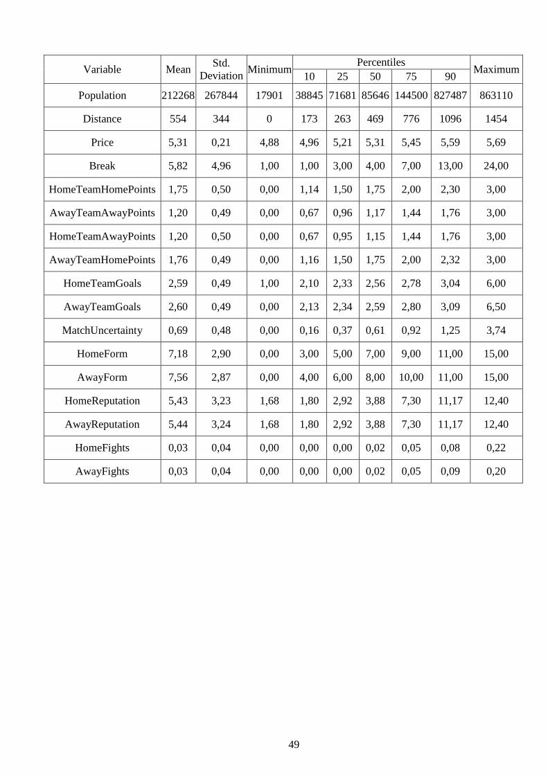
49
Variable Mean Std.
Deviation Minimum
Percentiles Maximum
10 25 50 75 90
Population 212268 267844 17901 38845 71681 85646 144500 827487 863110
Distance 554 344 0 173 263 469 776 1096 1454
Price 5,31 0,21 4,88 4,96 5,21 5,31 5,45 5,59 5,69
Break 5,82 4,96 1,00 1,00 3,00 4,00 7,00 13,00 24,00
HomeTeamHomePoints 1,75 0,50 0,00 1,14 1,50 1,75 2,00 2,30 3,00
AwayTeamAwayPoints 1,20 0,49 0,00 0,67 0,96 1,17 1,44 1,76 3,00
HomeTeamAwayPoints 1,20 0,50 0,00 0,67 0,95 1,15 1,44 1,76 3,00
AwayTeamHomePoints 1,76 0,49 0,00 1,16 1,50 1,75 2,00 2,32 3,00
HomeTeamGoals 2,59 0,49 1,00 2,10 2,33 2,56 2,78 3,04 6,00
AwayTeamGoals 2,60 0,49 0,00 2,13 2,34 2,59 2,80 3,09 6,50
MatchUncertainty 0,69 0,48 0,00 0,16 0,37 0,61 0,92 1,25 3,74
HomeForm 7,18 2,90 0,00 3,00 5,00 7,00 9,00 11,00 15,00
AwayForm 7,56 2,87 0,00 4,00 6,00 8,00 10,00 11,00 15,00
HomeReputation 5,43 3,23 1,68 1,80 2,92 3,88 7,30 11,17 12,40
AwayReputation 5,44 3,24 1,68 1,80 2,92 3,88 7,30 11,17 12,40
HomeFights 0,03 0,04 0,00 0,00 0,00 0,02 0,05 0,08 0,22
AwayFights 0,03 0,04 0,00 0,00 0,00 0,02 0,05 0,09 0,20
Related Documents