FACIAL EXPRESSION RECOGNITION AND TRACKING BASED ON DISTRIBUTED LOCALLY LINEAR EMBEDDING AND EXPRESSION MOTION ENERGY YANG YONG (B.Eng., Xian Jiaotong University ) A THESIS SUBMITTED FOR THE DEGREE OF MASTER OF ENGINEERING DEPARTMENT OF ELECTRICAL AND COMPUTER ENGINEERING NATIONAL UNIVERSITY OF SINGAPORE 2006

Welcome message from author
This document is posted to help you gain knowledge. Please leave a comment to let me know what you think about it! Share it to your friends and learn new things together.
Transcript

FACIAL EXPRESSION RECOGNITION AND
TRACKING BASED ON DISTRIBUTED
LOCALLY LINEAR EMBEDDING AND
EXPRESSION MOTION ENERGY
YANG YONG
(B.Eng., Xian Jiaotong University )
A THESIS SUBMITTED
FOR THE DEGREE OF MASTER OF ENGINEERING
DEPARTMENT OF ELECTRICAL AND COMPUTER
ENGINEERING
NATIONAL UNIVERSITY OF SINGAPORE
2006

Acknowledgements
First and foremost, I would like to take this opportunity to express my sincere
gratitude to my supervisors, Professor Shuzhi Sam Ge and Professor Lee Tong
Heng, for their inspiration, encouragement, patient guidance and invaluable advice,
especially for their selflessly sharing their invaluable experiences and philosophies,
through the process of completing the whole project.
I would also like to extend my appreciation to Dr Chen Xiangdong, Dr Guan
Feng, Dr Wang Zhuping, Mr Lai Xuecheng, Mr Fua Chengheng, Mr Yang Chen-
guang, Mr Han Xiaoyan and Mr Wang Liwang for their help and support.
I am very grateful to National University of Singapore for offering the research
scholarship.
Finally, I would like to give my special thanks to my parents, Yang Guangping
and Dong Shaoqin, my girl friend Chen Yang and all members of my family for
their continuing support and encouragement during the past two years.
ii

Acknowledgements iii
Yang Yong
September 2006

Contents
Acknowledgements ii
Summary viii
List of Tables x
List of Figures xi
1 Introduction 1
1.1 Facial Expression Recognition Methods . . . . . . . . . . . . . . . . 3
1.1.1 Face Detection Techniques . . . . . . . . . . . . . . . . . . . 3
1.1.2 Facial Feature Points Extraction . . . . . . . . . . . . . . . . 7
1.1.3 Facial Expression Classification . . . . . . . . . . . . . . . . 10
1.2 Motivation of Thesis . . . . . . . . . . . . . . . . . . . . . . . . . . 15
1.3 Thesis Structure . . . . . . . . . . . . . . . . . . . . . . . . . . . . . 19
1.3.1 Framework . . . . . . . . . . . . . . . . . . . . . . . . . . . 19
iv

Contents v
1.3.2 Thesis Organization . . . . . . . . . . . . . . . . . . . . . . 20
2 Face Detection and Feature Extraction 23
2.1 Projection Relations . . . . . . . . . . . . . . . . . . . . . . . . . . 24
2.2 Face Detection and Location using Skin Information . . . . . . . . . 26
2.2.1 Color Model . . . . . . . . . . . . . . . . . . . . . . . . . . . 26
2.2.2 Gaussian Mixed Model . . . . . . . . . . . . . . . . . . . . . 28
2.2.3 Threshold & Compute the Similarity . . . . . . . . . . . . . 30
2.2.4 Histogram Projection Method . . . . . . . . . . . . . . . . . 30
2.2.5 Skin & Hair Method . . . . . . . . . . . . . . . . . . . . . . 33
2.3 Facial Features Extraction . . . . . . . . . . . . . . . . . . . . . . . 34
2.3.1 Eyebrow Detection . . . . . . . . . . . . . . . . . . . . . . . 35
2.3.2 Eyes Detection . . . . . . . . . . . . . . . . . . . . . . . . . 36
2.3.3 Nose Detection . . . . . . . . . . . . . . . . . . . . . . . . . 37
2.3.4 Mouth Detection . . . . . . . . . . . . . . . . . . . . . . . . 38
2.3.5 Feature Extraction Results . . . . . . . . . . . . . . . . . . . 38
2.3.6 Illusion & Occlusion . . . . . . . . . . . . . . . . . . . . . . 39
2.4 Facial Features Representation . . . . . . . . . . . . . . . . . . . . . 40
2.4.1 MPEG-4 Face Model Specification . . . . . . . . . . . . . . 42
2.4.2 Facial Movement Pattern for Different Emotions . . . . . . . 48
3 Nonlinear Dimension Reduction (NDR) Methods 54
3.1 Image Vector Space . . . . . . . . . . . . . . . . . . . . . . . . . . . 55
3.2 LLE and NLE . . . . . . . . . . . . . . . . . . . . . . . . . . . . . . 57
3.3 Distributed Locally Linear Embedding (DLLE) . . . . . . . . . . . 60
3.3.1 Estimation of Distribution Density Function . . . . . . . . . 60
Contents vi
3.3.2 Compute the Neighbors of Each Data Point . . . . . . . . . 60
3.3.3 Calculate the Reconstruction Weights . . . . . . . . . . . . . 63
3.3.4 Computative Embedding of Coordinates . . . . . . . . . . . 65
3.4 LLE, NLE and DLLE comparison . . . . . . . . . . . . . . . . . . . 68
4 Facial Expression Energy 71
4.1 Physical Model of Facial Muscle . . . . . . . . . . . . . . . . . . . . 72
4.2 Emotion Dynamics . . . . . . . . . . . . . . . . . . . . . . . . . . . 73
4.3 Potential Energy . . . . . . . . . . . . . . . . . . . . . . . . . . . . 76
4.4 Kinetic Energy . . . . . . . . . . . . . . . . . . . . . . . . . . . . . 80
5 Facial Expression Recognition 83
5.1 Person Dependent Recognition . . . . . . . . . . . . . . . . . . . . . 84
5.1.1 Support Vector Machine . . . . . . . . . . . . . . . . . . . . 88
5.2 Person Independent Recognition . . . . . . . . . . . . . . . . . . . . 93
5.2.1 System Framework . . . . . . . . . . . . . . . . . . . . . . . 94
5.2.2 Optical Flow Tracker . . . . . . . . . . . . . . . . . . . . . . 94
5.2.3 Recognition Results . . . . . . . . . . . . . . . . . . . . . . . 98
6 3D Facial Expression Animation 101
6.1 3D Morphable Models–Xface . . . . . . . . . . . . . . . . . . . . . . 102
6.1.1 3D Avatar Model . . . . . . . . . . . . . . . . . . . . . . . . 103
6.1.2 Definition of Influence Zone and Deformation Function . . . 103
6.2 3D Facial Expression Animation . . . . . . . . . . . . . . . . . . . . 104
6.2.1 Facial Motion Clone Method . . . . . . . . . . . . . . . . . . 104
7 System and Experiments 106

Contents vii
7.1 System Description . . . . . . . . . . . . . . . . . . . . . . . . . . . 107
7.2 Person Dependent Recognition Results . . . . . . . . . . . . . . . . 110
7.2.1 Embedding Discovery . . . . . . . . . . . . . . . . . . . . . . 110
7.2.2 SVM classification . . . . . . . . . . . . . . . . . . . . . . . 113
7.3 Person Independent Recognition Results . . . . . . . . . . . . . . . 116
8 Conclusion 120
8.1 Summary . . . . . . . . . . . . . . . . . . . . . . . . . . . . . . . . 120
8.2 Future Research . . . . . . . . . . . . . . . . . . . . . . . . . . . . . 121
Bibliography 123

Summary
Facial expression plays an important role in our daily activities. It can provide
sensitive and meaningful cues about emotional response and plays a major role in
human interaction and nonverbal communication. Facial expression analysis and
recognition presents a significant challenge to the pattern analysis and human-
machine interface research community. This research aims to develop an auto-
mated and interactive computer vision system for human facial expression recogni-
tion and tracking based on the facial structure features and movement information.
Our system utilizes a subset of Feature Points (FPs) for describing the facial ex-
pressions which is supported by the MPEG-4 standard. An unsupervised learning
algorithm, Distributed Locally Linear Embedding (DLLE), is introduced to recover
the inherent properties of scattered data lying on a manifold embedded in high-
dimensional input facial images. The selected person-dependent facial expression
images in a video are classified using DLLE. We also incorporate facial expres-
sion motion energy to describe the facial muscle’s tension during the expressions
for person-independent tracking. It takes advantage of the optical flow method
which tracks the feature points’ movement information. By further considering
viii

Summary ix
different expressions’ temporal transition characteristics, we are able to pin-point
the actual occurrence of specific expressions with higher accuracy. A 3D realistic
interactive head model is created to derive multiple virtual expression animations
according to the recognition results. A virtual robotic talking head for human
emotion understanding and intelligent human computer interface is realized.

List of Tables
2.1 Facial animation parameter units and their definitions . . . . . . . . 45
2.2 Quantitative FAPs modeling . . . . . . . . . . . . . . . . . . . . . . 46
2.3 The facial movements cues for six emotions. . . . . . . . . . . . . . 49
2.4 The movements clues of facial features for six emotions . . . . . . . 53
7.1 Conditions under which our system can operate . . . . . . . . . . . 107
7.2 Recognition results using DLLE and SVM(1V1) for training data . 115
7.3 Recognition results using DLLE and SVM(1V1) for testing data . . 115
x

List of Figures
1.1 The basic facial expression recognition framework. . . . . . . . . . 3
1.2 The horizontal and vertical signature. . . . . . . . . . . . . . . . . . 4
1.3 Six universal facial expressions . . . . . . . . . . . . . . . . . . . . . 11
1.4 Overview of the system framework. . . . . . . . . . . . . . . . . . . 19
2.1 Projection relations between the real world and the virtual world. . 25
2.2 Projection relationship between a real head and 3D model. . . . . . 26
2.3 Fitting skin color into Gaussian distribution. . . . . . . . . . . . . . 29
2.4 Face detection using vertical and horizontal histogram method . . . 31
2.5 Face detection using hair and face skin method. . . . . . . . . . . . 32
2.6 The detected rectangle face boundary. . . . . . . . . . . . . . . . . 33
2.7 Sample experimental face detection results. . . . . . . . . . . . . . . 34
2.8 The rectangular feature-candidate areas of interest. . . . . . . . . . 35
2.9 The outline model of the left eye. . . . . . . . . . . . . . . . . . . . 37
2.10 The outline model of the mouth. . . . . . . . . . . . . . . . . . . . . 38
xi

List of Figures xii
2.11 Feature label . . . . . . . . . . . . . . . . . . . . . . . . . . . . . . 39
2.12 Sample experimental facial feature extraction results. . . . . . . . . 40
2.13 The feature extraction results with glasses. . . . . . . . . . . . . . . 41
2.14 Anatomy image of face muscles. . . . . . . . . . . . . . . . . . . . . 42
2.15 The facial feature points . . . . . . . . . . . . . . . . . . . . . . . . 43
2.16 Face model with FAPUs . . . . . . . . . . . . . . . . . . . . . . . . 45
2.17 The facial coordinates. . . . . . . . . . . . . . . . . . . . . . . . . . 50
2.18 Facial muscle movements for six emotions . . . . . . . . . . . . . . 51
3.1 Image illustrated as point vector . . . . . . . . . . . . . . . . . . . . 56
3.2 Information redundancy problem . . . . . . . . . . . . . . . . . . . 59
3.3 The neighbor selection process. . . . . . . . . . . . . . . . . . . . . 62
3.4 Twopeaks . . . . . . . . . . . . . . . . . . . . . . . . . . . . . . . . 68
3.5 Punched sphere . . . . . . . . . . . . . . . . . . . . . . . . . . . . . 69
4.1 The mass spring face model. . . . . . . . . . . . . . . . . . . . . . . 73
4.2 Smile expression motion . . . . . . . . . . . . . . . . . . . . . . . . 74
4.3 The temporal curve of one mouth point in smile expression . . . . . 75
4.4 The potential energy of mouth points. . . . . . . . . . . . . . . . . 78
4.5 3D spatio-temporal potential motion energy mesh . . . . . . . . . . 79
5.1 The first two coordinates of DLLE of some samples. . . . . . . . . . 85
5.2 2D projection using different NDR methods. . . . . . . . . . . . . . 87
5.3 3D projection using different NDR methods. . . . . . . . . . . . . . 88
5.4 Optimal separating hyperplane. . . . . . . . . . . . . . . . . . . . . 91
5.5 The framework of our tracking system. . . . . . . . . . . . . . . . . 93
List of Figures xiii
5.6 Feature tracked using optical flow method . . . . . . . . . . . . . . 99
5.7 Real-time video tracking results. . . . . . . . . . . . . . . . . . . . . 100
6.1 3D head model. . . . . . . . . . . . . . . . . . . . . . . . . . . . . . 102
6.2 Influence zone of feature points . . . . . . . . . . . . . . . . . . . . 104
6.3 The facial motion clone method illustration. . . . . . . . . . . . . . 105
7.1 The interface of the our system. . . . . . . . . . . . . . . . . . . . . 108
7.2 The 3D head model interface for expression animation. . . . . . . . 109
7.3 The first two coordinates using different NDR methods. . . . . . . . 110
7.4 The first three coordinates using different NDR methods. . . . . . . 112
7.5 The SVM classification results for Fig. 7.3(d) . . . . . . . . . . . . 113
7.6 The SVM classification for different sample sets. . . . . . . . . . . . 114
7.7 Real-time video tracking results in different environment. . . . . . . 118
7.8 Real-time video tracking results for other testers. . . . . . . . . . . 119

Chapter 1Introduction
Facial expression plays an important role in our daily activities. The human face
is a rich and powerful source full of communicative information about human be-
havior and emotion. The most expressive way that humans display emotions is
through facial expressions. Facial expression includes a lot of information about
human emotion. It is one of the most important carriers of human emotion, and
it is a significant way for understanding human emotion. It can provide sensitive
and meaningful cues about emotional response and plays a major role in human
interaction and nonverbal communication. Humans can detect faces and interpret
facial expressions in a scene with little or no effort.
The origins of facial expression analysis go back into the 19th century, when Dar-
win proposed the concept of universal facial expressions in human and animals. In
his book, “The Expression of the Emotions in Man and Animals” [1], he noted:
“...the young and the old of widely different races, both with man and animals,
express the same state of mind by the same movements.”
1

2
In recent years there has been a growing interest in developing more intelligent
interface between humans and computers, and improving all aspects of the in-
teraction. This emerging field has attracted the attention of many researchers
from several different scholastic tracks, i.e., computer science, engineering, psy-
chology, and neuroscience. These studies focus not only on improving computer
interfaces, but also on improving the actions the computer takes based on feed-
back from the user. There is a growing demand for multi-modal/media human
computer interface (HCI). The main characteristics of human communication are:
multiplicity and multi-modality of communication channels. A channel is a com-
munication medium while a modality is a sense used to perceive signals from the
outside world. Examples of human communication channels are: auditory channel
that carries speech, auditory channel that carries vocal intonation, visual channel
that carries facial expressions, and visual channel that carries body movements.
Recent advances in image analysis and pattern recognition open up the possibil-
ity of automatic detection and classification of emotional and conversational facial
signals. Automating facial expression analysis could bring facial expressions into
man-machine interaction as a new modality and make the interaction tighter and
more efficient. Facial expression analysis and recognition are essential for intelli-
gent and natural HCI, which presents a significant challenge to the pattern analysis
and human-machine interface research community. To realize natural and harmo-
nious HCI, computer must have the capability for understanding human emotion
and intention effectively. Facial expression recognition is a problem which must
be overcome for future prospective application such as: emotional interaction,
interactive video, synthetic face animation, intelligent home robotics, 3D games
and entertainment. An automatic facial expression analysis system mainly include
three important parts: face detection, facial feature points extraction and facial
expression classification.
1.1 Facial Expression Recognition Methods 3
1.1 Facial Expression Recognition Methods
The development of an automated system which can detect faces and interpret
facial expressions is rather difficult. There are several related problems that need
to be solved: detection of an image segment as a face, extraction of the facial
expression information, and classification of the expression into different emotion
categories. A system that performs these operations accurately and in real-time
would be a major step forward in achieving a human-like interaction between the
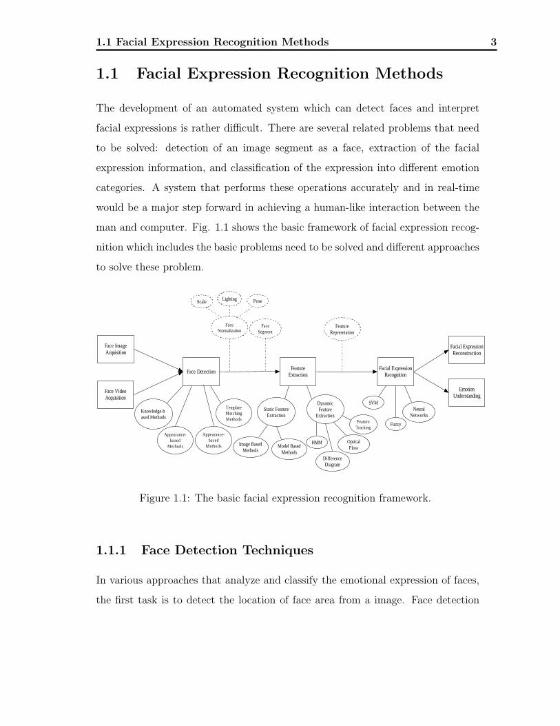
man and computer. Fig. 1.1 shows the basic framework of facial expression recog-
nition which includes the basic problems need to be solved and different approaches
to solve these problem.
Face ImageAcquisition
Knowledge-based Methods
Appearance-based
Methods
TemplateMatchingMethods
Static FeatureExtraction
DynamicFeature
Extraction
Facial ExpressionRecognition
Facial ExpressionReconstruction
FeatureExtractionFace Detection
DifferenceDiagram
HMM OpticalFlow
EmotionUnderstanding
Face VideoAcquisition
Appearance-based
Methods Image BasedMethods
Model BasedMethods
FeatureTracking
FaceNormalization
SVMNeural
Networks
Fuzzy
Scale Lighting Pose
FaceSegment
FeatureRepresetation
Figure 1.1: The basic facial expression recognition framework.
1.1.1 Face Detection Techniques
In various approaches that analyze and classify the emotional expression of faces,
the first task is to detect the location of face area from a image. Face detection
1.1 Facial Expression Recognition Methods 4
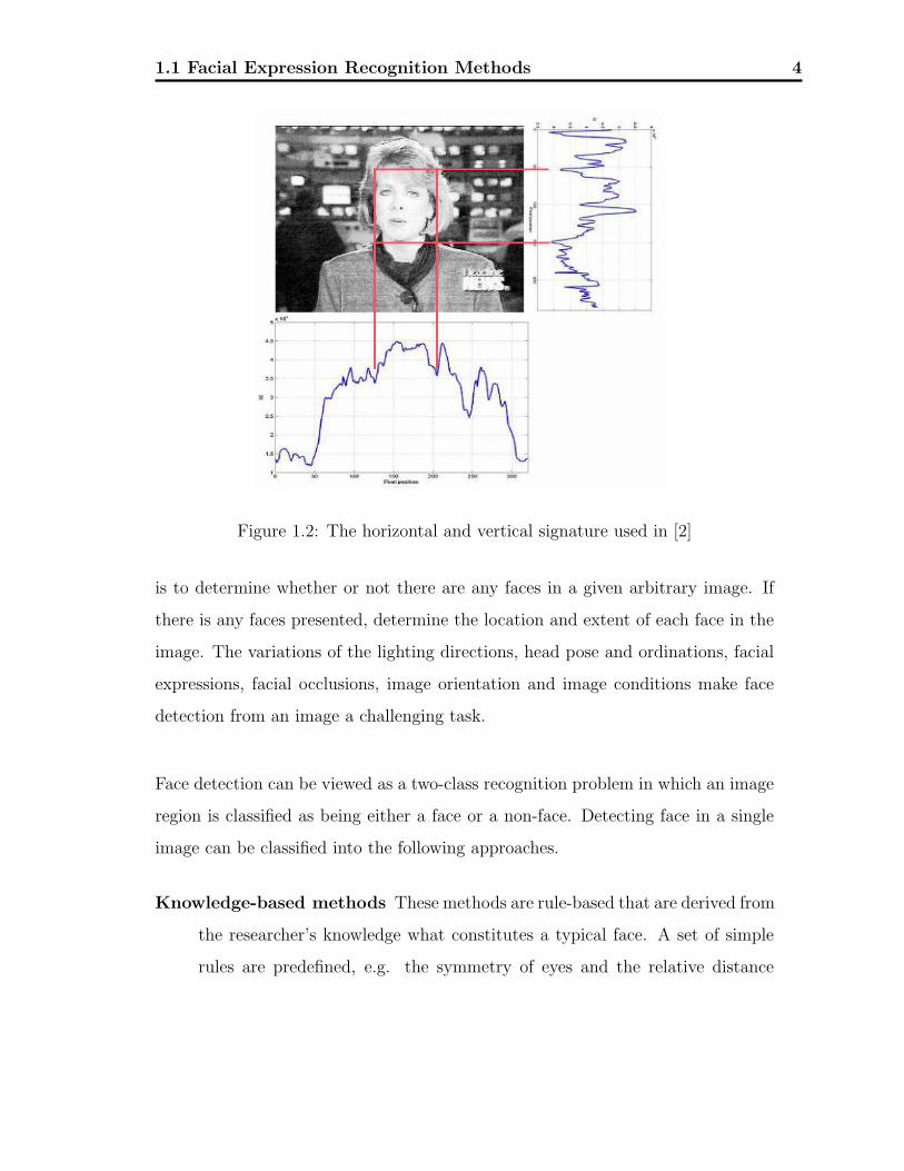
Figure 1.2: The horizontal and vertical signature used in [2]
is to determine whether or not there are any faces in a given arbitrary image. If
there is any faces presented, determine the location and extent of each face in the
image. The variations of the lighting directions, head pose and ordinations, facial
expressions, facial occlusions, image orientation and image conditions make face
detection from an image a challenging task.
Face detection can be viewed as a two-class recognition problem in which an image
region is classified as being either a face or a non-face. Detecting face in a single
image can be classified into the following approaches.
Knowledge-based methods These methods are rule-based that are derived from
the researcher’s knowledge what constitutes a typical face. A set of simple
rules are predefined, e.g. the symmetry of eyes and the relative distance

1.1 Facial Expression Recognition Methods 5
between nose and eyes. The facial features are extracted and the face can-
didates are identified subsequently based on the predefined rules. In 1994,
Yang and Huang presented a rule-based location method with a hierarchical
structure consisting of three levels [3]. Kotropoulos and Pitas [2] presented
a rule-based localization procedure which is similar to [3]. The facial bound-
ary are located using the horizontal and vertical projections [4]. Fig. 1.2
shows an example where the boundaries of the face correspond to the local
minimum of the histogram.
Feature invariant methods These approaches attempt to find out the facial
structure features that are invariant to pose, viewpoint or lighting condi-
tions. The human skin color has been widely used as an important cue and
proven to be an effective feature for face area detection. The specific facial
features include eyebrows, eyes, nose and mouth can be extracted using edge
detectors. Sirohey presented a facial localization method which makes use of
the edge map and generates an ellipse contour to fit the boundary of face [5].
Graf et al. proposed a method to locate the faces and facial features using
gray scale images [6]. The histogram peaks and width are utilized to per-
form adoptive image segmentation by computing an adoptive threshold. The
threshold is used to generate binarized images and connected area that are
identified to locate the candidate facial features. These areas are combined
and evaluated with classifier later to determine where the face is located.
Sobottka and Pitas presented a method to locate skin-like region using shape
and color information to perform color segmentation in the HSV color space
[7]. By using the region growth method, the connected components are de-
termined. For each connected components, the best-fit ellipse is computed
and if it fits well, it is selected as a face candidate.
1.1 Facial Expression Recognition Methods 6
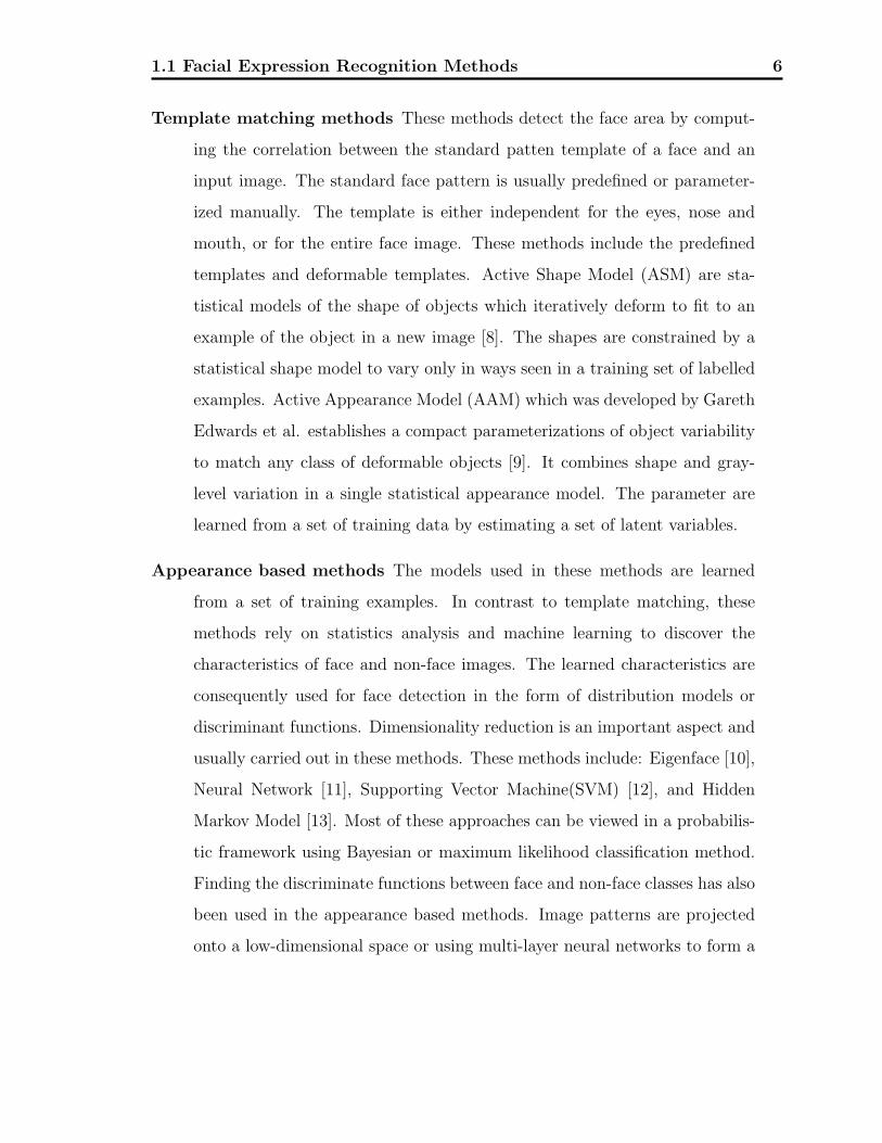
Template matching methods These methods detect the face area by comput-
ing the correlation between the standard patten template of a face and an
input image. The standard face pattern is usually predefined or parameter-
ized manually. The template is either independent for the eyes, nose and
mouth, or for the entire face image. These methods include the predefined
templates and deformable templates. Active Shape Model (ASM) are sta-
tistical models of the shape of objects which iteratively deform to fit to an
example of the object in a new image [8]. The shapes are constrained by a
statistical shape model to vary only in ways seen in a training set of labelled
examples. Active Appearance Model (AAM) which was developed by Gareth
Edwards et al. establishes a compact parameterizations of object variability
to match any class of deformable objects [9]. It combines shape and gray-
level variation in a single statistical appearance model. The parameter are
learned from a set of training data by estimating a set of latent variables.
Appearance based methods The models used in these methods are learned
from a set of training examples. In contrast to template matching, these
methods rely on statistics analysis and machine learning to discover the
characteristics of face and non-face images. The learned characteristics are
consequently used for face detection in the form of distribution models or
discriminant functions. Dimensionality reduction is an important aspect and
usually carried out in these methods. These methods include: Eigenface [10],
Neural Network [11], Supporting Vector Machine(SVM) [12], and Hidden
Markov Model [13]. Most of these approaches can be viewed in a probabilis-
tic framework using Bayesian or maximum likelihood classification method.
Finding the discriminate functions between face and non-face classes has also
been used in the appearance based methods. Image patterns are projected
onto a low-dimensional space or using multi-layer neural networks to form a

1.1 Facial Expression Recognition Methods 7
nonlinear decision surface.
Face detection is the preparatory step for the following work. For example, it can fix
a range of interests, decrease the searching range and initial approximation area for
the feature selection. In our system, we assume and only consider the situation that
there is only one face contained in one image. The face takes up a significant area
in the image. Although the detection of multiple faces in one image is realizable,
due to the image resolution, head pose variation, occlusion and other problems, it
will greatly increase the difficulty of detecting facial expression if there are multiple
faces in one image. The facial features will be more prominent if one face takes up
a large area of image. The face location for expression recognition mainly deal with
two problems: the head pose variation and the illumination variation since they
can greatly affect the following feature extraction. Generally, facial image needs
to be normalized first to remove the effect of head pose and illumination variation.
The ideal head pose is that the facial plane is parallel to the project image. The
obtained image from such pose has the least facial distortion. The illumination
variation can greatly affect the brightness of the image and make it more difficult
to extract features. Using a fixed lighting can avoid the illumination problem, but
affect the robustness of the algorithm. The most common method to remove the
illumination variation is using Gabor Filter on the input images [14]. Besides, there
are some other work for removing the ununiformity of facial brightness caused by
illumination and variation of reflection coefficient of different facial parts [15].
1.1.2 Facial Feature Points Extraction
The goal of facial feature points detection is to obtain the facial feature’s variety
and the face’s movements. Under the assumption that there is only one face in
an image, feature points extraction includes detecting the presence and locating of
features, such as eyes, nose, nostrils, eyebrow, mouth, lips, ears, etc [16]. The face

1.1 Facial Expression Recognition Methods 8
feature detection method can be classified according to whether the operation is
based on global movements or local movements. It could also be classified accord-
ing to whether the extraction is based on the facial features’s transformation or
the whole face muscle’s movement. Until now, there is no uniform solution. Each
method has its advantages and is operated under certain conditions.
The facial features can be treated as permanent and temporary. The permanent
ones are unremovable features existing on face. They will transform wrt. the face
muscle’s movement, e.g. the eyes, eyebrow, mouth and so on. The temporary
features mainly include the temporary wrinkles. They will appear with the move-
ment of the face and disappear when the movement is over. They are not constant
features on the face.
The method based on global deformation is to extract all the permanent and tem-
porary information. Most of the time, it is required to do background substraction
to remove the effect of the background. The method based on local deformation
is to decompose the face into several sub areas and find the local feature informa-
tion. Feature extraction is done in each individual sub areas independently. The
local features can be represented using Principal Components Analysis(PCA) and
described using the intensity profiles or gradient analysis.
The method based on the image feature extraction does not depend on the priority
knowledge. It extracts the features only based on the image information. It is fast
and simple, but lack robustness and reliability. The method need to model the face
features first according to priority knowledge. It is more complex and time con-
suming, but more reliable. This feature extraction method can be further divided
according to the dimension of the model. The method is based on 2D information
1.1 Facial Expression Recognition Methods 9
to extract the features without considering the depth of the object. The method is
based on 3D information considering the geometry information of the face. There
are two typical 3D face models: face muscle model [17] and face movement model
[18]. 3D face model is more complicated and time consuming compared to 2D face
model. It is the muscle’s movements that result in the appearance change of face,
and the change of appearance is the reflection of muscle’s movement.
Face movement detection method attempted to extract the displacement relative
information from two adjacent temporal frames. These information is obtained
by comparing the current facial expression and the neutral face. The neutral face
is necessary for extracting the alteration information, but not always needed in
the feature movement detection method. Most of the reference face used in this
method is the previous frame. The classical optical flow method is to use the
correlation of two adjacent frames for estimation [19]. The movement detection
method can be only used in the video sequence while the deformation extraction
can be adopted in either a single image or a video sequence. But the deforma-
tion extraction method could not get the detailed information such as each pixel’s
displacement information while the method based on facial movement can extract
these information much easier.
Face deformation includes two aspects: the changes of face shape and texture. The
change of texture will cause the change of gradient of the image. Most of the meth-
ods based on the shape distortion extract these gradient change caused by different
facial expressions. High pass filter and Gabor filter [20] can be adopted to detect
such gradient information. It has been proved that the Gabor filter is a powerful
method used in image feature extraction. The texture could be easily affected by
the illumination. The Gabor filter can remove the illumination variation effects

1.1 Facial Expression Recognition Methods 10
[21]. Active Appearance Model(AAM) were developed by Gareth Edwards et al.
[9] which establishes a compact parameterizations of object variability to match
any of a class of deformable objects. It combines shape and gray-level variation
in a single statistical appearance model. The parameters learned are from a set of
training data by estimating a set of latent variables.
In 1995, Essa et al. proposed two methods using dynamic model and motion en-
ergy to classify facial expressions [22]. One is based on the physical model where
expression is classified by comparison of estimated muscle activations. The other
is to use the spacial-temporal motion energy templates of the whole face for each
facial expression. The motion energy is converted from the muscles activations.
Both methods show substantially great recognition accuracy. However, the author
did not give a clear definition of the motion energy. At the same time, they only
used the spatial information in their recognition pattern. By considering differ-
ent expressions’ temporal transition characteristics, a higher recognition accuracy
could be achieved.
1.1.3 Facial Expression Classification
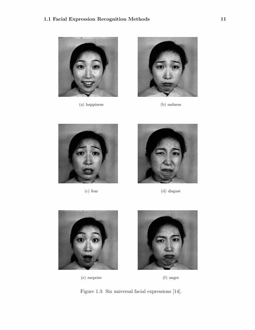
According to the psychological and neurophysiological studies, there are six basic
emotions-happiness, sadness, fear, disgust, surprise, and anger as shown in Fig.
1.3. Each basic emotion is associated with one unique facial expression.
Since 1970s, Ekman and Friesen have performed extensive studies on human facial
expressions and developed an anatomically oriented coding system for describing
all visually distinguishable facial movements, called the facial action coding sys-
tem (FACS) [23]. It is used for analyzing and synthesizing facial expression based
1.1 Facial Expression Recognition Methods 11
(a) happiness (b) sadness
(c) fear (d) disgust
(e) surprise (f) anger
Figure 1.3: Six universal facial expressions [14].
1.1 Facial Expression Recognition Methods 12
on 46 Action Units (AU) which describe basic facial movements. Each AU may
correspond to several muscles’ activities which are composed to a certain facial
expression. FACS are used manually to describe the facial expressions, using still
images when the facial expression is at its apex state. The FACS model has re-
cently inspired interests to analyze facial expressions by tracking facial features
or measuring the amount of facial movement. Its derivation of facial animation
and definition parameters has been adopted in the framework of the ISO MPEG-4
standard. The MPEG-4 standardization effort grew out of the wish to create a
video-coding standard more capable than previous versions [24].
Facial expression classification mainly deal with the task of categorizing active and
spontaneous facial expressions to extract information of the underlying human
emotional states. Based on the face detection and feature extraction results, the
analysis of the emotional expression can be carried out. A large number of meth-
ods have been developed for facial expression analysis. These approaches could be
divided into two main categories: target oriented and gesture oriented. The target
oriented approaches [25, 26, 27] attempt to infer the human emotion and classify
the facial expression from one single image containing one typical facial expression.
The gesture oriented methods [28, 29] make use of the temporal information from a
sequence of facial expression motion images. In particular, transitional approaches
attempt to compute the facial expressions from the facial neural condition and
expressions at the apex. Fully dynamic techniques extract facial emotions through
a sequence of images.
The target oriented approaches can be subdivided into template matching meth-
ods and rule based methods. Tian et al. developed an anatomic face analysis
system based on both permanent and transient facial features [30]. Multistate

1.1 Facial Expression Recognition Methods 13
facial component models such as lips and eyes are proposed for tracking. Tem-
plate matching and neural networks are used in the system to recognize 16 AUs
in nearly frontal-view face image sequences. Pantic et al. developed an automatic
system to recognize facial gestures in static, frontal and profile view face images
[31]. By making use of the action unions (AUs), a rule-based method is adopted
which achieves 86 % recognition rate.
Facial expression is a dynamic process. How to fully make use of the dynamic infor-
mation can be critical to the recognition result. There is a growing argument that
the temporal information is a critical factor in the interpretation of facial expres-
sions [32]. Essa et al. examined the temporal pattern of different expressions but
did not account for temporal aspects of facial motion in their recognition feature
vector [33]. Roivainen et al. developed a system using a 3D face mesh based on the
FACS model [34]. The motion of the head and facial expressions is estimated in
model-based facial image coding. An algorithm for recovering rigid and nonrigid
motion of the face was derived based on two, or more frames. The facial images
are analyzed for the purpose of re-synthesizing a 3D head model. Donato et al.
used independent component analysis (IDA), optical flow estimation and Gabor
wavelet representation methods that achieved 95.5% average recognition rate as
reported in [35].
In transitional approaches, its focus is on computing motion of either facial muscles
or facial features between neutral and apex instances of a face. Mase described two
approaches–top-down and bottom-up–based on facial muscle’s motion [36]. In the
top-down method, the facial image is divided into muscle units that correspond
to the AUs defined in FACS. Optical flow is computed within rectangles that in-
clude these muscle units, which in turn can be related to facial expressions. This

1.1 Facial Expression Recognition Methods 14
approach relies heavily on locating rectangles containing the appropriate muscles,
which is a difficult image analysis problem. In the bottom-up method, the area
of the face is tessellated with rectangular regions over which optical flow feature
vectors are computed; a 15-dimensional feature space is considered, based on the
mean and variance of the optical flow. Recognition of expressions is then based on
k-nearest-neighbor voting rule.
The fully dynamic approaches make use of temporal and spatial information. The
methods using both temporal and spatial are called spatial-time methods while the
methods only using the spatial information are called spatial methods.
Optical flow approach is widely adopted using the dense motion fields computed
frame by frame. It falls into two classes: global optical flow and local optical flow
methods. The global method can extract information of the whole facial region’s
movements. However, it is computationally intensive and sensitive to the contin-
uum of the movements. The local optical flow method can improve the speed by
only computing the motion fields in selected regions and directions. The Lucas-
Kanade optical flow algorithm [37], is capable of following and recovering the facial
points lost due to lighting variations, rigid or non-rigid motion, or (to a certain
extent) change of head orientation. It can achieve high efficiency and tracking
accuracy.
In feature tracing approach, it could not track each pixel’s movement like optical
flow; motions are estimated only over a selected set of prominent features in the
face image. Each image in the video sequence is first processed to detect the promi-
nent facial features, such as edges, eyes, brows and mouth. The analysis of the
image motion is carried out subsequently, in particular, tracked by Lucas-Kanade

1.2 Motivation of Thesis 15
algorithm. Yacoob used the local parameters to model the mouth, nose, eyebrows
and eyelids and used dense sequences to capture expressions over time [28]. It was
based on qualitative tracking of principal regions of the face and flow computation
at high intensity gradient points.
Neural networks is a typical spatial method. It takes the whole raw image, or
processed image such as: Gabor filtered, or eigen-image: such as PCA and ICA,
as the input of the network. Most of the time, it is not easy to train the neural
network for a good result.
Hidden markov models (HMM) is also used to extract facial feature vectors for its
ability to deal with time sequences and to provide time scale invariance, as well
as its learning capabilities. Ohya et al. assigned the condition of facial muscles to
a hidden state of the model for each expression and used the wavelet transform
to extract features from facial images [29]. A sequence of feature vectors were
obtained in different frequency bands of the image, by averaging the power of
these bands in the areas corresponding to the eyes and the mouth. Some other
work also employ HMM to design classifier which can recognize different facial
expressions successfully [38, 39].
1.2 Motivation of Thesis
The objective of our research is to develop an automated and interactive computer
vision system for human facial expression recognition and tracking based on the
facial structure features and movement information. Recent advances in the image
processing and pattern analysis open up the possibility of automatic detection and
classification of emotional and conversational facial signals. Most of the previous

1.2 Motivation of Thesis 16
work on the spatio-temporal analysis for facial expression understanding, however,
suffer the following shortcomings:
• The facial motion information is obtained mostly by computing holistic dense
flow between successive image frames. However, dense flow computing is
quite time-consuming.
• Most of these technologies can not respond in real-time to the facial expres-
sions of a user. The facial motion pattern has to be trained offline, whereas
the trained model limits its reliability for realistic applications since facial ex-
pressions involve great interpersonal variations and a great number of possible
facial AU combinations. For spontaneous behavior, the facial expressions are
particularly difficult to be segmented by a neutral state in an observed image
sequence.
• The approaches do not consider the intensity scale of the different facial
expressions. Each individual has his/her own maximal intensity of displaying
a particular facial action. A better description about the facial muscles’s
tension is needed.
• Facial expression is a dynamic processes. Most of the current technics adopt
the facial texture information as the vectors for further recognition [8], or
combined with the facial shape information [9]. There are more information
stored in the facial expression sequence compared to the facial shape informa-
tion. Its temporal information can be divided into three discrete expression
states in an expression sequence: the beginning, the peak, and the ending of
the expression. However, the existing approaches do not measure the facial
movement itself and are not able to model the temporal evolution and the
momentary intensity of an observed facial expression, which are indeed more
informative in human behavior analysis.

1.2 Motivation of Thesis 17
• There is usually a huge amount of information in the captured images, which
makes it difficult to analyze the human facial expressions. The raw data,
facial expression images, can be viewed as that they define a manifold in
the high-dimensional image space, which can be further used for facial ex-
pression analysis. Therefore, dimension reduction is critical for analyzing the
images, to compress the information and to discover compact representations
of variability.
• A facial expression consists of not only its temporal information, but also a
great number of AU combinations and transient cues. The HMM can model
uncertainties and time series, but it lacks the ability to represent induced
and nontransitive dependencies. Other methods, e.g., NNs, lack the suffi-
cient expressive power to capture the dependencies, uncertainties, and tem-
poral behaviors exhibited by facial expressions. Spatio-temporal approaches
allow for facial expression dynamics modeling by considering facial features
extracted from each frame of a facial expression video sequence.
Compared with other existing approaches on facial expression recognition, the
proposed method enjoys several favorable properties which overcome these short-
comings:
• Do not need to compute the holistic dense flow but rather after the key facial
features are captured, optical flow are computed just for these features.
• One focus of our work is to address problems with previous solutions of their
slowness and requirement for some degree of manual intervention. Auto-
matically face detection and facial feature extraction are realized. Real-time
processing for person-independent recognition are implemented in our sys-
tem.

1.2 Motivation of Thesis 18
• Facial expression motion energy are defined to describe the individual’s facial
muscle’s tension during the expressions for person independent tracking. It
is proposed by analyzing different facial expression’s unique spacial-temporal
pattern.
• To compress the information and to discover compact representations, we
proposed a new Distributed Locally Linear Embedding (DLLE) to discover
the inherent properties of the input data.
Besides, there are several other characters in our system.
• Only one web camera is utilized
• Rigid head motions allowed.
• Variations in lighting conditions allowed
• Variation of background allowed
Our facial expression recognition research is conducted based on the following
assumptions:
Assumption 1. Using only vision camera, one can only detect and recognize the
shown emotion that may or may not be the personal true emotions. It is assumed
that the subject shows emotions through facial expressions as a mean to express
emotion.
Assumption 2. Theories of psychology claim that there is a small set of basic ex-
pressions [23], even if it is not universally accepted. A recent cross-cultural study
confirms that some emotions have a universal facial expression across the cultures
and the set proposed by Ekman [40] is a very good choice. Six basic emotions-
happiness, sadness, fear, disgust, surprise, and anger are considered in our re-
search. Each basic emotion is assumed associated with one unique facial expression
for each person.
1.3 Thesis Structure 19
Assumption 3. There is only one face contained in the captured image. The face
takes up a significant area in the image. The image resolution should be sufficiently
large to facilitate feature extraction and tracking .
1.3 Thesis Structure
1.3.1 Framework
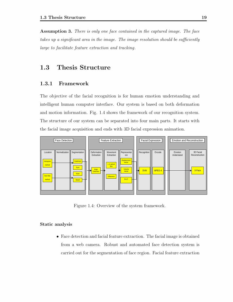
The objective of the facial recognition is for human emotion understanding and
intelligent human computer interface. Our system is based on both deformation
and motion information. Fig. 1.4 shows the framework of our recognition system.
The structure of our system can be separated into four main parts. It starts with
the facial image acquisition and ends with 3D facial expression animation.
Face Detection
Location Normalization Segmentation
Feature Extraction
DeformationExtraction
MovementExtraction
Representation
Facial Expression
Recognition Encode
Emotion and Reconstruction
EmotionUnderstand
3D FacialReconstruction
Histogram
method
Hair-Skin
method
Eyebrows
Eyes
Nose
Mouth
L-K opticalflow
Difference
EdgeDetection X-FaceMPEG-4SVM
DisplacementVector
VelocityVector
DLLE
Figure 1.4: Overview of the system framework.
Static analysis
• Face detection and facial feature extraction. The facial image is obtained
from a web camera. Robust and automated face detection system is
carried out for the segmentation of face region. Facial feature extraction
1.3 Thesis Structure 20
include locating the position and shape of the eyebrows, eyes, nose,
mouth, and extracting features related to them in a still image of human
face. Image analysis techniques are utilized which can automatically
extract meaningful information from facial expression motion without
manual operation to construct feature vectors for recognition.
• Dimensionality reduction. In this stage, the dimension of the motion
curve is reduced by analyzing with our proposed Distributed Locally
Linear Embedding (DLLE). The goal of dimensionality reduction is to
obtain a more compact representation of the original data, a represen-
tation that preservers all the information for further decision making.
• Perform classification using SVM. Once the facial data are transformed
into a low-dimensional space, SVM is employed to classify the input
facial pattern image into various emotion category.
Dynamic analysis
• The process is carried out using one web camera in real-time. It utilize
the dynamics of features to identify expressions.
• Facial expression motion energy. It is used to describe the facial muscle’s
tension during the expressions for person-independent tracking.
3D virtual facial animation
• A 3D facial model is created based on MPEG-4 standard to derive mul-
tiple virtual character expressions in response to the user’s expression.
1.3.2 Thesis Organization
The remainder of this thesis is organized as follows:
1.3 Thesis Structure 21
In Chapter 2, face detection and facial features extraction methods are discussed.
Face detection can fix a range of interests, decrease the searching range and initial
approximation area for the feature selection. Two methods, using vertical and
horizontal projections and skin-hair information, are conducted to automatically
detect and locate face area. A subset of Feature Points (FPs) is utilized in our
system for describing the facial expressions which is supported by the MPEG-4
standard. Facial feature are extracted using deformable templates to get precise
positions.
In Chapter 3, an unsupervised learning algorithm, distributed locally linear embed-
ding (DLLE), is introduced which can recover the inherent properties of scattered
data lying on a manifold embedded in high-dimensional input facial images. The in-
put high-dimensional facial expression images are embeded into a low-dimensional
space while the intrinsic structures are maintained and main characteristics of the
facial expression are kept.
In Chapter 4, we propose facial expression motion energy to describe the facial
muscle’s tension during the expressions for person independent tracking. The fa-
cial expression motion energy is composed of potential energy and kinetic energy.
It takes advantage of the optical flow method which tracks the feature points’
movement information. For each expression we use the typical patterns of muscle
actuation, as determined by a detailed physical analysis, to generate the typical
pattern of motion energy associated with each facial expression. By further con-
sidering different expressions’ temporal transition characteristics, we are able to
pinpoint the actual occurrence of specific expressions with higher accuracy.
In Chapter 5, both static person dependent and dynamic person independent facial

1.3 Thesis Structure 22
expression recognition methods are discussed. For the person dependent recogni-
tion, we utilize the similarity of facial expressions appearance in low-dimensional
embedding to classify different emotions. This method is based on the observa-
tion that facial expression images define a manifold in the high-dimensional image
space, which can be further used for facial expression analysis. For the person
independent facial expression classification, facial expression energy can be used
by adjusting the general expression pattern to a particular individual according to
the individual’s successful expression recognition results.
In Chapter 6, a 3D virtual interactive expression model is created and applied
into our face recognition and tracking system to derive multiple realistic character
expressions. The 3D avatar model is parameterized according to the MPEG-4 fa-
cial animation standard. Realistic 3D virtual expressions are animated which can
follow the object’s facial expression.
In Chapters 7 and 8, we present the experimental results with our system and the
conclusion of this thesis respectively.
Chapter 2Face Detection and Feature Extraction
Human face detection has been researched extensively over the past decade, due to
the recent emergence of applications such as security access control, visual surveil-
lance, content-based information retrieval, and advanced human-to-computer in-
teraction. It is also the first task performed in a face recognition system. To
ensure good results in the subsequent recognition phase, face detection is a cru-
cial procedure. In the last ten years, face and facial expression recognition have
attracted much attention, though they truly have been studied for more than 20
years by psychophysicists, neuroscientists and engineers. Many research demon-
strations and commercial applications have been developed from these efforts. The
first step of any face processing system is to locate all faces that are present in a
given image. However, face detection from a single image is a challenging task be-
cause of the high degree of spatial variability in scale, location and pose (rotated,
frontal, profile). Facial expression, occlusion and lighting conditions also change
the overall appearance of faces, as described in reference [41].
To build fully-automated systems that analyze the information contained in face
23
2.1 Projection Relations 24
images, robust and efficient face detection algorithms are required. Such a prob-
lem is challenging, because faces are non-rigid objects that have a high degree of
variability in size, shape, color and texture. Therefore, to obtain robust automated
systems, one must be able to detect faces within images in an efficient and highly
reproducible manner. In reference [41], the author gave a definition of face detec-
tion: “Given an arbitrary image, the goal of face detection is to determine whether
or not there are any faces in the image and, if present, return the image location
and extent of each face”.
In this chapter, face detection and facial features extraction methods are discussed.
Two methods of face detection, using vertical and horizontal histogram projections
approach and skin-hair information approach, are discussed which can automat-
ically detect face area. Face detection initializes the approximation area for the
following feature selection. Facial feature are extracted using deformable templates
to get precise positions. A subset of Feature Points (FPs), which is supported by
the MPEG-4 standard, is described which are used in later section for expression
modeling.
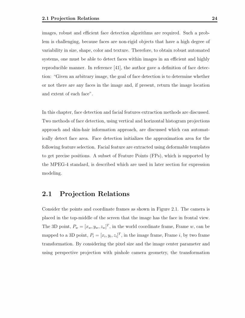
2.1 Projection Relations
Consider the points and coordinate frames as shown in Figure 2.1. The camera is
placed in the top-middle of the screen that the image has the face in frontal view.
The 3D point, Pw = [xw, yw, zw]T , in the world coordinate frame, Frame w, can be
mapped to a 3D point, Pi = [xi, yi, zi]T , in the image frame, Frame i, by two frame
transformation. By considering the pixel size and the image center parameter and
using perspective projection with pinhole camera geometry, the transformation
2.1 Projection Relations 25
from Pw to point Ps = [xs, ys, 0]T in the screen frame, Frame s, is given by [42]:
xs =f
sx
xw
zw
+ ox
ys =f
sy
yw
zw
+ oy (2.1)
where sx, sy are the width and length of a pixel on the screen, ox, oy is the origin
of Frame s, and the f is the focal length.
Y
Z
X
w
w
w
Ow
Y
ZX
i
ii
Oi
Pw
P i
L1
L2
Screen Space
Y
Z
X
s
s
s
Os
Web Camera
Figure 2.1: Projection relations between the real world and the virtual world.
The corresponding image point Pi can be expressed by a rigid body transformation:
Pi = RisPs + P i
sorg (2.2)
where Ris ∈ R
3×3 is the rotational matrix, P isorg ∈ R
3 is the origin of Frame s with
respect to Frame i.
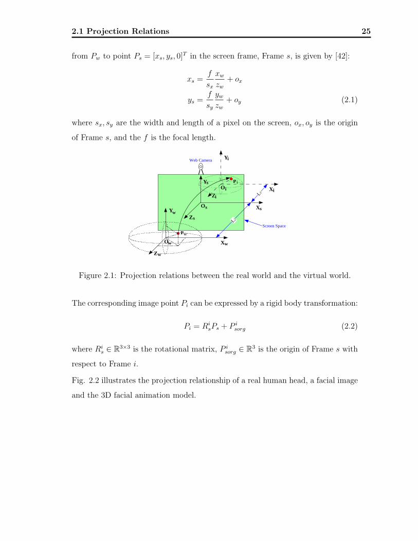
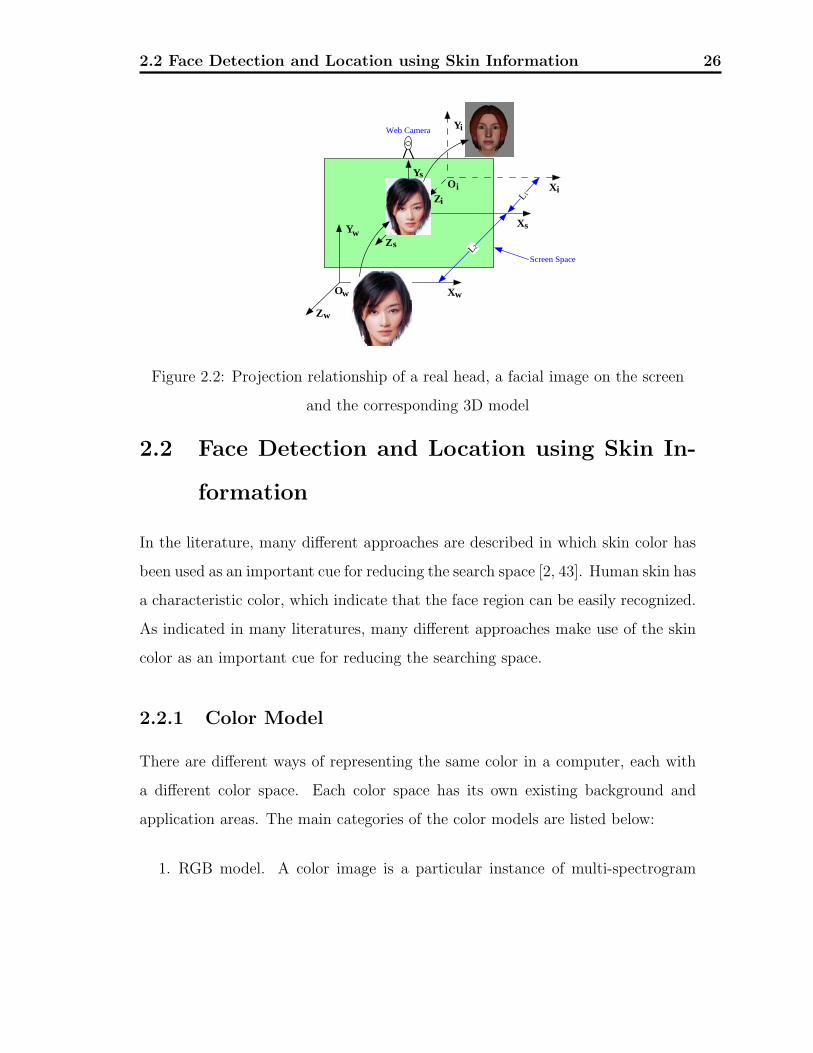
Fig. 2.2 illustrates the projection relationship of a real human head, a facial image
and the 3D facial animation model.
2.2 Face Detection and Location using Skin Information 26
Y
Z
X
w
w
w
O
Y
ZX
i
ii
Oi
L1
L2
Screen Space
Y
Z
X
s
s
s
Os
Web Camera
w
Figure 2.2: Projection relationship of a real head, a facial image on the screen
and the corresponding 3D model
2.2 Face Detection and Location using Skin In-
formation
In the literature, many different approaches are described in which skin color has
been used as an important cue for reducing the search space [2, 43]. Human skin has
a characteristic color, which indicate that the face region can be easily recognized.
As indicated in many literatures, many different approaches make use of the skin
color as an important cue for reducing the searching space.
2.2.1 Color Model
There are different ways of representing the same color in a computer, each with
a different color space. Each color space has its own existing background and
application areas. The main categories of the color models are listed below:
1. RGB model. A color image is a particular instance of multi-spectrogram
2.2 Face Detection and Location using Skin Information 27
which corresponds to the three frequency band of the three visional base
colors (i.e. Red, Green and Blue). It is popular to use RGB components as
the format to represent colors. Most image acquisition equipment is based
on CCD technology which perceives the RGB component of colors. Yet the
method of RGB representation is very sensitive to perimeter light, making it
difficult to segregate human skin from the background.
2. HSI(hue, saturation, intensity) model. This format reflects the way that peo-
ple observe colors and is beneficial to image handling. The advantage of this
format is its capability of segregating the two parameters that reflect the
characteristics of colors C Hue and Saturation. When we are extracting the
color characteristics of some object (e.g. face), we need to know its clustering
characteristics in certain color space. Generally, the clustering characteris-
tics are represented in the intrinsic characteristics of colors, and are often
affected by illumination. The intensity component is directly influenced by
illumination. So if we can extract an intensity component out from colors,
and only use the hue and saturation that reflect the intrinsic characteristics
of colors to carry out clustering analysis, we can achieve a better effect. This
is the reason that a HSI format is frequently used in color image processing
and computer vision.
3. YCbCr model. YCbCr model is widely applied in areas such as TV dis-
play and is also the representation format applied in many video frequency
compression codes such as MPEG, JPEG standards. It has the following
advantages: 1. Like HSI model, it can segregate the brightness component,
but the calculation process and representation of space coordinates are rel-
atively simple. 2. It has similar uses to the perception process of human
vision. YCbCr can be achieved by RGB through linear transformation, the
ITU.BT-601 transformation formula is as below.
2.2 Face Detection and Location using Skin Information 28
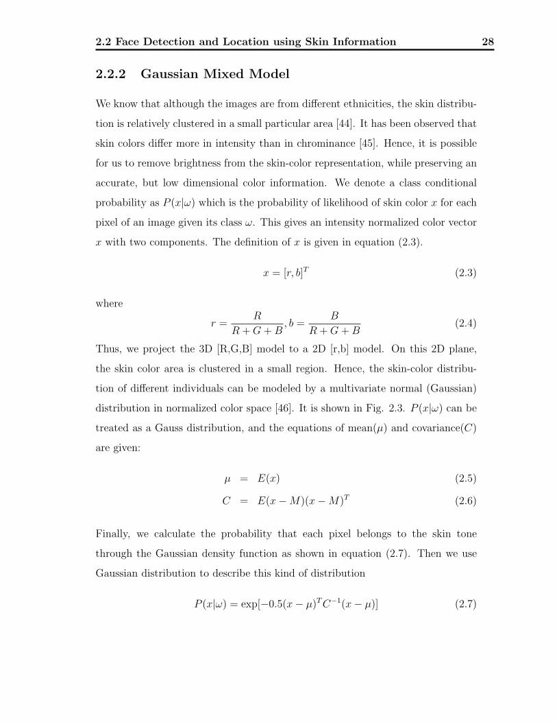
2.2.2 Gaussian Mixed Model
We know that although the images are from different ethnicities, the skin distribu-
tion is relatively clustered in a small particular area [44]. It has been observed that
skin colors differ more in intensity than in chrominance [45]. Hence, it is possible
for us to remove brightness from the skin-color representation, while preserving an
accurate, but low dimensional color information. We denote a class conditional
probability as P (x|ω) which is the probability of likelihood of skin color x for each
pixel of an image given its class ω. This gives an intensity normalized color vector
x with two components. The definition of x is given in equation (2.3).
x = [r, b]T (2.3)
where
r =R
R + G + B, b =
B
R + G + B(2.4)
Thus, we project the 3D [R,G,B] model to a 2D [r,b] model. On this 2D plane,
the skin color area is clustered in a small region. Hence, the skin-color distribu-
tion of different individuals can be modeled by a multivariate normal (Gaussian)
distribution in normalized color space [46]. It is shown in Fig. 2.3. P (x|ω) can be
treated as a Gauss distribution, and the equations of mean(μ) and covariance(C)
are given:
μ = E(x) (2.5)
C = E(x−M)(x−M)T (2.6)
Finally, we calculate the probability that each pixel belongs to the skin tone
through the Gaussian density function as shown in equation (2.7). Then we use
Gaussian distribution to describe this kind of distribution
P (x|ω) = exp[−0.5(x− μ)T C−1(x− μ)] (2.7)
2.2 Face Detection and Location using Skin Information 29
Figure 2.3: Fitting skin color into Gaussian distribution.
Through the distance between two pixels and the center we can get the information
on how similar it is to skin and get a distribution histogram similar to the original
image. The probability should be between 0 and 1, because we normalize the three
components (R, G, B) of each pixel’s color at the beginning. The probability of
each pixel is multiplied by 255 in order to create a gray-level image I(x, y). This
image is also called a likelihood image. The computed likelihood image is shown
in Fig. 2.4(c).
2.2 Face Detection and Location using Skin Information 30
2.2.3 Threshold & Compute the Similarity
After obtaining the likelihood of skin I(x, y), a binary image B(x, y) can be ob-
tained by thresholding each pixel’s I(x, y) with a threshold T according to
B(x, y) =
⎧⎪⎨⎪⎩
0, if I(x, y) > T
1, if I(x, y) ≤ T
(2.8)
There is no definite criterion to determine a threshold. If the threshold value is too
big, the false rate will increase. On the other hand, if the threshold is too small,
the missed rate will increase. This detection threshold can be adjusted to trade-off
between correct detections and false positives. According to the previous research
work [47], we adopt the threshold value as 0.5. That is, when the skin probability
of a certain pixel is larger or equal to 0.5, we will regard the pixel as skin. In Fig.
2.4(b), the binary image B(x, y) is derived from the I(x, y) according to the rule
defined in equation (2.8). As observed from the experiments, if the background
color is similar to skin, there will be more candidate regions, and the follow-up
verifying time will increase.
2.2.4 Histogram Projection Method
We have used integral projections of the histogram map of the face image for facial
area location [47]. The vertical and horizontal projection vectors in the image
rectangle [x1, x2]× [y1, y2] are defined as:
V (x) =
y=y2∑y=y1
B(x, y) (2.9)
H(x) =
x=x2∑x=x1
B(x, y) (2.10)
The face area is located by applying sequentially the analysis of the vertical his-
togram and then the horizontal histogram. The peaks of the vertical histogram of

2.2 Face Detection and Location using Skin Information 31
(a) The vertical histogram (b) The binary image
(c) The likelihood image (d) The horizontal histogram
Figure 2.4: Face detection using vertical and horizontal histogram method
the head box correspond with the border between the hair and the forehead, the
eyes, the nostrils, the mouth and the boundary between the chin and the neck.
The horizontal line going through the eyes goes through the local maximum of the
second peak. The x axis of the vertical line going between the eyes and through the
nose is chosen as the absolute minimum of the contrast differences found along the
horizontal line going through the eyes. By performing the analysis of the vertical
and the horizontal histogram, the eyes’ area is reduced so that it contains just the
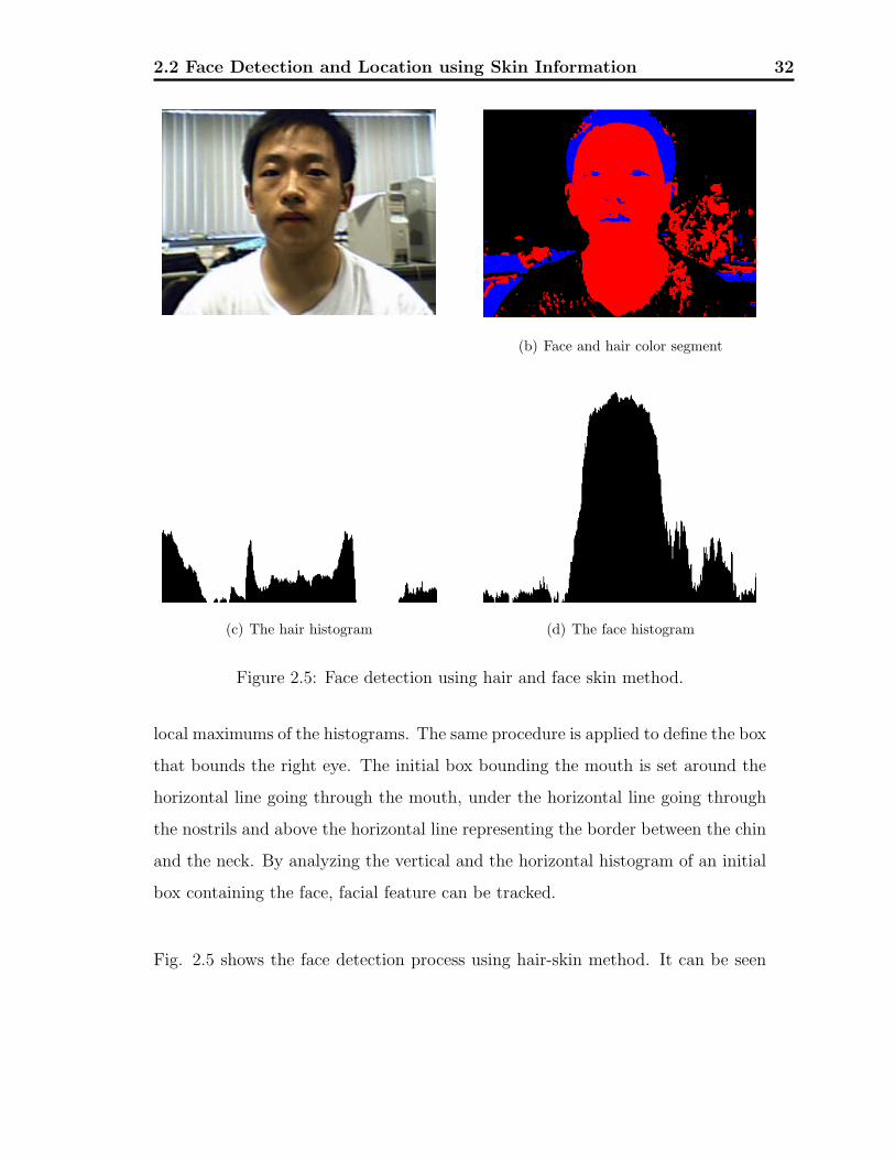
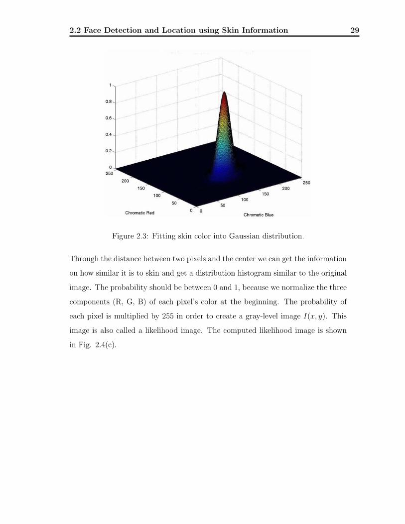
2.2 Face Detection and Location using Skin Information 32
(a) The original face image (b) Face and hair color segment
(c) The hair histogram (d) The face histogram
Figure 2.5: Face detection using hair and face skin method.
local maximums of the histograms. The same procedure is applied to define the box
that bounds the right eye. The initial box bounding the mouth is set around the
horizontal line going through the mouth, under the horizontal line going through
the nostrils and above the horizontal line representing the border between the chin
and the neck. By analyzing the vertical and the horizontal histogram of an initial
box containing the face, facial feature can be tracked.
Fig. 2.5 shows the face detection process using hair-skin method. It can be seen
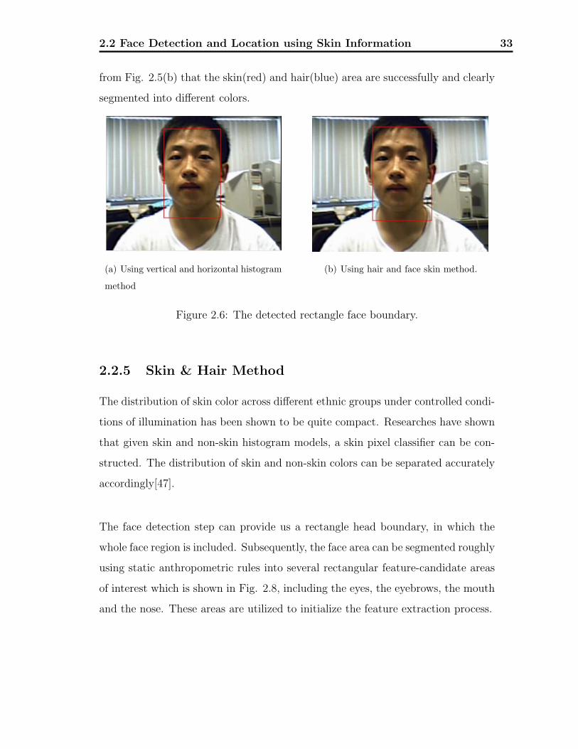
2.2 Face Detection and Location using Skin Information 33
from Fig. 2.5(b) that the skin(red) and hair(blue) area are successfully and clearly
segmented into different colors.
(a) Using vertical and horizontal histogram
method
(b) Using hair and face skin method.
Figure 2.6: The detected rectangle face boundary.
2.2.5 Skin & Hair Method
The distribution of skin color across different ethnic groups under controlled condi-
tions of illumination has been shown to be quite compact. Researches have shown
that given skin and non-skin histogram models, a skin pixel classifier can be con-
structed. The distribution of skin and non-skin colors can be separated accurately
accordingly[47].
The face detection step can provide us a rectangle head boundary, in which the
whole face region is included. Subsequently, the face area can be segmented roughly
using static anthropometric rules into several rectangular feature-candidate areas
of interest which is shown in Fig. 2.8, including the eyes, the eyebrows, the mouth
and the nose. These areas are utilized to initialize the feature extraction process.
2.3 Facial Features Extraction 34
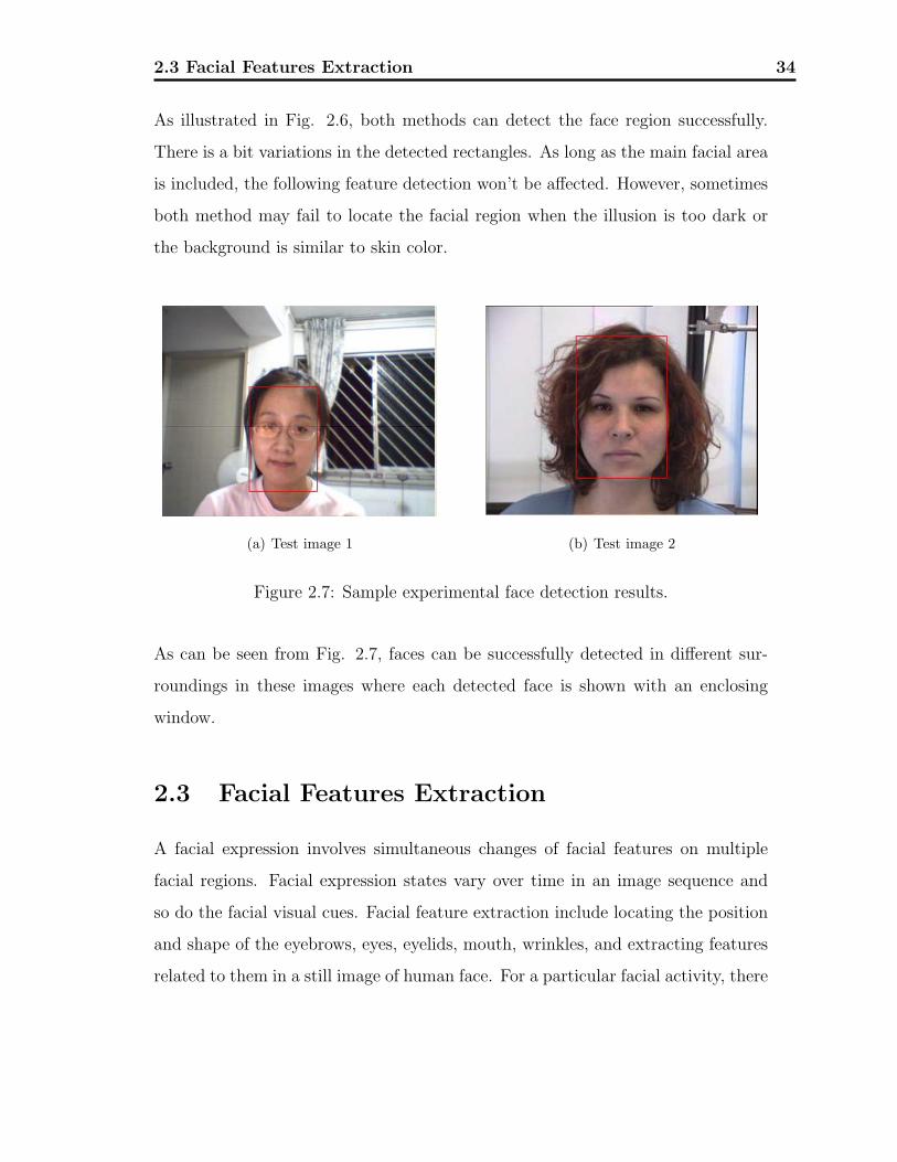
As illustrated in Fig. 2.6, both methods can detect the face region successfully.
There is a bit variations in the detected rectangles. As long as the main facial area
is included, the following feature detection won’t be affected. However, sometimes
both method may fail to locate the facial region when the illusion is too dark or
the background is similar to skin color.
(a) Test image 1 (b) Test image 2
Figure 2.7: Sample experimental face detection results.
As can be seen from Fig. 2.7, faces can be successfully detected in different sur-
roundings in these images where each detected face is shown with an enclosing
window.
2.3 Facial Features Extraction
A facial expression involves simultaneous changes of facial features on multiple
facial regions. Facial expression states vary over time in an image sequence and
so do the facial visual cues. Facial feature extraction include locating the position
and shape of the eyebrows, eyes, eyelids, mouth, wrinkles, and extracting features
related to them in a still image of human face. For a particular facial activity, there

2.3 Facial Features Extraction 35
is a subset of facial features that are the most informative and maximally reduces
the ambiguity of classification. Therefore we actively and purposefully select 21
facial visual cues to achieve a desirable result in a timely and efficient manner while
reducing the ambiguity of classification to a minimum. In our system, features are
extracted using deformable templates with details given below.
Figure 2.8: The rectangular feature-candidate areas of interest.
2.3.1 Eyebrow Detection
The segmentation algorithm cannot give bounding box for the eyebrow exclusively.
Brunelli suggests use of template matching for extracting the eye, but we use
another approach as described below. Eyebrow is segmented from eye using the
fact that the eye occurs below eyebrow and its edges form closed contours, obtained
by applying Laplacian of Gaussian operator at zero threshold. These contours are
filled and the resulting image containing masks of eyebrow and eye. From the two
2.3 Facial Features Extraction 36
largest filled regions, the region with higher centroid is chosen to be the mask of
eyebrow.
2.3.2 Eyes Detection
The positions of eyes are determined by searching for minima in the topographic
grey level relief. The contour of the eyes can be precisely found. Since the real
images are always affected by the lighting and noises, it is not robust and often
require expert supervision using the general local detection method such as corner
detection [48]. The Snake algorithm is much more robust, but rely much on the
image itself and there may be too many details in the result [49]. We can make
full use of the priority knowledge of human face which describes the eyes as piece-
wise polynomial. A more precise contour can be obtained by making use of the
deformable template.
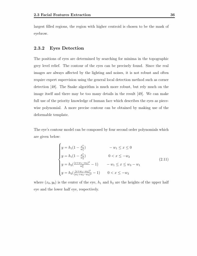
The eye’s contour model can be composed by four second order polynomials which
are given below:
⎧⎪⎪⎪⎪⎪⎪⎪⎪⎨⎪⎪⎪⎪⎪⎪⎪⎪⎩
y = h1(1− x2
w21) − w1 ≤ x ≤ 0
y = h1(1− x2
w22) 0 < x ≤ −w2
y = h2((x+w1−w3)2
w23
− 1) − w1 ≤ x ≤ w3 − w1
y = h2((x+w1−w3)2
(w1+w2−w3)2− 1) 0 < x ≤ −w2
(2.11)
where (x0, y0) is the center of the eye, h1 and h2 are the heights of the upper half
eye and the lower half eye, respectively.
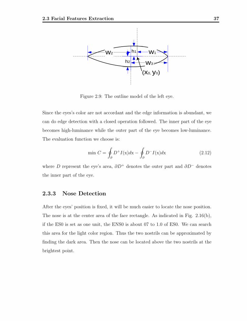
2.3 Facial Features Extraction 37
h1
h2
w1
w3
w2
(x0, y0)
Figure 2.9: The outline model of the left eye.
Since the eyes’s color are not accordant and the edge information is abundant, we
can do edge detection with a closed operation followed. The inner part of the eye
becomes high-luminance while the outer part of the eye becomes low-luminance.
The evaluation function we choose is:
min C =
∮∂
D+I(x)dx−∮
∂
D−I(x)dx (2.12)
where D represent the eye’s area, ∂D+ denotes the outer part and ∂D− denotes
the inner part of the eye.
2.3.3 Nose Detection
After the eyes’ position is fixed, it will be much easier to locate the nose position.
The nose is at the center area of the face rectangle. As indicated in Fig. 2.16(b),
if the ES0 is set as one unit, the ENS0 is about 07 to 1.0 of ES0. We can search
this area for the light color region. Thus the two nostrils can be approximated by
finding the dark area. Then the nose can be located above the two nostrils at the
brightest point.
2.3 Facial Features Extraction 38
2.3.4 Mouth Detection
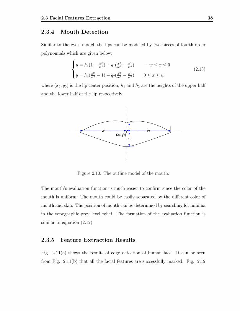
Similar to the eye’s model, the lips can be modeled by two pieces of fourth order
polynomials which are given below:⎧⎪⎨⎪⎩
y = h1(1− x2
w2 ) + q1(x2
w2 − x4
w4 ) − w ≤ x ≤ 0
y = h2(x2
w2 − 1) + q2(x2
w2 − x4
w4 ) 0 ≤ x ≤ w
(2.13)
where (x0, y0) is the lip center position, h1 and h2 are the heights of the upper half
and the lower half of the lip respectively.
(x0, y0)
h1
h2
w w
Figure 2.10: The outline model of the mouth.
The mouth’s evaluation function is much easier to confirm since the color of the
mouth is uniform. The mouth could be easily separated by the different color of
mouth and skin. The position of mouth can be determined by searching for minima
in the topographic grey level relief. The formation of the evaluation function is
similar to equation (2.12).
2.3.5 Feature Extraction Results
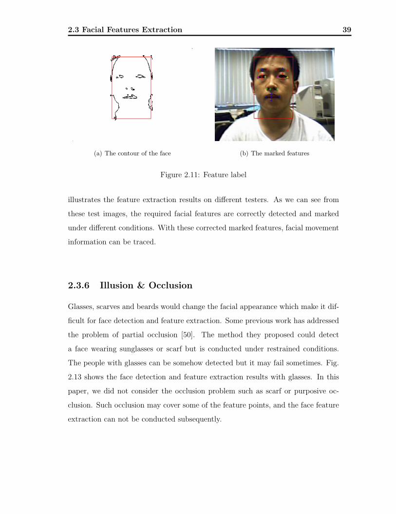
Fig. 2.11(a) shows the results of edge detection of human face. It can be seen
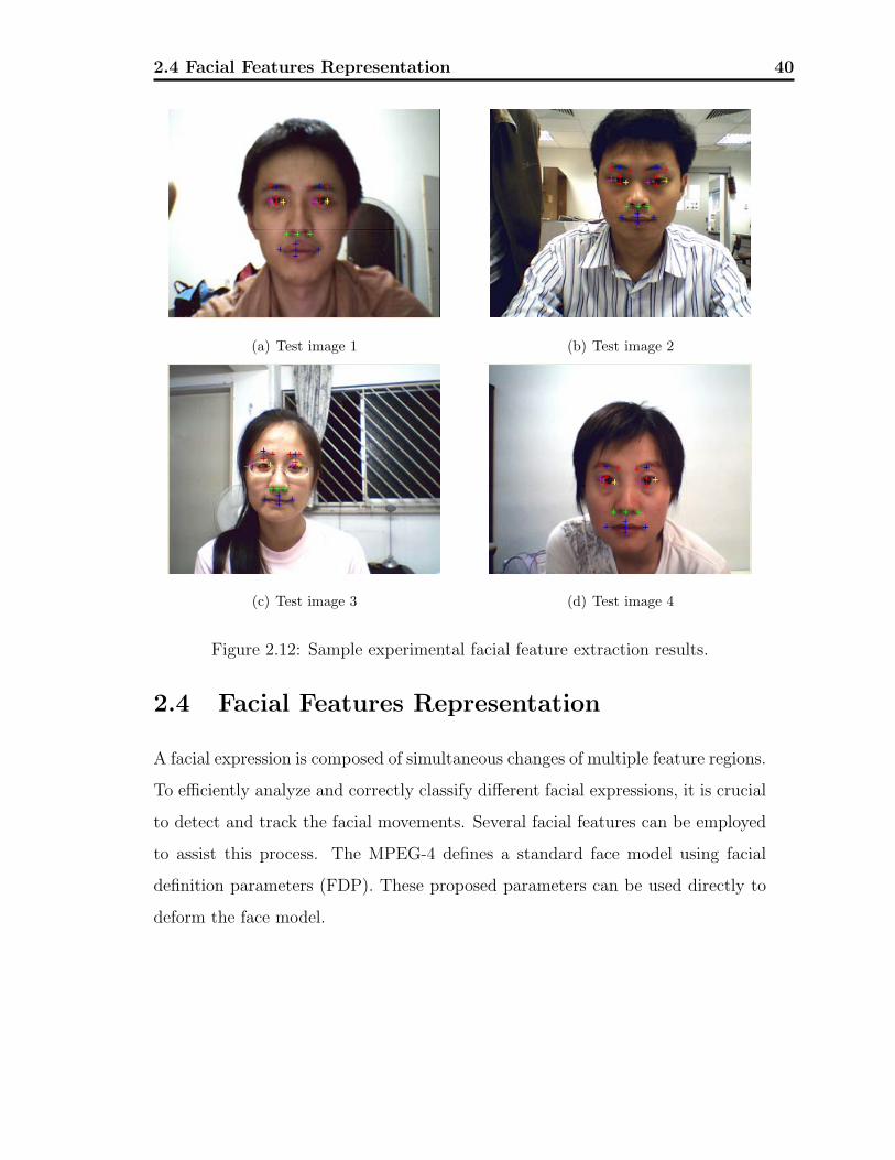
from Fig. 2.11(b) that all the facial features are successfully marked. Fig. 2.12
2.3 Facial Features Extraction 39
(a) The contour of the face (b) The marked features
Figure 2.11: Feature label
illustrates the feature extraction results on different testers. As we can see from
these test images, the required facial features are correctly detected and marked
under different conditions. With these corrected marked features, facial movement
information can be traced.
2.3.6 Illusion & Occlusion
Glasses, scarves and beards would change the facial appearance which make it dif-
ficult for face detection and feature extraction. Some previous work has addressed
the problem of partial occlusion [50]. The method they proposed could detect
a face wearing sunglasses or scarf but is conducted under restrained conditions.
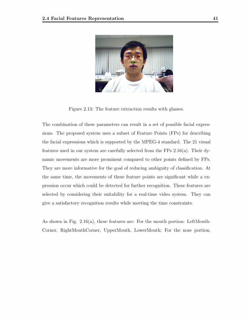
The people with glasses can be somehow detected but it may fail sometimes. Fig.
2.13 shows the face detection and feature extraction results with glasses. In this
paper, we did not consider the occlusion problem such as scarf or purposive oc-
clusion. Such occlusion may cover some of the feature points, and the face feature
extraction can not be conducted subsequently.
2.4 Facial Features Representation 40
(a) Test image 1 (b) Test image 2
(c) Test image 3 (d) Test image 4
Figure 2.12: Sample experimental facial feature extraction results.
2.4 Facial Features Representation
A facial expression is composed of simultaneous changes of multiple feature regions.
To efficiently analyze and correctly classify different facial expressions, it is crucial
to detect and track the facial movements. Several facial features can be employed
to assist this process. The MPEG-4 defines a standard face model using facial
definition parameters (FDP). These proposed parameters can be used directly to
deform the face model.
2.4 Facial Features Representation 41
Figure 2.13: The feature extraction results with glasses.
The combination of these parameters can result in a set of possible facial expres-
sions. The proposed system uses a subset of Feature Points (FPs) for describing
the facial expressions which is supported by the MPEG-4 standard. The 21 visual
features used in our system are carefully selected from the FPs 2.16(a). Their dy-
namic movements are more prominent compared to other points defined by FPs.
They are more informative for the goal of reducing ambiguity of classification. At
the same time, the movements of these feature points are significant while a ex-
pression occur which could be detected for further recognition. These features are
selected by considering their suitability for a real-time video system. They can
give a satisfactory recognition results while meeting the time constraints.
As shown in Fig. 2.16(a), these features are: For the mouth portion: LeftMouth-
Corner, RightMouthCorner, UpperMouth, LowerMouth; For the nose portion,
2.4 Facial Features Representation 42
LeftNostril, RightNostril, NoseTip; for the eye portion: LeftEyeInnerCorner, Left-
EyeOuterCorner, LeftEyeUpper, LeftEyeLower, RightEyeInnerCorner, RightEye-
OuterCorner, RightEyeUpper, RightEyeLower; for the eyebrow portion: LeftEye-
BrowInner, LeftEyeBrowOuter, LeftEyeBrowMiddle, RightEyeBrowInner, RightEye-
BrowOuter, RightEyeBrowMiddle.
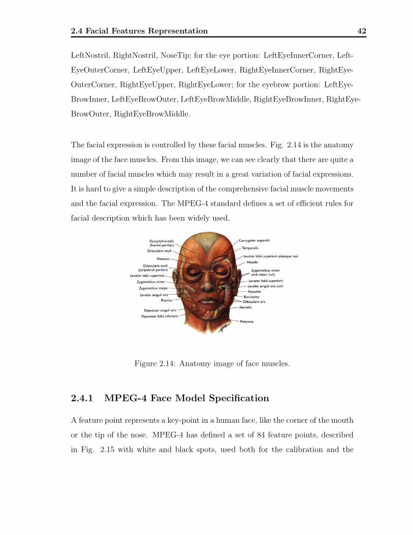
The facial expression is controlled by these facial muscles. Fig. 2.14 is the anatomy
image of the face muscles. From this image, we can see clearly that there are quite a
number of facial muscles which may result in a great variation of facial expressions.
It is hard to give a simple description of the comprehensive facial muscle movements
and the facial expression. The MPEG-4 standard defines a set of efficient rules for
facial description which has been widely used.
Figure 2.14: Anatomy image of face muscles.
2.4.1 MPEG-4 Face Model Specification
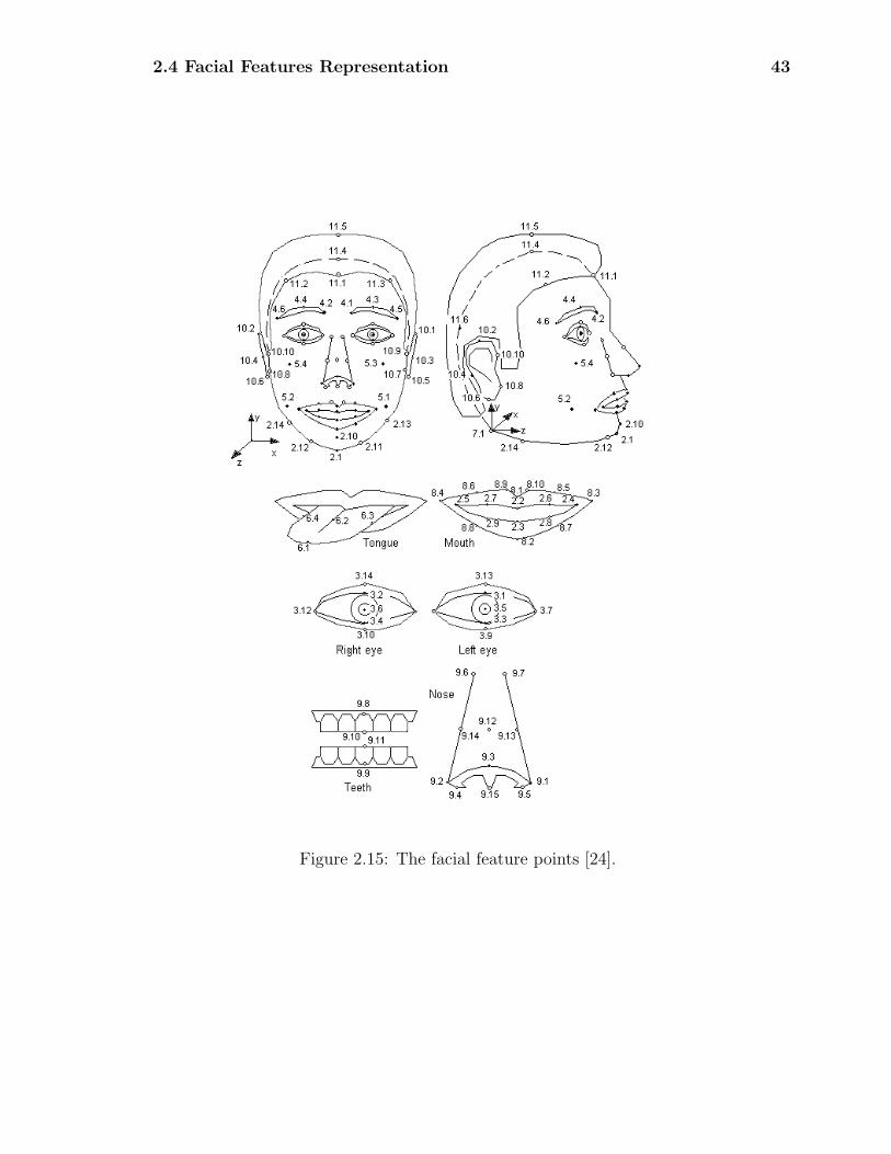
A feature point represents a key-point in a human face, like the corner of the mouth
or the tip of the nose. MPEG-4 has defined a set of 84 feature points, described
in Fig. 2.15 with white and black spots, used both for the calibration and the
2.4 Facial Features Representation 43
Figure 2.15: The facial feature points [24].
2.4 Facial Features Representation 44
animation of a synthetic face. More precisely, all the feature points can be used for
the calibration of a face, while only the black ones are used also for the animation.
Feature points are subdivided in groups according to the region of the face they
belong to, and numbered accordingly.
In order to define FAPs for arbitrary face models, MPEG-4 defines FAPUs that
serve to scale FAPs for any face model. FAPUs are defined as fractions of dis-
tances between key facial features as shown in Fig. 2.16. These features, such
as eye separation are defined on a face model which is in the neutral state. The
FAPU allows interpretation of the FAPs on any facial model in a consistent way
producing reasonable results in terms of expression and speech pronunciation.
Although FAPs provide all the necessary elements for MPEG-4 compatible ani-
mation, they cannot be directly used for the analysis of expressions from video
sequences, due to the absence of a clear quantitative definition. In order to mea-
sure the FAPs in real image sequences, we adopt the mapping between them and
the movement of specific FDP feature points(FPs), which correspond to salient
points on human face. As shown in Fig. 2.16(b), some of these points can be
used as reference points in neutral face. Distances between these points are used
for normalization purposes [51]. The quantitative modeling of FAPs are shown in
Table 2.1 and 2.2.
The MPEG-4 standard defines 68 FAPs. They are divided into ten groups, which
describe the movement of the face. These parameters are either high level param-
eter, that is, parameters that describe visemes and facial expressions, or low-level
parameters which describe displacement of the specific single point of the face.
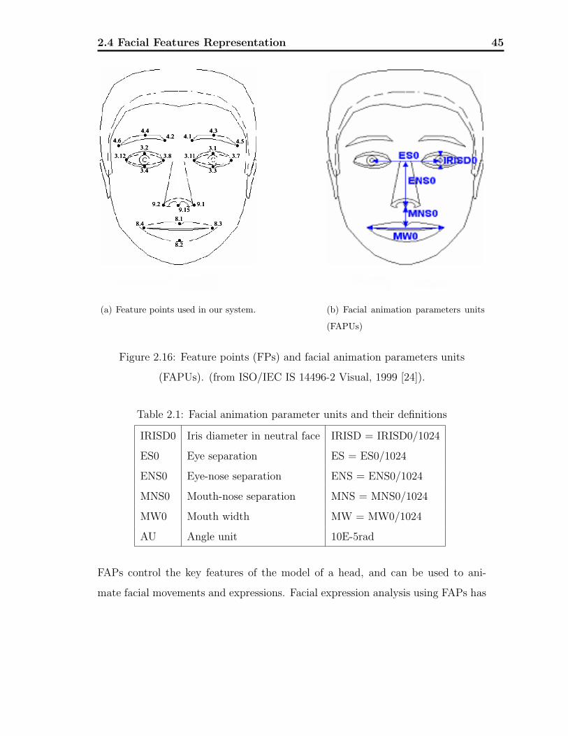
2.4 Facial Features Representation 45
(a) Feature points used in our system. (b) Facial animation parameters units
(FAPUs)
Figure 2.16: Feature points (FPs) and facial animation parameters units
(FAPUs). (from ISO/IEC IS 14496-2 Visual, 1999 [24]).
Table 2.1: Facial animation parameter units and their definitions
IRISD0 Iris diameter in neutral face IRISD = IRISD0/1024
ES0 Eye separation ES = ES0/1024
ENS0 Eye-nose separation ENS = ENS0/1024
MNS0 Mouth-nose separation MNS = MNS0/1024
MW0 Mouth width MW = MW0/1024
AU Angle unit 10E-5rad
FAPs control the key features of the model of a head, and can be used to ani-
mate facial movements and expressions. Facial expression analysis using FAPs has
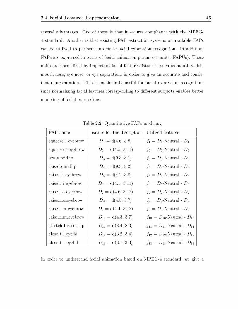
2.4 Facial Features Representation 46
several advantages. One of these is that it secures compliance with the MPEG-
4 standard. Another is that existing FAP extraction systems or available FAPs
can be utilized to perform automatic facial expression recognition. In addition,
FAPs are expressed in terms of facial animation parameter units (FAPUs). These
units are normalized by important facial feature distances, such as mouth width,
mouth-nose, eye-nose, or eye separation, in order to give an accurate and consis-
tent representation. This is particularly useful for facial expression recognition,
since normalizing facial features corresponding to different subjects enables better
modeling of facial expressions.
Table 2.2: Quantitative FAPs modeling
FAP name Feature for the discription Utilized features
squeeze l eyebrow D1 = d(4.6, 3.8) f1 = D1-Neutral - D1
squeeze r eyebrow D2 = d(4.5, 3.11) f2 = D2-Neutral - D2
low t midlip D3 = d(9.3, 8.1) f3 = D3-Neutral - D3
raise b midlip D4 = d(9.3, 8.2) f4 = D4-Neutral - D4
raise l i eyebrow D5 = d(4.2, 3.8) f5 = D5-Neutral - D5
raise r i eyebrow D6 = d(4.1, 3.11) f6 = D6-Neutral - D6
raise l o eyebrow D7 = d(4.6, 3.12) f7 = D7-Neutral - D7
raise r o eyebrow D8 = d(4.5, 3.7) f8 = D8-Neutral - D8
raise l m eyebrow D9 = d(4.4, 3.12) f9 = D9-Neutral - D9
raise r m eyebrow D10 = d(4.3, 3.7) f10 = D10-Neutral - D10
stretch l cornerlip D11 = d(8.4, 8.3) f11 = D11-Neutral - D11
close t l eyelid D12 = d(3.2, 3.4) f12 = D12-Neutral - D12
close t r eyelid D13 = d(3.1, 3.3) f13 = D13-Neutral - D13
In order to understand facial animation based on MPEG-4 standard, we give a

2.4 Facial Features Representation 47
brief description of some keywords of the parameters system.
FAPU(Facial Animation Parameters Units) All animation parameters are
described in FAPU units. This unit is based on face model proportions and
computed based on a few key points of the face (like eye distance or mouth
size).
FDP(Facial Definition Parameters) This acronym describes a set of 88 fea-
ture points of the face model. FAPU and facial animation parameters are
based on these feature points.
FAP(Facial Animation Parameters) It is a set of values decomposed in high
level and low level parameters that represent the displacement of some fea-
tures points (FP) according to a specific direction.
We select the feature displacement and velocity approach due to its suitability for
a real-time video system, in which motion is inherent and which places a strict
upper bound on the computational complexity of methods used in order to meet
time constraints.
Although FAPs are practical and very useful for animation purpose, they are inad-
equate for analyzing facial expressions from video scenes or still images. The main
reason is the absence of quantitative definitions for FAPs as well as their nonad-
ditive nature. In order to measure facial related FAPs in real images and video
sequences, it is necessary to define a way of describing them through the movement
of points that lie in the facial area and that can be automatically detected. Quan-
titative description of FAPs based on particular FDPs points, which correspond
to movement of protuberant facial points, provides the means of bridging the gap
between expression analysis and animation. In the expression analysis case, the
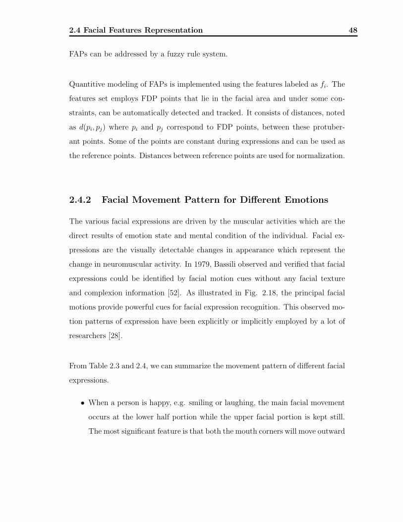
2.4 Facial Features Representation 48
FAPs can be addressed by a fuzzy rule system.
Quantitive modeling of FAPs is implemented using the features labeled as fi. The
features set employs FDP points that lie in the facial area and under some con-
straints, can be automatically detected and tracked. It consists of distances, noted
as d(pi, pj) where pi and pj correspond to FDP points, between these protuber-
ant points. Some of the points are constant during expressions and can be used as
the reference points. Distances between reference points are used for normalization.
2.4.2 Facial Movement Pattern for Different Emotions
The various facial expressions are driven by the muscular activities which are the
direct results of emotion state and mental condition of the individual. Facial ex-
pressions are the visually detectable changes in appearance which represent the
change in neuromuscular activity. In 1979, Bassili observed and verified that facial
expressions could be identified by facial motion cues without any facial texture
and complexion information [52]. As illustrated in Fig. 2.18, the principal facial
motions provide powerful cues for facial expression recognition. This observed mo-
tion patterns of expression have been explicitly or implicitly employed by a lot of
researchers [28].
From Table 2.3 and 2.4, we can summarize the movement pattern of different facial
expressions.
• When a person is happy, e.g. smiling or laughing, the main facial movement
occurs at the lower half portion while the upper facial portion is kept still.
The most significant feature is that both the mouth corners will move outward

2.4 Facial Features Representation 49
Table 2.3: The facial movements cues for six emotions.
Emotion Forehead & eyebrow Eyes Mouth & Nose
Happiness Eyebrows are relaxed Raise upper and lower lids
slightly
Pull back and up lip cor-
ners toward the ears
Sadness Bend together and upward
the inner eyebrows
Drop down upper lids
Raise lower lids slightly
Extend mouth
Fear Raise brows and pull to-
gether
Eyes are tense and alert Slightly tense mouth and
draw back
Bent upward inner eye-
brows
May open mouth
Disgust Lower the eyebrows Push up lids without tense Lips are curled and often
asymmetrical
Surprise Raise eyebrows Drawn down lower eyelid Drop jaw, Open mouth
Horizontal wrinkles Raise upper eyelid No tension or stretching of
the mouth
Anger Lower and draw together
eyebrows
Eyes have a hard stare
Tense upper and lower lids
Mouth firmly pressed Nos-
trils may be dilated
Vertical wrinkles between
eyebrows

2.4 Facial Features Representation 50
0X
Y
Figure 2.17: The facial coordinates.
and toward the ear. Sometimes, when laughing, the jaw will drop and mouth
will be open.
• When a sad expression occur, the eyebrows will bend together and upward a
bit at the inner parts. The mouth will extend. At the same time, the upper
lids may drop down and lower lids may raise slightly.
• The facial moving features of the fear expression mainly occur at the eye and
mouth portion. The eyebrows may raise and pull together. The eyes will
become tense and alert. The mouth will also tend to be tense and may draw
back and open.
• When a person is disgusted about something, the lips will be curled and often
asymmetrical.
• The surprise expression has the most widely spread features. The whole
eyebrows will bend upward and horizontal wrinkles may occur as a result
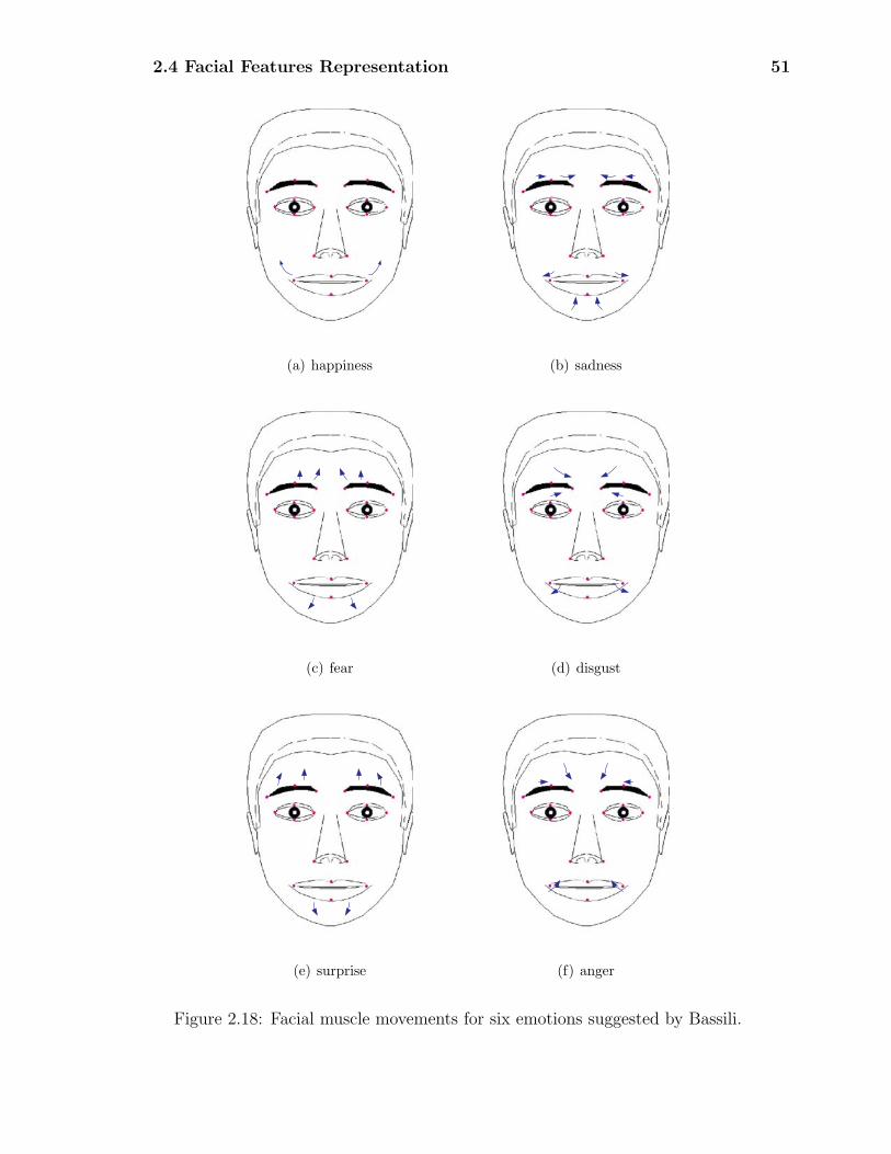
2.4 Facial Features Representation 51
(a) happiness (b) sadness
(c) fear (d) disgust
(e) surprise (f) anger
Figure 2.18: Facial muscle movements for six emotions suggested by Bassili.

2.4 Facial Features Representation 52
of the eyebrow raise. The eyelids will move oppositely and the eyes will be
open. Jaw will drop and mouth may open largely.
• When a person is in anger, the eyebrows are lowered and drawn together.
Vertical wrinkles may appear between eyebrows. The eyes have a hard stare
and both lids are tense. The mouth may be firmly pressed.

2.4 Facial Features Representation 53
Table 2.4: The movements clues of facial features for six emotions
Features Points Happiness Sadness Fear Anger Surprise Disgust
LeftEyeBrowInner ↑ → ↑ → ↑ →
LeftEyeBrowOuter ↑ ↑ →
LeftEyeBrowMiddle ↑ ↓ ↑ ↓ ↑
RightEyeBrowInner ↑ ← ↑ ← ↑ ←
RightEyeBrowOuter ↑ ↑ ←
RightEyeBrowMiddle ↑ ↓ ↑ ↓ ↑
LeftEyeInnerCorner
LeftEyeOuterCorner ←
LeftEyeUpper ↑ ↓ ↑ ↓ ↑
LeftEyeLower ↓ ↓ ↑ ↓
RightEyeInnerCorner
RightEyeOuterCorner →
RightEyeUpper ↑ ↓ ↑ ↓ ↑
RightEyeLower ↓ ↓ ↑ ↓
LeftMouthCorner ↖ ↙ ↙
RightMouthCorner ↗ ↘ ↘
UpperMouth ↑ ↑ ↑ ↑
LowerMouth ↓ ↓ ↑ ↓
Chapter 3Nonlinear Dimension Reduction (NDR)
Methods
To analyze faces in images efficiently, dimensionality reduction is an important
and necessary operation for multi-dimensional image data. The goal of dimen-
sionality reduction is to discover the intrinsic property of the expression data. A
more compact representation of the original data can be obtained which nonethe-
less captures all the information necessary for higher-level decision-making. The
reasons for reducing the dimensionality can be summarized as: (i) To reduce stor-
age requirements; (ii) To eliminate noise; (iii) To extract features from data for
face detection; and (iv) To project data to a lower-dimensional space, especially a
visualized space, so as to be able to discern data distribution [53]. For facial expres-
sion analysis, classical dimensionality reduction methods have included Eigenfaces
[10], Principal Component Analysis (PCA) [5], Independent Component Analysis
(ICA) [54], Multidimensional Scaling (MDS) [55] and Linear Discriminate Analy-
sis (LDA) [56]. However, these methods all have serious drawbacks, such as being
unable to reveal the intrinsic distribution of a given data set, or inaccuracies in de-
tecting faces that exhibit variations in head pose, facial expression or illumination.
54
3.1 Image Vector Space 55
The facial image data are always high-dimensional and require considerable com-
puting time for classification. Face images are regarded as a nonlinear manifold
in high-dimensional space. PCA and LDA are two powerful tools utilized for data
reduction and feature extraction in face recognition approaches. Linear methods
like PCA and LDA are bounds to ignore essential nonlinear structures that are con-
tained in the manifold. Nonlinear dimension reduction methods, such as ISOMAP
[57], Locally Linear Embedding (LLE) [58] method etc. are presented in recent
years.
The high dimensionality of the raw data would be an obstacle for direct analysis.
Therefore, dimension reduction is critical for analyzing the images, to compress the
information and to discover compact representations of variability. In this chap-
ter, we modify the LLE algorithm and propose a new Distributed Locally Linear
Embedding (DLLE) to discover the inherent properties of the input data. By esti-
mating the probability density function of the input data, an exponential neighbor
finding method is proposed. Then the input data are mapped to low dimension
where not only the local neighborhood relationship but also global distribution
are preserved [59]. Because the DLLE can preserve the neighborhood relationships
among input samples, after embedded in low-dimensional space, the 2D embedding
could be much easier for higher-level decision-making.
3.1 Image Vector Space
The human face image can be seen as a set of high dimensional values. A movement
of facial muscle will result in different images. The similarity between two images
can be extracted by comparing the pixel values. An image of a subject’s facial
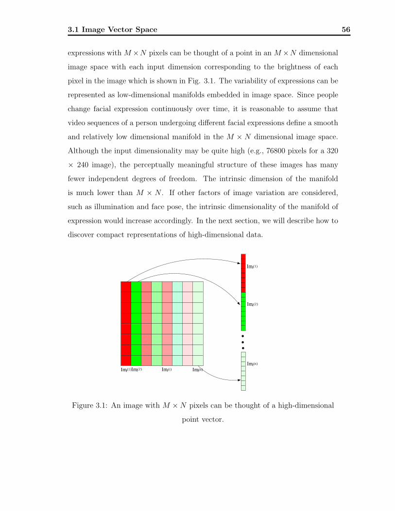
3.1 Image Vector Space 56
expressions with M ×N pixels can be thought of a point in an M ×N dimensional
image space with each input dimension corresponding to the brightness of each
pixel in the image which is shown in Fig. 3.1. The variability of expressions can be
represented as low-dimensional manifolds embedded in image space. Since people
change facial expression continuously over time, it is reasonable to assume that
video sequences of a person undergoing different facial expressions define a smooth
and relatively low dimensional manifold in the M × N dimensional image space.
Although the input dimensionality may be quite high (e.g., 76800 pixels for a 320
× 240 image), the perceptually meaningful structure of these images has many
fewer independent degrees of freedom. The intrinsic dimension of the manifold
is much lower than M × N . If other factors of image variation are considered,
such as illumination and face pose, the intrinsic dimensionality of the manifold of
expression would increase accordingly. In the next section, we will describe how to
discover compact representations of high-dimensional data.
Imi(1)Imi(2) Imi(n)Imi(i)
Imi(1)
Imi(2)
Imi(n)
Figure 3.1: An image with M ×N pixels can be thought of a high-dimensional
point vector.
3.2 LLE and NLE 57
3.2 LLE and NLE
For ease of the forthcoming discussion, we first introduce the main features of LLE
and NLE methods. LLE is an unsupervised learning algorithm that attempts to
map high-dimensional data to low-dimensional space while preserving the neigh-
borhood relationship. Compared to principle component analysis (PCA) and mul-
tidimensional scaling (MDS), LLE is for nonlinear dimensionality reduction. It is
based on simple geometric intuitions: (i) each high dimensional data point and its
neighbors lie on or close to a locally linear patch of a manifold, and (ii) the local
geometric characterization in original data space is unchanged in the output data
space. The neighbor finding process of each data point of LLE is: for each data
point in the given data set, using the group technique such as K nearest neigh-
bors based on the Euclidean distance, the neighborhood for any given point can
be found. A weighted graph is set up with K nodes, one for each neighbor point,
and a set of edges connecting neighbor points. These neighbors are then used to
reconstruct the given point by linear coefficients.
In order to provide a better basis for structure discovery, NLE [60] is proposed. It
is an adaptive scheme that selects neighbors according to the inherent properties of
the input data substructures. The neighbor finding procedure of NLE for a given
point xi, by defining dij the Euclidean distance from node xj to xi and Si the data
set containing all the neighbor indices of xi, can be summarized as follows:
• If dij = min{dim}, ∀ m ∈ 1, 2,..., N, then xj is regarded as a neighbor of the
node xi. Initial Si = {xj}
• Provided that xk is the second nearest node to node xi, xk is a neighbor of
3.2 LLE and NLE 58
node xi if the following two inequations is satisfied.
Si =
⎧⎪⎨⎪⎩
Si ∪ {xk}, if djk > dik
Si, otherwise
• If Si contains two or more elements, that is card(Si) ≥ 2, if ∀ m ∈ Si, the
following two inequations hold:
⎧⎪⎨⎪⎩
djm > dji
djm > dmi
then Si = Si ∪ {xm}”
Both LLE and NLE methods can find the inherent embedding in low dimension.
According to the LLE algorithm, each point xi is only reconstructed from its K
nearest neighbors by linear coefficients. However, due to the complexity, nonlinear-
ity and variety of high dimensional input data, it is difficult to use a fixed K for all
the input data to find the intrinsic structure [61]. The proper choice of K affects
an acceptable level of redundancy and overlapping. If K is too small or too large,
the K-nearest neighborhood method cannot properly approximate the embedding
of the manifold. The size of range depends on various features of the data, such as
the sampling density and the manifold geometry. An improvement can be done by
adaptively selecting neighbor number according to the density of the sample points.
Another problem of using K nearest neighbors is the information redundancy. As
illustrated in Fig. 3.2, e.g., for a certain manifold, we choose K(K = 8) nearest
neighbors to reconstruct xi. However, the selected neighbors in the dashed circle
are closely gathered. Obviously, if we use all of samples in the circle as the neighbors
of xi, the information captured in that direction will have somewhat redundancy.
A better straightforward way is to use one or several samples to represent a group
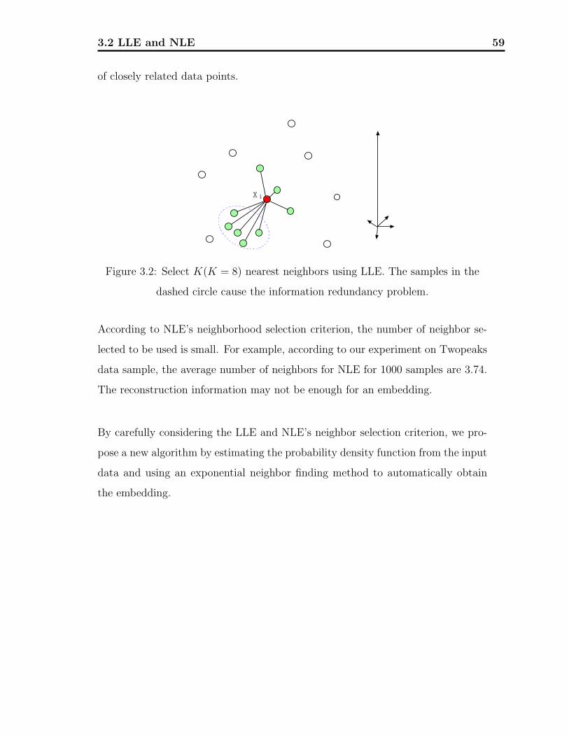
3.2 LLE and NLE 59
of closely related data points.
X i
Figure 3.2: Select K(K = 8) nearest neighbors using LLE. The samples in the
dashed circle cause the information redundancy problem.
According to NLE’s neighborhood selection criterion, the number of neighbor se-
lected to be used is small. For example, according to our experiment on Twopeaks
data sample, the average number of neighbors for NLE for 1000 samples are 3.74.
The reconstruction information may not be enough for an embedding.
By carefully considering the LLE and NLE’s neighbor selection criterion, we pro-
pose a new algorithm by estimating the probability density function from the input
data and using an exponential neighbor finding method to automatically obtain
the embedding.
3.3 Distributed Locally Linear Embedding (DLLE) 60
3.3 Distributed Locally Linear Embedding (DLLE)
3.3.1 Estimation of Distribution Density Function
In most cases, a prior knowledge of the distribution of the samples in high dimen-
sion space is not available. However, we can estimate a density function of the
given data. Consider a data set with N elements in m dimensional space, for each
sample xi, the approximated distribution density function pxiaround point xi can
be calculated as:
pxi=
ki∑N1 ki
(3.1)
where ki is number of the points within a hypersphere kernel of fixed radius around
point xi.
Let P = {px1 , px2 , · · · , pxN} denote the set of estimated distribution density func-
tion, pmax=max(P ) and pmin=min(P ).
3.3.2 Compute the Neighbors of Each Data Point
Suppose that a data set X = {x1, x2, · · · , xn}, xi ∈ Rm is globally mapped to a
data set Y = {y1, y2, · · · , yn}, yi ∈ Rl, m � l. For the given data set, each data
point and its neighbors lie on or close to a locally linear patch of the manifold.
The neighborhood set of xi, Si (i = 1, ..., N) can be constructed by making use of
the neighborhood information.
Assumption 4. Suppose that the input data set X contains sufficient data in Rm
sampled from a smooth parameter space Φ. Each data point xi and its neighbors
e.g. xj, to lie on or close to a roughly linear patch on the manifold. The range of
this linear patch is subject to the estimated sampling density p and mean distances
3.3 Distributed Locally Linear Embedding (DLLE) 61
d from other points in the input space.
Based on above geometry conditions, the local geometry in the neighborhood of
each data point can be reconstructed from its neighbors by linear coefficients. At
the same time, the mutual reconstruction information depends on the distance
between the points. The larger the distance between points, the little mutual re-
construction information between them.
Assumption 5. The parameter space Φ is a convex subset of Rm. If xi and xj
is a pair of points in Rm, φi and φj is the corresponding points in Φ, then all the
points defined by {(1− t)φi + tφj : t ∈ (0, 1)} lies in Φ.
In view of the above observations, the following procedure is conducted making
use of the neighbor information to construct the reconstruction data set of xi,
Si (i = 1, ..., N). To better sample the near neighbor and the outer data points, we
propose an algorithm using an exponential format to gradually enlarge the range
to find the reconstruction sample.
For a given point xi, we can compute the distances from all other points around
it. According to the distribution density function around xi estimated before, we
introduce αi to describe the normalized density of the sample point xi and is used
to control the increment of the segment according to the sample points density for
neighbor selection. We first give the definition of αi by normalizing pxiusing the
estimated distribution density function computed by equation (3.1):
αi = β · pmax − pxi
pmax − pmin
+ α0 (3.2)
where β is scaling constant, default value is set to 1.0; α0 is the constant to be set.
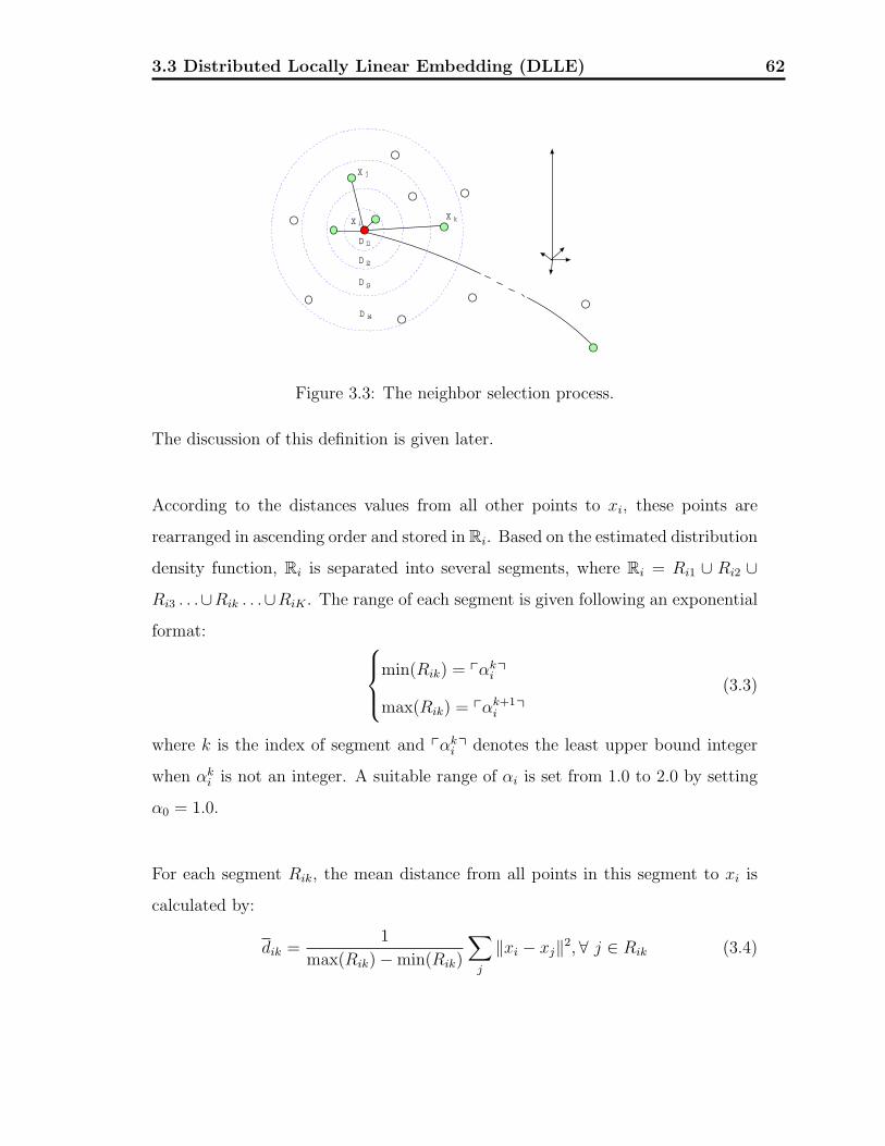
3.3 Distributed Locally Linear Embedding (DLLE) 62
X i
D i1
D i2
D i3
D i4
X j
X k
Figure 3.3: The neighbor selection process.
The discussion of this definition is given later.
According to the distances values from all other points to xi, these points are
rearranged in ascending order and stored in Ri. Based on the estimated distribution
density function, Ri is separated into several segments, where Ri = Ri1 ∪ Ri2 ∪Ri3 . . .∪Rik . . .∪RiK . The range of each segment is given following an exponential
format: ⎧⎪⎨⎪⎩
min(Rik) = �αki �
max(Rik) = �αk+1i �
(3.3)
where k is the index of segment and �αki � denotes the least upper bound integer
when αki is not an integer. A suitable range of αi is set from 1.0 to 2.0 by setting
α0 = 1.0.
For each segment Rik, the mean distance from all points in this segment to xi is
calculated by:
dik =1
max(Rik)−min(Rik)
∑j
‖xi − xj‖2,∀ j ∈ Rik (3.4)
3.3 Distributed Locally Linear Embedding (DLLE) 63
To overcome the information redundancy problem, using the mean distance com-
puted by equation (3.4), we find the most suitable point in Rik to represent the
contribution of all points in Rik by minimizing the following cost equation:
ε(d) = min‖dik − xj‖2, ∀ j ∈ Rik (3.5)
To determine the number of neighbors to be used for further reconstruction and
achieve adaptive neighbor selection, we can compute the mean distance from all
other samples to xi
di =1
N
N∑j=1
‖xi − xj‖2, i �= j (3.6)
Starting with the Si computed above at given point xi, from the largest element
in Si, remove the element one by one until all elements in Si is less than the mean
distance di computed by equation (3.6). Then the neighbor set Si for point xi is
fixed.
3.3.3 Calculate the Reconstruction Weights
The reconstruction weight W is used to rebuild the given point. To store the
neighborhood relationship and reciprocal contributions to each other, the sets Si
(i = 1, 2, ..., N) are converted to a weight matrix W = wij (i, j = 1, 2, ..., N). The
construction weight W that best represents the given point xi from its neighbor xj
is computed by minimizing the cost function given below:
ε(W ) =N∑i
‖xi −Si(ni)∑
j=Si(1)
wijxj‖2, i �= j (3.7)
where the reconstruction weight wij represents the contribution of the jth data
point to the ith point’s reconstruction. The reconstruction weight wij is subjected
to two constraints. First, each data point xi is reconstructed only from its neigh-
borhood set points, enforcing wij = 0 if xj is not its neighbor. Second, the rows of
3.3 Distributed Locally Linear Embedding (DLLE) 64
the weight matrix sum to one.
To compute W row by row, equation (3.7) can be further written as:
ε(Wi) = ‖xi −Si(ni)∑
j=Si(1)
wijxj‖2, i �= j
= ‖Si(ni)∑
j=Si(1)
wijxi −Si(ni)∑
j=Si(1)
wijxj‖2
=
Si(ni)∑j=Si(1)
wij
Si(ni)∑k=Si(1)
wik(xi − xj)T (xi − xj) (3.8)
where Wi is the ith row of W . By defining a local covariance
Ci(j, k) = (xi − xj)(xi − xk)
combined with the constraint of W , we can apply Lagrange multiplier and have
[60]:
ε(Wi) =
Si(ni)∑j=Si(1)
wij
Si(ni)∑k=Si(1)
wikCi(j, k) + ηi(
Si(ni)∑j=Si(1)
wij − 1) (3.9)
where ηi is the Lagrange coefficient. To obtain the minimum of ε, we can find the
partial differentiation with respect to each weight and set it to zero
∂ε(Wi)
∂wij
= 2
Si(ni)∑k=Si(1)
wikCi(Si(j), k) + ηi = 0, ∀j ∈ ui (3.10)
Rewrite equation (3.10) as
C ·W Ti = q (3.11)
where C = {Cjk}(j, k = 1, ..., ni) is a symmetric matrix with dimension ni × ni,
Cjk = Ci(Si(j),Si(k)), and
Wi = [wiSi(1), wiSi(2), · · · , wiSi(ni)], (3.12)
3.3 Distributed Locally Linear Embedding (DLLE) 65
q = [q1, q2, . . . , qni] and qi = ηi/2. If ni > l, the covariance matrix C might be
singular. When in such situation, we can modify the C a bit by C = C + μI,
where μ is a small positive constant. Therefore, Wi can be obtained from equation
(3.12)
W Ti = C−1q (3.13)
The constrained weights of equation obey an important symmetry that they are
invariant to rotation, resealing, and translation for any particular data point and
its neighbors. Thus, W is a sparse matrix that contains the information about
the neighborhood relationship represented spatially by the position of the non-
zero elements in the weight matrix and the contribution of one node to another
represented numerically by their values. The construction of Si and W is detailed
in Algorithm 1.
3.3.4 Computative Embedding of Coordinates
Finally, we find the embedding of the original data set in the low-dimensional space,
e.g. l dimension. Because of the invariance property of reconstruction weights wij,
the weights reconstructing the ith data point in m dimensional space should also
reconstruct the ith data point in l dimensional space. Similarly, this is done by
trying to preserve the geometric properties of the original space by selecting l
dimensional coordinates yi to minimize the embedding function given below:
Φ(Y ) =N∑i
‖yi −Si(ni)∑
j=Si(1)
wijyj‖2
=N∑i
‖Y (Ii −Wi)‖2 (3.14)
= tr(Y (Ii −Wi)(Y (Ii −Wi))T )
= tr(Y MY T )

3.3 Distributed Locally Linear Embedding (DLLE) 66
Algorithm 1 W = NeighborFind(X)
1: Compute D from X D={dij} is the distance matrix
2: Sort D along each column to form D
3: for i← 1, N do
4: for k ← 1, K do
5: if αk < N then
6: min(Dik) = �αk� + k − 1
7: max(Dik) = �αk+1� + k
8: else αk > N
9: break
10: end if
11: dik ← α, k, Dik by solving equation(3.4)
12: xj = arg minxj∈Dik
‖dik − xj‖2
13: Si = Si ∪ {xj}14: ni = ni + 1
15: end for
16: di = 1N
Di
17: if xj > di then
18: Si = Si − {xj}19: ni = ni − 1
20: end if
21: end for
3.3 Distributed Locally Linear Embedding (DLLE) 67
where wij are the reconstruction weights computed in Section 3.3.3, yi and yj are
the coordinates of the point xi and its neighbor xj in the embedded space.
Equation (3.14) can be rearranged as the inner products, (yi · yj), we rewrite it as
the quadratic form:
Φ(Y ) =∑ij
mij(yi · yj) (3.15)
where M = {mij} is an N ×N matrix given by
mij = δij − wij − wji +∑
k
wkiwkj (3.16)
and δij is the Kronecker delta.
Equation (3.16) can be solved as an eigenvector problem by forcing the embedding
outputs to be centered at the origin with the following constraint:
∑i
yi = 0 (3.17)
To force the embedding coordinates to have unit covariance by removing rotational
degree of freedom, the out products must satisfy:
1
N
∑i
yiyTi = I (3.18)
where I is the d× d identity matrix. Optimal embedding coordinates are given by
the bottom d + 1 nonzero eigenvectors of M for the desired dimensionality.
The lower complexity of the embedded motion curve allows a rather simple geo-
metric tool to analyze the curve in order to disclose significant points. In the next
section, we explore the space of expression through the manifold of expression. The
analysis of the relationships between different facial expressions will be facilitated
on the manifold.

3.4 LLE, NLE and DLLE comparison 68
−1
−0.5
0
0.5
1
−1
−0.5
0
0.5
1−1
−0.5
0
0.5
1
(a) Twopeaks (b) LLE
(c) NLE (d) DLLE
Figure 3.4: Twopeaks
3.4 LLE, NLE and DLLE comparison
For the comparison of the embedding property, we have conducted several manifold
learning algorithms as well as several testing examples. Here we mainly illustrate
three algorithms LLE, NLE and DLLE graphicly using two classical data sets: two
peaks and punched sphere. For each data set, each method was used to obtain
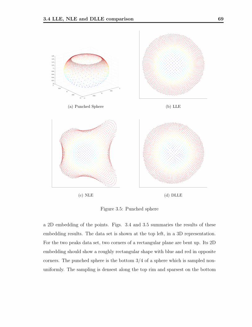
3.4 LLE, NLE and DLLE comparison 69
−1
−0.5
0
0.5
1
−1
−0.5
0
0.5
10
0.2
0.4
0.6
0.8
1
1.2
1.4
1.6
1.8
(a) Punched Sphere (b) LLE
(c) NLE (d) DLLE
Figure 3.5: Punched sphere
a 2D embedding of the points. Figs. 3.4 and 3.5 summaries the results of these
embedding results. The data set is shown at the top left, in a 3D representation.
For the two peaks data set, two corners of a rectangular plane are bent up. Its 2D
embedding should show a roughly rectangular shape with blue and red in opposite
corners. The punched sphere is the bottom 3/4 of a sphere which is sampled non-
uniformly. The sampling is densest along the top rim and sparsest on the bottom

3.4 LLE, NLE and DLLE comparison 70
of the sphere. Its intrinsic structure should be 2D concentric circles. Both the
sample data sets were constructed by sampling 2000 points.
In Fig. 3.4, as expected, all the three algorithms can correctly embed the blue
and red samples in opposite corners. However, the outline shape of the embedding
using NLE is distorted when projected in 2D. DLLE can give a better preservation
of the global shape of the original rectangle compared to LLE. At the same time,
the green samples perform as the inner and outer boundary are also well kept using
DLLE.
As can be seen in Fig. 3.5, both DLLE and LLE are successful in flattening the
punched sphere and recover all the original concentric circles. NLE seems to be
confused about the heavy point density around the rim. It can preserve the inner
circles well but fails on the outer circle because of its neighbors selection criterion.
Chapter 4Facial Expression Energy
Each person has his/her own maximal intensity of displaying a particular expres-
sion. There is a maximal energy pattern for each person for their respective facial
expression. Therefore, facial expression energy can be used for classification by
adjusting the general expression pattern to a particular individual according to
the individual’s successful expression recognition results.
Matsuno et al. presented a method from an overall pattern of the face which is
represented in a potential field activated by edges in the image for recognition [62].
In [22], Essa et al. proposed motion energy template where the authors use the
physics-based model to generate spatio-temporal motion energy template for each
expression. The motion energy is converted from muscles activations. However,
the authors did not provide a definition for motion energy. At the same time,
they only used the spatial information in their recognition pattern. In this the-
sis, we firstly give out a complete definition of facial expression potential energy
and kinetic energy based on the facial features’ movements information. A facial
expression energy system is built up to describe the muscles’ tension in facial ex-
pression for classification. By further considering different expressions’ temporal
71

4.1 Physical Model of Facial Muscle 72
transition characteristics, we are able to pin-point the actual occurrence of specific
expressions with higher accuracy.
4.1 Physical Model of Facial Muscle
Muscles are a kind of soft tissues that possess contractile properties. Facial surface
deformation during an expression is triggered by the contractions of the synthetic
facial muscles. The muscle forces are propagated through the skin layer and fi-
nally deform the facial surface. A muscle can contract more forcefully when it is
slightly stretched. Muscle generates maximal concentric tension beyond its phys-
iological range-at a length 1.2 times its resting length. Beyond this length, active
tension decreases due to insufficient sarcomere overlap. To simulate muscle forces
and the dynamics of muscle contraction, mass-spring model is typically utilized
[63, 64, 65]. Waters and Frisble [66] proposed a two-dimensional mass-spring model
of the mouth with the muscles represented as bands.
A mass-spring model used to construct a face mask is shown in Fig. 4.1 [67]. Each
node in the model is regarded as a particle with mass. The connection between
two nodes is modeled by a spring. The spring force is proportional to the change
of spring length according to the Hooke’s law. The node in the model can move to
the position until it arrives at the equilibrium point.
The facial expression energy is computed by “compiling” the detailed, physical
model of facial feature movements into a set of biologically motion energy. This

4.2 Emotion Dynamics 73
Figure 4.1: The mass spring face model [67].
method takes advantage of the optical flow which tracks the feature points’ move-
ments information. For each expression, we use the facial feature movements in-
formation to compute the typical pattern of motion energy. These patterns are
subsequently used for expression recognition.
4.2 Emotion Dynamics
Fig. 4.2 shows some preprocessed and cropped example images for a happy expres-
sion. As illustrated in the example, all acquired sequences start from the neutral
state passing into the emotional state and end with a neutral state.
One common limitation of the existing works is that the recognition is performed
by using static cues from still face images without considering the temporal be-
havior of facial expressions. The psychological experiments by Bassili [52] have
suggested that facial expressions are more accurately recognized from a dynamic
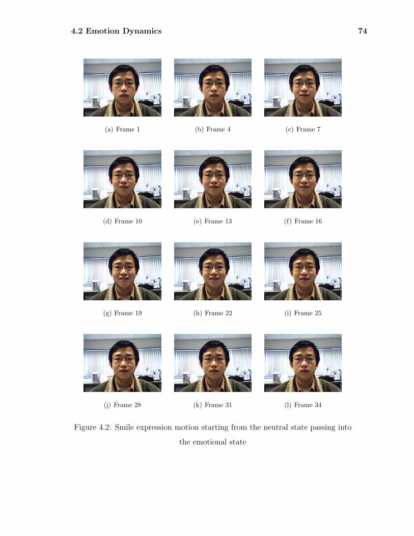
4.2 Emotion Dynamics 74
(a) Frame 1 (b) Frame 4 (c) Frame 7
(d) Frame 10 (e) Frame 13 (f) Frame 16
(g) Frame 19 (h) Frame 22 (i) Frame 25
(j) Frame 28 (k) Frame 31 (l) Frame 34
Figure 4.2: Smile expression motion starting from the neutral state passing into
the emotional state
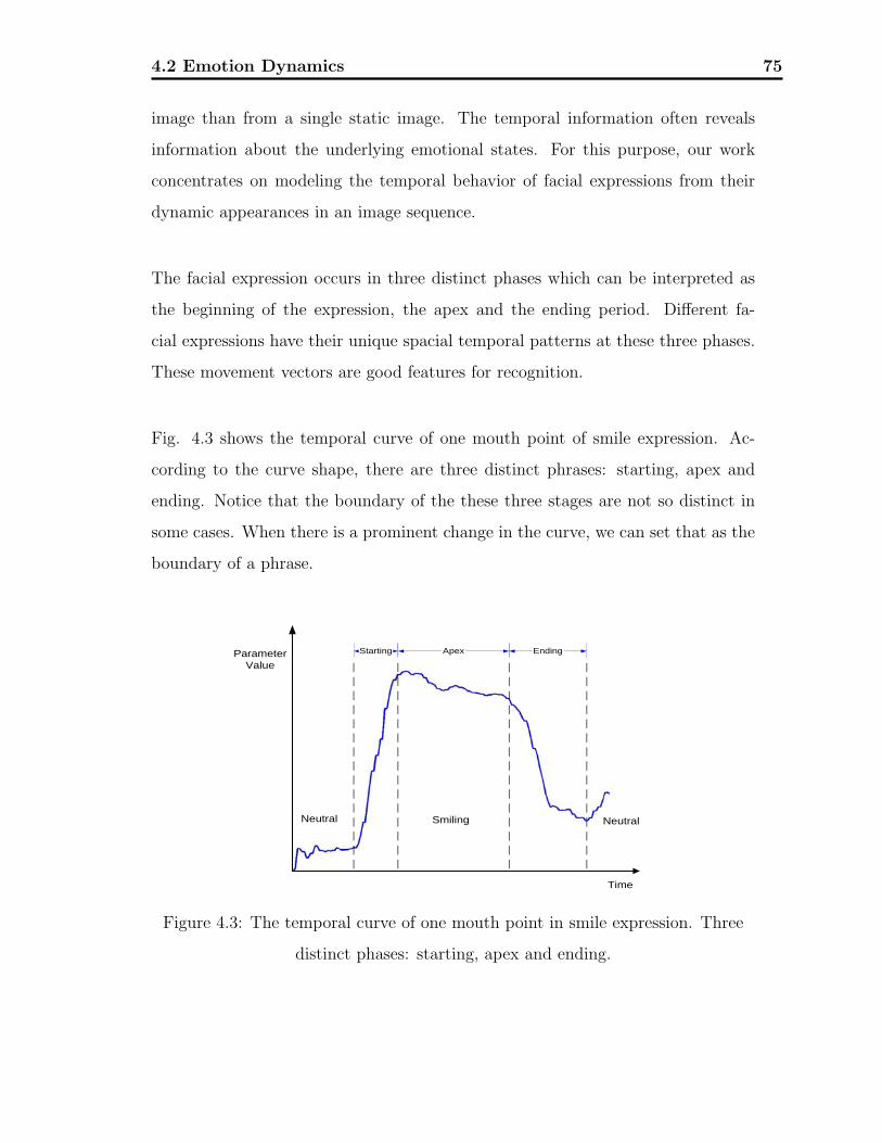
4.2 Emotion Dynamics 75
image than from a single static image. The temporal information often reveals
information about the underlying emotional states. For this purpose, our work
concentrates on modeling the temporal behavior of facial expressions from their
dynamic appearances in an image sequence.
The facial expression occurs in three distinct phases which can be interpreted as
the beginning of the expression, the apex and the ending period. Different fa-
cial expressions have their unique spacial temporal patterns at these three phases.
These movement vectors are good features for recognition.
Fig. 4.3 shows the temporal curve of one mouth point of smile expression. Ac-
cording to the curve shape, there are three distinct phrases: starting, apex and
ending. Notice that the boundary of the these three stages are not so distinct in
some cases. When there is a prominent change in the curve, we can set that as the
boundary of a phrase.
EndingApexStarting
Time
ParameterValue
Neutral Smiling Neutral
Figure 4.3: The temporal curve of one mouth point in smile expression. Three
distinct phases: starting, apex and ending.

4.3 Potential Energy 76
4.3 Potential Energy
Expression potential energy is the energy that is stored as a result of deformation
of a set of muscles. It would be released if a facial expression in a facial potential
field was allowed to go back from its current position to an equilibrium position
(such as the neutral position of the feature points). The potential energy may be
defined as the work that must be done in the facial expression, the muscles’ force
so as to achieve that configuration. Equivalently, it is the energy required to move
the feature point from the equilibrium position to the given position. Considering
the contractile properties of muscles, this definition is similar to the elastic po-
tential energy. It is defined as the work done by the muscle’s elastic force. For
example, the mouth corner extended at the extreme position has greater facial po-
tential energy than the same corner extended a bit. To move the mouth corner to
the extreme position, work must be done, with energy supplied. Assuming perfect
efficiency (no energy losses), the energy supplied to extend the mouth corner is
exactly the same as the increase of its facial potential energy. The mouth corner’s
potential energy can be released by relaxing the facial muscle when the expression
is to the end. As the facial expression fades out, its potential energy is converted
to kinetic energy.
For each expression, there is a typical pattern of muscle actuation. The corre-
sponding feature movement pattern can be tracked and determined using optical
flow analysis. Typical pattern of motion energy can be generated and associated
with each facial expression. This results in a set of simple expression “detectors”
each of which looks for the particular space-time pattern of motion energy associ-
ated with each facial expression.
According to the captured features’ displacements using Lucas and Kanade(L-K)
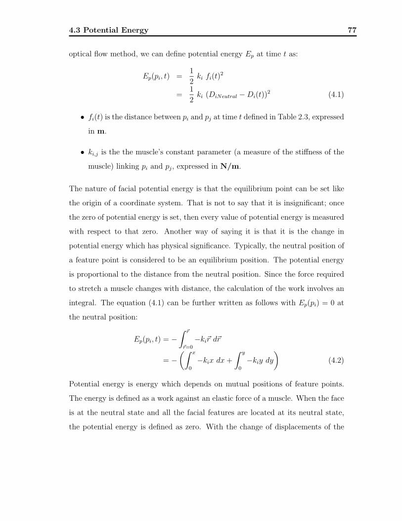
4.3 Potential Energy 77
optical flow method, we can define potential energy Ep at time t as:
Ep(pi, t) =1
2ki fi(t)
2
=1
2ki (DiNeutral −Di(t))
2 (4.1)
• fi(t) is the distance between pi and pj at time t defined in Table 2.3, expressed
in m.
• ki,j is the the muscle’s constant parameter (a measure of the stiffness of the
muscle) linking pi and pj, expressed in N/m.
The nature of facial potential energy is that the equilibrium point can be set like
the origin of a coordinate system. That is not to say that it is insignificant; once
the zero of potential energy is set, then every value of potential energy is measured
with respect to that zero. Another way of saying it is that it is the change in
potential energy which has physical significance. Typically, the neutral position of
a feature point is considered to be an equilibrium position. The potential energy
is proportional to the distance from the neutral position. Since the force required
to stretch a muscle changes with distance, the calculation of the work involves an
integral. The equation (4.1) can be further written as follows with Ep(pi) = 0 at
the neutral position:
Ep(pi, t) = −∫ �r
�r=0
−ki�r d�r
= −(∫ x
0
−kix dx +
∫ y
0
−kiy dy
)(4.2)
Potential energy is energy which depends on mutual positions of feature points.
The energy is defined as a work against an elastic force of a muscle. When the face
is at the neutral state and all the facial features are located at its neutral state,
the potential energy is defined as zero. With the change of displacements of the
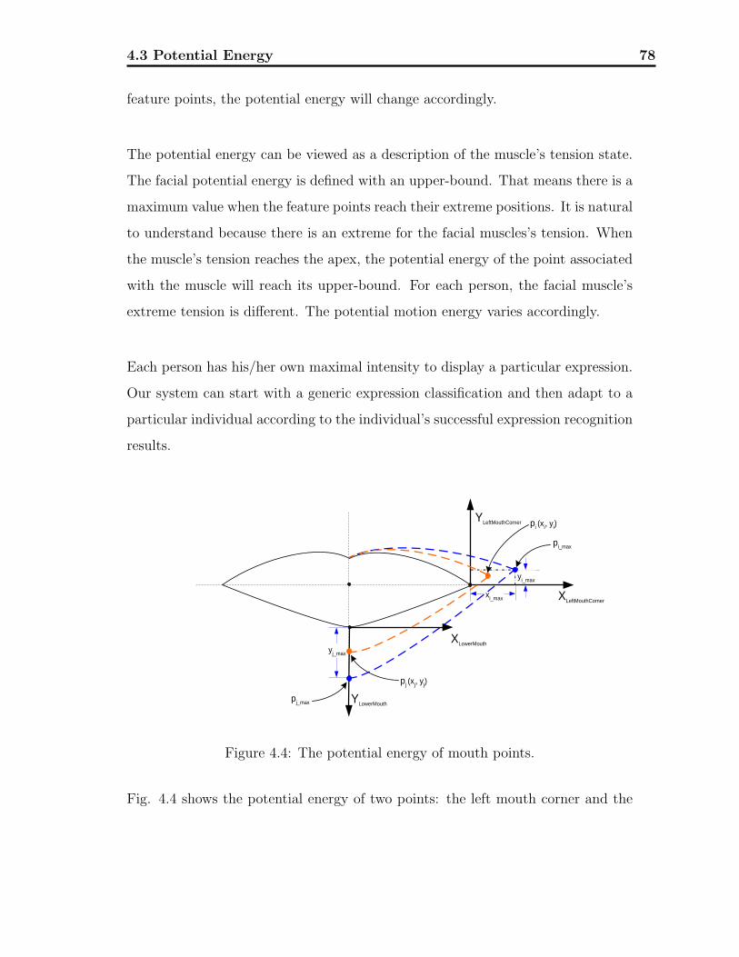
4.3 Potential Energy 78
feature points, the potential energy will change accordingly.
The potential energy can be viewed as a description of the muscle’s tension state.
The facial potential energy is defined with an upper-bound. That means there is a
maximum value when the feature points reach their extreme positions. It is natural
to understand because there is an extreme for the facial muscles’s tension. When
the muscle’s tension reaches the apex, the potential energy of the point associated
with the muscle will reach its upper-bound. For each person, the facial muscle’s
extreme tension is different. The potential motion energy varies accordingly.
Each person has his/her own maximal intensity to display a particular expression.
Our system can start with a generic expression classification and then adapt to a
particular individual according to the individual’s successful expression recognition
results.
yj_max
yi_max
xi_max XLeftMouthCorner
YLeftMouthCorner
XLowerMouth
YLowerMouth
pi (xi, yi)
pj (xj, yj)
pi_max
pj_max
Figure 4.4: The potential energy of mouth points.
Fig. 4.4 shows the potential energy of two points: the left mouth corner and the
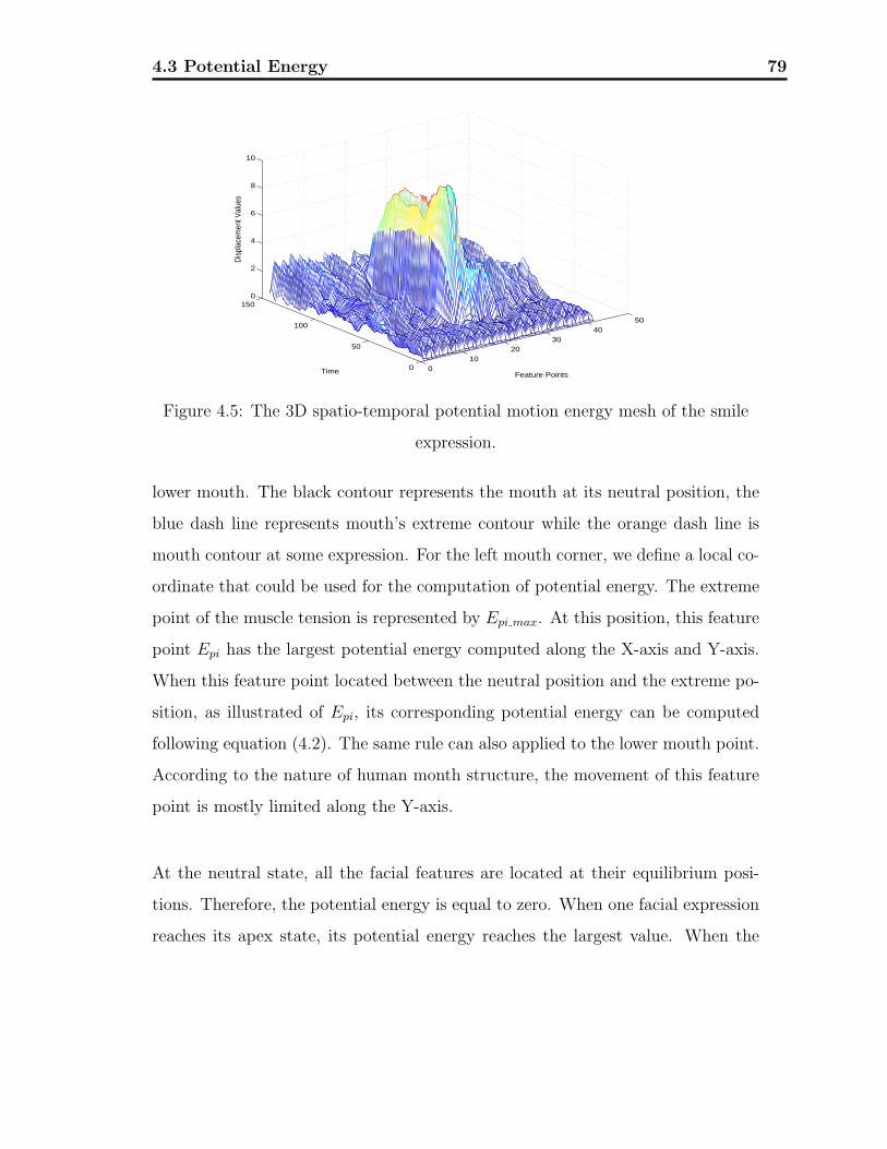
4.3 Potential Energy 79
010
2030
4050
0
50
100
1500
2
4
6
8
10
Feature PointsTime
Dis
plac
emen
t Val
ues
Figure 4.5: The 3D spatio-temporal potential motion energy mesh of the smile
expression.
lower mouth. The black contour represents the mouth at its neutral position, the
blue dash line represents mouth’s extreme contour while the orange dash line is
mouth contour at some expression. For the left mouth corner, we define a local co-
ordinate that could be used for the computation of potential energy. The extreme
point of the muscle tension is represented by Epi max. At this position, this feature
point Epi has the largest potential energy computed along the X-axis and Y-axis.
When this feature point located between the neutral position and the extreme po-
sition, as illustrated of Epi, its corresponding potential energy can be computed
following equation (4.2). The same rule can also applied to the lower mouth point.
According to the nature of human month structure, the movement of this feature
point is mostly limited along the Y-axis.
At the neutral state, all the facial features are located at their equilibrium posi-
tions. Therefore, the potential energy is equal to zero. When one facial expression
reaches its apex state, its potential energy reaches the largest value. When the

4.4 Kinetic Energy 80
expression is at the ending state, the potential energy will decrease accordingly.
Fig. 4.5 shows the 3D spatio-temporal potential motion energy mesh of the smile
expression.
For each facial expression pattern, there are great varieties in the feature points’
movements. Therefore, the potential energy value varies spatially and temporally.
When an expression reaches its apex state, the potential value will also reach its
maximum. Therefore, the pattern can be classified accordingly.
4.4 Kinetic Energy
Kinetic energy is defined as a work of the force accelerating a facial feature points.
It is the energy that a feature point possesses as a result of facial motion. It is a
description energy.
Our system not only considers the displacement of the feature points in one direc-
tion, but also takes the velocity into account as movements pattern for analysis.
The velocity of each feature points is computed frame by frame. It is natural
that the feature points remain nearly static in the initial and apex state. During
the change of the facial expressions, the related feature points’ movements are fast.
By analyzing the moving features’ velocity, we can find the cue of a certain emotion.
According to the velocity obtained from equation (5.16), we can define kinetic
energy Ek as:
Ek(pi, t) =1
2wi‖vi‖2 (4.3)
where wi denote the ith feature point’s weight, vi is the velocity for point i.

4.4 Kinetic Energy 81
For each facial expression pattern, it will occur from the starting, translation and
vanishing. At the neutral state, since the face is static, the kinetic energy is nearly
zero. When the facial expression is at the starting state, the feature points are
moving fast, the kinetic energy will vary temporally–increase first and decrease
later. During this state, the muscle’s biological energy is converted to feature
points’ kinetic energy. The kinetic energy is converted to feature points’ poten-
tial energy. When an expression reaches its apex state, the kinetic energy will
decrease to a stable state. If the facial muscle is still then, the kinetic energy will
decrease to zero. At this time, the potential energy will reach to its apex. When
the expression is at the ending state, feature points will move back to the neutral
positions. Therefore, the kinetic energy will increase first and decrease later again.
By analyzing and setting a set of rules, associated with the potential energy value,
the pattern can be classified accordingly.
At the same time, the feature points’ movement may temporally differ a lot when
an expression occur, e.g. when someone is angry, he may frown first and then
extend his mouth. Therefore, the kinetic energy for each feature points may not
reach the apex concurrently.
We use a normalized dot product similarity metric to compare the differences
between facial expressions. A simple form of similarity metric is the dot product
between two vectors. We employ a normalized dot product as a similarity metric.
Let Xi be the ith feature of the facial expression vector for expression X. Let the
normalized feature vector, be defined as
Xi =Xi√∑m
j X2j
(4.4)

4.4 Kinetic Energy 82
where m is the number of elements in each expression vector. The similarity be-
tween two facial expression vectors, X and Y , for the normalized dot product is
defined to be X · Y , the dot product on the normalized feature vectors.
Chapter 5Facial Expression Recognition
Most of the researches on automated expression analysis perform an emotional
classification. Once the face and its features have been perceived, the next step
of an automated expression analysis system is to recognize the facial expression
conveyed by the face. A set of categories of facial expression, defined by Ekman,
is referred as the six basic emotions [23]. It is based on the cross culture study on
existence of “universal categories of emotional expressions”, the most known and
most commonly used study on the facial expression classification.
To achieve automating facial expression emotional classification is difficult for a
number of reasons. Firstly, there is no uniquely defined description either in terms
of facial actions or in terms of some other universally defined facial codes. Sec-
ondly, it should be feasible to classify the multiple facial expressions. FACS is the
well known study on describing all visually distinguishable facial movements [23].
Based on the selected person-dependent facial expression images in a video, DLLE
is utilized to project the high dimensional data into the low dimensional embed-
ding. After the embedding of input images are represented in a lower dimension,
83
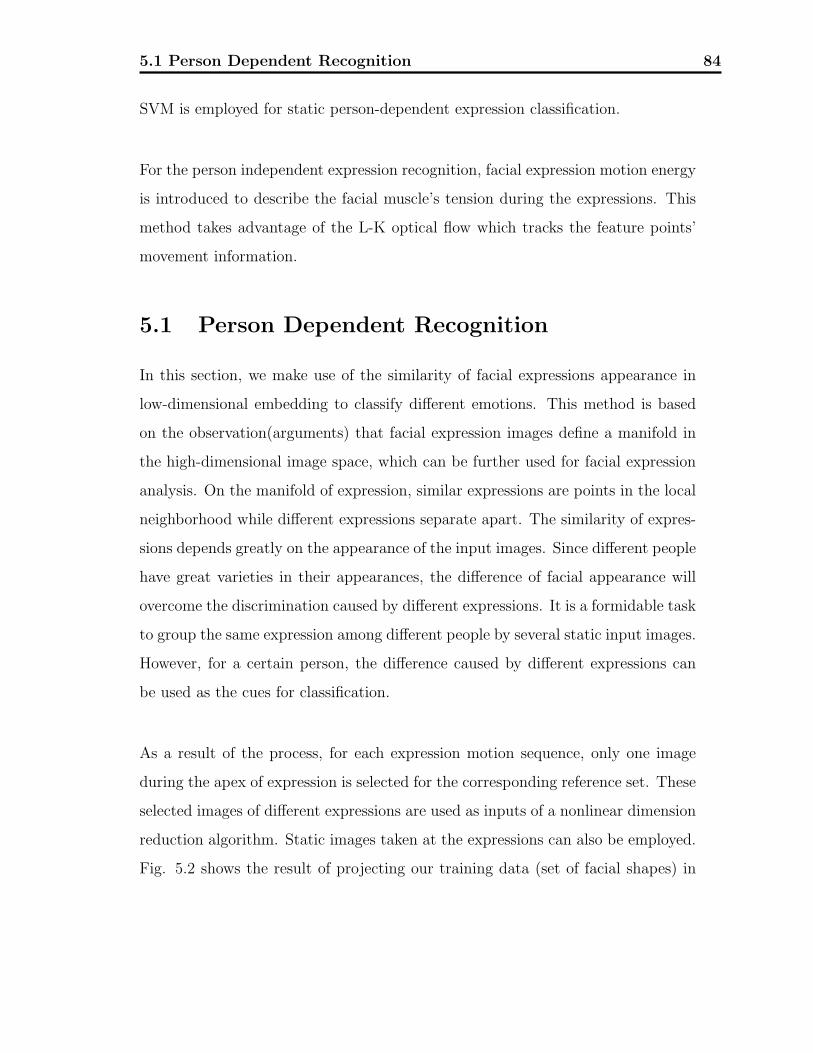
5.1 Person Dependent Recognition 84
SVM is employed for static person-dependent expression classification.
For the person independent expression recognition, facial expression motion energy
is introduced to describe the facial muscle’s tension during the expressions. This
method takes advantage of the L-K optical flow which tracks the feature points’
movement information.
5.1 Person Dependent Recognition
In this section, we make use of the similarity of facial expressions appearance in
low-dimensional embedding to classify different emotions. This method is based
on the observation(arguments) that facial expression images define a manifold in
the high-dimensional image space, which can be further used for facial expression
analysis. On the manifold of expression, similar expressions are points in the local
neighborhood while different expressions separate apart. The similarity of expres-
sions depends greatly on the appearance of the input images. Since different people
have great varieties in their appearances, the difference of facial appearance will
overcome the discrimination caused by different expressions. It is a formidable task
to group the same expression among different people by several static input images.
However, for a certain person, the difference caused by different expressions can
be used as the cues for classification.
As a result of the process, for each expression motion sequence, only one image
during the apex of expression is selected for the corresponding reference set. These
selected images of different expressions are used as inputs of a nonlinear dimension
reduction algorithm. Static images taken at the expressions can also be employed.
Fig. 5.2 shows the result of projecting our training data (set of facial shapes) in
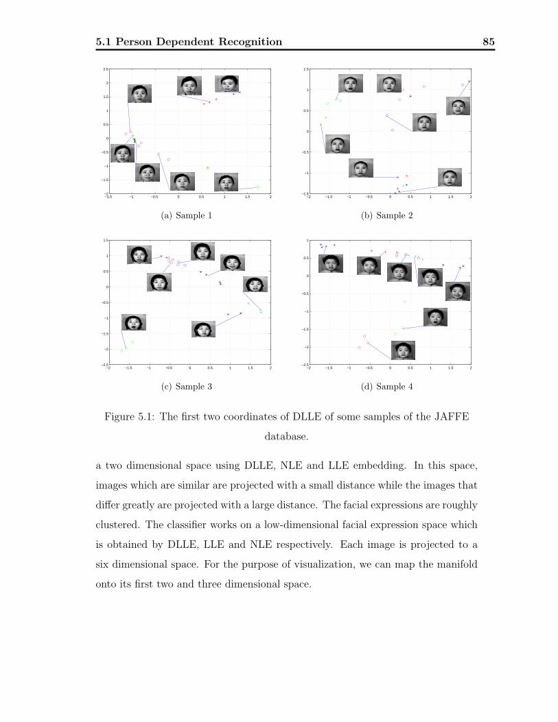
5.1 Person Dependent Recognition 85
−1.5 −1 −0.5 0 0.5 1 1.5 2−2
−1.5
−1
−0.5
0
0.5
1
1.5
2
2.5
(a) Sample 1
−2 −1.5 −1 −0.5 0 0.5 1 1.5 2−1.5
−1
−0.5
0
0.5
1
1.5
(b) Sample 2
−2 −1.5 −1 −0.5 0 0.5 1 1.5 2−2.5
−2
−1.5
−1
−0.5
0
0.5
1
1.5
(c) Sample 3
−2 −1.5 −1 −0.5 0 0.5 1 1.5 2−2.5
−2
−1.5
−1
−0.5
0
0.5
1
(d) Sample 4
Figure 5.1: The first two coordinates of DLLE of some samples of the JAFFE
database.
a two dimensional space using DLLE, NLE and LLE embedding. In this space,
images which are similar are projected with a small distance while the images that
differ greatly are projected with a large distance. The facial expressions are roughly
clustered. The classifier works on a low-dimensional facial expression space which
is obtained by DLLE, LLE and NLE respectively. Each image is projected to a
six dimensional space. For the purpose of visualization, we can map the manifold
onto its first two and three dimensional space.
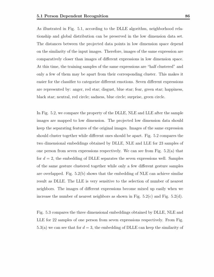
5.1 Person Dependent Recognition 86
As illustrated in Fig. 5.1, according to the DLLE algorithm, neighborhood rela-
tionship and global distribution can be preserved in the low dimension data set.
The distances between the projected data points in low dimension space depend
on the similarity of the input images. Therefore, images of the same expression are
comparatively closer than images of different expressions in low dimension space.
At this time, the training samples of the same expressions are “half clustered” and
only a few of them may be apart from their corresponding cluster. This makes it
easier for the classifier to categorize different emotions. Seven different expressions
are represented by: anger, red star; disgust, blue star; fear, green star; happiness,
black star; neutral, red circle; sadness, blue circle; surprise, green circle.
In Fig. 5.2, we compare the property of the DLLE, NLE and LLE after the sample
images are mapped to low dimension. The projected low dimension data should
keep the separating features of the original images. Images of the same expression
should cluster together while different ones should be apart. Fig. 5.2 compares the
two dimensional embeddings obtained by DLLE, NLE and LLE for 23 samples of
one person from seven expressions respectively. We can see from Fig. 5.2(a) that
for d = 2, the embedding of DLLE separates the seven expressions well. Samples
of the same gesture clustered together while only a few different gesture samples
are overlapped. Fig. 5.2(b) shows that the embedding of NLE can achieve similar
result as DLLE. The LLE is very sensitive to the selection of number of nearest
neighbors. The images of different expressions become mixed up easily when we
increase the number of nearest neighbors as shown in Fig. 5.2(c) and Fig. 5.2(d).
Fig. 5.3 compares the three dimensional embeddings obtained by DLLE, NLE and
LLE for 22 samples of one person from seven expressions respectively. From Fig.
5.3(a) we can see that for d = 3, the embedding of DLLE can keep the similarity of
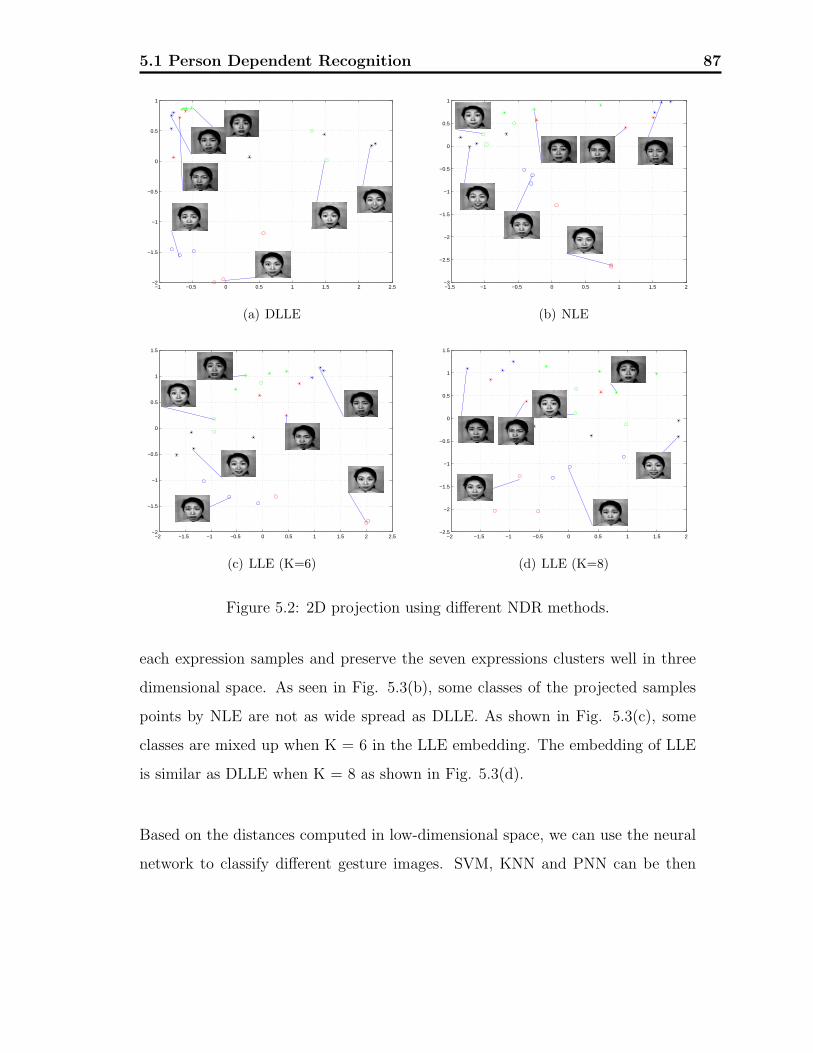
5.1 Person Dependent Recognition 87
−1 −0.5 0 0.5 1 1.5 2 2.5−2
−1.5
−1
−0.5
0
0.5
1
(a) DLLE
−1.5 −1 −0.5 0 0.5 1 1.5 2−3
−2.5
−2
−1.5
−1
−0.5
0
0.5
1
(b) NLE
−2 −1.5 −1 −0.5 0 0.5 1 1.5 2 2.5−2
−1.5
−1
−0.5
0
0.5
1
1.5
(c) LLE (K=6)
−2 −1.5 −1 −0.5 0 0.5 1 1.5 2−2.5
−2
−1.5
−1
−0.5
0
0.5
1
1.5
(d) LLE (K=8)
Figure 5.2: 2D projection using different NDR methods.
each expression samples and preserve the seven expressions clusters well in three
dimensional space. As seen in Fig. 5.3(b), some classes of the projected samples
points by NLE are not as wide spread as DLLE. As shown in Fig. 5.3(c), some
classes are mixed up when K = 6 in the LLE embedding. The embedding of LLE
is similar as DLLE when K = 8 as shown in Fig. 5.3(d).
Based on the distances computed in low-dimensional space, we can use the neural
network to classify different gesture images. SVM, KNN and PNN can be then
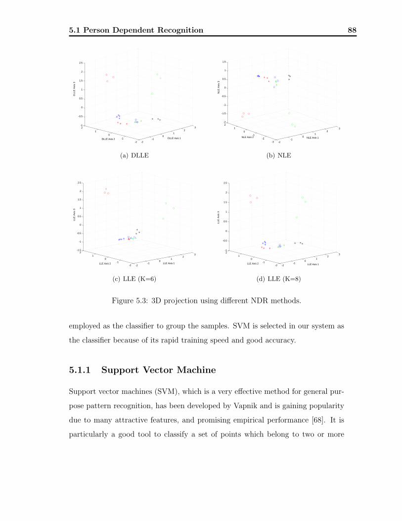
5.1 Person Dependent Recognition 88
-2-1
01
23
-2-1
01
2-1
-0.5
0
0.5
1
1.5
2
2.5
DLLE Axis 1
DLLE
Axi
s 3
DLLE Axis 2
(a) DLLE
-2-1
01
23
-3-2
-10
12
-2
-1.5
-1
-0.5
0
0.5
1
1.5
NLE Axis 1NLE Axis 2
NLE
Axi
s 3
(b) NLE
-2-1
01
23
-2-1
01
2-1.5
-1
-0.5
0
0.5
1
1.5
2
2.5
LLE Axis 2 LLE Axis 1
LLE
Axi
s 3
(c) LLE (K=6)
-2-1
01
23
-2-1
01
2-1
-0.5
0
0.5
1
1.5
2
2.5
LLE Axis 1LLE Axis 2
LLE
Axi
s 3
(d) LLE (K=8)
Figure 5.3: 3D projection using different NDR methods.
employed as the classifier to group the samples. SVM is selected in our system as
the classifier because of its rapid training speed and good accuracy.
5.1.1 Support Vector Machine
Support vector machines (SVM), which is a very effective method for general pur-
pose pattern recognition, has been developed by Vapnik and is gaining popularity
due to many attractive features, and promising empirical performance [68]. It is
particularly a good tool to classify a set of points which belong to two or more
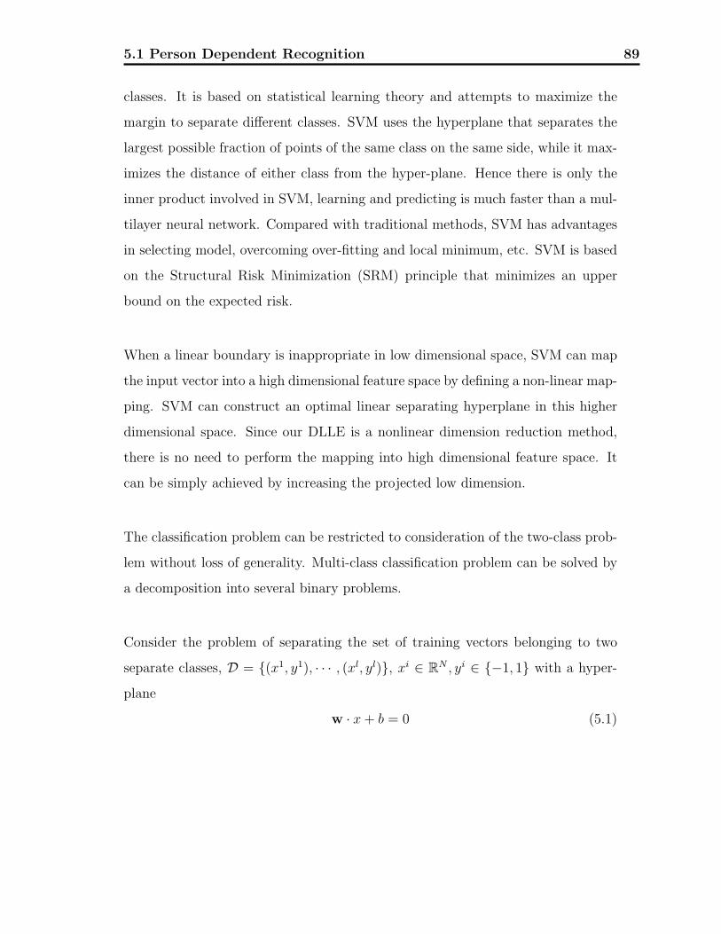
5.1 Person Dependent Recognition 89
classes. It is based on statistical learning theory and attempts to maximize the
margin to separate different classes. SVM uses the hyperplane that separates the
largest possible fraction of points of the same class on the same side, while it max-
imizes the distance of either class from the hyper-plane. Hence there is only the
inner product involved in SVM, learning and predicting is much faster than a mul-
tilayer neural network. Compared with traditional methods, SVM has advantages
in selecting model, overcoming over-fitting and local minimum, etc. SVM is based
on the Structural Risk Minimization (SRM) principle that minimizes an upper
bound on the expected risk.
When a linear boundary is inappropriate in low dimensional space, SVM can map
the input vector into a high dimensional feature space by defining a non-linear map-
ping. SVM can construct an optimal linear separating hyperplane in this higher
dimensional space. Since our DLLE is a nonlinear dimension reduction method,
there is no need to perform the mapping into high dimensional feature space. It
can be simply achieved by increasing the projected low dimension.
The classification problem can be restricted to consideration of the two-class prob-
lem without loss of generality. Multi-class classification problem can be solved by
a decomposition into several binary problems.
Consider the problem of separating the set of training vectors belonging to two
separate classes, D = {(x1, y1), · · · , (xl, yl)}, xi ∈ RN , yi ∈ {−1, 1} with a hyper-
plane
w · x + b = 0 (5.1)
5.1 Person Dependent Recognition 90
which satisfies the following constraints,⎧⎪⎨⎪⎩
w · xi + b ≥ 1, yi = 1
w · xi + b ≤ 1, yi = −1
(5.2)
These constraints can be combined into one set of inequalities:
yi(w · xi + b) ≥ 1, i = 1, 2, · · · , l. (5.3)
The distance d(w, b; xj) of a point xj from the hyperplane (w, b) is,
d(w, b; xj) =|w · xj + b|‖w‖ (5.4)
The optimal hyperplane separating the data is given by maximizing the margin,
ρ, subject to the constraints of equation (5.3). That is minimizing the reciprocal
of the margin. The margin is given by,
ρ(w, b) =2
‖w‖ (5.5)
The problem now is a quadratic programming optimization problem.
min1
2‖w‖2
s.t. yi(w · xi + b) ≥ 1, i = 1, 2, · · · , l. (5.6)
If there exists no hyperplane that can split the ”yes” and ”no” examples, the
Soft Margin method will choose a hyperplane that splits the examples as clean as
possible, while still maximizing the distance to the nearest cleanly split examples.
This method introduces non-negative slack variables and the equation (5.6) now
transforms to
min1
2‖w‖2 + C
l∑i=1
ξi
s.t. yi(w · xi + b) ≥ 1− ξi, ξi ≥ 0, i = 1, 2, · · · , l. (5.7)
5.1 Person Dependent Recognition 91
where C is a penalty parameter. This quadratic programming optimization can be
solved using Lagrange multipliers.
Figure 5.4: Optimal separating hyperplane.
The set of vectors is said to be optimally separated by the hyperplane if it is sepa-
rated without error and the distance between the closest vector to the hyperplane
is maximal.
The multi-class classification problem can be solved by a decomposition where the
multi-class problem is decomposed into several binary problems. Several binary
classifiers have to be constructed or a larger optimization problem is needed. It is
computationally more expensive to solve a multi-class problem than a binary prob-
lem with the same number of samples. Vapnik proposed a one-against-rest (1-a-r)
algorithm [68]. The basic idea for the formulation to solve multi-class SVM prob-
lem can be expressed differently: the problem can be written as “class A against
the rest, class B against the rest, and . . . ”. It is equivalent for each class that “class
n against the rest” for the N binary classification problem. The reduction to binary
problems can be interpreted geometrically as searching N separating hyperplanes.
5.1 Person Dependent Recognition 92
The ith SVM is trained with all of the examples in the ith class with positive
labels while all other examples with negative labels. Given N training data
(x1, y1), (x2, y2), . . . , (xN , yN), where xi ∈ Rn, i = 1, 2, . . . , N and yi ∈ 1, 2, . . . , k is
the class of xi, the ith SVM solves the following problem:
minwi,bi,ξi
1
2‖w‖2 + C
l∑i=1
ξji
s.t. yi(w · xi + bi) ≥ 1− ξji , if yi = j (5.8)
yi(w · xi + bi) ≤ −1 + ξji , if yi �= j
ξji ≥ 0, i = 1, 2, · · · , l.
When the data set is not separable, the penalty term C∑l
i=1 ξji is used to reduce
the training errors. As the solution of equation (5.8), there will be k decision
functions listed below:
y1(w·x1 + b1)
... (5.9)
yk(w·xk + bk)
If class i has the largest value computed by the following decision function with x,
x is classified into class i.
class of x = arg maxi=1,2,...,k
yi(w · xi + bi) (5.10)
The dual problem of equation (5.8) can be solved when the variables are the same
as the number of data. A more detailed description of SVM can be found at [69].
Therefore, after the SVM is conducted, the data set can be classified into several
classes. As shown in the experiments, the SVMs can be effectively utilized for
facial expression recognition.
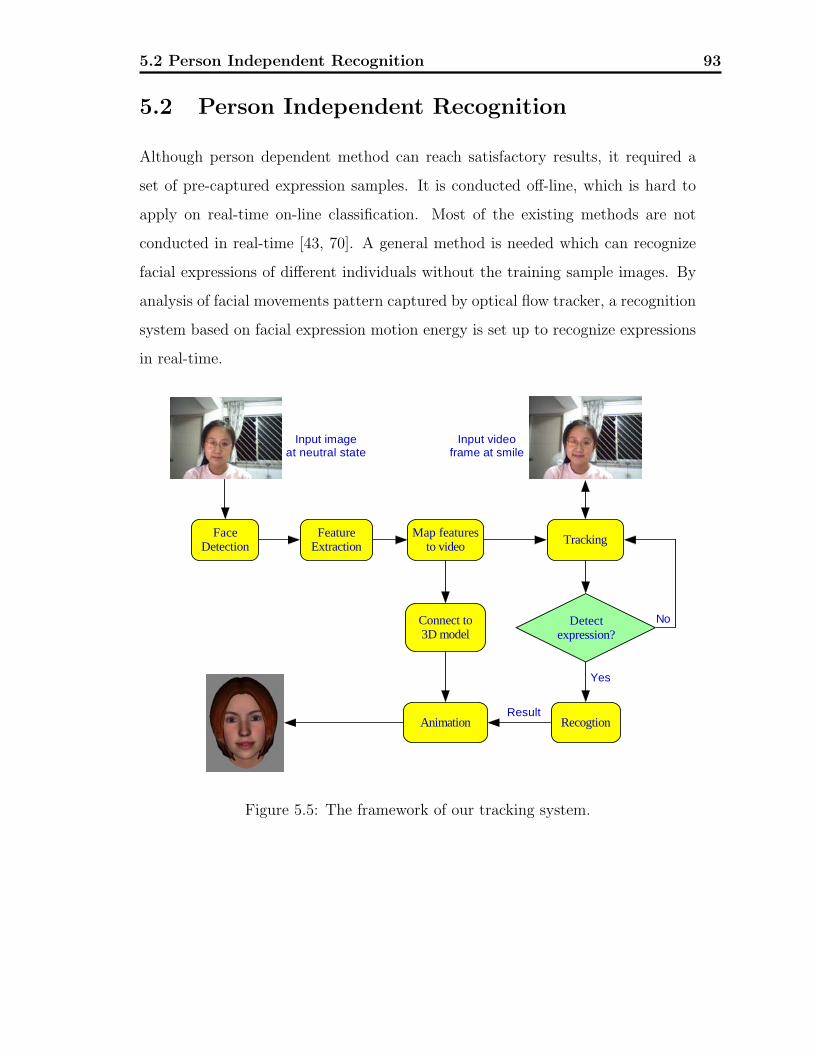
5.2 Person Independent Recognition 93
5.2 Person Independent Recognition
Although person dependent method can reach satisfactory results, it required a
set of pre-captured expression samples. It is conducted off-line, which is hard to
apply on real-time on-line classification. Most of the existing methods are not
conducted in real-time [43, 70]. A general method is needed which can recognize
facial expressions of different individuals without the training sample images. By
analysis of facial movements pattern captured by optical flow tracker, a recognition
system based on facial expression motion energy is set up to recognize expressions
in real-time.
FaceDetection
FeatureExtraction
Map featuresto video
Tracking
Connect to3D model
Animation Recogtion
Detectexpression?
Yes
No
Result
Input imageat neutral state
Input videoframe at smile
Figure 5.5: The framework of our tracking system.
5.2 Person Independent Recognition 94
5.2.1 System Framework
Fig. 5.5 shows the framework of our recognition system. At the initiation stage,
the face image at neutral state is captured. This image is processed in our system
to do face detection, facial features extraction. After the facial features are de-
tected, they are mapped back to the real-time video. The tester’s face should keep
static during this process. At the same time, the connection with the 3D animation
window is set up. These facial features are tracked by L-K optical flow in real-time.
The captured information is processed frame by frame. Once a facial expression
is detected, either the recognition result or the FAP stream is sent to the anima-
tion part. The 3D virtual avatar will display the recognized expression accordingly.
5.2.2 Optical Flow Tracker
Once a face has been located and the facial features are extracted in the scene by
the face tracker, we adopt the optical flow algorithm to determine the motion of
the face. The face motion information can be used for the purposes of classifica-
tion. Firstly, expressions are inherently dynamic events. Secondly, by using motion
information, the task is simplified as it ignores variations in the texture of different
people’s faces. Hence, the facial motion patterns is independent of person who is
expressing the emotion. At the same time, facial motion alone has already been
shown to be a useful cue in the field of human face recognition. There is a growing
argument that the temporal information is a critical factor in the interpretation
of facial expressions [32]. Essa et al. examined the temporal pattern tracked by
optical flow of different expressions but did not account for temporal aspects of
facial motion in their recognition feature vector [33].
5.2 Person Independent Recognition 95
The optical flow methods attempt to calculate the motion between two adjacent
image frames which are taken at times t and t + δt at every pixel position. The
tracker, based on the Lucas-Kanade tracker [37], is capable of following and recov-
ering any of the 21 facial points lost due to lighting variations, rigid or non-rigid
motion, or (to a certain extent) change of head orientation. Automatic recovery,
which uses the nostrils as a reference, is performed based on some heuristics ex-
ploiting the configuration and visual properties of faces.
As a pixel at location (x, y, z) at time t with intensity I(x, y, z, t) will have moved
by δx, δy, δz after time slide δt between the two frames, a translational model of
motion can be given:
I1(x) = I2(x + δx) (5.11)
Let Δt be a small increment in time. Let t be the time at which the first image is
taken, and at time t + Δt the second image is taken. Then for the first image, we
have I1(x) = I(x(t), t), and for the second image, we have I2(x) = I(x(t+ Δt), t+
Δt). Following image constraint equation, it can be given:
I(x(t), t) = I(x(t) + Δx(t), t + Δt) (5.12)
Note that we have removed the subscripts from the expression and have expressed
it purely in terms of displacements in space and time. Assuming the movement
to be small enough, we can develop the image constraint at I(x(t), t) with Taylor
series to get:
I(x(t) + Δx(t), t + Δt) = I(x(t), t) + Δx∂I
∂x+ Δy
∂I
∂y+ Δt
∂I
∂t+ H.O.T
where H.O.T. means higher order terms, which are small enough to be ignored.
Since we have assumed brightness constancy, the first order Taylor series terms
5.2 Person Independent Recognition 96
must vanish:
Δx∂I
∂x+ Δy
∂I
∂y+ Δt
∂I
∂t= 0 (5.13)
Dividing equation (5.13) by an instant of time Δt, we have
Δx
Δt
∂I
∂x+
Δy
Δt
∂I
∂y+
Δt
Δt
∂I
∂t= 0 (5.14)
which results in:
u∂I
∂x+ v
∂I
∂x+ It = 0 (5.15)
or
(∇I)�u + It = 0 (5.16)
where u = (u, v)� denotes the velocity.
Equation (5.16) is known as the Horn-Schunck (H-S) equation. The H-S equation
holds for every pixel of an image. The two key entities in the H-S equation are the
spatial gradient of the image, and the temporal change in the image. These can
be calculated from the image, and are hence known. From these two vectors, we
want to find the velocity vector which, when dotted with the gradient, is cancelled
out by the temporal derivative. In this sense, the velocity vector “explains” the
temporal difference measured in It in terms of the spatial gradient. Unfortunately
this equation has two unknowns but we have only one equation per pixel. So we
cannot solve the H-S equation uniquely at one pixel.
We will now consider a least squares solution proposed by Lucas and Kanade (1981)
(L-K). They assume a translational model and solve for a single velocity vector u
that approximately satisfies the H-S equation for all the pixels in a small neigh-
borhood N of size N ×N . In this way, we obtain a highly over-constrained system
of equations, where we only have 2 unknowns and N2 equations.
5.2 Person Independent Recognition 97
Let N denote a N × N patch around a pixel pi. For each point pi ∈ N , we can
write:
∇I(pi)�u + It(pi) = 0 (5.17)
Thus we arrive at the over-constrained least squares problem, to find the u that
minimizes Ψ(u):
Ψ(u) =∑pi∈N
[∇I(pi)�u + It(pi)]
2 (5.18)
Due to the presence of noise and other factors (like, hardly ever all points pixels
move with the same velocity), the residual will not in general be zero. The least
squares solution will be the one which minimizes the residual. To solve the over-
determined system of equations we use the least squares method:
A�Au = A�b or (5.19)
u = (A�A)−1A�b (5.20)
where A ∈ RN2×2 and b ∈ R
N2are given by:
A =
⎡⎢⎢⎢⎢⎢⎢⎣
∇I(p1)�
∇I(p2)�
...
∇I(pN2)�
⎤⎥⎥⎥⎥⎥⎥⎦
(5.21)
b =
⎡⎢⎢⎢⎢⎢⎢⎣
It(p1)
It(p2)...
It(pN2)
⎤⎥⎥⎥⎥⎥⎥⎦
(5.22)
This means that the optical flow can be found by calculating the derivatives of the
image in all four dimensions.
One of the characteristics of the Lucas-Kanade algorithm, and that of other lo-
cal optical flow algorithms, is that it does not yield a very high density of flow
5.2 Person Independent Recognition 98
vectors, i.e. the flow information fades out quickly across motion boundaries and
the inner parts of large homogenous areas show little motion. Its advantage is the
comparative robustness in presence of noise.
5.2.3 Recognition Results
Fig. 5.6 shows the facial features points(green spots) traced by optical flow method
during a surprise expression. It is cut from a recorded video and illustrated frame
by frame. It can greatly reduce the computation time to track of the specified
limited number of feature points compared to track the holistic dense flow between
successive image frames. As we can seen from these images, the feature points are
tracked closely frame by frame using the L-K optical flow method. With these
tracked position and velocity parameters, expression motion energy can be com-
puted out and expression patterns can be recognized in real-time.
The results of real-time expression recognition are given in Fig. 5.7. The pictures
are captured while the expression occurs. The recognition results are displayed in
real-time in red at the up-left corner of the window. From these pictures, we can
see that the proposed system can effectively detect the facial expressions.
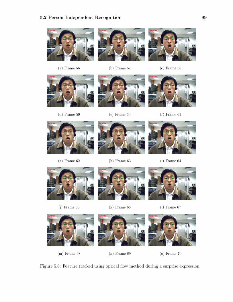
5.2 Person Independent Recognition 99
(a) Frame 56 (b) Frame 57 (c) Frame 58
(d) Frame 59 (e) Frame 60 (f) Frame 61
(g) Frame 62 (h) Frame 63 (i) Frame 64
(j) Frame 65 (k) Frame 66 (l) Frame 67
(m) Frame 68 (n) Frame 69 (o) Frame 70
Figure 5.6: Feature tracked using optical flow method during a surprise expression
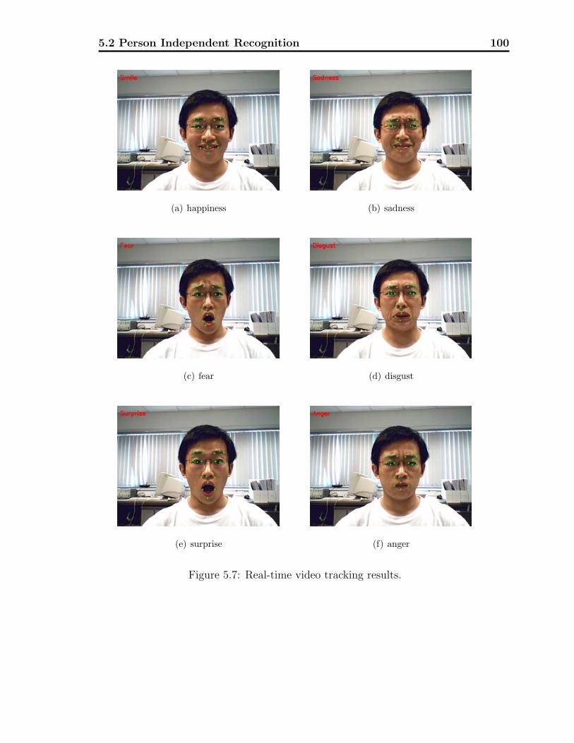
5.2 Person Independent Recognition 100
(a) happiness (b) sadness
(c) fear (d) disgust
(e) surprise (f) anger
Figure 5.7: Real-time video tracking results.
Chapter 63D Facial Expression Animation
In recent years, 3D talking heads have attracted the attention in both research and
industry domains for developing intelligent human computer interaction system.
In our system, a 3D morphable model, Xface, is applied to our face recognition sys-
tem to derive multiple virtual character expressions. It is an open source, platform
independent toolkit, which is developed using C++ programming language incor-
porating object oriented techniques, for developing 3D talking agents. It relies on
MPEG-4 Face Animation (FA) standard. A 3D morphable head model is utilized
to generate multiple facial expressions. When one facial expression occurs, the
movements of tracked feature points are translated to MPEG-4 FAPs. The FAPs
can describe the observed motion in a high level. The virtual model can follow the
human’s expressions naturally. The virtual head also can talk using speech synthe-
sis, another open source tool, Festival [71]. A full-automatic MPEG-4 compliant
facial expression animation and talking pipeline was developed.
101
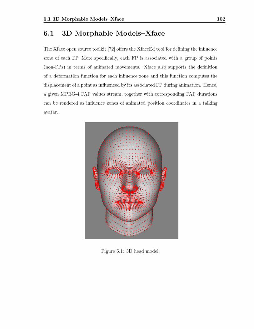
6.1 3D Morphable Models–Xface 102
6.1 3D Morphable Models–Xface
The Xface open source toolkit [72] offers the XfaceEd tool for defining the influence
zone of each FP. More specifically, each FP is associated with a group of points
(non-FPs) in terms of animated movements. Xface also supports the definition
of a deformation function for each influence zone and this function computes the
displacement of a point as influenced by its associated FP during animation. Hence,
a given MPEG-4 FAP values stream, together with corresponding FAP durations
can be rendered as influence zones of animated position coordinates in a talking
avatar.
Figure 6.1: 3D head model.

6.1 3D Morphable Models–Xface 103
6.1.1 3D Avatar Model
We created a 3D avatar model with the image of a young man using the software
3D Studio Max. The avatar model specifies the 3D positional coordinates for an-
imation and rendering, normal coordinates for lighting effects as well as texture
coordinates for texture mapping. Both lighting and texture enhance the appear-
ance of the avatar. The positional coordinates are connected to form a mesh of
triangles that determine the neutral coordinates of the model.
Fig. 6.1 shows the wire frame of the head model. The outlook of the head model
can be changed easily by changing the textures.
6.1.2 Definition of Influence Zone and Deformation Func-
tion
Each FAP corresponds to a set of FP and in turn, each FP corresponds to an
influence zone of non-FP points. We utilize the XfaceEd tool to define influence
zones for each FP in the eyes, eyebrows, and mouth regions. For example, FP
8.4 (Right corner of outer lip contour) is directly affected by FAP 54 (Horizontal
displacement of right outer lip corner) and FAP 60 (Vertical displacement of right
outer lip corner). FP 8.4 is shown as the yellow cross in Fig. 6.2(a) and its influence
zone is shown in terms of big blue dots. Similarly, FP4.1 (left inner eyebrow) is
related to FAP31 (raise left inner eyebrow) and FAP37 (squeeze left inner eyebrow).
FP4.1 is shown as the yellow cross in Fig. 6.2(b) and its influence zone as the group
of big blue dots.
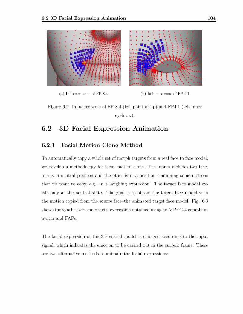
6.2 3D Facial Expression Animation 104
(a) Influence zone of FP 8.4. (b) Influence zone of FP 4.1.
Figure 6.2: Influence zone of FP 8.4 (left point of lip) and FP4.1 (left inner
eyebrow).
6.2 3D Facial Expression Animation
6.2.1 Facial Motion Clone Method
To automatically copy a whole set of morph targets from a real face to face model,
we develop a methodology for facial motion clone. The inputs includes two face,
one is in neutral position and the other is in a position containing some motions
that we want to copy, e.g. in a laughing expression. The target face model ex-
ists only at the neutral state. The goal is to obtain the target face model with
the motion copied from the source face–the animated target face model. Fig. 6.3
shows the synthesized smile facial expression obtained using an MPEG-4 compliant
avatar and FAPs.
The facial expression of the 3D virtual model is changed according to the input
signal, which indicates the emotion to be carried out in the current frame. There
are two alternative methods to animate the facial expressions:
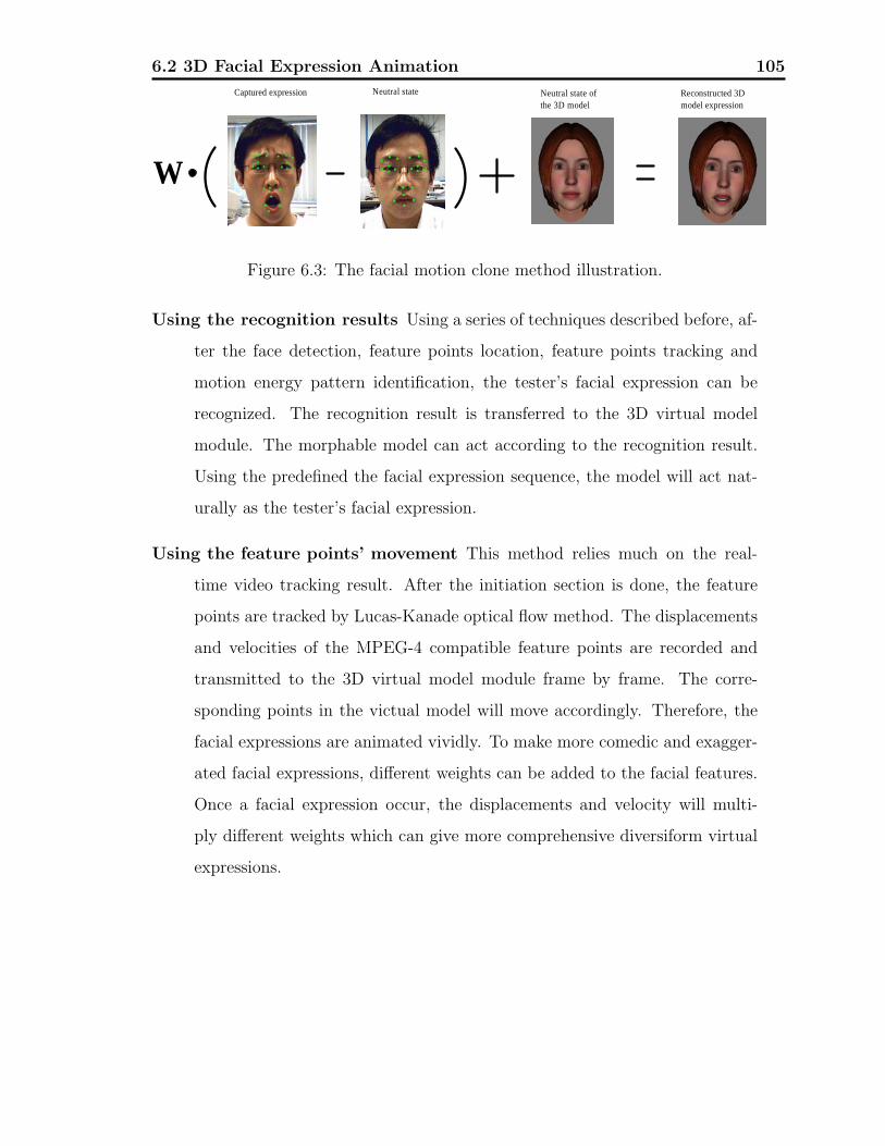
6.2 3D Facial Expression Animation 105
Captured expression Neutral state Neutral state ofthe 3D model
Reconstructed 3Dmodel expression
W
Figure 6.3: The facial motion clone method illustration.
Using the recognition results Using a series of techniques described before, af-
ter the face detection, feature points location, feature points tracking and
motion energy pattern identification, the tester’s facial expression can be
recognized. The recognition result is transferred to the 3D virtual model
module. The morphable model can act according to the recognition result.
Using the predefined the facial expression sequence, the model will act nat-
urally as the tester’s facial expression.
Using the feature points’ movement This method relies much on the real-
time video tracking result. After the initiation section is done, the feature
points are tracked by Lucas-Kanade optical flow method. The displacements
and velocities of the MPEG-4 compatible feature points are recorded and
transmitted to the 3D virtual model module frame by frame. The corre-
sponding points in the victual model will move accordingly. Therefore, the
facial expressions are animated vividly. To make more comedic and exagger-
ated facial expressions, different weights can be added to the facial features.
Once a facial expression occur, the displacements and velocity will multi-
ply different weights which can give more comprehensive diversiform virtual
expressions.

Chapter 7System and Experiments
In this section we present the results of simulation using the proposed static person
dependent and dynamic person independent facial expression recognition methods.
In our system, resolution of the acquired images is 320× 240 pixels. Any captured
images that are in other formats are converted first before further processing. Our
system is developed under Microsoft Visual Studio .NET 2003 using VC++. The
Intel’s Open Source Computer Vision Library (OpenCV) is employed in our system
[73]. The OpenCV Library is developed mainly aimed at real-time computer vision.
It provides a wide variety of tools for image interpretation. The system is executed
on a PC with Pentium IV 2.8G CPU and 512M RAM running Microsoft XP. Our
experiments are carried out under the following assumptions:
• There is only one face contained in one image. The face takes up a significant
area in the image.
• The image resolution should be sufficiently large to facilitate feature extrac-
tion and tracking.
• The user’s face is stationary during the time when the initialization or re-
initialization takes place.
106
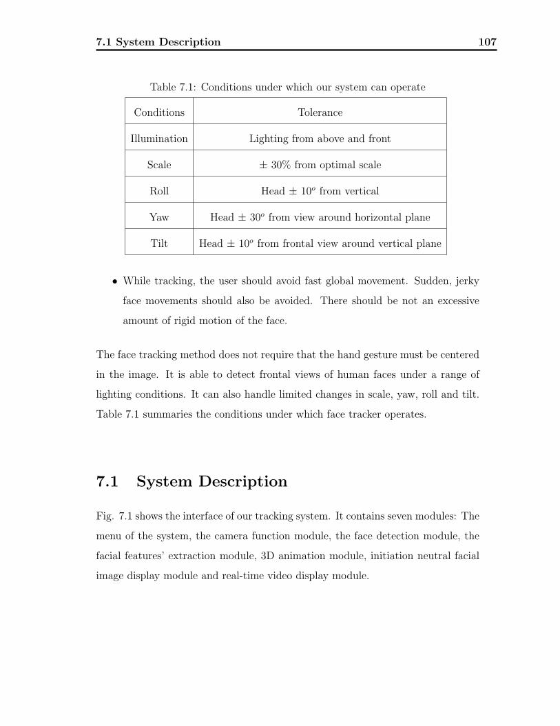
7.1 System Description 107
Table 7.1: Conditions under which our system can operate
Conditions Tolerance
Illumination Lighting from above and front
Scale ± 30% from optimal scale
Roll Head ± 10o from vertical
Yaw Head ± 30o from view around horizontal plane
Tilt Head ± 10o from frontal view around vertical plane
• While tracking, the user should avoid fast global movement. Sudden, jerky
face movements should also be avoided. There should be not an excessive
amount of rigid motion of the face.
The face tracking method does not require that the hand gesture must be centered
in the image. It is able to detect frontal views of human faces under a range of
lighting conditions. It can also handle limited changes in scale, yaw, roll and tilt.
Table 7.1 summaries the conditions under which face tracker operates.
7.1 System Description
Fig. 7.1 shows the interface of our tracking system. It contains seven modules: The
menu of the system, the camera function module, the face detection module, the
facial features’ extraction module, 3D animation module, initiation neutral facial
image display module and real-time video display module.
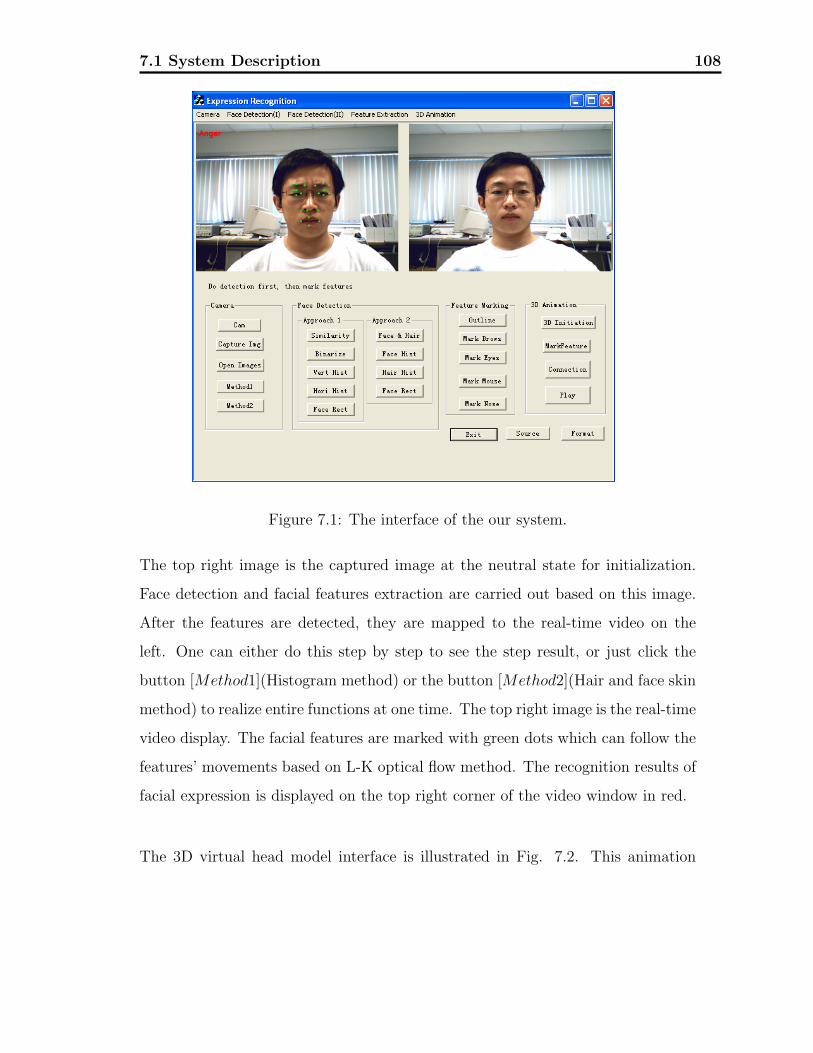
7.1 System Description 108
Figure 7.1: The interface of the our system.
The top right image is the captured image at the neutral state for initialization.
Face detection and facial features extraction are carried out based on this image.
After the features are detected, they are mapped to the real-time video on the
left. One can either do this step by step to see the step result, or just click the
button [Method1](Histogram method) or the button [Method2](Hair and face skin
method) to realize entire functions at one time. The top right image is the real-time
video display. The facial features are marked with green dots which can follow the
features’ movements based on L-K optical flow method. The recognition results of
facial expression is displayed on the top right corner of the video window in red.
The 3D virtual head model interface is illustrated in Fig. 7.2. This animation
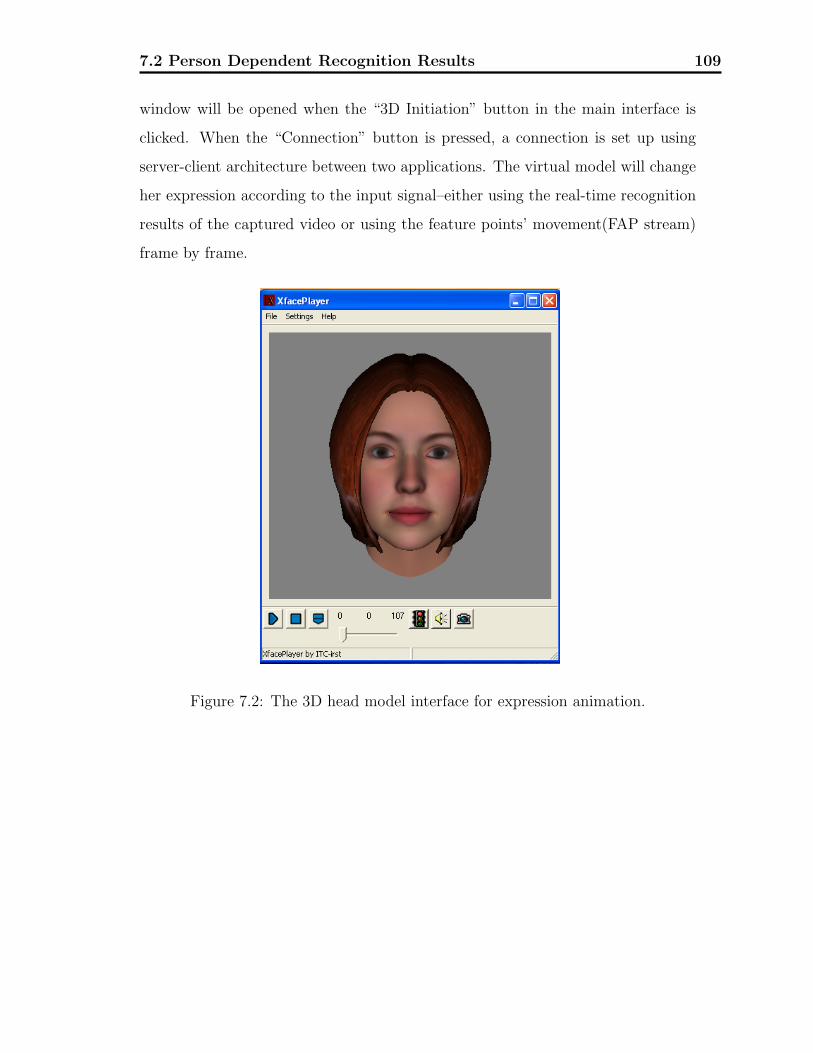
7.2 Person Dependent Recognition Results 109
window will be opened when the “3D Initiation” button in the main interface is
clicked. When the “Connection” button is pressed, a connection is set up using
server-client architecture between two applications. The virtual model will change
her expression according to the input signal–either using the real-time recognition
results of the captured video or using the feature points’ movement(FAP stream)
frame by frame.
Figure 7.2: The 3D head model interface for expression animation.
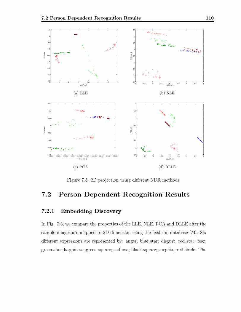
7.2 Person Dependent Recognition Results 110
-1.5 -1 -0.5 0 0.5 1 1.5 2-2.5
-2
-1.5
-1
-0.5
0
0.5
1
1.5
LLE Axis 1
LLE
Axi
s 2
(a) LLE
-2 -1.5 -1 -0.5 0 0.5 1 1.5 2-2.5
-2
-1.5
-1
-0.5
0
0.5
1
1.5
NLE Axis 1
NLE
Axi
s 2
(b) NLE
0.0904 0.0906 0.0908 0.091 0.0912 0.0914 0.0916 0.0918 0.092 0.0922-0.2
-0.15
-0.1
-0.05
0
0.05
0.1
0.15
PCA Axis 1
PC
A A
xis
2
(c) PCA
-2 -1.5 -1 -0.5 0 0.5 1 1.5 2-1.5
-1
-0.5
0
0.5
1
1.5
2
DLLE Axis 1
DLL
E A
xis
2
(d) DLLE
Figure 7.3: 2D projection using different NDR methods.
7.2 Person Dependent Recognition Results
7.2.1 Embedding Discovery
In Fig. 7.3, we compare the properties of the LLE, NLE, PCA and DLLE after the
sample images are mapped to 2D dimension using the feedtum database [74]. Six
different expressions are represented by: anger, blue star; disgust, red star; fear,
green star; happiness, green square; sadness, black square; surprise, red circle. The

7.2 Person Dependent Recognition Results 111
projected low dimension data should keep the separating features of the original im-
ages. Images of the same expression should cluster together while different should
be apart. There are 120 samples of one person from six expressions respectively (20
samples per expression). These samples are manually selected after the automatic
selection described in chapter 3. We can see from Fig. 7.3(d) that for d = 2, differ-
ent expressions’ embedding of LLE are separated. However, the red and blue points
are overlapped and not separatable in 2D dimension. Fig. 7.3(b) shows the embed-
ding of NLE. It can be seen that in general they are separated, but the boundary
between different groups are not clear. PCA achieves similar result as NLE which
is shown in Fig. 7.3(c). The samples of the same expression are not so centralized
and the red and blue star samples are mixed up. As illustrated in Fig. 7.3(d),
we can see that DLLE can separate the six expressions well. Samples of the same
expression cluster together while different expression samples are clearly separated.
Fig. 7.4 shows 3D embeddings obtained by LLE, NLE, PCA and DLLE. As illus-
trated in the four images, DLLE can give a better separated embedding compared
to other methods-same expressions are more centralized while different expressions
separated apart. Different expressions can be easily separated by linear separator.
As illustrated in Fig. 7.4(a) and Fig. 7.4(c), LLE and PCA both have some over-
laps.
The reason is that LLE is an unsupervised learning algorithm. It selects the near-
est neighbors to reconstruct the manifold in the low dimensional space. There are
two types of variations in the data set: the different kinds of facial expressions
and the varying intensity for every kind of facial expression. Generally, LLE can
catch the second type of variation-an image sequence is mapped in a “line”, and
LLE can keep the sequences with different expressions distinctive when there is
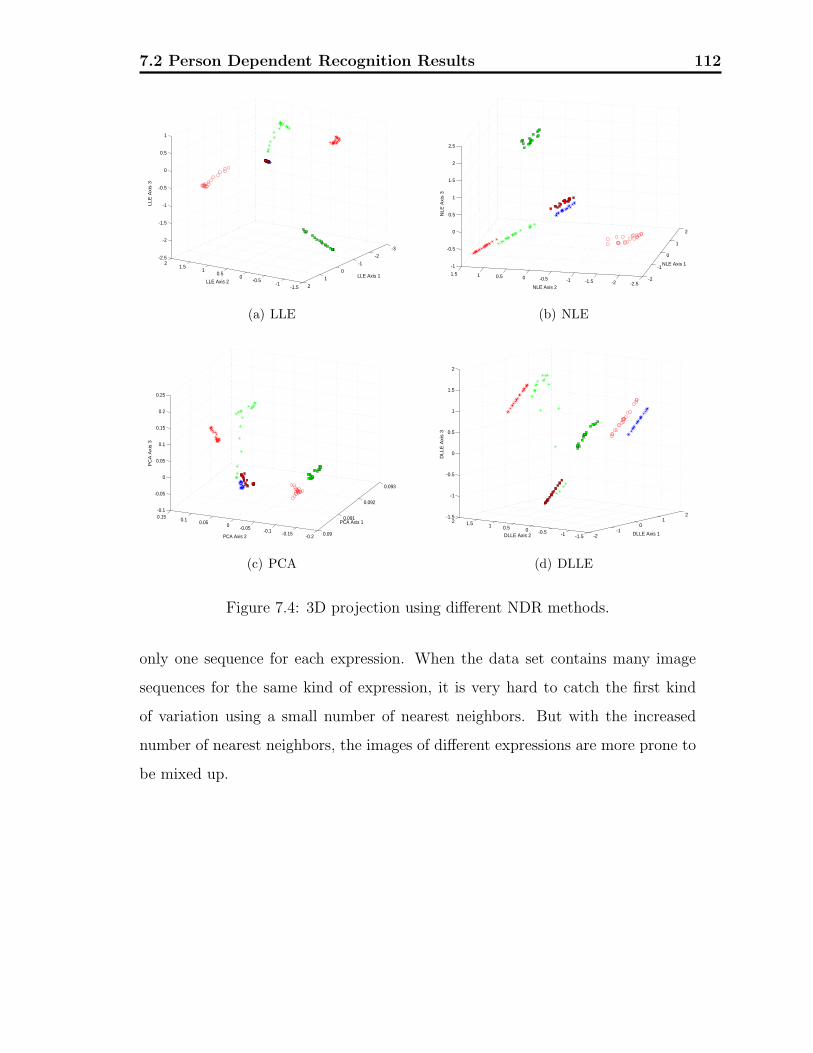
7.2 Person Dependent Recognition Results 112
-1.5-1
-0.50
0.51
1.52
-3-2
-1
0
1
2
-2.5
-2
-1.5
-1
-0.5
0
0.5
1
LLE Axis 2LLE Axis 1
LLE
Axi
s 3
(a) LLE
-2
-1
0
1
2
-2.5-2-1.5-1-0.500.511.5
-1
-0.5
0
0.5
1
1.5
2
2.5
NLE Axis 2
NLE Axis 1
NLE
Axi
s 3
(b) NLE
0.09
0.091
0.092
0.093
-0.2-0.15-0.1-0.0500.050.10.15-0.1
-0.05
0
0.05
0.1
0.15
0.2
0.25
PC
A A
xis
3
PCA Axis 1
PCA Axis 2
(c) PCA
-2-1
01
2
-1.5-1-0.500.511.52-1.5
-1
-0.5
0
0.5
1
1.5
2
DLLE Axis 1DLLE Axis 2
DLLE
Axi
s 3
(d) DLLE
Figure 7.4: 3D projection using different NDR methods.
only one sequence for each expression. When the data set contains many image
sequences for the same kind of expression, it is very hard to catch the first kind
of variation using a small number of nearest neighbors. But with the increased
number of nearest neighbors, the images of different expressions are more prone to
be mixed up.
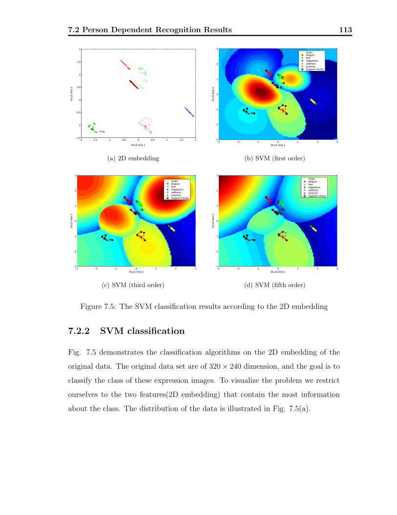
7.2 Person Dependent Recognition Results 113
-2 -1.5 -1 -0.5 0 0.5 1 1.5 2-1.5
-1
-0.5
0
0.5
1
1.5
2
DLLE Axis 1
DLL
E A
xis
2
(a) 2D embedding
-3 -2 -1 0 1 2 3-3
-2
-1
0
1
2
3
DLLE Axis 1
DLL
E A
xis
2
angerdisgustfearhappinesssadnesssurpriseSupport Vector
(b) SVM (first order)
-3 -2 -1 0 1 2 3-3
-2
-1
0
1
2
3
DLLE Axis 1
DLL
E A
xis
2
angerdisgustfearhappinesssadnesssurpriseSupport Vector
(c) SVM (third order)
-3 -2 -1 0 1 2 3-3
-2
-1
0
1
2
3
DLLE Axis 1
DLL
E A
xis
2
angerdisgustfearhappinesssadnesssurpriseSupport Vector
(d) SVM (fifth order)
Figure 7.5: The SVM classification results according to the 2D embedding
7.2.2 SVM classification
Fig. 7.5 demonstrates the classification algorithms on the 2D embedding of the
original data. The original data set are of 320× 240 dimension, and the goal is to
classify the class of these expression images. To visualize the problem we restrict
ourselves to the two features(2D embedding) that contain the most information
about the class. The distribution of the data is illustrated in Fig. 7.5(a).
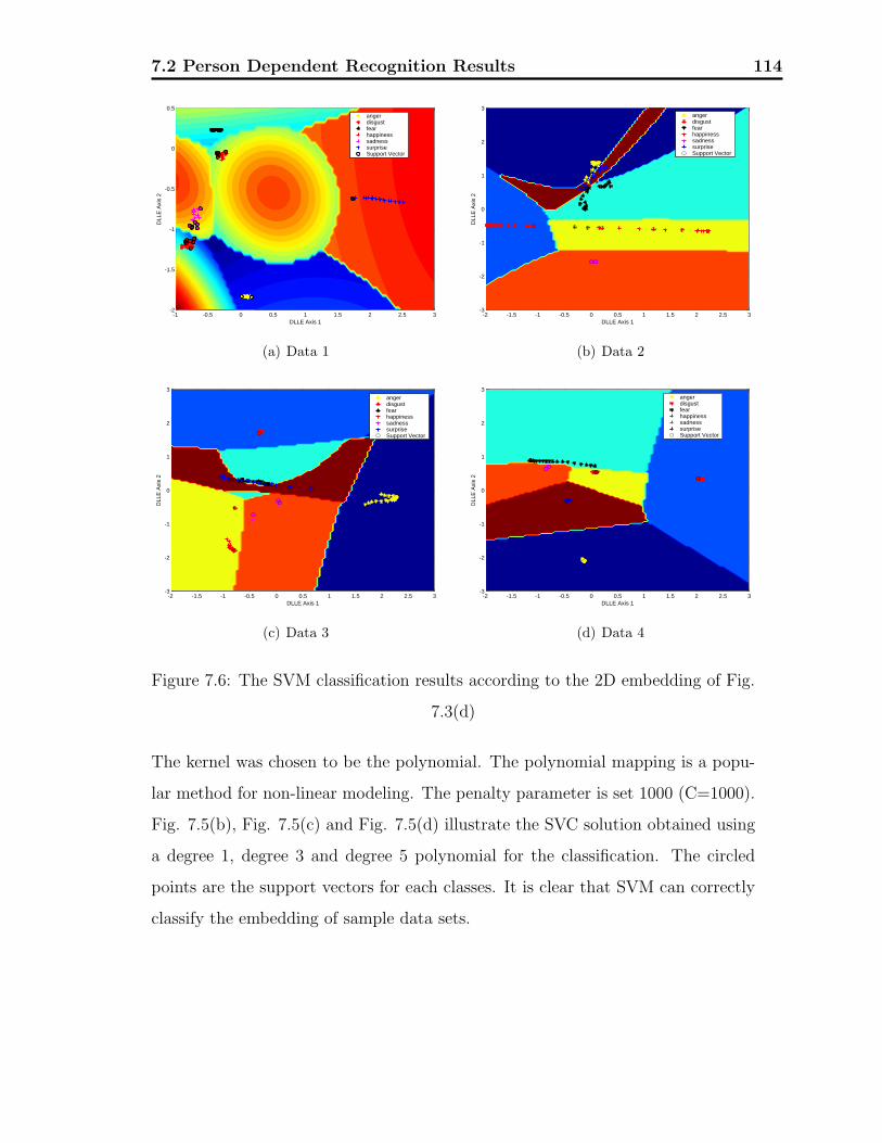
7.2 Person Dependent Recognition Results 114
-1 -0.5 0 0.5 1 1.5 2 2.5 3-2
-1.5
-1
-0.5
0
0.5
DLLE Axis 1
DLL
E A
xis
2
angerdisgustfearhappinesssadnesssurpriseSupport Vector
(a) Data 1
-2 -1.5 -1 -0.5 0 0.5 1 1.5 2 2.5 3-3
-2
-1
0
1
2
3
DLLE Axis 1
DLL
E A
xis
2
angerdisgustfearhappinesssadnesssurpriseSupport Vector
(b) Data 2
-2 -1.5 -1 -0.5 0 0.5 1 1.5 2 2.5 3-3
-2
-1
0
1
2
3
DLLE Axis 1
DLL
E A
xis
2
angerdisgustfearhappinesssadnesssurpriseSupport Vector
(c) Data 3
-2 -1.5 -1 -0.5 0 0.5 1 1.5 2 2.5 3-3
-2
-1
0
1
2
3
DLLE Axis 1
DLL
E A
xis
2
angerdisgustfearhappinesssadnesssurpriseSupport Vector
(d) Data 4
Figure 7.6: The SVM classification results according to the 2D embedding of Fig.
7.3(d)
The kernel was chosen to be the polynomial. The polynomial mapping is a popu-
lar method for non-linear modeling. The penalty parameter is set 1000 (C=1000).
Fig. 7.5(b), Fig. 7.5(c) and Fig. 7.5(d) illustrate the SVC solution obtained using
a degree 1, degree 3 and degree 5 polynomial for the classification. The circled
points are the support vectors for each classes. It is clear that SVM can correctly
classify the embedding of sample data sets.
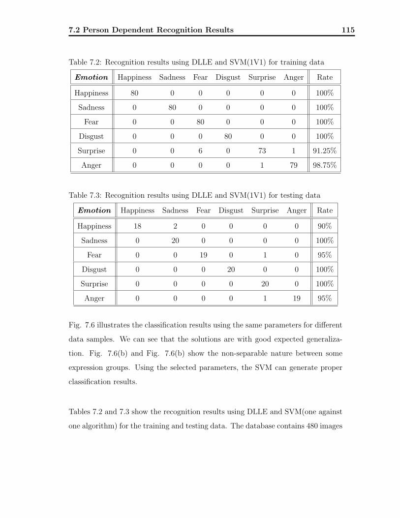
7.2 Person Dependent Recognition Results 115
Table 7.2: Recognition results using DLLE and SVM(1V1) for training data
Emotion Happiness Sadness Fear Disgust Surprise Anger Rate
Happiness 80 0 0 0 0 0 100%
Sadness 0 80 0 0 0 0 100%
Fear 0 0 80 0 0 0 100%
Disgust 0 0 0 80 0 0 100%
Surprise 0 0 6 0 73 1 91.25%
Anger 0 0 0 0 1 79 98.75%
Table 7.3: Recognition results using DLLE and SVM(1V1) for testing data
Emotion Happiness Sadness Fear Disgust Surprise Anger Rate
Happiness 18 2 0 0 0 0 90%
Sadness 0 20 0 0 0 0 100%
Fear 0 0 19 0 1 0 95%
Disgust 0 0 0 20 0 0 100%
Surprise 0 0 0 0 20 0 100%
Anger 0 0 0 0 1 19 95%
Fig. 7.6 illustrates the classification results using the same parameters for different
data samples. We can see that the solutions are with good expected generaliza-
tion. Fig. 7.6(b) and Fig. 7.6(b) show the non-separable nature between some
expression groups. Using the selected parameters, the SVM can generate proper
classification results.
Tables 7.2 and 7.3 show the recognition results using DLLE and SVM(one against
one algorithm) for the training and testing data. The database contains 480 images
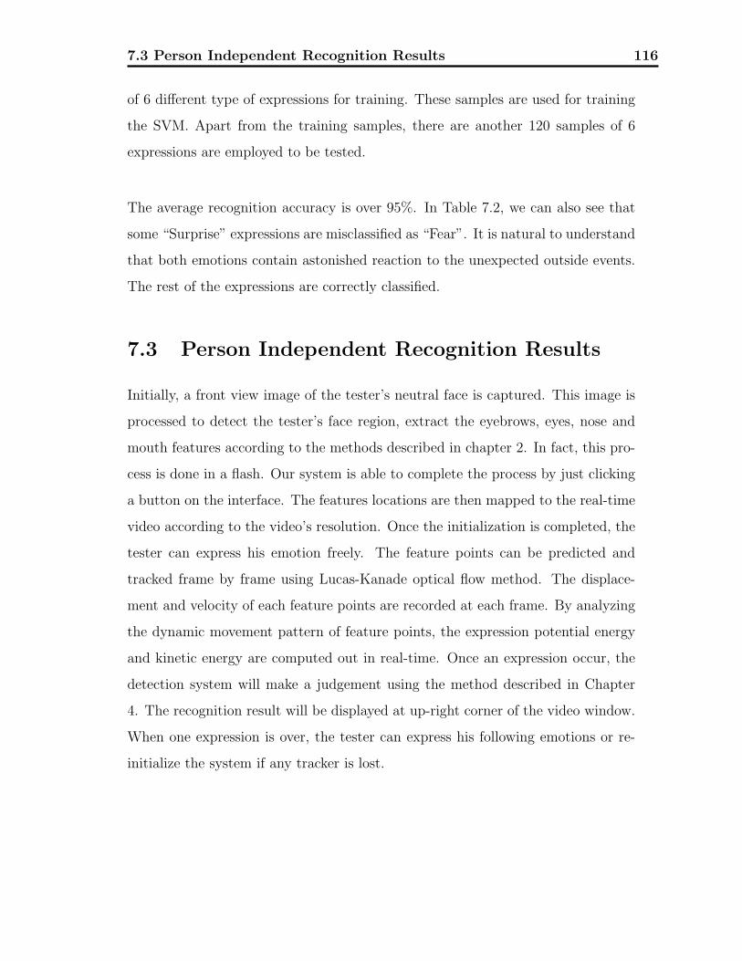
7.3 Person Independent Recognition Results 116
of 6 different type of expressions for training. These samples are used for training
the SVM. Apart from the training samples, there are another 120 samples of 6
expressions are employed to be tested.
The average recognition accuracy is over 95%. In Table 7.2, we can also see that
some “Surprise” expressions are misclassified as “Fear”. It is natural to understand
that both emotions contain astonished reaction to the unexpected outside events.
The rest of the expressions are correctly classified.
7.3 Person Independent Recognition Results
Initially, a front view image of the tester’s neutral face is captured. This image is
processed to detect the tester’s face region, extract the eyebrows, eyes, nose and
mouth features according to the methods described in chapter 2. In fact, this pro-
cess is done in a flash. Our system is able to complete the process by just clicking
a button on the interface. The features locations are then mapped to the real-time
video according to the video’s resolution. Once the initialization is completed, the
tester can express his emotion freely. The feature points can be predicted and
tracked frame by frame using Lucas-Kanade optical flow method. The displace-
ment and velocity of each feature points are recorded at each frame. By analyzing
the dynamic movement pattern of feature points, the expression potential energy
and kinetic energy are computed out in real-time. Once an expression occur, the
detection system will make a judgement using the method described in Chapter
4. The recognition result will be displayed at up-right corner of the video window.
When one expression is over, the tester can express his following emotions or re-
initialize the system if any tracker is lost.
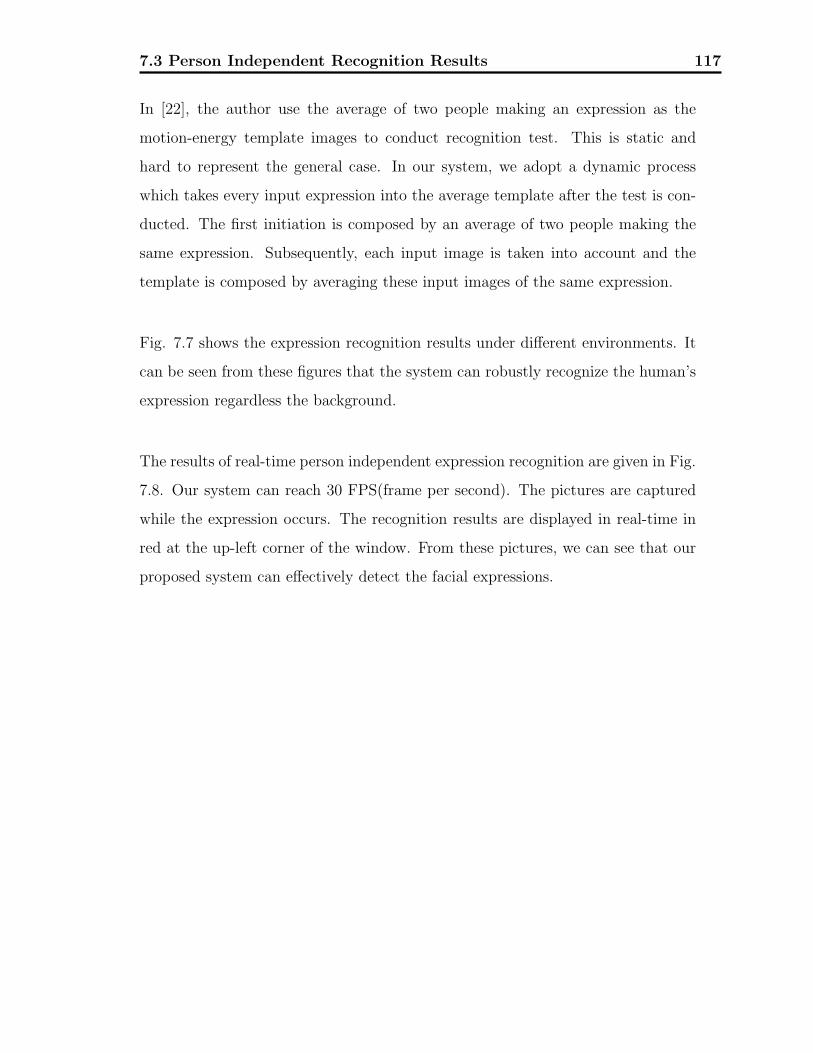
7.3 Person Independent Recognition Results 117
In [22], the author use the average of two people making an expression as the
motion-energy template images to conduct recognition test. This is static and
hard to represent the general case. In our system, we adopt a dynamic process
which takes every input expression into the average template after the test is con-
ducted. The first initiation is composed by an average of two people making the
same expression. Subsequently, each input image is taken into account and the
template is composed by averaging these input images of the same expression.
Fig. 7.7 shows the expression recognition results under different environments. It
can be seen from these figures that the system can robustly recognize the human’s
expression regardless the background.
The results of real-time person independent expression recognition are given in Fig.
7.8. Our system can reach 30 FPS(frame per second). The pictures are captured
while the expression occurs. The recognition results are displayed in real-time in
red at the up-left corner of the window. From these pictures, we can see that our
proposed system can effectively detect the facial expressions.
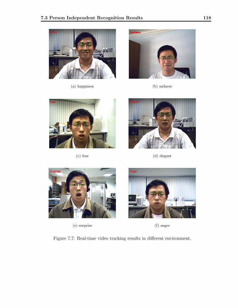
7.3 Person Independent Recognition Results 118
(a) happiness (b) sadness
(c) fear (d) disgust
(e) surprise (f) anger
Figure 7.7: Real-time video tracking results in different environment.
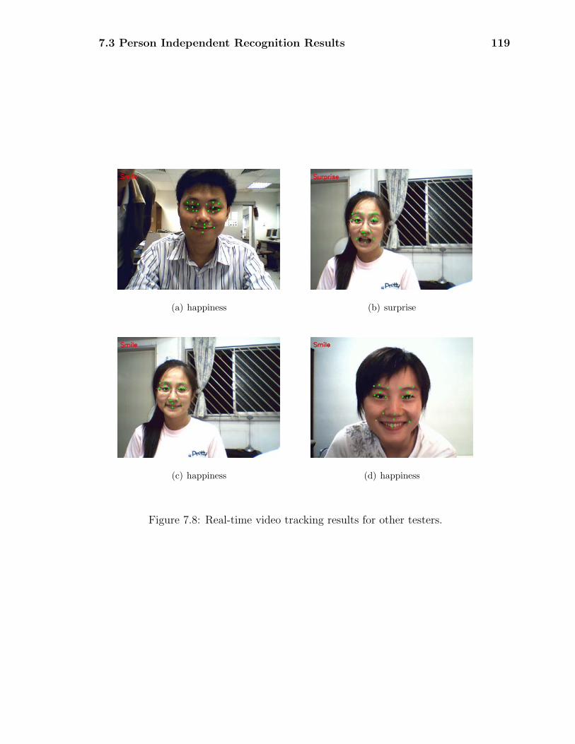
7.3 Person Independent Recognition Results 119
(a) happiness (b) surprise
(c) happiness (d) happiness
Figure 7.8: Real-time video tracking results for other testers.
Chapter 8Conclusion
8.1 Summary
This thesis attempts to recognize the six emotions universally associated with
unique facial expressions. Vision based capturing of expression has been a chal-
lenging problem due to the high degree of freedom of facial motions. In our work,
two methods for person-dependent and person-independent recognition are pre-
sented. Our methods can successfully recognize the static, off-line captured facial
expression images, track and identify dynamic on-line facial expressions of real-time
video from one web camera. The face area is automatically detected and located
by making using of face detection and skin hair color information. Our system
utilizes a subset of Feature Points (FPs) for describing the facial expressions which
is supported by the MPEG-4 standard. 21 facial features are extracted from the
captured video and tracked by optical flow algorithm.
In this thesis, an unsupervised learning algorithm, DLLE, has been developed
to discover the intrinsic structure of the data. These discovered properties are
used to compute their corresponding low-dimensional embedding. It is conducted
120

8.2 Future Research 121
by estimating the probability density function from the input data and using an
exponential neighbor finding method to automatically obtain the embedding. As-
sociated with SVM, a high recognition accuracy algorithm has been developed for
static facial expression recognition. We also give out the test results by DLLE,
NLE and LLE embedding from where we can see that our method is better in
separating the high-dimensional data in low-dimensional space.
We also incorporate facial expression motion energy to describe the facial muscle’s
tension during the expressions for person-independent tracking. It is composed by
the expression potential energy and kinetic energy. The potential energy is used
as the description of the facial muscle’s tension during the expression. Kinetic
energy is the energy which a feature point possesses as a result of facial motion.
For each facial expression pattern, the energy pattern is unique and it is utilized
for the further classification. Combined with the rule based method, the recogni-
tion accuracy can be improved for real-time person-independent facial expression
recognition.
A 3D realistic interactive expression model is integrated into our face recognition
and tracking system which can derive multiple virtual character expressions ac-
cording to the input expression in real-time.
8.2 Future Research
There are a number of directions which could be done for future work.
• One limitation of the current system is that it can detects only one front view
face looking at the camera. Multiple face detection and feature extraction
could be further improved. Since the current system can deal with some

8.2 Future Research 122
degree of lighting and orientation variation, the resolution of the image would
be the main problem to concur for multi-person expression analysis.
• One direction to advance our current work is to combine the human speech
and make both virtual and real robotic talking head for human emotion
understanding and intelligent human computer interface, and explore virtual
human companion for learning and information seeking.
Bibliography
[1] C. Darwin, The Expression of the Emotions in Man and Animals. London:
John Murray, Albemarle Street, 1872.
[2] C. Kotropoulos and I. Pitas, “Rule-based face detection in frontal views,” in
Proc. of IEEE Int. Conf. on Acoustics, Speech and Signal Processing (ICASSP
97), vol. IV, pp. 2537–2540, April 1997.
[3] G. Yang and T. S. Huang, “Human face detection in a complex background,”
Pattern Recognition, vol. 27, pp. 53–63, 1994.
[4] M. Pantic and L. J. M. Rothkrantz, “An expert system for recognition of facial
actions and their intensity,” Image and Vision Computing, vol. 18, pp. 881–
905, 2000.
[5] S. A. Sirohey, “Human face segmentation and identification,” Tech. Rep. CS-
TR-3176, 1993.
123
Bibliography 124
[6] H. Graf, T. Chen, E. Petajan, and E. Cosatto, “Locating faces and facial
parts,” in Int. Workshop on Automatic Face and Gesture Recognition, pp. 41–
46, 1995.
[7] K. Sobottka and I. Pitas, “Face localization and facial feature extraction based
on shape and color information,” in Proc. of IEEE Int. Conf. on Image Pro-
cessing, pp. 483–486, 1996.
[8] C. T. T. Cootes, D. Cooper and J. Graham, “Active shape models-their train-
ing and application,” Computer Vision and Image Understanding, vol. 61,
pp. 38–59, 1995.
[9] T. F. Cootes, G. J. Edwards, and C. J. Taylor, “Active appearance models,”
in European Conf. on Computer Vision (ECCV), vol. 2, 1998.
[10] M. Turk and A. Pentland, “Eigenfaces for recognition,” Journal of Cognitive
Neuroscience, vol. 3, no. 1, p. 71C86, 1991.
[11] F. Fogelman Soulie, E. Viennet, and B. Lamy, “Multi-modular neural network
architectures: applications in optical character and human face recognition.,”
IEEE Trans. on Pattern Analysis and Machine Intelligence, vol. 7, p. 721,
1993.
[12] P. Michel and R. E. Kaliouby, “Real time facial expression recognition in video
using support vector machines,” in 5th Int. Conf. on Multimodal interfaces
table of contents, vol. 3, pp. 258 – 264, 2003.
[13] S. Y. Kang, K. H. Young, and R.-H. Park, “Hybrid approaches to frontal
view face recognition using the hidden markov model and neural network.,”
Pattern Recognition, vol. 31, pp. 283–293, Mar. 1998.
Bibliography 125
[14] M. J. Lyons, S. Akamatsu, M. Kamachi, and J. Gyoba, “Coding facial ex-
pressions with gabor wavelets,” in Proc. of the Third IEEE Int. Conf. on
Automatic Face and Gesture Recognition, pp. 200–205, April 1998.
[15] R. Brunelli and T. Poggio, “Face recognition: Features versus templates,”
IEEE Trans. on Pattern Analysis and Machine Intelligence, vol. 15, no. 10,
pp. 1042–1052, 1993.
[16] I. Craw, D. Tock, and A. Bennett, “Finding face features,” in European Conf.
on Computer Vision (ECCV), pp. 92–96, 1992.
[17] K. Waters, “A muscle model for animating three-dimensional facial expres-
sion,” Computer Graphics, vol. 21, July 1987.
[18] K. Scott, D. Kagels, S. Watson, H. Rom, J. Wright, M. Lee, and K. Hussey,
“Synthesis of speaker facial movement to match selected speech sequences,”
in In Proc. 5th Australian Conf. on Speech Science and Technology, 1994.
[19] B. Horn and B. Schunck, “Determining optical flow,” Artificial Intelligence,
vol. 17, no. 1-3, pp. 185 – 203, 1981.
[20] M. N. Dailey and G. W. Cottrell, “PCA gabor for expression recognition,”
Tech. Rep. CS1999-0629, 26, 1999.
[21] M. Bartlett, Face Image Analysis by Unsupervised Learning and Redundancy
Reduction. PhD thesis, University of California, San Diego, 1998.
[22] I. A. Essa and A. Pentland, “Facial expression recognition using a dy-
namic model and motion energy,” in Int. Conf. on Computer Vision (ICCV),
pp. 360–367, 1995.
Bibliography 126
[23] P. Ekman and W. Friesen, Facial Action Coding System: A Technique for the
Measurement of Facial Movement. Palo Alto, California, USA: Consulting
Psychologists Press, 1978.
[24] ISO/IEC IS 14496-2 Visual: A compression codec for visual data. 1999.
[25] A. Young and H. E. Ellis, Handbook of Research on Face Processing. North-
Holland,Amsterdam: Elsevier Science Publishers B.V., 1989.
[26] C. Padgett and G. Cottrell, Representing face images for classifying emotions,
vol. 9. Cambridge, MA: MIT Press, 1997.
[27] C. Padgett, G. Cottrell, and B. Adolps, “Categorical perception in facial emo-
tion classification,” in Proc. Cognitive Science Conf., vol. 18, pp. 249–253,
1996.
[28] Y. Yacoob and L. Davis, “Recognizing human facial expressions from long
image sequences using optical flow,” IEEE Trans. on Pattern Analysis and
Machine Intelligence, vol. 18, pp. 636–642, June 1996.
[29] T. Otsuka and J. Ohya, “Recognition of facial expressions using HMM with
continuous output probabilities,” in Proc. 5th IEEE Int. Workshop on Robot
and Human Communication RO-MAN, pp. 323–328, 1996.
[30] Y.-L. Tian, T. Kanade, and J. Cohn, “Recognizing action units for facial
expression analysis,” IEEE Trans. on Pattern Analysis and Machine Intelli-
gence, vol. 23, pp. 97 – 115, February 2001.
[31] M. Pantic and J. Rothkrantz, “Facial action recognition for facial expres-
sion analysis from static face images,” IEEE Trans. on Systems, Man and
Cybernetics-Part B, vol. 34, June 2004.
Bibliography 127
[32] C. E. Izard, “Facial expressions and the regulation of emotions,” Journal of
Personality and Social Psychology, vol. 58, no. 3, pp. 487–498, 1990.
[33] I. Essa and A. Pentland, “Coding, analysis, interpretation, and recognition
of facial expressions,” IEEE Trans. on Pattern Analysis and Machine Intelli-
gence, vol. 19, no. 7, 1997.
[34] P. Roivainen, H. Li, and R. Forcheimer, “3-D motion estimation in model-
based facial image coding,” IEEE Trans. on Pattern Analysis and Machine
Intelligence, vol. 15, pp. 545–555, 1993.
[35] G. Donato, M. S. Bartlett, J. C. Hager, P. Ekman, and T. J. Sejnowski,
“Classifying facial actions,” IEEE Trans. on Pattern Analysis and Machine
Intelligence, vol. 21, no. 10, pp. 974–989, 1999.
[36] K. Mase, “Recognition of facial expression from optical flow,” Institute of elec-
tronics information and communication engineers Trans., vol. E74, pp. 3474–
3483, 1991.
[37] B. Lucas and T. Kanade, “An iterative image registration technique with an
application to stereo vision,” in Proc. of the 7th Int. Joint Conf. on Artificial
Intelligence (IJCAI ’81), pp. 674–679, April 1981.
[38] J. Lien, Automatic recognition of facial expression using hidden Markov models
and estimation of expression intensity. PhD thesis, The Robotics Institute,
CMU, April 1998.
[39] X. Zhou, X. S. Huang, and Y. S. Wang, “Real-time facial expression recog-
nition in the interactive game based on embedded hidden markov model,” in
Proc. of the Int. Conf. on Computer Graphics, Imaging and Visualization,
pp. 144–148, 2004.
Bibliography 128
[40] P. Ekman and R. J. Davidson, The Nature of Emotion Fundamental Ques-
tions. New York: Oxford Univ. Press, 1994.
[41] M. H. Yang, D. Kriegman, and N. Ahuja, “Detecting faces in images: A
survey,” IEEE Trans. on Pattern Analysis and Machine Intelligence, vol. 24,
pp. 34–58, Jan. 2002.
[42] D. A. Forsyth and J. Ponce, Computer Vision: A Modern Approach. Upper
Saddle River, New Jersey: Prentice Hall, 2002.
[43] M. Pantic and L. J. M. Rothkrantz, “Automatic analysis of facial expres-
sions: The state of the art,” IEEE Trans. on Pattern Analysis and Machine
Intelligence, vol. 22, no. 12, pp. 1424–1445, 2000.
[44] S. McKenna, S. Gong, and Y. Raja, “Modelling facial colour and identity with
gaussian mixtures,” Parttern Recognition, vol. 31, pp. 1883–1892, December
1998.
[45] J. Yang, W. Lu, and A. Waibel, “Skin-color modeling and adaptation,” in
Proc. of Asian Conference on Computer Vision, pp. 687–694, 1998.
[46] J. Yang and A. Waibel, “A real-time face tracker,” in Proc. of the third IEEE
Workshop on Applications of Computer Vision, 1996.
[47] M. Jones and J. Rehg, “Statistical color models with application to skin detec-
tion,” International Journal of Computer Vision, vol. 46, pp. 81–96, January
2002.
[48] C. Harris and M. Stephens, “A combined edge and corner detector,” in Proc.
of the 4th Alvey Vision Conference, pp. 147–151, 1988.
Bibliography 129
[49] D. Williams and M. Shah, “Edge characterization using normalized edge detec-
tor,” Computer Vision, Graphics and Image Processing, vol. 55, pp. 311–318,
July 1993.
[50] K. Hotta, “A robust face detection under partial occlusion,” in Proc. of Int.
Conf. on Image Processing, pp. 597–600, 2004.
[51] N. Tsapatsoulis, A. Raouzaiou, S. Kollias, R. Cowie, and E. Douglas-Cowie,
MPEG-4 Facial Animation, ch. Emotion Recognition and Synthesis based on
MPEG-4 FAPs. John Wiley & Sons, 2002.
[52] J. Bassili, “Emotion recognition: The role of facial movement and the relative
importance of upper and lower areas of the face,” Journal of Personality Social
Psychology, vol. 37, pp. 2049–2059, 1979.
[53] J. Wang, Z. Changshui, and K. Zhongbao, “An analytical mapping for LLE
and its application in multi-pose face synthesis,” in 14th British Machine
Vision Conference, September.
[54] M. Bartlett and T. Sejnowski, “Independent components of face images: A
representation for face recognition,” in Proc. of the 4th Annual Joint Sympo-
sium on Neural Computation, 1997.
[55] I. Borg and P. Groenen, Modern multidimensional scaling. Springer-Verlag,
1997.
[56] P. N. Belhumeur, J. Hespanha, and D. J. Kriegman, “Eigenfaces vs. fish-
erfaces: Recognition using class specific linear projection,” IEEE Trans. on
Pattern Analysis and Machine Intelligence, vol. 19, no. 7, pp. 711–720, 1997.
Bibliography 130
[57] J. B. Tenenbaum, V. de Silva, and J. C. Langford, “A global geometric frame-
work for nonlinear dimensionality reduction,” Science, vol. 290, pp. 2319–2323,
December, 2000.
[58] S. T. Roweis and L. K. Saul, “Nonlinear dimensionality reduction by locally
linear embedding,” Science, vol. 290, pp. 2323–2326, December, 2000.
[59] S. S. Ge, Y. Yang, and T. H. Lee, “Hand gesture recognition and tracking
based on distributed locally linear embedding,” in Proc. of 2nd IEEE Inter-
national Conference on Robotics, Automation and Mechatronics, (Bangkok,
Thailand), pp. 567–572, June 2006.
[60] S. S. Ge, F. Guan, A. P. Loh, and C. H. Fua, “Feature representation based
on intrinsic discovery in high dimensional space,” in Proc. 2006 IEEE Inter-
national Conference on Robotics and Automation, pp. 3399–3404, May 2006.
[61] L. K. Saul and S. Roweis, “Think globally, fit locally: Unsupervised learning
of low dimensional manifolds,” Journal of Machine Learning Research, vol. 4,
pp. 119–155, June, 2003.
[62] K. Matsuno and S. Tsuji, “Recognizing human facial expressions in a potential
field,” in Proc. of Int. Conf. of Pattern Recognition, pp. B:44–49, 1994.
[63] L. P. Nedel and D. Thalmann, “Real time muscle deformations using mass-
spring systems,” in Proc. of the Computer Graphics International, pp. 156–
165, 1998.
[64] K. Kahler, J. Haber, and H. Seidel, “Geometry-based muscle modeling for
facial animation,” in Proc. of Graphics Interface, 2001.
Bibliography 131
[65] D. Terzopoulos and K. Waters, “Analysis and synthesis of facial image se-
quences using physical and anatomical models,” IEEE Trans. on Pattern
Analysis and Machine Intelligence, vol. 15, no. 6, pp. 569–579, 1993.
[66] K. Waters and J. Frisbie., “A coordinated muscle model for speech animation,”
in Proc. of Graphics Interface, pp. 163–170, 1995.
[67] G. Feng, P. Yuen, and J. Lai, “Virtual view face image synthesis using 3d
spring-based face model from a single image,” in Automatic Face and Gesture
Recognition, 2000. Proc. Fourth IEEE Int. Conf. on, pp. 530–535, 2000.
[68] V. Vapnik, The Nature of Statistical Learning Theory. New York: Springer,
1995.
[69] C. J. C. Burges, “A tutorial on support vector machines for pattern recog-
nition,” Data Mining and Knowledge Discovery, vol. 2, no. 2, pp. 121–167,
1998.
[70] Y. Zhang and Q. Ji, “Active and dynamic information fusion for facial expres-
sion understanding from image sequences,” IEEE Trans. on Pattern Analysis
and Machine Intelligence, vol. 27, pp. 699–714, 2005.
[71] R. A. Clark, K. Richmond, and S. King, “Festival 2 – build your own general
purpose unit selection speech synthesiser,” in Proc. 5th ISCA workshop on
speech synthesis, 2004.
[72] K. Balci, “Xface: MPEG-4 based open source toolkit for 3d facial animation,”
in Proc. Advance Visual Interfaces, pp. 399–402, 2004.
[73] Intel Corporation, OpenCV Reference Manual, 2001. http://www.intel.
com/technology/computing/opencv/index.htm.

Bibliography 132
[74] F. Wallhoff, “Facial expressions and emotion database,” http://www.mmk.
ei.tum.de/~waf/fgnet/feedtum.html.
Related Documents