Fachhochschule Aachen - elib.dlr.de Leonel Reyes Ochoa.pdf · To the FH Aachen for having enriched my academic formation and professional expectations. To CONACYT and DAAD which made

Fachhochschule Aachen Campus Jülich

Master of Science in Energy Systems

Engineering Aspects of a Parabolic Trough Collector Field with Direct Steam Generation

and an Organic Rankine Cycle

by

Leonel Reyes Ochoa

Cologne, Germany

October 2014

A thesis submitted in partial fulfilment of the requirements

for the degree of Master of Science in Energy Systems

Fachhochschule Aachen Campus Jülich

Master of Science in Energy Systems

Engineering Aspects of a Parabolic Trough Collector Field with Direct Steam Generation

and an Organic Rankine Cycle

by

Leonel Reyes Ochoa

Cologne, Germany

October 2014

A thesis submitted in partial fulfilment of the requirements

for the degree of Master of Science in Energy Systems

This thesis is my own independent work and is the result of my sole efforts.

Only the cited sources and references have been used.

_________________ Leonel Reyes Ochoa

This master thesis has been supervised by: Dipl. –Ing. (FH) Dirk Rinus Krüger

Prof. Dr. Ulf Herrmann

FH Aachen University of Applied Sciences Heinrich-Mußmann-Straße 1 52428 Jülich

Deutsches Zentrum für Luft- und Raumfahrt e.V. Institut für Solarforschung Porz-Wahnheide Linder Höhe 51147 Köln

I

Dedicatory

I dedicate this thesis to my family,

to Beto,

who is always with me in every challenge I face;

to my Mom and Dad,

who make me feel the proudest son ever.

II

Acknowledgements

I would like to express my deepest gratitude to everyone who helped me to complete this thesis. Without their continued support, I would have not been able to bring my work to a successful completion.

To Dipl. -Ing. Dirk Rinus Krüger, who trusted me and gave me the opportunity to work in such an interesting project. Without his guidance and persistent help this thesis would not have been possible.

To Dr. Prof. Ulf Herrmann who revised this thesis and shared his experience to enrich this work.

To Dr. Jürgen Dersch, Abdallah Khenissi, Sven Dathe and Simon Dieckmann for their help and support.

To DLR, particularly to the Solar Research Institute and all the colleagues who supported me and made me feel a great work atmosphere.

To the FH Aachen for having enriched my academic formation and professional expectations.

To CONACYT and DAAD which made my studies abroad possible and made this, one of the best experiences in my life, contributing to my academic, professional and personal growth.

A warm thank you to my family and friends who always supported me without hesitation in every decision I took and whose unconditional love motivated me to chase my dreams.

III

Abstract

This thesis comprises engineering aspects of a parabolic trough collector field with direct steam generation and an organic Rankine cycle for a concentrating solar power plant to be erected in Tunis in 2015. The small scale power plant will have a nominal output of 60 kWel and will combine solar thermal power with a biogas boiler fed from local waste and will integrate a phase change material storage system.

The plant is part of REELCOOP (Research Cooperation in Renewable Energy Technologies for Electricity Generation), a project funded by the Seventh Framework Programme of the European Union. The power plant is meant for demonstration and educational purposes.

Due to the magnitude of the project, the thesis contains the pre-design of the plant such as the elaboration of layouts, defining instrumentation and dimensioning the piping system, the expansion tank and steam drum. In order to define the required pumps, a calculation of the pressure losses within the piping, bendings, valves, filters, etc. along the process has been carried out.

A draft for future operation of the plant has been elaborated based on the results of an experimental campaign carried out at SOPRAN (solar process heat applications), a parabolic trough collector testing plant at the German Aerospace Centre. These experiences allowed to have a reference for a better understanding of the plant operation, including preparation, start-up, regular operation and shutdown procedures.

The performance of the solar collector field and ORC for nominal and partial loads according to experimental data from the collectors and the ORC has been simulated with the software Greenius. Based on these results and meteorological data of Tunis, the annual electricity generation for a representative operation year has been calculated.

IV

V

Table of Contents

Dedicatory ................................................................................................................................... i

Acknowledgements .................................................................................................................... ii

Abstract ..................................................................................................................................... iii

Table of Contents ....................................................................................................................... v

Abbreviations ........................................................................................................................... vii

List of Figures ......................................................................................................................... viii

List of Tables ............................................................................................................................. ix

Introduction ................................................................................................................................ 1

Chapter I Description of the Solar Power Plant ......................................................................... 3

1.1 Background ....................................................................................................................... 3

1.2 Direct steam generation .................................................................................................... 6

1.2.1 Concept of DSG ......................................................................................................... 6

1.2.2 Operation modes of DSG ........................................................................................... 8

1.3 Description of the power plant ....................................................................................... 11

1.3.1 Solar field ................................................................................................................. 11

1.3.2 Biomass Boiler ......................................................................................................... 14

1.3.3 Storage system ......................................................................................................... 15

1.3.4 Organic Rankine cycle ............................................................................................. 16

1.4 Description of the hydraulic circuit ................................................................................ 19

1.4.1 Recirculation mode and steam drum of the plant .................................................... 19

1.4.2 Closed loop and expansion tank .............................................................................. 20

1.4.3 Pipe Sizing ............................................................................................................... 24

1.4.4 Valves, filters, steam traps, flex hoses, separators and pumps ................................ 25

VI

1.5 Pressure Drop ................................................................................................................. 26

1.5.1 Pressure drop in piping system ................................................................................ 29

1.5.2 Pressure drop in the solar field ................................................................................. 29

1.5.3 Pressure drop in valves, steam traps, separators and filters ..................................... 32

Chapter II Operation Mode ...................................................................................................... 37

2.1 Description of the SOPRAN installation ........................................................................ 37

2.1.1 Solar field ................................................................................................................. 37

2.1.2 Balance of plant ....................................................................................................... 39

2.2 Operating procedures of the installation ......................................................................... 40

2.3 Analysis of measurements at the SOPRAN installations ............................................... 42

2.4 Instructions manual for the plant operation .................................................................... 44

Chapter III Calculation of Electricity Generation .................................................................... 47

3.1 Solar field efficiency ...................................................................................................... 47

3.2 ORC efficiency ............................................................................................................... 50

3.3 Representative operation year ........................................................................................ 50

Chapter IV Conclusions ........................................................................................................... 55

Annex ....................................................................................................................................... 57

References ................................................................................................................................ 71

VII

Abbreviations

REELCOOP DLR ENIT CIEMAT EU MPC MENA CSP PTC DSG PCM ORC DISS PS-10 INDITEP TSE1 HTF O&M PLC DNI GHI DiffHI SPHE DN SOPRAN SCPT IST BoP IAM

Research Cooperation in Renewable Energy Technologies for Electricity Generation Deutsches Zentrum für Luft- und Raumfahrt e.V. (German Aerospace Centre) École Nationale d’Ingénieurs de Tunis Centro de Investigaciones Energéticas, Medioambientales y Tecnológicas European Union Mediterranean Partner Countries Middle East and North Africa Concentrated Solar Power Parabolic Trough Collector Direct Steam Generation Phase-Change Material Organic Rankine Cycle Direct Solar Steam Planta Solar 10 Integration of DSG Technology for Electricity Production Thai Solar Energy 1 Heat Transfer Fluid Operation and Maintenance Programmable Logic Controller Direct Normal Irradiance Global Horizontal Irradiance Diffuse Horizontal Irradiance Spiral Plate Heat Exchanger Nominal Diameter Solar Process Heat Applications Solar Central Power Tower Industrial Solar Technology Balance of Plant Incidence Angle Modifier

VIII

List of Figures

Fig. 1.1 Technologies for concentrating solar radiation...................................................... Fig. 1.2 Schematic diagram of the solar thermal power plant…………………………..... Fig. 1.3 Schematic representation of a parabolic trough CSP plant with a conventional configuration…………………………………………………………………...... Fig. 1.4 Schematic representation of a parabolic trough CSP plant with direct steam generation………………………………………………………………………… Fig. 1.5 Two-phase flow pattern map for a horizontal pipe………………………………. Fig. 1.6 Schematic diagram of the once-trough mode……………………………………. Fig. 1.7 Schematic diagram of the injection mode………………………………………... Fig. 1.8 Schematic diagram of the recirculation mode…………………………………… Fig. 1.9 PTMx collector’s working principle……………………………………………... Fig. 1.10 Land area at the ENIT in Tunisia……………………………………………….. Fig. 1.11 Spiral storage: charging of storage (left); discharging of storage (right)………. Fig. 1.12 Main components of ORC……………………………………………………… Fig. 1.13 T-S diagram for ORC…………………………………………………………... Fig. 1.14 Power block of the power plant………………………………………………… Fig. 1.15 Drag coefficient λ according to Colebrook and Nikuradse…………………….. Fig. 1.16 Single elbow with circular cross-section……………………………………….. Fig. 1.17 Branching and union pipe profiles……………………………………………… Fig. 1.18 Pressure loss diagram for check valves………………………………………… Fig. 1.19 Layout of the plant……………………………………………………………… Fig. 2.1 SOPRAN facilities at DLR, Cologne…………………………………………..... Fig. 2.2 IST collector at SOPRAN facilities…………………………………………….... Fig. 2.3 Solarlite SL4600 collector at SOPRAN facilities……………………………....... Fig. 2.4 Components of the BoP for DSG………………………………………………... Fig. 2.5 Components of the BoP for pressurised water…………………………………… Fig. 2.6 Expansion tank…………………………………………………………………… Fig. 2.7 Analysis of measurements at SOPRAN (27th August 2014)…………………….. Fig. 2.8 Analysis of measurements at SOPRAN (28th August 2014)…………………….. Fig. 3.1 IAM depending on the angle of incidence θ: excluding cosine losses (left); including cosine losses (right)…………………………………………………….. Fig. 3.2 Collector efficiency for different DNI…………………………………………… Fig. 3.3 Gross power output and efficiency for different thermal power input…………... Fig. 3.4 Representative operation year: DNI on collector area (blue); thermal field output (green); gross electrical generation (red)…................................................ Fig. A1.1 Top view layout of the plant……………………………………………............ Fig. A2.1 Analysis of measurements at SOPRAN (27th August 2014). Large version…... Fig. A2.2 Analysis of measurements at SOPRAN (28th August 2014). Large version…...

4 5 6 7 8 9 9 10 11 12 15 17 17 19 29 31 31 33 35 37 38 39 39 40 41 42 44 49 49 50 53 57 58 59

IX

List of Tables

Table 1.1 Comparison of the three operation modes for DSG……………………………. Table 1.2 Technical specifications of the solar field……………………………………… Table 1.3 Volume of water displaced for dimensioning of expansion tank………………. Table 1.4 Parameters for dimensioning of expansion tank……………………………….. Table 1.5 Drag coefficients for single elbows as a function of the angle δ………………. Table 1.6 Drag coefficients for pipe branching and pipe unions…………………………. Table 1.7 Kv values in gate valves for different nominal diameters……………………… Table 1.8 Kv values in filters for different nominal diameters……………………………. Table 2.1 Technical specifications of Solitem PTC1800 module………………………… Table 3.1 Input parameters in Greenius for the collector efficiency calculation……........ Table 3.2 Annual sum of DNI for different meteorological datasets................................. Table 3.3 Meteorological data from Tunis………………………………………………... Table 3.4 Collector field input parameters………………………………………………... Table 3.5 Power block input parameters………………………………………………….. Table 3.6 Simulation results: Representative operation year and plant performance…..... Table A1.1 Properties of saturated water (Liquid-Vapour): Temperature Table…………. Table A1.2 Physical characteristics of water: Temperature Table………………………... Table A2.1 Calculation of Pressure Drops………………………………………………... Table A3.1 Input parameters in Greenius for the collector efficiency calculation……….. Table A3.2 Collector field input parameters in Greenius (physical properties of water)… Table A3.3 Collector field input parameters (field data)…………………………………. Table A3.4 Collector field input parameters (field operation)……………………………. Table A3.5 Lookup table with input parameters for power block modelling in Greenius..

10 14 22 24 31 32 33 34 38 48 51 51 52 53 54 60 61 62 66 66 67 68 69

X

Introduction

1

Introduction

The limited supply of fossil hydrocarbon resources and the negative impact of CO2 emissions on the global environment dictate the increasing share of renewable energy sources [1]. CO2 emissions doubled from 15644 Mt in 1973 to 31734 Mt in 2012 [2]. The fast industrialisation in developing countries, as well as a lack of policies for the regulation of CO2 emissions has contributed strongly to this phenomenon.

Europe's increasing demand for energy and its environmental preoccupations have created a favourable environment for the development of renewable energy sources. In 2009, 20% of the European Union electricity production came from renewable energy sources. The EU has made a strong and ambitious commitment towards renewable energy. The share of renewables for electricity generation is expected to increase to 40% in 2020; 66% in 2030 and 100% by 2050. [3]

The demonstration of the commercial readiness of large-scale photovoltaics (PV) and concentrated solar power (CSP), as well as the development of a European electricity grid able to integrate renewable and decentralised energy sources are part of the technological priorities set for 2020 by the European Union's SET-PLAN [3]. In order to achieve these targets, the participation of countries in regions with high renewable energy resources, such as Mediterranean countries, including the South European countries and those in the MENA (Middle East and North Africa) region is essential.

To address this research area, a small scale power plant with a nominal output of 60 kWel is planned to be constructed in Tunis in 2015 within the REELCOOP project (Research Cooperation in Renewable Energy Technologies for Electricity Generation). It is funded by the Seventh Framework Programme of the European Union, which promotes research cooperation between European Union partner countries and Mediterranean partner countries (MPC) while developing and testing new renewable electricity generation systems, being CSP one of its targets.

REELCOOP will combine solar thermal power using parabolic trough collectors (PTC) and a biogas boiler fed from local waste and will integrate a storage system using a phase-change material. The plant will operate with direct steam generation (DSG) and will use an organic Rankine cycle (ORC). CSP plants provide energy ranging from 10 kW to 300 MW nevertheless, due to economics of scale the prototype does not seek low electricity generation costs but is meant for demonstration and educational purposes.

Introduction

2

This thesis aims at determining and describing several engineering aspects with respect to the design and future operation of the power plant. The objectives of this work are to dimension the piping system and vessels; to calculate the pressure drops involved in the process; to elaborate a draft for the future plant operation; to calculate the performance of the solar field and the ORC during nominal and partial operation as well as the annual electricity generation for a representative operation year.

The thesis is divided in four chapters. Background and context of the project are shown in the first chapter followed by an overview of the power plant. Later on, a more detailed description of every part of the plant components is presented; however, studies about the biogas boiler and the storage system module are still ongoing and are out of the scope of this thesis. The pipe sizing and the dimensioning of the expansion tank as well as the calculation of the pressure drop according to the thermo hydraulic parameters along the process are also discussed. Schematic layouts of the plant are shown as well.

In chapter two, the description of an experimental campaign carried out at SOPRAN (solar process heat applications), a testing PTC plant at the German Aerospace Centre (DLR), is shown. Since the plant at DLR and the prototype plant to be erected in Tunis share similar features, in the sense that both are closed steam generation loops, one of the objectives of this campaign is to have a draft of an operation manual of the plant based on the technical specifications described in chapter one and the experiences obtained with the SOPRAN operation.

In chapter three, results from simulations carried out with the software Greenius to determine the collector field and the ORC efficiencies are reported. The performance of the solar field and the ORC are determined for nominal and partial load. Additionally, the annual electricity generation for a representative operation year is estimated according to meteorological data from Tunis and taking into consideration only the solar field and the ORC. Finally, the conclusions of the work with the outlook of the project are discussed in chapter four.

I. Description of the Solar Power Plant

3

Chapter I Description of the Solar Power Plant

This chapter contains an overview of the plant followed by the basic concepts of direct steam generation in solar thermal power plants. The different subsystems that compose the power plant, their advantages and disadvantages as well as the criteria taken for the integration in the power plant are also discussed. Dimensioning of the piping system as well as the pressure drops calculation along the plant are shown here.

1.1 Background Concentrating solar thermal power (CSP) systems use high-temperature heat from concentrating solar collectors to generate power in a conventional power cycle. The concentration of sunlight is achieved by mirrors reflecting the sunlight to a receiver/absorber where the absorbed energy is transferred to a heat-transfer fluid (HTF) [4]. Concentrated solar technologies can be classified in two main branches: linear focusing systems and point focusing systems.

Parabolic trough collectors (PTC) and linear Fresnel systems are examples of linear focusing systems (Fig. 1.1). PTC technology is based on parabolic mirrors concentrating the direct irradiation in a focal line to reach high temperatures in an absorber tube with a heat transfer fluid (HTF). Nowadays, parabolic trough collector (PTC) systems are the most developed and successful solar technology for electricity generation. Linear Fresnel collectors do not use parabolic mirrors but parallel planar (or nearly planar) mirrors instead. Both systems track the sun to concentrate the solar radiation on the absorber tube reaching concentrator factors up about 100 [5].

Dish Stirling systems and solar central power tower (SCPT) are examples of point focusing systems (Fig. 1.1). The dish Stirling system is a parabolic collector with a receiver installed in the focal point. Electrical energy is then obtained from a Stirling engine coupled to an electric generator [6]. In the SCPT the solar radiation is concentrated on a receiver located at the top of a tower surrounded by a heliostat field reflecting the sunlight towards the receiver which in turn transfers, its heat to a heat transfer medium in order to produce electricity. Due to the high concentrator factors in these systems, very high temperatures can be reached (above 700 °C for dish Stirling systems and up to 1500 °C for SCPT) [7, 8].


4

Fig. 1.1 Technologies for concentrating solar radiation (modified from [9])

The use of concentrated solar power systems for power generation has been growing in the last decades due to technological improvements resulting in cost reductions, as well as supportive government policies for renewable energy development and utilisation. However, despite the fact that the cost of solar energy has declined rapidly in recent years, it remains much higher than the cost of conventional energy technologies [10]. For these reasons and in order to enhance the growth of solar energy in both developed and developing countries, the REELCOOP project targets 5 main areas of research: concentrated solar power (CSP), photovoltaics, solar thermal, bioenergy and grid integration.

This thesis comprises the engineering aspects of a hybrid concentrating solar/biomass small scale power plant and is part of the project conducted by different partners, such as the Deutsches Zentrum für Luft- und Raumfahrt (DLR), the École Nationale d’Ingénieurs de Tunis, the Centro de Investigaciones Energéticas, Medioambientales y Tecnológicas, the Universidade Do Porto as well as experienced companies in power generation technologies such as AES, Zuccato Energia and Soltigua. Two other prototypes belonging to the REELCOOP project are the development, construction and testing of a building integrated photovoltaic system (with ventilated facades) and a hybrid (solar/biomass) micro-cogeneration organic Rankine System.


5

Commercial solar thermal power plants are constructed for power generation generally in the range of several MWel, mostly 50 MWel. Despite the fact that electricity costs can be reduced significantly by economies of scale, the scope of the REELCOOP project is to develop a small scale power plant of 60 kWel for demonstration purposes. Initially, a steam turbine from the company Voith had been contemplated therefore, the use of direct steam generation (DSG) and a phase-change material (PCM) storage system were considered. However, the required high temperature (above 300 °C) for the superheated steam necessary to run the steam engine could not be provided by the collector technology foreseen, as the receivers would not be able to withstand the pressure, leading to the decision of changing the steam turbine. Instead, an Organic Rankine Cycle (ORC) suitable for the power range desired was found, demanding an inlet temperature of about 175 °C.

Some of the main research subjects for the CSP technologies are the operation during the night and how electricity can be provided during short transients e.g. fluctuations of the solar irradiation or emergency shutdown. Hence, for demonstration purposes only, the prototype will integrate a biogas boiler and a PCM storage system as auxiliary energy sources. A biomass digester fed by organic waste locally available in Tunis, will produce the biogas. This will be stored and subsequently burned to supply steam at the pressure desired for the turbine. Simultaneously, a storage system based on latent energy storage will be used as a back-up energy source for the plant. Tests of the biomass boiler module are currently ongoing at the École Nationale d’Ingénieurs de Tunis (ENIT), in Tunisia, while the storage system is being developed at the Centro de Investigaciones Energéticas, Medioambientales y Tecnológicas (CIEMAT), in Spain.

A schematic diagram of the solar thermal power plant layout is shown in Fig.1.2. The solar field, the biomass boiler, the storage system and the power block will be explained in more detail in the following sections, including how they work and the criteria taken for their selection.

Fig. 1.2 Schematic diagram of the solar thermal power plant


6

1.2 Direct steam generation

1.2.1 Concept of DSG Up to now, most commercial PTC power plants have been using synthetic oil as a heat carrier in the collectors. The heated oil at the outlet of the solar field is connected to a heat exchanger that generates steam to feed a turbine, which is in turn connected to a generator to produce electricity. Finally it goes into the electrical grid to supply the consumers [11].

In the last few years, projects like DISS (Direct Solar Steam), PS-10 (Planta solar 10), INDITEP (Integration of DSG technology for electricity production) and TSE1 (Thai Solar Energy) have been carried out aiming to develop a new generation of solar thermal power plants with direct steam generation (DSG), proving its feasibility under real solar conditions [12-15].

DSG avoids the use of oil as heat transfer fluid (HTF) between the solar field and the power block. Due to this fact, DSG offers the chance to avoid thermodynamic losses and pressure drops associated with oil-water-steam heat exchangers found in the conventional plants, thus improving the performance and global efficiency of the plant [16].

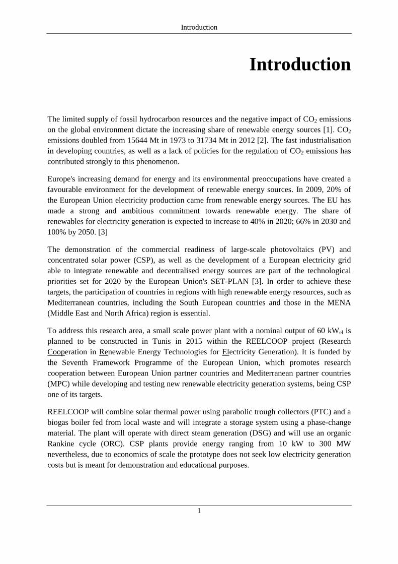
Fig.1.3 and Fig.1.4 show schematic diagrams to compare the configuration of a solar thermal plant with a conventional system and a solar power plant with DSG. Even though DSG concept is less complex, the real challenge is the presence of an inhomogeneous temperature on the circumference of the absorber due to a stratified flow in the tubes, leading to material stress [17].

Fig. 1.3 Schematic representation of a parabolic trough CSP plant with a conventional configuration [17]


7

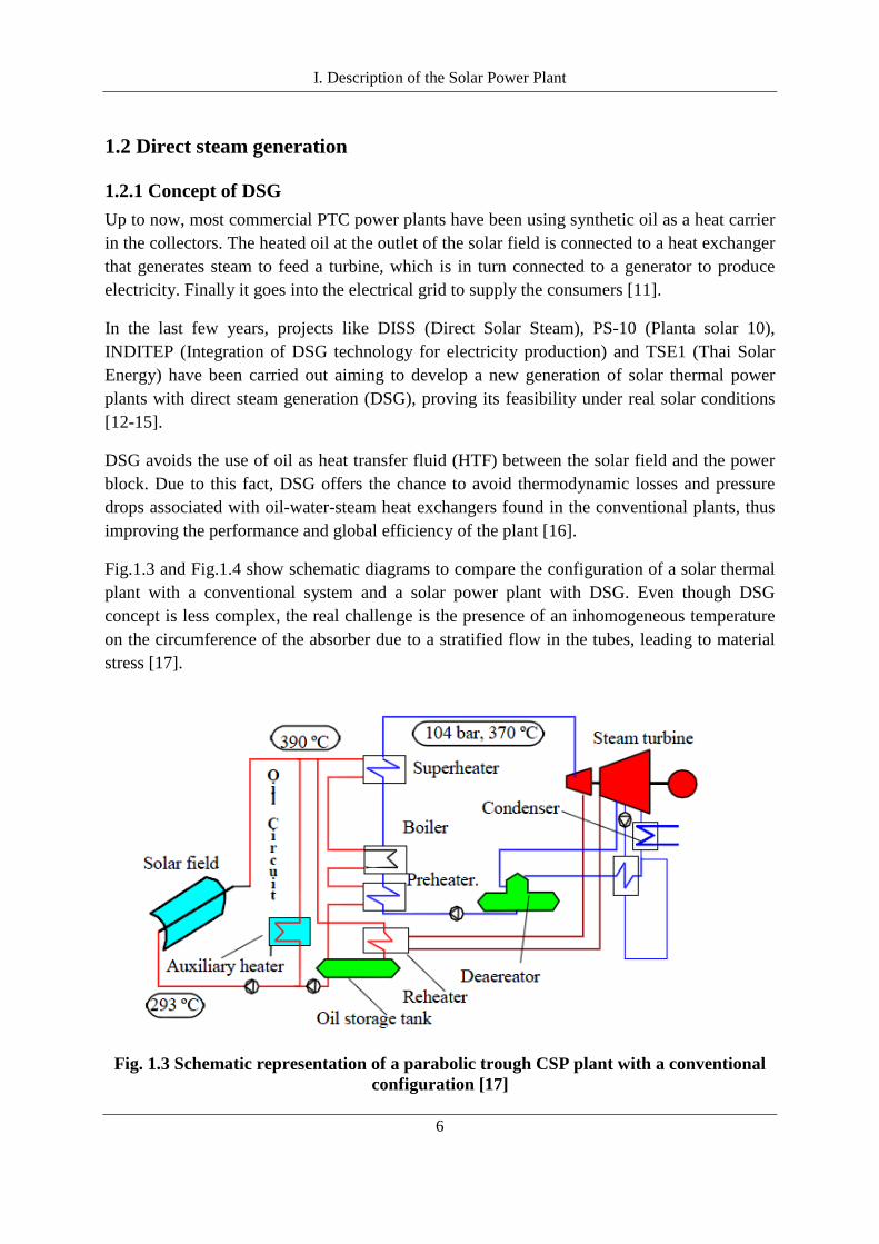
Fig. 1.4 Schematic representation of a parabolic trough CSP plant with direct steam generation [17]

Solar DSG has several advantages: higher steam temperatures and as a consequence higher steam cycle efficiencies can be reached. Replacement of the oil by DSG results not only in lower investment and operating costs, but also reduces the environmental risk and fire hazard in case of leaks [18]. For these reasons using DSG results in an innovative characteristic of the project promising an option to further the competitiveness of the PTC technology. On the other hand, one critical technical problem in DSG is the two-phase flow (water-steam) in the absorber tubes of the solar collectors. This issue involves the solar field controllability and stability, the absorber pipe stresses and consequently, their performance and durability.

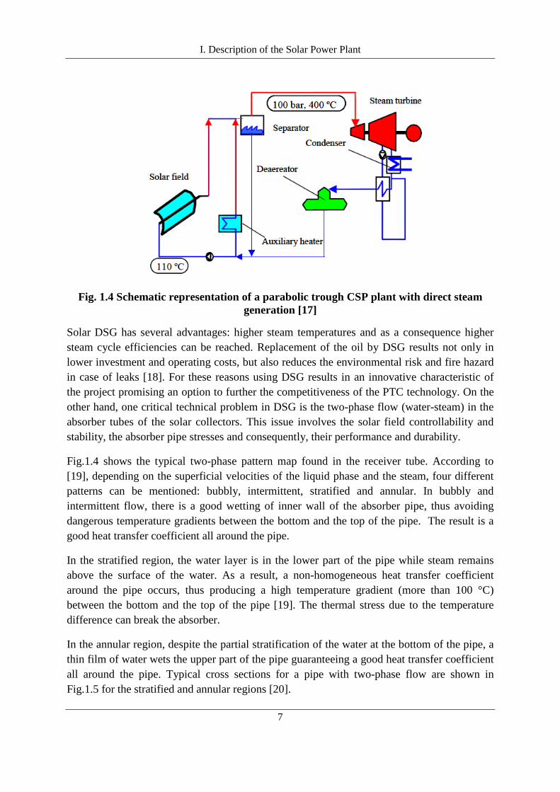
Fig.1.4 shows the typical two-phase pattern map found in the receiver tube. According to [19], depending on the superficial velocities of the liquid phase and the steam, four different patterns can be mentioned: bubbly, intermittent, stratified and annular. In bubbly and intermittent flow, there is a good wetting of inner wall of the absorber pipe, thus avoiding dangerous temperature gradients between the bottom and the top of the pipe. The result is a good heat transfer coefficient all around the pipe.

In the stratified region, the water layer is in the lower part of the pipe while steam remains above the surface of the water. As a result, a non-homogeneous heat transfer coefficient around the pipe occurs, thus producing a high temperature gradient (more than 100 °C) between the bottom and the top of the pipe [19]. The thermal stress due to the temperature difference can break the absorber.

In the annular region, despite the partial stratification of the water at the bottom of the pipe, a thin film of water wets the upper part of the pipe guaranteeing a good heat transfer coefficient all around the pipe. Typical cross sections for a pipe with two-phase flow are shown in Fig.1.5 for the stratified and annular regions [20].


8

Fig. 1.5 Two-phase flow pattern map for a horizontal pipe [19]

According to [11], a minimum feed flow rate must be guaranteed in the solar field to avoid high temperature gradients in the cross section of the absorbers tubes, so that acceptable flow conditions can be achieved. In order to accomplish this, three different operation modes for producing steam in DSG can be chosen. They are described as follows.

1.2.2 Operation modes of DSG According to [18], steam may be produced in the absorber tubes of PTC in three different ways without causing dangerous temperature gradients. Every option demands different investment costs and offers variants for the overall behaviour of the power plant during solar transients. These three options are:

a) Once-trough mode

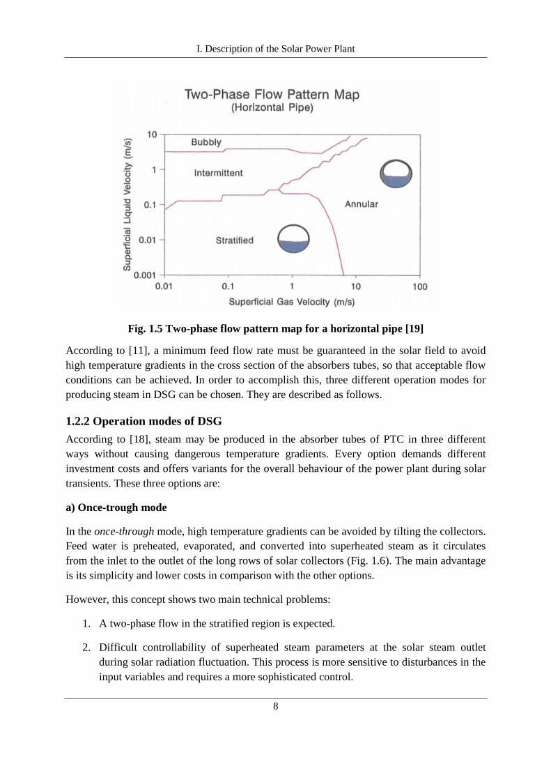
In the once-through mode, high temperature gradients can be avoided by tilting the collectors. Feed water is preheated, evaporated, and converted into superheated steam as it circulates from the inlet to the outlet of the long rows of solar collectors (Fig. 1.6). The main advantage is its simplicity and lower costs in comparison with the other options.

However, this concept shows two main technical problems:

1. A two-phase flow in the stratified region is expected.

2. Difficult controllability of superheated steam parameters at the solar steam outlet during solar radiation fluctuation. This process is more sensitive to disturbances in the input variables and requires a more sophisticated control.


9

Fig. 1.6 Schematic diagram of the once-trough mode (modified from [18])

To solve this latter, an injection process was developed.

b) Injection mode

In the injection mode, the collectors are horizontal and small amounts of water are injected along the row of collectors (Fig. 1.7). By keeping the mass flow in the absorber pipes above a threshold level, high temperature gradients may be avoided. Since the individual control of each nozzle allows injecting the exact amount of water to be evaporated before the next injection, temperature and pressure of the superheated steam at the solar field outlet are easy to control. The relative simple control is the main advantage of the injection system. On the other hand, it is more complex and expensive due to the required additional components such as piping, valves and measurement and control system.

Fig. 1.7 Schematic diagram of the injection mode (modified from [18])

c) Recirculation mode

In recirculation mode, the solar field is subdivided into a preheating/evaporation section and a superheating section by a steam drum. In this configuration, the inlet feed-water flow rate is much higher than the steam production rate of the system. A water-steam separator is located at the end of the evaporating section. The steam is separated from the water by the steam drum, and the remaining water is sent back into the solar field inlet by a recirculation pump (Fig. 1.8). The high mass flow rates and low vapour content guarantee a good wetting of the absorber tube, making stratification more difficult. This type of system can be controlled well,


10

but the excess water that has to be recirculated and the pump necessary for it increases system parasitic loads and costs.

Fig. 1.8 Schematic diagram of the recirculation mode [modified from [18]]

According to a comparison of the three DSG processes done by [21], despite the lower investment costs and simplicity of the once-trough concept, the recirculation mode is the most feasible option for commercial application, regarding financial, technical, operation and maintenance (O&M) related parameters.

A summary of the advantages and disadvantages of the three different configurations for DSG is shown in the following table.

Table 1.1 Comparison of the three operation modes for DSG [21]

Once-trough Injection Recirculation

Advantages

Least costs Good Controllability Good flow stability

Least complexity Flow stability equally good Good controllability

Good performance

Disadvantages

Controllability Higher complexity Higher complexity

Flow Stability Higher investment costs Higher investment costs

Higher parasitic loads

The description of the recirculation mode explained above is only valid when superheated steam is produced. For the saturated steam cycle, the collectors after the steam drum are not needed. This is of particular interest for the present work because the solar field is responsible of supplying saturated steam to the ORC. This will be discussed in the next subchapter.


11

1.3 Description of the power plant In section 1.1, a general description of the power plant with its main characteristics was presented. In the following sections the main subsystems and hydraulic circuit, will be discussed more in detail.

1.3.1 Solar field The solar field is composed of 12 PTMx/hp-36 solar collectors manufactured by the Italian company Soltigua. Each collector is composed of six parabolic modules with an aperture width of 2.37 m and a length of 5.95 m, that is a total of 428.4 m for the 12 collectors with a distance of 7.2 m between the rows. The inner absorber pipe diameter is 38.4 mm. Due to the thermal energy required to drive the ORC and to limitations of budget within the project a solar field with a net collector surface of 979 m² has been determined.

The collectors utilise glass and silver mirrors. The receiver consists of a non-evacuated absorber tube with an outer glass tube. Concerning the tracking and control system, each collector has an independent drive system, which tracks the sun during the day, managed by an on-board electric control panel. A temperature sensor is connected to the control in order to detect and avoid excess temperatures. All on-board control panels are wired to a general control panel, which controls the whole solar field and connects it to further safety sensors such as wind and radiation sensors. The solar field can run completely automatically and is controlled by an industrial PLC (programmable logic controller). The PLC starts tracking in the morning and controls all working parameters, to detect alarms or unusual situations. In such cases, the system exits its automatic cycle to go back to a stowing and safe position. The working principle of the collectors is shown in Fig.1.9.

Fig. 1.9 PTMx collector’s working principle [22]

In order to avoid a high pressure drop in the solar field, various configurations combining collector rows in parallel and in series were investigated and provided by Abdallah Khenissi from studies carried out at DLR in May 2014 using the software Ebsilon. These studies considered the thermo hydraulic parameters of the two-phase flow and their influence on the performance of the collectors. Results showed that the higher the number of installed parallel loops, the lower the pressure losses. In other words, a solar field consisting of 12 collectors in series present the highest pressure drop while the lowest pressure drop is obtained when a


12

configuration of 12 parallel loops is chosen [23]. These simulations are out of the scope of this thesis.

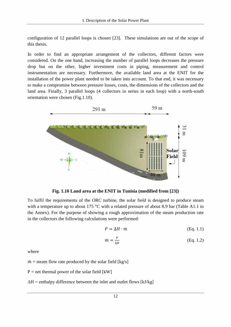
In order to find an appropriate arrangement of the collectors, different factors were considered. On the one hand, increasing the number of parallel loops decreases the pressure drop but on the other, higher investment costs in piping, measurement and control instrumentation are necessary. Furthermore, the available land area at the ENIT for the installation of the power plant needed to be taken into account. To that end, it was necessary to make a compromise between pressure losses, costs, the dimensions of the collectors and the land area. Finally, 3 parallel loops (4 collectors in series in each loop) with a north-south orientation were chosen (Fig.1.10).

Fig. 1.10 Land area at the ENIT in Tunisia (modified from [23])

To fulfil the requirements of the ORC turbine, the solar field is designed to produce steam with a temperature up to about 175 °C with a related pressure of about 8.9 bar (Table A1.1 in the Annex). For the purpose of showing a rough approximation of the steam production rate in the collectors the following calculations were performed:

𝑃 = ∆𝐻 ∙ �� (Eq. 1.1)

�� = 𝑃∆𝐻

(Eq. 1.2)

where

�� = steam flow rate produced by the solar field [kg/s]

P = net thermal power of the solar field [kW]

ΔH = enthalpy difference between the inlet and outlet flows [kJ/kg]


13

To get a rough value of the net thermal power of the solar field, a direct normal irradiance (DNI) of 750 W/m2 and a total collector area of 980 m2 were considered. Furthermore, an efficiency 𝜂𝑆𝐹 = 60% for the solar field was assumed contemplating the thermal and cosine losses. Thus, an estimation of the net thermal power of the field is

𝑃 = 𝐷𝑁𝐼 ∗ 𝐴𝑟𝑒𝑎 ∗ 𝜂 (Eq. 1.3)

𝑃 = 750𝑊𝑚2 ∗ 980 𝑚2 ∗ 0.60

𝑃 = 441 𝑘𝑊

The ΔH of the solar field corresponds to the enthalpy difference between the specific enthalpies of the steam at the inlet of the turbine and the condensate at the outlet. A temperature of 175 °C for the steam at the inlet and 80 °C for the condensate at the outlet are assumed. The associated specific enthalpies are ho = 2773 kJ/kg and hi = 334 kJ/kg for the steam and condensate, respectively. Thus ΔH can be calculated as follows:

ℎ𝑖 = 335𝑘𝐽𝑘𝑔

ℎ𝑜 = 2773𝑘𝐽𝑘𝑔

∆𝐻 = ℎ𝑜 − ℎ𝑖 (Eq. 1.4)

∆𝐻 = 2438𝑘𝐽𝑘𝑔

Substituting ΔH and P in Eq. 1.2 we get the mass flow rate of the steam produced in the total

�� =441 𝑘𝑊

2438 𝑘𝐽𝑘𝑔

�� = 𝟎.𝟏𝟖𝒌𝒈𝒔

or

�� = 𝟔𝟓𝟏𝒌𝒈𝒉

Approximately a total mass flow rate of 0.18 kg/s of steam will be produced in the solar field in nominal operation.


14

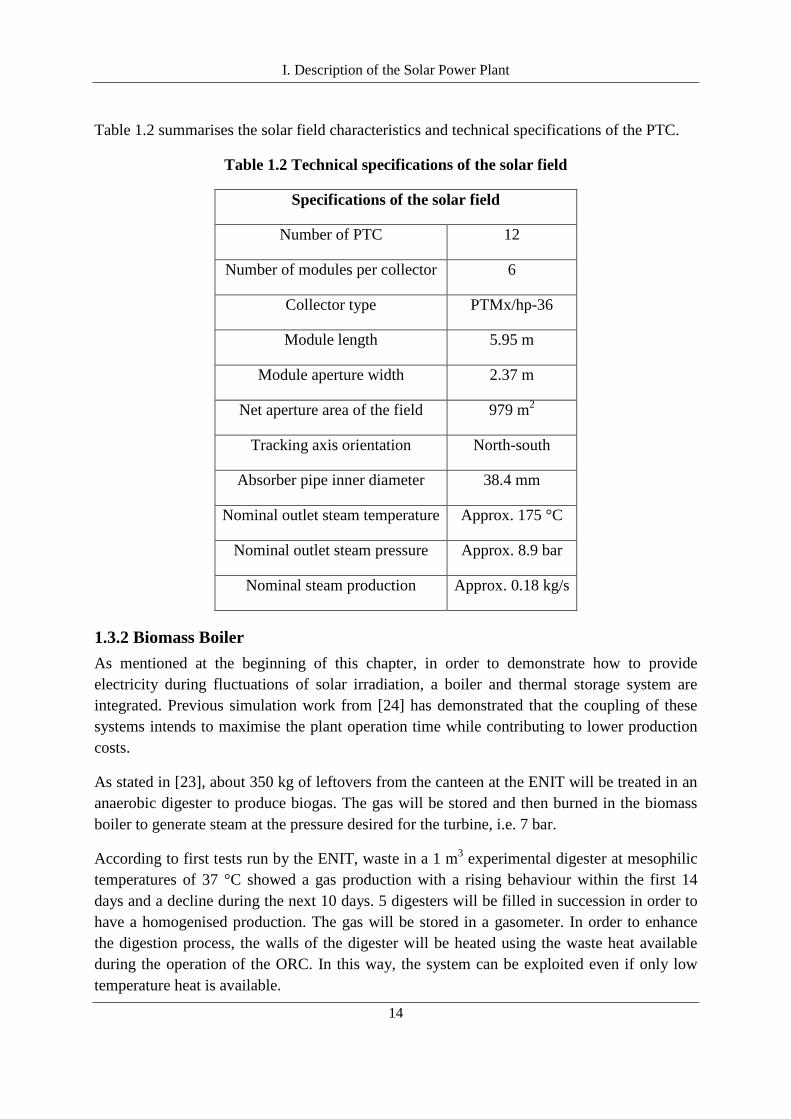
Table 1.2 summarises the solar field characteristics and technical specifications of the PTC.

Table 1.2 Technical specifications of the solar field

Specifications of the solar field

Number of PTC 12

Number of modules per collector 6

Collector type PTMx/hp-36

Module length 5.95 m

Module aperture width 2.37 m

Net aperture area of the field 979 m2

Tracking axis orientation North-south

Absorber pipe inner diameter 38.4 mm

Nominal outlet steam temperature Approx. 175 °C

Nominal outlet steam pressure Approx. 8.9 bar

Nominal steam production Approx. 0.18 kg/s

1.3.2 Biomass Boiler As mentioned at the beginning of this chapter, in order to demonstrate how to provide electricity during fluctuations of solar irradiation, a boiler and thermal storage system are integrated. Previous simulation work from [24] has demonstrated that the coupling of these systems intends to maximise the plant operation time while contributing to lower production costs.

As stated in [23], about 350 kg of leftovers from the canteen at the ENIT will be treated in an anaerobic digester to produce biogas. The gas will be stored and then burned in the biomass boiler to generate steam at the pressure desired for the turbine, i.e. 7 bar.

According to first tests run by the ENIT, waste in a 1 m3 experimental digester at mesophilic temperatures of 37 °C showed a gas production with a rising behaviour within the first 14 days and a decline during the next 10 days. 5 digesters will be filled in succession in order to have a homogenised production. The gas will be stored in a gasometer. In order to enhance the digestion process, the walls of the digester will be heated using the waste heat available during the operation of the ORC. In this way, the system can be exploited even if only low temperature heat is available.


15

Currently, organic waste represents a health problem and a natural hazard in Tunis. Thus, the hybridization of the solar- and bioenergy will not only be used for demonstration of the technology but it will also contribute to the improvement of environmental and living conditions for the population.

1.3.3 Storage system Due to the hybridization of the solar field with the biogas boiler, the need for large storage devices to operate the plant during the night can be avoided. Simultaneously, the storage system will be able to provide the required energy to compensate the biogas boiler start-up and short transients.

The steam produced in the solar field is at a temperature between 160 °C and 175 °C and the required steam inlet temperature for the ORC under nominal operation is about 170 °C. For this reason, the exceeding temperature will be used to load the storage system.

The storage system works utilising a PCM, which is a substance with a high heat of fusion. In other words, when melting and solidifying at a certain temperature, it is capable of storing and releasing large amounts of energy. Heat is absorbed or released when the material changes from solid to liquid due to the latent energy and vice versa. According to [25], latent heat storage is advantageous for evaporation processes.

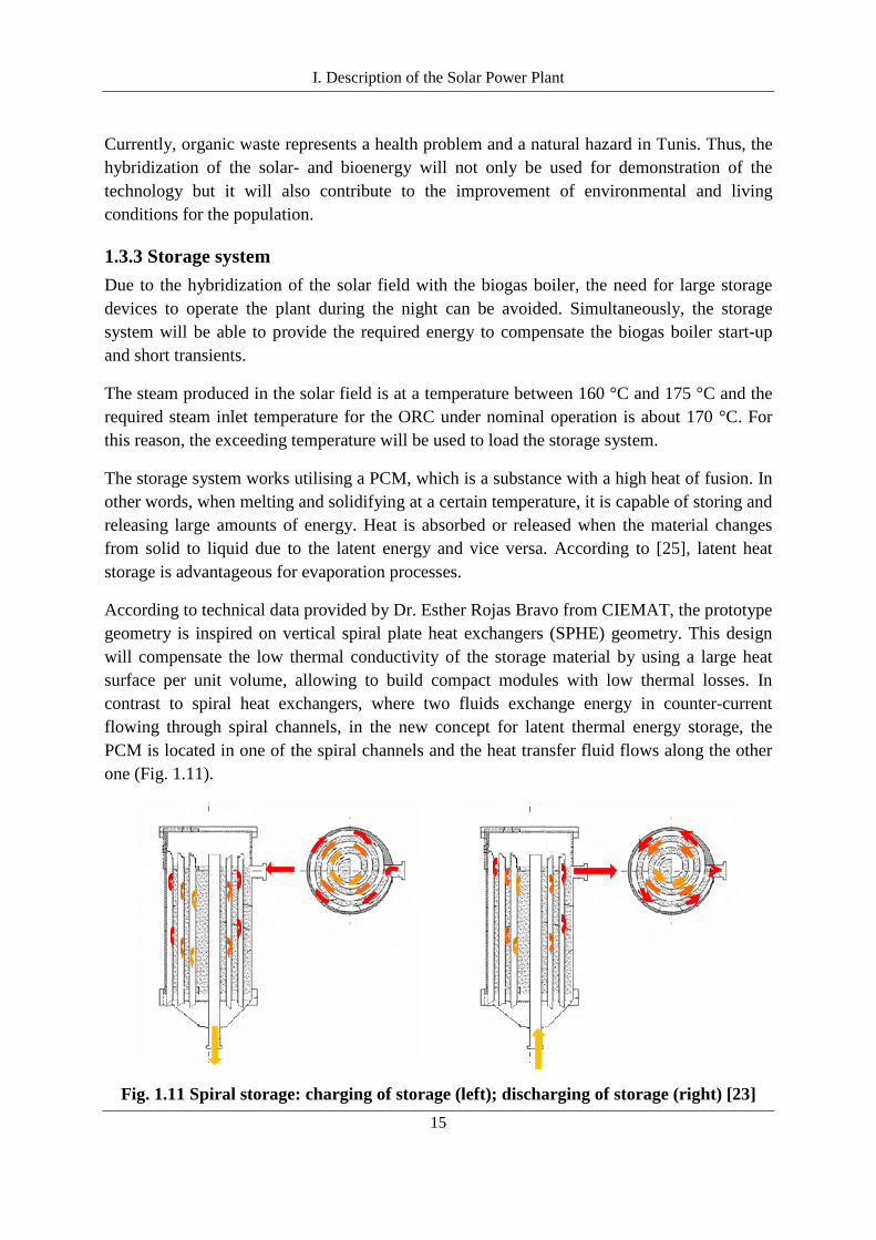
According to technical data provided by Dr. Esther Rojas Bravo from CIEMAT, the prototype geometry is inspired on vertical spiral plate heat exchangers (SPHE) geometry. This design will compensate the low thermal conductivity of the storage material by using a large heat surface per unit volume, allowing to build compact modules with low thermal losses. In contrast to spiral heat exchangers, where two fluids exchange energy in counter-current flowing through spiral channels, in the new concept for latent thermal energy storage, the PCM is located in one of the spiral channels and the heat transfer fluid flows along the other one (Fig. 1.11).

Fig. 1.11 Spiral storage: charging of storage (left); discharging of storage (right) [23]

http://en.wikipedia.org/wiki/Heat_of_fusion


16

During the charging of the storage system, the saturated steam from the solar field goes into the storage module through the lateral opening and flows through the spiral channel from the biggest diameter to the smallest one. The steam gives its energy by melting the PCM, placed in the alternate spiral channel and condensates. During discharge, the process runs in the opposite direction. Saturated water enters the storage module from the bottom opening and flows through the spiral channel from the smallest diameter to the biggest one. The water gains energy and evaporates by solidifying the liquid PCM, and exits the module through the lateral upper opening as saturated steam [23].

There are several reasons to take the storage system and the biogas boiler into account as support systems for the solar field-power block coupling. If only the auxiliary biogas boiler was considered, the number of operation hours at nominal conditions would decrease. On the other hand, if only thermal storage was considered, there would be non-isolation intervals in which the ORC would have to work at part load conditions, due to the storage system inertia [26]. It is expected that the auxiliary boiler considered can face up to these isolation fluctuations, smoothing out isolation changes for steady cycle operation.

The thermal storage system and the biogas boiler are key elements for guaranteeing steady conditions at the power cycle inlet and solar power plant output. Therefore, it is of great importance to investigate the coupling of these systems, their performance and reliability to maximise the plant operation. Nevertheless, these systems are out of the scope of this work.

1.3.4 Organic Rankine cycle Initially, a steam turbine of the company Voith had been considered for the project nevertheless, the required temperature (above 300 °C) of the superheated steam needed to run the turbine resulted in a technical challenge for the project, especially for the collectors, as explained in section 1.1. For this reason, a more viable alternative was found, integrating an ORC within the appropriate power range i.e. 60 kWel, requiring an inlet temperature of 175 °C. The turbine that suffices these characteristics is manufactured by the Italian company Zuccato Energia. In the following sections, the general concept of ORC will be explained and the description of the ORC in the power plant will be detailed.

General description of ORC

Electrical power is usually generated in processes based on the Clausius-Rankine cycle with water-steam as a working fluid. The organic Rankine cycle (ORC) is a Clausius-Rankine cycle in which an organic working fluid is used instead of water-steam. In comparison to water, organic fluids are advantageous when the maximum temperature is low and/or the power plant is small. At low temperatures, organic fluids lead to higher cycle efficiency than water. For this reason, it has become popular for energy production processes in small plants in the last years [27].


17

In the ORC, a pump compresses the organic working fluid forcing it through a regenerator (heat exchanger). The regenerator allows the preheating of the liquid working fluid by cooling down the expanded vapour. The preheated working fluid is then evaporated, superheated and expanded in a turbine, which drives a generator, converting its enthalpy into work. The cooled down vapour is condensed in a condenser. The liquid available at the condenser outlet is pumped back to the upper heat exchangers and a new cycle begins. If low temperature heat is used for driving the ORC, the condenser is cooled down by means of cooling water. Fig. 1.12 shows the main components of the ORC [28].

Fig. 1.12 Main components of ORC [28]

The process described above is shown in a T–S diagram in Fig 1.13. 0-1 Compression in feed pump; 1-2 preheating; 2-3 evaporation; 3-4 superheating; 5-6 cooling-down; 6-0 condensation.

Fig. 1.13 T-S diagram for ORC (modified from [28])


18

The ORC can work with saturated steam and no higher superheating is necessary to avoid liquid in the exhaust vapour. The reason for this is that in contrast to water, the expansion in the turbine ends for most organic fluids not in the wet steam regime but in the gas phase above condenser temperature. Higher superheating of the vapour is favourable for higher efficiencies, but because of the low heat exchange coefficients, very large heat exchangers would be needed, making the system much more expensive [28].

The selection of the working fluid plays a significant role for the use of ORC process and is determined by the application and the source heat level [29]. According to [30], in order to identify the most suitable organic fluids, several general criterions have to be taken into consideration, including thermodynamic properties; stability of the fluid and compatibility with materials in contact; safety, health and environmental aspects; availability and costs.

Although investigated since the 1880’s, one of the main reasons why the construction of new ORC plants increases is the fact that it is a proven technology for decentralized applications for the production of power of few kWel up to 1 MWel. The electrical efficiency of the ORC process lies between 6 and 17%. However, even if the efficiency is low, there are some advantages, for instance, the fact that no maintenance for the system and not so high pressures are required, lower safety measures are needed, leading to low costs. As mentioned before, for many organic fluids the expansion of the turbine ends in the region of superheated vapour. This avoids drop erosion and allows a reliable operation and a fast start up of the cycle. The efficiency of an ORC turbine is up to 85% and it has an outstanding part load behaviour [28]. For all these reasons, ORC are suitable for small scale solar thermal power plants.

Description of the power block of the plant

According to technical data provided by Zuccato Energia and as stated in [23], the nominal gross efficiency of the ORC reaches 13 to 15%. Initially, the units of the company were meant for exploiting waste heat gas or pressurised water therefore, the heat exchangers and control needed to be adapted.

The steam at 175 °C is fed to the system through a 2-way power valve. It reaches the two heat braze-welded exchangers and then it goes back to the source as condensate at 80 °C (Fig 1.14). As reported by [23], the turbine's control system allows variable speed, thus optimising the electrical yield during partial load conditions. Furthermore, the compact unit allows easy maintenance operations and thanks to the use of a new generator design with lower friction losses and better cooling performance, a high electrical yield is achieved.


19

Fig. 1.14 Power block of the power plant

In contrast to the waste heat temperature of steam turbines at about 100 °C or more, in ORC the waste heat temperature varies depending on the temperature range of operation of the turbine. For the inlet temperature necessary to drive this turbine, i.e. about 175 °C, a high amount of low temperature waste heat between 40 °C and 50 °C would be available. Even though a small share of this heat would be utilised to enhance the biomass gasification process, a high amount of heat would dissipate. The latter represents a disadvantage with respect to the overall efficiency of the plant. For economical reasons, a higher utilisation of the waste heat is recommended. To that end, it is necessary to run the ORC at higher outlet temperatures, so that an industrial consumer or cooling machine can be supplied. This is foreseen as an outlook of the technology for future stages.

1.4 Description of the hydraulic circuit In the following sections, the hydraulic circuit of the plant will be discussed, including a description of the elements involved, dimensioning and pressure drops.

1.4.1 Recirculation mode and steam drum of the plant Based on the comparison of the different operation modes for DSG, the recirculation mode is the most feasible option for commercial applications, regarding financial, technical and O&M related parameters. Furthermore, the recirculation mode offers a better flow stability and controllability than those from the once-trough mode. Besides that, the recirculation mode in DSG is a proven technology that has been successfully tested and demonstrated in installations before. As already discussed in 1.2.1, by supplying the collectors with a higher mass flow of water than the rate of steam produced the recirculation mode avoids thermal and mechanical stresses in the absorbers due to dry-out. For these reasons, the recirculation mode was chosen for the operation of the plant taking, however, into consideration the higher costs implied.


20

At nominal operation, sub-cooled water at about 148 °C is pumped to the collector field to be evaporated, reaching a temperature of 175 °C. The two-phase flow coming out from the collectors goes into the steam drum. The steam drum is a water-steam separator vessel, whose one of its functions is to separate the saturated steam from the water-steam mixture. The steam drum separates the saturated steam in the two-phase flow and sends it to two plate heat exchangers to transfer the heat to the power block. In the power block, as described before, an ORC takes place, evaporating an organic working fluid to drive the turbine, converting the heat into work to run a generator and produce electricity. The steam is condensed and sub-cooled by the heat exchangers to 80 °C and then is pumped back by the so-called feed water pump and start the cycle all over again. Meanwhile, the saturated water in the steam drum is sent back to the solar field by a recirculation pump at a temperature of about 175 °C, working in this way as a buffer and helping to keep the thermal inertia of the system. Before going into the solar field, the saturated water at 175 °C coming from the steam drum mixes with the sub-cooled water at 80 °C, condensed by the heat exchangers, resulting in the initial 148 °C. Furthermore, the steam drum is also able to quickly supply a high amount of water in case of a fast radiation drop, in order to fill the absorber tubes with water.

For this complete water-steam cycle, the two pumps mentioned (i.e. the recirculation and the feed water pumps), as well as the steam drum are essential. For the steam drum, a vertical vessel with a capacity of 200 litres was determined. Nevertheless, one of 500 litres was chosen instead for redundancies. The volume of the steam drum is relevant for the dimensioning of the expansion tank described below. The selection of the pumps depends on the pressure drop to be compensated and it will be described in later sections.

1.4.2 Closed loop and expansion tank In order to avoid air coming into the system, causing thus corrosion, the power plant is planned as a closed loop steam/condensate system instead of the typical open process steam supplies. This means that the water is re-used time and again in a loop and water is only added to make up for leaks in the system.

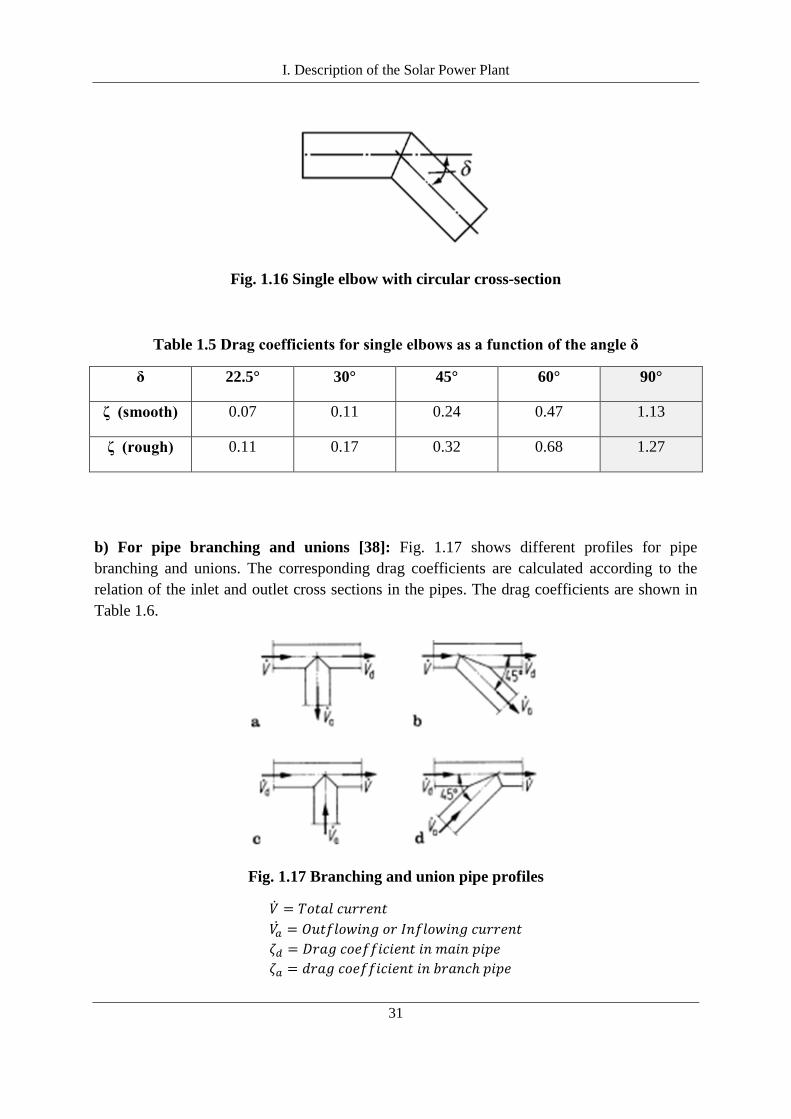
Another measure to avoid air in the installation is filling it with water in periods when it is not operating. At night or during transients, the steam is condensed and since the density of liquid water is about 1000 times lower than that of steam, the volume of the fluid in the system (including piping and steam drum) would decrease considerably. As a consequence, a pressure below 1 bar would be reached, leading to a possible undesired air inlet. To prevent this, an expansion tank using a nitrogen cushion, with a pressure slightly above ambient pressure, would push water towards the system filling it completely and ensuring no air can go in. Inversely, during start-up and at nominal operation, the steam produced would displace the water, pushing it towards the expansion tank, where it would be stored. The steam piping is shown in red in Fig. 1.19. In order to take all the water displaced, the expansion tank needs to be dimensioned accordingly. To that end, several factors need to be considered when dimensioning the expansion tank. The derivation of the calculations is shown below.


21

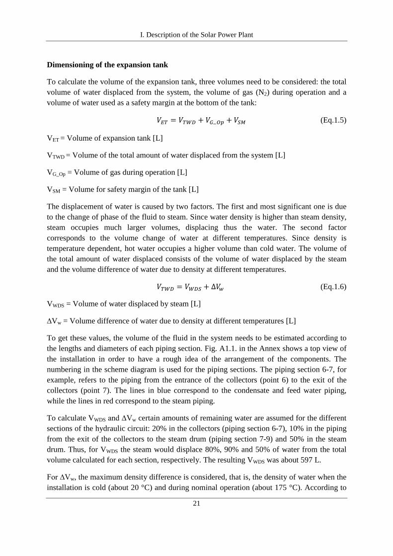
Dimensioning of the expansion tank

To calculate the volume of the expansion tank, three volumes need to be considered: the total volume of water displaced from the system, the volume of gas (N2) during operation and a volume of water used as a safety margin at the bottom of the tank:

𝑉𝐸𝑇 = 𝑉𝑇𝑊𝐷 + 𝑉𝐺−𝑂𝑝 + 𝑉𝑆𝑀 (Eq.1.5)

VET = Volume of expansion tank [L]

VTWD = Volume of the total amount of water displaced from the system [L]

VG_Op = Volume of gas during operation [L]

VSM = Volume for safety margin of the tank [L]

The displacement of water is caused by two factors. The first and most significant one is due to the change of phase of the fluid to steam. Since water density is higher than steam density, steam occupies much larger volumes, displacing thus the water. The second factor corresponds to the volume change of water at different temperatures. Since density is temperature dependent, hot water occupies a higher volume than cold water. The volume of the total amount of water displaced consists of the volume of water displaced by the steam and the volume difference of water due to density at different temperatures.

𝑉𝑇𝑊𝐷 = 𝑉𝑊𝐷𝑆 + ∆𝑉𝑤 (Eq.1.6)

VWDS = Volume of water displaced by steam [L]

∆Vw = Volume difference of water due to density at different temperatures [L]

To get these values, the volume of the fluid in the system needs to be estimated according to the lengths and diameters of each piping section. Fig. A1.1. in the Annex shows a top view of the installation in order to have a rough idea of the arrangement of the components. The numbering in the scheme diagram is used for the piping sections. The piping section 6-7, for example, refers to the piping from the entrance of the collectors (point 6) to the exit of the collectors (point 7). The lines in blue correspond to the condensate and feed water piping, while the lines in red correspond to the steam piping.

To calculate VWDS and ∆Vw certain amounts of remaining water are assumed for the different sections of the hydraulic circuit: 20% in the collectors (piping section 6-7), 10% in the piping from the exit of the collectors to the steam drum (piping section 7-9) and 50% in the steam drum. Thus, for VWDS the steam would displace 80%, 90% and 50% of water from the total volume calculated for each section, respectively. The resulting VWDS was about 597 L.

For ∆Vw, the maximum density difference is considered, that is, the density of water when the installation is cold (about 20 °C) and during nominal operation (about 175 °C). According to


22

Table A1.2, the densities are 998.2 kg/m3 and 897.3 kg/m3, respectively. As the mass remains the same, the calculation ∆Vw is derived as follows:

𝑚𝑐𝑜𝑙𝑑 = 𝑚ℎ𝑜𝑡 (Eq.1.7)

𝜌 = 𝑚𝑉

(Eq.1.8)

𝑉𝑐𝑜𝑙𝑑 ∙ 𝜌𝑐𝑜𝑙𝑑 = 𝑉ℎ𝑜𝑡 ∙ 𝜌ℎ𝑜𝑡 (Eq.1.9)

𝑉ℎ𝑜𝑡 = 𝑉𝑐𝑜𝑙𝑑 ∙𝜌𝑐𝑜𝑙𝑑𝜌ℎ𝑜𝑡

∆𝑉𝑤 = 𝑉ℎ𝑜𝑡 − 𝑉𝑐𝑜𝑙𝑑

∆𝑉𝑤 = 𝑉𝑐𝑜𝑙𝑑 − 𝑉𝑐𝑜𝑙𝑑 ∙𝜌𝑐𝑜𝑙𝑑𝜌ℎ𝑜𝑡

(Eq.1.10)

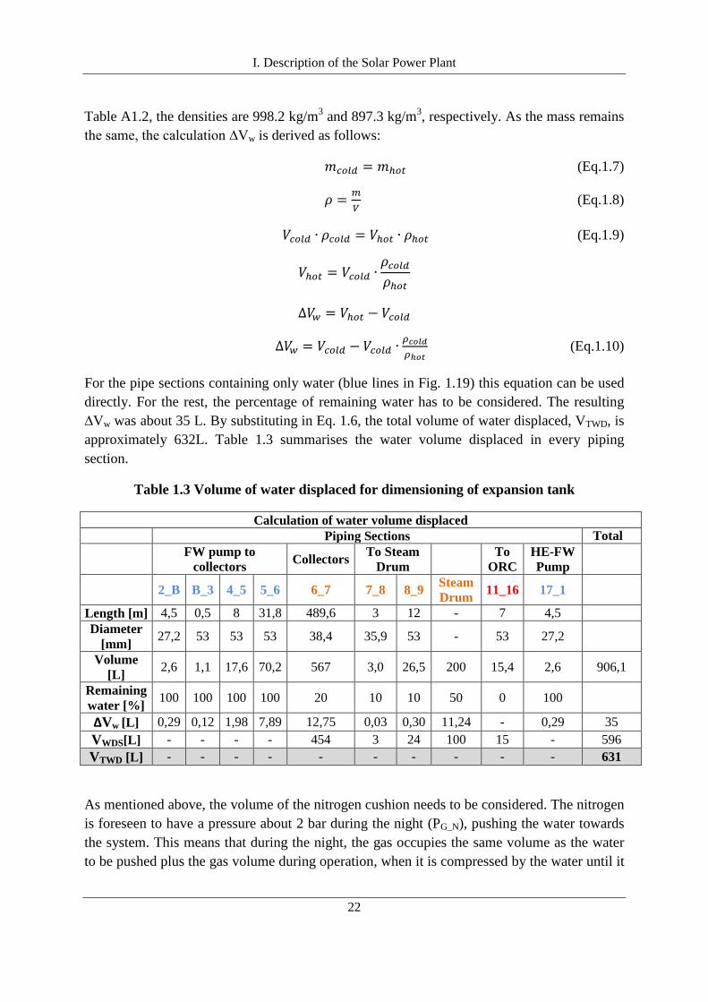
For the pipe sections containing only water (blue lines in Fig. 1.19) this equation can be used directly. For the rest, the percentage of remaining water has to be considered. The resulting ∆Vw was about 35 L. By substituting in Eq. 1.6, the total volume of water displaced, VTWD, is approximately 632L. Table 1.3 summarises the water volume displaced in every piping section.

Table 1.3 Volume of water displaced for dimensioning of expansion tank

Calculation of water volume displaced Piping Sections Total

FW pump to

collectors Collectors To Steam Drum

To ORC

HE-FW Pump

2_B B_3 4_5 5_6 6_7 7_8 8_9 Steam

Drum 11_16 17_1 Length [m] 4,5 0,5 8 31,8 489,6 3 12 - 7 4,5 Diameter

[mm] 27,2 53 53 53 38,4 35,9 53 - 53 27,2 Volume

[L] 2,6 1,1 17,6 70,2 567 3,0 26,5 200 15,4 2,6 906,1

Remaining water [%] 100 100 100 100 20 10 10 50 0 100 ∆Vw [L] 0,29 0,12 1,98 7,89 12,75 0,03 0,30 11,24 - 0,29 35 VWDS[L] - - - - 454 3 24 100 15 - 596 VTWD [L] - - - - - - - - - - 631

As mentioned above, the volume of the nitrogen cushion needs to be considered. The nitrogen is foreseen to have a pressure about 2 bar during the night (PG_N), pushing the water towards the system. This means that during the night, the gas occupies the same volume as the water to be pushed plus the gas volume during operation, when it is compressed by the water until it


23

reaches the same pressure, that is, about 8.9 bar (PG_Op). Thus, the relation between the volume and pressure of the gas at night and during operation is:

𝑉𝐺−𝑂𝑝∗𝑉𝑇𝑊𝐷

= 𝑃𝐺−𝑁𝑃𝐺−𝑂𝑝

(Eq.1.11)

𝑉𝐺−𝑂𝑝∗ =𝑃𝐺−𝑁𝑃𝐺−𝑂𝑝

∙ 𝑉𝑇𝑊𝐷

𝑉𝐺−𝑂𝑝∗ =2𝑏𝑎𝑟

8.9𝑏𝑎𝑟∙ 631𝐿

𝑉𝐺−𝑂𝑝∗ = 142𝐿

Taking into account the thermal expansion of the gas, and assuming it is an ideal gas, the volume would be:

𝑉𝐺−𝑂𝑝 = 𝑇𝐺−𝑂𝑝𝑇𝐺−𝑁

∙ 𝑉𝐺−𝑂𝑝∗ (Eq.1.12)

𝑉𝐺−𝑂𝑝 =(175 + 273.15)𝐾(20 + 273.15)𝐾

∙ 142𝐿

𝑉𝐺−𝑂𝑝 = 217𝐿

Finally, a safety margin at the bottom of the tank has to be considered in order to guarantee that there is always remaining water in the tank and consequently, no nitrogen can directly go into the system. The water volume for this safety margin was chosen to be 100 L. By substituting the values gotten above in Eq.1.6, the resulting volume of the expansion tank is:

𝑉𝐸𝑇 = 𝑉𝑇𝑊𝐷 + 𝑉𝐺−𝑂𝑝 + 𝑉𝑆𝑀

𝑉𝐸𝑇 = 632𝐿 + 217𝐿 + 100𝐿

𝑽𝑬𝑻 ≅ 𝟗𝟕𝟎 𝑳

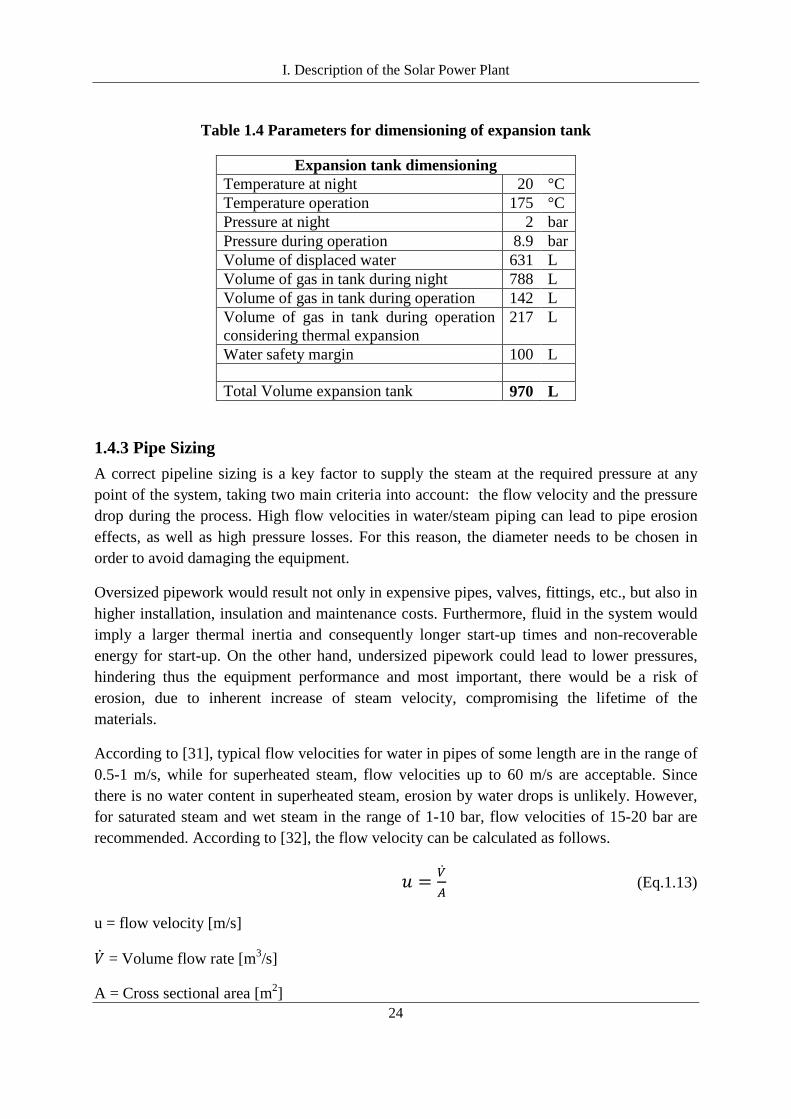
Table 1.4 summarises the volumes considered for the dimensioning of the expansion tank.


24

Table 1.4 Parameters for dimensioning of expansion tank

Expansion tank dimensioning Temperature at night 20 °C Temperature operation 175 °C Pressure at night 2 bar Pressure during operation 8.9 bar Volume of displaced water 631 L Volume of gas in tank during night 788 L Volume of gas in tank during operation 142 L Volume of gas in tank during operation considering thermal expansion

217 L

Water safety margin 100 L Total Volume expansion tank 970 L

1.4.3 Pipe Sizing A correct pipeline sizing is a key factor to supply the steam at the required pressure at any point of the system, taking two main criteria into account: the flow velocity and the pressure drop during the process. High flow velocities in water/steam piping can lead to pipe erosion effects, as well as high pressure losses. For this reason, the diameter needs to be chosen in order to avoid damaging the equipment.

Oversized pipework would result not only in expensive pipes, valves, fittings, etc., but also in higher installation, insulation and maintenance costs. Furthermore, fluid in the system would imply a larger thermal inertia and consequently longer start-up times and non-recoverable energy for start-up. On the other hand, undersized pipework could lead to lower pressures, hindering thus the equipment performance and most important, there would be a risk of erosion, due to inherent increase of steam velocity, compromising the lifetime of the materials.

According to [31], typical flow velocities for water in pipes of some length are in the range of 0.5-1 m/s, while for superheated steam, flow velocities up to 60 m/s are acceptable. Since there is no water content in superheated steam, erosion by water drops is unlikely. However, for saturated steam and wet steam in the range of 1-10 bar, flow velocities of 15-20 bar are recommended. According to [32], the flow velocity can be calculated as follows.

𝑢 = ��𝐴

(Eq.1.13)

u = flow velocity [m/s]

�� = Volume flow rate [m3/s]

A = Cross sectional area [m2]


25

In terms of the mass flow rate and the diameter of the pipes, it can also be expressed as:

𝑢 = 𝑚

𝜌∙𝜋∙𝑑24

(Eq.1.14)

ρ = density [kg/m3]

d = pipe inner diameter [m]

By choosing flow velocities in an acceptable range and according to the mass flow rates, the density associated to the temperature and nature of the fluid expected along the piping, the diameter can be then calculated.

𝑑 = � 4∙��𝜌∙𝜋∙𝑢

(Eq.1.15)

With this equation, a first calculation was done to determine the diameters, choosing the standard nominal diameters (DN). The flow velocity was calculated again to verify its suitability for the chosen diameters. For the solar field, the flow velocity and pressure losses depend on the number of parallel rows, as explained in section 1.3.1. The calculation of the pressure drop associated to each pipe section is described below. The calculations were done in Excel. The results are shown in the Annex (Table A1.3).

1.4.4 Valves, filters, steam traps, flex hoses, separators and pumps Various devices are used in the plant for several purposes including control, safety or maintenance. The devices described below are relevant for the planning and design of the hydraulic system (Fig. 1.19), mainly due to two factors: the regulating functions they perform and the pressure losses across them. The importance of the pressure losses and its calculation will be described in later sections.

Flow instabilities between parallel loops in power plants with DSG occur because one of the loops has a higher evaporation rate than the others, leading to higher pressure drops. Consequently, less water flows into that loop and more in the others, aggravating thus the effect. To deal with these flow instabilities, automatic valves for mass flow control will be used in the plant. Three parallel rows are, in fact, less likely to suffer flow instability than a larger number of parallel rows. By partially closing the valves, pressure drop can be caused in order to avoid that the fluctuations in the pressure drop lead to serious mass flow reduction in one of the loops [23].

To regulate the mass flow rate in the condensate loop, a hand valve in a bypass of the feed water pump is installed. To prevent undesired back-flow coming into the pumps, the collectors and the storage system, non-return valves are utilised. The mass flow coming from the feed water pump into the steam drum, the storage system and the biogas boiler as well as the mass flow passing through the heat exchanger are regulated by control valves by means of


26

a proportional-integral (PI) control system. The valves are opened or closed fully or partially in response to signals received from sensors that compare the current value with a set-point (desired value). The measured signals for the PI-Control are shown in dashed lines in Fig. 1.19 at the end of this chapter.

In order to remove any moisture content in the saturated steam coming from the steam drum before passing through the heat exchangers, a separator is used to collect the remaining water. The separators need to be installed at a certain height as gravity is used to cause the liquid to settle to the bottom of the vessel, where it is withdrawn to be sent to the condensate piping, in the case of this power plant.

Inversely to the separators, the steam trap ensures to collect the remaining vapour from the storage module and after the heat exchangers, letting only the condensate to pass in order to avoid cavitation in the pumps. To guarantee that no particles and other impurities contained in the water enter to the pumps, filters are installed just right before them.

In order to compensate the pressure losses along the piping system, appropriate pumps for the power plant must be determined. To that end, a feed water pump and a recirculation pump are required.

1.5 Pressure Drop To define the technical capacities of the pumps, guaranteeing a good performance and the appropriate costs, the calculation of the pressure drop in the system must be done. The following section presents the main considerations to take into account when estimating the pressure drops.

According to [31], the pressure drop in flow through pipes of circular section is given by:

Δ𝑝 = 𝜆 𝑙𝑑𝜌𝑢2

2 (Eq. 1.16)

λ = drag coefficient [-]

d = diameter of the pipe [m]

ρ = average density of the fluid [kg/m3]

u = flow velocity [m/s]

The drag coefficient λ depends on the Reynolds number:

𝑅𝑒 = 𝑢𝜌𝑑𝜂

(Eq. 1.17)

η = dynamic viscosity of the flow [Pa/s]

http://en.wikipedia.org/wiki/Gravity


27

Below the critical Reynolds number Re ≈ 2320, flow is laminar; for 2320 < Re < 4000, a transitional flow regime is considered. The flow is uncertain, showing a dual behaviour depending on the roughness of the pipe and therefore, it is unstable. For instance, it may still be laminar in tubes with smooth inner surfaces if the inflow is quite calm and the tube inlet is well finished. As the pipe comes rougher, it shifts from laminar to turbulent flow in the direction of lower Reynolds numbers, but always above the critical Reynolds number.

Pressure drop in laminar flow

For laminar flow, regardless of the roughness of the tube wall, the pressure drop can be described by the Hagen Poiseuille law:

Δ𝑝 = 32 𝜂 𝑢 𝑙𝑑2

(Eq. 1.18)

Hence, the drag coefficient λ for laminar flow can be expressed as:

𝜆 = 64𝑅𝑒

(Eq. 1.19)

It applies accurately for smooth tubes such as glass, brass, or copper tubes.

Pressure drop in turbulent flow

According to [33], for turbulent flow, λ depends on the Reynolds number and the roughness of the pipe. Therefore, these numbers play an important role for the calculation of the pressure losses in the regime above the critical Re.

Determination of the drag coefficient λ

For hydraulic smooth pipes, i.e. with Re < 65 𝑑𝑘, several approximations for the calculation of

λ can be done:

According to Blasius, the following equation is valid for 2320 < Re < 105:

𝜆 = 0.3164√𝑅𝑒4 (Eq. 1.20)

The Nikuradse equation is valid for 105 < Re < 108:

𝜆 = 0.0032 + 0.0021𝑅𝑒0.237 (Eq. 1.21)

The Herrmann equation is convenient for the range 2x104 < Re < 2x106 [31]:

𝜆 = 0.00540 + 0.3964𝑅𝑒0.3 (Eq. 1.22)


28

The Prandtl and von Kármán equation is valid for the entire turbulent regime:

𝜆 = 1

�2𝑙𝑜𝑔�𝑅𝑒√𝜆2.51 ��2 (Eq. 1.23)

Nevertheless, due to its implicit form, numerical methods are required to solve it iteratively. Alternatively, an approximation can be obtained with the following equation:

𝜆 = 0.309

�𝑙𝑜𝑔�𝑅𝑒7 ��2 (Eq. 1.24)

For hydraulic rough pipes with Re > 1300 𝑑𝑘 , λ depends only on the relative roughness 𝑑

𝑘. For

the region above the boundary curve (Fig. 1.15), Nikuradse's equation can be applied [33]:

𝜆 = 1

�2𝑙𝑜𝑔�3.71𝑑𝑘��2 (Eq. 1.25)

The boundary curve is defined by:

𝜆 = �200𝑑𝑘𝑅𝑒

�2

(Eq. 1.26)

Flows in the transition zone, with 65 𝑑𝑘

< 𝑅𝑒 < 1300 𝑑𝑘, that is, in the region below the

boundary curve. λ depends on Re and 𝑑𝑘. As a good approximation Colebrook’s equation can

be used:

𝜆 = 1

�2𝑙𝑜𝑔� 2.51𝑅𝑒√𝜆

+0.27𝑑𝑘��

2 (Eq. 1.27)

This corresponds to pipes with technical roughness. For tubes with sand grains curves with dashed lines measured by Nikuradse are shown (Fig 1.15).


29

Fig. 1.15 Drag coefficient λ according to Colebrook and Nikuradse (dashed line) (modified from [33])

1.5.1 Pressure drop in piping system The calculations to determine the pressure drop in the pipes were done in an Excel sheet and are shown in Table A2.1. Firstly, the Reynolds number was calculated as a function of the diameter of the pipe, density, flow velocity and dynamic viscosity using Eq. 1.17. All these parameters vary depending on the nature of the flow (water or steam) and its temperature.

The Reynolds number was compared using the criteria mentioned before to verify if the flow needed to be treated as turbulent or laminar flow. The results indicated that the flow could be treated as a turbulent flow in rough pipes. Nevertheless, the Reynolds number was in the range of 65d/k<Re<1300d/k for most of the pipes. So the diagram in Fig. 1.15 needed to be used to find the drag coefficient, λ, becoming unpractical for rapid calculations. However, results obtained by the approximation using Eq. 1.25 proved to be close enough to the results using the diagram above, neglecting thus the difference and being chosen for the whole calculations. Finally Equation 1.16 was applied to determine the pressure drops of each pipe section.

In the subsections below, a description of the pressure drops in the different parts of the power plant is shown.

1.5.2 Pressure drop in the solar field As mentioned in section 1.2.1, the resulting two-phase flow present in the absorber tubes of the solar field is one of the most important concerns for the plant design and operation.


30

Hence, this detailed engineering of the collector field requires the consideration of the occurring thermo hydraulic phenomena and their influence on the stability of the absorber tubes [34, 35]. In contrast to the single-phase flows, the two phase flows presents significant differences with respect to its thermo hydraulic properties. In studies done by [36], a thermal model was developed for evaluating the performance of a DSG collector, showing that the heat transfer coefficient for two-phase flow depends on the steam quality. From the thermal stress point of view, a homogeneous constant temperature two-phase region covering most of the absorber tube is desirable. By reducing the absorber tube diameter, collector efficiency can be increased by reducing heat losses. Nevertheless, it increases the pressure drops in the absorber tubes.

The simulations carried out by DLR with the software Ebsilon, mentioned in section 1.3.1, not only investigated the different configurations for the arrangement of the collectors but also estimated the pressure losses associated to the solar field including, absorber tubes, flex hoses, bendings, piping, and valves. The total pressure drop in the solar field is about 2.4 bar. This simulation was carried out by Abdallah Khenissi and is out of the scope of this thesis.

Loss factors for pipe fittings and bends

According to [31], the calculation of pressure drop must include not only the pressure losses within the tubes but also within the connections, extensions, and restriction to flow for instance, valves, bends and elbows. For elbows, branches and union pipes of every pipe section, the pressure losses are calculated with the equation below.

∆𝑝𝑉 = 𝜁𝜌𝑣2

2 (Eq. 1.28)

Where the drag coefficient, 𝜁, varies according to the nature of the insert, i.e. type, size, shape of the component. Therefore, drag coefficients for every element in the power plant need to be defined and the corresponding pressure drops to be calculated. In the section below, the drag coefficients of the pipes found in the literate are shown. The values obtained for the pressure losses of all these elements are shown in detail in the Annex (Table A2.1).

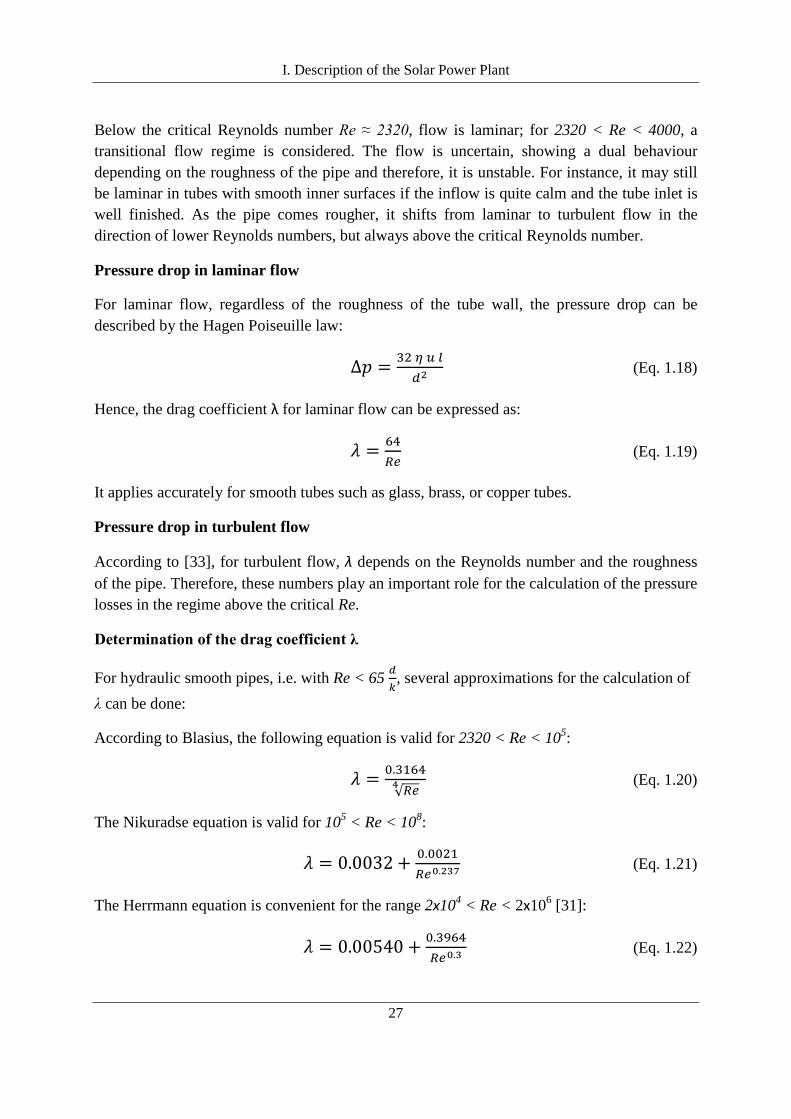
a) For elbows with circular cross-section (Fig. 1.16) [37]: Table 1.5 shows the drag coefficients for smooth and rough pipes with different angles. The drag coefficient assumed was the average of the values corresponding to a 90° angle, that is, 𝜁 = 1.20.


31

Fig. 1.16 Single elbow with circular cross-section

Table 1.5 Drag coefficients for single elbows as a function of the angle δ

δ 22.5° 30° 45° 60° 90°

ζ (smooth) 0.07 0.11 0.24 0.47 1.13

ζ (rough) 0.11 0.17 0.32 0.68 1.27

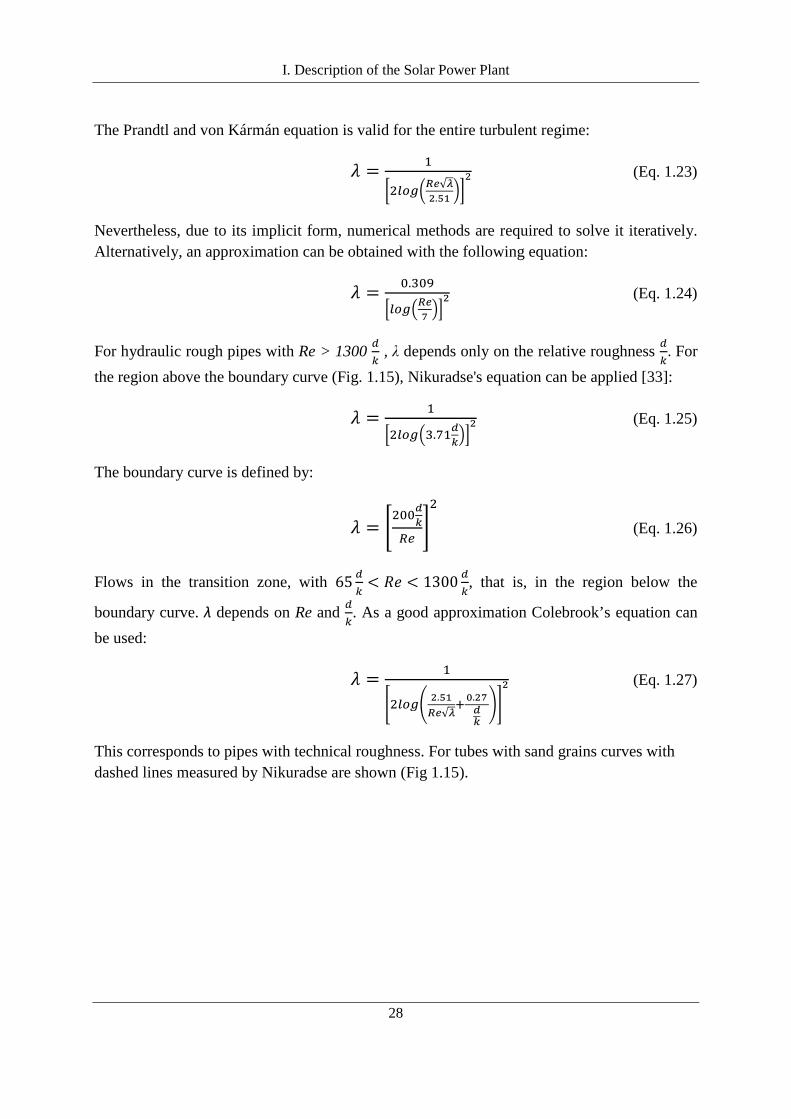
b) For pipe branching and unions [38]: Fig. 1.17 shows different profiles for pipe branching and unions. The corresponding drag coefficients are calculated according to the relation of the inlet and outlet cross sections in the pipes. The drag coefficients are shown in Table 1.6.

Fig. 1.17 Branching and union pipe profiles

�� = 𝑇𝑜𝑡𝑎𝑙 𝑐𝑢𝑟𝑟𝑒𝑛𝑡 𝑉�� = 𝑂𝑢𝑡𝑓𝑙𝑜𝑤𝑖𝑛𝑔 𝑜𝑟 𝐼𝑛𝑓𝑙𝑜𝑤𝑖𝑛𝑔 𝑐𝑢𝑟𝑟𝑒𝑛𝑡 𝜁𝑑 = 𝐷𝑟𝑎𝑔 𝑐𝑜𝑒𝑓𝑓𝑖𝑐𝑖𝑒𝑛𝑡 𝑖𝑛 𝑚𝑎𝑖𝑛 𝑝𝑖𝑝𝑒 𝜁𝑎 = 𝑑𝑟𝑎𝑔 𝑐𝑜𝑒𝑓𝑓𝑖𝑐𝑖𝑒𝑛𝑡 𝑖𝑛 𝑏𝑟𝑎𝑛𝑐ℎ 𝑝𝑖𝑝𝑒


32

Table 1.6 Drag coefficients for pipe branching and pipe unions * Pressure gain indicated with the minus sign

Separation Union Fig.a Fig.b Fig.c Fig.d

𝑽��

𝜻𝒂 𝜻𝒅 𝜻𝒂 𝜻𝒅 𝜻𝒂 𝜻𝒅 𝜻𝒂 𝜻𝒅

0 0.95 0.04 0.9 0.04 −1.2 0.04 −0.92 0.04

0.2 0.88 −0.08 0.68 −0.06 −0.4 0.17 −0.38 0.17

0.4 0.89 −0.05 0.5 −0.04 0.08 0.3 0 0.19

0.6 0.95 0.07 0.38 0.07 0.47 0.41 0.22 0.09

0.8 1.1 0.21 0.35 0.2 0.72 0.51 0.37 −0.17

1 1.28 0.35 0.48 0.33 0.91 0.6 0.37 −0.54

For all the branching a drag coefficient of 𝜁 = 0.35 was selected. Taking the relation 𝑽��

= 1; analogously, for the unions, a drag coefficient of 𝜁 = 0.6 was chosen.

1.5.3 Pressure drop in valves, steam traps, separators and filters The calculation for the hydraulic elements described in section 1.4.2 is shown below. The pressure losses obtained are also shown in Table A2.1.

a) Valves

i) Gate valves: According to [32]

∆𝑃 = 𝐺 � 𝑉𝐾𝑣�2 (Eq. 1.29)

where

Kv = Flow of liquid that will create a pressure drop of 1 bar (m3/h bar)

��= Flow rate (m3/h)

G = Relative density/specific gravity of the liquid (dimensionless)

ΔP = Pressure drop across the valve (bar)

Kv's for different nominal diameters (DN) found in technical data sheets from Spirax Sarco are presented in Table 1.7.


33

Table 1.7 Kv values in gate valves for different nominal diameters

DN Kv

25 12

32 19

50 47

ii) Check valves: Fig 1.18 shows a chart relating the pressure loss in check valves and the water flow rate, 𝑉��. The water flow rate is defined as follows:

𝑉�� = � 𝜌1000

�� (Eq. 1.30)

where

𝑉�� = equivalent water volume flow rate (m3/h)

ρ = density of the liquid (kg/m3)

�� = Volume flow rate of liquid (m3/h)

Once the equivalent water volume flow rate has been determined, the pressure drop across the valve can be read off on the chart. Volumetric flow rate is analogous to mass flow rate and is used typically for liquid applications whereas the mass flow rate is used in steam applications.

Fig. 1.18 Pressure loss diagram for check valves [32]

b) Filters: For pressure losses in filters, Eq. 1.16 is also valid. Kv's for different nominal diameters (DN) found in technical data sheets from Spirax Sarco are presented in Table 1.8.


34

Table 1.8 Kv values in filters for different nominal diameters

DN Kv

25 13

32 22

50 46

The filter assumed for the calculations according to the technical data sheet was a Filter Type 33, DN50.

c) Separator: According to [32], the pressure drop for the separator is relatively low (approximately 0.02 bar).

d) Steam trap: Considering a steam trap Type FT57-4 of the company Spirax Sarco, a corresponding pressure drop of 1 bar was reported in the technical data sheet.

The pressure drop to be handled by the recirculation pump comprises the solar field, steam drum and all equipment between them. Considering also the remaining piping from the steam drum to the feed water pump and the piping from the pump to the solar field, the filter and valves, the total pressure to be compensated by the recirculation pump sums a total of 2.44 bar. The feed water pump will handle the pressure drop related to the piping, valves and other equipment, between the steam drum, the pump and the heat exchangers. For the heat exchangers and control valves associated, a pressure drop of 1 bar was assumed. The total pressure to be compensated by the feed water pump is 2.12 bar, summing thus a total pressure drop in the plant of about 4.6 bar. A breakdown of the pressure drop calculation can be observed in Table A2.1.

In Fig. 1.19, a layout with the elements described along this chapter are shown. Pipes containing water are shown in blue, while pipes in red indicate that the fluid is steam: a water-steam mixture until the steam drum and saturated steam from the steam drum until the heat exchangers. Since the steam temperature at the inlet of the heat exchangers is fixed (175 °C) and the condensate is assumed to be at 80 °C, a backwards calculation is done to describe roughly the parameters along the process using the pressure drops already estimated. The pressure, temperature, mass flow and vapour fraction are shown in crosses at several points of the layout shown in Fig. 1.19. Instrumentation for process measurement is not included in the P&ID, though.


35

Fig. 1.19 Layout of the plant showing the steam lines in red and the condensate and feed water lines in blue

36

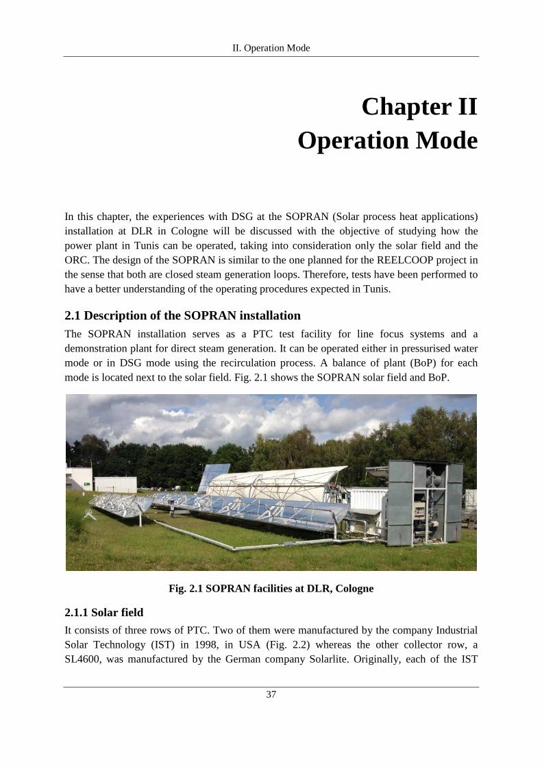
II. Operation Mode

37

Chapter II Operation Mode

In this chapter, the experiences with DSG at the SOPRAN (Solar process heat applications) installation at DLR in Cologne will be discussed with the objective of studying how the power plant in Tunis can be operated, taking into consideration only the solar field and the ORC. The design of the SOPRAN is similar to the one planned for the REELCOOP project in the sense that both are closed steam generation loops. Therefore, tests have been performed to have a better understanding of the operating procedures expected in Tunis.

2.1 Description of the SOPRAN installation The SOPRAN installation serves as a PTC test facility for line focus systems and a demonstration plant for direct steam generation. It can be operated either in pressurised water mode or in DSG mode using the recirculation process. A balance of plant (BoP) for each mode is located next to the solar field. Fig. 2.1 shows the SOPRAN solar field and BoP.

Fig. 2.1 SOPRAN facilities at DLR, Cologne 2.1.1 Solar field It consists of three rows of PTC. Two of them were manufactured by the company Industrial Solar Technology (IST) in 1998, in USA (Fig. 2.2) whereas the other collector row, a SL4600, was manufactured by the German company Solarlite. Originally, each of the IST

II. Operation Mode

38

collectors were composed of 6 modules, however, two modules had been damaged and needed to be removed. The remaining 10 modules sum a net aperture area of about 132 m2.

The collectors use non-evacuated absorber tubes and the tracking system can be done either automatically or manually. The technical specifications of the IST collector modules are shown in Table 2.1.

Fig. 2.2 IST collector at SOPRAN facilities

Table 2.1 Technical specifications of Solitem PTC1800 module at SOPRAN

Technical specifications of IST collector module

Module length 6.1 m

Module width 2.3 m

Aperture area 14.03 m2

Weight approx. 81 kg

Absorber outside diameter 5.08 cm

Medium Water, Steam

Max. operating temperature 200 °C

Reflective Surface aluminized acrylic

The SL4600 collector consists of two modules. Each module has a dimension of 4.6 m aperture width and 12 m length (Fig. 2.3). Nonetheless, due to technical problems with the hydraulics of the tracking system, this collector could not be operated during the test period and it was not included in the tests. Unlike the REELCOOP plant, these collectors have an East-West orientation, which is preferable for testing collectors.

The piping between the outlet of the collectors and the BoP has a sight glass that allows checking qualitatively if a steam flow is being produced.

II. Operation Mode

39

Fig. 2.3 Solarlite SL4600 collector at SOPRAN facilities

2.1.2 Balance of plant In the BoP for DSG mode, the water/steam produced in the solar field is separated in a horizontal steam drum. Since no turbine is used to generate electricity, a condenser acting as a heat exchanger to consume the thermal power produced is used. The condensate mixes with the water recirculated via the downcomer of the steam drum and is sent back to the solar field inlet by a recirculation pump. This allows closed-loop facility operation, thus saving water and energy. The mass flow rate can be regulated by opening a hand valve. The steam drum, condenser, recirculation pump, as well as the associated instrumentation for control and measurement are displayed in Fig. 2.4.

Fig. 2.4 Components of the BoP for DSG: condensing ventilator (top left); steam drum (top right); recirculation pump (bottom centre)

II. Operation Mode

40

The BoP for pressurised water mode was not necessary for the tests done. Nevertheless, the expansion tank within this BoP was required. Due to the changes in the water volume because of the steam generation and temperature differences, as explained in 1.4.2, an expansion tank with 290 L volume was used. The BoP for pressurised water mode and the expansion tank are shown in Fig. 2.5.

Fig. 2.5 Components of the BoP for pressurised water: expansion tank (top).

2.2 Operating procedures of the installation The set-up of the SOPRAN facility served as a previous reference for future tests in the power plant in Tunis in order to facilitate the plant operation by providing a description of the procedure performed to run the installation. The step-by-step process is described below, as well as the considerations taken into account.

Preparations

As a first step when setting-up the system, the collector mirrors and absorber tubes needed to be cleaned. The glass tubes covering the absorber tubes were cleaned softly with demineralized water and a cloth, particularly on the side facing the collector mirrors as the radiation is reflected and concentrated from below. For safety reasons, it was necessary to verify there are no leakages in the system.

To know the parameters of the operation and performance of the plant, it should preferably have a pyrheliometer and a global radiation sensor located next to the installation that operates automatically to measure these parameters. These devices need to be cleaned carefully before being utilised.

To ensure that the system contains no air, a previous deaeration is required. In case air is in the steam drum, it can be observed with the claps position of the level indicator, e.g. after several days and depending on the pressure in the installation (overpressure avoids air

II. Operation Mode

41

intrusion). To deaerate, the recirculation pump is run to circulate the water within the system. The air is then gathered in the upper part of the steam drum. Then the air is dismissed manually by opening a hand valve above the steam drum so that the steam drum is completely full with water. For deaeration, pressure above atmospheric pressure is needed therefore, nitrogen is injected in the expansion tank if the pressure is too low. Concerning the expansion tank, it is necessary not only to guarantee a minimum water level within the tank so that the pressurised nitrogen coming into the tank does not go further into the system but also not to have too much water. To monitor the water level within the expansion tank, as well as in the steam drum, a water level indicator with clap is used. In Fig. 2.6 the expansion tank and the water level are displayed. The red bars (claps) indicate the water level of the expansion tank.

Fig. 2.6 Expansion tank

General Start-up

After the set-up of the plant is ready, the first step is to turn the recirculation pump on. Turning the recirculation pump is essential to avoid damaging the absorber tubes. In case the tracking system of the collectors was started first, the absorber tubes would suffer undesired thermal and mechanical stresses; therefore, it is necessary to ensure water flowing through the absorbers before start focusing the collectors.

After the pump is on, the tracking system of the collectors is started. The mass flow rate is predefined and can be manually corrected. The measurement and control system is started in order to monitor the operation and response of the plant. The collectors need to be focused.

General Shutdown

For a correct shutdown of the plant, it is necessary to turn off the collector tracking system first and then the recirculation pump. Inversely to the step sequence during start-up, in order to avoid mechanical and thermal stresses in the absorber tubes, the very last element to be turned off is the recirculation pump.

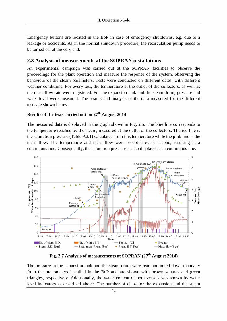
II. Operation Mode

42

Emergency buttons are located in the BoP in case of emergency shutdowns, e.g. due to a leakage or accidents. As in the normal shutdown procedure, the recirculation pump needs to be turned off at the very end.

2.3 Analysis of measurements at the SOPRAN installations An experimental campaign was carried out at the SOPRAN facilities to observe the proceedings for the plant operation and measure the response of the system, observing the behaviour of the steam parameters. Tests were conducted on different dates, with different weather conditions. For every test, the temperature at the outlet of the collectors, as well as the mass flow rate were registered. For the expansion tank and the steam drum, pressure and water level were measured. The results and analysis of the data measured for the different tests are shown below.

Results of the tests carried out on 27th August 2014

The measured data is displayed in the graph shown in Fig. 2.5. The blue line corresponds to the temperature reached by the steam, measured at the outlet of the collectors. The red line is the saturation pressure (Table A2.1) calculated from this temperature while the pink line is the mass flow. The temperature and mass flow were recorded every second, resulting in a continuous line. Consequently, the saturation pressure is also displayed as a continuous line.

Fig. 2.7 Analysis of measurements at SOPRAN (27th August 2014)

The pressure in the expansion tank and the steam drum were read and noted down manually from the manometers installed in the BoP and are shown with brown squares and green triangles, respectively. Additionally, the water content of both vessels was shown by water level indicators as described above. The number of claps for the expansion and the steam

II. Operation Mode

43

drum are displayed as orange and purple column bars in Fig. 2.5 as a qualitative way to know the water content displaced during the process.

The striking facts during the process are marked along the temperature curve with yellow circles, indicating the event occurred at that time. This information allows relating and understanding the behaviour of the system, e.g. during shading by clouds, pump shutdown or defocusing of the collectors. Originally, pressure within the system was about 4.3 bar so pressure was released manually. During the test, several shutdowns of the recirculation pump occurred. The period of time with the pump turned off is shown in grey boxes. After the pressure release was carried out, a shutdown occurred and it was decided to defocus the collectors before restarting the pump. Fig 2.7 shows clearly the abrupt fall of the temperature and mass flow during these periods.

Once steam started being generated, it was gathered in the steam drum, decreasing the water level of the steam drum, meaning a displacement of the water content by the steam produced. Therefore, the number of claps in the steam drum decreased as long as the temperature was rising. On the other hand, the water level of the expansion tank increased because of the water displacement. Steam could also be observed qualitatively through the sight glass at the outlet of the collectors. Since only the IST collectors were utilised for the tests, the steam production was accomplished more slowly in comparison to regular tests using all the collectors. Evaporation cannot take place as long as the pressure is above the saturation pressure. A difference between the pressure measured in the steam drum and the saturation pressure can be noticed in the graph, diminishing as the temperature increases and eventually reaching equilibrium at about 130 °C and a maximum temperature of about 160 °C.

Analogously, as the temperature decreases, the water content of the steam drum should rise again. Nonetheless, according to Fig. 2.7, the water content did not change significantly. This might be explained by the steam drum acting as a buffer. The steam within the steam drum is not condensed as fast as the rest of the steam in the installation, so the water content does not change right after the decrease of the temperature.

Results of the tests carried out on 28th August 2014

For this test, a more stable performance was achieved but due to intermittent clouds, only a temperature slightly above 120 °C was reached. In contrast to the test carried out on the 27.08.2014, in the beginning the pressure was increased by injecting nitrogen and no pressure release was performed during the test. The pressure of the steam drum and expansion tank increased as the temperature increased. In contrast, the water content of the steam drum decreased slightly, meaning that some water displacement took place. On the other hand, the volume of water in the expansion tank increased. Even if steam production is partially accomplished, the water displacement by the changes in density when increasing the temperature causes the water level in the expansion tank to rise. The measurements are shown in Fig. 2.8. For a better viewing, Fig. 2.7 and 2.8 can also be found in the Annex.

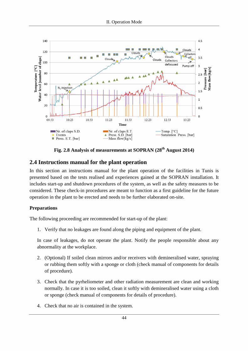
II. Operation Mode

44

Fig. 2.8 Analysis of measurements at SOPRAN (28th August 2014)

2.4 Instructions manual for the plant operation In this section an instructions manual for the plant operation of the facilities in Tunis is presented based on the tests realised and experiences gained at the SOPRAN installation. It includes start-up and shutdown procedures of the system, as well as the safety measures to be considered. These check-in procedures are meant to function as a first guideline for the future operation in the plant to be erected and needs to be further elaborated on-site.

Preparations

The following proceeding are recommended for start-up of the plant:

1. Verify that no leakages are found along the piping and equipment of the plant.

In case of leakages, do not operate the plant. Notify the people responsible about any abnormality at the workplace.

2. (Optional) If soiled clean mirrors and/or receivers with demineralised water, spraying or rubbing them softly with a sponge or cloth (check manual of components for details of procedure).

3. Check that the pyrheliometer and other radiation measurement are clean and working normally. In case it is too soiled, clean it softly with demineralised water using a cloth or sponge (check manual of components for details of procedure).

4. Check that no air is contained in the system.

II. Operation Mode

45

• Check that the steam drum water level indicator is at the top position. If the water level is at the highest position, no air is contained in the system. If the water level is below the highest position, then deaeration is needed.

• For deaeration:

o Make sure the collectors are in off position (not focused).

o Check the pressure of the expansion tank. Pressure above atmospheric pressure is required for deaeration.

o Make sure the pressure in the expansion tank is about 2 bar (absolute pressure). In case of lower pressure, inject nitrogen by opening manually the nitrogen tank hand valve until reaching a pressure of about 2 bar in the expansion tank. In case of higher pressure, release nitrogen into the atmosphere by opening the exhaust valve of the expansion tank until the pressure reaches 2 bar.

o When cold and with a pressure of 2 bar, make sure that the minimum water level in the expansion tank is about 100 L.

o Run the recirculation pump. Air contained in the system will then be gathered in the upper part of the steam drum.

o Open carefully the hand valve connected to the upper part of the steam drum in order to release the air contained there.

o Once only water starts coming out from the valve, close the hand valve manually.

5. Check that the measurement instrumentation and monitoring equipment are working normally e.g. thermistors, manometers, flow meters, water level indicators, etc. In case of any failure, please notify the people responsible.

Start-up

Once the points above are ready, the start-up of the plant can be done following the steps below:

1. Make sure the collectors are in off position.

2. Turn the recirculation pump on.

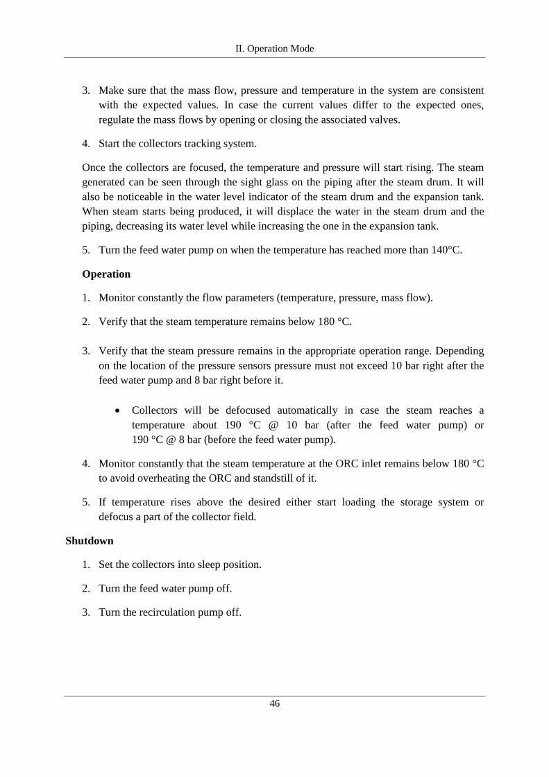
II. Operation Mode

46

3. Make sure that the mass flow, pressure and temperature in the system are consistent with the expected values. In case the current values differ to the expected ones, regulate the mass flows by opening or closing the associated valves.

4. Start the collectors tracking system.

Once the collectors are focused, the temperature and pressure will start rising. The steam generated can be seen through the sight glass on the piping after the steam drum. It will also be noticeable in the water level indicator of the steam drum and the expansion tank. When steam starts being produced, it will displace the water in the steam drum and the piping, decreasing its water level while increasing the one in the expansion tank.

5. Turn the feed water pump on when the temperature has reached more than 140°C.

Operation

1. Monitor constantly the flow parameters (temperature, pressure, mass flow).

2. Verify that the steam temperature remains below 180 °C.

3. Verify that the steam pressure remains in the appropriate operation range. Depending on the location of the pressure sensors pressure must not exceed 10 bar right after the feed water pump and 8 bar right before it.

• Collectors will be defocused automatically in case the steam reaches a temperature about 190 °C @ 10 bar (after the feed water pump) or 190 °C @ 8 bar (before the feed water pump).

4. Monitor constantly that the steam temperature at the ORC inlet remains below 180 °C to avoid overheating the ORC and standstill of it.

5. If temperature rises above the desired either start loading the storage system or defocus a part of the collector field.

Shutdown

1. Set the collectors into sleep position.

2. Turn the feed water pump off.

3. Turn the recirculation pump off.

IV. Conclusions

47

Chapter III Calculation of Electricity Generation

According to the dimensioning of the piping system and vessels carried out in previous chapters, as well as the technical specifications of the collectors and the ORC, the performance of the solar field and the ORC in nominal and partial load are determined using the software Greenius. Based on these software results and meteorological data from the site, the gross annual electricity generation is calculated. This calculation may serve as a reference for future simulations and may be improved once the erection of the plant takes place. Since some prototype developments within the plant design are ongoing, the simulations presented here consider only the solar field and the ORC.

3.1 Solar field efficiency The solar field efficiency can be calculated by empirical formulas. These formulas depend on two main factors: the optical and thermal efficiencies. The optical efficiency is affected by optical properties of the reflecting surface, transmission losses at the glass envelope tube, receiver absorption losses and the intercept factor. The intercept factor involves the losses caused by reflected rays missing the receiver tube due to imperfections of the collector components. The thermal efficiencies are related to the heat losses e.g. due to the radiative and convective heat losses at the receiver.

The incidence angle modifier (IAM) expresses the dependence of the optical efficiency 𝜂0 as a function of the position of the sun. For one-axis tracked systems, the IAM depends on 𝜃, the angle between the sun and the tracked plane. To calculate the efficiency of the collector the following empirical formulas are used by Greenius:

𝐼𝐴𝑀 = 1 − 𝑎1∙𝜃+𝑎2∙𝜃2+𝑎3∙𝜃3

𝑐𝑜𝑠𝜃 (Eq. 3.1)

𝐾 = 𝐼𝐴𝑀 ∙ 𝑐𝑜𝑠𝜃 (Eq. 3.2)

𝜂𝑐𝑜𝑙𝑙𝑒𝑐𝑡𝑜𝑟𝑠 = 𝐾 ∙ 𝜂0 − �𝐾 ∙ 𝑏0 ∙ ∆𝑇 + 𝑏1∆𝑇+𝑏2∆𝑇2+𝑏3∆𝑇3+𝑏4∆𝑇4

𝐷𝑁𝐼� (Eq. 3.3)

∆𝑇 is the temperature difference between the mean collector temperature and the ambient temperature.

∆𝑇 = 𝑇𝑖𝑛+𝑇𝑜𝑢𝑡2

− 𝑇𝑎𝑚𝑏 (Eq. 3.4)

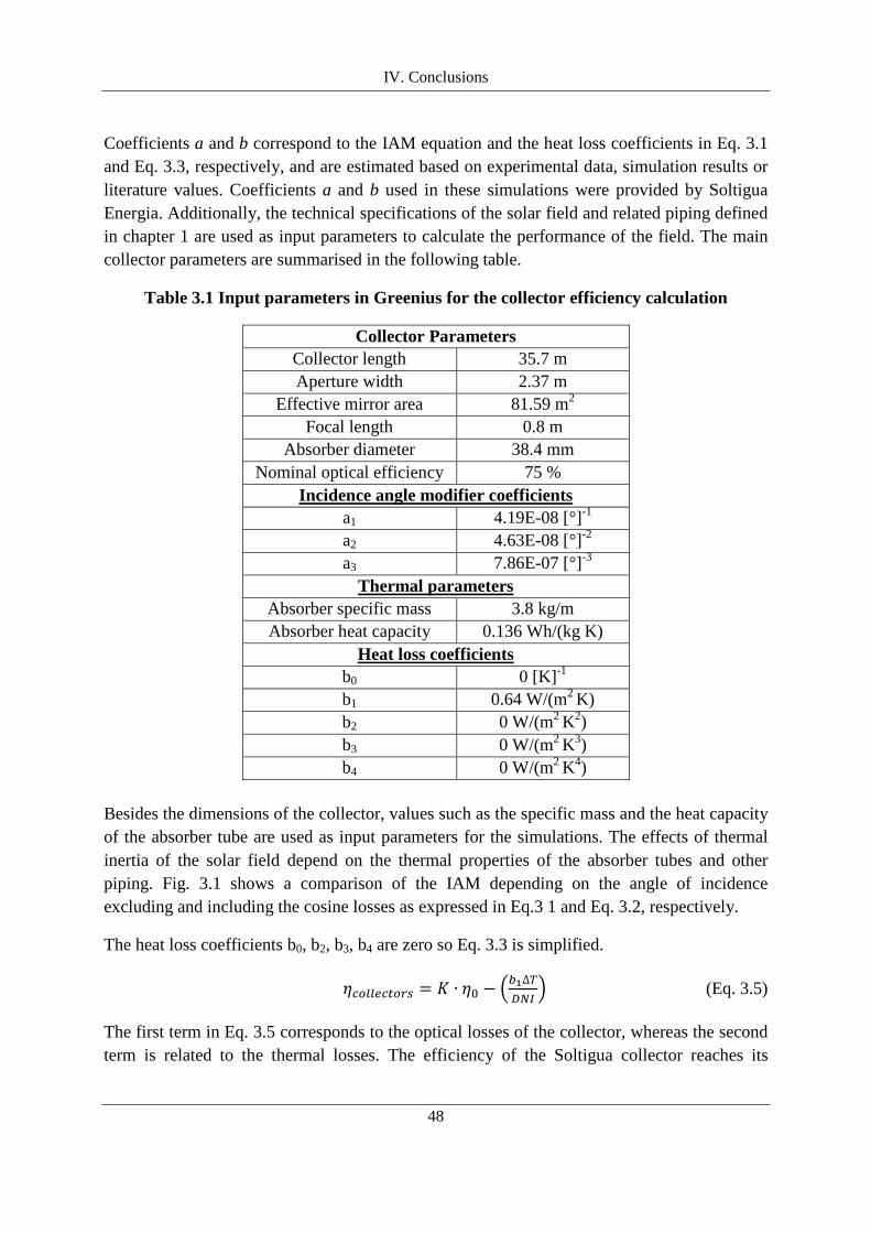
IV. Conclusions

48

Coefficients a and b correspond to the IAM equation and the heat loss coefficients in Eq. 3.1 and Eq. 3.3, respectively, and are estimated based on experimental data, simulation results or literature values. Coefficients a and b used in these simulations were provided by Soltigua Energia. Additionally, the technical specifications of the solar field and related piping defined in chapter 1 are used as input parameters to calculate the performance of the field. The main collector parameters are summarised in the following table.

Table 3.1 Input parameters in Greenius for the collector efficiency calculation

Collector Parameters Collector length 35.7 m Aperture width 2.37 m

Effective mirror area 81.59 m2 Focal length 0.8 m

Absorber diameter 38.4 mm Nominal optical efficiency 75 %

Incidence angle modifier coefficients a1 4.19E-08 [°]-1

a2 4.63E-08 [°]-2 a3 7.86E-07 [°]-3

Thermal parameters Absorber specific mass 3.8 kg/m Absorber heat capacity 0.136 Wh/(kg K)

Heat loss coefficients b0 0 [K]-1 b1 0.64 W/(m2 K)

b2 0 W/(m2 K2) b3 0 W/(m2 K3) b4 0 W/(m2 K4)

Besides the dimensions of the collector, values such as the specific mass and the heat capacity of the absorber tube are used as input parameters for the simulations. The effects of thermal inertia of the solar field depend on the thermal properties of the absorber tubes and other piping. Fig. 3.1 shows a comparison of the IAM depending on the angle of incidence excluding and including the cosine losses as expressed in Eq.3 1 and Eq. 3.2, respectively.

The heat loss coefficients b0, b2, b3, b4 are zero so Eq. 3.3 is simplified.

𝜂𝑐𝑜𝑙𝑙𝑒𝑐𝑡𝑜𝑟𝑠 = 𝐾 ∙ 𝜂0 − �𝑏1∆𝑇𝐷𝑁𝐼

� (Eq. 3.5)

The first term in Eq. 3.5 corresponds to the optical losses of the collector, whereas the second term is related to the thermal losses. The efficiency of the Soltigua collector reaches its

IV. Conclusions

49

maximum when θ is zero and decreases when the solar beam incidence angle increases. On the other hand, the thermal losses are diminished as the DNI increases.

Fig. 3.1 IAM depending on the angle of incidence θ: excluding cosine losses (left); including cosine losses (right)

The collector absorbs more energy along with solar insolation increasing. Although the thermal losses also increment due to the increased collector temperature, it is smaller than the enhanced absorbed solar energy [39]. A comparison of the collector efficiency for different values of DNI is displayed in Fig. 3.2.

Fig. 3.2 Collector efficiency for different DNI

For nominal operation, a DNI of 800 W/m2 is considered. The outlet and inlet temperatures of the collector at nominal operation are about 175 °C and 148 °C. Due to evaporation at nearly constant temperature, the mean collector temperature is not the arithmetic mean between inlet and outlet temperature. Instead, Greenius calculates a mean collector temperature of 175.4 °C,

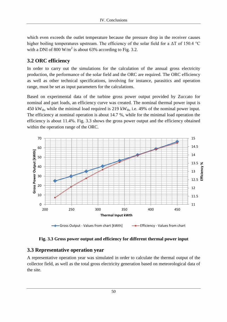
IV. Conclusions

50

which even exceeds the outlet temperature because the pressure drop in the receiver causes higher boiling temperatures upstream. The efficiency of the solar field for a ΔT of 150.4 °C with a DNI of 800 W/m2 is about 63% according to Fig. 3.2.

3.2 ORC efficiency In order to carry out the simulations for the calculation of the annual gross electricity production, the performance of the solar field and the ORC are required. The ORC efficiency as well as other technical specifications, involving for instance, parasitics and operation range, must be set as input parameters for the calculations.

Based on experimental data of the turbine gross power output provided by Zuccato for nominal and part loads, an efficiency curve was created. The nominal thermal power input is 450 kWth, while the minimal load required is 219 kWth, i.e. 49% of the nominal power input. The efficiency at nominal operation is about 14.7 %, while for the minimal load operation the efficiency is about 11.4%. Fig. 3.3 shows the gross power output and the efficiency obtained within the operation range of the ORC.

Fig. 3.3 Gross power output and efficiency for different thermal power input

3.3 Representative operation year A representative operation year was simulated in order to calculate the thermal output of the collector field, as well as the total gross electricity generation based on meteorological data of the site.

11

11.5

12

12.5

13

13.5

14

14.5

15

0

10

20

30

40

50

60

70

200 250 300 350 400 450

Effic

ienc

y %

Gro

ss P

ower

Out

put [

kWth

]

Thermal Input kWth

Gross Output - Values from chart [kWth] Efficiency - Values from chart

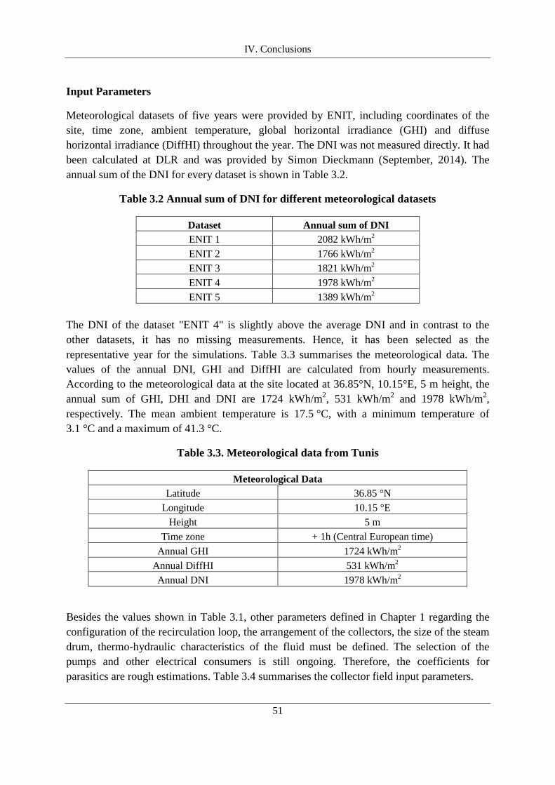
IV. Conclusions

51

Input Parameters

Meteorological datasets of five years were provided by ENIT, including coordinates of the site, time zone, ambient temperature, global horizontal irradiance (GHI) and diffuse horizontal irradiance (DiffHI) throughout the year. The DNI was not measured directly. It had been calculated at DLR and was provided by Simon Dieckmann (September, 2014). The annual sum of the DNI for every dataset is shown in Table 3.2.

Table 3.2 Annual sum of DNI for different meteorological datasets

Dataset Annual sum of DNI ENIT 1 2082 kWh/m2

ENIT 2 1766 kWh/m2 ENIT 3 1821 kWh/m2 ENIT 4 1978 kWh/m2 ENIT 5 1389 kWh/m2

The DNI of the dataset "ENIT 4" is slightly above the average DNI and in contrast to the other datasets, it has no missing measurements. Hence, it has been selected as the representative year for the simulations. Table 3.3 summarises the meteorological data. The values of the annual DNI, GHI and DiffHI are calculated from hourly measurements. According to the meteorological data at the site located at 36.85°N, 10.15°E, 5 m height, the annual sum of GHI, DHI and DNI are 1724 kWh/m2, 531 kWh/m2 and 1978 kWh/m2, respectively. The mean ambient temperature is 17.5 °C, with a minimum temperature of 3.1 °C and a maximum of 41.3 °C.

Table 3.3. Meteorological data from Tunis

Meteorological Data Latitude 36.85 °N

Longitude 10.15 °E Height 5 m

Time zone + 1h (Central European time) Annual GHI 1724 kWh/m2

Annual DiffHI 531 kWh/m2 Annual DNI 1978 kWh/m2

Besides the values shown in Table 3.1, other parameters defined in Chapter 1 regarding the configuration of the recirculation loop, the arrangement of the collectors, the size of the steam drum, thermo-hydraulic characteristics of the fluid must be defined. The selection of the pumps and other electrical consumers is still ongoing. Therefore, the coefficients for parasitics are rough estimations. Table 3.4 summarises the collector field input parameters.

IV. Conclusions

52

Table 3.4 Collector field input parameters

Collector Field Parameters Reference Irradiation 800 W/m2 Nominal Thermal Output 449 kWth Distance between rows 7.20 m Distance between collectors 1 m Number of rows in the field 3 Number of collectors/row (loop) 4 Field size (effective mirror area) 979 m2 Total header length 130 m Pipe length in loops 30 m Pipe diameter in loops 0.0409 m Pipe specific mass 4.05 kg/m Drum length 0.5 m Drum diameter 0.7 m Drum specific mass 550 kg/m Recirculation rate 3.6 Heat capacity 0.136 Wh/(kg K) Nominal field outlet temperature 175 °C Nominal field inlet temperature 148 °C

Parasitic modifiers Constant need 1 W/m2 SF Power of field pump 0.5 W/m2 SF

Pipes Piping loss coefficient 0.145 W/(m2 K) Expansion vessel losses 0.0330 W/(m2 K)

Mass flow Nominal fluid mass flow rate 0.184 kg/s Nominal field outlet pressure 9 bar Nominal pressure drop of the solar field 2.4 bar

As mentioned above, the power block is defined as an input parameter for this simulation. The performance is stored in a separate lookup table. The lookup table was elaborated from technical specifications of the ORC provided by the company Zuccato, previous calculations at DLR and assumptions based on PTC power plants with similar characteristics in regard to the dimensions and power range. Table 3.5 shows a summary of the data stored in the lookup table used for the power block modelling.

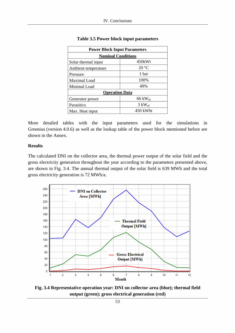
IV. Conclusions

53

Table 3.5 Power block input parameters

Power Block Input Parameters Nominal Conditions

Solar thermal input 450kWt Ambient temperature 20 °C Pressure 1 bar Maximal Load 100% Minimal Load 49%

Operation Data Generator power 66 kWel Parasitics 3 kWel Max. Heat input 450 kWht

More detailed tables with the input parameters used for the simulations in Greenius (version 4.0.6) as well as the lookup table of the power block mentioned before are shown in the Annex.

Results

The calculated DNI on the collector area, the thermal power output of the solar field and the gross electricity generation throughout the year according to the parameters presented above, are shown in Fig. 3.4. The annual thermal output of the solar field is 639 MWh and the total gross electricity generation is 72 MWh/a.

Fig. 3.4 Representative operation year: DNI on collector area (blue); thermal field

output (green); gross electrical generation (red)

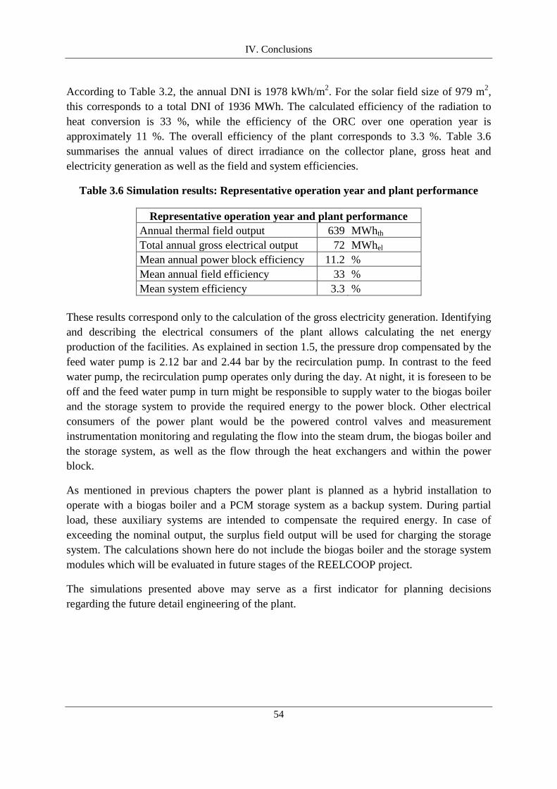
IV. Conclusions

54

According to Table 3.2, the annual DNI is 1978 kWh/m2. For the solar field size of 979 m2, this corresponds to a total DNI of 1936 MWh. The calculated efficiency of the radiation to heat conversion is 33 %, while the efficiency of the ORC over one operation year is approximately 11 %. The overall efficiency of the plant corresponds to 3.3 %. Table 3.6 summarises the annual values of direct irradiance on the collector plane, gross heat and electricity generation as well as the field and system efficiencies.

Table 3.6 Simulation results: Representative operation year and plant performance

Representative operation year and plant performance Annual thermal field output 639 MWhth Total annual gross electrical output 72 MWhel Mean annual power block efficiency 11.2 % Mean annual field efficiency 33 % Mean system efficiency 3.3 %

These results correspond only to the calculation of the gross electricity generation. Identifying and describing the electrical consumers of the plant allows calculating the net energy production of the facilities. As explained in section 1.5, the pressure drop compensated by the feed water pump is 2.12 bar and 2.44 bar by the recirculation pump. In contrast to the feed water pump, the recirculation pump operates only during the day. At night, it is foreseen to be off and the feed water pump in turn might be responsible to supply water to the biogas boiler and the storage system to provide the required energy to the power block. Other electrical consumers of the power plant would be the powered control valves and measurement instrumentation monitoring and regulating the flow into the steam drum, the biogas boiler and the storage system, as well as the flow through the heat exchangers and within the power block.

As mentioned in previous chapters the power plant is planned as a hybrid installation to operate with a biogas boiler and a PCM storage system as a backup system. During partial load, these auxiliary systems are intended to compensate the required energy. In case of exceeding the nominal output, the surplus field output will be used for charging the storage system. The calculations shown here do not include the biogas boiler and the storage system modules which will be evaluated in future stages of the REELCOOP project.

The simulations presented above may serve as a first indicator for planning decisions regarding the future detail engineering of the plant.

IV. Conclusions

55

Chapter IV Conclusions

This thesis is part of the REELCOOP project and seeks to contribute in the pre-design phase of a concentrating solar power plant to be erected in Tunis. The complete plant comprises a PTC field with DSG and an ORC as well as a biomass boiler and a PCM storage system. The construction of this plant has educational purposes and will demonstrate the integration of different technologies.

The first chapter contains an overview of the different technologies that will integrate the power plant. The elaboration of different layouts of the plant as well as the definition of the instrumentation and the dimensioning of the piping system, the expansion tank and the steam drum were carried out. The dimensioning was done based on the characteristic flow velocities for water- and steam flows, as well as on the standard commercial diameters and the pressure drops along the process. The dimensioning of the expansion tank has taken into account all the water volume difference between nominal operation (175 °C @ 8.9 bar) and during the night (20 °C @ 2 bar). A steam drum volume of 200 L and an expansion tank volume of 970 L were determined.

For the selection of the pumps, the calculation of the pressure drop along the system was necessary. A literature review was reported concerning the calculation of the pressure losses for piping, bendings, valves, filters, etc. for water- and steam- single-phase flows. The total pressures calculated to be compensated by the recirculation pump and the feed water pump were 2.44 bar and 2.12 bar, respectively.

The objective of the experimental campaign carried out at SOPRAN test facility in DLR described in the second chapter was to have a better understanding of the operation procedures of a DSG plant. Steam generation and the behaviour of the steam parameters have been tested qualitatively. The experiences obtained during the tests allowed identifying key operation issues, such as deaeration, pressurisation and depressurisation, among others. Based on the results of these experiences, a draft of an instructions manual regarding the preparation, set-up, operation and shutdown of the plant to be erected in Tunis has been elaborated.

The performance of the solar field and ORC for nominal and partial loads was determined with the software Greenius based on the effects of solar intensity and incidence angle, collector dimensions, fluid properties, ambient conditions, operating conditions, measured data of the components provided by the suppliers, among others.

IV. Conclusions

56

The ORC nominal load corresponds to 450 kWth and the minimal load to 219 kWth. According to data provided by Zuccato and scaling of the turbine parameters, an efficiency equal to 14.7 % was found at nominal operation while for a minimal load operation the efficiency calculated was 11.4 %. A small amount of the waste heat from the power block is used to enhance the biogas reactor nonetheless; most of the waste heat is not exploited due to its low energy range. For economical reasons, a higher utilisation of the waste heat is recommended. To that end, it is necessary to run the ORC at higher outlet temperatures, so that an industrial consumer or cooling machine can be supplied. This is foreseen as an outlook of the technology for future stages.

Based on meteorological data from the site, the annual electricity generation for a representative operation year was calculated using the software Greenius. For these simulations only the solar field and the ORC were taken into consideration. Due to the lack of technical specifications from several electrical consumers, such as the pumps, these were not included in this calculation. For an annual DNI of 1978 kWh/m2, the annual thermal output of the solar field is 639 MWh and the total gross electricity generation is 72 MWh/a. The calculated efficiency of the radiation to heat conversion is 33 %, while the efficiency of the ORC over one operation year is approximately 11 %. The overall efficiency of the plant corresponds to 3.3 %.

This thesis contains not only the work carried out at DLR but it also compiles a brief overview of the research from other colleagues and partner institutions working within the REELCOOP project and is part of the detailed engineering for the power plant erection in 2015.

Annex

57

Fig. A1.1 Top view layout of the plant.

Condensate piping in blue, steam piping in red

Annex Annex

57

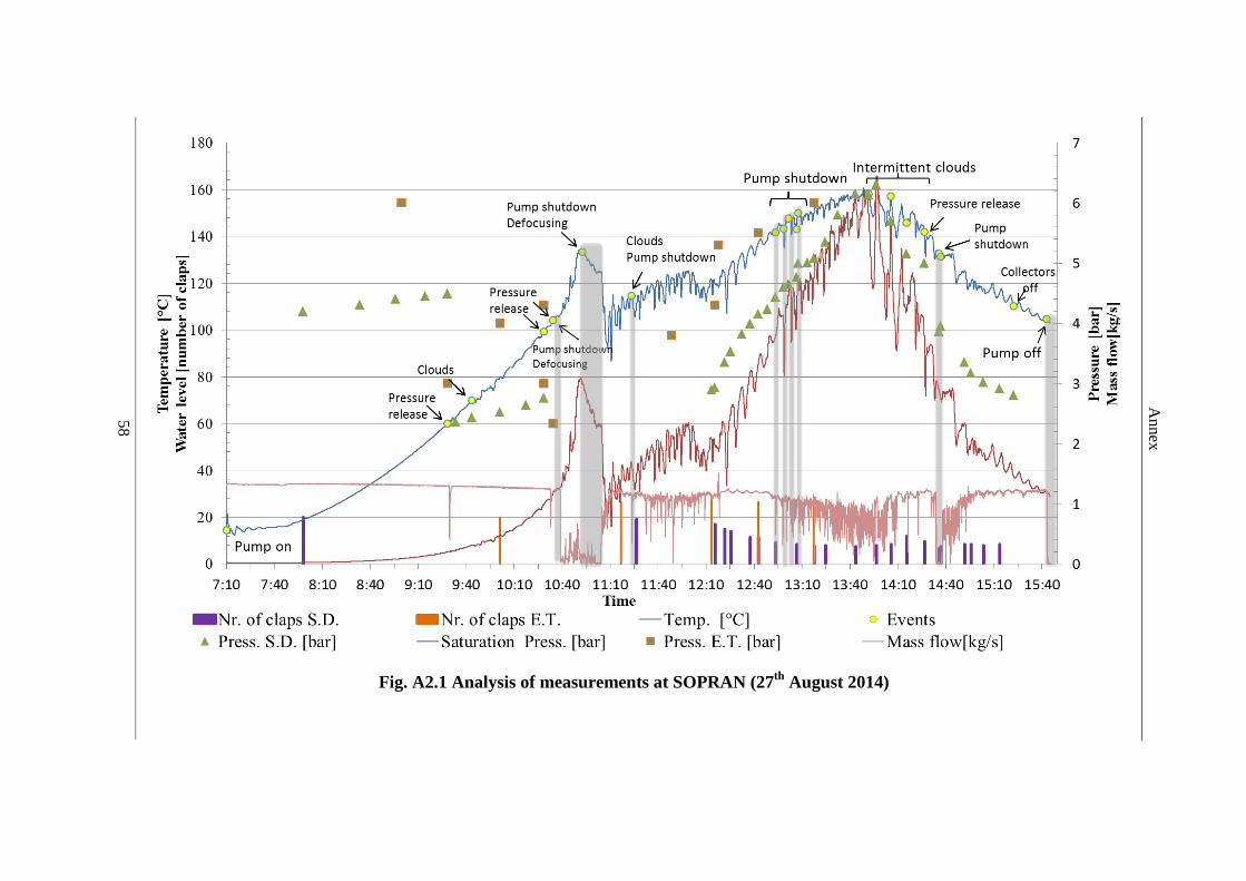
Annex

58

Fig. A2.1 Analysis of measurements at SOPRAN (27th August 2014)

58

Annex

Annex

59

Fig. A2.2 Analysis of measurements at SOPRAN (28th August 2014)

59

Annex

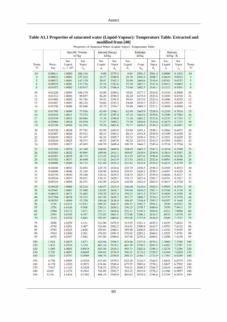
Annex

60

Table A1.1 Properties of saturated water (Liquid-Vapour): Temperature Table. Extracted and modified from [40]

Annex

61

Table A1.2 Physical characteristics of water: Temperature Table. Extracted and modified from [41]

Physical Characteristics of Water: Temperature table

Temp. Pressure Density Specific heat

Dynamic viscosity μ x 106

Kinematic viscosity ν x 106 Temp.

[°C] [bar] [kg/m3] [kJ/kgK] [Pas] [m2/s] [°C] 0 1.013 999.9 4.212 1788 1.789 0

10 1.013 999.7 4.191 1306 1.306 10 20 1.013 998.2 4.183 1004 1.006 20 30 1.013 995.7 4.174 801.5 0.805 30 40 1.013 992.2 4.174 653.3 0.659 40 50 1.013 988.1 4.174 549.4 0.556 50 60 1.013 983.1 4.179 469.9 0.478 60 70 1.013 977.8 4.187 406.1 0.415 70 80 1.013 971.8 4.195 355.1 0.365 80 90 1.013 965.3 4.208 314.9 0.326 90 100 1.013 958.4 4.22 282.5 0.295 100 110 1.43 951 4.233 259 0.272 110 120 1.98 943.1 4.25 237.4 0.252 120 130 2.7 934.8 4.266 217.8 0.233 130 140 3.61 926.1 4.287 201.1 0.217 140 150 4.76 917 4.313 186.4 0.203 150 160 6.18 907.4 4.346 173.6 0.191 160 170 7.92 897.3 4.38 162.8 0.181 170 180 10.03 886.9 4.417 153 0.173 180 190 12.55 876 4.459 144.2 0.165 190 200 15.55 863 4.505 136.4 0.158 200

Annex

62

CALCULATION OF PRESSURE DROPS

Component 2-B Feedwater Pump - Union with recirculation from Steam Drum B-3 Union from Steam Drum - Recirculation Pump

Type of component Pipe Check Valve Valve Branch 1 (A) Branch 2 (13) Branch 3 (B) Pipe Elbow Valve Filter

Type of Fluid Water Water Water Water Water Water Water Water Water Water

Pressure [bar] 8 8 8 8 8 8 8 8 8 8

Temperature [°C] 80 80 80 80 80 170 148 148 148 148

Mass Flow [kg/s] 0.177 0.177 0.177 0.177 0.177 0.473 0.650 0.650 0.650 0.650

Volume flow [m3/h] 0.655 0.655 0.655 0.655 0.655 1.897 2.546 2.546 2.546 2.546

Length [m] 4.50 - - - - - 0.50 - - -

Diameter [mm] 27.2 27.2 27.2 27.2 27.2 27.2 53.0 53.0 53.0 53.0

Drag coefficient - - - 0.35 0.35 0.6 - 1.20 - -

Kvs - values - - 12 - - - - - 47 46

Density [Kg/m3] 972.12 972.12 972.12 972.12 972.12 897.46 919.06 919.06 919.06 919.06 Velocity [m/s] 0.31 0.31 0.31 0.31 0.31 0.91 0.32 0.32 0.32 0.32

Dyn. Viscosity [Pa*s] 3.55E-04 - - - - - 1.85E-04 - - -

Roughness k [mm] 0.020 - - - - - 0.020 - - -

d/k 1360.00 - - - - - 2650 - - -

Reynolds Nr 23369.63 - - - - - 84313 - - -

Lambda 0.0182 - - - - - 0.0157 - - -

Pressure loss [Pa] 143.96 2000 290 17 17 221 7.0 57 270 282

Pressure Loss [bar] 0.00144 0.02 0.003 0.0002 0.0002 0.002 0.0001 0.001 0.003 0.003

Table A2.1 (Continued) Calculation of Pressure Drops (Part 1)

Annex

62

Annex

63


Component 4-5 Recirculation pump - Separation of pipes going to the

solar collectors 5-6 Separation of pipes going to the solar collectors - Input of Solar collectors

Type of component Pipe Pipe

Check Valve Valve Elbow 1 Elbow 2

T junction Pipe

Elbow 1

Valve 1 Branch

Valve 2

Elbow 2

Valve 3

Type of Fluid Water Water Water Water Water Water Water Water Water Water Water Water Water Water

Pressure [bar] 8 8.7 8.7 8.7 8.7 8.7 8.7 8.7 8.7 8.7 8.7 8.7 8.7 8.7

Temperature [°C] 80 148 148 148 148 148 148 148 148 148 148 148 148 148

Mass Flow [kg/s] 0.177 0.650 0.650 0.650 0.650 0.650 0.650 0.217 0.217 0.217 0.217 0.217 0.217 0.217 Volume flow

[m3/h] 0.655 2.546 2.546 2.546 2.546 2.546 2.546 0.849 0.849 0.849 0.849 0.849 0.849 0.849

Length [m] 4.50 8.00 - - - - - 31.80 - - - - - -

Diameter [mm] 27.2 53.0 53.0 53.0 53.0 53.0 53.0 53.0 53.0 53.0 53.0 53.0 53.0 53.0

Drag coefficient - - - - 1.20 1.20 1.20 - 1.20 - 0.35 - 1.20 -

Kvs - values - - - 47 - - ? - - 47 0.015 47 - 47

Density [Kg/m3] 972.12 919.10 919.10 919.10 919.10 919.10 919.10 919.10 919.10 919.10 919.10 919.10 919.10 919.10

Velocity [m/s] 0.31 0.32 0.32 0.32 0.32 0.32 0.32 0.11 0.11 0.11 0.11 0.11 0.11 0.11 Dyn. Viscosity

[Pa*s] 3.55E-04 1.85E-04 - - - - - 1.85E-04 - - - - - -

Roughness k [mm] 0.020 0.020 - - - - - 0.020 - - - - - -

d/k 1360.00 2650 - - - - - 2650 - - - - - -

Reynolds Nr 23369.63 84305 - - - - - 28102 - - - - - -

Lambda 0.0182 0.0157 - - - - - 0.0157 - - - - - -

z 143.96 112 2500 270 57 57 57 16 6 60000 2 60000 6 60000 Pressure Loss

[bar] 0.00144 0.001 0.03 0.003 0.001 0.001 0.001 0.000 0.000 0.60 0.0000 0.60 0.000 0.60


Annex

63

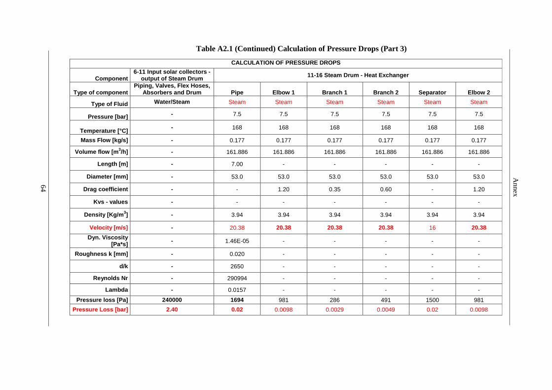
Annex

64


Component 6-11 Input solar collectors -

output of Steam Drum 11-16 Steam Drum - Heat Exchanger

Type of component Piping, Valves, Flex Hoses,

Absorbers and Drum Pipe Elbow 1 Branch 1 Branch 2 Separator Elbow 2

Type of Fluid Water/Steam Steam Steam Steam Steam Steam Steam

Pressure [bar] - 7.5 7.5 7.5 7.5 7.5 7.5

Temperature [°C] - 168 168 168 168 168 168

Mass Flow [kg/s] - 0.177 0.177 0.177 0.177 0.177 0.177

Volume flow [m3/h] - 161.886 161.886 161.886 161.886 161.886 161.886

Length [m] - 7.00 - - - - -

Diameter [mm] - 53.0 53.0 53.0 53.0 53.0 53.0

Drag coefficient - - 1.20 0.35 0.60 - 1.20

Kvs - values - - - - - - -

Density [Kg/m3] - 3.94 3.94 3.94 3.94 3.94 3.94

Velocity [m/s] - 20.38 20.38 20.38 20.38 16 20.38 Dyn. Viscosity

[Pa*s] - 1.46E-05 - - - - -

Roughness k [mm] - 0.020 - - - - -

d/k - 2650 - - - - -

Reynolds Nr - 290994 - - - - -

Lambda - 0.0157 - - - - -

Pressure loss [Pa] 240000 1694 981 286 491 1500 981 Pressure Loss [bar] 2.40 0.02 0.0098 0.0029 0.0049 0.02 0.0098


Annex

64

Annex

65


Component 16-17 ORC components 17-1 HEX - Feed Water Pump Type of

component Control Valve

ORC H Ex 1 H Ex 2 Pipe Elbow 1,2,3 Steam Trap Branch 1 Elbow 4 Branch 2 Elbow 5 Valve Filter

Type of Fluid - - - Water Water Water Water Water Water Water Water Water

Pressure [bar] - - - 6 6 6 6 6 6 6 6 6

Temperature [°C] - - - 80 80 80 80 80 80 80 80 80

Mass Flow [kg/s] - - - 0.177 0.177 0.177 0.177 0.177 0.177 0.177 0.177 0.177

Volume flow [m3/h] - - - 0.656 0.656 0.656 0.656 0.656 0.656 0.656 0.656 0.656

Length [m] - - - 4.50 - - - - - - - -

Diameter [mm] - - - 27.2 27.2 27.2 27.2 27.2 27.2 27.2 27.2 27.2

Drag coefficient - - - - 1.20 - 0.60 1.20 0.60 1.20 - -

Kvs - values - - - - - - - - - - 12 13

Density [Kg/m3] - - - 972.03 972.03 972.03 972.03 972.03 972.03 972.03 972.03 972.03

Velocity [m/s] - - - 0.31 0.31 0.31 0.31 0.31 0.31 0.31 0.31 0.31 Dyn. Viscosity

[Pa*s] - - - 3.54E-04 - - - - - - - -

Roughness k [mm] - - - 0.020 - - - - - - - -

d/k - - - 1360 - - - - - - - -

Reynolds Nr - - - 23373 - - - - - - - -

Lambda - - - 0.0182 - - - - - - - -

Pressure loss [Pa] 100000 144 57 100000 29 57 1500 57 290.1 247.2 Pressure Loss

[bar] 1 0.0014 0.001 1.00 0.015 0.001 0.015 0.001 0.003 0.002



Annex

65

Annex

66

Table A3.1 Input parameters in Greenius for the collector efficiency calculation

Collector Assembly Input Parameters Simple assembly characteristics

Collector´s name Soltigua PTMx-hp-36 Collector type Trough

Collector length 35.7 m Aperture width 2.37 m

Effective mirror area 81.59 m2 Focal length 0.8 m

Absorber diameter 0.0384 m Nominal optical efficiency 75%

Incidence angle modifier a1 4.19E-08 [°]-1

a2 4.63E-08 [°]-2

a3 7.86E-07 [°]-3 Thermal parameters

Absorber specific mass 3.8 kg/m Absorber heat capacity 0.136 Wh/(kg K)

Heat loss coefficients b0 0 [K]-1

b1 0.64 W/(m2 K)

b2 0 W/(m2 K2)

b3 0 W/(m2 K3)

b4 0 W/(m2 K4)

Table A3.2 Collector field input parameters in Greenius (physical properties of water)

Density [kg/m3]

Heat capacity [Wh/(kg K)]

Temperature [°C]

1007 1.146 20 816 1.3 250 601 2.245 350

Annex

67

Table A3.3 Collector field input parameters (field data)

Collector Field Input Parameters Field Data

General Enhanced field model Field type: Evaporator Name REELCOOP Collector Name Soltigua PTMx-hp-36 Land use 3240 m2 Reference Irradiation 800 W/m2 Nominal Thermal Output 449 kWth

Orientation Distance between rows 7.20 m Distance between collectors 1 m Tracking axis tilt angle 0 °C Tracking axis azimuth 0 °C End gain possible Yes

Field parameters Number of rows in the field 3 Number of collectors/row (loop) 4 Field size (effective mirror area) 979 m2 Total head length 130 m Mean header diameter 0.0525 m Header specific mass 5.44 kg/m Length fraction cold header 1 Pipe length in loops 30 m Pipe diameter in loops 0.0409 m Pipe specific mass 4.05 kg/m Drum length 0.5 m Drum diameter 0.7m Drum specific mass 550 kg/m Recirculation rate 3.6 Heat capacity 0.136 Wh/(kg K) Automatic calculation of pipe length No

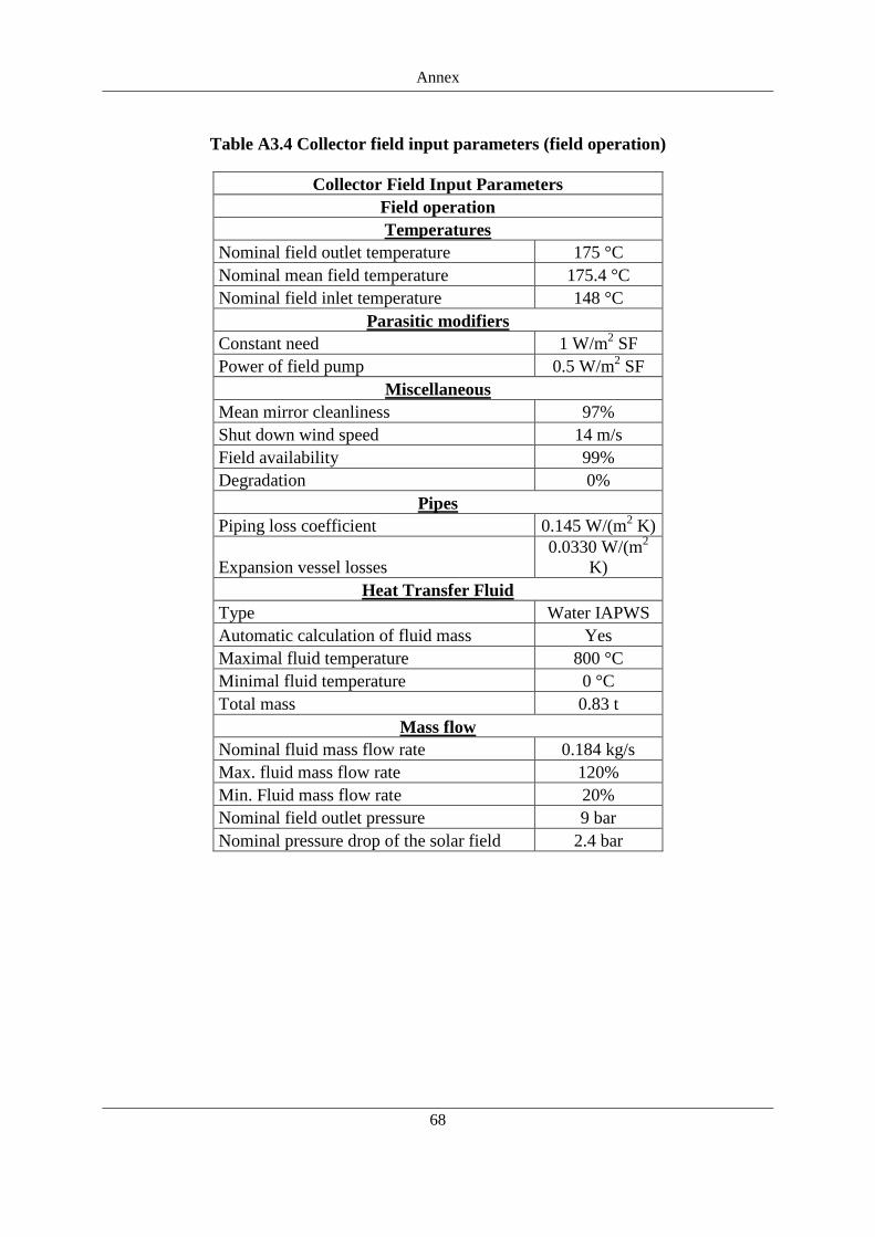
Annex

68

Table A3.4 Collector field input parameters (field operation)

Collector Field Input Parameters Field operation Temperatures

Nominal field outlet temperature 175 °C Nominal mean field temperature 175.4 °C Nominal field inlet temperature 148 °C

Parasitic modifiers Constant need 1 W/m2 SF Power of field pump 0.5 W/m2 SF

Miscellaneous Mean mirror cleanliness 97% Shut down wind speed 14 m/s Field availability 99% Degradation 0%

Pipes Piping loss coefficient 0.145 W/(m2 K)

Expansion vessel losses 0.0330 W/(m2

K) Heat Transfer Fluid

Type Water IAPWS Automatic calculation of fluid mass Yes Maximal fluid temperature 800 °C Minimal fluid temperature 0 °C Total mass 0.83 t

Mass flow Nominal fluid mass flow rate 0.184 kg/s Max. fluid mass flow rate 120% Min. Fluid mass flow rate 20% Nominal field outlet pressure 9 bar Nominal pressure drop of the solar field 2.4 bar

Annex

69

Table A3.5 Lookup table with input parameters for power block modelling in Greenius

Input parameters for power block modelling in Greenius name Zuccato ORC ZE60LT source DLR contact Greenius Team cooling_type 1 scaling 100 eff_mod_turbine 100 eff_mod_parasitics 100 aux_parasitics 0 cooling_parasitics 0 CO2_emmissions 0.23 SO2_emmisions 0 baseyear 2014 landuse 100 specific_investment_costs 5500 specific_OM_costs 0 specific_replacement_costs 0.02 specific_insurance_costs 0 guaranteetime 2 maximal_load 1 minimal_load 0.49 thermal_input_range 0 218 219 249 278 309 341 375 410 450 inlet_temperature_range 170 amb_temperature_range 20 amb_pressure_range 1 amb_humidity_range 30 condenser_pressure_range 0.08 load_range -1 design_conditions 450 170 20 1 30 0.1 -1

generator_output 0 0 25 29.9 35 41 46.3 52 58.8 66.3 parasitics_matrix 0 0 3.1 3.1 3.1 3.1 3.1 3.1 3.1 3.1 auxiliary_heat 0 0 0 0 0 0 0 0 0 0 HTF_inlet_temperature 160 160 160 160 160 160 160 160 160 160 HTF_outlet_temperature 0 0 80 80 80 80 80 80 80 80

70

References

71

References 1. Müller-Steinhagen, H. and F. Trieb, Concentrating solar power. A review of the technology.

Ingenia Inform QR Acad Eng, 2004. 18: p. 43-50. 2. International Energy Agency, Key world energy statistics2014: International Energy Agency. 3. Zervos, A., C. Lins, and J. Muth, RE-thinking 2050: a 100% renewable energy vision for the

European Union2010: EREC. 4. Pitz-Paal, R., et al., Solar Thermal Power Production. Transition to Renewable Energy

Systems, 2013: p. 307-338. 5. Barkai, M., et al., Universal Vacuum Collector (UVAC) Proceedings of the Solar 2002

American Solar Energy Society Conference. Reno, Nevada, 2002. 6. Winter, C.-J., R.L. Sizmann, and L.L. Vant-Hull, Solar power plants: fundamentals,

technology, systems, economics1991: Springer-Verlag New York. 7. Kalogirou, S.A., Solar thermal collectors and applications. Progress in energy and

combustion science, 2004. 30(3): p. 231-295. 8. Romero, M., R. Buck, and J.E. Pacheco, An update on solar central receiver systems, projects,

and technologies. Journal of solar energy engineering, 2002. 124(2): p. 98-108. 9. SolarPACES. CSP - How it Works. 2013 [cited 2014 September 24]; Available from:

http://www.solarpaces.org/csp-technology/csp-technology-general-information. 10. Timilsina, G.R., L. Kurdgelashvili, and P.A. Narbel, Solar energy: Markets, economics and

policies. Renewable and Sustainable Energy Reviews, 2012. 16(1): p. 449-465. 11. Valenzuela, L., et al., Control concepts for direct steam generation in parabolic troughs. Solar

energy, 2005. 78(2): p. 301-311. 12. Eck, M., et al., Applied research concerning the direct steam generation in parabolic troughs.

Solar energy, 2003. 74(4): p. 341-351. 13. Osuna, R., et al. PS10: A 11.0-MW solar tower power plant with saturated steam receiver. in

Proceedings of the 12th Solar PACES International Symposium on Concentrated Solar Power and Chemical Energy Technologies, Oaxaca, México, October. 2004.

14. Zarza, E., et al., INDITEP: The first pre-commercial DSG solar power plant. Solar energy, 2006. 80(10): p. 1270-1276.

15. Krüger, D., et al. Experiences with direct steam generation at the Kanchanaburi solar thermal power plant. in 18th SolarPACES Conference, Marrakech, Morocco. 2012.

16. Langenkamp, J., Revised LEC Projections and Discussion of Different DGS Benefits, 1998, Project DISS Technical Report DISS-SC–QA–02. Almerıa, Spain.

17. Pitz-Paal, R., et al., ECOSTAR roadmap document. DLR, Germany, 2005. 18. Zarza, E., et al., The DISS project: direct steam generation in parabolic trough systems.

Operation and maintenance experience and update on project status. Journal of solar energy engineering, 2002. 124(2): p. 126-133.

19. Zarza, E., DISS Phase II Final Report, 2002, EU Contract No. JOR3-CT98-0277. 20. Eck, M. and W.-D. Steinmann, Direct steam generation in parabolic troughs: first results of

the DISS project. Journal of solar energy engineering, 2002. 124(2): p. 134-139. 21. Eck, M. and E. Zarza. Assessment of operation modes for direct solar steam generation in

parabolic troughs. in 11th International Symposium on Solar Thermal Concentrating Technologies, Zurich. 2002.

22. SoltiguaTM. PTMx working principle. 2014 [cited 2014 August 1]; Available from: http://www.soltigua.com/prodotti/ptm/principio-funzionamento/.

23. Krüger, D., Kenissi, A., Schenk, H., Bouden, C., Baba, A., Oliveira, A., Soares, J., Rojas Bravo, E., Ben Cheikh, R. B., Orioli, F., Gasperini, D., Hennecke, K., Pre-Design of a Mini CSP plant. Energy Procedia, Submitted for publication (2014).

http://www.solarpaces.org/csp-technology/csp-technology-general-information

http://www.soltigua.com/prodotti/ptm/principio-funzionamento/

References

72

24. Coelho, B., et al., Biomass and central receiver system (CRS) hybridization: Volumetric air CRS and integration of a biomass waste direct burning boiler on steam cycle. Solar energy, 2012. 86(10): p. 2912-2922.

25. Birnbaum, J., et al., A direct steam generation solar power plant with integrated thermal storage. Journal of solar energy engineering, 2010. 132(3): p. 031014.

26. Montes, M., A. Abánades, and J. Martínez-Val, Performance of a direct steam generation solar thermal power plant for electricity production as a function of the solar multiple. Solar energy, 2009. 83(5): p. 679-689.

27. Ray, S. and G. Moss, Fluorochemicals as working fluids for small Rankine cycle power units. Advanced Energy Conversion, 1966. 6(2): p. 89-102.

28. Schuster, A., et al., Energetic and economic investigation of Organic Rankine Cycle applications. Applied Thermal Engineering, 2009. 29(8): p. 1809-1817.

29. Borsukiewicz-Gozdur, A. and W. Nowak, Comparative analysis of natural and synthetic refrigerants in application to low temperature Clausius–Rankine cycle. Energy, 2007. 32(4): p. 344-352.

30. Drescher, U. and D. Brüggemann, Fluid selection for the Organic Rankine Cycle (ORC) in biomass power and heat plants. Applied Thermal Engineering, 2007. 27(1): p. 223-228.

31. VDI-Gesellschaft Verfahrenstechnik und Chemieingenieurwesen, V., VDI Heat Atlas. VDI-Buch, Springer, 2010.

32. Sarco, S., The steam and condensate loop book, 2007, Spirax-Sarco. 33. Grote, K.-H., DUBBEL Taschenbuch für den Maschinenbau2011: Springer DE. 34. Eck, M. and W.-D. Steinmann. Modeling and design of direct solar steam generating

collector fields. in ASME 2004 International Solar Energy Conference. 2004. American Society of Mechanical Engineers.

35. Herrmann, U., Untersuchung zur Rohrwandbenetzung bei der Dampferzeugung in horizontalen und geneigten Parabolrinnen-Solarkollektoren2004: Flagsol.

36. Odeh, S., G. Morrison, and M. Behnia, Modelling of parabolic trough direct steam generation solar collectors. Solar energy, 1998. 62(6): p. 395-406.

37. Bohl, W., Technische Strömungslehre, 10. Auflage, Würzburg, 1994, Vogel Verlag und Druck KG.

38. Herning, F., Stoffströme in Rohrleitungen1966: VDI-Verlag. 39. Qu, M., D.H. Archer, and H. Yin. A linear parabolic trough solar collector performance

model. in ASME 2007 Energy Sustainability Conference. 2007. American Society of Mechanical Engineers.

40. Keenan, J., et al., Steam tables (International edition-metric units), 1969, Wiley, New York. 41. Pipe Flow Calculations. Water properties table - density, specific heat, viscosity. 2014 [cited

2014 August 4]; Available from: http://www.pipeflowcalculations.com/tables/water.php. 42. Duffie, J.A. and W.A. Beckman, Solar engineering of thermal processes. NASA STI/Recon

Technical Report A, 1980. 81: p. 16591. [39] [42]

http://www.pipeflowcalculations.com/tables/water.php

Fachhochschule Aachen - elib.dlr.de Leonel Reyes Ochoa.pdf · To the FH Aachen for having enriched my academic formation and professional expectations. To CONACYT and DAAD which made

Documents