Face Recognition with Local Binary Patterns, Spatial Pyramid Histograms and Naive Bayes Nearest Neighbor Classification

Face Recognition with Local Binary Patterns, Spatial Pyramid Histograms andNaive Bayes Nearest Neighbor classification

Daniel Maturana, Domingo Mery and Alvaro SotoDepartamento de Ciencias de la Computacion

Pontificia Universidad CatolicaSantiago, Chile

Email: {dimatura, dmery, asoto}@uc.cl

Abstract—Face recognition algorithms commonly assumethat face images are well aligned and have a similar pose– yet in many practical applications it is impossible to meetthese conditions. Therefore extending face recognition to un-constrained face images has become an active area of research.

To this end, histograms of Local Binary Patterns (LBP)have proven to be highly discriminative descriptors for facerecognition. Nonetheless, most LBP-based algorithms use arigid descriptor matching strategy that is not robust againstpose variation and misalignment.

We propose two algorithms for face recognition that are de-signed to deal with pose variations and misalignment. We alsoincorporate an illumination normalization step that increasesrobustness against lighting variations. The proposed algorithmsuse descriptors based on histograms of LBP and performdescriptor matching with spatial pyramid matching (SPM) andNaive Bayes Nearest Neighbor (NBNN), respectively. Our con-tribution is the inclusion of flexible spatial matching schemesthat use an image-to-class relation to provide an improvedrobustness with respect to intra-class variations.

We compare the accuracy of the proposed algorithms againstAhonen’s original LBP-based face recognition system and twobaseline holistic classifiers on four standard datasets. Ourresults indicate that the algorithm based on NBNN outperformsthe other solutions, and does so more markedly in presence ofpose variations.

Keywords-face recognition; local binary patterns; naiveBayes; nearest neighbor; spatial pyramid.

I. INTRODUCTION

Most face recognition algorithms are designed to workbest with well aligned, well illuminated, and frontal poseface images. In many possible applications, however, it isnot possible to meet these conditions. Some examples aresurveillance, automatic tagging, and human robot interac-tion. Therefore, there have been many recent efforts todevelop algorithms that perform well with unconstrainedface images [1]–[4].

In this context, the of use local appearance descriptorssuch as Gabor jets [5], [6], SURF [7], SIFT [8], [9], HOG[10] and histograms of Local Binary Patterns [11] havebecome increasingly common. Algorithms that use localappearance descriptors are more robust against occlusion,expression variation, pose variation and small sample sizesthan traditional holistic algorithms [4], [5].

In this work we will focus on descriptors based on LocalBinary Patterns (LBP), as they are simple, computationallyefficient and have proved to be highly effective featuresfor face recognition [3], [4], [12], [13]. Nonetheless, themethods described in this paper can be readily adapted tooperate with alternative local descriptors.

Within LBP-based algorithms, most of the face recogni-tion algorithms using LBP follow the approach proposedby Ahonen et al in [12]. In this approach the face imageis divided into a grid of small of non overlapping regions,where a histogram of the LBP for each region is constructed.The similarity of two images is then computed by summingthe similarity of histograms from corresponding regions.

One drawback of the previous method is that it assumesthat a given image region corresponds to the same part of theface in all the faces in the dataset. This is only possible if theface images are fully frontal, scaled, and aligned properly. Inaddition, while LBP are invariant against monotonic gray-scale transformations, they are still affected by illuminationchanges that induce non monotonic gray-scale changes suchas self shadowing [17].

In this paper, we propose and compare two algorithmsfor face recognition that are specially designed to dealwith moderate pose variations and misaligned faces. Thesealgorithms are based on previous techniques from the objectrecognition literature: spatial pyramid matching [14], [15]and Naive Bayes Nearest Neighbors (NBNN) [16]. Ourmain contribution is the inclusion of flexible spatial match-ing schemes based on an “image-to-class” relation whichprovides an improved robustness with respect to intra-classvariations. These matching schemes use spatially dependentvariations of the “bag of words” models with LBP histogramdescriptors. As a further refinement, we also incorporatea state of the art illumination compensation algorithm toimprove robustness against illumination changes [17].

This paper is organized as follows. Section II discussesthe details of our approach. Section III-C shows the resultsof applying our methodology to standard datasets. Finally,section IV presents the main conclusions of this work.

II. ALGORITHMS

We start by summarizing the main common steps of thealgorithms used in this work. Then we describe each stepin detail. The proposed face recognition process consists offour main parts:

1) Preprocessing: We begin by applying the Tan andTriggs’ illumination normalization algorithm [17] tocompensate for illumination variation in the face im-age. No further preprocessing, such as face alignment,is performed.

2) LBP operator application: In the second stage LBP arecomputed for each pixel, creating a fine scale texturaldescription of the image.

3) Local feature extraction: Local features are createdby computing histograms of LBP over local imageregions.

4) Classification: Each face image in test set is classifiedby comparing it against the face images in the trainingset. The comparison is performed using the localfeatures obtained in the previous step.

The first two steps are shared by all the algorithms. Thealgorithms we explore in this work vary in how they performthe last two steps, as we detail in section II-C.

A. Preprocessing

Illumination accounts for a large part of the variationin appearance of face images [18]. Various preprocessingmethods have been created to compensate for this variation[19]. We have chosen to use the method proposed by Tanand Triggs [17] since it is simple, efficient, and has beenshown to work well with local binary patterns.

The algorithm consists of four steps:

1) Gamma correction to enhance the dynamic range ofdark regions and compress light areas and highlights.We use γ = 0.2.

2) Difference of Gaussians (DoG) filtering that acts asa “band pass”, partially suppressing high frequencynoise and low frequency illumination variation. Forthe width of the Gaussian kernels we use σ0 = 1.0and σ1 = 2.0.

3) Contrast equalization to rescale image intensities inorder to standardize intensity variations. The equal-ization is performed in two steps:

I(x, y)← I(x′, y′)(mean(| I(x′, y′)|a))1/a

I(x, y)← I(x′, y′)(mean(min(τ, | I(x′, y′)|)a))1/a

where I(x, y) refers to the pixel in position (x, y) ofthe image I and τ and a are parameters. We use a =0.1 and τ = 10.

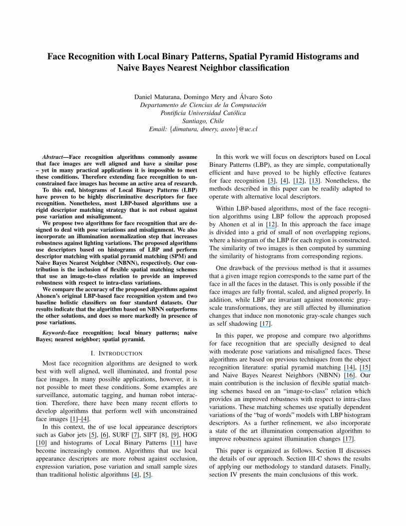
Figure 1. The upper row shows three images of a subject from the Yale Bdataset under different lighting conditions. The bottom row shows the sameimages after processing with Tan and Triggs’ illumination normalizationalgorithm. Appearance variation due to lighting is drastically reduced.

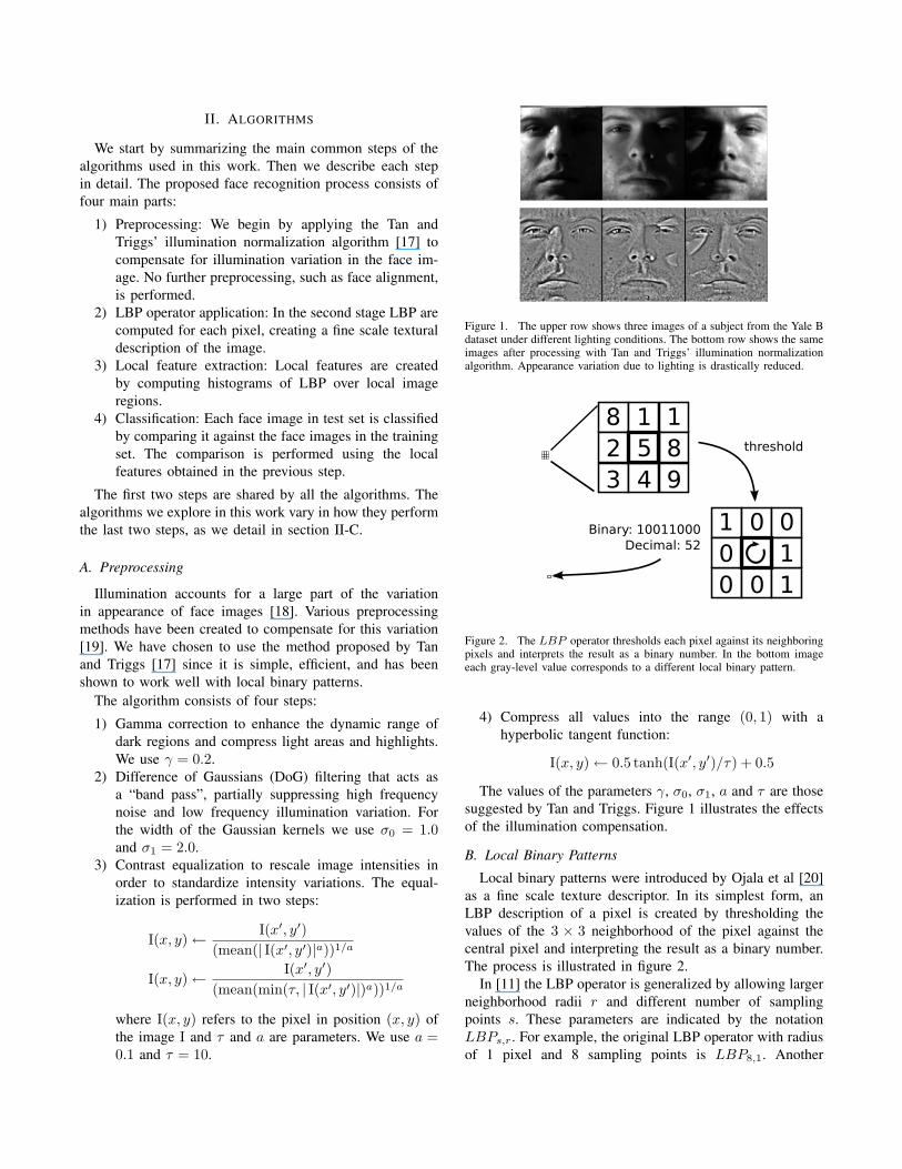
Figure 2. The LBP operator thresholds each pixel against its neighboringpixels and interprets the result as a binary number. In the bottom imageeach gray-level value corresponds to a different local binary pattern.

4) Compress all values into the range (0, 1) with ahyperbolic tangent function:

I(x, y)← 0.5 tanh(I(x′, y′)/τ) + 0.5

The values of the parameters γ, σ0, σ1, a and τ are thosesuggested by Tan and Triggs. Figure 1 illustrates the effectsof the illumination compensation.

B. Local Binary Patterns

Local binary patterns were introduced by Ojala et al [20]as a fine scale texture descriptor. In its simplest form, anLBP description of a pixel is created by thresholding thevalues of the 3 × 3 neighborhood of the pixel against thecentral pixel and interpreting the result as a binary number.The process is illustrated in figure 2.

In [11] the LBP operator is generalized by allowing largerneighborhood radii r and different number of samplingpoints s. These parameters are indicated by the notationLBPs,r. For example, the original LBP operator with radiusof 1 pixel and 8 sampling points is LBP8,1. Another

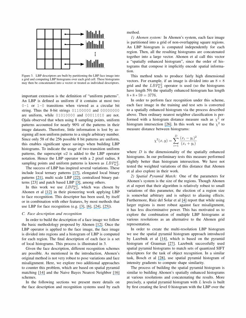
Figure 3. LBP descriptors are built by partitioning the LBP face image intoa grid and computing LBP histograms over each grid cell. These histogramsmay then be concatenated into a vector or treated as individual descriptors.

important extension is the definition of “uniform patterns”.An LBP is defined as uniform if it contains at most two0-1 or 1-0 transitions when viewed as a circular bitstring. Thus the 8-bit strings 01100000 and 00000000are uniform, while 01010000 and 00011010 are not.Ojala observed that when using 8 sampling points, uniformpatterns accounted for nearly 90% of the patterns in theirimage datasets. Therefore, little information is lost by as-signing all non uniform patterns to a single arbitrary number.Since only 58 of the 256 possible 8 bit patterns are uniform,this enables significant space savings when building LBPhistograms. To indicate the usage of two-transition uniformpatterns, the superscript u2 is added to the LBP operatornotation. Hence the LBP operator with a 2 pixel radius, 8sampling points and uniform patterns is known as LBPu2

8,2.The success of LBP has inspired several variations. These

include local ternary patterns [17], elongated local binarypatterns [21], multi scale LBP [22], centralized binary pat-terns [23] and patch based LBP [3], among others.

In this work we use LBPu28,2, which was chosen by

Ahonen et al [12] in their pioneering work applying LBPto face recognition. This descriptor has been used, by itselfor in combination with other features, by most methods thatuse LBP for face recognition (e.g. [3], [6], [24], [25]).

C. Face description and recognition

In order to build the description of a face image we followthe basic methodology proposed by Ahonen [12]. Once theLBP operator is applied to the face image, the face imageis divided into regions and a histogram of LBP is computedfor each region. The final description of each face is a setof local histograms. This process is illustrated in 3.

Given the face description, different recognition schemesare possible. As mentioned in the introduction, Ahonen’soriginal method is not very robust to pose variations and facemisalignment. Here, we explore two additional approachesto counter this problem, which are based on spatial pyramidmatching [14] and the Naive Bayes Nearest Neighbor [16]schemes.

In the following sections we present more details onthe face description and recognition systems used by each

method.1) Ahonen system: In Ahonen’s system, each face image

is partitioned into a grid of non-overlapping square regions.An LBP histogram is computed independently for eachregion. Then, all the resulting histograms are concatenatedtogether into a large vector. Ahonen et al call this vectora “spatially enhanced histogram”, since the order of his-tograms that compose it implicitly encode spatial informa-tion.

This method tends to produce fairly high dimensionalvectors. For example, if an image is divided into an 8 × 8grid and the LBPu2

8,2 operator is used (so the histogramshave length 59) the spatially enhanced histogram has length8 ∗ 8 ∗ 59 = 3776.

In order to perform face recognition under this scheme,each face image in the training and test sets is convertedto a spatially enhanced histogram via the process describedabove. Then ordinary nearest neighbor classification is per-formed with a histogram distance measure such as χ2 orhistogram intersection [26]. In this work we use the χ2 tomeasure distance between histograms:

χ2(x, y) =D∑i=1

(xi − yi)2

(xi + yi)

where D is the dimensionality of the spatially enhancedhistograms. In our preliminary tests this measure performedslightly better than histogram intersection. We have nottested the weighted variations of this distance that Ahonenet al also explore in their work.

2) Spatial Pyramid Match: One of the parameters forAhonen’s system is the size of the regions. Though Ahonenet al report that their algorithm is relatively robust to smallvariations of this parameter, the election of a region sizeis somewhat arbitrary and is subject to aliasing effects.Furthermore, Ruiz del Solar et al [4] report that while usinglarger regions is more robust against face misalignment,it has less discriminative power. This has motivated us toexplore the combination of multiple LBP histograms atvarious resolutions as an alternative to the Ahonen gridrepresentation.

In order to create the multi-resolution LBP histogramwe use the spatial pyramid histogram approach introducedby Lazebnik et al [14], which is based on the pyramidhistogram of Grauman [27]. Lazebnik successfully usedspatial pyramid histograms to match sets of quantized SIFTdescriptors for the task of object recognition. In a similartask, Bosch et al [28], use spatial pyramid histogram ofintensity gradients to compute shape similarity.

The process of building the spatial pyramid histogram issimilar to building Ahonen’s spatially enhanced histogramsat various resolutions and concatenating the results. Moreprecisely, a spatial pyramid histogram with L levels is builtby first creating the level 0 histogram with the LBP over the

entire image. Next, the image is divided in four equal sizedregions and a level 1 LBP histogram is computed for eachregion. The process is repeated by recursively subdividingeach region and computing level l histograms in each regionuntil the desired level L is reached. A simple calculationshows that there will 22l level l histograms and that bysumming this number over l = 0, . . . , L a spatial pyramidhistogram with L levels will have a total of (22L+2 − 1)/3histograms. As in Ahonen’s method all these histograms areconcatenated together into a large vector 1. For example,if we describe a face image with a three level spatialpyramid (L = 3) and LBPu2

8,1, the resulting vector has length((22∗3+2 − 1)/3) ∗ 59 = 5015.

For classification a nearest neighbor classifier is used, asin the Ahonen system. However, to compare histograms weuse a distance based on the Pyramid Match Kernel [27] withsome of the modifications used by Bosch [28] instead ofplain χ2. The motivation behind this distance is that matchesamong histograms at coarser resolutions should be givenless weight, because it is less likely than they come fromcorresponding face parts. Specifically, if we have two spatialpyramids x and y, and we denote by δl the sum of thedistance between all the histograms at level l (we use χ2,as in [28]) then the distance is calculated as

d(x, y) =δ02L

+L∑l=1

δl2L−l+1

3) Naive Bayes Nearest Neighbor: While we expectspatial pyramid histograms to be more robust to facemisalignment and pose variation than Ahonen’s spatiallyenhanced histograms, they still have a rigid approach tospatial matching. As in Ahonen’s method, when two faceimages are compared each local feature in one image iscompared against the local feature found at the same positionin the other image. This suggests a more flexible spatialmatching approach, wherein local features from one imageare allowed to be matched to local features found in differentpositions from other images.

This idea evokes the “bag of visual words” approachthat has proved successful in object recognition and sceneclassification (e.g. [15], [29]). However, it seems unwise todiscard all spatial information given that it clearly is usefulfor visual recognition, as shown by work incorporatingspatial information into the bag of words model [14], [30].Another disadvantage of the bag of words model is thatit requires a codebook creation stage which tends to losediscriminative information, as shown in [16].

In this paper we test an intermediate approach, introducedby Boiman et al [16] in the context of visual object recog-

1We modify slightly the construction process of the pyramid used byLazebnik in order to emphasize the similarities with Ahonen’s grid spatiallyenhanced histogram, but by modifying the kernel function appropriately theresults are equivalent. In particular, instead of treating the LBP “channels”separately we interleave them.

nition using local descriptors. Since the method is based onthe Nearest Neighbor classifier and makes a naive Bayesassumption, it is named “Naive Bayes Nearest Neighbor”(NBNN).

NBNN assumes images are represented by sets of localfeatures. Boiman’s work uses a combination of variousvisual descriptors, including SIFT [8] and Shape Contexts[32]. In this paper we use the aforementioned LBP his-tograms over local regions as descriptors. To make thealgorithms comparable we use the same grid-based regionsas the Ahonen method. Nonetheless, instead of concate-nating the histograms of each region into a single vector,each histogram is kept separate. To keep track of spatialinformation the histograms are augmented with the (x, y)coordinates of the center of its region. Therefore under thisscheme each face is not described by a single vector, as inthe previous two approaches, but by a set of vectors.

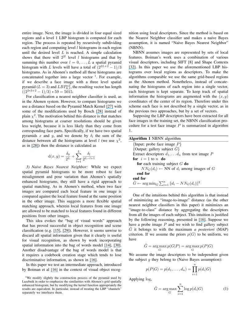
Supposing the LBP descriptors have been extracted for allface images in the training set, the NBNN classification pro-cedure for a test face image P is summarized in algorithm1.

Algorithm 1 NBNN algorithm{Input: probe face image P}{Output: gallery subject G}Extract descriptors d1, . . . dn from test image Pfor i = 1 to n do

for each training subject G doNNG(di) ← NN of di among images of G

end forend forG← arg minG

∑ni=1 ‖di −NNG(di)‖2

One of the intuitions behind this algorithm is that insteadof minimizing an “image-to-image” distance (as the othernearest neighbor classifiers in this paper) it minimizes an“image-to-class” distance by aggregating the descriptorsfrom all the images of each subject. This intuition is justifiedby the following reasoning, presented in [16]. Suppose wehave a probe image P and we wish to find gallery subjectG it belongs to with the maximum a posteriori (MAP)criterion. If we assume the priors p(G) to be uniform, wehave

G = arg maxG

p(G|P ) = arg maxG

p(P |G)

We assume the image descriptors to be independent giventhe subject g they belong to (Naive Bayes assumption):

p(P |G) = p(d1, . . . , dn) =n∏i=1

p(di|G)

Applying log,

G = arg maxG

n∑i=1

log p(di|G) (1)

Rewriting the right hand side using the law of total proba-bility,

G = arg maxG

∑d

p(d|P ) log p(d|G)

where we sum over the space of all possible descriptors d.By subtracting the constant term

∑d p(d|P ) log p(d|P ) on

the right side (which does not affect G) and rearranging,

G = arg maxG

(∑d

p(d|P ) logp(d|G)p(d|P )

)= arg min

GKL (p(d|P )‖p(d|G))

where KL(·‖·) is the Kullback-Leibler divergence betweentwo distributions. Thus in this case the MAP criterion isequivalent to minimizing the KL divergence between thedescriptor distributions of P and the descriptor distributionof the subject G (i.e. the “image-to-class” distance).

We have not specified how to calculate (1), and inparticular p(d|G). The NBNN approach is to approximatethe Parzen likelihood estimator for p(d|G) with the r nearestneighbors NNj , j = 1 . . . r of d belonging to G:

pNN (d|G) =1L

r∑j

K(d− dGNNj) (2)

where K is the Gaussian Parzen kernel function: K(d −dGj = exp( 1

2σ2 ‖d − dGj ‖2). If r = 1, corresponding to asingle nearest neighbor approximation, (2) becomes a simpleexpression and the constant factors such as σ2 may beignored. Then (1) becomes:

G = arg minG

n∑i=1

‖di −NNG(di)‖2

which is the expression used in algorithm 1.Boiman et al incorporate spatial information into this

scheme by appending (x, y) pixel coordinates to each de-scriptor, scaled by a factor α. Thus the squared euclideandistance between two descriptors d1 and d2 at positions(x1, y1) and (x2, y2) becomes∑

i

(d1i − d2i)2 + α((x1 − x2)2 + (y1 − y2)2

)The value of α determines the weight given to spatialinformation when matching descriptors. If the value is set to0 spatial information is completely disregarded. This may bebeneficial when dealing with very large pose variations butprobably increases the chances of mismatches. In the otherextreme, setting α to a very large value forces descriptorsto be matched exclusively with descriptors from the samespatial location, as in Ahonen’s method.

We set this parameter by cross-validating in a small in-house face dataset. We found α = 1 to be a good choiceand used this value with all the datasets. Since not alldatasets use the same image size, to make the influence of

α commensurate across datasets we linearly scale all (x, y)coordinates so the upper left corner of the image is at (0, 0)and the lower right corner is at (1, 1).

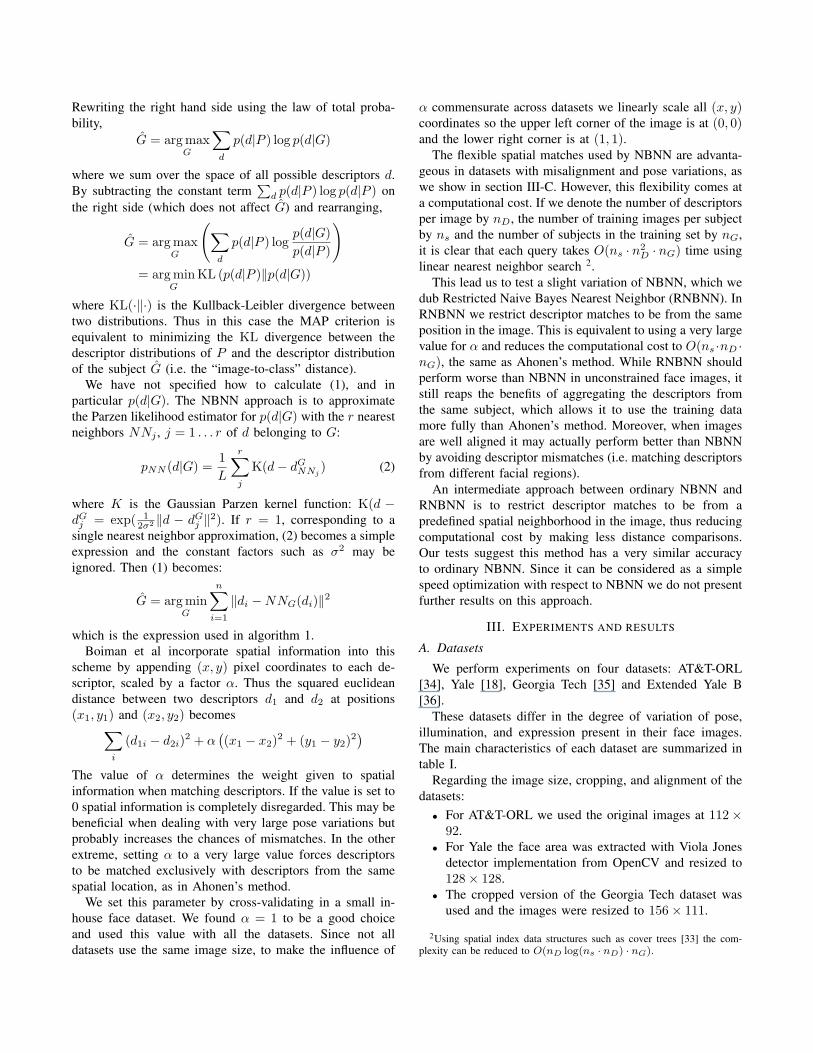
The flexible spatial matches used by NBNN are advanta-geous in datasets with misalignment and pose variations, aswe show in section III-C. However, this flexibility comes ata computational cost. If we denote the number of descriptorsper image by nD, the number of training images per subjectby ns and the number of subjects in the training set by nG,it is clear that each query takes O(ns · n2

D · nG) time usinglinear nearest neighbor search 2.

This lead us to test a slight variation of NBNN, which wedub Restricted Naive Bayes Nearest Neighbor (RNBNN). InRNBNN we restrict descriptor matches to be from the sameposition in the image. This is equivalent to using a very largevalue for α and reduces the computational cost to O(ns ·nD ·nG), the same as Ahonen’s method. While RNBNN shouldperform worse than NBNN in unconstrained face images, itstill reaps the benefits of aggregating the descriptors fromthe same subject, which allows it to use the training datamore fully than Ahonen’s method. Moreover, when imagesare well aligned it may actually perform better than NBNNby avoiding descriptor mismatches (i.e. matching descriptorsfrom different facial regions).

An intermediate approach between ordinary NBNN andRNBNN is to restrict descriptor matches to be from apredefined spatial neighborhood in the image, thus reducingcomputational cost by making less distance comparisons.Our tests suggest this method has a very similar accuracyto ordinary NBNN. Since it can be considered as a simplespeed optimization with respect to NBNN we do not presentfurther results on this approach.

III. EXPERIMENTS AND RESULTS

A. Datasets

We perform experiments on four datasets: AT&T-ORL[34], Yale [18], Georgia Tech [35] and Extended Yale B[36].

These datasets differ in the degree of variation of pose,illumination, and expression present in their face images.The main characteristics of each dataset are summarized intable I.

Regarding the image size, cropping, and alignment of thedatasets:• For AT&T-ORL we used the original images at 112×

92.• For Yale the face area was extracted with Viola Jones

detector implementation from OpenCV and resized to128× 128.

• The cropped version of the Georgia Tech dataset wasused and the images were resized to 156× 111.

2Using spatial index data structures such as cover trees [33] the com-plexity can be reduced to O(nD log(ns · nD) · nG).

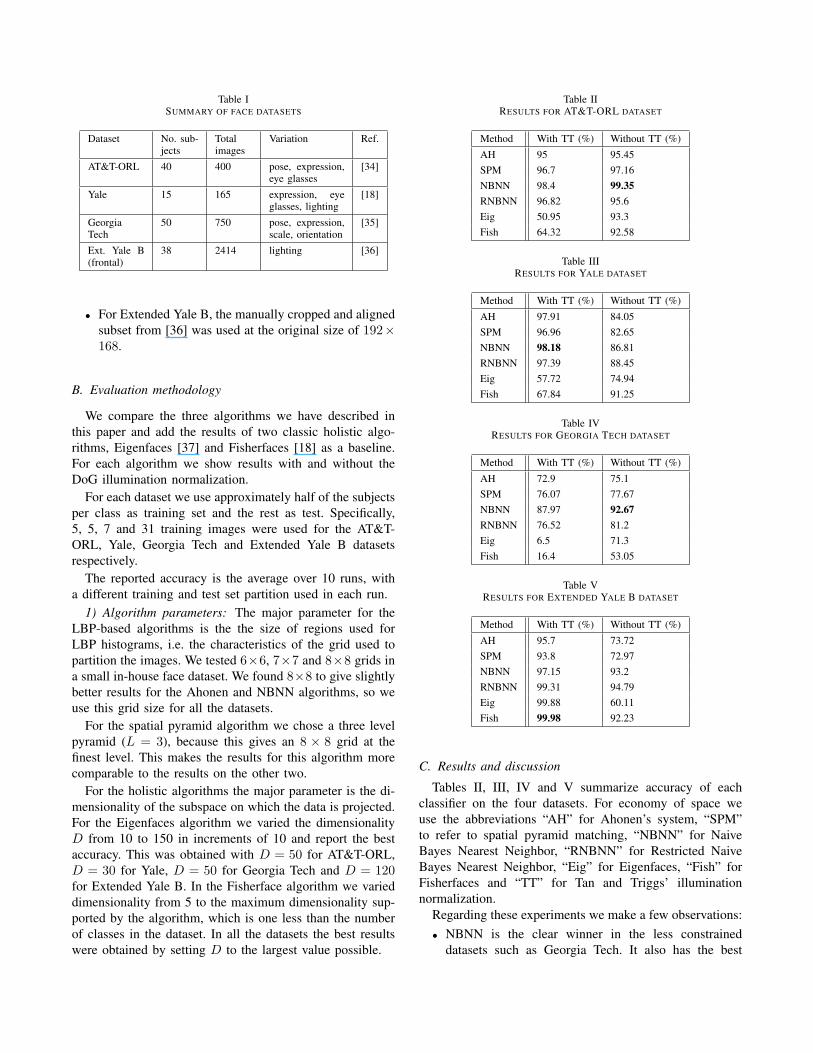
Table ISUMMARY OF FACE DATASETS

Dataset No. sub-jects

Totalimages

Variation Ref.

AT&T-ORL 40 400 pose, expression,eye glasses

[34]

Yale 15 165 expression, eyeglasses, lighting

[18]

GeorgiaTech

50 750 pose, expression,scale, orientation

[35]

Ext. Yale B(frontal)

38 2414 lighting [36]

• For Extended Yale B, the manually cropped and alignedsubset from [36] was used at the original size of 192×168.

B. Evaluation methodology

We compare the three algorithms we have described inthis paper and add the results of two classic holistic algo-rithms, Eigenfaces [37] and Fisherfaces [18] as a baseline.For each algorithm we show results with and without theDoG illumination normalization.

For each dataset we use approximately half of the subjectsper class as training set and the rest as test. Specifically,5, 5, 7 and 31 training images were used for the AT&T-ORL, Yale, Georgia Tech and Extended Yale B datasetsrespectively.

The reported accuracy is the average over 10 runs, witha different training and test set partition used in each run.

1) Algorithm parameters: The major parameter for theLBP-based algorithms is the the size of regions used forLBP histograms, i.e. the characteristics of the grid used topartition the images. We tested 6×6, 7×7 and 8×8 grids ina small in-house face dataset. We found 8×8 to give slightlybetter results for the Ahonen and NBNN algorithms, so weuse this grid size for all the datasets.

For the spatial pyramid algorithm we chose a three levelpyramid (L = 3), because this gives an 8 × 8 grid at thefinest level. This makes the results for this algorithm morecomparable to the results on the other two.

For the holistic algorithms the major parameter is the di-mensionality of the subspace on which the data is projected.For the Eigenfaces algorithm we varied the dimensionalityD from 10 to 150 in increments of 10 and report the bestaccuracy. This was obtained with D = 50 for AT&T-ORL,D = 30 for Yale, D = 50 for Georgia Tech and D = 120for Extended Yale B. In the Fisherface algorithm we varieddimensionality from 5 to the maximum dimensionality sup-ported by the algorithm, which is one less than the numberof classes in the dataset. In all the datasets the best resultswere obtained by setting D to the largest value possible.

Table IIRESULTS FOR AT&T-ORL DATASET

Method With TT (%) Without TT (%)

AH 95 95.45SPM 96.7 97.16NBNN 98.4 99.35RNBNN 96.82 95.6Eig 50.95 93.3Fish 64.32 92.58

Table IIIRESULTS FOR YALE DATASET

Method With TT (%) Without TT (%)

AH 97.91 84.05SPM 96.96 82.65NBNN 98.18 86.81RNBNN 97.39 88.45Eig 57.72 74.94Fish 67.84 91.25

Table IVRESULTS FOR GEORGIA TECH DATASET

Method With TT (%) Without TT (%)

AH 72.9 75.1SPM 76.07 77.67NBNN 87.97 92.67RNBNN 76.52 81.2Eig 6.5 71.3Fish 16.4 53.05

Table VRESULTS FOR EXTENDED YALE B DATASET

Method With TT (%) Without TT (%)

AH 95.7 73.72SPM 93.8 72.97NBNN 97.15 93.2RNBNN 99.31 94.79Eig 99.88 60.11Fish 99.98 92.23

C. Results and discussion

Tables II, III, IV and V summarize accuracy of eachclassifier on the four datasets. For economy of space weuse the abbreviations “AH” for Ahonen’s system, “SPM”to refer to spatial pyramid matching, “NBNN” for NaiveBayes Nearest Neighbor, “RNBNN” for Restricted NaiveBayes Nearest Neighbor, “Eig” for Eigenfaces, “Fish” forFisherfaces and “TT” for Tan and Triggs’ illuminationnormalization.

Regarding these experiments we make a few observations:• NBNN is the clear winner in the less constrained

datasets such as Georgia Tech. It also has the best

performance in Yale and AT&T-ORL. However, inExtended Yale B with illumination normalization itfalls behind the holistic algorithms (though it performsbetter than them with no illumination normalization).This is explained by the fact that Extended Yale Bsubset is a very well aligned dataset which only variesillumination, a situation where holistic algorithms, andFisherfaces in particular, work well.

• RNBNN performed somewhat better than the Ahonenalgorithm, specially when illumination normalizationis not used. As expected, the performance of RBNNsuffers in less constrained datasets. On the other hand,in the well aligned Yale B dataset it actually workedbetter than ordinary NBNN and was the best algorithmwith no illumination normalization.

• Spatial pyramid histograms perform slightly better thanAhonen’s method in the less constrained datasets. How-ever, it performed slightly worse in the well alignedExtended Yale B dataset as well as the Yale dataset.This suggests that most of the discriminative power ofthe pyramids is in the highest level.

• In face datasets with large illumination variations (Yaleand Extended Yale B) Tan and Triggs’ illuminationnormalization algorithm boosts the accuracy of LBP-based classifiers significantly. Holistic classifiers onlybenefited in Extended Yale B. In the rest the illumina-tion normalization lowers their accuracy to a surprisingdegree. We found that in these cases the decrease wasinversely proportional to the width of the DoG bandpassfilter.In face datasets with little or no lighting variation, LBP-based perform slightly worse with Tan and Triggs’algorithm, while the holistic algorithms still performsignificantly worse.

• The behavior of RNBNN and NBNN in the ExtendedYale B dataset with no illumination normalization isinteresting; they outperform the other LBP-based al-gorithms by a 20% margin. This is a consequence ofaggregating the descriptors for each class, because itallows each face region to be matched to a similarlyilluminated face region from the training set, in a cer-tain sense inferring a new face by “composing pieces”from various face images.

IV. CONCLUSIONS AND FUTURE WORK

Our main result is that the NBNN algorithm improvesperformance substantially with respect to the original LBP-based algorithm when used in relatively unconstrained facedatasets. NBNN also outperforms the original LBP algo-rithm even when faces are frontal and well aligned, thoughby a smaller margin. This improvements may be attributedto the flexible spatial matching scheme and the use of the“image-to-class” distance, which makes a better use of thetraining data than the “image-to-image” distance.

A. Future work

One of the drawbacks of NBNN is the increase in com-putational cost relative to the original LBP based algorithm.Since this cost is caused by the large amount of nearestneighbor queries it would be beneficial to speed up nearestneighbor queries with spatial index data structures such ascover trees [33] or locality sensitive hashing [38].

Another interesting avenue of research is to complementor replace the LBPu2

8,2 histogram descriptors with other localdescriptors, such as SIFT [8], SURF [7] or one of the manyLBP variations. Furthermore, we are currently exploringstrategies to learn a discriminative LBP-like descriptor fromthe data itself.

It would also be of interest to find a better alternativeto the grid-based regions used in this paper. The gridpartition has no natural relation to the shape of the face andsuffers from quantization effects. One possibility is to detect“interesting” facial regions (such as the eyebrows, nose andmouth) and extract descriptors in these selected regions.

ACKNOWLEDGMENT

This work was partially funded by FONDECYTgrant 1095140 and LACCIR Virtual Institute grant No.R1208LAC005 (http://www.laccir.org).

REFERENCES

[1] J. Wright and G. Hua, “Implicit elastic matching with randomprojections for Pose-Variant face recognition,” in Proc. CVPR,2009.

[2] P. Dreuw, P. Steingrube, H. Hanselmann, and H. Ney, “SURF-Face: face recognition under viewpoint consistency con-straints,” in British Machine Vision Conference, London, UK,Sep. 2009.

[3] L. Wolf, T. Hassner, and Y. Taigman, “Descriptor basedmethods in the wild,” in Proc. ECCV, 2008.

[4] J. Ruiz-del-Solar, R. Verschae, and M. Correa, “Recogni-tion of faces in unconstrained environments: A comparativestudy,” EURASIP Journal on Advances in Signal Processing,vol. 2009, pp. 1–20, 2009.

[5] J. Zou, Q. Ji, and G. Nagy, “A comparative study of localmatching approach for face recognition,” Image Processing,IEEE Transactions on, vol. 16, no. 10, pp. 2617–2628, 2007.

[6] X. Tan and B. Triggs, “Fusing gabor and LBP feature sets forKernel-Based face recognition,” in Analysis and Modeling ofFaces and Gestures, 2007, pp. 235–249.

[7] H. Bay, T. Tuytelaars, and L. V. Gool, “Surf: Speeded uprobust features,” Lecture notes in computer science, vol. 3951,p. 404, 2006.

[8] D. G. Lowe, “Distinctive image features from Scale-Invariantkeypoints,” Int. J. Comput. Vision, vol. 60, no. 2, pp. 91–110,2004.

[9] M. Bicego, A. Lagorio, E. Grosso, and M. Tistarelli, “On theuse of SIFT features for face authentication,” in Proceedingsof the 2006 Conference on Computer Vision and PatternRecognition Workshop. IEEE Computer Society, 2006, p. 35.

[10] A. Albiol, D. Monzo, A. Martin, J. Sastre, and A. Albiol,“Face recognition using HOG-EBGM,” Pattern Recogn. Lett.,vol. 29, no. 10, pp. 1537–1543, 2008.

[11] T. Ojala, M. Pietikainen, and T. Maenpaa, “Gray scale androtation invariant texture classification with local binary pat-terns,” Lecture Notes in Computer Science, vol. 1842, p.404420, 2000.

[12] T. Ahonen, A. Hadid, and M. Pietikainen, “Face descriptionwith local binary patterns: Application to face recognition,”IEEE Transactions on Pattern Analysis and Machine Intelli-gence, vol. 28, no. 12, pp. 2037–2041, 2006.

[13] Y. Rodriguez and S. Marcel, “Face authentication usingadapted local binary pattern histograms,” Lecture Notes inComputer Science, vol. 3954, p. 321, 2006.

[14] S. Lazebnik, C. Schmid, and J. Ponce, “Beyond bags offeatures: Spatial pyramid matching for recognizing naturalscene categories,” in Proceedings of the 2006 IEEE Com-puter Society Conference on Computer Vision and PatternRecognition - Volume 2. IEEE Computer Society, 2006, pp.2169–2178.

[15] A. Bosch, A. Zisserman, and X. Muoz, “Scene classificationvia pLSA,” in Computer Vision ECCV 2006, 2006, pp. 517–530.

[16] O. Boiman, E. Shechtman, and M. Irani, “In defense ofNearest-Neighbor based image classification,” in ComputerVision and Pattern Recognition, 2008. CVPR 2008. IEEEConference on, 2008, pp. 1–8.

[17] X. Tan and B. Triggs, “Enhanced local texture feature sets forface recognition under difficult lighting conditions,” LectureNotes in Computer Science, vol. 4778, p. 168, 2007.

[18] P. N. Belhumeur, J. P. Hespanha, and D. J. Kriegman,“Eigenfaces vs. fisherfaces: recognition using class specificlinearprojection,” IEEE Transactions on pattern analysis andmachine intelligence, vol. 19, no. 7, pp. 711–720, 1997.

[19] J. Ruiz-del-Solar and J. Quinteros, “Illumination compensa-tion and normalization in eigenspace-based face recognition:A comparative study of different pre-processing approaches,”Pattern Recognition Letters, 2008.

[20] T. Ojala, M. Pietikinen, and D. Harwood, “A comparativestudy of texture measures with classification based on featureddistributions,” Pattern Recognition, vol. 29, no. 1, pp. 51–59,1996.

[21] S. Liao and A. Chung, “Face recognition by using elongatedlocal binary patterns with average maximum distance gradientmagnitude,” in Computer Vision ACCV 2007, 2007, pp. 672–679.

[22] S. Liao, X. Zhu, Z. Lei, L. Zhang, and S. Li, “Learningmulti-scale block local binary patterns for face recognition,”in Advances in Biometrics, 2007, pp. 828–837.

[23] X. Fu and W. Wei, “Centralized binary patterns embeddedwith image euclidean distance for facial expression recogni-tion,” in International Conference on Natural Computation,vol. 4. Los Alamitos, CA, USA: IEEE Computer Society,2008, pp. 115–119.

[24] S. Marcel, Y. Rodriguez, and G. Heusch, “On the recent useof local binary patterns for face authentication,” InternationalJournal on Image and Video Processing Special Issue onFacial Image Processing, 2007.

[25] G. Zhang, X. Huang, S. Li, Y. Wang, and X. Wu, “Boostinglocal binary pattern (LBP)-Based face recognition,” in Ad-vances in Biometric Person Authentication, 2005, pp. 179–186.

[26] M. Swain and D. Ballard, “Indexing via color histograms,”in Computer Vision, 1990. Proceedings, Third InternationalConference on, 1990, pp. 390–393.

[27] K. Grauman and T. Darrell, “The pyramid match kernel:Discriminative classification with sets of image features,” inProceedings of the Tenth IEEE International Conference onComputer Vision - Volume 2. IEEE Computer Society, 2005,pp. 1458–1465.

[28] A. Bosch, A. Zisserman, and X. Munoz, “Representing shapewith a spatial pyramid kernel,” in Proceedings of the 6thACM international conference on Image and video retrieval.Amsterdam, The Netherlands: ACM, 2007, pp. 401–408.

[29] J. Sivic, B. C. Russell, A. Efros, A. Zisserman, and W. T.Freeman, “Discovering object categories in image collec-tions,” in Proc. ICCV, vol. 2, 2005.

[30] E. B. Sudderth, A. Torralba, W. T. Freeman, and A. S.Willsky, “Describing visual scenes using transformed dirich-let processes,” Advances in Neural Information ProcessingSystems 18, pp. 1299—1306, 2005.

[31] ——, “Learning hierarchical models of scenes, objects, andparts,” in Proceedings of the Tenth IEEE International Con-ference on Computer Vision - Volume 2. IEEE ComputerSociety, 2005, pp. 1331–1338.

[32] S. Belongie and J. Malik, “Matching with shape contexts,”in Content-based Access of Image and Video Libraries, 2000.Proceedings. IEEE Workshop on, 2000, pp. 20–26.

[33] A. Beygelzimer, S. Kakade, and J. Langford, “Cover trees fornearest neighbor,” in Proceedings of the 23rd internationalconference on Machine learning. Pittsburgh, Pennsylvania:ACM, 2006, pp. 97–104.

[34] F. Samaria and A. Harter, “Parameterisation of a stochasticmodel for human face identification,” in Applications ofComputer Vision, 1994., Proceedings of the Second IEEEWorkshop on, 1994, pp. 138–142.

[35] A. V. Nefian, M. Khosravi, and M. H. Hayes, “Real-Timedetection of human faces in uncontrolled environments,”Proceedings of SPIE Conference on Visual Communicationsand Image Processing, vol. 3024, pp. 211—219, 1997.

[36] A. S. Georghiades, P. N. Belhumeur, and D. J. Kriegman,“From few to many: Illumination cone models for facerecognition under variable lighting and pose,” IEEE Trans.Pattern Anal. Mach. Intelligence, vol. 23, no. 6, pp. 643–660,2001.

[37] M. Turk and A. Pentland, “Eigenfaces for recognition,” Jour-nal of cognitive neuroscience, vol. 3, no. 1, pp. 71–86, 1991.

[38] A. Andoni and P. Indyk, “Near-optimal hashing algorithms forapproximate nearest neighbor in high dimensions,” Commun.ACM, vol. 51, no. 1, pp. 117–122, 2008.