FABRICATION AND TESTING OF A HEAT EXCHANGER MODULE FOR THERMOELECTRIC POWER GENERATION IN AN AUTOMOBILE EXHAUST SYSTEM Megan D. Thompson Thesis submitted to the faculty of the Virginia Polytechnic Institute and State University in partial fulfillment of the requirements for the degree of Master of Science in Mechanical Engineering Srinath V. Ekkad Scott T. Huxtable Shashank S. Priya November 19, 2012 Blacksburg, VA Keywords: Thermoelectric Generation, Thermoelectrics, Automobile, Test Stand, Heat Transfer, TEG, Temperature Gradient Copyright 2012. Megan Thompson

Welcome message from author
This document is posted to help you gain knowledge. Please leave a comment to let me know what you think about it! Share it to your friends and learn new things together.
Transcript
FABRICATION AND TESTING OF A HEAT EXCHANGER MODULE
FOR THERMOELECTRIC POWER GENERATION IN AN
AUTOMOBILE EXHAUST SYSTEM
Megan D. Thompson
Thesis submitted to the faculty of the Virginia Polytechnic Institute and State University in partial
fulfillment of the requirements for the degree of
Master of Science
in
Mechanical Engineering
Srinath V. Ekkad
Scott T. Huxtable
Shashank S. Priya
November 19, 2012
Blacksburg, VA
Keywords: Thermoelectric Generation, Thermoelectrics, Automobile, Test Stand, Heat Transfer, TEG,
Temperature Gradient
Copyright 2012. Megan Thompson

FABRICATION AND TESTING OF A HEAT EXCHANGER MODULE FOR
THERMOELECTRIC POWER GENERATION IN AN AUTOMOBILE EXHAUST
SYSTEM
Megan D. Thompson
ABSTRACT
Thermoelectric generators (TEGs) are currently a topic of interest in the field of energy
harvesting for automobiles. In applying TEGs to the outside of the exhaust tailpipe of a vehicle,
the difference in temperature between the hot exhaust gases and the automobile coolant can be
used to generate a small amount of electrical power to be used in the vehicle. The amount of
power is anticipated to be a few hundred watts based on the temperatures expected and the
properties of the materials for the TEG.
This study focuses on developing efficient heat exchanger modules for the cold side of the
TEG through the analysis of experimental data. The experimental set up mimics conditions that
were previously used in a computational fluid dynamics (CFD) model. This model tested several
different geometries of cold side sections for the heat exchanger at standard coolant and exhaust
temperatures for a typical car. The test section uses the same temperatures as the CFD model, but
the geometry is a 1/5th
scaled down model compared to an full-size engine and was fabricated
using a metal-based rapid prototyping process. The temperatures from the CFD model are
validated through thermocouple measurements, which provide the distribution of the
temperatures across the TEG. All of these measurements are compared to the CFD model for
trends and temperatures to ensure that the model is accurate. Two cold side geometries, a
baseline geometry and an impingement geometry, are compared to determine which will produce
the greater temperature gradient across the TEG.

iii
ACKNOWLEDGEMENTS
I’m very thankful to Dr. Srinath Ekkad for extending me the opportunity to work in his lab
and complete research for my Master’s degree. I’ve truly appreciated his support and counsel in
this project. I’d also like to thank Dr. Huxtable for spending many hours with us in meetings,
helping and offering advice when we needed it most.
This material is based upon work supported by the National Science Foundation and
Department of Energy through an NSF/DOE Joint Thermoelectric Partnership, Award Number
CBET-1048708. I’d like to thank both the NSF and the DOE for their support of this project and
for their support of my degree.
I’d like to thank my lab mates for all of the knowledge and support they’ve shared with me in
this research. Their insights were invaluable in figuring out problems. I’d specifically like to
thank Jaideep Pandit for the countless hours he’s given me in support, advice, and assistance in
setting up the test section and in taking data.
I’d also like to thank my parents, Timothy and Rebecca Dove, my sister, Virginia, and my
grandparents, Thomas and Grace Ann Dove for their love and support throughout all my years in
college, undergraduate and graduate school.
Last, but certainly not least, I’d like to thank my husband, William Thompson, for his
unwavering support for all I’ve done and all I’m interested in. If it weren’t for his belief in me
and the late night dinners he’d bring me while I was working, I don’t know if I would have made
it this far. Thank you, Will.
All photos are either by the author or used with permission, 2012.

iv
TABLE OF CONTENTS
Abstract…………………………………..………………………………………………….…i
Acknowledgements……………………..……………………………………………………..ii
List of Figures………………………….……………………………………………………...v
Nomenclature………………………….……………………………………………………..vii
Chapter 1: Introduction………………………………………………………………………..1
1.1 Thermoelectric systems……………………………………………………………...2
1.2 Heat recovery in automobiles………………………………………………………..4
1.3 Heat exchangers for TEGs…………………....……………………………………...4
1.4 Our model…………………………………....………………………………………5
1.5 Literature survey……………………………………………………………………..8
1.6 Experimental objectives……………………………………………………………...9
Chapter 2: Experimental Setup………………………………………………………………11
2.1 Test Section………………………………………………………………………...12
2.2 Hot Loop Measurement……………………….……………………………………15
2.3 Cold Loop Measurement……………………….…………………………………..16
2.4 Overall System Measurements………………...…………………………………...18
Chapter 3: Experimental Methodology…………………...………………………………….24
Chapter 4: Results………………………………………...………………………………….26
4.1 TEG Model Layout and Flow Overview……………………………………………26
4.2 CFD Simulation and Experimental Results Comparison and Validation…………..27
4.2.1 Baseline CFD Comparison………………………………………………27
4.2.2 Impingement CFD Comparison………………………………………….30
4.3 Baseline Geometry vs. Impingement Geometry Comparison………………………32
v
4.3.1 Water Flow Rate Study…………………………………………………….33
4.3.2 Air Flow Rate Study……………………………………………………….35
4.3.3 Air Inlet Temperature Study……………………………………………….37
4.4 Pressure Drop Considerations………………………………………………………..39
Chapter 5: Summary and Conclusions……………………………………………………….40
References……………………………………………………………………………………42
Appendix A- Baseline Geometry Data………………………………………………………45
Appendix B- Impingement Geometry Data…………………………………………………50

vi
LIST OF FIGURES
Figure 1.1: Layout of the baseline heat exchanger…………………………………..……..…….7
Figure 1.2: Front view of the layout of the heat exchanger…………………………...………….7
Table 1.1: Trial numbers and variable configurations………………………………………….10
Figure 2.1: Cold side baseline geometry test section piece…………………………….….…...13
Figure 2.2: Hot side test section piece……………………………………………………..…....13
Figure 2.3: Cold side baseline geometry………………………………………………………...14
Figure 2.4: Cold side impingement geometry, front view………………………………………14
Figure 2.5: Cold side impingement geometry, isometric view………………………………….15
Figure 2.6: Hot side loop set up…………………………………………………………….…...16
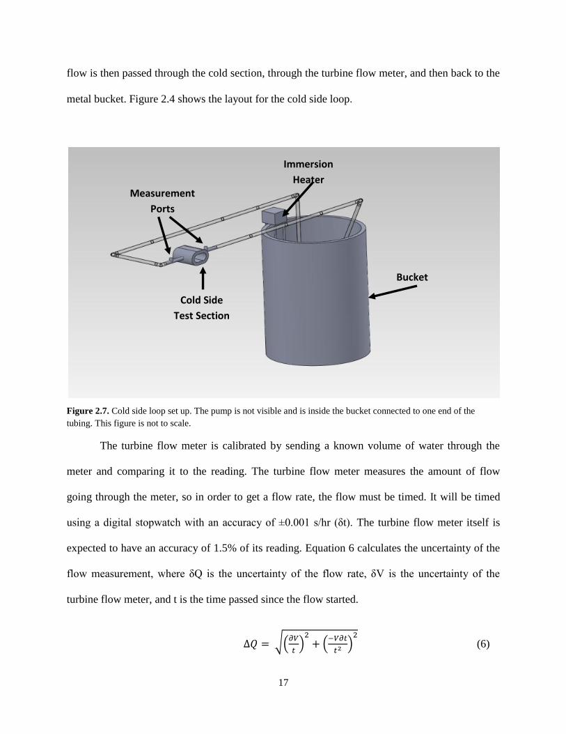
Figure 2.7: Cold side loop set up………………………………………………………….….....17
Figure 2.8: Jitter analysis of the effects of time and volume on the uncertainty of the flow rate
with a constant flow rate considered……………………………………………….…….19
Figure 2.9: Experimental set up…………………………………………………………….…...20
Figure 2.10: Thermocouple placement for both the hot and cold sides of the TEG………….….23
Figure 4.1: Sample flow patterns across the TEG…………………………………………..…..26
Figure 4.2: Layout of TEG material on the test section in the CFD model…………………..…28
vii
Figure 4.3: Comparison of CFD Simulation to the Experimental Data for the Baseline
Geometry…………………………………………………………………………………29
Figure 4.4: Comparison of CFD Simulation to the Experimental Data for the Impingement
Geometry…………………………………………………………………………………32
Figure 4.5: Water flow rate TEG temperature gradient comparison between the baseline and
impingement geometries…………………………………………………………………34
Figure 4.6: Module numbering system………………………………………...……………......35
Figure 4.7: Air flow rate comparison…………………………………………………………....37
Figure 4.8: Air inlet temperature comparison…………………………………………………...38
Table 4.1: Pressure drops across the coolant section geometry…………………….……….….39
viii
NOMENCLATURE
Dh Hydraulic diameter, m
k Thermal conductivity of the material, W/m2K
P Power produced by the thermoelectric generator, W
Pn Pressure measurement, n
Q Heat applied to the thermoelectric generator, W
Re Reynolds Number
Tc Cold side temperature, oC
Th Hot side temperature, oC
T Absolute temperature of the thermoelectric material, oC
t Time passed since the flow through the turbine flow meter began
V Voltage, volts
ZT Figure of Merit of a thermoelectric material
α Seebeck coefficient
ΔT Temperature Difference, oC
ΔP Pressure drop
Pressure drop uncertainty
Uncertainty of the flowrate
Uncertainty of the turbine flow meter

ix
η Efficiency of the thermoelectric generator
μ Dynamic viscosity kg/ms
ρ Electrical resistivity for Equation (2), density for Equation (5)
ν Kinematic viscosity, m2/s

1
CHAPTER 1: INTRODUCTION
In thermoelectric based power generation, the primary research focus has typically involved
improving the properties of the material used in the thermoelectric material. While improving the
material properties could increase the efficiency up to 50% of the stated Carnot efficiency ([1],
[2]), the efficient transfer of heat to/from the TEG is also critical in the overall efficiency of the
thermoelectric (TE) device. The temperature drop across the TE element can be increased by
improving the heat transfer to the hot side of the TEG module and from the cold side using the
coolant flow.
Thermoelectric generation is currently being explored for its power recovery potential in
automobiles. Out of the energy that comes from a combustion process in an engine, 40% is lost
through exhaust gases ([1], [3], and [4]). Thermoelectric generators are intended to capture some
of this otherwise lost energy. Current estimates for the improvement of the fuel economy in a car
using TEG modules are between 2 and 5% [1]. A previous study for this project by Pandit et al.
[5] studied the geometrical effect on heat transfer on the cold side of the TEG module using CFD
models. They predicted that the temperature on the cold side could be reduced to nearly match
that of the coolant temperature. The designed geometries were also aimed at keeping the low
temperatures as evenly distributed as possible and thus lower the overall temperature on the cold
side of the TEG.
This study focuses on the design and testing of an experimental module that aims to improve
the temperature distribution and lower the overall temperature for the cold side and measures
temperature change across the TEG for two cold side geometries. The test stand is designed for a
modular layout, allowing the test section to be easily interchanged between the baseline and

2
impingement geometries. The experiment is 1/5th
scale of the actual heat exchanger module that
will be used in the automobile. The flow rates in the module were scaled down to 1/5th
the
original flow rate. All scaling was based on the Reynolds number of the flow through the full-
size module. The temperatures for the hot side and cold side are typical of engine conditions.
1.1 Thermoelectric systems
The driving technology behind thermoelectric generation is the known as the Seebeck effect.
When a temperature gradient is applied to a thermoelectric material, specifically metals or
semiconductors, the heat passing through is carried by the same particles that carry charge. Once
the heat is removed through the cold side or a heat sink, free electrons are deposited on the cold
side. The movement of charge produces a voltage that can be harnessed and used for other
purposes, such as providing power for minor car electronics. Equation 1 demonstrates how a
temperature gradient affects the voltage, with α as the Seebeck coefficient [3].
(1)
The figure of merit of a material, ZT allows for a quicker comparison of materials suitable
for thermoelectric modules. Equation 2 shows the relation for ZT, which is comprised of the
Seebeck coefficient, the average absolute temperature of the material, T, the electrical resistivity,
ρ, and the thermal conductivity of the material, k. The ideal material has a high Seebeck
coefficient and low electrical resistivity and thermal conductivity.
(2)

3
Because the goal of this project is to put a TEG in a car to recover energy, generated power
from the TEG is an important consideration. Power, P, from a TEG can be calculated using the
efficiency of the TEG, η, and the heat applied to the TEG, Q, as seen in Equation 3.
(3)
The efficiency depends on the temperature difference across the TEG, , the figure of merit,
the hot side temperature, Th, and the cold side temperature, Tc. Equation 4 calculates the
efficiency of the TEG.
√
√ (4)
In order to get the most power generated from the TEG module, a large temperature gradient
is also useful in addition to a high figure of merit for the material. Improving Tc as seen by the
TEG is important as well. A warmer Th increases the temperature gradient, but also effectively
lowers the efficiency. If Tc can be lowered, the temperature gradient still increases without
negatively affecting the efficiency in the denominator of Equation 4. Because the coolant for the
cold side will be derived from the automobile’s existing coolant system, the coolant temperature
is fixed. In order to improve Tc, the next best option is to develop a method to ensure that the
cold side temperature is as close to the coolant temperature as possible. This can be achieved by
improving the heat transfer to the TEG surface using techniques that change the geometry of the
coolant loop, such as fins or impingement holes.

4
1.2 Heat recovery in automobiles
As Yang and Stabler [2] note, of the energy derived from the combustion process within a
car, only 25% of that energy is actually used to put the car in motion and power electrical
accessories within the car. Some of the energy is lost to friction and as heat to the coolant, but
40% is lost to exhaust gas. Even if only 6% of the heat from the exhaust gas could be harnessed,
the TEG could yield a reduction in fuel consumption around 10 percent [7]. Yang and Stabler
also note that the difference of electrical power consumption between typical use of a car and a
car with all optional systems turned off can range between 50 and 1250 W. The amount of
electrical power consumption provides good incentive and opportunity to utilize what is now
currently waste heat and transform it into energy that can be used to power many optional
systems that come with and are frequently used in automobiles today.
1.3 Heat exchangers for TEGs
In order to increase the efficiency of the TEG, two methods can be used. The thermoelectric
material can be made with a higher ZT value, although this is difficult to do and generally the
process in improving the material is costly and time consuming. Another method would be to
improve the temperature gradient across the thermoelectric material. This method is much
simpler and can produce effective results. For each degree Kelvin, the efficiency of the TEG
system can improve up to 0.04% [7]. A type of heat exchanger made to fit around the TEG may
make the necessary improvements in the temperature gradient.
This type of heat exchanger needs to interact with the thermoelectric material for both heat
transfer and stability purposes. The solution includes three main pieces of the system: the
thermoelectric material itself, the hot side loop, and the cold side loop. The hot side loop is an
5
open loop that represents the exhaust pipe. The thermoelectric element lies on a flattened section
of the pipe. Around the hot side and the thermoelectric element, the cold side loop will run,
containing coolant from the car’s existing coolant loop. This study focuses on the improving the
heat transfer from the TE element to the coolant loop, which decreases the temperature of the
cold side of the TEG.
Several different methods of heat exchange were applied to the cold loop in the study
conducted by Pandit et al. [6], including a baseline geometry, a directed flow path, and an
impingement geometry. Out of the three, the baseline and the impingement geometries were
chosen to be tested by this study. The baseline geometry is used as a comparison against future
improvements. The impingement geometry showed the most improvement lowering the
temperatures on the cold side of the TEG in the CFD code. Something that is to be considered in
manufacturing a geometry for the cold side loop is the amount of pressure drop that occurs
across the cold side. Including extraneous features that extrude into the flow are known to
increase the heat transfer at a surface, but the improvements in the heat transfer often come at the
cost of a high pressure drop. Because the coolant loop is derived from the car’s existing coolant
loop, special care must be taken to ensure that the pressure drop caused by the coolant geometry
does not put too much pressure on the coolant pump and strain the coolant system.
1.4 Our Model
The design of the heat exchanger for this study was built around a flattened section of the
exhaust tailpipe. The top and bottom of the pipe are flattened so that pre-manufactured TEGs can
easily and inexpensively be applied. The flattened pipe has more cross sectional area, forcing the
flow to slow down and, as a result, transfer heat more efficiently. The coolant loop built into the
6
car will be extended to wrap around the exhaust pipe and the TEG, providing support for the
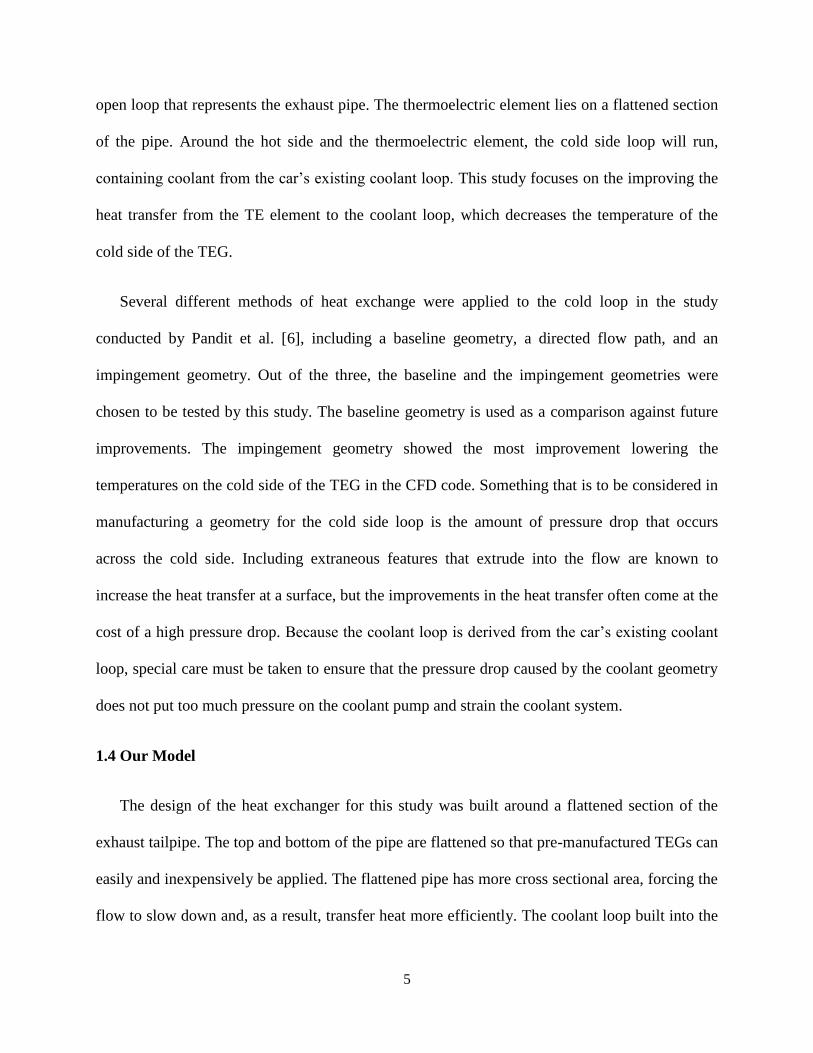
TEG and a method of increasing the temperature gradient across the TEG. Figure 1.1 from
Pandit et al. [5] shows the baseline geometry for the hot and cold sides of the test section. The
brown section is the cold loop test section, which wraps around both the hot loop test section
piece and the TEGs. The gray section is the hot loop test section, and the rectangular pieces
represent the TEG elements. Figure 1.2 shows a front view of the test section and how the TEGs
are placed between the two flow loops. The hot air runs perpendicular to the paper through the
red section. The gray squares represent the TEGs, which are sandwiched in between the hot and
cold sides. The coolant runs around both sets of TEGs through the teal section.
The module for this experiment is scaled down to 1/5th
the size and flow rates of the size
module to be used in an automobile. The scaling is based on the Reynolds number, as seen in
Equation 5. Temperatures were not scaled, so that the full range of temperature gradient
improvement could be observed.
(5)
In the current study, the purpose of the test stand is to improve the temperature gradient
across the TEG module and not to measure the total system energy output. Thus, a scaled down
set-up was acceptable. Using a full-scale model would have been difficult to reproduce the
correct exhaust gas flow rates. As for testing with a used engine, venting exhaust gases in the lab
and maintenance issues were a concern.

7
Figure 1.1. Layout of the baseline heat exchanger. The brown piping is the cold side of the test section, the gray is
the hot side, and the rectangular pieces are sample TEGs. Figure used with permission by Jaideep Pandit, 2012 [5].
Figure 1.2. Front view of the layout of the heat exchanger. The TEG is secured in between the hot and the cold sides
of the heat exchanger.
Cold Side
Hot Side
Cold Side
Hot Side
TE Elements

8
1.5 Literature Survey
There several studies that focused on creating an experimental TEG exhaust system set
up and or improving the heat transfer to the TEG. Some of the previous studies, done by Zorbas
et al. and Chen et al., focused on similar experiments tended to use lower temperatures in the hot
air flow ([8], [9]). There are other studies done by Wojciechowski et al. and Vazquez et al. ([3],
[7]) that use an actual internal combustion engine as the means of heating and moving the gas for
the hot side loop. Vazquez et al. [7] additionally used the coolant system in the engine as the
coolant loop for the cold side of the test section.
There are several different heat exchanger designs that have been tested for effectiveness.
Crane and Lagrandeur [10] changed design geometries from a flat plate design to a cylindrical
hot side that included a bypass exhaust system. Serksnis [11] also used a cylindrical design. Bass
et al [12] used a design that was similar, though it is more hexagonal than cylindrical. The
coolant in this case is applied by a cold plate, held by adjusting screws and springs to keep
tension on the TEG. Many studies choose to use a flat plate design, such as those done by
Birkholz et al. [13], Ikoma et al., [14], Espinosa et al. [15], and Saqr et al. [16]. Ikoma et al. used
two aluminum water cooled jackets to cool the cold side of the TEG, and Saqr et al. used a cold
plate based on a radiator design, using both coolant and the air moving past the vehicle to cool
the TEG.
Saqr et al. gives a comprehensive background on earlier, less efficient thermoelectric
generation designs for automobiles. The article details the capture of recovered power from 1
kW from the work of Bass et al. [12], [17] to 35.6 W through the work of Ikoma et al [14] to 300
W with the work of Thacher et al.[18]. The study done by Saqr et al. draws useful comparisons

9
between the three works through the tables included in the article. Bass et al. achieved a higher
power output, but the group also achieved a higher temperature difference at maximum power
across the thermoelectric element surfaces, at 250oC. Ikoma et al. recorded 123
oC difference, and
Thacher et al. recorded 173.72oC difference. This strongly supports Equations 3 and 4 in the fact
that the higher the temperature gradient is across the TEG, the higher the power output is likely
to be.
Vazquez et al.[7] reviews the works done by Birkholz et al. [13], which was done in
association with Porsche, Serksnis [11],the Nissan Research Center [19,20], and Takanose et al.
[21]. These reviews mostly review the geometries and geometry measurements of the
thermoelectric generators.
1.6 Experimental Objectives
The purpose of this study is to measure the temperature differences across a TEG for
several different running conditions and compare the gradients for two different coolant loop
geometries. This study is compared to a previous study done by Pandit, et al. [5] that models a
full-scale exhaust system and TEG module at similar conditions.
The experiment will be tested at several conditions for each the hot and cold side flow
rates and the inlet hot side temperature. The measured hot side air flow rates are 10, 20, and 25
cfm, and are tested at the inlet temperatures of 200, 300, and 400oC. The cold side water flow
rates are 0.3 and 0.5 gpm.
These conditions are tested at least twice for every combination and each coolant loop
geometry, so that repeatability of the data may be established. Table 1.1 gives a complete list of
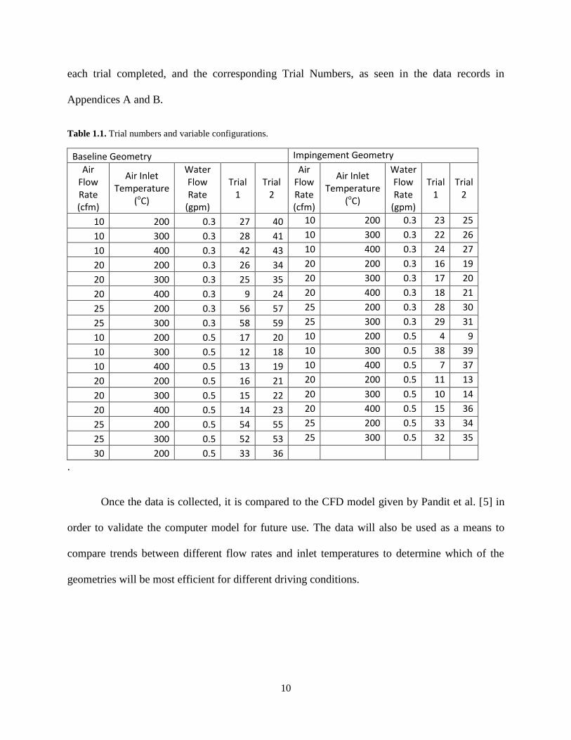
10
each trial completed, and the corresponding Trial Numbers, as seen in the data records in
Appendices A and B.
Table 1.1. Trial numbers and variable configurations.
Baseline Geometry Impingement Geometry
Air Flow Rate (cfm)
Air Inlet Temperature
(oC)
Water Flow Rate
(gpm)
Trial 1
Trial 2
Air Flow Rate (cfm)
Air Inlet Temperature
(oC)
Water Flow Rate
(gpm)
Trial 1
Trial 2
10 200 0.3 27 40 10 200 0.3 23 25
10 300 0.3 28 41 10 300 0.3 22 26
10 400 0.3 42 43 10 400 0.3 24 27
20 200 0.3 26 34 20 200 0.3 16 19
20 300 0.3 25 35 20 300 0.3 17 20
20 400 0.3 9 24 20 400 0.3 18 21
25 200 0.3 56 57 25 200 0.3 28 30
25 300 0.3 58 59 25 300 0.3 29 31
10 200 0.5 17 20 10 200 0.5 4 9
10 300 0.5 12 18 10 300 0.5 38 39
10 400 0.5 13 19 10 400 0.5 7 37
20 200 0.5 16 21 20 200 0.5 11 13
20 300 0.5 15 22 20 300 0.5 10 14
20 400 0.5 14 23 20 400 0.5 15 36
25 200 0.5 54 55 25 200 0.5 33 34
25 300 0.5 52 53 25 300 0.5 32 35
30 200 0.5 33 36
.
Once the data is collected, it is compared to the CFD model given by Pandit et al. [5] in
order to validate the computer model for future use. The data will also be used as a means to
compare trends between different flow rates and inlet temperatures to determine which of the
geometries will be most efficient for different driving conditions.
11
CHAPTER 2: EXPERIMENTAL SETUP
In the current study, the purpose of the test stand is to improve the temperature gradient
across the TEG module. This study does not to measure the total system energy output, thus a
scaled down set-up was acceptable and used. Exhaust gases in the lab and maintenance issues
that may come with a used engine are also no longer a concern with this system. The system is
scaled down to 1/5th
the size that a module being used in an automobile would be, and is scaled
geometrically using the Reynolds Number. Flow rates are also scaled down to 1/5th
the original
rate, but the temperatures remain the same as would be expected in exhaust and coolant flows.
The TEG module has a hot side and a cold side, thus requiring a hot loop and a cold loop.
Typical automobile temperatures are used for the hot and the cold loops. The hot loop in the
CFD model uses 400oC air, based on the temperature of exhaust gas after exiting the catalytic
converter in the tailpipe of a typical sedan ([1], [7]). The coolant loop in the CFD model uses
water at 80oC ([1], [15]). The flow rates in each loop were calculated based on 3000 rpm at 1/5
th
scale of a 3-liter engine. The hot loop has air with a volumetric flow rate of 32 cfm through a
3/8” pipe, and the cold loop runs at 0.5 gpm through 3/8” tubing. In order to quantify changes in
the system, results from the CFD simulation are compared for various heat exchanger
configurations with initial baseline cases. The baseline case is the simplest configuration with no
heat transfer improvement features located in the path of the flow. These baseline measurements
allow us to determine how well the CFD predictions compare with the experimental data before
moving to more complicated designs.
12
2.1 Test Section
The test section was printed in two pieces, the hot and cold sides, using a metal additive
manufacturing process. The pieces were printed using a mix of 420-stainless steel and bronze.
Printing ensures that the details and features of the designed sections were maintained, providing
exactly the same part as the one used in the geometry of the CFD code without the need for
assembly. Figures 2.1 and 2.2 show pictures of the manufactured hot and cold side baseline
geometry sections. The measured roughness of the baseline parts was 1.25 μm Ra on the outside
surfaces and 7.5 μm Ra on the inside surfaces of the part. Because the part is smaller than 7.6 cm
(3”) square, tolerances were quoted to be ±0.13 mm (0.005”).
In order to integrate the parts into the hot and cold loops, steel pipe pieces had to be attached
to the entrances and exits of the test section pieces. Because of the unique make-up of the test
section material, typical welding processes do not work well for the test section. The best
solution for attaching the two pieces is to use a silver solder with a high temperature black flux.
The flux does well for bonding the test section to the steel pipe, and the test section is able to
handle the high temperatures during the experiment.
The two cold side geometries differ on the inside of the section piece, in the flow path. The
baseline geometry is simply a pipe that opens into an open section around the hot side piece, as
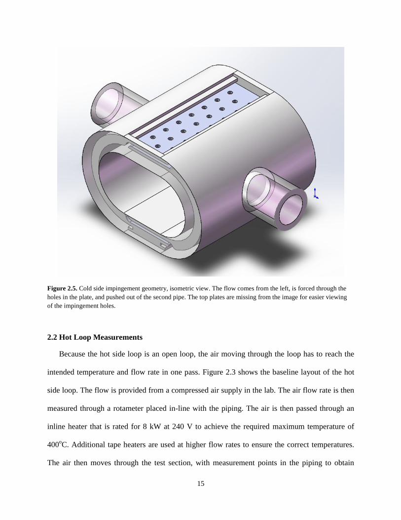
seen in Figure 2.3. The impingement geometry is slightly more complicated. As seen in Figures
2.4 and 2.5, the flow moves in one pipe and it hits a wall on the far side of the flat section of the
cold side. This wall forces the flow through the impingement holes in the flat section. This flow
is pushed out through the second pipe.
13
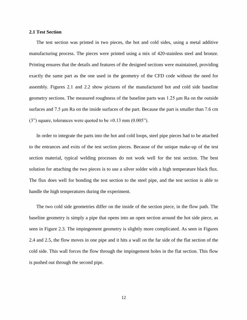
Figure 2.1. Cold side baseline geometry test section piece. This piece is 58 mm x 108 mm x 43 mm.
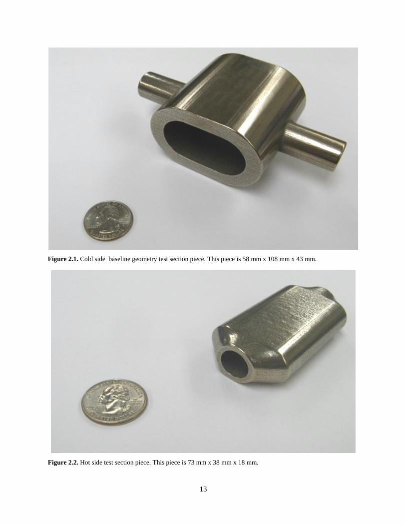
Figure 2.2. Hot side test section piece. This piece is 73 mm x 38 mm x 18 mm.

14
Figure 2.3. Cold side baseline geometry. The pipe opens up, the flow moves around the hot side and back out the
second pipe.
Figure 2.4. Cold side impingement geometry, front view. The flow comes from the left, is forced through the holes
in the plate, and pushed out of the second pipe.
15
Figure 2.5. Cold side impingement geometry, isometric view. The flow comes from the left, is forced through the
holes in the plate, and pushed out of the second pipe. The top plates are missing from the image for easier viewing
of the impingement holes.
2.2 Hot Loop Measurements
Because the hot side loop is an open loop, the air moving through the loop has to reach the
intended temperature and flow rate in one pass. Figure 2.3 shows the baseline layout of the hot
side loop. The flow is provided from a compressed air supply in the lab. The air flow rate is then
measured through a rotameter placed in-line with the piping. The air is then passed through an
inline heater that is rated for 8 kW at 240 V to achieve the required maximum temperature of
400oC. Additional tape heaters are used at higher flow rates to ensure the correct temperatures.
The air then moves through the test section, with measurement points in the piping to obtain
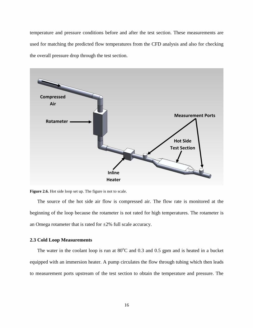
16
temperature and pressure conditions before and after the test section. These measurements are
used for matching the predicted flow temperatures from the CFD analysis and also for checking
the overall pressure drop through the test section.
Figure 2.6. Hot side loop set up. The figure is not to scale.
The source of the hot side air flow is compressed air. The flow rate is monitored at the
beginning of the loop because the rotameter is not rated for high temperatures. The rotameter is
an Omega rotameter that is rated for ±2% full scale accuracy.
2.3 Cold Loop Measurements
The water in the coolant loop is run at 80oC and 0.3 and 0.5 gpm and is heated in a bucket
equipped with an immersion heater. A pump circulates the flow through tubing which then leads
to measurement ports upstream of the test section to obtain the temperature and pressure. The
Compressed
Air
Inline
Heater
Measurement Ports
Hot Side
Test Section
Rotameter
17
flow is then passed through the cold section, through the turbine flow meter, and then back to the
metal bucket. Figure 2.4 shows the layout for the cold side loop.
Figure 2.7. Cold side loop set up. The pump is not visible and is inside the bucket connected to one end of the
tubing. This figure is not to scale.
The turbine flow meter is calibrated by sending a known volume of water through the
meter and comparing it to the reading. The turbine flow meter measures the amount of flow
going through the meter, so in order to get a flow rate, the flow must be timed. It will be timed
using a digital stopwatch with an accuracy of ±0.001 s/hr (δt). The turbine flow meter itself is
expected to have an accuracy of 1.5% of its reading. Equation 6 calculates the uncertainty of the
flow measurement, where δQ is the uncertainty of the flow rate, δV is the uncertainty of the
turbine flow meter, and t is the time passed since the flow started.
√(
)
(
)
(6)
Measurement
Ports
Cold Side
Test Section
Bucket
Immersion
Heater

18
The uncertainty of the flow rate measurement will change depending on the volume of
fluid measured and the amount of time passed. Assuming that the flow stays around the target
flow rate of 0.53 gpm, a jitter analysis can be performed to estimate the uncertainty. Figure 2.5
shows a graph of this analysis. The figures plainly show that as long as the flow runs for a long
enough period of time and enough flow passes through the turbine flow meter, the uncertainty
will stay at a low level of ±0.00795 gpm.
2.4 Overall System Measurements
There are two types of measurements that are made for both the hot and the cold side loops -
pressure drop and temperature from either side of the test sections. Figures 2.3 and 2.4 display
the measurement ports where this data is extracted. Figure 2.6 shows both systems in conjunction
with each other. Hendricks and Krishnan [22] showed a schematic similar to the current layout
for the temperature and pressure measurements. Pressure drop is measured using a dual input
digital manometer over two ports in the flow line. There is one port before the test section and
one after that are used to check the pressure over the test section. The manometer has an
estimated accuracy of ±2% of the full scale. In order to ensure that the temperatures do not
damage the instrument for the hot side, the tubes from the ports to the manometer are connected
using a ball valve. Measurements are taken before the heater for the hot side is started.

19
(a)
(b)
Figure 2.8. Jitter analysis of the effects of time and volume on the uncertainty of the flow rate with a constant flow
rate considered. Plot (a) is the error of the measurement over time, while (b) is the error over the volume passed
through.
0.00794
0.007945
0.00795
0.007955
0.00796
0.007965
0.00797
1 2 3 4 5 6 7 8 9 10 11 12 13 14 15 16 17 18 19 20 21 22 23 24 25
dG
, gp
m
time, t, min
0.00794
0.007945
0.00795
0.007955
0.00796
0.007965
0.00797
0 2 4 6 8 10 12 14
dG
, gp
m
Volume passed, V, gal

20
Figure 2.9. Experimental set up. This is the set up used in the lab to run all of the simulations. The simulated exhaust runs through the heater and the pipes, and
the coolant runs through the clear tubing, perpendicular to the page. The yellow plugs in the picture are the connectors for the thermocouples.
Tape Heaters
Inline Heater
Test Section
Digital Thermometer
Leads for the Cold Side Manometer
Leads for the Hot Side Manometer
Rotameter
Turbine Flow Meter
Stopwatch
Exhaust
Outlet
Cold
Loop
Hot Loop
Water Source,
Heater, and
Pump
21
The uncertainty for the pressure drop is based on Equation 7. Equation 8 shows the how the
uncertainty is to be calculated, where P is the pressure drop uncertainty, ΔP is the pressure
drop, P1 is the first pressure measurement, and P2 is the second pressure measurement. The
company gives the accuracy for the digital manometer to be ±1.5-2%. Assuming the worst
accuracy of 2%, the total maximum uncertainty for the pressure drop is ±2.83%.
(7)
√( ) ( ) (8)
Temperatures are measured using a system of K-type thermocouples and a digital
thermometer. Bare wire thermocouples are used to measure the temperatures at the entrances and
exits of the two loops. The wires plug directly into the digital thermometer, and the temperature
is measured and recorded by hand. The connection port in the digital thermometer allows quick
measurements and easy connection with probes and wires. The digital thermometer is an
acceptable data collection method because the system is measured at steady state.
The temperature distributions across the hot and cold faces of the TEG are the most
important measurement in validating the CFD code. As the scale of the test section is relatively
small, only four temperatures are measured on each side of the TEG, providing a total of 8
temperature measurements. Figure 2.7 shows the locations of the thermocouple probes on the
TEG. K-type probes were chosen for their temperature range, sensitivity, and the fact that they
are commonly available. They generally have a temperature range between -200 and 1250 oC
2
and a sensitivity of 41 µV/ oC [23]. A very small thermocouple probe is needed because the TEG

22
needs to be sandwiched between the hot side and the cold side in order to obtain the highest heat
transfer rate. A 0.5 mm ungrounded probe was chosen. Having an ungrounded probe prevents
ground loops within the metal test section because they are insulated from the sheath wall of the
probe.
The uncertainty for the temperature is determined by the accuracy of the digital thermometer.
The digital thermometer is rated for an accuracy of 1oC plus 0.1% of the reading. The resolution
of the thermometer is 0.1oC.

23
Figure 2.10. Thermocouple placement for both the hot and cold sides of the TEG. The top picture shows the
placement from the front end view of the test section. The bottom picture depicts the placement from a top view.

24
CHAPTER 3: EXPERIMENTAL METHODOLOGY
The experiment requires some set-up before beginning data collection. The water reserve is
heated to 80oC, ±1
oC, and flow is adjusted to 0.3 or 0.5 gpm, ±1gpm, depending on the data
desired. The air for the hot loop is turned on and heated through tape heaters and/or the inline
heater. Once the required temperatures are reached, the system is required to run for at least
twenty minutes before data collection to ensure the TEG has become acclimated to the system
temperatures, and steady state has been achieved.
Water and air temperature and flow rate measurements are checked once more before data is
collected. These initial conditions are recorded. Once everything has been determined to be
steady and at the correct parameters for the experiment, temperatures are taken through the
digital thermometer and recorded by hand. Pressure drop for the coolant loop is measured by the
digital manometer and recorded. Because the air temperatures are too hot for the tubing and the
manometer to handle, air pressure drops are recorded when the heaters are not running.
The data is recorded in a master excel sheet, as seen in Appendices A and B. Data for each
set of conditions is taken at least twice to be checked for repeatability. The data is considered
repeatable if the temperatures of across the hot and cold sides of the TEG and the differences for
each of the respective thermocouple probes are within eleven degrees of each other.
Several factors need to be checked while experimenting. Water within the reservoir needs to
stay at a certain level to ensure that the immersion heater is covered and will not burn out. Water
temperature and flow rate need to be checked and adjusted often. Close attention to the rotameter
should be paid to ensure that the air flow rate has not dropped. Thermocouple probes should be

25
checked to ensure that they are still in the correct locations for measurement and reattached to
the TEG if necessary.

26
CHAPTER 4: RESULTS
4.1 TEG Model Layout and Flow Overview
In order to better understand the distribution of the temperatures, it is useful to
understand how the flows are moving across the TEG. The exhaust and coolant flows move
perpendicular to each other across the TEG, as seen in Figure 4.1. The figure demonstrates how
the flow movements affect the temperature gradients across the TEG. This sample was
extrapolated from the four temperature measurements across the surface of the TEG, so this
contour plot is only a representation of the temperatures. It can be seen that the temperature
differences are highest where the exhaust gas first comes into contact with the TEG and when the
coolant flow comes into contact with the TEG, and lower near the exit boundaries. These
patterns are important to keep in mind as comparison plots for the CFD simulation, the baseline
experiments, and the impingement experiments are shown.
Figure 4.1. Sample flow patterns across the TEG. This pattern is extracted from the four sample points from the
temperature difference between the hot side and the cold side of the TEG. Representation only.

27
4.2 CFD Simulation and Experimental Results Comparison and Validation
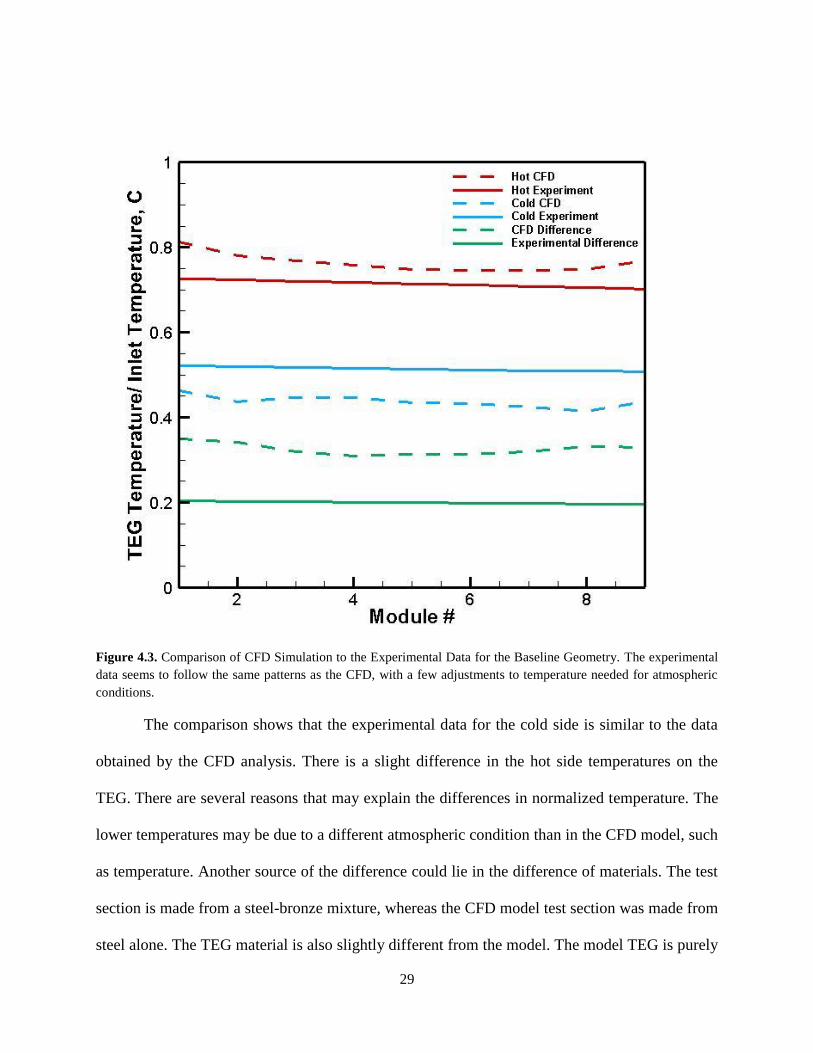
4.2.1 Baseline CFD Comparison
One of the major components of this study is to compare the results of the CFD
simulation done by Pandit et al [5] with experimental results. The Baseline geometry simulation
conducted by Pandit at 400 o
C, 0.5 gpm, and 30 cfm was compared to a 200 o
C 0.5 gpm, 30 cfm
Baseline geometry experimental case. The case was completed using 200 o
C inlet air instead of
400oC because of limitations with the heaters at that high of a flow rate. This is compensated for
by normalizing the temperatures across the TEG with the inlet temperature of the case. For
example, if a temperature on the TEG was 303 o
C in the CFD simulation, it was divided by the
inlet temperature 400 oC for normalization. An experimental value was normalized by 200
oC.
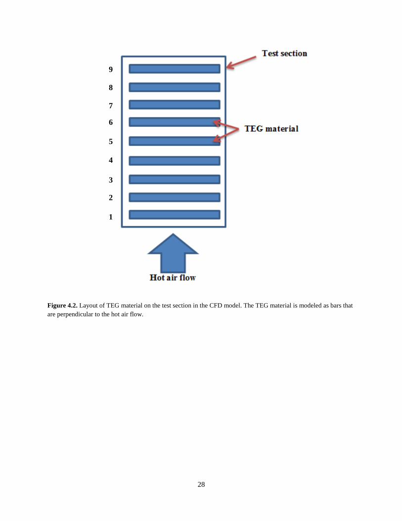
The TEG layout for the CFD model consists of nine different bars that lay perpendicular
to the direction of the hot air flow. Figure 4.2 demonstrates the layout of the TEG elements in the
CFD model. Temperatures are averaged along these bars and plotted on Figure 4.3. The
thermocouple measurements consist of two averaged measurements that are parallel to the
direction of the flow. The two measurements predict a trend of temperatures along the flow
direction for comparison purposes.
28
Figure 4.2. Layout of TEG material on the test section in the CFD model. The TEG material is modeled as bars that
are perpendicular to the hot air flow.
1
2
3
4
5
6
7
8
9
29
Figure 4.3. Comparison of CFD Simulation to the Experimental Data for the Baseline Geometry. The experimental
data seems to follow the same patterns as the CFD, with a few adjustments to temperature needed for atmospheric
conditions.
The comparison shows that the experimental data for the cold side is similar to the data
obtained by the CFD analysis. There is a slight difference in the hot side temperatures on the
TEG. There are several reasons that may explain the differences in normalized temperature. The
lower temperatures may be due to a different atmospheric condition than in the CFD model, such
as temperature. Another source of the difference could lie in the difference of materials. The test
section is made from a steel-bronze mixture, whereas the CFD model test section was made from
steel alone. The TEG material is also slightly different from the model. The model TEG is purely

30
bismuth-telluride, wheras the experimental TEG has layers of graphite, aluminum, and adhesives
that were previously unaccounted for. Geometry may have also had an effect on the results. The
test section modeled in the CFD simulation was scaled down to be the blueprint for the
experiment test section. One thing that couldn’t be scaled, however, was the wall thickness of the
test piece. This may have affected the conduction from the fluid to the TEG.
4.2.2 Impingement CFD Comparison
It is also important to compare the CFD simulation to the experimental results for the
impingement case. In this case, the CFD simulation ran with 400oC air at 30 cfm, and the water
was run at 0.5 gpm. In the experimental data runs, the one of the closest cases for comparison
available was 200oC air at 25 cfm, where the water was pumped at 0.5 gpm. In order to account
for these changes in the data, the temperature on the TEG was normalized by the inlet air
temperature, as was done for the baseline geometry, and multiplied by the Reynolds number the
simulation or experiment was based on. The corresponding air flow rate was calculated for each
Reynolds number. Figure 4.4 plots the data comparison between the experiment and the CFD
simulation.
The experimental data follows similar patterns as the CFD simulation data does, but there
are vastly different temperature ranges between the two. There are several different reasons for
this. First, as with the baseline geometry, some of the environmental conditions varied from the
experimental set up. In the CFD simulation, the test module was treated as insulated, but the
experiment was open to the atmosphere. There also may have been a temperature variance
between the CFD atmosphere temperature and the actual temperature in the lab surrounding the
test set up.
31
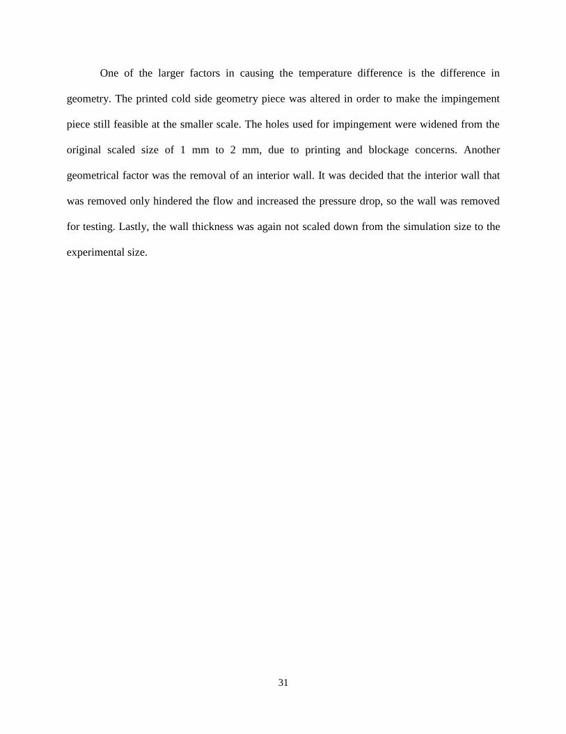
One of the larger factors in causing the temperature difference is the difference in
geometry. The printed cold side geometry piece was altered in order to make the impingement
piece still feasible at the smaller scale. The holes used for impingement were widened from the
original scaled size of 1 mm to 2 mm, due to printing and blockage concerns. Another
geometrical factor was the removal of an interior wall. It was decided that the interior wall that
was removed only hindered the flow and increased the pressure drop, so the wall was removed
for testing. Lastly, the wall thickness was again not scaled down from the simulation size to the
experimental size.
32
Figure 4.4. Comparison of CFD Simulation to the Experimental Data for the Impingement Geometry. The
experimental data seems to follow similar patterns as the CFD, but the temperatures vary wildly due experimental
differences.
4.3 Baseline Geometry vs. Impingement Geometry Comparison
In testing the two geometries, there were three variables that were adjusted to find the
most optimal environment for obtaining a higher temperature gradient: water flow rate, air flow
rate, and air inlet temperature. In the following sections, each of these variables were studied for
their effect on the temperature gradient for each the baseline geometry and the impingement
geometry.
33
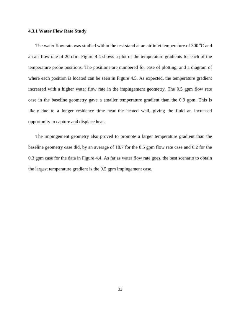
4.3.1 Water Flow Rate Study
The water flow rate was studied within the test stand at an air inlet temperature of 300 o
C and
an air flow rate of 20 cfm. Figure 4.4 shows a plot of the temperature gradients for each of the
temperature probe positions. The positions are numbered for ease of plotting, and a diagram of
where each position is located can be seen in Figure 4.5. As expected, the temperature gradient
increased with a higher water flow rate in the impingement geometry. The 0.5 gpm flow rate
case in the baseline geometry gave a smaller temperature gradient than the 0.3 gpm. This is
likely due to a longer residence time near the heated wall, giving the fluid an increased
opportunity to capture and displace heat.
The impingement geometry also proved to promote a larger temperature gradient than the
baseline geometry case did, by an average of 18.7 for the 0.5 gpm flow rate case and 6.2 for the
0.3 gpm case for the data in Figure 4.4. As far as water flow rate goes, the best scenario to obtain
the largest temperature gradient is the 0.5 gpm impingement case.

34
Figure 4.5. Water flow rate TEG temperature gradient comparison between the baseline and impingement
geometries. The air flow was set to run at 300 o
C and 20 cfm. The gradient generally increases with increased flow
rate and the use of the impingement geometry.
35
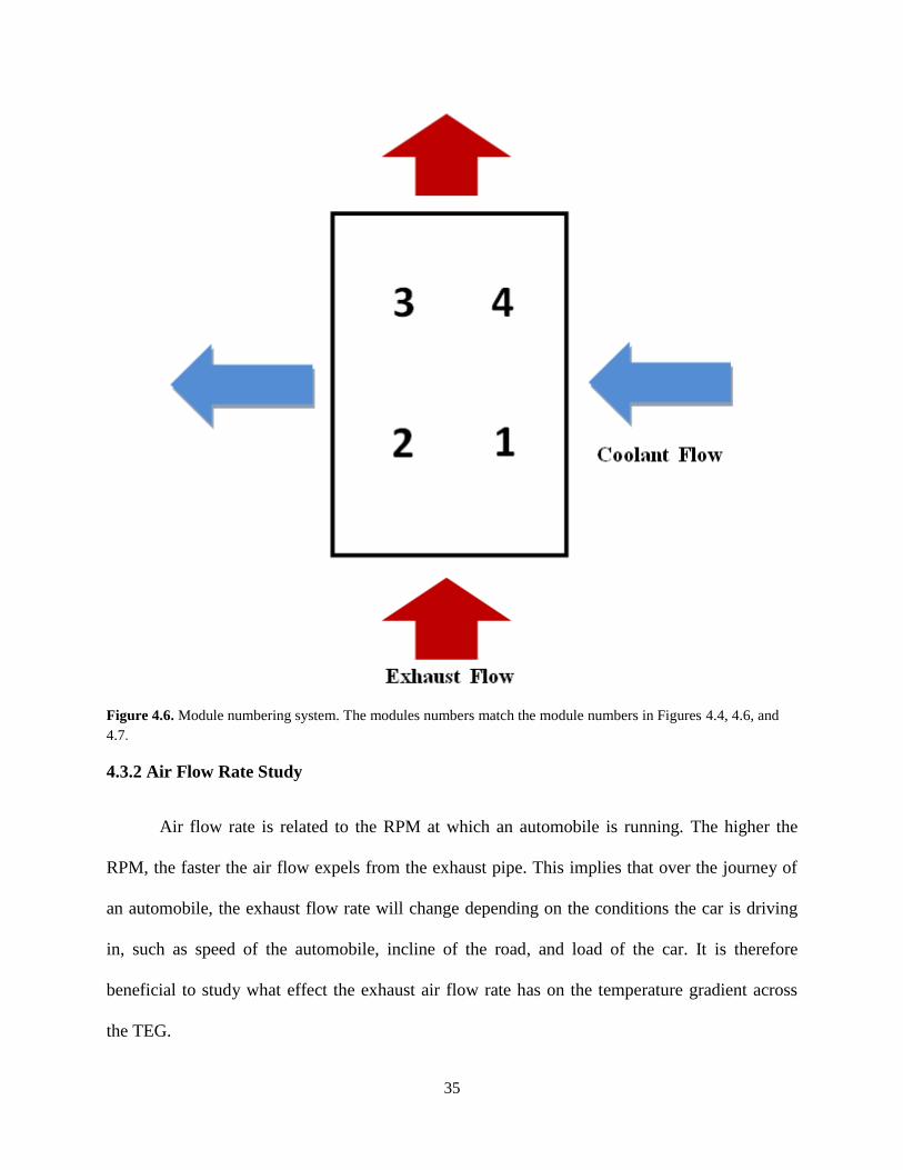
Figure 4.6. Module numbering system. The modules numbers match the module numbers in Figures 4.4, 4.6, and
4.7.
4.3.2 Air Flow Rate Study
Air flow rate is related to the RPM at which an automobile is running. The higher the
RPM, the faster the air flow expels from the exhaust pipe. This implies that over the journey of
an automobile, the exhaust flow rate will change depending on the conditions the car is driving
in, such as speed of the automobile, incline of the road, and load of the car. It is therefore
beneficial to study what effect the exhaust air flow rate has on the temperature gradient across
the TEG.
36
The experiment was run at three different air flow rates for both the baseline and
impingement geometries: 10 cfm, 20 cfm, and 25 cfm. While the CFD simulation modeled data
at 30 cfm, it was not possible with the current heaters in the set up to obtain useful temperatures
at 30 cfm. Figure 4.6 plots the temperature differences for each of these flow rates for both
geometries. As expected, the temperature gradient increased with higher air flow rates. Because
the tests are currently being run with a baseline hot side section, the difference between the cold
side baseline and the impingement geometry temperature gradients comes from the difference
the geometries make on the cold side of the TEG. Comparing the two geometries, there is a
6.7oC increase in temperature gradient at 10 cfm, a 6.2
oC increase for 20 cfm, and a 7.6
oC
increase for 25 cfm in this case. The gradient increases 9.0 o
C between 10 and 20 cfm for the
impingement and 10.5 oC between 10 and 25 cfm for the impingement case

37
Figure 4.7. Air flow rate comparison. Temperature gradient increases with increasing exhaust air flow rate. Baseline
and impingement temperature effects are comparable, as the difference in the gradient temperatures here are derived
from the cold side of the TEG.
4.3.3 Air Inlet Temperature Study
As with the exhaust air flow rate, the temperature of the exhaust depends on the RPM of
the automobile. Figure 4.7 is a plot of the temperature gradients for inlet temperatures of 200oC,
300oC, and 300
oC for both the baseline and impingement geometry cases. These cases behave

38
exactly as predicted. Increasing the inlet temperature of the exhaust air increases the temperature
on the hot side of the TEG, which increases the temperature gradient. The gradients for this case
increase by 39.7 o
C for the impingement piece between the 200 o
C and 300 o
C cases, and 73.8 o
C
for the impingement piece between the 200 o
C and 400 o
C cases. Impingement gradients are
consistently larger than the baseline gradients due to the fact that the hot side geometry does not
change between the cold side impingement and baseline geometries.
Figure 4.8. Air inlet temperature comparison. Temperature gradient increases with increased inlet temperature,
steadily for both the baseline and the impingement geometries.
39
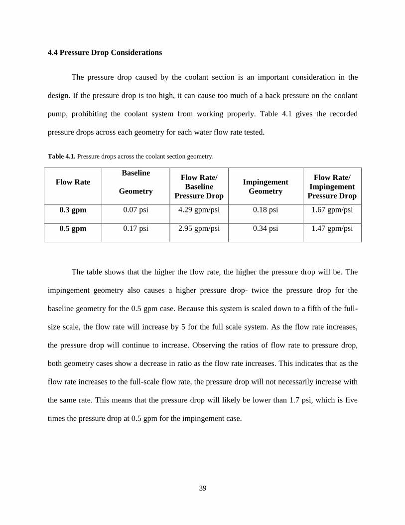
4.4 Pressure Drop Considerations
The pressure drop caused by the coolant section is an important consideration in the
design. If the pressure drop is too high, it can cause too much of a back pressure on the coolant
pump, prohibiting the coolant system from working properly. Table 4.1 gives the recorded
pressure drops across each geometry for each water flow rate tested.
Table 4.1. Pressure drops across the coolant section geometry.
Flow Rate
Baseline
Geometry
Flow Rate/
Baseline
Pressure Drop
Impingement
Geometry
Flow Rate/
Impingement
Pressure Drop
0.3 gpm 0.07 psi 4.29 gpm/psi 0.18 psi 1.67 gpm/psi
0.5 gpm 0.17 psi 2.95 gpm/psi 0.34 psi 1.47 gpm/psi
The table shows that the higher the flow rate, the higher the pressure drop will be. The
impingement geometry also causes a higher pressure drop- twice the pressure drop for the
baseline geometry for the 0.5 gpm case. Because this system is scaled down to a fifth of the full-
size scale, the flow rate will increase by 5 for the full scale system. As the flow rate increases,
the pressure drop will continue to increase. Observing the ratios of flow rate to pressure drop,
both geometry cases show a decrease in ratio as the flow rate increases. This indicates that as the
flow rate increases to the full-scale flow rate, the pressure drop will not necessarily increase with
the same rate. This means that the pressure drop will likely be lower than 1.7 psi, which is five
times the pressure drop at 0.5 gpm for the impingement case.
40
CHAPTER 5: SUMMARY AND CONCLUSIONS
A new test loop has been designed and developed for testing using a steady-state method to
obtain temperature, pressure, and flow measurements inside a thermoelectric generator system.
The test loop allows for variability of the heat exchanger module, TEG material, and variability
of flow parameters. The current set up is modular and allows the user to easily change the test
sections, in order to test different heat exchanger geometries and change parts as needed. The
results obtained from this experimental setup are used to validate baseline and impingement CFD
models.
The CFD simulations will compare reasonably with the experimental values, once small
adjustments are made. For the baseline case, the trends are very similar for the simulation and the
experiment, but there are differences in gradient values due to differences in simulation boundary
conditions. For the impingement case, the trends are again similar, but the temperatures predicted
by the CFD code are much different than the experimental values. With a few adjustments to the
models, the CFD simulations could be a good predictor of the temperature differences across the
TE element. Geometries specifically need to be updated, as do the environmental conditions
surrounding the test module.
Through the operation of this unit in an automobile, many different conditions will affect the
performance of the TEG through the cold side of the thermoelectric material. Depending on
coolant pump conditions, the water flow rate may vary. Out of the conditions tested, it appears
that the impingement geometry will produce the larger temperature gradient resulting from a
flow rate of 0.5 gpm. In the baseline case, 0.3 gpm produced a higher temperature gradient. The
air flow rates indicate that the higher the flow rate, the larger the temperature gradient will be.
41
Because this parameter pertains to the hot side flow, changing the cold side geometry does not
have a noticeable effect on the temperature. The temperature gradient is slightly higher in the
impingement geometry, but this is due to the cold side counterpart decreasing in temperature
gradient. The air inlet temperature also affects the temperature gradient. The higher the
temperature entering the hot side of the test section, the larger the temperature gradient will be.
Again, because this parameter applies to the hot side, the temperature difference affected by this
parameter will not vary much between the baseline and impingement geometry cases. In each
condition tested, the impingement gives a greater temperature gradient than the baseline case.
Based on the data presented in this paper, it appears that the impingement has improved the
temperature distribution by roughly 10 degrees over the baseline geometry.
The pressure drop across coolant geometry is highest for larger flow rates and the
impingement geometry. For a full-sized thermoelectric generator, the flow rates and resulting
pressure drops will increase. Based on the current trends of pressure drop versus increased flow
rate, the pressure drop is not likely to exceed 1.7 psi.
This study focuses on fabricating a modulated test stand and understanding which parameters
will favorably increase the temperature gradient across the thermoelectric element. This study is
an important step in expanding knowledge further for hot side temperature measurements,
validating CFD models, and demonstrating the better design of the impingement flow geometry
for the cold side test section piece.

42
REFERENCES
1. Yang, J. and Caillat, T. 2006. “Thermoelectric Materials for Space and Automotive Power
Generation.” MRS Bull. 31. pp 224-229.
2. Yang, J. and Stabler, F. 2009. “Automotive Applications of Thermoelectric Materials.”
Journal of Electronic Materials, 38, (7).
3. Wojciechowski, K., Merkisz, J., Fuc P., Lijewski, P. Schmidt, M. 2007. “Study of Recovery
of Waste Heat from the Exhaust of Automotive Engine.” Proc., 5th
European Conference on
Thermoelectrics. Odessa, Ukraine.
4. Yang, J. 2005. “Potential Applications of Thermoelectric Waste Heat Recovery in the
Automotive Industry.” Proc. 24th
Int. Conf. Thermoelectrics. Clemson University, United
States. IEEE, 155-160.
5. Pandit, J., Dove, M., Ekkad, S., and Huxtable, S. 2012. “Heat Exchanger Design for Waste
Heat Recovery from Automobile Exhaust Using Thermoelectric Generators.” Proc., 50th
AIAA Aerospace Sciences Meeting. Nashville, Tennessee.
6. Snyder, G. J. 2008. “Thermoelectric Energy Harvesting.” Chapter 11 in “Energy Harvesting
Technologies,” S. Priya &D. Inman, Eds pg 329.
7. Vazquez, J., Sanz-Bobi, M., Palacios, R. Arenas, A. 2002. “State of the Art Thermoelectric
Generators Based on Heat Recovered from the Exhaust Gases of Automobiles.” Proc., 7th
European Workshop on Thermoelectrics. Pamplona, Spain, Paper # 17.
8. Zorbas, K. T., Hatzikraniotis, E. Paraskevopoulos, K. M. 2007. “Power and Efficiency
Calculation in Commercial TEG and Application in Wasted Heat Recovery in Automobile.”
Proc., 5th
European Conference on Thermoelectrics. Odessa, Ukraine, Paper #30.
43
9. Chen, M. Andreasen, S., Rosendahl, L., Kaer, S. K., Condra, T. 2010. “System Modeling and
validation of a Thermoelectric Fluidic Power Source: Proton Exchange Membrane Fuel Cell
and Thermoelectric Generator.” Journal of Electronic materials, 39 (9). pp 1593-1600.
10. Crane, D. and LaGrandeur, J. 2010 “Progress Report on BSST-Led US Department of
Energy Automotive Waste Heat Recovery Program.” Journal of Electronic Materials. 39 (9).
pp 2142-2148.
11. Serksnis, A.W. Thermoelectric Generator of Automotive Charging System. 1976. Prox. 11th
Intersociety Conversion Engineering Conference. New York, USA, pp. 1614-1618.
12. Bass, J., Campana, R.J., and Elsner, N.B. 1992. “Thermoelectric generator development for
heavy-duty truck applications.” Proc. Annual Automotive Technology Development
Contractors Coordination Meeting, Dearborn, USA, pp 743-748.
13. Birkholz, U., et al. 1988. “Conversion of Waste Exhaust Heat in Automobile using FeSi2
Thermoelements.” Proc. 7th
International Conference of Thermoelectric Energy Conversion.
Arlington, USA, pp. 124-128.
14. Ikoma, K., et al. 1998. “Thermoelectric Module and Generator for Gasoline Engine
Vehicles.” Proc. 17th
International Conference on Thermoelectrics. Nagoya, Japan, pp. 464-
467.
15. Espinosa, N., Lazard, M., Aixala, L., Scherrer, H. 2010. “Modeling a Thermoelectric
Generator Applied to Diesel Automotive Heat Recovery.” Journal of Electronic materials,
39 (9). pp 1446-1455.
16. Saqr, K.M., Mansour, M.K., Musa, M.N. 2008. “Thermal Design of Automobile Exhaust
Based Thermoelectric Generators: Objectives and Challenges.” International Journal of
Automotive Technology, 9 (2), pp. 155-160.
44
17. Bass, J., Elsner, N.B., and Leavitt, A. 1995. “Performance of the 1 kW Thermoelectric
Generator for Diesel Engines.” Proc. 13th
Int. Conf. Thermoelectrics B, Mathiprakisam, edn.,
AIP Conf. Proc., New York, p 295.
18. Thacher, E.F., Helenbrook, B.T., Karri, M.A., and Richter, C.J. 2007. “Testing of an
Automobile Exhaust Thermoelectric Generator in a Light Truck.” Proc. I MECH E, Part D:
J. Automobile Engineering. 221, 1, 95-107.
19. Shinohara, K., et al. 1999. “Application of Thermoelectric Generator for Automobiles.”
Journal of the Japan Society of Power and Power Metallurgy, 46 (5), pp. 524-528.
20. Ikoma, K., et al. 1999. “Thermoelectric Generator for Gasoline Engine Vehicles Using
Bi2Te3 Modules.” J. Japan Inst. Metals. Special Issue on Thermoelectric Energy Conversion
Materials, 63 (11), pp. 1475-1478.
21. Takanose, E. and Tamakoshi, H. 1993. “The Development of Thermoelectric Generator for
Passenger Car.” Proc. 12th
International Conference on Thermoelectrics. Yokohama, Japan,
pp. 467-470.
22. Hendricks, T. and Krishnan, S. 2012. “Micro- & Nano- Technologies Enabling More
Compact, Lightweight Thermoelectric Power Generation & Cooling Systems.” 3rd
Thermoelectric Applications Workshop. Baltimore, Maryland.
23. ”Practical Thermocouple Temperature Measurements”, Dataforth Corporation,
http://www.dataforth.com/catalog/pdf/an107.pdf, downloaded March 2012.

45
APPENDIX A- BASELINE GEOMETRY DATA
Run 1 Run 2 Run 3 Run 4 Run 5 Run 6 Run 7 Run 8 Run 9 Run 10
Hot Side
Air flow rate (cfm) 27 27 28 28 10 8 10 10 20 10
Inlet temperature (C) 331 338 297 305 200 300 300 400 400 200
Outlet temperature (C) 276 281 250 254 156 228 231 303 323 156
Pressure Drop (inH2O)
48.8 48.8 22.6 5.1 8.1 8.1 27
Cold Side
Water flow rate (gpm) 0.38 0.4 0.5 0.3 0.3 0.3 0.3 0.3 0.3 0.53
Inlet temperature (C) 79.5 83 79.2 79.9 79.5 80 80 80.4 80.2 79.6
Outlet temperature (C) 78.5 82.7 80 80.2 79.2 79.8 79.8 80.5 80.5 79.4
Pressure Drop (inH2O) 7.4 7.5 8.6 5.5 2.04 2.04 2.04 2.06 2.16 7.5
Test Section (C)
TFL 152.5 154 119.5 136.2 109 137.5 138.3 173.9 177.4 105.7
BFL 218 224 196.7 215 135.7 190.7 192.5 251 274 133.6
Temperature drop 65.5 70 77.2 78.8 26.7 53.2 54.2 77.1 96.6 27.9
TBL 154.8 158.2 130.1 126.8 103.7 125.8 126.2 160 180.8 100
BBL 226 235 209 209 131.4 180.1 183.2 236 249 130.4
Temperature drop 71.2 76.8 78.9 82.2 27.7 54.3 57 76 68.2 30.4
TFR 143.3 143 115.5 125 105.5 127.1 125.2 157.2 156.9 113.1
BFR 223 232 175.3 197 135.4 185.5 186.3 243 263 135.5
Temperature drop 79.7 89 59.8 72 29.9 58.4 61.1 85.8 106.1 22.4
TBR 170.5 167.6 -- -- 105.2 132.4 135 169.4 164 98.9
BBR 243 246 213 213 138 190.4 192.4 249 260 130.2
Temperature drop 72.5 78.4
32.8 58 57.4 79.6 96 31.3
Steady State?
46
air dP 10 20 25 30 cfm in H2O 3.95 20.5 33.5 48.8 Run 11 Run 12 Run 13 Run 14 Run 15 Run 16 Run 17 Run 18 Run 19 Run 20 Run 21 Run 22 Run 23
10 10 10 20 20 20 10 10 10 10 20 20 20
300 300 400 400 300 200 200 300 400 200 200 300 400
228 230 303 323 245 166.7 156.4 231 301 156.4 165.8 245 322
0.5 0.52 0.52 0.52 0.5 0.52 0.5 0.5 0.52 0.51 0.51 0.5 0.5
79.4 79.8 79.9 79.9 79.5 79.5 79.5 79.1 79.8 80.3 80.9 80.2 80
79.3 79.4 80 80.1 79.6 79.3 79.3 79.1 79.9 80.1 80.8 80.3 79.9
7.5
7.9
7.5 7.7 7.5 7
7.5 6.6
129.5 131.7 146.6 154.9 132.4 104.6 101.9 124 145.9 107.2 110.8 138 165.6
189.1 180.5 232 248 191.6 135.6 131.4 178.4 228 132.9 141 198.1 256
59.6 48.8 85.4 93.1 59.2 31 29.5 54.4 82.1 25.7 30.2 60.1 90.4
120.1 129.9 143.3 148.8 122.7 102.3 99.9 119.1 139.1 96.5 98.9 116.8 143.3
179.6 184.7 237 256 194.3 137.6 131.5 182.4 237 126.3 132.9 184.4 251
59.5 54.8 93.7 107.2 71.6 35.3 31.6 63.3 97.9 29.8 34 67.6 107.7
145.2 120.8 144.7 153.4 126.9 103.8 101 122.3 142.8 108.3 111.1 136.2 163.8
186.9 182.7 238 255 197 139.7 132.8 183 235 126.9 133.5 182 248
41.7 61.9 93.3 101.6 70.1 35.9 31.8 60.7 92.2 18.6 22.4 45.8 84.2
116.9 117.7 136.9 141.6 118 99.6 97.5 114.4 132.3 98.3 100.3 117.1 145.1
179.4 186.4 235 252 192.8 137.4 132.3 183.7 235 121.3 126.8 170.7 230
62.5 68.7 98.1 110.4 74.8 37.8 34.8 69.3 102.7 23 26.5 53.6 84.9
47
Run 24 Run 25 Run 26 Run 27 Run 28 Run 29 Run 30 Run 31 Run 32 Run 33 Run 34 Run 35 Run 36
20 20 20 10 10 10 30 30 30 30 20 20 30
400 300 200 200 300 400 200 300 200 200 200 300 200
321 244 165.9 156.4 230 301 167.7 248 169 169.7 165.5 243 169.5
0.3 0.3 0.3 0.3 0.3 0.31 0.3 0.3 0.3 0.5 0.3 0.3 0.5
80.6 79.8 79.3 80.1 79.9 79 80.5 79.8 79.4 80.2 79.4 80.1 79.7
80.8 79.9 79.2 79.4 79.5 79 80.5 79.6 79.2 80.1 79.1 80 79.7
9.1 9.4 6.4 5.5 5.5 5.7 5.3 5.5
7.2 5.3 5.5 9
157.5 126.3 104.1 101.8 122.1 143.2 105 128.2 104.8 104.6 102.9 124.9 103.6
259 198.5 140.1 133.3 186.1 235 143 203 144.3 144.5 140 197.3 143.8
101.5 72.2 36 31.5 64 91.8 38 74.8 39.5 39.9 37.1 72.4 40.2
134.9 115.2 97.9 95.9 113.1 141.5 101.7 121.5 101.3 102 100 119.7 100.2
245 187.4 134.8 128.8 178.9 239 141.2 199.1 141.5 141.5 136.7 192.9 140.3
110.1 72.2 36.9 32.9 65.8 97.5 39.5 77.6 40.2 39.5 36.7 73.2 40.1
147.2 122.8 102.9 101.4 121.2 136.4 104.1 125.8 104.1 104 102.4 123.5 103.2
252 193.2 139.2 131.7 182.5 241 141.1 204 145.9 145.8 141 197.4 144.1
104.8 70.4 36.3 30.3 61.3 104.6 37 78.2 41.8 41.8 38.6 73.9 40.9
136.3 116.1 98.3 97.4 114.4 130.2 101.1 120.3 100.4 100.7 98.6 117.3 99.4
244 176.3 140.1 124.7 169.3 235 138.4 192 139.2 139.4 134.8 186.2 137.7
107.7 60.2 41.8 27.3 54.9 104.8 37.3 71.7 38.8 38.7 36.2 68.9 38.3
*air flow may have been low

48
Run 37 Run 38 Run 39 Run 40 Run 41 Run 42 Run 43 Run 44 Run 45 Run 46 Run 47 Run 48 Run 49
10 10 10 10 10 10 10 20 10 20 20 20 10
200 300 400 200 300 400 400 400 400 200 300 300 200
143.1 253 156.2 229 299 300 321 299 164.4 242 243 155.8
0.3 0.29 0.3 0.306 0.3 0.3 0.3 0.3 0.5 0.5 0.5 0.5 0.5
80.7 80.2 80.9 80.5 80.5 80.2 80.2 80.4 79.8 79.3 79.2 79.2 79.1
80.2 79.9 80.8 80.2 80.6 80.4 80.4 80.4 79.8 79.1 79 79 78.8
~1 ~0.5 ~0.5 ~0.7
97.3 114.1 130.7 101 121 141 140.3 148.8 139 101.8 123.8 123.4 102.2
124.3 164.9 206 131.5 183.3 238 237 259 237 140.2 197.9 197.3 126.7
27 50.8 75.3 30.5 62.3 97 96.7 110.2 98 38.4 74.1 73.9 24.5
94.5 108.6 124 96.8 113.2 132.7 131.7 138.4 129.7 97 114.8 113.9 101
121 159.7 199 128.6 177 230 230 249 230 135.4 189.4 185.5 130.8
26.5 51.1 75 31.8 63.8 97.3 98.3 110.6 100.3 38.4 74.6 71.6 29.8
97.5 114.4 130.8 101.8 122.6 143.5 143 151.6 141.5 103.1 125.5 126.4 101.9
123.7 165.5 206 130.9 181.1 235 235 255 232 138.3 195.1 189.5 131.9
26.2 51.1 75.2 29.1 58.5 91.5 92 103.4 90.5 35.2 69.6 63.1 30
95 108.3 123.3 97.9 114.9 132.7 132.1 138.9 130.9 97.9 116.3 115.5 99.1
118.7 155.1 191.3 125.6 171 221 220 237 219 131.4 180.5 177.3 130.7
23.7 46.8 68 27.7 56.1 88.3 87.9 98.1 88.1 33.5 64.2 61.8 31.6
*taken with t type setting
49
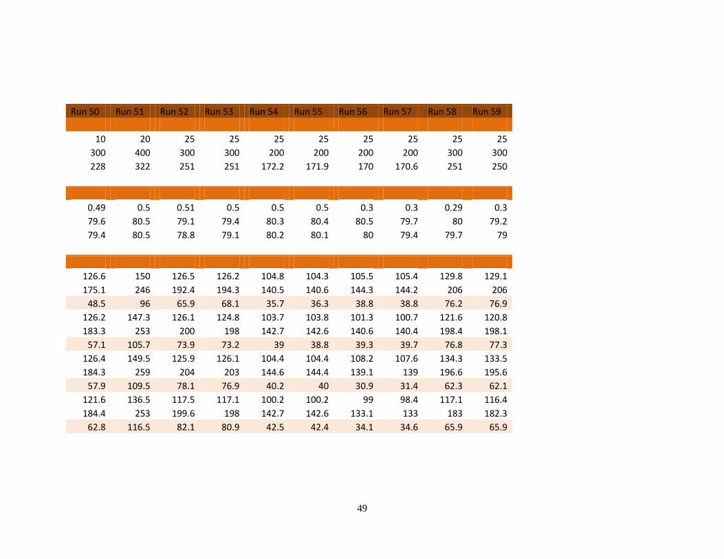
Run 50 Run 51 Run 52 Run 53 Run 54 Run 55 Run 56 Run 57 Run 58 Run 59
10 20 25 25 25 25 25 25 25 25
300 400 300 300 200 200 200 200 300 300
228 322 251 251 172.2 171.9 170 170.6 251 250
0.49 0.5 0.51 0.5 0.5 0.5 0.3 0.3 0.29 0.3
79.6 80.5 79.1 79.4 80.3 80.4 80.5 79.7 80 79.2
79.4 80.5 78.8 79.1 80.2 80.1 80 79.4 79.7 79
126.6 150 126.5 126.2 104.8 104.3 105.5 105.4 129.8 129.1
175.1 246 192.4 194.3 140.5 140.6 144.3 144.2 206 206
48.5 96 65.9 68.1 35.7 36.3 38.8 38.8 76.2 76.9
126.2 147.3 126.1 124.8 103.7 103.8 101.3 100.7 121.6 120.8
183.3 253 200 198 142.7 142.6 140.6 140.4 198.4 198.1
57.1 105.7 73.9 73.2 39 38.8 39.3 39.7 76.8 77.3
126.4 149.5 125.9 126.1 104.4 104.4 108.2 107.6 134.3 133.5
184.3 259 204 203 144.6 144.4 139.1 139 196.6 195.6
57.9 109.5 78.1 76.9 40.2 40 30.9 31.4 62.3 62.1
121.6 136.5 117.5 117.1 100.2 100.2 99 98.4 117.1 116.4
184.4 253 199.6 198 142.7 142.6 133.1 133 183 182.3
62.8 116.5 82.1 80.9 42.5 42.4 34.1 34.6 65.9 65.9
50
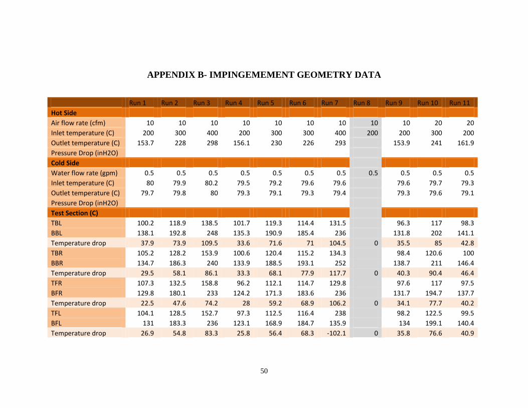
APPENDIX B- IMPINGEMEMENT GEOMETRY DATA
Run 1 Run 2 Run 3 Run 4 Run 5 Run 6 Run 7 Run 8 Run 9 Run 10 Run 11
Hot Side
Air flow rate (cfm) 10 10 10 10 10 10 10 10 10 20 20
Inlet temperature (C) 200 300 400 200 300 300 400 200 200 300 200
Outlet temperature (C) 153.7 228 298 156.1 230 226 293 153.9 241 161.9
Pressure Drop (inH2O)
Cold Side
Water flow rate (gpm) 0.5 0.5 0.5 0.5 0.5 0.5 0.5 0.5 0.5 0.5 0.5
Inlet temperature (C) 80 79.9 80.2 79.5 79.2 79.6 79.6 79.6 79.7 79.3
Outlet temperature (C) 79.7 79.8 80 79.3 79.1 79.3 79.4 79.3 79.6 79.1
Pressure Drop (inH2O)
Test Section (C)
TBL 100.2 118.9 138.5 101.7 119.3 114.4 131.5 96.3 117 98.3
BBL 138.1 192.8 248 135.3 190.9 185.4 236 131.8 202 141.1
Temperature drop 37.9 73.9 109.5 33.6 71.6 71 104.5 0 35.5 85 42.8
TBR 105.2 128.2 153.9 100.6 120.4 115.2 134.3 98.4 120.6 100
BBR 134.7 186.3 240 133.9 188.5 193.1 252 138.7 211 146.4
Temperature drop 29.5 58.1 86.1 33.3 68.1 77.9 117.7 0 40.3 90.4 46.4
TFR 107.3 132.5 158.8 96.2 112.1 114.7 129.8 97.6 117 97.5
BFR 129.8 180.1 233 124.2 171.3 183.6 236 131.7 194.7 137.7
Temperature drop 22.5 47.6 74.2 28 59.2 68.9 106.2 0 34.1 77.7 40.2
TFL 104.1 128.5 152.7 97.3 112.5 116.4 238 98.2 122.5 99.5
BFL 131 183.3 236 123.1 168.9 184.7 135.9 134 199.1 140.4
Temperature drop 26.9 54.8 83.3 25.8 56.4 68.3 -102.1 0 35.8 76.6 40.9

51
Run 12 Run 13 Run 14 Run 15 Run 16 Run 17 Run 18 Run 19 Run 20 Run 21 Run 22 Run 23 Run 24 Run 25
20 20 20 20 20 20 20 20 20 20 10 10 10 10
400 200 300 400 200 300 400 200 300 400 300 200 400 200
312 161.7 236 313 161.8 240 312 161.7 235 312 225
295 153.7
0.5 0.5 0.5 0.5 0.3 0.3 0.3 0.3 0.3 0.3 0.3 0.3 0.3 0.3
79.8 80.4 80.1 79.5 79.9 79.5 80.2 80 79.5 79.6 79.4 79.6 80.6 80.2
79.7 80.1 79.9 79.5 79.7 79.4 80.1 79.7 79.3 79.6 79.1 79.4 80.4 80.1
134.5 99.2 115 140 99.6 119.5 138.7 99.6 117.4 137.6 113.5 97.1 132.3 97.5
258 140.5 196.5 245 137.1 188.9 244 136.8 189.4 243 176.7 129.7 223 129.5
123.5 41.3 81.5 105 37.5 69.4 105.3 37.2 72 105.4 63.2 32.6 90.7 32
141 101 120.4 140.6 100.3 119.5 139.4 100.1 118.6 140.2 112.2 95.9 131.1 97.5
273 146.7 210 271 143.8 206 209 143 204 207 190.2 135.8 246 135.7
132 45.7 89.6 130.4 43.5 86.5 69.6 42.9 85.4 66.8 78 39.9 114.9 38.2
133.6 100.8 120.7 141.6 100.7 119.2 140.4 100.8 117.7 138.9 113.8 98 134.5 99.3
255 138.6 194.9 255 138.2 193.1 253 137.4 193.8 254 181.8 131.6 234 131.9
121.4 37.8 74.2 113.4 37.5 73.9 112.6 36.6 76.1 115.1 68 33.6 99.5 32.6
141.2 100.6 121.7 142 101.6 124.5 146.4 100.4 123.9 145.9 123.9 103.2 145.6 100.9
258 139.8 198.9 259 139.9 198.9 260 139.1 198.9 260 187.1 134.2 240 133.2
116.8 39.2 77.2 117 38.3 74.4 113.6 38.7 75 114.1 63.2 31 94.4 32.3

52
Run 26 Run 27 Run 28 Run 29 Run 30 Run 31 Run 32 Run 33 Run 34 Run 35 Run 36 Run 37 Run 38 Run 39
10 10 25 25 25 25 25 25 25 25 20 10 10 10
300 400 200 300 200 300 300 200 200 300 400 400 300 300
226 295 163.2 243 162.3 243 239 162.1
239 314 296 228 229
0.3 0.3 0.3 0.3 0.3 0.3 0.5 0.5 0.5 0.5 0.5 0.5 0.5 0.5
80.1 79.7 79.3 80.4 79.6 79.9 80.5 79.6 79.6 80.3 80.8 79.9 79.2 79.9
79.7 79.5 79.3 80.2 79.4 79.6 80.4 79.3 79.4 80 80.6 79.7 79.2 79.6
113.8 132.7 99.5 118.9 99.2 117.3 119.2 99.2 99.6 119.6 140.4 133.1 114.2 115.1
175.7 224 137.6 190.3 137.3 190.1 189.2 136.9 137.1 189.8 239 228 174.5 175.3
61.9 91.3 38.1 71.4 38.1 72.8 70 37.7 37.5 70.2 98.6 94.9 60.3 60.2
112.6 130.7 99.6 118 99.2 117.3 118 99.1 99.1 117.8 135.6 129.5 112.3 112.3
188.9 246 143.7 205 143.4 205 206 144.6 144.5 206 264 246 188.4 188.5
76.3 115.3 44.1 87 44.2 87.7 88 45.5 45.4 88.2 128.4 116.5 76.1 76.2
115.6 133.5 101 120.5 100.4 119.6 120.3 101.1 101 119 139 130.5 112.5 112.6
182.5 235 141.7 198.7 140.5 199 199.6 140.7 140.3 199.2 255 235 181.2 181.9
66.9 101.5 40.7 78.2 40.1 79.4 79.3 39.6 39.3 80.2 116 104.5 68.7 69.3
124.3 145.3 106.1 103.5 106.9 131.7 131.6 106.6 106.4 131.3 145.3 141.5 122.3 122.9
187.4 243 142.5 204 143.1 206 205 142.6 141.6 205 261 241 183.6 183.6
63.1 97.7 36.4 100.5 36.2 74.3 73.4 36 35.2 73.7 115.7 99.5 61.3 60.7
Related Documents