4-1 ME 306 Fluid Mechanics II Part 4 Compressible Flow These presentations are prepared by Dr. Cüneyt Sert Department of Mechanical Engineering Middle East Technical University Ankara, Turkey [email protected] Please ask for permission before using them. You are NOT allowed to modify them.

Welcome message from author
This document is posted to help you gain knowledge. Please leave a comment to let me know what you think about it! Share it to your friends and learn new things together.
Transcript
4-1
ME 306 Fluid Mechanics II
Part 4
Compressible Flow
These presentations are prepared by
Dr. Cüneyt Sert
Department of Mechanical Engineering
Middle East Technical University
Ankara, Turkey
Please ask for permission before using them. You are NOT allowed to modify them.
4-2
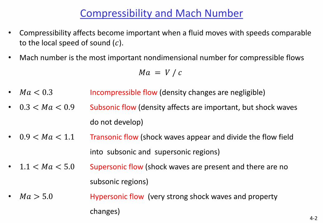
Compressibility and Mach Number
• Compressibility affects become important when a fluid moves with speeds comparable to the local speed of sound (𝑐).
• Mach number is the most important nondimensional number for compressible flows
𝑀𝑎 = 𝑉 / 𝑐
• 𝑀𝑎 < 0.3 Incompressible flow (density changes are negligible)
• 0.3 < 𝑀𝑎 < 0.9 Subsonic flow (density affects are important, but shock waves
do not develop)
• 0.9 < 𝑀𝑎 < 1.1 Transonic flow (shock waves appear and divide the flow field
into subsonic and supersonic regions)
• 1.1 < 𝑀𝑎 < 5.0 Supersonic flow (shock waves are present and there are no
subsonic regions)
• 𝑀𝑎 > 5.0 Hypersonic flow (very strong shock waves and property
changes)
4-3
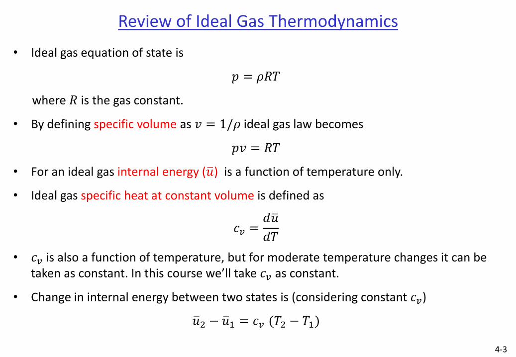
Review of Ideal Gas Thermodynamics
• Ideal gas equation of state is
𝑝 = 𝜌𝑅𝑇
where 𝑅 is the gas constant.
• By defining specific volume as 𝑣 = 1/𝜌 ideal gas law becomes
𝑝𝑣 = 𝑅𝑇
• For an ideal gas internal energy (𝑢 ) is a function of temperature only.
• Ideal gas specific heat at constant volume is defined as
𝑐𝑣 =𝑑𝑢
𝑑𝑇
• 𝑐𝑣 is also a function of temperature, but for moderate temperature changes it can be taken as constant. In this course we’ll take 𝑐𝑣 as constant.
• Change in internal energy between two states is (considering constant 𝑐𝑣)
𝑢 2 − 𝑢 1 = 𝑐𝑣 (𝑇2 − 𝑇1)

4-4
Review of Ideal Gas Thermodynamics (cont’d)
• Enthalpy is defined as
ℎ = 𝑢 +𝑝
𝜌 = 𝑢 + 𝑅𝑇
• For an ideal gas enthalpy is also a function of temperature only.
• Ideal gas specific heat at constant pressure is defined as
𝑐𝑝 =𝑑ℎ
𝑑𝑇
• 𝑐𝑝 will also be taken as constant in this course. For constant 𝑐𝑝 change in enthalpy is
ℎ2 − ℎ1 = 𝑐𝑝 (𝑇2 − 𝑇1)
• Combining the definition of 𝑐𝑣 and 𝑐𝑝
𝑐𝑝 − 𝑐𝑣 = 𝑑ℎ
𝑑𝑇−𝑑𝑢
𝑑𝑇 = 𝑅
4-5
Review of Ideal Gas Thermodynamics (cont’d)
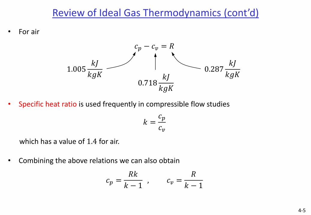
• For air
𝑐𝑝 − 𝑐𝑣 = 𝑅
• Specific heat ratio is used frequently in compressible flow studies
𝑘 =𝑐𝑝
𝑐𝑣
which has a value of 1.4 for air.
• Combining the above relations we can also obtain
𝑐𝑝 =𝑅𝑘
𝑘 − 1 , 𝑐𝑣 =
𝑅
𝑘 − 1
1.005𝑘𝐽
𝑘𝑔𝐾
0.718𝑘𝐽
𝑘𝑔𝐾
0.287𝑘𝐽
𝑘𝑔𝐾

4-6
Review of Ideal Gas Thermodynamics (cont’d)
• Entropy change for an ideal gas are expressed with 𝑇𝑑𝑠 relations
𝑇𝑑𝑠 = 𝑑𝑢 + 𝑝 𝑑1
𝜌 , 𝑇𝑑𝑠 = 𝑑ℎ −
1
𝜌 𝑑𝑝
• Integrating these 𝑇𝑑𝑠 relations for an ideal gas
𝑠2 − 𝑠1 = 𝑐𝑣 𝑙𝑛𝑇2𝑇1
+ 𝑅 𝑙𝑛𝜌1𝜌2
, 𝑠2 − 𝑠1 = 𝑐𝑝 𝑙𝑛𝑇2𝑇1
− 𝑅 𝑙𝑛𝑝2𝑝1
• For an adiabatic (no heat transfer) and frictionless flow, which is known as isentropic flow, entropy remains constant.
Exercise : For isentropic flow of an ideal gas with constant specific heat values, derive the following commonly used relations, known as isentropic relations
𝑇2𝑇1
𝑘/(𝑘−1)
=𝜌2𝜌1
𝑘
=𝑝2𝑝1

4-7
Speed of Sound (𝑐)
• Speed of sound is the rate of propagation of a pressure pulse (wave) of infinitesimal strength through a still medium (a fluid in our case).
• It is a thermodynamic property of the fluid.
• For air at standard conditions, sound moves with a speed of 𝑐 = 343 𝑚/𝑠
http://paws.kettering.edu/~drussell/demos.html
4-8
Speed of Sound (cont’d)
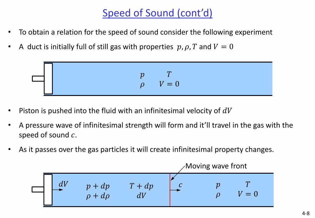
• To obtain a relation for the speed of sound consider the following experiment
• A duct is initially full of still gas with properties 𝑝, 𝜌, 𝑇 and 𝑉 = 0
• Piston is pushed into the fluid with an infinitesimal velocity of 𝑑𝑉
• A pressure wave of infinitesimal strength will form and it’ll travel in the gas with the speed of sound 𝑐.
• As it passes over the gas particles it will create infinitesimal property changes.
𝑝 𝜌
𝑇 𝑉 = 0
𝑑𝑉 𝑝 + 𝑑𝑝 𝜌 + 𝑑𝜌
𝑐 𝑝 𝜌
𝑇 + 𝑑𝑝 𝑑𝑉
𝑇 𝑉 = 0
Moving wave front

4-9
Speed of Sound (cont’d)
• For an observer moving with the wave front with speed 𝑐, wave front will be stationary and the fluid on the left and the right would move with relative speeds
• Consider a control volume enclosing the stationary wave front. The flow is one dimensional and steady.
𝑝 𝜌
𝑇 𝑉 = 𝑐
Stationary wave front
𝑝 + 𝑑𝑝 𝜌 + 𝑑𝜌
𝑇 + 𝑑𝑝 𝑉 = 𝑐 − 𝑑𝑉
in out
Cross sectional area 𝐴
4-10
Speed of Sound (cont’d)
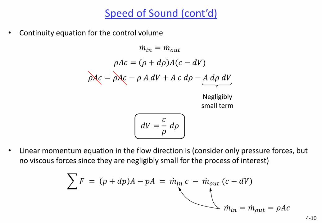
• Continuity equation for the control volume
𝑚 𝑖𝑛 = 𝑚 𝑜𝑢𝑡
𝜌𝐴𝑐 = 𝜌 + 𝑑𝜌 𝐴(𝑐 − 𝑑𝑉)
𝜌𝐴𝑐 = 𝜌𝐴𝑐 − 𝜌 𝐴 𝑑𝑉 + 𝐴 𝑐 𝑑𝜌 − 𝐴 𝑑𝜌 𝑑𝑉
𝑑𝑉 =𝑐
𝜌 𝑑𝜌
• Linear momentum equation in the flow direction is (consider only pressure forces, but no viscous forces since they are negligibly small for the process of interest)
𝐹 = 𝑝 + 𝑑𝑝 𝐴 − 𝑝𝐴 = 𝑚 𝑖𝑛 𝑐 − 𝑚 𝑜𝑢𝑡 (𝑐 − 𝑑𝑉)
Negligibly small term
𝑚 𝑖𝑛 = 𝑚 𝑜𝑢𝑡 = 𝜌𝐴𝑐
4-11
Speed of Sound (cont’d)
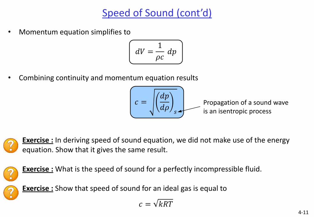
• Momentum equation simplifies to
𝑑𝑉 =1
𝜌𝑐 𝑑𝑝
• Combining continuity and momentum equation results
𝑐 =𝑑𝑝
𝑑𝜌𝑠
Exercise : In deriving speed of sound equation, we did not make use of the energy equation. Show that it gives the same result.
Exercise : What is the speed of sound for a perfectly incompressible fluid.
Exercise : Show that speed of sound for an ideal gas is equal to
𝑐 = 𝑘𝑅𝑇
Propagation of a sound wave is an isentropic process
4-12
Wave Propagation in a Compressible Fluid
• Consider a point source generating small pressure pulses (sound waves) at regular intervals.
• Case 1 : Stationary source
• Waves travel in all directions symmetrically.
• The same sound frequency will be heard everywhere around the source.
4-13
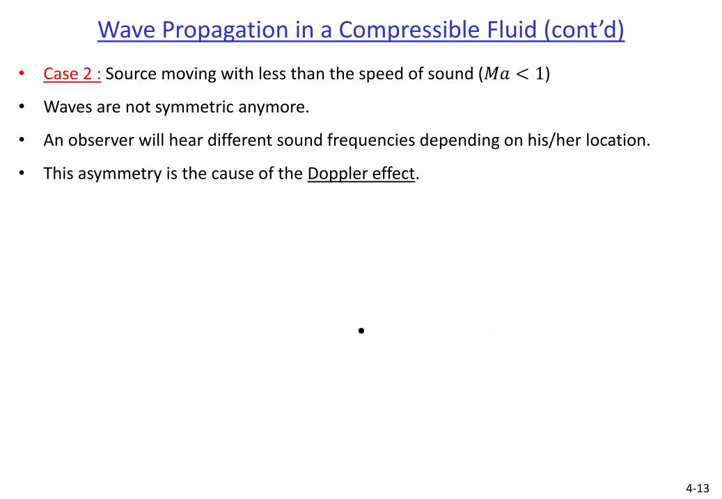
Wave Propagation in a Compressible Fluid (cont’d)
• Case 2 : Source moving with less than the speed of sound (𝑀𝑎 < 1)
• Waves are not symmetric anymore.
• An observer will hear different sound frequencies depending on his/her location.
• This asymmetry is the cause of the Doppler effect.
4-14
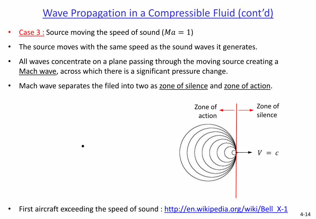
Wave Propagation in a Compressible Fluid (cont’d)
• Case 3 : Source moving the speed of sound (𝑀𝑎 = 1)
• The source moves with the same speed as the sound waves it generates.
• All waves concentrate on a plane passing through the moving source creating a Mach wave, across which there is a significant pressure change.
• Mach wave separates the filed into two as zone of silence and zone of action.
Zone of
action
Zone of silence
𝑉 = 𝑐
• First aircraft exceeding the speed of sound : http://en.wikipedia.org/wiki/Bell_X-1
4-15
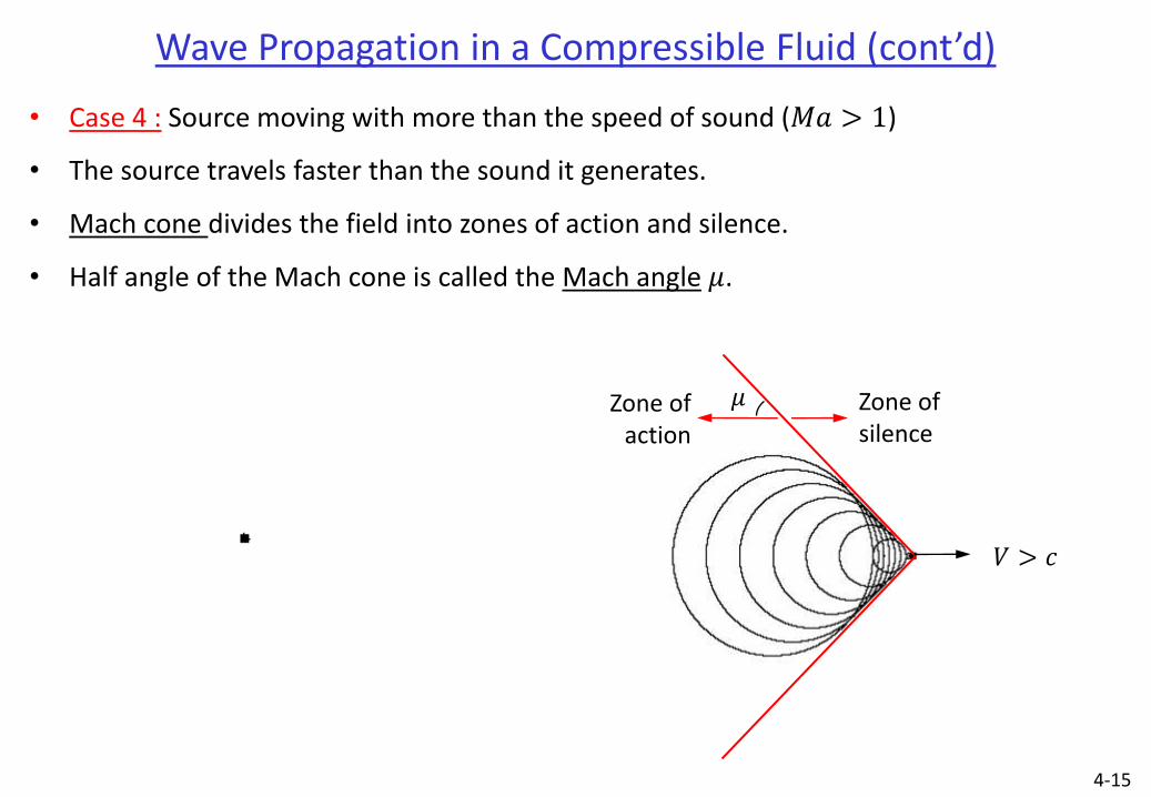
Wave Propagation in a Compressible Fluid (cont’d)
• Case 4 : Source moving with more than the speed of sound (𝑀𝑎 > 1)
• The source travels faster than the sound it generates.
• Mach cone divides the field into zones of action and silence.
• Half angle of the Mach cone is called the Mach angle 𝜇.
Zone of action
Zone of silence
𝑉 > 𝑐
𝜇
4-16
Wave Propagation in a Compressible Fluid (cont’d)
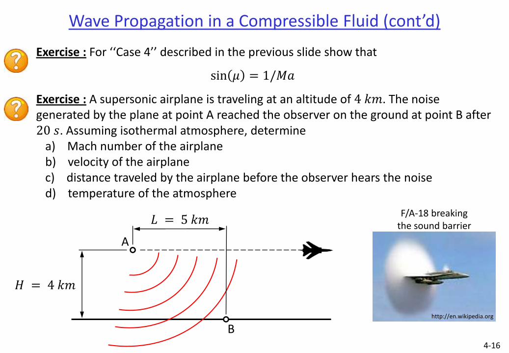
Exercise : For ‘‘Case 4’’ described in the previous slide show that
sin 𝜇 = 1/𝑀𝑎
Exercise : A supersonic airplane is traveling at an altitude of 4 𝑘𝑚. The noise generated by the plane at point A reached the observer on the ground at point B after 20 𝑠. Assuming isothermal atmosphere, determine
a) Mach number of the airplane b) velocity of the airplane c) distance traveled by the airplane before the observer hears the noise d) temperature of the atmosphere
A
B
𝐻 = 4 𝑘𝑚
𝐿 = 5 𝑘𝑚 F/A-18 breaking
the sound barrier
http://en.wikipedia.org

4-17
One Dimensional, Isentropic, Compressible Flow
• Consider an internal compressible flow, such as the one in a duct of variable cross sectional area
• Flow and fluid properties inside this nozzle change due to
• Cross sectional area change
• Frictional effects
• Heat transfer effects
• In ME 306 we’ll only study these flows to be one dimensional and consider only the effect of area change, i.e. assume isentropic flow.
NOT the subject of ME 306

• Energy balance between sections 1 and 2 is
ℎ1 +𝑉12
2+ 𝑔𝑧1 = ℎ2 +
𝑉22
2+ 𝑔𝑧2 − 𝑞 + 𝑤𝑓
• For gas flows potential energy change is negligibly small compared to kinetic energy change. Energy equation reduces to
ℎ1 +𝑉12
2= ℎ2 +
𝑉22
2
4-18
1D, Isentropic Flow (cont’d)
1 2
Heat transfer and friction work is neglected for
isentropic flow

• The sum ℎ +𝑉2
2 is known as stagnation enthalpy and it is constant inside the duct.
ℎ0 = ℎ +𝑉2
2 = constant
• It is called ‘‘stagnation’’ enthalpy because a stagnation point has zero velocity and the enthalpy of the gas is equal to ℎ0 at such a point.
4-19
Stagnation Enthalpy
stagnation enthalpy
Fluid in this large reservoir is almost stagnant. This reservoir is said to be at stagnation state.
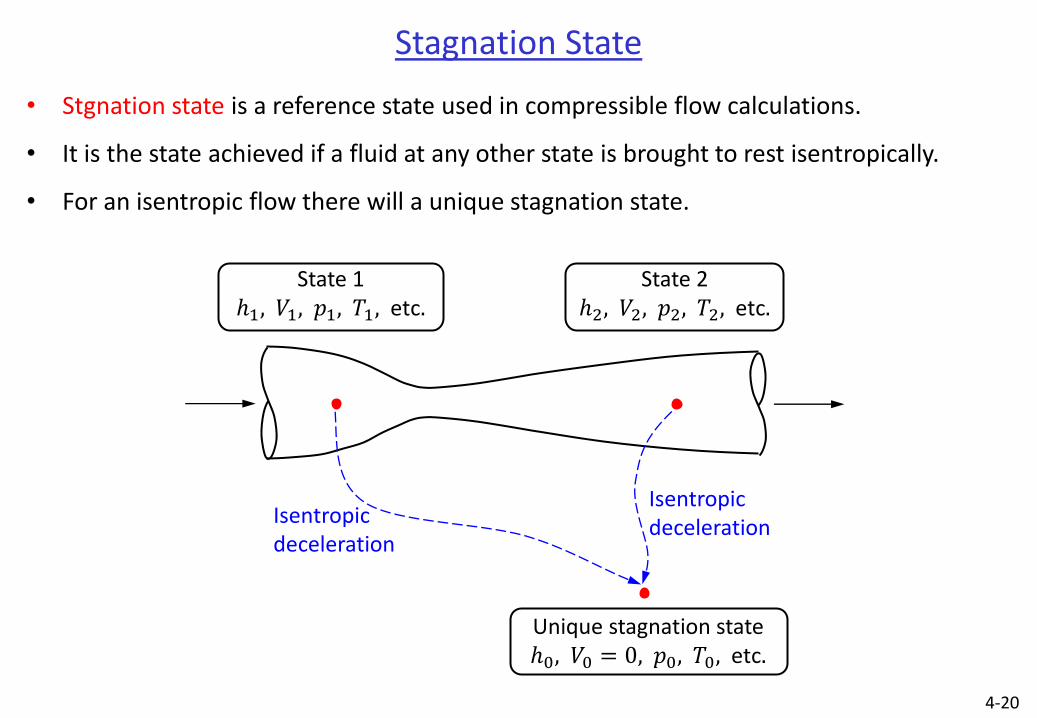
• Stgnation state is a reference state used in compressible flow calculations.
• It is the state achieved if a fluid at any other state is brought to rest isentropically.
• For an isentropic flow there will a unique stagnation state.
4-20
Stagnation State
State 1 ℎ1, 𝑉1, 𝑝1, 𝑇1, etc.
Isentropic deceleration
Isentropic deceleration
State 2 ℎ2, 𝑉2, 𝑝2, 𝑇2, etc.
Unique stagnation state ℎ0, 𝑉0 = 0, 𝑝0, 𝑇0, etc.

• Isentropic deceleration can be shown on a ℎ − 𝑠 diagram as follows
4-21
Stagnation State (cont’d)
• During isentropic deceleraion entropy remains constant.
• Energy conservation: ℎ0 +02
2= ℎ +
𝑉2
2 → ∆ℎ = ℎ0 − ℎ =
𝑉2
2
Isentropic deceleration
ℎ0
ℎ
ℎ
𝑠
𝑝0
𝑝
𝑉2/2
Any state ℎ, 𝑉, 𝑝, 𝑇, 𝑠, etc.
Stagnation state ℎ0, 𝑉0 = 0, 𝑝0, 𝑇0, 𝑠0, etc.

• For an ideal gas this enthalpy change can be expressed as a temperature change
𝑐𝑝∆𝑇 = ∆ℎ
𝑐𝑝(𝑇0 − 𝑇) =𝑉2
2
𝑇0 = 𝑇 +𝑉2
2𝑐𝑝
• During the isentropic deceleration temperature of the gas increases by 𝑉2
2𝑐𝑝.
Exercise : An airplane is crusing at a speed of 900 𝑘𝑚/ℎ at an altitude of 10 𝑘𝑚. Atmospheric air at −60 ℃ comes to rest at the tip of its pitot tube. Determine the temperature rise of air.
Read about heating of space shuttle during its reentry to the earth’s atmosphere.
http://en.wikipedia.org/wiki/Space_Shuttle_thermal_protection_system 4-22
Stagnation State (cont’d)

Exercise : For the flow of air as an ideal gas, express the following ratios as a function of Mach number and generate the following plot.
𝑇
𝑇0
𝑝
𝑝0
𝜌
𝜌0
𝑐
𝑐0
4-23
Stagnation State (cont’d)
1.0
0.5
0 1 2 3 4 5
Adapted from White’s Fluid Mechanics book
𝑀𝑎
𝑐
𝑐0 𝑇
𝑇0
𝜌
𝜌0 𝑝
𝑝0
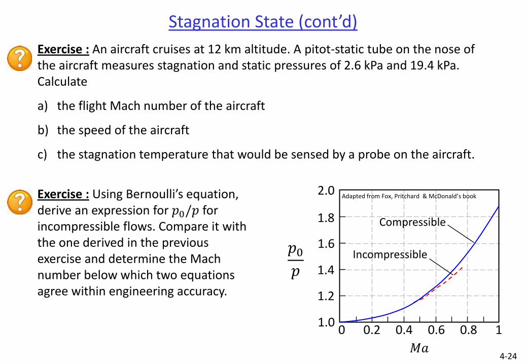
Exercise : Using Bernoulli’s equation, derive an expression for 𝑝0/𝑝 for incompressible flows. Compare it with the one derived in the previous exercise and determine the Mach number below which two equations agree within engineering accuracy.
4-24
Stagnation State (cont’d)
2.0
1.4
0 0.2 0.4 0.6 0.8 1
Adapted from Fox, Pritchard & McDonald’s book
𝑀𝑎
1.8
1.6
1.2
1.0
Compressible
Incompressible 𝑝0𝑝
Exercise : An aircraft cruises at 12 km altitude. A pitot-static tube on the nose of the aircraft measures stagnation and static pressures of 2.6 kPa and 19.4 kPa. Calculate
a) the flight Mach number of the aircraft
b) the speed of the aircraft
c) the stagnation temperature that would be sensed by a probe on the aircraft.

Exercise : Consider the differential control volume shown below for 1D, isentropic flow of an ideal gas through a variable area duct. Using conservation of mass, linear momentum and energy, determine the
a) Change of pressure with area
b) Change of velocity with area
4-25
Simple Area Change Flows (1D Isentropic Flows)
𝑝 𝜌 𝑉 ℎ 𝐴
𝑝 + 𝑑𝑝 𝜌 + 𝑑𝜌 𝑉 + 𝑑𝑉 ℎ + 𝑑ℎ 𝐴 + 𝑑𝐴
𝑑𝑥
𝑥
4-26
Simple Area Change Flows (cont’d)
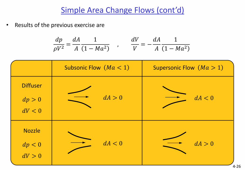
• Results of the previous exercise are
𝑑𝑝
𝜌𝑉2=𝑑𝐴
𝐴
1
1 − 𝑀𝑎2 ,
𝑑𝑉
𝑉= −
𝑑𝐴
𝐴
1
1 −𝑀𝑎2
𝑑𝐴 > 0
Diffuser
𝑑𝑝 > 0
𝑑𝑉 < 0
Nozzle
𝑑𝑝 < 0
𝑑𝑉 > 0
Subsonic Flow 𝑀𝑎 < 1 Supersonic Flow 𝑀𝑎 > 1
𝑑𝐴 < 0
𝑑𝐴 < 0
𝑑𝐴 > 0

4-27
Simple Area Change Flows (cont’d)
• Sonic flow is a very special case. It can occur
• when the cross sectional area goes through a minimum, i.e. 𝑑𝐴 = 0
• or at the exit of a subsonic nozzle or a supersonic diffuser
𝑀𝑎 < 1
𝑀𝑎 > 1
Sonic flow may occur at the throat.
Sonic flow may occur at these exits.

4-28
Simple Area Change Flows (cont’d)
Exercise : The nozzle shown on the right is called a converging diverging nozzle (de Laval nozzle). Show that it is the only way to
• isentropically accelerate a fluid from subsonic to supersonic speed.
• isentropically decelerate a fluid from supersonic to subsonic speed.
Exercise : When subsonic flow is accelerated in a nozzle, supersonic flow can never be achieved. At most Mach number can be unity at the exit.
What happens if we add another converging part to the exit of such a nozzle?
de Laval nozzle
𝑀𝑎 < 1 𝑀𝑎𝑒𝑥𝑖𝑡 = 1
𝑀𝑎 < 1
𝑀𝑎𝑒𝑥𝑖𝑡 =?

4-29
Critical State
• Critical state is the special state where Mach number is unity.
• It is a useful reference state, similar to stagnation state. It is useful even if there is no actual critical state in a flow.
• It is shown with an asterisk, like 𝑇∗, 𝑝∗, etc.
• Ratios derived in Slide 4-23 can be written using the critical state
𝑝𝑜𝑝∗
= 1 +𝑘 − 1
2
𝑘/(𝑘−1)
𝑇𝑜𝑇∗
= 1 +𝑘 − 1
2
𝜌𝑜𝜌∗
= 1 +𝑘 − 1
2
1/(𝑘−1)
𝑝𝑜𝑝= 1 +
𝑘 − 1
2𝑀𝑎2
𝑘/(𝑘−1)
𝑇𝑜𝑇= 1 +
𝑘 − 1
2𝑀𝑎2
𝜌𝑜𝜌= 1 +
𝑘 − 1
2𝑀𝑎2
1/(𝑘−1)
𝑀𝑎 = 1

4-30
Critical State (cont’d)
Exercise : Similar to the ratios given in the previous slide, following area ratio is also a function of Mach number and specific heat ratio only. Derive it.
𝐴
𝐴∗=
1
𝑀𝑎
1 +𝑘 − 12
𝑀𝑎2
𝑘 + 12
𝑘+12(𝑘−1)
3.0
0.5
0 0.5 1 1.5 2 2.5 3
Adapted from Fox, McDonald and Pritchard’s textbook 𝑘 = 1.4
𝑀𝑎
2.5
2.0
1.5
1.0
0
𝐴
𝐴∗
4-31
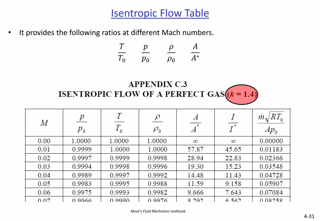
Isentropic Flow Table
• It provides the following ratios at different Mach numbers.
𝑇
𝑇0
𝑝
𝑝0
𝜌
𝜌0
𝐴
𝐴∗
Aksel’s Fluid Mechanics textbook
4-32
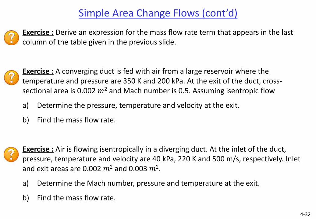
Simple Area Change Flows (cont’d)
Exercise : Derive an expression for the mass flow rate term that appears in the last column of the table given in the previous slide.
Exercise : A converging duct is fed with air from a large reservoir where the temperature and pressure are 350 K and 200 kPa. At the exit of the duct, cross-sectional area is 0.002 𝑚2 and Mach number is 0.5. Assuming isentropic flow
a) Determine the pressure, temperature and velocity at the exit.
b) Find the mass flow rate.
Exercise : Air is flowing isentropically in a diverging duct. At the inlet of the duct, pressure, temperature and velocity are 40 kPa, 220 K and 500 m/s, respectively. Inlet and exit areas are 0.002 𝑚2 and 0.003 𝑚2.
a) Determine the Mach number, pressure and temperature at the exit.
b) Find the mass flow rate.
4-33
Simple Area Change Flows (cont’d)
Exercise : Air flows isentropically in a channel. At an upstream section 1, Mach number is 0.3, area is 0.001 𝑚2, pressure is 650 kPa and temperature is 62 ℃. At a downstream section 2, Mach number is 0.8.
a) Sketch the channel shape.
b) Evaluate properties at section 2.
c) Plot the process between sections 1 and 2 on a 𝑇 − 𝑠 diagram.
4-34
Shock Waves
• Waves are disturbances (property changes) moving in a fluid.
• Sound wave is a weak wave, i.e. property changes across it are infinitesimally small.
• ∆𝑝 across a sound wave is in the order of 10−9 − 10−3 𝑎𝑡𝑚.
• Shock wave is a strong wave, i.e. property changes across it are finite.
• Shock waves are very thin, in the order of 10−7 𝑚.
• Fluid particles decelerate with tens of millions of 𝑔’s through a shock wave.
• They can be stationary or moving.
• They can be normal (perpendicular to the flow direction) or oblique (inclined to the flow direction).
• In ME 306 we’ll consider normal shock waves for 1D flows inside channels.
4-35
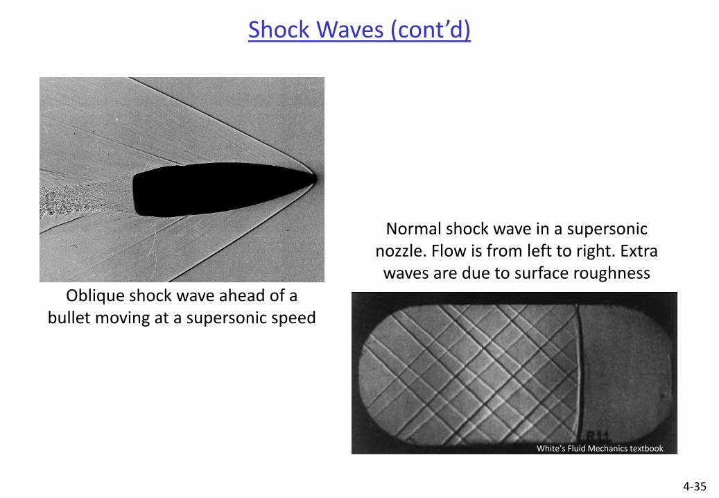
Oblique shock wave ahead of a bullet moving at a supersonic speed
Normal shock wave in a supersonic nozzle. Flow is from left to right. Extra waves are due to surface roughness
White’s Fluid Mechanics textbook
Shock Waves (cont’d)
4-36
Formation of a Strong Wave
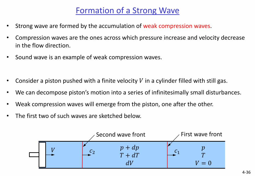
• Strong wave are formed by the accumulation of weak compression waves.
• Compression waves are the ones across which pressure increase and velocity decrease in the flow direction.
• Sound wave is an example of weak compression waves.
• Consider a piston pushed with a finite velocity 𝑉 in a cylinder filled with still gas.
• We can decompose piston’s motion into a series of infinitesimally small disturbances.
• Weak compression waves will emerge from the piston, one after the other.
• The first two of such waves are sketched below.
𝑉 𝑐1 𝑝 𝑇
𝑉 = 0
First wave front
𝑐2
Second wave front
𝑝 + 𝑑𝑝 𝑇 + 𝑑𝑇 𝑑𝑉
4-37
Formation of a Strong Wave (cont’d)
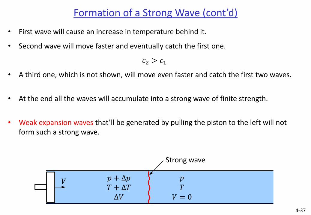
• First wave will cause an increase in temperature behind it.
• Second wave will move faster and eventually catch the first one.
𝑐2 > 𝑐1
• A third one, which is not shown, will move even faster and catch the first two waves.
• At the end all the waves will accumulate into a strong wave of finite strength.
• Weak expansion waves that’ll be generated by pulling the piston to the left will not form such a strong wave.
𝑉 𝑝 𝑇
𝑉 = 0
Strong wave
𝑝 + ∆𝑝 𝑇 + ∆𝑇 ∆𝑉
4-38
Property Changes Across a Shock Wave
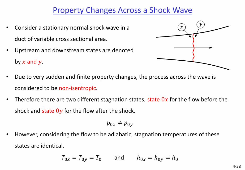
• Consider a stationary normal shock wave in a
duct of variable cross sectional area.
• Upstream and downstream states are denoted
by 𝑥 and 𝑦.
𝑥 𝑦
• Due to very sudden and finite property changes, the process across the wave is
considered to be non-isentropic.
• Therefore there are two different stagnation states, state 0𝑥 for the flow before the
shock and state 0𝑦 for the flow after the shock.
𝑝0𝑥 ≠ 𝑝0𝑦
• However, considering the flow to be adiabatic, stagnation temperatures of these
states are identical.
𝑇0𝑥 = 𝑇0𝑦 = 𝑇0 and ℎ0𝑥 = ℎ0𝑦 = ℎ0

• Stagnation state concept can also be used for non-isentropic flows, but there will be multiple such states.
• ℎ0 , 𝑇0 and 𝑐0 will be unique but not other stagnation properties such as 𝑝0 or 𝜌0.
4-39
Stagnation State of a Non-isentropic Flow
State 1 ℎ1, 𝑉1, 𝑝1, 𝑇1, etc.
Isentropic deceleration
Isentropic deceleration
State 2 ℎ2, 𝑉2, 𝑝2, 𝑇2, etc.
Stagnation state 2 ℎ0, 𝑉0 = 0, 𝑝02, 𝜌02, 𝑇0, etc.
Stagnation state 1 ℎ0, 𝑉0 = 0, 𝑝01, 𝜌01, 𝑇0, etc.
Non-isentropic flow
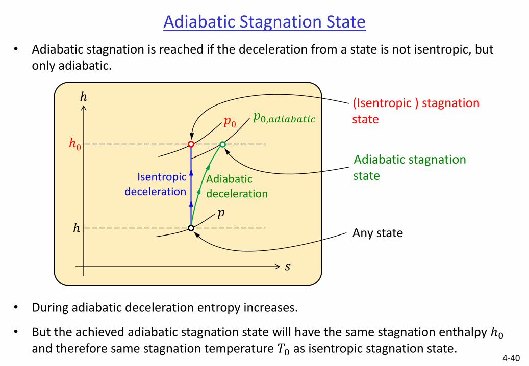
• Adiabatic stagnation is reached if the deceleration from a state is not isentropic, but only adiabatic.
4-40
Adiabatic Stagnation State
• During adiabatic deceleration entropy increases.
• But the achieved adiabatic stagnation state will have the same stagnation enthalpy ℎ0 and therefore same stagnation temperature 𝑇0 as isentropic stagnation state.
Isentropic deceleration
ℎ0
ℎ
ℎ
𝑠
𝑝0
𝑝
Any state
(Isentropic ) stagnation state 𝑝0,𝑎𝑑𝑖𝑎𝑏𝑎𝑡𝑖𝑐
Adiabatic stagnation state Adiabatic
deceleration
4-41
Property Changes Across a Shock Wave (cont’d)
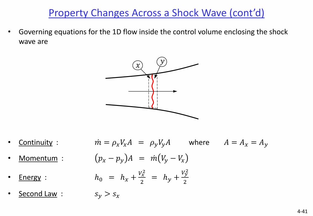
• Governing equations for the 1D flow inside the control volume enclosing the shock wave are
• Continuity : 𝑚 = 𝜌𝑥𝑉𝑥𝐴 = 𝜌𝑦𝑉𝑦𝐴 where 𝐴 = 𝐴𝑥 = 𝐴𝑦
• Momentum : 𝑝𝑥 − 𝑝𝑦 𝐴 = 𝑚 𝑉𝑦 − 𝑉𝑥
• Energy : ℎ0 = ℎ𝑥 +𝑉𝑥2
2 = ℎ𝑦 +
𝑉𝑦2
2
• Second Law : 𝑠𝑦 > 𝑠𝑥
𝑥 𝑦
4-42
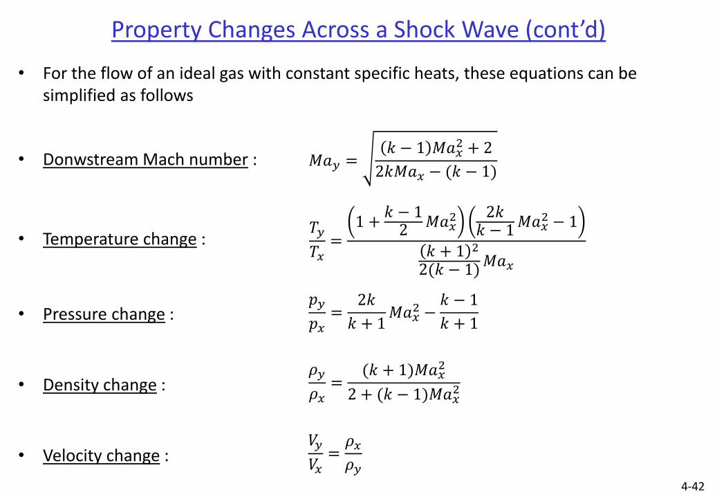
Property Changes Across a Shock Wave (cont’d)
• For the flow of an ideal gas with constant specific heats, these equations can be simplified as follows
• Donwstream Mach number :
• Temperature change :
• Pressure change :
• Density change :
• Velocity change :
𝑀𝑎𝑦 =𝑘 − 1 𝑀𝑎𝑥
2 + 2
2𝑘𝑀𝑎𝑥 − (𝑘 − 1)
𝑇𝑦
𝑇𝑥=
1 +𝑘 − 12 𝑀𝑎𝑥
2 2𝑘𝑘 − 1
𝑀𝑎𝑥2 − 1
𝑘 + 1 2
2(𝑘 − 1)𝑀𝑎𝑥
𝑝𝑦
𝑝𝑥=
2𝑘
𝑘 + 1𝑀𝑎𝑥
2 −𝑘 − 1
𝑘 + 1
𝜌𝑦
𝜌𝑥=
(𝑘 + 1)𝑀𝑎𝑥2
2 + (𝑘 − 1)𝑀𝑎𝑥2
𝑉𝑦
𝑉𝑥=𝜌𝑥𝜌𝑦
4-43
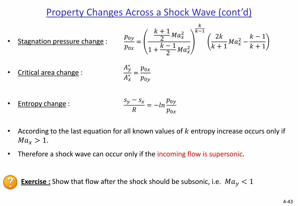
Property Changes Across a Shock Wave (cont’d)
• Stagnation pressure change :
• Critical area change :
• Entropy change :
• According to the last equation for all known values of 𝑘 entropy increase occurs only if 𝑀𝑎𝑥 > 1.
• Therefore a shock wave can occur only if the incoming flow is supersonic.
Exercise : Show that flow after the shock should be subsonic, i.e. 𝑀𝑎𝑦 < 1
𝑝0𝑦
𝑝0𝑥=
𝑘 + 12
𝑀𝑎𝑥2
1 +𝑘 − 12 𝑀𝑎𝑥
2
𝑘𝑘−1
2𝑘
𝑘 + 1𝑀𝑎𝑥
2 −𝑘 − 1
𝑘 + 1
𝐴𝑦∗
𝐴𝑥∗ =
𝑝0𝑥𝑝0𝑦
𝑠𝑦 − 𝑠𝑥
𝑅= −𝑙𝑛
𝑝0𝑦
𝑝0𝑥

4-44
Property Changes Across a Shock Wave (cont’d)
• All these relations are given as functions of 𝑀𝑎𝑥 and 𝑘 only.
• Usually graphical or tabulated forms of them are used.
Aksel’s Fluid Mechanics textbook
4-45
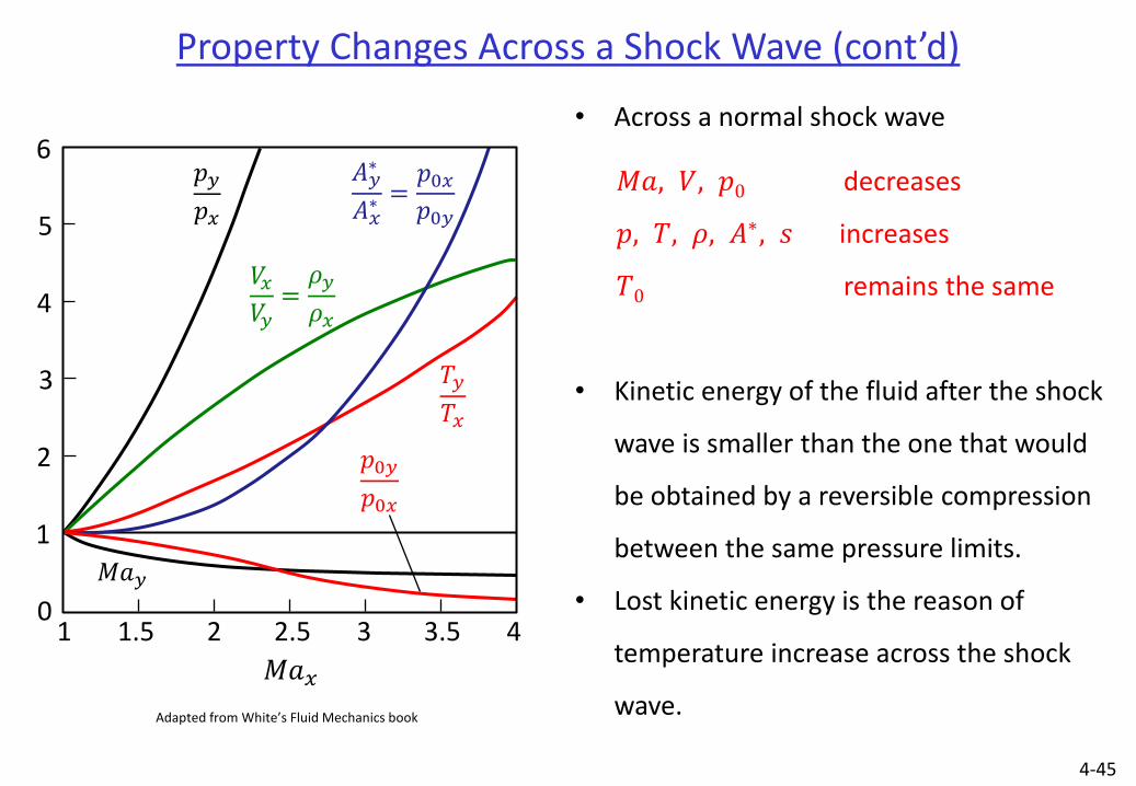
Property Changes Across a Shock Wave (cont’d)
6
1 1.5 2 2.5 3 3.5 4
Adapted from White’s Fluid Mechanics book
𝑀𝑎𝑥
5
4
3
2
1
0
𝑝𝑦
𝑝𝑥
𝑇𝑦
𝑇𝑥
𝐴𝑦∗
𝐴𝑥∗ =
𝑝0𝑥𝑝0𝑦
𝑉𝑥𝑉𝑦
=𝜌𝑦
𝜌𝑥
𝑝0𝑦
𝑝0𝑥
𝑀𝑎𝑦
• Across a normal shock wave
𝑀𝑎, 𝑉, 𝑝0 decreases
𝑝, 𝑇, 𝜌, 𝐴∗, 𝑠 increases
𝑇0 remains the same
• Kinetic energy of the fluid after the shock
wave is smaller than the one that would
be obtained by a reversible compression
between the same pressure limits.
• Lost kinetic energy is the reason of
temperature increase across the shock
wave.

4-46
Normal Shock Wave (cont’d)
Exercise : Air traveling at a Mach number of 1.8 undergoes a normal shock wave.
Stagnation properties before the shock are known as 𝑝0𝑥 = 150 𝑘𝑃𝑎, 𝑇0𝑥 = 350 𝐾.
Determine 𝑝𝑦 , 𝑇𝑦 , 𝑀𝑎𝑦 , 𝑉𝑦 , 𝑇0𝑦 , 𝑝0𝑦 , 𝑠𝑦 – 𝑠𝑥
Exercise : Supersonic air flow inside a diverging duct is slowed down by a normal
shock wave. Mach number at the inlet and exit of the duct are 2.0 and 0.3. Ratio of
the exit to inlet cross sectional areas is 2. Pressure at the inlet of the duct is 40 kPa.
Determine the pressure after the shock wave and at the exit of the duct.
4-47
Operation of a Converging Nozzle
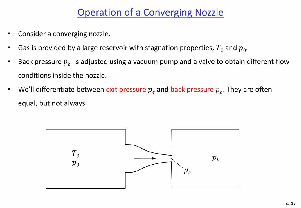
• Consider a converging nozzle.
• Gas is provided by a large reservoir with stagnation properties, 𝑇0 and 𝑝0.
• Back pressure 𝑝𝑏 is adjusted using a vacuum pump and a valve to obtain different flow
conditions inside the nozzle.
• We’ll differentiate between exit pressure 𝑝𝑒 and back pressure 𝑝𝑏. They are often
equal, but not always.
𝑇0
𝑝0 𝑝𝑒
𝑝𝑏
4-48
Operation of a Converging Nozzle (cont’d)
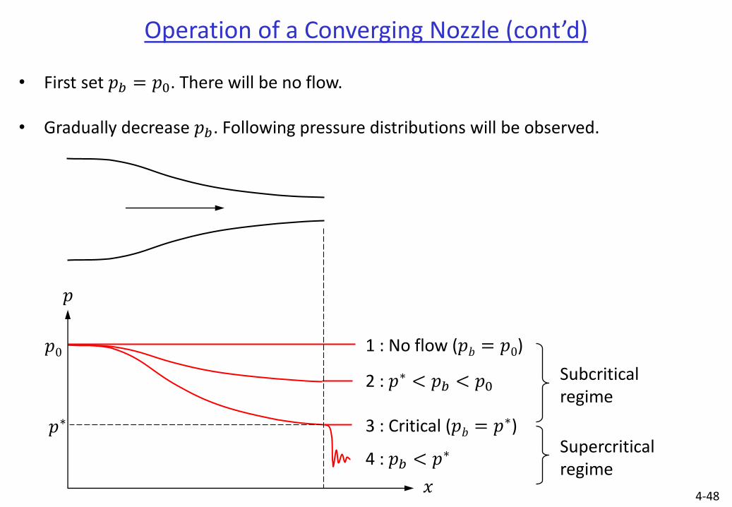
• First set 𝑝𝑏 = 𝑝0. There will be no flow.
• Gradually decrease 𝑝𝑏. Following pressure distributions will be observed.
𝑝
𝑥
1 : No flow (𝑝𝑏 = 𝑝0) 𝑝0
𝑝∗
2 : 𝑝∗ < 𝑝𝑏 < 𝑝0
3 : Critical (𝑝𝑏 = 𝑝∗)
Subcritical regime
4 : 𝑝𝑏 < 𝑝∗ Supercritical regime

4-49
Choked Flow
• Flow inside the converging nozzle always remain subsonic.
• For the subcritical regime as we decrease 𝑝𝑏 mass flow rate increases.
• State shown with * is the critical state. When 𝑝𝑏 is lowered to the critical value , exit
Mach number reaches to 1 and flow is said to be choked.
• If 𝑝𝑏 is lowered further, flow remains choked. Pressure and Mach number at the exit
does not change. Mass flow rate through the nozzle does not change.
• For 𝑝𝑏 < 𝑝∗, gas exits the nozzle as a supercritical jet with 𝑝𝑒 > 𝑝𝑏. It undergoes
through a number of alternating expansion waves and shocks and its cross sectional
area periodically becomes thinner and thicker.
4-50
Operation of a Converging Nozzle (cont’d)
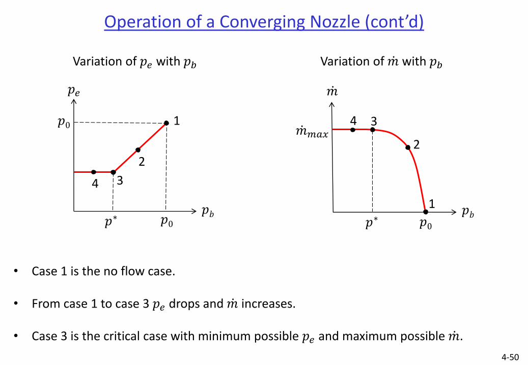
• Case 1 is the no flow case.
• From case 1 to case 3 𝑝𝑒 drops and 𝑚 increases.
• Case 3 is the critical case with minimum possible 𝑝𝑒 and maximum possible 𝑚 .
𝑝𝑏
2
1
3 4
𝑝∗ 𝑝0
𝑚
𝑚 𝑚𝑎𝑥
Variation of 𝑚 with 𝑝𝑏
2
1
3 4
𝑝0
𝑝𝑏 𝑝∗ 𝑝0
𝑝𝑒
Variation of 𝑝𝑒 with 𝑝𝑏
4-51
Operation of a Conv-Div Nozzle
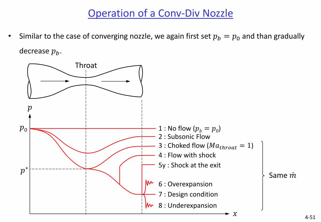
• Similar to the case of converging nozzle, we again first set 𝑝𝑏 = 𝑝0 and than gradually
decrease 𝑝𝑏.
Throat
𝑝
𝑥
1 : No flow (𝑝𝑏 = 𝑝0) 𝑝0
𝑝∗ 5y : Shock at the exit
Same 𝑚
2 : Subsonic Flow 3 : Choked flow (𝑀𝑎𝑡ℎ𝑟𝑜𝑎𝑡 = 1)
4 : Flow with shock
6 : Overexpansion
8 : Underexpansion
7 : Design condition
4-52
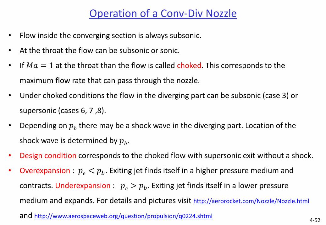
Operation of a Conv-Div Nozzle
• Flow inside the converging section is always subsonic.
• At the throat the flow can be subsonic or sonic.
• If 𝑀𝑎 = 1 at the throat than the flow is called choked. This corresponds to the
maximum flow rate that can pass through the nozzle.
• Under choked conditions the flow in the diverging part can be subsonic (case 3) or
supersonic (cases 6, 7 ,8).
• Depending on 𝑝𝑏 there may be a shock wave in the diverging part. Location of the
shock wave is determined by 𝑝𝑏.
• Design condition corresponds to the choked flow with supersonic exit without a shock.
• Overexpansion : 𝑝𝑒 < 𝑝𝑏. Exiting jet finds itself in a higher pressure medium and
contracts. Underexpansion : 𝑝𝑒 > 𝑝𝑏. Exiting jet finds itself in a lower pressure
medium and expands. For details and pictures visit http://aerorocket.com/Nozzle/Nozzle.html
and http://www.aerospaceweb.org/question/propulsion/q0224.shtml
4-53
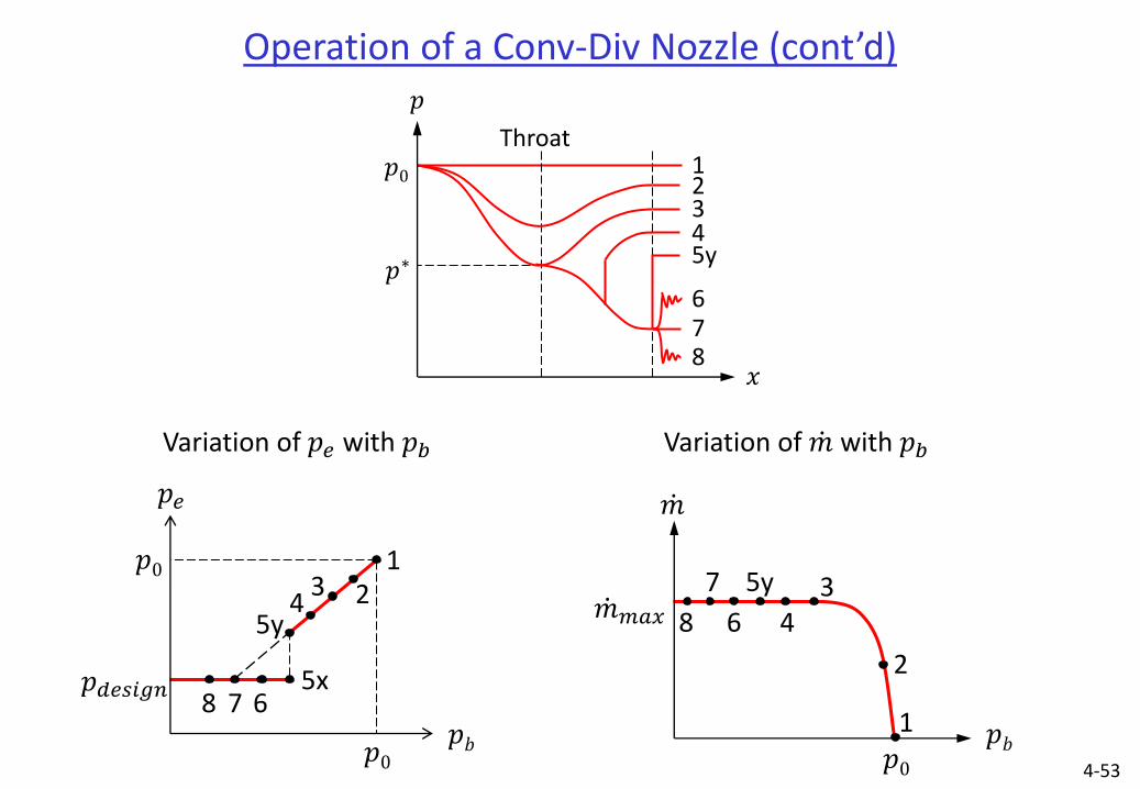
Operation of a Conv-Div Nozzle (cont’d)
5y
1 3
8
𝑝0
𝑝𝑏 𝑝0
𝑝𝑒
5x 7 6
4 2
Variation of 𝑝𝑒 with 𝑝𝑏
𝑝𝑑𝑒𝑠𝑖𝑔𝑛
𝑝
𝑥
1 𝑝0
𝑝∗ 5y
2 3 4
6
8 7
Throat
2
1
3 4
5y
6
7
8
𝑝𝑏 𝑝0
𝑚
𝑚 𝑚𝑎𝑥
Variation of 𝑚 with 𝑝𝑏
4-54
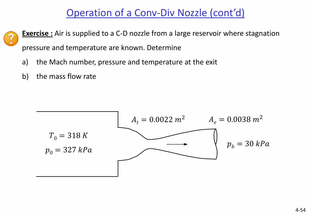
Operation of a Conv-Div Nozzle (cont’d)
Exercise : Air is supplied to a C-D nozzle from a large reservoir where stagnation
pressure and temperature are known. Determine
a) the Mach number, pressure and temperature at the exit
b) the mass flow rate
𝑇0 = 318 𝐾
𝑝0 = 327 𝑘𝑃𝑎
𝐴𝑒 = 0.0038 𝑚2
𝑝𝑏 = 30 𝑘𝑃𝑎
𝐴𝑡 = 0.0022 𝑚2
4-55
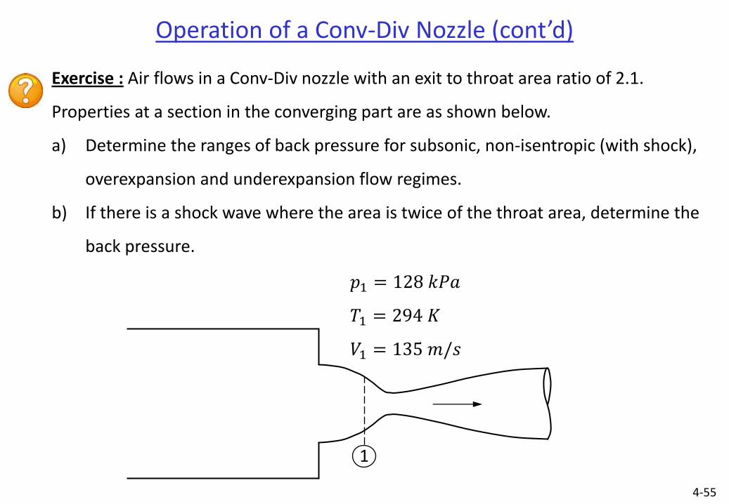
Operation of a Conv-Div Nozzle (cont’d)
Exercise : Air flows in a Conv-Div nozzle with an exit to throat area ratio of 2.1.
Properties at a section in the converging part are as shown below.
a) Determine the ranges of back pressure for subsonic, non-isentropic (with shock),
overexpansion and underexpansion flow regimes.
b) If there is a shock wave where the area is twice of the throat area, determine the
back pressure.
𝑝1 = 128 𝑘𝑃𝑎
𝑇1 = 294 𝐾
𝑉1 = 135 𝑚/𝑠
1
Related Documents


![Link Farmer[countryside] to Customer[downtown]. Downtown Valley F F F F F F F F.](https://static.cupdf.com/doc/110x72/56649f385503460f94c55132/link-farmercountryside-to-customerdowntown-downtown-valley-f-f-f-f-f-f.jpg)
